Estimation of Vector Error Correction Models with

Mixed-Frequency Data

Byeongchan Seonga, Sung K. Ahnb, and Peter A. Zadroznyc a Department of Statistics, Chung-Ang University, Seoul 156-756, Korea (e-mail: bcseong@cau.ac.kr) b Department of Management and Operations, Washington State University, Pullman, WA 99164-4736, USA (e-mail: ahn@wsu.edu) c Bureau of Labor Statistics,2 Massachusetts Ave., NE, Washington, DC 20212, USA (e-mail: Zadrozny.Peter@bls.gov)

Draft Date: October 2, 2008

ABSTRACT

We develop a method for directly modeling cointegrated multivariate time series that

are observed in mixed frequencies. We regard lower-frequency data as regularly (or

irregularly) missing and treat them with higher-frequency data by adopting a state-

space model. This utilizes the structure of multivariate data as well as the available

sample information more fully than the methods of transformation to a single

frequency, and enables us to estimate parameters including cointegrating vectors and

the missing observations of low-frequency data and to construct forecasts for future

values. For the maximum likelihood estimation of the parameters in the model, we

use an expectation maximization algorithm based on the state-space representation of

the error correction model. The statistical efficiency of the developed method is

investigated through a Monte Carlo study. We apply the method to a mixed-

frequency data set that consists of the quarterly real gross domestic product and the

monthly consumer price index.

JEL classification: C13, C22, C32.

Keywords: missing data, cointegration, Kalman filter, expectation maximization

algorithm, smoothing

1. INTRODUCTION

Multivariate time series that arise in economics and business are often observed in

mixed frequencies. For example, data available from the database of the Bureau of

Economic Analysis, the Bureau of Labor Statistics, and the Bureau of the Census are

often in mixed frequencies, mostly with quarterly, monthly or weekly sampling

intervals. Although cointegration, which represents a long-run equilibrium among the

components of nonstationary multivariate time series, has been one of the most

extensively investigated research topics, especially, in economics and business during

the past two decades since Engle and Granger (1987), studies of cointegration have

been limited to the case where all the components of a multivariate series are observed

at the same frequency.

Data observed in mixed frequencies are usually transformed to a single

frequency by temporally aggregating higher-frequency data to lower frequencies, or by

interpolating lower-frequency data to higher frequencies. However, temporal

aggregation destroys sample information (Zadrozny 1990). Granger and Siklos

(1995) examined the misinterpretation of the long-run component of a time series

constructed by temporal aggregation. Marcellino (1999) theoretically derived the

effects of temporal aggregation on cointegration such as the asymptotic invariance of

cointegrating (CI) rank and vectors. However, he illustrated some possibilities of the

loss of power of cointegration tests due to a decline in the number of available

2

observations. Haug (2002) showed in Monte Carlo experiments with various

cointegration tests and data generating processes (DGPs) that these power losses

indeed occur and assessed their extents in samples of typical size used in empirical

work.

For the case of interpolation of mixed-frequency data, Chow and Lin (1971)

used the conventional regression approach, and Ghysels and Valkanov (2006) used the

projection of low-frequency data on high-frequency data. Other researchers, for

example, Bernanke et al. (1997), Cuche and Hess (2000), and Liu and Hall (2001),

used the state-space framework suggested by Harvey and Pierse (1984) where

interpolation is based on univariate regression. When the goal is to estimate a

multivariate model for forecasting or other purposes, this kind of interpolation is at

best an intermediate nuisance and at worst a source of distortion in the data to be used

for estimation (Zadrozny 1990, p. 2).

Recently, Mariano and Murasawa (henceforth, MM) (2003, 2004) considered

multivariate models for constructing a new index of economic indicators using mixed-

frequency data, which overcome the drawbacks of a univariate approach and exploit

the cross-frequency sample information. However, they used differenced data instead

of levels data. This causes a loss of information on the long-run dynamics among the

variables.

In this paper we develop a method for directly modeling the cointegrated

multivariate time series with mixed-frequency data, which is based on the state-space

representation of the error correction model (ECM). We use the state-space

formulation for mixed-frequency data in our development by fully utilizing the

structure of multivariate data as well as the available sample information. For the

analysis, we exploit an expectation maximization (EM) algorithm. The method is

3

applied to estimate the parameters and the missing observations of the low-frequency

variables and to construct forecasts of their future values.

The structure of the paper is as follows. In Section 2, we describe preliminary

concepts for mixed-frequency data and set up the state-space representation for the

ECM of cointegration. In Section 3, we develop the procedures for estimating the

parameters of the cointegrated model using the EM algorithm and discuss initial

conditions for the procedures. In Section 4, we comment on smoothing, forecasting,

logarithmic transformation, and models with different types of deterministic terms. In

Section 5, we conduct Monte Carlo experiments for the investigation of the

performance of the developed method. In Section 6, we consider a numerical

example to illustrate the method and we conclude the paper in Section 7.

2. MODEL WITH MIXED-FREQUENCY DATA

In this section, we define mixed-frequency data and the ECM for multivariate

cointegrated time series.

2.1 Mixed-frequency data

We define high-frequency variables as those observed at the shortest sampling interval

and define low-frequency variables as those observed at longer sampling intervals,

either as temporal aggregates or as skip samples of their high-frequency values. A

variable is skip sampled when, for example, it is generated every month but is sampled

every third month, say, in the last month of every quarter. We assume that the

underlying data generating process of a multivariate time series of mixed-frequency

data, composed of both the high and the low-frequency variables, operates at the

highest frequency, as in Zadrozny (1990), Ghysels and Valkanov (2006), and MM

4

(2003, 2004) among others. All variables are assumed to be produced at the highest

frequency, but some variables are not observed at the highest frequency. For example,

we consider a bivariate time series of the consumer price index (CPI) observed

monthly and the gross domestic product (GDP) observed quarterly. CPI is the high-

frequency variable and GDP is the low-frequency variable. The highest frequency is

monthly and GDP is in principle ‘produced’ monthly but is observed only quarterly.

Variables like GDP observed as temporal aggregates are often called flows, while

variables observed at the high frequency are often called stocks.

2.2 Error correction model and state-space representation

Let be an n-dimensional vector autoregressive process of order p, ,

which operates at the highest frequency with CI rank , and consider the

corresponding error correction form

tu )(VAR p

h

, (1) t

p

jjtjtt uubau ε+ΔΨ+′=Δ ∑

−

=−−

1

11

where a and b are matrices with hn× nh <<0 and dnh −= , , for

, are matrices, and

jΨ

1,,1 −= pj L nn× tε is an independent random

vector. We assume that the elements of are ordered such that the last

elements are not cointegrated. This assumption permits the normalization

),0( ΩnN

tu hnd −=

][ 0 ′′= βhIb for identification, as in Ahn and Reinsel (1990), where hI denotes an

identity matrix and h h× 0β is a hd × matrix. The characteristic equation of

model (1) has exactly roots equal to one and all other roots are assumed to be

outside the unit circle, so that is cointegrated of order (1,1) (Engle and Granger

1987).

d

tu

We reorder the elements of to form tu ),( 21 ′′′= ttt zzz such that an vector 11×n

5

tz1 corresponds to high-frequency variables and an 12 ×n vector corresponds to

low-frequency variables, where

tz2

21 nnn += . For brevity, we assume that the low-

frequency variables are observed as temporal aggregates because the method can be

easily modified to accommodate the alternative case of skip-sampled data. The

reordering implies , where V is an tt Vuz = nn× permutation matrix. Substituting

with and pre-multiplying both sides of equation (1) by V, we can rewrite

model (1) as

tu tzV 1−

, (2) t

p

jjtjtt ezzz +ΔΓ+′=Δ ∑

−

=−−

1

11βα

where Va=α , Vb=β , VV jj ′Ψ=Γ , tt Ve ε= , ),0(~ ΣNet , and VV ′Ω=Σ . Also,

note that . For convenience of estimation, we write VV ′=−1021 ββ VIV h += , where

and are 1V 2V hn× and matrices, such that dn× [ ]21 VVV = . The VAR(p)

representation of model (2) is

, (3) t

p

jjtjt ezz +Φ=∑

=−

1

where 11 Γ+′+=Φ βαnI , 1−Γ−Γ=Φ jjj , for 1,,2 −= pj L , and 1−Γ−=Φ pp .

In practice, as mentioned above, the low-frequency variables, , are not

observed directly at the highest frequency, but either as temporally-aggregated flows or

as skip-sampled stocks. Flows can be expressed as

tz2

2 0

vt jj 2t jy C z −==∑ , where v

denotes the maximum degree of aggregation and the ’s are diagonal

indicator matrices with zeros and ones on the principal diagonal. By adjusting the

diagonal elements of , Zadrozny (1990) suggested a way to treat a variable which is

observed directly as a stock, but with a delay.

jC 22 nn ×

jC

We now construct a state-space representation of model (3). Let the state 1×s

6

vector , where 1( , , )t t t rx z z − +′ ′= L ′ max( , 1)r p v= + and s nr= for .

Then, we define the state equation, as in Zadrozny (1990), by

Tt ,,1 L=

ttt GeFxx += −1 , (4)

where the initial state, , is assumed to be a normal random vector with mean vector 0x

λ and covariance matrix ss× Λ . Here, and denote and

matrices defined by

F G ss× ns×

1 2 r

n n n

n n n

n n n

I O OF O I O

O O O

Φ Φ Φ⎡ ⎤⎢ ⎥⎢ ⎥⎢ ⎥=⎢ ⎥⎢ ⎥⎢ ⎥⎣ ⎦

L

L

L

M M L M

L

, , ⎥⎦

⎤⎢⎣

⎡=

×− nns

n

OI

G)(

nj O=Φ if pj > ,

where and denote and nO nmO × n n× nm× zero matrices, respectively.

Next, assuming no observation errors, we define the measurement equation

, (5) tt

tt x

HH

yy

y ⎟⎟⎠

⎞⎜⎜⎝

⎛=⎟⎟

⎠

⎞⎜⎜⎝

⎛≡

2

1

2

1

where

tt zy 11 = , [ ])(1 nsnn OIH −× 111≡ ,

[ ]2 1 2 1 2 12 0 1n n n n n n rH O C O C O C× × ×≡ L 1− n, and 2jC O= if vj > .

The matrix picks out the high-frequency variables from state vector and the

matrix picks out the low-frequency variables from the state vector as temporal

aggregates. We introduce a new series, , which is observed only at lower

frequencies, in order to deal with the missing observations in . As in Brockwell

and Davis (1991), we fill in missing observations of with random vectors which

are independent of and are distributed independently of the parameters in model

(2). Accordingly, we modify measurement equation (5) as

1H tx

2H

+ty2

ty2

ty2

ty

7

, (6) tt

nnt

tt

tt w

QO

xHH

yy

y ⎟⎟⎠

⎞⎜⎜⎝

⎛+⎟⎟

⎠

⎞⎜⎜⎝

⎛=⎟⎟

⎠

⎞⎜⎜⎝

⎛≡ ×

++

22

1

2

1 21

⎭⎬⎫

⎩⎨⎧

=× otherwise

observable is if

2

222

sn

tt O

yHH , ,

⎭⎬⎫

⎩⎨⎧

=otherwise

observable is if

2

2 22

n

tnt I

yOQ

and is an independent random vector distributed . We also define

and

tw ),0(22 nn IN

],[ 21 ′′′= tt HHH ],[ 221′′′= × tnnt QOQ , which will appear in equation (16) and in

Appendix. In the implementation, because the realization of is independent of

, setting is the preferred simple choice (Brockwell and Davis 1991; MM

2003). Instead of using , a selection matrix may be used for constructing a

measurement equation in order to control the mixed-frequency data, as in Zadrozny

(1990).

tw

ty 0=tw

tw

We note that when the low-frequency variables are stocks, with missing data

attributable to skip-sampling, we redefine )2,max(pr = , and

[ ])(2 nsnnnn OIOH −××≡2212

. We need 2=r in order to construct the state equation

when the autoregressive order is one. Similar adjustments can be applied to more

complicated cases, where the low-frequency variables are observed as both stocks and

flows.

3. MAXIMUM LIKELIHOOD ESTIMATION OF PARAMETERS

In this section, we consider maximum likelihood estimation (MLE) of parameters in

error correction model (2) in the state-space form (4) and (6).

3.1 EM algorithm

Dempster et al. (1977), Shumway and Stoffer (1982), and Watson and Engle (1983)

8

developed and illustrated the EM algorithm for estimating a model in state-space form,

when some variables are partly or completely unobserved (latent).

Let and be information sets. In order

to develop an EM algorithm for estimating the parameters of the state-space model in

(4) and (6), we consider several transformations for forming the likelihood function

with respect to the complete data and . Let

)0;( stxX ts ≤≤= )1;( styY ts ≤≤= ++

TX +TY

[ ]11 −ΓΓ=Γ pLα , [ ]111*

−ΓΓ′=Γ pV Lα ,

( 2 )[ ]n n n s nA I I O × −= − , and [ ])(2 nsdOVD −×′= ,

where . Define 121 −− ′= tt zVDx

h n h n

n n n

n n n

n n n

O OI I O

B O I IO O I

β × ×′⎡ ⎤⎢ ⎥−⎢ ⎥⎢ ⎥= −⎢ ⎥⎢ ⎥⎢ ⎥⎣ ⎦

L

L

L

L

M M M L

, *

n n n

n n n

n n n

n n n

I O OI I O

B O I IO O I

⎡ ⎤⎢ ⎥−⎢ ⎥⎢ ⎥= −⎢ ⎥⎢ ⎥⎢ ⎥⎣ ⎦

L

L

L

L

M M M L

,

where ),,,( 1111 ′′Δ′Δ′= +−−−− ptttt zzzBx Lβ , , and ),,,( 1111* ′′Δ′Δ′= +−−−− ptttt zzzxB L B

and *B are snph ×−+ })1({ and snp× matrices. We consider two

transformations for forming the likelihood function and estimating Γ , , and Σ 0β .

First,

tttptptttt eBxezzzzAx +Γ=+ΔΓ++ΔΓ+′=Δ= −+−−−− 111111 Lβα , (7)

tptptttt ezzzVzVAx +ΔΓ++ΔΓ+′+′′= +−−−−− 111111120 Lαβα

ttt exBDx +Γ+′= −− 1**

10βα

{ } ttt exBDx +Γ+′⊗= −− 1**

01 )(vec)( βα , (8)

because })(vec{ 1010 ′′=′ −− tt DxDx βαβα and { } )(vec)(})(vec{ 0101 βααβ ′⊗=′′ −− tt DxDx ,

which are obtained using the vectorization rule )(vec)()(vec BACABC ⊗′= , where

9

)(vec ⋅ vectorizes a matrix columnwise from left to right and the symbol denotes

the Kronecker product.

⊗

Then, we express the log-likelihood function as

)()(21||log

21),;(log 0

10 λλθ −Λ′−−Λ−= −+ xxYXL TT

∑=

−−

− Γ−Σ′Γ−−Σ−T

ttttt BxAxBxAxT

11

11 )()(

21||log

2, (9)

or as

)()(21||log

21),;(log 0

10 λλθ −Λ′−−Λ−= −+ xxYXL TT

∑=

−− ×′′⊗−Γ−−Σ−T

tttt DxxBAxT

1011

** ])(vec})({[21||log

2βα

)](vec})({[ 011**1 βα ′⊗−Γ−Σ −−

−ttt DxxBAx , (10)

where terms that do not contain the parameters, )(vec( 0 ′≡ βθ , , )(vec ′Γ ))(vech ′′Σ ,

are omitted and vectorizes the lower triangular part of a matrix columnwise.

Version (9) of the log-likelihood function is used to estimate the “stationary”

parameters in and . Version (10) of the log-likelihood function is used to

estimate the remaining “nonstationary” parameters in

)(vech ⋅

Γ Σ

0β . The distribution of in

the measurement equation does not have any effect on equations (9) and (10).

Because the log likelihood function depends on the unobserved information, , the

EM algorithm is applicable, conditional on the observed information, .

Specifically, we define the estimated parameters at iteration

tw

TX

+TY

1+l as the value of θ

which maximizes

{ }++= TTTll YYXL |),;(logE)|(Q )( θθθ , (11)

where denotes estimated )(lθ θ after l iterations and denotes the

conditional expectation with respect to a density containing , given .

}|{ +⋅ Tl YE

)(lθ +TY

10

Calculating (11) constitutes the expectation step and maximizing (11) with respect to

θ constitutes the maximization step. Using the derivatives of (11) with respect to θ

which are in Appendix A of Seong et al. (2007), we obtain the following equations for

updating at the end of l iterations, )1( +lθ

[ ] { } 11( 1) *( ) * ( ) 1 ( ) ( ) ( ) 1 ( )11 10 110 ( )l l l lDM D D M A M Bβ α

−−+ −⎡ ⎤′ ′ ′ ′ l l lα α−⎡ ⎤= − Γ Σ Σ⎣ ⎦⎣ ⎦ , (12)

( )( 1)1(11

)1()1(01

)1( −++++ ′′=Γ llll BMBBAM ) , (13)

( )AMBAAMT lll ′Γ−′=Σ ++−+10

)1()1(00

1)1( , (14)

where, in equation (12), , , and )(lα )(lΣ )*(lΓ are given by the previous iteration; in

equation (13), )1( +lB is given by , according to equation (12); and, in equation

(14), is given by equation (13). In equations (12) to (14), , , ,

and are given by

)1(0+lβ

)1( +Γ l00M 01M 10M

11M

(∑∑=

−−−−=

+−− +=′=

T

t

Tkt

Tjt

Tktjt

T

tTktjtljk xxPYxxM

1,

1)|(E ), (15)

for , where and are produced by the prediction and updating

recursions of the Kalman filter. In Appendix, we adopt the fixed-interval smoothing

algorithm of De Jong (1989), which avoids inversion of large matrices, and, hence, is

computationally more efficient than the classical smoothing equations (Durbin and

Koopman 2001). We note that the mean vector,

1,0, =kj TktjtP −− ,

Tjtx −

λ , and the covariance matrix, Λ ,

of the initial state vector, , cannot be estimated simultaneously. Following

Shumway and Stoffer (1982), we preset the covariance matrix and estimate the mean

vector as by maximizing (11).

0x

Tl x0)1( =+λ

We summarize the iterative EM procedure as follows:

(1) Calculate for using equations (A.1) to (A.6) in the Appendix, jkM 1,0, =kj

11

with the initial values , )0(λ Λ , and . )0(θ

(2) Estimate and calculate using equations (12) to (14). Tx0)1( =λ )1(θ

(3) Iterate on steps (1) and (2) above until the parameter estimates or the likelihood

values converge. At each iteration, we calculate the innovations form of the log-

likelihood function (Schweppe 1965),

∑=

−+ ′+′−=T

tttt

tttT QQHPHYL

1

1 ||log21);(log θ

1 1 1

1

1 ( ) ( ) (2

Tt t

t t t t t t t t t t tt

1)ty H x H P H Q Q y H x+ − − − +

=

′ ′ ′− − + −∑ − , (16)

and stop when the difference between and is

less than a predetermined small value.

);(log )1( ++T

l YL θ );(log )( +T

l YL θ

The Newton-Raphson (NR) method is known to converge faster, compared with

the EM. However, the NR method is more likely to fail because it is very sensitive to

initial values; see Shumway and Stoffer (1982) for further details. Thus, we use the

EM algorithm, especially, because in cointegration with mixed-frequency data initial

values of parameters are difficult to obtain. Since it is known that the EM algorithm

slows down near the maximum, one may switch to the NR method near the maximum

for faster convergence; see Watson and Engle (1983) and MM (2004).

3.2 Initialization

To start the EM algorithm with the Kalman filter, we need to specify the initial

values, , , and . When the state equation is nonstationary, the

unconditional distribution of the state vector is not defined. Usually, the initial

distribution of must be specified by a diffuse or noninformative prior because

genuine prior information is generally not available (Harvey 1991). Therefore, we set

and

)0(λ Λ )0(θ

0x

0)0( =λ Iδ=Λ , where δ is a large value, for example, . 810=δ

12

Regarding initial values of parameters, we first obtain an estimate of the

nonstationary parameters by using single-frequency data that are usually obtained by

transforming the high-frequency variables, , to match the low frequency of .

Then, we use the relationship between the nonstationary parameters in mixed-

frequency non-temporally-aggregated and single-frequency temporally-aggregated

models, estimated using mixed- and single-frequency data, in order to obtain an initial

estimate of the nonstationary parameters in . For example, see Marcellino

(1999) and Pons and Sansó (2005) for the explicit formulas for the relationship in

several cases. For the remaining stationary parameters, however, it is not easy to

obtain an explicit formula to describe the relationship between the parameters of

models of mixed- and single-frequency data. Therefore, treating the initial estimate

as known, and, thus, fixed in equation (2), we obtain initial estimates of the

stationary parameters, and

ty1 ty2

)0(0β

)0(0β

)0(Γ )0(Σ , using the iterative EM algorithm.

In order to prespecify the CI rank in the analysis of cointegration with mixed-

frequency data, we use the fact stated by Marcellino (1999) that the CI rank is invariant

to temporal aggregation. Then, we can use the CI rank, obtained by applying the CI

rank test to the temporally-aggregated single-frequency data.

We select as “best” the VAR(p) model whose MLE yields the lowest values of

Akaike’s information criterion (AIC) and Schwartz’s Bayesian information criterion

(SBC),

)}dim(2);ˆ(log2{AIC 1 θθ +−= +− YLT T

T

T

,

}log)dim();ˆ(log2{SBC 1 TYLT θθ +−= +− ,

where log L( ; ) is given by equation (16), is the MLE of θ̂ +Y θ̂ θ , obtained using the

13

proposed EM algorithm, and )dim(θ is the dimension of θ .

4. COMMENTS

One of the important purposes of the paper is to estimate missing or unobserved low-

frequency variables, , which satisfy the structure of the cointegrated multivariate

time-series model. This can be done by estimating , together with its covariance

matrix , using smoothing equations (A.5) and (A.6) in Appendix. One of the

advantages of the proposed method is that we can use it to forecast low-frequency

variables which are generated jointly with variables observed at higher frequencies.

For example, with quarterly GDP and other monthly variables, we can forecast

monthly GDP even if GDP is observed only quarterly.

ty2

Ttx

TtP

Usually, logarithms of variables are taken before fitting a multivariate time-

series model, especially to stabilize the variances of series. This creates no

difficulties for high-frequency series (Harvey and Pierce 1984). However, for a

temporally-aggregated low-frequency series, although the sum of the original variables

is observed, the logarithm of a sum is not equal to the sum of the logarithms. In such

a case, we assume that the logarithms of the original variables are integrated of order 1.

There are three ways to handle the issue on the logarithm transformation. First, a

temporally-aggregated variable is treated as the geometric sum (mean) of an

unobserved high-frequency variable, as in MM (2003, 2004). Mitchell et al. (2005)

say that this is a very good first-order approximation in some cases such as constant

price GDP, although the aggregated variable is the arithmetic sum (mean) under the

common accounting identity that links high- and low-frequency values. Second, the

following first-order Taylor approximation by Aadland (2000),

14

, (17) 2, 1 2, 11 1log( ) log log( )

v v

t j t jj j

z v z v− + − += =

⎛ ⎞≅ −⎜ ⎟

⎝ ⎠∑ ∑ v

can be used to linearize the measurement equation. Third, a nonlinear state-space

model with the extended Kalman filter, as in Anderson and Moore (1979, pp. 193-195),

may be employed, see also Harvey and Pierce (1984).

We include various combinations of deterministic terms in model (1), as in

Johansen (1996). The explicit state-space representations that can accommodate such

deterministic terms are in Appendix C of Seong et al. (2007).

5. MONTE CARLO EXPERIMENTS

Monte Carlo experiments are conducted to investigate the performance of the proposed

method. The data generating process we consider is similar to the one in Ahn and

Reinsel (1990), except that we consider a 3-dimensional process, specifically,

tttttt ubauuuu εγ +′+=′ΔΔΔ=Δ −11321 ),,( , (18)

where ),0(i.i.d.~ 3 ΩNtε , for Tt ,,1 L= , and 1γ denotes an unrestricted constant

term. The parameters are set at the following values:

)3.0,1.0,2.0(),,( 3121111 ′−=′= γγγγ , )4.0,1,6.0(),,( 321 ′=′= aaaa ,

)3,2,1(),,( 321 ′−=′= bbbb and , ⎟⎟⎟

⎠

⎞

⎜⎜⎜

⎝

⎛=Ω

15.15.25.195.75.25.725

so that is cointegrated with rank one. tu

For convenience, we assume that permutation matrix is an identity matrix,

that is, and are not cointegrated. Then,

V

tu2 tu3 tt zu = and the parameters in

models (17) and (18) are identical. After generating , we set and

, making them high-frequency variables, and, then, generate the low-

tu tt uy 11 =

tt uy 22 =

15

frequency variable, , by ty3 231333 −− ++= tttt uuuy , for L,9,6,3=t , which makes

a temporally-aggregated flow variable. We generate 1,000 replications of the

series for sample sizes and

ty3

120=T 240=T , which represent 10 and 20 years of

monthly data, such that the first 50 values are discarded in order to reduce dependence

on starting values. We estimate a VAR(1) with an unrestricted constant.

Because, to our best knowledge, there is no other method available to analyze

mixed-frequency data with cointegration, we evaluate the performance of the proposed

method against the case in which all variables are observed at the highest frequency,

that is, there are no missing data. In addition, we compare the interpolation ability of

the proposed method with that of MM (2004), which does not use long-run information

but mainly uses short-run dynamics. We expect our method to perform nearly as well

with intermittently-missing mixed-frequency data as with complete high-frequency

data. The same issue arose in Chen and Zadrozny (1998), where a similar Monte

Carlo experiment was conducted to evaluate the performance of their method for

estimating a stationary VAR model using mixed-frequency data, relative to using

complete high-frequency data.

The method of Ahn and Reinsel (1990) is used for estimating with the complete

high-frequency data. Table 1 contains the simulation result for the performance of the

proposed method against the complete data case. We observe that the differences in

the table are generally fairly small and that the proposed method performs well with

the mixed-frequency data, compared with the complete data, in terms of biases and

root mean-squared errors (RMSEs) of estimated parameters. As expected, the

proposed method performs worse using mixed-frequency data than using complete

high-frequency data.

It is interesting to compare table 1 with tables 2 to 7 in Chen and Zadrozny

16

(1998), which show how MLE and extended Yule-Walker (XYW) parameter estimates

deteriorate, in terms of RMSE, when going from complete to mixed-frequency data.

In their table 5, the RMSEs of MLE decline about 44%, whereas the best RMSEs of

XYW decline about 77% or more. Consider how the RMSEs change in table 1, for

’s, ’s, and a b γ ’s when , as we move from using complete data to using

mixed-frequency data. The RMSEs increase, ranging between 5.7% (=0.002/0.035)

for , by 65.1% (=0.151/0.232) for

240=T

1a 31γ , on average by 40.3%. We conclude that

MLEs of parameters in both stationary and nonstationary (cointegrated) VAR

processes lose a similar amount of RMSE accuracy when going from complete to

mixed-frequency data. However, we should be cautious in drawing a general

conclusion about these numbers because they surely also depend on whether the VAR

process is stationary or not, on the dimension of the process, and on the sample size.

For longer series, biases and RMSEs of the proposed method are smaller. In

table 1, we also report decline rates of RMSEs for estimated parameters, when T

doubles from 120 to 240. For stationary parameters, and a ijΩ , and nonstationary

parameters, , the RMSEs are consistent with the respective convergence rates of

and . RMSEs of stationary parameters generally decline by 29%

(

b

)( 2/1−TOp )( 1−TOp

240/1201−= ) or more when T doubles from 120 to 240 and RMSEs of

nonstationary parameters generally decline by 50% ( 240/1201−= ) or more when T

doubles. However, changes in the RMSEs of stationary parameters, γ , are

ambiguous, because their RMSEs decline faster than is predicted for stationary

parameters but slower than is predicted for nonstationary parameters. Most

importantly, this also occurs when we apply the method of Johansen (1996) or Ahn and

Reinsel (1990) to the analysis of complete data and the RMSEs of the stationary

17

parameters, γ , do not decline more than those of the nonstationary parameters.

Since the parameters in the vector error correction model can not be estimated

using the method in MM (2004), we compare our method with MM’s through the

interpolation capabilities. The method of MM (2004) is run by their Ox program

available on the website (www.eco.osakafu-u.ac.jp/~murasawa). Since the model of

the first differenced series generated by (18) is a non-invertible vector autoregressive

moving average process of order (1,1) or VARMA(1,1), we fit a VAR(2) as an

approximation to this VARMA(1,1) for the investigation of the performances of MM.

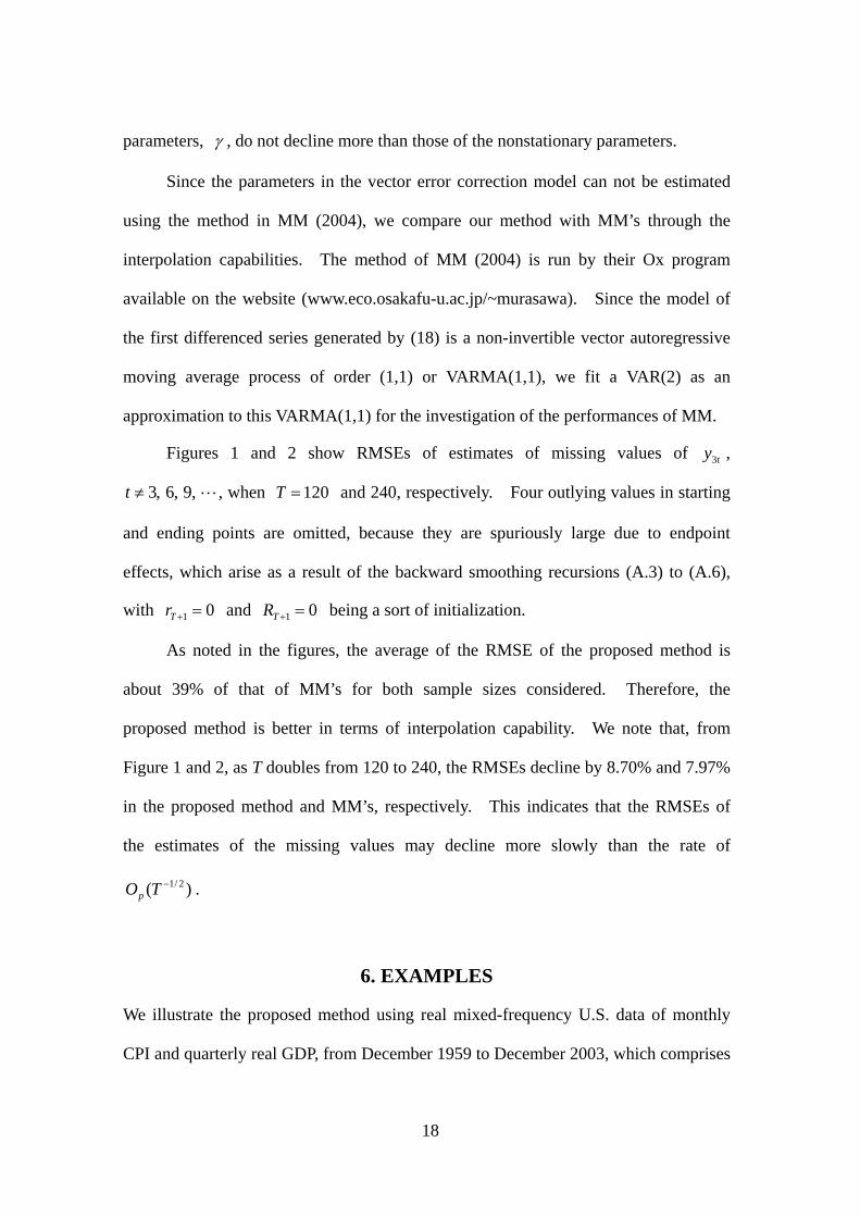
Figures 1 and 2 show RMSEs of estimates of missing values of ,

, when and 240, respectively. Four outlying values in starting

and ending points are omitted, because they are spuriously large due to endpoint

effects, which arise as a result of the backward smoothing recursions (A.3) to (A.6),

with and being a sort of initialization.

ty3

L,9,6,3≠t 120T =

01 =+Tr 01 =+TR

As noted in the figures, the average of the RMSE of the proposed method is

about 39% of that of MM’s for both sample sizes considered. Therefore, the

proposed method is better in terms of interpolation capability. We note that, from

Figure 1 and 2, as T doubles from 120 to 240, the RMSEs decline by 8.70% and 7.97%

in the proposed method and MM’s, respectively. This indicates that the RMSEs of

the estimates of the missing values may decline more slowly than the rate of

. )( 2/1−TOp

6. EXAMPLES

We illustrate the proposed method using real mixed-frequency U.S. data of monthly

CPI and quarterly real GDP, from December 1959 to December 2003, which comprises

18

176 quarters or 529 months of observations. The CPI and GDP data are from the

Bureau of Labor Statistics (www.bls.gov) and from the Bureau of Economic Analysis

(www.bea.gov), are seasonally adjusted, have a base CPI value of 100 in 1982-1984,

and have a unit of GDP in billions of chained 2000 dollars. The original data,

denoted and in month t, were transformed to and by taking

natural logs and subtracting from them the natural logs at the starting dates, as

tCPI tGDP tcpi tgdp

. (19) ⎟⎟⎠

⎞⎜⎜⎝

⎛−−

=⎟⎟⎠

⎞⎜⎜⎝

⎛=

)log()log()log()log(

12:1959

12:1959

GDPGDPCPICPI

gdpcpi

yt

t

t

tt

Henceforth, the lower-case variable names, cpi and gdp, will refer to these

transformations of CPI and GDP.

As mentioned in section 3.2, we first estimate the CI rank and the CI vector by

using a quarterly single-frequency sample, obtained by picking one monthly value of

cpi per quarter and keeping quarterly gdp as is (we call this “skip-sampling”). The

quarterly single-frequency data indicated that the estimated model may have a constant

term. The model selection criteria, minimum AIC and SBC, both indicated choosing

a VAR(4) model. Then, applying Johansen’s trace test to the VAR(4) model,

estimated using the single-frequency data, we obtained a p-value less than 0.001,

which indicated a CI rank of one. The corresponding estimate of the CI vector was

. For the mixed-frequency observations on (1, 2.063)′− ),( ′= ttt gdpcpiy , we

obtained as the estimate of the cointegrating vector by using the

relationship in Pons and Sansó (2005), which we could because GDP is temporally

aggregated of order 3.

(1, 6.189)′−

We used minimum AIC and SBC criteria to select the best monthly (highest

frequency) model, and chose the VAR(4) model

19

( ) 1 10.0900 0.0005 0.4561 0.0008

1, 5.05800.3434 0.0018 0.0993 0.9010t t ty y y− −

−⎛ ⎞ ⎛ ⎞ ⎛ ⎞Δ = + − + Δ⎜ ⎟ ⎜ ⎟ ⎜ ⎟− −⎝ ⎠ ⎝ ⎠ ⎝ ⎠

2 30.2664 0.0054 0.0600 0.00120.0066 0.2126 0.1575 0.0235t ty y tε− −⎛ ⎞ ⎛ ⎞

+ Δ +⎜ ⎟ ⎜ ⎟− − −⎝ ⎠ ⎝ ⎠Δ + ,

0.0432 0.0052ˆvar( )

0.0052 0.0663tε⎛ ⎞

= ⎜ ⎟⎝ ⎠

.

as the best VAR(p) model. For this model, we computed monthly smoothed estimates

of and monthly forecasts of and . tgdp tcpi tgdp

Table 2 shows monthly smoothed estimates of , from 2003:1 to 2003:12, as

examples of monthly smoothed estimates of in the sample period. The

estimates are of high-frequency monthly disaggregated and of low-frequency

quarterly aggregated for 2003. Tables 6 and 7 state out-of-sample (that is, out

of model estimation sample) forecasts of and for 2004 and compare these

with true values. The tables show smaller forecast errors when using mixed-

frequency data than when using single-frequency data. Specifically, the absolute

values of forecast errors are smaller by about 7% and 82% on average.

tgdp

tgdp

tgdp

tgdp

tcpi tgdp

8. CONCLUSION

We have developed and illustrated a method, for estimating a multivariate cointegrated

VAR model with mixed-frequency time-series data, by using a state-space

representation of an error correction model. The method allows us not only to

estimate such a model using mixed-frequency data, but also to estimate missing or

unobserved high-frequency values of the low-frequency variables. Monte Carlo

experiments, applied to mixed-frequency data, with missing observations, and to

single-frequency data, with complete observations, indicate that the proposed method

performs well with missing data due to mixed frequencies.

20

ACKNOWLEDGEMENT

B. Seong’s research was supported by the Korea Research Foundation Grant funded by

the Korean Government (MOEHRD, Basic Research Promotion Fund) (KRF-2007-

331-C00060). S. K. Ahn’s work was supported by the Korea Research Foundation

Grant (KRF-2005-070-C00022) funded by the Korean Government (MOEHRD). P.

Zadrozny is affiliated as a Research Fellow with the Center for Financial Studies,

Goethe University, Frankfurt, Germany, and the Center for Economic Studies and Ifo

Institute for Economic Research (CESifo), Munich, Germany. The paper represents

the authors’ views and does not necessarily represent any official positions of the

Bureau of Labor Statistics.

APPENDIX

Let , and , where

and denote the conditional expectation and conditional

covariance with respect to the density based on .

)|(E += stlst Yxx )|(cov += stl

st YxP )|,(cov 11,

+−− = sttl

stt YxxP

)|(E +⋅ sl Y )|(cov +⋅ sl Y

)(lθWe calculate the prediction and updating recursions using the following

equations (for example, Shumway and Stoffer 1982). For Tt ,,1 L= ,

11

1 −−

− = tt

tt Fxx , , (A.1) GGFFPP t

tt

t ′+′= −−

− 11

1

)( 11 −+− −+= ttttt

tt

tt xHyKxx , , (A.2) 11 −− −= t

tttt

tt

t PHKPP

where . We start iterations (A.1) and (A.2) by setting

and . In order to calculate , and using equations

(A.1) and (A.2), for , we iterate over the backwards recursions

111 )( −−− ′+′′= tttt

tttt

tt QQHPHHPK

λ=00x Λ=0

0P Ttx T

tP TttP 1, −

1,, LTt =

1111 )()( +−+−− ′+−′+′′= tt

ttttttt

ttttt rLxHyQQHPHHr (A.3)

tttttttt

tttt LRLHQQHPHHR 111 )( +

−− ′+′+′′= (A.4)

21

where , , and 01 =+Tr 01 =+TR )( ttst HKIFL −= . Following Durbin and Koopman (2001), we obtain the smoothing equations

tt

ttt

Tt rPxx 11 −− += , , (A.5) 111 −−− −= t

ttt

tt

tT

t PRPPP

for , and Tt ,,1 L=

111,1 )( −+++ −= t

tttt

tsT

tt PLRPIP , (A.6)

for . 1,,1 −= Tt L

REFERENCES

1. Aadland, D. M. (2000), “Distribution and Interpolation Using Transformed Data,”

Journal of Applied Statistics, 27, 141-156.

2. Ahn, S. K., and Reinsel, G. C. (1990), “Estimation for Partially Nonstationary

Multivariate Autoregressive Models,” Journal of the American Statistical

Association, 85, 813-823.

3. Anderson, B. D. A., and Moore, J. B. (1979), Optimal Filtering, Englewood Cliffs,

NJ: Prentice Hall.

4. Bernanke, B. S., Gertler, M., and Watson, M. (1997), “Systematic Monetary Policy

and the Effects of Oil Price Shocks,” Brookings Papers on Economic Activity, 1,

91–157.

5. Brockwell, P. J., and Davis, R. A. (1991), Time Series: Theory and Methods, 2nd

ed., New York: Springer-Verlag.

6. Chen, B., and Zadrozny, P. A. (1998), “An Extended Yule-Walker Method for

Estimating Vector Autoregressive Models with Mixed-Frequency Data,” in

Advances in Econometrics: Messy Data–Missing Observations, Outliers, and

Mixed-Frequency Data, Vol. 13, pp. 47-73, T. B. Fomby and R. C. Hill (eds.),

Greenwich, CT: JAI Press.

22

7. Chow, G. C., and Lin, A. (1971), “Best Linear Unbiased Interpolation, Distribution,

and Extrapolation of Time Series by Related Series,” Review of Economics and

Statistics, 53, 372–375.

8. Cuche, N. A., and Hess, M. K. (2000), “Estimating Monthly GDP in a General

Kalman Filter Framework: Evidence from Switzerland,” Economic & Financial

Modelling, 7, 153–194.

9. De Jong, P. (1989), “Smoothing and Interpolation with the State-Space Model,”

Journal of the American Statistical Association, 84, 1085-1088.

10. Dempster, A. P., Laird, N. M., and Rubin, D. B. (1977), “Maximum Likelihood

from Incomplete Data via the EM Algorithm,” Journal of the Royal Statistical

Society, Series B, 39, 1-38.

11. Durbin, J., and Koopman, S. J. (2001), Time Series Analysis by State Space

Methods, Oxford: Oxford University Press.

12. Engle, R. F., and Granger, C. W. J. (1987), “Co-Integration and Error Correction:

Representation, Estimation, and Testing,” Econometrica, 55, 251-276.

13. Ghysels, E., and Valkanov, R. (2006), “Linear Time Series Processes with Mixed

Data Sampling and MIDAS Regression Models,” Working Paper, UNC and UCSD

14. Granger, C. W. J., and Siklos, P. L. (1995), “Systematic Sampling, Temporal

Aggregation, Seasonal Adjustment, and Cointegration Theory and Evidence,”

Journal of Econometrics, 66, 357-369.

15. Harvey, A. C., and Pierce, R. G. (1984), “Estimating Missing Observations in

Economic Time Series,” Journal of the American Statistical Association, 79, 125-

131.

16. Haug, A. A. (2002), “Temporal Aggregation and the Power of Cointegration Tests:

a Monte Carlo Study,” Oxford Bulletin of Economics and Statistics, 64, 399-412.

23

17. Johansen, S. (1996), Likelihood-Based Inference in Cointegrated Vector

Autoregressive Models, 2nd ed., Oxford: Oxford University Press.

18. Liu, H., and Hall, S. G. (2001), “Creating High-Frequency National Accounts with

State-Space Modeling: a Monte Carlo Experiment,” Journal of Forecasting, 20,

441-449.

19. Marcellino, M. (1999), “Some Consequences of Temporal Aggregation in

Empirical Analysis,” Journal of Business and Economic Statistics, 17, 129–136.

20. Mariano, R. S., and Murasawa, Y. (2003), “A New Coincident Index of Business

Cycles Based on Monthly and Quarterly Series,” Journal of Applied Econometrics,

18, 427-443.

21. Mariano, R. S., and Murasawa, Y. (2004), “Constructing a Coincident Index of

Business Cycles without Assuming a One-Factor Model,” Discussion Paper 2004-

6, College of Economics, Osaka Prefecture University.

22. Mitchell, J., Smith, R. J., Weale, M. R., Wright, S., and Salazar, E. L. (2005), “An

Indicator of Monthly GDP and an Early Estimate of Quarterly GDP growth,” The

Economic Journal, 115, F108–F129.

23. Pons, G., and Sansó, A. (2005), “Estimation of Cointegrating Vectors with Time

Series Measured at Different Periodicity,” Econometric Theory, 21, 735-756.

24. Schweppe, F. C. (1965), “Evaluation of Likelihood Functions for Gaussian

Signals,” IEEE Transactions on Information Theory, IT-4, 294-305.

25. Seong, B., Ahn, S. K., and Zadrozny, P. A. (2007), “Cointegration Analysis with

Mixed-Frequency Data,” CESifo Working Paper Series, No. 1939.

26. Shumway, R. H., and Stoffer, D. S. (1982), “An Approach to Time Series

Smoothing and Forecasting Using the EM Algorithm,” Journal of Time Series

Analysis, 3, 253-264.

24

27. Watson, M. W., and Engle, R. F. (1983), “Alternative Algorithms for the

Estimation of Dynamic Factor, Mimic and Varying Coefficient Regression

Models,” Journal of Econometrics, 23, 385-400.

28. Zadrozny, P. A. (1990), “Estimating a Multivariate ARMA Model with Mixed-

Frequency Data: an Application to Forecasting U.S. GNP at Monthly Intervals,”

Center for Economic Studies Discussion Paper 90-5, Bureau of the Census,

Washington, DC.

25

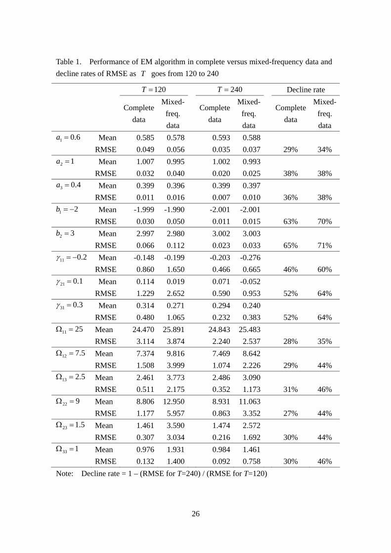
Table 1. Performance of EM algorithm in complete versus mixed-frequency data and decline rates of RMSE as goes from 120 to 240 T

120=T 240=T Decline rate

Complete

data

Mixed-freq. data

Complete data

Mixed- freq. data

Complete data

Mixed- freq. data

6.01 =a Mean 0.585 0.578 0.593 0.588 RMSE 0.049 0.056 0.035 0.037 29% 34%

12 =a Mean 1.007 0.995 1.002 0.993 RMSE 0.032 0.040 0.020 0.025 38% 38%

4.03 =a Mean 0.399 0.396 0.399 0.397 RMSE 0.011 0.016 0.007 0.010 36% 38%

21 −=b Mean -1.999 -1.990 -2.001 -2.001 RMSE 0.030 0.050 0.011 0.015 63% 70%

32 =b Mean 2.997 2.980 3.002 3.003 RMSE 0.066 0.112 0.023 0.033 65% 71%

2.011 −=γ Mean -0.148 -0.199 -0.203 -0.276 RMSE 0.860 1.650 0.466 0.665 46% 60%

1.021 =γ Mean 0.114 0.019 0.071 -0.052 RMSE 1.229 2.652 0.590 0.953 52% 64%

3.031 =γ Mean 0.314 0.271 0.294 0.240 RMSE 0.480 1.065 0.232 0.383 52% 64%

2511 =Ω Mean 24.470 25.891 24.843 25.483 RMSE 3.114 3.874 2.240 2.537 28% 35%

5.712 =Ω Mean 7.374 9.816 7.469 8.642 RMSE 1.508 3.999 1.074 2.226 29% 44%

5.213 =Ω Mean 2.461 3.773 2.486 3.090 RMSE 0.511 2.175 0.352 1.173 31% 46%

922 =Ω Mean 8.806 12.950 8.931 11.063 RMSE 1.177 5.957 0.863 3.352 27% 44%

5.123 =Ω Mean 1.461 3.590 1.474 2.572 RMSE 0.307 3.034 0.216 1.692 30% 44%

133 =Ω Mean 0.976 1.931 0.984 1.461 RMSE 0.132 1.400 0.092 0.758 30% 46% Note: Decline rate = 1 – (RMSE for T=240) / (RMSE for T=120)

26

Table 2. Monthly smoothed estimates of in-sample quarterly , 2003:1 to 2003:12

tgdp

Year: month

Observed Temp. agg.

Skip-sampled

Year: month

ObservedTemp. agg.

Skip-sampled

2003:1 141.58 141.67 2003:7 143.65 144.40 2003:2 141.81 142.11 2003:8 144.20 144.71 2003:3 141.96 141.96 142.12 2003:9 144.76 144.76 145.16 2003:4 142.20 142.37 2003:10 145.06 145.32 2003:5 142.52 143.07 2003:11 145.40 145.72 2003:6 142.97 142.97 143.48 2003:12 145.78 145.78 146.30

Note: Reported “aggregated” and “skip-sampled” in columns 3 and 4, respectively, reflect quarterly sums of monthly values ending in the indicated month and monthly values for that month multiplied by three (in order to be in quarterly form comparable to observed quarterly in column 2).

tgdp

tgdp

Table 3. Monthly out-of-sample forecasts of tcpi

Single-frequency Mixed-frequency Year: month Observed

Forecast Error Forecast Error 2004:1 184.39 184.00 0.39 2004:2 184.71 184.13 0.58 2004:3 185.14 184.05 1.08 184.24 0.90 2004:4 185.35 184.39 0.96 2004:5 185.94 184.51 1.43 2004:6 186.20 184.64 1.56 184.65 1.55 2004:7 186.15 184.79 1.36 2004:8 186.20 184.93 1.27 2004:9 186.36 185.01 1.35 185.07 1.29 2004:10 186.94 185.21 1.73 2004:11 187.20 185.35 1.85 2004:12 187.20 185.39 1.81 185.49 1.71

Note: “Out-of-sample” means for months beyond earlier months, from 1959:12 to 2003:12, used to estimate the model which was used to produce the forecasts.

27

Table 4. Monthly out-of-sample forecasts of quarterly tgdp

Single-frequency Mixed-frequency Year: month

Observed Forecast Error

Forecast Low Freq.

Error Forecast

High Freq.

2004:1 146.133 146.376 2004:2 146.515 146.868 2004:3 146.88 146.51 0.37 146.775 0.10 147.081 2004:4 147.139 147.468 2004:5 147.431 147.744 2004:6 147.69 147.43 0.26 147.767 -0.08 148.089 2004:7 148.074 148.389 2004:8 148.398 148.716 2004:9 148.67 148.17 0.50 148.71 -0.04 149.025 2004:10 149.028 149.343 2004:11 149.34 149.652 2004:12 149.61 148.82 0.79 149.654 -0.05 149.967

Note: Same as in Table 3.

28

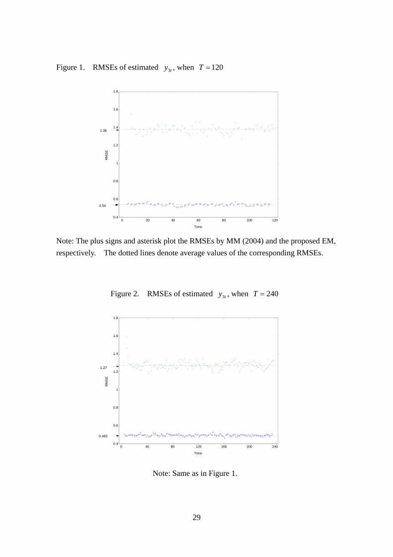
Figure 1. RMSEs of estimated , when ty3 120T =

0 20 40 60 80 100 1200.4

0.6

0.8

1

1.2

1.4

1.6

1.8

Time

RM

SE

1.38

0.54

Note: The plus signs and asterisk plot the RMSEs by MM (2004) and the proposed EM, respectively. The dotted lines denote average values of the corresponding RMSEs.

Figure 2. RMSEs of estimated , when ty3 240T =

0 40 80 120 160 200 2400.4

0.6

0.8

1

1.2

1.4

1.6

1.8

Time

RM

SE

1.27

0.493

Note: Same as in Figure 1.

29