Estimation of the impact of ALMPs on participants' · Web viewTitle Estimation of the impact...
103
Estimating the Impact of Employment Programmes on Participants’ Outcomes M. de Boer Centre for Social Research and Evaluation Te Pokapü Rangahau Arotake Hapori The view and opinions expressed within this report are not necessarily those of the Ministry of Social Development.
-
Upload
trinhkhuong -
Category
Documents
-
view
216 -
download
1
Transcript of Estimation of the impact of ALMPs on participants' · Web viewTitle Estimation of the impact...

Estimating the Impact of Employment Programmes on Participants’ Outcomes
M. de Boer
Centre for Social Research and Evaluation
Te Pokapü Rangahau Arotake Hapori June 2003
The view and opinions expressed within this report are not necessarily those of the Ministry of Social Development.

Table of Contents
ABSTRACT..................................................................................................................4
1 INTRODUCTION.................................................................................................51.1 Employment Evaluation Strategy...............................................................51.2 Consistent and robust estimates of programme impact.............................51.2.1 Structure of report.......................................................................................6
2 PROGRAMME PARTICIPATION............................................................................72.1 Determining programme participation........................................................72.2 Conceptual considerations.........................................................................9
3 NON-PARTICIPANT POPULATION......................................................................133.1 Defining non-participants..........................................................................133.1.1 Inclusion of participants in the non-participant population........................133.1.2 Non-participants subsequent participation in the programme..................133.2 Technical issues in constructing a non-participant population.................143.3 Sampling approach..................................................................................143.4 Alternative samples..................................................................................15
4 JOB SEEKER CHARACTERISTICS......................................................................174.1 Existing observable characteristics..........................................................174.2 Additional dimensions not covered so far.................................................20
5 LABOUR MARKET OUTCOMES..........................................................................215.1 Potential outcome measures....................................................................215.1.1 Stable employment...................................................................................215.2 Current evaluation measures...................................................................215.2.1 Positive labour market outcomes.............................................................225.2.2 Labour market outcomes of job seekers..................................................235.2.3 Work and Income Independence indicator...............................................245.2.4 Potential bias in labour market outcome measure...................................245.3 Enhancing current outcome measures.....................................................265.4 Specification of outcome measures.........................................................275.4.1 Participation start and end dates..............................................................275.4.2 Cumulative versus point in time...............................................................28
6 ESTIMATING THE IMPACT OF PROGRAMMES.....................................................296.1 What is the question?...............................................................................296.1.1 Problem definition: missing data..............................................................306.2 Selection bias...........................................................................................306.3 Some possible estimators........................................................................326.3.1 Key assumptions......................................................................................336.3.2 Simple estimators.....................................................................................336.3.3 Conditioning on observable characteristics..............................................346.3.4 Conditioning on unobservable characteristics..........................................366.3.5 Importance of variable selection...............................................................38
7 PROPENSITY MATCHING..................................................................................397.1 Estimating propensity scores by sub-period.............................................397.1.1 Defining the non-participant population....................................................407.1.2 The problem of common support.............................................................407.1.3 What variables should be included...........................................................427.1.4 Logistic model specification......................................................................437.2 Summary of logistic model.......................................................................447.2.1 Model fit statistics.....................................................................................447.2.2 Variable type 3 effects..............................................................................457.2.3 Distribution of participants and non-participants by propensity score......477.2.4 Balancing test...........................................................................................487.3 Propensity matching.................................................................................52
The view and opinions expressed within this report are not necessarily those of the Ministry of Social Development.

7.3.1 Nearest neighbour matching....................................................................527.3.2 Interval or stratification matching..............................................................537.3.3 Does the matching approach matter?......................................................537.4 Propensity matched estimates of impact..................................................567.4.1 Confidence intervals of estimates............................................................58
8 Conclusions..................................................................................................59
Estimating the impact of programmes on participants’ outcomes
3

Abstract
The report summarises what has been learnt so far in estimating employment programme impact using administrative data in the New Zealand context. The intention is to provide a guide on where this type of analysis might be improved as well as identify issues and risks in the use of administrative data for this purpose. The report covers issues in the definition of programme participation and non-participation, availability of observable characteristics in the administrative data and the specification of a proxy measure of employment outcomes. The report concludes by discussing the general issues involved in estimating programme impact, before detailing the use of propensity matching in estimating the impact of several employment programmes.
Estimating the impact of programmes on participants’ outcomes
4

1 IntroductionThis report is part of a continuing project within the Employment Evaluation Strategy (EES) to provide consistent estimates of the outcomes and impact of employment assistance in New Zealand. The purpose of this work is to compare the effectiveness of different forms of employment assistance in reducing the incidence of long-term unemployment. The present report discusses the technical developments in estimating the impact of employment assistance on participant outcomes.
1.1 Employment Evaluation StrategyThe EES is an interagency project supported by the Ministry of Social Development (MSD) and the Labour Market Policy Group (LMPG) within the Department of Labour. The strategy aims to provide a framework within which interagency capacity building and strategic evaluations sit alongside monitoring employment policies and interventions, and operational evaluation work of individual agencies. Ultimately, the strategy’s goal is to improve the ability of evaluators to provide robust and useful information to those responsible for the policy and delivery of employment assistance in New Zealand.
This strategy was set up in 1999 and arose through a review by the Department of Labour of employment evaluations undertaken to identify successful policies, interventions and service delivery options [G5 10/10/97 refers]. The review found that past evaluations were limited in their ability to inform future employment policy because of their focus on single interventions and lack of comparability [STR (98) 223 refers].
The components of the EES are as follows:
building evaluation capacity in the immediate future
addressing a key question, "what works for whom and under what circumstances?”
wider strategic issues, such as the community benefits associated with employment interventions.
This paper addresses the first of these goals, by providing a summary of current knowledge in the estimation of programme impact on participants’ outcomes.
1.2 Consistent and robust estimates of programme impactOne goal of EES is to provide consistent estimates of the effectiveness of employment programmes. While an apparently simple goal, it is difficult to address, primarily because of the need to know the effect that employment programmes have on non-participants as well as on participants (Calmfors 1994; Chapple 1997; de Boer 2003a). Instead, most evaluations in New Zealand and overseas only focus on one part of this question: the impact that programmes have on participants’ outcomes. It is this narrower question that the following paper examines in the New Zealand context, specifically to be able to:
identify programme participants and non-participants
determine the labour market outcomes of the two groups
estimate the impact of programmes on participants’ outcomes.
The intention is to document achievements so far, to avoid the duplication of effort, and to identify areas for further improvement.
Estimating the impact of programmes on participants’ outcomes
5

1.2.1 Structure of report
This report is in five parts, each corresponding to the key components of any analysis of programme impact. These are:
identification of programme participants
definition of non-participants
characteristics of participants and non-participants
labour market outcomes
estimation of impact on outcomes.
The basic approach will be to introduce each topic and place it within the New Zealand context. This is followed by a summary of what has been done so far, and what issues have arisen and the solutions or limitations that they impose. This is illustrated with examples from recent analysis of programme impact, with the primary example being the recent review of the effectiveness of several different types of employment programmes (de Boer 2003a). Each section concludes with outstanding issues and possible avenues for further work.
Estimating the impact of programmes on participants’ outcomes
6

2 Programme participationThe most basic element of any analysis of programme impact is to differentiate those people who participated in the programme of interest, and when, from those who did not. Whilst the definition and identification of programme participants appears to be a trivial issue, there are several conceptual as well as technical considerations. In particular, what constitutes programme participation (for example, when a person is only on the programme for a short while) as well as the confidence that the evaluator has in the accuracy of this information in the administrative data.
2.1 Determining programme participationRecording of participation in employment programmes in the MSD administrative databases is complex, in part because the administration of programmes occurs in more than one administrative system (eg SOLO and SWIFTT) and across more than one government agency (eg Work and Income (Work and Income) versus Tertiary Education Commission1 (TEC)). This requires a number of assumptions in the interpretation of the data.
The employment database (SOLO) provides most information on programme participation, with income database (SWIFTT) information supplementing this for two programmes (Work Start Grant and Training Incentive Allowance), while TEC provides further information on Training Opportunities participants. In addition, a contracting database is also coming into operation (2002/03) that will complement the information recorded in SOLO on those employment programmes contracted at the regional level.
The extraction of participation information requires detailed knowledge of the database structures as well as a good institutional knowledge of the programmes themselves.2 This paper will not cover the technical issues with obtaining participation records, and will instead cover some of the higher level issues that evaluation analysts will need to deal with once this information has been obtained.
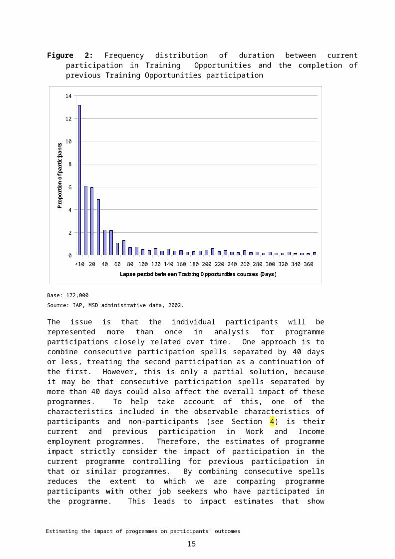
What type of programme is it?One important problem with administrative data on programme participation is knowing what the form of assistance the participant received. Often programmes are recorded by their name (eg Job Plus, Work Action, Access) and it is often not possible to know the nature of these programmes (eg wage subsidy, intensive case management or training), as much of this documentation sits outside the administrative system. This is most problematic for locally developed programmes (regional initiatives), which are aggregated under very general headings in the administrative database. Even nationally prescribed and established programmes, such as Training Opportunities, it is not always possible to tell in any detail about the assistance given. In the case of Training Opportunities, TEC contract a variety of programmes from basic literacy to specialised vocational services. However, it is not possible to differentiate between these types of training using MSD administrative data, although further information is available on the TEC database.
When did the participation finish?When a case manager makes a successful referral to a programme, they normally enter a start date. However, because case managers do not always know the 1 Formally Skill New Zealand.2 The technical process for consistently extracting participation information is being developed through the IAP
Business Rules process.
Estimating the impact of programmes on participants’ outcomes
7

outcome of they do not necessarily enter an end date. End dates are complicated further for client placements (mainly subsidy-based programmes), as the contract has both an expected end date and an actual end date. If the end date field remains null four months after the last claim against the contract or four months after the expected end date of the contract, then the expected end date populates the actual end date; this affects 56% of contracts. It appears that contracts are running for their full term while payment information shows the contract had run for less than this.
The response to this problem was to estimate end dates based on observed and expected benchmarks. For contract client placements, it was possible to base the end date on the expected duration of the placement, the commitment over this period and the actual amount paid for the contract. Based on the assumption the commitment was spread evenly over the duration of the contract, the end date was based on the duration of the contract times the ratio between the commitment and the total amount claimed. Therefore, for exhausted commitments the calculated end date will be the same as the expected end date. Conversely, if no claims were made against the contract then the calculated end date would be equal to the start date. The calculated end date replaces all contract end dates.
For participation records it was more difficult to estimate the duration of the placement; therefore, the estimated end dates for participations are less accurate than for contract client placements. Missing participation end dates (12% of total participations3) were calculated on a fixed duration for the employment programme in question. Where end dates exist for at least 100 participants in a given programme, the average duration of that intervention was calculated. Where there were not enough end dates to calculate the average duration for a programme, then duration was estimated based on how long the participation should have taken (affected 0.01% of participations). Sometimes this information was available through programme documentation; otherwise, duration of similar interventions was used.
How much did it cost?As the above suggests, there is also considerable variability in the accuracy of information on the cost of different interventions. For those funded through the Subsidised Work Appropriation and administered through SWIFTT it is possible to gain accurate individual level information on the cost of interventions. However, for the majority of interventions, at best it is possible to know the average per participant cost, while at worst there is no clear information on the contract cost nor the per-participant costs. This latter category is comprised of the locally contracted programmes, in which contract information is paper-based and exists outside the administrative databases.
3 Excluding contract client placements.
Estimating the impact of programmes on participants’ outcomes
8

SummarySource Programmes Data Quality CommentsContract client placements
Job Plus, Community TaskForce, Community Work, Activity in the Community, TaskForce Green, Job Connection, Enterprise Allowance
Good information on type, duration and cost of programmes.
Tertiary Education Commission
Training Opportunities Good information on duration and date of spells, but limited data on nature of training or cost.
Locally contracted programmes
Generic – job search, work confidence, work experience, seminars.
Inconsistent and variable quality information on all dimensions – programme type, duration participants and cost.
Introduction of Conquest may improve the quality of information on this type of assistance.
Further enhancementsThe quality of information on programme participants depends on available data structures in which to enter programme information and the degree to which front line staff are trained and willing to enter this information accurately and fully. The experience with a number of programmes, especially those delivered locally, is that administrative data often only partially represents what has happened on the ground. For example, people can be recorded as having participated when they did not participate or may have participated in an entirely different programme
Work has been undertaken by the MSD national contract team to resolve some of these issues, in particular by developing contract management system (called Conquest) to track contracts for locally delivered programmes. This system is maintained by a relatively small number of people and therefore it is hoped that the information will be more complete and accurate than what is currently available.
2.2 Conceptual considerationsAlongside the technical issues of defining participation, there are also a number of conceptual considerations. One of the most common is defining what constitutes as a sufficient participation spell for the programme to have a meaningful effect. There are two possible approaches. The first is to ignore the problem and simply state that the impact estimate is for everyone who started the programme irrespective of their subsequent programme duration. This is appealing for its simplicity and avoids making any arbitrary decisions about the minimum cut-off before the duration on the spell is counted. The limitation of this approach is that it under-estimates programme effect by including people who did not experience the programme effect. The alternative is to examine the actual distribution of programme durations and make some judgement over the appropriateness of including spells of relatively short duration, given the overall distribution of spells.
Estimating the impact of programmes on participants’ outcomes
9
The choice of strategy depends on the assumed effect of the programme relative to its duration. For example, Figure 1 shows the frequency distribution of the duration of all recorded Training Opportunities participations on the MSD administrative databases. In general, most participation spells lasted for between 20 and 180 days, with only a small proportion going for more than six months (9,740/7.8%). At the other extreme, a small proportion spent less than 10 days on the programme (3,549/2.8%). The decision in this example was to exclude participations that lasted for a week or less.
If duration is thought to be an important factor in determining programme impact, it may be useful to divide participants accordingly (eg 0-1 month, 1-3 months, and 3+ months) and estimate impact for each of these groups separately. This provides a more detailed analysis of the influence of programme duration on the “locking-in effect” of the programme as well as the impact on outcomes with respect to the time spent on the programme.
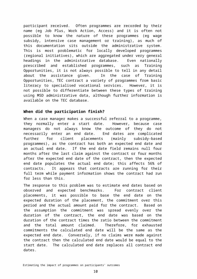
A further consideration is multiple participations in the same programme. In a number of cases, it is common to see a person to participate in the same programme several times in rapid succession. Using Training Opportunities as an example, Figure 2 shows the distribution of spells between successive Training Opportunity courses. Not shown in the figure are just over 50% of participants who did not have a successive spell on Training Opportunities. What is notable from the frequency distribution is that approximately 30% of participants started another Training Opportunities course within 40 days of completing one.
Figure 1: Frequency distribution of the recorded duration of job seekers’ participation in
Training Opportunities
0
2
4
6
8
10
12
<10 20 50 80 110 140 170 200 230 260 290 320 350
Programme Duration (Days)
Prop
ortio
n of
par
ticip
ants
Base: 125,600
Source: IAP, MSD administrative data, 2002.
Estimating the impact of programmes on participants’ outcomes
10

The issue is that the individual participants will be represented more than once in analysis for programme participations closely related over time. One approach is to combine consecutive participation spells separated by 40 days or less, treating the second participation as a continuation of the first. However, this is only a partial solution, because it may be that consecutive participation spells separated by more than 40 days could also affect the overall impact of these programmes. To help take account of this, one of the characteristics included in the observable characteristics of participants and non-participants (see Section 4) is their current and previous participation in Work and Income employment programmes. Therefore, the estimates of programme impact strictly consider the impact of participation in the current programme controlling for previous participation in that or similar programmes. By combining consecutive spells reduces the extent to which we are comparing programme participants with other job seekers who have participated in the programme. This leads to impact estimates that show principally the effect of participating over not participating, rather than the marginal effect of additional time spent participating in a programme.4
The challenge in interpreting the findings with respect to multiple programme participations is well illustrated with respect to Training Opportunities. In the two years leading up to participation in a Training Opportunities, participants spent an average of 43 days in training, with 19% in training in the previous quarter, and 21% 4 This does not exclude estimating the effect of participation duration on programme impact. Moreover, from a policy
perspective, such estimates would be very valuable in determining operational parameters (eg does programme effect occur in the initial participation period while longer spells have little additional benefit?).
Figure 2: Frequency distribution of duration between current participation in Training Opportunities and the completion of previous Training Opportunities participation
0
2
4
6
8
10
12
14
<10 20 40 60 80 100 120 140 160 180 200 220 240 260 280 300 320 340 360
Lapse period between Training Opportunities courses (Days)
Prop
ortio
n of
par
ticip
ants
Base: 172,000
Source: IAP, MSD administrative data, 2002.
Estimating the impact of programmes on participants’ outcomes
11

in the quarter prior to that. This means that any impact estimate is of the effect that the additional training (over and above the previous 43 days) on outcomes, rather than the impact of Training Opportunities compared to not participating. When multiple participations are a common feature of a programme, such as Training Opportunities, it may be worthwhile to analyse programme participation according to the number of participations. One specification may be to analyse the impact of the very first participation spell, the second participation spell and so on. An alternative would be to define total duration on Training Opportunities over a given interval (eg two years) and categorise total programme durations.
Estimating the impact of programmes on participants’ outcomes
12

3 Non-participant populationOnce the participant population is defined, the next question is how to define the non-participant population. Most measures of programme impact discussed in Section 6.3 rely on information on the characteristics and outcomes of non-participants. Like the definition of the participants, defining the non-participant population raises several conceptual and technical challenges.
3.1 Defining non-participantsOn the face of it, non-participants are the binary opposite of participants. However, participants do not participate in the programme all the time, and therefore there will be considerable periods of time when a given participant will be a non-participant. Conversely, non-participants may not necessarily participate in the evaluated programme; however, they do continue to participate in a range of activities, both known and unknown to the evaluator. The treatment of participants and non-participants determines the parameter estimated in the analysis. So far there are two key issues to consider; the way they are resolved remains an issue for debate; the solutions proposed here are only partial.
3.1.1 Inclusion of participants in the non-participant population
One decision is the treatment of those non-participants who have previously participated in the evaluated programme, or, by extension, in similar programmes. One direct approach is to exclude them from the analysis, which sets up any comparison group to comprise of people who have not participated in the programme before their selection. The problem this poses is the arbitrary nature of the exclusion period (one, two or three years prior to their selection into the non-participant population) as well as what programmes justify exclusion from the non-participant group.
The second solution currently favoured is to only exclude from the non-participant population those participants included in the analysis. This means that a certain proportion of the non-participant population will be previous participants in the programme. Therefore, impact estimates will reflect the effect of participation over and above a baseline level of participation in the employment programme (including the latent effects of those who participated in the programme in the past).
3.1.2 Non-participants subsequent participation in the programme
The converse scenario is the participation by non-participants in the programme after their selection into the non-participant sample. Again, these participants could be excluded from the non-participant population, raising the same issues over which time frame and which programmes on which to base the exclusion. In addition, this would violate the principle of only using information on participants and non-participants available at the time of their selection to the programme.
For these reasons, the following analysis takes the approach of retaining such “future participants” in the non-participant sample. The implication will be that a certain proportion of the non-participant population will experience the benefits or costs associated with participation in the programme or similar programmes at some unspecified future time.
This problem is common to experimental designs, where often a significant proportion of the control group participates in the programme or very similar programmes (Heckman, LaLonde and Smith 1999). In their review of social experiments, Heckman et al (1999) found that between 5% and 36% of participants dropped out of
Estimating the impact of programmes on participants’ outcomes
13

the evaluated programme, whilst between 3% and 55% of the control group participated in the programme or close substitutes. These studies normally adjust their impact estimates to take account of the contamination of the non-participant population, usually in conjunction with drop out amongst non-participants. The procedure is a variant of the latent variable estimator:
TT = E(Y1|Z1) – E(Y0|Z0)
Pr(D=1|Z1) – Pr(D=1|Z0)
where Y1 = outcomes achieved by participants
Y0 = outcomes achieved by non-participants
D = Programme participation (D = 1) or non-participant group (D = 0)
Z1 = dummy variable for membership of the participant group
Z0 = dummy variable for membership of the control group.
The basic principle is that the “true” estimate of the impact on the treated is the difference in outcomes between the original participant and control group adjusted by the relative proportions of each group who participate in the programme. However, in the case of experimental designs, this requires the assumption that assignment to the participant and control groups has no impact on either participation or outcomes for those people who do not subsequently participate in the programme.
While a possible advancement on the current analysis, the adjustment has not been used in the work conducted so far. However, it may be worthwhile to include it as a diagnostic check, that is, show the proportion of non-participants previously participating the in the programme as well as the proportion of non-participants who subsequently participate after selection into the comparison group.
3.2 Technical issues in constructing a non-participant populationAt any one time, the MSD administrative data contains more than 500,000 active working-age benefit recipients and job seekers. It is not practical to use information on all these people in estimating the impact of employment programmes. Therefore, the analysis of the programme effectiveness is based on randomly selected samples of this population. These samples are used to estimate the impact of any number of programmes using alternative estimation techniques. This is for practical convenience, namely to reduce the amount of disk space used in doing this work, as the alternative would be to generate multiple sample populations for each individual analysis.
3.3 Sampling approachThe sample population is defined as all people receiving a core benefit for more than one day in each calendar quarter.5 The samples for each quarter population are drawn independently, so that a given person may be selected more than once in different quarter periods. This is to simplify the process of extending the sample over time, in that new quarter periods can be drawn without having to re-draw samples for previous periods. A further point to note is that multiple selection of non-participants in different quarters does not mean a duplication of information due to the presence of time variant characteristics (eg age, benefit duration and participation in employment programmes).
After identifying all active beneficiaries in each quarter, the next step was to determine a random date within the spell(s) they were on the benefit within the
5 This approach was first developed by Maré (2000).
Estimating the impact of programmes on participants’ outcomes
14
specified quarter (as illustrated in Figure 3).6 This was achieved by multiplying the total spell duration for each individual within the quarter with a random variable with a uniform density function, between 0 and 1. This reduced duration value was then added to the start of the individual’s first spell within the quarter (either actual spell start date or quarter start date depending which comes later). If there are multiple spells within the quarter, then, if the reduced duration exceeded the duration of the first spell, the remainder of the reduced duration was added to the start of the second spell and so on (see Figure 3). This meant that all beneficiaries active within the quarter could be included and that that their selection date fell within a period they were active on the benefit.
The above procedure was favoured over simple stock selection7 for two reasons. The first is that simple stock selection is biased towards job seekers with longer duration spells and therefore does not represent the beneficiary population fully. Secondly, this selection process simulates the distribution of job seeker start dates over the quarter is similar to the distribution of participation start dates (ie not all participation start dates occur on a single day in the middle of the quarter).
3.4 Alternative samplesThe beneficiary population is quite heterogeneous from unemployed people with very short periods of benefit receipt through to Invalids beneficiaries, who can spend many years on benefit. Conversely, employment programmes can be targeted at quite specific groups of people (eg based on ethnicity or unemployment duration). For this reason a number of different samples are drawn for each quarter period, to accommodate the need to select non-participants with specific characteristics.
6 Remember that the beneficiary sample include all those active within the quarter not simply those who may have start a benefit spell within this period.
7 Selecting all beneficiers active on the benefit on a given day.
Figure 3: Hypothetical example of selecting a random date for comparison job seekers.
Time
Specific study period
Benefit duration85 days 78 days60 days
Study period duration= 115 days30 days 60 days 25 days
Random value = 0.6
Random duration = 55 days 30 days 25 days
Random date
x
Estimating the impact of programmes on participants’ outcomes
15

Main random sampleThe largest sample is a random selection of 20,000 beneficiaries within each quarter who are registered as seeking employment. This population is used for estimators that require random sample populations.
Choice-based samplesAfter this random sample is selected, a number of sub samples are drawn from the remaining benefit population in the quarter, unlike the main random sample; each sub-sample is drawn from the main population and then returned for the next sub-sample selection. In other words, while no one from the random sample will be in the sub-samples, people may be in more than one sub-sample. In cases where samples are combined, then multiple instances of the same client are removed.
To date, these sub-samples have been used in constructing propensity matched non-participant groups, where the participants are drawn from specific sub-populations that are not well represented among the general beneficiary population (see Section 7.1.2). Currently selected sub-samples include:
Maori
Pacific
teen (under 20 years)
youth (under 25 years)
short-term beneficiaries (<26 weeks)
long-term beneficiaries (26+ weeks)
extra long-term beneficiaries (204+ weeks)
current participation in employment programmes
previous participation in employment programmes
previous participation in training programmes.
Estimating the impact of programmes on participants’ outcomes
16

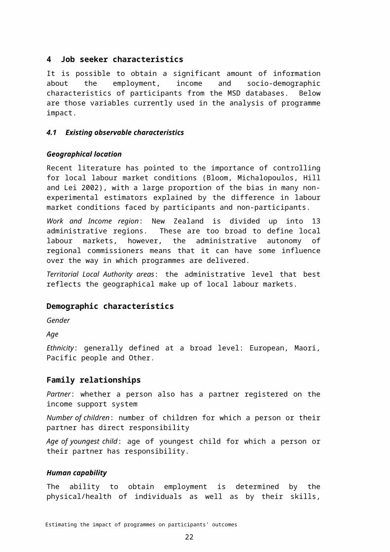
4 Job seeker characteristicsIt is possible to obtain a significant amount of information about the employment, income and socio-demographic characteristics of participants from the MSD databases. Below are those variables currently used in the analysis of programme impact.
4.1 Existing observable characteristics
Geographical locationRecent literature has pointed to the importance of controlling for local labour market conditions (Bloom, Michalopoulos, Hill and Lei 2002), with a large proportion of the bias in many non-experimental estimators explained by the difference in labour market conditions faced by participants and non-participants.
Work and Income region: New Zealand is divided up into 13 administrative regions. These are too broad to define local labour markets, however, the administrative autonomy of regional commissioners means that it can have some influence over the way in which programmes are delivered.
Territorial Local Authority areas: the administrative level that best reflects the geographical make up of local labour markets.
Demographic characteristicsGender
Age
Ethnicity: generally defined at a broad level: European, Maori, Pacific people and Other.
Family relationshipsPartner: whether a person also has a partner registered on the income support system
Number of children: number of children for which a person or their partner has direct responsibility
Age of youngest child: age of youngest child for which a person or their partner has responsibility.
Human capabilityThe ability to obtain employment is determined by the physical/health of individuals as well as by their skills, experience and qualifications to undertake different types of employment. In addition, indicators of human capability are often used to target or determine eligibility for employment assistance.
Education qualifications: highest educational qualification achieved. This is generally recorded at start of each unemployment spell and may not be updated on a regular basis.
Service group indicator (SGI): SGI was the MSD’s risk assessment tool derived from several weighted socio-demographic and attitudinal responses. From a continuous point score job seekers are classified into one of five groups (SGI 1 to 5): 1 being highly employable, through to 5, meaning severely disadvantaged. An extra SGI of 0
Estimating the impact of programmes on participants’ outcomes
17

was added for those not formally assessed but considered by case managers to be equivalent to SGI 1 job seekers.
Ministerial eligibility: a number of criteria are available to case managers to enable them to refer job seekers who are unemployed for less than 26 weeks but who are considered “at risk” of long term unemployment. These criteria were formalised into the broad heading of Ministerial Eligibility in July 1999.
Criminal conviction: job seekers who are known to have spent time in prison
Alcohol and drug: any identified alcohol or drug problems
Literacy problem: case manager record whether a job seeker has a literacy, numeracy or language barrier
Physical disability: any identified physical disability
Mental disability: any identified mental disability
Intellectual disability: any identified intellectual disability
Sensory disability: any identified sensory disability
Disability: any one of the identified disability types.
Benefit type: Based on the benefit that a person was receiving at or before the start date. Provides information on the probability of moving into employment as well as the likelihood of receiving employment assistance; for example, little employment assistance is targeted to Invalids and Sickness beneficiaries.
Programme participationAs discussed in the sections regarding the selection of participants and non-participants, it is important to control for the previous and current participation in employment programmes. Two measures have been developed for this purpose: the first measures the number of days in the two years prior to participation start date or date of selection into the non-participants sample on different types of employment programmes. The second, a simple dummy variable, is whether the person was on any programme within a month of their selection/participation start date.
There are eight broad groupings of employment programmes:
Any programme: participation in any employment programme
Wage subsidy: wage subsidy programmes in the for-profit sector or self-employment assistance
Training: participation in a training programme (primarily Training Opportunities)
Work confidence: assistance to provide people with the confidence and self-esteem to look and undertake employment
Work experience: placements in private, government and community organisations to gain experience of employment and habits
Job search skills: assistance to enable job seekers to identify employment more effectively
Into work: assistance given to enable people to transition from benefit into employment
Information services: help people identify suitable career and employment aspirations
Other: programmes that do not fit any of the above classifications.
Estimating the impact of programmes on participants’ outcomes
18

Benefit and unemployment historyThe duration of current unemployment spell is a good predictor of likely ongoing unemployment. Three measures were used to capture historical information on income support and employment histories.
Current register duration: official measure of unemployment duration and cumulates register spells separated by intervals off the register of no more than three months. This is often used to determine eligibility for employment programmes (eg more than six months registered unemployed).
Current benefit duration: measured in the same way as unemployment register duration; however, the separation between individual benefit spells can be no more than two weeks. Enables the capture of information on benefit spells that does not require the person to be registered unemployed.
Current Work and Income contact duration: composite of register, benefit and programme participation information and calculates duration across spells separated by less than three months.
In addition to the current spell of unemployment/benefit receipt, three complementary measures determine the total time on register, benefit, Work and Income contact over the previous five years from selection/participation start date.
Cumulative register duration: proportion of last five years on unemployment register.
Cumulative benefit duration: proportion of last five years receiving any type of core benefit assistance (excludes second- and third-tier assistance).
Cumulative Work and Income contact duration: proportion of last five years on register, benefit or participating in employment programmes.
Sequence of Work and Income historyIn addition to looking at total time in different states, a further time series measure was used to categorise the activities of people with respect to Work and Income services in quarterly periods over the two years leading up to selection/participation start date. In each quarter the amount of time spent in each of the states is calculated. Where there is a participation in an employment programme then the longest time spent on any one programme is the state recorded for that period. In all other cases, it is the longest period spent in any non-employment programme state.
dependent on income support
independent of income support
participating in a wage subsidy programme
participating in a training programme
participating in a work experience programme
participating in a work confidence programme
participating in a job search programme
participating in other programme type.
Estimating the impact of programmes on participants’ outcomes
19

4.2 Additional dimensions not covered so far
Previous work experienceThe nature of previous work may provide additional information on the possible employment opportunities available to job seekers. This dimension is approximated by the time that people are independent of Work and Income assistance, but this provides no information on what they might have been doing while independent of Work and Income assistance. However, it is possible to augment this with information in SWIFTT with respect to previous activity before moving onto a benefit as well as from SOLO through preferred job choices. This could be used to get some indication of what type of skill level or industry the job seeker is attempting to access.
Income historyLack of information on income is the most significant gap in the observable characteristics of participants and non-participants. This information would be most important for measures based on controlling for observed characteristics with respect to people’s employment outcomes. Techniques that are based on matching participants and observably similar participants are probably less affected, given that previous income is not a direct consideration in participation decisions (it is not part of any eligibility criteria and is unknown to the case manager).
MotivationDifficult to observe characteristics as motivation, self-esteem and ability are not included in the current analysis. Some of these dimensions are covered by the SGI questionnaire and could be represented independently of the overall score. However, these are single-question responses and therefore would only provide a limited view on these complex concepts.
Estimating the impact of programmes on participants’ outcomes
20

5 Labour market outcomesA measure of outcomes is key to assessing the effectiveness of employment programmes and one that was most difficult to make successfully, as will be discussed below. Moreover, although official MSD measures exist, their limits prevent their use for this type of analysis.
5.1 Potential outcome measuresSeveral types of outcome exist in the literature; in general, US studies have tended to use total income, while the European literature the tendency has been to look at labour market outcomes (Heckman, LaLonde and Smith 1999). New Zealand can be characterised as focusing on labour market outcomes rather than income estimates. However, within this broad categorisation, there exists a considerable range of measures, a variety that in part comes from the particular perspectives of the evaluations themselves as well as the information available. In this respect, New Zealand is no exception, with outcome measures strongly influenced by current reliance on MSD administrative data.
5.1.1 Stable employment
Stable employment (SE) is the official measure to assess the outcomes of its employment programmes. The definition of stable employment is as follows:
job seeker enrolled as unemployed for more than six months
job seeker placed into employment within eight weeks of completing an employment programme
job seeker remains off the unemployment register for more than three months.
The limitations of this measure are:
outcomes other than employment are not included
it is only able to identify outcomes achieved over a fixed period (within eight weeks of programme completion)
it is based on SOLO information only, excluding more reliable benefit (SWIFTT) data on labour market outcomes
under-reporting of SE is also likely because case managers do not always enter programme end dates into SOLO, so it is not possible to calculate SE outcomes.
5.2 Current evaluation measuresFor these reasons evaluations of employment programmes rely on alternative outcome measures. The two developed to date brought together the strengths of the two MSD databases (SWIFTT and SOLO) and were able to include a more comprehensive range of outcomes (eg training) and flexible measurement periods. This flexibility allowed the analysis to consider different outcomes for individual programmes and to tailor them to answer specific research questions.
Estimating the impact of programmes on participants’ outcomes
21
5.2.1 Positive labour market outcomes
The labour market outcome measure draws together three different histories of individual job seekers – benefit, register and programme participation. Interleaving these histories produces a continuous history of the type of assistance job seekers receive and identifies the types of outcome achieved when they no longer require this assistance. Figure 4 provides a stylised example of such a history; it shows the parallel spells that a job seeker has spent on the benefit, register and programmes and the defined labour market outcome history over this period. Benefit information was the main determinant of labour market status. In the example, while on the unemployment benefit, the job seeker was unemployed, but once they move onto the sickness benefit their status becomes “left the labour market’. Use of register history occurs only where there was no benefit history available for the job seeker within the
report period. This was because SWIFTT data is considered to provide a more complete picture of job seeker status while in contact with the MSD and the reasons for exiting (lapsing). This was particularly true for data prior to October 1998, when the two databases were operated independently of each other.
Whist SWIFTT benefit information forms the base for the outcome measure, programme participation was always favoured over either register or benefit history. This was to capture any interventions received by job seekers over the period in question. Using the example in Figure 4, while the lapse reason from the benefit states the person has moved into full-time work, it can be seen that this was initially as part of wage subsidy programme. Accordingly, during the subsidy period, the job seeker’s labour market status was subsidised employment. Once the subsidy has ended and if the job seeker has not come back into contact with the MSD, the assumption is that they are in unsubsidised employment.
Figure 4: Stylised history of benefit, register and programme participation and resulting outcome history.
Programme Wage Subsidy
Outcome
Register UnemploymentDNC
Unemployment
Unemployment Subsidised full-time work
Unsubsidised full-time work
Unemployment Left labour market
Time
SicknessUnemploymentUnemploymentFull time work
Benefit
Estimating the impact of programmes on participants’ outcomes
22

The labour market outcome measure defines people as being in a number of different states:
Unemployed: receiving unemployment or related benefit
Work and Income programmes: participating in employment programmes excluding training and wage-subsidy/self-employment assistance
Training: participation in Work and Income training programme or having a lapse explanation that suggests they have decided to take up independent study
Subsidised full time employment: receiving a wage subsidy while in employment or receiving assistance in setting up an independent firm
Unsubsidised full time employment: left the benefit with a lapse reason of employment.
Left the labour market: have a lapse reason that indicates an exit to a non-employment or to training
Miscellaneous: no longer receiving income or employment assistance and where the type of outcome the participant achieved is unknown.
5.2.2 Labour market outcomes of job seekers
Figure 5: Labour market outcomes of Training Opportunities participants 1 year prior to participation start and five years afterwards
0%
10%
20%
30%
40%
50%
60%
70%
80%
90%
100%
Lapse period after participation start date (months)
Pro
porti
on o
f job
see
kers
(%)
Unemployed 43% 57% 0% 45% 48% 45% 43% 40% 39% 35% 34% 32% 31%
Unsubsidised Employment 6% 4% 0% 8% 14% 17% 19% 21% 22% 22% 23% 24% 25%
Subsidised Employment 1% 1% 0% 4% 3% 2% 2% 2% 1% 1% 1% 1% 1%
Training 7% 9% 100% 28% 14% 11% 9% 9% 8% 7% 7% 6% 6%
Left Labour Market 9% 9% 0% 6% 9% 10% 11% 12% 13% 14% 15% 16% 17%
Miscellaneous 34% 20% 0% 8% 10% 14% 14% 14% 16% 18% 18% 20% 19%
Emp Programmes 1% 2% 0% 2% 2% 2% 2% 2% 2% 2% 2% 1% 1%
-12 -6 0 6 12 18 24 30 36 42 48 54 60
Source: Information Analysis Platform, MSD 2002
Estimating the impact of programmes on participants’ outcomes
23

Figure 5 shows the outcomes achieved by Training Opportunities participants over a six-year period, one year before participation start and five years afterward. The inclusion of pre-participation outcomes helps to gain a sense of what participants are doing before starting a given programme. In this instance a large proportion of Training Opportunities participants have had some form of previous training as well as go on to have further training. In both cases, it is highly likely that this involves other Training Opportunities courses (see Section 2.2). This helps gives the analyst some guidance a over what variables may be important in subsequent analysis; in this instance, the likely importance of previous training as well as the role of subsequent training on outcomes.
For reasons discussed below this measure has been rejected as an unbiased outcome measure and is only used to illustrate participants’ possible outcomes, but should not be used in the estimation of programme impact on outcomes.
5.2.3 Work and Income Independence indicator
The second outcome measure, and the one favoured in this analysis, determines whether a person was independent of Work and Income assistance.8 In this case, independence means that they are no longer receiving any income or employment assistance from Work and Income. This includes receiving a core benefit, participating in a specific employment programme or being actively case managed. The current measure was not able to capture the latter form of assistance, but should be able to do so in the future. Therefore, if a person was not receiving a core benefit and not participating in an employment programme they were considered independent of Work and Income assistance.
However, there are some grey areas in the definition. People receiving supplementary income but no core benefit are still defined as independent of Work and Income assistance. For those job seekers receiving no income assistance over the study period but are registered unemployed, then their register status replaces benefit status as a measure of independence of Work and Income assistance.
The measure is attractive for its simplicity, both in its conception and in construction. However, it does not fully capture the intended outcomes of an employment programme. For example, independence of Work and Income assistance was usually because the job seeker gains employment, but there are also other reasons: prison, death, emigration or a partner gaining employment. Likewise, those still dependent on Work and Income assistance may be participating in further training or other forms of assistance that are legitimate positive outcomes for certain programmes.
5.2.4 Potential bias in labour market outcome measure
The reason for favouring Work and Income independence over the labour market outcome measure is the potential bias in the latter. Specifically, it is thought that programme participants are more likely to have lapse reasons recorded and therefore have higher positive outcomes such as unsubsidised employment relative to non-participants. This problem was most clearly illustrated in the evaluation of the Work Track programme (de Boer 2003b) where recent analysis of its impact contradicted the findings of the initial evaluation (Swindells 2000). While a number of factors
8 Maré (2000) in his analysis of the impact of New Zealand employment programmes developed a similar measure that relied on SOLO register instead of SWIFTT benefit status. The independence of W&I measure is favoured in this instance as it is able to capture a broader set of outcomes. In particular, register status only includes people registered as unemployed, if they move onto non-work tested benefits then they move off the register and is a positive outcome in terms of Maré’s measure. However, while more comprehensive, the independence of W&I measure is subject to the same criticism, as leaving W&I assistance can be associated with both negative as well as positive outcomes for the individual.
Estimating the impact of programmes on participants’ outcomes
24

where identified, one reason was the use of the labour market measure in the initial evaluation and the independence of Work and Income measure in the re-analysis.
The contrast between the two measures (independence of Work and Income and unsubsidised work) is given in Figure 6 for Work Track participants. This clearly shows the number of participants recorded in unsubsidised employment is only a subset of all participants who become independent of Work and Income assistance. Those participants with miscellaneous outcomes largely explain the difference between the two measures.
While not a significant issue in itself, the problem arises from the inconsistencies in the recorded accuracy of these benefit exits. As Figure 6 already suggests, this ratio differs between the pre- and post-participation periods. This problem is compounded further when examining the outcomes of the comparison group. Figure 7 shows the proportion of people independent of Work and Income assistance who have a recorded unsubsidised employment outcome, grouped by Work Track participants, propensity matched comparison group and a random sample of job seekers.
Figure 6: Proportion of Work Track participants independent of Work and Income assistance and in unsubsidised employment.
0%
10%
20%
30%
40%
50%
60%
70%
80%
90%
Lapse period from participation start (months)
Prop
ortio
n of
par
ticip
ants
(%)
Unsubsidised Employment 14% 15% 16% 18% 20% 19% 0% 20% 28% 32% 35% 37% 39%
W&I Independence 70% 71% 73% 75% 76% 68% 0% 30% 41% 48% 53% 56% 58%
-12 -10 -8 -6 -4 -2 0 2 4 6 8 10 12
Source: Information Analysis Platform, MSD 2002
Estimating the impact of programmes on participants’ outcomes
25

The important trend to note is the higher proportion of recorded employment outcomes of the participants independent of Work and Income assistance than for those in the comparison group and the random sample of job seekers. Specifically, that in the pre-participation period, the recorded employment outcomes of Work Track participants and comparison group are relatively similar; however, after programme completion there is a marked divergence in the relative proportion of employment outcomes of those who are independent of Work and Income assistance. While it could be argued that this reflects the effect of the programme in getting people into work, the relative ambiguity of miscellaneous outcomes suggests there are differences in how accurately outcomes are recorded for participants versus non-participants. For this reason it is strongly recommended that any analysis of programme impact be based on independence on Work and Income assistance, while the labour market outcome measure should only be used to illustrate the outcomes achieved by participants, but should not be compared to any other group.
5.3 Enhancing current outcome measuresMeasurement of labour market outcomes was both critical to the analysis and the one that was most difficult to measure. As has been discussed already, the administrative data has a weakness in determining the outcomes of job seekers, especially after they have ceased to receive Work and Income assistance. However, this has to be balanced against the comprehensive nature of the data. This allows the examination of not only the outcomes of participants but also those of non-participants at comparatively low cost.
One way in which to address these concerns would be to calibrate the administrative outcomes measure against other methods for determining outcomes. For example, it would possible to undertake a survey of job seekers who have left the register or benefit and ascertain their labour market status and compare this with their status as defined by the administrative data. For example, Sainesi (2001) encountered the same issue with Swedish employment data and used a previous follow-up study of those who had left the unemployment register to impute the probable employment
Figure 7: Proportion of job seekers independent of Work and Income recorded as being in unsubsidised employment
0%
10%
20%
30%
40%
50%
60%
70%
80%
Lapse period from participation start date (months)
Prop
ortio
n in
depe
nden
t of W
& I
assis
tanc
e in
uns
ubsid
ised
empl
oym
ent
Participants 20% 21% 22% 24% 27% 28% 67% 67% 65% 66% 67% 67%
Non-participants 20% 22% 22% 24% 25% 27% 53% 55% 57% 58% 59% 60%
Random Sample 32% 33% 35% 36% 37% 35% 46% 53% 54% 56% 58% 59%
-12 -10 -8 -6 -4 -2 0 2 4 6 8 10 12
Source: Information Analysis Platform, MSD 2002
Estimating the impact of programmes on participants’ outcomes
26

outcomes for those “lost” to the system, this included sensitivity tests for bias in the accuracy of the information between participants and non-participants.
An alternative would be to consider the integration of MSD administrative data with Inland Revenue information on earnings and employment. The integration of these two datasets would significantly increase the accuracy of outcomes information on employment as well as allow the estimation of programme impact on earnings. At present, Department of Labour and MSD are undertaking work to determine the feasibility of such integration.
5.4 Specification of outcome measuresHaving defined an outcome measure (in this instance, independence from Work and Income assistance), the next consideration is its specification in the analysis. Like the definition of the participant and non-participant population, how the outcome measure is specified will also determine what parameter is being estimated through the analysis. The two considerations that have arisen so far are:
the point from which participants’ outcomes should be measured
use of cumulative over point in time measures of outcome states.
Decisions over the specification of outcome measures, within technical limits, will depend on the type of evaluation question being addressed.
5.4.1 Participation start and end dates
Whether outcomes and impacts are measured from participation start or end date will have a significant bearing on the parameter being estimated. The impact of employment programmes can be understood as the sum of two distinct phases. The first phase is the time that a person is participating on the programme and, for most employment programmes, is generally thought to decrease the likelihood of moving into employment. For this reason, this phase is often referred to as the programme’s “locking-in effect’. The second phase occurs after programme completion; referred to as the “post-participation effect’. It is the point where employment programmes are expected to have the greatest positive impact on participants’ outcomes. The programme’s impact is the combination of these two effects:
Programme impact = post-participation effect – locking-in effect.
By measuring outcomes from participation start date, then the programme impact estimate will be recovered, while using participation end as the point from which participants’ outcomes are measured will ignore any locking-in effects and simply provide the post-participation effect.
This issue probably has more relevance in Australasia than elsewhere. The reason for this was the practice of the Australian agency responsible for employment programmes reporting the impact of its employment programmes from participation end date rather than participation start date (DEETYA 1997; Dockery and Stormback 2000). By ignoring locking-in effect the resulting impact estimates reported in these studies can not be compared with evaluation of similar programmes in other national jurisdictions (which use participation start date).
The practice in New Zealand is to estimate programme impact by measuring outcomes from participation start date and thereby accounting for locking-in effects. However, analysis using participation end date is still a useful addition in being able to recover the components of locking-in and post-participation effects (see for example MSD 2003). Information on these two phases of programme impact provide important information to policy makers over whether programmes should be continued or what changes might be made to enhance their effectiveness. For
Estimating the impact of programmes on participants’ outcomes
27

example, where a programme has no positive post-participation effect, then it is possible to conclude that the programme is ineffective with respect to moving people into employment. On other hand, where a programme has a negative impact but with a positive post-participation effect, it is possible to argue that the programme has some inherent benefits, and, for this reason, it is worthwhile to examine changes to the programme’s parameters to improve its impact.
5.4.2 Cumulative versus point in time
The second aspect of outcome specification is whether to report outcomes over cumulative time (eg number of days independent of Work and Income since participation start date) or elapsed time (eg proportion independent of Work and Income 12 months after participation start date). The use of cumulative time enables a more accurate assessment of the overall impact of the programme, while elapsed time measures provide a better view of changes to programme impact over time. Cumulative measures, by their very nature, retain the historical cost or benefit of the programme, so that if a programme has a high negative locking-in effect, then any positive post-participation effect will not become apparent until it exceeds the cumulative costs associated with programme locking-in effect. A point in time measure, on the other hand, will identify the point where the post-participation effect is greater then the locking-in effect
At present, analysis favours the use of elapsed time rather than cumulative time to show how the impact of programmes changes over time. However, where locking-in effects are large, such a point in time measure tends to provide overly positive conclusions over programme impact in the short term. Conversely, cumulative outcome measures may lead to overly pessimistic conclusions, since much of the costs of the programme occur first, while the positive benefits occur later. This means that conclusions over the benefit of a programme to participants will depend on the period considered. Over periods which are too short, cumulative outcome measures may overstate the locking-in effect relative to the post-participation effect.
Estimating the impact of programmes on participants’ outcomes
28

6 Estimating the impact of programmesSeveral advances have been made in estimating the impact of employment and training programmes. This work has been particularly important in separating the different types of parameters policy makers may be interested in, which has implications for the types of estimators used. In addition, there is now a much clearer understanding what determines differences between alternative estimation techniques and ways in which to select the best estimator.
6.1 What is the question?One significant development in recent years has been the recognition that there exists a range of possible estimates of programme impact; which one is of interest will depend on the specific policy question that the evaluation seeks to address. The most common, and the one that is the focus of this paper, is whether employment programmes improve the likelihood of participants achieving an employment outcome.
= Y1 - Y0 (1)
where = the change in outcomes if the person participated (Y1) and if they had not (Y0).9
Y1 = outcomes achieved if person did participate.
Y0 = outcomes achieved if person did not participate.
In the literature this is referred to as the impact of the treatment on the treated (TT). However, because participants are normally a non-random sample of the eligible population, it cannot be assumed that the TT impact estimate will equal the impact of the programme if it were to be applied to the whole population (referred to as the Average Treatment Effect or ATE). A good example is self-employment assistance: the TT estimate is both large and significant, however, it is also known that such programmes work for only a specific group of job seekers, so extending the programme to the whole population is unlikely to produce the same participant impact (general equilibrium effects aside). A third estimator is the Local Average Treatment Effect (LATE), which refers to the impact that programmes have on marginal groups. For example, altering the eligibility criteria for a programme to include a new, previously excluded group of non-participants.
While TT will be the focus in this paper, it is important to differentiate between each of the three different types of estimators. The importance for considering the nature of the impact estimate is the more careful consideration of the likely distribution of programme impact. In the past, programme evaluation has tended to assume that the impact of the programme was the same for all participants: comment affect assumption. This means that TT, ATE and LATE will be identical. A more realistic perspective is to acknowledge that the programme impact is heterogeneous across participants, but to argue that the person-specific impact is unknown. Invoking the “veil of ignorance” assumption allows the analysis to treat the heterogeneous impact as a common effect since it does not influence participation. On the other hand, if participants are aware of the impact a programme will have on their outcomes, then this will influence their participation decisions. For completely voluntary programmes those who will benefit from the programme will participate, while those who derive no net benefit will chose not to do so.10 At this point the value of TT, ATE and LATE will
9 The notation used in this paper generally follows the form developed by Heckman.10 From a programme delivery perspective, this situation is quite desirable as this ensures that programme
participants are those within the eligible population who have most to gain from the programme. The implication is that the impact on the treated (the focus of the current paper) will not be the same as the average treatment effect
Estimating the impact of programmes on participants’ outcomes
29

begin to diverge. In the above example, the TT will be greater than the ATE since participants benefit from the programme while non-participants do not.
To what extent case managers or participants are able to anticipate the individual-specific impact of the programme is a moot point. It is unlikely that participants are able to accurately determine the programme impact, as this requires them to be able to determine their future outcomes in both states (participation and non-participation). On the other hand, participants or case managers may be aware of the outcomes of past participants or have anecdotal evidence on the effectiveness of the programme. Such information is likely to shape their participation decisions; the question for the evaluator is how closely they correspond to the actual person-specific impacts of the programme. For example, programme administrators usually asses programme performance through gross outcomes, effectively substituting gross outcomes for impact. However, Heckman, Heinrich and Smith (2002) show that for JPTA and using experimental data, there is a weak correlation between gross outcomes and impact.
6.1.1 Problem definition: missing data
The problem in estimating programme impact is that for programme participants it is not possible to observe the outcomes they would have achieved in the absence of the programme. To expand equation 1 above,
TT = E(|X, D=1) = E(Y1 – Y0|X, D=1) = E(Y1|X, D=1) - E(Y0|X, D=1). (2)
Where TT = mean impact of the treatment on the treated.
D = indicator of participation in the programme (D = 1)
Y = Outcomes achieved (Y1 if participated and Y0 if not).
X = vector of observed individual characteristics used as conditioning variables.
In reality, the evaluator observes E(Y1|X, D=1): the outcomes achieved by the participant if they participate in the programme. The challenge for the evaluator is obtaining the second term E(Y0|X, D=1): the outcomes the participant would have achieved had they not participated. Much of the debate in the literature is concerned with how well different techniques are able to approximate for E(Y0|X, D=1). In the case of Random Control Treatment (RCT), certain participants are randomly denied access to the programme; this control group provides a direct estimate of E(Y0|X, D=1). In other estimation techniques, there is no direct observation of the counterfactual; this introduces the risk of bias in the estimates (E(Y0|X, D=0) E(Y0|X, D=1)), producing inconsistent impact estimates.
6.2 Selection biasOne of the interesting developments in recent years has been the focus on better understanding the sources of selection bias and how different estimators are able to deal with them (Heckman, LaLonde, and Smith 1999). What this work suggests is that bias is made up of a number of different components, and it is important to understand the relative importance of each (within the context of the evaluation) and the sensitivity of estimators to each. Potential selection bias can be broken down into four parts.
across the eligible population. Therefore, if such selection effects do exist, then it is not possible to assume that programme impact will remain the same in response to changes in programme targeting or expansion.
Estimating the impact of programmes on participants’ outcomes
30
1, Comparing the wrong peopleA significant problem in evaluation is obtaining a group of non-participants who share similar characteristics to the participant population. For example, LaLonde’s (1986) famous study in comparing experimental and non-experimental estimators involved drawing the non-experimental comparison group from two national survey datasets (PSID and CPS). The non-experimental comparison group had little in common with the population from which the participant group was drawn and required the non-experimental estimation to work hard to compensate for these differences (Smith and Todd 2000). This is referred to as the problem of common support, an issue that will be picked up with respect to matching techniques (see Section 7.1.2). However, the point made here is the issue of common support is not unique to matching techniques, and a number of estimation techniques are sensitive to situations where the participant and non-participants come from different populations (Heckman, LaLonde, and Smith 1999).
2, Comparing people in the wrong proportionFollowing on from the issue of using people drawn from different populations is the make-up of the participant population being accurately reflected in the non-participant population. In other words, while distribution of characteristics of participants and non-participants may over lap, the relative distributions are not identical. This often arises where there is limited information of the characteristics of participants and non-participants and therefore it is unknown to what extent the two groups differ in their observed characteristics.
3, Outcome measurement biasIn addition to comparison groups themselves, it is also important to check whether there is any bias in the outcome measure, a point already discussed in Section 5.2.4. There are two possible forms of measurement bias. The first is one that may occur when using different information sources for the participant and comparison groups (as in LaLonde 1986 paper referred to earlier). In such situations, the two instruments will more than likely gather the same information in different ways (eg administrative data versus survey) and have a high probability of providing different outcome information for the same person. However, this is not an insurmountable problem. Because the bias in the outcome measure is constant over time, it should be possible to eliminate this bias using estimators such as difference-in-difference or difference-in-difference matching. Both these estimators remove time-invariant characteristics such as different outcome measures or labour market differences.
The second form of outcome bias is time variant, and the one encountered with the labour market outcome measure developed in Section 5.2.1. This complicates the separation of the outcome bias from the true impact estimates. From Figure 7 it can be seen that between the pre- and post-participation period, the way in which outcomes are recorded for participants changes, more so than for non-participants. This means that the fixed effect assumption no long holds and estimators such as difference-in-difference will continue to be biased.
A more general point is the relative quality of information between experimental and non-experimental designs. A large component of the cost in an experimental design comes about through the techniques used to gather high quality information on participant and control group characteristics and outcomes. Work by Heckman, LaLonde and Smith (1999). demonstrates that this difference in information quality goes a long way to explaining the difference in estimates between experimental and non-experimental approaches.
Estimating the impact of programmes on participants’ outcomes
31
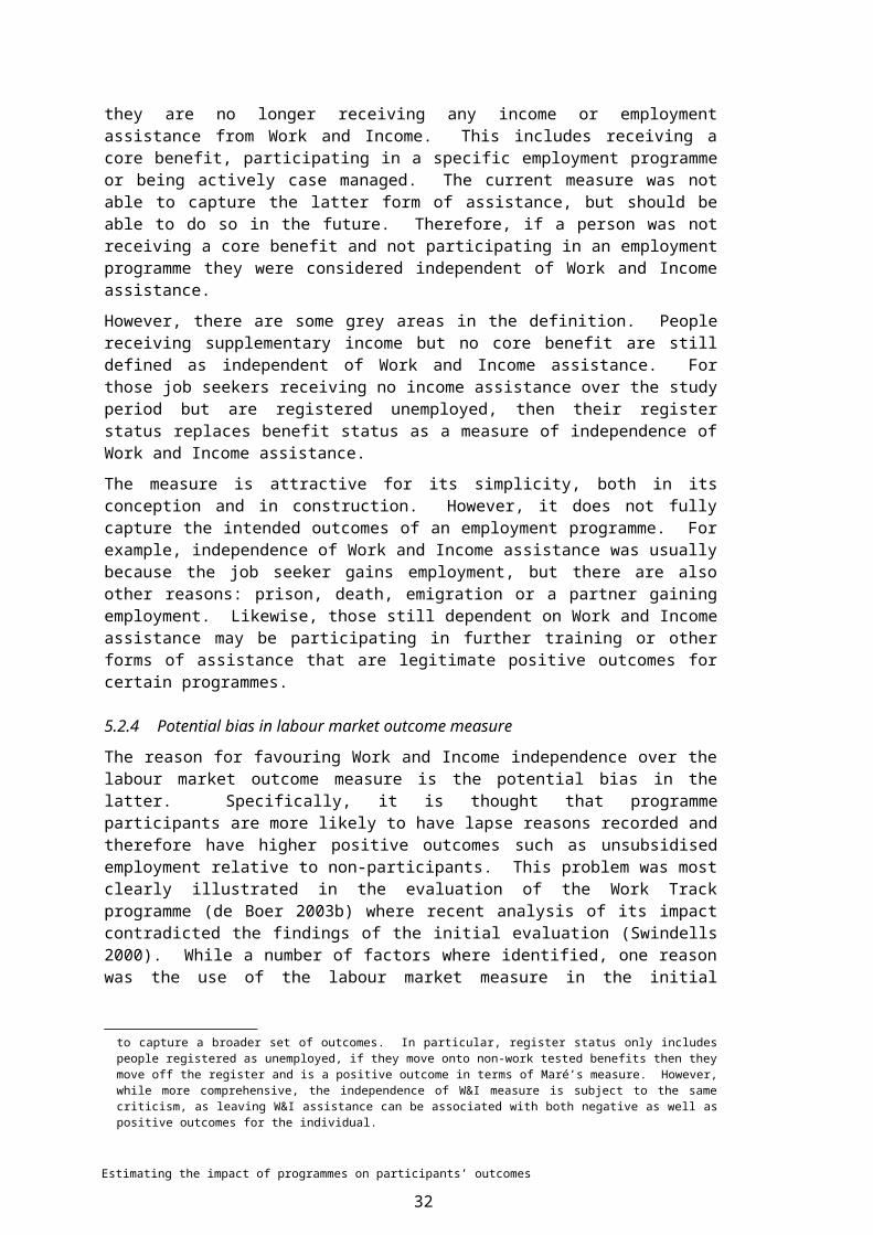
4, True selection biasThe final component of selection bias might be termed “true” selection bias, and refers to the selection of participants on unobserved characteristics that affect outcomes in the absence of the programme (Y0). The argument is that those who are likely to participate in the programme have different outcome probabilities than the eligible population for the programme. How this might come about differs according to the institutional setting, the particular programme and the referral process. For example, who determines selection into the programme: is it voluntary decision by the participant or does the case manager play a significant role? Creaming is often identified as a risk in the selection of people onto programmes, whereby either the case manager favours people with high innate outcome probabilities, or where more motivated people select themselves onto the programme. On the other hand, evidence suggests the converse (Heckman, LaLonde and Smith 1999). In other words, it is those with lower outcome probabilities that have a higher probability of participating in employment programmes.
Lessons learnedIn their review of non-experimental replications of social experiments, Glazerman, Levy and Myers (2002) identify a number of lessons or hypotheses that have emerged from the literature on minimising selection bias in non-experimental designs.
using longitudinal data for several years of pre-programme employment and earnings (Bloom 2000; Ashenfelter and Card 1985; Dehejia and Wahba 1999)
collecting data for the treatment and comparison groups in the same manner, with differences in outcome measurement presenting an important disadvantage (Heckman et al 1997)
controlling properly for observable characteristics, which may remove most (but not all) of selection bias (Heckman et al 1998)
comparing groups of individuals from the same or similar labour markets, which may improve accuracy (Friedlander and Robins 1995; Bell et al 1995; Heckman et al 1998)
using non-experimental estimators for mandatory programmes or those with clearly defined eligibility criteria, which is likely to be more accurate given the lower unobserved selection bias (Bloom et al 2002).
Selection bias in the New Zealand contextWhat implications does this have from selection bias with respect to New Zealand employment programmes? In terms of the first two sources of bias, New Zealand is in a comparatively strong position with evaluators having access to information on all eligible non-participants. This allows non-participant samples to be drawn from the same population and labour markets. Likewise, as Section 4 shows, there is a relatively rich set of information on the characteristics of job seekers, including information on previous benefit receipt. However, a clear omission is information on the previous earnings of job seekers before they become unemployed. Concern is therefore focused on the issue of unobserved selection bias.
6.3 Some possible estimatorsThere exist a number of alternatives to experimental designs. So far, only propensity matching has been the measure used to any great extent in New Zealand. However, the message from the literature is that there is no one single estimation technique that
Estimating the impact of programmes on participants’ outcomes
32

can be applied to all evaluation contexts. An important next stage of the EES is to develop capacity in the application of alternative estimation techniques.
The various estimators discussed in the following section address the issue of selection bias in different ways. The most obvious classification is between experimental designs that actively intervene in the operation of the programme11 and those designs that use ex post facto information to estimate the impact of programmes. However, this distinction is somewhat artificial and the following attempts to place experimental approach within the broader framework of controlling for selection bias.
6.3.1 Key assumptions
All microeconomic or partial-equilibrium estimators make a number of key assumptions, over and above those specific to each of the estimators. It is important to be aware of the role they play in the subsequent interpretation of the final estimators.
All estimators assume that the decision to participate in programmes is determined at the level of the individual and does not depend on the decisions of others (eg peer effects). For example, programme participants encouraging others to join the programme. The significance of the violation of this assumption is whether the peer correlation is related to outcomes, in the sense that more motivated job seekers will respond to this information more so than less motivated job seekers (Bryson, Dorestt, and Purdon 2002). In this example, any estimator that does no account for this will be upwardly biased.
The second assumption is the Stable Unit of Assessment Assumption (STUVA), which states that the impact of the programme on anyone individual does not depend on who else is participating in the programme. This is linked to the issue of accounting for the impact that programmes have on non-participants. For example, if a programme increases the outcomes of participants whilst decreasing the outcomes of non-participants, this would result in an upward bias in the impact estimate.
For simplicity, the following discussion assumes that programme impact is homogeneous relative to participants’ characteristics (X). This “common effect” assumes that the unobservable error term is the same in both treated and untreated states (U0it = U1it = Uit) and that 1(Xit) - 0(Xit) is constant with respect to Xit, where i denotes each individual and t the time period.
6.3.2 Simple estimators
The following estimators are easy to implement and interpret. The disadvantaged is that they require strong assumptions to be valid estimates of programme impact. This does not mean that they cannot be used, but if they are, there needs to be good reason to believe the assumptions are valid.
Pre-post or cross-sectional estimatorThis estimator uses pre-programme outcomes information to impute the counterfactual of post-programme outcomes.
TT = E(, D=1) = E(Y1t, D=1) - E(Y0t, D=1)
Yit – Yit = (Xit) - (Xit) + * + Uit - Uit (3)
where * = is the estimated impact of the programme.
t = observations occurring in the periods after participation start.11 Although it is possible that evaluations can use natural experiments to estimates of programme impact.
Estimating the impact of programmes on participants’ outcomes
33

t’ = observations prior to programme participation.
U = unobserved error term.
If it is assumed that E(Uit - Uit) = 0 and E((Uit - Uit) ((Xit) - (Xit) ) = 0 then equation (3) reduces to Yit – Yit = *. That is, the programme impact on participants’ outcomes is the difference in outcomes before and after the programme. E(U it - Uit) = 0 is the assumption that the outcomes of the participants before and after the programme would be the same if they had not participated ( E(Y0t – Y0t| D=1) = 0 ).
Bias with this estimator occurs in the presence of time-specific intercepts (life-cycle employment changes, economic shocks) that occur concurrently with programme participation. Therefore, before and after is most successful where there are only fixed effects (Uit = ƒi + υit, where ƒi depends on i but does not vary over time and υ it is a random error term). This generally not considered to the case for most employment programmes, where participation is based on time variant factors (eg unemployment). Examples where this technique could be applied is where there is reason to believe that there is no or little effect on the outcome without the intervention, an obvious area is the use of pre- and post-tests to estimate the effect of a training programme on specific skills or knowledge.
Naïve comparison estimatorAnother simple estimation of programme impact is to compare the outcomes of participants to a random group of non-participants.
TT = E(, D=1) = E(Y1, D=1) - E(Y0, D=0). (4)
The assumption is that participants are sufficiently similar to the “average job seeker” in the probability of achieving an outcome to enable any mean difference in outcomes to be attributed to programme impact. This is a very strong assumption, as it ignores any selection bias (see Section 6.2) and for this reason is referred to as the naïve estimator.
6.3.3 Conditioning on observable characteristics
More sophisticated estimates of impact can be divided into two groups, the first are those that control for selection bias based on observed characteristics, while the other uses techniques that explicitly control for unobservable characteristics. The methods developed so far fall into the former category, with no successful implementation of methods employing the latter approach.
Conditional independence assumption (CIA)All cross-sectional estimators; eg naïve, regression on outcomes and matching, rest on the assumption that conditioning on observable characteristics ensures the outcomes of participants and non-participants are identical in the absence of the programme. If the CIA holds, then it can be inferred that any difference in outcomes between participants and non-participants can be attributed to the effect of the programme. Violation of the CIA occurs where there is missing information on characteristics of job-seekers associated with outcomes in the case of outcome regression estimators or information on outcomes and participation in matching estimators. In either case, there will be uncontrolled for differences between participants and non-participants in addition to the effect of the programme, leading to biased estimates.
At present, it is not possible to know whether CIA has been violated, although a number of specification tests do exist. It is more than likely that the CIA is violated in
Estimating the impact of programmes on participants’ outcomes
34

most estimators. The issue is to what extent the violation occurs and therefore what level of bias is likely to exist. For example, there is evidence that the controlling for bias due to observable characteristics is more important than controlling for bias due to unobservable characteristics (Heckman, LaLonde and Smith 1999 and see also Section 6.2 on selection bias). Therefore, while there may be evidence that the CIA is unlikely to hold, there is still merit in controlling for observable bias and employing other techniques to address potential unobserved bias (Bryson, Dorestt and Purdon 2002).
Regression estimatorsThis technique is an advance on the naïve estimator is to condition post programme outcomes on some set of pre-programme characteristics. Formally,
TT = E(|X, D=1) = E(Y1|X, D=1) - E(Y0|X, D=0). (5)
Yit = x(Xit) + y(Yit) + Di* + Uit (6)
where Xit’ and Yit’ are individual characteristics and outcomes covariates observed in the pre-programme period. Bias emerges in the model when E(D i Uit) 0 or if E(Uit
x(Xit’)) 0 or if E(Uit y(Yit)) 0; that is, where any of the terms of the equation are correlated with the error term.
MatchingA less parametric way to control for observed characteristics is to construct a group of non-participants matched in their observed characteristics to the participant group. Formally, there exists a set of conditioning variables (Z) for which non-participant outcomes Y0 is independent of participation status D, conditional on Z (Rosenbaum and Rubin 1983).
Y0 D | Z (7)
In addition, to estimate the treatment on the treated (TT) it is necessary that a match be found for all participants.
Pr(D=1 |Z) < 1 (8)
Based on these two assumptions, the estimate of TT can be written as:
= E(Y1 – Y0 |D=1)
= E(Y1| D=1) – Ez|D=1{EY(Y| D=1, Z)}
= E(Y1| D=1) – Ez|D=1{EY(Y| D=0, Z)}
where the second term can be estimated from the mean outcomes of the matched (on Z) non-participant group (Smith and Todd 2000).
One significant issue in matching on observable characteristics is that increases in the number of characteristics used to match participants and non-participants rapidly decrease the probability that any given participant will have a corresponding matched non-participant. Rosenbaum and Rubin (1983) proved that it is possible to overcome this problem by matching on a scalar of the probability of a given person participating in the programme (hence the term propensity score). Formally the propensity score is derived by:
Di = m
itimmj
ijj UYZ (9)
where
Di = participant (D = 1) or non-participant (D = 0) for each individual
Estimating the impact of programmes on participants’ outcomes
35

Zj = individual i pre-programme observable characteristics
Yit = outcomes in pre-programme period
Ui = unobserved random variation.
Because the dependent variable is binary, the propensity score (Pr(D=1| Z) ) is estimated using a logit model.
Matching versus regression techniquesThere are strong arguments for favouring matching over regression on outcomes. Bryson, Dorestt and Purdon (2002) argue for the unambiguous preference of matching over regression for two reasons. The first is that matching estimators are explicit over the problem of common support, while regression techniques rely on functional form to impute values where common support is weak. The second and related point is that matching techniques do not require functional form assumptions in the outcome equation; this is advantageous, as functional form restrictions are not justified by economic theory or the data used (Smith and Todd 2000). However, propensity matching cannot be considered to be purely non-parametric, as it still uses functional form in deriving the propensity score.
In addition some authors have used combination of matching and regression models see for example (Maré 2000; de Boer 2002). The argument has been that the regression model would further control for differences between participants and matched non-participants. However, in practice there appears to be little gain in combining the two approaches. Most studies have found that the addition of regression controls to a matched sample either produced, at best, very similar estimates as matching alone (Maré 2000; de Boer 2002). Glazerman, Levy and Myers (2002) conclude the reduction in selection bias of combining regression and matching is not significant, although some gains are possible.
6.3.4 Conditioning on unobservable characteristics
The third set of designs focuses on controlling for unobserved characteristics between participants and non-participants. These methods include instrumental variables, econometric selection models (eg Heckman’s two-step procedure) and random control treatment experiments. The principle all these methods share is the identification of a variable that is related to programme participation but is unrelated to participants’ outcomes. Therefore, like the CIA, the assumption is that conditioning on this variable; all observable and unobserved characteristics are randomly distributed between participants and non-participants.
Instrumental variable (IV) estimatorThe IV method is the simplest of this type of design. Once a suitable instrumental variable is identified, it is possible to determine the impact of the programme through the difference in outcome probability between people possessing different values of the instrumental variable. Formally;
)Z|1Pr(D - ) Z| 1Pr(D)|()|(
TT21
21
ZYEZYE
(10)
where TT = impact on the treated
Y = outcomes
Z = instrumental variable with two possible states (Z1, Z2).
Estimating the impact of programmes on participants’ outcomes
36
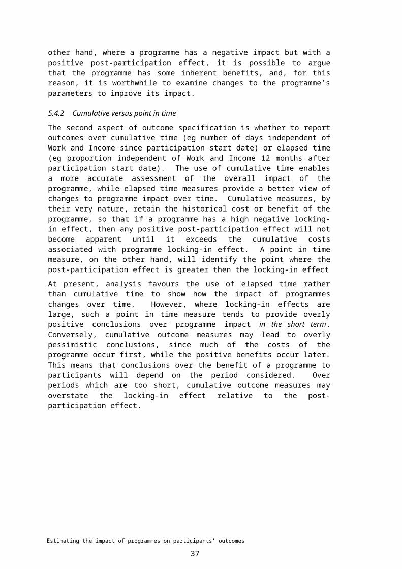
D = participation in programmes (D=1, participant)
While equation 1 estimates the impact on the treated, this may not always be the case, as it depends on the nature of the instrumental variable used. The estimate will reflect the TT only if the instrumental variable is uncorrelated to the gains from the programme; otherwise the parameter estimated is a LATE (Bryson, Dorestt and Purdon 2002). For example, if participants know beforehand the gain from a programme and the IV is distance from the programme, then those further away who do participate would be those who gain more from the programme to compensate for the higher cost of getting to the programme.
The obvious challenge is to be able to identify a suitable IV, and convince people that it is truly uncorrelated to outcomes. In addition, it is also necessary to be sure which parameter is being estimated – LATE or TT. This is especially important if heterogeneous effects are thought to exist and that participation decision are partially or completely based on accurate determination of person-specific impact. In such instances, IV estimators are more likely to estimate some form of LATE rather than the TT. This means that estimates based on instruments unrelated to policy may be of little interest.
Random control treatment designsRandom control treatment designs are one form of IV estimator that involve the direct creation of the IV through the random assignment of potential participants to participant and control groups. This guarantees membership to either group unrelated to outcomes and highly correlated to participation in the programme. Furthermore, and as discussed in Section 3.1.2 it is still possible to provide a valid estimate of TT in the presence of participant drop-out and participation by the control group, as long as there remains a differential in the relative probabilities of participation between the treatment and control group.
While experimental designs are often held up as the “gold standard” for estimating the effect of the treatment on the treated, and there are strong theoretical arguments to say that any estimates are robust and unbiased, there is currently no empirical evidence to confirm this. Specifically, no study has so far established the non-sampling error of experimental designs in the evaluation of employment and training programmes, while a considerable literature exists for non-experimental approaches. Most analysis of the relative effectiveness of alternative estimators assumes zero non-sampling error for experimental impact estimates (see, for example, LaLonde 1986; Bloom, Michalopoulos, Hill, and Lei 2002; Glazerman, Levy and Myers 2002).
Differences in differences estimatorAn extension of the pre-post design is the inclusion of a group of non-participants to act as a baseline to control for time invariant unobservable factors. This may include things such as life-cycle changes, economic shocks and so on. The estimator is essentially the observed difference in outcomes of the participants pre and post programme participation, minus the outcomes of non-participants over the same period (hence the term, difference in difference). Formally;
TT = E(|X, D=1) = E(Y1t|X, D=1) - E(Y0t|X, D=1) – [E(Y0t|X, D=0) - E(Y0t|X, D=0)] (11)
Yit – Yit = * + (Xit) - (Xit) + Uit - Uit . (12)
Like the before and after estimator, the fixed effects estimator works on the assumption that E(Y0t – Y0t | D = 1) = E(Y0t – Y0t | D = 0), in other words, the unobserved change in outcomes of participants in the absence of the programme would be the same as for the observed change among non-participants over the
Estimating the impact of programmes on participants’ outcomes
37
same period. Therefore, while the fixed effects estimator overcomes one of the limitation of the before and after estimator in allowing time-specific variants common to all groups, it is still vulnerable to those time-specific variants that differ between groups.
The problem with this approach with respect to employment and training programmes is that participation is often associated with transitory states (unemployment or “Ashenfelter’s dip” with respect to earnings data) and therefore is inconsistent with pre and post as well as difference in difference estimators as the time-specific variation differs between groups. The presence of such transitory factors leads to bias as well as inconsistencies with estimates depending on the particular pre and post periods used (Heckman and Smith 1999).
6.3.5 Importance of variable selection
Most of the estimation techniques discussed so far make certain requirements of the types of variables that should be included in the estimation for the assumptions of the estimate to hold true, this is particularly the case for those estimates that rely on CIA. Understanding the information requirements of assumptions assists in the assessment of whether the alternative estimates techniques are valid in given evaluation contexts.
Figure 8 groups variables into three sets. The first set is those that influence labour market outcomes or earnings (B, C), while the second is those that influence participation in the programme (C, D). The last set (A) includes those variables that affect neither programme participation nor outcomes, and should be excluded from any analysis of programme impact. The usefulness of this diagram is the ability to categorise different estimation techniques according to the information that they use.
Outcomes or Participation (B, C): before and after, differences in differences, regression.
Participation only (D): instrumental variables and random control treatment experiments.
Participation and Outcomes (C): matching.
Figure 8: Representation of the variables significant in the estimation of programme impact
A
B C D
Outcomes Participation
Estimating the impact of programmes on participants’ outcomes
38

7 Propensity matchingMost effort to date has gone into developing a robust propensity matching method. The decision to start with this estimator was based on the relative simplicity of the concept, while technically complex, the basic idea of propensity matching is easy to convey and understand within a policy and operational environment. In addition, propensity matching can be used in combination with a number of the other estimation techniques discussed above, and therefore provides a useful starting point for any analysis of programme impact.
The extent to which matching provides true estimates of programme impact remains untested in New Zealand. However, studies that have compared alternative non-experimental designs using an experimental benchmark indicate that its performance is good compared to alternatives (Heckman, LaLonde and Smith 1999; Bloom, Michalopoulos, Hill and Lei 2002). However, this goes with the proviso that matching is based on a relatively rich dataset (Bryson, Dorsett and Purdon 2002; Sainesi 2001), a finding confirmed in the New Zealand context (de Boer 2003b). The information available on MSD administrative databases appears to fit this criterion, with one exception, which is information on people’s earnings (refer to Section above).
7.1 Estimating propensity scores by sub-periodA common issue when evaluating employment programmes is the constant change in operational parameters. The concern this raises is that these changes in eligibility or programme parameters will have a significant influence on which job seekers participate in programmes. For example, Training Opportunities was divided into two programmes (Youth Training and Training Opportunities) in 1998, which resulted in a significant shift in the age distribution of Training Opportunities participants before and after this date (see Table 1). In addition, non-programme factors may also influence selection onto programmes. The merger of New Zealand Employment Service and Income Support into the Ministry of Social Development in October 1998 is one example.
Table 1: Age distribution of Training Opportunities participants by year of participation start
Training Opportunities Programmes
Training Opportunities only
Age group 1996 1997 1998 1999 2000 2001
15-17 yr 21.7% 20.3% 9.1% 6.2% 2.6% 0.9%
18-19 yr 16.0% 20.7% 19.8% 19.7% 20.4% 18.2%
20-24 yr 18.7% 18.6% 22.2% 22.6% 22.2% 22.6%
25-29 yr 11.9% 10.7% 13.4% 13.4% 13.6% 13.7%
30-39 yr 17.8% 16.8% 20.1% 21.1% 22.9% 24.1%
40-49 yr 10.8% 10.0% 11.5% 12.8% 13.7% 15.3%
50-54 yr 2.2% 2.0% 2.8% 3.2% 3.2% 3.8%
55-59 yr 0.5% 0.6% 0.7% 0.7% 1.1% 1.0%
60+ yr 0.1% 0.1% 0.1% 0.1% 0.2% 0.3%
Error 0.4% 0.2% 0.2% 0.1% 0.1% 0.0%
Estimating the impact of programmes on participants’ outcomes
39

To address this issue, the propensity to participate in a given programme is modelled for short periods of time (usually one year) to adjust for any underlying changes in programme participation propensity. Where there are few programme participants, then length of the sub-period for each propensity model increased to ensure sufficient participants to maintain statistical power.
7.1.1 Defining the non-participant population
As discussed in Section 3.1, definition of non-participants is not a trivial problem. One issue is the status of previous programme participants. Is it the case that all participants in the programme should be excluded from the non-participant population? If so, how far back should this exclusion extend, especially if the information on programme participation may be unavailable? The approach taken here is to only exclude from the non-participant population the participants who participated in the programme within the specific sub-period being evaluated. An additional issue is the participation by non-participants in similar programmes. In this case, all non-participants who either started or completed this type of programme within one month of their selection date were also excluded.
7.1.2 The problem of common support
In the general form of matching, it is required that for conditioning variables (Z) the probability of being a participant given Z is between, but not equal to, 0 or 1 (0 < Pr(D=1|Z) < 1). However, this restriction can be relaxed when the parameter of interest is the impact of the programme on the treated (TT), in this case the probability of participating has to be less than 1, but can be zero (Pr(D=1 |Z) < 1). In other words, it is important to have a corresponding non-participant for each participant for a given set characteristics, but it is not necessary to have a participant for each non-participant. In the example below, there are no participants that have register durations over 208 weeks, but common support is not compromised if the parameter estimated is the impact on the treated. However, if the parameter in question is the average treatment effect (ATE), then common support is an issue because it is not possible to know the impact of the programme on participants with register durations greater than 208 weeks.
Register duration
Participants Non-participants
0-13 weeks 438 8934
14-25 weeks
230 3647
26-51 weeks
57 2391
52-103 weeks
28 939
104-207 weeks
5 546
208+ weeks 0 983
However, this distribution of participants and non-participants by register duration is problematic in the specification of the logistic model, as it is not possible to the estimate the effect of register duration exceeding 207 weeks.
Estimating the impact of programmes on participants’ outcomes
40

The response to this problem is to exclude those variable classes that contain fewer than two participants.12 In other words, in the above example, all the non-participants with register durations of 208+ weeks would be excluded from the analysis.13 This would mean that for every Z variable there would be both non-participant and participant observations. This reduces the bias that arises from comparing unlike people, or people in different contexts (see Section 6.2).
This raises a further point, in that the purpose of propensity matching is not to specify a model that predicts who will be a programme participant based on a random sample of the eligible population. Rather, it is an alternative technique for modelling the marginal distributions of participants and non-participants along a given number of conditioning variables (Z). In other words, it is a more efficient way in which to identify for each participant and non-participant who share similar sets of observable characteristics.
The reduction in the comparison group to only those who have characteristics common with the participant population increases the risk of common support failing in the other direction; that is for a given participant there are no non-participants with the same characteristic. This risk is most acute if there are high correlations between specific characteristics. To use the example above, the elimination of non-participants with high current unemployment durations would affect the distribution of non-participants by total time spent on income support in the past five years. The contrived result of the elimination of those non-participants unemployed for more than 208+ weeks is that there are now no non-participants who spent more than 90% of the previous five years receiving income support, whilst six participants have done so.
Proportion of time spent on income
support in previous 5 years
Participants Non-participants
0-9% 23 234
10-19% 244 265
20-29% 55 346
30-39% 35 1783
40-49% 789 356
50-59% 123 235
60-69% 23 176
70-79% 45 93
80-89% 12 30
90-100% 6 0
This represents a violation of the common support assumption, as those who have spent more than 90% of their time on income support have an estimated probability of 1 of being a participant ( Pr(D=1|Z) = 1). This problem is most acute for programmes that have specific target groups, and who are not well represented within the general population of non-participants. In the New Zealand context, this often arises in targeting of programmes to specific ethnic groups (most often Maori or Pacific people). For example, a programme targeted at Pacific people, the inclusion of
12 This does mean that some participants have to be excluded from the analysis; however, the numbers involved are relatively small compared to the total number of participants in the models.
13 Use of a continuous variable specification would overcome the problem of a negative Hessian matrix in calculating the maximum likelihood for the logistic model. However, the common support problem is still relevant, as it is still necessary to impute values where Pr(D=1|Z) = 1 or 0.
Estimating the impact of programmes on participants’ outcomes
41

ethnicity as a conditioning variable would result in the exclusion of up to 92% of any general sample of job seekers (ie Pacific people make up about 8% of beneficiaries).
There are four potential solutions to this problem. The first and least desirable is to eliminate those participants with characteristics for whom there are no corresponding non-participants. The two problems this poses are, first, this reduces number of participants, and second, it changes the parameter being estimated. In this case, the impact estimated will no longer be the treatment on the treated, but will be a subset of this group. The second solution, only slightly better than the first, is to remove the conditioning variable from the model (for example, omitting an ethnicity indicator from a programme targeted at a specific ethnic group). This solution could be implemented in practice, as long as it can be shown that the conditioning variable (Z) is unrelated to non-participant outcomes (ie Z is an instrumental variable).14 However, given that most programmes are targeted on the basis of characteristics associated with higher risk of unemployment, this scenario is unlikely.
The last two solutions hold most promise. The first is to increase the size of the initial random sample of non-participants, which should increase the probability that by each characteristic with at least two participants, there will also be more than one non-participant. The main limitation of this solution is its inefficiency when the specific characteristic is uncommon within the non-participant population. This would require drawing a very large sample (most of whom would not be similar to the participants) to be able to have sufficient probability of having sufficient observations in each cell. However, there are limits to the relative size of the non-participant and participant populations, it is preferable not to have a significantly larger non-participant group relative to the participants in the model (the default is not to have more than 10 non-participants for each participant within each logic model).
Therefore, the fourth and preferred option is to introduce specific sub-samples of non-participants. For example, in the case of a programme targeted at Pacific people, include a random sample of Pacific non-participants. This is the most efficient means by which to ensure that the initial non-participant population has the same range of characteristics as the non-participants. The downside of is that the resulting propensity models can no longer be interpreted as showing the relative probability of job seekers participating in the programme (ie the non-participant population is now a non-random sample). However, since this is not the objective of the propensity matching process, this is not a serious problem.
7.1.3 What variables should be included
The purpose of matching and its associated conditional independence assumption (CIA) determines the variables on which participants and non-participants are matched. The CIA requires that once matched, there should be no difference in the distribution of observable characteristics that influence the selection into the programme and the outcome probabilities of participants in the absence of the programme. Variables that affect participation but not outcomes (instrumental variables) can be excluded as well as those that are correlated with outcomes but not participation (see Figure 8,).
Intuitive response to matching is to attempt to use as many observable characteristics as possible, based on the argument that an over parameterised model is better than an under parameterised one. While this is true to some extent, there are risks associated with the inclusion of variables outside the joint condition of influencing outcomes and participation. Variables linked to outcomes but not participation pose little risk given that they will not play a significant role in the propensity model. On the other hand, instrumental variables (affect participation but not outcomes) would, by
14 If this is the case, then it should not be part of the propensity model (see Section 7.1.3).
Estimating the impact of programmes on participants’ outcomes
42

their very nature, lead to problems of common support and matching participants to non-participants. However, neither of these two types of variables would lead to biased estimates. Variables that produce both issues of common support and biased estimates are those that change in response to programme participation rather than influence participation. Examples encountered so far included the receipt of Training Benefit for people moving into training programmes or the dummy for current participation in any programme. Such variables confounded the assumed casual relationship between the dependent (programme participation) and independent variables in the model.
Under parameterisation also poses risks to propensity matching estimator. As stated previously, the CIA is invalid in the presence of significant unobserved (to the evaluator) variables that influence both outcomes and participation. The challenge for evaluators is to be able to assess this risk. For example, if selection process is voluntary with few restrictions, then it is difficult to know what the important determinants of participation might be. At the other extreme, a well-specified set of eligibility criteria reduces uncertainty over who within the population will participate. Nevertheless, even in such cases it is still important to be able to include variables that influence case manager or participant selection onto the programme. For example, while programmes are generally targeted to those considered at risk of long-term unemployment, it is still possible to case manager to “cream” participants or for different types of participants to self-select onto the programme.
The general conclusion from this discussion is that it is most important to have a rich set of variables correlated to labour market outcomes. From this variable set it should be possible to identify those that are vary between participants and non-participants and therefore need to be included in the propensity model. However, in the New Zealand little work has been done to determine which variables that should be considered as part of any propensity model.
7.1.4 Logistic model specification
Specification of the logistic model is based on the balancing test (see Appendix 1). The balancing test determines whether the propensity score achieves its stated aim, that is, conditional on propensity score it is not possible to tell whether a person is a participant or non-participant based on any observable characteristic. Rosenbaum and Rubin (1983) present a theorem that helps determine whether the model includes all relevant Z variables and whether it is necessary to include interaction terms.
Z D | Pr(D=1|Z)
E(D|Z, Pr(D=1|Z) = E(D|Pr(D=1|Z)) (13)
The idea from this theorem is to test whether there are differences in Z between participant (D=1) and non-participant groups (D=0) after conditioning on Pr(D=1|Z).
The balancing test involves the following steps:
1. Fit the propensity model using an parsimonious selection of variables known to influence outcomes and participation.
2. Match non-participants to participants using nearest neighbour matching (see Section 7.3.1,).
3. Split the participants and non-participants into k equally spaced intervals of the propensity score, k being defined initially as five.
4. Within each interval, test for difference in the average propensity score between participants and non-participants.
Estimating the impact of programmes on participants’ outcomes
43

5. If the test fails for a given interval, split the interval and half and re-test until there are no significant differences in any interval.
6. Within each interval, test differences in the mean and distribution of each variable (not just those included in the propensity model) between participants and non-participants.
7. If the means / distributions do differ for a given variable, then select a less parsimonious model specification, either through the addition of variables, higher order terms or interactions.
The inclusion of distributions for a number of variables generally goes beyond what is practiced in the literature (Becker and Ichino 2002; Dehejia and Wahba 2002). However, only testing mean values implies assumptions of normality in the distributions of these variables, an assumption that is unlikely to hold in most instances. In addition, it is also necessary to randomly split the participant and initial non-participant sample into two groups, construct the propensity model on one and, once completed, apply the model to the other sample. This ensures that the model is not “over-fitted” to the data, based on random variation in the observed characteristics of participants and non-participants.
The significance level for differences is set at 0.01. While this is a high level of significance, implying differences would have to be large to fail the balancing test, this is justified on two reasons. The first is that the observations involved tend to be large (>1,000) increasing the likelihood of insubstantial differences having a statistically significant difference. The second reason is that the test is applied to each variable (and its distribution), which means that, if the balancing test is strictly adhered to, it would fail if only one of these differences was significant. There is an increased statistical probability of this occurring as the number of variables increase. For example, taking five variable and five intervals of the propensity score would require 25 mutually independent tests of mean differences (step 6 above). For this balancing test, there is a probability of 0.2015 that one of these tests is significant although the balancing test is true.
In practice it is difficult to get all the variables to balance and therefore in the following examples the aim was to ensure the majority of variables to be balanced for at least 90% of the participant distribution.
7.2 Summary of logistic modelModel fit statistics
Table 2 is a summary of Training Opportunities propensity models for the four quarters of 1996. The model correctly identified 76% of participants as participants; this figure was 72% for non-participants. Allocation into the predicated participant and non-participant groups was based on whether a person’s propensity score was greater or less than the proportion of participants in the original sample. The value “true participants” is the proportion of the participant group correctly identified as being a participant by the model (ie their propensity score is above the cut-off value).
15 20.099.001.0125 241
Estimating the impact of programmes on participants’ outcomes
44

Table 2: Propensity Training Opportunities 1996 Model fit statistics
Model period 01-Jan-96 to 31-Dec-96
Observations 30,856
Participants 4,995
Non-participants 25,861
Convergence criteria Satisfied
2logL Intercept Only 27,325
2logL Model 20,070
Likelihood Chi Square *** 7,255
Likelihood df 181
True Non-participants 72%
True Comparison 76%
Propensity Cut-off 0.16
Lackfit test (8 df) ** 18
*: 0.05<p<=0.1, **: 0.1<p<=0.05, ***: p<=0.01
Propensity cut-off was the proportion of participants within the model. True participants are those participants with a propensity score above the cut-off, whilst true comparison is the proportion of non-participants with a propensity score below the cut-off value.
Lackfit: Homer-Lemeshow (1982) goodness of fit test.
On the other hand, the Lackfit test suggests the goodness of model fit was not high, being significant at p <0.10. However, as emphasised earlier, this is not an issue given that the models with high levels of identification (ie clearly distinguishes participants from non-participants) implies that the sample of non-participants is quite unlike the participants. This would make the construction of a suitable matched comparison group problematic, as it would have to significant weight on only a small proportion of the non-participants who look most like the participants. Instead, the success of the propensity models depends on the balance of observable characteristics between participants and matched non-participants (see Section 7.2.2,).
Variable type 3 effects
Table 3 shows the Type 3 chi-square values of the main effects and interactions of the propensity model.16 Higher order terms are indicated by the “**” so that variable X ** 2 means that this variable has been squared. The full results for the model are given in Appendix 2.
16 Full summaries of the propensity models and associated analysis can be provided on request by the author.
Estimating the impact of programmes on participants’ outcomes
45

Table 3: Propensity Matching Training Opportunities Type 3 effectsModel Period 01-Jan-96 to 31-Mar-96
Age group (8 df) *** 499.0Age of Youngest Child (3 df) *** 3.0
Benefit Type (6 df) *** 414.0CurPar - InfoService (1 df) *** 73.0
CurPar - Wage Subsidy (1 df) *** 41.0CurPar - Work Confidence (1 df) *** 22.0CurPar - Work Experience (1 df) *** 16.0
Current Benefit Duration (wks) (1 df) *** 10.0Current Benefit Duration ** 2 (1 df) *** 6.0Current DWI Duration (wks) (1 df) *** 39.0
Current DWI Duration (wks)*Current Regis (1 df)
*** 0.0
Current DWI Duration ** 2 (1 df) *** 32.0Current DWI Duration ** 3 (1 df) *** 28.0
Current Register Duration (wks) (1 df) *** 23.0Disability - Any (1 df) *** 2.0
DWI region (12 df) *** 126.0Ethnicity (3 df) *** 72.0Gender (1 df) *** 34.0
Highest Qualification (7 df) *** 111.0Intercept ( df)
Ministerial Eligibility (1 df) *** 142.0Period Started (3 df) *** 492.0
PrePar - Any Programme (1 df) *** 0.0PrePar - Training (1 df) *** 3.0
PrePar - Training*Work and Income Outcomes Qtr -1 (6 df)
*** 72.0
PrePar - Training*Work and Income Outcomes Qtr -2 (6 df)
*** 17.0
PrePar - Training*Work and Income Outcomes Qtr -3 (6 df)
*** 26.0
PrePar - Training*Work and Income Outcomes Qtr -5 (6 df)
*** 25.0
PrePar - Work Experience (1 df) *** 1.0prgtrpp2 (1 df) *** 2.0prgtrpp3 (1 df) *** 0.0
Proportion Benefit Contact (1 df) *** 8.0regp2 (1 df) *** 5.0
TLA region (49 df) *** 210.0Work and Income Outcomes Qtr -1 (6 df) *** 945.0Work and Income Outcomes Qtr -2 (6 df) *** 145.0Work and Income Outcomes Qtr -3 (6 df) *** 19.0Work and Income Outcomes Qtr -4 (6 df) *** 40.0Work and Income Outcomes Qtr -5 (6 df) *** 8.0Work and Income Outcomes Qtr -6 (5 df) *** 52.0Work and Income Outcomes Qtr -7 (5 df) *** 17.0Work and Income Outcomes Qtr -8 (5 df) *** 34.0*: 0.05<p<=0.1, **: 0.1<p<=0.05, ***: p<=0.01
Estimating the impact of programmes on participants’ outcomes
46
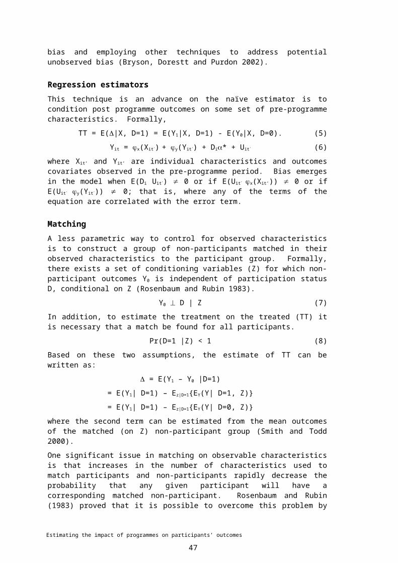
7.2.1 Distribution of participants and non-participants by propensity score
Figure 9 below shows the relative distribution of Training Opportunities participants and non-participants by propensity score. Non-participants are concentrated at the lower propensity scores while participants have a bimodal distribution, with an unusually high concentration in the upper range of the propensity distribution. It should be re-emphasised that the propensity distributions shown here do not reflect the true participation likelihood, as the non-participant group is not a simple random sample of the non-participant population (see Section 7.1.2). Instead, this figure is useful in assessing the levels of common support between the two groups. In this respect, Figure 9 illustrates a typical pattern of propensity scores between participants and non-participants, with non-participants’ scores concentrated in the lower range of propensity values (<0.20), while the participant distribution is skewed towards the higher values.
The issue of common support can be clearly seen, as the proportion of non-participants with propensity scores above 0.5 is considerably less than that of the participants (2.3% versus 33.6%). However, this may not be as serious problem as these numbers suggest, as the non-participant sample is larger than the participant population. In this respect, Figure 10 provides a better guide by showing the ratio of participants to non-participants at each 5/100 of the propensity distribution. What this shows is that as the propensity score increases the number of participants per non-participant increases steadily, with non-non-participants with propensity scores higher than 0.95. Table 4 summarises the participant to non-participant ratios for a number of other programmes included in the analysis. In these instances, there is considerable overlap in the propensity distribution of participants and non-participants, even in the upper range of propensity scores.
Figure 9: Frequency distribution of propensity scores for Training Opportunities (1996) participants and non-participants
0.0%
5.0%
10.0%
15.0%
20.0%
25.0%
30.0%
35.0%
Propensity Score
Fre
quen
cy
Participants 1.8 8.3 10.1 9.5 8.1 7.3 6.8 5.9 4.2 3.9 3.1 2.4 2.3 2.1 2.4 3.1 3.3 4.3 3.9 2.2 5.1
Comparison 19.8 31.6 16.9 10.3 6.7 4.7 3.0 2.2 1.5 1.1 0.7 0.5 0.3 0.2 0.1 0.1 0.1 0.1 0.1 0.0 0.0
0 0.1 0.2 0.3 0.4 0.5 0.6 0.7 0.8 0.9 1
Base: Participants - 4,992, Non-participants - 25,858
Source: Information Analysis Platform, MSD administrative data, 2002
Estimating the impact of programmes on participants’ outcomes
47

What is also apparent from Table 4 is that for a number of programmes, there appear to some issues of common support, whereby at the very high propensity scores (>0.90) there are participants without corresponding non-participants. In this instance, it was not possible to calculate the participant to non-participant ratio. The following section on constructing a comparison group from the non-participant population will examine the effect this has on the observed bias.
Table 4: Ratio of participants to non-participants by propensity score for selected programmes
Propensity score
0.00-0.04 0.25-0.29 0.50-0.54 0.75-0.79 0.95-1Training Opportunities
(1996)0.02 0.30 0.82 4.97 12.22
Community Task Force (1996)
0.01 0.35 0.84 2.75 7.30
Enterprise Allowance (1996)
0.01 0.38 0.87 1.67
Job Plus (1996) 0.01 0.35 1.03 4.11 61.00
Work Confidence (1998) 0.01 0.31 1.08 2.41 ~
Job Search (1996) 0.02 0.36 0.98 2.04 3.15
~: no non-participants in the propensity interval.
7.2.2 Balancing test
On completion of the logistic model, it is important to know whether the propensity score achieves its stated aim. That is, using propensity scores only, it is not possible to tell whether a person is a participant or non-participant based on any observable
Figure 10: Ratio of Training Opportunities (1996) participants to non-participants by propensity score
0.00
2.00
4.00
6.00
8.00
10.00
12.00
14.00
16.00
Propensity Score
Rat
io o
f par
ticip
ants
to n
on-p
artic
ipan
ts
Ratio 0.02 0.05 0.12 0.18 0.23 0.30 0.43 0.51 0.54 0.70 0.82 1.02 1.41 1.93 3.64 4.97 7.22 13.5 14.8 12.2 0.00
0 0.1 0.2 0.3 0.4 0.5 0.6 0.7 0.8 0.9 1
Base: Participants - 4,992, Non-participants - 25,858
Source: Information Analysis Platform, MSD administrative data, 2002
Estimating the impact of programmes on participants’ outcomes
48

characteristic. The results of the balancing test for Training Opportunities (1996) are given in Table 5, which shows the means and distributions of participants, matched non-participants and original non-participant sample. The extent to which the propensity model balanced observable characteristics across the propensity scores is shown as the proportion of participants where there was no statistical difference to matched non-participants for each variable. For example, a balancing score of 100% means that the variable balanced across all propensity intervals, while 80% shows that the variable balanced across those intervals where 80% of the participants are located. The inclusion of the original non-participant sample is to help identify where there may be significant differences between the participants and initial non-participant population. Where such differences occur it may be necessary to consider including sub-samples to ensure that there are sufficient non-participants with characteristics similar to the participants.
Table 5: Demographic profile of Training Opportunities participants, weighted comparison group and job seeker average for 1996.
Variable ClassBalance (% of participants)
Observed Bias Participants
Matched Non-participants
Non-participants
Ethnicity European 92% -2.4 % 39.7 % 42.1 % 50.0 %
Maori 96% 1.5 % 43.4 % 42.0 % 37.6 %
Pacific People 96% 0.8 % 10.8 % 9.9 % 7.9 %
Other 96% 0.1 % 6.1 % 6.0 % 4.5 %
Gender Female 96% 1.2 % 39.9 % 38.7 % 37.0 %
Male 96% -1.2 % 60.1 % 61.3 % 63.0 %
Age in years (blank) 91% -1.39 yr 26.08 yr 27.47 yr 26.00 yr
Age group 15-17 yr 92% 10.9 % 21.1 % 10.2 % 10.1 %
18-19 yr 93% -3.0 % 17.1 % 20.2 % 25.5 %
20-24 yr 100% -2.2 % 19.2 % 21.4 % 27.7 %
25-29 yr 96% -1.6 % 11.9 % 13.4 % 9.8 %
30-39 yr 96% -1.4 % 17.5 % 19.0 % 13.8 %
40-49 yr 100% -1.9 % 10.3 % 12.2 % 9.0 %
50-54 yr 100% -0.5 % 2.3 % 2.9 % 2.9 %
55-59 yr 100% -0.1 % 0.6 % 0.6 % 1.1 %
60+ yr 100% -0.1 % 0.0 % 0.1 % 0.2 %
Disability - Any Yes 100% -1.5 % 8.4 % 9.9 % 9.0 %
Refugee Yes 100% 0.0 % 0.0 % 0.0 % 0.0 %
Highest Qualification
None 96% 3.1 % 63.1 % 59.9 % 51.4 %
School Certificate 95% -0.4 % 23.8 % 24.3 % 23.5 %
Secondary above SC 94% -1.6 % 7.4 % 9.0 % 14.5 %
Post School 89% -1.1 % 5.7 % 6.8 % 10.7 %
Ministerial Eligibility
Not Eligible 88% 9.3 % 48.2 % 38.9 % 54.6 %
26+weeks 92% -9.3 % 51.8 % 61.1 % 45.4 %
SGI group SGI 99 96% 0.0 % 100.0 % 100.0 % 100.0 %
SGI score (blank) 96% 0.00 pnts 0.00 pnts 0.00 pnts 0.00 pnts
Partner Yes 100% -2.1 % 15.5 % 17.6 % 14.5 %
Number of ChildrenNone 96% 1.0 % 89.9 % 88.9 % 92.9 %
1 Child 100% -0.3 % 6.0 % 6.3 % 4.4 %
2+ Child 96% -0.7 % 4.0 % 4.8 % 2.7 %
Age of Youngest Child No Child 96% 1.0 % 89.9 % 88.9 % 92.9 %
Estimating the impact of programmes on participants’ outcomes
49

Variable ClassBalance (% of participants)
Observed Bias Participants
Matched Non-participants
Non-participants
0-5 yr 100% -0.8 % 4.9 % 5.7 % 3.8 %
6-13 yr 100% -0.4 % 4.1 % 4.5 % 2.6 %
14+ yr 100% 0.2 % 1.0 % 0.9 % 0.7 %
CurPar - Any Programme 0% 0% 80.6 % 100.0 % 19.4 %
CurPar - InfoService 95% 95% -0.5 % 6.4 % 6.9 %
CurPar - Into Work 100% 100% -0.2 % 0.3 % 0.5 %
CurPar - Job Search 100% 100% -0.2 % 1.7 % 2.0 %
CurPar - Training 0% 0% 100.0 % 100.0 % 0.0 %
CurPar - Wage Subsidy 100% 100% -0.3 % 1.1 % 1.5 %
CurPar - Work Confidence 62% 62% -1.4 % 7.2 % 8.7 %
CurPar - Work Experience 100% 100% -0.4 % 1.0 % 1.4 %
PrePar - Any Programme 89% 69% 9.40 days 56.19 days 46.79 days
PrePar - Job Search 96% 96% 0.00 days 0.12 days 0.11 days
PrePar - Other 96% 96% 0.00 days 0.00 days 0.00 days
PrePar - Training 89% 69% 11.29 days 45.81 days 34.53 days
PrePar - Wage Subsidy 96% 96% -1.39 days 6.64 days 8.03 days
PrePar - Work Confidence 96% 96% -0.01 days 0.33 days 0.34 days
PrePar - Work Experience 96% 96% -0.49 days 3.29 days 3.78 days
Benefit Type Unemployment 92% 1.4 % 90.1 % 88.7 % 88.5 %
Independent Youth 100% -0.6 % 1.5 % 2.2 % 6.1 %
Domestic Purposes 96% 0.0 % 3.5 % 3.6 % 1.6 %
Emergency 100% -0.1 % 2.1 % 2.2 % 2.0 %
Widows 100% 0.0 % 0.0 % 0.0 % 0.0 %
Invalids 100% -0.3 % 0.7 % 1.0 % 0.4 %
Sickness 100% -0.5 % 1.9 % 2.4 % 1.4 %
Current Benefit Duration (wks) 96% 96% -9.05 wks 102.63 wks 111.68 wks
Current Benefit Duration
0-13 wks 92% 6.7 % 25.8 % 19.0 % 33.6 %
14-25 wks 96% -0.6 % 8.4 % 9.0 % 11.2 %
26-51 wks 92% -2.3 % 18.8 % 21.1 % 15.1 %
52-103 wks 99% -1.2 % 17.0 % 18.2 % 15.5 %
104-207 wks 93% -1.5 % 12.8 % 14.3 % 11.2 %
208+ wks 100% -1.1 % 17.3 % 18.4 % 13.4 %
Proportion Benefit Contact 85% 85% -4.71 pnts 48.89 pnts 53.60 pnts
Current DWI Duration (wks) 96% 96% -13.10 wks 138.12 wks 151.23 wks
Current DWI Duration
0-13 wks 86% 5.5 % 17.2 % 11.7 % 23.0 %
14-25 wks 90% 1.1 % 7.2 % 6.1 % 9.3 %
26-51 wks 88% -0.6 % 16.5 % 17.1 % 14.3 %
52-103 wks 100% -1.7 % 16.3 % 18.0 % 16.4 %
104-207 wks 93% -2.0 % 15.7 % 17.7 % 14.7 %
208+ wks 100% -2.2 % 27.2 % 29.3 % 22.4 %
Proportion DWI Contact 85% 85% -4.71 pnts 48.89 pnts 53.60 pnts
Current Register Duration (wks) 96% 96% -12.15 wks 52.00 wks 64.15 wks
Current Register Duration
0-13 wks 51% 10.6 % 38.2 % 27.6 % 37.8 %
14-25 wks 100% -1.3 % 10.0 % 11.3 % 16.9 %
26-51 wks 89% -2.9 % 23.4 % 26.3 % 18.1 %
52-103 wks 96% -3.6 % 14.3 % 17.9 % 13.2 %
Estimating the impact of programmes on participants’ outcomes
50
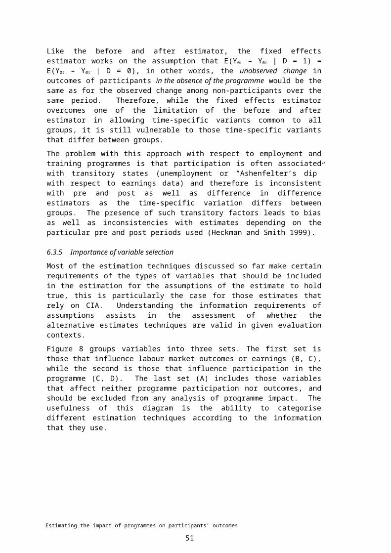
Variable ClassBalance (% of participants)
Observed Bias Participants
Matched Non-participants
Non-participants
104-207 wks 100% -1.0 % 8.3 % 9.4 % 7.5 %
208+ wks 96% -1.8 % 5.8 % 7.6 % 6.5 %
Proportion Work Contact 96% 96% -5.74 pnts 34.22 pnts 39.96 pnts
Work and Income Outcomes Qtr -1
Independent of Work and Income 96% 9.0 % 12.8 % 3.8 % 1.3 %
Dependent on Work and Income 88% -20.9 % 67.4 % 88.3 % 94.8 %
Training 75% 12.5 % 17.6 % 5.0 % 2.2 %
Job Search 100% 0.2 % 0.5 % 0.4 % 0.1 %
Wage Subsidy 100% -0.3 % 0.5 % 0.8 % 0.8 %
Work Confidence 100% -0.2 % 0.8 % 0.9 % 0.4 %
Work Experience 100% -0.3 % 0.5 % 0.8 % 0.4 %
Work and Income Outcomes Qtr -2
Independent of Work and Income 92% 5.3 % 15.9 % 10.6 % 23.2 %
Dependent on Work and Income 85% -15.8 % 60.4 % 76.2 % 67.8 %
Training 78% 11.0 % 20.0 % 9.0 % 5.9 %
Job Search 100% 0.1 % 0.5 % 0.4 % 0.3 %
Wage Subsidy 100% -0.5 % 1.3 % 1.8 % 1.6 %
Work Confidence 100% 0.0 % 0.9 % 0.9 % 0.6 %
Work Experience 100% -0.1 % 1.0 % 1.1 % 0.6 %
Work and Income Outcomes Qtr -3
Independent of Work and Income 82% 5.7 % 22.0 % 16.3 % 29.1 %
Dependent on Work and Income 97% -11.3 % 55.6 % 66.9 % 57.0 %
Training 96% 6.5 % 18.2 % 11.6 % 9.2 %
Job Search 100% -0.2 % 0.4 % 0.6 % 0.4 %
Wage Subsidy 100% -0.6 % 1.8 % 2.4 % 2.4 %
Work Confidence 100% -0.2 % 0.8 % 1.0 % 0.9 %
Work Experience 100% -0.1 % 1.2 % 1.2 % 0.9 %
Work and Income Outcomes Qtr -4
Independent of Work and Income 89% 6.1 % 30.9 % 24.8 % 32.0 %
Dependent on Work and Income 100% -9.1 % 48.9 % 58.0 % 52.7 %
Training 89% 4.0 % 15.6 % 11.5 % 10.0 %
Job Search 100% -0.1 % 0.4 % 0.5 % 0.5 %
Wage Subsidy 100% -0.4 % 2.3 % 2.7 % 2.7 %
Work Confidence 100% -0.2 % 0.7 % 0.9 % 1.0 %
Work Experience 100% -0.3 % 1.4 % 1.7 % 1.1 %
Work and Income Outcomes Qtr -5
Independent of Work and Income 85% 5.9 % 36.5 % 30.6 % 36.4 %
Dependent on Work and Income 100% -6.7 % 46.1 % 52.8 % 49.9 %
Training 85% 1.9 % 13.3 % 11.4 % 8.6 %
Job Search 100% 0.0 % 0.1 % 0.1 % 0.3 %
Wage Subsidy 100% -0.4 % 2.5 % 3.0 % 2.7 %
Work Confidence 100% -0.2 % 0.5 % 0.7 % 0.8 %
Work Experience 100% -0.5 % 0.9 % 1.4 % 1.2 %
Estimating the impact of programmes on participants’ outcomes
51

Variable ClassBalance (% of participants)
Observed Bias Participants
Matched Non-participants
Non-participants
Work and Income Outcomes Qtr -6
Independent of Work and Income 82% 9.0 % 57.4 % 48.4 % 46.8 %
Dependent on Work and Income 100% -9.7 % 26.0 % 35.8 % 41.9 %
Training 85% 1.6 % 12.7 % 11.1 % 7.0 %
Wage Subsidy 100% -0.3 % 2.4 % 2.7 % 2.6 %
Work Confidence 100% -0.2 % 0.3 % 0.5 % 0.6 %
Work Experience 100% -0.4 % 1.2 % 1.5 % 1.2 %
Work and Income Outcomes Qtr -7
Independent of Work and Income 85% 7.2 % 68.4 % 61.2 % 59.4 %
Dependent on Work and Income 100% -7.7 % 16.7 % 24.3 % 30.8 %
Training 85% 0.8 % 11.7 % 10.9 % 6.1 %
Wage Subsidy 100% -0.4 % 2.0 % 2.4 % 2.3 %
Work Confidence 100% -0.1 % 0.5 % 0.5 % 0.4 %
Work Experience 100% 0.2 % 0.8 % 0.6 % 1.0 %
Work and Income Outcomes Qtr -8
Independent of Work and Income 85% 3.7 % 80.1 % 76.4 % 72.5 %
Dependent on Work and Income 100% -2.8 % 6.5 % 9.3 % 18.2 %
Training 85% -0.1 % 10.6 % 10.7 % 6.0 %
Wage Subsidy 100% -0.4 % 1.6 % 2.0 % 2.0 %
Work Confidence 100% -0.2 % 0.4 % 0.6 % 0.3 %
Work Experience 100% -0.2 % 0.8 % 1.0 % 0.9 %
Period Started 1996/1 30% 10.8 % 45.0 % 34.2 % 20.7 %
1996/2 82% -3.3 % 18.7 % 22.0 % 22.9 %
1996/3 75% -4.4 % 27.4 % 31.7 % 27.2 %
1996/4 90% -3.1 % 9.0 % 12.1 % 29.2 %
DWI region Auckland Central 89% -0.6 % 5.8 % 6.4 % 7.0 %
Auckland North 97% -0.7 % 7.1 % 7.8 % 6.4 %
Auckland South 96% -0.9 % 9.0 % 9.9 % 8.7 %
Bay of Plenty 96% 0.1 % 10.2 % 10.1 % 10.1 %
Canterbury 100% -1.1 % 7.2 % 8.3 % 10.2 %
Central 96% -0.9 % 6.6 % 7.5 % 6.9 %
East Coast 100% -0.5 % 7.7 % 8.3 % 7.9 %
Nelson 96% 0.0 % 6.1 % 6.1 % 4.5 %
Northland 100% -0.5 % 6.4 % 6.9 % 6.0 %
Southern 100% 0.0 % 8.6 % 8.6 % 9.2 %
Taranaki 100% -0.3 % 6.9 % 7.2 % 7.4 %
Waikato 100% 0.3 % 6.3 % 6.0 % 7.3 %
Wellington 92% 5.1 % 12.1 % 7.0 % 8.4 %
Source: Information Analysis Platform, MSD 2003.
7.3 Propensity matchingOnce the propensity scores are determined, the next stage of the analysis involves matching non-participants to participants. The literature identifies a number of
Estimating the impact of programmes on participants’ outcomes
52

different approaches (see for example Smith and Todd 2000; Bloom, Michalopoulos, Hill, Lei 2002). However, only two of these methods have been developed in this analysis: stratification/interval and nearest neighbour.
7.3.1 Nearest neighbour matching
Nearest neighbour matching is the most intuitively appealing of all the matching techniques, as it attempts to match each participant with one non-participant whose propensity score is most similar to the participant’s. The impact of the programme for that participant will be the difference in their outcome and that of their matched non-participant. The overall impact of the participants is the mean of these differences.
The only complication arises in this method is whether non-participants can only be used once (non-replacement) or can be matched with more than one participant (replacement). This is an issue of trading observable bias against standard error. Non-replacement techniques ensure that the non-participants and participants are equal in number, thereby minimising the standard error of the estimate, but increasing the bias (where a given non-participant is the best match for several non-participants, they can only be used once). Replacement has the opposite effect, minimising bias by allowing the smallest difference in propensity score to exist between each participant/non-participant pair, but at the cost of having fewer unique non-participants in the final sample.
The approach favoured in this analysis is to select with replacement. This is because the available non-participant population is large compared to the participants, unlike other contexts whether the non-participant sample is fixed due to the high cost of gathering additional observations on non-participants. This means that if the level of replacement is considered to be too high, it is possible to add further sub-samples to increase the similarity in observable characteristics between participants and non-participants. In addition, non-replacement is computationally resource intensive when the number observations is large (>10,000) and is not well suited for regular impact monitoring.
7.3.2 Interval or stratification matching
Interval matching works on the principle of grouping participants and non-participants with similar propensity scores together. Then it is a matter of subtracting the mean outcomes of the participants from non-participants within the same interval of the propensity distribution and aggregating these differences weighted by the distribution of participants in each propensity interval.
The first question is what propensity interval to use. Intuitively, it would be best to have relatively small intervals so that participants and non-participants with similar propensity scores are compared. The trade off is that there is an increased probability of a given propensity interval lacking either participants or non-participants. In other words, the common support condition fails to hold. The technique used in this analysis was to select the interval based on the smallest propensity interval that ensured that every interval had at least one non-participant for each participant. In practice, this involved an algorithm testing this condition with gradually increasing propensity intervals, starting with 0.01 and increasing by iterations of 0.001.
Once the intervals where determined, each non-participant was assigned a weight equivalent to the ratio of participants and non-participants within the interval. For example, if the propensity interval 0.90-0.92 contained 100 participants and 10 non-participants, then each non-participant was given a weight of 10 (100/10). All participants had a weight of one.
Estimating the impact of programmes on participants’ outcomes
53

7.3.3 Does the matching approach matter?
The question of having more than one matching technique is whether different approaches produce different levels of observed bias and ultimately different impact estimates. To answer the first part, the level and distribution of observed bias does differ between the two approaches. Figure 11 illustrates the difference in propensity score between participants and non-participants by propensity score, when using interval matching. The general pattern is that within interval differences are quite small; in the case of Training Opportunities (1996), the mean absolute difference did not exceed 0.006.
Differences in propensity scores between participants and non-participants using nearest neighbour matching (with replacement) are also small (Figure 12,). Where there is strong common support, there is no significant difference in the propensity scores of participants and matched non-participants. However, at higher propensity scores (>0.6) the fall in common support increases the observed bias between participants and matched non-participants. In the case of Training Opportunities (1996), the mean absolute observed bias in propensity scores reaches 0.003.
To what extent this observable bias is an issue is also related to the number of participants affected. For example, if the common support failed for a small proportion of the participants, the observable bias would be large but only affect a small number of observations. To examine this further, Table 6 contrasts the observed bias for nearest neighbour matching with the proportion of participants affected. In general, where observed bias large, the number of participants affected is proportionally very small.
Estimating the impact of programmes on participants’ outcomes
54

Figure 11: Mean and absolute mean difference in propensity scores using interval matching for Training Opportunities (1996)
-0.0005
0
0.0005
0.001
0.0015
0.002
0.0025
0.003
0.0035
0 0.1 0.2 0.3 0.4 0.5 0.6 0.7 0.8 0.9 0
Propensity Score
Diff
eren
ce in
pro
pens
ity s
core
Mean difference Mean absolute difference
Base: Participants - 4,739, Unique Non-participants - 25,855
Source: Information Analysis Platform, MSD administrative data, 2002
Table 6: Distribution of absolute means observed bias and participations by propensity score for selected programmes using nearest neighbour matching with replacement
Propensity scoreProgramme (year) 0-0.05 0.25-0.29 0.50-0.54 0.75-0.79 0.95-1Training Opportunities (1996)
Absolute mean bias
0.0000 0.0000 0.0001 0.0005 0.0020
Participants (%)
1.9% 7.7% 3.3% 3.2% 2.3%
Enterprise Allowance (1996)
Absolute mean bias
0.0000 0.0001 0.0002 0.0021 0.0000
Participants (%)
3.7% 8.4% 4.7% 1.0% 0.0%
Work Confidence (1998)
Absolute mean bias
0.0000 0.0001 0.0005 0.0011 0.0000
Participants (%)
4.7% 7.2% 6.0% 3.8% 0.0%
Community TaskForce (1996)
Absolute mean bias
0.0000 0.0000 0.0002 0.0005 0.0019
Participants (%)
0.1% 8.7% 2.7% 3.4% 1.5%
Job Plus (1996) Absolute mean bias
0.0000 0.0000 0.0002 0.0011 0.0111
Participants (%)
0.3% 13.2% 2.7% 1.6% 1.0%
Job Search (1996) Absolute mean bias
0.0000 0.0000 0.0001 0.0004 0.0014
Participants (%)
0.2% 9.4% 6.2% 2.0% 1.2%
Estimating the impact of programmes on participants’ outcomes
55

Effect of matching technique on impact estimates
Table 7: Estimated impact of Training Opportunities (1996) on proportion of time participants are independent of Work and Income assistance over various lapse periods
Lapse Period 0 to 3 mths
0 to 6 mths
0 to 12 mths
0 to 24 mths
0 to 36 mths
Interval Matching
Participation 5.7% 10.9% 17.5% 24.3% 27.9%
Non-participation
20.9% 25.2% 30.3% 35.0% 38.1%
Impact Ratio 0.27 0.43 0.58 0.69 0.73
Base: Participants
4,992 4,992 4,992 4,992 4,992
Nearest Neighbour
matching with replacement
Participation 5.7% 10.9% 17.5% 24.3% 27.9%
Non-participation
20.2% 24.9% 30.2% 34.7% 37.5%
Impact Ratio 0.28 0.44 0.58 0.70 0.74
Base: Participants
4,992 4,992 4,992 4,992 4,992
Source: Information Analysis Platform, MSD administrative data, 2002.
The second question was, does the matching technique alter the impact estimates? The evidence gathered so far is that for point estimates, the differences are not
Figure 12: Mean and absolute mean difference in propensity scores using nearest neighbour matching
-0.0005
0
0.0005
0.001
0.0015
0.002
0.0025
0 0.1 0.2 0.3 0.4 0.5 0.6 0.7 0.8 0.9 0
Propensity Score
Diff
eren
ce in
pro
pens
ity s
core
Mean difference Mean absolute difference
Base: Participants - 4,717, Unique Non-participants - 3,368
Source: Information Analysis Platform, MSD administrative data, 2002
Estimating the impact of programmes on participants’ outcomes
56

significant. Table 7 contrasts the outcomes and impact estimates using interval and nearest neighbour matching on the proportion of time that Training Opportunities participants are independent of Work and Income assistance. Impact is represented as the ratio of the time that participants and comparison group spent independent of Work and Income assistance. So in the Training Opportunities example, in the first three months, participants’ time spent independent of Work and Income was a third of that spent by non-participants. Comparing the impact ratio determined by interval matching and nearest neighbour matching suggests that for Training Opportunities at least, differences in matching techniques do not matter a great deal, a finding consistent with a number of other studies (Smith and Todd 2002). Table 8 summarises the impact estimates using the two approaches for the remaining programmes included in this study.
Table 8: Impact estimates using alternative matching techniques for selected programmes
Lapse period from participation start dateProgramme (year) Matching
Technique0 to 3 mths
0 to 6 mths
0 to 12 mths
0 to 24 mths
0 to 36 mths
Training Opportunities
(1996)
Interval Matching 0.27 0.43 0.58 0.69 0.73
NNM No Replacement 1
0.28 0.44 0.58 0.70 0.74
Community TaskForce (1996)
Interval Matching 0.43 0.55 0.68 0.79 0.83
NNM No Replacement 1
0.42 0.54 0.68 0.79 0.83
Enterprise Allowance (1996)
Interval Matching 0.14 0.39 0.98 1.34 1.32
NNM No Replacement 1
0.14 0.40 1.02 1.36 1.33
Job Plus (1996) Interval Matching 0.77 0.88 1.34 1.35 1.30
NNM No Replacement 1
0.78 0.89 1.34 1.34 1.29
Work Confidence (1998)
Interval Matching 1.07 1.00 0.94 0.90 0.90
NNM No Replacement 1
1.18 1.10 1.02 0.97 0.95
Job Search (1996) Interval Matching 1.08 1.02 1.02 1.03 1.03
NNM No Replacement 1
1.13 1.06 1.06 1.07 1.07
1: Nearest neighbour matching
Source: Information Analysis Platform, MSD 2003.
7.4 Propensity matched estimates of impactThe following table summarises the propensity weighted adjusted outcomes and impact ratios for selected programmes for the 1996 cohort of participants, outcomes and impact as estimated over the five years after participation start date.
Estimating the impact of programmes on participants’ outcomes
57

Table 9: Naïve and propensity estimate of the proportion of participants and non-participants independent of Work and Income assistance after participation start
Lapse period (in months)
Programme Estimation Method
Group 6 12 24 36 48 60
Community TaskForce (1996)
Naive Participant Outcomes 19% 28% 35% 39% 44% 48%
Non-Participant Outcomes 35% 41% 48% 52% 57% 59%
Impact (n: 6,527) *** 0.53 *** 0.67 *** 0.73 *** 0.74 *** 0.77 *** 0.81
NNM Replacement 1
Participant Outcomes 19% 27% 35% 39% 44% 48%
Non-Participant Outcomes 27% 33% 39% 44% 49% 52%
Impact (n: 8,809) *** 0.69 *** 0.83 *** 0.90 *** 0.88 *** 0.90 *** 0.93
Training Opportunities (1996)
Naïve Participant Outcomes 21% 28% 33% 37% 43% 48%
Non-Participant Outcomes 36% 41% 48% 52% 56% 60%
Impact (n: 19,360) *** 0.57 *** 0.67 *** 0.69 *** 0.70 *** 0.76 *** 0.81
NNM Replacement 1
Participant Outcomes 20% 27% 32% 37% 43% 48%
Non-Participant Outcomes 32% 38% 40% 40% 50% 50%
Impact (n: 8,912) *** 0.63 *** 0.71 *** 0.81 *** 0.92 *** 0.86 *** 0.97
Enterprise Allowance (1996)
Naïve Participant Outcomes 38% 76% 67% 66% 67% 71%
Non-Participant Outcomes 37% 42% 48% 52% 57% 60%
Impact (n: 1,982) *** 1.05 *** 1.79 *** 1.39 *** 1.26 *** 1.18 *** 1.20
NNM Replacement 1
Participant Outcomes 38% 76% 67% 66% 67% 71%
Non-Participant Outcomes 27% 37% 49% 53% 58% 62%
Impact (n: 4,340) *** 1.39 *** 2.05 *** 1.36 *** 1.23 *** 1.15 *** 1.14
Work Confidence (1998)
Naïve Participant Outcomes 27% 33% 43% 50% 56% 44%
1Non-Participant Outcomes 37% 42% 51% 58% 61% 65%
Impact (n: 1,156) *** 0.73 *** 0.78 *** 0.86 *** 0.87 *** 0.91 *** 0.67
NNM Replacement 1
Participant Outcomes 27% 33% 44% 51% 56% 44%
Non-Participant Outcomes 26% 36% 43% 53% 59% 59%
Impact (n: 2,084) *** 1.05 *** 0.92 *** 1.01 *** 0.95 *** 0.95 *** 0.75
Job Plus (1996) Naïve Participant Outcomes 59% 63% 59% 60% 64% 67%
Non-Participant Outcomes 36% 41% 48% 52% 56% 60%
Impact (n: 17,352) *** 1.65 *** 1.52 *** 1.23 *** 1.15 *** 1.13 *** 1.12
NNM Replacement 1
Participant Outcomes 59% 61% 57% 60% 63% 66%
Non-Participant Outcomes 32% 40% 46% 49% 55% 58%
Impact (n: 8,972) *** 1.83 *** 1.54 *** 1.24 *** 1.20 *** 1.15 *** 1.14
Job Search (1996)
Naïve Participant Outcomes 29% 37% 44% 47% 52% 56%
Non-Participant Outcomes 36% 41% 48% 52% 57% 60%
Impact (n: 16,740) *** 0.82 *** 0.89 *** 0.91 *** 0.90 *** 0.91 *** 0.93
NNM Replacement 1
Participant Outcomes 29% 37% 44% 48% 51% 55%
Non-Participant Outcomes 29% 34% 40% 44% 49% 53%
Impact (n: 8,858) *** 1.01 *** 1.09 *** 1.08 *** 1.10 *** 1.05 *** 1.04
1: Nearest neighbour matching
*: 0.05<p<=0.1, **: 0.1<p<=0.05, ***: p<=0.01
Source: Information Analysis Platform, MSD 2003.
The differences between the naïve and the propensity matched impact estimates clearly show that based on observable characteristics the types of people who participate in each programme do differ from the general population of job seekers. Moreover, it appears that in most instances the propensity-matched impacts are larger than the naïve estimators; this suggests that participants in these examples are less advantaged in the labour market than the average sample of job seekers.
Estimating the impact of programmes on participants’ outcomes
58

7.4.1 Confidence intervals of estimates
Generally, the confidence intervals of the impact estimates would be based on the assumption of a sample of participants and non-participants drawn from a random population with a normal distribution. However, this assumption is clearly invalid for matched non-participant sample, which is drawn from the general non-participant population based on estimated propensity score. Moreover, for nearest neighbour with replacement, the number of unique non-participants in the sample is less than the total number of participants where a given non-participant is matched to more than one non-participant. Both these issues would tend to increase the error of the estimates and would need to be factored into the calculation of any confidence intervals. However, methods have only been developed to adjust for one of these sources of increased uncertainty in the estimate, namely multiple non-participants.
Bloom, Michalopoulos, Hill, and Lei (2002) provide a simple adjustment for the presence of multiple observations of the same non-participant when estimating the standard error for estimates using nearest neighbour matching. The estimate of TT using nearest neighbour matching can be written as follows.
n
i
m
jjji yk
ny
nTT
1 101
11 (14)
where TT = impact on the treated
yi1 = outcomes of members of the participant group (i = 1, … , n)
yj0 = outcomes of members of the non-participant group (j = 1, … , m)
k = number of times each individual non-participant j is matched to a participant i.
The second sum is divided by n rather than m because the sum of kj is equal to n by definition (that is, each participant has a corresponding non-participant).
Assume outcomes y are independent across people and they come from identical distributions. Then
n
i
m
jjji yk
nVary
nVarTTVar
1 101 )1()1()(
m
jjoji yVark
nyVar
n 1
221 )(1)(1
m
jjkn
sns
1
22
21
21 (15)
where s12 = estimated variance of the outcome among participants
S02 = estimated variance of the outcome among non-participants.
The second source of error, the uncertainty in the estimated propensity score, is more difficult to adjust for. For nearest neighbour matching the common solution is to use bootstrapped confidence intervals (Sainesi 2001). However, in this context, the approach is not practical, given the considerable computational resources required to construct one propensity estimate. For this reason reported confidence intervals will be too narrow. The extent to which this will materially effect any conclusions over the results is in all probability small, as the numbers of observations used are very large (pooled N is usually in the thousands) making even very small-impact estimates statistically significant.
Estimating the impact of programmes on participants’ outcomes
59
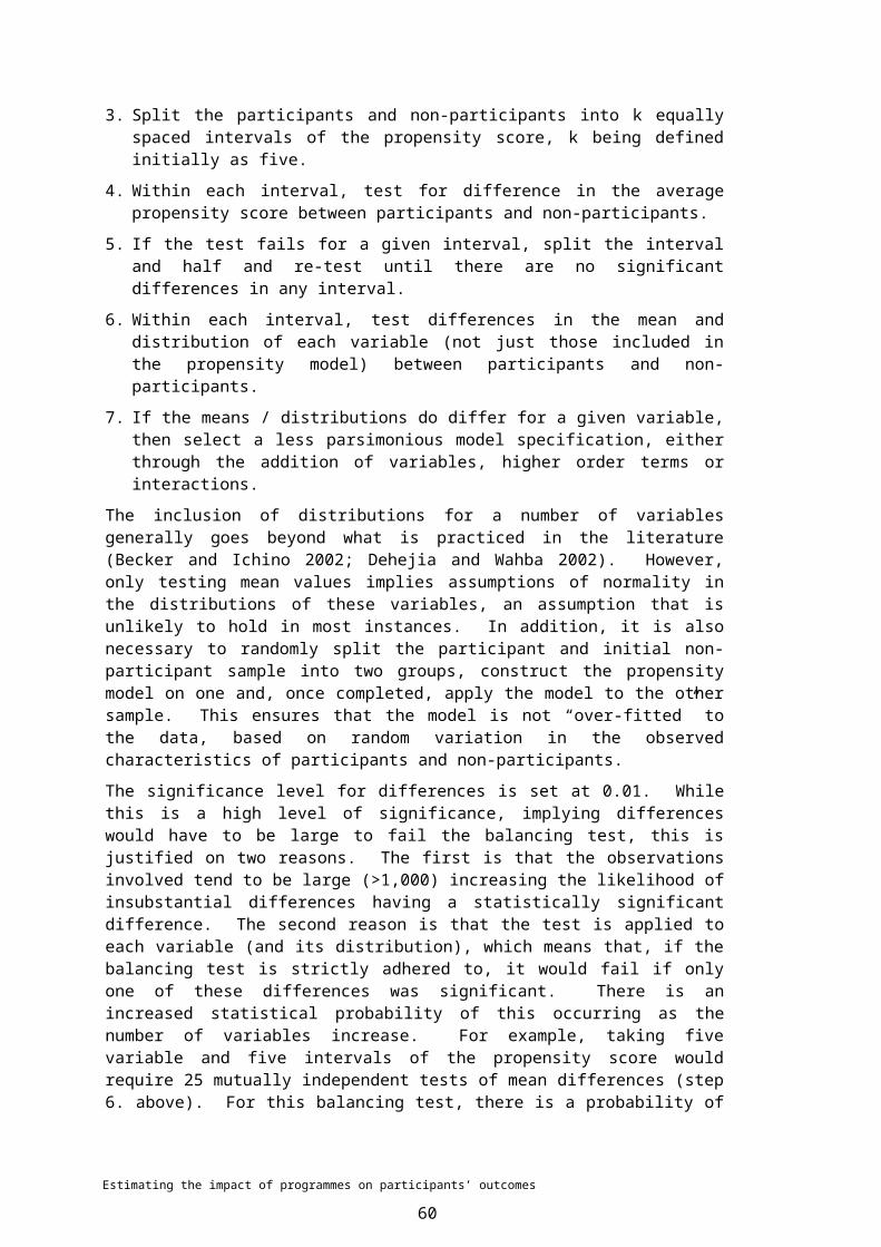
8 ConclusionsOver the last four years considerable progress has been made in the estimation of the impact of employment programmes on participants’ outcomes. The objective of measuring the impact of employment programmes has been achieved, with the current outcome measure independence of Work and Income assistance as well as the impact estimation technique - propensity matching allowing for ongoing and comprehensive monitoring of programme outcomes and impact. However, as has been pointed out in a number of sections, there are areas for improvement and further work.
Participation in employment programmesData quality is the most significant issue with programme participation. In the main, analysis of impact has been confined to those programmes where evaluators have a reasonable level of certainty that the participation did occur and that it is known what the person did; often limiting work to nationally prescribed programmes. The challenge is to be able extend the monitoring of programme impact to regionally delivered initiatives, where both data quality and programme size present greater challenges.
How programme participation is defined in the analysis has a significant bearing on what programme effect is being estimated. In particular, participation in the same or similar programmes in the period before starting a programme implies that the impact estimate measures the marginal gain of participating in the programme rather than an absolute effect.
Recommendations:
1. Continue to lobby for the maintenance of robust and transparent systems of recording programme participation within the administrative datasets. One immediate area will be the need to develop IAP business rules in the extraction of information from Conquest (contract management database) as well as the linkages this information has to programme information recorded in SOLO.
2. Document programme information that exists outside the administrative databases. For example, ensure that institutional knowledge about different types of employment programmes is retained so that it will be possible to compare the impacts of current programmes with similar programmes in the past.
3. Examine how programme duration and participation sequences affect estimates of programme impact.
Observable characteristicsThe number of observable characteristics, especially those linked to either outcomes or programme participation significantly decreases the problem of unobserved selection bias. Not surprisingly, the availability of rich datasets reduces the level of unknown information about individual’s propensity to participate in programmes or achieve an outcome. Moreover, the greater the number of relevant characteristics observed the more chance that unobserved factors will at least be indirectly represented. For example, previous labour market outcomes provide a good indication of possible future outcomes.
Estimating the impact of programmes on participants’ outcomes
60

Like programme participation, there are also data quality issues associated with the characteristics of people recorded in administrative databases. Improving the quality as well as the range of information on people will continue to be an important goal in improve impact estimates.
Recommendations:
1. Continue to lobby for the maintenance of robust and transparent systems of recording information on client characteristics, especially those that are known to influence people’s labour market outcomes.
2. Continue to increase the number of characteristics that can be used in analysis of impact. For example, investigate the quality of SWIFTT information on previous income / labour market status before applying for benefit or the level of Work and Income debt that a client may have.
Outcome measuresThe current measure of independence of Work and Income assistance is considered to be robust and unbiased, but has several limitations. Not least of which is the possibility that it only approximates labour market outcomes and employment in particular. This imposes the assumption that any change in the probability of being independent of Work and Income assistance through a programme reflects an underlying change in the probability of being in employment or training rather than other, possibly negative, outcomes.
The way in which outcomes are specified has considerable bearing on the estimated impact of the programme. In particular, the measuring outcomes at “points in time” versus “cumulative” will lead to different conclusions depending on the time frame used. Which specification is used will depend on the evaluation question, for example, point in time measures provide a clear perspective on the changing outcomes and impact of programmes over time, while cumulative measures are appropriate in determining the overall benefit of the programme to participants.
Recommendation:
1. There is limited opportunity to improve the current outcome measure with available administrative data other than to include data on the receipt of Student Loans and Allowances. This makes the integration of MSD administrative data with IRD information a priority. IRD information is outcome rich in that it records people’s monthly income and earnings if employed or annual income from those self-employed. This will not only provide direct confirmation of employment outcomes, but also measures of wage levels and firm/industry data. This latter information is invaluable for any further analysis of the likely macroeconomic effect is of these programmes, especially around substitution and displacements effects.
Impact estimationsBased on overseas analysis, it would appear that, in the New Zealand context, current approaches to estimating programme impact are able to account for three of the four major sources of selection bias. This provides some confidence that the resulting impact estimates are at least reliable in terms of sign and magnitude. However, both propensity matching and outcomes regression hold the same key assumption, namely that unobserved differences between participants and non-
Estimating the impact of programmes on participants’ outcomes
61
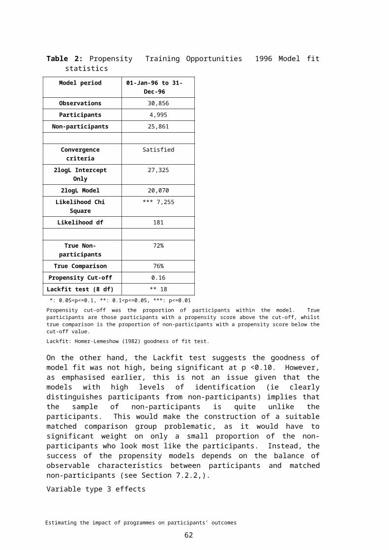
participants are not important in determining outcomes in the absence of participation in the programme. It is unlikely that this assumption is true. Instead the question is to what extent has the assumption been violated and as a result to what extent the estimates differ from the programme’s true impact.
Another message to come from the international literature is that there is no one method for determining programme impact. The appropriateness or otherwise of methods depends on the particular programme context and the information that is available to evaluators. For example, while propensity matching is the current standard approach it is important to ensure that the assumptions that underlie it remain valid.
Recommendations:
1. Conduct a systematic analysis to determine the completeness of administrative data in capturing those variables that influence labour market outcomes. This will facilitate the identification of areas of weakness (for example, the importance of not having income histories, in constructing matched groups of non-participants).
2. Need to develop tests of the assumptions of different estimation techniques.
3. Develop estimators that control for unobserved differences between participants and non-participants.
4. Consider conducting an experimental design of an employment programme to provide an opportunity to test the relative performance of experimental and non-experimental impact estimators. The purpose of this is to help improve our knowledge of non-experimental estimators rather than as a contest between the two approaches, given the difficulty and cost of conducting experimental designs on an ongoing basis.
Closing remarksIt is perhaps important at this point to reiterate the points made at the start of the paper. The issues discussed here apply to only one part of the broader question of programme effectiveness. Estimates of the impact programmes have on non-participants are as important in assessing programme effectiveness as the issues covered in this paper. Unfortunately the balance in the literature, both here and internationally, has been concerned with the accurate estimation of programmes impact on participant outcomes. While important, achievement of such accurate estimates may provide a false sense of security to decision makers in that they have an “answer” and place too much weight on its robustness rather than what it can tell about the programmes’ overall effectiveness. Conversely, it is important not to allow uncertainty around impact estimates to lead to indecision, for example, discounting impact estimates on the unknown level of selection bias. Uncertainty is an ever present reality in the policy and evaluation and simply needs to be included as part of any decision making process.
Related to the need to place this empirical analysis within a broader theoretical framework of programme effectiveness is the importance of other evaluative methods in helping to understand why programmes have the impacts that they do. Counterfactual designs have very little to say about the actual interaction between participants, their context and the programme or intervention. Unpacking the “black box” is a necessary complement to any findings over programme impact to provide useful information for decision making, as on its own, impact estimates give no guidance as to what decision makers might sensibly do next.
Estimating the impact of programmes on participants’ outcomes
62

ReferencesAshenfelter Orley, , "Estimating the Effect of Training on Earnings", Review of Economics and Statistics 60: 47-57, 1978.
Ashenfelter Orley and Card David (1985) “Using the longitudinal structure of earnings to estimate the effect of training programmes” Review of Economics and Statistics 67(4): 648-60, 1985..
Becker Sascha, and Ichino Andrea, “Estimation of the average treatment effect based on propensity scores” The Stata Journal 2(4): 358-77, 2002..
Bloom Howard, “Using non-experimental methods to estimate program impacts: statistical models, matches and muddles” University of California at Berkeley Seminar Series Evaluating Welfare Reform: Non-Experimental Approaches, 2002.
Bloom Howard; Michalopoulos Charles; Hill Carolyn; and Lei Ying, Can Nonexperimental Comparison Group Methods Match the Findings from a Random Assignment Evaluation of Mandatory Welfare-To-Work Programmes, MDRC Working Papers on Research Methodology, Manpower Demonstration Research Corporation, New York, 2002.
Bryson Alex; Dorestt Richard; and Purdon Susan, The Use of Propensity Score Matching in the Evaluation of Active Labour Market Policies, Working Paper No 4, Department of Work and Pensions, London, 2002.
Calmfors Lars, “Active labour market policy and unemployment a framework for the analysis of crucial design features”, Labour Market and Social Policy Occasional Papers No. 15, OECD, Paris, 1994.
Chapple Simon, “Displacement effects of active labour market policy”, New Zealand Department of Labour Occasional Paper 1997/3, Labour Market Policy Group, Department of Labour, Wellington, 1997.
de Boer Marc, Review of the Subsidised Work Appropriation: Method Paper, Ministry of Social Development, Wellington, 2002.
de Boer Marc, Effectiveness of New Zealand Employment Programmes: Theory and Evidence, Employment Evaluation Working Paper 2003/4 (draft), Department of Labour and Ministry of Social Development, Wellington, 2003a.
de Boer Marc, Re-Assessment of the Impact of Work Track Pilot Programme on Participants’ Outcomes, Employment Evaluation Working Paper 2003/2 (draft), Department of Labour and Ministry of Social Development, Wellington, 2003b.
Dehejia Rajeev and Wahba Sadek, “Causal effects of non-experimental studies: re-evaluating the evaluation of training programs”, Journal of the American Statistical Association 99:448: 1053-62, 1999.
Dehejia Rajeev and Wahba Sadek, “Propensity score-matching methods for non-experimental causal studies”, Review of Economic and Statistics 84(1): 151-61, 2002
Department of Employment, Education, Training and Youth Affairs (DEETYA), The Net Impact of Labour Market Programmes: Improvements in the Employment Prospects of Those Assisted, EMB Report 2/97, Analysis and Evaluation Division, Canberra, 1997.
Dockery Alfred. M and Stromback Thorsten, Evaluation of Labour Market Programs: An Assessment, Paper prepared for the 29th Annual Conference of Economists, Gold Coast, Australia, 3-6 July 2000.
Estimating the impact of programmes on participants’ outcomes
63
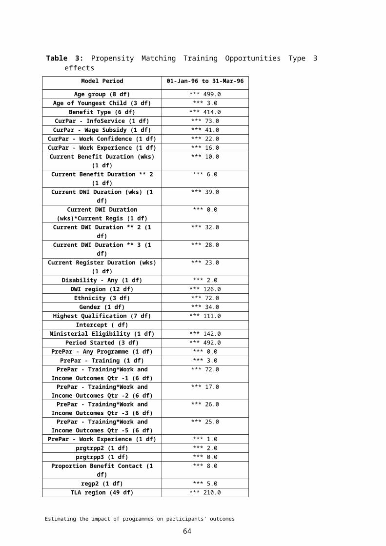
Friedlander D and Robins P K, “Evaluating program evaluations: new evidence on commonly used nonexperimental methods”, American Economic Review 85(4): 923-37, 1995.
Glazerman Steven; Levy Dan; and Myers David, Non-Experimental Replication of Social Experiments: A Systematic Review (Interim Report), Mathematics Policy Research, Inc. Reference No: 8813-300, Dallas, Texas, 2002.
Heckman James; and Hotz Joseph, “Choosing among alternative nonexperimental methods of estimating the impact of social programmes: the case of manpower training”, Journal of the American Statistical Association 84(408): 862-74, 1989
Heckman James; Ichimura Hidehiko; and Todd Petra “Matching as an econometric evaluation estimator: evidence from evaluating a job training programme” Review of Economic Studies 64: 605-54, 1997.
Heckman James; LaLonde Robert; and Smith, Jeffrey, “The economics and econometrics of active labour market programmes” in Ashenfelter, O. and Card, D. Handbook of Labour Market Economics Vol 3a, Amsterdam, 1999.
Heckman James; and Smith Jeffrey, “The pre-program earnings dip and the determinants of participation in a social program: implications for simple program evaluation strategies”, Economic Journal 109(457): 313-48, 1999.
Heckman James; Heinrich Carolyn; and Smith Jeffrey, The Performance of Performance Standards, NBER Working Paper No. w9002, June 2002.
LaLonde Robert, “Evaluating the econometric evaluation of training programs with experimental data”, American Economic Review, 76(4): 604-20, 1986.
Maré David, “What works for whom?: the effectiveness of different employment programmes”, Proceedings of the Ninth Conference of Labour, Employment and Work in New Zealand, ed. Morrison, Philip., Victoria University of Wellington. 2000.
Ministry of Social Development, The Impact, Locking-in Effect and Post-participation Effect of Community Work Experience Programmes, February 2003 Report on MSD employment programme effectiveness and risk (Appendix 5 Purchase Agreement), 2003.
Rosenbaum Paul; and Donald Rubin, “The central role of the propensity score in observational studies of causal effects”, Biometrika 70(1): 41-55, 1983
Sianesi Barbara, An Evaluation of the Active Labour Market Programmes in Sweden, IFAU Working Paper 2001:5, IFAU – Office of Labour Market Policy Evaluation, Uppsala, 2001.
Swindells James, Evaluation Report for the Work Track Programme, Centre for Operational Research and Evaluation, Department of Work and Income, Wellington, 2000.
Smith Jeffery; and Todd Petra, Does Matching Overcome LaLonde’s Critique of Nonexperimental Estimators? 2000. Downloadable from http://www.bsos.und.edu/econ/jsmith?/paper.html.
Estimating the impact of programmes on participants’ outcomes
64
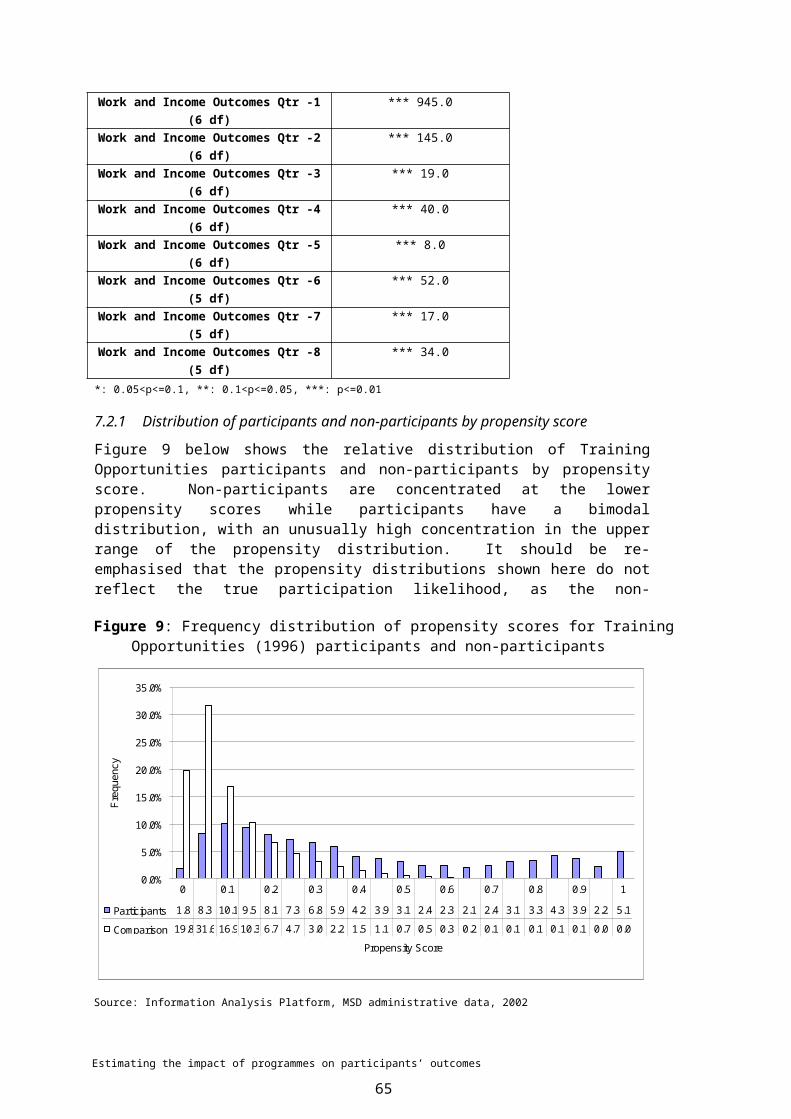
Appendix 1: Alternative propensity model specificationsIn developing the propensity matching approach the initial model specification was based on the backward selection of significant main effects and interactions. This approach has been replaced with the use of the balancing test to determine the propensity model. The following examines the effect of these two approaches on the observed bias between participants and non-participants as well a on the subsequent estimates of programme impact.
Table 10 compares the proportion of participants for which observed characteristics are balanced between participants and non-participants conditional on propensity score a well as the mean difference in observed bias between participants and non-participants. In the main, using the balancing test approach produces a better balance between participants and matched non-participants. Similarly, the mean observed bias between participants and non-participants is also smaller, but not in all cases.
Table 10: Observed bias and balance between Training Opportunities (1998) participants and matched comparison group using two alternative model specifications
Model selection Procedure
Balance Test Backward Selection
Variable ClassBalance (% of participants)
Observed Bias
Balance (% of participants)
Observed Bias
Ethnicity European 100% -3.2 % 96% -3.8 %
Maori 100% 0.8 % 100% 2.9 %
Pacific People 84% 0.4 % 100% 0.7 %
Other 98% 2.0 % 100% 0.2 %
Gender Female 100% -0.4 % 100% 3.5 %
Male 100% 0.4 % 100% -3.5 %
Age in years (blank) 100% -0.57 yr 100% -1.88 yr
Age group 15-17 yr 80% 2.8 % 66% 6.4 %
18-19 yr 91% -1.7 % 87% 5.0 %
20-24 yr 94% -1.4 % 81% -2.5 %
25-29 yr 96% 1.7 % 87% -3.5 %
30-39 yr 99% 0.0 % 100% -2.6 %
40-49 yr 97% -0.9 % 100% -1.1 %
50-54 yr 100% -0.7 % 100% -1.2 %
55-59 yr 100% 0.1 % 100% -0.4 %
60+ yr 100% 0.0 % 100% -0.1 %
Disability - Any Yes 100% -0.2 % 100% 0.0 %
Disability - Intellect Yes 100% 0.4 % 70% 0.8 %
Disability - Mental Yes 100% 0.1 % 100% -0.1 %
Disability - Physical Yes 100% -0.4 % 100% -0.6 %
Disability - Sensory Yes 100% 0.0 % 100% 0.2 %
Language & Numeracy Yes 88% 1.5 % 100% 0.3 %
Drug & Alcohol Yes 100% 0.0 % 100% -0.2 %
Refugee Yes 100% 0.4 % 94% 0.2 %
Highest Qualification None 100% -1.3 % 100% -0.5 %
School Certificate 100% 0.8 % 100% 1.6 %
Secondary above SC 93% 0.1 % 100% -1.0 %
Post School 100% 0.5 % 90% -0.1 %
Ministerial Eligibility Not Eligible 82% 6.2 % 100% 9.5 %
Estimating the impact of programmes on participants’ outcomes
65

Model selection Procedure
Balance Test Backward Selection
Variable ClassBalance (% of participants)
Observed Bias
Balance (% of participants)
Observed Bias
26+weeks 82% -6.2 % 100% -9.5 %
SGI group SGI 99 91% 1.4 % 96% 2.5 %
SGI 1 100% -0.2 % 100% 0.0 %
SGI 2 100% -1.5 % 100% -1.2 %
SGI 3 32% -0.2 % 96% -0.8 %
SGI 4 100% 0.5 % 100% -0.6 %
SGI 5 100% -0.1 % 100% 0.0 %
SGI score (blank) 91% -1.19 pnts 96% -1.68 pnts
Partner Yes 98% 0.0 % 100% -2.7 %
Number of Children None 100% -0.6 % 100% 1.8 %
1 Child 97% -0.3 % 100% -1.0 %
2+ Child 100% 1.0 % 84% -0.8 %
Age of Youngest Child No Child 100% -0.6 % 100% 1.8 %
0-5 yr 100% 0.6 % 100% -0.6 %
6-13 yr 98% 1.1 % 100% -0.3 %
14+ yr 100% -1.1 % 100% -0.9 %
CurPar - Any Programme Yes 0% 91.7 % 0% 92.6 %
CurPar - InfoService Yes 100% 0.5 % 100% 0.2 %
CurPar - Into Work Yes 100% -0.1 % 100% 0.0 %
CurPar - Job Search Yes 100% 0.2 % 100% -0.1 %
CurPar - Other Yes 100% 0.0 % 100% 0.0 %
CurPar - Training Yes 0% 100.0 % 0% 100.0 %
CurPar - Wage Subsidy Yes 46% -0.6 % 100% -0.4 %
CurPar - Work Confidence Yes 100% 0.0 % 85% 1.0 %
CurPar - Work Experience Yes 100% -0.7 % 100% -0.8 %
PrePar - Any Programme (blank) 93% -0.42 days 50% 19.35 days
PrePar - Job Search (blank) 100% 0.12 days 100% 0.07 days
PrePar - Other (blank) 100% 0.00 days 100% 0.00 days
PrePar - Training (blank) 41% 1.74 days 59% 19.17 days
PrePar - Wage Subsidy (blank) 100% -1.05 days 100% -0.58 days
PrePar - Work Confidence (blank) 100% -0.16 days 100% 0.89 days
PrePar - Work Experience (blank) 100% -1.06 days 100% -0.20 days
Benefit Type Unemployment 100% -0.3 % 100% -0.2 %
Independent Youth 83% -0.3 % 100% 0.4 %
Domestic Purposes 98% 0.0 % 100% -0.8 %
Emergency 98% 0.6 % 100% 0.1 %
Invalids 100% 0.1 % 100% 0.2 %
Sickness 100% -0.2 % 100% 0.2 %
Current Benefit Duration (wks) (blank) 93% -6.82 wks 100% -9.54 wks
Current Benefit Duration 0-13 wks 44% -1.5 % 84% 1.8 %
14-25 wks 100% 1.1 % 89% -0.3 %
26-51 wks 71% -0.4 % 100% -1.8 %
52-103 wks 98% 2.5 % 100% 2.7 %
104-207 wks 100% -0.2 % 100% -0.3 %
208+ wks 98% -1.6 % 100% -2.2 %
Proportion Benefit Contact (blank) 93% -2.57 pnts 100% -3.66 pnts
Current DWI Duration (wks) (blank) 93% -7.50 wks 100% -16.43 wks
Current DWI Duration 0-13 wks 42% -1.8 % 84% 0.3 %
14-25 wks 97% 0.8 % 89% 0.4 %
26-51 wks 96% 0.2 % 100% -0.3 %
Estimating the impact of programmes on participants’ outcomes
66
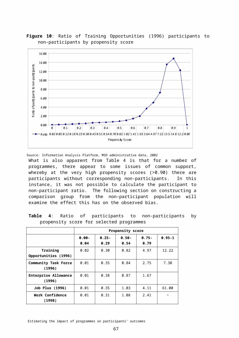
Model selection Procedure
Balance Test Backward Selection
Variable ClassBalance (% of participants)
Observed Bias
Balance (% of participants)
Observed Bias
52-103 wks 79% 1.9 % 100% 3.2 %
104-207 wks 100% 0.9 % 72% -0.5 %
208+ wks 91% -2.0 % 100% -3.1 %
Proportion DWI Contact (blank) 93% -2.57 pnts 100% -3.66 pnts
Current Register Duration (wks) (blank) 100% -6.70 wks 100% -11.48 wks
Current Register Duration 0-13 wks 47% 5.2 % 100% 10.9 %
14-25 wks 83% 1.0 % 100% -1.4 %
26-51 wks 99% -3.2 % 100% -3.6 %
52-103 wks 99% -1.4 % 100% -3.2 %
104-207 wks 100% -0.1 % 100% -1.3 %
208+ wks 44% -1.5 % 100% -1.3 %
Proportion Work Contact (blank) 68% -3.35 pnts 80% -3.59 pnts
Work and Income Outcomes Qtr -1Independent of Work and Income 96% 2.2 % 84% 3.6 %
Dependent on Work and Income 100% -10.2 % 100% -19.1 %
Training 96% 8.6 % 90% 14.1 %
Job Search 100% 0.2 % 100% -0.1 %
Wage Subsidy 100% -0.1 % 100% 0.3 %
Work Confidence 44% 0.1 % 100% 1.7 %
Work Experience 100% -0.8 % 100% -0.3 %
Other Programme 100% 0.0 %
Work and Income Outcomes Qtr -2Independent of Work and Income 87% 0.6 % 84% 1.0 %
Dependent on Work and Income 100% -5.8 % 100% -14.0 %
Training 100% 6.1 % 84% 12.1 %
Job Search 100% 0.1 % 100% -0.3 %
Wage Subsidy 100% -0.3 % 84% -0.2 %
Work Confidence 100% 0.0 % 76% 1.6 %
Work Experience 100% -0.8 % 84% -0.2 %
Other Programme 100% 0.0 %
Work and Income Outcomes Qtr -3Independent of Work and Income 87% 1.2 % 100% 0.7 %
Dependent on Work and Income 100% -5.3 % 100% -11.7 %
Training 100% 4.4 % 76% 10.1 %
Job Search 100% 0.5 % 84% -0.4 %
Wage Subsidy 100% -0.4 % 79% 0.1 %
Work Confidence 100% 0.1 % 100% 1.4 %
Work Experience 93% -0.5 % 84% -0.2 %
Work and Income Outcomes Qtr -4Independent of Work and Income 90% 0.7 % 84% 0.6 %
Dependent on Work and Income 100% -2.0 % 100% -8.9 %
Training 100% 2.3 % 76% 8.1 %
Job Search 100% -0.2 % 96% -0.2 %
Wage Subsidy 100% -0.4 % 100% 0.1 %
Work Confidence 100% 0.2 % 100% 0.5 %
Work Experience 100% -0.5 % 84% -0.1 %
Work and Income Outcomes Qtr -5Independent of Work and Income 92% 1.5 % 84% 0.3 %
Dependent on Work and Income 93% -1.6 % 100% -7.2 %
Training 91% 1.1 % 100% 6.5 %
Estimating the impact of programmes on participants’ outcomes
67

Model selection Procedure
Balance Test Backward Selection
Variable ClassBalance (% of participants)
Observed Bias
Balance (% of participants)
Observed Bias
Job Search 100% -0.1 % 84% -0.2 %
Wage Subsidy 100% -0.2 % 100% -0.3 %
Work Confidence 100% -0.3 % 100% 1.0 %
Work Experience 100% -0.3 % 84% -0.2 %
Work and Income Outcomes Qtr -6Independent of Work and Income 84% 2.9 % 100% 0.7 %
Dependent on Work and Income 93% -2.4 % 100% -6.5 %
Training 100% 0.3 % 100% 5.9 %
Wage Subsidy 100% -0.1 % 100% -0.4 %
Work Confidence 100% -0.6 % 100% 0.0 %
Work Experience 100% -0.1 % 100% 0.3 %
Work and Income Outcomes Qtr -7Independent of Work and Income 84% 3.2 % 100% 2.1 %
Dependent on Work and Income 100% -2.2 % 100% -7.9 %
Training 100% 0.1 % 100% 5.6 %
Wage Subsidy 100% -0.4 % 100% -0.2 %
Work Confidence 100% -0.4 % 84% 0.4 %
Work Experience 100% -0.2 % 100% 0.0 %
Work and Income Outcomes Qtr -8Independent of Work and Income 93% 3.1 % 76% 3.6 %
Dependent on Work and Income 100% -2.3 % 100% -8.2 %
Training 100% -0.4 % 100% 5.5 %
Job Search 100% -0.2 % 100% -0.3 %
Wage Subsidy 100% -0.3 % 100% -0.3 %
Work Confidence 100% 0.2 % 100% -0.4 %
Work Experience 100% 0.0 % 100% 0.1 %
Period Started 1998/1 82% 5.6 % 100% 8.7 %
1998/2 97% -2.3 % 100% -3.0 %
1998/3 93% -1.0 % 84% -1.9 %
1998/4 100% -2.3 % 100% -3.8 %
DWI region Auckland Central 100% -0.3 % 100% 0.4 %
Auckland North 98% 0.9 % 100% -0.2 %
Auckland South 97% -0.2 % 100% -0.3 %
Bay of Plenty 98% -0.8 % 100% -0.7 %
Canterbury 96% -0.3 % 100% -1.0 %
Central 100% 0.3 % 96% -0.4 %
East Coast 96% 0.1 % 100% 1.3 %
Nelson 100% -0.1 % 100% 0.6 %
Northland 100% -0.5 % 100% -0.2 %
Southern 96% 0.3 % 100% 0.9 %
Taranaki 100% -0.4 % 100% -0.1 %
Waikato 89% -0.4 % 100% -0.8 %
Wellington 87% 1.3 % 79% 0.4 %
The effect of alternative propensity model selection has on the subsequent estimations of programme impact are shown in and Figure 14. The use of backward selection () produces larger pre-participation outcome differences than the balancing test approach, while the estimated impact of Training Opportunities using backward selection is higher than using the balancing test approach. The lower observed bias using the balancing test would indicate that the impact estimates derived through this
Estimating the impact of programmes on participants’ outcomes
68
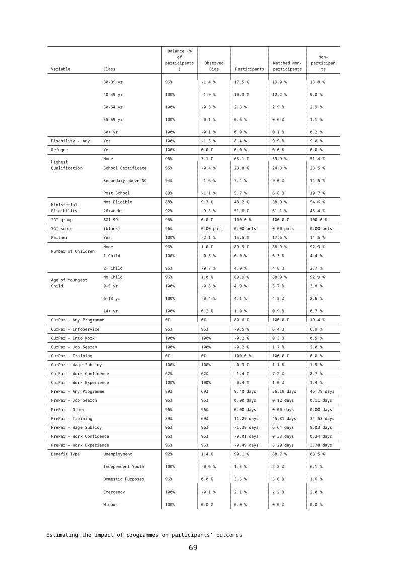
approach are more accurate than the use of backward selection. However, in this particular instance, both estimates would produce very similar conclusions over the impact of this programme.
Figure 13: Independence of Work and Income assistance among Training Opportunities (1998) participants and propensity (backward selection) matched comparison group
0%
10%
20%
30%
40%
50%
60%
-12 -9 -6 -3 0 3 6 9 12 15 18 21 24 27 30 33 36 39 42 45 48 51
Inde
pend
ent o
f W&
I Ass
istan
ce
Participants ComparisonBase: 4,937 participants at participation start
Lapse period from participation start (Months)
Figure 14: Independence of Work and Income assistance among Training Opportunities (1998) participants and propensity (balancing test) matched comparison group
0%
10%
20%
30%
40%
50%
60%
-12 -9 -6 -3 0 3 6 9 12 15 18 21 24 27 30 33 36 39 42 45 48 51
Inde
pend
ent o
f W&
I Ass
istan
ce
Participants ComparisonBase: 4,921 participants at participation start
Lapse period from participation start (Months)
Appendix 2: Summary of propensity logistic model
Estimating the impact of programmes on participants’ outcomes
69
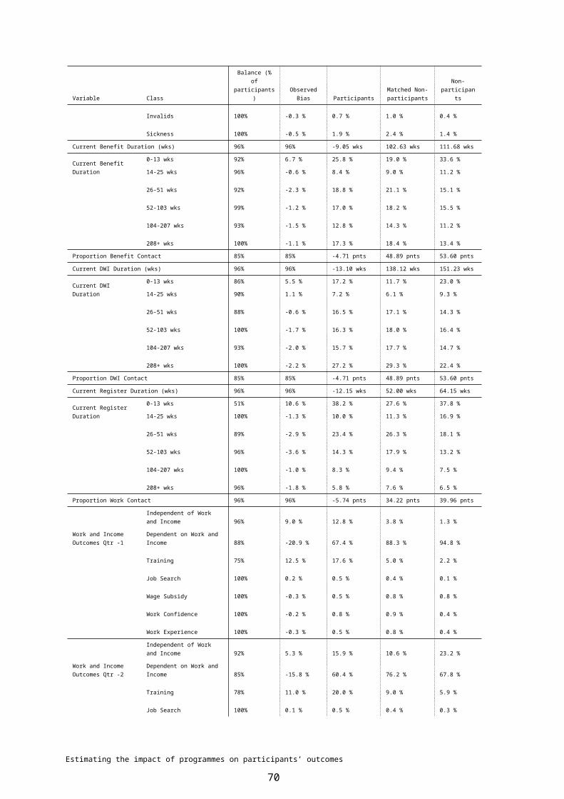
Table 11: Beta variable standard errors, chi-square and p values for the propensity model of participation in Training Opportunities (1996).
Model Period Class 1 Class 2p value, estimate (standard error)
Age group (Ref: 20-25 yr) 15-17 yr *** 1.36 (0.08)
18-19 yr *** -0.3 (0.06)
25-29 yr *** 0.42 (0.07)
30-39 yr *** 0.41 (0.06)
40-49 yr *** 0.32 (0.07)
50-54 yr -0.07 (0.12)
55-59 yr * -0.37 (0.21)
60+ yr -0.8 (0.62)
Age of Youngest Child (Ref: No Child) 0-5 yr 0.08 (0.09)
6-13 yr ** 0.22 (0.1)
14+ yr 0.14 (0.18)
Benefit Type (Ref: Unemployment) Invalids *** 0.75 (0.21)
Sickness ** 0.34 (0.14)
Widows * 1.29 (0.74)
Domestic Purpose *** 0.87 (0.13)
Eemergency -0.07 (0.14)
Independent Youth *** -2.73 (0.15)
CurPar - InfoService (Ref: No) Yes *** 0.66 (0.07)
CurPar - Wage Subsidy (Ref: No) Yes *** -0.84 (0.15)
CurPar - Work Confidence (Ref: No) Yes *** 0.43 (0.07)
CurPar - Work Experience (Ref: No) Yes *** -0.66 (0.17)
Current Benefit Duration (wks) (Ref: Continuous) - ** 0 (0)
Current Benefit Duration ** 2 (Ref: -) - ** 0 (0)
Current DWI Duration (wks) (Ref: Continuous) - *** 0 (0)
Current DWI Duration (wks)*Current Regis (Ref: Continuous | Continuous) - * 0 (0)
Current DWI Duration ** 2 (Ref: Continuous) - ** 0 (0)
Current DWI Duration ** 3 (Ref: Continuous) - * 0 (0)
Current Register Duration (wks) (Ref: Continuous) - *** 0 (0)
Disability - Any (Ref: No) Yes -0.01 (0.07)
DWI region (Ref: Auckland Central) Northland 0.19 (0.13)
Auckland North -0.04 (0.57)
Auckland South -0.17 (0.17)
Waikato ** 0.67 (0.23)
Central 0.21 (0.3)
Bay of Plenty -0.33 (0.2)
East Coast 0.33 (0.21)
Taranaki ** 0.38 (0.13)
Wellington *** 3.3 (0.37)
Nelson ** 0.67 (0.24)
Canterbury -0.2 (0.33)
Southern -0.03 (0.28)
Ethnicity (Ref: European) Maori *** 0.22 (0.05)
Estimating the impact of programmes on participants’ outcomes
70

Model Period Class 1 Class 2p value, estimate (standard error)
Other *** 0.78 (0.09)
Pacific People *** 0.4 (0.07)
Gender (Ref: Male) Female *** 0.19 (0.04)
Highest Qualification (Ref: None) Less than 3 SC p -0.06 (0.05)
3+ SC passes *** -0.37 (0.08)
SFC, UE or equiv *** -0.4 (0.08)
Scold, Bursary, H *** -0.88 (0.15)
Other school qua -0.08 (0.16)
Post school qual ** -0.29 (0.09)
Degree/Prof qual *** -0.88 (0.11)
Intercept (Ref: i) - *** -1.38 (0.14)
Ministerial Eligibility (Ref: Not Eligible) 26+weeks *** 0.84 (0.06)
Period Started (Ref: 1996qtr1) 1996/1 *** 1.47 (0.07)
1996/2 *** 0.67 (0.07)
1996/3 *** 1.04 (0.07)
PrePar - Any Programme (Ref: No) - 0 (0)
PrePar - Training (Ref: No) - ** 0.01 (0)
PrePar - Training*Work and Income Outcomes Qtr -1 (Ref: No | Independent W_I)
Training *** -0.01 (0)
Dependent on Work and Income 0 (0)
Work Confidence 0 (0)
Work Experience 0 (0.01)
Wage Subsidy ** 0.01 (0)
Job Search 0 (0.01)
PrePar - Training*Work and Income Outcomes Qtr -2 (Ref: No | Independent W_I)
Training ** 0 (0)
Dependent on Work and Income * 0 (0)
Work Confidence 0 (0)
Work Experience 0 (0)
Wage Subsidy 0 (0)
Job Search 0 (0)
PrePar - Training*Work and Income Outcomes Qtr -3 (Ref: No | Independent W_I)
Training *** 0 (0)
Dependent on Work and Income *** 0 (0)
Work Confidence 0 (0)
Work Experience 0 (0)
Wage Subsidy ** -0.01 (0)
Job Search 0 (0)
PrePar - Training*Work and Income Outcomes Qtr -5 (Ref: No | Independent W_I)
Training ** 0 (0)
Dependent on Work and Income *** 0 (0)
Work Confidence 0 (0)
Work Experience *** -0.01 (0)
Wage Subsidy 0 (0)
Job Search -0.01 (0.01)
PrePar - Work Experience (Ref: No) - 0 (0)
prgtrpp2 (Ref: -) - 0 (0)
prgtrpp3 (Ref: -) - 0 (0)
Proportion Benefit Contact (Ref: Percent 0) - ** 0 (0)
regp2 (Ref: -) - ** 0 (0)
Estimating the impact of programmes on participants’ outcomes
71

Model Period Class 1 Class 2p value, estimate (standard error)
TLA region (Ref: Auckland City) Waikato ** -0.77 (0.27)
Ashburton * 0.7 (0.4)
Buller -0.22 (0.31)
Central Hawkes B -0.41 (0.43)
Central Otago -0.38 (0.52)
Christchurch Cit 0.1 (0.33)
Clutha 0.32 (0.44)
Dunedin City 0.37 (0.29)
Far North * -0.29 (0.16)
Franklin 0.31 (0.27)
Gisborne -0.05 (0.22)
Gore 0.65 (0.4)
Grey -0.05 (0.28)
Hamilton City ** -0.76 (0.24)
Hastings ** -0.48 (0.23)
Hauraki * -0.52 (0.29)
Horowhenua 0.08 (0.34)
Hutt City *** -3.14 (0.38)
Invercargill Cit 0.05 (0.3)
Kaipara 0.23 (0.27)
Kapiti Coast -0.44 (0.38)
Kawerau ** 0.57 (0.27)
Manawatu -0.14 (0.38)
Manukau City * 0.28 (0.17)
Marlborough -0.12 (0.28)
Masterton -0.48 (0.34)
Matamata-Piako -0.61 (0.4)
Napier City -0.34 (0.23)
Nelson City -0.16 (0.27)
New Plymouth -0.17 (0.15)
North Shore City 0.46 (0.59)
Opotiki * 0.52 (0.27)
Palmerston North 0.11 (0.32)
Papakura 0.2 (0.22)
Porirua City *** -3.06 (0.38)
Rodney 0.66 (0.61)
Rotorua ** 0.59 (0.21)
Ruapehu -0.17 (0.22)
South Taranaki -0.29 (0.25)
South Waikato 0.37 (0.24)
Tararua *** 0 ()
Estimating the impact of programmes on participants’ outcomes
72
Model Period Class 1 Class 2p value, estimate (standard error)
Tasman *** 0 ()
Taupo 0.22 (0.27)
Tauranga 0.32 (0.22)
Thames-Coromande ** -1.14 (0.37)
Timaru 0.08 (0.31)
Upper Hutt City *** -3.91 (0.44)
Waimakariri *** 0 ()
Waipa *** 0 ()
Wairoa *** 0 ()
Waitakere City 0.28 (0.57)
Waitaki *** 0 ()
Waitomo 0.12 (0.27)
Wanganui *** 0 ()
Wellington City *** -3.39 (0.38)
Whakatane *** 0 ()
Whangarei *** 0 ()
Stratford -0.28 (1.35)
Work and Income Outcomes Qtr -1 (Ref: Independent W_I) Training *** -0.82 (0.16)
Dependent on Work and Income *** -3.03 (0.1)
Work Confidence *** -3.43 (0.21)
Work Experience *** -2.89 (0.32)
Wage Subsidy *** -3.73 (0.33)
Job Search *** -2.09 (0.27)
Work and Income Outcomes Qtr -2 (Ref: Independent W_I) Training *** 1.13 (0.16)
Dependent on Work and Income *** 0.98 (0.09)
Work Confidence *** 1.24 (0.19)
Work Experience ** 0.74 (0.28)
Wage Subsidy *** 0.95 (0.25)
Job Search *** 0.96 (0.26)
Work and Income Outcomes Qtr -3 (Ref: Independent W_I) Training ** 0.3 (0.15)
Dependent on Work and Income * 0.15 (0.08)
Work Confidence 0.27 (0.19)
Work Experience * 0.41 (0.24)
Wage Subsidy 0.32 (0.22)
Job Search -0.13 (0.27)
Work and Income Outcomes Qtr -4 (Ref: Independent W_I) Training 0.14 (0.11)
Dependent on Work and Income ** -0.22 (0.07)
Work Confidence -0.09 (0.2)
Work Experience ** -0.52 (0.23)
Wage Subsidy -0.07 (0.19)
Estimating the impact of programmes on participants’ outcomes
73
Model Period Class 1 Class 2p value, estimate (standard error)
Job Search * -0.52 (0.31)
Work and Income Outcomes Qtr -5 (Ref: Independent W_I) Training * 0.33 (0.17)
Dependent on Work and Income 0 (0.07)
Work Confidence 0.2 (0.26)
Work Experience ** 0.59 (0.25)
Wage Subsidy 0.15 (0.2)
Job Search -0.04 (0.5)
Work and Income Outcomes Qtr -6 (Ref: Independent W_I) Training 0.02 (0.11)
Dependent on Work and Income *** -0.49 (0.06)
Work Confidence 0.23 (0.26)
Work Experience -0.36 (0.25)
Wage Subsidy -0.16 (0.19)
Work and Income Outcomes Qtr -7 (Ref: Independent W_I) Training ** 0.23 (0.11)
Dependent on Work and Income -0.04 (0.07)
Work Confidence 0.23 (0.29)
Work Experience -0.3 (0.26)
Wage Subsidy -0.02 (0.2)
Work and Income Outcomes Qtr -8 (Ref: Independent W_I) Training *** 0.3 (0.09)
Dependent on Work and Income *** -0.39 (0.08)
Work Confidence -0.39 (0.33)
Work Experience 0.28 (0.22)
Wage Subsidy -0.03 (0.17)
*: 0.05<p<=0.1, **: 0.1<p<=0.05, ***: p<=0.01
Acknowledgements:The following people are thanked for their helpful comments on earlier drafts of this paper.
CSRE: Coreen Adamson, Sankar Ramasamy, and James Swindells.
LMPG: Sarah Critchon, Steven Stillman.
Motu research: Dave Maré.
Disclaimer: The views expressed in this paper are those of the author and do not necessarily reflect the official position of either the Ministry of Social Development or the Department of Labour.
Estimating the impact of programmes on participants’ outcomes
74