ESTIMATION OF THE CENTRAL MOMENTS OF A RANDOM...
20
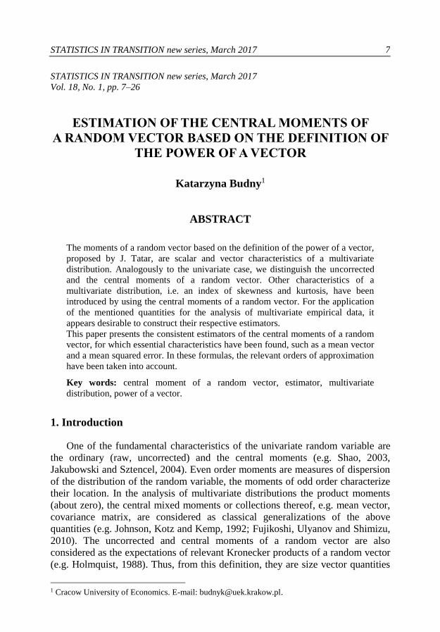
STATISTICS IN TRANSITION new series, March 2017 7 STATISTICS IN TRANSITION new series, March 2017 Vol. 18, No. 1, pp. 7–26 ESTIMATION OF THE CENTRAL MOMENTS OF A RANDOM VECTOR BASED ON THE DEFINITION OF THE POWER OF A VECTOR Katarzyna Budny 1 ABSTRACT The moments of a random vector based on the definition of the power of a vector, proposed by J. Tatar, are scalar and vector characteristics of a multivariate distribution. Analogously to the univariate case, we distinguish the uncorrected and the central moments of a random vector. Other characteristics of a multivariate distribution, i.e. an index of skewness and kurtosis, have been introduced by using the central moments of a random vector. For the application of the mentioned quantities for the analysis of multivariate empirical data, it appears desirable to construct their respective estimators. This paper presents the consistent estimators of the central moments of a random vector, for which essential characteristics have been found, such as a mean vector and a mean squared error. In these formulas, the relevant orders of approximation have been taken into account. Key words: central moment of a random vector, estimator, multivariate distribution, power of a vector. 1. Introduction One of the fundamental characteristics of the univariate random variable are the ordinary (raw, uncorrected) and the central moments (e.g. Shao, 2003, Jakubowski and Sztencel, 2004). Even order moments are measures of dispersion of the distribution of the random variable, the moments of odd order characterize their location. In the analysis of multivariate distributions the product moments (about zero), the central mixed moments or collections thereof, e.g. mean vector, covariance matrix, are considered as classical generalizations of the above quantities (e.g. Johnson, Kotz and Kemp, 1992; Fujikoshi, Ulyanov and Shimizu, 2010). The uncorrected and central moments of a random vector are also considered as the expectations of relevant Kronecker products of a random vector (e.g. Holmquist, 1988). Thus, from this definition, they are size vector quantities 1 Cracow University of Economics. E-mail: [email protected].
Transcript of ESTIMATION OF THE CENTRAL MOMENTS OF A RANDOM...
STATISTICS IN TRANSITION new series, March 2017
7
STATISTICS IN TRANSITION new series, March 2017
Vol. 18, No. 1, pp. 7–26
ESTIMATION OF THE CENTRAL MOMENTS OF
A RANDOM VECTOR BASED ON THE DEFINITION OF
THE POWER OF A VECTOR
Katarzyna Budny1
ABSTRACT
The moments of a random vector based on the definition of the power of a vector,
proposed by J. Tatar, are scalar and vector characteristics of a multivariate
distribution. Analogously to the univariate case, we distinguish the uncorrected
and the central moments of a random vector. Other characteristics of a
multivariate distribution, i.e. an index of skewness and kurtosis, have been
introduced by using the central moments of a random vector. For the application
of the mentioned quantities for the analysis of multivariate empirical data, it
appears desirable to construct their respective estimators.
This paper presents the consistent estimators of the central moments of a random
vector, for which essential characteristics have been found, such as a mean vector
and a mean squared error. In these formulas, the relevant orders of approximation
have been taken into account.
Key words: central moment of a random vector, estimator, multivariate
distribution, power of a vector.
1. Introduction
One of the fundamental characteristics of the univariate random variable are
the ordinary (raw, uncorrected) and the central moments (e.g. Shao, 2003,
Jakubowski and Sztencel, 2004). Even order moments are measures of dispersion
of the distribution of the random variable, the moments of odd order characterize
their location. In the analysis of multivariate distributions the product moments
(about zero), the central mixed moments or collections thereof, e.g. mean vector,
covariance matrix, are considered as classical generalizations of the above
quantities (e.g. Johnson, Kotz and Kemp, 1992; Fujikoshi, Ulyanov and Shimizu,
2010). The uncorrected and central moments of a random vector are also
considered as the expectations of relevant Kronecker products of a random vector
(e.g. Holmquist, 1988). Thus, from this definition, they are size vector quantities
1 Cracow University of Economics. E-mail: [email protected].

8 K. Budny: Estimation of the central …
(collections of product moments (about zero) and central mixed moments of the
corresponding orders).
On the basis of the definition of the power of a vector, Tatar (1996, 1999)
suggested multivariate generalizations of the uncorrected and the central moments
of a random variable, which are different from the above. Let us recall the basic
definitions.
Definition 1.1. [Tatar 1996, 1999] Let ,,, RH be a Hilbert space with the inner
product , . For any vector Hv and for any number 0 NNr the
r -th power of the vector v is defined as follows:
Rvo 1 and
evenfor,
oddfor
1
1
rvv
rvvv
r
r
r .
Let r
kL be a space of random vectors whose absolute value raised to the
r-th power has finite integral, that is:
dPRLrkr
k XX :: .
In the literature, the measure
dPErr
XX is sometimes called the
moment of the order r of a random vector X and designated as rE X (see
Bilodeau and Brenner, 1999). Tatar (2002), however, by analogy with the
univariate case, defines this expression as the absolute moment of order r of a
random vector X . In this study, we will also regard these values as the absolute
moments of a random vector.
Therefore, let us assume that for the vector kR:X an absolute moment
of order r exists.
Definition 1.2. [Tatar 1996, 1999] The ordinary (raw, uncorrected) moment of
order r of the random vector kR:X is defined as
rkr E X, . 1.1
Let us note that the uncorrected moment of the first order is the mean vector,
that is:
XEmk ,1 .
The definition and basic properties of the central moments of a random vector
based on the definition of the power of a vector will be presented in the next
section.

STATISTICS IN TRANSITION new series, March 2017
9
2. The central moments of a random vector
Definition 2.1. [Tatar 1996, 1999] The central moment of order r of a random
vector kR:X , for which the absolute moment of order r exists, is given as
r
kr EE XX , . 1.2
Remark 2.1. According to the concept of the power of the vector, if r is an even
number, then Rkrkr ,, , , which means they are scalar quantities. However,
if r is an odd number, then kkrkr R,, , , so we obtain vectors.
Ordinary and central moments of a random vector based on the definition of
the power of the vector are defined at an arbitrarily fixed inner product in the
kR space. In the following part of the paper we will consider the Hilbert space
kR where we define the Euclidean inner product
k
i
iiwvwv1
, where
),,...,( 1 kvvv kk Rwww ),...,( 1 .
Remark 2.2. Let us observe that from the basic properties of the power of a
vector and multinomial theorem we get the following formulas:
k
t
l
tt
lll m
lk
i
iiklt
m
EXXEll
lEXXE
1
2
... 11
2
,2
1,..,
and
k
lk
i
iikl XXEXXE ,...,1
1
2
,12
k
t
kk
l
tt
lll m
k
t
l
tt
lll m
EXXEXXEll
lEXXEXXE
ll
lt
m
t
m 1
2
... 11
11
2
... 111
,..,,...,
,..,
where !...!
!
,.., 11 mm ll
l
ll
l
is a multinomial coefficient.
By this inner product, the second order central moment is called the total
variance of the random vector (see Bilodeau and Brenner, 1999) or the variance of
the random vector (see Tatar 1996, 1999). According to these terms, X2D will
denote the central moment of the second order of a random vector.
Let us recall that the variance of a random vector was used to present
multivariate generalization of Chebyshev's inequality (see Osiewalski and Tatar,
1999).
By using the central moments, characteristics of a multivariate distribution
such as index of skewness and kurtosis have also been introduced.

10 K. Budny: Estimation of the central …
Definition 2.2. [Tatar, 2000] The index of skewness of a random vector kR:X , for which there is an absolute moment of third order, is called
2
32
3
2
3
,2
,3
,1
X
XXX
D
EE
k
k
k
. 2.2
Definition 2.3. [Budny and Tatar, 2009, Budny, 2009] Kurtosis of a random
vector kR:X , for which an absolute moment of fourth order exists, is a quantity
defined as
22
4
2,2
,4
,2
X
XXX
D
EE
k
k
k
. 3.2
Assuming further that the random vector kR:N has a multivariate
normal distribution, we obtain the form
k
ji
ji
k
jiji
jiij
k
i
i
k
1,
22
1,
222
1
4
,2
22
1
N . 4.2
The formula 4.2 was determined (Budny, 2012) using Isserlis theorem
(Isserlis, 1919), setting the algorithm for determination of the central mixed
moments of the normally distributed random vector.
For the application of the central moments for the analysis of multivariate,
empirical data, it appears desirable to construct their respective estimators. The
next section will present their form along with a discussion of basic properties.
3. The multivariate sample central moments
3.1. Construction and basic properties
At the beginning let us recall the form of multivariate sample raw moments
with their basic properties useful in the next part of this paper (Budny, 2014).
Suppose that kR:1
X ,…,kn R:X is a random sample from
multivariate distribution, i.e. a set of n independent, identically distributed (i.i.d.)
random vectors, with a finite thr absolute moment.

STATISTICS IN TRANSITION new series, March 2017
11
Definition 3.1.1. The multivariate sample raw moment of order r (the estimator
of the thr raw moment of a random vector) is called:
na
n
i
ri
kr
1
,
X
. 1.1.3
Multivariate sample raw moments are consistent and unbiased estimators, and
their central moments satisfy the condition
ss
krkr nOaE 2
,, , 2.1.3
for all Nsr , .
Let us therefore proceed to formulate the forms of estimators of the central
moments of a random vector.
Definition 3.1.2. The multivariate sample central moment of order r (the
estimator of the thr central moment of a random vector) is defined as
nm
n
i
ri
kr
1,
XX
. 3.1.3
Remark 3.1.1. According to the definition of the power of a vector: if r is an
even number, then krm , is a univariate random variable, and if r is an odd
number, then a random vector is obtained as krm , .
Remark 3.2.1. In the following discussion, while examining the properties of
multivariate sample central moments, we will assume, without loss of generality,
that the mean vector is a zero vector, i.e. 0,1 mk .
We will begin the analysis of the properties of estimators of the central
moments of a random vector by determining the form of their expected values. To
do this, we will first introduce some forms of multivariate sample central
moments, useful in further considerations.
Theorem 3.1.1. Multivariate sample central moments can be represented as
follows:
estimator of central moments of even order:
s
p
pkps
s
p
pkpsksks a
p
spa
p
sam
1
12,122
1
2,22,2,2 ,2 XX
n
l
p
p
sn
i
s
p
lpilpsi
p
l
lplp
1 2
222
0
,21 XXXX
, 4.1.3
12 K. Budny: Estimation of the central …
estimator of central moments of odd order:
ksm ,12
n
p
sp
ap
sa
n
i
s
p
psipi
s
p
kpsp
ks
1 1
21222
1
,2122
,12
,2 XXXX
X
X
XXXX
ks
n
i
s
p
psip
l
lpillplp
mn
l
p
p
s
,2
1 2
2122
0
2 ,21
.
5.1.3
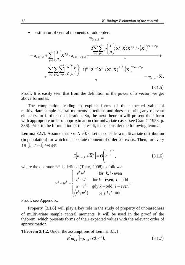
Proof: It is easily seen that from the definition of the power of a vector, we get
above formulas.
The computation leading to explicit forms of the expected value of
multivariate sample central moments is tedious and does not bring any relevant
elements for further consideration. So, the next theorem will present their form
with appropriate order of approximation (for univariate case - see Cramér 1958, p.
336). Prior to the formulation of this result, let us consider the following lemma.
Lemma 3.1.1. Assume that 0\Nr . Let us consider a multivariate distribution
(in population) for which the absolute moment of order r2 exists. Then, for every
1,...1 rt we get
2
,
t
tktr nOaE X , 6.1.3
where the operator "" is defined (Tatar, 2008) as follows:
odd - ,gdy ,
even odd, gdy
odd even, for
even - ,for
lkwv
lkvw
lkwv
lkwv
wv
lk
kl
lk
lk
lk .
Proof: see Appendix.
Property 6.1.3 will play a key role in the study of property of unbiasedness
of multivariate sample central moments. It will be used in the proof of the
theorem, which presents forms of their expected values with the relevant order of
approximation.
Theorem 3.1.2. Under the assumptions of Lemma 3.1.1.
1,,
nOmE krkr . 7.1.3

STATISTICS IN TRANSITION new series, March 2017
13
Proof: First, let us consider multivariate sample central moments of even orders.
Towards 4.1.3 we get:
XX ,2 ,12
1
2
,22,2,2 ks
s
p
p
kpsksks asEaEp
saEmE
s
p
pkpsaE
p
sp
2
12,122 ,2 X
n
El
p
p
sn
i
s
p
lpilpsi
p
l
lplp
1 2
222
0
,21 XXXX
. 8.1.3
By the assumption 0,1 mk , an easy computation shows that
n
aEks
ks
,2
,12 ,
X , 9.1.3
n
aEks
ks
,12
,2
X . 10.1.3
Note that for each ni ,...,1 and Nt we obtain the following property
2,
tt
i nOE XX . 11.1.3
Indeed, due to Minkowski's inequality in the tL1 , Schwarz's inequality in
21L and property 2.1.3 , applied to the coordinates of univariate sample mean
(Cramér, 1958, p. 332), we get:
t
k
j
tt
jij
t
ttk
j
jij
ti XXEXXEE
1
1
1
1
,XX
t
k
j
t
t
tij
t
k
j
tt
j
tij
n
AXEXEXE
1
1
2
1
2
1
1
2
122
1
2
21
2
11
2
t
t
k
j
ttij
n
CnAXE
,
for each 0nn where 0, CA .
14 K. Budny: Estimation of the central …
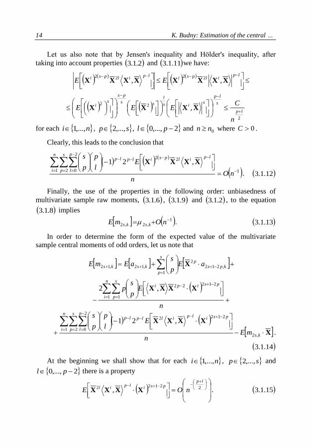
Let us also note that by Jensen's inequality and Hölder's inequality, after
taking into account properties 2.1.3 and 11.1.3 we have:
lpilpsi
lpilpsi EE XXXXXXXX ,, 2222
2
22,
lp
s
lp
sis
l
ss
ps
si
n
CEEE
XXXX
for each ni ,...,1 , sp ,...,2 , 2,...,0 pl and 0nn where 0C .
Clearly, this leads to the conclusion that
11 2
222
0
,21
nOn
El
p
p
sn
i
s
p
lpilpsi
p
l
lplpXXXX
. 12.1.3
Finally, the use of the properties in the following order: unbiasedness of
multivariate sample raw moments, 6.1.3 , 9.1.3 and 2.1.3 , to the equation
8.1.3 implies
1,2,2
nOmE ksks . 13.1.3
In order to determine the form of the expected value of the multivariate
sample central moments of odd orders, let us note that
s
p
kpsp
ksks aEp
saEmE
1
,2122
,12,12 X
n
Ep
sp
n
i
s
p
psipi
1 1
21222,2 XXXX
X
XXXX
ks
n
i
s
p
p
l
psilp
illplp
mEn
El
p
p
s
,2
1 2
2
0
2122 ,21
.
14.1.3
At the beginning we shall show that for each ni ,...,1 , sp ,...,2 and
2,...,0 pl there is a property
22122 ,
lppsi
lpil nOE XXXX . 15.1.3

STATISTICS IN TRANSITION new series, March 2017
15
Indeed, Jensen's and Hölder's inequalities, the properties 2.1.3 and 11.1.3
imply
psi
lpilpsi
lpil EE
42424
22122 ,, XXXXXXXX
12
212
,2224
1212212
2
122 , lps
ps
klps
lps
lp
lpsilps
l
lpsEE XXX
lp
lps
lp
lps
lps
l
lpslps
ps
klpsn
C
n
A
n
A
12
12
212
2
12
112
212
,2224 ,
for each 0nn where 0,, 21 CAA , which obviously is equivalent to 15.1.3 .
This implies, therefore, a property
11 2
2
0
2122 ,21
nOn
El
p
p
sn
i
s
p
p
l
psilp
illplpXXXX
.
16.1.3
Note that the reasoning analogous to the one carried out above leads to
another property expressed as
2
121222,
ppsipi nOE XXXX , 17.1.3
for each ni ,...,1 and sp ,...,1 .
Furthermore, the elementary computation establishes the equality
n
Enssii ,1212
,
XXX , 18.1.3
for every ni ,...,1 .
Owing to the conditions 17.1.3 and .18.1.3 we get the property
11 1
21222,
nOn
Ep
sp
n
i
s
p
psipiXXXX
. 19.1.3

16 K. Budny: Estimation of the central …
The proof of the theorem will be completed by determining the order of
approximation of a quantity XksmE ,2 , that takes the form
n
El
p
p
s
aEmE
n
i
s
p
llp
ipsip
l
lplp
ksks
1 1
122
0
,2,2
,21 XXXX
XX
Reasoning analogous to that shown in the proof of the property 15.1.3
justifies the expression
2
1
122,
lp
llp
ipsi nOE XXXX 20.1.3
for each ni ,...,1 , sp ,...,1 and pl ,...,0 . Thus, we get the condition
11 1
122
0
,21
nOn
El
p
p
sn
i
s
p
llp
ipsip
l
lplpXXXX
,
which, together with 10.1.3 leads to the property
1,2
nOmE ks X 21.1.3
Finally, after the consecutive application of unbiasedness of multivariate
sample raw moments and the forms 6.1.3 , 19.1.3 , 16.1.3 and 21.1.3 to the
equation 14.1.3 we get
1,12,12
nOmE ksks , 22.1.3
which completes the proof of the theorem.
Corollary 3.1.1 Multivariate sample central moments are asymptotically unbiased
estimators of the central moments of a random vector.
3.2. Consistency of the multivariate sample central moments
Our considerations in this section will focus on finding orders of
approximations of mean squared errors of multivariate sample central moments,
i.e. quantities of the form 2
,, krkrmE .

STATISTICS IN TRANSITION new series, March 2017
17
At the beginning we will take into account even-order sample central
moments. Let us note that the expression 2
,2,2 ksksmE from the formula
4.1.3 can be presented in the following form:
2
,2,2
2
,2,2 ksksksks aEmE
n
aEl
p
p
sn
i
s
p
lpilpsi
ksks
p
l
lplp
1 1
22
,2,2
0
,21 XXXX
n
l
p
p
sE
n
ii
s
pp
p
l
p
l z
lpilpsilp
z
z
z
zzzz
zzzz
1, 1, 0 0
2
1
22
21 21
1
1
2
2
,2 XXXX
.
1.2.3
Based on the property 2.1.3 , we have
12
,2,2 nOaE ksks . 2.2.3
Let us also note that
2
1
22
,2,2 ,
lplp
ilpsiksks nOaE XXXX , 3.2.3
for each ni ,...,1 , sp ,...,1 , pl ,...,0 .
In fact, considering Schwarz's inequality and Hölder's inequality we get
lp
ilpsiksksaE XXXX ,22
,2,22
lp
ipsilksks
zEaE2442
,2,2 , XXXX
d
lp
did
ps
did
ld
ksks EEEaE
2
2
22
22
,2,2 ,XXXX ,
where lpsd 2 .
Owing to the properties 2.1.3 , 11.1.3 and the condition 0,1 km , we
get
lp
ilpsiksksaE XXXX ,22
,2,22
lp
d
lp
dd
ps
kd
d
l
d n
C
n
A
n
A
n
A
1
32
,2
2
21 ,

18 K. Budny: Estimation of the central …
where 0,,, 321 CAAA , which justifies 3.2.3 .
Property 3.2.3 leads to condition
11 1
22
,2,2
0
,21
nOn
aEl
p
p
sn
i
s
p
lpilpsi
ksks
p
l
lplpXXXX
.
4.2.3
Reasoning analogous to that shown above justifies the expression
2
2
1
222121
,
llpp
z
lpilpsi
nOEzz
zzz
z XXXX , 5.2.3
for each nii ,...,1, 21 , spp ,...,1, 21 , 11 ,...,0 pl , 22 ,...,0 pl .
Therefore,
11, 1, 0 0
2
1
22
21 21
1
1
2
2
,2
nOn
l
p
p
sE
n
ii
s
pp
p
l
p
l z
lpilpsilp
z
z
z
zzzz
zzzz XXXX
.
6.2.3
Taking into account the form 1.2.3 and the properties 2.2.3 , 4.2.3 and
6.2.3 we get
12
,2,2
nOmE ksks . 7.2.3
Now, we will take into consideration the estimators of central moments of odd
order. Let us note that on the basis of 5.1.3 , the expression 2,12,12 ksksm
can be presented as the relevant linear combination of the components of the form
2,12,12 ksksa ,
122,12,12 ,,
psi
lpil
ksksa XXXX ,
122
,12,12 ,,
llp
ipsiksksa XXXX ,
122122 222
22
21
111
11 ,,,
l
lpipsipsi
lpil
XXXXXXXX .
Moving on to determine the order of approximation of the expected values of
these components, we note that 2.1.3 implies

STATISTICS IN TRANSITION new series, March 2017
19
12
,12,12
nOaE ksks . 8.2.3
2
,12,12
2
,12,12 ksksksks aEaE .
Carrying out further analysis we, in turn, apply Jensen's, Schwarz's and
Hölder's inequalities and, thanks to them, we obtain
2122
,12,12 ,,psi
lpil
ksksaE XXXX
24242
,12,12 ,psi
lpil
ksksaE XXXX
d
ps
did
lp
did
ld
dd
ksks EEEaE
12
222
21
2
,12,12 ,
XXXX ,
where lpsd 22 .
This estimation, after taking into account the properties 2.1.3 , .11.1.3 and
the fact that 0,1 km leads to
2122
,12,12 ,,psi
lpil
ksksaE XXXX
lpd
ps
kd
d
lp
d
d
l
d
d
d n
C
n
A
n
A
n
A
1
12
,23
2
2
1
1 ,
which is equivalent to the property
2
1122
,12,12 ,,
lppsi
lpil
ksks nOaE XXXX ,
for each ni ,...,1 , sp ,...,1 , pl ,...,0 .
A slight change in the proof above shows that
2
2
122
,12,12 ,,
lp
llp
ipsiksks nOaE XXXX ,
for each ni ,...,1 , sp ,...,1 , pl ,...,0 and
20 K. Budny: Estimation of the central …
2
2
1221222121
222
22
21
111
11 ,,,
llpp
llp
ipsipsilp
ilnOE XXXXXXXX
for each nii ,...,1, 21 , spp ,...,1, 21 , 11 ,...,0 pl , 22 ,...,0 pl .
The above properties leads, thus, to
12
,12,12
nOmE ksks . 9.2.3
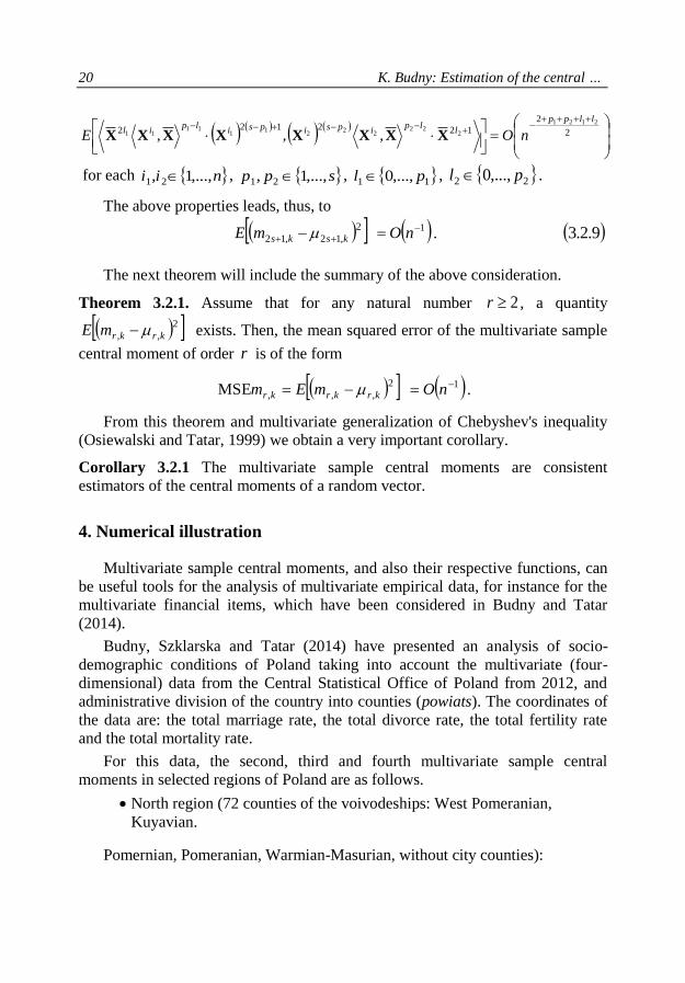
The next theorem will include the summary of the above consideration.
Theorem 3.2.1. Assume that for any natural number 2r , a quantity
2
,, krkrmE exists. Then, the mean squared error of the multivariate sample
central moment of order r is of the form
12
,,,MSE nOmEm krkrkr .
From this theorem and multivariate generalization of Chebyshev's inequality
(Osiewalski and Tatar, 1999) we obtain a very important corollary.
Corollary 3.2.1 The multivariate sample central moments are consistent
estimators of the central moments of a random vector.
4. Numerical illustration
Multivariate sample central moments, and also their respective functions, can
be useful tools for the analysis of multivariate empirical data, for instance for the
multivariate financial items, which have been considered in Budny and Tatar
(2014).
Budny, Szklarska and Tatar (2014) have presented an analysis of socio-
demographic conditions of Poland taking into account the multivariate (four-
dimensional) data from the Central Statistical Office of Poland from 2012, and
administrative division of the country into counties (powiats). The coordinates of
the data are: the total marriage rate, the total divorce rate, the total fertility rate
and the total mortality rate.
For this data, the second, third and fourth multivariate sample central
moments in selected regions of Poland are as follows.
North region (72 counties of the voivodeships: West Pomeranian,
Kuyavian.
Pomernian, Pomeranian, Warmian-Masurian, without city counties):

STATISTICS IN TRANSITION new series, March 2017
21
4744,1,2 km ,
36230
01710
12270
00220
,3
.-
.
.-
.-
m k , 5.3820,4 km .
East region (74 counties of the voivodeships: Podlaskie, Lublin,
Subcarpathian.
Lesser Poland, without city counties):
2.8700,2 km ,
34623
05310
29430
32860
,3
.
.-
.
.-
m k , 27.7891,4 km .
West region (97 counties of the voivodeships: Greater Poland, Lubusz,
Lower.
Silesian, Silesian, Opole, without city counties):
1.8058,2 km ,
1.1132
0.0448-
0.1702
0.2345-
,3 km , 9.1024,4 km .
Central region (71 counties of the voivodeships: Masovian,
Świętokrzyskie, Łódź, without city counties):
2.3571,2 km ,
1.4188-
0.0188
0.1529
0.3748-
,3 km , 14.0671,4 km .
City counties (65 counties):
2.9811,2 km ,
0.69907
0.00003
0.0828-
0.0125-
,3 km , 22.4378,4 km .
Dispersion of the distribution of the vector of the socio-demographic situation of Poland is measured by the central moments of the even orders. Note that the highest dispersion of test vector was observed in city counties while the smallest in the counties of the northern region (see Budny, Szklarska, Tatar, 2014). Central moments of odd order of multivariate distribution are parameters of location.
22 K. Budny: Estimation of the central …
They can also be considered as a measure of the asymmetry (see Tatar, 2000) and as a vector measures indicate the direction of asymmetry. The above considerations can be supplemented (see Budny, Szklarska, Tatar, 2014) using the functions of the central moments of a random vector, e.g. index of skewness (Tatar 2000) and kurtosis (Budny, Tatar 2009, Budny 2009). Let us mention that the index of skewness shows the direction of asymmetry while its square informs also about the size of the asymmetry.
The problem of estimation of this characteristics of multivariate distribution is
left for further study.
5. Conclusions
In this paper we have proposed consistent and asymptotically unbiased
estimators of the central moments of a random vector based on the power of a
vector. Essential characteristics such as mean vectors and mean squared errors
with the relevant orders of approximation have been established for them. The
central moments of even order are parameters of dispersion of the distribution of a
random vector. The moments of odd order characterize its location. These
quantities can be useful tools for the analysis of multivariate data.
Acknowledgement
Publication was financed from the funds granted to the Faculty of Finance and
Law at Cracow University of Economics, within the framework of the subsidy for
the maintenance of research potential.
REFERENCES
BILODEAU, M., BRENNER, D., (1999). Theory of Multivariate Statistics.
Springer-Verlag, New York.
BUDNY, K., (2009). Kurtoza wektora losowego. Prace Naukowe Uniwersytetu
Ekonomicznego we Wrocławiu. Ekonometria (26), Vol. 76, s. 44–54.
[Kurtosis of a random vector. Research Papers of Wrocław University of
Economics. Ekonometria (26), Vol. 76, pp. 44–54].
BUDNY, K., (2012). Kurtoza wektora losowego o wielowymiarowym rozkładzie
normalnym. w: S. FORLICZ (red.). Zastosowanie metod ilościowych
w finansach i ubezpieczeniach. CeDeWu, Warszawa, s. 41–54. [Kurtosis of
normally distributed random vector. in: S. FORLICZ (ed.). The application of
quantitative methods in finance and insurance. CeDeWu, Warsaw, pp. 41–54].
STATISTICS IN TRANSITION new series, March 2017
23
BUDNY, K., (2014). Estymacja momentów zwykłych wektora losowego
opartych na definicji potęgi wektora. Folia Oeconomica Cracoviensia,
Vol. 55, s. 81–96. [Estimation of the raw moments of a random vector based
on the definition of the power of a vector. Folia Oeconomica Cracoviensia,
Vol. 55, pp. 81–96].
BUDNY, K., TATAR, J., (2009). Kurtosis of a random vector – special types of
distributions. Statistics in Transiton - new series, Vol. 10, No. 3, pp. 445–456.
BUDNY, K., TATAR, J., (2014). Charakterystyki wielowymiarowych wielkości
finansowych oparte na definicji potęgi wektora. Studia Ekonomiczne. Zeszyty
Naukowe Uniwersytetu Ekonomicznego w Katowicach, Vol. 189, s. 27–39.
[Characteristics of multivariate financial items based on definition of the
power of a vector. Studia Ekonomiczne. Zeszyty Naukowe Uniwersytetu
Ekonomicznego w Katowicach, Vol. 189, pp. 27–39].
BUDNY, K., SZKLARSKA, M., TATAR, J., (2014). Wielowymiarowa analiza
sytuacji społeczno-demograficznej Polski. Studia i Materiały "Miscellanea
Oeconomicae", Rok 18, Nr 1/2014, s. 273–288. [Multivariate analysis of the
socio-demographic situation of Poland, Studia i Materiały "Miscellanea
Oeconomicae", Vol. 18, No. 1/2014, pp. 273–288].
CRÁMER, H., (1958). Metody matematyczne w statystyce. Wyd.1. PWN,
Warszawa. [Mathematical Methods of Statistics. 1st ed. PWN, Warsaw].
FUJIKOSHI, Y., ULYANOV, V. V., SHIMIZU, R., (2010). Mutivariate
Statistics: high-dimensional and large-sample approximations, John Wiley &
Sons, Inc.
HOLMQUIST, B., (1988). Moments and cumulants of the multivariate normal
distribution, Stochastic Analysis and Applications, 6, pp. 273–278.
ISSERLIS, L., (1918). On a Formula for the Product-Moment Coefficient of any
Order of a Normal Frequency Distribution in any Number of Variables,
Biometrika, Vol. 12, No. 1/2, Nov.
JAKUBOWSKI, J., SZTENCEL, R., (2004). Wstęp do rachunku
prawdopodobieństwa. Wyd. 3. Script, Warszawa. [Introduction to Probability
Theory. 3rd ed. Script, Warsaw].
JOHNSON, N. J., KOTZ, S., KEMP, A. W., (1992). Univariate discrete
distributions:, 2nd ed. John Wiley & Sons, Inc.
OSIEWALSKI, J., TATAR, J., (1999). Multivariate Chebyshev inequality based
on a new definition of moments of a random vector, Statistical Review,
Vol. 46, No. 2, pp. 257–260.
SHAO, J., (2003). Mathematical statistics, 2nd ed. Springer.
24 K. Budny: Estimation of the central …
TATAR, J., (1996). O niektórych miarach rozproszenia rozkładów
prawdopodobieństwa. Przegląd Statystyczny, Vol. 43, No. 3–4, s. 267–274.
[On certain measures of the diffusion of probability distribution. Statistical
Review, Vol. 43, No. 3–4, pp. 267–274].
TATAR, J. (1999). Moments of a random variable in a Hilbert space. Statistical
Review, Vol. 46, No. 2, pp. 261–271.
TATAR, J., (2000). Asymetria wielowymiarowych rozkładów
prawdopodobieństwa. Materiały z XXXV Konferencji Statystyków,
Ekonometryków i Matematyków Akademii Ekonomicznych Polski
Południowej. [Asymmetry of multivariate probability distributions.
Conference Proceedings, Cracow University of Economics].
TATAR, J., (2002). Nierówność Lapunowa dla wielowymiarowych rozkładów
prawdopodobieństwa. Zeszyty Naukowe Uniwersytetu Ekonomicznego
w Krakowie, Vol. 549, s. 5–10. [Lapunav's inequality for multivariate
probability distribution. Cracow Review of Economics and Management,
Vol. 549, pp.5–10].
TATAR, J., (2008). Miary zależności wektorów losowych o różnych wymiarach.
Zeszyty Naukowe Uniwersytetu Ekonomicznego w Krakowie, Vol. 780,
s. 53–60 [Measures of dependence of random vectors of different sizes.
Cracow Review of Economics and Management, Vol. 780, pp. 53–60].

STATISTICS IN TRANSITION new series, March 2017
25
APPENDIX
Proof of lemma 3.11.: The property 6.1.3 will be proved by considering the
cases of even and odd powers of random vectors. Reasoning (in each case) will be
based on Schwarz's inequality considered in the relevant Hilbert's space 2
kL or
2
1L .
At the beginning, let sr 2 and 12 pt where sp ,...1 . It is, therefore,
necessary to prove the property
2
1
12,122 ,
pp
kps nOaE X , 1
For the proof we will apply Schwarz's inequality in Hilbert's space 2kL
with the inner product Y,X:Y,X 2 EkL that leads to
242,122
12,122
2 ,
p
kpsp
kps EaEaE XX .
Let us note that 12
,,22
, OaEaDaE krkrkr . Thus, taking into
account the property 2.1.3 we get
1212,122
2 , pp
kps nOaE X ,
which is equivalent to the condition 1 .
Now, we consider the even numbers sr 2 and pt 2 where 1,...1 sp
In view of this, the property
ppkps nOaE
2,22 X . 2
requires the proof.
Note that Schwarz's inequality in the space 21L of the property 2.1.3
justifies the estimations
p
pkps
pkps
n
CEaEaE
2
42,22
2,22
2 XX ,

26 K. Budny: Estimation of the central …
which obviously leads to 2 .
In turn, for odd natural numbers 12 sr and 12 pt where
1,...1 sp it is necessary to prove the property
2
1
12,22
pp
kps nOaE X . 3
For this proof, let us note that Jensen's inequality, Schwarz's inequality and
the condition 2.1.3 imply a sequence of inequalities, respectively.