Estimation of Perceived Risk and Its Effect on Property Values

Jill J. McCluskey and Gordon C. Rausser*

June 25, 1999

Abstract: A dynamic discrete time model is estimated in order to analyze the evolution ofperceived risk around a hazardous waste site and its effect on property values. Residentialproperty values are modeled as a function of housing attributes and perceived risk to health froma nearby hazardous waste site using an hedonic price framework. Perceived risk enters themodel as a state equation, which includes a media coverage variable. An aggregate measure ofperceived risk is estimated and weighted by the distance to the hazardous waste site in order toindividualize risk to each location. Using a data set that spans seventeen years of property valuesaround a hazardous waste site, the results indicate that media coverage and high prior riskperception increase current perceived risk. Increased perceived risk surrounding the hazardouswaste site, in turn, lowers property values. Implications for compensation for property valuediminution caused by environmental contamination are discussed.

JEL Classification: D80, R1.

Keywords: perceived risk, hazardous waste, media, property values.

*McCluskey: Assistant Professor, Department of Agricultural Economics, PO Box 646210, Washington StateUniversity, Pullman, WA 99164-6210; Rausser: Dean and Robert Gordon Sproul Distinguished Professor, Collegeof Natural Resources, University of California, Berkeley, CA 94720 and member, Giannini Foundation ofAgricultural Economics. The authors wish to thank without implicating Amos Golan, Michael Hanemann, RonMittelhammer, Zhihua Shen, and Eric Schuck for helpful insights and computer programming expertise. They alsowish to thank Anupama Jain for her assistance with data collection. This work was supported by an EPA-NSFgrant. Jill McCluskey gratefully acknowledges financial support she received from the Fisher Center for Real Estateand Urban Economics at U.C. Berkeley’s Haas School of Business.

1

1 Introduction

The impact of perceived risk on property values has important economic and legal implications

because polluters are often sued under nuisance law by their neighbors for losses in property

values. Compensation for property value diminution caused by perceived risk is not

straightforward because of the unobservable nature of public risk perceptions. Should firms be

held responsible for the entire amount of real property values losses caused by risk perceptions

that are inflated by the media? This topic has both distributional and efficiency implications.

Firms can be required to pay compensation when their actions created no scientific risk. In terms

of efficiency, compensation requirements for perceived risk may distort real estate markets.

There is a distinction between scientifically assessed risk and perceived risk. The public’s

beliefs about environmental risk are often very different from the experts (Jenkins-Smith and

Bassett, 1994; Lindell and Earle, 1983; McClelland et al., 1990). Studies such as McClelland et

al. (1990) suggest that the public perception of health risk in close proximity to a hazardous

waste site is higher than the assessments of experts.

There are significant public policy implications that come from evolving risk perceptions and the

distinction between scientifically assessed risk and perceived risk. The Comprehensive

Environmental Response, Compensation and Liability Act (CERCLA) required that the EPA

establish criteria to prioritize sites based on risks to health, environment, and welfare. Welfare

was interpreted to mean impacts associated with health and the environment, not economic and

2

social impacts. If risk perceptions cause real losses in property values, then a more efficient

outcome may result when perceived risk is included in the resource allocation decision.

From an empirical perspective, these issues cannot be resolved without a method for measuring

perceived risk. Accordingly, in this paper we use property value data to estimate perceived risk

as it evolves over time, including the effect of the media on risk perceptions. The estimates of

perceived risk are simultaneously used to analyze the effect of perceived risk on property values.

1.1 Literature Review

It is worthwhile to briefly consider the literature on valuing environmental amenities in order to

re-think how to estimate perceived risk. Methods for valuing environmental amenities have

traditionally been categorized as indirect and direct. Indirect methods, like the hedonic price

technique and the travel cost model, use actual consumer decisions to model consumer

preferences. Consumer decisions form revealed preferences over goods, both market and non-

market. Direct methods, such as contingent valuation, ask people what they would be willing to

pay or accept for a change in an environmental amenity. Direct methods are examples of stated

preference techniques in which individuals do not actually make any behavioral changes. Direct

methods are commonly criticized because of the hypothetical nature of the questions and the fact

that actual behavior is not observed (Cummings et al., 1986; Mitchell and Carson, 1989).

Adamowicz et al. (1994) criticizes indirect methods on the basis that the models of behavior

developed constitute a maintained hypothesis about the structure of preferences that may or may

3

not be testable. They also point out that indirect methods can suffer from collinearity among

attributes. Collinearity typically precludes the isolation of factors that affect choice.

Perceived risk has been estimated primarily with direct methods. Approaches to estimating

perceived risk include the use of surveys (Bord and O’Connor, 1992; Gegax et al, 1991; Lindell

and Earle, 1983; McClelland et al, 1990; Rogers, 1997; Slovic et al, 1991), the use of surveys

within Bayesian learning framework (Smith and Johnson, 1988; Viscusi, 1985; Viscusi, 1991;

Viscusi and O’Connor, 1984), and the use of measures of concern (Loewenstein and Mather,

1990). Gayer et al (1997) starts with an objective cancer risk measure and uses a Bayesian

learning framework to update risk. In contrast to these studies, our analysis uses an indirect

approach to estimate perceived risk. Obviously the use of property value data, rather than survey

data, is less costly to implement. Both approaches attempt to capture revealed preferences over

attributes, including perceived risk.

Other researchers have analyzed the effect of media on risk. Gayer et al’s (1997) analysis of risk

tradeoffs at Superfund sites includes a news variable, which is based on Superfund coverage in a

regional newspaper. They find that their news variable has a negative and significant effect on

property values. Johnson (1988) quantifies the disruption in the market for grain products that

resulted from media coverage of product contamination by the pesticide ethylene dibromide

(EDB). Burns et al (1990) find that extensive media coverage of an event can contribute to

heightened perception of risk and amplified impacts. In contrast to previous work, this study

uses individual transaction property value data to analyze the effect of media on estimated

perceived risk.

4

2 Model and Design of the Analysis

The price of housing and land reflects consumers’ valuations of all the characteristics that are

associated with housing, including the level of perceived health risk from living near a hazardous

waste site. The level of perceived risk can be considered to be a qualitative characteristic of a

differentiated good market. Consumers can choose the level of perceived risk through their

choice of a house. Housing prices may include discounts for locations in areas with high levels

of perceived risk. If so, the price differentials may be viewed as implicit prices for different

levels of perceived risk.

Following the standard hedonic price model, the price of housing, P, is assumed to be described

by a hedonic price function, P = P(x), where x is a vector of housing attributes. The hedonic

price of an additional unit of a particular attribute is determined as the partial derivative of the

hedonic price function with respect to that particular attribute. Each consumer chooses an

optimal bundle of housing attributes and all other goods in order to maximize utility subject to a

budget constraint. The chosen bundle will place the consumer so that his indifference curve is

tangent to the price gradient, Px. The marginal willingness to pay for a change in a housing

attribute is then equal to the coefficient of the attribute (Rosen, 1974).

In order to analyze the evolution of perceived risk and its effect on property values, we estimated

a system of two equations, which includes the following hedonic price equation:

5

(1) t

n

k i

tnkitkti

d

RxP 1

211111 εβββ α +++= ∑

=+ .

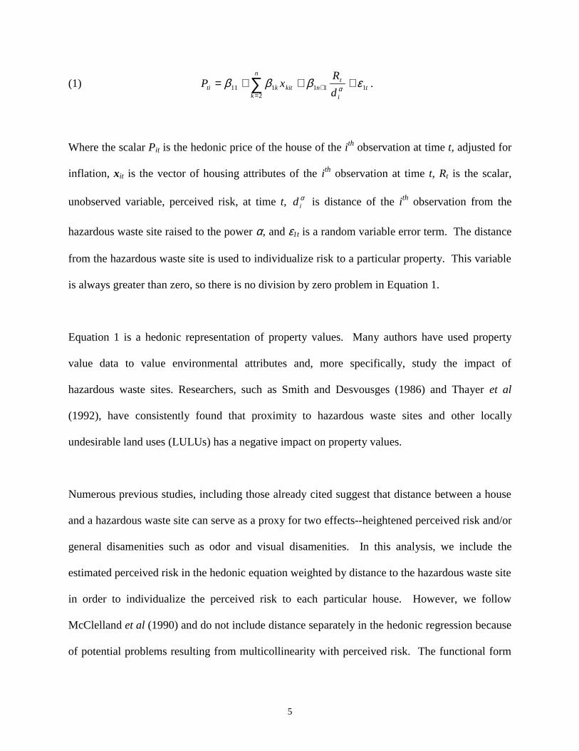
Where the scalar Pit is the hedonic price of the house of the ith observation at time t, adjusted for

inflation, xit is the vector of housing attributes of the ith observation at time t, Rt is the scalar,

unobserved variable, perceived risk, at time t, αid is distance of the ith observation from the

hazardous waste site raised to the power α, and ε1t is a random variable error term. The distance

from the hazardous waste site is used to individualize risk to a particular property. This variable

is always greater than zero, so there is no division by zero problem in Equation 1.

Equation 1 is a hedonic representation of property values. Many authors have used property

value data to value environmental attributes and, more specifically, study the impact of

hazardous waste sites. Researchers, such as Smith and Desvousges (1986) and Thayer et al

(1992), have consistently found that proximity to hazardous waste sites and other locally

undesirable land uses (LULUs) has a negative impact on property values.

Numerous previous studies, including those already cited suggest that distance between a house

and a hazardous waste site can serve as a proxy for two effects--heightened perceived risk and/or

general disamenities such as odor and visual disamenities. In this analysis, we include the

estimated perceived risk in the hedonic equation weighted by distance to the hazardous waste site

in order to individualize the perceived risk to each particular house. However, we follow

McClelland et al (1990) and do not include distance separately in the hedonic regression because

of potential problems resulting from multicollinearity with perceived risk. The functional form

6

of the distance weighting is allowed to be flexible in a limited way. The distance is raised to the

power α, which is chosen with a grid search based on minimizing the sum of squared errors.

For the hedonic price technique to result in an equilibrium of implicit markets with demand and

supply functions for each attribute, households must have full information on all housing prices

and attributes, transaction and moving costs must be zero, and the price vector must adjust

instantaneously to changes in either demand or supply (Freeman, 1993). Obviously, these

conditions are not perfectly met, and consequently, the idealized hedonic price model is not an

accurate representation of real-world real estate markets. When housing prices change so that

the marginal implicit price schedule for an attribute moves consistently in one direction,

households will consistently lag in their adjustment to that change resulting in a systematic bias.

This may be the case in our analysis of the RSR hazardous waste site, since the information

about environmental quality did change rapidly. However, as Freeman (1993) points out, it is

possible to determine the direction of the bias. Consequently, even if bias is present, the

estimates of marginal willingness to pay are still very important for applied welfare analysis

because they can be labeled as an upper bound or lower bound on the basis of that analysis.

An alternative to our chosen hedonic setup is that the causation is reversed, and homebuyers

actually use the price of homes in an area as proxies for the risks associated with proximity to the

RSR smelter site. A situation such as this could possibly be analyzed with techniques used in the

literature on prices as signals of product quality (Wolinsky, 1983). The presence of the

unobservable variable perceived risk would complicate any attempts to model the problem using

this approach.

7

To complete our model, we will add an equation describing the evolution of perceived risk. As

Smith and Johnson (1988) argue, a complete behavioral model of how people form risk

perceptions would incorporate the importance of the events at risk; the role of prior beliefs

concerning the process that generates the risk; the implications of new information about that

process; and the costs of acquiring that information.1 As with Smith and Johnson (1988), our

model is best interpreted as a reduced form approximation of the outcomes from such a

behavioral model.

Cognitive and behavioral studies, such as Slovic (1987), suggest that the formation of perceived

risk is more complicated than the traditional expected utility approach that is taken in the field of

economics. He suggests that risk appears to be influenced by two major factors: dread risk and

unknown risk. Environmental contamination is high on both counts because an individual

property owner experiences a lack of control in the remediation process, possible fatal

consequences, and the contamination is often unobservable with delayed harmful consequences.

We do not explicitly account for these factors in our model of the evolution of perceived risk.

Following a modified Bayesian learning approach, we assume that people update their prior risk

beliefs in response to new information. To complete our model, we add a state equation that

describes the evolution of perceived risk over time. Equation 2 below describes this process:

(2) tttt mediaRR 222121 εββ ++= − .

8

Where Rt-1 is lagged perceived risk, media is the weighted number of newspaper articles about

the RSR hazardous waste site, and ε2t is a random variable error term. Using generalized

maximum entropy techniques allows us to avoid making any assumptions about the distributions

of the two error terms, ε1t and ε1t; and specifically, they are not required to have identical

distributions.

Perceived risk is unobservable and changes over time. Current posterior beliefs about risk are a

function of prior beliefs about risk and current information obtained from the media. In Equation

2, people update their perception of risk with the information they receive from the media. If the

media affects the public perception of risk, then media coverage of environmental damage

should be a significant factor in determining property values.

Koné and Mullet (1994) find that the media is the dominant force in determining public risk

perception. Media coverage can affect risk perception through its informational content. It can

also affect risk perceptions through changing the salience of a particular risk to an individual.

Wildavsky (1995) argues that people usually first encounter claims of chemical harm to health

and the environment from the media. Slovic et al (1991) discuss a process labeled “social

amplification of risk.” The media is one of the major mechanisms for this process. Flynn et al

(1998) write, "News coverage of an event…may produce stigma impact by (1) initiating

awareness of a danger, (2) increasing perceptions of a known danger, (3) stimulating recall for

people with latent negative reactions that have atrophied with time, and (4) increasing the

number and geographical locations of people with knowledge of the danger."2

9

Potential homebuyers come from both within and outside the area studied. Although there was

locally intense media coverage of the RSR hazardous waste site, a concern is whether this

coverage affects the perceived risk of buyers from outside the area. The outside buyer’s

awareness of the extent and content of past media coverage of environmental contamination is

likely to be high because the vast majority of buyers use realtors.3 For a realtor that is

representing a buyer, it is his or her job to be aware and inform the client of market conditions

and factors, such as media coverage of a hazardous waste site, that may affect the market for a

particular property.

In this study the problem is, given the observable variables (price, housing attributes, the

distance to the smelter, and the media variable) to estimate the unobserved variable (perceived

risk) and the model parameters. As with Golan, Judge, and Karp (1996), we apply generalized

maximum entropy techniques to recover unknown parameters and an unobservable state

variable. Golan, Judge, and Karp (1996) offer the problem of “counting the fish in the sea.”

They estimate a system of equations in which the dependent variable in their observable equation

is fish harvest, which is a function of fishing inputs and the unobservable fish biomass in the sea.

The system is completed with a state equation that describes the evolution of the fish biomass,

which like perceived risk is an unobservable variable.

An alternative approach for a problem such as this is using Kalman filter-maximum likelihood

methodology. Burmeister et al. (1986) use a Kalman filter to estimate unobserved expected

monthly inflation. Other procedures to recover the unknown parameters in Equations (1) and (2)

exist, but they all are based on a large set of assumptions that are necessary to convert an ill-

10

posed inverse problem into a well-posed one. For example, Chow (1981) suggests a two-stage

least squares method to estimate the parameters of the state equation and feedback rule from a

linear-quadratic inverse control problem. He uses a set of equations that defines the parameters

of the optimal control rule to recover those parameters while imposing a large set of zero

restrictions.

3. Data

The data set used to quantify Equations (1) and (2) includes variables describing price and

attributes of single-family, detached homes sold within three miles of the hazardous waste site

over the period 1979 to 1995 in Dallas County, Texas.4 In order to make this dynamic

estimation problem computationally feasible, a random sample, which was limited to forty

observations per year for each of the seventeen years for a total of 680 observations. Each

observation includes information about the sale price5 of the homes and different variables which

affect the sale price, including house attributes and proximity to the RSR lead smelter.6 The

square footage of living space, number of bathrooms, and lot size describe housing quality.

The data set in this analysis includes a media variable, which was created from a random sample

of two issues per month of the Dallas Morning News in the years 1979-1995 for a total of 408

issues sampled.7 In this analysis, newspaper coverage serves as a proxy for media coverage. We

acknowledge that in recent decades television coverage as a source of news has grown in

importance relative to newspaper coverage. However, we justify our use of newspaper coverage

because its content tends to be correlated with television coverage. A variable representing

11

television coverage would be extremely difficult to obtain. In the period before EPA

identification of the RSR site, there was no newspaper coverage in the sample. The bulk of the

coverage occurred in the period in which identification of the site and cleanup occurred (1981-

1986).

As Johnson (1988) points out, the impact of the media coverage depends on how prominently it

is displayed. Johnson uses column inches of coverage to account for the differing impact of

articles. Gayer et al (1997) uses the number of words on coverage to account for different

impacts. In this analysis, we constructed a media variable by weighting each article by the

inverse of the page number of the start of the article. The number of article plus the weighted

sum of articles during a given year is the media variable for that year. Mathematically, the

media variable for year t is can then be expressed as the following

(3) ( )∑ +=i

t articlemediainumberpage

1i 1

where articlei is any article about the RSR hazardous waste site found in the sample issues in

year t, and page numberi refers to the page number at the start of articlei. These three methods of

weighting articles should be correlated. Front-page articles tend to be longer, while shorter

articles are often buried in the back of the newspaper.

A potential criticism of this media variable is that stories that provide positive information on the

site are forced to affect the price of homes in the same way as stories that provide negative

information. A justification for this is that any publicity about a hazardous waste site and a

12

limited residential area strengthens the identification that people make between that particular

residential area and environmental contamination. Using this argument, any publicity is bad

publicity. It only reminds the public about the contamination or the history of contamination.

There are examples of property values actually falling after a hazardous waste site has been

remediated. (For example, see DeSario v. Industrial Excess Landfill, Inc.8) In this perverse

scenario, if there is excessive publicity surrounding the cleanup, property values may decline.

The RSR lead smelter site is located within the geographic area contained in this data set. The

RSR lead smelter can be found in the central portion of Dallas County, approximately six miles

west of the central business district of Dallas. The smelter operated from 1934 to 1984 and was

purchased in 1971 by the RSR Corporation. The smelter emitted airborne lead, which

contaminated the soil in the surrounding areas. Lead debris created by the smelter was used in

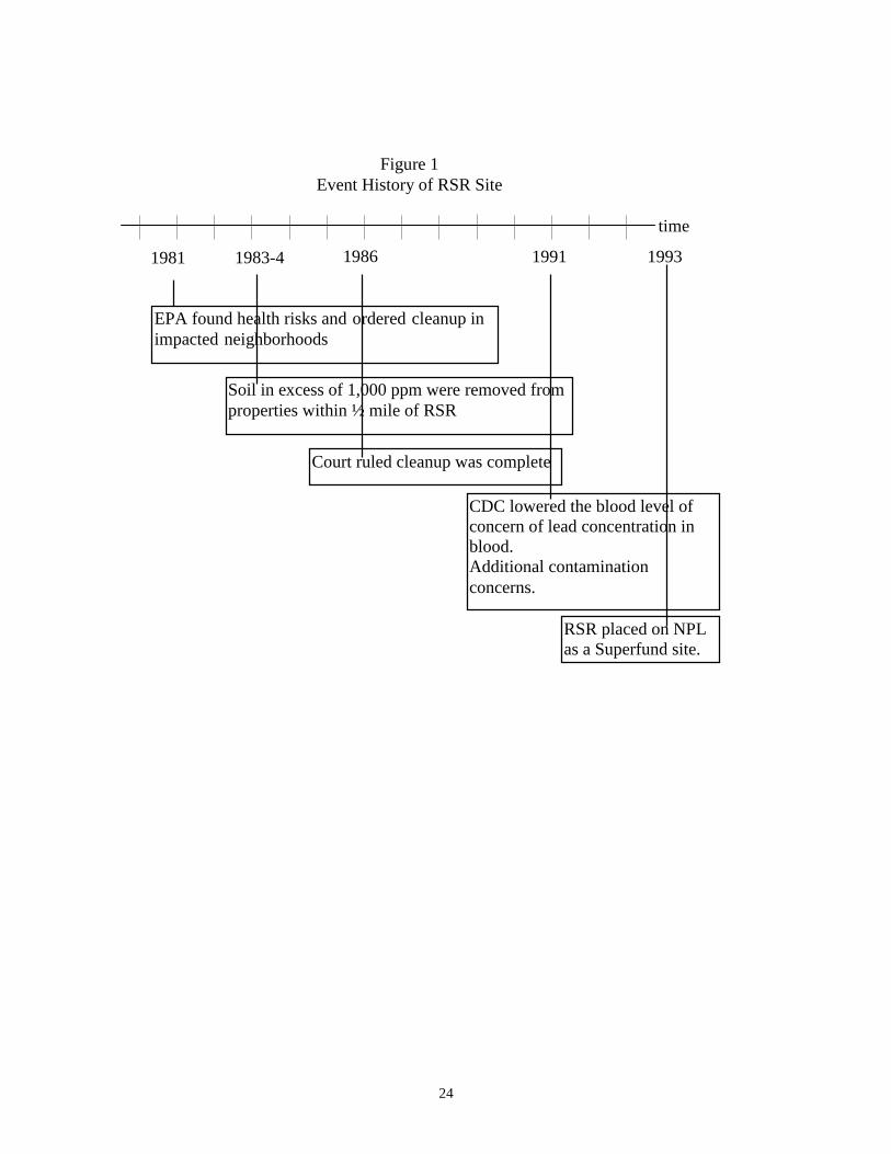
the yards and driveways of some West Dallas residences. In 1981, the EPA found health risks,

and RSR agreed to remove any contaminated soil in the neighborhoods surrounding the RSR site

using standards that were considered protective of human health at the time. In 1983 and 1984,

additional controls were imposed by the City of Dallas and the State of Texas. In 1984, the

smelter was sold to the Murmur Corporation who shut the smelter down permanently. In 1986, a

court ruled that the cleanup was complete. In the period before EPA identification of the RSR

site, there was no newspaper coverage in the sample. The bulk of the coverage occurred in the

period in which identification of the site and cleanup occurred (1981-1986). Media coverage

again increased in the period of new concern after cleanup (1991-1995).

13

In 1991, the Center for Disease Control (CDC) lowered the blood level of concern for children

from thirty to ten micrograms of lead per deciliter of blood. Low-level lead exposure in

childhood may cause reductions in intellectual capacity and attention span, reading and learning

disabilities, hyperactivity, impaired growth, or hearing loss (Kraft and Scheberle, 1995). Also in

1991, the State of Texas found hazardous waste violations at the smelter. In 1993, the RSR

smelter was placed on the Superfund National Priorities List (NPL). For a summary, see the

Event History in Figure 1.

Using a Geographic Information Systems (GIS) database, Dallas County was set up as a grid of

X and Y coordinates. Coordinates were assigned to each house and the RSR hazardous waste

site. Distance could then be calculated between any two points. A description of the variables

used in the analysis is provided in Table 1, and descriptive statistics are presented in Table 2.

Functional Form

This study follows Thayer et al (1992) and considers only the linear and semi-log (natural

logarithm of the dependent variable) functional forms for the hedonic price equation (1). A

linear specification has the obvious interpretation that a unit increase in an attribute causes the

price to rise by an amount equal to the coefficient; while with a semi-log specification, the

coefficients can be interpreted as a percent of the average house price. The following Box-Cox

transformation of the dependent variable was used on the entire data set to choose between the

linear or natural logarithmic forms for the dependent variable only.

14

(4) ( )p

P

λ λλ

λ λ

λ

=

−≠

=

10

0

,

ln ,

Using Box-Cox maximum likelihood analysis λ was estimated for each year. The yearly

estimates of λ range from -0.09 to 0.21. A value of λ = 0 implies that a semi-log specification is

best, and λ = 1 indicates a linear form is best. Confidence intervals for λ were also estimated.

The hypothesis that λ = 1 could be rejected for every year. Although the hypothesis that λ = 0

could be rejected for most years, the estimates of λ are always close to zero. Given this limited

analysis of functional form, the semi-log specification of the hedonic price equation is used in

our analysis.

Previous studies, such as McClelland, et al. (1990), have found that the impact of the waste site

on property values dissipates rapidly with distance. Therefore, the distance from the hazardous

waste site is used to individualize risk to a particular property in the hedonic price equation (2).

The functional form of the distance weighting on perceived risk depends on the value of α.

Possible values of α were selected from the set {1, 2, 3} using a grid search. We found that

setting α equal to one results in the lowest sum of squared errors from among this limited choice

set. Therefore, α is set equal to one in the estimation problem.

We also tested for serial correlation with the approach proposed by Burmeister et al. (1986). The

residuals from both the hedonic price equation (1) and the state equation for perceived risk (2)

were regressed on their lagged values up to the seventh lag. We found that the estimated

15

coefficients on all lagged residuals are insignificant at the five-percent level. One can thus

conclude that the residuals are uncorrelated with their lagged values, and that an assumed AR(1)

process describing the evolution of perceived risk is appropriate.

4 The Dynamic Estimation Problem.

The formulation in Golan, Judge, and Miller (1996) is used to convert the system of equations

(1) and (2) to a form that is consistent with the maximum entropy principle. The system of

equations in 1 and 2 is transformed so that each β1k and β2k is represented by proper probabilities

pkβ1 and pk

β2 , indexed by m, for m = 1, …, M. The support spaces for pkβ1 and pk

β2 are zkβ1 and zk

β2 ,

respectively, also indexed by m. The βik coefficients (i = 1, 2) can be expressed as

(5) ∑ ββ=m

mkmkikii zpβ , for k = 1, 2, …, τi (i = 1, 2)

The matrix βi (i = 1, 2) can then be written as

(6)

⋅

′⋅

⋅⋅⋅⋅⋅

′⋅

′

==

β

β

β

β

β

β

ββ

iK

i2

i1

ik

i2

i1

ii

p

p

p

z00

0z0

00z

pZiβ .

16

Here, iβZ is a (K x KM) matrix, and iβ

p >> 0 is a KM-dimensional vector of weights. Similarly,

εit (i = 1, 2) is represented by the discrete probabilities iεtw ,(i = 1, 2) indexed by j, for j = 1 ,…, J.

The support space for iεtw is iε

tv . The random variable error terms can then be expressed as

(7) ∑ εε=εj

tjtj vw 11it

The two sets of T unknown disturbances may be written in matrix form as

(8)

⋅

′⋅

⋅⋅⋅⋅⋅

′⋅

′

==ε

ε

ε

ε

ε

ε

ε

εε

i

i2

i1

2

1

TTw

w

w

v00

0v0

00v

wV

i

i

i

iii

where Vε

is a (T x TJ) matrices, and wε

is a TJ-dimensional vector of weights.

The support spaces for the coefficients on the explanatory variables are chosen so that they

contain all reasonable possible parameter values and are symmetric around zero. By making

these supports symmetric around zero, one is assuming that there is no prior information about

these coefficients. The support space range needs to be large enough so that the optimization

problem is feasible given the other parameters. In this estimation, the support spaces, zkβ1 and

zkβ2 , have three points (M = 3) and are an equal distance from each other. Specifically, i

kz β ´ =

( )100,0,100− , (i = 1, 2). To calculate the width of the error support space, vi, a three-standard-

17

deviations rule around zero is used. The error supports range from -3σy to 3σy, where σy is the

standard deviation of the dependent variable. In this estimation, the support spaces, vtε1 and vt

ε2 ,

have three points (J = 3) and are symmetric around zero. For example, vtε1 ´=(-3σy, 0, 3σy).

Finally, in order to simplify the statement of the GME optimization problem, the independent

variable R

dt is defined as xn+1t.

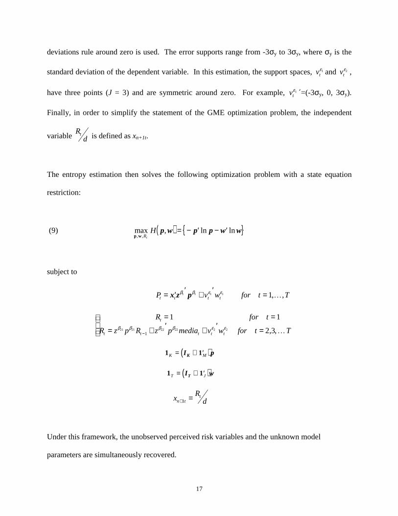
The entropy estimation then solves the following optimization problem with a state equation

restriction:

(9) ( ) { }max ln ln, ,p w Rt

H p w p p w w, = − ′ − ′

subject to

P v w for t Tt t t t= ′ ′ + ′ =x z pβ β ε ε1 1 1 1 1, ,K

R for t

R z p R z p media v w for t T

t

t t t t t

= =

= + ′ + ′ =

−

1 1

2 321 21 22 22 2 21

β β β β ε ε , ,K

( )1 1K M= ⊗ ′I pK

( )1 1T J= ⊗ ′I wT

xR

dn tt

+ =1

Under this framework, the unobserved perceived risk variables and the unknown model

parameters are simultaneously recovered.

18

5 Results

The GME estimation results of Equations 1 and 2 are presented in Table 3. All of the

explanatory variables in the hedonic price equation (Equation 1) have the expected relationship

with housing price and are statistically significant at the five-percent level. The variable of the

most interest for this study, perceived risk weighted by distance, has the expected negative

relationship with housing price. If the price vector is not adjusting rapidly to the changes in

information about environmental quality as required for an equilibrium (Freeman, 1993), then

the magnitude of coefficient on weighted perceived risk should be interpreted as an upper bound.

The explanatory variables in the state equation describing the evolution of perceived risk

(Equation 2) also have the expected relationship with perceived risk and are statistically

significant at the five-percent level. The coefficient on lagged perceived risk is positive and less

than one, which means that perceived risk is a stationary time series process. Finally, the media

coefficient is positive, which means that, as hypothesized, media coverage increases perceived

risk.

Specification of the model was evaluated by following Mittelhammer and Cardell (1997) and

analyzing the marginal values of the data constraints in the dynamic estimation problem. The

values of LaGrange multipliers on the data constraints are non-zero, which means that the data

constraints are binding. The implications are similar to rejecting an F-test to test that all the

coefficients are zero.

19

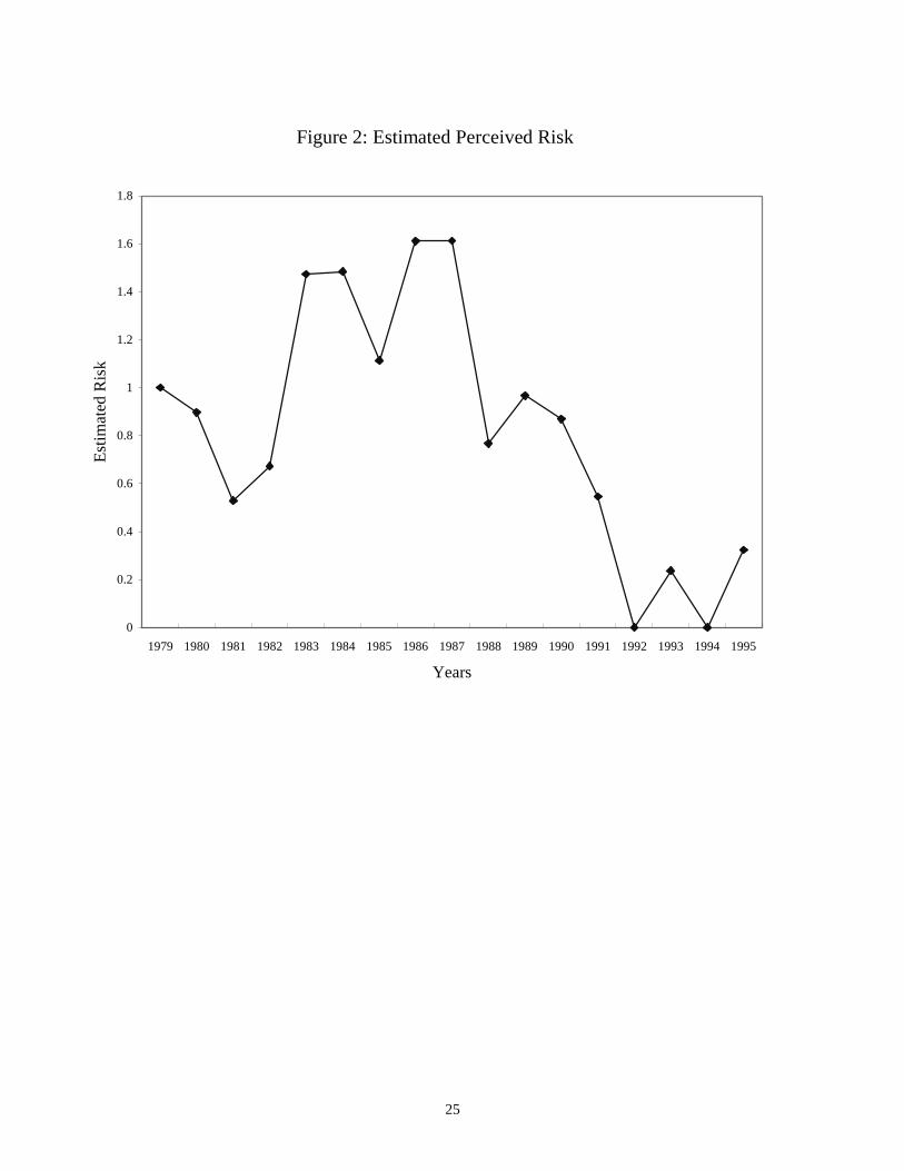
The estimates of the unobserved variable perceived risk are shown below in Figure 2. Initial

perceived risk is normalized to one. In the period before EPA identification of the RSR site,

there was no newspaper coverage in the sample. The intense media coverage that coincided with

the identification and remediation of the RSR smelter site (1981-1986) increased perceived risk,

which then decayed over time. There was a dip in perceived risk in 1985, which coincides with a

lull in media coverage. In 1985, remediation had been progressing normally for a few years, and

the RSR smelter was no longer fresh news. In 1986, when a court ruled that the cleanup was

complete, the newspaper coverage and estimated perceived risk increased. After 1987, the

estimated perceived risk falls and remains relatively low. This is despite a 1991 CDC

announcement about concern over lower levels of lead in the blood and additional concerns

about the safety of the site. One possible explanation that before identification, houses were sold

as close as 0.17 miles from the RSR site. In the period after cleanup (1987-1990), no houses

within a mile of the RSR site were sold. Therefore, in the years 1987-1990, the houses within

one mile of the smelter, which are the most affected by the smelter, no longer affect estimated

perceived risk.

Finally, in order to evaluate whether perceived risk changes over time, we tested whether the

coefficient of the lagged risk is equal to one and whether the media coefficient is equal to zero.

The generalized maximum entropy estimated coefficient less the hypothesized value divided by

the standard error of the coefficient is asymptotically distributed as a t-distribution

(Mittelhammer and Cardell, 1997). The hypotheses that the lagged perceived risk coefficient is

equal to one and that the media coefficient is equal to zero can both be rejected at the five

20

percent level. We conclude that perceived risk does evolve over time and is affected by media

coverage.

6 Conclusions

Given observable variables (price, housing attributes, distance to the hazardous waste site, and a

media coverage variable), we applied generalized maximum entropy techniques to estimate the

unknown parameters from the statistical model and an unobservable state variable, perceived

risk. Using a data set of property values around a hazardous waste site that covers the years

1979 to 1995, our results indicate that media coverage and high prior risk perceptions increase

perceived risk. Increased perceived risk surrounding the site, in turn, lowers property value.

As demonstrated above, risk perceptions change over time and can be influenced by the media.

The empirical results that perceived risk both affects property values and can be manipulated has

implications for compensation for losses in property values. With these findings, we have shown

that contaminated properties are not strategy proof. Property owners can affect outcomes with

their actions. Plaintiffs can introduce the media to contamination problems. The ensuing media

coverage in turn increases public perceived risk and lowers property values. One solution to this

dilemma is to not hold defendants responsible to pay for scientifically baseless increases in

public risk perception. The classic example of scientifically baseless perceived risk is

electromagnetic fields (EMFs) created by high voltage lines.9 Following this argument, one

should not use property value observations for compensation without adjusting for scientifically

baseless risk.

21

Scientifically assessed risk rather than perceived risk, which can be manipulated, should be the

basis of the compensation from the polluter. A compensation methodology that filters out

scientifically baseless risk by substituting scientifically assessed risk for perceived risk is ideal.

Note that the plaintiffs can still seek to recover the scientifically baseless portion of their loss in

property values. However, they must recover it from the responsible party, such as particular

media sources. An alternative approach is that the plaintiff could seek to recover the entire

amount of the property value loss from the polluter, who could in turn seek to recover the

scientifically baseless portion from the responsible parties.

In terms of efficient public policy, our findings that increased risk perceptions affect property

values, which are a real loss, could be used to argue that the EPA should consider risk

perceptions in their cost-benefit analysis for purposes of resource allocation for remediation of

contaminated sites. Ignoring perceived risk, scientists at the United States Environmental

Protection Agency (EPA) currently use dose-response relationships to calculate risk in their

decisions about how to allocate resources for remediation of environmental contamination.

Consequently, the real effect of hazardous waste sites on property values has been neglected in

cost-benefit analyses. Based on our findings, incorporating losses in property values in the

analyses could yield a different conclusion about the effectiveness of remedial actions.

Finally, McClelland et al (1990) have argued that there may be a policy role for government in

mitigating losses from the overestimation of risk in the area of environmental contamination.

Our findings that risk perceptions evolve over time and are affected by new information supports

the argument that the government could take a more active role in risk communication.

22

However, more research is needed in the area of risk communication. Lopes (1992) writes,

"[A]lthough risk experts understand that they cannot impose their views on people in a

democratic society, they do tend to define their problem as one of developing techniques for

communicating correct assessments to an inexpert public."10

23

Table 1. Variable DefinitionsVariable Description

Dprice Deflated sales price of the homeLivarea Square feet of living areaBaths Number of bathroomsLandarea Lot size in square feetDistance Miles to the RSR facilityMedia Weighted number of articles in the Dallas Morning News about

the RSR site

Table 2. Descriptive StatisticsVariable Mean Standard Deviation

Dprice 41306.18 4760.11Livarea 1496.68 641.13Baths 1.41 0.74Landarea 8932.41 4306.29Distance 2.32 0.49Media 2.33 14.04

Table 3. Perceived Risk, Generalized Maximum Entropy ResultsVariable Estimated Coefficients Standard Errors

Intercept 9.231 0.017

Living Area 5.609E-4 1.02E-5

Bathrooms 0.052 0.0107

Land Area 2.751E-5 1.68E-6

Weighted Risk -0.787 0.0316

Lagged Risk 0.785 0.105

Media 0.053 0.0244

24

EPA found health risks and ordered cleanup inimpacted neighborhoods

Soil in excess of 1,000 ppm were removed fromproperties within ½ mile of RSR

Court ruled cleanup was complete

CDC lowered the blood level ofconcern of lead concentration inblood.Additional contaminationconcerns.

RSR placed on NPLas a Superfund site.

Figure 1Event History of RSR Site

1981 1983-4 1986 1991 1993

time

25

Figure 2: Estimated Perceived Risk

0

0.2

0.4

0.6

0.8

1

1.2

1.4

1.6

1.8

1979 1980 1981 1982 1983 1984 1985 1986 1987 1988 1989 1990 1991 1992 1993 1994 1995

Years

Est

imat

ed R

isk

26

References

Adamowicz, W., J. Louviere, and M. Williams, 1994. "Combining Revealed and Stated

Preference Methods for Valuing Environmental Amenities," Journal of Environmental

Economics and Management 26: 271-92.

Bord, Richard J. and Robert E. O’Connor, 1992. “Determinants of Risk Perceptions of a

Hazardous Waste Site,” Risk Analysis 12(3): 411-416.

Burmeister, Edwin, Kent D. Wall and James T. Hamilton, 1986. "Estimation of Unobserved

Expected Monthly Inflation Using Kalman Filtering," Journal of Business & Economic

Statistics 4 (2): 147-160.

Burns, W., R. Kasperson, J. Kasperson, O. Renn, S. Emani, and P. Slovic, 1990. Social

Amplification of Risk: An Empirical Study (unpublished report available from Decision

Research, Eugene, Oregon)

Chow, G. 1981. Econometric Analysis by Control Methods (Wiley, New York, NY).

Cummings, Ronald G., D.S. Brookshire, and William D. Schulze, eds., 1986. Valuing

Environmental Goods: A State of the Arts Assessment of the Contingent Method, Rowman

and Allanheld, Totowa, NJ.

Flynn, James, Ellen Peters, C.K. Mertz, and Paul Slovic, 1998. "Risk Media and Stigma at

Rocky Flats," Risk Analysis 18: 715-727.

Freeman, A. Myrick, 1993. The Measurement of Environmental and Resource Values: Theory

and Methods, Resources for the Future, Washington, DC.

Gayer, Ted, James T. Hamilton, and W. Kip Viscusi, 1997. “Private Values of Risk Tradeoffs at

Superfund Sites: Housing Market Evidence,” unpublished paper.

27

Gegax, Douglas, Shelby Gerking and William Schulze, 1991. “Perceived Risk and the Marginal

Value of Safety,” The Review of Economics and Statistics 73(4): 589-596.

Golan, Amos, George Judge, and Larry Karp, 1996. “A Maximum Entropy Approach To

Estimation and Inference in Dynamic Models or Counting Fish in the Sea Using Maximum

Entropy,” Journal of Economic Dynamic and Control 20:559-82.

Golan, Amos, George Judge and Douglas Miller, 1996. Maximum Entropy Econometrics, John

Wiley and Sons, New York.

Jenkins-Smith, Hank and Gilbert W. Bassett Jr., 1994. “Perceived Risk and Uncertainty of

Nuclear Waste: Differences Among Science, Business, and Environmental Group Members,”

Risk Analysis 14(5): 851-856.

Johnson, F. Reed, 1988. "Economic Costs of Misinforming About Risk: The EDB Scare and the

Media," Risk Analysis 8(2): 261-270.

Koné, Daboula and Etienne Mullet, 1994. “Societal Risk Perception and Media Coverage,” Risk

Analysis 14: 21-24.

Kraft, Michael E. and Denise Scheberle, 1995. “Environmental Justice and the Allocation of

Risk: The Case of Lead and Public Health,” (Symposium on Environmental Health Policy)

Policy Studies Journal 23(1): 113-123.

Lindell, M. and T.C. Earle, 1983. “How Close is Close Enough: Public Perceptions and the

Risks of Industrial Facilities,” Risk Analysis 3(4): 245-253.

Loewenstein, George and Jane Mather, 1990. “Dynamic Processes in Risk Perception,” Journal

of Risk and Uncertainty 3:155-175.

28

Lopes, Lola L., 1992. "Risk Perception and the Perceived Public," in The Social Response to

Environmental Risk, ed. by Daniel W. Bromley and Kathleen Segerson, Kluwer Academic

Press, Boston, MA.

McClelland, Gary H., William D. Schulze, and Brian Hurd, 1990. “The effects of risk beliefs on

Property values: A case study of a hazardous waste site,” Risk Analysis 10: 485-497.

Mitchell, R.C. and Richard T. Carson, 1989. Using Surveys to Value Public Goods: The

Contingent Valuation Method, Johns Hopkins University Press for Resources for the Future,

Baltimore, MD.

Mittelhammer, Ron C. and N. Scott Cardell, 1997. "On the Consistency and Asymptotic

Normality of the Data-Constrained GME Estimator in the GLM," unpublished paper.

Rogers, George O., 1997. “The Dynamics of Risk Perception: How Does Perceived Risk

Respond to Risk Events?” Risk Analysis 17(6): 745-57.

Slovic, P., 1987. "Perception of Risk," Science 236: 280-285.

Slovic P., M. Layman, N. Kraus, J. Flynn, J. Chalmers, and G. Gesell, 1991. “Perceived Risk,

Stigma, and Potential Economic Impacts of a High-level Nuclear Waste Repository in

Nevada,” Risk Analysis 11(4): 683-696.

Smith, V. Kerry and William H. Desvousgous, 1986. “The Value of Avoiding A LULU:

Hazardous Waste Disposal Sites,” The Review of Economics and Statistics 68: 293-299.

Smith V. Kerry and F. Reed Johnson, 1988. “How Do Risk Perceptions Respond to Information?

The Case of Radon,” The Review of Economics and Statistics 70(1): 1-8.

Thayer, Mark, Heidi Albers, and Morteza Rahmatian. 1992. “The benefits of reducing exposure

to waste disposal sites: a hedonic housing value approach.” The Journal of Real Estate

Research 7, 265-282.

29

Viscusi, W. Kip, 1991. “Age Variations in Risk Perceptions and Smoking Decisions,” The

Review of Economics and Statistics 73(4): 577-588.

Viscusi, W. Kip, 1985. “A Bayesian Perspective on Biases in Risk Perception,” Economic

Letters 17: 59-62.

Viscusi W. Kip and Charles J. O’Connor, 1984. “Adaptive Responses to Chemical Labeling:

Are Workers Bayesian Decision Makers?” American Economic Review: 942-956.

Wildavsky, Aaron, 1995. But is it True? A Citizen’s Guide to Environmental Health and Safety

Issues, Harvard University Press, Cambridge, Massachusetts.

Wolinsky, Asher, 1983. "Prices as Signals of Product Quality," Review of Economic Studies

50:647-658.

30

Endnotes

1 Smith and Johnson, (1988), p. 2.

2 Flynn et al (1998), p. 717.

3 For example, according to the National Association of Realtors, 82% of buyers used realtors in 1982.

4 Dallas County Appraisal District.

5 Prices are deflated using the shelter housing price index (1982-84=100) from the Economic Report of the President.

6 Other environmental indicators, e.g., air and water quality, do not vary by location and were not included in this study.

7 The Dallas Morning News is not indexed over the entire period of the data set (1979-1995), so the data was obtained by going

through microfiche. Consequently, only a random sample of issues was used to construct the media variable.

8 587 N.E. 2d 454 (Ohio 1991)

9 Note that high voltage lines can also lower property values because they are aesthetically unappealing.

10 Lopes (1992), p. 67.