Estimation of ordered response models with sample...
27
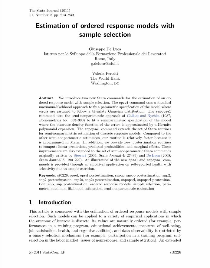
The Stata Journal (2011) 11, Number 2, pp. 213–239 Estimation of ordered response models with sample selection Giuseppe De Luca Istituto per lo Sviluppo della Formazione Professionale dei Lavoratori Rome, Italy [email protected] Valeria Perotti The World Bank Washington, DC Abstract. We introduce two new Stata commands for the estimation of an or- dered response model with sample selection. The opsel command uses a standard maximum-likelihood approach to fit a parametric specification of the model where errors are assumed to follow a bivariate Gaussian distribution. The snpopsel command uses the semi-nonparametric approach of Gallant and Nychka (1987, Econometrica 55: 363–390) to fit a semiparametric specification of the model where the bivariate density function of the errors is approximated by a Hermite polynomial expansion. The snpopsel command extends the set of Stata routines for semi-nonparametric estimation of discrete response models. Compared to the other semi-nonparametric estimators, our routine is relatively faster because it is programmed in Mata. In addition, we provide new postestimation routines to compute linear predictions, predicted probabilities, and marginal effects. These improvements are also extended to the set of semi-nonparametric Stata commands originally written by Stewart (2004, Stata Journal 4: 27–39) and De Luca (2008, Stata Journal 8: 190–220). An illustration of the new opsel and snpopsel com- mands is provided through an empirical application on self-reported health with selectivity due to sample attrition. Keywords: st0226, opsel, opsel postestimation, sneop, sneop postestimation, snp2, snp2 postestimation, snp2s, snp2s postestimation, snpopsel, snpopsel postestima- tion, snp, snp postestimation, ordered response models, sample selection, para- metric maximum-likelihood estimation, semi-nonparametric estimation 1 Introduction This article is concerned with the estimation of ordered response models with sample selection. Such models can be applied to a variety of empirical applications in which the outcome of interest is discrete, its values are naturally ordered (for example, per- formances in a training program, educational achievements, measures of well-being, job satisfaction, health, and cognitive abilities), and data observability is restricted by a binary selection mechanism (for example, participation in a training program, self- selection in the labor market, issues of nonresponse, and sample attrition). An extended c 2011 StataCorp LP st0226
Transcript of Estimation of ordered response models with sample...
The Stata Journal (2011)11, Number 2, pp. 213–239
Estimation of ordered response models withsample selection
Giuseppe De LucaIstituto per lo Sviluppo della Formazione Professionale dei Lavoratori
Rome, [email protected]
Valeria PerottiThe World BankWashington, DC
Abstract. We introduce two new Stata commands for the estimation of an or-dered response model with sample selection. The opsel command uses a standardmaximum-likelihood approach to fit a parametric specification of the model whereerrors are assumed to follow a bivariate Gaussian distribution. The snpopsel
command uses the semi-nonparametric approach of Gallant and Nychka (1987,Econometrica 55: 363–390) to fit a semiparametric specification of the modelwhere the bivariate density function of the errors is approximated by a Hermitepolynomial expansion. The snpopsel command extends the set of Stata routinesfor semi-nonparametric estimation of discrete response models. Compared to theother semi-nonparametric estimators, our routine is relatively faster because itis programmed in Mata. In addition, we provide new postestimation routinesto compute linear predictions, predicted probabilities, and marginal effects. Theseimprovements are also extended to the set of semi-nonparametric Stata commandsoriginally written by Stewart (2004, Stata Journal 4: 27–39) and De Luca (2008,Stata Journal 8: 190–220). An illustration of the new opsel and snpopsel com-mands is provided through an empirical application on self-reported health withselectivity due to sample attrition.
Keywords: st0226, opsel, opsel postestimation, sneop, sneop postestimation, snp2,snp2 postestimation, snp2s, snp2s postestimation, snpopsel, snpopsel postestima-tion, snp, snp postestimation, ordered response models, sample selection, para-metric maximum-likelihood estimation, semi-nonparametric estimation
1 Introduction
This article is concerned with the estimation of ordered response models with sampleselection. Such models can be applied to a variety of empirical applications in whichthe outcome of interest is discrete, its values are naturally ordered (for example, per-formances in a training program, educational achievements, measures of well-being,job satisfaction, health, and cognitive abilities), and data observability is restricted bya binary selection mechanism (for example, participation in a training program, self-selection in the labor market, issues of nonresponse, and sample attrition). An extended
c© 2011 StataCorp LP st0226

214 Ordered response models with sample selection
review of the model and other interesting empirical applications can be found in therecent survey on ordered response models by Greene and Hensher (2009).
After describing the structure of the basic model, we focus on consistent estimationof two alternative specifications. The parametric specification extends the classicalordered probit model by assuming that errors in the latent regression equations for theselection mechanism and the outcome variable, respectively, follow a bivariate Gaussiandistribution. Under this distributional assumption, the model parameters are estimatedby a maximum likelihood (ML) estimator, which accounts for sample selection. This isthe same estimator implemented by the ssm command of Miranda and Rabe-Hesketh(2006), a wrapper program that calls gllamm (see Rabe-Hesketh, Skrondal, and Pickles[2004]). The opsel command provided in this article is, however, much faster because itis directly programmed in the Stata ML environment. This estimator generalizes the ML
estimator of an ordered probit model provided by the official Stata command oprobit,which is known to be inconsistent if the unobservable factors affecting the outcome ofinterest are correlated with the unobservable factors affecting the selection mechanism.
Because parametric estimators of discrete choice models are known to be sensitiveto departure from distributional assumptions, we also consider a semiparametric spec-ification that avoids imposing assumptions on the distribution of the error terms. Toour knowledge, the literature on semiparametric estimation of ordered response mod-els is quite recent, and it has been mainly concerned with the estimation of standardmodels where the ordered outcome is not subject to sample selection. Semiparamet-ric estimators of a standard ordered response model have been analyzed by Lewbel(2000), Klein and Sherman (2002), Chen and Khan (2003), Stewart (2004, 2005), andCoppejans (2007).
The estimator considered in this article relies on the semi-nonparametric (SNP) ap-proach of Gallant and Nychka (1987) by generalizing the estimator of Stewart (2004).Two features of this approach are worth noticing: First, it is less computationally de-manding than other semiparametric approaches based on kernel density estimation.Second, the Monte Carlo simulations by Stewart (2005) and De Luca (2008) suggestthat SNP estimators of discrete choice models have good finite sample performancesrelative to both parametric estimators and other semiparametric estimators. The basicidea of the SNP approach is to approximate the unknown densities of the error termsby Hermite polynomial expansions and to use the resulting approximations to derivea pseudo-ML estimator for the vector of model parameters. For the model consideredin this article, SNP approximations to the unknown density and distribution functionscorrespond to the ones derived by De Luca (2008). The underlying Stata routines haveonly been improved by using Mata to speed up the estimation process. In addition, weprovide new postestimation routines to compute linear predictions, predicted probabil-ities, and marginal effects. These improvements are extended to the set of SNP Statacommands written by Stewart (2004) and De Luca (2008).
The remainder of the article is organized as follows: Section 2 introduces the sta-tistical model. The parametric ML estimator and the SNP estimator are discussed insections 3 and 4, respectively. Section 5 presents the syntax of the new and updated
G. De Luca and V. Perotti 215
commands. Examples of the use of the new opsel and snpopsel commands are pro-vided in section 6. Finally, in section 7, we use data from the first two waves of theSurvey of Health, Ageing, and Retirement in Europe (SHARE) to present results of anempirical application on self-reported health with selectivity due to sample attrition.
2 The statistical model
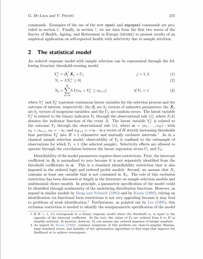
An ordered response model with sample selection can be represented through the fol-lowing bivariate threshold-crossing model
Y ∗j = β�
j Xj + Uj j = 1, 2 (1)
Y1 = I(Y ∗1 ≥ 0) (2)
Y2 =H∑
h=0
h I(αh < Y ∗2 ≤ αh+1) if Y1 = 1 (3)
where Y ∗1 and Y ∗
2 represent continuous latent variables for the selection process and theoutcome of interest, respectively; the βj are kj vectors of unknown parameters; the Xj
are kj vectors of exogenous variables; and the Uj are random errors. The latent variableY ∗
1 is related to the binary indicator Y1 through the observational rule (2), where I(A)denotes the indicator function of the event A. The latent variable Y ∗
2 is related tothe outcome Y2 through the observational rule (3), where α = (α1, . . . , αH)—withαh < αh+1, α0 = −∞, and αH+1 = +∞—is a vector of H strictly increasing thresholdsthat partition Y ∗
2 into H + 1 exhaustive and mutually exclusive intervals.1 As in aclassical sample selection model, observability of Y2 is confined to the subsample ofobservations for which Y1 = 1 (the selected sample). Selectivity effects are allowed tooperate through the correlation between the latent regression errors U1 and U2.
Identifiability of the model parameters requires three restrictions. First, the interceptcoefficient in β2 is normalized to zero because it is not separately identified from thethreshold coefficients in α. This is a standard identifiability restriction that is alsoimposed in the ordered logit and ordered probit models. Second, we assume that X1
contains at least one variable that is not contained in X2. The role of this exclusionrestriction has been discussed at length in the literature on sample selection models andmultinomial choice models. In principle, a parametric specification of the model couldbe identified through nonlinearity of the underlying distribution functions. However, asargued in similar models by Meng and Schmidt (1985) and by Keane (1992), relying onidentification via functional form restrictions is not very appealing because it may leadto problems of weak identification.2 Furthermore, as pointed out by Lee (1995), thisexclusion restriction is needed to identify the semiparametric specification of the model
1. If H = 1, (3) corresponds to a binary response model where the threshold α1 is equal to theopposite of the intercept coefficient. In the text, the values of Y2 are ordered from 0 to H tosimplify notation. In practice, however, Y2 can assume any ordered sequence of integer numbers.
2. As argued by Keane (1992), common symptoms of this problem are close-to-singular Hessian,large standard errors, and inability of the optimization algorithms to find steps that improve thelikelihood or to achieve convergence.

216 Ordered response models with sample selection
where the distribution of U1 and U2 is not assumed to be known. Third, as argued byManski (1988), identification of the semiparametric specification requires that X1 andX2 each contain at least one continuous variable. This is another standard assumptionthat guarantees that X1 and X2 have sufficiently rich supports.
The primary aim of our analysis is to obtain consistent estimates of the vector ofparameters θ2 = (β2,α) by using observations from the selected sample. Unlike aclassical sample selection model, estimators based on Heckman’s estimator cannot beapplied because of nonlinearity of the conditional mean in the second estimation step.3
In this type of model, a ML estimator remains the most attractive choice because it onlyrequires computing the contributions to the likelihood function for the H + 2 possiblerealizations of the two discrete indicators Y1 and Y2, namely (Y1 = 0), (Y1 = 1, Y2 =0), . . . , (Y1 = 1, Y2 = H). Parametric and SNP versions of this estimator are presentedin sections 3 and 4, respectively.
3 The parametric ML estimator
Our parametric specification of the model assumes that the errors U1 and U2 followa bivariate Gaussian distribution with zero means, unit variances, and correlation co-efficient ρ. This is the same distributional assumption imposed by the ssm commandof Miranda and Rabe-Hesketh (2006) when specifying a binomial family with an or-dered probit link.4 Under this parametric assumption on the distribution of the latentregression errors, the log-likelihood function for a random sample of n observations{(Y1i, Y2i,X1i,X2i) : i = 1, . . . , n} is
L(θ) =n∑
i=1
{(1 − Y1i) lnπ0i(θ) +
H∑h=0
Y1i I(Y2i = h) lnπ1hi(θ)
}(4)
where θ = (β1,β2,α, ρ) is the vector of all model parameters and (π0, π10, . . . , π1H) arethe conditional probabilities associated with the H + 2 possible realizations of Y1 andY2,5
π0(θ) = Pr (Y1 = 0) = 1 − Φ(β�1 X1) (5)
π1h(θ) = Pr (Y1 = 1, Y2 = h)
= Φ2(β�1 X1, αh+1 − β�
2 X2;−ρ) − Φ2(β�1 X1, αh − β�
2 X2;−ρ)
with Φ denoting the standardized Gaussian distribution and Φ2 denoting the bivariateGaussian distribution with zero means, unit variances, and correlation coefficient ρ.A parametric ML estimator of θ maximizes the log-likelihood function (4) over theparameter space Θ = �k1+k2+H × (−1, 1). If model (1)–(3) is correctly specified and
3. An exception is the special regressor-based approach analyzed by Dong and Lewbel (2010) in thecontext of binary choice models.
4. The parameterization of the model considered by Miranda and Rabe-Hesketh (2006) is slightlydifferent because the correlation between U1 and U2 is driven by a common random error.
5. We keep the individual subscript and the conditioning on covariates implicit to simplify notation.
G. De Luca and V. Perotti 217
the assumption on the distribution of U1 and U2 holds, then this estimator is consistentand asymptotically efficient under standard regularity conditions.
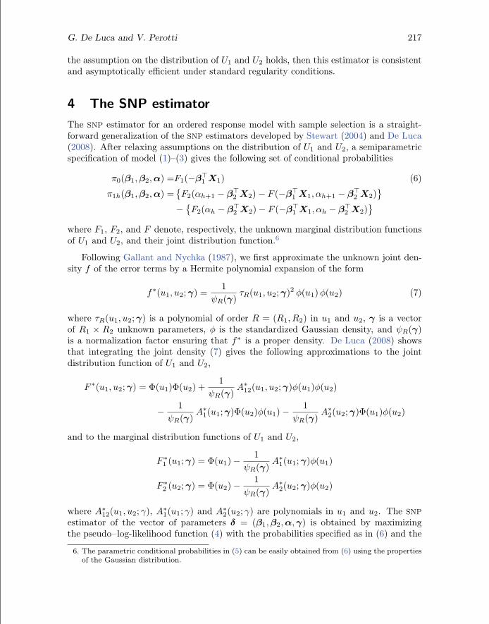
4 The SNP estimator
The SNP estimator for an ordered response model with sample selection is a straight-forward generalization of the SNP estimators developed by Stewart (2004) and De Luca(2008). After relaxing assumptions on the distribution of U1 and U2, a semiparametricspecification of model (1)–(3) gives the following set of conditional probabilities
π0(β1,β2,α) =F1(−β�1 X1) (6)
π1h(β1,β2,α) ={F2(αh+1 − β�
2 X2) − F (−β�1 X1, αh+1 − β�
2 X2)}
− {F2(αh − β�
2 X2) − F (−β�1 X1, αh − β�
2 X2)}
where F1, F2, and F denote, respectively, the unknown marginal distribution functionsof U1 and U2, and their joint distribution function.6
Following Gallant and Nychka (1987), we first approximate the unknown joint den-sity f of the error terms by a Hermite polynomial expansion of the form
f∗(u1, u2;γ) =1
ψR(γ)τR(u1, u2;γ)2 φ(u1)φ(u2) (7)
where τR(u1, u2;γ) is a polynomial of order R = (R1, R2) in u1 and u2, γ is a vectorof R1 × R2 unknown parameters, φ is the standardized Gaussian density, and ψR(γ)is a normalization factor ensuring that f∗ is a proper density. De Luca (2008) showsthat integrating the joint density (7) gives the following approximations to the jointdistribution function of U1 and U2,
F ∗(u1, u2;γ) = Φ(u1)Φ(u2) +1
ψR(γ)A∗
12(u1, u2;γ)φ(u1)φ(u2)
− 1ψR(γ)
A∗1(u1;γ)Φ(u2)φ(u1) − 1
ψR(γ)A∗
2(u2;γ)Φ(u1)φ(u2)
and to the marginal distribution functions of U1 and U2,
F ∗1 (u1;γ) = Φ(u1) − 1
ψR(γ)A∗
1(u1;γ)φ(u1)
F ∗2 (u2;γ) = Φ(u2) − 1
ψR(γ)A∗
2(u2;γ)φ(u2)
where A∗12(u1, u2; γ), A∗
1(u1; γ) and A∗2(u2; γ) are polynomials in u1 and u2. The SNP
estimator of the vector of parameters δ = (β1,β2,α,γ) is obtained by maximizingthe pseudo–log-likelihood function (4) with the probabilities specified as in (6) and the
6. The parametric conditional probabilities in (5) can be easily obtained from (6) using the propertiesof the Gaussian distribution.

218 Ordered response models with sample selection
unknown distribution functions F , F1, and F2 replaced by their approximations F ∗,F ∗
1 , and F ∗2 . This estimator is
√n-consistent, provided that R1 and R2 both increase
with sample size. Because results on the asymptotic distribution of the SNP estimatorare not available, inference is typically conducted using a parametric ML approach bytreating the order R as known. Thus, the SNP model is better viewed as a flexibleparametric specification for a fixed value of R, with the choice of R as part of themodel selection procedure. For a given sample size, the value of R may be selectedeither through a sequence of likelihood-ratio tests or by model selection criteria suchas Akaike’s information criterion and Bayesian information criterion (BIC), or by thecross-validation strategies in Coppejans and Gallant (2002).
Three remarks on the SNP estimator are worth making: First, two location restric-tions are needed because the polynomial expansion in (7) does not guarantee that U1
and U2 have zero means. As a consequence, we normalize the intercept in β1 and thefirst threshold in α to their parametric ML estimates. Second, the estimated coeffi-cients from the parametric and the SNP models are not directly comparable because inthe former, the variances of U1 and U2 are normalized to one, while in the latter theyare unconstrained functions of the Hermite polynomial parameters γ. As suggested byStewart (2004) and De Luca (2008), these scale differences can be taken into accountby comparing ratios of estimated coefficients. Alternatively, one can compare predictedprobabilities and marginal effects, which are not affected by scale differences. Third,we notice that the SNP estimator analyzed in this article is more computationally de-manding than the SNP estimator for a bivariate binary response model because theapproximations to F and F2 must be evaluated at H different points, rather than ata single point. To speed up the estimation process, we use a Mata version of the SNP
routines written by De Luca (2008). For this model, the Mata routine is between fourand six times faster than the standard Stata routine.7
5 Stata commands
The new Stata commands opsel and snpopsel provide, respectively, the parametric ML
estimator and the SNP estimator of an ordered response model with sample selection.The general syntax of these commands is as follows:
opsel equation1[if
] [in
] [weight
], select(equation2,
[noconstant
offset(varname)])
[offset(varname) robust from(matname) level(#)
maximize options]
snpopsel equation1[if
] [in
] [weight
], select(equation2,
[noconstant
offset(varname)])
[offset(varname) order1(#) order2(#)
dplot(filename) from(matname) level(#) robust maximize options]
7. Estimation time usually increases with the number of observations, the number of categories of theordered outcome Y2, and the order R = (R1, R2) of the Hermite polynomial expansion.

G. De Luca and V. Perotti 219
where equation1 is specified as8
depvar varlist
and equation2 is specified as
depvar s = varlist s
Both commands are written using ml model lf and share the same features of allStata estimation commands, including access to the estimation results and options forthe maximization process (see [R] maximize). version 10.1 is the earliest versionof Stata that can be used to run the routines. However, due to the new optimizationengine used by the ml command under version 11 (see [R] ml), the routines use versioncontrol to allow for use of both version 10.1 and version 11.0.9 This version controlis established on the basis of c(version) so it can be easily changed by users (see[P] version). fweight, iweight, and pweight are allowed (see [U] 11.1.6 weight).Most options are similar to those of other Stata estimation commands. A descriptionof command-specific options and the available postestimation commands is providedbelow. See the opsel and snpopsel help file for descriptions of other options.
5.1 Option of the opsel command
from(matname) specifies the name of the matrix containing the starting values. Bydefault, starting values are the probit estimates for the coefficients in the binary se-lection equation, the oprobit estimates for the coefficients in the outcome equation,and zero for the correlation coefficient.
5.2 Options of the snpopsel command
order1(#) specifies the order R1 to be used in the bivariate Hermite polynomial ex-pansion. The default is order1(3).
order2(#) specifies the order R2 to be used in the bivariate Hermite polynomial ex-pansion. The default is order2(3).
dplot(filename) plots the estimated marginal densities of the two error terms togetherwith Gaussian densities with the same estimated means and variances. This optiongenerates three new graphs: The first is a plot of the estimated marginal density ofU1 and is stored as filename 1. The second is a plot of the estimated marginal densityof U2 and is stored as filename 2. The third combines filename 1 and filename 2 ina single graph and is stored as filename.
8. In equation1, the noconstant option is specified by default.9. Our tests suggest that the ml command under version 11 has slightly better numerical stability
than the ml command under version 10.

220 Ordered response models with sample selection
from(matname) specifies the name of the matrix containing starting values. By default,starting values are the parametric ML estimates from the opsel command, plus avector of zeros for the Hermite polynomial parameters γ. If the opsel commanddoes not converge, then starting values are the probit estimates for the coefficientsin the selection equation, the oprobit estimates for the coefficients in the outcomeequation, plus a vector of zeros for the Hermite polynomial parameters γ.
5.3 Postestimation commands after opsel and snpopsel
After parametric and SNP estimation with opsel or snpopsel, the predict commandcan be used to compute linear predictions and predicted probabilities. The syntax ofthis command is
predict newvarlist[if
] [in
] [, pmargin pjoint pcond psel xb xbsel
outcome(#)]
where
pmargin calculates the predicted marginal probabilities Pr (Y2 = h). If the outcome()option is not specified, newvarlist must contain H + 1 new variables, where H is thenumber of categories of the dependent variable. If the outcome() option is specified,newvarlist must contain only one new variable. pmargin is the default.
pjoint calculates the predicted joint probabilities Pr (Y1 = 1, Y2 = h). If the outcome()option is not specified, newvarlist must containH+1 new variables. If the outcome()option is specified, newvarlist must contain only one new variable.
pcond calculates the predicted conditional probabilities Pr (Y2 = h | Y1 = 1). If theoutcome() option is not specified, newvarlist must contain H + 1 new variables,where H is the number of categories of the dependent variable. If the outcome()option is specified, newvarlist must contain only one new variable.
psel calculates the predicted selection probability Pr (Y1 = 1). In this case, newvarlistmust contain only one new variable.
xb calculates the linear prediction β �2 X2 of the outcome equation. In this case, new-
varlist must contain only one new variable.
xbsel calculates the linear prediction β �1 X1 for the selection equation, including the
contribution of the constrained intercept. In this case, newvarlist must contain onlyone new variable.
outcome(#) specifies the category of the dependent variable Y2 for which the marginal,joint, or conditional probability must be calculated.
In addition, the margins command allows the user to make an inference on any ofthe statistics that can be computed from predictions of a previously fit model at fixedvalues of the covariates (see [R] margins). The lists of covariates in equation1 and

G. De Luca and V. Perotti 221
equation2 cannot contain factor-variable operators. Thus it is the user’s responsibilityto ensure that all functionally related covariates in the model are set to the appropriatefixed values when one of them is set to a fixed value. Some examples are provided insections 6 and 7.
5.4 Updated routines of other SNP commands
Updated versions of the SNP Stata commands (sneop, snp, snp2, and snp2s) writtenby Stewart (2004) and De Luca (2008) are also provided. As discussed at length inthis article, these commands fit, respectively, a univariate ordered response model, aunivariate binary response model, a bivariate binary response model, and a bivariatebinary response model with sample selection. The updated routines account for twoimportant improvements. First, they are faster and more precise because they arewritten in Mata. Second, after SNP estimation, one can use the predict and themargins commands to compute linear predictions, predicted probabilities, and marginaleffects.10 In the following sections, we refer to the models considered by Stewart (2004)and De Luca (2008) to briefly describe the syntax of the predict commands associatedwith these SNP estimators.
The syntax of predict after sneop is
predict newvarlist[if
] [in
] [, pr xb outcome(#)
]where pr, the default, calculates the predicted probabilities Pr (Y2 = h) and xb calcu-lates the linear prediction, ignoring the contribution of the cutpoints.
The syntax of predict after snp is
predict newvar[if
] [in
] [, pr xb
]where pr, the default, calculates the predicted probability of success Pr (Y1 = 1) and xbcalculates the linear prediction, including the contribution of the constrained intercept.
The syntax of predict after snp2 is
predict newvar[if
] [in
] [, p11 p10 p01 p00 pmarg1 pmarg2 pcond1 pcond2
xb1 xb2]
where p11, the default, calculates the joint probability Pr (Y1 = 1, Y2 = 1); p10 cal-culates the joint probability Pr (Y1 = 1, Y2 = 0); p01 calculates the joint probabilityPr (Y1 = 0, Y2 = 1); p00 calculates the joint probability Pr (Y1 = 0, Y2 = 0); pmarg1 cal-culates the marginal probability Pr (Y1 = 1); pmarg2 calculates the marginal probabilityPr (Y2 = 1); pcond1 calculates the conditional probability Pr (Y1 = 1 | Y2 = 1); pcond2calculates the conditional probability Pr (Y2 = 1 | Y1 = 1); xb1 calculates the linear pre-diction of the first equation, including the contribution of the constrained intercept; and
10. The new routines also take into account other minor drawbacks of the old routines.
222 Ordered response models with sample selection
xb2 calculates the linear prediction of the second equation, including the contributionof the constrained intercept.
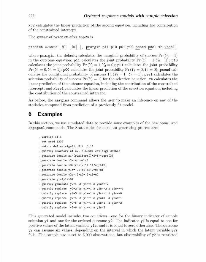
The syntax of predict after snp2s is
predict newvar[if
] [in
] [, pmargin p11 p10 p01 p00 pcond psel xb xbsel
]where pmargin, the default, calculates the marginal probability of success Pr (Y2 = 1)in the outcome equation; p11 calculates the joint probability Pr (Y1 = 1, Y2 = 1); p10calculates the joint probability Pr (Y1 = 1, Y2 = 0); p01 calculates the joint probabilityPr (Y1 = 0, Y2 = 1); p00 calculates the joint probability Pr (Y1 = 0, Y2 = 0); pcond cal-culates the conditional probability of success Pr (Y2 = 1 | Y1 = 1); psel calculates theselection probability of success Pr (Y1 = 1) for the selection equation; xb calculates thelinear prediction of the outcome equation, including the contribution of the constrainedintercept; and xbsel calculates the linear prediction of the selection equation, includingthe contribution of the constrained intercept.
As before, the margins command allows the user to make an inference on any of thestatistics computed from prediction of a previously fit model.
6 Examples
In this section, we use simulated data to provide some examples of the new opsel andsnpopsel commands. The Stata codes for our data-generating process are:
. version 11.1
. set seed 1234
. matrix define sig=(1,.3 \ .3,1)
. quietly drawnorm u1 u2, n(5000) cov(sig) double
. generate double x1=(runiform()*2-1)*sqrt(3)
. generate double x2=rnormal()
. generate double x3=(rchi2(1)-1)/sqrt(2)
. generate double y1s=-.1+x1-x2+2*x3+u1
. generate double y2s=.5*x2-.5*x3+u2
. generate y1=(y1s>0)
. quietly generate y2=1 if y1==1 & y2s<=-2
. quietly replace y2=2 if y1==1 & y2s>-2 & y2s<=-1
. quietly replace y2=3 if y1==1 & y2s>-1 & y2s<=0
. quietly replace y2=4 if y1==1 & y2s>0 & y2s<=1
. quietly replace y2=5 if y1==1 & y2s>1 & y2s<=2
. quietly replace y2=6 if y1==1 & y2s>2
This generated model includes two equations—one for the binary indicator of sampleselection y1 and one for the ordered outcome y2. The indicator y1 is equal to one forpositive values of the latent variable y1s, and it is equal to zero otherwise. The outcomey2 can assume six values, depending on the interval in which the latent variable y2sfalls. The sample size is set to 5,000 observations, but observability of y2 is restricted
G. De Luca and V. Perotti 223
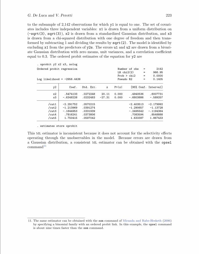
to the subsample of 2,142 observations for which y1 is equal to one. The set of covari-ates includes three independent variables: x1 is drawn from a uniform distribution on(-sqrt(3), sqrt(3)), x2 is drawn from a standardized Gaussian distribution, and x3is drawn from a chi-squared distribution with one degree of freedom and then trans-formed by subtracting 1 and dividing the results by sqrt(2). The model is identified byexcluding x1 from the predictors of y2s. The errors u1 and u2 are drawn from a bivari-ate Gaussian distribution with zero means, unit variances, and a correlation coefficientequal to 0.3. The ordered probit estimates of the equation for y2 are
. oprobit y2 x2 x3, nolog
Ordered probit regression Number of obs = 2142LR chi2(2) = 966.95Prob > chi2 = 0.0000
Log likelihood = -2956.4436 Pseudo R2 = 0.1405
y2 Coef. Std. Err. z P>|z| [95% Conf. Interval]
x2 .5474133 .0272248 20.11 0.000 .4940536 .6007731x3 -.6348228 .0232483 -27.31 0.000 -.6803886 -.589257
/cut1 -2.291752 .0570215 -2.403513 -2.179992/cut2 -1.213969 .0391274 -1.290657 -1.13728/cut3 -.1844953 .0331939 -.2495542 -.1194364/cut4 .7816241 .0373806 .7083594 .8548888/cut5 1.750415 .0597042 1.633397 1.867433
. estimates store oprobit
This ML estimator is inconsistent because it does not account for the selectivity effectsoperating through the unobservables in the model. Because errors are drawn froma Gaussian distribution, a consistent ML estimator can be obtained with the opselcommand11
11. The same estimator can be obtained with the ssm command of Miranda and Rabe-Hesketh (2006)by specifying a binomial family with an ordered probit link. In this example, the opsel commandis about nine times faster than the ssm command.
224 Ordered response models with sample selection
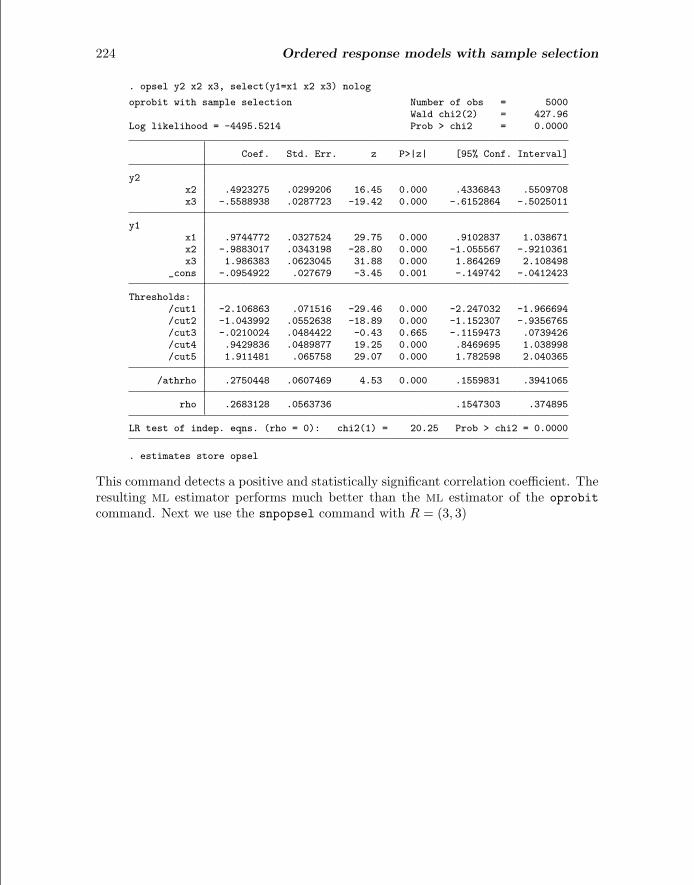
. opsel y2 x2 x3, select(y1=x1 x2 x3) nolog
oprobit with sample selection Number of obs = 5000Wald chi2(2) = 427.96
Log likelihood = -4495.5214 Prob > chi2 = 0.0000
Coef. Std. Err. z P>|z| [95% Conf. Interval]
y2x2 .4923275 .0299206 16.45 0.000 .4336843 .5509708x3 -.5588938 .0287723 -19.42 0.000 -.6152864 -.5025011
y1x1 .9744772 .0327524 29.75 0.000 .9102837 1.038671x2 -.9883017 .0343198 -28.80 0.000 -1.055567 -.9210361x3 1.986383 .0623045 31.88 0.000 1.864269 2.108498
_cons -.0954922 .027679 -3.45 0.001 -.149742 -.0412423
Thresholds:/cut1 -2.106863 .071516 -29.46 0.000 -2.247032 -1.966694/cut2 -1.043992 .0552638 -18.89 0.000 -1.152307 -.9356765/cut3 -.0210024 .0484422 -0.43 0.665 -.1159473 .0739426/cut4 .9429836 .0489877 19.25 0.000 .8469695 1.038998/cut5 1.911481 .065758 29.07 0.000 1.782598 2.040365
/athrho .2750448 .0607469 4.53 0.000 .1559831 .3941065
rho .2683128 .0563736 .1547303 .374895
LR test of indep. eqns. (rho = 0): chi2(1) = 20.25 Prob > chi2 = 0.0000
. estimates store opsel
This command detects a positive and statistically significant correlation coefficient. Theresulting ML estimator performs much better than the ML estimator of the oprobitcommand. Next we use the snpopsel command with R = (3, 3)
G. De Luca and V. Perotti 225
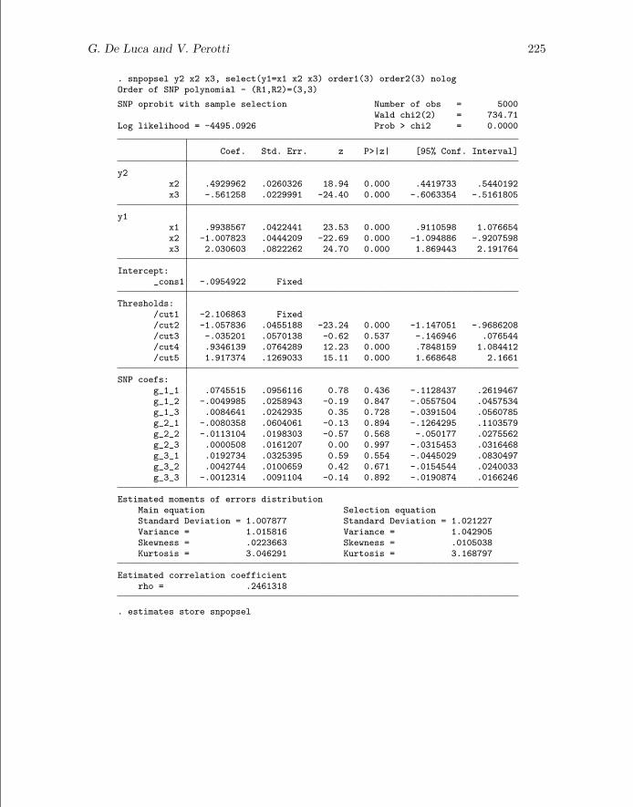
. snpopsel y2 x2 x3, select(y1=x1 x2 x3) order1(3) order2(3) nologOrder of SNP polynomial - (R1,R2)=(3,3)
SNP oprobit with sample selection Number of obs = 5000Wald chi2(2) = 734.71
Log likelihood = -4495.0926 Prob > chi2 = 0.0000
Coef. Std. Err. z P>|z| [95% Conf. Interval]
y2x2 .4929962 .0260326 18.94 0.000 .4419733 .5440192x3 -.561258 .0229991 -24.40 0.000 -.6063354 -.5161805
y1x1 .9938567 .0422441 23.53 0.000 .9110598 1.076654x2 -1.007823 .0444209 -22.69 0.000 -1.094886 -.9207598x3 2.030603 .0822262 24.70 0.000 1.869443 2.191764
Intercept:_cons1 -.0954922 Fixed
Thresholds:/cut1 -2.106863 Fixed/cut2 -1.057836 .0455188 -23.24 0.000 -1.147051 -.9686208/cut3 -.035201 .0570138 -0.62 0.537 -.146946 .076544/cut4 .9346139 .0764289 12.23 0.000 .7848159 1.084412/cut5 1.917374 .1269033 15.11 0.000 1.668648 2.1661
SNP coefs:g_1_1 .0745515 .0956116 0.78 0.436 -.1128437 .2619467g_1_2 -.0049985 .0258943 -0.19 0.847 -.0557504 .0457534g_1_3 .0084641 .0242935 0.35 0.728 -.0391504 .0560785g_2_1 -.0080358 .0604061 -0.13 0.894 -.1264295 .1103579g_2_2 -.0113104 .0198303 -0.57 0.568 -.050177 .0275562g_2_3 .0000508 .0161207 0.00 0.997 -.0315453 .0316468g_3_1 .0192734 .0325395 0.59 0.554 -.0445029 .0830497g_3_2 .0042744 .0100659 0.42 0.671 -.0154544 .0240033g_3_3 -.0012314 .0091104 -0.14 0.892 -.0190874 .0166246
Estimated moments of errors distributionMain equation Selection equationStandard Deviation = 1.007877 Standard Deviation = 1.021227Variance = 1.015816 Variance = 1.042905Skewness = .0223663 Skewness = .0105038Kurtosis = 3.046291 Kurtosis = 3.168797
Estimated correlation coefficientrho = .2461318
. estimates store snpopsel

226 Ordered response models with sample selection
Because of the large sample size, the estimated correlation coefficient and moments(standard deviation, skewness, and kurtosis) of the distributions of the error terms arequite close to the true values. The intercept coefficient in the selection equation and thefirst threshold coefficient are set equal to their parametric estimates because they canbe absorbed in the unknown distribution functions and are not separately identified.Moreover, because of the different scale normalizations, SNP estimates of the remainingcoefficients are not directly comparable with the parametric probit estimates. Below wecompare ratios of the estimated coefficients using the nlcom command:
. quietly estimates restore opsel
. nlcom (b12_b11: [y1]_b[x2]/[y1]_b[x1]) (b13_b11: [y1]_b[x3]/[y1]_b[x1])> (b23_b22: [y2]_b[x3]/[y2]_b[x2]) (cut2_b22: [cut2]_b[_cons]/[y2]_b[x2])> (cut3_b22: [cut3]_b[_cons]/[y2]_b[x2]) (cut4_b22: [cut4]_b[_cons]/[y2]_b[x2])> (cut5_b22: [cut5]_b[_cons]/[y2]_b[x2]), nohead
Coef. Std. Err. z P>|z| [95% Conf. Interval]
b12_b11 -1.014187 .0363359 -27.91 0.000 -1.085404 -.9429695b13_b11 2.038409 .065566 31.09 0.000 1.909902 2.166916b23_b22 -1.135207 .0619191 -18.33 0.000 -1.256566 -1.013848
cut2_b22 -2.120522 .1083519 -19.57 0.000 -2.332888 -1.908157cut3_b22 -.0426593 .0969984 -0.44 0.660 -.2327727 .1474541cut4_b22 1.915358 .18147 10.55 0.000 1.559684 2.271033cut5_b22 3.88254 .2947022 13.17 0.000 3.304934 4.460145
. quietly estimates restore snpopsel
. nlcom (b12_b11: [y1]_b[x2]/[y1]_b[x1]) (b13_b11: [y1]_b[x3]/[y1]_b[x1])> (b23_b22: [y2]_b[x3]/[y2]_b[x2]) (cut2_b22: [cut2]_b[_cons]/[y2]_b[x2])> (cut3_b22: [cut3]_b[_cons]/[y2]_b[x2]) (cut4_b22: [cut4]_b[_cons]/[y2]_b[x2])> (cut5_b22: [cut5]_b[_cons]/[y2]_b[x2]), nohead
Coef. Std. Err. z P>|z| [95% Conf. Interval]
b12_b11 -1.014053 .0362937 -27.94 0.000 -1.085187 -.9429183b13_b11 2.043155 .065341 31.27 0.000 1.915089 2.171221b23_b22 -1.138463 .0633154 -17.98 0.000 -1.262559 -1.014367
cut2_b22 -2.145728 .1320379 -16.25 0.000 -2.404518 -1.886939cut3_b22 -.0714022 .1151801 -0.62 0.535 -.2971509 .1543466cut4_b22 1.895783 .1858832 10.20 0.000 1.531459 2.260107cut5_b22 3.889227 .3119916 12.47 0.000 3.277735 4.50072
Once differences in the scale of the error terms are taken into account, the SNP esti-mates of the coefficients and their standard errors are very close to those obtained withthe parametric ML estimator. Of course, in this Gaussian design, the SNP estimatesare somewhat less efficient than the parametric ML estimates. An alternative way ofcomparing the estimation results is that of using the margins command to computemarginal effects. Below we compare the true and the estimated marginal effects for theprobability Pr (Y2 = 1) at the sample means of the continuous covariates x2 and x3:
G. De Luca and V. Perotti 227
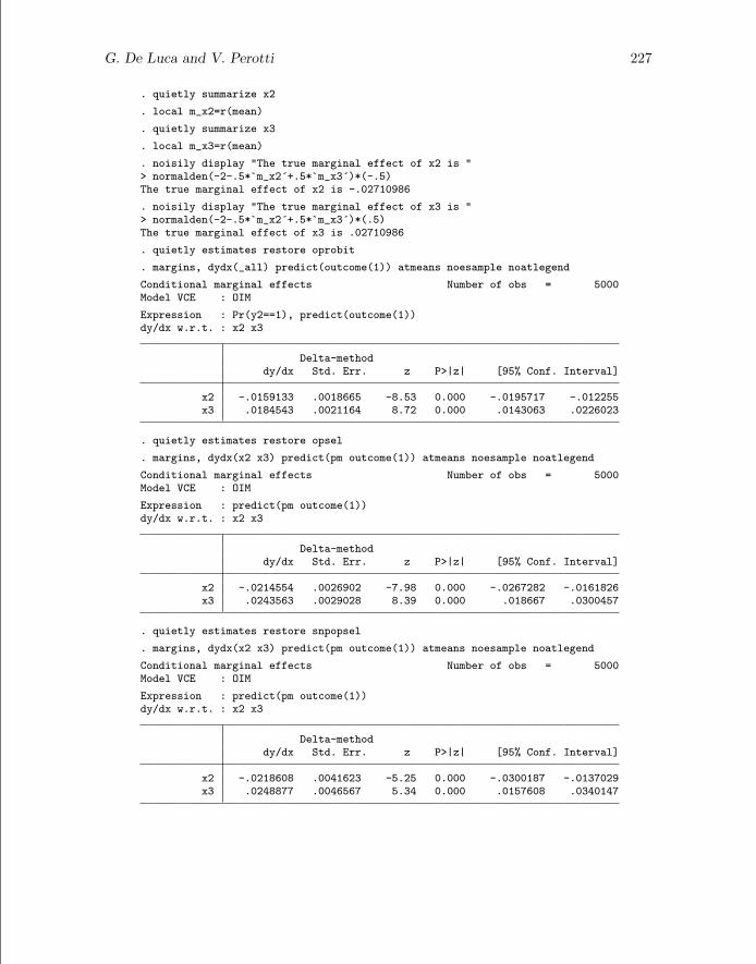
. quietly summarize x2
. local m_x2=r(mean)
. quietly summarize x3
. local m_x3=r(mean)
. noisily display "The true marginal effect of x2 is "> normalden(-2-.5*`m_x2´+.5*`m_x3´)*(-.5)The true marginal effect of x2 is -.02710986
. noisily display "The true marginal effect of x3 is "> normalden(-2-.5*`m_x2´+.5*`m_x3´)*(.5)The true marginal effect of x3 is .02710986
. quietly estimates restore oprobit
. margins, dydx(_all) predict(outcome(1)) atmeans noesample noatlegend
Conditional marginal effects Number of obs = 5000Model VCE : OIM
Expression : Pr(y2==1), predict(outcome(1))dy/dx w.r.t. : x2 x3
Delta-methoddy/dx Std. Err. z P>|z| [95% Conf. Interval]
x2 -.0159133 .0018665 -8.53 0.000 -.0195717 -.012255x3 .0184543 .0021164 8.72 0.000 .0143063 .0226023
. quietly estimates restore opsel
. margins, dydx(x2 x3) predict(pm outcome(1)) atmeans noesample noatlegend
Conditional marginal effects Number of obs = 5000Model VCE : OIM
Expression : predict(pm outcome(1))dy/dx w.r.t. : x2 x3
Delta-methoddy/dx Std. Err. z P>|z| [95% Conf. Interval]
x2 -.0214554 .0026902 -7.98 0.000 -.0267282 -.0161826x3 .0243563 .0029028 8.39 0.000 .018667 .0300457
. quietly estimates restore snpopsel
. margins, dydx(x2 x3) predict(pm outcome(1)) atmeans noesample noatlegend
Conditional marginal effects Number of obs = 5000Model VCE : OIM
Expression : predict(pm outcome(1))dy/dx w.r.t. : x2 x3
Delta-methoddy/dx Std. Err. z P>|z| [95% Conf. Interval]
x2 -.0218608 .0041623 -5.25 0.000 -.0300187 -.0137029x3 .0248877 .0046567 5.34 0.000 .0157608 .0340147
228 Ordered response models with sample selection
The marginal effects of the oprobit command are clearly underestimated, and the 95%confidence intervals do not include the true values. On the other hand, the marginaleffects of the opsel and snpopsel commands are not statistically different from thetrue values.
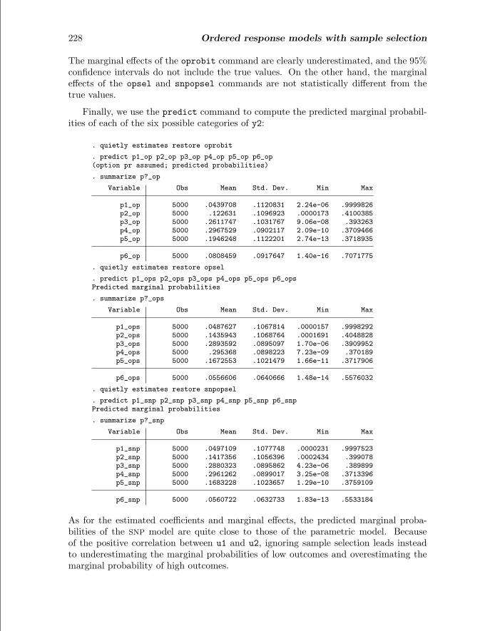
Finally, we use the predict command to compute the predicted marginal probabil-ities of each of the six possible categories of y2:
. quietly estimates restore oprobit
. predict p1_op p2_op p3_op p4_op p5_op p6_op(option pr assumed; predicted probabilities)
. summarize p?_op
Variable Obs Mean Std. Dev. Min Max
p1_op 5000 .0439708 .1120831 2.24e-06 .9999826p2_op 5000 .122631 .1096923 .0000173 .4100385p3_op 5000 .2611747 .1031767 9.06e-08 .393263p4_op 5000 .2967529 .0902117 2.09e-10 .3709466p5_op 5000 .1946248 .1122201 2.74e-13 .3718935
p6_op 5000 .0808459 .0917647 1.40e-16 .7071775
. quietly estimates restore opsel
. predict p1_ops p2_ops p3_ops p4_ops p5_ops p6_opsPredicted marginal probabilities
. summarize p?_ops
Variable Obs Mean Std. Dev. Min Max
p1_ops 5000 .0487627 .1067814 .0000157 .9998292p2_ops 5000 .1435943 .1068764 .0001691 .4048828p3_ops 5000 .2893592 .0895097 1.70e-06 .3909952p4_ops 5000 .295368 .0898223 7.23e-09 .370189p5_ops 5000 .1672553 .1021479 1.66e-11 .3717906
p6_ops 5000 .0556606 .0640666 1.48e-14 .5576032
. quietly estimates restore snpopsel
. predict p1_snp p2_snp p3_snp p4_snp p5_snp p6_snpPredicted marginal probabilities
. summarize p?_snp
Variable Obs Mean Std. Dev. Min Max
p1_snp 5000 .0497109 .1077748 .0000231 .9997523p2_snp 5000 .1417356 .1056396 .0002434 .399078p3_snp 5000 .2880323 .0895862 4.23e-06 .389899p4_snp 5000 .2961262 .0899017 3.25e-08 .3713396p5_snp 5000 .1683228 .1023657 1.29e-10 .3759109
p6_snp 5000 .0560722 .0632733 1.83e-13 .5533184
As for the estimated coefficients and marginal effects, the predicted marginal proba-bilities of the SNP model are quite close to those of the parametric model. Becauseof the positive correlation between u1 and u2, ignoring sample selection leads insteadto underestimating the marginal probabilities of low outcomes and overestimating themarginal probability of high outcomes.

G. De Luca and V. Perotti 229
7 Empirical application
In this section, we present an empirical application on self-reported health (SRH) sta-tus of the elderly European population. Our data are from the first two waves ofSHARE, a multidisciplinary and cross-national household panel survey coordinated bythe Mannheim Research Institute for the Economics of Aging. In each wave, the targetpopulation of SHARE consists of people aged 50 and older, plus their (possibly younger)partners. The first wave, conducted in 2004, covers about 28,500 individuals in 11European countries (Austria, Belgium, Denmark, France, Germany, Greece, Italy, theNetherlands, Spain, Sweden, and Switzerland). The second wave, conducted in 2006,covers about 33,300 individuals in a larger set of countries. In this analysis, we onlyfocus on the countries that have participated in both waves of the panel, and we ex-clude refreshment samples that have been drawn in the second wave to compensate forsample attrition between the first and the second waves. After selecting respondentsaged 50 and older in the first wave, our sample consists of 25,278 individuals, of whom8,376 were interviewed in the first wave only and of whom 16,902 were interviewed inboth waves. Further information on survey design and response rates can be found inBorsch-Supan et al. (2005).
In SHARE, SRH is measured on a five-point ordered scale (poor, fair, good, verygood, excellent). We are interested in estimating a model for the transition probabili-ties Pr (SRH2 = s | SRH1 = j,X2), s, j = 1, . . . , 5, where SRHt is the SRH status in wave tand X2 is an additional set of conditioning variables from the first wave. For simplicity,we fit an ordered response model for SRH2 by using as predictors four binary indicatorsfor SRH1 and the conditioning variables in X2.12 However, a more general approachcould be estimating separate ordered response models for each status of SRH1 to ac-count for both differential effects of the conditioning variables in X2 and for differentialattrition effects.13 The conditioning variables in X2 include a set of socio-demographiccharacteristics, a set of cognitive ability measures, a set of mental and physical healthindicators. In particular, we use a second-order polynomial in age, household size, thelogarithm of household income, the scores obtained in the cognitive ability tests (math-ematical, orientation in time, recall, and fluency), the Euro-D depression scale, a set ofbinary indicators for being female, educational attainments, living without a partner,living in a small city, having children, and having health diseases (heart attack, stroke,arthritis, cancer, or Parkinson’s disease) diagnosed by a doctor. Due to the high levelof comparability of the SHARE data, we also pool data from the various countries andinclude a set of country dummies to control for unobserved heterogeneity at the countrylevel.
Because of sample attrition that occurred between the first and the second waves,SRH2 cannot be observed for about one-third of the original sample. Moreover, thereare reasons to believe that the selection mechanism underlying sample attrition is notrandom. Deaths, serious illness, cognitive impairments, and moving into institutional
12. Good SRH is our reference category.13. We thank Franco Peracchi for this comment. Here we use a more parsimonious model specification
because of the large number of covariates included in X2.

230 Ordered response models with sample selection
care are health-related reasons for sample attrition that may induce a positive sur-vivorship bias in SRH (that is, those remaining in the panel are likely to be healthierthan those dropping out). To allow for selection on unobservables due to sample at-trition, we need some variable that helps predict the attrition probability but doesnot help predict SRH2. As suggested by Fitzgerald, Gottschalk, and Moffitt (1998),Nicoletti and Peracchi (2005), and De Luca and Peracchi (2010), interviewers’ charac-teristics and features of the interview process may provide the required set of exclusionrestrictions. Because these variables are external to the individuals under investigationand are not under their control, one may expect them to be irrelevant for SRH. Onthe other hand, results from several validation studies suggest that these variables areimportant predictors of the attrition probability. Thus, in addition to variables usedto predict SRH2, predictors of the attrition probability include age, gender, and educa-tional attainments of the interviewers, an indicator for good willingness to answer (asperceived by the interviewer during the interview of the first wave), and an indicatorfor completing the self-administered paper-and-pencil questionnaire that is handed torespondents after the computer assisted personal interview (CAPI).14 Definitions andsummary statistics of all the relevant variables are presented in table 1.
14. The unique interview mode adopted by SHARE is CAPI supplemented by a self-administered paperand pencil questionnaire (the drop-off questionnaire). The CAPI interview represents the largestpart of the interview, while the drop-off questionnaire is used to ask more sensitive questions. As afieldwork rule, the drop-off questionnaire is handed to respondents only after completing the CAPIinterview. Thus completing the drop-off questionnaire can be interpreted as an indicator of therespondent’s motivation toward the survey request.
G. De Luca and V. Perotti 231
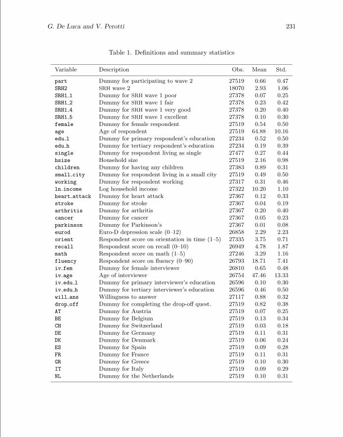
Table 1. Definitions and summary statistics
Variable Description Obs. Mean Std.
part Dummy for participating to wave 2 27519 0.66 0.47SRH2 SRH wave 2 18070 2.93 1.06SRH1 1 Dummy for SRH wave 1 poor 27378 0.07 0.25SRH1 2 Dummy for SRH wave 1 fair 27378 0.23 0.42SRH1 4 Dummy for SRH wave 1 very good 27378 0.20 0.40SRH1 5 Dummy for SRH wave 1 excellent 27378 0.10 0.30female Dummy for female respondent 27519 0.54 0.50age Age of respondent 27519 64.88 10.16edu l Dummy for primary respondent’s education 27234 0.52 0.50edu h Dummy for tertiary respondent’s education 27234 0.19 0.39single Dummy for respondent living as single 27477 0.27 0.44hsize Household size 27519 2.16 0.98children Dummy for having any children 27383 0.89 0.31small city Dummy for respondent living in a small city 27519 0.49 0.50working Dummy for respondent working 27317 0.31 0.46ln income Log household income 27322 10.20 1.10heart attack Dummy for heart attack 27367 0.12 0.33stroke Dummy for stroke 27367 0.04 0.19arthritis Dummy for arthritis 27367 0.20 0.40cancer Dummy for cancer 27367 0.05 0.23parkinson Dummy for Parkinson’s 27367 0.01 0.08eurod Euro-D depression scale (0–12) 26858 2.29 2.23orient Respondent score on orientation in time (1–5) 27335 3.75 0.71recall Respondent score on recall (0–10) 26949 4.78 1.87math Respondent score on math (1–5) 27246 3.29 1.16fluency Respondent score on fluency (0–90) 26793 18.71 7.41iv fem Dummy for female interviewer 26810 0.65 0.48iv age Age of interviewer 26754 47.46 13.33iv edu l Dummy for primary interviewer’s education 26596 0.10 0.30iv edu h Dummy for tertiary interviewer’s education 26596 0.46 0.50will ans Willingness to answer 27117 0.88 0.32drop off Dummy for completing the drop-off quest. 27519 0.82 0.38AT Dummy for Austria 27519 0.07 0.25BE Dummy for Belgium 27519 0.13 0.34CH Dummy for Switzerland 27519 0.03 0.18DE Dummy for Germany 27519 0.11 0.31DK Dummy for Denmark 27519 0.06 0.24ES Dummy for Spain 27519 0.09 0.28FR Dummy for France 27519 0.11 0.31GR Dummy for Greece 27519 0.10 0.30IT Dummy for Italy 27519 0.09 0.29NL Dummy for the Netherlands 27519 0.10 0.31

232 Ordered response models with sample selection
7.1 Sample attrition
In the first two columns of table 2, we compare the probit and SNP estimates of aunivariate binary response model for the probability of participating in wave 2 givenparticipation in wave 1. For the SNP estimator, we considered three alternative specifi-cations obtained by varying the order of the Hermite polynomial expansion (R = 3, 4, 5).For brevity, we present only the estimates of the specification with R = 3, which is theone selected by BIC. As mentioned above, the estimated coefficients of the probit andSNP models are not directly comparable because of the different scale normalizations.Accordingly, we compare ratios of the estimated coefficients by dividing the coefficient ofeach variable by the coefficient of the dummy variable for completing the drop-off ques-tionnaire. The standard errors of these ratios are computed through the delta method(see [R] nlcom).
Table 2. Estimates for the probability of participating in wave 2 given participationin wave 1. Results are based on the normalization |βdrop off| = 1. SNP-estimatedcoefficients of the Hermite polynomial expansions are omitted to save space. * denotesa p-value between 1 and 5%, ** denotes a p-value below 1%. Sample size n1 = 25,278.
Variable probit snp opsel snpopsel
SRH1 1 −0.411 ** −0.421 ** −0.411 ** −0.456 **
SRH1 2 −0.306 ** −0.302 ** −0.306 ** −0.318 **
SRH1 4 −0.036 −0.038 −0.037 −0.069
SRH1 5 0.119 0.108 0.119 0.041
female 0.040 0.039 0.040 0.050
age1 0.010 * 0.010 * 0.010 * 0.010 *
age2 −0.002 ** −0.002 ** −0.002 ** −0.002 **
edu l 0.093 0.101 0.093 0.046
edu h 0.143 0.139 0.143 0.157
single 0.266 ** 0.260 ** 0.268 ** 0.241 **
hsize 0.072 * 0.070 * 0.073 * 0.069
children 0.426 ** 0.413 ** 0.427 ** 0.430 **
small city 0.352 ** 0.338 ** 0.353 ** 0.353 **
working 0.030 0.031 0.030 0.043
ln income −0.051 −0.048 −0.051 −0.079 **
orient 0.114 * 0.120 * 0.114 * 0.078
recall 0.059 ** 0.057 ** 0.059 ** 0.059 **
math −0.001 0.005 −0.001 −0.007
fluency 0.033 ** 0.032 ** 0.033 ** 0.035 **
eurod 0.046 ** 0.044 ** 0.046 ** 0.046 **
heart attack 0.141 0.146 0.142 0.106
stroke 0.247 0.245 0.247 0.263
arthritis 0.242 ** 0.241 ** 0.243 ** 0.244 **
cancer −0.365 ** −0.360 ** −0.363 ** −0.423 **
parkinson −0.368 −0.376 −0.371 −0.361

G. De Luca and V. Perotti 233
iv fem 0.037 0.037 0.031 0.042
iv age1 −0.002 −0.002 −0.002 −0.000
iv age2 −0.000 * −0.000 * −0.000 * −0.000
iv edu l −0.074 −0.070 −0.077 −0.076
iv edu h 0.170 ** 0.167 ** 0.172 ** 0.173 **
will ans 1.166 ** 1.176 ** 1.175 ** 1.149 **
AT −0.001 0.015 −0.007 0.001
BE 0.614 ** 0.601 ** 0.611 ** 0.702 **
CH 0.497 ** 0.504 ** 0.496 ** 0.554 **
DE −0.969 ** −0.958 ** −0.977 ** −0.958 **
DK 0.858 ** 0.829 ** 0.860 ** 0.865 **
ES −0.291 * −0.276 * −0.297 * −0.281 *
FR 0.013 0.021 0.010 0.073
GR 1.518 ** 1.453 ** 1.507 ** 1.808 **
IT 0.552 ** 0.542 ** 0.550 ** 0.590 **
NL −0.309 ** −0.297 * −0.308 * −0.280 *
Skewness 0.382 −0.190
Kurtosis 3.059 3.873
Our estimation results suggest that the relationship between sample attrition andthe health status of the first wave may differ across health dimensions. On the one hand,we find that the attrition probability is negatively associated with cognitive abilities,and it is significantly higher for respondents with a diagnosed cancer and for those withfair and poor SRH1. On the other hand, the attrition probability is significantly lower forrespondents suffering from arthritis and depression problems—probably because theycan be easily traced and approached by the interviewers. Other things being equal,the relationship between the attrition probability and the age of the respondents isU-shaped, with a minimum at 67 years. Furthermore, we find that the attrition proba-bility increases with household income; decreases with household size; and is significantlylower for people who are single, have children, and live in a small city. Coherently withthe findings of the survey nonresponse literature, we also find that interviewer charac-teristics and features of the interview process are important predictors of the attritionprobability. The assumption that the error term follows a Gaussian distribution can-not be rejected by a likelihood ratio test that compares the SNP model with the probitmodel. Once the different scale is taken into account, the differences between probitand SNP estimates are small.
7.2 SRH status
Table 3 presents the estimates of four alternative ordered response models for SRH2,which are labeled with the names of the corresponding Stata commands. oprobit is aunivariate ordered probit model that ignores attrition and assumes Gaussianity of theerror term in the outcome equation. sneop is a univariate SNP ordered response modelthat ignores attrition but relaxes the Gaussian distributional assumption. opsel is
234 Ordered response models with sample selection
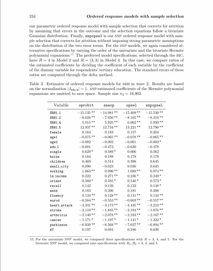
our parametric ordered response model with sample selection that corrects for attritionby assuming that errors in the outcome and the selection equations follow a bivariateGaussian distribution. Finally, snpopsel is our SNP ordered response model with sam-ple selection that corrects for attrition without imposing strong parametric assumptionson the distribution of the two error terms. For the SNP models, we again considered al-ternative specifications by varying the order of the univariate and the bivariate Hermitepolynomial expansions.15 The preferred model specifications, selected through the BIC,have R = 4 in Model 2 and R = (3, 3) in Model 4. In this case, we compare ratios ofthe estimated coefficients by dividing the coefficient of each variable by the coefficientof the dummy variable for respondents’ tertiary education. The standard errors of theseratios are computed through the delta method.
Table 3. Estimates of ordered response models for SRH in wave 2. Results are basedon the normalization |βedu h| = 1. SNP-estimated coefficients of the Hermite polynomialexpansions are omitted to save space. Sample size n2 = 16,902.
Variable oprobit sneop opsel snpopsel
SRH1 1 −15.135 ** −14.981 ** −15.409 ** −15.530 **
SRH1 2 −8.028 ** −7.956 ** −8.165 ** −8.210 **
SRH1 4 5.915 ** 5.925 ** 6.062 ** 5.930 **
SRH1 5 12.937 ** 12.734 ** 13.221 ** 12.790 **
female 0.164 0.183 0.157 0.204
age1 −0.075 ** −0.065 ** −0.078 ** −0.065 **
age2 −0.002 −0.002 −0.001 −0.002 *
edu l −0.601 −0.473 −0.630 −0.478
single 0.629 * 0.589 * 0.606 0.562
hsize 0.184 0.188 0.178 0.178
children 0.469 0.514 0.398 0.645
small city 0.090 −0.023 0.036 0.045
working 1.063 ** 0.996 ** 1.088 ** 0.974 **
ln income 0.222 0.271 ** 0.236 * 0.249 *
orient 0.560 * 0.585 * 0.540 * 0.573 *
recall 0.142 0.139 0.132 0.148 *
math 0.183 0.200 0.181 0.206
fluency 0.134 ** 0.128 ** 0.131 ** 0.134 **
eurod −0.584 ** −0.553 ** −0.603 ** −0.557 **
heart attack −3.331 ** −3.173 ** −3.435 ** −3.219 **
stroke −2.110 ** −1.845 ** −2.194 ** −1.876 **
arthritis −2.140 ** −2.078 ** −2.233 ** −2.107 **
cancer −1.171 * −1.197 * −1.141 * −1.322 *
parkinson −6.939 ** −6.568 ** −7.037 ** −6.894 **
AT 0.197 0.084 0.186 0.038
15. For the univariate SNP model, we compared three specifications with R = 3, 4, and 5. For thebivariate SNP model, we compared nine specifications with R1, R2 = 3, 4, and 5.
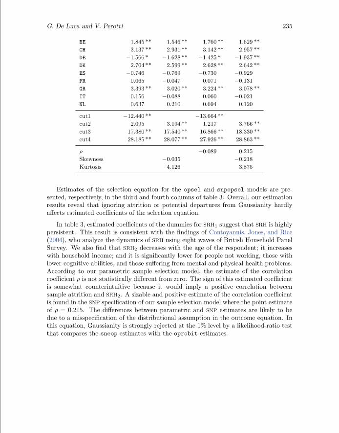
G. De Luca and V. Perotti 235
BE 1.845 ** 1.546 ** 1.760 ** 1.629 **
CH 3.137 ** 2.931 ** 3.142 ** 2.957 **
DE −1.566 * −1.628 ** −1.425 * −1.937 **
DK 2.704 ** 2.599 ** 2.628 ** 2.642 **
ES −0.746 −0.769 −0.730 −0.929
FR 0.065 −0.047 0.071 −0.131
GR 3.393 ** 3.020 ** 3.224 ** 3.078 **
IT 0.156 −0.088 0.060 −0.021
NL 0.637 0.210 0.694 0.120
cut1 −12.440 ** −13.664 **
cut2 2.095 3.194 ** 1.217 3.766 **
cut3 17.380 ** 17.540 ** 16.866 ** 18.330 **
cut4 28.185 ** 28.077 ** 27.926 ** 28.863 **
ρ −0.089 0.215
Skewness −0.035 −0.218
Kurtosis 4.126 3.875
Estimates of the selection equation for the opsel and snpopsel models are pre-sented, respectively, in the third and fourth columns of table 3. Overall, our estimationresults reveal that ignoring attrition or potential departures from Gaussianity hardlyaffects estimated coefficients of the selection equation.
In table 3, estimated coefficients of the dummies for SRH1 suggest that SRH is highlypersistent. This result is consistent with the findings of Contoyannis, Jones, and Rice(2004), who analyze the dynamics of SRH using eight waves of British Household PanelSurvey. We also find that SRH2 decreases with the age of the respondent; it increaseswith household income; and it is significantly lower for people not working, those withlower cognitive abilities, and those suffering from mental and physical health problems.According to our parametric sample selection model, the estimate of the correlationcoefficient ρ is not statistically different from zero. The sign of this estimated coefficientis somewhat counterintuitive because it would imply a positive correlation betweensample attrition and SRH2. A sizable and positive estimate of the correlation coefficientis found in the SNP specification of our sample selection model where the point estimateof ρ = 0.215. The differences between parametric and SNP estimates are likely to bedue to a misspecification of the distributional assumption in the outcome equation. Inthis equation, Gaussianity is strongly rejected at the 1% level by a likelihood-ratio testthat compares the sneop estimates with the oprobit estimates.

236 Ordered response models with sample selection
7.3 Transition probabilities for SRH status
Although ratios of the estimated coefficients provide an easy way of comparing alter-native estimation methods, their interpretation is not always straightforward. Thisstatement explains why in discrete choice models one is usually interested in predictedprobabilities and marginal effects.
In this section, we analyze the implications of the alternative estimation methodsfor the transition probabilities Pr(SRH2 = s | SRH1 = j,X2), s, j = 1, . . . , 5. Theseprobabilities can be easily computed through the margins command by varying thevalues of both the outcome variable SRH2 and the binary indicators for SRH1, whilesetting the variables in X2 to their sample means X2. Below we present an example ofthe Stata codes used to obtain transition probabilities after snpopsel estimation:
. forvalues s=1(1)5 {2. margins, predict(pr outcome(`s´)) noesample
> at((means) _all SRH1_1=1 SRH1_2=0 SRH1_4=0 SRH1_5=0)> at((means) _all SRH1_1=0 SRH1_2=1 SRH1_4=0 SRH1_5=0)> at((means) _all SRH1_1=0 SRH1_2=0 SRH1_4=0 SRH1_5=0)> at((means) _all SRH1_1=0 SRH1_2=0 SRH1_4=1 SRH1_5=0)> at((means) _all SRH1_1=0 SRH1_2=0 SRH1_4=0 SRH1_5=1)> noatlegend
3. matrix snpopsel_`s´=r(b)4. forvalues j=1(1)5 {5. local snpopsel_`j´_`s´=snpopsel_`s´[1,`j´]6. }7. }
Table 4 presents the estimated transition probabilities in SRH for the four modelsconsidered in the previous sections. For each model, the elements on the main diagonalcorrespond to the probabilities of reporting the same health status; those above thediagonal correspond to the probabilities of reporting a better health status; while thosebelow the diagonal correspond to the probabilities of reporting a worse health status.Our estimation results clearly reveal that sample attrition and departures from theparametric distributional assumptions may seriously bias estimates of the transitionprobabilities. For instance, let us focus on the transition probability from poor SRH1
to good SRH2. The estimate from a simple ordered probit model is equal to 18.1%.The parametric correction for sample attrition leads to a slightly higher estimate of19.4%. If sample attrition is associated with a positive survivorship bias, this result issomewhat counterintuitive because we would expect a downward correction of improvinghealth. This is exactly the effect captured by our SNP sample selection model wherethe estimated transition probability is equal to 10.7%. Similar discrepancies can beobserved for most of the other transition probabilities.

G. De Luca and V. Perotti 237
Table 4. Estimates of the transition probabilities for SRH between the first and thesecond waves.
SRH2
Model SRH1 Poor Fair Good V. good Excell.
oprobit Poor 0.320 0.488 0.181 0.011 0.001Fair 0.131 0.455 0.362 0.048 0.004Good 0.031 0.269 0.511 0.158 0.030V. good 0.008 0.135 0.490 0.276 0.091Excell. 0.001 0.042 0.336 0.375 0.246
sneop Poor 0.308 0.534 0.140 0.016 0.003Fair 0.118 0.495 0.335 0.042 0.011Good 0.037 0.250 0.539 0.137 0.036V. good 0.016 0.112 0.504 0.281 0.087Excell. 0.005 0.042 0.300 0.417 0.235
opsel Poor 0.301 0.491 0.194 0.013 0.001Fair 0.121 0.445 0.376 0.053 0.005Good 0.029 0.257 0.514 0.168 0.034V. good 0.007 0.126 0.482 0.286 0.099Excell. 0.001 0.039 0.324 0.377 0.260
snpopsel Poor 0.317 0.560 0.107 0.014 0.001Fair 0.141 0.489 0.330 0.032 0.009Good 0.055 0.237 0.563 0.114 0.031V. good 0.022 0.129 0.497 0.285 0.067Excell. 0.004 0.066 0.284 0.435 0.210
8 Acknowledgments
We thank Franco Peracchi, Claudio Rossetti, and an anonymous referee for helpfulcomments on both the manuscript and the routines. We also thank Mark Stewart forproviding us permission to release an updated version of his sneop command. Thisarticle uses data from release 2 of SHARE 2004 and from release 1 of SHARE 2006.The SHARE data collection has been primarily funded by the European Commissionthrough the Fifth and Sixth Framework Programs, with additional funding from theU.S. National Institute on Aging.
9 ReferencesBorsch-Supan, A., A. Brugiavini, H. Jurges, J. Mackenbach, J. Siegrist, and G. Weber,
ed. 2005. Health, Ageing and Retirement in Europe: First Results from the Survey ofHealth, Ageing and Retirement in Europe. Mannheim: Mannheim Research Institutefor the Economics of Ageing.
238 Ordered response models with sample selection
Chen, S., and S. Khan. 2003. Semiparametric estimation of a heteroskedastic sampleselection model. Econometric Theory 19: 1040–1064.
Contoyannis, P., A. M. Jones, and N. Rice. 2004. The dynamics of health in the Britishhousehold panel survey. Journal of Applied Econometrics 19: 473–503.
Coppejans, M. 2007. On efficient estimation of the ordered response model. Journal ofEconometrics 137: 577–614.
Coppejans, M., and A. R. Gallant. 2002. Cross-validated SNP density estimates. Journalof Econometrics 110: 27–65.
De Luca, G. 2008. SNP and SML estimation of univariate and bivariate binary-choicemodels. Stata Journal 8: 190–220.
De Luca, G., and F. Peracchi. 2010. Estimating models with unit and item nonre-sponse from cross-sectional surveys. EIEF Working Paper 1004, Einaudi Institute forEconomics and Finace.
Dong, Y., and A. Lewbel. 2010. Simple estimators for binary choice models with en-dogenous regressors. Boston College Working Papers in Economics 604, Departmentof Economics, Boston College.
Fitzgerald, J., P. Gottschalk, and R. Moffitt. 1998. An analysis of sample attritionin panel data: The Michigan panel study of income dynamics. Journal of HumanResources 33: 251–299.
Gallant, A. R., and D. W. Nychka. 1987. Semi-nonparametric maximum likelihoodestimation. Econometrica 55: 363–390.
Greene, W. H., and D. A. Hensher. 2009. Modeling ordered choices. Unpublishedmanuscript 1–181.
Keane, M. P. 1992. A note on identification in the multinomial probit model. Journalof Business and Economic Statistics 10: 193–200.
Klein, R. W., and R. P. Sherman. 2002. Shift restrictions and semiparametric estimationin ordered response models. Econometrica 70: 663–691.
Lee, L.-F. 1995. Semiparametric maximum likelihood estimation of polychotomous andsequential choice models. Journal of Econometrics 65: 381–428.
Lewbel, A. 2000. Semiparametric qualitative response model estimation with unknownheteroscedasticity or instrumental variables. Journal of Econometrics 97: 145–177.
Manski, C. F. 1988. Identification of binary response models. Journal of the AmericanStatistical Association 83: 729–738.
Meng, C.-L., and P. Schmidt. 1985. On the cost of partial observability in the bivariateprobit model. International Economic Review 26: 71–85.
G. De Luca and V. Perotti 239
Miranda, A., and S. Rabe-Hesketh. 2006. Maximum likelihood estimation of endogenousswitching and sample selection models for binary, ordinal, and count variables. StataJournal 6: 285–308.
Nicoletti, C., and F. Peracchi. 2005. Survey response and survey characteristics: Mi-crolevel evidence from the European community household panel. Journal of theRoyal Statistical Society, Series A 168: 763–781.
Rabe-Hesketh, S., A. Skrondal, and A. Pickles. 2004. GLLAMM manual. WorkingPaper 160, Division of Biostatistics, University of California–Berkeley.http://www.bepress.com/ucbbiostat/paper160/.
Stewart, M. B. 2004. Semi-nonparametric estimation of extended ordered probit models.Stata Journal 4: 27–39.
———. 2005. A comparison of semiparametric estimators for the ordered responsemodel. Computational Statistics & Data Analysis 49: 555–573.
About the authors
Giuseppe De Luca is a researcher at Istituto per lo Sviluppo della Formazione Professionaledei Lavoratori. Valeria Perotti is a consultant at the World Bank. Each holds a PhD inEconometrics and Empirical Economics from the University of Rome Tor Vergata.

![Overview of Stata estimation commands · [U] 27 Overview of Stata estimation commands3 27.3 Continuous outcomes 27.3.1 ANOVA and ANCOVA ANOVA and ANCOVA fit general linear models](https://static.fdocuments.us/doc/165x107/5e84977f61452326865f32a4/overview-of-stata-estimation-commands-u-27-overview-of-stata-estimation-commands3.jpg)
![Overview of Stata estimation commands · 2[U] 26 Overview of Stata estimation commands Estimation commands share features that this chapter will not discuss; see [U] 20 Estimation](https://static.fdocuments.us/doc/165x107/5ac5c6327f8b9ae06c8df555/overview-of-stata-estimation-commands-u-26-overview-of-stata-estimation-commands.jpg)