Estimation of NIG and VG models for high frequency ...
23
Estimation of NIG and VG models for high frequency financial data Jos´ e E. Figueroa-L´ opez † , Steven R. Lancette † , Kiseop Lee ‡ , and Yanhui Mi † * † Department of Statistics Purdue University W. Lafayette, IN 47907, USA ‡ Department of Mathematics University of Louisville Louisville, KY, 40292, USA and Graduate Department of Financial Engineering Ajou University Suwon, Korea Abstract: Numerous empirical studies have shown that certain exponen- tial L´ evy models are able to fit the empirical distribution of daily financial returns quite well. By contrast, very few papers have considered intraday data in spite of their growing importance. In this paper, we fill this gap by studying the ability of the Normal Inverse Gaussian (NIG) and the Vari- ance Gamma (VG) models to fit the statistical features of intraday data at different sampling frequencies. We propose to assess the suitability of the model by analyzing the signature plots of the point estimates at differ- ent sampling frequencies. Using high frequency transaction data from the U.S. equity market, we find the estimator of the volatility parameter to be quite stable at a wide range of intraday frequencies, in sharp contrast to the estimator of the kurtosis parameter, which is more sensitive to mar- ket microstructure effects. As a secondary contribution, we also assess the performance of the two most favored parametric estimation methods, the Method of Moments Estimators (MME) and the Maximum Likelihood Es- timators (MLE), when dealing with high frequency observations. By Monte Carlo simulations, we show that neither high frequency sampling nor maxi- mum likelihood estimation significantly reduces the estimation error of the volatility parameter of the model. On the contrary, the estimation error of the parameter controlling the kurtosis of log returns can be significantly reduced by using MLE and high-frequency sampling. Both of these results appear to be new in the literature on statistical analysis of high frequency data. Keywords and phrases: Exponential or geometric L´ evy models, High- frequency based estimation, Normal Inverse Gaussian model, Maximum likelihood estimation, Method of moment estimation, Variance Gamma model. * The first author’s research is partially supported by the NSF grant DMS-0906919. The third author’s research is partially supported by WCU (World Class University) program through the National Research Foundation of Korea funded by the Ministry of Education, Science and Technology (R31-20007). 1
Transcript of Estimation of NIG and VG models for high frequency ...

Estimation of NIG and VG models for
high frequency financial data
Jose E. Figueroa-Lopez† , Steven R. Lancette† ,Kiseop Lee‡ , and Yanhui Mi† ∗
†Department of StatisticsPurdue University
W. Lafayette, IN 47907, USA
‡Department of MathematicsUniversity of Louisville
Louisville, KY, 40292, USAand
Graduate Department of Financial EngineeringAjou UniversitySuwon, Korea
Abstract: Numerous empirical studies have shown that certain exponen-tial Levy models are able to fit the empirical distribution of daily financialreturns quite well. By contrast, very few papers have considered intradaydata in spite of their growing importance. In this paper, we fill this gap bystudying the ability of the Normal Inverse Gaussian (NIG) and the Vari-ance Gamma (VG) models to fit the statistical features of intraday dataat different sampling frequencies. We propose to assess the suitability ofthe model by analyzing the signature plots of the point estimates at differ-ent sampling frequencies. Using high frequency transaction data from theU.S. equity market, we find the estimator of the volatility parameter to bequite stable at a wide range of intraday frequencies, in sharp contrast tothe estimator of the kurtosis parameter, which is more sensitive to mar-ket microstructure effects. As a secondary contribution, we also assess theperformance of the two most favored parametric estimation methods, theMethod of Moments Estimators (MME) and the Maximum Likelihood Es-timators (MLE), when dealing with high frequency observations. By MonteCarlo simulations, we show that neither high frequency sampling nor maxi-mum likelihood estimation significantly reduces the estimation error of thevolatility parameter of the model. On the contrary, the estimation error ofthe parameter controlling the kurtosis of log returns can be significantlyreduced by using MLE and high-frequency sampling. Both of these resultsappear to be new in the literature on statistical analysis of high frequencydata.
Keywords and phrases: Exponential or geometric Levy models, High-frequency based estimation, Normal Inverse Gaussian model, Maximumlikelihood estimation, Method of moment estimation, Variance Gammamodel.
∗The first author’s research is partially supported by the NSF grant DMS-0906919. Thethird author’s research is partially supported by WCU (World Class University) programthrough the National Research Foundation of Korea funded by the Ministry of Education,Science and Technology (R31-20007).
1
Figueroa-Lopez et al./Estimation of NIG and VG model for high frequency data 2
1. Introduction
Driven by the necessity to incorporate the observed stylized features of assetprices, continuous-time stochastic modeling has taken a predominant role in thefinancial literature over the past two decades. Most of the proposed models areparticular cases of a stochastic volatility component driven by a Wiener pro-cess superposed with a pure-jump component accounting for the discrete arrivalof major influential information. Accurate approximation of the complex phe-nomenon of trading is certainly attained with such a general model. However,accuracy comes with a high cost in the form of hard estimation and implemen-tation issues as well as over-parameterized models. In practice and certainly forthe purpose motivating the task of modeling in the first place, a parsimoniousmodel with relatively few parameters is desirable. With this motivation in mind,parametric Exponential Levy Models (ELM) are one of the most tractable andsuccessful alternatives to both stochastic volatility models and more general Itosemimartingale models with jumps.
The literature of geometric Levy models is quite extensive (see Cont & Tankov(2004) for a review). Due to their appealing interpretation and tractability,in this work we concentrate on two of the most popular classes: the VarianceGamma (VG) and Normal Inverse Gaussian (NIG) models proposed by Carret al. (1998) and Barndorff-Nielsen (1998), respectively. In the “symmetric case”(which is a reasonable assumption for equity prices), both models require onlyone additional parameter, κ, compared to the two-parameter geometric Brow-nian motion (also called the Black-Scholes model). This additional parametercan be interpreted as the percentage excess kurtosis relative to the normal dis-tribution and, hence, this parameter is mainly in charge of the tail thickness ofthe log return distribution. In other words, this parameter will determine thefrequency of “excessively” large positive or negative returns. Both models arepure jump models with infinite jump activity1. Nevertheless, one of the param-eters, denoted by σ, controls the variability of the log returns and, thus, it canbe interpreted as the volatility of the price process.
Numerous empirical studies have shown that certain parametric exponentialLevy models, including the VG and the NIG models, are able to fit daily returnsextremely well using standard estimation methods such as maximum likelihoodestimators (MLE) or method of moment estimators (MME) (c.f. Eberlein &Keller (1995), Eberlein & Ozkan (2003), Carr et al. (1998), Barndorff-Nielsen(1998), Kou & Wang (2004), Carr et al. (2002), Seneta (2004), Behr & Potter(2009), Ramezani & Zeng (2007), and others). On the other hand, in spite oftheir current importance, very few papers have considered intraday data. Oneof our main motivations in this work is to analyze whether pure Levy modelscan still work well to fit the statistical properties of log returns at the intradaylevel.
As essentially any other model, a Levy model will have limitations when
1That is, a model with infinitely many jumps during any finite time interval [0, T ].
Figueroa-Lopez et al./Estimation of NIG and VG model for high frequency data 3
working with very high-frequency transaction data and, hence, the questionis rather to determine the scales where a Levy model is a good probabilisticapproximation of the underlying (extremely complex and stochastic) tradingprocess. We propose to assess the suitability of the Levy model by analyzingthe signature plots of the point estimates at different sampling frequencies. Itis plausible that an apparent stability of the point estimates for certain rangesof sampling frequencies provides evidence of the adequacy of the Levy modelat those scales. An earlier work along these lines is Eberlein & Ozkan (2003),where this stability was empirically investigated using hyperbolic Levy modelsand MLE (based on hourly data). Concretely, one of the main points therein wasto estimate the model’s parameters from daily mid-day log returns2 and, then,measure the distance between the empirical density based on hourly returns andthe one-hour density implied by the estimated parameters. It is found that thisdistance is approximately minimal among any other implied densities. In otherwords, if fδ(·; θ∗d) denotes the implied density of Xδ when using the parametersθ∗d estimated from daily mid-day returns and if f∗h (·) denotes the empiricaldensity based on hourly returns, then the distance between fδ(·; θ∗d) and f∗h isminimal when δ is approximately one hour. Such a property was termed the“time consistency of Levy processes”.
In this paper, we further investigate the consistency of exponential Levymodels for a wide rage of intraday frequencies using intraday data of the U.S.equity market. Though natural differences due to sampling variation are to beexpected, our empirical results under both models exhibit some very interest-ing common features across the different stocks we analyzed. We find that theestimator of the volatility parameter σ is quite stable for sampling frequenciesas short as 20 minutes or less. For higher frequencies, the volatility estimatesexhibit an abrupt tendency to increase (see Figure 6 below), presumably dueto microstructure effects. In contrast, the kurtosis estimator is more sensitiveto microstructure effects and a certain degree of stability is achieved only formid range frequencies of 1 hour and more (see Figure 6 below). For higherfrequencies, the kurtosis decreases abruptly. In fact, opposite to the smoothsignature plot of σ at those scales, the kurtosis estimates consistently changeby more than half when going from hourly to 30-minute log returns. Again,this phenomenon is presumably due to microstructure effects since the effect ofan unaccounted continuous component will be expected to diminish when thesampling frequency increases.
One of the main motivations of Levy models is that log returns follow idealconditions for statistical inference in that case; namely, under a Levy modelthe log returns at any frequency are independent with a common distribution.Due to this fact, it is arguable that it might be preferable to use a parsimoniousmodel for which efficient estimation is feasible, rather than a very accurate modelfor which estimation errors will be intrinsically large. This is similar to the so-
2These returns are derived from prices recorded in the middle of the trading session. Theidea behind the choice of these prices is to avoid the typically high volatility at the openingand closing of the trading session.

Figueroa-Lopez et al./Estimation of NIG and VG model for high frequency data 4
called model selection problem of statistics where a model with a high numberof parameters typically enjoys a small mis-specification error but suffers from ahigh estimation variance due to the large number of parameters to estimate.
An intrinsic assumption in the previous paragraph is that standard esti-mation methods are indeed efficient in this high frequency data setting. Thisis, however, an overstatement (typically overlooked in the literature) since thepopulation distribution of high-frequency sample data coming from a true Levymodel depends on the sampling frequency itself and, in spite of having moredata, high frequency data does not necessarily imply better estimation results.Hence, another motivation for this work is to analyze the performance of the twomost common estimators, namely the Method of Moments Estimators (MME)and the Maximum Likelihood Estimators (MLE), when dealing with high fre-quency data. As an additional contribution of this analysis, we also proposea simple novel numerical scheme for computing the MME. On the other hand,given the inaccessibility of closed forms for the MLE, we apply an unconstrainedoptimization scheme (Powell’s method) to find them numerically.
By Monte Carlo simulations, we discover the surprising fact that neitherhigh-frequency sampling nor MLE reduces the estimation error of the volatilityparameter in a significant way. In other words, estimating the volatility param-eter based on, say, daily observations has similar performance to doing the samebased on, say, five minute observations. On the other hand, the estimation errorof the parameter controlling the kurtosis of the model can be significantly re-duced by using MLE or intraday data. Another conclusion is that the VG MLEis numerically unstable when working with ultra high frequency data while boththe VG MME and the NIG MLE work quite well for almost any frequency.
The reminder of this article is organized as follows. In Section 2, we review theproperties of the NIG and VG models. Section 3 introduces a simple and novelmethod to compute the moment estimators for the VG and the NIG distribu-tions and also briefly describes the estimation method of maximum likelihood.Section 4 presents the finite-sample performance of the moment estimators andthe maximum likelihood estimator via simulations. In Section 5, we present ourempirical results using high-frequency transaction data from the U.S. equitymarket. The data was obtained from the NYSE TAQ database of 2005 tradesvia Wharton’s WRDS system. For the sake of clarity and space, we only presentthe results for Intel and defer a full analysis of other stocks for a future publi-cation. We finish with a section of conclusions and further recommendations.
2. The statistical models
2.1. Generalities of exponential Levy models
Before introducing the specific models we consider in this paper, let us brieflymotivate the application of Levy processes in financial modeling. We refer the
Figueroa-Lopez et al./Estimation of NIG and VG model for high frequency data 5
reader to the monographs of Cont & Tankov (2004) and Sato (1999) or the re-cent review papers Figueroa-Lopez (2011) and Tankov (2011) for further infor-mation. Exponential (or Geometric) Levy models are arguably the most naturalgeneralization of the geometric Brownian motion intrinsic in the Black-Scholesoption pricing model. A geometric Brownian motion (also called Black-Scholesmodel) postulates the following conditions about the price process (St)t≥0 of arisky asset:
(i) The (log) return on the asset over a time period [t, t+ h] of length h, i.e.
Rt,t+h := logSt+hSt
,
is Gaussian with mean µh and variance σ2h (independent of t);(ii) Log returns on disjoint time periods are mutually independent;(iii) The price path t→ St is continuous; i.e. P(Su → St, as u→ t, for all t) =
1.
The previous assumptions can equivalently be stated in terms of the so-calledlog return process (Xt)t, denoted henceforth as
Xt := logStS0.
Indeed, assumption (i) is equivalent to ask that the increment Xt+h−Xt of theprocess X over [t, t+h] is Gaussian with mean µh and variance σ2h. Assumption(ii) simply means that the increments of X over disjoint periods of time areindependent. Finally, the last condition is tantamount to asking that X hascontinuous paths. Note that we can represent a general geometric Brownianmotion in the form
St = S0eσWt+µt,
where (Wt)t≥0 is the Wiener process. In the context of the above Black-Scholesmodel, a Wiener process can be defined as the log return process of a priceprocess satisfying the Black-Scholes conditions (i)-(iii) with µ = 0 and σ2 = 1.
As it turns out, assumptions (i)-(iii) above are all controversial and believednot to hold true especially at the intraday level (see, e.g., Cont (2001) for aconcise description of the most important features of financial data). The em-pirical distributions of log returns exhibit much heavier tails and higher kurtosisthan a Gaussian distribution does and this phenomenon is accentuated whenthe frequency of returns increases. Independence is also questionable since, e.g.,absolute log returns typically exhibit slowly decaying serial correlation. In otherwords, high-volatility events tend to cluster across time. Of course, continuityis just a convenient limiting abstraction to describe the high trading activityof liquid assets. In spite of its shortcomings, geometric Brownian motion couldarguably be a suitable model to describe low frequency returns but not highfrequency returns.
Figueroa-Lopez et al./Estimation of NIG and VG model for high frequency data 6
An exponential Levy model attempts to relax the assumptions of the Black-Scholes model in a parsimonious manner. Indeed, a natural first step is to relaxthe Gaussian character of log returns by replacing it with an unspecified distri-bution as follows:
(i’) The (log) return on the asset over a time period of length h has distributionFh, depending only on the time span h.
This innocuous (still desirable) change turns out to be inconsistent with con-dition (iii) above in the sense that (ii)-(iii) together with (i’) imply (i). Hence,we ought to relax (iii) as well if we want to keep (i’). The following is a naturalcompromise:
(iii’) The paths t→ St exhibit only discontinuities of first kind (jump disconti-nuities).
Summarizing, a Levy model for the price process (St)t≥0 of a risky asset satisfiesconditions (i’), (ii), and (iii’). In the following section, we concentrate on twoimportant and popular types of Levy models.
2.2. Variance Gamma and Normal Inverse Gaussian models
The Variance Gamma (VG) and Normal Inverse Gaussian (NIG) Levy modelswere proposed in Carr et al. (1998) and Barndorff-Nielsen (1998), respectively,to describe the log return process Xt := logSt/S0 of a financial asset. Bothmodels can be seen as a Wiener process with drift that is time-deformed by anindependent random clock. That is, (Xt) has the representation
Xt = σW (τ(t)) + θτ(t) + bt, (2.1)
where σ > 0, θ, b ∈ R are given constants, W is Wiener process, and τ is asuitable independent subordinator (non-decreasing Levy process) such that
Eτ(t) = t, and Var(τ(t)) = κt.
In the VG model, τ(t) is Gamma distributed with scale parameter β := κ andshape parameter α := t/κ, while in the NIG model τ(t) follows an InverseGaussian distribution with mean µ = 1 and shape parameter λ = 1/(tκ). Inthe formulation (2.1), τ plays the role of a random clock aimed at incorporatingvariations in business activity through time.
The parameters of the model have the following interpretation (see (3.1) and(3.12) below):
1. σ dictates the overall variability of the log returns of the asset; In thesymmetric case (θ = 0), σ2 is the variance of the log returns per unittime;

Figueroa-Lopez et al./Estimation of NIG and VG model for high frequency data 7
2. κ controls the kurtosis or tail heaviness of the log returns; In the symmetriccase (θ = 0), κ is the percentage excess kurtosis of log returns relative tothe normal distribution multiplied by the time span;
3. b is a drift component in calendar time;4. θ is a drift component in business time and controls the skewness of log
returns;
The VG can be written as the difference of two Gamma Levy processes,
Xt = X+t −X−t + bt, (2.2)
where X+ and X− are independent Gamma Levy processes with respectiveparameters
α+ = α− =1
κ, β± :=
√θ2κ2 + 2σ2κ± θκ
2.
One can see X+ (resp. X−) in (2.2) as the upward (resp. downward) movementsin the asset’s log return.
Under both models, the marginal density of Xt (which translates into thedensity of a log return over a time span t) is known in closed form. In the VGmodel, the probability density of Xt is given by
pt(x) =
√2e
θ(x−bt)σ2
σ√πκ
tκΓ( tκ )
|x− bt|√2σ2
κ + θ2
tκ−
12
K tκ−
12
|x− bt|√
2σ2
κ + θ2
σ2
, (2.3)
where K is the modified Bessel function of the second kind (c.f. Carr et al.(1998)). The NIG model has marginal densities of the form
pt(x) =te
tκ+
θ(x−bt)σ2
π
((x− bt)2 + t2σ2
κθ2
κσ2 + 1κ2
)− 12
K1
√
(x− bt)2 + t2σ2
κ
√σ2
κ + θ2
σ2
,
(2.4)
Throughout the paper, we assume that the log return process {Xt}t≥0 issampled during a fixed time interval [0, T ] at evenly spaced times ti = iδn,i = 1, . . . , n, where δn = T/n. This sampling scheme is sometimes called calendartime sampling (c.f. Oomen (2006)). Under the assumption of independence andstationarity of the increments of X (conditions (i’) and (ii) in Section 2.1), wehave at our disposal a random sample
∆ni := ∆n
i X := Xiδn −X(i−1)δn , i = 1, . . . , n, (2.5)
of size n of the distribution fδn(·) := fδn(·;σ, θ, κ, b) of Xδn . Note that, in thiscontext, a larger sample size n does not necessarily entail a greater amount ofuseful information about the parameters of the model. This is, in fact, one ofthe key questions in this paper: does the statistical performance of standardparametric methods improve under high-frequency observations? We will ad-dress this issue by simulation experiments in Section 4. For now, we introducethe statistical methods used in this article.
Figueroa-Lopez et al./Estimation of NIG and VG model for high frequency data 8
3. Parametric estimation methods
In this part, we review the most used parametric estimation methods: themethod of moments and maximum likelihood. We also present a new com-putational method to find the moment estimators of the considered models.It is worth pointing out that both methods are known to be consistent undermild conditions if the number of observations at a fixed frequency (say, daily orhourly) are independent.
3.1. Method of moment estimators
In principle, the method of moments is a simple estimation method that canbe applied to a wide range of parametric models. Also, the method of momentestimators (MME) are commonly used as initial points of numerical schemesused to find Maximum Likelihood Estimators (MLE), which are typically con-sidered to be more efficient. Another appealing property of moment estimatorsis that they are known to be robust against possible dependence between logreturns since their consistency is only a consequence of stationarity and ergod-icitity conditions of the log returns. In this section, we introduce a new methodto compute the MME for the VG and NIG models.
Let us start with the VG model. The mean and first three central momentsof a VG model are given in closed form as follows (see, e.g., Cont & Tankov,2004, pp. 32 & 117):
µ1(Xδ) := E(Xδ) = (θ + b)δ,
µ2(Xδ) := Var(Xδ) = (σ2 + θ2κ)δ, (3.1)
µ3(Xδ) := E(Xδ − EXδ)3 = (3σ2θκ+ 2θ3κ2)δ,
µ4(Xδ) := E(Xδ − EXδ)4 = (3σ4κ+ 12σ2θ2κ2 + 6θ4κ3)δ + 3µ2(Xδ)
2.
The MME is obtained by solving the system of equations resulting fromsubstituting the central moments of Xδn in (3.1) by their corresponding sampleestimators:
µk,n :=1
n
n∑i=1
(∆ni − ∆(n)
)k, k ≥ 2, (3.2)
where ∆ni is given as in (2.5) and ∆(n) :=
∑ni=1 ∆n
i /n. However, solving thesystem of equations that defines the MME is not straightforward and, in general,one will need to rely on a numerical solution of the system. We now describe anovel simple method for this purpose. The idea is to write the central momentsin terms of the quantity E := θ2κ/σ2. Concretely, we have the equations
µ2(Xδ) = δσ2(1 + E), µ3(Xδ) = δσ2θκ(3 + 2E),
µ4(Xδ)
3µ22(Xδ)
− 1 =κ
δ
1 + 4E + 2E2
(1 + E)2.

Figueroa-Lopez et al./Estimation of NIG and VG model for high frequency data 9
From these equations, it follows that
3µ23(Xδ)
µ2(Xδ) (µ4(Xδ)− 3µ22(Xδ))
=E (3 + 2E)
2
(1 + 4E + 2E2) (1 + E):= f(E). (3.3)
In spite of appearances, the above function f(E) is a strictly increasing concavefunction from (−1 + 2−1/2,∞) onto (−∞, 2) and, hence, the solution of the cor-responding sample equation can be found efficiently using numerical methods.It remains to estimate the left hand side of (3.3). To this end, note that theleft-hand side term can be written as 3Skw(Xδ)
2/Krt(Xδ), where Skw and Krtrepresent the population skewness and kurtosis:
Skw(Xδ) :=µ3(Xδ)
µ2(Xδ)3/2, Krt(Xδ) :=
µ4(Xδ)
µ2(Xδ)2− 3. (3.4)
Finally, we just have to replace the population parameters by their empiricalestimators:
Varn :=1
n− 1
n∑i=1
(∆ni − ∆n
)2, Skwn :=
µ3,n
µ3/22,n
, Krtn :=µ4,n
µ22,n
− 3. (3.5)
Summarizing, the MME can be computed via the following numerical scheme:
1. Find (numerically) the solution E∗n of the equation
f(E) =3 Skw
2
n
Krtn; (3.6)
2. Determine the MME using the following formulas:
σ2n :=
Varnδn
(1
1 + E∗n
), κn :=
δn3
Krtn
((1 + E∗n)2
1 + 4E∗n + 2E∗n2
), (3.7)
θn :=µ3,n
δnσ2nκn
(1
3 + 2E∗n
), bn :=
1
δn∆n − θn =
XT
T− θn. (3.8)
We note that the above estimators will exist if and only if the equation (3.6)admits a solution E∗ ∈ (−1 + 2−1/2,∞), which is the case if and only if
3 Skw2
n
Krtn< 2.
Furthermore, the MME estimator κn will be positive only if the sample kurtosisKrtn is positive. It turns out that in simulations this condition is sometimesviolated for small time horizons T and coarse sampling frequencies (say, dailyor longer). For instance, using the parameter values (i) of Section 4.1 below andtaking T = 125 days (half a year) and δn = 1 day, about 80 simulations out of
Figueroa-Lopez et al./Estimation of NIG and VG model for high frequency data 10
1000 gave invalid κ, while only 2 simulations result in invalid κ when δn = 1/2day.
Seneta (2004) proposes a simple approximation method built on the assump-tion that θ is typically small. In our context, Seneta’s method is obtained bymaking the simplifying approximation E∗n ≈ 0 in the equations (3.7-3.8), result-ing in the following estimators:
σ2n :=
Varnδn
, κn :=δn3
Krtn, (3.9)
θn :=µ3,n
3δnσ2nκn
=Skwn(Varn)1/2
δnKrtn, bn :=
XT
T− θn. (3.10)
Note that the estimators (3.9) are, in fact, the actual MME in the restrictedsymmetric model θ = 0 and will indeed produce a good approximation of theMME estimators (3.7-3.8) whenever
Q∗n :=3 Skw
2
n
Krtn,
and, hence, E∗n is “very” small. This fact has been corroborated empirically bymultiple studies using daily data as shown in Seneta (2004).
The formulas (3.9-3.10) have appealing interpretations as noted already byCarr et al. (1998). Namely, the parameter κ determines the percentage excesskurtosis in the log return distribution (i.e. a measure of the tail fatness comparedto the normal distribution), σ dictates the overall volatility of the process, and θdetermines the skewness. Interestingly, the estimator σ2
n in (3.9) can be writtenas
σ2n =
1
T − δn
n∑i=1
(Xiδn −X(i−1)δn −
XT
n
)2
=1
T − δnRV n +O
(1
n
),
where RV n is the well-known realized variance defined by
RV n :=
n∑i=1
(Xiδn −X(i−1)δn
)2. (3.11)
Let us finish this section by considering the NIG model. In this setting, themean and first three central moments are given by (see, e.g., Cont & Tankov,2004, pp. 117):
µ1(Xδ) := E(Xδ) = (θ + b)δ,
µ2(Xδ) := Var(Xδ) = (σ2 + θ2κ)δ, (3.12)
µ3(Xδ) := E(Xδ − EXδ)3 = (3σ2θκ+ 3θ3κ2)δ,
µ4(Xδ) := E(Xδ − EXδ)4 = (3σ4κ+ 18σ2θ2κ2 + 15θ4κ3)δ + 3µ2(Xδ)
2.
Figueroa-Lopez et al./Estimation of NIG and VG model for high frequency data 11
Hence, the equation (3.3) takes the simpler form:
3µ23(Xδ)
µ2(Xδ) (µ4(Xδ)− 3µ22(Xδ))
=9E
5E + 1:= f(E), (3.13)
and the analogous equation (3.6) can be solved in closed form as
E∗n =Skw
2
n
3 Krtn − 5 Skw2
n
. (3.14)
Then, the MME will be given by the following formulas:
σ2n :=
Varnδn
(1
1 + E∗n
), κn :=
δn3
Krtn
(1 + E∗n1 + 5E∗n
), (3.15)
θn :=µ3,n
δnσ2nκn
(1
3 + 3E∗n
), bn :=
1
δn∆n − θn =
XT
T− θn. (3.16)
3.2. Maximum likelihood estimation
Maximum likelihood is one of the most widely used estimation methods, partlydue to its theoretical efficiency when dealing with large samples. Given a ran-dom sample x = (x1, . . . , xn) from a population distribution with density f(·|θ)depending on a parameter θ = (θ1, . . . , θp), the method proposes to estimate θ
with the value θ = θ(x) that maximizes the so-called likelihood function
L(θ|x) :=
n∏i=1
f(xi|θ).
When it exists, such a point estimate θ(x) is called the Maximum LikelihoodEstimator (MLE) of θ.
In principle, under a Levy model, the increments of the log return process X(which corresponds to the log returns of the price process S) are independentwith common distribution, say fδ(·|θ), where δ represents the time span ofthe increments. As was pointed out earlier, independence is questionable forvery high frequency log returns, but given that, for a large sample, likelihoodestimation is expected to be robust against small dependences between returns,we can still apply likelihood estimation. The question is again to determine thescales where both the Levy model is a good approximation of the underlyingprocess and the maximum likelihood estimators are meaningful. As indicatedin the introduction, it is plausible that the MLE’s stability for certain range ofsampling frequencies provides evidence of the adequacy of the Levy model atthose scales.
Another important issue is that, in general, the probability density fδ is notknown in a closed form or might be intractable. There are several approaches

Figueroa-Lopez et al./Estimation of NIG and VG model for high frequency data 12
to deal with this issue such as numerically inverting the Fourier transform offδ via Fast Fourier Methods (see Carr et al. (2002)) or approximating fδ us-ing small-time expansions (see, e.g., Figueroa-Lopez & Houdre (2009)). In thepresent article, we don’t explore these approaches since the probability densi-ties of the VG and NIG models are known in closed forms. However, given theinaccessibility of closed expressions for the MLE, we apply an unconstrainedoptimization scheme to find them numerically (see below for more details).
4. Finite-sample performance via simulations
4.1. Parameter values
We consider two sets of parameter values:
(i) σ =√
6.447 ∗ 10−5 = .0080; κ = 0.422; θ = −1.5∗10−4; b = 2.5750∗10−4;(ii) σ = .0127; κ = 0.2873; θ = 1.3 ∗ 10−3; b = −1.7 ∗ 10−3;
The first set of parameters (i) is motivated by the empirical study reported inSeneta (2004) (see pp. 182) using the approximated MME introduced in Section3.1 and daily returns of the Standard and Poor’s 500 Index from 1977 to 1981.The second set of parameters (ii) is motivated by our own empirical results belowusing MLE and daily returns of INTC during 2005. Throughout, the time unitis a day and, hence, e.g., the estimated average rate of return per day of SP500is
EX(1) = E log
(S1
S0
)= θ + b = 1.0750 ∗ 10−4 ≈ .1%,
or 0.00010750 ∗ 365 = 3.9% per year.
4.2. Results
Below, we illustrate the finite-sample performance of the MME and MLE forboth the VG and NIG models. The MME is computed using the algorithms de-scribed in Section 3.1. The MLE was computed using an unconstrained Powell’smethod3 started at the exact MME. We use the closed form expressions for thedensity functions (2.3-2.4) in order to evaluate the likelihood function.
4.2.1. Variance Gamma
We compute the sample mean and sample standard deviation of the VG MMEand the VG MLE for different sampling frequencies. Concretely, the time span δ
3We employ a MATLAB implementation due to Giovani Tonel obtained through MATLABCentral (http://www.mathworks.com/matlabcentral/fileexchange/).

Figueroa-Lopez et al./Estimation of NIG and VG model for high frequency data 13
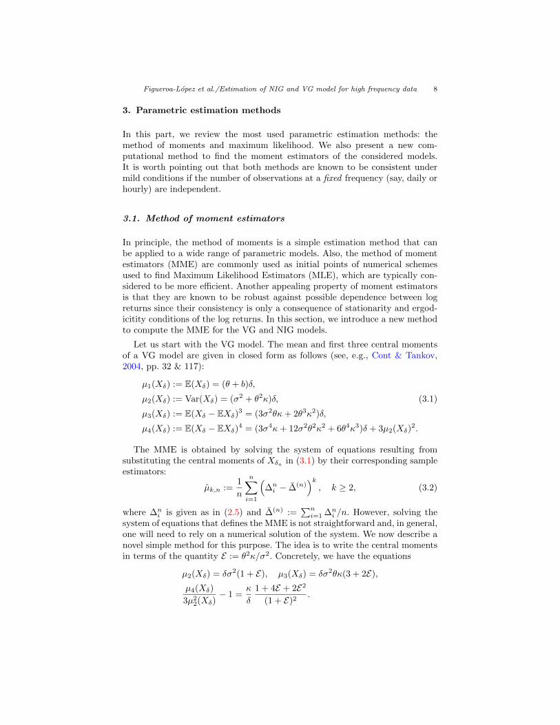
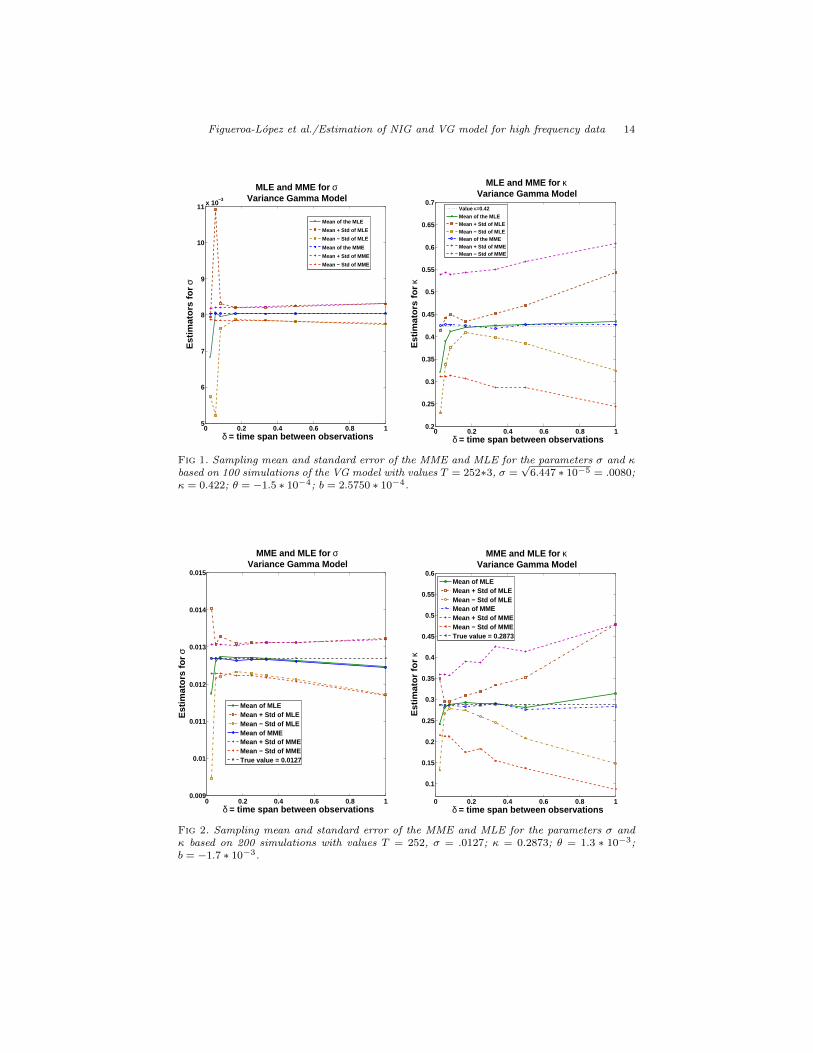
between consecutive observations is taken to be 1/36, 1/18, 1/12, 1/6, 1/3, 1/2, 1(in days), which will correspond to 10, 20, 30 minutes, 1, 2, 3 hours and 1 day(assuming a trading period of six hours per day). Figure 1 plots the samplingmean ¯σδ and the bands ¯σδ ± std(σδ) against the different time spans δ as wellas the corresponding graphs for κ, based on 100 simulations of the VG processon [0, 3 ∗ 252] (namely, 3 years) with the parameter values (i) above. Similarly,Figure 2 shows the results corresponding to the parameter values (ii) with a timehorizon of T = 252 days and time spans δ equal to 10, 20, and 30 minutes, andalso, 1/6, 1/4, 1/3, 1/2, and 1 days, assuming this time a trading period of sixand a half hours per day and taking 200 simulations. These are our conclusions:
1. The MME for σ performs as well as the computationally more expensiveMLE for all the relevant frequencies. Even though increasing the samplingfrequency slightly reduces the standard error, the net gain is actually verysmall even for very high frequencies and, hence, does not justify the useof high-frequency data to estimate σ.
2. The estimation for κ is quite different: Using either high-frequency dataor maximum likelihood estimation results in significant reductions of thestandard error (by more than 4 times when using both).
3. The computation of the MLE presents numerical issues (easy to detect)for very high sampling frequencies (say δ < 1/6).
4. Disregarding the numerical issues and extrapolating the pattern of thegraphs when δ → 0, we can conjecture that the MLE σ is not consistentwhen δ → 0 for a fixed time horizon T , while the MLE κ appears to be aconsistent estimator for κ. Both of these points will be investigated in afuture publication.
For completeness, we also illustrates in Figure 3 the performance of the esti-mators for b and θ for the parameter values (ii) based again on 200 simulationsduring [0, 252] with time spans of 10, 20, and 30 minutes, and 1/6, 1/4, 1/3,1/2, and 1 days. There seems to be some gain in efficiency when using MLEand higher sampling frequencies in both cases but the respective standard errorslevel off for δ small, suggesting that neither estimator is consistent for fixed timehorizon. One surprising feature is that the MLE estimators in both cases do notseem to exhibit any numerical issues for very small δ in spite of being based onthe same simulations as those used to obtain σ and κ.
4.2.2. Normal Inverse Gaussian
We now show the estimation results for the NIG model. Here, we take samplingfrequencies of 5, 10, 20, and 30 seconds, also 1, 5, 10, 20, and 30 minutes, aswell as 1, 2, and 3 hours, and finally 1 day (assuming a trading period of 6hours). Figure 4 plots the sampling mean ¯σδ and bands ¯σδ ± std(σδ) againstthe different time spans δ andthe corresponding graphs for κ, based on 100simulations of the NIG process on [0, 3 ∗ 252] with the parameter values (i)
Figueroa-Lopez et al./Estimation of NIG and VG model for high frequency data 14
0 0.2 0.4 0.6 0.8 15
6
7
8
9
10
11 x 10−3
δ = time span between observations
Est
imat
ors
for
σMLE and MME for σ
Variance Gamma Model
Mean of the MLE
Mean + Std of MLE
Mean − Std of MLE
Mean of the MME
Mean + Std of MME
Mean − Std of MME
0 0.2 0.4 0.6 0.8 10.2
0.25
0.3
0.35
0.4
0.45
0.5
0.55
0.6
0.65
0.7
δ = time span between observations
Est
imat
ors
for
κ
MLE and MME for κVariance Gamma Model
Value κ=0.42Mean of the MLEMean + Std of MLEMean − Std of MLEMean of the MMEMean + Std of MMEMean − Std of MME
Fig 1. Sampling mean and standard error of the MME and MLE for the parameters σ and κbased on 100 simulations of the VG model with values T = 252∗3, σ =
√6.447 ∗ 10−5 = .0080;
κ = 0.422; θ = −1.5 ∗ 10−4; b = 2.5750 ∗ 10−4.
0 0.2 0.4 0.6 0.8 10.009
0.01
0.011
0.012
0.013
0.014
0.015
MME and MLE for σVariance Gamma Model
δ = time span between observations
Est
imat
ors
for
σ
Mean of MLEMean + Std of MLEMean − Std of MLEMean of MMEMean + Std of MMEMean − Std of MMETrue value = 0.0127
0 0.2 0.4 0.6 0.8 1
0.1
0.15
0.2
0.25
0.3
0.35
0.4
0.45
0.5
0.55
0.6
MME and MLE for κVariance Gamma Model
δ = time span between observations
Est
imat
or fo
r κ
Mean of MLEMean + Std of MLEMean − Std of MLEMean of MMEMean + Std of MMEMean − Std of MMETrue value = 0.2873
Fig 2. Sampling mean and standard error of the MME and MLE for the parameters σ andκ based on 200 simulations with values T = 252, σ = .0127; κ = 0.2873; θ = 1.3 ∗ 10−3;b = −1.7 ∗ 10−3.
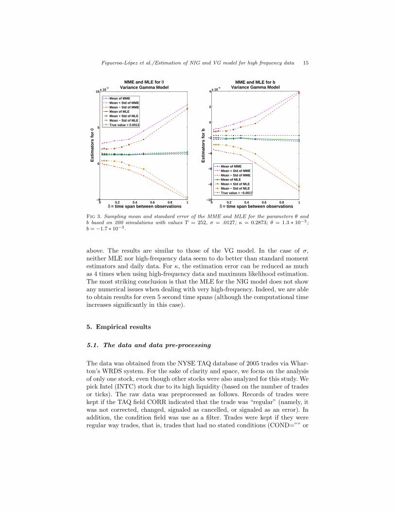
Figueroa-Lopez et al./Estimation of NIG and VG model for high frequency data 15
0 0.2 0.4 0.6 0.8 1−5
0
5
10 x 10−3
MME and MLE for θVariance Gamma Model
δ = time span between observations
Est
imat
ors
for
θ
Mean of MMEMean + Std of MMEMean − Std of MMEMean of MLEMean + Std of MLEMean − Std of MLETrue value = 0.0013
0 0.2 0.4 0.6 0.8 1−10
−8
−6
−4
−2
0
2
4 x 10⁻³
δ = time span between observationsE
stim
ator
s fo
r b
MME and MLE for bVariance Gamma Model
Mean of MMEMean + Std of MMEMean − Std of MMEMean of MLEMean + Std of MLEMean − Std of MLETrue value = −0.0017
Fig 3. Sampling mean and standard error of the MME and MLE for the parameters θ andb based on 200 simulations with values T = 252, σ = .0127; κ = 0.2873; θ = 1.3 ∗ 10−3;b = −1.7 ∗ 10−3.
above. The results are similar to those of the VG model. In the case of σ,neither MLE nor high-frequency data seem to do better than standard momentestimators and daily data. For κ, the estimation error can be reduced as muchas 4 times when using high-frequency data and maximum likelihood estimation.The most striking conclusion is that the MLE for the NIG model does not showany numerical issues when dealing with very high-frequency. Indeed, we are ableto obtain results for even 5 second time spans (although the computational timeincreases significantly in this case).
5. Empirical results
5.1. The data and data pre-processing
The data was obtained from the NYSE TAQ database of 2005 trades via Whar-ton’s WRDS system. For the sake of clarity and space, we focus on the analysisof only one stock, even though other stocks were also analyzed for this study. Wepick Intel (INTC) stock due to its high liquidity (based on the number of tradesor ticks). The raw data was preprocessed as follows. Records of trades werekept if the TAQ field CORR indicated that the trade was “regular” (namely, itwas not corrected, changed, signaled as cancelled, or signaled as an error). Inaddition, the condition field was use as a filter. Trades were kept if they wereregular way trades, that is, trades that had no stated conditions (COND=”” or

Figueroa-Lopez et al./Estimation of NIG and VG model for high frequency data 16
0 0.1 0.2 0.3 0.4 0.5 0.6 0.7 0.8 0.9 17.4
7.6
7.8
8
8.2
8.4
8.6x 10⁻³
δ = time span between observations
Est
imat
ors
for
σ
MLE and MME for σNormal Inverse Gaussian
Value=sqrt of .00006447Mean of MMEMean + Std of MMEMean − Std of MMEMean of MLEMean + Std of MLEMean − Std of MLE
0 0.1 0.2 0.3 0.4 0.5 0.6 0.7 0.8 0.9 10.1
0.2
0.3
0.4
0.5
0.6
0.7
0.8
δ = time span between observationsE
stim
ator
s fo
r κ
MME and MLE for κNormal Inverse Gaussian
True value = 0.442Mean of MMEMean + Std of MMEMean − Std of MMEMean of MLEMean + Std of MLEMean − Std of MLE
Fig 4. Sampling mean and standard error of the MME and MLE for the parameters σ andκ based on 100 simulations of the NIG model with values T = 252 ∗ 3, σ =
√6.447 ∗ 10−5 =
.0080; κ = 0.422; θ = −1.5 ∗ 10−4; b = 2.5750 ∗ 10−4.
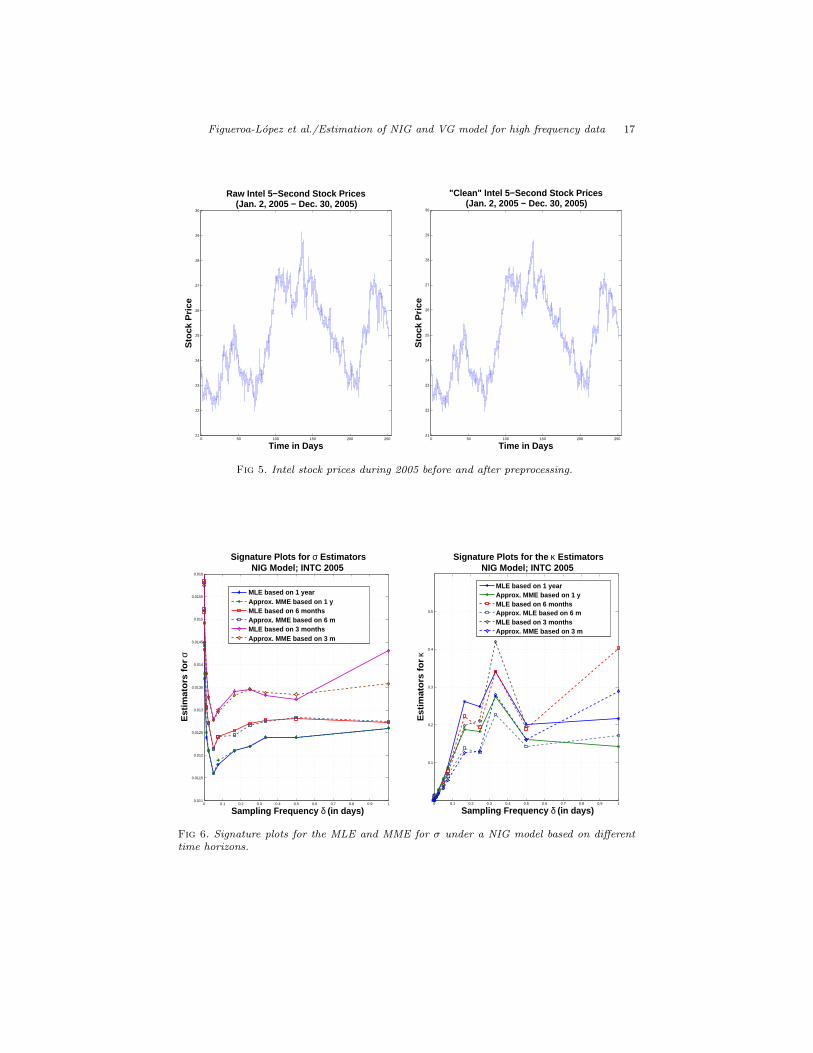
COND=”*”). A secondary filter was subsequently applied to eliminate some ofthe remaining incorrect trades. First, for each trading day, the empirical distri-bution of the absolute value of the first difference of prices was determined. Next,the 99.9th percentile of these daily absolute differences was obtained. Finally, atrade was eliminated if, in magnitude, the difference of the price from the priorprice was at least twice the 99.9th percentile of that day’s absolute differencesand this difference was reversed on the following trade. Figure 5 illustrates theIntel stock prices before (left panel) and after processing (right panel).
5.2. MME and MLE results
The exact and approximated MMEs described in Section 3.1 were applied to thelog returns of the stocks at different frequencies ranging from 10 seconds up to1 day. Subsequently, we apply the unconstrained Powell’s optimization methodto find the MLE estimator. In each case, the starting point for the optimizationroutine was set equal to the exact MME. Tables 1 to 4 show the estimationresults under both models together with the log likelihood values using a timehorizon of one year. Figure 6 show the graphs of the NIG MLE and approximatedNIG MME against the sampling frequency δ based on observations during T = 1year, T = 6 months, and T = 3 months, respectively.
Figueroa-Lopez et al./Estimation of NIG and VG model for high frequency data 17
0 50 100 150 200 25021
22
23
24
25
26
27
28
29
30
Raw Intel 5−Second Stock Prices(Jan. 2, 2005 − Dec. 30, 2005)
Time in Days
Sto
ck P
rice
0 50 100 150 200 25021
22
23
24
25
26
27
28
29
30
"Clean" Intel 5−Second Stock Prices(Jan. 2, 2005 − Dec. 30, 2005)
Time in Days
Sto
ck P
rice
Fig 5. Intel stock prices during 2005 before and after preprocessing.
0 0.1 0.2 0.3 0.4 0.5 0.6 0.7 0.8 0.9 10.011
0.0115
0.012
0.0125
0.013
0.0135
0.014
0.0145
0.015
0.0155
0.016
Signature Plots for σ EstimatorsNIG Model; INTC 2005
Sampling Frequency δ (in days)
Est
imat
ors
fo
r σ
MLE based on 1 yearApprox. MME based on 1 yMLE based on 6 monthsApprox. MME based on 6 mMLE based on 3 monthsApprox. MME based on 3 m
0 0.1 0.2 0.3 0.4 0.5 0.6 0.7 0.8 0.9 10
0.1
0.2
0.3
0.4
0.5
Signature Plots for the κ EstimatorsNIG Model; INTC 2005
Sampling Frequency δ (in days)
Est
imat
ors
fo
r κ
MLE based on 1 yearApprox. MME based on 1 yMLE based on 6 monthsApprox. MLE based on 6 mMLE based on 3 monthsApprox. MME based on 3 m
Fig 6. Signature plots for the MLE and MME for σ under a NIG model based on differenttime horizons.

Figueroa-Lopez et al./Estimation of NIG and VG model for high frequency data 18
5.3. Discussion of empirical results
In spite of certain natural differences due to sampling variation, the empiricalresults under both models exhibit some very interesting common features thatwe now summarize:
1. The estimation of σ is quite stable for “midrange” frequencies (δ ≥ 20minutes), exhibiting a slight tendency to decrease when δ decreases from1 day to 10 minutes, before showing a pronounce and clear tendency toincrease for small time spans (δ = 10 minutes and less). This increasingtendency is presumably due to the influence of microstructure effects.
2. The point estimators for κ are less stable than those for σ but still theirvalues are relatively “consistent” for mid range frequencies of 1 hour andmore. This consistency of κ abruptly changes when δ moves from 1/6 of aday to 30 minutes, at which point a reduction of about half is experiencedunder both models. To illustrate how unlikely such a behavior is in ourmodels, we consider the simulation experiment of Figure 2 and find outthat in only 1 out of the 200 simulations the exact MME estimator for κincreased by more than twice its value when δ goes from 30 minutes to 1/6of a day (only 3 out 200 simulations showed an increment of more than1.5). In none of the 200 simulation, the MLE estimator for κ increasedmore than 1.5 its value when δ goes from 30 minutes to 1/6 of a day. Forthe NIG model, using the simulations of Figure 4, we found out that inonly 3 out 100 simulations the MME estimator for κ increased by morethan 1.2 when δ goes from 30 minutes to 1/6 of a day (it never increased formore than 1.5). Such a jump in the empirical results could be interpretedas a consequence of microstructure effects;
3. According to our previous simulation analysis, the estimators for κ aremore reliable when δ gets smaller. Hence, we recommend using the valueof the estimator for δ as small as possible, but still in the range where wesuspect that microstructure effects are relatively low. For instance, one canpropose to take κ = 0.1662 under the VG model (resp. κ = 0.2621 underthe NIG model), or alternatively, one could average the MLE estimatorsfor δ > 1/2.
4. Under both models, the estimators for κ show a certain tendency to de-crease as δ gets very small (less than 30 minutes).
5. Given the higher sensitivity of κ to microstructure effects, one could usethe values of this estimator to identify the range of frequencies where aLevy model is adequate and microstructure effects are still low. In the caseof INTC, one can recommend using a Levy model to describe log returnshigher than one hour. As an illustration of the goodness of fit, Figures 7shows the empirical histograms of δ = 1/6 returns against the fitted VGmodel and NIG model using Maximum Likelihood Estimation. We alsoshow the fitted Gaussian distributions in each case. Both models showvery good fit. The graphs in log scale, useful to check the fit at the tails,are shown in Figure 8.

Figueroa-Lopez et al./Estimation of NIG and VG model for high frequency data 19
6. Conclusion
Certain parametric classes of exponential Levy models have appealing featuresfor modeling intraday financial data. In this article, we lean towards choosinga parsimonious model with few parameters that has natural financial inter-pretation, rather than a complex over-parameterized model. Even though, inprinciple, a complex model will provide a better fit of the observed empiricalfeatures of financial data, the intrinsically less accurate estimation or calibrationof such a model might render it less useful in practice. By contrast, we considerhere two simple and well-known models for the analysis of intraday data: theVariance Gamma model of Carr et al. (1998) and the Normal Inverse Gaussianmodel of Barndorff-Nielsen (1998). These models require one additional param-eter, when compared to the two-parameter Black-Scholes model, that controlsthe tail thickness of the log return distribution.
As essentially any other model, a Levy model will have limitations whenworking with very high-frequency transaction data and, hence, in our opinion thereal problem is to determine the sampling frequencies at which a specific Levymodel will be a “good” probabilistic approximation of the underlying tradingprocess. In this paper we put forward an intuitive statistical method to solve thisproblem. Concretely, we propose to assess the suitability of the Levy model byanalyzing the signature plots of statistical point estimates at different samplingfrequencies. It is plausible that an apparent stability of the point estimates forcertain ranges of sampling frequencies will provide evidence of the adequacy ofthe Levy model at those scales. At least based on our preliminary empiricalanalysis, we find that a Levy model seems a reasonable model for log returns asfrequent as hourly and that the kurtosis estimate is a more sensitive indicatorof microstructure effects in the data than the volatility estimate, which exhibitsa very stable behavior for sampling time spans as small as 20 minutes.
We also studied the in-fill numerical performance of the two most widely usedparametric estimators: the method of moment estimators and the maximumlikelihood estimation. We discover that neither high frequency sampling normaximum likelihood estimation significantly reduces the estimation error of thevolatility parameter of the model. Hence, we can “safely” estimate the volatilityparameter using a simple moment estimator applied to daily closing prices. Theestimation of the kurtosis parameter is quite different. In that case, using eitherhigh-frequency data or maximum likelihood estimation can result in significantreductions of the standard error (by more than 4 times when using both). Bothof these results appear to be new in the statistical literature of high frequencydata.
The problem of finding the MLE based on very high frequency data remainsa challenging numerical problem, even if closed form expressions are availableas it is the case of the NIG and VG models. On the contrary, in this paper,we propose a simple numerical method to find the MME of the NIG and VGmodels. Moment estimators are particularly appealing in the context of high-

Figueroa-Lopez et al./Estimation of NIG and VG model for high frequency data 20
frequency data since their consistency does not require independence betweenlog returns but only stationarity and ergodicity conditions.
δ 20 min 30 min 1/6 1/4 1/3 1/2 1κ 0.0354 0.0542 0.1662 0.1724 0.2342 0.2098 0.2873σ 0.0115 0.0117 0.0120 0.0121 0.0123 0.0125 0.0127
θ 0.0010 0.0023 0.0019 0.0011 0.0020 0.0020 0.0013
b -0.0014 -0.0027 -0.0023 -0.0015 -0.0024 -0.0023 -0.0017logL 2.2485e+4 1.4266e+4 6.0015e+3 3.7580e+3 2.6971e+3 1.6783e+3 745.8689κ 0.0571 0.0834 0.1839 0.1804 0.2694 0.1579 0.1383σ 0.0116 0.0119 0.0120 0.0121 0.0123 0.0124 0.0125
θ 0.0016 0.0010 0.0032 0.0019 0.0024 0.0028 0.0041
b -0.0020 -0.0014 -0.0036 -0.0022 -0.0028 -0.0032 -0.0045logL 2.2438e+4 1.4243e+4 5.9946e+3 3.7578e+3 2.6966e+3 1.6780e+3 745.5981κ 0.0573 0.0835 0.1887 0.1819 0.2749 0.1603 0.1423σ 0.0116 0.0119 0.0121 0.0122 0.0124 0.0124 0.0126
θ 0.0016 0.0010 0.0031 0.0018 0.0024 0.0027 0.0040
b -0.0020 -0.0014 -0.0035 -0.0022 -0.0027 -0.0031 -0.0043logL 2.2437e+4 1.4243e+4 5.9942e+3 3.7577e+3 2.6965e+3 1.6781e+3 745.6023
Table 1INTC: VG MLE (Top), Exact VG MME (Middle), and Approx. VG MME (Bottom).
δ 10 sec 20 sec 30 sec 1 min 5 min 10 minκ 0.0128 0.0112 0.0183 0.0354 0.0501 0.0191σ 0.0465 0.0300 0.0303 0.0293 0.0173 0.0120
θ -0.0004 -0.0004 -0.0004 -0.0004 -0.0004 -0.0002
b 0.0000 -0.0000 0.0000 0.0000 0.0000 -0.0002logL 5.2980e+6 2.4338e+6 1.5115e+6 6.6256e+5 1.0540e+5 4.7949e+4κ 0.0010 0.0023 0.0052 0.0080 0.0153 0.0282σ 0.0169 0.0152 0.0145 0.0138 0.0125 0.0121
θ -0.0001 0.0014 0.0025 -0.0040 -0.0013 0.0011
b -0.0003 -0.0018 -0.0029 0.0036 0.0009 -0.0015logL 4.3254e+6 2.0063e+6 1.2823e+6 5.8998e+5 1.0203e+5 4.7897e+4κ 0.0010 0.0023 0.0052 0.0081 0.0153 0.0282σ 0.0169 0.0152 0.0145 0.0138 0.0125 0.0121
θ -0.0001 0.0014 0.0025 -0.0040 -0.0013 0.0011
b -0.0003 -0.0018 -0.0029 0.0036 0.0009 -0.0015logL 4.3254e+6 2.0063e+6 1.2823e+6 5.8987e+5 1.0203e+5 4.7897e+4
Table 2INTC: VG MLE (Top), Exact VG MME (Middle), and Approx. VG MME (Bottom).

Figueroa-Lopez et al./Estimation of NIG and VG model for high frequency data 21
δ 20 min 30 min 1/6 1/4 1/3 1/2 1κ 0.0557 0.0874 0.2621 0.2494 0.3412 0.2024 0.2159σ 0.0116 0.0118 0.0121 0.0122 0.0124 0.0124 0.0126
θ 0.0019 0.0017 0.0017 0.0012 0.0018 0.0019 0.0019
b -0.0022 -0.0021 -0.0021 -0.0016 -0.0022 -0.0023 -0.0022logL 2.2498e+4 1.4274e+4 5.9988e+3 3.7575e+3 2.6969e+3 1.6777e+3 745.6436κ 0.0570 0.0833 0.1791 0.1789 0.2640 0.1554 0.1343σ 0.0116 0.0119 0.0120 0.0121 0.0123 0.0124 0.0125
θ 0.0016 0.0010 0.0033 0.0019 0.0025 0.0028 0.0042
b -0.0020 -0.0014 -0.0037 -0.0022 -0.0028 -0.0032 -0.0046logL 2.2498e+4 1.4274e+4 5.9952e+3 3.7564e+3 2.6963e+3 1.6775e+3 745.5409κ 0.0573 0.0835 0.1887 0.1819 0.2749 0.1603 0.1423σ 0.0116 0.0119 0.0121 0.0122 0.0124 0.0124 0.0126
θ 0.0016 0.0010 0.0031 0.0018 0.0024 0.0027 0.0040
b -0.0020 -0.0014 -0.0035 -0.0022 -0.0027 -0.0031 -0.0043logL 2.2498e+4 1.4274e+4 5.9957e+3 3.7563e+3 2.6964e+3 1.6776e+3 745.5465
Table 3INTC: NIG MLE (Top), Exact NIG MME (Middle), and Approx. NIG MME (Bottom).
δ 10 sec 20 sec 30 sec 1 min 5 min 10 minκ 0.1349 0.0061 0.0012 0.0024 0.0125 0.0220σ 0.0341 0.0190 0.0149 0.0134 0.0119 0.0114
θ -0.0002 0.0007 0.0086 0.0095 0.0042 0.0037
b -0.0000 -0.0009 -0.0088 -0.0097 -0.0044 -0.0038logL 3.8974e+6 1.8740e+6 1.2188e+6 5.8072e+5 1.0206e+5 4.7957e+4κ 0.0003 0.0007 0.0012 0.0031 0.0157 0.0252σ 0.0194 0.0161 0.0148 0.0134 0.0119 0.0114
θ 0.0194 0.0187 0.0160 0.0134 0.0070 0.0042
b -0.0196 -0.0189 -0.0162 -0.0136 -0.0072 -0.0044logL 3.8863e+6 1.8718e+6 1.2135e+6 5.7856e+5 1.0204e+5 4.7955e+4κ 0.0003 0.0007 0.0012 0.0031 0.0160 0.0255σ 0.0194 0.0161 0.0148 0.0134 0.0120 0.0114
θ 0.0194 0.0187 0.0159 0.0132 0.0069 0.0042
b -0.0196 -0.0188 -0.0161 -0.0134 -0.0070 -0.0044logL 3.8863e+6 1.8718e+6 1.2135e+6 5.7850e+5 1.0204e+5 4.7955e+4
Table 4INTC: NIG MLE (Top), Exact NIG MME (Middle), and Approx. NIG MME (Bottom).

Figueroa-Lopez et al./Estimation of NIG and VG model for high frequency data 22
−0.03 −0.02 −0.01 0 0.01 0.02 0.03 0.040
50
100
150
200
250
300
350
400
450
Histogram vs. Fitted Variance GammaINTC log returns with δ = 1/6
Fre
qu
ency
x = Log Return
HistogramFitted VG densityFitted Normal Distribution
−0.03 −0.02 −0.01 0 0.01 0.02 0.03 0.040
50
100
150
200
250
300
350
Histogram vs. Fitted NIG modelINTC log returns with δ = 1/6
x = Log Return
Fre
qu
ency
HistogramFitted NIG densityFitted Normal Distribution
Fig 7. Histograms of INTC returns for δ = 1/6 and the fitted VG and NIG models usingMaximum Likelihood Estimation.
−0.03 −0.02 −0.01 0 0.01 0.02 0.03 0.04−4
−3
−2
−1
0
1
2
3
4
5
Log of Relative Frequencies vs. Log fitted VG densityINTC log returns with δ = 1/6
x = Log Return
Lo
gar
ith
ms
log of relative frequencieslog of fitted VG density
−0.03 −0.02 −0.01 0 0.01 0.02 0.03 0.04−4
−3
−2
−1
0
1
2
3
4
5
x = Log Return
Lo
gar
ith
ms
Log of Relative Frequency vs. Log fitted NIG densityINTC log returns with δ = 1/6
log of relative frequencies
log of fitted NIG density
Fig 8. Logarithm of the histograms of INTC returns for δ = 1/6 and the fitted VG and NIGmodels using Maximum Likelihood Estimation.
Figueroa-Lopez et al./Estimation of NIG and VG model for high frequency data 23
References
Barndorff-Nielsen, O. (1998). Processes of normal inverse Gaussian type.Finance and Stochastics 2, 41–68.
Behr, A. & Potter, U. (2009). Alternatives to the normal model of stock re-turns: Gaussian mixture, generalised logF and generalised hyperbolic models.Annals of Finance 5, 49–68.
Carr, P., Geman, H., Madan, D. & Yor, M. (2002). The fine structure ofasset returns: An empirical investigation. Journal of Business 75, 305–332.
Carr, P., Madan, D. & Chang, E. (1998). The variance Gamma processand option pricing. European Finance Review 2, 79–105.
Cont, R. (2001). Empirical properties of asset returns: stylized facts and sta-tistical issues. Quantitative Finance 1, 223–236.
Cont, R. & Tankov, P. (2004). Financial modelling with Jump Processes.Chapman & Hall.
Eberlein, E. & Keller, U. (1995). Hyperbolic Distribution in Finance.Bernoulli 1, 281–299.
Eberlein, E. & Ozkan, F. (2003). Time consistency of Levy processes. Quan-titative Finance 3, 40–50.
Figueroa-Lopez, J. (2011). Jump-diffusion models driven by Levy processes.Springer. To appear in Handbook of Computational Finance. Jin-ChuanDuan, James E. Gentle, and Wolfgang Hardle (eds.).
Figueroa-Lopez, J. & Houdre, C. (2009). Small-time expansions for thetransition distributions of Levy processes. Stochastic Processes and TheirApplications 119, 3862–3889.
Kou, S. & Wang, H. (2004). Option pricing undera double exponential jumpdiffusion model. Management Science 50, 1178–1192.
Oomen, R. (2006). Properties of realized variance under alternative samplingschemes. Journal of Business and Economic Statistics 24, 219–237.
Ramezani, C. & Zeng, Y. (2007). Maximum likelihood estimation of thedouble exponential jump-diffusion process. Annals of Finance 3, 487–507.
Sato, K. (1999). Levy Processes and Infinitely Divisible Distributions. Cam-bridge University Press.
Seneta, E. (2004). Fitting the variance-gamma model to financial data. Jour-nal of Applied Probability 41A, 177–187.
Tankov, P. (2011). Pricing and hedging in exponential Levy models: reviewof recent results. To appear in the Paris-Princeton Lecture Notes in Mathe-matical Finance, Springer .