AQUA mundi (2012) - Am06045: 125 - 133 DOI 10.4409/Am-045-12-0048

Abstract: The slug test offers a fast and inexpensive field method of obtaining localized hydraulic conductivity values.

In this paper, we applied this procedure in a ‘fontanili’ zone lo-cated in the middle Venetian Plain (Villaverla, VI). In this site, 34 piezometers are present in a small area of 1.5 ha, which intercepts a shallow unconfined aquifer.

The experimental data, obtained by 59 slug tests, were processed with three different methods of analysis: Hvorslev, Bouwer-Rice and KGS, to obtain a permeability characterization of the area and iden-tify the real differences between the considered solutions. Two slug tests were also analyzed using a three-dimensional finite difference groundwater flow model.

By comparing the different methods used in the same piezometer, we obtained highly similar values of permeability, while the numeri-cal simulation of slug tests suggests that KGS is the best method for estimating hydraulic conductivity.

At the same time, we can identify a considerable heterogeneity in the area of investigation; indeed, the slug test estimates of hydraulic conductivity (K) range over three orders of magnitude (from 2.6E-06 to 3.8E-03 m/s).

This wide range of values confirms the high stratigraphic hetero-geneity also observed during the coring.

Received: 12 april 2012 / Accepted: 12 may 2012Published online: 30 december 2012

© Associazione Acque Sotterranee 2012

Riassunto: Lo slug test è un metodo veloce ed economico che per-mette di stimare la conducibilità idraulica nell’intorno del pozzo o piezometro in cui viene realizzato.In questo articolo tale metodologia viene applicata per caratteriz-zare la conducibilità idraulica di un campo sperimentale ubicato in corrispondenza della fascia delle risorgive nella media pianura veneta (Villaverla, VI). Questo campo sperimentale, che si estende su un area di circa 1.5 ha, è costituito da 34 piezometri filtranti l’ac-quifero superficiale freatico.I risultati di 59 slug tests sono stati analizzati secondo tre diversi modelli interpretativi: Hvorslev, Bouwer-Rice e KGS, al fine di ca-ratterizzare la permeabilità dell’area oggetto di studio e di identifi-care le effettive differenze tra i metodi considerati. I risultati di due slug tests sono stati analizzati anche attraverso la modellazione nu-merica tridimensionale alle differenze finite del flusso sotterraneo.La comparazione dei risultati derivati dall’applicazione dei diver-si modelli interpretativi su uno stesso piezometro mostra valori di conducibilità idraulica molto simili, mentre i risultati della model-lazione numerica suggeriscono che il metodo KGS è il più affidabile e preciso per la stima di tale parametro.I risultati delle prove evidenziano un’estrema eterogeneità dell’area oggetto di studio con valori di conducibilità idraulica (K) che varia-no entro 3 ordini di grandezza (da 2.6E-06 a 3.8E-03 m/s). Questo ampio range di valori trova conferma nell’elevata eterogeneità stra-tigrafica osservata durante la realizzazione dei piezometri.

Estimation of Hydraulic Conductivity Using the Slug Test Method in a Shallow Aquifer in the Venetian Plain (NE, Italy)

Paolo Fabbri, Mirta Ortombina and Leonardo Piccinini

Paolo FABBRI Università di Padova, Dipartimento di GeoscienzeIstituto di Geoscienze e Georisorse Consiglio Nazionale delle Ricerche (C.N.R.), Padova via Gradenigo 6, 35131 Padovatel. 049.8279112-9110 - fax 049.8279134 paolo.fabbri@unipd.it

Mirta ORTOMBINA Università di Padova, Dipartimento di Geoscienze via Gradenigo 6, 35131 Padovamirta.ortombina@unipd.it

Leonardo PICCININI Università di Padova, Dipartimento di Geoscienze via Gradenigo 6, 35131 Padovaleonardo.piccinini@unipd.it

Keywords: Venetian Plain, hydraulic conductivity, slug test, nu-merical simulation.

IntroductionPermeability or hydraulic conductivity (K) is an essential param-

eter to understanding the movement of groundwater and pollution. The slug test is a fast and inexpensive technique for the determina-tion of this fundamental value.

This method involves the instantaneous injection or withdrawal of a volume beneath the groundwater surface into a well. The vol-ume can be water or a solid. The hydraulic conductivity in the im-mediate vicinity of the well can then be obtained by analyzing the change of water levels over time (Fig. 1).

Analysis of the data collected during a slug test is based on analytical solutions of mathematical models, which describe the groundwater flow toward a tested well. Over the last 60 years, many solutions have been developed for a number of test configura-tions commonly found in the field (Hyder et al., 1994). The slug test procedure in a confined aquifer was presented for the first time by Hvorslev (1951) and subsequently by many other authors. Cooper et al. (1967) derived a transient solution for the case of a slug test in a fully penetrated well in a confined aquifer; Dougherty and Babu (1984) derived a transient analytical solution for an overdamped slug test for fully and partially penetrated wells, including wellbore

126

DOI 10.4409/Am-045-12-0048 AQUA mundi (2012) - Am06045: 125 - 133

Fig. 1: Slug test operative method (from Sanders, 1998): a) falling-head slug test and b) rising-head slug test; H0 is the difference between the pre-test level and the highest level immediately after insertion of the slug, H is the difference between the pre-test level and the level at some time t after the insertion of the slug.

skin, with “skin” referring to either mechanical damage or the en-hancement of aquifer permeability by drilling (Maher and Donovan, 1997). Hyder et al. (1994) developed the KGS Model for confined and unconfined aquifers. This model includes a skin zone of finite thickness around the test well. McElwee and Zenner (1998) devel-oped a model that involves various nonlinear mechanisms, includ-ing time-dependent water column length and turbulent flow in the well. Butler (1998) extended the Hvorslev (1951) solution to include inertial effects in the test well, which are established when there is an oscillatory water-level response, sometimes observed in aquifers of high hydraulic conductivity. Butler and Zhan (2004) derived an analytical solution for high-K aquifer that accounts for frictional loss in small-diameter wells and inertial effects.

For an unconfined aquifer, Bouwer and Rice (1976) elaborated a semi-analytical method for the analysis of an overdamped slug test in a fully or partially penetrating well. This method employs a quasi-steady-state model that ignores elastic storage in the aquifer. Springer and Gelhar (1991) extended the method to include inertial effects. Dagan’s (1978) method is used in wells screened across the water table in a homogeneous, anisotropic, unconfined aquifer.

Principal solutions have been modified and corrected by other au-thors for particular situations related to the geometry of the well: Ostendorf et al. (2009) developed a linear theory when an annular ef-fect is present during the test, Butler (2002) introduced a correction for slug tests in small-diameter wells and Binkhorst and Robbins (1998) conducted slug test in wells with partially submerged screens.

The slug test presents numerous pros, but also some cons. Indeed, the reliability of a slug test is less than a pumping test that, when it is possible to use, undoubtedly more accurately estimates perme-ability. A slug test is simple, fast, inexpensive and does not require pumps or complex equipment.

The test indicates the permeability of the localized area near the testing site. The analysis of the data is often simple, and many soft-

ware programs for data analysis are available. The slug test is also useful in the case of polluted aquifers because the extraction of wa-ter is not necessary.

However, the use of slug tests presents some limitations, as only the permeability near the tested piezometer can be evaluated, and this value cannot be representative of all aquifer.

Slug tests are extremely sensitive to near-well conditions, and low-K skins can produce slug-test estimates that may be orders of magnitude lower than the average hydraulic conductivity of the for-mation near the well screen (Butler and Healey, 1998). Furthermore, the specific storage (Ss) cannot be evaluated in most of the methods.

TheoryUsually, the Hvorslev method is used for confined aquifers. How-

ever, Bouwer (1989) observed that the water table boundary in an unconfined aquifer has little effect on slug test results unless the top of the well screen is positioned close to the boundary. Therefore, in many instances, we may apply the Hvorslev solution for confined aquifers to approximate unconfined conditions.

The basic Hvorslev (1951) equation, if the length of the piezometer is more than 8 times the radius of the well screen (Le/rw >8), is the following:

(1)

where rc is the radius of the well casing (m), Le is the length of the well screen (m), rw is the radius of the well screen (m), t0 (s) is the ba-sic time lag and the time value (t) is derived from a plot of field data. Generally, t37 (s) is used, which is the time when the water level rises or falls to 37% of the initial hydraulic head H0 (m), the maximum difference respect the static level (Fig. 1).

It is possible to introduce a correction at equation (1). Zlotnik (1994) proposed an equivalent well radius (Rwe) for a partially pen-etrating well in an anisotropic aquifer:

(2)

where Kr and Kz (m/s) are radial and vertical hydraulic conductivity, respectively.

The most widely used methodology for the analysis of slug tests in unconfined aquifers was presented by Bouwer and Rice (1976). Using the modified Thiem equation for unconfined and steady state conditions, they presented a relation for determining hydraulic con-ductivity:

(3)

where Re is the radius of influence (m), and t is the time since H=H0.Using the results from an electric analog model, Bouwer and Rice

obtained two empirical formulas relating ln(Re/rw) to the geometry of an aquifer system, the first for Lw>B and the second for Lw<B, where B is the formation thickness (m) and Lw is the static water column height (m).

127

AQUA mundi (2012) - Am06045: 125 - 133 DOI 10.4409/Am-045-12-0048

The third and most recent method was developed by the Kansas Geological Survey (KGS; Hyder et al., 1994). This method uses a semi-analytical solution incorporating the effects of partial penetra-tion, anisotropy, the presence of variable conductivity, well skin and the storage property of the soil. This solution is more complex than the others presented above, which are based on the application of several simplifying assumptions, but it can determine more param-eters of the aquifer in addition to K. However, the KGS solution re-quires some construction characteristics that are not always know.

The general equation representing the flow of groundwater in re-sponse to an instantaneous change in water level at a well in an un-confined homogeneous aquifer is:

(4)

Where Ss is the specific storage (1/m), t is the time (s), r is the radial direction (m), z is the vertical direction (m), the subscript sk refers to the well skin and d is distance from the water table to the top of the screen (m). For details of the solution derivation, see Hyder et al. (1994).

From this curve, we can determine Kr and Ss. However, when us-ing this method for an unconfined aquifer, it is difficult to accurately assess the specific storage, especially if the test is conducted in wells with small values of Le/rw (Butler, 1998).

Test Site CharacterizationThe Venetian Plain is delimited on the north by the Prealps, on the

east by the Livenza River, on the west by the Lessini Mountains and the Berici and Euganei hills, and on the south by the Adige River and the Adriatic Sea. The upper limit of the plain is 150-200 m a.s.l., diminishing toward the SSE until reaching the coast (Bortolami et al., 1979). From the west to the east, we can observe the hydrographi-cal systems of Leogra-Timonchio, Astico-Bacchiglione, Brenta and Piave, whose alluvial deposits created the Venetian Plain.

Therefore, the Venetian Plain consists of several large alluvial fans (megafans) whose widths (Plio-Quaternary deposits) increase to-ward the SSE (Bondesan and Meneghel, 2004; Fontana et al., 2008).

Fig. 2: Location of the test site.Fig. 3: Schematic representation of high, middle and low plain and a resur-gence (‘fontanile’) present in the test site.

The hydrogeological features of the Venetian Plain depend princi-pally on the depositional sequences of rivers and on the granulomet-ric characteristics. In the upper part of the alluvial plain near the Pre-alps, where the subsoil is composed almost completely by gravels, there is a thick unconfined aquifer with high hydraulic conductivity.

Toward the south and closer to the Adriatic sea, the alluvial sedi-ments change into a multi-layered system where alternate cohesive and incohesive sediments are present. Thus, the unconfined aqui-fer gradually evolves into a system of stratified, confined or semi-confined, often artesian, aquifers which represent the lower plain (Antonelli and Mari, 2007). Between the upper and lower plain is the middle plain, where a multi-layer system is present. This system is formed by gravelly and sandy horizons alternating with clayey and silty levels, the latest being more frequent from upstream to down-stream (Fig. 3). This area is characterized by a high quantity of plain springs called ‘fontanili’, arising from the intersection between the topography surface and the water table.

128

DOI 10.4409/Am-045-12-0048 AQUA mundi (2012) - Am06045: 125 - 133

Geological and Hydrogeological setting of the test siteThe analyses concern a hydrogeological study in an experimental

site of 1.5 ha placed inside the drinking water supply area of ACE-GAS-APS, which supplies the city of Padova.

This area is located in the middle Venetian Plain inside the ‘fon-tanili’ zone and the hydrogeological setting is characterized by im-pervious or semi-pervious layers interbedded with sand and gravel layers (Cambruzzi et al., 2010).

Topographically, the elevation of the area is between 56 and 50 m a.s.l., sloping from NW to SE. The local hydrography presents two

plain springs named ‘Boiona’ (Fig. 3) and ‘Beverara’ and their drain-age network (Fig. 4).

There are 34 piezometers in the study area, with a depth ranging from 1.6 to 22 m and a diameter ranging from 90 to 50 mm. Of these, 29 piezometers make the structural characteristics available, and for 14 of them, the stratigraphies are present. The subsoil composition and, consequently, the hydrogeological features, show high hetero-geneity with gravel horizons alternating with sandy, silty and clayey levels (Figs. 4 and 5). In this area, we study the shallow unconfined aquifer (Ortombina and Fabbri, 2011; Monego et al., 2010).

Fig. 4: Plan view of the studied area and stratigraphy of the PS3 piezometer; the dashed red line represents the trace of the cross section of Figure 5.

Fig. 5: Cross section; the trace is present in Figure 4.

129

AQUA mundi (2012) - Am06045: 125 - 133 DOI 10.4409/Am-045-12-0048

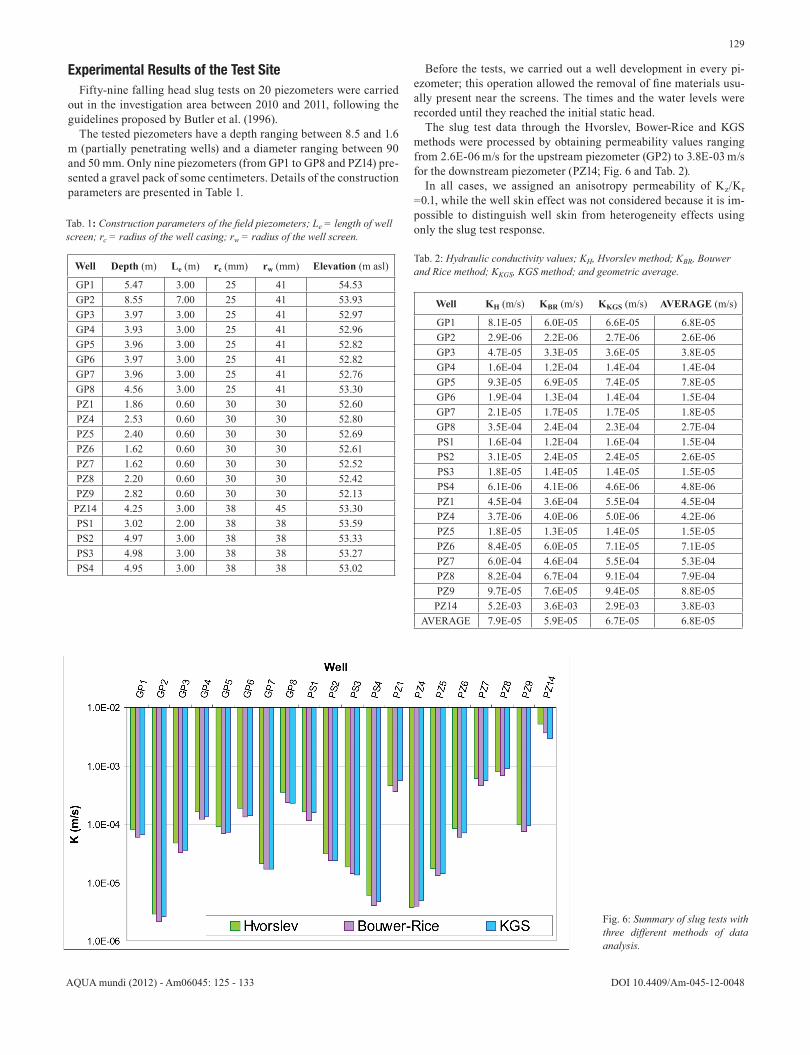
Tab. 1: Construction parameters of the field piezometers; Le = length of well screen; rc = radius of the well casing; rw = radius of the well screen.

Tab. 2: Hydraulic conductivity values; KH, Hvorslev method; KBR, Bouwer and Rice method; KKGS, KGS method; and geometric average.

Experimental Results of the Test SiteFifty-nine falling head slug tests on 20 piezometers were carried

out in the investigation area between 2010 and 2011, following the guidelines proposed by Butler et al. (1996).

The tested piezometers have a depth ranging between 8.5 and 1.6 m (partially penetrating wells) and a diameter ranging between 90 and 50 mm. Only nine piezometers (from GP1 to GP8 and PZ14) pre-sented a gravel pack of some centimeters. Details of the construction parameters are presented in Table 1.

Well Depth (m) Le (m) rc (mm) rw (mm) Elevation (m asl)

GP1 5.47 3.00 25 41 54.53GP2 8.55 7.00 25 41 53.93GP3 3.97 3.00 25 41 52.97GP4 3.93 3.00 25 41 52.96GP5 3.96 3.00 25 41 52.82GP6 3.97 3.00 25 41 52.82GP7 3.96 3.00 25 41 52.76GP8 4.56 3.00 25 41 53.30PZ1 1.86 0.60 30 30 52.60PZ4 2.53 0.60 30 30 52.80PZ5 2.40 0.60 30 30 52.69PZ6 1.62 0.60 30 30 52.61PZ7 1.62 0.60 30 30 52.52PZ8 2.20 0.60 30 30 52.42PZ9 2.82 0.60 30 30 52.13

PZ14 4.25 3.00 38 45 53.30PS1 3.02 2.00 38 38 53.59PS2 4.97 3.00 38 38 53.33PS3 4.98 3.00 38 38 53.27PS4 4.95 3.00 38 38 53.02

Before the tests, we carried out a well development in every pi-ezometer; this operation allowed the removal of fine materials usu-ally present near the screens. The times and the water levels were recorded until they reached the initial static head.

The slug test data through the Hvorslev, Bower-Rice and KGS methods were processed by obtaining permeability values ranging from 2.6E-06 m/s for the upstream piezometer (GP2) to 3.8E-03 m/s for the downstream piezometer (PZ14; Fig. 6 and Tab. 2).

In all cases, we assigned an anisotropy permeability of Kz/Kr =0.1, while the well skin effect was not considered because it is im-possible to distinguish well skin from heterogeneity effects using only the slug test response.

Well KH (m/s) KBR (m/s) KKGS (m/s) AVERAGE (m/s)

GP1 8.1E-05 6.0E-05 6.6E-05 6.8E-05GP2 2.9E-06 2.2E-06 2.7E-06 2.6E-06GP3 4.7E-05 3.3E-05 3.6E-05 3.8E-05GP4 1.6E-04 1.2E-04 1.4E-04 1.4E-04GP5 9.3E-05 6.9E-05 7.4E-05 7.8E-05GP6 1.9E-04 1.3E-04 1.4E-04 1.5E-04GP7 2.1E-05 1.7E-05 1.7E-05 1.8E-05GP8 3.5E-04 2.4E-04 2.3E-04 2.7E-04PS1 1.6E-04 1.2E-04 1.6E-04 1.5E-04PS2 3.1E-05 2.4E-05 2.4E-05 2.6E-05PS3 1.8E-05 1.4E-05 1.4E-05 1.5E-05PS4 6.1E-06 4.1E-06 4.6E-06 4.8E-06PZ1 4.5E-04 3.6E-04 5.5E-04 4.5E-04PZ4 3.7E-06 4.0E-06 5.0E-06 4.2E-06PZ5 1.8E-05 1.3E-05 1.4E-05 1.5E-05PZ6 8.4E-05 6.0E-05 7.1E-05 7.1E-05PZ7 6.0E-04 4.6E-04 5.5E-04 5.3E-04PZ8 8.2E-04 6.7E-04 9.1E-04 7.9E-04PZ9 9.7E-05 7.6E-05 9.4E-05 8.8E-05

PZ14 5.2E-03 3.6E-03 2.9E-03 3.8E-03AVERAGE 7.9E-05 5.9E-05 6.7E-05 6.8E-05

Fig. 6: Summary of slug tests with three different methods of data analysis.

130

DOI 10.4409/Am-045-12-0048 AQUA mundi (2012) - Am06045: 125 - 133

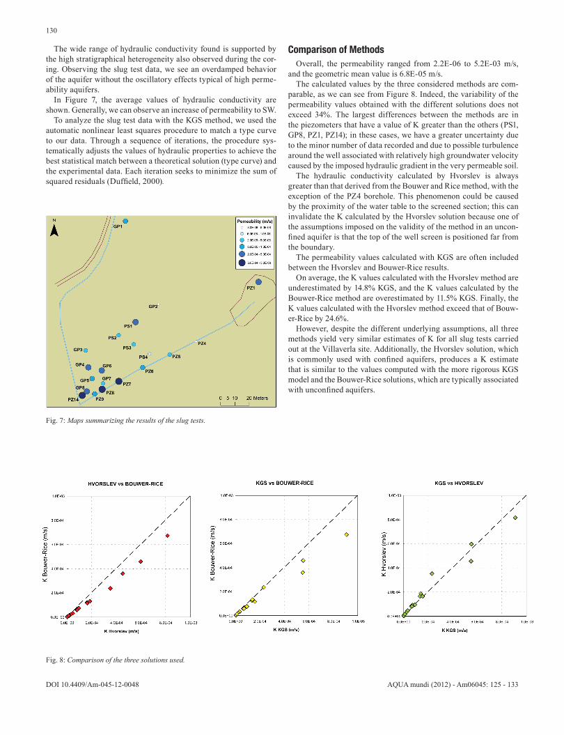
The wide range of hydraulic conductivity found is supported by the high stratigraphical heterogeneity also observed during the cor-ing. Observing the slug test data, we see an overdamped behavior of the aquifer without the oscillatory effects typical of high perme-ability aquifers.

In Figure 7, the average values of hydraulic conductivity are shown. Generally, we can observe an increase of permeability to SW.

To analyze the slug test data with the KGS method, we used the automatic nonlinear least squares procedure to match a type curve to our data. Through a sequence of iterations, the procedure sys-tematically adjusts the values of hydraulic properties to achieve the best statistical match between a theoretical solution (type curve) and the experimental data. Each iteration seeks to minimize the sum of squared residuals (Duffield, 2000).

Fig. 7: Maps summarizing the results of the slug tests.

Fig. 8: Comparison of the three solutions used.

Comparison of MethodsOverall, the permeability ranged from 2.2E-06 to 5.2E-03 m/s,

and the geometric mean value is 6.8E-05 m/s.The calculated values by the three considered methods are com-

parable, as we can see from Figure 8. Indeed, the variability of the permeability values obtained with the different solutions does not exceed 34%. The largest differences between the methods are in the piezometers that have a value of K greater than the others (PS1, GP8, PZ1, PZ14); in these cases, we have a greater uncertainty due to the minor number of data recorded and due to possible turbulence around the well associated with relatively high groundwater velocity caused by the imposed hydraulic gradient in the very permeable soil.

The hydraulic conductivity calculated by Hvorslev is always greater than that derived from the Bouwer and Rice method, with the exception of the PZ4 borehole. This phenomenon could be caused by the proximity of the water table to the screened section; this can invalidate the K calculated by the Hvorslev solution because one of the assumptions imposed on the validity of the method in an uncon-fined aquifer is that the top of the well screen is positioned far from the boundary.

The permeability values calculated with KGS are often included between the Hvorslev and Bouwer-Rice results.

On average, the K values calculated with the Hvorslev method are underestimated by 14.8% KGS, and the K values calculated by the Bouwer-Rice method are overestimated by 11.5% KGS. Finally, the K values calculated with the Hvorslev method exceed that of Bouw-er-Rice by 24.6%.

However, despite the different underlying assumptions, all three methods yield very similar estimates of K for all slug tests carried out at the Villaverla site. Additionally, the Hvorslev solution, which is commonly used with confined aquifers, produces a K estimate that is similar to the values computed with the more rigorous KGS model and the Bouwer-Rice solutions, which are typically associated with unconfined aquifers.

131

AQUA mundi (2012) - Am06045: 125 - 133 DOI 10.4409/Am-045-12-0048

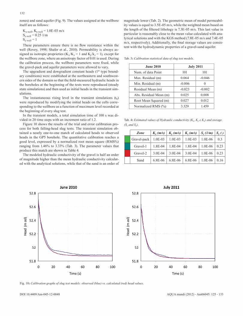
Fig. 9: Property zones of slug test models: A) plan view at layer 1 and B) SW-NE section at column 69.

Numerical Simulation of Slug TestsFinally, the results of some slug tests were simulated numerically

because the models offer an ideal tool to reproduce well-aquifer in-teraction and then to verify the results of analytical solutions. The numerical model was applied at the southwestern portion of the study site, where the subsoil is composed mainly of gravel and sand with less heterogeneity.

The results of two slug tests conducted in the GP5 borehole were analyzed using a three-dimensional finite difference groundwater flow model. The applied code was MODFLOW 2000, developed by the U.S. Geological Survey (Harbaugh et al., 2000), and is an up-dated version of the original MODFLOW (McDonald and Harbaugh, 1988). Rovey (1998) verified the ability of MODFLOW to reproduce wellbore tests with reasonable accuracy, although it is not possible to simulate radial symmetry flow around a line source with this code.

To analyze the slug test data, four simulations were implemented and calibrated. Two steady-state simulations reproduced the ground-water head distribution prior to the tests, and therefore, two tran-sient simulations reproduced the falling level during the slug tests performed in June 2010 and July 2011. The model domain is a 18 x 20 m rectangle centered on a GP5 borehole and oriented with an inclination of 50° from the north direction according to the mean groundwater flow direction (Fig. 9).

A high-spatial-resolution, non-uniform grid with cell dimensions ranging from 1 cm to 42 cm resulted in 140 columns (X-dimension) by 150 rows (Y-dimension). The minimum 1 cm horizontal grid spacing was designed to represent the nominal diameter of the GP5 borehole (2 in) and, separately, the 2-cm-thick gravel-pack sur-rounding the screen (Maher and Donovan, 1997; Shafer et al., 2010). The horizontal cell dimension expansion factor for telescoping cell widths to the model boundaries was 1.17, less than 1.5. Along ver-tical axes, 22 variables thickness layers were represented, starting from the topographical surface. Layers 1-13 represent the upper gravel, on average, from 52.38 m a.s.l. to 49.97 m a.s.l., and layers 13-22 correspond to lower sands, from the bottom of the gravels to 48.61 m a.s.l.

The vertical discretization was designed to break the screen inter-val into segments so that the model results would be directly compa-rable to the elevation of the pressure transducer in the well. In other words, the model setup was structured so that the simulation of the slug test was representative of the well configuration and the eleva-tion of the level probe.

Five zones were distinguished in the model domain: three of hy-draulic conductivity (Kx, Ky and Kz) and two of storage (Ss, specific storage and Sy, specific yield), which correspond, respectively to wellbore, gravel-pack surrounding the screen, gravel aquifer (two

132

DOI 10.4409/Am-045-12-0048 AQUA mundi (2012) - Am06045: 125 - 133

zones) and sand aquifer (Fig. 9). The values assigned at the wellbore itself are as follows:

Kx-well, Ky-well = 1.0E-03 m/sSs-well = 0.25 1/mSy-well = 1These parameters ensure there is no flow resistance within the

well (Rovey, 1998; Shafer et al., 2010). Permeability is always as-signed as isotropic proprieties (Kx/Kz = 1 and Ky/kz = 1), except for the wellbore zone, where an anisotropy factor of 0.01 is used. During the calibration process, the wellbore parameters were fixed, while the gravel-pack and aquifer parameters were allowed to vary.

The upgradient and dowgradient constant heads (1st type bound-ary conditions) were established at the northeastern and southwest-ern sides of the domain so that the field-measured hydraulic heads in the boreholes at the beginning of the tests were reproduced (steady state simulations) and then used as initial heads in the transient sim-ulations.

The instantaneous rising level in the transient simulations (t0) were reproduced by modifying the initial heads on the cells corre-sponding to the wellbore as a function of maximum level recorded at the beginning of every slug test.

In the transient models, a total simulation time of 100 s was di-vided in 20 time steps with an increment ratio of 1.2.

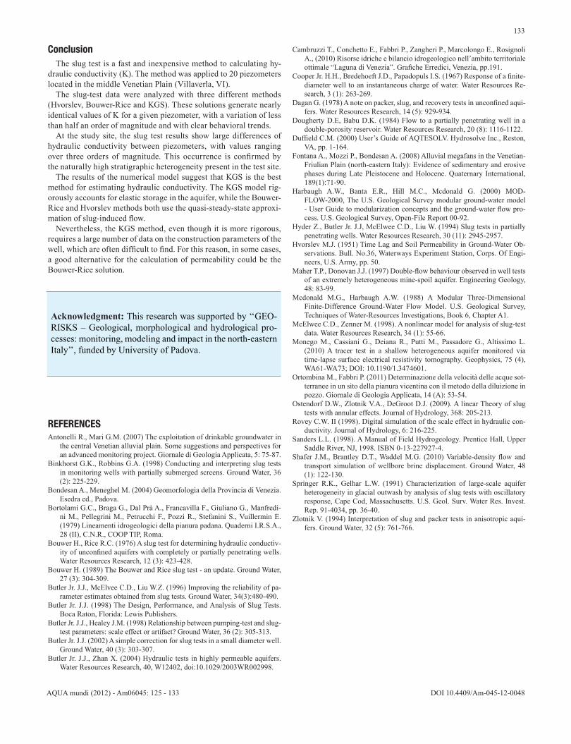
Figure 10 shows the results of the trial and error calibration pro-cess for both falling-head slug tests. The transient simulation ob-tained a nearly one-to-one match of calculated heads to observed heads in the GP5 borehole. The quantitative calibration reaches a good level, expressed by a normalized root mean square (RMS%) ranging from 1.46% to 3.33% (Tab. 3). The parameter values that produce this match are shown in Table 4.

The modeled hydraulic conductivity of the gravel is half an order of magnitude higher than the mean hydraulic conductivity calculat-ed with the analytical solutions, while that of the sand is an order of

Fig. 10: Calibration graphs of slug test models: observed (blue) vs. calculated (red) head values.

magnitude lower (Tab. 2). The geometric mean of model permeabil-ity values is equal to 3.5E-05 m/s, while the weighted mean based on the length of the filtered lithology is 7.3E-05 m/s. This last value in particular is reasonably close to the mean value calculated with ana-lytical solutions and with the KGS method (7.8E-05 m/s and 7.4E-05 m/s, respectively). Additionally, the final storage values are consis-tent with the hydrodynamic properties of a gravel-sand aquifer.

June 2010 July 2011Num. of data Point 101 101Max. Residual (m) 0.064 -0.046Min. Residual (m) -0.006 0Residual Mean (m) -0.023 -0.002Abs. Residual Mean (m) 0.025 0.008Root Mean Squared (m) 0.027 0.012Normalized RMS (%) 3.329 1.459

Tab. 3: Calibration statistical data of slug test models.

Tab. 4: Estimated values of Hydraulic conductivity (Kx, Ky e Kz) and storage (Ss and Sy).

Zone Kx (m/s) Ky (m/s) Kz (m/s) Ss (1/m) Sy ( )

Gravel-pack 1.0E-03 1.0E-03 1.0E-03 1.0E-06 0.3

Gravel-1 1.8E-04 1.8E-04 1.8E-04 1.0E-06 0.23

Gravel-2 3.0E-04 3.0E-04 3.0E-04 1.0E-06 0.23

Sand 6.8E-06 6.8E-06 6.8E-06 1.0E-06 0.16

133

AQUA mundi (2012) - Am06045: 125 - 133 DOI 10.4409/Am-045-12-0048

ConclusionThe slug test is a fast and inexpensive method to calculating hy-

draulic conductivity (K). The method was applied to 20 piezometers located in the middle Venetian Plain (Villaverla, VI).

The slug-test data were analyzed with three different methods (Hvorslev, Bouwer-Rice and KGS). These solutions generate nearly identical values of K for a given piezometer, with a variation of less than half an order of magnitude and with clear behavioral trends.

At the study site, the slug test results show large differences of hydraulic conductivity between piezometers, with values ranging over three orders of magnitude. This occurrence is confirmed by the naturally high stratigraphic heterogeneity present in the test site.

The results of the numerical model suggest that KGS is the best method for estimating hydraulic conductivity. The KGS model rig-orously accounts for elastic storage in the aquifer, while the Bouwer-Rice and Hvorslev methods both use the quasi-steady-state approxi-mation of slug-induced flow.

Nevertheless, the KGS method, even though it is more rigorous, requires a large number of data on the construction parameters of the well, which are often difficult to find. For this reason, in some cases, a good alternative for the calculation of permeability could be the Bouwer-Rice solution.

REFERENCESAntonelli R., Mari G.M. (2007) The exploitation of drinkable groundwater in

the central Venetian alluvial plain. Some suggestions and perspectives for an advanced monitoring project. Giornale di Geologia Applicata, 5: 75-87.

Binkhorst G.K., Robbins G.A. (1998) Conducting and interpreting slug tests in monitoring wells with partially submerged screens. Ground Water, 36 (2): 225-229.

Bondesan A., Meneghel M. (2004) Geomorfologia della Provincia di Venezia. Esedra ed., Padova.

Bortolami G.C., Braga G., Dal Prà A., Francavilla F., Giuliano G., Manfredi-ni M., Pellegrini M., Petrucchi F., Pozzi R., Stefanini S., Vuillermin E. (1979) Lineamenti idrogeologici della pianura padana. Quaderni I.R.S.A., 28 (II), C.N.R., COOP TIP, Roma.

Bouwer H., Rice R.C. (1976) A slug test for determining hydraulic conductiv-ity of unconfined aquifers with completely or partially penetrating wells. Water Resources Research, 12 (3): 423-428.

Bouwer H. (1989) The Bouwer and Rice slug test - an update. Ground Water, 27 (3): 304-309.

Butler Jr. J.J., McElvee C.D., Liu W.Z. (1996) Improving the reliability of pa-rameter estimates obtained from slug tests. Ground Water, 34(3):480-490.

Butler Jr. J.J. (1998) The Design, Performance, and Analysis of Slug Tests. Boca Raton, Florida: Lewis Publishers.

Butler Jr. J.J., Healey J.M. (1998) Relationship between pumping-test and slug-test parameters: scale effect or artifact? Ground Water, 36 (2): 305-313.

Butler Jr. J.J. (2002) A simple correction for slug tests in a small diameter well. Ground Water, 40 (3): 303-307.

Butler Jr. J.J., Zhan X. (2004) Hydraulic tests in highly permeable aquifers. Water Resources Research, 40, W12402, doi:10.1029/2003WR002998.

Cambruzzi T., Conchetto E., Fabbri P., Zangheri P., Marcolongo E., Rosignoli A., (2010) Risorse idriche e bilancio idrogeologico nell’ambito territoriale ottimale “Laguna di Venezia”. Grafiche Erredici, Venezia, pp.191.

Cooper Jr. H.H., Bredehoeft J.D., Papadopuls I.S. (1967) Response of a finite-diameter well to an instantaneous charge of water. Water Resources Re-search, 3 (1): 263-269.

Dagan G. (1978) A note on packer, slug, and recovery tests in unconfined aqui-fers. Water Resources Research, 14 (5): 929-934.

Dougherty D.E, Babu D.K. (1984) Flow to a partially penetrating well in a double-porosity reservoir. Water Resources Research, 20 (8): 1116-1122.

Duffield C.M. (2000) User’s Guide of AQTESOLV. Hydrosolve Inc., Reston, VA, pp. 1-164.

Fontana A., Mozzi P., Bondesan A. (2008) Alluvial megafans in the Venetian-Friulian Plain (north-eastern Italy): Evidence of sedimentary and erosive phases during Late Pleistocene and Holocene. Quaternary International, 189(1):71-90.

Harbaugh A.W., Banta E.R., Hill M.C., Mcdonald G. (2000) MOD-FLOW-2000, The U.S. Geological Survey modular ground-water model - User Guide to modularization concepts and the ground-water flow pro-cess. U.S. Geological Survey, Open-File Report 00-92.

Hyder Z., Butler Jr. J.J, McElwee C.D., Liu W. (1994) Slug tests in partially penetrating wells. Water Resources Research, 30 (11): 2945-2957.

Hvorslev M.J. (1951) Time Lag and Soil Permeability in Ground-Water Ob-servations. Bull. No.36, Waterways Experiment Station, Corps. Of Engi-neers, U.S. Army, pp. 50.

Maher T.P., Donovan J.J. (1997) Double-flow behaviour observed in well tests of an extremely heterogeneous mine-spoil aquifer. Engineering Geology, 48: 83-99.

Mcdonald M.G., Harbaugh A.W. (1988) A Modular Three-Dimensional Finite-Difference Ground-Water Flow Model. U.S. Geological Survey, Techniques of Water-Resources Investigations, Book 6, Chapter A1.

McElwee C.D., Zenner M. (1998). A nonlinear model for analysis of slug-test data. Water Resources Research, 34 (1): 55-66.

Monego M., Cassiani G., Deiana R., Putti M., Passadore G., Altissimo L. (2010) A tracer test in a shallow heterogeneous aquifer monitored via time-lapse surface electrical resistivity tomography. Geophysics, 75 (4), WA61-WA73; DOI: 10.1190/1.3474601.

Ortombina M., Fabbri P. (2011) Determinazione della velocità delle acque sot-terranee in un sito della pianura vicentina con il metodo della diluizione in pozzo. Giornale di Geologia Applicata, 14 (A): 53-54.

Ostendorf D.W., Zlotnik V.A., DeGroot D.J. (2009). A linear Theory of slug tests with annular effects. Journal of Hydrology, 368: 205-213.

Rovey C.W. II (1998). Digital simulation of the scale effect in hydraulic con-ductivity. Journal of Hydrology, 6: 216-225.

Sanders L.L. (1998). A Manual of Field Hydrogeology. Prentice Hall, Upper Saddle River, NJ, 1998. ISBN 0-13-227927-4.

Shafer J.M., Brantley D.T., Waddel M.G. (2010) Variable-density flow and transport simulation of wellbore brine displacement. Ground Water, 48 (1): 122-130.

Springer R.K., Gelhar L.W. (1991) Characterization of large-scale aquifer heterogeneity in glacial outwash by analysis of slug tests with oscillatory response, Cape Cod, Massachusetts. U.S. Geol. Surv. Water Res. Invest. Rep. 91-4034, pp. 36-40.

Zlotnik V. (1994) Interpretation of slug and packer tests in anisotropic aqui-fers. Ground Water, 32 (5): 761-766.

Acknowledgment: This research was supported by ‘‘GEO-RISKS – Geological, morphological and hydrological pro-cesses: monitoring, modeling and impact in the north-eastern Italy’’, funded by University of Padova.