Estimation of environmental exposure to ground-level ozone: an example of modelling for the Québec population

FOREWORD

The Québec government's Plan d’action 2006-2012 sur les changements climatiques (2006-2012 climate change action plan) entitled Le Québec et les changements climatiques, un défi pour l’avenir, involves several Québec government departments and organizations. Le Fonds vert, based on a charge on fuels and fossil fuels, provides most of the funding for 26 actions focusing on two major objectives: the reduction or avoidance of greenhouse gas emissions, and the adaptation to climate change.

The Ministère de la Santé et des Services sociaux (MSSS - ministry of health and social services) is responsible for the health component of Action 21 (a sustainable development action plan developed during the United Nations’ Rio Summit in 1992) targeting the implementation of mechanisms that will be used to prevent and attenuate the health impacts of climate change. It has therefore committed itself, to work in six action fields related to Québec's adaptation to climate change, each of which consists of several research or intervention projects.

This document presents approaches to model the geographic and temporal variation in ozone levels in order to better estimate the health risks represented by this pollutant. The work carried out in Québec contributes to the efforts deployed in public health surveillance and protection.

2

INTRODUCTION

Ozone (03) is a gas that is one of the normal components of the atmosphere. In the stratosphere, it forms the ozone layer and protects the earth from the sun's ultraviolet rays. However, in the troposphere, ozone does not provide this same protective effect; it is instead identified as being a greenhouse gas and one of the main components of smog. This gas could therefore constitute certain risks to human health.

The aim of this document is to present approaches to modelling the environmental exposure of populations to ground-level ozone, specifically the approaches carried out on Québec's population by the Chair on Air Pollution, Climate Change and Health at the Université de Montréal. The ultimate purpose of the work carried out in Québec is to better estimate the health risks represented by this pollutant, and to provide scientific knowledge to professionals and decision makers in public health to further protect Québec’s population.

Therefore, to briefly describe the context associated with the research work carried out in Québec, the first section presents the main characteristics of ozone as well as the conditions that favour its formation; the second section explains its short- and long-term health effects; and the third section addresses such things as ambient concentrations and the spatial and temporal distribution of ground-level ozone on Québec's territory.

Finally, the fourth section addresses more specifically the modelling of exposure, mainly by presenting the principal characteristics of different models for estimating exposure to ground-level ozone. The models presented are land use regression models as well as interpolation models, where the method is based on the proximity of the measuring stations, or kriging, or BME (Bayesian Maximum Entropy). This section ends with a short presentation of the objectives, methodology and a few results of the research work conducted in Québec.

In short, this study shows the success of the BME method developed by the Research Chair on Air Pollution, Climate Change and Health at the Université de Montréal. This method has the particular feature of making use of all of the network's data (just like kriging) as well as the data estimated by a land-use mixed regression model.

GENERAL CHARACTERISTICS OF OZONE

Ozone (03) is a colourless gas that constitutes one of the normal components of the atmosphere. In the stratosphere (or very high atmosphere), ozone forms and degrades continuously under the action of light rays and chemical reactions with products containing nitrogen, hydrogen or chlorine. This gas forms the ozone layer and protects the earth from overexposure to the sun's ultraviolet rays (Environment Canada, 2010a).

In the troposphere (or lower atmosphere, namely that breathed by humans), ozone does not have the same protective effect; it is identified as both a greenhouse gas and one of the primary components of smog. It presents certain human health risks (Environment Canada, 2010b).

Ground-level ozone is called a secondary pollutant because it is not emitted directly from a source; it is formed by photochemical reactions that occur on precursor pollutants such as nitrogen oxides (NOx), volatile organic compounds (VOCs), and carbon monoxide (CO).

3

These precursors are essentially of anthropic origin (meaning that they come from the combustion of gasoline and motor vehicle oils, from industrial emissions including those from electrical and coal-fired power plants, from the evaporation of liquid fuels and solvents, etc.); and, to a lesser extent, these precursors are of natural origin (i.e., they are generated by burning vegetation during forest fires, etc.) (Environment Canada, 2010b; Environment Canada, 2010c). The formation of ozone and its compounds is complex and depends on numerous factors such as the intensity and distribution of sun rays, the concentrations of precursor pollutants in the ambient air, as well as the rates of chemical reactions and other atmospheric processes (U.S. EPA, 2006). In general, the conditions for ozone formation are more favourable in the summer when the days are hot and sunny (MDDEP, 2010a) and the air mass is stable (anticyclone). Section 3, which deals with the environmental exposure of the Québec population, provides more details on these conditions and on the spatial and temporal distribution of ozone levels in Québec.

HEALTH EFFECTS OF GROUND-LEVEL OZONE

Studying the health effects of atmospheric pollutants is a delicate task because these effects generally have many causes (not belonging to a substance), and populations are often exposed to mixtures of pollutants (U.S. EPA, 2006; INSPQ, 2012). Identifying the toxic effects of a substance such as ozone therefore becomes difficult, and the conclusions drawn from these effects often come from the synthesis of scientific studies in many disciplines (toxicology, epidemiology, etc.).

From the toxicological standpoint, the main routes of ozone absorption and elimination are inhalation and exhalation, respectively. This gas, which is moderately soluble, can penetrate the lungs, reach the bronchioles and alveoli, and result in damage by directly oxidizing the molecules of the human body or even by forming free radicals or reactive intermediates in the lower respiratory tract (INRS, 1997; U.S. EPA, 2006).

Furthermore, epidemiological studies suggest that there is a relationship between short-term ozone exposure (one to a few days) and certain respiratory effects, including a reduction in pulmonary function and an increase in lung inflammation, pulmonary permeability, respiratory tract hyperreactivity, as well as emergency room visits and hospitalizations attributable to respiratory problems (U.S. EPA, 2006). A probable association is also suggested with mortality, and scientific knowledge also shows a possible association with cardiovascular and neurological effects (U.S. EPA, 2006).

As for long-term exposure, epidemiological evidence suggests a possible link between respiratory morbidities, such as the emergence of new cases of asthma, and an increase in respiratory symptoms in asthmatics (U.S. EPA, 2006). Studies also report a possible relationship to cardiovascular and neurological effects, toxic reproductive and developmental effects, as well as to combined all-cause mortality (U.S. EPA, 2006).

Thus, the effects of ozone exposure vary greatly. However, their extent could depend not only on different parameters associated with exposure such as concentration, duration, and co-exposure to other environmental factors (e.g., heat), but also on individual parameters, including the intensity of the physical exercise performed at the time of exposure or even individual susceptibilities (e.g., genetic predispositions, physical condition, age, sex). Children, asthmatics, and people working outdoors would be among those individuals most vulnerable to the effects of ozone (U.S. EPA, 2006).

4

ENVIRONMENTAL EXPOSURE OF THE QUÉBEC POPULATION

Sampling stations on Québec territory

In Québec, ambient ozone concentrations are recorded hourly by the Ministère du Développement durable, de l’Environnement, et de la Lutte contre les changements climatiques (MDDELCC - ministry of sustainable development, the environment, and the fight against climate change) through the programme de surveillance de la qualité de l’air (PSQA - air quality monitoring program). This program covers the territory where more than 95% of the Québec population lives (INSPQ, 2012). In 2007, only 46 ground-level ozone sampling stations were in operation.

The measuring stations are unequally distributed over the territory, meaning that they are present in larger numbers in the south of the province and at locations where the population density is greater. They are managed in collaboration with several partners, namely the City of Montréal, federal government departments, and industries (INSPQ, 2012). Other stations also exist, in numbers that vary over time, and that are operated in the context of special projects (MDDEP, 2010b). The locations of the air quality monitoring stations can be consulted on the Website of the MDDELCC (MDDEP, 2010b). Also, the majority of these stations can be seen online using the interactive maps of Environment Canada indicators (Environment Canada, 2012a).

Québec levels of risk management and international comparison

The relationship between ozone air pollution and health effects is of the linear type and without a safety threshold, which means that there is no ambient concentration below which the health risk is zero (U.S. EPA, 2006). As a result, no standard, no objective, no criterion—Québec or Canadian—is based on ozone's health effects.

However, for environmental risk management purposes, there is a Québec atmospheric quality standard of 80 parts per billion (ppb) for 1 hour of exposure. This standard generally applies to new projects or when installations that are already in operation are modified, but can also be used for depollution attestations required by the Environment Quality Act (MDDEFP, 2012).

For comparison purposes, the Canada-wide standard for air quality is 65 ppb—average for 3 consecutive years of the 4th highest annual value of 8-hour daily averages (CCME, 2000), and the United States Environmental Protection Agency (U.S. EPA) has proposed since 2008 a standard of 75 ppb for an 8-hour exposure (U.S. EPA, 2008). It should be noted that the American standard is currently being reviewed and could be lowered to 70 ppb for 8 hours (U.S. EPA, 2012). Finally, the World Health Organization (WHO) has had a guideline since 2005 of 100 µg/m3 (or approximately 50 ppb) as a daily average for 8 hours of exposure (WHO, 2006).

Ambient concentrations in Québec and comparison with Canada

For several years now, the province of Québec has been monitoring ambient ground-level ozone concentrations on its territory.

Between 1979 and 1994, Québec’s environment ministry (MDDEP, 1997) reported average annual hourly concentrations varying between 13 and 17 ppb and specified that there had been many periods when the hourly concentrations were above 80 ppb in the months of May through August. Between the months of April and September in the

5

years 2006 to 2008, the averages—calculated for the 3 consecutive years—of the highest 4 annual values of the daily averages for 8 hours varied between 58 and 68 ppb for the large agglomerations in Québec, namely Montréal, Québec City, Trois-Rivières, Sherbrooke, Saguenay, and Gatineau (MDDEP 2010a; MDDEP, 2010c). Finally, in a very recent report, Environment Canada (2012b) specified that between 1990 and 2009, the annual averages of the maximum daily concentrations over an 8-hour period, weighted according to the population and recorded at 25 monitoring stations spread out over all of southern Québec during the warm season (April to September) had varied between 31.81 (1993) and 41.47 (2001) ppb. In 2010, this average was 36.79 ppb, while it was 33.8, 43.1, 36.2, 30.3 and 38.2 ppb respectively for the Maritime Provinces, Southeastern Ontario, the Prairies and Northern Ontario, British Columbia, and all of Canada (Environment Canada, 2012b).

Spatial and temporal distribution of ozone levels in Québec

In Québec, ground-level ozone concentrations fluctuate considerably from one year to the next, and they are also very different in any given year. Ozone levels are high on hot days between the months of May and August and when an anticyclone (zone of high pressure) is present that moves slowly, that traps pollutants close to the ground, and that prevents them from dispersing and becoming diluted (Environment Canada, 1999).

Ground-level ozone concentrations also vary geographically on Québec's territory. The highest concentrations are generally found in the south of the province, due to the significant movements of air masses coming from the south and southwest. These air masses pass over the industrial and highly urbanized zones of the Great Lakes and Northeastern United States and shift the atmospheric pollutants (MDDEP, 1997; MDDEP, 2010a). Also, ozone concentrations are higher in rural environments than in urban or peri-urban environments. In fact, NOx, mainly produced by automobile traffic in urban environments, react very rapidly with ozone, and momentarily reduce its average concentrations in the ambient air. As a result, high ozone concentrations are likely to be found downwind from large urban agglomerations depending on the wind direction (MDDEP, 1997 and 2007).

ESTIMATION OF THE GROUND-LEVEL OZONE EXPOSURE OF POPULATIONS

Estimation of ozone-related health risks requires data on population exposure (Baker and Nieuwenhuijsen, 2009). For Québec, this exposure estimation is a complex task because the sampling stations are limited and unequally distributed over a large territory. Collecting individual measurements is a costly approach for estimating exposure (Jerret et al., 2005) and therefore cannot be carried out for the entire Québec population. To remedy this problem, which is a global problem, experts here and elsewhere have been developing, for several years now, spatiotemporal estimation methods for evaluating the ground-level ozone exposure of populations.

The traditional approach for estimating the exposure of individuals involves extrapolating to neighbouring environments the data recorded at sampling stations. For example, individuals are assigned the value of the station located closest to their place of residence. However, this method inevitably leads to incorrect classifications of exposure levels and tends to attenuate variations in individual exposure by incorrectly assigning the same concentrations to a large number of individuals (Bell, 2006; Vienneau et al., 2009; Beelen et al., 2009).

6

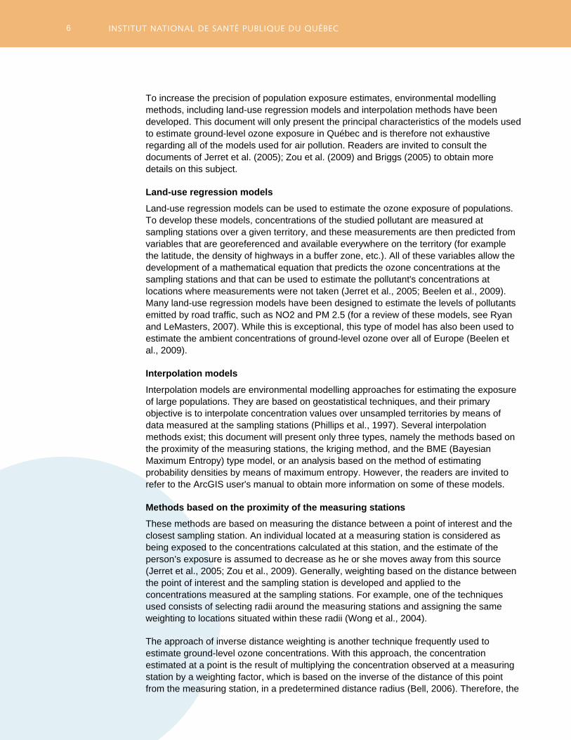
To increase the precision of population exposure estimates, environmental modelling methods, including land-use regression models and interpolation methods have been developed. This document will only present the principal characteristics of the models used to estimate ground-level ozone exposure in Québec and is therefore not exhaustive regarding all of the models used for air pollution. Readers are invited to consult the documents of Jerret et al. (2005); Zou et al. (2009) and Briggs (2005) to obtain more details on this subject.

Land-use regression models

Land-use regression models can be used to estimate the ozone exposure of populations. To develop these models, concentrations of the studied pollutant are measured at sampling stations over a given territory, and these measurements are then predicted from variables that are georeferenced and available everywhere on the territory (for example the latitude, the density of highways in a buffer zone, etc.). All of these variables allow the development of a mathematical equation that predicts the ozone concentrations at the sampling stations and that can be used to estimate the pollutant's concentrations at locations where measurements were not taken (Jerret et al., 2005; Beelen et al., 2009). Many land-use regression models have been designed to estimate the levels of pollutants emitted by road traffic, such as NO2 and PM 2.5 (for a review of these models, see Ryan and LeMasters, 2007). While this is exceptional, this type of model has also been used to estimate the ambient concentrations of ground-level ozone over all of Europe (Beelen et al., 2009).

Interpolation models

Interpolation models are environmental modelling approaches for estimating the exposure of large populations. They are based on geostatistical techniques, and their primary objective is to interpolate concentration values over unsampled territories by means of data measured at the sampling stations (Phillips et al., 1997). Several interpolation methods exist; this document will present only three types, namely the methods based on the proximity of the measuring stations, the kriging method, and the BME (Bayesian Maximum Entropy) type model, or an analysis based on the method of estimating probability densities by means of maximum entropy. However, the readers are invited to refer to the ArcGIS user's manual to obtain more information on some of these models.

Methods based on the proximity of the measuring stations

These methods are based on measuring the distance between a point of interest and the closest sampling station. An individual located at a measuring station is considered as being exposed to the concentrations calculated at this station, and the estimate of the person’s exposure is assumed to decrease as he or she moves away from this source (Jerret et al., 2005; Zou et al., 2009). Generally, weighting based on the distance between the point of interest and the sampling station is developed and applied to the concentrations measured at the sampling stations. For example, one of the techniques used consists of selecting radii around the measuring stations and assigning the same weighting to locations situated within these radii (Wong et al., 2004).

The approach of inverse distance weighting is another technique frequently used to estimate ground-level ozone concentrations. With this approach, the concentration estimated at a point is the result of multiplying the concentration observed at a measuring station by a weighting factor, which is based on the inverse of the distance of this point from the measuring station, in a predetermined distance radius (Bell, 2006). Therefore, the

7

concentration at a point of interest that is close to a measuring station will be estimated with a higher weighting factor than a point of interest located farther from a station.

For example, Bell (2006) measured the ozone concentrations in northeastern Georgia in the United States with ozone measurements at 8 sampling stations. In a 50-km radius around the measuring stations, the concentration was estimated using the following relationship: Wij=rij-3, where Wij was the weighting factor of the concentration at measuring station j for region i, and rij was the distance between measuring station j and the centroid of the county. Thus, the ozone concentration at a point was estimated by the average of the values for each of the measuring stations located in a 50-km radius from this point, to which were added a weighting factor as described by the above equation.

However, methods based on proximity of the stations, while often used for ozone estimation (Hopkins et al., 1999; Philips et al., 1997), have several limitations including the exclusion of all the parameters that affect the formation, destruction and dispersion of ozone (Zou et al., 2009). Also, these methods assume a specific relationship between the weighting factor and the distance, and this relationship is not always realistic or optimal (Philips et al., 1997). Often, the above-mentioned methods are used to do an exploratory analysis when estimating exposure (Jerret et al., 2005).

Kriging

Kriging, which is the most common interpolation method, also estimates the concentrations of a pollutant in a way similar to the method based on the proximity of the measuring stations, but uses a different weighting. In fact, instead of assuming a fixed weighting (such as the inverse of the distance, for example), this method estimates a weighting from the spatial and temporal covariance (dependence) that exists between all the concentrations measured at the sampling stations (Bell, 2006; Hopkins et al., 1999). Kriging makes it possible to define concentration-estimation equations over the entire area of study, which are ultimately used to produce maps representing a pollution area over all of the studied territory and for a given period (Jerret et al., 2005).

Several variants of kriging exist. Cokriging is of particular interest because it allows auxiliary variables to be considered in the analyses, such as population density, road traffic emissions, and meteorological conditions (Jerret et al., 2005), which are georeferenced over the entire territory. This method evaluates the mathematical relationship between the concentrations of the pollutant measured at the sampling stations and an auxiliary variable (or an index that represents the aggregation of several auxiliary variables on the territory), and then uses this mathematical relationship to interpolate and estimate the concentrations of the pollutant on the territory at the locations where no sampling station is located. Philips et al. (1997) used this method to estimate the ozone concentrations in the Southeastern United States. These authors developed an ozone exposure potential index, which was based on three variables (or factors) responsible for ozone formation and transport, namely 1) the average daily maximum temperature, 2) the wind direction, and 3) NOx emissions. To do this, they divided the studied territory into 20-km2 cells, and a value was determined for each of the following variables: temperature, wind direction, and NOx emissions. The values of these three variables were then multiplied in order to generate one index per cell, which expressed the relative potential of each of the cells to have a high ozone level. Finally, a mathematical relationship between these index values and the ozone concentrations measured at the sampling stations was determined, and the ozone concentrations at the locations where there was no sampling station were interpolated from this mathematical relationship. During this study, cokriging provided a

8

better prediction of the concentrations than the other interpolation methods (inverse distance weighting, kriging, etc.), which is furthermore generally the case when the auxiliary variables chosen are well correlated with the ozone concentrations measured at the sampling stations.

In brief, the success of these types of kriging is based on the fact that they take into consideration the dependence between the data for interpolating the pollutant's concentrations. They offer the best estimator from a linear model at any location whatsoever in the study area (Jerrett et al., 2005; Baker and Nieuwenhuijsen, 2009). However, these varieties of kriging also involve inherent constraints, such as the fact that they require a significant number of measuring stations to produce precise estimates (Yu et al., 2009). The interpolated pollution areas are often strongly biased and are almost invariably too regular due to a lack of representativity of the overall environment (Briggs, 2005; Jerret et al., 2005).

The BME (Bayesian Maximum Entropy) analysis method, or analysis based on the method of estimating the probability densities using maximum entropy

Another data interpolation method consists of a spatiotemporal analysis based on estimating the probability densities using the maximum entropy (BME). This technique makes it possible to increase the estimation by kriging. Just as with kriging, the BME estimates the weightings by means of measurement data originating from the sampling stations ("hard" data observed), but also uses data having various degrees of statistical uncertainty (or probability function) as predictions of mathematical models or measurements associated with a confidence interval ("soft" estimated data). All of this information (observed and estimated data) is shared in order to calculate a weighting that will be associated with each of the concentrations measured at the measuring stations closest to the point of interest to be estimated. This method provides an estimate of the exposure in terms of probability at all the points of interest in the study area and makes it possible to create maps representing pollution areas in a spatiotemporal continuum (Bogaert et al., 2009; De Nazelle et al., 2010).

Contrary to kriging and cokriging, the BME method does not have as many use constraints (Yu et al., 2009; Bogaert et al., 2009), and its interpolations integrate data with statistical uncertainties, which makes it a very interesting model for predicting concentrations of atmospheric pollutants (Kolovos et al., 2010; Christakos and Vyas, 1998; Christakos and Serre, 2000; Bogaert et al., 2009; De Nazelle et al., 2010). This method nevertheless requires significant knowledge of modelling, geostatistics and computer technology.

Research project for estimating the Québec population's ozone exposure

The dispersion of the sampling station network in Québec, the overrepresentation of certain metropolitan regions, and a lack of resources are the main reasons that motivate the use of environmental modelling for estimating the exposure of individuals in the population to ground-level ozone. This problem is addressed in a research project of the Research Chair on Air Pollution, Climate Change and Health at the Université de Montréal. The objective of this study is to compare three methods for estimating the exposure of Québec's population to summer ground-level ozone concentrations by means of the data from the network of sampling stations in the air quality monitoring program of the MDDELCC from 1990 to 2009.

 

9

The approaches that were developed for comparison purposes are: 1) a land-use mixed regression model that consists of several prediction variables including temperature, precipitation, the days of the year, the year, an estimate of the road traffic density, and the latitude; 2) a kriging interpolation model using all the network data; and 3) a BME-type model that uses all of the network data (as with kriging) as well as the data estimated by the land-use mixed regression model and its uncertainties. The estimates of these three approaches were compared by a cross validation that estimates and compares the prediction error of each of the models in relation to the real concentrations measured at the sampling stations.

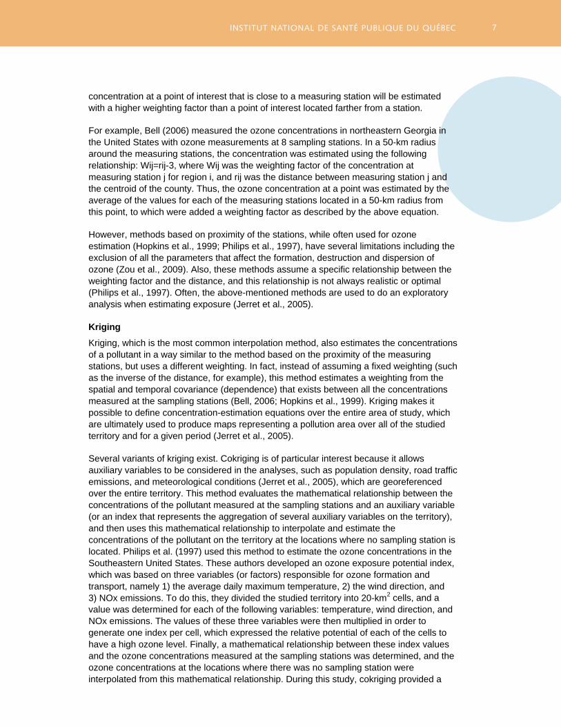
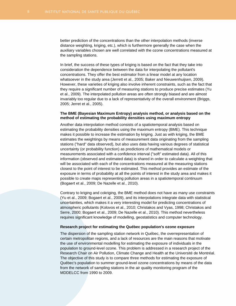
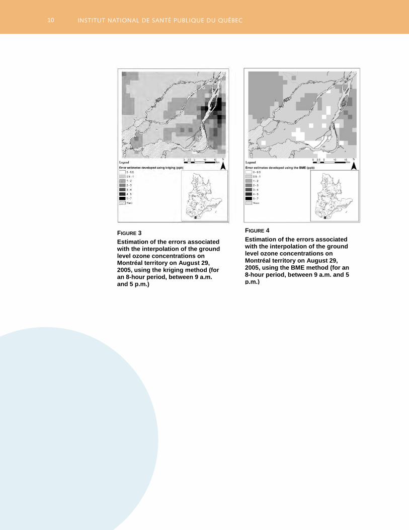
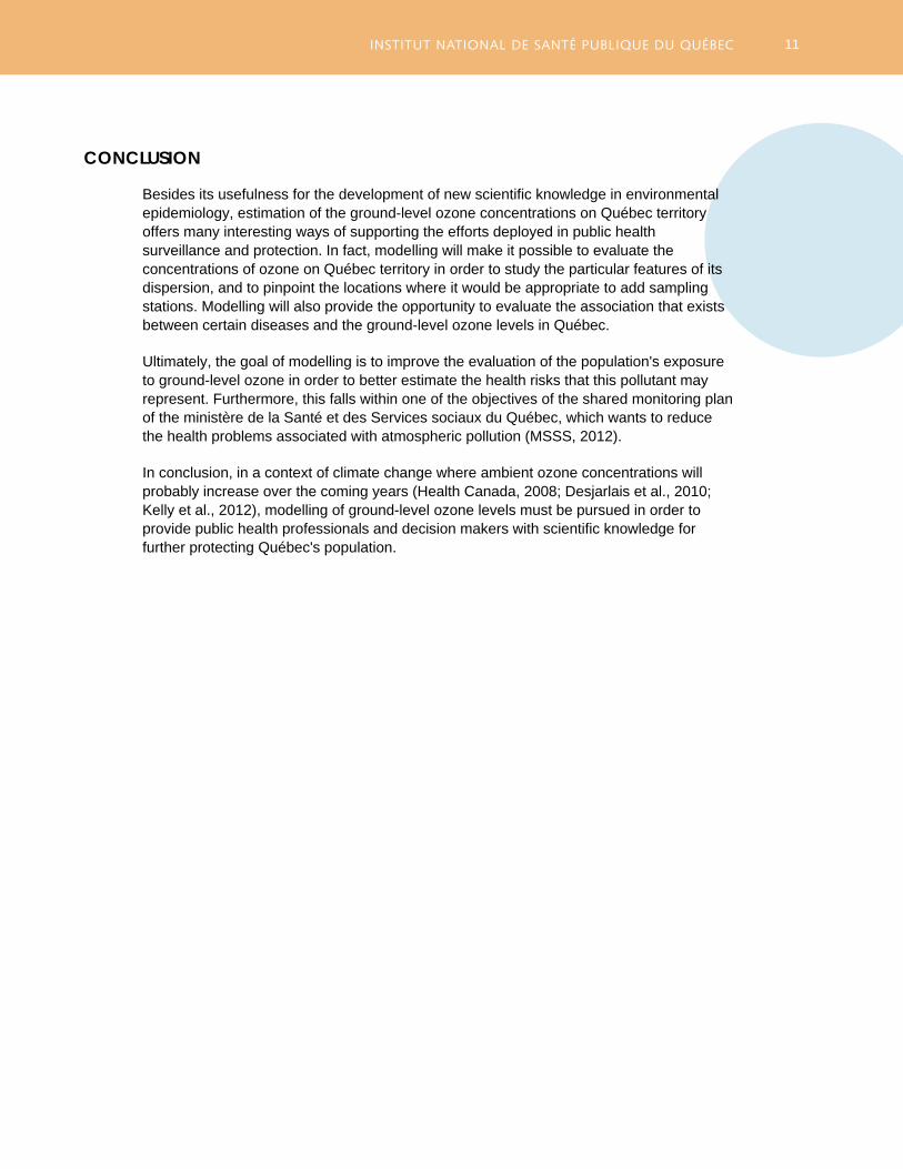
The results of this study suggest that the BME method can estimate the concentrations with a smaller error and with greater precision than the two other models (Adam-Poupart et al., 2014). The following figures present a few results of this study on the interpolation models (namely kriging and the BME method). Thus, Figures 1 and 2 illustrate the averages of the ozone concentrations in ppb (over 8 hours, from 9 a.m. to 5 p.m.) on Montréal territory on August 29, 2005, as they were estimated by kriging and the BME method, while Figures 3 and 4 show the estimates of the statistical errors associated with the averages of the estimated ozone concentrations. Comparison of Figures 1 and 2 indicates that the variations in the estimation of the concentrations produced by kriging are greater than those from the BME method for that day. However, the geographical dispersions are similar for the two interpolation models, showing mainly that the ozone concentrations are lower in eastern Montréal and higher in the southwest of the city. Furthermore, comparison of Figures 3 and 4 shows that kriging presents more statistical uncertainties for the averages of the estimated concentrations than the BME method. The results of the present study suggest that the BME method's success is associated with the integration of information from the land-use mixed regression model.

FIGURE 1

Estimation of the ground level ozone concentrations on Montréal territory on August 29, 2005, using the kriging method (for an 8-hour period, between 9 a.m. and 5 p.m.)

FIGURE 2

Estimation of the ground level ozone concentrations on Montréal territory on August 29, 2005, using the BME method (for an 8-hour period, between 9 a.m. and 5 p.m.) 

10

 

FIGURE 3

Estimation of the errors associated with the interpolation of the ground level ozone concentrations on Montréal territory on August 29, 2005, using the kriging method (for an 8-hour period, between 9 a.m. and 5 p.m.)

FIGURE 4

Estimation of the errors associated with the interpolation of the ground level ozone concentrations on Montréal territory on August 29, 2005, using the BME method (for an 8-hour period, between 9 a.m. and 5 p.m.)

11

CONCLUSION

Besides its usefulness for the development of new scientific knowledge in environmental epidemiology, estimation of the ground-level ozone concentrations on Québec territory offers many interesting ways of supporting the efforts deployed in public health surveillance and protection. In fact, modelling will make it possible to evaluate the concentrations of ozone on Québec territory in order to study the particular features of its dispersion, and to pinpoint the locations where it would be appropriate to add sampling stations. Modelling will also provide the opportunity to evaluate the association that exists between certain diseases and the ground-level ozone levels in Québec.

Ultimately, the goal of modelling is to improve the evaluation of the population's exposure to ground-level ozone in order to better estimate the health risks that this pollutant may represent. Furthermore, this falls within one of the objectives of the shared monitoring plan of the ministère de la Santé et des Services sociaux du Québec, which wants to reduce the health problems associated with atmospheric pollution (MSSS, 2012).

In conclusion, in a context of climate change where ambient ozone concentrations will probably increase over the coming years (Health Canada, 2008; Desjarlais et al., 2010; Kelly et al., 2012), modelling of ground-level ozone levels must be pursued in order to provide public health professionals and decision makers with scientific knowledge for further protecting Québec's population.

 

12

REFERENCES

Adam-Poupart, A., Brand, A., Fournier, M., Jerrett, M. and A. Smargiassi. (2014). Spatiotemporal Modeling of Ozone Levels in Quebec (Canada): A Comparison of Kriging, Land-Use Regression (LUR), and Combined Bayesian Maximum Entropy–LUR Approaches. Environmental Health Perspectives, vol. 122, No. 9, p. 970-976.

Baker, D. and Nieuwenhuijsen, M. J. (2009). Environmental epidemiology: study methods and application. United Kingdom: Oxford University Press.

Beelen, R., Hoek, G., et al. (2009). Mapping of background air pollution at fine spatial scale across the European Union. Science of the Total Environment, vol. 407, No. 6, p. 1852-1867.

Bell, M. L. (2006). The use of ambient air quality modeling to estimate individual and population exposure for human health research: a case study of ozone in the Northern Georgia Region of the United States. Environment International, vol. 32, No. 5, p. 586-593.

Bogaert, P., Christakos, G., et al. (2009). Spatiotemporal modelling of ozone distribution in the State of California. Atmospheric Environment, vol. 43, No. 15, p. 2471-2480.

Briggs, D. (2005). The role of Gis: coping with space (and time) in air pollution exposure assessment. Journal of Toxicology and Environmental Health, Part A, vol. 68 No. 13-14, p. 1243-1261.

Canadian Council of Ministers of the Environment – CCME. (2000). Canadian wide standards for particulate matter (PM) and ozone. [Online]. www.ccme.ca/assets/pdf/ pmozone_standard_e.pdf (Page consulted July 16, 2012).

Christakos, G. and Serre, M. L. (2000). BME analysis of spatiotemporal particulate matter distributions in North Carolina. Atmospheric Environment, vol. 34, No. 20, p. 3393-3406.

Christakos, G. and Vyas, V. M. (1998). A composite space/time approach to studying ozone distribution over eastern United States. Atmospheric Environment, vol. 32, No. 16, p. 2845-2857.

De Nazelle, A., Arunachalam, S., et al. (2010). Bayesian maximum entropy integration of ozone observations and model predictions: an application for attainment demonstration in North Carolina. Environmental Science and Technology, vol. 44, No. 15, 5707-5713.

Desjarlais, C., Blondlot, A., et al. (2010). Savoir s’adapter aux changements climatiques. Montréal : OURANOS. [Online]. http://www.ouranos.ca/fr/publications/documents/sscc_ francais_br-V22Dec2011_000.pdf (Page consulted June 2, 2012).

Environment Canada. (1999). National Ambient Air Quality Objectives For Ground-Level Ozone. The Federal/Provincial Working Group on Air Quality Objectives and Guidelines, Environment Canada.

Environment Canada (2010a). Ozone Layer. [Online]. http://www.ec.gc.ca/ozone/ default.asp?lang=En&n=DB5CBDE6-1 (Page consulted June 2, 2012).

Environment Canada (2010b). Ground Level Ozone. [Online]. http://www.ec.gc.ca/air/ default.asp?lang=En&n=590611CA-0 (Page consulted June 2, 2012).

Environment Canada. (2010c). Volatile Organic Compounds - Background. [Online]. http://www.ec.gc.ca/cov-voc/default.asp?lang=En&n=59828567-1 (Page consulted June 2, 2012).

Environment Canada. (2012a). Environmental Indicators -Interactive Indicator Maps. [Online]. URL: http://maps-cartes.ec.gc.ca/indicators-indicateurs/?mapId=1&xMin=-15853117.385229455&yMin=5011147.452426974&xMax=-4327636.512280503&yMax= 10881511.224726949&sr=102100. (Page consulted June 25, 2012).

13

Environment Canada. (2012b). Ambient Levels of Ozone. [Online]. http://www.ec.gc.ca/indicateurs-indicators/default.asp?lang=En&n=9EBBCA88-1. (Page consulted June 25, 2012).

Health Canada. (2008). Human Health in a Changing Climate: A Canadian Assessment of Vulnerabilities and Adaptive Capacity. Ottawa: Health Canada.Hopkins, L. P., Ensor, K. B. and Rifai, H. S. (1999). Empirical evaluation of ambient ozone interpolation procedures to support exposure models. Journal of the Air & Waste Management Association, vol. 49, No. 7, p. 839-846.

Institut national de santé publique du Québec – INSPQ. (2012). Bilan de la qualité de l’air au Québec en lien avec la santé, 1975-2009. Québec : Direction de la santé environnementale et de la toxicologie, Institut national de santé publique du Québec.

Institut national de recherche et de sécurité pour la prévention des accidents du travail et des maladies professionnelles – INRS (1997). Fiche toxicologique N.43 : Ozone. [Online]. http://www.inrs.fr/accueil/produits/bdd/doc/fichetox.html?refINRS=FT%2043. (Page consulted June 2, 2012).

Jerrett, M., Arain, A., et al. (2005). A review and evaluation of intraurban air pollution exposure models. Journal of Exposure Analysis and Environmental Epidemiology, vol. 15, No. 2, p. 185-204.

Kelly, J., Makar, P. A., et al. (2012). Projections of mid-century summer air-quality for North America: effects of changes in climate and precursor emissions. Atmospheric Chemistry and Physics, vol. 12, No. 2, p. 5367-5390.

Kolovos, A., Skupin, A., et al. (2010). Multi-perspective analysis and spatiotemporal mapping of air pollution monitoring data. Environmental Science and Technology, vol. 44, No. 17, p. 6738-6744.

Ministère du Développement durable, de l’Environnement et des Parcs – MDDEP. (1997). La qualité de l’air au Québec, de 1975 à 1994. Québec: Ministère du Développement durable, de l’Environnement et des Parcs, Direction du milieu atmosphérique et Service de la qualité de l’atmosphère. Québec.

Ministère du Développement durable, de l’Environnement et des Parcs – MDDEP. (2007). Formation and origin of smog. Info-Smog. [Online]. http://www.mddep.gouv.qc.ca/air/info-smog/fiche-formation_en.pdf (Page consulted July 1, 2012).

Ministère du Développement durable, de l’Environnement et des Parcs – MDDEP. (2010a). Fine particles and ozone in Quebec relative to the Canada-Wide standards (2009 Report). Québec: Ministère du Développement durable, de l’Environnement et des Parcs, Direction des politiques de la qualité de l’atmosphère.

Ministère du Développement durable, de l’Environnement et des Parcs – MDDEP. (2010b). Le programme de surveillance de la qualité de l’air. [Online]. http://www.mddefp.gouv.qc.ca/air/programme_surveillance/index.htm. (Page consulted June 2, 2012).

Ministère du Développement durable, de l’Environnement et des Parcs – MDDEP. (2010c). Mise à jour des critères québécois de qualité de l’air. Québec : Ministère du Développement durable, de l’Environnement et des Parcs, Direction du suivi de l’état de l’environnement.

Ministère du Développement durable, de l’Environnement de la Faune et des Parcs – MDDEFP. (2012). Regulation respecting the quality of the atmosphere: Environment Quality Act (R.S.Q., c. Q-2, a. 20, 31, 53, 70, 71, 72, 87 and 124.1).

Ministère de la Santé et des Services sociaux – MSSS. (2012). Santé environnementale-surveillance. [Online]. www.msss.gouv.qc.ca/sujets/santepub/environnement/index.php? surveillance. (Page consulted June 2, 2012).

14

Phillips, D. L., Lee, E. H., et al. (1997). Use of auxiliary data for spatial interpolation of ozone exposure in southeastern forests, Environmetrics, vol. 8, p. 43-61.

Ryan, P. H. and Lemasters, G.K. (2007). A review of land-use regression models for characterizing intraurban air pollution exposure. Inhalation Toxicology, vol. 19, suppl. 1, 127-133.

United State Environmental Protection Agency – U.S. EPA. (2006). Air quality criteria for ozone and other photochemical oxidants, No. EPA /600/P-93/004aF.

United States Environmental Protection Agency – U.S. EPA. (2008). National ambient air quality standards for ozone; final rule. [Online]. www.gpo.gov/fdsys/pkg/FR-2008-03-27/ html/E8-5645.htm (Page consulted July 16, 2012).

United States Environmental Protection Agency – U.S. EPA. (2012). Ground-level ozone-regulatory actions. [Online]. www.epa.gov/groundlevelozone/actions.html. (Page consulted July 16, 2012).

Vienneau, D., De Hoogh, K., et al. (2009). A GIS-based method for modelling air pollution exposures across Europe. Science of the Total Environment, vol. 408, No. 2, p. 255-266.

Wong, D. W., Yuan, L., et al. (2004). Comparison of spatial interpolation methods for the estimation of air quality data. Journal of Exposure Analysis and Environmental Epidemiology, vol. 14, No. 5, p. 404-415.

World Health Organization – WHO. (2006). WHO Air quality guidelines for particulate matter, ozone, nitrogen dioxide and sulfur dioxide. [Online]. http://whqlibdoc.who.int/hq/ 2006/WHO_SDE_PHE_OEH_06.02_eng.pdf. (Page consulted June 2, 2012).

Yu, H. L., Chen, J. C., et al. (2009). BME Estimation of residential exposure to ambient PM10 and ozone at multiple time scale. Environmental Health Perspectives, vol. 117, No. 4, p. 537-544.

Zou, B., Wilson, J. G., et al. (2009). Air pollution exposure assessment methods utilized in epidemiological studies. Journal of Environmental Monitoring, vol. 11, No. 3, p. 475-490.

 

AUTHORS

Ariane Adam-Poupart Department of environmental and occupational health Faculty of Medicine, Université de Montréal

Allan Brand Direction de la santé environnementale et de la toxicologie Institut national de santé publique du Québec

Michel Fournier Agence de la santé et des services sociaux de Montréal/Direction de santé publique

Audrey Smargiassi Direction de la santé environnementale et de la toxicologie Institut national de santé publique du Québec Research chair on air pollution, climate change and health, Faculty of Medicine, Université de Montréal

This study was funded by the Fonds vert in the context of Action 21 of the Plan d’action 2006-2012 sur les changements climatiques du gouvernement québécois.

TRANSLATION

The translation of this publication was made possible with funding from the Public Health Agency of Canada. The translation was done by Helen Fleischauer.

This document is available in its entirety in electronic format (PDF) on the Institut national de santé publique du Québec Web site at: http://www.inspq.qc.ca.

Reproductions for private study or research purposes are authorized by virtue of Article 29 of the Copyright Act. Any other use must be authorized by the Government of Québec, which holds the exclusive intellectual property rights for this document. Authorization may be obtained by submitting a request to the central clearing house of the Service de la gestion des droits d’auteur of Les Publications du Québec, using the online form at http://www.droitauteur.gouv.qc.ca/en/autorisation.php or by sending an e-mail to droit.auteur@cspq.gouv.qc.ca.

Information contained in the document may be cited provided that the source is mentioned.

LEGAL DEPOSIT – 1ST QUARTER 2015

BIBLIOTHÈQUE ET ARCHIVES NATIONALES DU QUÉBEC LIBRARY AND ARCHIVES CANADA ISBN: 978-2-550-68443-5 (FRENCH PDF) ISBN: 978-2-550-72535-0 (PDF)

©Gouvernement du Québec (2015)

Publication N°: 1954

Funding partner: