Estimation of Dynamic Models of Panel Data with … of Dynamic Models of Panel Data with...
59
Estimation of Dynamic Models of Panel Data with Cross-Sectional Dependence Valentin Verdier * October 14, 2013 Abstract This paper considers the estimation of dynamic panel data models when data are suspected to exhibit cross-sectional dependence. A new estimator is defined that makes use of cross-sectional dependence for estimation while being robust to its misspecification. It is shown that using cross-sectional dependence for estimation is important to obtain an estimator that is more accurate. The proposed estimator uses nuisance parameters parsimoniously so that it retains good small sample properties even if the number of available moment conditions is large. The estimation of the effect of attending private school on student achievement using a value added model is considered as an empirical application. Keywords: Panel Data, Dynamic Models, Cross-Sectional Dependence, Optimal Instru- ments * Department of Economics, Michigan State University, East Lansing, MI 48824, United States. Tel.: +1 5178810834. E-mail address: [email protected]. 1
Transcript of Estimation of Dynamic Models of Panel Data with … of Dynamic Models of Panel Data with...

Estimation of Dynamic Models of Panel Data with
Cross-Sectional Dependence
Valentin Verdier!
October 14, 2013
Abstract
This paper considers the estimation of dynamic panel data models when data are
suspected to exhibit cross-sectional dependence. A new estimator is defined that makes
use of cross-sectional dependence for estimation while being robust to its misspecification.
It is shown that using cross-sectional dependence for estimation is important to obtain
an estimator that is more accurate. The proposed estimator uses nuisance parameters
parsimoniously so that it retains good small sample properties even if the number of
available moment conditions is large. The estimation of the e!ect of attending private
school on student achievement using a value added model is considered as an empirical
application.
Keywords: Panel Data, Dynamic Models, Cross-Sectional Dependence, Optimal Instru-
ments
!Department of Economics, Michigan State University, East Lansing, MI 48824, United States. Tel.: +15178810834. E-mail address: [email protected].
1

1 Introduction
In the context of cross-sectionally independent panel data, an Instrumental Variable estimator
of linear dynamic models that is consistent under the assumption of mean independence of
transitory shocks can be found in early work by Anderson and Hsiao (1981). This estimator
uses first di!erencing, so that it is not a!ected by the presence of additive unobserved het-
erogeneity, and uses second lags of the dependent variable as instruments for the di!erenced
equations. In order to construct more e"cient estimators, Arellano and Bond (1991) proposed
using a GMM estimator (henceforth called the AB estimator) where all past outcomes with
lags of two or higher are used as instruments for the di!erenced equations at each time period.
When the dependent variable is very persistent over time, the AB estimator or the estimator
of Anderson and Hsiao (1981) are inaccurate because second and higher lags of the dependent
variable are weak instruments. To address this problem, papers such as Ahn and Schmidt
(1995), Arellano and Bover (1995), and Blundell and Bond (1998) considered using additional
moment conditions such as homoscedasticity, uncorrelation of the transitory shocks, or re-
strictions on initial conditions, in addition to the moment conditions used in Arellano and
Bond (1991). The resulting estimators are more accurate if these moment conditions hold
but inconsistent otherwise. Another approach to obtain e"ciency gains by using additional
assumptions can be found in the literature on First Di!erence Quasi-Maximum Likelihood
estimation, as in Hsiao et al. (2002) for instance which proposes an estimator based on few
nuisance parameters but that is not robust to heteroscedasticity or serial correlation of the
transitory shocks.
In this paper we will show that when cross-sectional dependence is present in panel data,
it can be used to construct stronger instruments so that significant e"ciency gains can be
achieved when estimating linear dynamic models without imposing any additional restriction.
We show that these e"ciency gains come mainly from using cross-sectional dependence to
obtain better predictors of one’s level of unobserved heterogeneity. The estimators we pro-
pose here are e"cient under some auxiliary restrictions but consistent as long as transitory
disturbances are mean independent of previous outcomes, i.e. our estimators are robust to
2

the auxiliary restrictions being violated.
In order to obtain an estimator that is e"cient under some auxiliary assumptions, we
model optimal instruments for dynamic models of panel data with cross-sectional dependence.
Optimal instruments are instruments that, once interacted with corresponding moment func-
tions, provide an optimal set of exactly identifying moment conditions so that the resulting
estimator achieves the asymptotic e"ciency bound for estimating unknown parameters from
the assumption of mean independence of the transitory shocks. Optimal instruments for es-
timating dynamic panel data models without cross-sectional dependence have been found in
Chamberlain (1992) and they can be generalized to the case of cross-sectional dependence. In
this paper, we propose auxiliary assumptions su"cient to model optimal instruments para-
metrically. The advantage of such an approach is that it makes use of few nuisance parameters
while providing a systematic way of computing weights for all available moment conditions.
Because our estimator uses few nuisance parameters, it exhibits good small sample properties.
We show that existing GMM estimators, such as the AB estimator, rely on the use of many
nuisance parameters to estimate weights for each of many moment conditions, which causes
small sample biases for these estimators and their standard errors when T is somewhat large,
as studied in Alvarez and Arellano (2003) or Windmeijer (2005) for the case of cross-sectional
independence. Arellano (2003) and Alvarez and Arellano (2004) have previously considered
modeling optimal instruments for dynamic panel data models in the special case of cross-
sectional independence. We will show that cross-sectional dependence can be particularly
useful to obtain more accurate estimators.
Previous work that has used dynamic models to analyze panel data has either ignored
cross-sectional correlation or has not made use of it to obtain stronger instruments. Mutl
(2006), for instance, studies a GMM estimator based on the same moment conditions as in
Anderson and Hsiao (1981) or Arellano and Bond (1991) and only uses an optimal weighting
matrix based on a specific model of spatial dependence. Elhorst (2005) and Su and Yang
(2013) generalize maximum likelihood estimators as in Hsiao et al. (2002) to the case of cross-
sectional dependence but these estimators are not robust to temporal heteroscedasticity, serial
3
correlation of the transitory shocks or misspecification of the cross-sectional dependence.
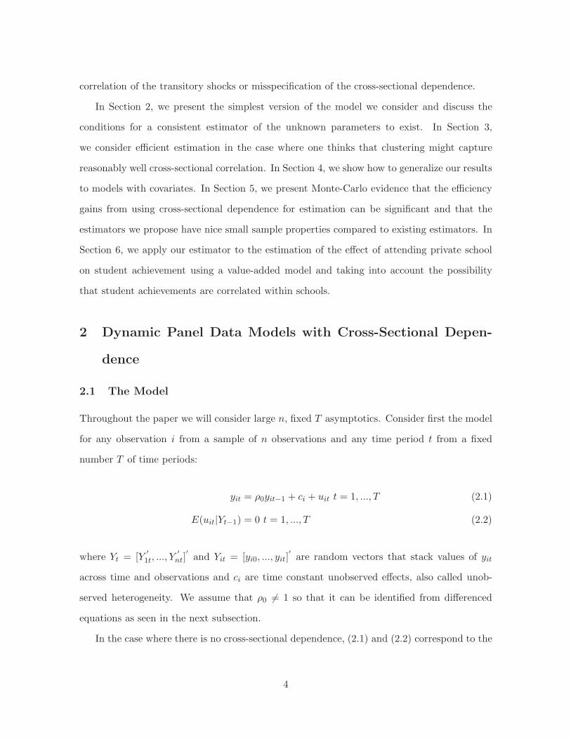
In Section 2, we present the simplest version of the model we consider and discuss the
conditions for a consistent estimator of the unknown parameters to exist. In Section 3,
we consider e"cient estimation in the case where one thinks that clustering might capture
reasonably well cross-sectional correlation. In Section 4, we show how to generalize our results
to models with covariates. In Section 5, we present Monte-Carlo evidence that the e"ciency
gains from using cross-sectional dependence for estimation can be significant and that the
estimators we propose have nice small sample properties compared to existing estimators. In
Section 6, we apply our estimator to the estimation of the e!ect of attending private school
on student achievement using a value-added model and taking into account the possibility
that student achievements are correlated within schools.
2 Dynamic Panel Data Models with Cross-Sectional Depen-
dence
2.1 The Model
Throughout the paper we will consider large n, fixed T asymptotics. Consider first the model
for any observation i from a sample of n observations and any time period t from a fixed
number T of time periods:
yit = !0yit"1 + ci + uit t = 1, ..., T (2.1)
E(uit|Yt"1) = 0 t = 1, ..., T (2.2)
where Yt = [Y"
1t, ..., Y"
nt]"
and Yit = [yi0, ..., yit]"
are random vectors that stack values of yit
across time and observations and ci are time constant unobserved e!ects, also called unob-
served heterogeneity. We assume that !0 != 1 so that it can be identified from di!erenced
equations as seen in the next subsection.
In the case where there is no cross-sectional dependence, (2.1) and (2.2) correspond to the
4

linear dynamic model for panel data as presented in Arellano and Bond (1991) for instance.
When there is cross-sectional dependence, (2.1) and (2.2) impose the restriction that cross-
sectional dependence does not cause Yt"1 to be endogenous.
For instance if contemporaneous spatial lags were omitted variables in (2.1), then (2.2)
would be violated. Some papers such as Cizek et al. (2011), Elhorst (2005), Su and Yang
(2013) and Baltagi et al. (2013) have considered models with both dynamic e!ects and con-
temporaneous spatial lag e!ects. Since estimators for such models rely on correct specification
of the form of cross-sectional dependence, we do not consider them here and concentrate on
models where arbitrary cross-sectional dependence is present in the residuals.1 However,
lagged values of the dependent variable of neigboring observations could also be included in
the model as covariates. We will discuss models with covariates in Section 4.
The objective of the next section is to characterize estimators for !0 that are consistent
when (2.1) and (2.2) hold under general conditions on the form of cross-sectional dependence
in ci and uit.
2.2 Consistent Estimation
The presence of unobserved heterogeneity rules out estimation of !0 by a regression and
because (2.1) and (2.2) form a dynamic model, Fixed E!ects estimation is also ruled out
because explanatory variables are not strictly exogenous.
To estimate !0, we will consider a first di!erence transformation. All of the derivations in
this paper can be generalized to other transformations, such as the forward filtering transfor-
mation presented in Arellano and Bover (1995) for instance, which can be useful in the case
of unbalanced panels. Define:
mit(!) = #yit " !#yit"1 # t = 2, ..., T (2.3)
1It is also important to note that, with cross-sectional dependence, it is not likely for E(uit|Yit#1) = 0 tohold without (2.2) holding. For instance suppose for simplicity that n = 2 and E(u1t|Yt#1) = !+ "1y1t#1 +"2y2t#1 != 0 so that "1 != 0 or "2 != 0. Then E(u1t|Y1t#1) = ! + "1y1t#1 + "2E(y2t#1|Y1t#1) and it likelythat E(y2t#1|Y1t#1) be a function of y10, ..., y1t#2 in addition to y1t#1 so that, in general, ! + "1y1t#1 !=""2E(y2t#1|Y1t#1) and E(u1t|y1t#1) != 0.
5

so that mit(!0) = uit " uit"1. Therefore (2.1) and (2.2) imply:
E(mit(!0)|Yt"2) = 0 # t = 2, ..., T (2.4)
Define mi(!) = [mit(!)]t=2,...,T . Sometimes we will also shorten notation by writing mi =
mi(!0), mit = mit(!0),!mi!" = !mi("0)
!" and !mit!" = !mit("0)
!" . Note that !mit!" = #yit"1 but it is
sometimes convenient to write !mit!" or !mi
!" .
Define:
Zi = [Zi2, ..., ZiT ] (2.5)
to be a matrix containing instruments for each time period so that Zit is a function of Yt"2
and therefore E(Zitmit(!0)) = 0 and E(Zimi(!0)) =!T
t=1 E(Zitmit(!0)) = 0.2
Define $ to be some weighting matrix. Define ! an estimator for !0 as:
! = argmin"(n"
i=1
Zimi(!))"
$n"
i=1
Zimi(!) (2.6)
Consider first the case where spatial dependence is captured by a large group of clusters
with fixed numbers of observations so that observations within a cluster might be related but
observations across clusters are independent. Standard results on asymptotic properties of
GMM estimators with clustering, found in White (2001) for instance, imply that ! will be
consistent for !0 and asymptotically normal as the number of clusters grows unboundedly
under usual regularity conditions.
For more general forms of cross-sectional dependence, Conley (1999), Jenish and Prucha
(2009), Jenish and Prucha (2012), and Kuersteiner and Prucha (2013) consider di!erent sets
of regularity conditions that guarantee that ! is consistent and asymptotically normal as long
as E(Zimi(!0)) = 0.
Therefore in this paper we will assume that either set of regularity conditions holds so
2Note that we need to assume #0 != 1 for E(Zimi(#)) = 0 to hold for # = #0 only since if #0 = 1 thenE(Zimi(#)) = 0 # #.
6

that as n $ %:3
&n(!" !0)
d$ N(0, V ) (2.7)
where:
V = (D"
$D)"1D"
$%$D(D"
$D)"1
D = plim(1
n
n"
i=1
Zi"mi
"!)
% = plim1
n
n"
i=1
n"
j=1
Zimim"
iZ"
i
In the next sections we consider e"cient feasible GMM estimation where the matrix of
instruments Zi and an estimator of the weighting matrix $ are chosen so that the resulting
estimator of !0 is e"cient under some auxiliary assumptions. It is important to note that
all of the estimators we propose will be asymptotically equivalent to estimators of the type
defined by (2.6) so that they will be consistent as long as (2.1) and (2.2) hold, independently
of whether the auxiliary models we specify are true or not.
3 E!cient Estimation under Clustering
In this section, we consider an auxiliary model for deriving optimal instruments that assumes
that every observation belongs to one of a large number of clusters. Observations are treated as
correlated within clusters but independent across clusters. While clustering only represents
a specific form of cross-sectional dependence, it might be a good approximation for more
general forms of dependence in many applications. In addition, the method outlined in this
section for the special case of clustering can easily be extended to other forms of cross-sectional
dependence. Therefore we restrict out attention in this paper to auxiliary models that make
use of the clustering assumption.
For simplicity we will consider in this section the case where each observation belongs to
3Note that in the case of clustering we consider {ng}g=1,...,G to be a set of fixed values, where ng denotesthe number of observations in cluster g and G the number of clusters. Then
$n-asymptotic normality or$
G-asymptotic normality are equivalent since n/min{ng} % G % n/max{ng}.
7

the same cluster across all time periods but the results in this section can be generalized to
clusters changing over time as shown in Section 6. Previous work that estimated dynamic
models of panel data with clustered sampling generally used estimators developed for i.i.d.
data such as the ones found in Anderson and Hsiao (1981), Arellano and Bond (1991), or
Ahn and Schmidt (1995), and adjusted inference by using clustered standard errors. Such an
analysis can be found for instance in de Brauw and Giles (2008) where farming households
are treated as clustered by village or Andrabi et al. (2011) where students are clustered
by school4. Topalova and Khandelwal (2010) and Balasubramanian and Sivadasan (2010)
consider the case where firms are clustered by industry.
In this section, we show that there is much to gain in terms of e"ciency by using a di!erent
estimator that takes into account correlation within cluster but is robust to misspecification
of the form of this correlation. We will consider the case where the data is composed of a
large number of clusters indexed by g = 1, ..., G, each with a fixed number of observations
denoted ng so that asymptotics will be performed for G $ %.
In the first subsection, we present the special case of two time periods since in this case
the problem reduces to estimating !0 from only one di!erenced equation using instrumental
variables.
3.1 Special Case of Independent Disturbances and T = 2
For this simple special case, we derive an e"cient estimator for the case where {uit}i=1,...,n,t=1,2
are independent both cross-sectionally and across time, where T = 2 and where we have
conditional homoscedasticity so that:
V ar(uit|Yt"1) = #2u # t = 1, 2 (3.1)
4We will show in Section 6 however that the clustering used in Andrabi et al. (2011) is not appropriate toobtain robust standard errors due to observations moving across clusters during the period of observation. Wewill show robust standard errors that take this factor into consideration.
8

When T = 2, there is only one di!erenced equation that can be used for estimation:
#yi2 = !0#yi1 +#ui2 (3.2)
for which the available instruments are Y0. Under the assumption of independence of distur-
bances and homoscedasticity, #ui2 is also cross-sectionally independent and homoscedastic,
so the optimal instrument for the di!erenced equation is the best prediction of #yi1 based on
all the available instruments, i.e. E(#yi1|Y0).
To find E(#yi1|Y0), note that under (2.1) and (2.2), yi1 = !0yi0 + ci + ui1 so that
E(#yi1|Y0) = (!0 " 1)yi0 +E(ci|Y0). Therefore the quality of the prediction of #yi1 based on
the instruments will depend on the quality of the prediction of ci based on the instruments.
In many applications, it is very likely that agents that belong to the same cluster will have
levels of unobserved heterogeneity that are related. For instance, farmers that live in the same
village might farm soils with similar qualities or develop similar farming practices. Firms that
operate in the same industry might also face similar constraints such as for instance regula-
tion or access to skilled labor force. Similarly, households that live in the same district might
have been selected based on common characteristics such as wealth, income, family status
or values. Therefore, in many applications, we can expect that using information from other
observations in the same cluster in addition to one’s own previous outcomes can provide a
better predictor for one’s level of unobserved heterogeneity.
For this simple case, we can derive an optimal predictor for ci by using the assumption
that for any observation i belonging to cluster g we have:
ci = cg + ei (3.3)
where {cg}g=1,...,G forms a sequence of i.i.d. random variables, {ei}i=1,...,n is an i.i.d. sequence
of zero-mean random variables with ei being mean independent of {yj0}j #=i conditional on
yi0. Then for any observation i in cluster g we have E(ci|Y0) = E(cg|Y0) + E(ei|yi0). To
obtain a parsimonious model for the optimal instruments, we can postulate that conditional
9

expectations are linear and that each observation within a cluster contributes in the same way
to predict cg. Then for any observation in cluster g, E(ci|Y0) = $0 + %01ng
!
j$g yj0 + &0yi0
where ng denotes the number of observations in cluster g.
Therefore the optimal instrument for (3.2) for an observation in cluster g is z#i = (!0 "
1)yi0+$0+%01ng
!
j$g yj0+&0yi0. A feasible version of this optimal instrument can be obtained
from a consistent preliminary estimator of !0, denote it ! since consistent estimators for $0,
%0, &0 can be obtained from a pooled regression of yit" !yit"1 on an intercept, 1ng
!
j$g yj0 and
yi0. Using the information contained in past outcomes for other observations in the cluster
will presumably yield a much better predictor of ci and hence a much better instrument,
which can lead to sizable gains in e"ciency. Eventhough we derived this e"cient estimator
by using very strong auxilliary assumption, it is consistent as long as (2.1) and (2.2) hold
and one can use inference that is robust to all of our auxilliary assumptions being violated as
shown in the next sub-section.
3.2 General Case
In this sub-section we consider e"cient estimation with T being any fixed integer equal or
greater than two and disturbances being potentially correlated within clusters. Here we will
generalize the idea developed in the previous sub-section of using other observations from
a cluster to predict one’s level of unobserved heterogeneity. We will start with the same
auxilliary assumption of clustering as in the previous subsection:
Additional Assumption 1: Observations across clusters are independent and identically
distributed.
With Additional Assumption 1, we can derive the optimal estimator for !0 by generalizing
the work on optimal instruments for cross-sectionally independent data in Chamberlain (1992)
to the case of cluster-sampling.
In this section we will index observations by cluster so that for any i, gi denotes the
cluster to which observation i belongs and jg denotes the jth observation of cluster g so that
10

for any observation i in g, there is j such that jg = i and {{xjg}j=1,...,ng}g=1,...,G = {xi}i=1,...,n
for any sequence of variables {xi}i=1,...,n. Consider stacking all observations by cluster and
define mgt (!) = [m1g ,t(!), ...,mngg ,t(!)]
"
, mg(!) = [mg"
2 (!), ...,mg"
T (!)]"
, mgt = mg
t (!0) and mg =
mg(!0). Similarly define ugt = [u1g ,t, ..., ungg ,t]"
, ug = [ug"
1 , ..., ug"
T ]"
, cg = [c1g , ..., cngg ]"
ygt =
[y1g,t, ..., yngg ,t]"
and Y gt = [yg
"
0 , ..., yg"
t ]"
.
Appendix A.1 shows that the optimal estimator for !0 is defined by:
G"
g=1
Zgoptm
g(!opt) = 0 (3.4)
where Zgopt = L#g"(&g)"1/2 where &g = [Cov(mg
t ,mg"s |Y g
max{t,s}"2)]s=2,...,Tt=2,...,T , (&g)"1/2 is the
upper diagonal matrix such that (&g)"1/2"(&g)"1/2 = (&g)"1, L#g = [L#g"
t ]t=2,...,T and L#gt =
E((> )
"1/2 !mg
!" |Y gt"2) where (&g
t )"1/2 is the (t " 1)th ng ' ng(T " 1) matrix composing of
(&g)"1/2.
One could estimate these optimal instruments non-parametrically by using series of in-
struments that include lagged values of the dependent variable for an observation but also
lagged values of the dependent variable for neighboring observations. A similar estimator has
been studied for the case of cross-sectionally independent data in Donald et al. (2009) for
static models and Hahn (1997) for dynamic models. However such an approach would not
be practical here since there are too many possible terms to consider as instruments. Also, it
would involve using many nuisance parameters which can cause poor small sample properties
for the estimator, as is discussed later. Instead, we propose two additional auxiliary assump-
tions that will allow us to model optimal instruments and drastically reduce the number of
nuisance parameters needed. The resulting estimator will be consistent as long as (2.1) and
(2.2) hold and e"cient when these auxiliary assumptions are satisfied. Because the estimator
we propose makes use of few nuisance parameters, it will have good small sample properties
even when the auxiliary assumptions do not hold, as evidenced in Section 5.
The second additional assumption we will use is the assumption of conditional homoscedas-
ticity as well as conditional serial uncorrelation and conditional equi-correlation within clus-
11
ters:
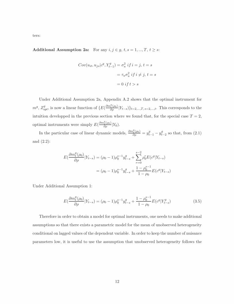
Additional Assumption 2a: For any i, j ( g, t, s = 1, ..., T , t ) s:
Cov(uit, ujs|cg, Y gt"1) = #2
u if i = j, t = s
= 'u#2u if i != j, t = s
= 0 if t > s
Under Additional Assumption 2a, Appendix A.2 shows that the optimal instrument for
mg, Zgopt, is now a linear function of {E(!m
gt ("0)!" |Yt"s)}t=2,...,T, s=2,...,t. This corresponds to the
intuition developped in the previous section where we found that, for the special case T = 2,
optimal instruments were simply E(!mg
2("0)
!" |Y0).
In the particular case of linear dynamic models, !mgt ("0)!" = ygt"1 " ygt"2 so that, from (2.1)
and (2.2):
E("mg
t (!0)
"!|Yt"s) = (!0 " 1)!s"1
0 ygt"s +s"2"
r=0
!r0E(cg|Yt"s)
= (!0 " 1)!s"10 ygt"s +
1" !s"10
1" !0E(cg|Yt"s)
Under Additional Assumption 1:
E("mg
t (!0)
"!|Yt"s) = (!0 " 1)!s"1
0 ygt"s +1" !s"1
0
1" !0E(cg|Y g
t"s) (3.5)
Therefore in order to obtain a model for optimal instruments, one needs to make additional
assumptions so that there exists a parametric model for the mean of unobserved heterogeneity
conditional on lagged values of the dependent variable. In order to keep the number of nuisance
parameters low, it is useful to use the assumption that unobserved heterogeneity follows the
12

simple cluster correlation structure:
Corr(ci, cj) = 'c if i != j, i, j ( g
= 0 otherwise
Also we use the assumption that disturbances {ugt }t=1,...,T are independent from unob-
served heterogeneity, that both have a joint normal distribution and that the initial values of
the dependent variable are in the stationary state associated with (2.1), i.e.:
yg0 =cg
1" !0+ ug0 (3.6)
where ug0 is independent of cg and {ugt }t=1,...,T , follows normal distribution with zero mean,
variance equal to #2u/(1 " !20) and has a within cluster correlation of 'u.5 Let the variance-
covariance matrix of ugt for t = 1, ..., T be denoted by 'gu:
'gu = #2
u
#
$
$
$
$
$
$
$
%
1
'u 1
... ...
'u ... 'u 1
&
'
'
'
'
'
'
'
(
(3.7)
5The auxilliary assumption of stationary initial conditions might be inappropriate for some applications.It would be easy to generalize this assumption, at the cost of introducing two more nuisance parameters, byassuming for instance:
yg0 = !cg + ug
0
ug0|cg & N(0, !0)
V ar(ui0) = $0
Corr(ui0, uj0) = %u if i != j but gi = gj
13

Let the variance-covariance matrix of cg be denoted by 'gc :
'gc = #2
c
#
$
$
$
$
$
$
$
%
1
'c 1
... ...
'c ... 'c 1
&
'
'
'
'
'
'
'
(
(3.8)
The last additional assumption of our model for optimal instruments is:
Additional Assumption 3a: Suppose that for any cluster g = 1, ..., G:
#
$
$
$
$
%
cg
yg0
ug
&
'
'
'
'
(
* N(
#
$
$
$
$
%
µc(ng
11""0
µc(ng
0
&
'
'
'
'
(
,
#
$
$
$
$
%
'gc
11""0
'gc
1(1""0)2
'gc + 1
1""20
'gu
0 0 IT + 'gu
&
'
'
'
'
(
) (3.9)
where 'gc and 'g
u have been defined previously and (ng is a column vector of ones of dimension
ng ' 1.
Note that E(cg |Y gt ) = E(cg|yg0 , cg + ug1, ..., c
g + ugt ). Define V g as:
V g =
#
$
$
$
$
%
'gc
11""0
'gc
1(1""0)2
'gc + 1
1""20
'gu
0 0 IT + 'gu
&
'
'
'
'
(
(3.10)
Under Additional Assumption 3a:
#
$
$
$
$
$
$
$
$
$
$
%
cg
yg0
cg + ug1
...
cg + ugT
&
'
'
'
'
'
'
'
'
'
'
(
* N(µg, AgV gAg") (3.11)
14

where µg = Ag
#
$
$
$
$
%
µc(ng
11""0
µc(ng
0
&
'
'
'
'
(
and Ag is the deterministic matrix of ones and zeros so that
Ag
#
$
$
$
$
%
cg
yg0
ug
&
'
'
'
'
(
=
#
$
$
$
$
$
$
$
$
$
$
%
cg
yg0
cg + ug1
...
cg + ugT
&
'
'
'
'
'
'
'
'
'
'
(
.
Therefore, using the properties of the multivariate normal distribution, E(cg|Yt) can be
obtained as a linear function of yg0 , cg+ug1, ..., c
g+ugt with coe"cients given by the elements of
V g. The exact form of E(cg|Yt) under Additional Assumptions 1, 2a, 3a is given in Appendix
A.3.
Only five nuisance parameters compose V g and can be consistently estimated if a consistent
preliminary estimator of !0 is available, denote it !. Let rit(!) = yit " !yit"1. Consistent
estimators for the nuisance parameters in V can be:
#2u =
1
2
1
T " 1
1
n
T"
t=2
n"
i=1
mit(!)2
'u =1
#2u
1
2
1
T " 1
1
n
T"
t=2
n"
i=1
1
ngi " 1
n"
j=1
1[i != j, gi = gj ]mit(!)mjt(!)
#2c =
1
T (T " 1)
1
n
T"
t=1
T"
s=1
n"
i=1
1[t != s]rit(!)ris(!)" µ2c
µc =1
T
1
n
T"
t=1
n"
i=1
rit(!)
'c =1
#2c
1
T (T " 1)
1
n
T"
t=1
T"
s=1
n"
i=1
1
ngi " 1
n"
j=1
1[t != s, gi = gj ; i != j]rit(!)rjs(!)
Let &g be the consistent estimator for the variance-covariance matrix &g = V ar(mg(!0))
composed of #u and 'u from the formula derived in Appendix A.2. Let &g"1/2 be the upper-
diagonal matrix such that &g"1/2"&g"1/2 = &g"1. Denote &g"1/2t the tth ng'ng(T"1) matrix
15

composing &g"1/2. Let µgct be a consistent estimator of E(cg|Yt) from the formula given in
the Appendix A.3.
A consistent estimator for the optimal instrument for mg(!) under (2.1) and (2.2) and
Assumptions 1, 2a, 3a is:
Zgopt = [&g"1/2
1
#
$
$
$
$
%
(!" 1)yg0 + µgc0
...
!T"2(!" 1)yg0 +1""T#1
1"" µgc0
&
'
'
'
'
(
, ..., &g"1/2T"1
#
$
$
$
$
%
0
...
(!" 1)ygT"2 + µgcT"2
&
'
'
'
'
(
]&g"1/2
(3.12)
and the estimator obtained from using this instrument matrix is defined by:
G"
g=1
Zgoptm
g(!#) = 0 (3.13)
Standard errors for !# that are consistent as long as (2.1), (2.2) and Additional Assumption
1 hold are given by:
s.e. = ((G"
g=1
Zgopt
"mg
"!(!#))"2
G"
g=1
Zgoptm
g(!#)mg(!#)"
Zg"
opt)1/2 (3.14)
The estimator defined by (3.13) is consistent even when the Additional Assumption 1
of cluster sampling is not satisfied. Without Additional Assumption 1 but under regularity
conditions on the strength of the cross-sectional dependence, its asymptotic variance is given
by:
Avar(!) = plim(1
G
G"
g=1
Zgopt
"mg
"!)"2plim((
1
G
G"
g=1
Zgoptm
g)2) (3.15)
Non-parametric estimators for plim(( 1G
!Gg=1 Z
goptm
g)2) and statistical tests with general
forms of spatial dependence are availabe and have been discussed in Conley (1999), Bester
et al. (2011b), Kim and Sun (2011) and Bester et al. (2011a).
In situations where available preliminary estimators might have poor small sample prop-
erties, one can also use an iterated version of the feasible optimal estimator. Denote Zgopt(!)
to be the value of the estimated optimal instruments for a preliminary estimator evaluated at
16

!. The iterated optimal estimator is defined by:
G"
g=1
Zgopt(!iter)m
g(!iter) = 0 (3.16)
This estimator has the same&n-asymptotic properties as the two step estimator defined
by (3.13) but its small sample properties will not depend on the small sample properties of a
preliminary estimator.
3.3 Comparison to Existing Estimators
The estimator defined by (3.13) can be rewritten as !! that satisfies the equation:
G"
g=1
wg!())Zgmg(!!) = 0 (3.17)
where ) = [#2u, 'u, #
2c , µc, 'c], Zg is the matrix containing all valid instruments for mg:
Zg =
#
$
$
$
$
$
$
$
%
Ing + Y g0
0 Ig + Y g1
... ...
0 ... 0 Ing + Y gT"2
&
'
'
'
'
'
'
'
(
(3.18)
and wg!() is the row vector function such that wg!())Zg = Zgopt.
The Arellano and Bond estimator can also be written as exactly identified from:
G"
g=1
wgABZ
gmg(!AB) = 0 (3.19)
where:
wgAB =
n"
i=1
("m
"
"!(!AB)Z
"
i)(n"
i=1
Zimi(!)mi(!AB)"
Z"
i)"1Sg (3.20)
17

where Sg is the matrix of zeros and ones such that SgZgmg(!) =!
i$g Zimi(!) where:
Zi =
#
$
$
$
$
$
$
$
%
Yi0
0 Yi1
... ...
0 ... 0 YiT"2
&
'
'
'
'
'
'
'
(
(3.21)
In the presence of cross-sectional dependence, it is likely that our estimator will perform
better than the Arellano and Bond estimator even when some of the Auxiliary Assumptions
1, 2a, 3a are violated because our estimator gives non-zero weights to moment conditions
obtained from using instruments from neighboring observations. As discussed in previous
sections, these instruments may have significant predictive power for the covariates in the
di!erenced equations so that these additional moment conditions might be useful to improve
the accuracy of the estimator. In addition, our estimator relies on the estimation of only five
nuisance parameters to compute weights for all n2g'T'(T"1)/2 moment conditions available
per cluster whereas the Arellano and Bond estimator relies on the estimation of T ' (T "1)/2
weights. When T is relatively large, estimating that many nuisance parameters causes the
Arellano and Bond estimator to su!er from poor small sample properties in terms of accuracy
and inference, which was studied in the context of cross-sectional independence in Alvarez
and Arellano (2003) and Windmeijer (2005). Section 5 contains additional evidence based on
Monte Carlo simulations that the Arellano and Bond estimator has poor accuracy and biased
inference in small samples both with and without cross-sectional dependence.
So-called system GMM estimators presented in Ahn and Schmidt (1995), Arellano and
Bover (1995), and Blundell and Bond (1998) are similar to the Arellano and Bond estimator
but use additional moment conditions based on additional assumptions of homoscedasticity,
serial correlation or stationary initial conditions. Since our estimator is only based on the
mean independence of transitory shocks conditional on past outcomes, it is more robust than
the estimators presented in Ahn and Schmidt (1995), Arellano and Bover (1995) or Blundell
and Bond (1998).
18

4 Models with Covariates
Similar auxiliary assumptions as in the previous section can be listed to model optimal instru-
ments for models with covariates. In this section we consider a model that allows for some
of the covariates to be strictly exogenous (wit) and some of the covariates to be sequentially
exogenous or contemporaneously endogenous (xit):
yit = xit%0 + wit&0 + ci + uit t = 1, ..., T (4.1)
E(uit|Zt,W ) = 0 (4.2)
where W = [W1, ...,Wn] and Wi = wi1, ..., wiT and Zt = [zi1, ..., zit] and for every random
variable x(j)it in xit, either x(j)it or x(j)it"1 is in zit.6 x(j)it is said to be sequentially exogenous if it
is in zit. If x(j)it"1 only is in zit, x
jit is said to be contemporaneously endogenous. Such a model
specification is flexible enough to allow for complex interactions between unobserved factors
and covariates of interest, an example will be given in Section 6. The estimation method
presented in this section can be generalized to the case where neither xit nor xit"1 are part
of zit but where some other instruments are available. As a notational matter, we generalize
the notation from the previous section by denoting by xg the vector [x1g , ..., xngg ]"
for any
sequence of variables {xi}i=1,...,n.
A consistent estimator of %0, &0 is obtained from the di!erenced equation:
#yit = #xit%0 +#wit&0 +#uit t = 1, ..., T (4.3)
E(#uit|Zt"1,W ) = 0 (4.4)
To model optimal instruments for estimating %0 and &0 from (4.3) and (4.4), we will make
use of the same auxiliary assumption of clustering, i.e. we maintain the use of Additional
Assumption 1a. We also generalize Additional Assumption 2a so that homoscedasticity and
6Note that a special case of this model is the dynamic model we considered in the previous section wherexit = yit#1, xit = zit, and wit&0 = 0. In most applications, even if xit includes other covariates than laggedvalues of the dependent variable, it is expected that yit#1 will be included in xit in order to identify the e"ectof xit on yit separately from the dynamic e"ects in yit and xit.
19

serial correlation are specified conditional on the relevant instruments:
Additional Assumption 2b: For any i, j ( g, t, s = 1, ..., T , t ) s:
Cov(uit, ujs|cg, Zgt ) = #2
u if i = j, t = s
= 'u#2u if i != j, t = s
= 0 if t > s
As in the previous section, this assumption guarantees that the optimal instruments will
be known linear functions of {E(#xit|Zgs ,W g)}t,s=1,...,T, s%t"1 and Wi (up to the unknown
nuisance parameters #2u and 'u). Therefore, we need to generalize Additional Assumption 3a
to obtain a parsimonious model for {E(#xit|Zgs ,W g)}t,s=1,...,T, s%t"1. To do so, we can model
zgt as a VAR process conditional on W g:
Additional Assumption 3b: Suppose that for any observation i = 1, ..., n:
zit = (zit"1 + wit) + di + vit (4.5)
and:#
$
$
$
$
%
dg
zg0
vg
&
'
'
'
'
(
|W g * N(
#
$
$
$
$
%
µd(W g)
µz0(Wg)
0
&
'
'
'
'
(
,
#
$
$
$
$
%
'gd
'dz0 'z0
0 0 'v
&
'
'
'
'
(
(4.6)
where vg = [vg"
1 , ..., vg"
T ]"
.
In particular applications, one will impose auxiliary restrictions on µd(.), µz0(.), 'gd, 'dz0 ,
'z0 , 'v so that they can be estimated with few enough nuisance parameters.
Additional Assumption 3b implies:
E(zit|Zgt"s,W
g) = (szit"s +s"1"
r=0
(r(wit"r) + E(di|Zgt"s,W
g)) (4.7)
20

and:
E(di|Zgt ,W
g) = E(di|zg0 ,Wg, dg + vg1 , ..., d
g + vgt ) (4.8)
which can be derived from Additional Assumption 3b as was done in the previous section. For
any covariate x(j)it , either x(j)it is in zit or x(j)it"1 is in zit, therefore Additional Assumption 3b
yields a model for E(x(j)it |Zgs ,W g) #s , t and hence E(#xit|Zg
s ,W g) #s , t" 1 as a function
of the nuisance parameters in Additional Assumption 3b.
Therefore, under (4.1), (4.2) and Additional Assumptions 1a, 2b and 3b, one can find a
parametric model for the optimal instruments for estimating %0 and &0. A feasible version of
these instruments can be obtained from a preliminary estimator of (%0, )0) as in the previous
section. One can also use an iterated version of this feasible estimator in order to obtain an
estimator with better performances in small samples.
5 Monte Carlo Simulations
In this section we will study the small sample properties of the estimator we propose using
Monte Carlo simulations. Consider the simple data generating process for a model with cluster
correlation and without covariates:
ng * Poisson($) + 1
cg * Fc
yg0 |cg * Normal(µ0(c
g),'0(cg))
ygt |cg, ygt"1, ..., y
g0 * Normal(cg + !ygt"1,'u(c
g, ygt"1, ..., yg0))
We compare the properties of three estimators of !: The estimator defined in Arellano
and Bond (1991) which we call the AB estimator, the estimator defined by (3.16), which
we denote by Estimator 1 and the estimator defined by (3.16) but with estimated within-
cluster correlations replaced by zero which we denote by Estimator 2.7 As a benchmark for
7In most of the scenarios we simulate, transitory shocks will be homoscedastic, serially uncorrelated and thedependent variable will be stationary so that additional moment conditions presented in Arellano and Bover
21

comparison, we also show the results from using an unfeasible optimal estimator (UO) which is
optimal in the class of estimators that use linear functions of the instruments. This estimator
weights optimally all available moment conditions that use linear instruments using the true
unobserved optimal weights so that it is defined by:
G"
g=1
wgZgmg(!UO) = 0
wg = #g"(W g)"1
#g = E(Zg "mg
"!)
W g = E(Zgmgmg"Zg")
When Additional Assumptions 1, 2a, 3a hold, the UO estimator is the same as the es-
timator defined by (3.4) and will be e"cient in the class of estimators using any function
of the instruments. When these assumptions hold, Estimator 1 and the unfeasible optimal
estimator will also be asymptotically equivalent so that, for small samples, the di!erence in
their performances is due to the extra noise in Estimator 1 due to estimating the nuisance pa-
rameters needed. When Additional Assumptions 2a or 3a are violated, the unfeasible optimal
estimator is asymptotically more e"cient than Estimator 1.
Estimator 1 is asymptotically more e"cient than the AB estimator or than Estimator
2 when there exists cross-sectional dependence and Additional Assumptions 1, 2a, 3a hold.
When Additional Assumptions 1, 2a, 3a hold and there is no cross-sectional dependence,
the AB Estimator, Estimator 1 and Estimator 2 have the same asymptotic variance. When
Additional Assumptions 2a or 3a are violated and there is no cross-sectional dependence,
the AB estimator has a smaller asymptotic variance than Estimator 1 but, in finite samples,
Estimator 1 or Estimator 2 might still have better properties than the AB estimator because
they make use of less nuisance parameters. When Additional Assumptions 2a or 3a are
violated and there is cross-sectional dependence, which of the AB estimator or Estimator
1995, Ahn and Schmidt 1995 or Blundell and Bond 1998 hold. We do not present estimators that use thesemoment conditions however since we are interested in studying the properties of estimators that are robust tothese moment conditions being false.
22

1 has smallest asymptotic variance depends on the data generating process but we expect
Estimator 1 to perform better since, by making use of instruments from other observations in
the cluster, it should use a weighted sum of moment conditions that is closer to optimal that
the sum used for the AB estimator.
For inference for the AB estimator, we will consider GMM robust standard errors with
clustered standard errors with and without the finite sample correction proposed by Windmei-
jer (2005). For inference for Estimators 1 and 2, we use the standard errors defined in (3.14)
that only require (2.1), (2.2) and Additional Assumption 1 to hold in order to be consistent.
We will study the small sample properties of the estimators in three di!erent scenarios:
within cluster equi-correlation, cross-sectional independence and general within cluster cor-
relation with unobserved heterogeneity that does not have a Normal distribution. Scenario
1 and 2 will correspond to Additional Assumptions 1, 2a, 3a holding. In Scenario 1 there is
cross-sectional dependence and in Scenario 2 there is no cross-sectional dependence. Scenario
3 corresponds to only Additional Assumption 1 holding.
More precisely, Scenario 1 uses the following parameterization:
Fc = Normal(0,
#
$
$
$
$
$
$
$
%
1
0.5 1
... ...
0.5 ... 0.5 1
&
'
'
'
'
'
'
'
(
)
'u(cg, ygt"1, ..., y
g0) =
#
$
$
$
$
$
$
$
%
1
0.5 1
... ...
0.5 ... 0.5 1
&
'
'
'
'
'
'
'
(
µ0(cg) =
cg
1" !0
'0(cg) =
1
1" !20'u(c
g, ygt"1, ..., yg0)
23

Scenario 2 uses:
Fc = Normal(0,
#
$
$
$
$
$
$
$
%
1
0 1
... ...
0 ... 0 1
&
'
'
'
'
'
'
'
(
)
'u(cg, ygt"1, ..., y
g0) =
#
$
$
$
$
$
$
$
%
1
0 1
... ...
0 ... 0 1
&
'
'
'
'
'
'
'
(
µ0(cg) =
cg
1" !0
'0(cg) =
1
1" !20'u(c
g, ygt"1, ..., yg0)
And Scenario 3 uses:
Fc = LogNormal(0,
#
$
$
$
$
$
$
$
%
1
0.5 1
... ...
0.5 ... 0.5 1
&
'
'
'
'
'
'
'
(
)
'u(cg, ygt"1, ..., y
g0) =
#
$
$
$
$
$
$
$
%
u2i1t"1
0.5ui1t"1ui2t"1 u2i2t"1
... ...
0.5ui1t"1uing t"1 ... 0.5uing#1t"1uing t"1 u2ing t"1
&
'
'
'
'
'
'
'
(
µ0(cg) =
cg
1" !0
'0(cg) =
1
1" !20
#
$
$
$
$
$
$
$
%
1
0.5 1
... ...
0.5 ... 0.5 1
&
'
'
'
'
'
'
'
(
24

All Monte Carlo results were obtained using 1,000 replications. We present results from
simulations conditional on Estimators 1 and 2 converging. Table 1 shows the number of
observations where all estimators converged, which represents all or almost all draws except
when T = 5, G = 100 and ! = 0.8. In this case Estimator 1 or Estimator 2 did not converge in
15%-22% of the replications depending on the scenario. In particular applications, convergence
of Estimators 1 and 2 will depend on the particular numerical algorithm chosen and properties
of the data. For instance in the application presented in Section 6, convergence was achieved
in just a few iterations even though T = 3.
Table 2, 3 and 4 show the results for the four estimators considered in terms of bias,
standard deviation and root mean squared error for a value of ! of 0.8. Table 2 shows results
for the case where there is equicorrelation within clusters, Table 3 the case where there is no
cross-sectional correlation and Table 4 the case where there is heteroscedasticity and cross-
sectional correlation. The first conclusion from these three tables is that Estimator 1 and 2
exhibit virtually no bias compared to the AB estimator. Estimator 1 also has significantly
smaller standard deviations when there is cross-sectional correlation (Scenarios 1 and 3). Both
of these features of our estimator result in significantly smaller values for mean squared error.
The smaller standard deviations of our estimator are due to the use of instruments from other
observations in the cluster that are relevant in the presence of cross-sectional dependence.
The low bias is attributable to our estimators using very few nuisance parameters compared
to the AB estimator. The improvement of Estimator 1 over the AB estimator is particularly
striking when T is large and G is small, which is when the AB estimator uses the most
nuisance parameters compared to the sample size. When there is no within cluster correlation,
Estimators 1 and 2 have standard deviations only slightly lower than the AB estimator so
that the decrease in rmse of Estimators 1 and 2 compared to the AB estimator is mostly
due to the elimination of the bias. In scenario 3 where the unfeasible optimal estimator
is asymptotically more e"cient than Estimator 1, Estimator 1 performs very closely to the
unfeasible optimal estimator, which shows that the approximation of the optimal weighted
sum of moment conditions used by Estimator 1 is good in this case.
25

Table 5, Table 6 and Table 7 show results in terms of bias in standard errors (captured by
the ratio of the mean of the standard errors over the standard deviations of the estimators),
coverage of the 95% confidence interval and average length of 95% confidence intervals. All
three tables show that standard errors for the AB estimator without the Windmeijer correction
are seriously downward biased, particularly when T is large, resulting is very low coverage of
95% confidence intervals. The Windmeijer correction yields unbiased standard errors for the
AB estimator but the resulting confidence intervals still have low coverage because of the bias
in the AB estimator of !0. The standard errors for Estimators 1 and 2 are unbiased and the
resulting confidence intervals have the correct coverage of 95%.
Tables 8-13 show the same results for !0 = 0.5. Estimators 1 and 2 show similar im-
provements over the AB estimator but slightly less markedly since, with this lower level of
persistence, the instruments used by the AB estimator are not as weak as when !0 = 0.8 so
that there is less to gain compared to the unfeasible optimal estimator.
6 Application: Estimation of Persistence in Student Achieve-
ment
In this section we are interested in estimating the e!ect of attending private schools on student
achievement in Punjab, Pakistan. In a non-experimental framework, estimating the causal
e!ects of some factors on student achievement requires accounting for factors that a!ected
student achievements in previous time periods since these factors might a!ect students’ learn-
ing ability in the future but also be correlated across time. Therefore a model for studying
the e!ect of some factor x on student achievement y can be written as in Andrabi et al. (2011)
in its summary of the work in Todd and Wolpin (2003):
yit =t"1"
j=0
$jxit"j +t"1"
j=0
*jµit"j (6.1)
26

where µt are unobserved shocks to student achievement. If one assumes that both {$j}j=1,...,T
and {*j}j=1,...,T form geometric series such that $j = !$j"1 and *j = !*j"1, we can write:
yit"1 = $xit + !yit"1 + µit (6.2)
where *0 was normalized to one.
In order to account for the possibility that students have unobserved characteristics that
a!ect their ability to learn, we can decompose µit between time constant unobserved factors
(also called unobserved heterogeneity) and transitory shocks:
µit = ci + uit (6.3)
where ci is arbitrarily related to xi = [xi1, ..., xiT ] and xit is either strictly exogenous:
E(uit|Xi, Yit"1) = 0 (6.4)
or sequentially exogenous:
E(uit|Xit, Yit"1) = 0 (6.5)
or contemporaneously endogenous:
E(uit|Xit"1, Yit"1) = 0 (6.6)
where Xi = [xi1, ..., xiT ] and Xit"1 = [xi1, ..., xit"1].
In this section we will use the data analyzed in Andrabi et al. (2011) to estimate the
e!ect of attending private schools on student achievement in three districts of Punjab in
Pakistan so that the input of interest is attendance of private school. The other covariates
included are wealth and variables indicating whether each parent lives with the student. We
treat all of these inputs as contemporaneously endogenous since it is likely that they follow a
dynamic process with unobserved transitory shocks that are correlated with shocks to student
27

achievement. For instance, an unobserved and unexpected increase in income might result in a
student enrolling in private school but also benefiting from better study conditions at home so
that Cov(uit, privateschoolit) != 0 while it is still possible that Cov(uit, privateschoolit"1) = 0.
It is likely that transitory shocks are correlated within schools since there are school or
class-level unobserved shocks, such as changes in infrastructure, sta! or teachers, that will
a!ect all students within a school or class. The data-set we use collected between 0 and 25
students per school in each year with most schools being represented by less than 10 students,
which is too small to estimate time-varying school fixed e!ects accurately. Instead, we prefer
treating uit as cross-sectionally correlated. It is likely that unobserved heterogeneity will also
be correlated across students within schools since students might attend specific schools based
on unobserved characteristics, such as residential location, socio-economic characteristics or
past achievements, that relate to their performance. As described in the rest of the paper,
using this cross-sectional correlation for estimation can result in significant e"ciency gains.
For any subject j among English, Urdu and Mathematics (denoted E, U, M), denote by yjit
the grade obtained by student i in year t and subject j and denote by xit the variable indicating
whether student i attended a private school in year t. Let wit be the vector containing other
predetermined explanatory variables for student i at time period t. Denote by ujit transitory
shocks in achievement in subject j and denote measurement error in that achievement by +jit.
Also denote by git the school attended by student i in year t. We will assume clustering so
that, in a given year, transitory shocks are independent across schools. We consider a model
with measurement error and contemporaneously endogenous covariates. As in Andrabi et al.
(2011), we assume that measurement errors are independent across subjects. We can write
such a model as:
yjit = djt + $j0xit + !j0y
jit"1 +wit%
j0 + cji + ujit + +jit " !j0+
jit"1
E(ujit|Xt"1, Yt"1,Wt"1, gt"1) = 0
E(+jit|Xt, Y"jt ,Wt"1, gt"1) = 0
28
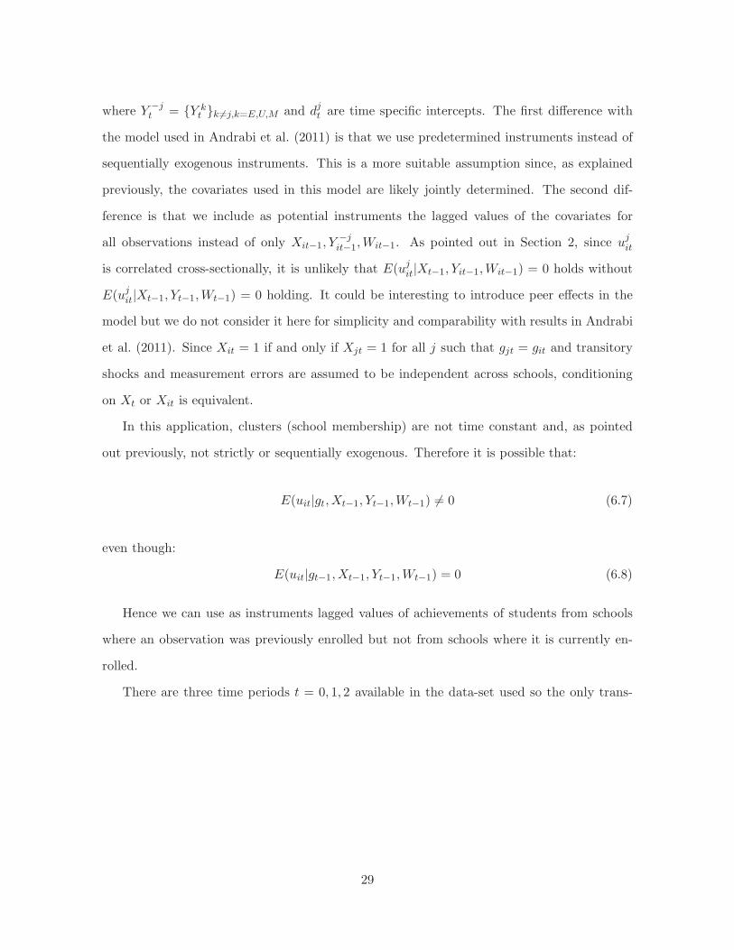
where Y "jt = {Y k
t }k #=j,k=E,U,M and djt are time specific intercepts. The first di!erence with
the model used in Andrabi et al. (2011) is that we use predetermined instruments instead of
sequentially exogenous instruments. This is a more suitable assumption since, as explained
previously, the covariates used in this model are likely jointly determined. The second dif-
ference is that we include as potential instruments the lagged values of the covariates for
all observations instead of only Xit"1, Y"jit"1,Wit"1. As pointed out in Section 2, since ujit
is correlated cross-sectionally, it is unlikely that E(ujit|Xt"1, Yit"1,Wit"1) = 0 holds without
E(ujit|Xt"1, Yt"1,Wt"1) = 0 holding. It could be interesting to introduce peer e!ects in the
model but we do not consider it here for simplicity and comparability with results in Andrabi
et al. (2011). Since Xit = 1 if and only if Xjt = 1 for all j such that gjt = git and transitory
shocks and measurement errors are assumed to be independent across schools, conditioning
on Xt or Xit is equivalent.
In this application, clusters (school membership) are not time constant and, as pointed
out previously, not strictly or sequentially exogenous. Therefore it is possible that:
E(uit|gt,Xt"1, Yt"1,Wt"1) != 0 (6.7)
even though:
E(uit|gt"1,Xt"1, Yt"1,Wt"1) = 0 (6.8)
Hence we can use as instruments lagged values of achievements of students from schools
where an observation was previously enrolled but not from schools where it is currently en-
rolled.
There are three time periods t = 0, 1, 2 available in the data-set used so the only trans-
29

formed equation for each subject that can be used for estimation is:
#yji2 = ,j0 + $j0#xi2 + !j0#yji1 +#wi2%
j0 +#uji2 +#+ji2 " !#+ji1 (6.9)
E(#uji2|X0, Y"j0 ,W0, g0) = 0 (6.10)
E(#+ji2|X0, Y"j0 ,W0, g0) = 0 (6.11)
E(#+ji2|X0, Y"j0 ,W0, g0) = 0 (6.12)
where ,j0 = dj2 " dj1.
Let -j = [,j ,$j , !j,%j" ]"
, mji (-
j) = #yji2 " (,j + $j#xi2 + !j#yji1 + #wi2%j) and mji =
mji (-
j0). The Arellano and Bond estimator for this model is defined by:
-jAB = argmin$j (
n"
i=1
ZjABi mj
i (-j))
"
(n"
i=1
ZjABi mj
i (-j)mj
i (-j)
"
ZjAB"
i )"1(n"
i=1
ZjABi mj
i (-j))
(6.13)
where -j is a preliminary estimator of -j0 and ZjAB
i = [1, y"ji0 , xi0, wi0]
"
.
This estimator is ine"cient because it ignores cross-sectional dependence8. Using the
previous results in this paper, we can specify auxiliary assumptions so that an estimator can
be derived which will be consistent as long as the identifying assumptions defined above hold
and e"cient if the auxiliary assumptions also hold.
The first auxiliary assumption we can use is of conditional homoscedasticity and cluster
equicorrelation. For j = U,E,M :
Cov(ujit, ujls|Y
"j0 ,X0,W0, g0) = #2
uj if i = l, t = s
= 'j#2uj if i != j, git = gls, t = s
= 0 otherwise
8Without measurement error, it would also be possible to use correlation of transitory shocks across out-comes to obtain an e#cient joint estimator of {'j}j=U,E,M . However because of measurement error, the sets ofinstruments across subjects are non-overlapping, so that optimal instruments cannot be derived. Since thereis no restriction in the parameters across equations, weighting of optimally weighted moment conditions orminimum distance methods cannot be used either.
30

and:
Cov(ujit, +jls|Y
"j0 ,X0,W0, g0) = 0# i, l, j, k, t, s
Cov(+jit, +jls|Y
"j0 ,X0,W0, g0) = #2
%j if i = l, j = k, t = s
= 0 otherwise
Under this assumption:
Cov(mji ,m
jl |Y
"j0 ,X0,W, g0) = 2#2
uj + 2#2%j(1 + !+ !2) if i = j
= 'j#2uj(1[gi1 = gl1] + 1[gi2 = gl2]) if i != j
Under the previous auxiliary assumption, the optimal instruments for mji (-
j) will be linear
functions of E(#yji1|Y"j0 ,X0,W0, g0), E(#xi2|Y "j
0 ,X0,W0, g0) and E(#wi2|Y "j0 ,X0,W0, g0).
Since we have T = 2 so that there is only one transformed equation available for estimation,
we can use the simple second auxiliary assumption:
E(#yji1|Y"j0 ,X0,W0, g0) = aj0 +
"
k #=j
aj01kyki0 +
"
k #=j
aj02k1
#gi0
"
l$gi0
ykl0 + aj03xi0
+ aj04wi0 + aj051
#gi0
"
l$gi0
wl0 (6.14)
E(#zi2|Y "j0 ,X0,W0, g0) = bjz0 +
"
k #=j
bjz01kyki0 +
"
k #=j
bjz02k1
#gi0
"
l$gi0
ykl0 + bjz03xi0
+ bjz04wi0 + bjz051
#gi0
"
l$gi0
wl0 (6.15)
where z ( {x,w}and consistently estimate these unknown parameters by OLS regression.
Define E!yj
i , E!xj
i and E!wj
i to be the estimated conditional expectations defined by
(6.14) and (6.15). Define:
Dj"
i =
#
$
$
$
$
%
E!yj
i
E!xj
i
E!wj
i
&
'
'
'
'
(
(6.16)
31

andDj" = [Dj"
1 , ...,Dj"n ]. Define 'j(-j) = [ ˆCov(mj
i (-j),mj
l (-j))]l=1,...,n
i=1,...,n andmj(-j) = [mj"
1 (-j), ...,mj"
n (-j)]"
.
The e"cient estimator for -j0 under the auxiliary assumptions is -j
opt defined by:
Dj"'(-jopt)
"1m(-jopt) = 0 (6.17)
Let M j"
i =
#
$
$
$
$
%
#yj1
#xi2
#wi2
&
'
'
'
'
(
= (!mj
i ($)
!$" )"
. Both the Arellano and Bond estimator and our optimal
estimator can be written as:n"
i=1
Zji m
ji (-
j) = 0 (6.18)
where for the Arellano and Bond estimator, Zji = (
!nl=1M
j"
l ZjAB"
l ))jAB"1ZjABi with )jAB =
!ni=1 Z
jABi mj
i (-j)mj
i (-j)
"
ZjAB"
i . For our optimal estimator, Zji is the i
th column ofDj"'j(-jopt)
"1.
Under the assumption that transitory shocks are independent across schools, -j is consis-
tent for -j0 and asymptotically normal. The asymptotic variance-covariance matrix of both
estimators is9:
AV ar(-) = A"
BA
A = plim(1
n
n"
i=1
ZjiM
ji )
"1
B = plim(1
n
n"
i=1
Zjim
ji
n"
l=1
1[{git = gls}t,s=1,2]mj"
l Zj"
l )
which can be estimated consistently since there is a small number of observations in each
school.
The students’ achievement in each subject was measured by the results obtained by stu-
dents on a test administed by the authors of Andrabi et al. (2011) and graded using the Iterm
Response Theory so that scores can be compared across years and the standard deviation of
scores in the first year (third grade) is one. Table 14 shows the average and standard deviations
9Note that clustering standard errors by the first school attended, which is used in Andrabi et al. (2011),is not justified since transitory shocks should be correlated within a school that a child is currently attendingand not necessarily only across students who attended the same school in the first time period.
32

of scores by subject and grade. Table 15 reports the estimated degree of persistence and the
estimated e!ect of attending private schools on performance for the three subjects considered.
We also show the associated standard errors and 95% confidence intervals. Similarly as in
Andrabi et al. (2011), we find that there is significant persistence in scores except for Mathe-
matics. We estimate e!ects of attending private school that are smaller than in Andrabi et al.
(2011), which can be attributed to Andrabi et al. (2011) treating the covariates as sequentially
exogenous instead of contemporaneously endogenous while it is likely that unobserved factors
simultaneously a!ect performance and school attendance, as explained previously. The op-
timal estimator we presented in this section yields smaller standard errors compared to the
Arellano and Bond estimator both for estimating persistence in student achievements and
for estimating the e!ect of attending private school, with particularly significantly smaller
standard errors for the latter.
7 Conclusion
We have presented an estimation method that used cross-sectional dependence to improve
the accuracy with which dynamic models of panel data are estimated while making use of
few nuisance parameters and being robust to the misspecification of the form of the cross-
sectional dependence. This method can be generalized to models with covariates that are
strictly exogenous, sequentially exogenous or contemporaneoulsy endogenous.
Monte Carlo simulations and an application to the estimation of a value-added model show
that, when there is cross-sectional dependence, this method dominates existing estimators in
terms of accuracy and quality of inference.
Extensions of this work that are the subject of ongoing research consider the generaliza-
tion of the results in this paper to non-linear panel data models, the use of other forms of
cross-sectional dependence than clustering in the auxilliary restrictions, and the asymptotic
properties of our estimator with large numbers of time period and of observations within
clusters.
33

Appendix
A E!cient Estimation with Clustering
A.1 Unfeasible Optimal Instruments
Consider any GMM estimator of !0 defined as in (2.6) for some set of valid instruments
{Zi}i=1,...,n of dimension r ' (T " 1) which can be rewritten as:
! = argmin"(G"
g=1
Zgmg(!))"
$G"
g=1
Zgmg(!) (A.1)
where Zg = [Zg2 , ..., Z
gT ] and Zg
t = [Zi1t, ..., Zing t].
From White (2001), ! is consistent for !0 and:
&G(!" !0)
d$ N(0, (D"
$D)"1D"
$%$D(D"
$D)"1) (A.2)
with D = plim( 1G
!Gg=1 Z
g !mg
!" ) and % = plim( 1G
!Gg=1 Z
gmgmg"Zg").
$ = %"1 is the optimal weighting matrix for that estimator and with such weighting
matrix:&G(!" !0)
d$ N(0, (D"
%"1D)"1) (A.3)
Therefore in this section we will show that the asymptotic variance of !opt defined by (3.4)
is smaller than (D"
%"1D)"1 for any set of valid matrices of instruments {Zi}i=1,...,n as long
as (2.1), (2.2) and Additional Assumption 1 are satisfied.
Since &g"1/2 is upper triangular with its element in row j, column i being a function of
Y gmax{i,j}"1, for any valid set of instruments {Zg}g=1,...,G we have:
E(Zg(&g)"1/2mg) = 0 (A.4)
because the jth r ' ng component of Zg(&g)"1/2 is a function of Y gj"1.
34

In addition, we have:
V ar(Zg(&g)"1/2mg) = E(Zg(&g)"1/2&g(&g)"1/2"Zg")
= E(ZgZg")
because the jth r'ng component of Zg(&g)"1/2 is a function of Y gj"1 and &g = [E(mg
tmg"s |Y g
max{t,s}"2)]s=2,...,Tt=2,...,T
Note that since E((Zgmgmg"Zg")" V ar(Zgmg)) = 0, then plim 1G
!Gg=1(Z
gmgmg"Zg") =
plim 1G
!Gg=1 V ar(Zgmg).
Define:
"mg
"!= (&g)"1/2 "m
g
"!(A.5)
Define !mgt
!" the tth block of ng rows of !mg
!" . Define:
L#gt = E(
"mgt
"!|Yt"2) (A.6)
Define L#g = [L#g"
2 , ..., L#g"
T ] and:
Zgopt = L#g(&g)"1/2 (A.7)
Define Dopt = plim( 1G
!Gg=1 Z
gopt
!mg
! ) and %opt = plim( 1G
!Gg=1 Z
goptm
gmg"Zg"
opt).
E(Zgopt
!mg
! " L#gL#g") = 0 because the jth r ' ng component of Zg&g"1/2 is a function of
Y gj"1 and L#g
t = E(!mgt
!" |Yt"2) therefore:
Dopt = plim(1
G
G"
g=1
Zgopt
"mg
")
= plim(1
G
G"
g=1
L#gL#g")
Since V ar(Zg(&g)"1/2mg) = E(ZgZg") we have in particular: V ar(L#g(&g)"1/2mg) =
35

E(L#gL#g"). Therefore:
%opt = plim(1
G
G"
g=1
Zgoptm
gmg"Zg"
opt)
= plim(1
G
G"
g=1
L#gL#g")
= Dopt
so that (D"
opt%"1optDopt)"1 = D"1
opt.
Therefore the estimator !opt defined by:
!opt = argmin"(G"
g=1
Zgoptm
g(!))"
G"
g=1
Zgoptm
g(!) (A.8)
is consistent for !0 and&G-asymtotically normal with asymptotic variance:
Vopt = D"1opt (A.9)
We can show that this variance-covariance matrix is smaller than (D"
%"1D)"1 no matter
what set of instruments {Zg}g=1,...,G is used. Denote # the di!erence between D"
%"1D and
Dopt:
D = D"
%"1D "Dopt
= D"
%"1D " plim(1
G
G"
g=1
L#gL#g")
= D"
%"1D " plim(1
G
G"
g=1
Zgopt&
gZg"
opt)
Since (&g)"1/2"(&g)"1/2 = (&g)"1 we also have &g = &g1/2&g1/2" where &g1/2 is upper
triangular and is composed of ng ' ng matrices such that the (j, k)th matrix for k > j is a
36

function of Y gk"1. Therefore:
E(Zg("mg(!0)
"!" &gZg"
opt)) = 0 (A.10)
since the jth r'ng component of Zg is a function of Y gj"1 and (&g)1/2t L#g
t = E((&g)1/2 !mgt
!" |Yt"2)
where (&g)1/2t is the (t" 1)th ng ' ng(T " 1) matrix composing (&g)1/2.
In addition we have
E(Zg(mg(!0)mg(!0)
"
" &g)Zg") = 0 (A.11)
We can then apply the WLLN to show that:
D = plim(1
G
G"
g=1
Zg&gZg"
opt)
% = plim(1
G
G"
g=1
Zg&gZg")
Define Dn = 1G
!Gg=1 Z
g&gZg"
opt, %n = 1G
!Gg=1 Z
g&gZg" and D#n = 1
G
!Gg=1 Z
gopt&
gZg"
opt.
Define Z# = [Z1"opt, ..., Z
G"
opt]"
, Z = [Z"
1, ..., Z"
G]"
, S = diag({&g}g=1,...,G), then:
D"
n%"1n Dn "G#
n = Z#"SZ(Z"
SZ)"1Z"
SZ# " Z#"SZ#
= Z#"S1/2(S1/2Z(Z"
SZ)"1Z"
S1/2 " IT&n)S1/2Z
ThereforeD"
n%"1n Dn"D#
n is positive semi-definite for any value of n. ThereforeD"
%"1D"
Dopt is positive semi-definite by the continuous mapping theorem. A similar result was found
in Chamberlain (1992) for the case of cross-sectional independence.
37

A.2 E!cient Estimation with Additional Auxiliary Assumptions
Under Additional Assumptions 1-2a, the variance-covariance matrix of ugt is:
'gu = #2
u
#
$
$
$
$
$
$
$
%
1
'u 1
... ...
'u ... 'u 1
&
'
'
'
'
'
'
'
(
(A.12)
and we have
E(mgtm
g"s |Ymax{t,s}"2) = 2'g
u if t = s
= "'gu if |t" s| = 1
= 0 if |t" s| ) 2
Therefore:
&g = Jg(IT +'g)Jg" (A.13)
where:
Jg =
#
$
$
$
$
$
$
$
%
"1 0 ... 0 1 0 ... 0
0 "1 0 ... 0 1 ... 0
...
0 ... 0 "1 ... 0 1
&
'
'
'
'
'
'
'
(
(A.14)
is the deterministic di!erencing matrix such that Jgug = mg.
Therefore L#gt = &g"1/2E(!m
g
!" |Yt"2) and
Zgopt = [E(
"mg
"!|Y0)
"
, ..., E("mg
"!|YT"2)
"
]*g&g"1/2 (A.15)
38

where:
*g =
#
$
$
$
$
$
$
$
%
&g"1/2"
1 0 ... 0
0 &g"1/2"
2 ...
... ... 0
0 ... 0 &g"1/2"
T"1
&
'
'
'
'
'
'
'
(
(A.16)
where &g"1/2j is the jth ng ' ng(T " 1) matrix composing (&g)"1/2.
A.3 Conditional Expectation of Unobserved Heterogeneity under Cluster-
ing
Under Additional Assumption 1, 2a, 3a we have:
#
$
$
$
$
$
$
$
$
$
$
%
cg
yg0
cg + ug1
...
cg + ugT
&
'
'
'
'
'
'
'
'
'
'
(
* N(µg, AgV gAg") (A.17)
Therefore, using the properties of the multivariate normal distribution, we have:
E(cg|
#
$
$
$
$
$
$
$
%
yg0
cg + ug1
...
cg + ugT
&
'
'
'
'
'
'
'
(
) = µc(ng +AgV gAg"
12AgV gAg""1
22 (
#
$
$
$
$
$
$
$
%
yg0
cg + ug1
...
cg + ugT
&
'
'
'
'
'
'
'
(
"
#
$
%
µc(T&ng
11""0
µc(ng
&
'
(
) (A.18)
where AgV gAg"
12 = Cov(cg,
#
$
$
$
$
$
$
$
%
yg0
cg + ug1
...
cg + ugT
&
'
'
'
'
'
'
'
(
) and AgV gAg"
22 = V ar(
#
$
$
$
$
$
$
$
%
yg0
cg + ug1
...
cg + ugT
&
'
'
'
'
'
'
'
(
) and both matrices
are components of AgV gAg" .
39

E(cg|
#
$
$
$
$
$
$
$
%
yg0
cg + ug1
...
cg + ugt
&
'
'
'
'
'
'
'
(
) can be obtained in a similar fashion by considering only the first ((t +
2)ng)' ((t+ 2)ng) block of AgV gAg"
40

References
Ahn SC, Schmidt P. 1995. E"cient estimation of models for dynamic panel data. Journal of
Econometrics 68: 5–27. ISSN 0304-4076.
URL http://www.sciencedirect.com/science/article/pii/030440769401641C
Alvarez J, Arellano M. 2003. The time series and cross-section asymptotics of dynamic panel
data estimators. Econometrica 71. ISSN 1468-0262.
URL http://www.jstor.org/stable/1555492
Alvarez J, Arellano M. 2004. Robust likelihood estimation of dynamic panel data models.
CEMFI Working Paper 0421 .
URL http://www.cemfi.es/ftp/wp/0421.pdf
Anderson TW, Hsiao C. 1981. Estimation of dynamic models with error components. Journal
of the American Statistical Association 76: 598–606. ISSN 0162-1459.
URL http://www.tandfonline.com/doi/abs/10.1080/01621459.1981.10477691
Andrabi T, Das J, Ijaz Khwaja A, Zajonc T. 2011. Do value-added estimates add value?
accounting for learning dynamics. American Economic Journal. Applied Economics 3: 29–
54. ISSN 19457782.
URL http://www.aeaweb.org/articles.php?doi=10.1257/app.3.3.29
Arellano M. 2003. Modelling optimal instrumental variables for dynamic panel data models.
CEMFI Working Paper .
URL ftp://ftp.cemfi.es/pdf/papers/ma/siv2003.pdf
Arellano M, Bond S. 1991. Some tests of specification for panel data: Monte carlo evidence
and an application to employment equations. The Review of Economic Studies 58: 277–
297. ISSN 0034-6527.
URL http://www.jstor.org/stable/2297968
Arellano M, Bover O. 1995. Another look at the instrumental variable estimation of error-
41

components models. Journal of Econometrics 68: 29–51. ISSN 0304-4076.
URL http://www.sciencedirect.com/science/article/pii/030440769401642D
Balasubramanian N, Sivadasan J. 2010. What happens when firms patent? new evidence
from U.S. economic census data. Review of Economics and Statistics 93: 126–146. ISSN
0034-6535.
URL http://ideas.repec.org/a/tpr/restat/v93y2011i1p126-146.html
Baltagi BH, Fingleton B, Pirotte A. 2013. Estimating and forecasting with a dynamic spatial
panel data model. Oxford Bulletin of Economics and Statistics ISSN 1468-0084.
URL http://onlinelibrary.wiley.com/doi/10.1111/obes.12011/abstract
Bester CA, Conley TG, Hansen CB. 2011a. Inference with dependent data using cluster
covariance estimators. Journal of Econometrics 165: 137–151. ISSN 0304-4076.
URL http://www.sciencedirect.com/science/article/pii/S0304407611000431
Bester CA, Conley TG, Hansen CB, Vogelsang TJ. 2011b. Fixed-b asymptotics for spatially
dependent robust nonparametric covariance matrix estimators. Working Paper .
URL https://www.msu.edu/ tjv/spatialhac.pdf
Blundell R, Bond S. 1998. Initial conditions and moment restrictions in dynamic panel data
models. Journal of Econometrics 87: 115–143. ISSN 0304-4076.
URL http://www.sciencedirect.com/science/article/pii/S0304407698000098
Chamberlain G. 1992. Comment: Sequential moment restrictions in panel data. Journal of
Business & Economic Statistics 10: 20–26. ISSN 0735-0015.
URL http://www.jstor.org/stable/1391799
Cizek P, Jacobs JPAM, Ligthart JE, Vrijburg H. 2011. GMM estimation of fixed e!ects
dynamic panel data models with spatial lag and spatial errors. Discussion Paper 2011-134,
Tilburg University, Center for Economic Research.
URL http://ideas.repec.org/p/dgr/kubcen/2011134.html
42

Conley T. 1999. GMM estimation with cross sectional dependence. Journal of Econometrics
92: 1–45. ISSN 0304-4076.
URL http://www.sciencedirect.com/science/article/pii/S0304407698000840
de Brauw A, Giles J. 2008. Migrant labor markets and the welfare of rural households in the
developing world: Evidence from china. 2008 Annual Meeting, July 27-29, 2008, Orlando,
Florida 6085, American Agricultural Economics Association.
URL http://ideas.repec.org/p/ags/aaea08/6085.html
Donald SG, Imbens GW, Newey WK. 2009. Choosing instrumental variables in conditional
moment restriction models. Journal of Econometrics 152: 28–36. ISSN 0304-4076.
URL http://www.sciencedirect.com/science/article/pii/S0304407609000566
Elhorst JP. 2005. Unconditional maximum likelihood estimation of linear and log-linear
dynamic models for spatial panels. Geographical Analysis 37. ISSN 1538-4632.
URL http://onlinelibrary.wiley.com/doi/10.1111/j.1538-4632.2005.00577.x/abstract
Hahn J. 1997. E"cient estimation of panel data models with sequential moment restrictions.
Journal of Econometrics 79: 1–21. ISSN 0304-4076.
URL http://www.sciencedirect.com/science/article/pii/S0304407697000122
Hsiao C, Pesaran HM, Tahmiscioglu KA. 2002. Maximum likelihood estimation of fixed
e!ects dynamic panel data models covering short time periods. Journal of Econometrics
109: 107–150. ISSN 0304-4076.
URL http://www.sciencedirect.com/science/article/pii/S0304407601001439
Jenish N, Prucha IR. 2009. Central limit theorems and uniform laws of large numbers for
arrays of random fields. Journal of Econometrics 150: 86–98. ISSN 0304-4076.
URL http://www.sciencedirect.com/science/article/pii/S0304407609000475
Jenish N, Prucha IR. 2012. On spatial processes and asymptotic inference under near-epoch
dependence. Journal of Econometrics 170: 178–190. ISSN 0304-4076.
URL http://www.sciencedirect.com/science/article/pii/S0304407612001340
43

Kim MS, Sun Y. 2011. Spatial heteroskedasticity and autocorrelation consistent estimation
of covariance matrix. Journal of Econometrics 160: 349–371. ISSN 0304-4076.
URL http://www.sciencedirect.com/science/article/pii/S0304407610002034
Kuersteiner GM, Prucha IR. 2013. Limit theory for panel data models with cross sectional
dependence and sequential exogeneity. Journal of Econometrics 174: 107–126. ISSN 0304-
4076.
URL http://www.sciencedirect.com/science/article/pii/S0304407613000389
Mutl J. 2006. Dynamic panel data models with spatially correlated disturbances. University
of Maryland Theses and Dissertations .
URL http://hdl.handle.net/1903/3729
Su L, Yang Z. 2013. QML estimation of dynamic panel data models with spatial errors.
Research Collection School of Economics (Open Access) .
URL http://ink.library.smu.edu.sg/soe research/1490
Todd PE, Wolpin KI. 2003. On the specification and estimation of the production function
for cognitive achievement*. The Economic Journal 113. ISSN 1468-0297.
URL http://onlinelibrary.wiley.com/doi/10.1111/1468-0297.00097/abstract
Topalova P, Khandelwal A. 2010. Trade liberalization and firm productivity: The case of
india. Review of Economics and Statistics 93: 995–1009. ISSN 0034-6535.
URL http://ideas.repec.org/p/imf/imfwpa/04-28.html
White H. 2001. Asymptotic theory for econometricians. San Diego: Academic Press. ISBN
0127466525 9780127466521.
Windmeijer F. 2005. A finite sample correction for the variance of linear e"cient two-step
GMM estimators. Journal of Econometrics 126: 25–51. ISSN 0304-4076.
URL http://www.sciencedirect.com/science/article/pii/S0304407604000387
44
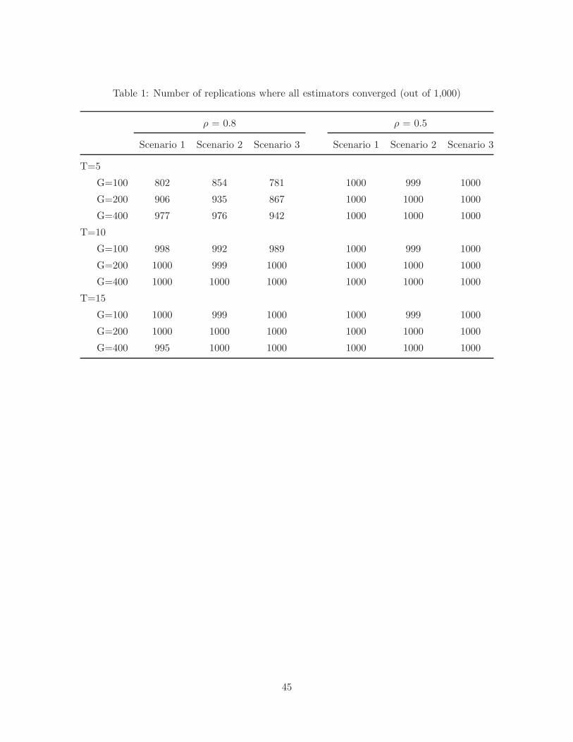
Table 1: Number of replications where all estimators converged (out of 1,000)
! = 0.8 ! = 0.5
Scenario 1 Scenario 2 Scenario 3 Scenario 1 Scenario 2 Scenario 3
T=5
G=100 802 854 781 1000 999 1000
G=200 906 935 867 1000 1000 1000
G=400 977 976 942 1000 1000 1000
T=10
G=100 998 992 989 1000 999 1000
G=200 1000 999 1000 1000 1000 1000
G=400 1000 1000 1000 1000 1000 1000
T=15
G=100 1000 999 1000 1000 999 1000
G=200 1000 1000 1000 1000 1000 1000
G=400 995 1000 1000 1000 1000 1000
45

Table 2: Bias and RMSE, ! = .8, equicorrelation within clusters
UnfeasibleOptimalEstimator
Arellanoand BondEstimator
Estimator 1 Estimator 2
T=5
G=100 bias "0.031 "0.158 "0.037 "0.045
sd 0.121 0.176 0.137 0.191
rmse 0.125 0.236 0.142 0.196
G=200 bias "0.018 "0.087 "0.018 "0.025
sd 0.089 0.127 0.093 0.134
rmse 0.091 0.154 0.095 0.136
G=400 bias "0.001 "0.033 "0.002 0.000
sd 0.064 0.092 0.065 0.097
rmse 0.064 0.098 0.065 0.097
T=10
G=100 bias 0.001 "0.060 0.001 0.001
sd 0.047 0.067 0.048 0.068
rmse 0.047 0.090 0.048 0.068
G=200 bias "0.001 "0.033 "0.001 "0.003
sd 0.034 0.048 0.034 0.047
rmse 0.034 0.058 0.034 0.047
G=400 bias 0.001 "0.016 0.001 0.000
sd 0.024 0.035 0.024 0.034
rmse 0.024 0.038 0.024 0.034
T=15
G=100 bias "0.001 "0.041 "0.000 "0.003
sd 0.028 0.038 0.028 0.037
rmse 0.028 0.056 0.028 0.037
G=200 bias 0.000 "0.022 0.000 "0.001
sd 0.018 0.027 0.018 0.026
rmse 0.018 0.034 0.018 0.026
G=400 bias 0.000 "0.010 0.000 0.000
sd 0.013 0.019 0.013 0.018
rmse 0.013 0.021 0.013 0.018
46

Table 3: Bias and RMSE, ! = .8, no correlation within clusters
UnfeasibleOptimalEstimator
Arellanoand BondEstimator
Estimator 1 Estimator 2
T=5
G=100 bias "0.028 "0.097 "0.030 "0.034
sd 0.121 0.119 0.135 0.127
rmse 0.124 0.153 0.138 0.131
G=200 bias "0.013 "0.046 "0.013 "0.014
sd 0.093 0.091 0.097 0.094
rmse 0.093 0.102 0.098 0.095
G=400 bias "0.001 "0.020 "0.001 "0.002
sd 0.063 0.063 0.066 0.065
rmse 0.063 0.066 0.066 0.065
T=10
G=100 bias 0.000 "0.033 0.000 "0.000
sd 0.046 0.050 0.047 0.047
rmse 0.046 0.060 0.047 0.047
G=200 bias "0.001 "0.018 "0.001 "0.002
sd 0.033 0.035 0.033 0.033
rmse 0.033 0.039 0.033 0.033
G=400 bias 0.001 "0.008 0.001 0.001
sd 0.024 0.025 0.024 0.024
rmse 0.024 0.026 0.024 0.024
T=15
G=100 bias "0.001 "0.023 "0.001 "0.001
sd 0.028 0.031 0.028 0.028
rmse 0.028 0.038 0.028 0.028
G=200 bias 0.000 "0.011 0.000 0.000
sd 0.018 0.020 0.018 0.018
rmse 0.018 0.023 0.018 0.018
G=400 bias 0.000 "0.005 0.000 0.000
sd 0.013 0.013 0.013 0.013
rmse 0.013 0.014 0.013 0.013
47

Table 4: Bias and RMSE, ! = .8, heteroscedasticity and correlation within clusters
UnfeasibleOptimalEstimator
Arellanoand BondEstimator
Estimator 1 Estimator 2
T=5
G=100 bias "0.027 "0.226 "0.065 "0.049
sd 0.183 0.218 0.271 0.367
rmse 0.185 0.314 0.279 0.370
G=200 bias "0.025 "0.140 "0.027 "0.033
sd 0.125 0.166 0.135 0.203
rmse 0.128 0.217 0.137 0.206
G=400 bias "0.007 "0.069 "0.008 "0.010
sd 0.084 0.121 0.085 0.131
rmse 0.085 0.139 0.086 0.131
T=10
G=100 bias 0.001 "0.075 "0.000 0.000
sd 0.055 0.075 0.056 0.074
rmse 0.055 0.106 0.056 0.074
G=200 bias 0.000 "0.042 0.000 "0.000
sd 0.039 0.055 0.039 0.054
rmse 0.039 0.069 0.039 0.054
G=400 bias 0.001 "0.019 0.001 0.001
sd 0.027 0.039 0.027 0.038
rmse 0.027 0.043 0.027 0.038
T=15
G=100 bias "0.001 "0.046 "0.000 "0.002
sd 0.031 0.041 0.030 0.040
rmse 0.031 0.062 0.030 0.040
G=200 bias 0.001 "0.024 0.001 0.000
sd 0.020 0.029 0.020 0.028
rmse 0.020 0.037 0.020 0.028
G=400 bias 0.001 "0.012 0.000 0.000
sd 0.015 0.021 0.014 0.020
rmse 0.015 0.024 0.014 0.020
48

Table 5: Inference, ! = .8, equicorrelation within clusters
UnfeasibleOptimalEstimator
Arellanoand BondEstimator
AB w/Windmeijercorrection
Estimator 1 Estimator 2
T=5
G=100 ratio 1.121 0.788 1.051 1.016 1.002
coverage 0.969 0.763 0.895 0.964 0.959
length 0.539 0.550 0.749 0.552 0.760
G=200 ratio 1.063 0.834 1.045 1.024 0.978
coverage 0.956 0.796 0.917 0.951 0.956
length 0.375 0.417 0.525 0.376 0.518
G=400 ratio 1.073 0.863 1.029 1.042 0.977
coverage 0.976 0.888 0.939 0.969 0.954
length 0.268 0.313 0.376 0.268 0.372
T=10
G=100 ratio 0.987 0.661 1.004 0.962 0.943
coverage 0.948 0.653 0.873 0.952 0.949
length 0.184 0.176 0.270 0.184 0.254
G=200 ratio 0.983 0.734 1.003 0.975 0.961
coverage 0.949 0.760 0.905 0.949 0.944
length 0.130 0.139 0.194 0.130 0.179
G=400 ratio 0.974 0.766 0.975 0.968 0.943
coverage 0.953 0.835 0.922 0.952 0.939
length 0.092 0.104 0.134 0.091 0.127
T=15
G=100 ratio 0.941 0.561 1.015 0.939 0.983
coverage 0.941 0.480 0.815 0.943 0.948
length 0.105 0.084 0.140 0.105 0.144
G=200 ratio 1.025 0.688 1.053 1.022 1.006
coverage 0.961 0.696 0.916 0.958 0.951
length 0.074 0.072 0.110 0.074 0.102
G=400 ratio 1.012 0.763 1.024 1.013 1.006
coverage 0.952 0.823 0.925 0.957 0.944
length 0.052 0.057 0.078 0.052 0.072
49

Table 6: Inference, ! = .8, no correlation within clusters
UnfeasibleOptimalEstimator
Arellanoand BondEstimator
AB w/Windmeijercorrection
Estimator 1 Estimator 2
T=5
G=100 ratio 1.140 1.042 1.142 1.013 1.060
coverage 0.978 0.883 0.923 0.959 0.960
length 0.548 0.491 0.558 0.542 0.533
G=200 ratio 1.038 1.000 1.053 0.984 1.004
coverage 0.961 0.909 0.932 0.954 0.948
length 0.379 0.359 0.383 0.377 0.372
G=400 ratio 1.082 1.052 1.073 1.040 1.041
coverage 0.975 0.947 0.951 0.968 0.965
length 0.269 0.262 0.271 0.268 0.267
T=10
G=100 ratio 1.006 0.820 1.007 0.974 0.975
coverage 0.958 0.836 0.910 0.951 0.952
length 0.185 0.163 0.204 0.182 0.182
G=200 ratio 0.990 0.890 0.971 0.981 0.979
coverage 0.950 0.884 0.918 0.951 0.949
length 0.130 0.122 0.142 0.129 0.129
G=400 ratio 0.976 0.920 0.975 0.964 0.965
coverage 0.952 0.914 0.932 0.950 0.950
length 0.092 0.089 0.097 0.091 0.091
T=15
G=100 ratio 0.949 0.686 0.959 0.935 0.937
coverage 0.948 0.730 0.866 0.943 0.944
length 0.106 0.084 0.105 0.105 0.105
G=200 ratio 1.027 0.846 1.021 1.022 1.020
coverage 0.962 0.860 0.925 0.957 0.958
length 0.074 0.066 0.082 0.074 0.074
G=400 ratio 1.011 0.935 1.033 1.008 1.009
coverage 0.952 0.902 0.945 0.955 0.956
length 0.052 0.050 0.058 0.052 0.052
50

Table 7: Inference, ! = .8, heteroscedasticity and correlation within clusters
UnfeasibleOptimalEstimator
Arellanoand BondEstimator
AB w/Windmeijercorrection
Estimator 1 Estimator 2
T=5
G=100 ratio 1.027 0.773 1.088 0.834 0.812
coverage 0.963 0.666 0.872 0.949 0.940
length 0.747 0.669 0.943 0.897 1.181
G=200 ratio 1.028 0.801 1.033 0.943 0.854
coverage 0.945 0.736 0.884 0.955 0.934
length 0.507 0.523 0.680 0.501 0.684
G=400 ratio 1.078 0.845 1.027 1.036 0.919
coverage 0.969 0.831 0.901 0.960 0.947
length 0.358 0.402 0.491 0.348 0.474
T=10
G=100 ratio 0.973 0.652 1.009 0.937 0.954
coverage 0.948 0.608 0.857 0.942 0.954
length 0.214 0.193 0.301 0.208 0.280
G=200 ratio 0.968 0.711 0.982 0.951 0.936
coverage 0.934 0.729 0.899 0.932 0.929
length 0.150 0.155 0.218 0.146 0.199
G=400 ratio 0.980 0.772 0.988 0.968 0.942
coverage 0.953 0.829 0.926 0.947 0.943
length 0.106 0.117 0.152 0.103 0.141
T=15
G=100 ratio 0.955 0.537 1.002 0.939 0.965
coverage 0.940 0.478 0.800 0.940 0.951
length 0.117 0.088 0.149 0.113 0.152
G=200 ratio 1.016 0.681 1.028 1.006 0.996
coverage 0.964 0.700 0.897 0.952 0.947
length 0.082 0.077 0.118 0.079 0.109
G=400 ratio 0.977 0.746 1.004 0.988 0.978
coverage 0.945 0.810 0.914 0.943 0.945
length 0.058 0.061 0.085 0.056 0.077
51

Table 8: Bias and RMSE, ! = .5, equicorrelation within clusters
UnfeasibleOptimalEstimator
Arellanoand BondEstimator
Estimator 1 Estimator 2
T=5
G=100 bias "0.001 "0.022 0.000 0.002
sd 0.063 0.087 0.063 0.085
rmse 0.063 0.090 0.063 0.085
G=200 bias "0.002 "0.015 "0.002 "0.004
sd 0.045 0.064 0.045 0.064
rmse 0.045 0.066 0.045 0.064
G=400 bias "0.000 "0.006 0.000 0.000
sd 0.031 0.044 0.031 0.044
rmse 0.031 0.045 0.031 0.044
T=10
G=100 bias 0.001 "0.015 0.001 0.002
sd 0.029 0.041 0.029 0.040
rmse 0.029 0.044 0.029 0.040
G=200 bias "0.001 "0.008 "0.000 "0.001
sd 0.021 0.029 0.021 0.028
rmse 0.021 0.030 0.021 0.028
G=400 bias 0.000 "0.004 0.000 "0.000
sd 0.014 0.021 0.014 0.020
rmse 0.014 0.021 0.014 0.020
T=15
G=100 bias 0.000 "0.014 0.000 "0.001
sd 0.020 0.028 0.020 0.027
rmse 0.020 0.031 0.020 0.027
G=200 bias 0.000 "0.007 0.000 "0.000
sd 0.013 0.019 0.013 0.018
rmse 0.013 0.020 0.013 0.018
G=400 bias 0.000 "0.003 0.000 0.000
sd 0.010 0.014 0.010 0.013
rmse 0.010 0.014 0.010 0.013
52

Table 9: Bias and RMSE, ! = .5, no correlation within clusters
UnfeasibleOptimalEstimator
Arellanoand BondEstimator
Estimator 1 Estimator 2
T=5
G=100 bias "0.001 "0.013 "0.000 "0.001
sd 0.063 0.063 0.062 0.063
rmse 0.063 0.065 0.062 0.063
G=200 bias "0.002 "0.008 "0.002 "0.002
sd 0.045 0.045 0.045 0.045
rmse 0.045 0.046 0.045 0.045
G=400 bias "0.000 "0.003 0.000 "0.000
sd 0.031 0.031 0.031 0.031
rmse 0.031 0.031 0.031 0.031
T=10
G=100 bias 0.001 "0.008 0.001 0.001
sd 0.029 0.031 0.029 0.029
rmse 0.029 0.032 0.029 0.029
G=200 bias "0.001 "0.005 "0.000 "0.001
sd 0.021 0.022 0.021 0.021
rmse 0.021 0.022 0.021 0.021
G=400 bias 0.000 "0.002 0.000 0.000
sd 0.014 0.015 0.014 0.014
rmse 0.014 0.015 0.014 0.014
T=15
G=100 bias 0.000 "0.007 0.000 0.000
sd 0.020 0.022 0.020 0.020
rmse 0.020 0.023 0.020 0.020
G=200 bias 0.000 "0.003 0.000 0.000
sd 0.013 0.014 0.013 0.013
rmse 0.013 0.015 0.013 0.013
G=400 bias 0.000 "0.002 0.000 0.000
sd 0.010 0.010 0.010 0.010
rmse 0.010 0.010 0.010 0.010
53

Table 10: Bias and RMSE, ! = .5, heteroscedasticity and correlation within clusters
UnfeasibleOptimalEstimator
Arellanoand BondEstimator
Estimator 1 Estimator 2
T=5
G=100 bias 0.001 "0.035 0.001 0.003
sd 0.079 0.109 0.076 0.103
rmse 0.079 0.114 0.076 0.103
G=200 bias "0.003 "0.022 "0.002 "0.004
sd 0.058 0.080 0.055 0.078
rmse 0.058 0.083 0.055 0.078
G=400 bias "0.001 "0.012 "0.001 "0.002
sd 0.039 0.057 0.038 0.054
rmse 0.039 0.058 0.038 0.054
T=10
G=100 bias 0.001 "0.017 0.001 0.002
sd 0.033 0.045 0.032 0.043
rmse 0.033 0.048 0.032 0.043
G=200 bias 0.000 "0.009 0.000 0.000
sd 0.023 0.032 0.023 0.031
rmse 0.023 0.034 0.023 0.031
G=400 bias 0.001 "0.004 0.001 0.000
sd 0.016 0.023 0.015 0.022
rmse 0.016 0.023 0.016 0.022
T=15
G=100 bias 0.000 "0.015 0.000 "0.001
sd 0.022 0.030 0.021 0.028
rmse 0.022 0.033 0.021 0.028
G=200 bias 0.001 "0.006 0.001 0.001
sd 0.014 0.021 0.014 0.020
rmse 0.014 0.022 0.014 0.020
G=400 bias 0.000 "0.004 0.000 0.000
sd 0.011 0.015 0.010 0.014
rmse 0.011 0.015 0.010 0.014
54

Table 11: Inference, ! = .5, equicorrelation within clusters
UnfeasibleOptimalEstimator
Arellanoand BondEstimator
AB w/Windmeijercorrection
Estimator 1 Estimator 2
T=5
G=100 ratio 1.009 0.818 1.034 1.004 1.014
coverage 0.959 0.875 0.948 0.957 0.951
length 0.251 0.282 0.362 0.250 0.344
G=200 ratio 0.985 0.805 0.968 0.978 0.956
coverage 0.945 0.875 0.943 0.944 0.942
length 0.175 0.204 0.249 0.175 0.242
G=400 ratio 1.030 0.851 1.000 1.024 0.993
coverage 0.961 0.907 0.950 0.960 0.950
length 0.124 0.148 0.175 0.124 0.172
T=10
G=100 ratio 0.969 0.682 0.986 0.969 0.974
coverage 0.931 0.795 0.933 0.932 0.939
length 0.112 0.111 0.165 0.112 0.153
G=200 ratio 0.973 0.746 0.977 0.975 0.987
coverage 0.944 0.841 0.935 0.942 0.948
length 0.079 0.086 0.117 0.079 0.110
G=400 ratio 0.997 0.790 0.979 0.997 0.969
coverage 0.952 0.873 0.946 0.950 0.946
length 0.056 0.064 0.081 0.056 0.077
T=15
G=100 ratio 0.964 0.561 1.002 0.961 0.983
coverage 0.945 0.666 0.925 0.943 0.950
length 0.076 0.062 0.104 0.076 0.104
G=200 ratio 1.016 0.696 1.052 1.020 1.018
coverage 0.952 0.795 0.951 0.955 0.950
length 0.053 0.053 0.079 0.053 0.074
G=400 ratio 0.993 0.765 1.008 0.994 0.996
coverage 0.949 0.862 0.939 0.951 0.942
length 0.038 0.041 0.056 0.038 0.052
55

Table 12: Inference, ! = .5, no correlation within clusters
UnfeasibleOptimalEstimator
Arellanoand BondEstimator
AB w/Windmeijercorrection
Estimator 1 Estimator 2
T=5
G=100 ratio 1.015 0.960 1.022 1.007 1.004
coverage 0.960 0.928 0.947 0.952 0.953
length 0.252 0.242 0.264 0.249 0.249
G=200 ratio 0.990 0.960 0.990 0.978 0.980
coverage 0.944 0.936 0.938 0.943 0.943
length 0.176 0.172 0.180 0.175 0.175
G=400 ratio 1.032 1.010 1.027 1.026 1.026
coverage 0.960 0.954 0.955 0.962 0.963
length 0.125 0.123 0.126 0.124 0.124
T=10
G=100 ratio 0.976 0.828 0.985 0.968 0.968
coverage 0.938 0.880 0.942 0.928 0.932
length 0.113 0.102 0.125 0.111 0.111
G=200 ratio 0.973 0.885 0.948 0.977 0.975
coverage 0.945 0.917 0.927 0.943 0.942
length 0.079 0.075 0.087 0.079 0.079
G=400 ratio 0.999 0.950 0.991 0.994 0.996
coverage 0.952 0.938 0.952 0.951 0.951
length 0.056 0.054 0.059 0.056 0.056
T=15
G=100 ratio 0.970 0.701 0.970 0.961 0.962
coverage 0.952 0.811 0.931 0.941 0.942
length 0.076 0.061 0.077 0.076 0.076
G=200 ratio 1.018 0.852 1.017 1.020 1.018
coverage 0.956 0.906 0.948 0.955 0.954
length 0.054 0.048 0.059 0.053 0.053
G=400 ratio 0.996 0.930 1.012 0.995 0.995
coverage 0.950 0.926 0.955 0.949 0.950
length 0.038 0.036 0.041 0.038 0.038
56

Table 13: Inference, ! = .5, heteroscedasticity and correlation within clusters
UnfeasibleOptimalEstimator
Arellanoand BondEstimator
AB w/Windmeijercorrection
Estimator 1 Estimator 2
T=5
G=100 ratio 1.019 0.798 1.025 1.016 0.992
coverage 0.955 0.857 0.935 0.959 0.951
length 0.320 0.345 0.448 0.306 0.407
G=200 ratio 0.983 0.809 0.977 0.994 0.943
coverage 0.948 0.864 0.936 0.953 0.944
length 0.223 0.255 0.313 0.215 0.290
G=400 ratio 1.018 0.828 0.985 1.020 0.982
coverage 0.961 0.883 0.928 0.962 0.946
length 0.157 0.185 0.220 0.152 0.207
T=10
G=100 ratio 0.956 0.680 0.983 0.957 0.968
coverage 0.938 0.795 0.929 0.930 0.949
length 0.126 0.120 0.179 0.122 0.164
G=200 ratio 0.962 0.739 0.971 0.961 0.971
coverage 0.937 0.840 0.931 0.935 0.942
length 0.088 0.094 0.128 0.086 0.117
G=400 ratio 0.997 0.793 0.984 0.995 0.969
coverage 0.952 0.877 0.945 0.953 0.942
length 0.062 0.070 0.089 0.061 0.083
T=15
G=100 ratio 0.957 0.542 0.988 0.956 0.974
coverage 0.945 0.650 0.915 0.939 0.944
length 0.082 0.064 0.109 0.080 0.108
G=200 ratio 1.022 0.678 0.999 1.026 0.988
coverage 0.961 0.807 0.935 0.960 0.940
length 0.058 0.055 0.083 0.056 0.077
G=400 ratio 0.971 0.758 1.002 0.980 0.983
coverage 0.946 0.858 0.939 0.950 0.942
length 0.041 0.043 0.059 0.040 0.055
57

Table 14: Averages and standard deviations of scores per subject and per grade
English Math Urdu
Average s.d. Average s.d. Average s.d.
Grade 3 0 1 0 1 0 1
Grade 4 0.18 1.04 0.18 1.11 0.24 1.10
Grade 5 0.68 0.89 0.81 1.04 0.82 0.94
58

Table 15: E!ects of Attending Private Schools on Student Achievement
Optimal Estimator Arellano and Bond Estimator Andrabi et al. 2010
English Urdu Math English Urdu Math English Urdu Math
Persistence 0.31 0.30 0.04 0.34 0.53 0.23 0.19 0.35 0.12
(0.14) (0.12) (0.11) (0.17) (0.18) (0.14) (0.10) (0.11) (0.12)
[0.04,0.58] [0.06,0.54] [-0.18,0.26] [0.01,0.67] [0.18,0.88] [-0.04,0.50] [-0.01,0.39] [0.13,0.57] [-0.12,0.36]
Private School 0.44 0.89 0.30 0.40 0.81 0.43 1.15 0.90 0.46
(0.38) (0.41) (0.31) (0.55) (0.59) (0.54) (0.39) (0.48) (0.50)
[-0.30,1.18] [0.09,1.69] [-0.31,0.91] [-0.68,1.48] [-0.35,1.97] [-0.63,1.49] [0.39,1.91] [-0.04,1.84] [-0.52,1.44]
Numbers in parenthesis are standard errors and intervals are 95% confidence intervals. Standard errors and confidence intervals inAndrabi et al. 2010 do not take into account changes in school attendance across time. Covariates are treated as sequentially exogenousinstead of contemporaneously endogenous in Andrabi et al. 2010.
59