1

A project report on

ESTIMATION OF CRITICAL HEAT FLUX IN VERTICALLY DOWNWARD TWO-PHASE FLOWS

by

RAJESHWAR SRIPADA (Student # 57643318)

submitted in accordance with the requirements for the degree of

DOCTOR OF PHILOSOPHY

in the subject

MECHANICAL ENGINEERING

at the

UNIVERSITY OF SOUTH AFRICA

SUPERVISOR: VASUDEVA RAO VEEREDHI

YEAR OF FINAL REGISTRATION: 2020

2

Certificate

This is to certify that the project work entitled “ESTIMATION OF CRITICAL HEAT

FLUX IN VERTICALLY DOWNWARD TWO-PHASE FLOWS” is a bonafide work

done by Mr. Rajeshwar Sripada during 2015-2020 in partial fulfilment of the

requirements for the award of degree in Doctrine of Philosophy (PhD). This

dissertation is submitted to the Department of Mechanical and Industrial Engineering,

College of Science, Engineering and Technology (CSET), University of South Africa,

Florida Campus, South Africa. The work is not submitted to any University for award

of any Degree. Signature of Project Supervisor Prof. Vasudeva Rao Veeredhi

Signature of the Director, School of Engineering

Prof. Fulufhelo Nemavhola

3

Evaluation Sheet Name of the Candidate: Rajeshwar Sripada

Thesis Title: Estimation of Critical Heat Flux in Vertically Downward Two-Phase

Flows

THIS DISSERTATION IS APPROVED BY THE BOARD OF EXAMINERS External Examiner

4

Disclaimer

Some of the pictures used in the thesis are taken from previous research articles

published, whose references are given in the “References.” These pictures are used

in their original state for the sake of discussion. The author does not claim the

ownership of these pictures.

The technical papers published in International Journals/ International Conferences

are based on the investigations carried out as part of the current research. Most of the

excerpts from this document are published as technical content in papers published in

journals/ conferences.

5

Ethical Clearance

The negligible risk application was reviewed by the SOE Ethics Review Committee on

18 July 2019 in compliance with the UNISA policy on Research Ethics and Standard

Operating Procedures on Research Ethics Risk Assessment. The decision was

approved on 18 July 2019 and was granted for 5 years.

6

Contents Acknowledgements 14

Nomenclature 17

Abstract 22

Chapter 1 Introduction 25

Chapter 2 Literature Search 31

2.1 Flow Regimes/ Flow Pattern Maps for Vertically Downward Flows 31

2.2 Void Fraction and Void Fraction Correlations 37

2.3 Critical Heat Flux 45 2.4 Numerical Modeling 61

2.5 Literature Search Summary 66

Chapter 3 Problem Definition 69

3.1 In Scope 70 3.2 Out of Scope 71

Chapter 4 Experimental Work 72

4.1 Experimental Procedure: 83

4.2 Hydrotest Procedure 85 4.3 Safety Measures 86

Chapter 5 Results & Discussion 88

5.1 Proving Runs 88

5.2 Correlation Development 96

Chapter 6 Uncertainty Analysis 105

Chapter 7 Numerical Modeling and Results 114

7.1 Governing and Closure Equations 114

7.2 Validation of CFD Models – Void Fraction & CHF 117

7.3 Correlation Development using CFD 125

Chapter 8 Summary, Conclusions & Future Scope of Work 131

References 139

7

Appendix A: Instrumentation and Equipment Details 150

Appendix B: Fluid Properties 151

Appendix C: Thermocouple Calibration Data 156

Appendix D: Heat Transfer Calculation Equations for Sub-cooled Boiling 158

Appendix E: Non-linear Regression Analysis Procedure 160

Appendix F: Non-linear Regression Analysis Output - Experimentation 162

Appendix G: Non-linear Regression Analysis Output – Numerical Analysis 166

Appendix H: Sample Calculation of CHF from Experimental Correlation 170

Appendix I: Publications from Current Investigations 171

8

List of Figures

Figure 1-1: Two-phase flow in a vertical tube for upward flow by John et al. (2001) taken from Ghiaasiaan (2017) .................................................................................. 26

Figure 1-2: Free body diagram of a bubble in a vertically upward and downward two-phase flows .............................................................................................................. 28

Figure 2-1 Flow pattern map by Oshinowo (1971) ................................................... 32

Figure 2-2 Flow pattern map for downflow (left) and upflow (right) by Yamazaki et al. (1979) ....................................................................................................................... 33

Figure 2-3 Flow patterns observed by Troniewski et al. (1987) ................................ 34

Figure 2-4 Flow pattern map by Abdullah et al. (1994)............................................. 35

Figure 2-5 Flow patterns observed by Usui et al. (1989) .......................................... 36

Figure 2-6 Flow patterns observed by Swanand Bhagwat (2011, 2012) .................. 37

Figure 2-7 Departure from nucleate boiling for downflow in a rectangular channel by Sudo et al. (1985) ..................................................................................................... 47

Figure 2-8 Departure from nucleate boiling for downflow in various channels by Sudo et al., (1985) ............................................................................................................. 47

Figure 2-9 Effect of inlet throttling on overall CHF behavior (Upflow and Downflow) by Mishima et al. (1985) ........................................................................................... 48

Figure 2-10 Overall behavior of CHF as a function of mass velocity for the test section with upper and lower plenum in comparison with that for stiff system (Upflow and Downflow by Mishima et al. (1985)) .................................................................. 49

Figure 2-11 : Overall CHF behavior as a function of mass flux for stable flow condition by Chang et al. (1991) .............................................................................. 50

9

Figure 2-12 : Effect of flow direction on CHF by Chang et al. (1991) ....................... 51

Figure 2-13 : Effect of inlet throttling on CHF by Chang et al. (1991) ....................... 51

Figure 2-14 : Effect of tube diameter on CHF by Chang et al. (1991) ...................... 52

Figure 2-15 : Relation between inlet sub-cooling and occurrence of CHF1 and CHF2 by Ruan et al. (1993) ................................................................................................ 53

Figure 2-16 : Variation of CHF characteristics with inlet sub-cooling (at CHF) by Ruan et al. (1993)..................................................................................................... 54

Figure 2-17 Variation of CHF characteristic with mass flow rate at atmospheric pressure by Ruan et al. (1993) ................................................................................. 55

Figure 2-18 Variation of CHF characteristics with mass flow rate at elevated pressure condition by Ruan et al. (1993) ................................................................................ 55

Figure 2-19 : Comparison of CHF versus G* by Sudo et al. (1989) ........................ 58

Figure 2-20 : Comparison of wall temperatures for vertically upward and vertically downward flow at 18 MPa pressure by Shen et al. (2014) ....................................... 59

Figure 2-21 : Comparison of wall temperatures for vertically upward and vertically downward flow at 20.5 MPa pressure by Shen et al. (2014) .................................... 59

Figure 2-22 : Comparison of wall temperatures for vertically upward and vertically downward flow at 28 MPa pressure by Shen at al. (2014) ....................................... 60

Figure 2-23 : Comparison of wall temperatures of 4 interfacial heat transfer models with the experimental data; chart by Ribiero et al. (2017) ........................................ 62

Figure 2-24 : Comparison of void fraction of different interfacial heat transfer models with the experimental data; chart by Ribiero et al. (2017) ........................................ 62

Figure 2-25 : Comparison of pressurized water boiling numerical results with experimental data; chart by Naveen et al. (2017). .................................................... 63

Figure 2-26 : Comparison of R12 boiling numerical results with experimental data; chart by Naveen et al. (2017). .................................................................................. 64

10

Figure 2-27 : Comparison of wall temperature from numerical simulations for upward and downward flow at high pressure and high mass flux conditions by Sumanth et al. (2018) ....................................................................................................................... 65

Figure 4-1: Experimental test rig .............................................................................. 73

Figure 4-2 : Pump characteristic curves (a). Head and Efficiency versus flow rate (b). Power and NPSH versus flow rate ........................................................................... 76

Figure 4-3 : Heater section fixed on a stand (during initial setup) ............................ 78

Figure 4-4 : Display units including the temperature indicators ................................ 79

Figure 4-5: Schematic of experimental test rig by Rajeshwar et al. (2020) .............. 84

Figure 4-6 : SS304 material tensile strength curve .................................................. 85

Figure 5-1 : Comparison of CHF as a function of mass flux from current experimental investigations with experiment work by Mishima et al. (1985) (with inlet throttling); by Rajeshwar et al. (2020) ............................................................................................ 89

Figure 5-2 : Thermocouple reading for CHF case; by Rajeshwar et al. (2020) ........ 90

Figure 5-3 : Comparison of CHF as a function of mass flux from current experimental investigations with experiment work by Mishima et al. (1985) (with inlet plenum); by Rajeshwar et al. (2020) ............................................................................................ 90

Figure 5-4 : Comparison of CHF as a function of mass flux from current experimental investigations with experiment work by Chang et al. (1991) (with inlet throttling); by Rajeshwar et al. (2020). ........................................................................................... 92

Figure 5-5 : Thermocouples reading for low flow rate and low heat flux case as a function of time; by Rajeshwar et al. (2020). ............................................................ 93

Figure 5-6 : Average void fraction estimate for low mass flux (58 kg/m2s) and high mass flux (3000 kg/m2s) and inlet fluid temperatures of 35oC and 70oC with 3.5 kW heat input by Rajeshwar et al. (2020). ...................................................................... 94

Figure 5-7 : Location of ONB for low mass flux (58 kg/m2s) and high mass flux (3000 kg/m2s) and inlet fluid temperatures of 35oC and 70oC with 3.5 kW heat input by

11

Rajeshwar et al. (2020). ........................................................................................... 96

Figure 5-8 : Comparison of calculated CHF value with correlation in comparison to experimental data as a function of non-dimensional mass flux and for all the pressure cases by Rajeshwar et al. (2020) ............................................................ 102

Figure 5-9 : Comparison of calculated CHF value to the experimental value at low, intermediate and high mass flux, inlet temperature of 53oC and at all pressures; by Rajeshwar et al. (2020). ......................................................................................... 103

Figure 5-10 : Qualitative trends from current investigations – influence of mass flux on CHF at various pressures; by Rajeshwar et al. (2020). ..................................... 104

Figure 7-1 (a): Grid indpenence studies results; (b): Void fraction comparison with experimental data by Bartolomei et al. (1967) and current numerical simulation by Sumanth et al. (2018) for vertically upward flow. .................................................... 118

Figure 7-2 Metal temperature comparison with experimental data by Bartolomei et al. (1967) and current numerical simulation by Sumanth et al. (2018) for vertically upward flow. ........................................................................................................... 119

Figure 7-3 Void fraction comparison between upward flow and downward flow by Sumanth et al. (2018). ............................................................................................ 119

Figure 7-4 CFD predictions for CHF (metal temperature) for upward flow and comparison with the experimental data by Hoyer (1998) and extending to downward flow [Sumanth et al., 2018] ..................................................................................... 120

Figure 7-5 Convergence with reference to pressure for various mass and heat fluxes and with different inlet sub-cooling temperatures. (a) low mass flux and low heat flux (b) low mass flux and high heat flux (c) high mass flux and low heat flux (d) high mass flux and high heat flux [Rajeshwar et al., 2019]. ........................................... 121

Figure 7-6 Computational domain for experimental test rig [Rajeshwar et al., 2020] ............................................................................................................................... 122

Figure 7-7 Comparison of numerical models for CHF with the test data by Rajeshwar et al., (2020) for low mass flux (50 kg/m2s); chart from Rajeshwar et al. (2020). ... 125

Figure 7-8 Monitor point for metal temperature for the CHF case with low mass flux by Rajeshwar et al. (2020). .................................................................................... 126

12

Figure 7-9 Monitor point for vapor volume fraction at outlet for the CHF case with low mass flux by Rajeshwar et al. (2020). .................................................................... 127

Figure 7-10 Comparison of numerical models for CHF with the test data by Rajeshwar et al., (2020) for high mass flux (3000 kg/m2s); chart from Rajeshwar et al. (2020). ............................................................................................................... 128

Figure 7-11 Comparison of numerical models for CHF with the test data by Mishima et al., (1985) at inlet fluid temperature of 60oC; chart from Rajeshwar et al. (2020). ............................................................................................................................... 128

Figure 7-12 Comparison of numerical CHF correlation with the experimental CHF correlation at 50oC and for three different mass fluxes viz. low (100 kg/m2s), medium (1500 kg/m2s) and high (3000 kg/m2s). .................................................................. 130

13

List of Tables Table 2-1 : Investigations on flow pattern maps in a vertically downward two-phase flow ........................................................................................................................... 32

Table 2-2 : Recommended correlations for void fraction specified ranges. .............. 43

Table 2-3 : Recommended correlations for flow pattern independent void fraction correlations. .............................................................................................................. 44

Table 4-1 : Minimum thickness calculations for the pipes and the test pipe ............. 80

Table 4-2: Instruments specification by Rajeshwar et al. (2020) .............................. 83

Table 5-1 : Ranges considered for CHF correlation development ............................ 96

Table 5-2 : Ranges considered for CHF correlation development ............................ 98

Table 5-3 : Final DOE matrix for CHF correlation development ............................... 99

Table 5-4 : Average and standard deviation by Chang et al. (1991) and comparison with current data ..................................................................................................... 101

Table 6-1 : Specifications of the instruments used in current investigations .......... 107

Table 7-1 : High level boundary and input conditions for the current numerical simulations ............................................................................................................. 125

14

Acknowledgements

Hearts, like doors, will open with ease, To very, very little keys, And don't forget that two of these are "Thank you, sir" and "If you please!"

--Anonymous

I want to convey my special gratitude to all the people who are of great support

to me during the course of this project.

To start with, I sincerely thank my guide Dr. Vasudeva Rao Veeredhi, Professor,

University of South Africa. It is he who persuaded me to take up the Doctoral course.

He is not only my guide from a technical perspective but also from a moral perspective.

He bailed me out during my tough times on numerous occasions and made me bounce

back out of the crisis every time.

I am grateful to Prof. Fulufhelo Nemavhola, Director, School of Engineering,

and the Management of University of South Africa for giving me an opportunity to do

Doctorate in the Department of Mechanical Engineering and for extending all the

necessary support during the course.

My heartfelt thanks to Dr. M. Sivasubrahmanyam, Professor, MVGR College of

Engineering, Vizianagaram for the support he extended to me during the

commissioning of the test rig and also for providing necessary technical guidance at

critical junctures during the tenure of the project. I would like to acknowledge Principal

of MVGR College of Engineering Dr. K. V. L. Raju, and his staff for allowing me to use

their premises to commission the test rig and to conduct the experiments. I wish to

extend my gratitude to Dr. N. Ramesh, Dean (R&D), Dr. S. Adinarayana, Head of the

Department, Mechanical Engineering, MVGR College of Engineering and his staff for

offering all the necessary support and approvals during the course of the project. The

efforts of the technicians, Mr. Prasad, Mr. Rama Raju, Mr. Gopal Raju, and his

colleagues cannot be overlooked.

I sincerely thank the students of the MVGR College of Engineering, Divyasree,

Lakshmi Mohana, Sai Sunkari, Simhadri, Srikanth, Sumanth, who are involved in the

15

experimentation and numerical work. Their interest, enthusiasm and most importantly

their commitment, even during probing weather conditions, and holidays made me to

be on my toes all the time.

I would like to thank my Co-Scholars, Mr. Sreedhar Naidu and Ms. Sandhya,

for their support. I wish to thank Mr. Farooqui, who is instrumental in framing this

concept and identifying the problem statement along with me. I still remember the

enthusiasm that he showed during the early days when we had to fight against all the

odds to take the concept forward. I am grateful to Atul Kumar Vij, who is my Mentor,

especially on multiphase flows. The inspiration, guidance and most importantly, the

encouragement he gave me can never be forgotten. I am indebted to Dr. Pradip Saha,

an eminent personality in multi-phase flows, who taught me the sub-cooled boiling

concepts and gave me the confidence that the concept would work.

During the course of the project work and during the preparation of this

manuscript, I referred to several valuable books, journals, and technical papers listed

and/or not listed in the References. I wish to thank all the respective authors. I would

like to acknowledge the expert professors who reviewed my articles and provided

critical comments that made these investigations more robust. I would also like to

thank the search engines and internet pages including google, Wikipedia, converter,

science direct, individual journals home pages, etc. for providing me to search and

gather the required information.

Lastly, and most importantly, I thank my family members for their invaluable

contribution for the success of this project. I would like to start with my kids Sahithi and

Siddharth, who never complained even when they did not get enough attention from

me and when it is really required. Their smiles, achievements, and mischief not only

helped me to rejuvenate myself, but also gave me enough strength to withstand the

tough times. Thank you could be a small word to use for the contributions made by my

wife Harita for the successful completion of my thesis. She helped me in all aspects,

right from taking care of children and ageing parents, to encouraging me during my

down times. She ensured that I don’t lose focus during my high times, and most

importantly, she helped me manage both office work and the research work effectively.

My parents never had an opportunity to do higher education but they always wanted

16

me to scale new heights. I am not sure if I have a right word to thank them for the

sacrifices they made in their life. In spite of their health conditions, they took the

responsibility of taking care of things at home. They never allowed troubles to reach

me. I would also take this opportunity to thank my in-laws. Without their support, I

wouldn’t have had the chance to conduct experiments at a far-off place without any

hiccups. My heartfelt thanks to my extended family members viz., my sisters Shivani

and Komali and brothers-in-law Kranthi Kumar and Prashant for their support to me

and to my family members during the entire course of the project. I would also like to

thank my uncle Mr. Ramesh Chandra Chavali and my grand parents who encouraged

me to pursue the studies.

Finally, it’s my humble duty to thank God, without whose kind support, all this

couldn’t have been possible.

17

Nomenclature

A: Cross sectional area (International Standard (SI))/ Flow area (SI)

Ab: Portion of wall surface covered by nucleating boiling

AH: Heated area (SI)

ASME: American Society of Mechanical Engineers

a: Width of rectangular channel (SI)

B: Body force

Bo: Bond Number

b: Flow gap (SI)

C: Constant as defined by Mishima, Sudo

C: Corrosion allowance (SI)

CA: Armand coefficient

Ci: Interfacial friction factor (Usui et al.)

Co: Distribution parameter

C1: Distribution parameter for slug flow (Usui et al.)

Cp: Specific heat at constant pressure (SI)

Cw: Wall friction factor (Usui et al.)

Cwt: Coefficient for bubble waiting time

CHF: Critical Heat Flux (SI)

cor: Correlated

D: Diameter (SI)

D*: Dimensionless diameter

Dref: Reference diameter (8mm) (= D8mm)

DNB: Departure from nucleate boiling

Dbw: Bubble departure diameter

DOE: Design of experiments

d: Pipe diameter (SI)

E: Joint efficiency (for weld joints)

Eo: Eotvos number

e: Liquid entrained as droplets

exp: Experimental

F: Empirical correlation constant as defined by Sudo et al.

18

F : Inter-phase momentum forces (Numerical modelling)

Fr: Froude number

fbw: Bubble departure frequency

G: Mass flux (SI)

G*: Dimensionless mass flux

g: Acceleration due to gravity (SI)

H: Enthalpy (SI)

H: Head (pump in SI)

h: Specific enthalpy (SI)

h: Heat transfer coefficient (SI)

hfg: Latent heat of vaporization (SI)

hlv: Latent heat of vaporization (SI)

i: Enthalpy (SI)

J: Superficial velocity (SI)

j: Superficial velocity (SI)

j*: Non-dimensional mixture volumetric flux

K: Empirical constant

K1: Experimental constant (Yamazaki Correlation)

K2: Experimental constant (Yamazaki Correlation)

kl: Thermal conductivity (SI)

l: Length (SI)

m: Mass flow rate (SI)

m: Rate of mass transfer (numerical modeling)

NPS: Nominal pipe size

NPSH: Net positive suction head

Nw: Nucleation site density

n: Experimental constant (Yamazaki Correlation)

ONB: Onset of nucleate boiling

P: Pressure (SI)

Pd: Hydrotest pressure (SI)

Pt: Hydrotest pressure (SI)

P: Power (pump (SI))

Pr: Prandtl Number

19

Q: Flow rate (pump (SI))

QCHF: Critical heat flux (Uncertainty analysis (SI))

QCHF,D: Critical heat flux for any diameter (Uncertainty analysis (SI))

q: Heat flux (SI)

q": Heat flux (SI)

q: Heat flux (SI)

qCHF, Dref: Critical heat flux for 8mm reference diameter pipe

qCHF*: Dimensionless CHF

qCL: Critical heat flux for low mass flux (SI)

qCF: Flooding limited CHF (SI)

qcF*: Dimensionless CHF due to flooding

qcH: Critical heat flux for high mass flux (SI)

qcL*: Dimensionless CHF in the Katto L-regime

qcp: Pool-boiling CHF (SI)

qcP*: Dimensionless pool-boiling CHF

qDNB*: Dimensionless DNB heat flux (Sudo et al.)

qw”: Critical heat flux (SI)

qmax”: Maximum heat flux (SI)

Re: Reynolds number

S: Source term (Numerical modeling)

S: Velocity ratio

S: Allowable stress at design temperature (SI)

St: Allowable stress at room temperature (SI)

T: Temperature (oC)

Tin: Inlet water temperature (oC)

TSat: Saturation temperature (oC)

Tsub: Inlet water subcooling (oC)

TW: Wall temperature (oC)

t: Thickness (SI)

t: Time/ time step (Numerical modeling)

U: Velocity (SI)

u: Velocity (SI)

Vgj: Superficial gas velocity (SI)

20

V : Velocity vector (numerical modeling)

vgj: Superficial gas velocity (SI)

We: Weber number

y: Coefficient (Minimum thickness calculation)

Z: Empirical Constant

z: Dimensionless parameter

Greek Symbols α: Void fraction

β: Volumetric fraction concentration

∂: Differential operator

: Void fraction

λ: Characteristic wave length (m)

ρv, ρg: Vapor/ gas density (kg/m3)

ρl: Liquid density (kg/m3)

σ: Surface Tension (N/m)

μ: Viscosity (kg/m-s)

Φ: Turbulence scalar (in numerical modeling)

Γ: Diffusion coefficient (in numerical modeling)

τ: Stress

Δ: Difference

Δifg: Latent heat of vaporization

: Quality

λ: Point of net vapor generation

Sub-scripts & Super-scripts

C: Convection (Numerical modeling)

c-s: Cross sectional

D: Interaction drag (Numerical modeling)

d: Design

21

dn: Downward

f: force (Numerical modeling)

g, G: Gas

gu: Drift (relative velocity of gas phase with reference to mixture velocity)

H,q: External heat source (Numerical modeling)

h: Homogeneous

h: Hydraulic (Hydraulic diameter)

i: Inner

l, L: Liquid

L: Lift (Numerical modeling)

m: Mixture

o: Outer

Q: Quenching

q: qth phase (Numerical modeling)

r: rth phase (Numerical modeling)

sub: Subcooling

sg: Superficial gas

TD: Turbulent dispersed (Numerical modeling)

up: Upward

v: Vapor

vm: Virtual mass (Numerical modeling)

22

Abstract

Critical Heat Flux (CHF) is one of the important design considerations of two-phase

flow equipment used in many industries including nuclear, chemical and power plants.

If the CHF is not accounted for properly, it may lead to catastrophic failure of the

equipment. The CHF of the two-phase flows, especially in the gas liquid flows, strongly

depend on several parameters including individual phase mass flow rates, process

conditions, fluid properties, geometric features, external factors like power/ heat input

and the pipe orientation (or the flow direction). Most of the earlier CHF investigations

gave due attention to the vertically upward two-phase flows, horizontal flows and

inclined flows. Lot of CHF correlations covering wide range of process conditions were

published in open literature for these flows. In the vertically upward two-phase flows,

the buoyancy favors the steam/ vapor to flow in upward direction along with the water

momentum, while gravity alone acts downwards, thereby making it a much simpler

flow pattern. Flow in horizontal tubes is also a simple flow except for the stratification

related issues. This is not true with the flows in a vertical tube with flow directed

downwards. The fighting for the dominance between the buoyancy (acting upwards),

the gravity and the momentum (acting downwards) between both the phases in the

vertically downward flow makes the flow most complex and challenging. Further, the

accumulation of the vapor in the top region due to the buoyancy of vapor would also

bring in an additional risks of two-phase flow instabilities or the critical heat flux,

resulting in the failure of the overall system much quicker. A critical review of literature

was conducted in the field of vertically downward two-phase flows. Extensive literature

search revealed that there was not much research work carried out to understand the

CHF. The previous research work was mostly carried out at atmospheric pressure and

by including CHF magnitude enhancing mechanisms like inlet plenum, and inlet

throttling, which reduces the CHF risk significantly. Only a few CHF correlations were

published and are mostly applicable at atmospheric pressure. On the other hand,

absence of inlet throttling, inlet plenum or other CHF magnitude enhancing

mechanisms increases the CHF risk tremendously. This constitutes the lower bound

of CHF, below which the equipment should not be operated especially from safety

perspective. However, literature search revealed that there was hardly any information

available for such scenario. All these factors combined together gives an opportunity

23

to explore this field further and is the motivation for the current investigations.

The current research work focused on developing critical heat flux (CHF) correlation

for vertically downward two-phase flows up to 5 bar pressure and in the absence of

CHF magnitude enhancing mechanisms. An experimental test rig was developed and

commissioned at the premises of one of the engineering colleges. All the safety checks

were considered during the design, commissioning and the testing phases. Credibility

checks were performed on the rig by conducting the tests based on the data published

in open literature. Credibility checks revealed that the numbers were in good

agreement at low mass fluxes but deviated at higher mass fluxes. The presence of

inlet throttling and inlet plenum in the previous investigations enhanced the CHF

magnitude significantly at higher mass flow rates, resulting in deviation with the current

experimental results. Design of experiments (DOE) matrix was generated for current

tests to develop CHF correlation. Experiments were performed based on DOE matrix.

Additional tests were performed for intermediate points. A CHF correlation was

developed as a function of inlet fluid temperature, pressure and mass flux using non-

linear regression analysis. The final CHF correlation is given below based on the

current experimental investigations. The l/d was held constant for all these

investigations.

𝑞𝐶𝐻𝐹,𝐷𝑟𝑒𝑓= 93 ∗ 𝑃0.0629 ∗ 𝑇𝑖𝑛

−0.03867 ∗ 𝐺0.07982

The above equation holds good in the range of pressures 1 to 5 bar, mass fluxes up

to 3000 kg/m2s and inlet fluid temperatures between 35 to 70oC. The proposed

correlation shows a mean deviation of 13.87% and standard deviation of 18.71% when

compared with the experimental data. A diameter correction factor for tube diameters

less than 25 mm was also proposed to account for the diameter changes. Uncertainty

analysis was carried out to determine the confidence levels on the predictions of CHF

from current investigations. The results show a 91% confidence level on the

predictions. A few trends were also drawn based on the experimental results,

proposed correlation, and comparison with previous experimental data. Suitable

conclusions were drawn based on the trends.

24

Further, the same set of investigations were conducted numerically using the

commercially available numerical software. Numerical simulations were carried out

with the same geometric features and experimental test conditions using commercially

available CFD software Fluent by ANSYS Inc., USA. Focus on numerical convergence

at low pressures was given priority and a CHF correlation was developed using non-

linear regression analysis. The CHF correlation is given by the equation below.

𝑞𝐶𝐻𝐹,𝐷𝑟𝑒𝑓 = 17.05 ∗ 𝑃0.5262 ∗ 𝑇𝑖𝑛−0.2489 ∗ 𝐺0.5922

The proposed correlation shows a mean deviation of 16% and standard deviation of

21%. The numerical results were compared with the experimental data. The trends

from numerical simulations were in good agreement with current experimental data at

low flow rates while the deviation tends to magnify with increase in flow rates. While

preliminary investigations reveal the probable causes of deviation to be the absence

of entry effects, more detailed investigations are required to understand the deviations

to a greater extent.

It is concluded that the current CHF investigations could be considered as the

first successful step for the vertically downward two-phase flows. This in turn could

lead to more active research in the field of vertically downward two-phase flows in the

near future and to understand the CHF covering wide range of process conditions and

the geometric conditions.

25

Chapter 1 Introduction

Multiphase flow is a simultaneous flow of several phases including gas, liquid

or a solid. The most common of the multiphase flows is the two-phase flow in which

two discrete phases move together along in a common path. The phases could be

liquid-liquid, solid-liquid, solid-gas, and liquid-gas. The two-phase flows could be

classified as a single component flow as observed in water-steam flow or two

component flow as observed in air-water flow. The multiphase flows and in common

the two-phase flows are considered to be the most complex of the flows to have a

clear understanding. The complication associated with the two-phase flows is due to

the participation of many variables. Further, the different flow patterns and phases that

may exist together, makes it even more challenging. Starting with a single phase of

liquid, the two-phase flow can end up in only all gas phase flows as shown in Figure

1-1 (John et al. 2001). Process, geometric and external conditions all contribute to the

complexity of the two-phase flows. There could be various phases involved during this

transition process including bubbly, slug, and annular flow. The two-phase flows

always have a fluctuating behavior. The gross excursions and oscillations in flow may

occur due to the inherent system instabilities, resulting in the fluctuating behavior.

Another important feature of two-phase flows is the interactions between a high-

density liquid and a high-compressibility gas, resulting in inaccuracy in the predictions.

The predictions of turbulence for a single-phase flow is not accurate except at very

low Reynolds numbers, close to the transition from the laminar flow. In two-phase

flows, with deformable interfaces, the interfacial configuration cannot be predicted

easily, thus making the estimation of turbulence, even analytically, not achievable

(Satish et al. 1999, Brennen. 2005, Ishii et al. 2006).

Phase change phenomena involving boiling and condensation have received

tremendous attention for more than sixty years. For instance, the boilers, heat

recovery steam generators (HRSG), economizers, once-through boilers, hot gas

coolers like syngas coolers etc. used in power, chemical industries to produce steam

and/or superheated steam involves two-phase flows. Researchers did lot of

investigations on these components to understand the aspects of performance. The

nuclear industry and its safety concerns, especially from loss of coolant accidents

(LOCA), involves two-phase flows and brought the focus on the most important

26

criterion of critical heat flux (CHF) to design these systems. The installation of two-

phase flow lines has been proven frugal in the transportation of natural gas and oil

systems. The two-phase flow is of substantial interest in the refrigeration circuit where

the mixture’s quality changes continuously along the pipe length due to the friction.

Energy conservation requirements opened up a new area for research and novel

concepts are developed to increase the heat transfer performance. On the other hand,

invention of specialized materials brought a revolution in the heat exchangers and the

boilers design. Use of these sophisticated materials improved the performance of the

heat exchanger especially in terms of its life. They also allowed the heat exchangers

to operate at very high temperatures. Multiphase flows are also observed in a number

of biological systems including cardiovascular system, blood circulatory system etc.

Research on these flows resulted in development of sophisticated medical equipment

that proved to be vital during lifesaving scenarios.

Figure 1-1: Two-phase flow in a vertical tube for upward flow by John et al. (2001)

taken from Ghiaasiaan (2017)

27

With advances in engineering and technology taking at a fast pace, the demand

for precise prediction of the systems with the multiphase flow has increased. With the

size of engineering systems becomes bulkier and the operating conditions are being

pushed to higher limits, accurate understanding of the physics governing these

multiphase flow systems is essential especially from safety perspective. Further, the

cost implications associated with the above listed factors prompted for a thorough

investigations and optimization of these systems to maximum possible extent before

put into the operation.

Research carried on two-phase flows till date primarily focused on the

investigation of the flow patterns, void fraction measurement associated with each of

the flow patterns, transition criterion for change in flow patterns, understanding the

convective heat transfer coefficients, determining the critical heat flux and assessing

the post dry out scenarios. The features and flow patterns of the two-phase flows,

especially in the gas liquid flows, strongly depend on several parameters including

individual phase mass flow rates, fluid properties, geometric features, external factors

like power/ heat input and the pipe orientation or the flow direction. Most of the earlier

investigations gave due attention to the flows in horizontal tubes and the vertical tubes

with flow in upward direction. Also, there are a few investigations carried out in the

inclined tubes. The buoyancy favors the steam/ vapor to flow in upward direction along

with the water momentum in a vertically upward flow, while gravity acts downwards,

thereby making it a much simple flow pattern. Flow in horizontal tubes is also a simple

flow except for the stratification related issues. This is not true with the flows in a

vertical tube with flow directed downwards. The fighting for the dominance between

the buoyancy (acting upwards) and the gravity/momentum (acting downwards)

between both the phases in the vertically downward flow makes the flow most complex

and challenging. The same is shown in Figure 1-2. Further, the accumulation of vapor

in the top region due to the buoyancy of vapor would also bring in an additional risk of

two-phase flow instabilities or the critical heat flux, resulting in the failure of the overall

system much quicker.

A few investigations are carried out to analyze the two-phase flow behavior in

vertical downward systems but most of them are limited to the study of flow patterns.

A good amount of investigations is also focused on the prediction of the void fraction,

28

while there is limited work carried out on understanding the CHF risk and post dry-out

scenarios for a vertically downward two-phase flow. Further, the investigations on CHF

are carried out at atmospheric pressure or close to the atmospheric pressure. Pumping

power requirements and the safety related issues make it easier to operate at lower

operating pressures. On the other hand, very high liquid to gas density ratio makes it

challenging at lower pressures and constitutes the worst operating scenario, thus

allowing most of the investigators to focus at atmospheric conditions. With

advancements in boiler industry and with operational boundaries being pushed

tremendously, understanding the two-phase flow patterns, especially from CHF/post

dry-out scenarios is a must, not only from the performance perspective but most

importantly from the safety perspective. Thus, there is a necessity to conduct the

investigations further by extending the process conditions used by previous

investigators for vertically downward two-phase flows, especially from CHF

perspective. This opens up a lot of scope to do research and is the motivating factor

for the current investigations.

Figure 1-2: Free body diagram of a bubble in a vertically upward and downward two-

phase flows

This thesis is divided into eight chapters. The first chapter discusses the

fundamentals of multiphase flows, more specific to two-phase flows. The chapter

mainly focuses on the description of two-phase flows, complexity associated with the

two-phase flows, applications of two-phase flows in current industries and the

motivation factor for current investigations.

29

The second chapter is dedicated to the exhaustive literature search conducted

on the two-phase flows directed vertically downward. The first part of the chapter

discusses about the investigations carried out on understanding the flow patterns and

estimating the void fraction for these flows. A few of the correlations to estimate the

void fractions are also discussed to the extent required. The latter part of the chapter

focuses on CHF/ heat transfer investigations and the CHF correlations available in

open literature for vertically downward two-phase flows. Finally, the numerical work

carried out on two-phase flows including the boiling models available in commercial

software is discussed.

The third chapter discusses the problem definition of the current investigations.

This chapter lists down the scope of the current investigations and set the tone for the

rest of the discussions carried out in this document.

The fourth chapter discusses the experimental work carried out as part of the

current investigations. The chapter provides the details of the experimental test rig

setup, calculations performed to size the equipment used, details of the instruments

used, the calibration procedure adopted for the instruments, and the sequence of

operations carried out to conduct the experiments.

The fifth chapter focuses on the discussion on the results found from the current

experimental investigations. The discussion in this chapter starts with the observations

from the demonstrating runs conducted to prove the credibility of the rig commissioned

for the current investigations. The later part of the chapter provides the detailed

discussions on the development of Design of Experiments (DOE) matrix,

determination of the transfer function for CHF based on the variables considered, the

final CHF correlation developed based on these investigations. A few trends and

observations from the current experiments and from the developed CHF correlation

are also touched briefly at the end of the chapter to give more insights into the

experiments.

The sixth chapter discusses the uncertainty analysis conducted on the

experimental data generated and the CHF correlation developed. The procedure

adopted to conduct the uncertainty analysis, the variables considered and the

30

confidence levels based on the uncertainty analysis are discussed in this chapter.

The seventh chapter discusses the numerical modeling work carried out as part

of these investigations. The chapter explains the numerical modeling procedure

adopted, touches upon the boiling models available in commercial software,

assumptions, validation procedure of the boiling and turbulence models etc. The CHF

correlation developed for vertically downward flows from the numerical analysis is also

described in this chapter. The chapter also discusses the differences between the

predictions from the experimental CHF correlation and the numerical CHF correlation.

The chapter is concluded by discussing a few key takeaways for the future scope of

work using numerical modeling procedures for simulating the boiling at low pressures

in two-phase flows directed in vertically downward direction.

The final chapter discusses the conclusions drawn based on these

investigations. This chapter also touches upon the limitations of the current work and

possible scope of research work for the future.

The thesis is concluded by appending the references, a few calculation

procedures used during the current investigations and the full version of technical

papers published from the current investigations in reputed journals/ conferences.

31

Chapter 2 Literature Search

In the first chapter, a brief description of multi-phase flows is provided. Some of

the challenges associated with the multi-phase flows, more specific to two-phase flows

is also discussed. The determination of flow pattern maps, estimation of the void

fraction, predicting the CHF, calculating the heat transfer coefficients and assessing

the post dry burnout scenarios are some of the important considerations that require

proper attention to understand the two-phase flows in greater detail. This chapter

discusses the summary of the observations made for the above said key parameters

and based on some of the previous investigations carried out till date. The discussion

is mostly focused on the investigations related to vertically downward two-phase flows.

The first part of this chapter briefly touches up on the investigations carried out by

previous investigators on the flow pattern maps and void fraction estimations. This

section is followed by detailed discussion on the important observations based on

critical heat flux and heat transfer coefficient investigations. This chapter is concluded

by including a few key observations from the previous numerical investigations carried

out on boiling two-phase flows in vertical tubes.

2.1 Flow Regimes/ Flow Pattern Maps for Vertically Downward Flows

In a gas-liquid flow, the interfaces could deform resulting in infinite number of

ways in which they could be distributed within the flow. However, the interfacial

distribution could show a finite number of characteristic types, which helps in

developing the models for gas-liquid flows. The types of interfacial distribution are

termed as flow patterns, or flow regimes. Several researchers worked on determining

these flow patterns, transition criterion to change from one flow pattern to the other

flow pattern and published a lot of data. In addition, in modeling the two-phase flow

systems, the prediction of the pressure gradient and the phase fractions termed as

void fraction for the gas phase and liquid hold-up for the liquid phase also play vital

role. Accurate prediction of pressure drop depends on the reasonable measurement

or estimation of the void fraction. The estimation of void fraction is challenging due to

significant differences between liquid and gas velocities. The following section

discusses some of the investigations carried out on vertically downward two-phase

flows describing the flow pattern maps and the void fraction.

32

Several investigators focused on understanding the flow pattern maps/ flow

regimes in vertically downward two-phase flows. They used different fluids, varied the

geometric features of the test section, covered a wide range of pressure to understand

the flow regimes. Most of the investigators also provided the criterion for the transition

from one flow regime to the other. A few of key observations made by the previous

investigators on the flow regime/ flow pattern maps based on their experiments is listed

in Table 2-1.

Table 2-1 : Investigations on flow pattern maps in a vertically downward two-phase flow

Investigator(s) Flow Direction

Process Conditions

Key Observations

Oshinowo (1971) Upward and

downward flow;

air-water

system

0.025 m diameter

tube

Flow patterns

observed (Figure 2-

1): coring bubbly,

bubbly-slug, falling

film, froth, and

annular flow.

Figure 2-1 Flow pattern map by Oshinowo (1971)

33

Investigator(s) Flow Direction

Process Conditions

Key Observations

Yamazaki et al.

(1979)

Co-current air-

water two-

phase system

2 m length, 0.025

m diameter tube

Flow patterns

observed (Figure 2-

2): bubbly, slug,

wispy annular and

annular flow, bubbly-

slug and slug-

annular flow.

Figure 2-2 Flow pattern map for downflow (left) and upflow (right) by Yamazaki et

al. (1979)

Golan (1968) Air-water

system,

downward flow

& upward flow

0.038 m diameter

round tube

Flow patterns

observed: bubbly,

slug, annular and

oscillatory flow

patterns only, no froth

and falling film as

observed by

Oshinowo.

Nguyen (1975) Vertically

upward to

vertically

downward air-

water system

Tube diameter of

0.0455 m

Flow patterns:

bubble, slug, slug-

froth, annular-slug,

annular, annular-roll

wave and annular

droplet.

34

Investigator(s) Flow Direction

Process Conditions

Key Observations

Crawford et al. (1985) Vertically

downward flow

with liquid

refrigerant 113

and its vapor

and for

transient &

steady state

conditions

1.5 m long tube

with internal

diameters of

0.025 m and

0.038 m

The flow patterns

reported by them

were similar to the

patterns observed by

the other

investigators.

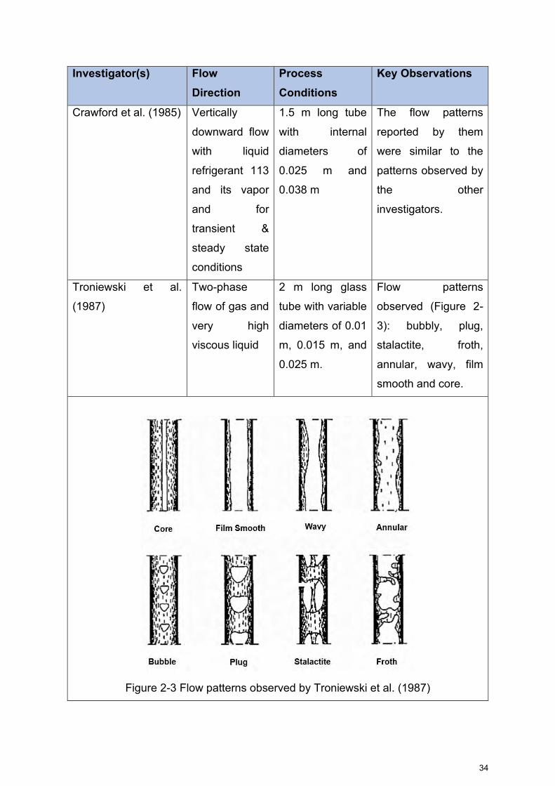
Troniewski et al.

(1987)

Two-phase

flow of gas and

very high

viscous liquid

2 m long glass

tube with variable

diameters of 0.01

m, 0.015 m, and

0.025 m.

Flow patterns

observed (Figure 2-

3): bubbly, plug,

stalactite, froth,

annular, wavy, film

smooth and core.

Figure 2-3 Flow patterns observed by Troniewski et al. (1987)

35

Investigator(s) Flow Direction

Process Conditions

Key Observations

Abdullah et al. (1994) Vertically

downward air-

water two-

phase flow

4 m long, 0.038

m diameter

perspex tube

Flow patterns

observed (Figure 2-

4): annular, slug, and

bubbly flow.

Figure 2-4 Flow pattern map by Abdullah et al. (1994)

Yijun et al. (1993) Vertically

downward flow

with air-water

0.0095 m

diameter tube

Flow patterns

observed: bubbly,

slug, froth, annular

and falling film.

Usui et al. (1989) &

Usui et al. (1983)

Vertically

downward two-

phase flow with

air-water, & U-

bends

Channels with

inside diameter of

0.016m, 0.024m,

0.032m and

0.038m

Flow patterns

observed (Figure 2-

5): bubbly, slug and

annular flows with

main focus to

estimate the average

void fraction and

transition criteria of

flow. For U-bends,

36

Investigator(s) Flow Direction

Process Conditions

Key Observations

similar flow patterns

are observed. In

addition, flow

separation is

observed for certain

conditions.

Figure 2-5 Flow patterns observed by Usui et al. (1989)

Bhagwat, (2011,

2012)

Vertically

downward two-

phase flow with

air-water

0.0127m

diameter poly-

carbonate tube

Flow patterns

observed (Figure 2-

6): bubbly, slug, froth,

falling film, annular

37

Investigator(s) Flow Direction

Process Conditions

Key Observations

Figure 2-6 Flow patterns observed by Swanand Bhagwat (2011, 2012)

Although, investigations on flow pattern maps are beyond the scope of current

investigations, it is prudent to have the knowledge of the flow pattern maps to provide

background necessary to enable the discussions at later stages. Interested readers

could get more details from earlier work carried out by various authors listed in above

section or in References including research carried by Spedding et al. (1999), Owen

et al. (1975), Ishii et al. (2004), Kashinsky et al. (1999), Coddington et al. (2002),

Barnea et al. (1982), Sekoguhi et al. (1996), Crawford et al (1985), Ishii et al. (2004,

2006).

2.2 Void Fraction and Void Fraction Correlations

The void fraction is one of the most important parameters used to characterize

the two-phase flows. It is the key physical value used to determine accurately the

parameters like two-phase density, two-phase viscosity, relative average velocity of

two-phases, and is of fundamental importance to predict the flow pattern transitions,

heat transfer and the two-phase flow pressure drop. Various geometric definitions are

used to specify the void fraction (John, 2001): local, chordal, cross-sectional and

volumetric. Several investigations are carried out earlier for upward flow and horizontal

two-phase flows (Melkamu et al., 2007; Butterworth, 1975 etc.). Only empirical void

38

fractions (based on experiments) and the correlations based on drift flux model related

to vertically downward flows are discussed in this section.

One of the oldest models to predict the void fraction is the drift flux model,

proposed by Zuber and Findlay (Kawanishi, 1990). The model is later modified by

several investigators including Wallis, Takashi et al. (2004). The drift flux model

considers the relative motion between the two-phases instead of the motion of the

individual phase. It is convenient to analyze the flow patterns that have strong

interaction between gravity, buoyancy, pressure and the two-phases itself. The

generalized two-phase flow drift flux model is represented by Equation 2-1.

𝜺 =𝑼𝒔𝒈

𝑪𝒐𝑼𝒎+𝑼𝒈𝒖 (2-1)

Where 휀 is the void fraction, Usg is the average superficial gas velocity, Um is the

mixture velocity. The most important parameters of the drift flux model are the

distribution parameter Co, which indicates the distribution of discrete phase (gas phase

generally) with reference to mixture in the pipe cross sectional area and the drift

velocity Ugu, which is the measure of the relative velocity of gas phase with reference

to mixture velocity.

For annular flow, Ishii et al. proposed using Equation 2-2 (John, 2001). The

later expression introduces the effect of liquid dynamic viscosity on void fraction. For

vertical downflow, the sign of ��𝑔𝑢 should be changed.

Co=1.0

��𝑔𝑢 = 23 [𝜇𝑙𝑈𝑙

𝜌𝑔𝑑𝑖] [

𝜌𝑙−𝜌𝑔

𝜌𝑙] (2-2)

Kawanishi et al. (1990) did extensive work with steam-water mixture and using

drift flux model for upward, downward flow and proposed empirical correlations with

large diameter tube. They used the drift velocity equation proposed by Ishii and given

by Equation 2-3.

��𝑔𝑢 = √2 [𝜎𝑔(𝜌𝑙−𝜌𝑔)

𝜌𝑙2 ]

1/4

(2-3)

39

The distribution parameter is given by Equation 2-4.

𝐶𝑜 = 0.9 + 0.1 (𝜌𝑔

𝜌𝑙)0.5

𝑓𝑜𝑟 0 > ��𝑔𝑢 > −2.5 𝑚/𝑠

𝐶𝑜 = 1.2 − 0.2 (𝜌𝑔

𝜌𝑙)0.5

𝑓𝑜𝑟 ��𝑔𝑢 < −3.5 𝑚/𝑠

𝐶𝑜 = 0.8 + 0.1 (𝜌𝑔

𝜌𝑙)0.5

− 0.3 [1 − (𝜌𝑔

𝜌𝑙)0.5

] (2.5 + ��𝑔𝑢) 𝑓𝑜𝑟 − 3.5 𝑚/𝑠 < ��𝑔𝑢 < −2.5 𝑚/𝑠

(2-4)

Yamazaki et al. (1978) developed a generalized correlation to determine the

void fraction leveraging Zuber’s drift flux model. They developed the correlation in

terms of void fraction and volumetric gas flow concentration (𝛽). Based on the data

from experiments, a correlation is developed. Equation 2-5 shows the general

correlation in upward flow.

(1− )(1−𝐾 )=

𝛽

1−𝛽(=

𝜌𝑙

𝜌𝑔.

𝑥

1−𝑥) (2-5)

And a simple equation for K is given by Equation 2-6.

𝐾 = 𝐾1 + 𝐾2𝛽𝑛 (2-6)

K1, K2 and n are experimental constants. The general correlation for void fraction,

independent of flow pattern, is then obtained by substituting Equation 2-6 into Equation

2-5. The three constants are estimated based on fitting of experimental data and is

given by Equation 2-7.

𝐾 = 2.0 −0.4

𝛽𝑓𝑜𝑟 𝛽 ≤ 0.2, 𝐾 = −0.25 + 1.25𝛽 𝑓𝑜𝑟 𝛽 ≥ 0.2 (2-7)

Usui et al. (1989) conducted experiments and found that the average void

fraction in downward flow highly depends on the flow regimes compared to that in

upward flow. The proposed correlations for bubbly and slug flow are based on drift flux

model. Based on their investigations, they observed that Co may approach 1.2 with

decreasing Eotvos number and the same is given by Equation 2-8, while the drift

velocity could be represented by Equation 2-9.

40

𝐶𝑜 = 1.2 −1

(2.95+350𝐸𝑜−1.8) (2-8)

𝑈𝑔𝑢 = 1.53[𝜎𝑔(𝜌𝑙 − 𝜌𝑔)/𝜌𝑙2]1/4 (2-9)

They proposed that the void fraction in slug flow can also be proposed by drift flux

model. The distribution parameter is found using the above equation and drift velocity

was calculated by using a relation given in Equation 2-10.

𝑈𝑔𝑢 = 𝐶1√𝑔𝐷(𝜌𝐿 − 𝜌𝐺)/𝜌𝐿 (2-10)

Where distribution parameter is given by Equation 2-11

𝐶1 = 0.345[1 − exp ((3.37 − 𝐸𝑜)/10)] (2-11)

They also proposed different void fraction correlations for annular flow and falling film

and are given by Equations 2-12 and 2-13.

(1 − 휀)23/7 − 2𝐶𝑤𝐹𝑟𝑙2 [1 ±

𝐶𝑖

𝐶𝑤

(1− )16/7

5/2

𝜌𝑔

𝜌𝑙(𝑢𝑔

𝑢𝑙)2

] = 0 (2-12)

휀 = 1 − (2𝐶𝑤𝐹𝑟𝑙2)7/23 (2-13)

Fr is the Froude number. They compared all these flow pattern dependent void fraction

correlations with their own experimental data and found a good agreement between

the estimated void fraction value and the experimental data.

Hibiki et al. (2004) did extensive work on two-fluid model with air-water system

and developed a correlation for void fraction and distribution parameter for downward

bubbly flow. They used the same drift velocity equation proposed by Ishii. The

distribution parameter is given by Equation 2-14.

𝐶𝑜 = (−0.0214(𝑗∗) + 0.772) + (0.0214(𝑗∗) + 0.228)√𝜌𝑔

𝜌𝑙 𝑓𝑜𝑟 − 20 ≤ 𝑗∗ ≤ 0

41

𝐶𝑜 = (0.2𝑒0.00848((𝑗∗)+20) + 1.0) − (0.2𝑒0.00848((𝑗∗)+20))√𝜌𝑔

𝜌𝑙 𝑓𝑜𝑟 𝑗∗ < −20 (2-14)

The equation for j* is given by following equation

𝑗∗ =𝑈𝑔

��𝑔𝑢

Based on their experimental work, they showed that the distribution parameter is

increased up to a certain value and gradually decreases and eventually approaches

to unity as the downward mixture volumetric flux is increased.

Sokolov et al. (1969) proposed a correlation that relates downward void fraction

to upward void fraction. The correlation is given by Equation 2-15.

휀𝑑𝑛 = 2𝛽 − 휀𝑢𝑝 (2-15)

Cai et al. (1997) analyzed the downward two-phase flow using air-oil fluid. They

proposed a model based on Zuber and Findlay drift flux model except the bubble rise

velocity assumes a negative sign since it is in the direction opposite to the flow

direction. They used their own experimental data to arrive at distribution parameter Co

and found that the distribution parameter for downflow is different from upflow and the

best fit line yielded Co=1.185. For slug flow, the Co value is found to be 1.15.

Clark et al. (1984, 1985) analyzed the Zuber and Findlay drift flux model for

both upflow and downflow. They performed experiments for air-water fluid combination

in a 0.1m ID pipe and performed regression using equation proposed by Wallis and

found that the bubble rise velocity is approximately equal to 0.25 m/s. The distribution

parameter Co = 1.165 gave the best fit for all data in bubbly flow for downflow and 1.07

for upflow.

Armand (1946) proposed a correlation and is given by Equation 2-16.

42

휀𝑑𝑛 =2 𝑢𝑝

𝐶𝐴− 휀𝑢𝑝 = 1.4휀𝑢𝑝 (2-16)

The CA is termed as Armand coefficient with a value of 0.83 and is applicable in the

region of low void fraction.

Yijun et al. (1993) performed experiments and proposed new correlations for

predicting the void fraction in vertical, gas-liquid, upward and downward two-phase

flow using a dimensional analysis approach. The void fraction is given by Equation 2-

17.

휀𝑑𝑛 = 0.076 + 0.074𝑅𝑒𝑙0.05휀𝑢𝑝 𝑓𝑜𝑟 𝑅𝑒𝑙 < 17400

휀𝑑𝑛 = 0.025 + 0.058𝑅𝑒𝑙0.05휀𝑢𝑝 𝑓𝑜𝑟 𝑅𝑒𝑙 > 17400 (2-17)

The Rel and Reg are the liquid and gas superficial Reynolds number denoted as,

𝑅𝑒𝑙 =𝜌𝑙𝑈𝑠𝑙𝐷

𝜇𝑙; 𝑅𝑒𝑔 =

𝜌𝑙𝑈𝑠𝑔𝐷

𝜇𝑔

The upward flow void fraction is given by Equation 2-18

𝛼𝑢𝑝

1−𝛼𝑢𝑝=

𝑥

1−𝑧𝑥 (2-18)

The z is determined by Equation 2-19.

𝑧 = 𝑅𝑒𝑙𝑛[𝑅𝑒𝑔𝐹𝑟𝑔

2]−𝑚 (2-19)

The values of the powers obtained are 0.95 and 0.332 for n and m respectively.

Bhagwat (2011, 2012) has done extensive work on analyzing the existing

correlations with his own experimental data. Based on his investigations, he concluded

that owing to the flexibility of the drift flux model, it is proved to be the most successful

43

model to predict the void fraction for downward flow. Based on the flow patterns, he

recommends the following correlations to be suitable. For the void fraction correlations

for specified ranges of the void fraction, he recommended the values presented in

Table 2-2. The correlations mentioned in Table 2-3 are recommended for flow pattern

independent void fraction correlations.

Table 2-2 : Recommended correlations for void fraction specified ranges (Bhagwat

(2011)).

Void Fraction Range

Correlation

0-0.25 Gomez et al. (2000) with Co = 1.15 𝑢𝑆𝐺

𝛼= (𝐶𝑜𝑈𝑀 + 𝑈𝐺𝑀𝑠𝑖𝑛𝜃(1 − 𝛼)0.5)0.076 + 0.074𝑅𝑒𝑙

0.05휀𝑢𝑝

0.25-0.50 Rouhani et al. (1970) – Use drift flux equation

𝐶𝑜 = 1 + 0.2(1 − 𝑥) (𝑔𝐷𝜌𝑙

2

𝐺2)

0.25

𝑈𝐺𝑀 = 1.18 (𝑔𝜎 [𝜌𝑙 − 𝜌𝑔

𝜌𝑙2 ])

0.25

0.50-0.75 Woldesemayat et al. (2007) – Use drift flux equation

𝑈𝐺𝑀 = 2.9(1.22 + 1.22𝑠𝑖𝑛𝜃)𝑃𝑎𝑡𝑚

𝑃 [𝑔𝐷𝜎(1 + 𝑐𝑜𝑠𝜃)(𝜌𝑙 − 𝜌𝑔)

𝜌𝑙2 ]

0.25

𝐶𝑜 =𝑈𝑠𝑔

𝑈𝑠𝑙 + 𝑈𝑠𝑔[1 + (

𝑈𝑠𝑙

𝑈𝑠𝑔)

𝜌𝑔

𝜌𝑙

0.1

]

0.75-1 Rouhani et al. (1970) – Use drift flux equation

𝐶𝑜 = 1 + 0.2(1 − 𝑥) (𝑔𝐷𝜌𝑙

2

𝐺2)

0.25

𝑈𝐺𝑀 = 1.18 (𝑔𝜎 [𝜌𝑙 − 𝜌𝑔

𝜌𝑙2 ])

0.25

44

Table 2-3 : Recommended correlations for flow pattern independent void fraction

correlations (Bhagwat (2011)).

No. Void fraction correlation 1 Cai et al. (1997) – Use drift flux equation

𝑈𝐺𝑀 = 1.53 (𝑔𝜎 [𝜌𝑙−𝜌𝑔

𝜌𝑙2 ])

0.25

for bubbly flow with Co = 1.185

𝑈𝐺𝑀 = 0.345√𝑔𝐷 (1 −𝜌𝑔

𝜌𝑙) for slug flow with Co = 1.15

2 Gomez et al. (2000) with Co = 1.15 𝑢𝑆𝐺

𝛼= (𝐶𝑜𝑈𝑀 + 𝑈𝐺𝑀𝑠𝑖𝑛𝜃(1 − 𝛼)0.5)0.076 + 0.074𝑅𝑒𝑙

0.05휀𝑢𝑝

3 Hasan (1995) – Use drift flux equation with Co = 1.12

𝑈𝐺𝑀,𝜃 = 𝑈𝐺𝑀√𝑠𝑖𝑛𝜃(1 + 𝑐𝑜𝑠𝜃)1.2

4 Nicklin et al. (1962) – Use drift flux equation with Co = 1.12

𝛼 =𝑈𝑆𝐺

𝐶𝑜𝑈𝑀 + 𝑈𝐺𝑀

Where 𝐶𝑜 = 1.2 𝑎𝑛𝑑 𝑈𝐺𝑀 = 0.35√𝑔𝐷

5 Rouhani et al. (1970) – Use drift flux equation

𝐶𝑜 = 1 + 0.2(1 − 𝑥) 𝑓𝑜𝑟 𝛼 < 0.25

𝐶𝑜 = 1 + 0.2(1 − 𝑥) (𝑔𝐷𝜌𝑙

2

𝐺2)

0.25

𝑓𝑜𝑟 𝛼 > 0.25

𝑈𝐺𝑀 = 1.18 (𝑔𝜎 [𝜌𝑙 − 𝜌𝑔

𝜌𝑙2 ])

0.25

More details on void fraction are provided in the references cited above. There

are a few more articles listed in the References section where the investigations on

void fraction are conducted by some of the previous researchers including Crawford

et al. (1985), Chexal (1986), Engineering data book by Wolverine etc. As described in

the first few paragraphs of this section, void fraction is one of the critical parameters

that would assist in determining the heat transfer and/or critical heat flux, which is the

area of interest of current research. Although, the void fraction determination is beyond

the scope of the current investigations, it enables the reader to read through the area

of interest of current research, which is critical heat flux. The next section discusses

about the critical heat flux.

45

2.3 Critical Heat Flux Critical heat flux (CHF) or burnout refers to the sudden decrease in the heat

transfer coefficient for a surface on which evaporation or boiling occurs. Exceeding

this heat flux causes the heat transfer surface to fill with vapor blanket instead of liquid.

This blanket acts like a barrier to heat flow from the heat dissipating device, resulting

in possible catastrophic failure of the device. The nuclear and conventional power

industries spend enormous amount of financial and human resources to understand

the CHF phenomenon and to establish appropriate margins and/or mitigation ways to

avoid the risk (Hall et al., 2000).

Several researchers extensively worked on developing CHF correlations for

horizontal and vertical up-flow conditions. One of the oldest and widely used

correlations is given by Zuber, termed as Zuber correlation. It was based on the

hydrodynamic stability analysis at water tube interface. A modified version of this

correlation is given in Equation 2-20 (Incropera et al., 2012). The void fraction used is

based on the homogeneous void fraction.

𝑞𝑚𝑎𝑥" = 0.149ℎ𝑓𝑔𝜌𝑣 [

𝜎𝑔(𝜌𝑙−𝜌𝑣)

𝜌𝑣2 ]

1

4[𝜌𝑙+𝜌𝑣

𝜌𝑙]

1

2(1 − 휀) [

𝐷8𝑚𝑚

𝐷]

1

2 (2-20)

Hall et al. (2000) did extensive work in collecting database for the work carried

out on CHF by several investigators. They developed their own correlation, covering

pressures up to 21.8 MPa (218 bar), tube diameters up to 44.7 mm, L/D ratio up to

684, mass flux up to 134 kg/m2s and heat flux up to 276 MW/m2. The correlation by

Hall et al. (2000) is given by Equation 2-21.

𝑞𝑚𝑎𝑥" = 𝐺ℎ𝑓𝑔0.0722𝑊𝑒−0.312 (

𝜌𝑙

𝜌𝑔)−0.644

[1 − 0.9 (𝜌𝑙

𝜌𝑔)0.724

(ℎ−ℎ𝑠𝑎𝑡,𝑜

ℎ𝑓𝑔)] (2-21)

Several correlations are developed for both horizontal flows and vertical up-

flows. Hall et al. (2000) compiled the data of the work carried out around the world on

CHF, covering a wide range of conditions and validated with lot of experimental data

(Katto et al. 1984; Shah 1987). However, to the best of the knowledge of the current

46

investigator, there is limited information available on critical heat flux available in open

literature for the vertically downward two-phase flows.

Papell et al. (1966) did extensive research with liquid nitrogen up to pressures

of 16.5 bar and for both vertically upward flows and vertically downward flows in a

round tube. They did not develop any explicit CHF correlation but their main

contribution is the maximum velocity of vapor bubble below which the buoyancy force

is found to be a dominant force resulting in vapor accumulation at the inlet and thereby

leading to two-phase flow instabilities and tube burnout. Blumenkrantz et al. (1968)

and Cumo et al. (1968) did a lot of research and concluded that the downflow CHF is

many times smaller than upflow CHF at low mass flow rates.

Sudo et al. (1985) studied the differences in departure for nucleate boiling

(DNB) heat flux between up-flow and down-flow in a vertical rectangular channel. They

considered 2 channels with dimensions 0.05 m width X 0.750 m in length X 0.00225

m flow gap and 0.05 m width X 0.375 m in length X 0.00228 m flow gap respectively.

The pressures considered up to 0.118 MPa (abs) [1.18 bar(a)], mass flux of 0-600

kg/m2s and inlet fluid temperature of 19-80oC. They mostly used air-water mixture as

working fluid and alloy600 plates are fixed along the width of the test section on either

sides for heating while the other side is not heated. Based on their investigations, they

found that the 𝑞𝐷𝑁𝐵" for downflow is almost same as that of upflow at very low G*

including zero and at high G* larger than about 300. At intermediate G* values of 1.5

to about 200, 𝑞𝐷𝑁𝐵" for downflow is much lower than the upflow. Another interesting

observation from their investigations is that the inlet sub-cooling of water is a key

parameter for the downflow at low G*, giving remarkably lower DNB heat flux with

lower inlet sub-cooling of water. Figures 2-7 and 2-8 show the effect of mass flux on

DNB for downflow based on their work (Sudo et al. 1985).

The non-dimensional G* is given by Equation 2-22.

𝐺∗ =𝐺

√𝐴𝑇𝑣(𝑇𝑙−𝑇𝑣)𝑔 (2-22)

47

Figure 2-7 Departure from nucleate boiling for downflow in a rectangular channel by

Sudo et al. (1985)

Mishima et al. (1985) studied the CHF at low mass velocities, flow stagnation

and flow reversal conditions by conducting experiments in a round tube with inner

diameter of 6 mm and at atmospheric conditions with water as working fluid. They

heated the test tube using a resistance heating method with copper electrodes placed

on either ends and supplied with the DC power. The main emphasis is given to

understand the effects of buoyancy, upstream compressibility and inlet valve throttling.

Some of the key contributions from their investigations are listed below.

Figure 2-8 Departure from nucleate boiling for downflow in various channels by Sudo

et al., (1985)

48

The stable flow CHF at low mass velocities can be well correlated by

conventional high-quality correlations such as Katto correlation. In downflow, the CHF

is as much as 30% lower than upflow at very low mass velocities due to the effect of

the buoyancy. The CHF at intermediate exit qualities appears to be significantly

affected by the density wave oscillations. Due to the buoyancy effect, the downflow is

less stable than upflow. At higher mass velocities, the flow direction shown minimal

impact. The CHF at low flow rate and low-pressure conditions is largely affected by

various flow instabilities. At lower heat flux, the basic mechanism of burnout is the dry-

out or breakdown of the liquid film on heated surface, caused by the deficiency of the

liquid in the heated section and may be controlled by such hydro-dynamical

phenomena as flooding or flow reversal, entrainment and deposition of liquid droplets.

Due to flow instabilities such as the density-wave oscillations, the pressure drop

oscillations and the flow excursion can reduce the effective film flow rate, thus leading

to the premature burnout of the tube.

Figure 2-9 shows the effect of inlet throttling on overall CHF behavior and for

both upflow and downflow. The curves are almost symmetrical about the zero mass

flux regions indicating that the buoyancy has negligible effect for upflow and downflow

in the presence of inlet throttling.

Figure 2-9 Effect of inlet throttling on overall CHF behavior (Upflow and Downflow) by

Mishima et al. (1985)

49

Figure 2-10 shows the effect of inlet plenum on the CHF for both upflow and

downflow. These investigations revealed that the effect of plenum is not significant in

upflow. However, the CHF drops to one-fifth in the absence of plenum for the downflow

indicating the significance of the plenum on the CHF for downflow. This could be

attributed to the destabilizing effect of the buoyancy and the upstream compressibility.

Figure 2-10 Overall behavior of CHF as a function of mass velocity for the test section

with upper and lower plenum in comparison with that for stiff system (Upflow and

Downflow by Mishima et al. (1985))

Chang et al. (1991) studied the CHF risk for very low flow of water in vertical

round tubes under low pressure conditions. They conducted the experiments for both

upflow and downflow scenarios and varying the inlet conditions like mass flux, sub-

cooling and throttling. They used stainless-steel (SS-304) tubes with inner diameters

of 6 mm and 8.8 mm, varied inlet fluid temperatures from 20oC to 70oC, mass flux in

the range of 6-187 kg/m2s and under atmospheric pressure conditions. They used the

DC power supply and resistance heating to heat the test section. Major conclusions

from their investigations are listed below:

Effect of mass flux: The CHF monotonously increases as the mass flux

increases from zero regardless of the flow direction and inlet throttling for stable

condition. Figure 2-11 shows the overall CHF as a function of mass flux. There

investigations also revealed that the CHF is almost symmetric about the line of zero

50

mass flux for both up flow and down flow for a stable system indicating that the effect

of buoyancy is almost negligible for a stable system. The U in the legend refers to up

flow and D refers to the down flow.

Figure 2-11 : Overall CHF behavior as a function of mass flux for stable flow

condition by Chang et al. (1991)

Effect of flow direction: When large inlet throttling is provided, the downflow

CHF is generally lower than the upflow CHF but the difference is not significant. On

the other hand, they found it almost impossible to maintain a stable downward flow

condition without inlet throttling indicating that the downward flow is much more

susceptible to the instabilities and premature CHF due to flow excursion can occur in

downflow if such instabilities are not effectively suppressed. Figure 2-12 shows the

effect of flow direction on CHF. The U in the legend refers to up flow and D refers to

down flow.

Effect of inlet throttling: Throttling just before the inlet of a boiling channel under

low pressure increases the stability of flow, and therefore generally increases the CHF

and is dominant for downflow conditions. Figure 2-13 shows the effect of inlet throttling

on CHF. The effect of inlet throttling on CHF at very low flow region is almost negligible.

The authors also found that they were unable to maintain a stable flow without the

throttling for downward flows. They did not report out the downward flow trends with

and without throttling.

51

Effect of inlet sub-cooling: The effect of inlet sub-cooling is small and obscure

in the stable low flow conditions under low pressure. Authors were unable to perform

experiments beyond certain mass flux although they had some indications of effect

of inlet subcooling above 190 kg/m2s.

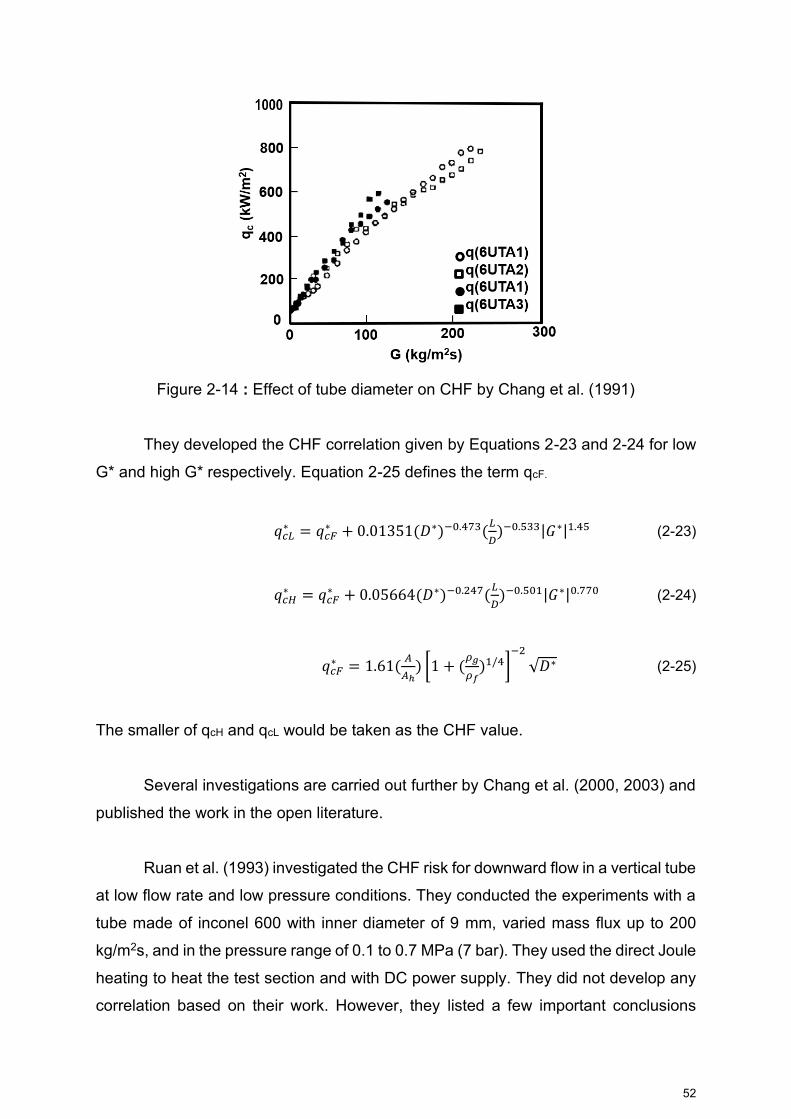
Effect of tube diameter: The large diameter tube gives a higher CHF and a lower

critical quality as expected. This is for a fixed set of inlet conditions. Figure 2-14 shows

the effect of tube diameter on CHF. All the results were reported out for the vertically

upward flows with hardly any information presented for vertically downward two-phase

flows.

Figure 2-12 : Effect of flow direction on CHF by Chang et al. (1991)

Figure 2-13 : Effect of inlet throttling on CHF by Chang et al. (1991)

52

Figure 2-14 : Effect of tube diameter on CHF by Chang et al. (1991)

They developed the CHF correlation given by Equations 2-23 and 2-24 for low

G* and high G* respectively. Equation 2-25 defines the term qcF.

𝑞𝑐𝐿∗ = 𝑞𝑐𝐹

∗ + 0.01351(𝐷∗)−0.473(𝐿

𝐷)−0.533|𝐺∗|1.45 (2-23)

𝑞𝑐𝐻∗ = 𝑞𝑐𝐹

∗ + 0.05664(𝐷∗)−0.247(𝐿

𝐷)−0.501|𝐺∗|0.770 (2-24)

𝑞𝑐𝐹∗ = 1.61(

𝐴

𝐴ℎ) [1 + (

𝜌𝑔

𝜌𝑓)1/4]

−2

√𝐷∗ (2-25)

The smaller of qcH and qcL would be taken as the CHF value.

Several investigations are carried out further by Chang et al. (2000, 2003) and

published the work in the open literature.

Ruan et al. (1993) investigated the CHF risk for downward flow in a vertical tube

at low flow rate and low pressure conditions. They conducted the experiments with a

tube made of inconel 600 with inner diameter of 9 mm, varied mass flux up to 200

kg/m2s, and in the pressure range of 0.1 to 0.7 MPa (7 bar). They used the direct Joule

heating to heat the test section and with DC power supply. They did not develop any

correlation based on their work. However, they listed a few important conclusions

53

based on their investigations. They observed two different kinds of CHF behavior. The

first one is characterized by the periodic wall temperature pulsation of great amplitude

along almost the entire test section, with vapor reaching the upper end of the heated

length. This unstable boiling crisis is related to the sustained flow instability of the

alternate occurrence of the co-current downward flow and countercurrent flow in the

bubbly or slug flow, caused by the combined effect of the upstream compressibility

and the buoyancy acting on the bubbles opposed to the flow direction. They termed

this as flooding type CHF. The second one is characterized by the wall temperature

excursion at the exit of the test section and can be interpreted as dryout in annular

flow and termed as CHF2.

Figure 2-15 shows the relation between inlet sub-cooling and occurrence of

CHF1 and CHF2. The key observation is that the CHF1 occurred not only at high but

also at low inlet sub-cooling. Before its occurrence, the inlet sub-cooling began to

decrease. The same trend is not observed for CHF2.

Figure 2-15 : Relation between inlet sub-cooling and occurrence of CHF1 and CHF2

by Ruan et al. (1993)

Based on their investigations they identified certain characteristics for the CHF

of downward flow. Figure 2-16 shows the variation of CHF characteristics with inlet

sub-cooling. They found that the effect of inlet sub-cooling is profound especially for

the case with upstream compressibility. This is due to the fact that the CHF value

would abruptly jump to a much higher level as the inlet sub-cooling decreases to a low

54

value at which the inlet water is nearly saturated. Except for this, they did not find the

dependency of CHF on the inlet sub-cooling, especially at the low mass flow rates

under elevated pressures.

Figure 2-16 : Variation of CHF characteristics with inlet sub-cooling (at CHF) by

Ruan et al. (1993).

Figures 2-17, 2-18 show the variation of CHF with pressure. The effect of

pressure on downward flow is significant with obvious increase in CHF due to increase

in pressure except for the case of large upper plenum. The reason is due to increase

in vapor to liquid specific volume ratio, resulting in smaller bubbles along with the

upstream compressibility. This implies the flow becomes more stable at elevated

pressure conditions. They also compared the flooding type CHF (CHF1) correlation

with the correlation proposed by Mishima et al. and between the stable flow CHF

(CHF2) with the correlation proposed by Weber for the stable upflow CHF. They found

that the data is in good agreement and concluded to propose these two correlations

as the lower and upper limits for the CHF for downward flow in vertical tube at low flow

rate and low-pressure conditions.

Mishima et al. (1987) investigated the effect of channel geometry on CHF for

low pressure water and for both upflow and downflow conditions. They conducted the

experiments in annulus, rectangular ducts and round channels at pressures close to

atmosphere. For downflows in rectangular channels, burnout occurs due to flooding

at low mass velocities less than the critical value to stagnate steam bubbles in the

55

heated channel. The resultant CHF is at minimum. The critical mass velocity for bubble

stagnation is calculated based upon the drift flux model given by Ishii. At intermediate

mass velocities beyond the critical mass velocity, burnout occurs at about zero exit

quality. In this region, vigorous flow oscillations arise, whose amplitude increases with

increasing mass velocity and heat flux. For round tubes, they found that for the stiff

system, the CHF is as much as 30% lower than the upflow high quality CHF at very

low flow rates; however, the difference disappears as the flow rate increases. At

intermediate mass velocities, there is a region where the CHF is almost constant as a

function of mass velocity, as is the case in upflow. The CHF is lower as the flow

becomes less stable. At sufficiently high mass velocities, burnout occurs due to flow

excursion.

Figure 2-17 Variation of CHF characteristic with mass flow rate at atmospheric

pressure by Ruan et al. (1993)

Figure 2-18 Variation of CHF characteristics with mass flow rate at elevated pressure

condition by Ruan et al. (1993)

56

Sudo et al. (1989) developed a CHF correlation for downward flow in a narrow

vertical rectangular channel heated with plates fixed on both sides of the width of the

channel. They conducted experiments for the countercurrent flow scenario wherein

the water travels downwards while the air travels upwards. They conducted

experiments at pressure of 1 atm with an inlet sub-cooling range of 25-75K, inlet mass

flux range of 2600 kg/m2s and in 2.25 mm and 2.80 mm gap flow channels, heated

from both sides. They developed a correlation given by Equation 2-26. The definition

of terms F and Bond number are given by Equations 2-27 and 2-28 respectively.

𝑞𝐶𝐻𝐹∗ =

𝐴

𝐴𝐻[(

𝐶𝑝Δ𝑇𝑠𝑢𝑏

ℎ𝑙𝑔)𝐺∗ + (

1

1.52)2

(𝑎

𝜆)0.5

𝐹2.875] (2-26)

𝐹 = 1.30.7 − [1.52 (𝜆𝜌𝑔

𝑎𝜌𝑙)0.25

(0.5 + 0.0015𝐵𝑜1.3)𝐺∗0.5]0.7

(2-27)

𝐵𝑜 =𝑎.𝑏(𝜌𝑙−𝜌𝑔)𝑔

𝜎 (2-28)

G* is given by equation 2-29

𝐺∗ =𝜌𝑙𝑗𝑙𝑖

√𝜆𝜌𝑔(𝜌𝑙−𝜌𝑔)𝑔 (2-29)

They also referred to the CHF correlation for downward flow given by Mishima given

by Equation 2-30.

𝑞𝐶𝐻𝐹∗ =

𝐴

𝐴𝐻(𝐶𝑝Δ𝑇𝑠𝑢𝑏

ℎ𝑙𝑔)𝐺∗ + 𝐶2 (

𝐴

𝐴𝐻)

√𝑎

𝜆

[1+𝑚(𝜌𝑔

𝜌𝑙)1/4

]

2 (2-30)

The term λ is defined by Equation 2-31.

𝜆 = [𝜎

𝑔(𝜌𝑙−𝜌𝑔)]1/2

(2-31)

Figure 2-19 shows the experimental results of CHF versus G* for downward

flow in a vertical rectangular channel. At higher inlet water Sub-cooling ΔTsub gives a

57

higher CHF. A shorter heated length also gives a higher CHF. For G*>20, a larger G*

gives a higher CHF. In the case of ΔTsub = 25K, the CHF becomes a minimum for G*

= 20; while in case of ΔTsub = 75K, the CHF becomes a minimum for G* = 2.0 under

the flooding conditions.

Their main contribution includes developing a new CHF prediction for

downward flow in vertical rectangular channels based on new CCFL correlation. The

proposed correlation shows much better coincidence with the experimental results

than the prediction based on the existing flooding correlation, making clear the

undetermined role of the aspect ratio of rectangular channel. They concluded that the

CHF for downward flow is minimum under the flooding condition in the case of large

inlet water sub-cooling and for the case with large inlet downward water mass flux

when compared to the flooding condition with small inlet water sub-cooling.

Takeyuki et al. (2015) conducted experiments to understand the influence of

the diameter of the tubes on the CHF in vertically downward flows. They compared

the results with the data from the upward flow experiments conducted in addition to

the experiments conducted for vertically downward two-phase flows. Based on their

investigations, they revealed that the experimental CHF could be classified into four

types. The four types are due to complete dryout of falling liquid film, flooding, hydraulic

instability, and liquid film dryout in annular flow. The CHF could arise due to one of the

four types described above and driven by the pressure drop, location of CHF, and inlet

degree of sub-cooling. Yoshiki et al. (2018) conducted experiments to understand the

CHF caused by the hydraulic instability. They formulated the CHF for hydraulic

instability type by two different models. For low flow rates, they found that the Kelvin

Helmholtz instability model would be suitable. For high mass fluxes, they proposed a

modified model of the departure from nucleate boiling (DNB). They concluded that

these predicted models show good agreement with the experimental data. Kohei et al.

(2018) studied the liquid film amount at the condition of critical heat flux for vertically

downward flow by using liquid film extraction method. They conducted the experiments

in lot of test sections by varying lengths and proposed the modifications to Koizuimi

correlation. They also concluded that the results show better qualitative trends but

differences exist quantitatively and linked the differences to the basic flow structure of

downward flow when compared to upward flow.

58

Figure 2-19 : Comparison of CHF versus G* by Sudo et al. (1989)

Shen et al. (2014) conducted experiments to understand the heat transfer

characteristics of smooth tube with downward flow. They conducted the experiments

by varying pressures from 11.5 MPa (115 bar), mass flux rates from 450 to 1550

kg/m2s and heat flux on inner wall from 50 to 585 kW/m2. The effect of heat flux on

heat transfer coefficient and wall temperature is analyzed and the corresponding

empirical correlations are presented by them. The heat transfer coefficients of

downward flow are compared with that of vertical upward flow. The results show that

at sub critical and near critical pressure, dryout and departure from nucleate boiling

can occur in vertical downward tube. With the increase of heat flux, heat transfer

deterioration occurs ahead and the peak wall temperature after heat transfer

deterioration increases. At supercritical pressure, the wall temperature increases

slowly with fluid enthalpy when the bulk temperature is lower than the pseudo-critical

temperature and increases considerably when the bulk temperature is higher than the

pseudo-critical temperature. In the pseudo-critical enthalpy region, the heat transfer is

enhanced. Figures 2-20, 2-21, 2-22 shows the comparison of wall temperatures of

vertical downward tube and vertical upward tube at sub-critical pressure, near critical

pressure and super-critical pressure respectively.

Aroonrat et al. (2013) conducted experiments in corrugated tubes with flow

directed vertically downwards. The main emphasis is given on understanding the

pressure drop and the evaporative heat transfer of refrigerant R-134a by varying the

pitch of the corrugation. They concluded that the heat transfer coefficient and the

59

frictional drop are higher in corrugated tubes when compared with the experiments

conducted in smooth tubes. Mohammed et al. (2008) conducted experiments in

vertically upward and downward flows in circular cylinders to understand the mixed

convection heat transfer for laminar flows. They reported that the surface values are

higher for flows directed downwards when compared to flows directed upwards but

are lower than the horizontal flows.

Figure 2-20 : Comparison of wall temperatures for vertically upward and vertically downward flow at 18 MPa pressure by Shen et al. (2014)

Figure 2-21 : Comparison of wall temperatures for vertically upward and vertically downward flow at 20.5 MPa pressure by Shen et al. (2014)

60

Figure 2-22 : Comparison of wall temperatures for vertically upward and vertically downward flow at 28 MPa pressure by Shen at al. (2014)

Rajeshwar et al. (2017) compiled the CHF correlations and heat transfer

coefficient investigations available for vertically downward flows. Some of the recent

investigations focused on understanding the bubble dynamics in vertically downward

two-phase flows. Atul et al. (2019) conducted experiments in vertically upward and

vertically downward two-phase flows to understand the thermal impact and the

dynamics of vapor bubble. They visualized the growth of the bubble, studied the

detachment of the bubble from the heater surface and investigated the differences in

the bubble trajectory after departure from the nucleation site for both the flow

configurations. They observed significant differences in the bubble trajectory between

the vertically upward and vertically downward two-phase flows. Their work also

indicates the interest in the researchers to investigate the flow dynamics and the heat

transfer phenomenon in the vertically downward two-phase flows and continues to be

one of the interesting areas for research.

There were lot many investigations carried on understanding the CHF and

which forms the basis for the subsequent investigations on CHF. For instance, the

work carried out by Levy (1962), Kakac (2008, 2010), Biasi (1967) is still being used

by most of the investigators. A few of the investigations carried out on CHF are listed

in References and are reviewed during the current investigations.

61

2.4 Numerical Modeling

The major focus of the current investigations is to determine the CHF for

vertically downward two-phase flows experimentally. However, a few investigations

are also carried out using numerical computational fluid dynamics (CFD) tools. These

investigations are carried out to understand the boiling models available in open

commercial CFD software that could be applicable to simulate the vertically downward

two-phase flows and thereby optimize the test rig design and/or reduce the number of

experiments. Prior art search is conducted to understand the available numerical

models for boiling in open literature and is discussed below.

Huiying Li et al. (2011) developed a numerical model to predict the boiling and

critical heat flux using a Eulerian multiphase boiling model. They developed the

models in conjunction with the wall boiling models (Rensselaer Polytechnic Institute

(RPI) boiling model in Fluent) for nucleate modeling. The critical heat flux and the non-

equilibrium wall functions are modeled by extending the RPI model to departure from

nucleate boiling (DNB) by splitting the wall heat flux to both the liquid and vapor

phases. They validated the numerical models with the experimental data at high

pressures. Apart from developing the models and validating them, importance is also

given to the grid sensitivity investigations, turbulence models and other critical

parameters in their investigations.

Ribeiro et al. (2017) conducted analysis of sub-cooled flow boiling in vertically

upward two-phase flow subjected to high pressure using CFD. The inner diameter of

the tube considered for simulations is 0.00154m, pressure considered is 4.5 MPa (45

bar) and water mass flux is 900 kg/m2s. The numerical results are validated with the

experimental data reported by Bartolomei et al. (1967), with emphasis given on the

wall temperature, liquid bulk temperature and the location of the departure of nucleate

boiling. The results showed that the numerical results are in good agreement with the

plant data for the parameters listed above. Grid independent studies revealed that the

results are less impacted with the grid except for the convergence difficulties. Figures

2-23 and 2-24 show the wall temperature predictions and the void fraction using four

different interfacial heat transfer models studied by them in their investigations and

comparison with the experimental data.

62

Figure 2-23 : Comparison of wall temperatures of 4 interfacial heat transfer models

with the experimental data; chart by Ribiero et al. (2017)

Naveen et al. (2017) investigated the boiling models using numerical code

Fluent by ANSYS Inc. with sodium as working fluid. They validated their numerical

models with Bartolomei et al. (1967) for pressurized water simulations and refrigerant

R12 with DEBORA experiments (Garnier et al., 2001). Both these investigations are

carried out at 45 bar and 30.06 bar respectively. The numerical results showed are in

good agreement with the experimental data at such high pressures.

Figure 2-24 : Comparison of void fraction of different interfacial heat transfer models

with the experimental data; chart by Ribiero et al. (2017)

Figure 2-25 shows the void fraction, liquid temperature and wall temperature

predictions along the axial length for the pressurized water case compared with the

63

experimental data. Grid sensitivity results are also included based on their

investigations.

Figure 2-25 : Comparison of pressurized water boiling numerical results with

experimental data; chart by Naveen et al. (2017).

Figure 2-26 shows the comparison of the void fraction, vapor velocity and the

bubble diameter for the R12 numerical modeling case with the experimental data. The

results are shown for different grid sizes. The results for both pressurized water and

the R12 case showed good agreement with the experimental data. Further, they

indicated that the bubble diameter exhibited a larger deviation with experimental data,

especially for R12 case. When they invoked bubble coalescence and breakup model,

the bubble diameter approached the experimental value.

They extended the simulation to investigate sodium at atmospheric pressure

and found that the solution showed a pulsating boiling behavior with periodic bubble

formation, growth and collapse occurring.

64

Figure 2-26 : Comparison of R12 boiling numerical results with experimental data;

chart by Naveen et al. (2017).

Vyscosil et al. (2008) documented their numerical results generated using

NEPTUNE_V2 CFD and Fluent CFD codes with refrigerant R12 at high pressure in

vertically upward two-phase flows and validated with the numerical experiments by

DEBORA. They concluded that both the model results are comparable and are in good

agreement with the experimental data.

Hemanth et al. (2013) conducted numerical simulations using ANSYS Fluent to

simulate the subcooled nucleate boiling in cooling jacket of an IC engine. The fluid

used was ethylene glycol. The results are compared with the experimental results and

are found in good agreement.

Sumanth et al. (2018) performed numerical simulations using Fluent CFD code

for vertically downward flows. They validated the existing models to predict void

fraction, wall temperature and CHF in upward flows with the experimental data in open

literature and extended the validated models to simulate vertically downward flows at

high pressures and high mass fluxes. They concluded that at high pressures and high

65

mass fluxes, the numerical simulations show hardly any difference between upward

flow and downward flow indicating the minimal impact of flow direction at these

conditions. Figure 2-27 shows the comparison of CHF in upward and downward flow

based on their numerical simulations. However, they did not comment about the

applicability of these models for vertically downward two-phase flows at low pressures

and low mass fluxes.

Figure 2-27 : Comparison of wall temperature from numerical simulations for upward

and downward flow at high pressure and high mass flux conditions by Sumanth et al.

(2018)

Rajeshwar et al. (2019) conducted numerical simulations for both vertically

upward and vertically downward flows covering the pressure range from 7.01 MPa

(70.1 bar) to 0.1 MPa (atmospheric pressure). They conducted simulations for a range

of mass fluxes, heat fluxes and inlet sub-cooling to understand the pressures at which

the code tends to diverge. Based on their investigations, it is found that at pressures

in the range of 1 MPa (10 bar) to 1.5 MPa (15 bar) is the pressure below which the

code diverges and recommends suitable sensitivity analysis to be carried out to come

up with convergence strategies.

While there are many articles available in open literature on boiling models, the

discussion is restricted to a few articles as the main emphasis of the current

investigations is experimentation.

66

2.5 Literature Search Summary

Comprehensive literature search is conducted to understand the critical heat

flux correlations and the heat transfer characteristics for a vertically downward two-

phase flow. Most of the previous investigations focused mainly on understanding the

flow pattern maps and the development of void fraction correlations. This section

summarizes the investigations carried out by the previous investigators on vertically

downward two-phase flow.

Significant work is done previously on vertical downward two-phase flows,

especially to understand the flow pattern maps and developing void fraction

correlations. The experimental work carried out by the authors observed coring bubbly,

bubbly-slug, falling film, froth, and annular flow patterns. They also observed a peculiar

flow pattern termed as wetted wall flow pattern. Some authors also found a different

flow pattern termed as core and stalactite flows. There are only a limited number of

void fraction correlations available exclusively for downward two-phase flow in

comparison to upward two-phase flows. Most of the earlier work is carried out at

relatively low pressures. Majority of the void fraction correlations are developed based

on drift flux model and are dependent on the type of flow patterns. Only a few

researchers compared their experimental data with the correlations developed by the

other researchers. In addition, the information on comparison of the correlations over

a wide range of operating conditions is limited.

There is limited work carried out on understanding the CHF for vertically

downward two-phase flows experimentally and hardly any work carried out

numerically. The literature search conducted as part of these investigations reveals

the following:

1. Most of the previous investigations on CHF are conducted at atmospheric

pressure, where the potential risks of tube failure are significantly high. This is

attributed by the large density differences between gas and liquid phase,

resulting in more vapor accumulation at the top and thereby leading to two-

phase flow instabilities and/or premature tube burnout. However, most of the

boilers and heat exchangers in the power and chemical industries operate at

67

much higher pressures. The information at such high pressures for vertically

downward two-phase flows is limited.

2. In contrast to the number of CHF correlations available for vertically upward

two-phase flows and horizontal flows, there are hardly any CHF correlations

available for vertically downward flows. The CHF correlations for vertically

upward and horizontal flows cover wide range of process or operating

conditions while the same for vertically downward flows covers mostly at

atmospheric condition.

3. Previous investigators used air-water mixture, water-steam mixture,

refrigerants to assess the CHF for vertically downward two-phase flows.

However, the investigations carried out with water-steam mixture and reports

from these investigations are limited for vertically downward two-phase flows.

The other important area where the information is hardly available if for the

cryogenic liquids.

4. Inlet throttling and inlet plenum are two major aspects that could enhance the

magnitude of CHF and thereby reduces the risk significantly. Most of the

previous investigations on the CHF for vertically downward two-phase flows

included the effect of inlet throttling or inlet plenum. The correlations developed

also included the effects of inlet throttling and the inlet plenum. However, the

published research on vertically downward two-phase flows in the absence of

the inlet throttling or inlet plenum is limited. While CHF measured or estimated

with inlet throttling or plenum could be considered to be the upper bound for

CHF, the absence of these influencing parameters could be considered as

lower bound. Establishing these limits is critical from equipment operation

perspective and hence is of greater importance.

5. Importance is also given to the geometry of the test section. Most of the

investigations focused on using a rectangular channel as the test section. There

are a few investigations reported based on round tubes and annulus tubes.

6. One of the parameters that could influence the boiling phenomenon inside the

tube is the uniformity of the heating all along the test section. Previous

investigations mostly used resistance heating using DC power supply to heat

the test section. Electrodes are connected on either ends of the test section.

While this method of heating strongly depends on the resistivity of the test

material. The variation in resistivity due to change in temperature is ignored by

68

most of the researchers and assumed uniform heating. On the other hand, as

most of the investigations used rectangular channels as test section in which

plate heating is used to heat the test section. The heating plates are attached

to the rectangular channels on wider surface while the narrower surfaces are

ignored. The previous investigators did not specifically discuss about the impact

of ignoring these narrower surfaces on the overall CHF predictions.

7. Some of the investigations carried out to understand the CHF primarily focused

on the tube diameters but they did not develop any explicit CHF correlations. A

few investigators conducted experiments to understand the bubble dynamics in

vertically downward flows and restricted their investigations to the bubble

dynamics.

8. There are a few investigations carried at sub-critical pressures for vertically

downward two-phase flows. However, these investigations mainly focused on

understanding the heat transfer coefficient trends and comparison of these heat

transfer coefficient values with the vertically upward two-phase flows. Some of

the authors investigated the influence of corrugation on the heat transfer

coefficient and compared the same with the plain tubes but did not specifically

talk about the CHF.

9. Most of the previous numerical investigations using the existing boiling models

are validated with the experimental data at high pressures and for vertically

upward flows. Not many investigations are reported out for vertically downward

flows.

10. The previous numerical investigations carried out on vertically upward flows are

conducted at high pressures. There are hardly any investigations reported out

at atmospheric pressures.

11. Further, there is no CHF correlation developed using vertically downward flows

and compare the same with the CHF correlation in open literature based on

experiments.

As it is evident from the above discussion, previous investigations on CHF for vertically

downward two-phase flows provided good insights on the risks and at the same time

provided opportunities to explore a lot in this field. This forms the motivation for the

current investigations and set the tone for rest of the chapters.

69

Chapter 3 Problem Definition

The detailed literature search carried out on vertically downward two-phase

flows revealed that the CHF information is limited in comparison to the abundant data

available for vertically upward two-phase flows and horizontal flows. In addition to the

data on CHF, some of the key observations from the previous investigations and the

limitations associated with the vertically downward two-phase flows provided an

opportunity to explore this field further. One of the areas that require attention is to

develop a CHF database for vertically downward two-phase flows in similar lines to

the CHF database available for vertically upward two-phase flows, covering wide

range of operating conditions. One of the pre-requisites to develop such database is

to improve the existing CHF correlations for vertically downward two-phase flows by

extending the range of its applicability, especially in terms of pressure. The current

CHF correlations available for vertically downward two-phase flows are mostly

developed at atmospheric pressure conditions. The main objective of the current

investigations is to develop a CHF correlation by including the pressure effects beyond

the atmospheric pressure. The plan is to build an experimental test rig that could be

used to determine the CHF by operating at pressures above the atmospheric pressure.

The presence of inlet throttling, inlet plenum or other CHF magnitude enhancing

mechanisms would abruptly increase the CHF magnitude and thereby reduces the

risks associated with CHF significantly. Absence of these CHF enhancing

mechanisms would define the lower bounds where the risk is supposed to be

significantly high and thereby constituting the worst scenario. The idea of the current

investigations is to determine the lower bound of CHF by possible elimination of such

CHF enhancers for vertically downward two-phase flows. Based on the observations

from previous investigations and as summarized at the end of the previous chapter,

there is a scope to improve a few areas for the accurate prediction of CHF for vertically

downward two-phase flows. The current investigations aim at improving the CHF

predictions by including a few design modifications that could enhance the accuracy

of the predictions. Experimental investigations are time consuming, cost extensive and

involves high risk factors especially from human safety. Inclusion of high pressure and

high temperature steam makes it even more challenging. The advancements in the

computational resources makes the numerical modeling a viable option to mimic some

70

of the experimental test runs. However, the limitations in the numerical models for

boiling problems makes it challenging, especially from convergence perspective and

at low pressures. With no significant data reported out from numerical simulations

earlier on vertically downward two-phase flows, it gives an opportunity to explore this

area further. The validated numerical models could eventually reduce the number of

experimental runs and thereby save money, time and most importantly reduces the

risks associated with safety. The second main objective of the current investigations

is to explore the numerical models available commercially and check for its

applicability for the vertically downward two-phase flows. In addition, a validated CFD

model might also provide an opportunity to develop a CHF correlation covering a wide

range of process conditions and thereby reducing the number of experimentations

significantly.

In a nutshell, the present study focuses on investigating the CHF in a vertically

downward two-phase flow using water as working fluid. Design, development and

commissioning of an experimental test rig is one of the key activities as part of these

investigations. All the investigations are carried out at low pressures to moderate

pressures and generalized correlation is developed /checked, by including pressure,

throughput, inlet fluid temperature and other parameters, which could impact the

critical heat flux. The investigations are extended by using numerical tools available

commercially in open market and develop the CHF correlation using the validated

numerical tool and provide suitable recommendations.

The following list of items would define the scope of the current investigations.

The out of scope items are also listed to ensure the activities that would not be included

as part of the current investigations and could form the basis for the future scope of

work.

3.1 In Scope

• Design and development of test rig to conduct CHF experiments in vertically

downward two-phase flows at elevated pressures up to 5bar.

71

• Summary of risk assessment/ failure mode analysis/ safety analysis carried out

to develop the test rig.

• Calibration of the instruments used in the current experiments and validating

with available open literature data

• Detailed description of proving runs, development of test matrix to conduct

experiments, experiments and observations from the current experiments.

• CHF correlation development and uncertainty analysis.

• Numerical modeling using CFD commercial software Fluent by ANSYS Inc.

Brief discussion on available boiling models etc. in Fluent. Validation of

numerical models and applicability to current numerical investigations.

Development of CHF correlation using numerical tools and comparing it with

experimental data.

3.2 Out of Scope

• Investigation on flow pattern maps/ development of void fraction correlation.

• Extensive investigations on two-phase flow pressure drops.

• Investigation on inclusion of foreign particles and its impact on CHF.

• Water chemistry and its impact on CHF.

• System level instabilities and its investigation.

• Characteristics of pumps and other piping equipment used and its impact on

CHF.

• Investigation with different working fluids except water.

• Development of numerical models and/or codes (user defined functions) for the

boiling models.

72

Chapter 4 Experimental Work The main objective of the current investigations as listed in the previous chapter

is to design, develop and commission an experimental test rig, followed by conducting

experiments at pressures ranging from atmospheric to moderate pressures. The end

objective is to develop a CHF correlation as a function of listed variables, which will be

discussed in the next chapter. This chapter discusses about the experimental work

carried out as part of these investigations. The discussion focusses on the design and

development of the test rig. Some of the key design improvements made based on the

observations from the previous investigations are discussed. The details of the

instruments used and the calibration procedures adopted are also discussed to a

greater extent. Safety is never compromised during the entire experimentation phase

including design, development, commissioning, experimentation and validation. Some

of the key safety related aspects are also discussed to the extent required in this

chapter.

The experimental test rig is commissioned with the support of MVGR College

of Engineering, Chintalavalasa, Vizianagaram, India. The college has provided the

premises to setup the test rig, supplied basic amenities like electricity, water and the

skilled workers for assembling the test rig and to attend minor repairs, if any. This is

over and above the technical sessions that faculty has participated during the design,

commissioning and experimentation phases.

Figure 4-1 shows the experimental test rig that is built as part of current

investigations. The main components of the test rig are:

1. Reservoir/ water storage tank

2. Reservoir/ water storage tank

3. Pump

4. Heater section/ test section

5. Variacs/ Variable transformers

6. Display units with temperature indicators (hidden behind the variacs)

7. Piping network

a. Pipe b. Test pipe c. Valves

73

d. Elbows, tees, bends and couplings 8. Instrumentation

a. Temperature gauges (Quantity: 4, only one is highlighted for reference) b. Pressure gauges (Quantity: 3, only one is highlighted for reference c. Flow meter (Quantity: 1) d. Thermocouples (Quantity: 16, only one is highlighted for reference)

Figure 4-1: Experimental test rig

A few auxiliary equipment is also used for setting up this test rig and are not

listed. All the individual components are bought as separate entities and assemble at

the site. The next section discusses about the details of the test rig.

Reservoir/ Water Tank:

Reservoir/ water tanks are the storage tanks that are used to store the water

for current investigations. A total of 2 reservoirs are used for the experiments. Both

these reservoirs are fabricated within the premises of the college. The material of

construction of these reservoirs is galvanized iron. The shape is achieved by welding

a 3.5 mm thick plates with a compatible weld filling rod. A leak test is conducted for

74

individual reservoirs post welding. The tanks are filled with water and retained for a

day to check for drop in the liquid levels. Visual inspection is also done to check for

the leakages. These reservoirs are coated with zinc coating followed by corrosive

resistant paint. The first reservoir capacity is ~250 L while the second reservoir

capacity is ~200 L.

From the functionality perspective, the first reservoir receives water from the

main source, and supplies water to the test section using a pump during the

experiment. A bypass line is in place and directs the water back to the reservoir in

order to meet the flow requirements during the experiment. The return line is also

directed to this tank to complete the water circuit. The second reservoir is used while

conducting the experiments. The high pressure, high temperature steam coming from

the test section is directed into the second reservoir. The second reservoir is pre-filled

with cold water. The steam and steam/mixture water from the test section is introduced

into the second reservoir through a pipe that is extended from top to almost the bottom.

This is done to ensure that the steam would be in contact with water for sufficient time

and gets condensed. The second tank is closed from the top and could be opened up

easily. The first tank is open to atmosphere. However, the actual flow measurement is

taken in the second reservoir during the experimentation and steam condensation

aspects are not considered except for a few cases.

Pump:

As the experiments are conducted at relatively high pressure and high

temperatures, a high-end pump is chosen for the experiments. The pump is

manufactured by GRUNDFOS Inc. and is imported from Denmark. It is a horizontal,

multi-stage, end-suction centrifugal pump with axial suction and radial discharge ports.

The shaft, impellers and chambers are made of stainless steel. The inlet and discharge

parts are made of cast iron. The mechanical shaft seal is a special designed,

unbalanced O-ring seal. The pump is fitted with a 3-phase, foot mounted, fan cooled

asynchronous motor. The other important technical specifications of the pump are:

• Pumped liquid: water

• Liquid temperature range: 20-90oC

75

• Pump speed: 2900 rpm

• Rated flow: 3.1 m3/hr

• Rated head: 41.8 m

• Maximum operating pressure: 10 bar

• Rated power (P2): 0.65 kW

As it is evident from the above specification list, the pump could be operated at

high inlet sub-cooling temperatures of water up to 90oC. The pump characteristic

curves are shown in Figure 4-2a and 4-2b (Grundfos, 2019).

Figure 4-2a shows the pump characteristic curve for head (H) and efficiency

(eta%) as a function of flow rate (Q). The term eta2 in Figure 4-2a is called the upper

efficiency curve and denotes the efficiency of the pump alone. The term eta1 is called

as lower efficiency curve and is the total efficiency of the pump and motor and includes

all the electrical, mechanical and hydraulic loses. Figure 4-2b shows the pump

characteristic curve for power and Net Positive Suction Head (NPSH) as a function of

flow rate (Q).

A few safety precautions are taken to ensure the safe operation of the pump.

• The pump is grounded with foundation to minimize the vibrations, if any.

• A thermometer is placed just before the pump to ensure that the temperature

never exceeds the design temperature of pump and thereby protect the seals.

Heater Section:

The heater portion is considered to be the heart of the test rig. The actual heat

transfer/ boiling happens within this section. The heater section consists of the

following elements:

• Main heating element, termed as the heater, along with the supply cables

• Test pipe,

• Variacs/ variable transformers

• Thermocouples

• Display units with indicators

76

Figure 4-2 : Pump characteristic curves (a). Head and Efficiency versus flow rate (b).

Power and NPSH versus flow rate

The main heating element consists of the coils, which are made of kanthal

material. The kanthal material is a FeCrAl alloy that is used widely in high resistance

and high temperature applications due to its flexibility, durability and tensile strength.

It has melting point temperatures close to 1500oC. These coils are wound on a

porcelain cylinder. The porcelain cylinder has vertical grooves all around it to

accommodate the coil. The porcelain cylinder has a gap of 8 mm at the center through

which the test piece is inserted. The test piece (pipe) OD is 8 mm and is able to fit

through the gap in the cylinder. The sizing calculations for the test piece pipe is

discussed in the pipe section. The porcelain cylinder and the coil are surrounded all

sides by the insulation of thickness close to 30-40 mm. Fiberglass wool is used as the

insulating material. This entire assembly of porcelain cylinder, coil and the insulation

77

are enclosed in a sheet that is made of mild steel and coated with stainless steel. The

outer diameter of the heater is ~130 mm and the height of each heater is ~160 mm.

A total of 6 heaters are used for the experiments. The rated capacity of each of the

heater is 2 kW while the actual heater power generated is less than 2 kW and based

on the individual heater resistances (ranging from 1.4-1.8 kW). As the heaters are

insulated fully, the expectation is that the heat generated within the coils is contained

within the heater, and transferred from the coils to the water through the walls of the

porcelain cylinder and the pipe metal. However, there is a heat loss from the heater to

the ambient. The surface temperature of the heater is measured during the

experiments and the heat loss is estimated. The typical heat loss observed is in the

order of a few watts (0.5% of heat supplied) to a maximum of 2kW (~20% of total heat

supplied) at maximum heat input. The heating element supplies constant heat input

circumferentially all along the porcelain cylinder, which in turn is received by test piece

all around. This heater arrangement thereby ensures uniform heating of the test piece.

The insulation all around the heater and the test section ensures that there is minimum

heat loss to the ambient. This is one of the improvements made in comparison to some

of the previous investigations.

The heaters are stacked up one above the other with a gap of 6 mm between

each of the heaters. This gap is maintained to introduce the thermocouples that

measure the test piece metal temperature directly. Thermocouples are firmly fixed in

this gap and touching the test pipe. The motion of the thermocouples is arrested by

placing necessary supports to hold them firmly. A total of 14 thermocouples are placed

all along the test section, ten in between the heaters with two in between each of the

heaters on opposite directions, two at the top of the first heater and two at the bottom

of the sixth heater. Two independent temperature measurements are taken with the

help of two thermocouples at the same location. The end of the thermocouple is

provided with a groove to account for the curvature of the pipe. This groove ensures

that there is a surface contact on the pipe and thereby eliminates the inaccuracy in the

measurement, if any, arising due to point contact. Insulation is provided in between

the heaters to minimize the heat losses, if any. The thermocouples used are of K-type

thermocouples and are made of Chromel-Alumel material. This entire test setup is

fixed on a stand that is made of galvanized iron material. The heater section with the

stand is shown in Figure 4-3 before final assembly. The gaps between the heaters and

78

the actual test pipe are also shown in the same Figure 4-3.

The leads of these thermocouples are directly connected to the temperature

indicators, which are placed in a separate display unit as shown in Figure 4-4. There

are 2 display units with each unit carrying 8 display indicators. The thermocouples

measure the metal temperature all along the length of the test piece at the discrete

locations and directly displays on the indicators.

Figure 4-3 : Heater section fixed on a stand (during initial setup)

A total of 6 variacs (variable transformers) are used for the experiments to control the

heat input by controlling the voltage. Every heater has its individual variac connected.

The heat input is controlled independently for each of the heaters based on the

requirements and by varying the input voltage. The voltage in the variac is varied in

between 0-230 kW to achieve the end power requirement for individual experiment.

Proper care is taken to adjust the voltage based on the resistances of the individual

heaters and thereby ensure same power output from all the individual heaters.

79

Figure 4-4 : Display units including the temperature indicators

Pipe Sizing:

Piping forms the integral part of the test rig. Calculations are done before

finalizing the pipe schedule to ensure the safety as the tests are conducted at high

pressure and high temperature conditions. This section describes the different sizes

of pipes used in the experiments, mechanical strength calculations performed to do

the sizing and the details related to leak test.

The material of construction of the pipe used in the entire experimental rig is

SS304. Various pipe sizes are used in the circuit to meet the requirements of the

individual sub-components/ parts. A 25NPS SCH10 pipe is used to connect the pump

from the water tank/ reservoir1 and from pump back to the reservoir and the main line.

The pump inlet and outlet sizes have an opening that fits a 25NPS pipe and hence

25NPS pipe is chosen. The pipe size is reduced from 25NPS to 15NPS using a

reducer. The 15NPS line uses a 10SCH pipe. The flow meter has an opening diameter

of 15NPS and is accommodated in the 15NPS line. The 15NPS line is further reduced

to 8NPS pipe. The 8NPS pipe uses a 40SCH pipe. The 8NPS is further reduced to the

actual test pipe, which is 8 mm OD with 1 mm thickness. A SS304 male connector

with ferrule type arrangement is used to connect the 8NPS pipe to the 8 mm OD test

pipe. After the heater section, the test pipe of 8 mm OD is again connected to 8NPS

SCH40 pipe. This pipe goes to the reservoir/ water tank 2 using a TEE joint. The other

limb of TEE is connected to 8NPS pipe and expanded to a 15NPS pipe. The 15NPS

pipe is routed back to the reservoir1 and termed as return line and uses a SCH10 pipe.

80

The mechanical sizing calculations, especially the minimum pipe thickness

calculations are performed as per ASME B31.3 (2016) calculation procedure and for

SS304 material. Equation for the minimum thickness calculation is given by 4-1.

𝑡 =𝑃𝑑 𝑑0

2(𝑆𝐸+𝑦𝑃𝑑)+ 𝐶 (4-1)

In Equation 4.1, t is the minimum thickness required, Pd is the design pressure, do is

the diameter, S is yield stress, E is joint efficiency, y is coefficient, and C is corrosion

allowance of the material. Table 4-1 shows the minimum pipe thickness calculations

for the different sizes of the pipes used for the current experiments.

Table 4-1 : Minimum thickness calculations for the pipes and the test pipe

Description 25 NPS pipe

15 NPS pipe

8 NPS pipe

Test Pipe

Notes

Operating pressure (bar)

5 5 5 5

Operating temperature (oC)

80 80 80 80 Based on water heating up temperature

Design pressure (bar)

5.5 5.5 5.5 5.5 1.1 X operating pressure, per ASME

Basic allowable stress (bar) @ operating temp.

1151 1151 1151 1151 Per ASME B31.3 @ Operating Temperature

Basic allowable stress (bar) @ design temp.

917 917 917 917 Design temperature is based on 400oC beyond which SS304 loses strength, refer next section.

Outside diameter (mm)

33.4 21.3 13.7 8 Test piece is a non- standard pipe

Weld efficiency factor

0.85 0.85 0.85 0.85 Per ASME B31.3, for welded pipe

Corrosion allowance (mm)

0.794 0.794 0.794 0.794 Per industry practice

Coefficient y 0.4 0.4 0.4 0.4 Per industry practice Minimum thickness (mm)

0.912 0.869 0.842 0.822

Actual thickness (mm)

2.77 2.11 2.24 1 Per pipe manual

Manufacturing tolerance (mm)

2.424 1.846 1.96 0.875 Industry practice to consider 12.5% for manufacturing allowances

%Margin 62 53 57 6

81

As it is evident from Table 4-1, the margins are in the range of 53-62% for the

pipes that form the basic test rig and falls rapidly to 6% for the test piece. The margins

are calculated by including the corrosion allowance in the calculations and the

manufacturing tolerance. The corrosion allowance may or may not be applicable for

the test piece as the test piece would be replaced post conducting a series of

experiments. By excluding the corrosion allowance, the margin rises to 96% for the

test piece. This indicates that the thicknesses considered for the pipes can withstand

the design pressure, thus making it a robust design, especially from the safety

perspective. Considering the corrosion allowance for test pipe and reduced margins,

the failure in the tube could be contained within the closed enclosure of the heater and

thereby ensure the safety of the individuals working at the premises from being

exposed to high pressure and high temperature steam/ water. The thickness

calculations are not shown for the bends, elbows and the tee joints and the margins

could be lower for them.

The flow rates and the pressures in the experiments are maintained by fixing

the valve openings. A total of 5 valves are used in the experiments. The sizes of these

valves vary from 0.25” to 1”. The sealing materials for these valves are made of high-

grade materials to withstand the fluid temperatures up to 100-150oC.

A hydrotest is conducted for the entire circuit once the test rig is commissioned.

The hydrotest is conducted based on the guidelines provided in ASME B31.3. The

hydrotest is given by the Equation 4-2.

𝑃𝑡 = 1.5 𝑃𝑑 𝑆𝑡

𝑆 (4-2)

Where Pt is hydrotest pressure, Pd is design pressure, St is allowable stress at room

temperature and S is allowable stress at design temperature.

Except for the test section, the entire pipe network design temperature is 80oC.

Since the allowable stress values are same at room (test) temperature and 80oC, the

corresponding hydrotest pressure value is 1.5 times the design pressure, which is

~8.25 bar. The hydrotest is conducted at 6 bar before conducting the final experiments

82

due to limitations associated with the pressure build up within the system. It should be

noted that the design temperature for the test section is ~400oC. This results in

including the allowable stress correction factor for hydrotest calculation, which

translates the hydrotest pressure to be 10.3 bar pressure. However, this pressure is

not included in the investigations as the maximum pressure rating of the pump is 10

bar. The hydrotest procedure is discussed at the end of this chapter.

Apart from the thermocouples, various other instruments are used in the test

rig to monitor the pressure, temperature and the flow rate. These instruments are

directly fitted to the test rig pipe line by fixing them with appropriate size auxiliary

equipment. The details of the instruments with the make and model are provided in

Appendix A. The instruments used in the experiments are properly calibrated before

using in the experiments. The thermometers are calibrated with an independent check

performed with the long thermometer and infrared thermometer separately. The fluid

is heated to a designated temperature using an external source and is allowed to cool.

The pump is switched on and the water is allowed through the pipes. The temperatures

are recorded from the thermometers that are installed in the line. The temperatures

are also measured using the long thermometer and the infrared thermometer in the

reservoir and calibration points are taken accordingly. The same principle is used for

the thermocouple calibration. An independent digital K-type probe with a resolution of

0.1oC is used for the calibration of thermocouple. The calibration curves are generated

for the thermocouple and checked for consistency and repeatability before using them

for the experiments. The information related to the calibration data for the

thermocouples is provided in the Appendix C. The flow rates are checked

independently with a measuring jar and compared with the flow meter reading. The

pump is switched on and the water is collected in the second reservoir in a measuring

jar. This measurement is compared with the flow meter reading for the consistency.

Two to three independent measurements are taken for each run to ensure proper

calibration of the flow meter for a range of the flow rates considered. The correction

curves are generated for flowmeter. Table 4-2 shows the specifications of the

instruments used with ranges, resolution and accuracy levels based on calibration.

83

4.1 Experimental Procedure:

This section discusses the experimental procedure that is adopted to conduct

the experiments. The procedure adopted to conduct the experiment is explained with

Figure 4-5 (Rajeshwar et al. (2020)). Figure 4-5 shows the schematic of the test rig

along with the names listed for various sub-components including the instrumentation.

Table 4-2: Instruments specification by Rajeshwar et al. (2020)

Parameter Instrument Range/ Resolution

Accuracy

Inlet fluid

temperature

K-type probe 300oC/ 0.1oC ±1oC

Metal

Temperature

Chromel-Alumel

Thermocouples

1260oC/ 0.1oC ±1oC

Fluid

Temperature

Long stem thermometer

probes

300oC/ 1oC ±2oC

Pressure Pressure Gauge 0-7 bar/ 0.1 bar ±0.2 bar

Flow Rate Rotameter 0-7 LPM/ 0.1 LPM ±1.5%

Power Input/

Voltage

Variac 240 V/ 2 V ±2 V

The first reservoir W1 is filled with water from the main water source. The pump

is switched on and the water is allowed to flow through the circuit including the bypass

line to the reservoir W1. The water in the reservoir W2 is filled to certain liquid level.

During this step, the valves V3 and V5 are closed while the valve V4 is opened. Once

the reservoir W2 is filled to the required level, valves V3 and V5 are opened while

closing the valve V4 simultaneously. At this stage, the water is routed back to the

reservoir W1. The heaters are turned on at reduced heat inputs to preheat the water.

The preheating of water is also done by external heaters introduced in the reservoir

W1. The temperature of water during the preheating phase is continuously monitored

by thermometers T1, T2, T4 in the circuit and by an external K-type digital probe in the

reservoir W1. Once the desired fluid temperature is achieved, the external sources are

removed and the experiment is conducted. The temperatures achieved by the

84

preheating is 35-70oC.

Figure 4-5: Schematic of experimental test rig by Rajeshwar et al. (2020)

For the experiments, the pressure in the circuit is achieved by closing valves

V3, V5 and slowly opening the valve V4. The bypass valve V1 is closed fully at this

time. Once the desired pressure is achieved, the flow rate is achieved by adjusting the

bypass line valve V1 and the outlet valve V4. The flow rate is measured at the exit and

in the reservoir W2 using a stop watch and the measuring jar. Multiple measurements

are taken to ensure the flow rate measurement is accurate and is consistent. The flow

rate is also validated with the rotameter value. The adjustments are made such that

there is no change in pressure to achieve required flow rate. Once the desired flow

rate and the pressure are achieved, the variacs (VT1-VT6) are adjusted to provide the

uniform heat input to the test section and based on required heat duty. The

temperatures in the display units are continuously monitored for all the thermocouples.

A preset temperature of 400oC is set in the temperature controllers. The temperature

limit is set based on the mechanical strength of SS304 material, which deteriorates

significantly after 400oC. The tensile strength for SS304 is shown in Figure 4-6 (ASME

B31.3, (2016)). The slope of the curve drops significantly after 425oC. A margin of

25oC is added and the temperature limit is set as 400oC. This is in line with some of

85

the previous investigator’s recommendations (Ruan et al. (1993), Chang et al. (1991)).

During the experimentation, if a stable temperature or sudden rise in temperature in

case of CHF is observed in any of the thermocouples and if temperature crosses the

preset temperature of 400oC, the heaters are switched off. The pump would still run to

continuously supply water through the test section. This is done to cool the heater

surface and thereby protect the metal from residual heat, if any. Once all the surfaces

reach to room temperature, the next experiment is conducted by following the same

procedure. For each and every test, the entire line is purged for sufficient period to

ensure the elimination of air/ steam pockets in the system. The water used in the

current experiments were not pretreated to maintain the water chemistry, especially in

terms of dissolved air and gases. Cleaned filter water was used for experiments

without particulate suspensions.

Figure 4-6 : SS304 material tensile strength curve

4.2 Hydrotest Procedure

The hydrotest is conducted to ensure that the test rig is free of leaks. The

hydrotest is conducted at room temperature and hence the preheating phase is

completely eliminated. Firstly, the desired pressure in the entire circuit is achieved by

adjusting the valve V5. Valves 1 and 4 are completely closed during this phase. Once

the pressure in the entire circuit is reached to the desired level, the pump is switched

off and all the valves are completely closed while maintaining the pressure monitored

by pressure gauges P1, P2 and P3. The pressure is maintained slightly higher than

86

the required before closing the valves such that the drop after sudden closing, if any,

could be self-adjusted to meet the desired pressure level. The liquid is held in the

circuit for a period of 30 minutes and the pressure is continuously monitored in all the

pressure gauges for any drop. The drop in pressure indicates possible leak through

the joints. The minor repairs are performed and the hydrotest is repeated till the leaks

are completely arrested from the system and is ready for conducting the experiments.

Any modification to the test rig is followed by hydrotest to ensure the accuracy of the

predictions and at the safety related to high pressure high temperature steam leakage,

if any.

4.3 Safety Measures

The test rig is built with an objective to operate at high pressure and high

temperature and hence safety is given paramount importance. Various safety

mechanisms are provided in the test rig to ensure the safety of the individuals,

especially the immature students, working on the test rig. Some of them include:

1. 3phase starter with circuit breaker to ensure that the pump doesn’t fail during

the actual operation.

2. The heater lines are connected with electric fuses to protect the entire system

from overheating and/or other failures.

3. Screens are placed all around the test section to ensure that there is no steam

water exposure in case if there is a tube rupture in the heater portion.

4. More number (buffer) of instruments are provided than what is required from

safety perspective.

5. Pipe sizing is done based on minimum thickness requirement per ASME and

enough margins are ensured during the design phase.

6. Hydrotest is conducted at elevated pressures to ensure leaks, if any, and

resolve the same in advance.

The above list is over and above the standard safety practices that are typically

followed in industries including the display of standard operational procedure (SOP)

and safety instructions at test site, fire extinguisher, enforcing the usage of personal

87

protective equipment (PPE) including safety caps, gloves, googles.

Once the basic checks are performed and all the safety precautions are taken

into consideration, the experiments are conducted to achieve the end objective. The

next chapter summarizes the experiments conducted as part of these investigations,

observations from the experiments and the methodology adopted to come up with the

CHF correlation for vertically downward two-phase flows.

88

Chapter 5 Results & Discussion

The end objective of the current investigations is to conduct a series of

experiments and develop a CHF correlation as a function of few independent

variables. In the previous chapter, description of experimental test rig design,

development and commissioning aspects are discussed. The next step in the

investigations is to conduct the experiments, collect data and use the data for the

development of the correlation. However, before conducting the experiments, the

credibility of the test rig has to be established. This is achieved by conducting the

proving runs with the published data in open literature. This is followed by conducting

the experiments for the development of CHF. This section discusses about the results

and the discussion based on the proving runs followed by experiments conducted for

the development of CHF correlation.

A few trial runs are conducted to check for the consistency, repeatability after

the leak test is completed. The first step of the investigations post basic checks is to

conduct the proving runs on the current experimental test rig and establish the

credibility of the test rig. The work done by previous investigators Mishima et al. (1985)

Chang et al. (1991) are considered for the proving runs. Both the investigators used

the same pipe diameter and thickness as used for the current investigations.

5.1 Proving Runs

Figure 5-1 shows the comparison between the current test rig data and with the

previous experimental work by Mishima et al. (1985). All the simulations are conducted

with the same inlet fluid temperature while changing the mass flux. The only difference

between both the investigations is the presence of inlet throttling and/or inlet plenum

for the previous investigations. The inlet throttling and inlet plenum features are not

included in the current experimental setup. The results from the current experiments

shows that the CHF value at low mass fluxes up to 50 kg/m2s is comparable with the

experimental data published by Mishima et al. (1985) and with inlet throttling.

However, a sudden increase in the CHF magnitude is observed at mass fluxes greater

than 50 kg/m2s in the case of Mishima et al. This is attributed by the influence of the

inlet throttling on the CHF. Another important observation is that the CHF curve flattens

89

out beyond 200 kg/m2s and for both the previous investigations and the current

investigations but at different heat flux magnitude. The current investigation flattens

out at much lower heat flux in comparison to previous investigation with inlet throttling.

Figure 5-1 : Comparison of CHF as a function of mass flux from current experimental

investigations with experiment work by Mishima et al. (1985) (with inlet throttling); by

Rajeshwar et al. (2020)

The CHF in current investigations is defined as the sudden change in

temperature observed for any of the thermocouples used to measure the metal

temperature of the test section. Figure 5-2 shows the thermocouple reading of one of

the thermocouples that shown the abrupt rise in temperature for the proving run case.

There is an abrupt rise in metal temperature observed after 24 minutes and exceeds

the temperature limit of 400oC as set for current investigations. The basis for 400oC is

explained in previous chapter. There are a few cases in which an abrupt rise in metal

temperature is observed but never shown the values above 400oC. These cases are

not considered for CHF assessment as these points would not pose significant risk in

comparison to the cases that shown temperature increase beyond 400oC. The

temperature is noted periodically after every 3-5 minutes for each and every

experiment and depending on the heat input supplied.

The trends observed for the inlet plenum case are different compared to the

case with inlet throttling. Figure 5-3 shows the comparison of current experimental

90

results with the case of inlet plenum. This case shows relatively low CHF values from

the previous investigations when compared with the current investigations up to mass

fluxes of 400 kg/m2s. After 400 kg/m2s, the CHF value shows an abrupt increase for

the previous investigation and is well above the values observed from current

investigations. The inlet plenum case CHF is lower than the case with the inlet

throttling from Mishima investigations and tend to reach to the maximum CHF obtained

by inclusion of inlet throttling and with increase in mass flux.

Figure 5-2 : Thermocouple reading for CHF case; by Rajeshwar et al. (2020)

Figure 5-3 : Comparison of CHF as a function of mass flux from current experimental

investigations with experiment work by Mishima et al. (1985) (with inlet plenum); by

Rajeshwar et al. (2020)

91

As reported by Mishima et al., the reason for such behavior with inlet plenum is

that the upper plenum acts like a source to induce pressure-drop oscillations due to

effective upstream compressibility resulting in lower CHF values. The abrupt increase

in CHF value is attributed to exceeding the critical velocity below which the bubble can

ascend and stagnate. The difference at low mass fluxes is found to be even lower than

50% for the plenum case in comparison to the current investigations. All the

comparisons are made at same Lcritical values and for the same critical quality to have

similar comparisons. Current experiments shown complete steam at very low flow

rates and is in agreement with the trends reported by Mishima et al. The CHF is

observed at different locations along the length of the tube and is dependent on the

inlet conditions, especially the mass flux. This is in line with some of the observations

made from the previous investigations by Chang et al. (1991), Ruan (1993).

Similar proving runs are conducted with the experiments conducted by Chang

et al. (1991). Figure 5-4 shows the comparison of the results between current

investigations and the experiments conducted by Chang et al. The investigations are

carried out with the same set of process conditions. As observed from previous proving

run discussion based on Mishima et al., the current proving run also shows 3-4 times

lower CHF value from current investigations when compared with the previous

investigations. Chang et al. reported very large inlet throttling, much higher than

Mishima et al., used for their investigations. This resulted in even much higher CHF

value at low mass fluxes and hence significant differences in the predictions is

observed.

Previous investigators did not explicitly describe the impact of CHF without inlet

throttling and plenum. This prompted to look into the literature further to understand

the impact of these parameters on the CHF. Mayinger et al. (1967) conducted

extensive investigations on two-phase flows to understand the effect of inlet throttling

and the twisted tapes on the CHF. They also made comparison with the cases where

the throttling and the twisted tape are absent. These investigations are carried out

with the working fluid as water and with tubes of diameter in the range of 7-15 mm and

pressures in the range of 68 bar to 137 bar. Their investigations revealed that the

pulsating burnout, common in sub-cooled flow boiling, shows a CHF values close to

20-50% lower than those obtained with the hydrodynamically stable flow. CHF

92

magnitude increases by almost 80% if inlet throttling and twisted tapes are introduced.

The smaller L/D ratios of 5-10 shown even greater influence compared to L/D of 80-

100 or more on the CHF. The proving runs showed that the CHF values are an order

of magnitude lower than the previous investigations. It is attributed to all the factors

listed by Mayinger et al. The throttling or the twisted tape is not present in the current

investigations, and L/D ratios are of the order of 160 in current investigations as

compared to Mishima et al. with a L/D ratio of ~60. The investigations carried by

Mayinger et al. are at high pressures. The impact of these parameters could be even

more profound at lower pressures, close to atmosphere, where the experiments are

conducted. All the factors could contribute to the much higher deviations observed

from the current investigations.

Figure 5-4 : Comparison of CHF as a function of mass flux from current experimental

investigations with experiment work by Chang et al. (1991) (with inlet throttling); by

Rajeshwar et al. (2020).

A few key trends are also investigated between the previous experiments and

the current experiments based on the proving runs. Most of the authors reported out

significant flow instabilities at low pressures and low mass fluxes, especially at

atmospheric pressure and with low heat fluxes. The same trends are observed from

the current investigations. This is evident from Figure 5-5 that shows the fluctuation of

the maximum temperature location based on the thermocouple readings. The result

shows the temperature measurement of two consecutive thermocouple readings as a

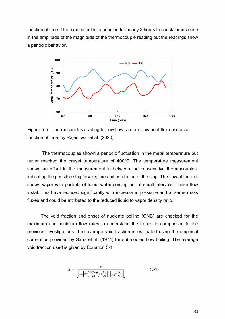
93

function of time. The experiment is conducted for nearly 3 hours to check for increase

in the amplitude of the magnitude of the thermocouple reading but the readings show

a periodic behavior.

Figure 5-5 : Thermocouples reading for low flow rate and low heat flux case as a

function of time; by Rajeshwar et al. (2020).

The thermocouples shown a periodic fluctuation in the metal temperature but

never reached the preset temperature of 400oC. The temperature measurement

shown an offset in the measurement in between the consecutive thermocouples,

indicating the possible slug flow regime and oscillation of the slug. The flow at the exit

shows vapor with pockets of liquid water coming out at small intervals. These flow

instabilities have reduced significantly with increase in pressure and at same mass

fluxes and could be attributed to the reduced liquid to vapor density ratio.

The void fraction and onset of nucleate boiling (ONB) are checked for the

maximum and minimum flow rates to understand the trends in comparison to the

previous investigations. The average void fraction is estimated using the empirical

correlation provided by Saha et al. (1974) for sub-cooled flow boiling. The average

void fraction used is given by Equation 5-1.

휀 = [𝑥

[𝐶𝑜[𝑥∗(𝜌𝑙−𝜌𝑔

𝜌𝑙) +

𝜌𝑔

𝜌𝑙]+[𝜌𝑔∗

𝑣𝑔𝑗

𝐺]]

] (5-1)

94

The average void fraction for the current investigations is estimated at the exit

by measuring the exit temperature of the fluid, flow rate, heat input to the system, inlet

pressure and other parameters and excluding the pressure drop. A distribution

parameter (Co) of 0.85 proposed by Ishii (2006) for vertically downward two-phase

flows is used for all the calculations. While correct estimation of Co and void fraction

plays an important role in general in two-phase flows, the results for basic checks

described are based on the information available in open literature and should be

treated only as qualitative trends. The void fraction is not determined explicitly from

the current experimental investigations.

Figure 5-6 shows the estimated average void fraction as a function of pressure

and for maximum throughput (~3000 kg/m2s) and minimum throughput (~58 kg/m2s)

cases. The basis for the maximum throughput and minimum throughput is defined in

the next section in terms of the flow rate. The results are shown for maximum and

minimum inlet fluid temperatures of 35oC and 70oC. The results are shown for 3.5 kW

heat input condition.

Figure 5-6 : Average void fraction estimate for low mass flux (58 kg/m2s) and high

mass flux (3000 kg/m2s) and inlet fluid temperatures of 35oC and 70oC with 3.5 kW

heat input by Rajeshwar et al. (2020).

From the Figure 5-6, the average void fraction increases marginally with

increase in the inlet fluid temperature for the low mass flux case (58 kg/m2s). At high

95

mass fluxes of 3000 kg/m2s, the inlet water temperature has negligible effect on the

average void fraction. The average void fraction estimated for low mass flux and at

atmospheric condition is 100% at the exit. The experiments have shown complete

vapor at the exit, validating the above trends, especially at atmospheric pressure. The

inlet fluid temperature has minimum effect at low mass flow rates and agrees well with

the observations from previous investigators (Mishima et al. (1984, 1985, 1987), and

Sudo et al. (1985, 1989). Previous investigators observed complete vapor at exit for

the low flow cases and for various inlet fluid temperatures. The void fraction is also

estimated using correlation given by Rouhani et al. (1970). The void fraction estimates

between both the models are comparable.

The onset of nucleate boiling calculations is performed for the current

investigations based on the empirical correlation provided by Bergles and Rohsenow

and as described in Mostafa Ghiaasiaan (2017). Equation 5-2 provides the empirical

correlation used for the estimate of onset of nucleate boiling. This calculation provides

a qualitative idea of the location where the bubble initiates and how much more space

is available in the test section for the CHF to occur.

(𝑇𝑤 − 𝑇𝑠𝑎𝑡)𝑂𝑁𝐵 = 0.556 [𝑞𝑤

"

1082𝑃1.156]𝑛

(5-2)

Where

𝑛 = 0.463𝑃0.0234

Figure 5-7 shows the ONB location for high mass flux (3000 kg/m2s) and low

mass flux (58 kg/m2s), at various pressures and for inlet fluid temperature of 35oC and

70oC. From Figure 5-7, the impact of the inlet fluid temperature is found to be negligible

at high mass fluxes. The CHF is observed mostly at the exit or in the last quarter of

the test section for high mass flux cases. However, at low mass fluxes, the onset of

nucleate boiling occurred much earlier compared to the high heat flux case. Further,

the case with high inlet fluid temperature shown much earlier ONB as compared to the

case with low inlet fluid temperature. The basic trends are compared from the current

investigations and found to be in good agreement with the trends reported by previous

investigations and as explained in the Chapter 2 of this thesis.

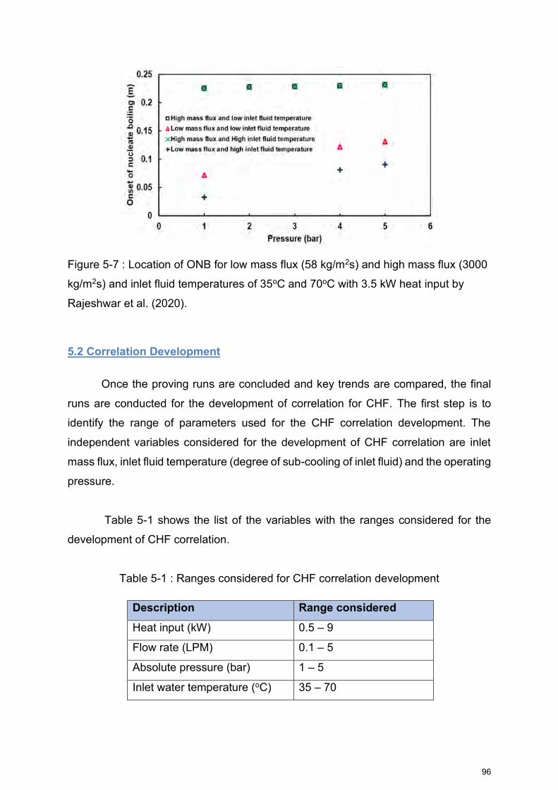
96

Figure 5-7 : Location of ONB for low mass flux (58 kg/m2s) and high mass flux (3000

kg/m2s) and inlet fluid temperatures of 35oC and 70oC with 3.5 kW heat input by

Rajeshwar et al. (2020).

5.2 Correlation Development

Once the proving runs are concluded and key trends are compared, the final

runs are conducted for the development of correlation for CHF. The first step is to

identify the range of parameters used for the CHF correlation development. The

independent variables considered for the development of CHF correlation are inlet

mass flux, inlet fluid temperature (degree of sub-cooling of inlet fluid) and the operating

pressure.

Table 5-1 shows the list of the variables with the ranges considered for the

development of CHF correlation.

Table 5-1 : Ranges considered for CHF correlation development

Description Range considered Heat input (kW) 0.5 – 9

Flow rate (LPM) 0.1 – 5

Absolute pressure (bar) 1 – 5

Inlet water temperature (oC) 35 – 70

97

There is no restriction heat input up to the maximum rating capacity of the

heaters. However, the resistances of the individual heaters are different and the heater

cannot be operated at its full rating capacity. This prompted the heat input to be

restricted to 9 kW. The flow rate and pressure dependency determined the range of

parameters considered for the current investigations. The pressure of 5 bar is fixed

based on the safety requirements and the strength calculations performed with the

test section pipe at elevated temperatures (per ASME B31.3) and including the

corrosion allowance. The same is explained in Chapter 4. The maximum flow rate

achieved at 5 bar pressure is 5 LPM and is fixed accordingly for the current

investigations. The heat losses from the Reservoir to the surroundings and the

external heater limitations restricted the maximum inlet sub-cooling temperature to

70oC. Further, to safeguard the pump from getting exposed to high temperature fluid,

the inlet fluid temperature is restricted to 70oC although the pump could be operated

till the temperatures of 90oC. The lower end of the temperature is fixed as average

room temperature on a hot day.

Once the variables are identified and the ranges are fixed, the next step is to

conduct the experiments to determine the CHF. Most of the previous investigators

increased the heat input in increments for given set of conditions till the CHF is

achieved. As the experiments are conducted at atmospheric pressure mostly, this

approach is reasonably quick as one of the variables of pressure is removed from the

calculations. However, it is not the case with current investigations and prompted to

look for an efficient way of conducting the experiments.

The present CHF investigations are carried out using a Design of Experiments

(DOE) approach to significantly reduce the number of experiments while capturing the

entire space based on the range of the parameters considered. Central Composite

Design (CCD) with face centered model is selected to develop the DOE matrix. CCD

model depends on the response surface. The main feature of the response surface

experiment is that it allows to include the quadratic effects. The response surface

experiment expands the form of the two-level empirical model by adding higher terms

including quadratic or cubic terms. The curvature in the CCD is achieved by

augmenting the star points to the fractional factorial matrix with center points. In

simpler terms, the CCD matrix in addition to factorial design of factors also considers

98

both center and axial points to capture the entire curvature. The Face-centered central

composite model has the star points on the square. The two-level factorial designs

quickly become too large as the number of factors increases, thus making the

fractional factorial design more advantageous (Mark et al. (1999) and Dodson et al.

(2014). In the current CCD matrix, 30 runs are considered with 3-star center points

and 3 cube center points. The DOE matrix is generated with Minitab (Mintab LLC,

USA) and Matlab version 2017 (Mathworks INC. USA) software for consistency

purposes.

A total of 30 runs are conducted based on the DOE generated using CCD

method and with the variables listed in Table 5-1. The experiments shown CHF risk

for almost all the cases except the cases with very low heat flux of 0.5 kW. This would

not help to achieve a proper CHF correlation as the bounds are not properly captured

as almost all the points shown the CHF risk. This prompted to relook into the range of

the heat input to capture the design space more effectively and to have optimal CHF

correlation estimation. Experiments are conducted for high mass flux (high flow rate

of 5 LPM) case with 35oC inlet temperature and at 5 bar pressure. The heat input is

increased in increments starting from 2 kW. The CHF is observed at a heat input of

3.5 kW and hence the 3.5 kW is set as the upper limit for the heat input range.

Table 5-2 provides the new set of ranges considered for the variables listed in

Table 5-1. DOE matrix is generated again with the new set of conditions and with the

same settings as used for the first DOE matrix. Table 5-3 shows the new DOE matrix.

Table 5-2 : Ranges considered for CHF correlation development

Description Range considered Heat input (kW) 0.5 – 3.5

Flow rate (LPM) 0.1 – 5

Absolute pressure (bar) 1 – 5

Inlet water temperature (oC) 35 – 70

99

Table 5-3 : Final DOE matrix for CHF correlation development

S. No. Pressure (bar) Inlet temperature (oC)

Flow rate (LPM)

Heat input (kW)

1 5 70 5 3.5

2 5 70 0.1 0.5

3 1 70 5 0.5

4 1 35 5 0.5

5 5 35 5 0.5

6 3 52.5 2.55 2

7 5 70 5 0.5

8 1 70 5 3.5

9 3 52.5 2.55 2

10 5 35 0.1 0.5

11 1 35 5 3.5

12 1 70 0.1 3.5

13 1 70 0.1 0.5

14 1 35 0.1 0.5

15 5 70 0.1 3.5

16 3 52.5 2.55 2

17 5 35 5 3.5

18 5 35 0.1 35

19 3 52.5 2.55 2

20 1 35 0.1 3.5

21 3 52.5 5 2

22 1 52.5 2.55 2

23 3 52.5 2.55 3.5

24 3 52.5 2.55 2

25 3 52.5 0.1 2

26 5 52.5 2.55 2

27 3 70 2.55 2

28 3 35 2.55 2

29 3 52.5 2.55 2

30 3 52.5 2.55 0.5

100

The above DOE matrix is developed based on ‘face centered CCD model’ and

has 6 center points, 3-star center points, 3 cube center points and 3 blocks to capture

the entire surface. A few of the points are repeated at discrete locations (not

continuous, order is important). This will ensure the repeatability and consistency of

the predictions.

Once the experiments are conducted for the DOE matrix and the runs are

completed, the bounds for the current experimental framework are established. A total

of additional 120 runs are considered to include the intermediate points within these

bounds. These cases are not listed in the Table 5-3. For the 120 additional points

considered, a few of the runs are eliminated based on visual elimination, a few of them

by a simple energy balance or the hand calculation, while rest of them by conducting

the experiments. The hand calculation procedure is defined in the Appendix D. Once

the results are obtained for all the cases, the points with CHF are taken and the CHF

correlation is developed using a non-linear regression analysis as described in Sarma

et al. (2006). A total of 102 points shown CHF risk and hence used for the correlation

development. The flow and the heat rate are translated to mass flux and heat flux. A

CHF correlation that is empirical in nature and makes no assumption about the

mechanisms involved in the CHF is developed. This correlation solely attempts a

functional relationship between the CHF and the independent variables (John et al.

(2001)). The CHF correlation developed based on these experiments is given by

Equation 5-3. The output file snapshot for the correlation is shown in the Appendix F.

𝒒𝑪𝑯𝑭,𝑫𝒓𝒆𝒇= 𝟗𝟑 ∗ 𝑷𝟎.𝟎𝟔𝟐𝟗 ∗ 𝑻𝒊𝒏

−𝟎.𝟎𝟑𝟖𝟔𝟕 ∗ 𝑮𝟎.𝟎𝟕𝟗𝟖𝟐 (5-3)

The above correlation holds good for the pressure in the range of 1 bar(a) to 5

bar (a), inlet fluid temperature up to 70oC, mass flux up to 3000 kg/m2s, and for circular

tubes of inner diameter of 6 mm, thickness of 1 mm, and with a length of 960 mm. The

diametric correction for the above CHF correlation is recommended based on the

Equation 5-4 provided by Ghiaasian (2017).

101

𝑞𝐶𝐻𝐹,𝐷 = 𝑞𝐶𝐻𝐹,𝐷𝑟𝑒𝑓∗ (

𝐷𝑟𝑒𝑓

𝐷)0.5

(5-4)

Equation 5-4 holds good for tube diameters up to 25 mm. The above CHF

correlation is developed based on the tube inner diameter and appropriate area

correction factor has to be used to determine the heat flux to be applied on outer

surface.

The present correlation agrees well with the experimental data with an average

deviation of 13.87% and standard deviation of 18.71%. The mean deviation is

comparable with some of the previous investigations listed by Chang et al. (1991).

Table 5-4 shows the comparison of average (mean) deviation and standard deviation

as listed by Chang et al. (1991) and for downward flows (upward/ downward flows).

Consistency runs are performed by picking some of the cases and conducting the

experiments again and check for the results. The consistency runs show that the

observations between both the experiments are almost identical with a maximum

deviation of ±2% observed, indicating the possible consistency of the results and the

experimental procedure itself on the whole.

Table 5-4 : Average and standard deviation by Chang et al. (1991) and comparison

with current data

Reference No. of data points

Mean error (%)

Std deviation (%)

Notes

KAIST (TS-1) 105 +6 14 P = 110 kPa, D =

0.006 m, L/d = 120

KAIST (TS-2) 40 +13.9 25.6 P = 110 kPa, D =

0.0088 m, L/d = 82

Mishima 84 -7.5 12.5 P = 101 kPa, D =

0.006 m, L/d = 57

Current

investigations

102 +13.87 18.71 P up to 5 bar, D =

0.006 m, L/d = 160

Once the correlation is developed, a few basic checks are performed to

compare the experimental data with the correlation prediction for various inputs within

102

the range considered. Figure 5-8 shows the comparison of the scatter of the CHF data

around the mean line as a function of non-dimensional mass flux. The non-

dimensional mass flux, represented by x-axis, is defined as the mass flux divided by

the maximum mass flux. The y-axis is the ratio of CHF estimated from correlation to

the CHF from the experiments.

Figure 5-8 : Comparison of calculated CHF value with correlation in comparison to

experimental data as a function of non-dimensional mass flux and for all the

pressure cases by Rajeshwar et al. (2020)

Figure 5-8 clearly indicates that most of the data points are within the ±30%

line. The current investigations show that the estimated values are more scattered at

low mass fluxes as compared to the high mass fluxes, indicating that the correlation

predicted value to be different to the experimental value. This is in line with some of

the previous investigations at low mass fluxes and low pressures. This could be

attributed to the dominance of two-phase flow instabilities at the low flow rates. At high

mass fluxes, more data is distributed closer to the mean line indicating that the

correlation predicted value and the experimental values are almost the same. The

results are shown for all the pressure cases, and for all the inlet fluid temperatures.

Figure 5-9 shows the comparison of the correlation value to the experimental

value at low mass flux of 58.6 kg/m2s, intermediate mass flux of 1400 kg/m2s and high

mass flux of 3000 kg/m2s, for water inlet temperature of 53oC, and at all pressures.

Trends from Figure 5-9 clearly show that the difference in estimated value from the

103

correlation and the experimental value increases with the decrease in pressure and at

low flow rate. The same trend is not observed at average and high mass fluxes,

indicating the possible complex flow mechanism associated with low mass flow rate

at low pressures as described by several previous investigators.

Figure 5-9 : Comparison of calculated CHF value to the experimental value at low,

intermediate and high mass flux, inlet temperature of 53oC and at all pressures; by

Rajeshwar et al. (2020).

A few qualitative trends are also checked with the developed correlation to

ensure that the trends are consistent with the current and the previous experimental

data. Figure 5-10 shows the influence of the mass flux on CHF at various pressures

and for fixed inlet fluid temperature. As it is evident from Figure 5-10, the CHF

magnitude increases with increase in pressure. The increase is found to be 10-12%

for 5 bar pressure when compared with 1 bar pressure. The chart shown is for different

Lcritical/D and critical quality.

A CHF correlation is developed as a function of mass flux, inlet pressure and

inlet fluid temperature up to pressures of 5 bar. The developed correlation agrees well

with the experimental data at high mass fluxes, high pressures but deviates at low

pressures and low mass fluxes. The trends observed from the current investigations

are in line with most of the previous investigations. The standard deviation and the

mean deviation from the developed correlation are comparable or better than reported

standard and mean deviations based on previous investigations.

104

Figure 5-10 : Qualitative trends from current investigations – influence of mass flux

on CHF at various pressures; by Rajeshwar et al. (2020).

One of the most important things that needs the due attention is the confidence

level on the current predictions. Uncertainty analysis is mandatory to study to

determine the confidence levels. Next chapter discusses about the uncertainty

analysis carried out as part of the current investigations.

105

Chapter 6 Uncertainty Analysis

The CHF correlation developed from current experimental investigations shows

a reasonable mean and standard deviation as explained in the previous chapter. This

indicates how good the estimated correlation data fits in comparison with the actual

experimental data. However, one of the biggest questions that arise with the

experiments is the reliability of the data itself. The reliability of the data refers to the

ability to predict the true and accurate result for a given set of conditions by eliminating

all the errors that could arise due to instrumentation, improper measurement, and

errors due to unknown sources commonly termed as random errors. The difference in

the true value and the measured value is the error in the measurement. It is neither

possible to measure the true value with cent percent accuracy nor it is possible to

identify all the errors. As a result, the experimental results always come with certain

level of uncertainty. The term uncertainty refers to the interval around the measured

value within which the true value is expected to exist. It is important to determine and

report this uncertainty for any experimental investigations and thereby build the

confidence levels on the experimental results. Without quoting the uncertainty

intervals, it is difficult to accept the experimental intervals as quoted by Moffat (1988).

Kline et al. (1953) provided good insights of describing the uncertainties in

single sample experiments. The methodology described by Kline et al. is still being

used to determine the uncertainty intervals in which the true value is believed to lie. It

is easy to build the confidence level in multiple-sample experiments as there is a

provision to repeat the experiments with same set of conditions and thereby eliminate

possible errors, if any. However, it is not true in most of the situations. The cost

implications, the complexity and the safety concerns associated with conducting these

experiments and other related factors would make it challenging to repeat the

experiments. Experiments in which the uncertainties are not determined by the

repetition are termed as single sample experiments. As the experiments are

conducted without repetition (except for a few cases for consistency checks), it falls

into the category of the single sample experiments. The procedure described by Kline

is applied for the current investigations to conduct the uncertainty analysis. The next

section discusses briefly about the uncertainty analysis followed by the uncertainty

analysis procedure carried out as part of the current investigations.

106

The procedure as mentioned in Moffat is explained below for reference. The

same procedure is used for current investigations to determine the uncertainty interval

for the experimental results. If R is the result and is a function of ‘n’ independent

variables x1, x2, x3, …………, xn, then R is measured as R = R (x1, x2, x3, ----, xn). The

objective is to express the uncertainty in the calculated result by estimating the

uncertainties in the measurements of all the individual variables. The uncertainty due

to error from a single measurement and its impact on the calculated result is given by

Equation 6-1.

𝛿𝑅𝑥𝑖=

𝜕𝑅

𝜕𝑥𝑖𝛿𝑥𝑖 (6-1)

Similarly, the uncertainty due to error from all the measurements and its impact on the

calculated result is given by Equation 6-2.

𝛿𝑅 = {∑ (𝜕𝑅

𝜕𝑥𝑖𝛿𝑥𝑖)

2𝑛𝑖=1 }

1/2

(6-2)

Equation 6-2 constitutes the fundamental equation of the uncertainty analysis.

Each term in the Equation 6-2 represents the contribution made by the individual

variable to the overall uncertainty in the final result 𝛿𝑅. It should be noted that the

above equation applies as long as the following conditions are applied (Moffat, 1998).

1. Each measurement is independent.

2. If repeated observations are made for each measurement, they would display

Gaussian distribution

3. The uncertainty in each measurement is expressed at the same odds initially.

In many situations, the uncertainty estimate could be based on fraction of

reading rather than based on engineering units. In such situations, it is possible to

calculate the relative uncertainty directly, especially whenever the equation describing

the result is in a pure product form as given by Equation 6-3.

𝑅 = 𝑥1𝑎𝑥2

𝑏𝑥3𝑐𝑥4

𝑑 …………𝑥𝑀𝑚 (6-3)

107

Equation 6-4 gives the relative uncertainty in direct form and is natural and

convenient approach where the uncertainties of the component measurements are

described in percent of reading.

𝛿𝑅

𝑅= {(𝑎

𝛿𝑥1

𝑥1)2

+ (𝑏𝛿𝑥2

𝑥2)2

+ ⋯+ (𝑚𝛿𝑥𝑚

𝑥𝑚)2

}1/2

(6-4)

In the current investigations, a single sample experiments uncertainty method

is used to determine the uncertainty in the output predicted by the CHF correlation

developed as part of these predictions. The measurement errors arising due to

instruments and the heat input are considered for the uncertainty analysis. Random

errors like flow variation due to pump fluctuation etc. are ignored from the current

investigations. Table 6-1 shows the list of instruments used and the errors associated

with each of its instruments. Wherever, the calibration error is not found, the least

count of the instrument is considered as the possible error.

Table 6-1 : Specifications of the instruments used in current investigations

Parameter Instrument Range/ Resolution

Accuracy

Inlet fluid temperature K-type probe 300oC/ 0.1oC ±1oC

Metal Temperature Chromel-Alumel

Thermocouples

1260oC/ 0.1oC ±1oC

Fluid Temperature Long stem thermometer

probes

300oC/ 1oC ±2oC

Pressure Pressure Gauge 0-7 bar/ 0.1 bar ±0.2 bar

Flow Rate Rotameter 0-7 LPM/ 0.1

LPM

±1.5%

Power Input/ Voltage Variac 240 V/ 2 V ±2 V

For the current investigations, the flow is measured with both the flow meter

(rotameter) and the manual measurement as explained in previous chapters. For the

uncertainty analysis, the flow measurement is considered based on the manual

measurement as it became difficult to determine the uncertainty with the flow meter

108

(rotameter), especially at low flow rates due to its resolution. Even finding a continuous

constant reading accurately at high flow rates using rotameter was a challenge due to

fluctuation in the float. Multiple readings are taken from manual measurement and an

average time and the average volume was taken while performing the uncertainty

analysis.

The output CHF for the current investigations is dependent on the mass flux,

pressure, inlet subcooling and the heat input. The following section describes the

uncertainty analysis performed on the input variables and its impact on the output

CHF. Equation 6-5 shows the general form considered for the current investigations.

QCHF = f {P, Tin, G [=f (flow rate, d)]} (6-5)

The heat input also has the uncertainty due to fluctuation in voltage and is

considered for the uncertainty analysis. As the correlation developed is in pure product

form, the direct form as given in Equation 6-4 is used for the current uncertainty

analysis. The uncertainty estimates for the individual independent parameters are

discussed below.

Uncertainty in Pressure:

The possible error in pressure measurement arises from two sources:

1. Calibration error of the instrument

2. Pressure fluctuation observed during the operation, especially at high pressure.

Pressure variation due to instrument: ±0.1 bar

Pressure variation due to fluctuation: 0.2 bar

Total variation in pressure: 0.3 bar

The maximum pressure at which this variation could be observed is at 5 bar.

Hence the total uncertainty is estimated as the ratio of total variation in pressure (0.3

bar) to the maximum pressure (5 bar). The uncertainty in measurement is ~6%.

Although, the maximum uncertainty would have achieved with 1 bar pressure (0.3/1 =

30%), it is theoretically difficult to achieve that level of uncertainty at low pressures.

109

Uncertainty in Temperature:

The possible error in temperature measurement arises from two sources:

1. Calibration error

2. Temperature difference in the reservoir W1 (from where the water is supplied

during the experiment) due to the possible stratification observed during the

operation.

Temperature variation due to instrument: ±1oC

Temperature variation in the reservoir: ±2oC

Total variation in temperature: 3oC

Minimum temperature at which the maximum uncertainty could be observed is

at 35oC. Hence the total uncertainty is estimated as the ratio of total variation in

temperature (3oC) to the minimum temperature (35oC). The uncertainty in

measurement is ~8.6%.

Uncertainty in Mass Flux:

The uncertainty in the mass flux depends up on uncertainty of two independent factors:

1. Volumetric flow rate measurement (manual measurement as rotameter

measurement is not considered)

2. Variation in the diameter of the test pipe

The uncertainty in the volumetric flow rate measurement itself depends on two factors:

1. Volume measurement in the measuring jar.

2. Time measurement based on stop clock.

Least count of the measuring jar: 10 mL

Uncertainty in the measurement: ±5 mL (Least count/2)

Total volume of the measuring jar: 500 ml

The uncertainty in the measuring jar measurement is the ratio of uncertainty in the

measurement (5 mL) to the total volume of the measuring jar (500 mL), which

translates to 1%.

110

The time uncertainty depends on the least count of the stop watch.

Least count of the time measurement: 1 sec

Uncertainty in the measurement: ±0.5 sec

Time to fill 500 ml: 6 sec

The total uncertainty in the measurement of the time is the ratio of uncertainty in the

measurement (0.5 sec) to the minimum taken to fill the 500 mL (6 sec), which

translates to ~8.3%.

The total uncertainty in the flow measurement is the root of the sum of the square of

the time uncertainty (8.3%) and the square of the flow measurement (1%). This gives

the total flow uncertainty as ~8.4%.

The uncertainty in area calculation depends on the diameter of the pipe.

Inner diameter of the pipe: 6 mm

Variation in the measurement of diameter: 0.5 mm (based on actual measurements

and the inputs provided in open literature)

Actual variation: 0.25 mm (Least count/2)

The total uncertainty in the area measurement is the ratio of actual variation (0.25 mm)

to the inner diameter of the pipe (6 mm) whole multiplied by 2. Since the area has

square term, the derivative would be twice the diameter. This gives a total uncertainty

in the area to be ~8.3%.

The mass flux variation is given by the root of the sum of the square of the

uncertainty in the volumetric flow rate (8.4%) and the uncertainty in area measurement

(8.3 %). This gives the overall mass flux uncertainty as 11.8%. It should be noted that

the density variations are neglected during the calculation of uncertainty in mass flux.

Uncertainty in Heat Input:

One of the major sources of error is the supplied heat to the test section. The

heat input depends on two independent variables (ignoring all the other variables

contribution, which are considered to be small)

1. Variation in power input due to change in voltage.

2. Variation in outer surface area on which the entire heat is imposed.

111

Variation in the voltage: ±2 V (measurements)

Minimum voltage to get maximum uncertainty: 48 V (Based on the lowest heat input

for the test section)

The total uncertainty in the voltage or the power input is given by the ratio of variation

in voltage (2 V) and the minimum voltage to get maximum uncertainty (48 V). This

translates to an uncertainty of ~4.2% ignoring the resistance variations.

The surface area variation in the tube is due to two independent variables.

Variation in the diameter of test piece.

Variation in the length of the test piece.

Outer diameter of the pipe: 8 mm

Variation in the measurement of diameter: 0.5 mm (based on actual measurements

and the inputs provided in open literature)

Actual variation: 0.25 mm

Length of the pipe: 960 mm

Actual length variation: 30 mm (assumed the diameter and the length variation are the

same as there is no direct measurement)

The uncertainty in the diameter is the ratio of the actual diameter variation (0.25 mm)

to the outer diameter of the pipe (8 mm), which translates to ~3.1%. The uncertainty

in the length is the ratio of the actual length variation (30 mm) to the total length of the

tube (960 mm), which translates to ~3.1%. The total uncertainty in the surface area is

the root of the square of the sum of the diameter uncertainty (3.1 %) and the length

uncertainty (3.1%). This gives a total surface area uncertainty of ~4.4%.

The total uncertainty in the heat flux is the sum of the uncertainty due to surface area

and the heat flux, which results in ~8.6%.

Total Uncertainty in Output:

The developed CHF correlation from the current experimental investigation as

described in the previous chapter is given below.

112

𝑞𝐶𝐻𝐹,𝐷𝑟𝑒𝑓= 93 ∗ 𝑃0.0629 ∗ 𝑇𝑖𝑛

−0.03867 ∗ 𝐺0.07982

As explained earlier, the above equation is in pure product form and the Equation 6-4

is used to determine the uncertainty. The total uncertainty in the output is due to

1. Uncertainty in the independent variables of pressure, inlet fluid temperature and

the mass flux.

2. Uncertainty in the heat input due to variation in surface area and the voltage.

The uncertainty due to independent variables of pressure, inlet fluid temperature and

mass flux is defined as the root of the sum of the square of the pressure uncertainty

times 0.0629, square of the temperature uncertainty times -0.03867 and square of

mass flux uncertainty times 0.07982. This gives the total uncertainty due to

independent variables as ~0.84%.

The uncertainty in the heat input due to variation in surface area and the voltage

variation is ~8.6%.

The total uncertainty for the current investigations is the sum of the uncertainty in the

heat input (8.6%) and the uncertainty due to measurement in independent variables

(0.84%). This gives a total uncertainty of 9.4%. This indicates that the results from the

current experimental investigations/ correlation have a confidence level of ~91% and

is a major conclusion from the current investigations. Table 6-2 shows the uncertainty

numbers quoted by authors based on their investigations carried out (Chang et al.

(1991) and Ruan et al. (1993)). The previous experiments reported the confidence

levels of 95%.

Table 6-2 : Specifications of the instruments used in current investigations Description Uncertainty Chang et al. (1991) Outlet pressure (kPa) ± 1

Inlet sub-cooling (kJ/kg) ± 5

Mass flux ± 5%

113

Total heat flux ± 4%

Ruan et al. (1993) Pressure – electric pressure transducer (kPa) ± 5

Flow rate - turbine flow meter ± 1.5%

Inlet temperature – resistance thermometer (K) ± 1

Wall temperature – chromel-alumel thermocouple (K) ± 1

Voltage – voltage divider ± 1%

Current – shunt ± 0.5%

Overall CHF – average heat flux calculated by dividing

heating power by heating area

± 4%

The results and observations from the current experimental investigations, the

development of CHF correlation and the uncertainty estimates based on the current

experiments concludes the main objective of the current research. In the next chapter,

the numerical analysis carried out as part of these investigations is discussed along

with the comparison of CHF correlation developed from the numerical analysis with

the CHF correlation developed based on current experiments.

114

Chapter 7 Numerical Modeling and Results

The CHF correlation developed based on the experimental investigations are

discussed in previous chapters. The uncertainty analysis carried out to build the

confidence levels on the predictions of the experimental results and thereby on the

estimations from the CHF correlation are also established. While conducting the

experimental investigations are mandatory to meet the final objective for any design

concept, they are expensive and are time consuming. If the number of experimental

test runs required are plenty, this could further delay to meet the end objective. This

prompted for looking for alternatives for the experimentation during the initial screening

of the design concepts. Numerical simulations are one of the effective solutions. With

rapid advancements in computational resources and hardware, numerical tools gained

popularity over conventional methods. The validated numerical models not only

reduced the cost of conducting experiments but also reduced the timelines for the

introduction of the design into the market. The validated numerical models also gave

good insights of the flow and the temperature patterns inside the component for

aerothermal problems and the stress/ strain information for mechanical problems even

before the prototype is developed. This helped in optimizing the design well in advance

before arriving at the final prototype design to be built for the final testing. The inherent

advantages associated with the numerical modelling prompted to investigate the

available two-phase models commercially available in markets and validate the same

with the experiments carried out as part of these investigations for vertically downward

two-phase flows. This section discusses the numerical modelling carried out on two-

phase flows in vertically downward tubes. The first few pages discuss about the

conservation equations and the closure equations followed by the investigations

carried out as part of the current studies.

7.1 Governing and Closure Equations

For current investigations, commercially available numerical tool Fluent by

ANSYS Inc. USA, is used. As the investigations are held over a period, different

revisions of the tool are used. The convergence strategies, the modelling principles as

described in the user’s manual [ANSYS documentation] is used for the current

115

investigations. An Eulerian multiphase boiling model is used for all the simulations.

The RPI (Rensselaer Polytechnic Institute) boiling model, non-equilibrium boiling

model and the CHF model available in Fluent are used in the investigations. The Fluent

solves a set of governing and closure equations. Huiying et al. (2011) explained the

equations used to simulate boiling and critical heat flux models available in Fluent. A

brief description of the governing and closure equations are provided below for ease

of discussion. Equations 7-1, 7-2, and 7-3 specifies the conservation of mass,

momentum, and energy for any phase.

∂(αqρq)

∂t+ ∇ ∙ (αqρqV q) = ∑ (mrq − mqr)

nr=1 + Sq (7-1)

∂(αqρqV q)

∂t+ ∇ ∙ (αqρqV qV q) = −αq∇p + ∇ ∙ (τq) + αqρqBf

+ ∑ (F rqD +F rq

TD + mrqV rq −n

r=1

mqrV qr) + F q+F qL+F q

vm (7-2)

∂(αqρqHq)

∂t+ ∇ ∙ (αqρq

V qHq) = τq: ∇. V q + αq∂p

∂t− ∇. q + SH,q + ∑ (qrq

+mrqHrq−mqrHqr)nr=1

(7-3)

The K-epsilon RNG (Renormalized group) turbulence model is used for all the

simulations. The generalized turbulence scalar equation is given by the Equation 7.4.

∂(αqρq∅q)

∂t+ ∇ ∙ (αqρqV q∅q) = ∇ ∙ (αqΓϕ,q∇∅q) + αqS∅,q (7-4)

In the RPI wall boiling model, the total heat flux from wall is divided into 3 components:

• Liquid phase convective heat flux: for convective heat flux to the liquid, given

by Equation 7-5

��𝐶 = ℎ𝐶(𝑇𝑤 − 𝑇𝑙)(1 − 𝐴𝑏) (7-5)

• Quenching heat flux: to quench the heated wall post departure of the bubble,

given by Equation 7-6.

116

��𝑄 = 𝐶𝑤𝑡2𝑘𝑙

√𝜋𝛾𝑙

𝑓𝑏𝑤⁄

(𝑇𝑤 − 𝑇𝑙𝑞)𝐴𝑏 (7-6)

• Evaporative heat flux: for evaporation of the liquid within the vicinity of the wall,

given by Equation 7-7.

��𝐸 =𝜋

6𝑑𝑏𝑤

3 𝑓𝑏𝑤𝑁𝑤𝜌𝑣𝐻𝑙𝑣 (7-7)

Equations 7-5 to 7-7 requires closure equations.

The first term Ab defined as area of influence and is given by Equation 7-8.

𝐴𝑏 = min (1, 𝜂𝜋

4𝑑𝑏𝑤

2 𝑁𝑤) (7-8)

Where the empirical coefficient 𝜂 can be estimated using correlation proposed by Del

Valle and Kenning and given by Equation 7-9.

𝜂 = 4.8 exp (−𝐽𝑎

80) (7-9)

Ja is the Jacob number given by equation 7-10.

𝐽𝑎 =𝜌𝑙𝐶𝑝𝑙Δ𝑇𝑠𝑢𝑏

𝜌𝑣𝐻𝑙𝑣 (7-10)

The frequency of bubble departure from the wall is proposed by Cole and is

controlled by the inertia growth. The Equation for the frequency of the bubble

departure is given by Equation 7-11.

𝑓𝑏𝑤 = √4𝑔(𝜌𝑙−𝜌𝑣)

3𝜌𝑙𝑑𝑏𝑤 (7-11)

The bubble departure diameter is proposed by various authors Tolubinski-

Kostanchuk, Unal, Kocamustafaogullari-Ishii (Huiying, 2011). For current

investigations, Tolubinski-Kostanchuk correlation is used and hence the same is

defined by Equation 7-12.

𝑑𝑏𝑤 = min {𝑑𝑏𝑤,𝑚𝑎𝑥, 𝐶𝑏𝑤𝑒𝑥𝑝 (−Δ𝑇𝑠𝑢𝑏

45)} (7-12)

117

dbw.max default value is 0.0014 and cbw default value is 0.0006.

The nucleation site density is given by Lemmert-Chawla and determined by Equation

7-13.

𝑁𝑤 = 𝐶(Δ𝑇𝑠𝑢𝑝)𝑚 (7-13)

Where the default values for C and m are 15545.54 and 1.805 respectively.

The other closure models used for the calculations are defined below. More

details could be read from the ANSYS documentation (ANSYS, Huiying et al. (2011)).

• Drag force: Ishii correlation

• Lift force: Moraga

• Wall lubrication: Antal et al.

• Turbulent dispersion: Lopez-de-bertodano

• Turbulent interaction: Troshko-Hassan

• Heat Transfer: Ranz Marshall

• Interfacial area: ia-symmetric

7.2 Validation of CFD Models – Void Fraction & CHF

The applicability of the numerical models is questionable unless it is validated

with the experimental data. In the current investigations, the first step is to validate the

void fraction and the CHF models with the experimental results published by previous

investigators. Most of the authors validated their CFD modelling for void fraction using

the experimental data published by Bartolomei et al. (1967). For the current

investigations, the numerical analysis procedure adopted by Sumanth et al. (2018) is

used. Sumanth et al. (2018) validated the CFD models with the experimental data by

Bartolomei et al. (1967) for void fraction and the experimental data by Hoyer (1998)

for CHF. The grid independence studies are conducted before conducting the final

simulations and the results shown not much variation (Sumanth et al (2018)). Figure

7-1 (a) shows the grid independence studies results. Figure 7-1 (b) shows the

validation of the void fraction from the numerical investigations by Sumanth et al.

118

(2018) with the experimental data by Bartolomei et al. (1967). As it is evident from

Figure 7-1 (b), the void fraction estimates from the numerical simulations for vertically

upward two-phase flows are in good agreement with the experimental data. The

validated models are extended for vertically downward two-phase flows with the same

settings. Figure 7-3 shows the void fraction profile for vertically downward two-phase

flow and vertically upward two-phase flow. As it is evident from Figure 7-3, the void

fraction profiles are almost comparable, indicating the applicability of the validated

vertically upward two-phase flow models to simulate vertically downward two-phase

flows. This is in line with some of the previous investigator’s observations that the flow

direction has no impact at high mass fluxes (Mishima et al. (1985, 1987) etc.).

Figure 7-1 (a): Grid indpenence studies results; (b): Void fraction comparison with

experimental data by Bartolomei et al. (1967) and current numerical simulation by

Sumanth et al. (2018) for vertically upward flow.

Once the models are validated for void fraction and extended for downward

flows, the second step is to check the applicability of the available models in Fluent for

CHF predictions. The validation is performed with the experimental work by Hoyer

(1998). These simulations are also carried at high pressure. The boundary conditions

and the other geometric details could be retrieved from the investigations carried by

Sumanth et al. (2018).

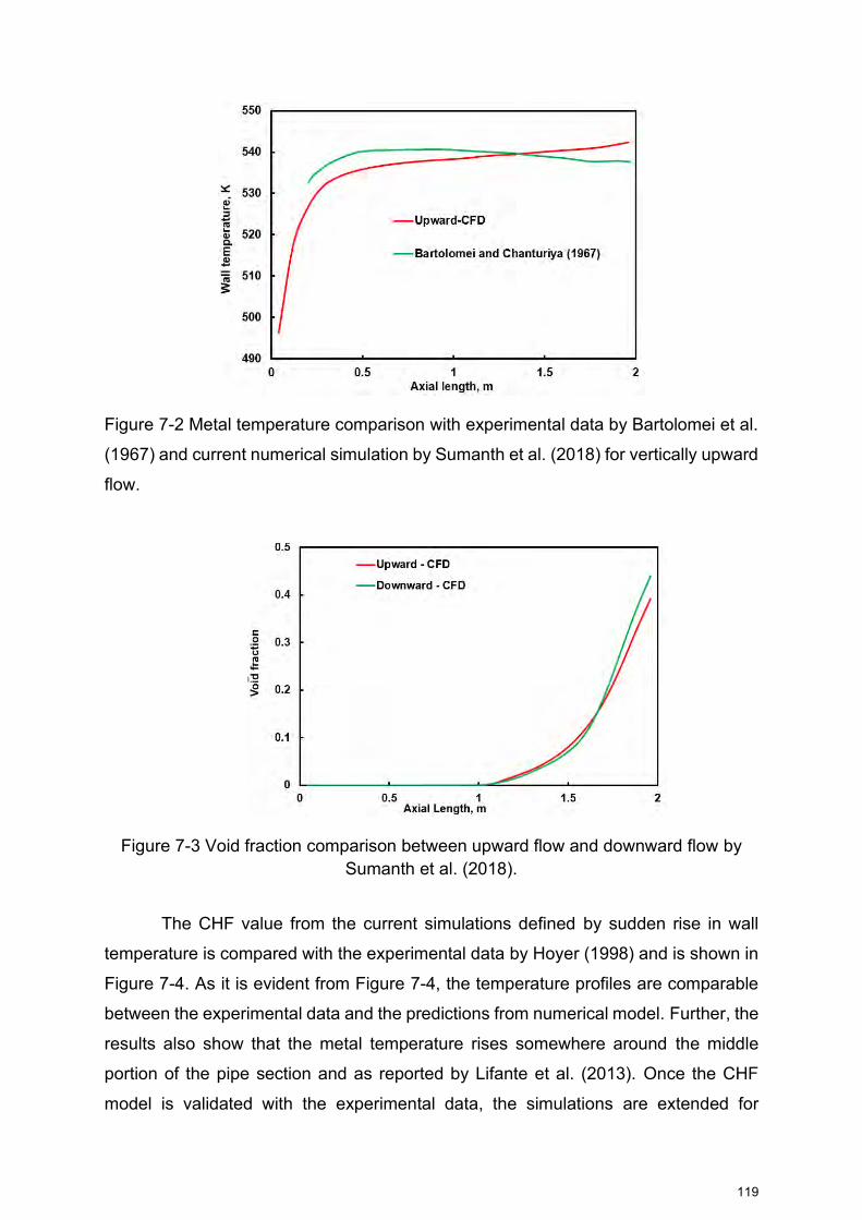
119

Figure 7-2 Metal temperature comparison with experimental data by Bartolomei et al.

(1967) and current numerical simulation by Sumanth et al. (2018) for vertically upward

flow.

Figure 7-3 Void fraction comparison between upward flow and downward flow by Sumanth et al. (2018).

The CHF value from the current simulations defined by sudden rise in wall

temperature is compared with the experimental data by Hoyer (1998) and is shown in

Figure 7-4. As it is evident from Figure 7-4, the temperature profiles are comparable

between the experimental data and the predictions from numerical model. Further, the

results also show that the metal temperature rises somewhere around the middle

portion of the pipe section and as reported by Lifante et al. (2013). Once the CHF

model is validated with the experimental data, the simulations are extended for

120

downward flow with the same settings except swapping the inlet and the outlet. Gravity

direction is taken care during the simulations. The results for the metal temperature

for vertically downward flow and comparison with the upward flow is shown in the

same Figure 7-4. The temperature profile for upward and downward flows are almost

identical. This provided enough confidence on the models to be used to simulate

vertically downward two-phase flows.

Figure 7-4 CFD predictions for CHF (metal temperature) for upward flow and

comparison with the experimental data by Hoyer (1998) and extending to downward

flow [Sumanth et al., 2018]

Once the CHF model is validated for vertically upward flow and the modeling

techniques are established to extend them for vertically downward flows, simulations

are performed at the experimental conditions carried out as part of these

investigations. However, a lot of challenges are encountered when simulations are

conducted at current experimental conditions, especially from convergence

perspective. As indicated in earlier chapters, literature search revealed hardly any

numerical simulations carried with the existing CHF models at low pressures and

hence convergence techniques are not fully established. Further, discussion with

experts from ANSYS revealed that the convergence strategy at low pressures is not

established and is by trial and error. This prompted to look into more details to

understand the pressures to which the solution could be converged with standard

settings. Rajeshwar et al. (2019) conducted numerical investigations by varying the

pressures from 7.01 MPa (70.1 bar) to 0.1 MPa (1 bar) and in combination of two set

121

of mass fluxes, two set of heat fluxes and two set of inlet sub-cooling temperatures.

The simulations are carried with same set of relaxation factors and for both vertically

upward and vertically downward two-phase flows. Figure 7-5 (a-d) shows the

convergence difficulties associated with the simulations. In the Figure 7-5, the y-axis

shows the line of convergence. Every point that falls below the horizontal line indicates

the convergence of the solution while the points above the horizontal line indicates

that the solution is not converged. Results are shown for both upward flow and

downward flow and with two different inlet sub-cooling temperatures of 10K and 40K.

The continuous lines are shown for the upflow while the dotted lines are shown for the

downflow. The lines with red color are shown for the 40K inlet sub-cooling while blue

color are shown for upflow with 10K inlet sub-cooling. Figure 7-5(a) refers to the low

mass flux (497 kg/m2s) and low heat flux (350 kW/m2), Figure 7-5(b) refers to low mass

flux (497 kg/m2s) and high heat flux (1500 kW/m2), Figure 7-5(c) refers to the high

mass flux (2000 kg/m2s) and low heat flux (350 kW/m2), and Figure 7-5(d) refers to

high mass flux (2000 kg/m2s) and high heat flux (1500 kW/m2).

Figure 7-5 Convergence with reference to pressure for various mass and heat fluxes

and with different inlet sub-cooling temperatures. (a) low mass flux and low heat flux

122

(b) low mass flux and high heat flux (c) high mass flux and low heat flux (d) high mass

flux and high heat flux [Rajeshwar et al., 2019].

As it is evident from the Figure 7-5 (a-d), most of the cases show better

convergence for pressures 1.5 MPa (15 bar) or above (Rajeshwar et al. (2019)). As

the current experiments are conducted below 0.5MPa (5 bar), the convergence

difficulties is found to be profound. It should be noted that the above results are with

fixed settings. The next section discusses about the solution strategies adopted to

converge the solution for the experimental conditions, develop a CHF correlation and

compare the same with the experimental conditions.

The CFD simulations are carried with a series of trials and errors. The main

focus is given on the pseudo-time scales, under relaxation factors, and other critical

parameters that could influence the solution. Figure 7-6 shows the computational

domain used for the current investigations. It is same as the experimental rig test

section pipe dimensions.

Figure 7-6 Computational domain for experimental test rig [Rajeshwar et al., 2020]

123

The following major assumptions are made for the CFD investigations.

1. 2d axi-symmetric

2. The gaps for the thermocouple locations in the experiments are ignored for

current simulations.

3. Metal (conjugate heat transfer) is not modeled.

4. Simulation is stopped where the metal temperature shows abrupt rise in

metal temperatures.

The preliminary simulations are carried to understand the strategy to be formulated

for convergence. The simulations are carried for high and low mass flux, high and low

heat flux and at atmospheric pressure conditions. Several trial and combinations are

investigated before finalizing the strategy. The following list of items are proven to give

optimal settings for the convergence for vertically downward two-phase flows at low

pressures and in Fluent simulation software.

1. Single precision solver is used instead of double precision solver. Some of the

cases shown convergence with double order precision while most of them

shown convergence with single order precision solver.

2. First order upwind scheme for volume fraction and second order upwind

scheme for all the other equations and pressure-velocity coupling with coupled

solver. Some of the cases shown difficulty in convergence with second order

upwind scheme and hence switched back to first order upwind scheme.

3. Pseudo-transient option and higher order relaxation terms switched on in

solution methods. :

4. The following under relaxation factors range are dominantly used for the

simulations.

a. Pressure : 0.15 - 0.3

b. Momentum: 0.4 - 0.5

c. Density: 0.5

124

d. Body forces: 0.5

e. Volume fraction: 0.05 - 0.1

f. Vaporization mass: 0.05 - 0.1

g. Turbulent kinetic energy: 0.1

h. Turbulent dissipation rate: 0.15

i. Turbulent viscosity: 0.1

j. Energy: 0.3 - 0.5

5. While most of the cases converged with above said settings, there are a few

cases that were simulated with very low urfs till the solution stabilized and then

slowly incremented to arrive at the solution.

6. The maximum turbulent viscosity ratio is set to 1e14 value instead of default

value.

7. The timescale factor used for majority of the calculations is 0.3 while for a few

cases, a value of 0.75 is used.

The above settings are optimal settings for the current solution and could vary for

case to case and cannot be taken as final values for all the cases. The y+ value is

taken care during the simulation as per one of the requirements for the mass transfer

in the boiling model. The grid elements used are hexahedral and the grid size is

~60000. The velocity and turbulent parameters are established for each and every

case based on cold flow before using the fully developed profiles as input conditions

for the boiling simulations. The fully developed flow profiles are taken from cold flow.

Verbosity is switched on to understand the divergence parameter for some of the

troubled cases. The properties are considered as a function of temperature for both

liquid and vapor phases and are taken from steam tables (Chemicalogic, 2003). The

details of the properties used for current simulations are provided in Appendix B. The

care is taken for defining the standard state enthalpy as this dictates the accuracy of

the solution.

125

7.3 Correlation Development using CFD

Once the parameters are defined, the CFD simulations are carried out for the DOE

matrix used for the experimental test rig described in Chapters 4 and 5. A few of the

intermediate points are also considered. The simulations are carried out till the abrupt

rise in metal temperature is observed for each of the cases. The details of the DOE

matrix is provided in the subsequent sections. The high level input conditions for the

current simulations are provided in Table 7-1.

Table 7-1 : High level boundary and input conditions for the current numerical simulations

Description Unit Range

Operating Pressure bar 1-5

Mass Flux kg/m2s 50-3000

Inlet Temperature of Fluid oC 35-70

Figure 7-7 shows the comparison of the critical heat flux values from current

numerical simulations and the experimental data/ correlation at different pressures,

low mass flux of 50 kg/m2s and inlet fluid temperature of 35oC.

Figure 7-7 Comparison of numerical models for CHF with the test data by Rajeshwar

et al., (2020) for low mass flux (50 kg/m2s); chart from Rajeshwar et al. (2020).

126

As it is evident from Figure 7.7, the results from current CFD matches well with the

experimental data at low mass flux of 50 kg/m2s. Figure 7-8 shows the maximum metal

temperature monitor point on the wall of the tube. The result is shown for the low flow

rate case of 50 kg/m2s and at atmospheric pressure, where CHF is observed. There

is an abrupt rise in temperature exceeding the safe limit 673K (400oC) as explained

earlier.

Figure 7-8 Monitor point for metal temperature for the CHF case with low mass flux

by Rajeshwar et al. (2020).

Figure 7-9 shows the volume fraction at the exit of the tube for the same low mass

flux case. As it is evident from Figure 7-9, the vapor volume fraction at exit is close to

80%, indicating significant amount of vapor phase present at the exit. The same trend

is observed from experimental investigations. The experimental investigations also

shown significant amount of vapor with a periodic flow of water droplets at the outlet.

Thus, the CFD predictions show comparable trends with the experimental data at low

flow rate case of 50 kg/m2s.

Figure 7-10 shows the comparison of the numerical results with the experimental

data at all pressures and for high mass flux case of 3000 kg/m2s and with inlet fluid

temperature of 35oC. As it is evident from Figure 7-10, the results deviate significantly

when compared with the experimental data. The variation observed is by an order of

magnitude. The simulations with the actual heat flux values did not show any CHF

risk. So, the heat flux is increased in increments till the CHF is observed for the high

mass flux case. All the intermediate flow rates also shown significant variation when

127

compared to the experimental data but the deviation is smaller than what is observed

for the high mass flux case of 3000 kg/m2s. The procedure adopted for high mass flux

is used for the intermediate mass fluxes as well. Further investigations are required to

understand the reasons for such behaviour of the numerical simuations and is beyond

the scope of the current investigations. However, current assessment indicates that

the existing models or the same CFD case setup would not be applicable for all the

mass flux cases, especially at such low pressures. Further, the role of the entry effects

should be investigated as the numerical simulations assume a fully developed flow

while the experiments shown entry effects dominance.

Figure 7-9 Monitor point for vapor volume fraction at outlet for the CHF case with low

mass flux by Rajeshwar et al. (2020).

Comparisons are also made from the current numerical simulations with the

experimental data published by Mishima et al. [1985] with length correction. The

experiments by Mishima et al. are conducted with inlet throttling and/or inlet plenum.

Figure 7-11 shows the comparison of the numerical results with the experimental data

published by Mishima et al. As it is evident from Figure 7-11, the numerical results

from current simulations under predict slightly when compared with the experimental

data published by Mishima et al. CFD model predictions are close to the experimental

results at higher mass fluxes where the inlet plenum/ inlet throttling effects are

included. These trends consolidate the argument further about the possible

importance of the entry effects on the overall results prediction between the current

experiments and the current numerical simulations.

128

Figure 7-10 Comparison of numerical models for CHF with the test data by

Rajeshwar et al., (2020) for high mass flux (3000 kg/m2s); chart from Rajeshwar et

al. (2020).

Figure 7-11 Comparison of numerical models for CHF with the test data by Mishima

et al., (1985) at inlet fluid temperature of 60oC; chart from Rajeshwar et al. (2020).

Once the simulations are completed and a few fundamental checks are

performed with the current experimental data, a CHF correlation as a function of

pressure, inlet fluid temperature, and mass flux is developed based on the results from

the current numerical simulations. A non-linear regression analysis as described by

Sarma et al. [16] is used to generate the CHF correlation. The same non-linear

129

regression analysis is used for the CHF correlation development based on the

experimental data. A total of 98 simulation results are considered to generate this CHF

correlation. Equation 7-14 provides the CHF correlation as a function of inlet variables.

The output file snapshot for the correlation is shown in the Appendix G.

𝒒𝑪𝑯𝑭,𝑫𝒓𝒆𝒇 = 𝟏𝟕. 𝟎𝟓 ∗ 𝑷𝟎.𝟓𝟐𝟔𝟐 ∗ 𝑻−𝟎.𝟐𝟒𝟖𝟗 ∗ 𝑮𝟎.𝟓𝟗𝟐𝟐 (7-14)

The proposed CHF correlation has an average deviation of 16.15% and a

standard deviation of 20.59%. These numbers could be improved further by including

more number of data points for the correlation development. This correlation is

applicable within the range considered in Table 7-1. The coefficients of correlation

deviate when compared to experimental results due to deviation in CHF from

numerical results with the experimental data at higher mass fluxes and as discussed

in previous sections. Further, the correlation proposed above is for a fixed diameter

pipe of 8 mm, which is considered as the reference diameter. The diameter correction

factor can be included to account for the variations in the diameter of the tube up to

25 mm and as described by Equation 7-15 (Ghiaasiaan (2010)).

𝑞𝐶𝐻𝐹,𝐷 = 𝑞𝐶𝐻𝐹,𝐷𝑟𝑒𝑓 ∗ (𝐷𝑟𝑒𝑓

𝐷)0.5

(7-15)

Figure 7-12 shows the comparison of the CHF correlation from current

experimental investigations and current numerical investigations and at 50oC inlet fluid

temperature. The results are shown for low mass flux of 100 kg/m2s, medium mass

flux of 1500 kg/m2s and high mass flux of 3000 kg/m2s to understand the trends from

the current investigations. As it is evident from the Figure, the results are comparable

at lower mass fluxes but tend to deviate a lot at higher mass fluxes. This could be

attributed by the various factors as discussed above, including the effect of entry

effects. The CFD model assumes a fully developed flow. Further, it should be noted

that the CFD models for the boiling are in evolving stage and needs further detailed

level of investigations to understand the reasons for the deviation.

130

Figure 7-12 Comparison of numerical CHF correlation with the experimental CHF

correlation at 50oC and for three different mass fluxes viz. low (100 kg/m2s), medium

(1500 kg/m2s) and high (3000 kg/m2s).

The current investigations ignore the effects of length and diameter on the

overall CHF. A robust CFD methodology should include the effects of these variables.

Further, developing the CHF correlation covering a wide range of conditions could be

more useful for future applications. The effect of 3d and the entry effects is also not

very well understood. Boiling is a 3d phenomenon and the impact of the same on

overall results has to be investigated. While the current scope of numerical

investigations is restricted to understanding the strategy to converge the models at

low pressure and low flow rate cases and to develop CHF correlation as a function of

independent variables including mass flux, pressure and temperature, there is a scope

to improve both the converging strategies and the overall CHF correlation by

considering all the above elements. This concludes the preliminary investigations on

numerical modelling for simulating two-phase boiling in vertically downward flows and

conclude the investigations. In the next chapter, a summary of key conclusions drawn

from the current research is listed with possible future scope of work.

131

Chapter 8 Summary, Conclusions & Future Scope of Work

Attempts are made earlier to understand the CHF for vertically downward two-

phase flows. Most of these experiments are carried at atmospheric conditions and

using a variety of geometry sections including rectangular channel, round tubes, and

annulus sections as described in previous chapters. Previous CHF investigations

included the effects of the inlet throttling and the inlet plenum on the CHF. These

features enhance the CHF magnitude many folds, especially for the sub-cooled flow

boiling, and is evident by the observations made by the previous investigators. L/D is

found to be another parameter that has profound influence on CHF. However, most of

the investigations did not reveal the CHF risk in the absence of inlet throttling or inlet

plenum, especially for vertical downward flows. In addition, unlike the CHF correlations

available for vertically upward and horizontal flows, only a few CHF correlations are

reported out for vertically downward two-phase flows, and almost all of them are

developed at atmospheric pressure conditions.

In the current investigations, attempts are made to improvise the CHF

correlation by conducting the experiments above the atmospheric pressures for

vertically downward two-phase flows and using water as working fluid. An

experimental test rig is designed, developed and commissioned to conduct these

experiments up to pressures of 5 bar. Safety is given paramount importance while

designing and building the test rig. Some of the safety related aspects are considered

during the design phase. Some of them are:

• Minimum thickness calculation that meets the pressure and temperature

requirement as per ASME B31.3

• Hydrotest as per ASME B31.3 requirements for the test section as well the rest

of the piping circuit.

• Safety instruction manuals, standard operating procedures, personal protective

equipment compulsion, pressure relief lines etc.

The observations from the literature review revealed that there is a scope for

improvement in the predictions of CHF by making necessary modifications to the test

rig. A few minor modifications are made in the current test rig in comparison to the

132

previous test rigs reported by previous investigators.

• Cylindrical heaters are used to ensure uniform heating of the test section.

This is achieved by introducing the test piece through a hole provided at the

centre of the porcelain cylinder wound by the heating coil all around. Further,

the cylinder, heating coil and the test section are completely covered with

the insulation and thereby restricting the heat losses to the ambient

significantly. This arrangement could potentially reduce the non-uniform

heating difficulties associated with some of the previous investigations

including:

a. the influence of the temperature on the resistivity of the test pipe in

indirect heating and

b. the impact of ignoring the narrow side of the rectangular channels in

the case of plate heating.

However, the previous designs would allow to place thermocouples all

along the length of the test section while the current design allows the

thermocouples to place at discrete locations. This could result in slight

inaccuracy in the measurement of the exact location of the CHF.

There are a few additional advantages associated with this test section design.

A few of them are:

• Provision to do non-uniform heating or discrete heating by switching on or

off some of the heaters, alternate heaters, or a series of heaters etc. Also,

the resistance in each of the variable transformers could be altered to arrive

at desired level of non-uniform heating. The current investigations are with

uniform heating.

• One of the independent variables that could impact the CHF is the length of

the test section. The length of the test section during the experiments could

be adjusted within the length of the heater portion without making significant

changes to the test section. This could be achieved by switching off some

of the heaters.

133

• The ceramic structure all around the test pipe ensures that the high pressure

steam could not be escaped out and pose significant safety risk during the

test tube burnout, if any. Additional safety design consideration is not a

mandate.

Proving runs are conducted and the results are compared with the published

data. Proving runs revealed the following:

• CHF for a vertically downward two-phase flow from current investigations is

comparable with previous investigations at very low mass fluxes and is 3-4

times lower than the CHF values at high mass fluxes. This could be attributed

to the large inlet throttling provided by the previous investigators, which

increased the CHF magnitude significantly.

• The L/D ratio in the previous investigations is almost 2 times lower than the

current investigations resulting in lower CHF values observed from the current

investigations.

• The inlet plenum shown a slightly different trend compared to the trends from

the current experiments. The trends shown that the CHF magnitude from the

current results is on higher side at very low and low mass fluxes. However, with

increase in mass flux, there is an abrupt increase in CHF magnitude with inlet

plenum when compared with the current experiments.

A few of the experiments are subjected to consistency checks and the results

from these checks are repeated and the results vary within a range of ±2%.

The trends from the current experiments revealed that the:

• Increase in pressure increased the magnitude of the CHF as expected. The

variation in the CHF magnitude is found to be ~12% for the flow rates

considered.

• The void fraction reduced with increase in pressure. The reduction is almost

50% at high pressures compared to the low pressures. The ONB location

moved further away from inlet with increase in pressure as expected.

134

• Significant two-phase flow instabilities are observed at low mass fluxes and at

atmospheric conditions. This is in line with some of the trends reported by

previous investigations. The fluctuations in temperature measurement is

observed in the thermocouple readings at these conditions indicating the

possible flow instabilities. The flow measurement at the exit also shown a

fluctuating behavior.

Although the proving runs shown significant variation in the results due to

absence of the inlet throttling or the inlet plenum, the trends from the current

experiments are in line with some of the observations published by previous

investigators. This helps to build the credibility of the test rig and allowed to conduct

the experiments to achieve the end objective, which is the generation of CHF

correlation.

Experiments are conducted to develop a CHF correlation up to pressures of 5 bar.

• A Design of Experiments matrix is generated and the test run set is developed

by varying independent variables including pressure, inlet fluid temperature and

mass flux. A total of 30 experiments based on DOE matrix are conducted and

the bounds for the CHF are established.

• A combination of experiments, visual checks and hand calculations are used to

get the data for the intermediate points within the bounds established. A CHF

correlation as a function of inlet water temperature, pressure and mass flux is

developed based on the data and using a non-linear regression analysis.

• A CHF correlation is developed for vertically downward two-phase flows in a

round tube with water-steam mixture up to pressures of 5 bar.

• The predictions from the developed correlation agrees well with the

experimental results with a mean deviation of 13.87% and a standard deviation

of 18.71%.

• Uncertainty analysis is performed on the data and the confidence level is

established on the measurement values. The uncertainty analysis revealed

~91% confidence level on the predicted value.

135

• The estimations from the developed correlation are compared with the current

experimental data.

o Correlation values are comparable with experimental data at high and

intermediate mass fluxes while the estimations deviate at low mass

fluxes indicating the complexity associated with flow patterns at low

mass fluxes and low pressures.

o These trends from the current investigations are in line with some of the

previous investigations and at low mass fluxes and low pressures.

• The trends also shown the reduction in risk due to premature tube burnout at

high pressures due to continuous wetting of wall with liquid film. This forms an

important conclusion as most of the conventional power plants operate at very

high pressures and high mass fluxes.

• The vertically downward two-phase flows could behave similar to vertically

upward two-phase flows at these high pressures and high mass fluxes. This

conclusion falls in line with some of the previous investigators who concluded

that at high mass fluxes, the flow orientation has negligible effect.

• However, from the safety perspective in case of an adverse situation, the

current investigations suggest neither to shut down the pump nor to reduce the

fluid pressure till the metal temperatures are within the safe limits while

switching off the heater mechanism.

• In case of a pump failure, the downflow design could pose a potential risk with

significant two-phase flow instabilities. This needs to be mitigated by providing

additional pump that supplies minimum water by which the metal could be

protected.

Numerical simulations are carried with the commercially available numerical

software Fluent by ANSYS Inc. to understand the applicability of the wall boiling

models to vertically downward two-phase flows. The boiling models are validated with

the experimental data available in open literature before using for the current

simulations. The major contributions from the numerical simulations are as follows:

136

• The convergence difficulties are found to dominate for the simulations at the

low pressures. The values below 1.5 MPa (15 bar) has difficulty in convergence.

The optimal settings for the convergence are achieved after a lot of trials.

• The under-relaxation factors, the pseudo time step and the time scale factor

are the critical parameters that influenced the solution. A low under-relaxation

factor and time scale factor settings are required for the convergence at low

pressures and low flow rates.

• A CHF correlation is developed as a function of inlet pressure, inlet fluid

temperature and the mass flux and covering the same range as the

experimental investigations carried as a part of the current investigations.

• The developed correlation has a mean deviation of 16.15% and the standard

deviation of 20.59%.

• The comparison of CHF values from numerical simulations with previous

experimental investigations reveal that the values under predict significantly at

intermediate and high mass flux values but over predicts with the current

experimental values significantly. This implies the CHF values lies in between

the experimental values from current investigations and the experimental data

published by previous investigators. It also indicates the importance of entry

effects and/or the effects of inlet plenum/ inlet throttling as numerical results are

in better agreement with the data where these features are included.

• While a deep dive is required to understand the reasons for the deviation in

experimental and numerical values at intermediate and high mass fluxes, the

initial level of high-level assessment reveals that the entry effects could be one

of the factors that could influence the CHF. Further, influence of all the boiling

parameters and its impact on the CHF prediction has to be investigated in

greater detail and minor modifications to existing boiling models should be

taken, if necessary.

In a nutshell, the current investigations addressed some of the critical problems

listed in the summary of ‘Literature Search’ section. Some of them include:

1. A generalized CHF correlation as a function of inlet mass flux, inlet pressure

and inlet fluid temperature are developed up to pressures of 5 bar for vertically

137

downward two-phase flows. The previous CHF correlations developed are

mostly at atmospheric pressure. This CHF correlation is the major outcome of

the current investigations.

2. The CHF correlation is developed in the absence of CHF magnitude enhancers

like inlet throttling and inlet plenum. The CHF predicted would constitute the

lower bound or the minimum value and is of utmost importance. If the

equipment is designed for this CHF magnitude, it would definitely be safe as

there are no CHF enhancing mechanisms used.

3. An exhaustive literature search is conducted for the existing CHF correlations

for vertically downward two-phase flows and a database is created. This

database could be enhanced in future by including more information based on

search or by conducting more experiments on CHF and enhancing the CHF

correlations.

4. The influence of non-uniform heating on predictions of CHF is eliminated by

including a modified design of heater that could supply continuous heat all

around the test section uniformly.

5. Numerical simulations are conducted for vertically downward two-phase flows

at low pressure and low mass flux. The results are comparable with the

experimental data at low pressures and at low mass fluxes. The numerical

settings are optimized especially in terms of the convergence. A CHF

correlation is developed from numerical simulations and reported out covering

same range as current experimental investigations. This correlation is

compared with the experimental data to understand the capabilities of

numerical models only.

To conclude, the current research has addressed some of the issues related to

CHF for vertically downward two-phase flows. At the same time, it has provided some

good insights for future scope of work. Some of the areas that could be looked into

includes:

• Enhancement of CHF correlation by covering a wide range of operating

conditions and beyond 5 bar pressure. Further, to generalize the correlation by

developing the correlation from first principles.

138

• Enhancement of CHF correlation by including the l/d effect.

• Applicability of the CHF correlation by including non-operating conditions like

various working fluids including the cryogenic liquids (owing to the flow

similarity), including the non-uniform heating aspects, water hardness effects.

• Understanding the CHF behavior from first principles. The current

investigations addressed this to some extent.

• Development of a robust CHF database that could be retrieved easily

• Development of more robust numerical models by including more validation

data points, understanding the results for deviation in numerical in comparison

to the experimental predictions and by including the entry effects.

The current CHF investigations could be considered as the first successful step

in this process and hope for more active research in the field of vertically downward

two-phase flows in the near future.

139

References

1. Abdullah A K., and Salah A W A., (1994). “Experiments on Flow

Characterization in Vertical Downward Two-Phase Flow.” Experimental

Thermal and Fluid Science [9], 34-38. DOI: https://doi.org/10.1016/0894-

1777(94)90005-1.

2. Abdullah M L., (2012). “Effect on Mass Flow Rate on Critical Heat Flux in

Vertical Tube.” Nahrain University, College of Engineering Journal (NUCEJ)

[15], 169-177.

3. Armand A A., (1946). “Resistance to Two-Phase Flow in Horizontal Tubes.”

IZV, VTI (in Russian) [15], 16-23.

4. Aroonrat K., Dalkilic A S., Wongwises S., (2013). “Experimental Study on

Evaporative Heat Transfer and Pressure Drop of R-134a Flowing Downwards

through Vertical Corrugated Tubes with Different Configuration Pitches.”

Experimental heat Transfer [26], 41-63. DOI:

https://doi.org/10.1080/08916152.2011.631080.

5. ASME B31.3, (2016). “Process Piping Code.” The American Society of

Mechanical Engineers, New York, USA.

6. Atul S., Gulshan K S., (2019). “Experiments to Compare the Dynamics and

Thermal Impact of Single Vapor Bubble Subjected to Upward and Downward

Flow Boiling Configurations.” Experimental Heat Transfer. Published online on

03 Sep 2019. DOI: https://doi.org/10.1080/08916152.2019.1662518.

7. Barnea D., Shoham O., Taitel Y., (1982). “Flow pattern transition for vertical

downward two-phase flow.” Chemical Engineering Science [37], 741-744. DOI:

https://doi.org/10.1016/0009-2509(82)85034-3.

8. Bartolomei G G., and Chanturiya V M., (1967). "Experimental study of true void

fraction when boiling subcooled water in vertical tubes." Thermal Engineering

[14], 123-128.

9. Bhagwat S M., (2011). “Study of Flow Patterns and Void Fraction in Vertical

Downward Two-Phase Flow.” Department of Mechanical Engineering, MS

Thesis, Oklahoma State University, Oklahama.

10. Bhagwat S M., Ghajar A J., (2012). “Similarities and differences in the flow

patterns and void fraction in vertical upward and downward two-phase flow.”

Experimental Thermal and Fluid Science [39], 213-227.

140

DOI: https://doi.org/10.1016/j.expthermflusci.2012.01.026.

11. Biasi L., Clerici G C., Garribba S., Sara R., (1967). “Studies on Burnout Part 3.”

Energia Nucleare [14], 530-536.

12. Blumenkrantz A R., Gambill W R., (1968). “Buoyancy Effects on Thermal

Burnout with Downflow of Water in Vertical Channels.” Nuclear Safety [9], 467-

480.

13. Brennen E C., (2005). “Fundamentals of Multiphase Flow.” Cambridge

University Press, USA.

14. Bowring R W., (1972). “A Simple but Accurate Round Tube Uniform Heat Flux,

Dryout Correlation over the Pressure Range 0.7-17 MN/m2.” AEEW – R 789.

15. Butterworth D., (1975). “A Comparison of Some Void-Fraction Relationships for

Co-Current Gas-Liquid Flow.” International Journal of Multiphase Flow [1], 845-

850.

16. Cai J., Chen T., Ye Q., (1997). “Void Fraction in Bubbly and Slug Flow in

Downward Air-Oil Two-Phase Flow in Vertical Tubes.” International Symposium

on Multiphase Flow, Beijing.

17. Celata G P., Cumo M., Mariani A., (1993). “Assessment of correlations and

models for the prediction of CHF in water subcooled flow boiling.” International

Journal of Heat and Mass transfer [37], 237-255. DOI:

https://doi.org/10.1016/0017-9310(94)90096-5.

18. Chang H S., Baek W P., and Bae T M., (1991). “A Study of Critical Heat Flux

for Low Flow of Water in Vertical Round Tubes under Low Pressure.” Nuclear

Engineering and Design [132], 225-237. DOI: https://doi-org/10.106/0029-

5493(91)90267-L.

19. Chang H S., Baek W P., (2003). “Understanding, Predicting, and Enhancing

Critical Heat Flux.” Paper presented at the 10th International Topical Meeting

on Nuclear Reactor Thermal Hydraulics (NURETH-10), Seoul Korea.

20. Chapter 17, “Void Fraction in Two-Phase Flows.” Engineering Databook III,

Wolverine INC.

21. ChemicaLogic, (2003). “Steam Tab Companion.” ChemicaLogic Corporation,

Burlington, USA.

22. Chexal B, Lellouche G (1986). “A Full-Range Drift-Flux Correlation for Vertical

Flows (Revision 1).” EPRI Report # NP-3989-SR, Revision 1.

141

23. Clark N N., Flemmer R L C., (1984). “Shorter communications on vertical

downward flow.” Chemical Engineering Science [39], 170-173.

24. Clark N N., Flemmer R L C., (1985). “Predicting the Holdup in Two-Phase

Bubble Upflow and Downflow using the Zuber and Findlay Drift Flux Model.”

AIChE [31], 500-503. DOI: https://doi.org/10.1002/aic.690310323.

25. Coddington P., Macian R., (2002). “A Study of the Performance of Void Fraction

Correlations used in the Context of Drift-Flux Two-Phase Flow Models.” Nuclear

Engineering and Design [215], 199-216. DOI: https://doi.org/10.1016/S0029-

5493(01)00503-9.

26. Crawford T J., Weinberger C B., and Weisman J., (1985). “Two-Phase Flow

Patterns and Void Fraction in Downward Flow (Part I: Steady State Flow

Patterns).” International Journal of Multiphase Flow [11], 761-782. DOI:

https://doi.org/10.1016/0301-9322(85)90023-0.

27. Crawford T J., Weinberger C B., and Weisman J., (1986). “Two-Phase Flow

Patterns and Void Fraction in Downward Flow (Part II: Void Fractions and

Transient Flow Patterns).” International Journal of Multiphase Flow [12], 219-

236. DOI: https://doi.org/10.106/0301-9322(86)90027-3.

28. Cumo M., Bertoni R., Cipriani R., Palazzi G., (1977). “Upflow and downflow

burnout.” Proceedings of Institute of Mechanical Engineers Conference [8],

183-192.

29. Davis B C., (2012). “Improved Accuracy for Two-Phase Downflow Scenarios.”

INL Report # INL/CON-12-27023.

30. Farman A S., Yeung H. (2015). “Experimental Study of Two-Phase Air-Water

Flow in Large-Diameter Vertical Pipes.” Chemical Engineering

Communications [202], 823-842. DOI:

https://doi.org/10.1080/00986445.2013.879058.

31. FLUENT Documentation Manual Version 15, (2013). ANSYS Inc. USA. 32. Fukuda K., Tanihira M., Sakai T., Hasegawa S., Kondo T., (1987).

“Experimental Study on Two-Phase Flow Instability in System Including

Downcomers.” Journal of Nuclear Science and Technology [24], 266-275. DOI:

https://doi.org/10.1080/18811248.1987.9735803.

33. Gambill W R., Bundy R D., (1960). “Burnout heat fluxes for low-pressure water

in natural circulation.” Oak Ridge National Laboratory report # ORNL-3026.

142

34. Garnier J., Manon E., Cubizolles G., (2001). “Local Measurements on Flow

Boiling of Refrigerant 12 in a Vertical Tube.” Multiphase Science and

Technology [13], 1-111. DOI: https://doi.org/10.1615/MultScienTechn.v13.i1-

2.10.

35. Ghiaasiaan S M., (2017). “Two-Phase Flow Boiling, and Condensation in

Conventional and Miniature Systems.” 2nd edition, Cambridge University Press,

Cambridge, UK.

36. Golan L., (1968). “An Air-Water Study of Vertical Upward and Downward Two-

phase Flow.” Department of Mechanical Engineering, PhD Thesis, Leigh

University, Leigh.

37. Gomez L E., Shoham O., Schmidt Z., Choshki R N., Northug T., (2000). “Unified

Mechanistic Model for Steady State Two-phase Flow: Horizontal to Upward

Vertical Flow.” Society of Petroleum Engineers Journal [5], 339-350.

38. Hall D D., Mudawar I., (2000). “Critical Heat Flux for Water Flow in Tubes-I.

Compilation and Assessment of World CHF Data.” International Journal of Heat

and Mass Transfer [43], 2573-2604. DOI: https://doi.org/10.1016/S0017-

9310(99)00191-X.

39. Hall D D., Mudawar I., (2000). “Critical Heat Flux for Water Flow in Tubes-II.

Sub-cooled CHF Correlations.” International Journal of Heat and Mass Transfer

[43], 2605-2640. DOI: https://doi.org/10.1016/S0017-9310(99)00192-1.

40. Hasan A R., (1995). “Void Fraction in Bubbly and Slug Flow in Downward

Vertical and Inclined Systems.” Society of Petroleum Engineers Production and

Facilities [10], 172—176.

41. Hemant P., Das S., (2013). “Numerical Simulation of Sub-cooled Nucleate

Boiling in Cooling Jacket of IC Engine.” Proceedings of SAE 2013 world

congress and exhibition, April 16-18, Detroit, USA. DOI:

https://doi.org/10.4271/2013-01-1651.

42. Hibiki T., Hiroshi G., Seungjin K., Ishii M., Jennifer U., (2004). “Structure of

Vertical Downward Bubbly Flow.” International Journal of Heat and Mass

Transfer [47], 1847-1862.

DOI: https://doi.org/10.1016/j.ijheatmasstransfer.2003.10.027.

43. Hoyer N., (1998). “Calculation of dryout and post-dryout heat transfer for tube

geometry.” International Journal of Multiphase Flow [24 (2)], 319-334. DOI:

https://doi.org/10.1016/S0301-9322(97)00057-8.

143

44. Huiying L., Hemant P., Sergio A V., Muralikrishnan R., (2011). “Prediction of

Boiling and Critical Heat Flux using an Eulerian Multiphase Boiling Model.”

Proceedings of IMECE2011, ASME International Mechanical Engineering

Congress and Exposition, November 11-17, Denver, Colorado, USA. DOI:

https://doi.org/10.1115/IMECE2011-65539.

45. Incropera F P., Dewitt D P., Bergman T L., Lavine A S., (2012). “Fundamentals

of Heat and Mass Transfer.” John Wiley & Sons, 6th Edition.

46. Ishii M., Hibiki T., (2006). “Thermo-Fluid Dynamics of Two-Phase Flow.”

Springer, USA.

47. Ishii M, Paranjape S.S., Kim S., Sun X. (2004). “Interfacial Structures and

Interfacial Area Transport in Downward Two-Phase Bubbly Flow.” International

Journal of Multiphase Flow [30], 779-801.

DOI: https://doi.org/10.1016/j.ijmultiphaseflow.2004.04.009.

48. Jiang Y., Rezkallah K. S., (1993). “A Study on Void Fraction in Vertical Co-

Current Upward and Downward Two-Phase Gas-Liquid Flow (Part I:

Experimental Results).” Chemical Engineering Communications [126], 221-

243.

DOI: https://doi.org/10.1080/00986449308936220.

49. Jiang Y., and Rezkallah K. S., (1993). “A Study on Void Fraction in Vertical Co-

Current Upward and Downward Two-Phase Gas-Liquid Flow (Part 2:

Correlations).” Chemical Engineering Communications [126], 245-259.

DOI: https://doi.org/10.1080/00986449308936221.

50. Jie Y., Liu Z., Zhi F M., (2005). “Evaporative Heat Transfer of Annular Two-

Phase Flow of Air-Water in a Small Vertical Tube.” Chem. Eng. Comm [192],

351-369.

51. John G C., John R T., (2001). “Convective Boiling and Condensation.” Oxford

Science Publications, USA.

52. Kakac S., Bon B. (2008). “A Review of Two-Phase Flow Dynamic Instabilities

in tube Boiling Systems.” International Journal of Heat and Mass Transfer [51],

399-433. DOI: https://doi.org/10.1016/j.ijheatmasstransfer.2007.09.026.

53. Kakac S., (2010). “Investigation of Two-Phase Flow Dynamic Instabilities in

Vertical and Horizontal In-Tube Boiling Systems.” Presentation dedicated to the

70th Anniversary of Academician Robert I. Nigmatulin, Ufa.

144

54. Kashinsky O N., Randin V V., (1999). “Downward Bubbly Gas-Liquid Flow in a

Vertical Pipe.” International Journal of Multiphase Flow [25], 109-138.

DOI: https://doi.org/10.1016/S0301-9322(98)00040-8.

55. Katto Y., Ohno H., (1984). “An Improved Version of the Generalized Correlation

of Critical Heat Flux for Forced Convection Boiling in Uniformly Heated Vertical

tubes.” International Journal of Heat and Mass Transfer [27], 1641-1648. DOI:

https://doi.org/10.1016/0017-9310(84)90276-X.

56. Kawanishi K., Hirao Y., Tsuge A., (1990). “An Experimental Study on Drift Flux

Parameters for Two-phase Flow in Vertical Round Tubes.” Nuclear Engineering

and Design [120], 447-458. DOI: https://doi.org/10.1016/0029-5493(90)90394-

D.

57. Kielpinski A L., (1993). “Flow Regime Mapping of Vertical Two-Phase Downflow

in a Ribbed Annulus (U).” A paper proposed for presentation/ publication at/in

the National Heat Transfer Conference, Atlanta, Georgia.

58. Kiemele M J., Schmidt S R., Berdine R J., (1999). “Basic Statistics – Tools for

Continous Improvement.” Fourth Edition, Air Academy Press, Colorado, USA.

59. Kim H C., Baek W P., Chang H S., (2000). “Critical Heat Flux of Water in Vertical

Round Tubes at Low Pressure and Low Flow Conditions.” Nuclear Engineering

and Design [199], 49-73. DOI: https://doi.org/10.1016/S0029-5493(99)00074-

6.

60. Kline S A., McClintock F A., (1953). “Describing Uncertainties in Single-Sample

Experiments.” Mechanical Engineering [75], 3-8.

61. Kohei S., Takumi K., Takeyuki A., Naoji U., Mamoru O., (2018). “Evaluation of

Liquid Film Flow Rate at Critical Heat Flux in Vertical Downward Flow.”

Proceedings of 23rd Power and Energy Technology Symposium, JSME.

DOI: https://doi.org/10.1299/jsmepes.2018.23.B124.

62. Kusuda H., Imura H., (1974). “Stability of a liquid film in a counter-current

annular two-phase flow.” Bulletin of Japan Soc. Mech. Engrs [17], 1613-1618.

63. Lifante C., Frank Th., Burns A., (2013). “Wall boiling modeling extension

towards critical heat flux.” Proceedings of the 15th International topical meeting

on nuclear reactor thermalhydraulics, NURETH-15, Pisa, Italy, May 12-15.

64. Levy S., (1962). “Prediction of the Critical Heat Flux in Forced Convection

Flow.” United States Atomic Energy Commission Document # GEAP-3961,

USA.

145

65. Mayinger F., Schad O., Weiss E., (1967). “Investigations into the Critical Heat

Flux in Boiling Water.” EURAEC report no. 1811, Germany. Internet:

http://core.ac.uk/download/pdf/91636448.pdf.

66. Melkamu A W., Ghajar A J., (2007). “Comparison of Void Fraction Correlations

for Different Flow Patterns in Horizontal and Upward Inclined Pipes.”

International Journal of Multiphase Flow [33], 347-370.

DOI: https://doi.org/10.1016/j.ijmultiphaseflow.2006.09.004.

67. Mishima K., Nishihara H., Itaru M., (1985). “Boiling Burnout and Flow

Instabilities for Water Flowing in a Round Tube under Atmospheric Pressure.”

International Journal of Heat and Mass Transfer [28], 1115-1129. DOI:

https://doi.org/10.1016/0017-9310(85)90120-6.

68. Mishima K., (1984). “Boiling Burnout at Low Flow Rate and Low Pressure

Conditions.” Dissertation Thesis, Kyoto University, Japan.

69. Mishima K., Nishihara H., (1987). “Effect of Channel Geometry on Critical Heat

Flux for Low Pressure Water.” International Journal of Heat and Mass Transfer

[30], 1169-1182. DOI: https://doi.org/10.1016/0017-9310(87)90046-9.

70. Moffat J R., (1988). “Describing Uncertainties in Experimental Results.”

Experimental Thermal and Fluid Science [1], 3-17. DOI:

https://doi.org/10.106/0894-1777(88)90043-X.

71. Mohammed H A., Salman Y K., (2008). “Heat Transfer Measurements of Mixed

Convection for Upward and Downward Laminar Flows Inside a Vertical Circular

Cylinder.” Experimental Heat Transfer [21], 1-23.

DOI: https://doi.org/10.1080/08916150701647801.

72. Naveen R M., Velusamy K., (2017). “CFD Simulation of Sodium Boiling in

Heated Pipe using RPI model.” Proceedings of the 2nd World Congress on

Momentum, Heat and Mass Trasfer (MHMT’17), Barcelona, Spain, ICMFHT

114. DOI: https://doi.org/10.11159/icmfht17.114.

73. Nguyen V T., (1975). “Two-phase Gas-Liquid Cocurrent Flow: An Investigation

of Hold Up, Pressure Drop and Flow Pattern in a Pipe at Various Inclinations.”

The University of Auckland, Auckland.

74. Nicklin D J., Wilkes J O., Davidson J F., (1962). “Two-phase Flow in Vertical

Tubes.” Institute of Chemical Engineers [40], 61-68.

146

75. Oshinowo O., (1971). “Two-phase Flow in a Vertical Tube Coil.” Department of

Chemical Engineering and Applied Chemistry, PhD Thesis, University of

Toronto, Toronto.

76. Owen C., Jones JR., Zuber N., (1975). “The Interrelation between Void Fraction

Fluctuations and Flow Patterns in Two-Phase Flow.” International Journal of

Multiphase Flow [2], 273-306. DOI: https://doi.org/10.1016/0301-

9322(75)90015-4.

77. Product specification for CM3-6 A-R-A-V-AQQV, (2009). “Pump Specification.”

Grundfos Product Center, Denmark.

78. Rajeshwar S., Siva Subrahmanyam M., Divyasree T., Simhadri S V., Vasudeva

Rao V., (2020). “Development of Correlation for Critical Heat Flux for Vertically

Downward Two-Phase Flows in Round Tubes.” Experimental Heat Transfer.

Published online on 15 May 2020. DOI:

https://doi.org/10.1080/08916152.2020.1760963.

79. Rajeshwar S., Vasudeva Rao V., (2017). “Review of Critical Heat Flux in a

Vertically Downward Two-Phase Flow.” Proceedings of the 24th National and

2nd International ISHMT-ASFTE Heat and Mass Transfer Conference (IHMTC-

2017), Hyderabad, India. DOI: https://doi.org/10.1615/IHMTC-2017.2940.

80. Rajeshwar S., Subaschandar N., Vasudeva Rao V., (2019). “Numerical

Analysis of Critical Heat Flux for Vertically Upward and Downward Flows in

Circular Pipe Sections.” Proceedings of International Conference on Design,

Materials, Cryogenics and Constructions – ICDMC 2019, March 28-29,

Chennai, India. Currently being published in Lecture Notes in Mechanical

Engineering, Springer.

81. Rajeshwar S., Siva Subrahmanyam M., Vasudeva Rao V., (2020).

“Development of Critical Heat Flux Correlation in Circular Pipe Sections with

Vertically Downward Two-Phase Flows by Numerical Analysis and Comparison

with Experimental Correlation.” Submitted to the Proceedings of the ASME

2020 International Mechanical Engineering Congress and Exposition - IMECE-

2020, Portland, USA.

82. Ribeiro G B., Filho F A B., (2017). “Assessment of interfacial heat transfer

models under subcooled flow boiling.” Proceedings of 2017 International

Nuclear Atlantic Conference – INAC217, October 22-27, Belo Horizonte, Brazil.

147

83. Rouhani S Z., Axelsson E. (1970). “Calculation of Void Volume Fraction in the

Sub-Cooled and Quality Boiling Regions.” International Journal of Heat and

Mass Transfer [13], 383-393.

84. Ruan S W., Bartsch G., Yang S M., (1993). “Characteristics of the Critical Heat

Flux for Downward Flow in a Vertical Tube at Low Flow Rate and Low Pressure

Conditions.” Experimental Thermal Fluid Science [7], 296-306. DOI:

https://doi.org/10.1016/0894-1777(93)90053-L.

85. Saha P., Zuber N., (1974). “Point of Net Vapor Generation and Vapor Void

Fraction in Subcooled Boiling.” Proceedings of the 5th International Heat

Transfer Conference, Tokyo, Japan.

86. Sarma P K., Srinivas V., Sharma K V., Dharma Rao V., Celata G. P., (2006).

“A Correlation to Evaluate Critical Heat Flux in Small Diameter Tubes under

Subcooled Conditions of the Coolant.” International Journal of Heat and Mass

Transfer [49], 42-51. DOI:

https://doi.org/10.1016/j.ijheatmasstransfer.2004.07.052.

87. Satish G K., Masahiro S., and Vijay K D., (1999). “Handbook of Phase Change,

Boiling and Condensation.” Taylor and Francis, USA.

88. Sekoguchi K., Mori K., Kaji M., Nakazatomi M., Shimizu H., (1996). “Interfacial

Profiles and Flow Characteristics in Vertical Downward Two-Phase Plug and

Foam Flows.” Chem. Eng. Comm. [141-1-42], 415-441.

DOI: https://doi.org/10.1080/00986449608936427.

89. Shah M M., (1987). “Improved General Correlation for Critical Heat Flux in

Annuli.” International Journal of Heat and Fluid Flow [8], 326-335. DOI:

https://doi.org/10.1016/0142-727X(87)90069-5.

90. Shen Z., Dong Y., Gongming C., Feng X., (2014). “Experimental Investigation

on Heat Transfer Characteristics of Smooth Tube with Downward Flow.”

International Journal of Heat and Mass Transfer [68], 669-676. DOI:

https://doi.org/10.1016/j.ijheatmasstransfer.2013.09.045.

91. Sokolov V N., Davydov I V., Domanskii I V., (1969). “Gas Content in Tubular

Bubbling Reactors of the Displacement Type.” Journal of Applied Chemistry of

USSR [42].

92. Spedding P L., Ferguson M E G., Watterson J K., (1999). “A Study of Two-

Phase Co-Current Flow in Inclined Pipe.” Dev. Chem. Eng. Mineral Process [7],

147-177. DOI: https://doi.org/10.1002/apj.5500070113.

148

93. Spedding P L., (1997). “Holdup Prediction in Vertical Upwards to Downwards

Flow.” Dev. Chem. Eng. Mineral Process [5], 43-60.

DOI: https://doi.org/10.1002/apj.5500050206.

94. Papell S S., Robert S J., Brown D D., (1966). “Buoyancy Effects on Critical Heat

Flux of Forced Convective Boiling in Vertical Flow.” NASA Technical Note #

NASA TN D-3672, USA.

95. Sudo Y., Miyata K., Ikawa H., Kaminaga M., Ohkawara M., (1985).

“Experimental Study of Differences in DNB Heat Flux between Upflow and

Downflow in Vertical Rectangular Channel.” Journal of Nuclear Science and

Technology [22], 604-618. DOI:

https://doi.org/10.1080/18811248.1985.9735705.

96. Sudo Y., Kaminaga M., (1989). “A CHF Characteristic for Downward Flow in a

Narrow Vertical Rectangular Channel Heated from Both Sides.” International

Journal of Multiphase Flow [15], 755-766. DOI: https://doi.org/10.1016/0301-

9322(89)90039-6.

97. Sumanth T., Siva Subrahmanyam M., Rajeshwar S., Vasudeva Rao V., (2018).

“Numerical Analysis of Critical Heat Flux during Subcooled Boiling for a

Vertically Downward Flow.” Proceedings of Thermacomp2018, Fifth

International Conference on Computational Methods for Thermal Problems,

July 9-11, Indian Institute of Science, Bangalore, India.

98. Takemura T., Roko K., Shiraha M., Midoriyama S. (1986). “Dryout

Characteristics and Flow Behavior of Gas-Water Two-Phase Flow through U-

Shaped and Inverted U-Shaped Bends.” Nuclear Engineering and Design [95],

365-373. DOI: https://doi.org/10.1016/0029-5493(86)90061-0.

99. Takeyuki A., Takayuki H., Hisashi U., Mamoru O., (2015). “Influence of Tube

Diameter on Critical Heat Flux in Downward Flow.” Multiphase Science and

Technology [27], 77-97. DOI:

https://doi.org/10.1615/MultScienTechn.v27.i1.50.

100. Thompson B., Macbeth R V., (1964). “Boiling Water Heat Transfer – Burnout in

Uniformly Heated Round Tubes: A Compilation of World Data with Accurate

Correlations.” AEEW-R 356.

149

101. Troniewski L., Spisak W., (1987). “Flow Patterns in Two-Phase Downflow of

Gas and Very Viscous Liquid.” International Journal of Multiphase Flow [13],

257-260. DOI: https://doi.org/10.1016/0301-9322(87)90033-4.

102. Usui K., Shigebumi A., Akira I., (1983). “Flow Behavior and Phase Distribution

in Two-Phase Flow around Inverted U-Bend.” Journal of Nuclear Science and

Technology [20], 915-928. DOI:

https://doi.org/10.1080/18811248.1983.9733489.

103. Usui K., and Sato K., (1989). “Vertically Downward Two-Phase Flow, (I).”

Journal of Nuclear Science and Technology [26], 670-680.

DOI: https://doi.org/10.1080/18811248.1989.9734366.

104. Usui K., (1989). “Vertically Downward Two-Phase Flow (II).” Journal of

Nuclear Science and Technology [26], 1013-1022.

DOI: https://doi.org/10.1080/18811248.1989.9734422.

105. Yamaguchi K., Yamazaki Y., (1982). “Characteristics of Countercurrent Gas-

Liquid Two-Phase Flow in Vertical Tubes.” Journal of Nuclear Science and

Technology [19], 985-996. DOI:

https://doi.org/10.1080/18811248.1982.9734247.

106. Yamazaki Y., Simizu M., (1978). “Hydrodynamic and Hydraulic Studies on

Void Fractions in Two-Phase Flow.” Journal of Science and Technology [15],

886-898.

107. Yamazaki Y., Yamaguchi K., (1979). “Characteristics of Cocurrent Two-Phase

Downflow in Tubes.” Journal of Nuclear Science and Technology [16], 245-255.

DOI: https://doi.org/10.1080/18811248.1979.9730898.

108. Yoshiki K., Takeyuki A., Hisashi U., Mamoru O., (2018). “Prediction Models of

Critical Heat Flux for Vertical Downward Flow.” Transactions of JSME [84]. doi:

https://doi.org/10.1299/transjsme.17-00380.

150

Appendix A: Instrumentation and Equipment Details

The following table shows some of the instruments used for the current

investigations, make and model of the instruments and its range of measurement.

Instrument Range Make and Model

Infrared thermometer (oC) Up to 1200 Fluke Instruments, USA

Pump rated flow (m3/hr) 3.1 Grundfos, Denmark

Stop watch (s) Samsung, Korea

Heater rated capacity (kW) 2 Kanthal wire from Sweden

assembled locally

External K-type thermocouple (Digital) Up to 1000 HTC DT-302-1, India

Pressure gauge (bar) 0 – 7 ALOT Instruments, India

Long stem thermometer (oC) Up to 300 National Instruments,

India

Thermocouples K-type (oC) Up to 1260

Long mercury thermometer (oC) Up to 300

Rotameter (LPM) 7 Per specification

151

Appendix B: Fluid Properties

The following section discusses the properties used for both hand calculations

and for the CFD simulations. The properties are taken from steam tables developed

by ChemicaLogic Corporation, USA (2003).

Pressure: 1 bar

Saturation temperature: 99.61oC

hl: 417504 J/kg

hg: 2674950 J/kg

hlg: 2257446 J/kg

Heat of formation: 4.0668341e7 J/kg-mol

Surface tension: 0.0589878 N/m

Temperature

(oC)

Density

(kg/m3)

Specific heat

(J/kg-K)

Thermal conductivity

(W/m-K)

Viscosity

(kg/m-s)

Phase: Liquid

20 998.207 4184.06 0.598461 1001.60e-6

40 992.216 4179.42 0.630627 652.977e-6

60 983.195 4184.96 0.654385 466.395e-6

80 971.790 4196.76 0.670014 354.347e-6

Tsat 958.632 4215.22 0.678965 282.914e-6

Phase: Vapor

Tsat 0.590344 2078.45 0.0250525 12.2558e-6

160oC 0.504016 1979.51 0.0296974 14.5764e-6

200oC 0.460314 1975.41 0.0332844 16.1769e-6

300oC 0.378954 2012.41 0.0434232 20.2901e-6

400oC 0.322301 2069.85 0.0547605 24.4507e-6

152

Pressure: 2 bar

Saturation temperature: 120.21oC

hl: 504704 J/kg

hg: 2706230 J/kg

hlg: 2201526 J/kg

Heat of formation: 3.9660931e7 J/kg-mol

Surface tension: 0.0549258 N/m

Temperature

(oC)

Density

(kg/m3)

Specific heat

(J/kg-K)

Thermal conductivity

(W/m-K)

Viscosity

kg/m-s)

Phase: Liquid

20 998.252 4183.74 0.598507 1001.56e-6

40 992.260 4179.17 0.630672 652.985e-6

60 983.239 4184.73 0.654433 466.418e-6

80 971.835 4196.54 0.670065 354.374e-6

Tsat 942.937 4243.86 0.683209 231.616e-6

Phase: Vapor

Tsat 1.129040 2178.09 0.0274937 12.9638e-6

160oC 1.015990 2047.76 0.0303111 14.5309e-6

200oC 0.925512 2013.29 0.0336837 16.1456e-6

300oC 0.759746 2025.62 0.0435881 20.2781e-6

400oC 0.645439 2076.21 0.0548538 24.4474e-6

153

Pressure: 3 bar

Saturation temperature: 133.522oC

hl: 561427 J/kg

hg: 2724880 J/kg

hlg: 2163453 J/kg

Heat of formation: 3.8975039e7 J/kg-mol

Surface tension: 0.0522053 N/m

Temperature

(oC)

Density

(kg/m3)

Specific heat

(J/kg-K)

Thermal conductivity

(W/m-K)

Viscosity

(kg/m-s)

Phase: Liquid

20 998.298 4183.43 0.598553 1001.52e-6

40 992.304 4178.93 0.630718 652.993e-6

60 983.283 4184.51 0.654480 466.440e-6

80 971.879 4196.32 0.670116 354.400e-6

Tsat 931.818 4268.56 0.683659 206.845e-6

Phase: Vapor

Tsat 1.65082 2263.05 0.0292403 13.4229e-6

160oC 1.53655 2124.09 0.0309461 14.4850e-6

200oC 1.39582 2053.74 0.0340912 16.1143e-6

300oC 1.14241 2039.12 0.0437543 20.2662e-6

400oC 0.96942 2082.64 0.0549474 24.4443e-6

154

Pressure: 4 bar

Saturation temperature: 143.608oC

hl: 604655 J/kg

hg: 2738050 J/kg

hlg: 2133395 J/kg

Heat of formation: 3.8433538e7 J/kg-mol

Surface tension: 0.0500972 N/m

Temperature

(oC)

Density

(kg/m3)

Specific heat

(J/kg-K)

Thermal conductivity

(W/m-K)

Viscosity

(kg/m-s)

Phase: Liquid

20 998.344 4183.12 0.598599 1001.48e-6

40 992.347 4178.68 0.630763 653.001e-6

60 983.326 4184.29 0.654528 466.462e-6

80 971.924 4196.10 0.670167 354.426e-6

Tsat 922.891 4291.01 0.682943 191.222e-6

Phase: Vapor

Tsat 2.16271 2339.59 0.0306562 13.7712e-6

160oC 2.06641 2211.39 0.0316043 14.4389e-6

200oC 1.87149 2096.90 0.0345074 16.0830e-6

300oC 1.52697 2052.93 0.0439219 20.2544e-6

400oC 1.29426 2089.12 0.0550416 24.412e-6

155

Pressure: 5 bar

Saturation temperature: 151.83oC

hl: 640085 J/kg

hg: 2748110 J/kg

hlg: 2108025 J/kg

Heat of formation: 3.7976492e7 J/kg-mol

Surface tension: 0.0483502 N/m

Temperature

(oC)

Density

(kg/m3)

Specific heat

(J/kg-K)

Thermal conductivity

(W/m-K)

Viscosity

(kg/m-s)

Phase: Liquid

20 998.39 4182.81 0.598644 1001.43e-6

40 992.39 4178.43 0.630808 653.009e-6

60 983.37 4184.07 0.654576 466.484e-6

80 971.97 4195.88 0.670218 354.452e-6

Tsat 915.29 4311.96 0.681722 180.094e-6

Phase: Vapor

Tsat 2.66805 2410.31 0.0318705 14.0551e-6

160oC 2.60644 2316.91 0.0322874 14.3924e-6

200oC 2.35277 2142.92 0.0349326 16.0516e-6

300oC 1.91347 2067.05 0.0440908 20.2426e-6

400oC 1.61995 2095.66 0.0551363 24.4382e-6

156

Appendix C: Thermocouple Calibration Data

The thermocouples for the current experiments are calibrated before

conducting the experiments. An external digital thermocouple with a least count of 0.1

is used for the calibration. For the calibration, water is heated to ~80oC and then

allowed to cool without an external cooling aid. The calibration is done by measuring

the temperatures at regular intervals during the cooling period.

S.No. Thermocouple

(oC) External Digital Thermocouple (oC)

S.No. Thermocouple (oC)

External Digital Thermocouple (oC)

Thermocouple 1 Thermocouple 2 1 70.9 72.5 1 77.6 79.8 2 60.1 61.2 2 58.3 59.7 3 47.4 49.2 3 48.5 50.1 4 40.8 41.9 4 41.8 43.3 5 30.9 31.7 5 31.6 32.1 Thermocouple 3 Thermocouple 4 1 70.8 71.3 1 65.4 32.3 2 59.5 61.1 2 47.9 32.1 3 48.7 49.9 3 34.2 32.2 4 40.6 42.3 4 30.7 32.4 5 30.5 31.3 5 28.8 32.2 Thermocouple 5 Thermocouple 6 1 70.2 71.4 1 70.8 72.3 2 58.4 59.8 2 57.9 59.4 3 46.5 47.6 3 46.9 48.6 4 39.8 40.5 4 39.8 40.7 5 31.6 32.2 5 30.9 31.4 Thermocouple 7 Thermocouple 8 1 71.1 72.8 1 77.4 78.9 2 58.6 60.3 2 58.7 59.8 3 46.5 48.2 3 47.6 49.1 4 39.9 40.9 4 40 41.1 5 33.2 33.5 5 31.9 32.3 Thermocouple 9 Thermocouple 10 1 69.8 71.6 1 71.7 73.2 2 55.7 56.9 2 56.7 58.3 3 47.9 48.8 3 46.4 47.9 4 38.5 39.5 4 40.1 40.8

157

5 32.4 33.1 5 33.7 34.2 Thermocouple 11 Thermocouple 12 1 72.9 74.1 1 68.7 70.5 2 55.5 57.2 2 55.5 56.4 3 45.9 46.9 3 46.9 47.5 4 38.6 39.6 4 38.3 39.6 5 32.7 33.4 5 33.9 34.2 Thermocouple 13 Thermocouple 14 1 73 76.2 1 70 72.2 2 57 59.9 2 57.7 59.1 3 49.1 50.2 3 48.1 49.8 4 40.9 42 4 40.1 41.3 5 33.1 33.8 5 32.1 33.2 Thermocouple 15 Thermocouple 16 1 71.4 73 1 76.5 77.9 2 58.1 59.7 2 59.3 60.2 3 48.9 50.3 3 48.7 50 4 39.4 40.5 4 41.1 42.1 5 30.8 31.4 5 30.4 31.2

Thermocouple 4 is found to be inaccurate during the calibration and hence not used for the current investigations.

158

Appendix D: Heat Transfer Calculation Equations for Sub-cooled Boiling

Sub-cooled boiling calculations are performed for most of the cases to

understand the heat split between the sensible heating and the sub-cooled boiling.

The calculations are performed by matching the exit temperature values measured

from the experiments and thereby determining the split between the sensible heating

and the sub-cooled boiling. The typical split observed between sensible heating and

the sub-cooled boiling is of the order of 55-60% and 40-45% respectively. The sub-

cooled boiling calculations are performed as per the work done by Saha et al. (1974).

The calculations are also performed to determine the sub-cooled boiling vapor void

fraction. This section lists only the equations used to perform these calculations. More

information on this could be read from the work by Saha et al. (1974).

Equilibrium vapor quality is determined based on Peclet number.

For Peclet number < 70,000 (independent of flow velocity and hence thermally

controlled)

𝑥𝜆 = −0.0022��"

𝜌𝑓Δ𝑖𝑓𝑔

𝐷ℎ

𝑎𝑓

For Peclet number > 70,000 (hydrodynamically controlled region)

𝑥𝜆 = −154��"

𝜌𝑓Δ𝑖𝑓𝑔

1

𝑣𝑓𝑖

Prediction of vapor void fraction is calculated based on the following equation

⟨𝛼⟩ =𝑥

𝐶𝑜 [𝑥Δ𝜌𝜌𝑓

+𝜌𝑔

𝜌𝑓] +

𝜌𝑔𝑉𝑔𝑗

𝐺

Weighted mean drift vapor velocity is calculated by the following equation

159

𝑉𝑔𝑗 = 1.41 [𝜎𝑔Δ𝜌

𝜌𝑓2 ]

1/4

True vapor quality is given by the following equation:

𝑥 =𝑥𝑒𝑞 − 𝑥𝜆 exp [

𝑥𝑒𝑞

𝑥𝜆− 1]

1 − 𝑥𝜆 𝑒𝑥𝑝 [𝑥𝑒𝑞

𝑥𝜆− 1]

The equilibrium vapor quality is defined by the following equation:

𝑥𝑒𝑞 =𝑖 − 𝑖𝑓𝑔

Δ𝑖𝑓𝑔

The void fraction is also estimated with the equation provided by Rouhani et al. (1970).

The equation provided by Rouhani et al. is given below. The void fraction estimates

between Rouhani and Saha correlations are almost comparable.

𝛼 =𝑥

𝜌𝑔{𝐶𝑜 [

𝑥

𝜌𝑔+

1 − 𝑥

𝜌𝑙] +

1.18

𝑔[𝜎𝑔(𝜌𝑙−𝜌𝑔)

𝜌𝑙2 ]

14

}

−1

The onset of nucleate boiling (ONB) calculations are also performed to understand the

location of the onset of the vapor in the test section. These calculations are performed

based on the correlation given by Bergles and Rohsenow and as discussed by

Mostafa Ghiaasiaan (2017). The equation for the ONB is given below

(𝑇𝑤 − 𝑇𝑠𝑎𝑡)𝑂𝑁𝐵 = 0.556 [𝑞𝑊

1082𝑃1.156]𝑛

Where

𝑛 = 0.463𝑃0.0234

160

Appendix E: Non-linear Regression Analysis Procedure

The non-linear regression analysis procedure adopted for current investigations

is based on the work by Sarma et al. (2006).

Let the generic form of the equation for the non-linear analysis be given by the

equation listed below.

𝑦 = 𝑎𝑥1𝑏𝑥2

𝑐𝑥3𝑑

For N data points, the above equation could be arranged as follows

𝑥1 𝑥2 𝑥3 𝑦

+ + + +

+ + + +

- - - -

- - - -

- - - -

𝑛 𝑛 𝑛 𝑛

log 𝑦 = log 𝑎 + 𝑏 log 𝑥1 + 𝑐 log 𝑥2 + 𝑑 log 𝑥3

𝑦 = 𝑎 + 𝑏𝑥1 + 𝑐𝑥2 + 𝑑𝑥3

∑𝑦

𝑛

1

= 𝑛𝑎 + 𝑏 ∑𝑥1

𝑛

1

+ 𝑐 ∑𝑥2

𝑛

1

+ 𝑑 ∑𝑥3

𝑛

1

In the above equation, a, b, c, d are unknowns.

Three more equations are required to solve four unknowns. These are generated as

follows:

Multiply the original equation with x1

𝑥1𝑦 = 𝑥1𝑎 + 𝑏𝑥12 + 𝑐𝑥1𝑥2 + 𝑑𝑥1𝑥3

For n data points,

∑𝑥1𝑦

𝑛

1

= ∑𝑥1

𝑛

1

𝑎 + 𝑏 ∑𝑥12

𝑛

1

+ 𝑐 ∑𝑥1𝑥2

𝑛

1

+ 𝑑 ∑𝑥1𝑥3

𝑛

1

In similar way, multiplying the original equation with x2 and x3 gives:

161

∑𝑥2𝑦

𝑛

1

= ∑𝑥2

𝑛

1

𝑎 + 𝑏 ∑𝑥1𝑥2

𝑛

1

+ 𝑐 ∑𝑥22

𝑛

1

+ 𝑑 ∑𝑥2𝑥3

𝑛

1

∑𝑥3𝑦

𝑛

1

= ∑𝑥3

𝑛

1

𝑎 + 𝑏 ∑𝑥1𝑥3

𝑛

1

+ 𝑐 ∑𝑥2𝑥3

𝑛

1

+ 𝑑 ∑𝑥32

𝑛

1

The above four equations are generated.

∑ 𝑦𝑛

1 = Sum of all y-data

∑ 𝑥1𝑛1 = Sum of all x1 data

∑ 𝑥12𝑛

1 = Sum of all x12 for all data points

The equations are solved by Gauss-Jordan method to arrive at the final

solution. A computer programme developed by Sarma et al. (2006) is used to

determine the solution for the current investigation.

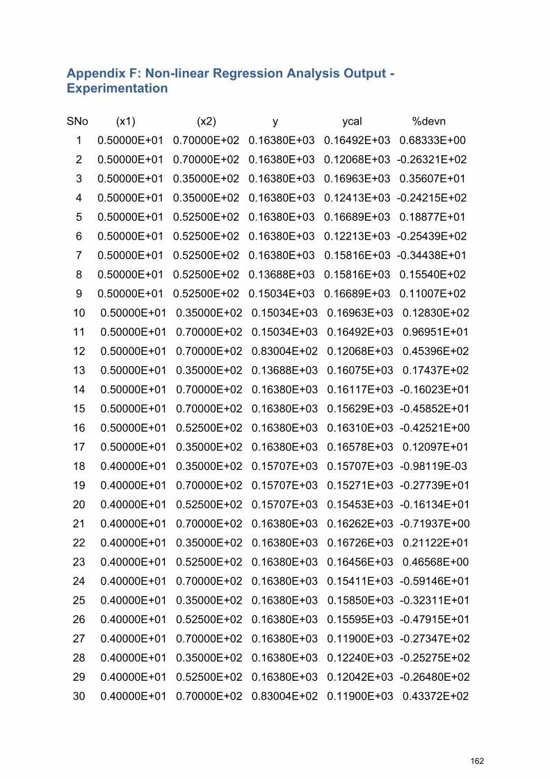
162

Appendix F: Non-linear Regression Analysis Output - Experimentation

SNo (x1) (x2) y ycal %devn

1 0.50000E+01 0.70000E+02 0.16380E+03 0.16492E+03 0.68333E+00

2 0.50000E+01 0.70000E+02 0.16380E+03 0.12068E+03 -0.26321E+02

3 0.50000E+01 0.35000E+02 0.16380E+03 0.16963E+03 0.35607E+01

4 0.50000E+01 0.35000E+02 0.16380E+03 0.12413E+03 -0.24215E+02

5 0.50000E+01 0.52500E+02 0.16380E+03 0.16689E+03 0.18877E+01

6 0.50000E+01 0.52500E+02 0.16380E+03 0.12213E+03 -0.25439E+02

7 0.50000E+01 0.52500E+02 0.16380E+03 0.15816E+03 -0.34438E+01

8 0.50000E+01 0.52500E+02 0.13688E+03 0.15816E+03 0.15540E+02

9 0.50000E+01 0.52500E+02 0.15034E+03 0.16689E+03 0.11007E+02

10 0.50000E+01 0.35000E+02 0.15034E+03 0.16963E+03 0.12830E+02

11 0.50000E+01 0.70000E+02 0.15034E+03 0.16492E+03 0.96951E+01

12 0.50000E+01 0.70000E+02 0.83004E+02 0.12068E+03 0.45396E+02

13 0.50000E+01 0.35000E+02 0.13688E+03 0.16075E+03 0.17437E+02

14 0.50000E+01 0.70000E+02 0.16380E+03 0.16117E+03 -0.16023E+01

15 0.50000E+01 0.70000E+02 0.16380E+03 0.15629E+03 -0.45852E+01

16 0.50000E+01 0.52500E+02 0.16380E+03 0.16310E+03 -0.42521E+00

17 0.50000E+01 0.35000E+02 0.16380E+03 0.16578E+03 0.12097E+01

18 0.40000E+01 0.35000E+02 0.15707E+03 0.15707E+03 -0.98119E-03

19 0.40000E+01 0.70000E+02 0.15707E+03 0.15271E+03 -0.27739E+01

20 0.40000E+01 0.52500E+02 0.15707E+03 0.15453E+03 -0.16134E+01

21 0.40000E+01 0.70000E+02 0.16380E+03 0.16262E+03 -0.71937E+00

22 0.40000E+01 0.35000E+02 0.16380E+03 0.16726E+03 0.21122E+01

23 0.40000E+01 0.52500E+02 0.16380E+03 0.16456E+03 0.46568E+00

24 0.40000E+01 0.70000E+02 0.16380E+03 0.15411E+03 -0.59146E+01

25 0.40000E+01 0.35000E+02 0.16380E+03 0.15850E+03 -0.32311E+01

26 0.40000E+01 0.52500E+02 0.16380E+03 0.15595E+03 -0.47915E+01

27 0.40000E+01 0.70000E+02 0.16380E+03 0.11900E+03 -0.27347E+02

28 0.40000E+01 0.35000E+02 0.16380E+03 0.12240E+03 -0.25275E+02

29 0.40000E+01 0.52500E+02 0.16380E+03 0.12042E+03 -0.26480E+02

30 0.40000E+01 0.70000E+02 0.83004E+02 0.11900E+03 0.43372E+02

163

31 0.40000E+01 0.52500E+02 0.83004E+02 0.12042E+03 0.45082E+02

32 0.40000E+01 0.35000E+02 0.16452E+03 0.16346E+03 -0.64166E+00

33 0.40000E+01 0.52500E+02 0.16452E+03 0.16082E+03 -0.22436E+01

34 0.40000E+01 0.70000E+02 0.16452E+03 0.15893E+03 -0.33969E+01

35 0.30000E+01 0.52500E+02 0.16380E+03 0.15315E+03 -0.64991E+01

36 0.30000E+01 0.52500E+02 0.83004E+02 0.11826E+03 0.42480E+02

37 0.30000E+01 0.52500E+02 0.12340E+03 0.15315E+03 0.24110E+02

38 0.30000E+01 0.35000E+02 0.12340E+03 0.15566E+03 0.26143E+02

39 0.30000E+01 0.52500E+02 0.16380E+03 0.16161E+03 -0.13363E+01

40 0.30000E+01 0.35000E+02 0.16380E+03 0.16426E+03 0.28059E+00

41 0.30000E+01 0.70000E+02 0.12340E+03 0.15134E+03 0.22645E+02

42 0.30000E+01 0.70000E+02 0.16380E+03 0.15970E+03 -0.25002E+01

43 0.30000E+01 0.70000E+02 0.83004E+02 0.11687E+03 0.40799E+02

44 0.30000E+01 0.70000E+02 0.16380E+03 0.15134E+03 -0.76021E+01

45 0.30000E+01 0.35000E+02 0.16380E+03 0.15566E+03 -0.49668E+01

46 0.30000E+01 0.52500E+02 0.16380E+03 0.15794E+03 -0.35761E+01

47 0.30000E+01 0.70000E+02 0.16380E+03 0.15608E+03 -0.47135E+01

48 0.30000E+01 0.35000E+02 0.16380E+03 0.16053E+03 -0.19959E+01

49 0.30000E+01 0.35000E+02 0.12340E+03 0.14705E+03 0.19165E+02

50 0.30000E+01 0.52500E+02 0.12340E+03 0.11826E+03 -0.41627E+01

51 0.30000E+01 0.35000E+02 0.12340E+03 0.12020E+03 -0.25921E+01

52 0.30000E+01 0.70000E+02 0.12340E+03 0.11687E+03 -0.52932E+01

53 0.20000E+01 0.35000E+02 0.15707E+03 0.13867E+03 -0.11714E+02

54 0.20000E+01 0.70000E+02 0.15707E+03 0.13483E+03 -0.14162E+02

55 0.20000E+01 0.52500E+02 0.15707E+03 0.13643E+03 -0.13137E+02

56 0.20000E+01 0.70000E+02 0.16380E+03 0.15568E+03 -0.49558E+01

57 0.20000E+01 0.35000E+02 0.16380E+03 0.16012E+03 -0.22450E+01

58 0.20000E+01 0.52500E+02 0.16380E+03 0.15754E+03 -0.38212E+01

59 0.20000E+01 0.70000E+02 0.16380E+03 0.14753E+03 -0.99292E+01

60 0.20000E+01 0.35000E+02 0.16380E+03 0.15174E+03 -0.73604E+01

61 0.20000E+01 0.52500E+02 0.16380E+03 0.14929E+03 -0.88541E+01

62 0.20000E+01 0.70000E+02 0.16380E+03 0.11393E+03 -0.30446E+02

63 0.20000E+01 0.35000E+02 0.16380E+03 0.11718E+03 -0.28463E+02

64 0.20000E+01 0.52500E+02 0.16380E+03 0.11529E+03 -0.29617E+02

164

65 0.20000E+01 0.70000E+02 0.83004E+02 0.11393E+03 0.37255E+02

66 0.20000E+01 0.35000E+02 0.83004E+02 0.11718E+03 0.41169E+02

67 0.20000E+01 0.52500E+02 0.83004E+02 0.11529E+03 0.38892E+02

68 0.20000E+01 0.35000E+02 0.16452E+03 0.15648E+03 -0.48813E+01

69 0.20000E+01 0.52500E+02 0.16452E+03 0.15396E+03 -0.64151E+01

70 0.20000E+01 0.70000E+02 0.16452E+03 0.15215E+03 -0.75190E+01

71 0.10000E+01 0.70000E+02 0.16380E+03 0.14904E+03 -0.90111E+01

72 0.10000E+01 0.35000E+02 0.16380E+03 0.15329E+03 -0.64160E+01

73 0.10000E+01 0.70000E+02 0.16380E+03 0.10906E+03 -0.33415E+02

74 0.10000E+01 0.35000E+02 0.16380E+03 0.11217E+03 -0.31516E+02

75 0.10000E+01 0.35000E+02 0.88419E+02 0.11019E+03 0.24627E+02

76 0.10000E+01 0.52500E+02 0.16380E+03 0.15082E+03 -0.79250E+01

77 0.10000E+01 0.52500E+02 0.16380E+03 0.11037E+03 -0.32620E+02

78 0.10000E+01 0.52500E+02 0.12340E+03 0.14292E+03 0.15822E+02

79 0.10000E+01 0.52500E+02 0.13688E+03 0.14292E+03 0.44125E+01

80 0.10000E+01 0.70000E+02 0.13688E+03 0.14124E+03 0.31808E+01

81 0.10000E+01 0.70000E+02 0.12340E+03 0.14124E+03 0.14455E+02

82 0.10000E+01 0.52500E+02 0.88419E+02 0.10842E+03 0.22617E+02

83 0.10000E+01 0.70000E+02 0.88419E+02 0.10714E+03 0.21171E+02

84 0.10000E+01 0.70000E+02 0.13688E+03 0.14904E+03 0.88781E+01

85 0.10000E+01 0.35000E+02 0.13688E+03 0.15329E+03 0.11983E+02

86 0.10000E+01 0.70000E+02 0.83004E+02 0.10921E+03 0.31570E+02

87 0.10000E+01 0.52500E+02 0.83004E+02 0.11037E+03 0.32965E+02

88 0.10000E+01 0.35000E+02 0.83004E+02 0.11217E+03 0.35144E+02

89 0.10000E+01 0.52500E+02 0.13688E+03 0.14292E+03 0.44125E+01

90 0.10000E+01 0.35000E+02 0.13688E+03 0.14527E+03 0.61236E+01

91 0.10000E+01 0.35000E+02 0.16380E+03 0.13723E+03 -0.16219E+02

92 0.10000E+01 0.52500E+02 0.16380E+03 0.13502E+03 -0.17570E+02

93 0.10000E+01 0.70000E+02 0.16380E+03 0.13343E+03 -0.18542E+02

94 0.10000E+01 0.35000E+02 0.12340E+03 0.13723E+03 0.11208E+02

95 0.10000E+01 0.52500E+02 0.12340E+03 0.13502E+03 0.94144E+01

96 0.10000E+01 0.70000E+02 0.12340E+03 0.13343E+03 0.81238E+01

97 0.10000E+01 0.35000E+02 0.16380E+03 0.14981E+03 -0.85405E+01

98 0.10000E+01 0.52500E+02 0.16380E+03 0.14739E+03 -0.10015E+02

165

99 0.10000E+01 0.70000E+02 0.16380E+03 0.14565E+03 -0.11077E+02

100 0.10000E+01 0.35000E+02 0.13688E+03 0.14981E+03 0.94412E+01

101 0.10000E+01 0.52500E+02 0.13688E+03 0.14739E+03 0.76766E+01

102 0.10000E+01 0.70000E+02 0.13688E+03 0.14565E+03 0.64065E+01

Regression Coefficients:

Non-linear regression

y = C * x1^a1 * x2^a2 * x3^a3 * ......

C = 93.00

a1 = 0.6290E-01

a2 = -0.3867E-01

a3 = 0.7982E-01

Number of Data Points = 102

Average deviation = 13.87 percent

Standard deviation = 18.71 percent

Note: In the above table

x1: Operating pressure

x2: Inlet fluid temperature

x3: Mass flux (not shown)

y: Heat flux from the experiment

ycalc: Heat flux calculated from the correlation developed.

%devn: Deviation in the calculated value (from correlation) and the experimental

value.

166

Appendix G: Non-linear Regression Analysis Output – Numerical Analysis

SNo x1 (x2) y ycal %devn

1 0.50000E+01 0.70000E+02 0.13056E+04 0.15463E+04 0.18442E+02

2 0.50000E+01 0.70000E+02 0.16380E+03 0.15244E+03 -0.69342E+01

3 0.50000E+01 0.35000E+02 0.22727E+04 0.18563E+04 -0.18319E+02

4 0.50000E+01 0.35000E+02 0.16380E+03 0.18300E+03 0.11722E+02

5 0.50000E+01 0.52500E+02 0.17891E+04 0.16706E+04 -0.66238E+01

6 0.50000E+01 0.52500E+02 0.16380E+03 0.16468E+03 0.53763E+00

7 0.50000E+01 0.52500E+02 0.15473E+04 0.11212E+04 -0.27540E+02

8 0.50000E+01 0.70000E+02 0.16380E+03 0.15244E+03 -0.69342E+01

9 0.50000E+01 0.35000E+02 0.11056E+04 0.12455E+04 0.12647E+02

10 0.50000E+01 0.70000E+02 0.10340E+04 0.10482E+04 0.13686E+01

11 0.30000E+01 0.52500E+02 0.10154E+04 0.85681E+03 -0.15622E+02

12 0.30000E+01 0.52500E+02 0.16380E+03 0.12586E+03 -0.23165E+02

13 0.30000E+01 0.52500E+02 0.12572E+04 0.12767E+04 0.15468E+01

14 0.30000E+01 0.35000E+02 0.15473E+04 0.14183E+04 -0.83420E+01

15 0.30000E+01 0.70000E+02 0.96709E+03 0.11819E+04 0.22214E+02

16 0.30000E+01 0.70000E+02 0.16380E+03 0.11651E+03 -0.28868E+02

17 0.30000E+01 0.70000E+02 0.91873E+03 0.79323E+03 -0.13660E+02

18 0.30000E+01 0.35000E+02 0.10638E+04 0.95184E+03 -0.10524E+02

19 0.10000E+01 0.70000E+02 0.67696E+03 0.66302E+03 -0.20596E+01

20 0.10000E+01 0.35000E+02 0.96709E+03 0.79560E+03 -0.17733E+02

21 0.10000E+01 0.70000E+02 0.83000E+02 0.65364E+02 -0.21249E+02

22 0.10000E+01 0.35000E+02 0.16380E+03 0.78427E+02 -0.52120E+02

23 0.10000E+01 0.35000E+02 0.41500E+02 0.68725E+02 0.65602E+02

24 0.10000E+01 0.52500E+02 0.82202E+03 0.71616E+03 -0.12878E+02

25 0.10000E+01 0.52500E+02 0.83000E+02 0.70597E+02 -0.14943E+02

26 0.10000E+01 0.70000E+02 0.43519E+03 0.44497E+03 0.22482E+01

27 0.10000E+01 0.52500E+02 0.48000E+02 0.61861E+02 0.28876E+02

28 0.10000E+01 0.70000E+02 0.83000E+02 0.57270E+02 -0.31000E+02

29 0.10000E+01 0.35000E+02 0.41500E+02 0.68725E+02 0.65602E+02

30 0.10000E+01 0.70000E+02 0.83000E+02 0.57270E+02 -0.31000E+02

167

31 0.40000E+01 0.35000E+02 0.11121E+04 0.10351E+04 -0.69319E+01

32 0.40000E+01 0.70000E+02 0.91873E+03 0.86257E+03 -0.61124E+01

33 0.20000E+01 0.35000E+02 0.33848E+03 0.39413E+03 0.16442E+02

34 0.20000E+01 0.70000E+02 0.29013E+03 0.32846E+03 0.13213E+02

35 0.40000E+01 0.52500E+02 0.10154E+04 0.93170E+03 -0.82463E+01

36 0.20000E+01 0.52500E+02 0.33848E+03 0.35478E+03 0.48165E+01

37 0.40000E+01 0.70000E+02 0.11605E+04 0.13751E+04 0.18493E+02

38 0.20000E+01 0.70000E+02 0.90088E+03 0.95483E+03 0.59889E+01

39 0.40000E+01 0.35000E+02 0.19342E+04 0.16501E+04 -0.14688E+02

40 0.20000E+01 0.35000E+02 0.14990E+04 0.11458E+04 -0.23565E+02

41 0.40000E+01 0.52500E+02 0.15473E+04 0.14853E+04 -0.40078E+01

42 0.20000E+01 0.52500E+02 0.10638E+04 0.10314E+04 -0.30492E+01

43 0.40000E+01 0.70000E+02 0.10154E+04 0.92288E+03 -0.91155E+01

44 0.20000E+01 0.70000E+02 0.72532E+03 0.64082E+03 -0.11650E+02

45 0.40000E+01 0.35000E+02 0.12089E+04 0.11074E+04 -0.83906E+01

46 0.20000E+01 0.35000E+02 0.87038E+03 0.76896E+03 -0.11653E+02

47 0.40000E+01 0.52500E+02 0.11121E+04 0.99685E+03 -0.10367E+02

48 0.20000E+01 0.52500E+02 0.82202E+03 0.69218E+03 -0.15795E+02

49 0.40000E+01 0.70000E+02 0.16380E+03 0.13557E+03 -0.17235E+02

50 0.20000E+01 0.70000E+02 0.83000E+02 0.94139E+02 0.13421E+02

51 0.40000E+01 0.35000E+02 0.16380E+03 0.16266E+03 -0.69478E+00

52 0.20000E+01 0.35000E+02 0.83000E+02 0.11295E+03 0.36088E+02

53 0.40000E+01 0.52500E+02 0.16380E+03 0.14642E+03 -0.10609E+02

54 0.20000E+01 0.52500E+02 0.83000E+02 0.10168E+03 0.22502E+02

55 0.10000E+01 0.70000E+02 0.83000E+02 0.66000E+02 -0.20483E+02

56 0.40000E+01 0.70000E+02 0.16380E+03 0.13557E+03 -0.17235E+02

57 0.20000E+01 0.70000E+02 0.83000E+02 0.94139E+02 0.13421E+02

58 0.50000E+01 0.52500E+02 0.16380E+03 0.16468E+03 0.53763E+00

59 0.10000E+01 0.52500E+02 0.83000E+02 0.70597E+02 -0.14943E+02

60 0.50000E+01 0.35000E+02 0.16380E+03 0.18300E+03 0.11722E+02

61 0.10000E+01 0.35000E+02 0.83000E+02 0.78427E+02 -0.55100E+01

62 0.30000E+01 0.35000E+02 0.16380E+03 0.13981E+03 -0.14644E+02

63 0.10000E+01 0.52500E+02 0.48354E+03 0.48064E+03 -0.59998E+00

64 0.10000E+01 0.35000E+02 0.48354E+03 0.53395E+03 0.10425E+02

168

65 0.20000E+01 0.35000E+02 0.83000E+02 0.11295E+03 0.36088E+02

66 0.20000E+01 0.52500E+02 0.83000E+02 0.10168E+03 0.22502E+02

67 0.40000E+01 0.35000E+02 0.16380E+03 0.16266E+03 -0.69478E+00

68 0.40000E+01 0.52500E+02 0.16380E+03 0.14642E+03 -0.10609E+02

69 0.50000E+01 0.70000E+02 0.11466E+04 0.13042E+04 0.13747E+02

70 0.50000E+01 0.52500E+02 0.16380E+04 0.14087E+04 -0.13995E+02

71 0.50000E+01 0.35000E+02 0.19246E+04 0.15650E+04 -0.18686E+02

72 0.50000E+01 0.70000E+02 0.53234E+03 0.68035E+03 0.27803E+02

73 0.50000E+01 0.52500E+02 0.65519E+03 0.73488E+03 0.12163E+02

74 0.50000E+01 0.35000E+02 0.77804E+03 0.81639E+03 0.49288E+01

75 0.40000E+01 0.70000E+02 0.10647E+04 0.11597E+04 0.89243E+01

76 0.40000E+01 0.52500E+02 0.13104E+04 0.12526E+04 -0.44061E+01

77 0.40000E+01 0.35000E+02 0.15561E+04 0.13497E+04 -0.13262E+02

78 0.40000E+01 0.70000E+02 0.40949E+03 0.60497E+03 0.47737E+02

79 0.40000E+01 0.52500E+02 0.49139E+03 0.65345E+03 0.32980E+02

80 0.40000E+01 0.35000E+02 0.53234E+03 0.70409E+03 0.32262E+02

81 0.30000E+01 0.70000E+02 0.94183E+03 0.99677E+03 0.58336E+01

82 0.30000E+01 0.52500E+02 0.11056E+04 0.10767E+04 -0.26202E+01

83 0.30000E+01 0.35000E+02 0.12694E+04 0.11961E+04 -0.57776E+01

84 0.30000E+01 0.70000E+02 0.40949E+03 0.51997E+03 0.26980E+02

85 0.30000E+01 0.52500E+02 0.45044E+03 0.56165E+03 0.24689E+02

86 0.30000E+01 0.35000E+02 0.49139E+03 0.62395E+03 0.26976E+02

87 0.20000E+01 0.70000E+02 0.81899E+03 0.80525E+03 -0.16773E+01

88 0.20000E+01 0.52500E+02 0.98278E+03 0.86979E+03 -0.11497E+02

89 0.20000E+01 0.35000E+02 0.11466E+04 0.96627E+03 -0.15726E+02

90 0.20000E+01 0.70000E+02 0.32759E+03 0.42007E+03 0.28229E+02

91 0.20000E+01 0.52500E+02 0.36854E+03 0.45373E+03 0.23117E+02

92 0.20000E+01 0.35000E+02 0.40949E+03 0.50406E+03 0.23096E+02

93 0.10000E+01 0.70000E+02 0.49139E+03 0.55915E+03 0.13790E+02

94 0.10000E+01 0.52500E+02 0.57329E+03 0.60397E+03 0.53516E+01

95 0.10000E+01 0.35000E+02 0.73709E+03 0.67097E+03 -0.89710E+01

96 0.10000E+01 0.70000E+02 0.20475E+03 0.29169E+03 0.42460E+02

97 0.10000E+01 0.52500E+02 0.28665E+03 0.31507E+03 0.99132E+01

98 0.10000E+01 0.35000E+02 0.28665E+03 0.35001E+03 0.22104E+02

169

Regression Coefficients:

Non-linear regression

y = C * x1^a1 * x2^a2 * x3^a3 * ......

C = 17.05

a1 = 0.5262

a2 = -0.2489

a3 = 0.5922

Number of Data Points = 98

Average deviation = 16.15 percent

Standard deviation = 20.59 percent

170

Appendix H: Sample Calculation of CHF from Experimental Correlation This section describes calculation procedure to determine the CHF using experimental

correlation developed from current investigations. A point is considered which was not

used during the experimental investigations to perform the sample calculation.

P = 1.5 bar

Tin = 60oC

G = 1000 kg/m2s Based on the experimental investigations, the CHF correlation developed is given

below.

𝒒𝑪𝑯𝑭,𝑫𝒓𝒆𝒇

= 𝟗𝟑 ∗ 𝑷𝟎.𝟎𝟔𝟐𝟗 ∗ 𝑻𝒊𝒏−𝟎.𝟎𝟑𝟖𝟔𝟕 ∗ 𝑮𝟎.𝟎𝟕𝟗𝟖𝟐

By substituting the P, Tin and G in the above equation, critical heat flux obtained at reference tube diameter of 8 mm (OD) is 142 kW/m2

171

Appendix I: Publications from Current Investigations

1. Rajeshwar Sripada, Siva Subrahmanyam Mendu, Divyasree Tentu, Shanmukh

Simhadri Varanasi, 2020, “Development of Correlation for Critical Heat Flux for

Vertically Downward Two-Phase Flows in Round Tubes.” Published online 15 May

2020 in Experimental Heat Transfer.

DOI: https://doi-org/10.1080/08916152.2020.1760963.

2. Rajeshwar Sripada, Veeredhi Vasudeva Rao, 2017, “Review of Critical Heat Flux in a

Vertically Downward Two Phase Flows.” Proceedings of 24th National and 2nd

International Heat and Mass Transfer Conference (IHMTC-2017), BITS Pilani,

Hyderabad, India, pp:2097-2102; ISBN: 978-1-56700-478-6. DOI: https://doi-

org/10.1615/IHMTC-2017.2940.

3. Sumanth Theeda, Siva Subrahmanyam Mendu, Rajeshwar Sripada, Veeredhi

Vasudeva Rao, 2018, “Numerical Analysis of Critical Heat Flux During Sub-Cooled

Boiling for a Vertically Downward Flow.” Proceedings of Fifth International Conference

on Computational Methods for Thermal Problems (THERMACOMP2018), Indian

Institute of Science, Bangalore, India, pp: 846-850. ISSN: 2305-6924.

4. Rajeshwar Sripada, Subaschandar N, Veeredhi Vasudeva Rao, (2019), “Numerical

Analysis of Critical Heat Flux for Vertically Upward and Downward Flows in Circular

Pipe Sections.” Proceedings of International Conference on Design, Materials,

Cryogenics and Constructions (ICDMC-2019), Veltech University, Chennai, India, to

be published online in Lecture Notes in Mechanical Engineering by Springer in June

2020, pp: yet to assign, ISBN: 978-981-15-3631-1; ISSN: 2195-4356; DOI:

https://doi.org/10.1007/978-981-15-3631-1.

5. Rajeshwar S., Siva Subrahmanyam M., Vasudeva Rao V., (2020). “Development of

Critical Heat Flux Correlation in Circular Pipe Sections with Vertically Downward Two-

Phase Flows by Numerical Analysis and Comparison with Experimental Correlation.”

Proceedings of the ASME 2020 International Mechanical Engineering Congress and

Exposition - IMECE-2020, Portland, USA. ISBN: 978-0-7918-8459-1. DOI: https://doi-

org/10.1115/IMECE2020-23850.

Full Terms & Conditions of access and use can be found athttps://www.tandfonline.com/action/journalInformation?journalCode=ueht20

Experimental Heat TransferA Journal of Thermal Energy Generation, Transport, Storage, andConversion

ISSN: 0891-6152 (Print) 1521-0480 (Online) Journal homepage: https://www.tandfonline.com/loi/ueht20

Development of correlation for critical heat fluxfor vertically downward two-phase flows in roundtubes

Rajeshwar Sripada, Siva Subrahmanyam Mendu, Divyasree Tentu,Shanmukh Simhadri Varanasi & Vasudeva Rao Veeredhi

To cite this article: Rajeshwar Sripada, Siva Subrahmanyam Mendu, Divyasree Tentu, ShanmukhSimhadri Varanasi & Vasudeva Rao Veeredhi (2020): Development of correlation for critical heatflux for vertically downward two-phase flows in round tubes, Experimental Heat Transfer

To link to this article: https://doi.org/10.1080/08916152.2020.1760963

Published online: 15 May 2020.

Submit your article to this journal

View related articles

View Crossmark data

Development of correlation for critical heat flux for verticallydownward two-phase flows in round tubesRajeshwar Sripadaa, Siva Subrahmanyam Mendub, Divyasree Tentub,Shanmukh Simhadri Varanasib, and Vasudeva Rao Veeredhia

aDepartment of Mechanical and Industrial Engineering, University of South Africa, Johannesburg, South Africa;bDepartment of Mechanical Engineering, Maharaja Vijayaram Gajapathi Raj College of Engineering (A),Vizianagaram, India

ABSTRACTCritical Heat Flux (CHF) is one of the catastrophic failure modes encoun-tered in two-phase flows in nuclear, chemical, and power industries.Considerable research was carried on CHF in last few decades in horizontal,inclined, and vertically upward flows. Only limited information, mostly atatmospheric pressure conditions and including CHF enhancers like inletthrottling, was available on CHF in vertical pipes with flow directed down-wards. The complexity associated with vertically downward two-phaseflows, due to flow instabilities and premature tube burnout, dictates forstringent design considerations, especially, from CHF perspective. Asa result, accurate estimation of CHF is a requirement not only from perfor-mance, but also more significantly from safety perspective. The objective ofthis paper is to develop a correlation for CHF in vertical tubes in which thefluid flow was directed downward. As part of these investigations,a versatile test rig was designed and developed. Experiments were con-ducted in the pressure range of 1 to 5 bar and a CHF correlation is proposedas a function of inlet fluid temperature, mass flux and pressure in theabsence of inlet throttling or other similar effects. The new correlationdeveloped agrees well with the data from current experiments witha mean deviation of 13.87% and standard deviation of 18.71%. The uncer-tainty analysis revealed a 90% confidence level on the CHF estimate due tovariation in the input variables.

ARTICLE HISTORYReceived 1 February 2020Accepted 21 April 2020

KEYWORDSCritical heat flux; verticallydownward flow; two-phaseflows; boiling; non-linearregression analysis; CHFcorrelation

Introduction

Research in the field of two-phase flows has been active for more than last six decades. Themain emphasis of these investigations was to understand the tube failure due to departurefrom nucleate boiling (DNB) or reaching the critical heat flux (CHF) limits. Emphasis was alsoplaced to determine the void fraction and to develop the flow pattern maps. Most of theseinvestigations were conducted in tubes that were oriented in the upright straight tubes withflows directed in upward direction. There were many investigations in which two-phase flowswere also considered in horizontal and inclined tubes. For the two-phase flows in horizontaltubes, the direction of fluid flow has minimum affect while the direction of fluid flow canaffect the CHF significantly in vertical and inclined tubes. Although, most of the two-phaseflow equipment design falls into one of the flow orientations mentioned above, there arenumerous situations in which the flow would happen in vertical tubes with the fluid flowing inthe downward direction in the tube. The U tube sections of the boilers and the two-phase flow

CONTACT Rajeshwar Sripada rajeshwar33482@gmail.com Department of Mechanical and Industrial Engineering,University of South Africa, Cnr Christiaan de Wet & Pioneer Avenue, Florida, Private Bag X6 Florida, Johannesburg, 1710, SouthAfrica© 2020 Taylor & Francis

EXPERIMENTAL HEAT TRANSFERhttps://doi.org/10.1080/08916152.2020.1760963

heat exchangers used in conventional and combined cycle power plants, the cryogenic coolingsystem used in the spacecrafts, the boilers and the syngas coolers used for high pressure steamgeneration in the chemical applications like gasification plants, the steam generators used inthe nuclear industry are some of the examples where the two-phase flows in vertically down-ward direction. However, the same levels of investigations in down flow were not carried ascompared to the other flow orientations. The complexity associated with two-phase flowinstabilities, especially at low pressures and low flow rates, leads to premature tube burnout. The buoyancy dominates at low flow rates and at very low pressures, allowing the bubblesto rise faster in upward direction. The inability of the liquid momentum traveling in down-ward direction to suppress the rise velocity of the bubble results in significant amount of vaporaccumulation, especially at the inlet. All these factors contribute to increased level of risks intwo-phase flows directed vertically downwards. Most of the researchers, previously, tried tounderstand the differences in void fraction estimates and the flow patterns associated with theflows directed vertically downwards and compared the same with flows directed verticallyupwards. Bhagwat [1] compiled the investigations carried on flow pattern maps and the voidfraction in two-phase flows directed vertically downwards. The research on the tube failure dueto CHF and DNB in downward flows did not find the same level of attention compared to theother flow orientations. The CHF correlations available in open literature for the flowsdirected downwards in upright tubes were limited in number and were mostly published atthe atmospheric pressure conditions. Further, the CHF correlations published included theeffects of inlet throttling and plenum effects, which reduce the CHF risk significantly. Incomparison, the CHF correlations available for the flows in inclined tubes, horizontal tubesand tubes with vertically upward flow were plenty, covering a broad range of geometric andprocess conditions as compiled by Hall and Mudawar [2, 3].

Papell et al. [4] conducted experiments with liquid nitrogen in the pressure range of 3.5 and16.5 bar for both up and down flows in a round tube. However, they did not develop any CHFcorrelation. Their main observation was that the buoyancy force was stronger at velocities lessthan 0.61 m/s, causing the bubbles to ascend against the liquid flow that resulted in accumula-tion of vapor at the inlet leading to two-phase flow instabilities. Blumenkrantz et al. [5] andCumo et al. [6] observed upflow CHF to be many times higher than downflow CHF at verylow mass flow rates of water but did not develop any CHF correlation for flows directedvertically downwards. Mishima et al. [7, 8] performed extensive investigations on verticallydownward two-phase flows considering geometric effects that include round tubes, rectangularchannels, internally heated annulus at atmospheric conditions. Primarily they focused on lowflow velocities, flow stagnation and flow reversal scenarios in which inlet throttling, upstreamcompressibility and buoyancy effects are included. Two-phase flow instabilities and other keyCHF characteristics were reported in detail for vertically downward two-phase flows, especiallyfor the cases with inlet throttling and plenum. They also concluded that the upflow CHF washigher than downflow CHF at low mass fluxes but the difference becomes negligible at highmass fluxes.

Sudo et al. [9, 10] conducted experiments in two different rectangular channel geometries forvertically up and down flow directions at pressure close to atmospheric pressure. The main emphasiswas given on DNB heat flux. They also concluded that the flow direction had no impact on heat fluxat both low and high mass fluxes but the DNB heat flux was much lower for downward flows atintermediate flow rates. Based on their experiments, they reported a new countercurrent flowlimitation correlation to predict the CHF given by Eq. (1). They compared the correlation withtheir own experimental data as well with the correlation proposed by Mishima [11], which is givenby Eq. (2).

2 R. SRIPADA ET AL.

q�CHF ¼ AAH

CpΔTsub

hlv

� �G� þ 1

1:52

� �2 aλ

� �0:5F2:875

" #(1)

q�CHF ¼ AAH

CpΔTsub

hlv

� �G� þ C2 A

AH

� � ffiffiaλ

p1þm ρv

ρl

� �1=4� �2 (2)

Where G* is the dimensionless mass flow rate described by Eq. 3.

G� ¼ G=

ffiffiffiffiffiffiffiffiffiffiffiffiffiffiffiffiffiffiffiffiffiffiffiffiffiffiffiffiλγg γl � γg

� �g

r(3)

They also provided the information related to some of the previous investigations carried onvertically downward two-phase flows with geometric details as described in Table 1.

The characteristics of CHF in round tubes for two-phase flows directed downwards, includinginlet throttling and plenum effects up to pressures of 7 bar were investigated by Ruan et al. [12]. Twokinds of CHF behavior was observed by them. The first type termed as flooding type CHF termed asCHF1 was due to the combination of the buoyancy and the compressibility acting at upstream on thebubble opposite to the direction of the flow. The second one could be interpreted as dry-out andtermed as CHF2 and was observed at high heat fluxes. Chang et al. [13] developed CHF correlationsbased on non-dimensional mass flux G* by conducting experiments in stainless-steel round tubes atatmospheric pressure in vertically downward two-phase flows. They concluded that the inletthrottling is required to maintain stable flow for two-phase flows directed vertically downward.They also proposed CHF correlations for low and high G* that are given by Eq. (4) and Eq. (5),respectively. The smaller of qcH and qcL should be considered as CHF value.

q�cL ¼ q�cF þ 0:01351 D�ð Þ�0:473 lD

� ��0:533

G�j j1:45 (4)

q�cH ¼ q�cF þ 0:05664 D�ð Þ�0:247 lD

� ��0:501

G�j j0:770 (5)

Atul et al. [14] conducted experiments to understand the thermal impact and the dynamics ofa vapor bubble in vertically downward and upward flows. They had visualized the bubble growth anddetachment from the heater surface and observed substantial differences in bubble trajectory afterdeparture from the nucleation site for both the flow configurations. Experiments were conducted byAroonrat et al. [15] in corrugated tubes with flow directed vertically downward with differentcorrugation pitches to understand the pressure drop and the evaporative heat transfer of refrigerantR-134a. The heat transfer coefficient (HTC), and the frictional pressure drop was found to be higherin corrugated tubes when compared with the experiments conducted in smooth tubes.

Table 1. Previous investigations carried on vertically downward flow and as presented in article by Sudo et al. [9].

Author Pressure (bar) Mass Flux (kg/m2 s)Inlet Condition

(oC) Geometry/Cross Section

Yucel et al. 1.6 60–1200 ΔTin = 58–97 Rectangular,Kirby et al. 1.8 637–2700 ΔTin = 3–32 AnnularMishima et al. 1 0–600 Tin = 29–87 RectangularMishima et al. 1 0–1130 Tin = 30–60 Circular

EXPERIMENTAL HEAT TRANSFER 3

Shen et al. [16] performed experiments at pressures close to critical and sub-critical pressures andprovided good insights of the characteristics of HTC in flows directed in vertically downwarddirection. They also compared the HTCs with the vertically upward two-phase flows and concludedthat HTCs at such high pressures are comparable. Mohammed et al. [17] conducted experiments invertically upward and downward flows in circular cylinders to understand the mixed convection heattransfer for laminar flows. They reported that the surface values were higher for flows directeddownwards when compared to flows directed upwards but were lower than the horizontal flows.A detailed report on existing CHF correlations and HTC characteristics for vertically downwardflows was compiled by Rajeshwar et al. [18].

To summarize, only a few CHF correlations are available for vertically downward two-phase flowsin comparison to vertically upward two-phase flows. Most of these correlations were developed atatmospheric conditions using air-water mixture, liquid nitrogen and freons considering differentgeometries like round tubes, rectangular channels and internally heated annulus tubes. No signifi-cant data is available for steam-water mixtures at high pressures, the scenario, which is commonlyfound in real time power plants, chemical industries etc. Further, the previous investigators used DCpower supply with plate heating or direct pipe heating, which could bring in additional risks of non-uniform heating, which was not discussed in detail by previous investigators. Most of the previousinvestigations included the effects of inlet throttling or the plenum to determine the CHF, whichdecreases the CHF risk significantly. On the other hand, the absence of inlet throttling or inletplenum could constitute the other extreme end where the CHF risk would be significant, thusallowing to create bounds in which the CHF value could exist. All these factors gave an opportunityto make suitable design modifications to the test rig and to enhance the predictions of CHF,especially for flows directed vertically downwards.

In the current investigations, a test rig was built to conduct the experiments for water steam two-phase flows in vertically downward direction up to pressures of 5 bar. A few important designmodifications were made to the current test rig in comparison to previous test rigs used by otherinvestigators. Safety was given importance while designing and developing the test rig. Proving runswere conducted on the test rig with previously published conditions and the results were comparedto establish the credibility of the test rig. A Design of Experiments (DOE) matrix was generated andexperiments were conducted to develop a CHF correlation up to pressures of 5 bar in a verticallydownward two-phase flow.

Experimental setup

This section discusses the experimental test setup that was designed and developed as a part of thepresent investigation with suitable design modifications to improve the predictions. The basic sketchof the experimental test rig is shown in Figure 1.

Test section

The test section includes 6 heaters (H1-H6), each 160 mm in height and with a heater rating of 2 kWmaximum. The heaters are connected to AC power source through the voltage regulators (variacs).The heating elements were made of Kanthal wire wounded to a ceramic cylindrical structure with8 mm through hole in the center in the axial direction. The ceramic with the heating element wascovered by thick insulation made of glass wool (~30 mm thick) and enclosed in a steel cylinderstructure, closed from all the directions, except for the through hole. It ensures that there isminimum heat loss from the system to the surroundings. The maximum heat loss to the surround-ings was observed to be less than 15% at the maximum heater output of 12 kW and decreases withdecrease in heater output to below 1%.

The test pipe was made of SS304 material, 6 mm inner diameter, 1 mm thick and 1000 mm long.The pipe was inserted through the hole provided in the center of the ceramic structure with a close

4 R. SRIPADA ET AL.

fit with a negligible clearance between the test pipe and the ceramic structure. A small gap ofapproximately 6 mm was maintained in between two heaters to incorporate thermocouples (TC1-TC14) as shown in Figure 1, with two thermocouples placed in opposite direction at the sameelevation. The gaps were filled with Glass wool insulated material to minimize the heat losses to thesurroundings. All the thermocouples were connected separately to each of the displays (D1-D14).The displays were enclosed in display units 1 and 2. Each heater was connected to a separate variabletransformer (VT1-VT6) to regulate the power input and thereby vary the heat input during theexperiments. Each of the heater’s resistance was measured before commissioning and the suitablecorrection factor was included to achieve constant heat input through all the heaters uniformly. Theentire test section was fixed on a rigid stand to give additional support for both the heaters and to thethermocouples attached to the test section.

Test loop

The entire test section connects to an external circuit that consists of water reservoir, pump,a network of pipes, flow-regulating valves, flow measuring devices, pressure gauges, temperaturemeasuring devices and a sink. The reservoir tank W1 acts like a source with water being taken fromthe external source and preheating of water done with external heaters to the desired inlet tempera-ture. A high-performance high temperature durable pump was used for the experiments. The pumpwas manufactured by GRUNDFOS Inc. (Denmark) and can handle fluids up to a temperature of 90°C. It was a 1HP pump with a rated flow of 3.1 m3/h, operates on a 3-phase power supply and has6impeller. The piping network consists of various sizes of pipes gradually decreased from 25NPS

Figure 1. Schematic of experimental rig used in current investigations.

EXPERIMENTAL HEAT TRANSFER 5

(SCH10) at pump outlet to 15NPS (SCH10) to 8NPS (SCH40) to the 8 mm outer diameter test pipe.The piping network lines were also checked for minimum thickness requirement using ASME B31.3[19] code. The exit from the test section bifurcates to two lines. The first line gets connected to thereservoir W1 to get a closed loop circuit and used for preheating of the water instead of using heatersor to cool the heaters post experiment. The second line ends in reservoir W2, which was used duringthe experiments for flow rate and the temperature measurement of the water at the exit. The flowrate and the pressure can be regulated using a set of valves (V1-V5) as shown in Figure 1.

Instrumentation

Two different mechanisms were used to measure the flow rate to the test section. A rotameter (F1)was placed slightly above the pump discharge to measure the volumetric flow rate. The rotameterwas designed to withstand the fluid temperature up to 100°C. The rotameter was calibrated, andappropriate correction curves were included for setting the flow rate at different operating condi-tions before using it. Provision was also made to measure flow rate manually at the exit in ReservoirW2 using measuring jar and the stopwatch to ensure the consistency in the measurements with therotameter. Three independent measurements were taken at the starting of each experiment and theflow rates were compared between rotameter and the manual measurement. Analog type thermo-meters were placed at different locations with long stems to measure the temperature of the fluid atvarious locations. Analog type pressure gauges (P1-P3) were placed at different locations to measurethe pressure during the experiments. K-type thermocouples were used to determine the metaltemperatures of the test pipe. Each thermocouple was calibrated before installing it on the testsection. An independent digital K-Type probe with a resolution of 0.1°C was used to calibrate thethermocouples. The analog thermometers were also calibrated before the usage to ensure theaccuracy in the readings or to include appropriate correction factors. Table 2 shows the range,resolution and accuracies of the instruments used in current experiments.

Test procedure

The entire setup was assembled and checked for any possible leakages. Hydrotest was conducted ata pressure of about 6 bar to detect the leakages, if any, through the entire system before conductingthe scheduled experiments. The hydrotest was conducted as per the procedure listed in ASME B31.3for a period of 20 min.

The water in the reservoir W1 was preheated to required temperature, the pumps were switchedon, the flow rate and the required pressures were achieved by regulating the valves V2 and V4 whileclosing the valve V3. Once the desired flow rate, and the pressure was achieved, the heaters wereswitched on. The voltages in the variable transformer were adjusted to account for differentresistances of each of the heater and thereby ensure uniform heating of the entire test section. Thetemperatures recorded by the thermocouples were continuously monitored for temperature excur-sions or abrupt rise in metal temperature up to a metal temperature of 400°C. The temperature limitof 400°C was set as a safety measure based on reduction in mechanical properties of SS304 below450–500°C as per ASME B31.3. Some of the previous investigators set the temperature limit of 400°C

Table 2. Specifications of the instruments.

Parameter Instrument Range/Resolution Accuracy

Pressure Pressure Gauge 0–7 bar/0.1 bar ±0.2 barFlow Rate Rotameter 0–7 LPM/0.1 LPM ±1.5%Inlet Fluid Temperature K-type probe 300°C/0.1°C ±1oCMetal Temperature Chromel-Alumel Thermocouples 1260°C/0.1°C ±1oCFluid Temperature Long stem thermometer probes 300°C/1°C ±2oCPower Input/Voltage Variac 240 V/2 V ±2 V

6 R. SRIPADA ET AL.

for SS304 test material and quoted the abrupt rise in metal temperature after 250°C as the CHF point[12, 13]. The same approach was used in current investigations. The heater controller was set to thispre-set temperature of 400°C at which the heaters would be shut off. Additional temperaturemeasurements were taken on the heater surface to determine the losses to the surroundings. Theflow rate at the exit was evaluated at a frequency of every 2 min and corresponding fluid tempera-tures were also determined for each run. The test section was cooled using a combination of anexternal source and pumping the cold water through the circuit from Reservoir W1 and routing backthe same to Reservoir W1. Once the test section temperature reached to the ambient temperature,the next experiment was conducted.

Proving runs

This section discusses the results based on the current investigations including the proving runs,development of CHF correlation and comparison with the existing correlations available in openliterature.

Figure 2 shows the comparison based on the proving runs conducted for current experimentaltest rig with the work done by Mishima et al. [7, 8]. The diameter of the tube used in both theexperiments was the same and the process conditions were replicated to have one to one compar-ison. The previous investigations were conducted with a system that includes inlet throttling andplenum. The results from the current experiment shows that the CHF value at low flow rate of 50 kg/m2 s was comparable with the data published by Mishima et al. with inlet throttling. However, therewas an abrupt increase in the CHF limit for Mishima et al. at flow rates greater than 50 kg/m2 s,significantly attributed to inlet throttling. The curves flatten out beyond 200 kg/m2 s based onMishima et al. and the same trend was observed from the current test runs but at lower heat fluxvalues. The same trends were not observed for the current investigations when compared with theresults reported by Mishima et al. [7] with test section consisting of plenum. This case showsrelatively low CHF at mass fluxes of 400 kg/m2 s when compared with the current investigations.The CHF value reported by Mishima et al. increases abruptly after the 400 kg/m2 s and found to bewell above the CHF value determined from current investigations as shown in Figure 2. The valuesreported by Mishima et al. eventually tends to reach to CHF with inlet throttling values as providedby Mishima et al. at very high mass fluxes. The upper plenum case acts like a source to inducepressure-drop oscillations due to effective upstream compressibility resulting in lower CHF values.The abrupt increase in CHF value was attributed to the velocity exceeding the critical value to

Figure 2. Proving run for results from current test rig compared with work by Mishima et al. [7].

EXPERIMENTAL HEAT TRANSFER 7

stagnate ascending of the bubbles. The difference at low mass fluxes was found to be even lower than50% for the plenum case when compared to current investigations. All the comparisons were madeat same Lcritical values from previous investigations and for same critical quality to have similarcomparisons. For low flow rates, the current experiments shown complete steam at the exit and is inagreement with the trends reported by Mishima et al. [7, 8]. Further, the CHF was observed atdifferent locations anywhere along the length of the tube and depending on the process conditions,especially the mass flux. This is in line with some of the observations made from the previousinvestigators [12, 13].

Figure 3 shows the thermocouple reading of one of the thermocouples that measures the outermetal temperature for one of the proving runs. The metal temperature shoots up after 24 min andcrosses the preset metal temperature of 400°C for the proving run indicating the potential CHF risk.

Similar proving runs were conducted with the experiments conducted by Chang et al. [13]. Figure4 shows the comparison of the results between experiments conducted by the Chang et al. and thecurrent investigations with same process conditions. As observed from previous proving rundiscussion based on Mishima et al., the current run also shows 3–4 times lower CHF value comparedto the previous investigations. Chang et al. reported very large inlet throttling, much higher thanMishima et al. [7], resulting in even much higher CHF value at low mass fluxes and hence significantdifference in the predictions.

Consistency checks were also made for current investigations by repeating a few data points atmaximum, average and minimum mass fluxes and comparing the results between the two runs. The

Figure 3. Thermometer reading for the proving run with Mishima et al. [7].

Figure 4. Proving run for current test rig compared with work by Chang et al. [12].

8 R. SRIPADA ET AL.

results between two runs were comparable with a maximum difference of ~2% observed between theruns.

Previous investigators did not explicitly describe the impact of CHF without inlet throttling andplenum. At this stage, further literature search was carried to understand the impact of theseparameters on the CHF. Mayinger et al. [20] conducted extensive investigations on two-phaseflows to understand the effect of inlet throttling and the twisted tapes on the CHF. They alsomade comparison with the cases where the throttling and the twisted tape were absent. Theseinvestigations were carried with water in the pipes with diameter of 7–15 mm and at pressures of 68to 137 bar. Their investigations revealed that the pulsating burnout, common in sub-cooled flowboiling, shows a CHF values close to 20-50% lower than those obtained with the hydrodynamicallystable flow. CHF was increased by almost 80% with the inclusion of inlet throttling and twisted tapes.The smaller L/D ratios of 5–10 shown even greater influence compared to L/D of 80–100 or more.The proving runs showed that the CHF values were an order of magnitude lower than the previousinvestigations. It was attributed to all the factors listed by Mayinger et al. including the absence of theinlet throttling or the twisted tape and larger L/D ratios of the order of 160 in current investigationsas compared to Mishima et al. with a L/D ratio of ~60. While the observations by Mayinger et al.were at high pressures, the impact of all the above said parameters could be profound at lowerpressures, close to atmosphere, and could potentially lead to much higher deviations in the currentinvestigations.

A few more checks were also performed and compared with the experimental results from theprevious investigations before conducting the final runs for correlation development. As most of theauthors reported out, flow instabilities at low mass fluxes and at atmospheric pressure was observedfrom current investigations. The conclusion was drawn based on the variations in the measurementof the volumetric flow rate at the exit and the fluctuation of maximum temperature location from thethermocouple readings. Figure 5 shows the metal temperature for two consecutive thermocouples forlow mass flux and atmospheric pressure case. The thermocouples showed a periodic fluctuation inthe metal temperature but never reached 250°C or the CHF preset limit of 400°C. The temperaturemeasurement showed an offset in the measurement in between the consecutive thermocouples,indicating the possible slug flow regime and oscillation of the slug. The flow at the exit observed wasvapor with pockets of liquid water coming out at small intervals. These flow instabilities had reducedfor the same low mass fluxes but at higher pressures due to reduced liquid to vapor ratio.

Figure 6 shows the estimated average void fraction as a function of pressure and for maximumthroughput (~3000 kg/m2 s) and minimum throughput (58 kg/m2 s) and for maximum and

Figure 5. Consecutive thermocouple measurements at 1 bar showing possible fluctuations.

EXPERIMENTAL HEAT TRANSFER 9

minimum inlet fluid temperatures of 70 and 35°C, respectively. The results are shown for 3.5 kWheat input condition.

The average void fraction was estimated using the empirical correlations available in openliterature by Saha et al. [21] and given by Eq. (6). The average void fraction was estimated at theexit using the current experimental values by measuring the fluid exit temperature, flow rate, heatinput, pressure and other parameters and excluding the pressure drop. The sub-cooled flow boilingcalculations were included as recommended by Saha et al. [21]. A distribution parameter (Co) of 0.85for vertically downward two-phase flows was used for all the calculations and as proposed by Ishii[22]. While correct estimation of Co and void fraction plays an important role, the results for basicchecks shown below were based on available open literature information and should be treated onlyas qualitative trends.

ε ¼ x

Co x � ρl�ρgρl

� �þ ρg

ρl

h iþ ρg � vgj

G

h ih i24

35 (6)

From Figure 6, for low mass flux, the average void fraction marginally increases with increase in inletfluid temperature. At high mass fluxes, the inlet water temperature had negligible effect on theaverage void fraction. At low mass fluxes and at atmospheric pressure, the average void fractionestimated was 100%. The experiments had shown complete vapor at the exit, validating the abovetrends, especially at atmospheric pressure. The inlet fluid temperature had minimum effect even atlow mass flow rates. This observation was in agreement with some of the data published by previousinvestigators [7–11].

Figure 7 shows the onset of nucleate boiling estimation based on the current experimental results.The empirical correlation given by Bergles and Rohsenow and as given in Mostafa Ghiaasiaan [23]was used for the calculations. Equation (7) shows the ONB empirical correlation used for the currentcalculations.

Tw � Tsatð ÞONB ¼ 0:556qw

1082P1:156

h in(7)

Where

Figure 6. Average void fraction estimation at pipe exit for maximum (3000 kg/m2 s) and minimum throughput (58 kg/m2 s) casesusing generalized void fraction correlations from open literature.

10 R. SRIPADA ET AL.

n ¼ 0:463P0:0234

At high mass fluxes, the impact of the inlet fluid temperature was negligible. The CHF wasobserved mostly at the exit. However, at low mass fluxes, as expected, the onset of nucleate boilingoccurred slightly earlier compared to the case with low inlet fluid temperature. From the experi-ments, the CHF risk was observed somewhere in between the pipe length of 250–320 mm andespecially for low flow rate cases. The other trends observed from the experiments were in line withsome of the observations made by earlier investigators.

Results and discussions

Once the proving runs were concluded and key trends were compared, the final runs wereconducted for the development of correlation for CHF. The CHF investigations were carried outusing a Design of Experiments (DOE) approach to significantly reduce the number of experimentswhile capturing the entire space based on the range of the parameters considered. Central CompositeDesign (CCD) with face-centered model was selected to develop the DOE matrix. CCD modeldepends on the response surface. The main feature of the response surface experiment is that itallows to include the quadratic effects. The response surface experiment expands the form of thetwo-level empirical model by adding higher terms including quadratic or cubic terms. The curvaturein the CCD is achieved by augmenting the star points to the fractional factorial matrix with centerpoints. In simpler terms, the CCD matrix in addition to factorial design of factors also considersboth center and axial points to capture the entire curvature. The Face-centered central compositemodel has the star points on the square. The two-level factorial designs quickly become too large asthe number of factors increases, thus making the fractional factorial design more advantageous [24,

Figure 7. Onset of nucleate boiling (ONB) estimations for maximum (3000 kg/m2 s) and minimum (58 kg/m2 s) throughput casesand using open literature correlations.

Table 3. List of variables considered for first set of experi-ments with the corresponding ranges.

Description Range Considered

Heat Input (kW) 0.5–9Flow Rate (LPM) 0.1–5Absolute Pressure (bar) 1–5Inlet Water Temperature (oC) 35–70

EXPERIMENTAL HEAT TRANSFER 11

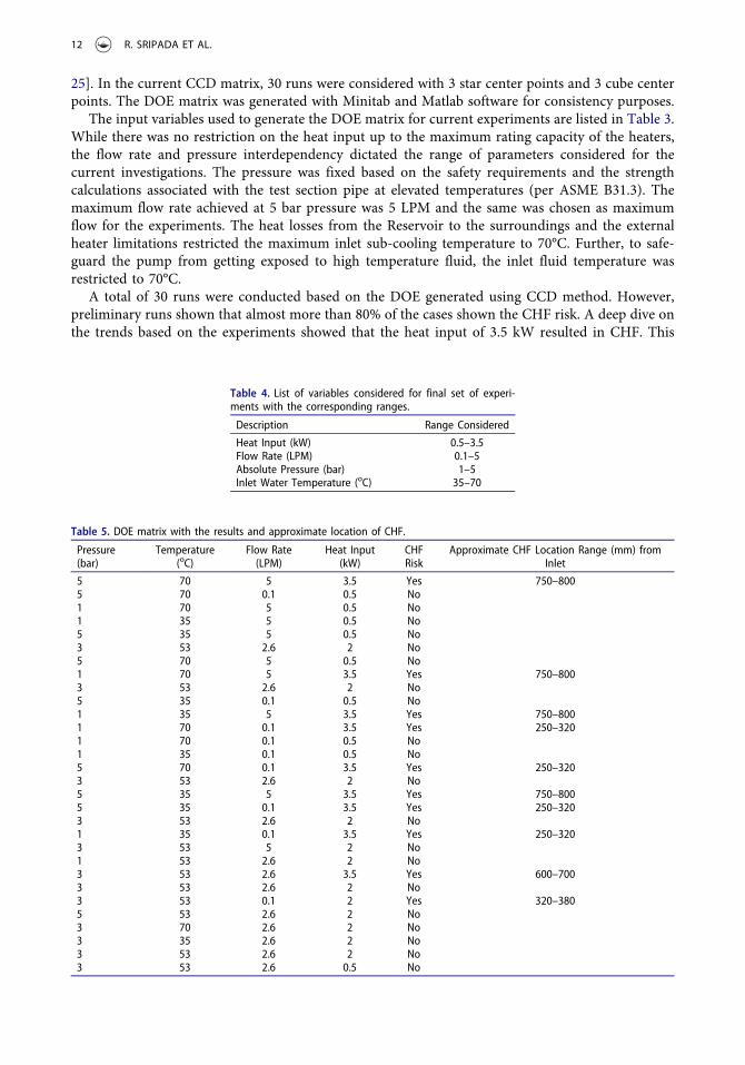
25]. In the current CCD matrix, 30 runs were considered with 3 star center points and 3 cube centerpoints. The DOE matrix was generated with Minitab and Matlab software for consistency purposes.

The input variables used to generate the DOE matrix for current experiments are listed in Table 3.While there was no restriction on the heat input up to the maximum rating capacity of the heaters,the flow rate and pressure interdependency dictated the range of parameters considered for thecurrent investigations. The pressure was fixed based on the safety requirements and the strengthcalculations associated with the test section pipe at elevated temperatures (per ASME B31.3). Themaximum flow rate achieved at 5 bar pressure was 5 LPM and the same was chosen as maximumflow for the experiments. The heat losses from the Reservoir to the surroundings and the externalheater limitations restricted the maximum inlet sub-cooling temperature to 70°C. Further, to safe-guard the pump from getting exposed to high temperature fluid, the inlet fluid temperature wasrestricted to 70°C.

A total of 30 runs were conducted based on the DOE generated using CCD method. However,preliminary runs shown that almost more than 80% of the cases shown the CHF risk. A deep dive onthe trends based on the experiments showed that the heat input of 3.5 kW resulted in CHF. This

Table 4. List of variables considered for final set of experi-ments with the corresponding ranges.

Description Range Considered

Heat Input (kW) 0.5–3.5Flow Rate (LPM) 0.1–5Absolute Pressure (bar) 1–5Inlet Water Temperature (oC) 35–70

Table 5. DOE matrix with the results and approximate location of CHF.

Pressure(bar)

Temperature(oC)

Flow Rate(LPM)

Heat Input(kW)

CHFRisk

Approximate CHF Location Range (mm) fromInlet

5 70 5 3.5 Yes 750–8005 70 0.1 0.5 No1 70 5 0.5 No1 35 5 0.5 No5 35 5 0.5 No3 53 2.6 2 No5 70 5 0.5 No1 70 5 3.5 Yes 750–8003 53 2.6 2 No5 35 0.1 0.5 No1 35 5 3.5 Yes 750–8001 70 0.1 3.5 Yes 250–3201 70 0.1 0.5 No1 35 0.1 0.5 No5 70 0.1 3.5 Yes 250–3203 53 2.6 2 No5 35 5 3.5 Yes 750–8005 35 0.1 3.5 Yes 250–3203 53 2.6 2 No1 35 0.1 3.5 Yes 250–3203 53 5 2 No1 53 2.6 2 No3 53 2.6 3.5 Yes 600–7003 53 2.6 2 No3 53 0.1 2 Yes 320–3805 53 2.6 2 No3 70 2.6 2 No3 35 2.6 2 No3 53 2.6 2 No3 53 2.6 0.5 No

12 R. SRIPADA ET AL.

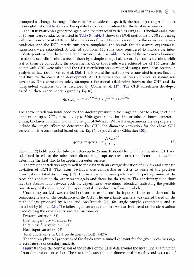
prompted to change the range of the variables considered, especially the heat input to get the moremeaningful data. Table 4 shows the updated variables considered for the final experiments.

The DOE matrix was generated again with the new set of variables using CCD method and a totalof 30 runs were conducted as listed in Table 5. Table 5 shows the DOE matrix for the 30 runs alongwith the occurrence of CHF and likely location of the CHF occurrence. Once the experiments wereconducted and the DOE matrix runs were completed, the bounds for the current experimentalframework were established. A total of additional 120 runs were considered to include the inter-mediate points within the bounds. These are not listed in Table 5. A few of the runs were eliminatedbased on visual elimination, a few of them by a simple energy balance or the hand calculation, whilerest of them by conducting the experiments. Once the results were achieved for all 150 cases, thepoints with CHF were taken and the CHF correlation was developed using a non-linear regressionanalysis as described in Sarma et al. [26]. The flow and the heat rate were translated to mass flux andheat flux for the correlation development. A CHF correlation that was empirical in nature wasdeveloped. This correlation solely attempts a functional relationship between the CHF and theindependent variables and as described by Collier et al. [27]. The CHF correlation developedbased on these experiments is given by Eq. (8).

qCHF;Dref ¼ 93 � P0:0629 � T�0:03867in � G0:07982 (8)

The above correlation holds good for the absolute pressure in the range of 1 bar to 5 bar, inlet fluidtemperature up to 70°C, mass flux up to 3000 kg/m2 s, and for circular tubes of inner diameter of6 mm, thickness of 1 mm, and with a length of 960 mm. While the experiments are in progress toinclude the length effects to determine the CHF, the diametric correction for the above CHFcorrelation is recommended based on the Eq. (9) as provided by Ghiaasian [20].

qCHF;D ¼ qCHF;Dref �Dref

D

� �0:5

(9)

Equation (9) holds good for tube diameters up to 25 mm. It should be noted that the above CHF wascalculated based on the tube inner diameter appropriate area correction factor to be used todetermine the heat flux to be applied on outer surface.

The present correlation agrees well to the data with an average deviation of 13.87% and standarddeviation of 18.71%. The mean deviation was comparable or better to some of the previousinvestigations listed by Chang [12]. Consistency runs were performed by picking some of thecases and conducting the experiments again and check for the results. The consistency runs showthat the observations between both the experiments were almost identical, indicating the possibleconsistency of the results and the experimental procedure itself on the whole.

Uncertainty analysis was carried both on the results and the input variables to understand theconfidence levels on the predictions of the CHF. The uncertainty analysis was carried based on themethodology proposed by Kline and McClintock [28] for single sample experiments and asdescribed by Moffat [29]. The following uncertainty numbers were arrived based on the observationsmade during the experiments and the instruments.

Pressure variation: 6%Inlet temperature variation: 9%Inlet mass flux variation: 12%Heat input variation: 9%Total uncertainty in CHF prediction (output): 9.42%The thermo-physical properties of the fluids were assumed constant for the given pressure range

to estimate the uncertainty analysis.Figure 8 shows the comparison of the scatter of the CHF data around the mean line as a function

of non-dimensional mass flux. The x-axis indicates the non-dimensional mass flux and is a ratio of

EXPERIMENTAL HEAT TRANSFER 13

the mass flux to the maximum mass flux used in current investigations. The y-axis indicates the ratioof CHF calculated by the correlation to the CHF values based on the experiments. The results wereshown for all the pressure cases, and for all the inlet fluid temperatures. As it is evident from Figure8, most of the data points were within the ±30% line. From the current investigations, it wasobserved that the estimated values were more scattered at low mass fluxes as compared to highmass fluxes, indicating the correlation predicted value to be different to the experimental value. Thiswas in line with some of the previous investigations where the CHF was dominant in verticallydownward two-phase flows at low mass flow rates and at low pressures. This could be attributed tothe dominance of two-phase flow instabilities as well at low flow rates. At high mass fluxes, moredata were distributed closer to the mean line indicating that the correlation predicted value and theexperimental value were almost the same.

Figure 9 shows the comparison of the correlation value to the experimental value at low mass fluxof 58.6 kg/m2 s, intermediate mass flux of 1400 kg/m2 s and high mass flux of 3000 kg/m2 s, forwater inlet temperature of 53°C, and at all pressures. Trends from Figure 9 clearly show that thedifference in estimated value from the correlation and the experimental value increases with thedecrease in pressure and at low flow rate. The same trend was not observed at average and high massfluxes, indicating the possible complex flow mechanism associated with low mass flow rate at low

Figure 8. Comparison of the calculated CHF value to the experimental value to the non-dimensional mass flux for all pressurecases.

Figure 9. Comparison of the calculated CHF value to the experimental value at low, intermediate and high mass fluxes, inlettemperature of 53°C and at all the pressures.

14 R. SRIPADA ET AL.

pressures as described by several previous investigators. Figure 10 shows the effect of mass flux onCHF for different pressures considered for current experiments. As expected, the CHF magnitudeenhances with increase in pressure. The enhancement of CHF is found to be ~10–12% for 5 barwhen compared to 1 bar pressure. The chart was shown for different Lcritical/D and critical quality.The purpose of this chart is to ensure that the trends from the correlation are in consistent with themeasurement.

Conclusions

An experimental test rig was designed, developed and successfully commissioned to investigate theCHF in two-phase flows directed vertically downwards. Safety was given top most priority during thedesign and commissioning of this test rig. A few additional design features were included in the testrig to enhance the CHF predictions. Some of them include uniform heating of the test section byincorporating six discrete cylindrical heaters with test section passing through the center of theheaters. Further, a provision to have variable heating length and non-uniform heating by switchingoff/on/regulating the power input to the heaters can be achieved without any modifications.

A CHF correlation was developed in a round tube for vertically downward two-phase flows withwater-steam mixtures as a function of variables including mass flux, inlet sub-cooled temperature ofliquid and the pressure up to 5 bar. The trends observed from the current investigations were in linewith some of the previous investigations at low mass fluxes and at atmospheric conditions. The CHFmeasured deviates significantly to as much as 3 to 4 times at high mass fluxes when compared toprevious investigations due to the absence of inlet throttling or plenum, thus constituting the CHFpredicted to be minimal and constitutes the lower bound.

The estimations from the developed correlation were in agreement with the present experimentalvalues at high and intermediate mass fluxes while deviate at low mass fluxes indicating the complex-ity associated with flow patterns at low mass fluxes. The developed correlation can predict the CHFwith a mean deviation of 13.87% and a standard deviation of 18.71% when compared with currentexperimental data. The uncertainty analysis revealed a 90% confidence level on the CHF estimatedue to variation in the input variables.

Current investigations also show significant two-phase flow instabilities at low pressures due tothe increased differences in the density between the gas and the liquid phases. The experiments alsorevealed reduced risk due to premature tube burnout at high pressures due to continuous wetting of

Figure 10. Qualitative trends from current investigations – Influence of mass flux on CHF at various pressures.

EXPERIMENTAL HEAT TRANSFER 15

wall with liquid films. This forms an important conclusion as most of the boilers in conventionalpower plants and chemical plants operate at very high pressures and mass fluxes.

The current experiments extended the previous investigators conclusion by including the pressureeffects up to 5 bar. The current studies could be further extended to include pressure effects above5 bar, by varying the inlet fluid temperatures and flow rates and come up with a more robust CHFcorrelation that could be used for broader range of parameters as it is available for vertically upwardflows and horizontal flows.

Acknowledgments

The authors would like to acknowledge the Management and the staff of Mechanical, Civil and Electrical departmentof MVGR College of Engineering, Vizianagaram, India for allowing to commission the test rig and providing necessaryinfrastructure including manpower, electricity and water that helped in conducting these experiments. Authors wouldalso like to thank the students Mohana Pabbisetty, Sai Sunkari Naidu and Srikanth Sahu for their valuable contribu-tions during conducting the experiments. Special thanks also go to Management of University of South Africa forproviding an opportunity to do this research from their esteemed organization.

Nomenclature

A: Cross sectional area (m2)AH: Heated area (m2)C: Constant as defined by Mishima [11]Co: Distribution parameterCp: Specific heat at constant pressure (J/kg-K)D: Diameter (m)D*: Dimensionless diameterDref: Reference diameter (8mm)F: Empirical correlation constant as defined by Sudo et al. [10]

G*: Dimensionless downward water mass fluxG: Mass flux (kg/m2s)g: Acceleration due to gravity (m/s2)

hlv: Latent heat of vaporization (J/kg)l: Length (m)

NPS: Nominal pipe sizeONB: Onset of nucleate boiling

P: Pressure (bar)q: Heat flux (kW/m2)

qCHF*: Dimensionless CHFqCL: Critical heat flux for low mass flux (kW/m2)qCF: Flooding limited CHF (kW/m2)qcH: Critical heat flux for high mass flux (kW/m2)qw”: Critical heat flux (kW/m2)

SCH: Schedule (for pipe)Tin: Inlet water temperature (oC)TSat: Saturation temperature (oC)Tsub: Inlet water subcooling (oC)TW: Wall temperature (oC)Vgj: Superficial gas velocity (m/s)

Greek Symbolsε: Void fractionχ: Qualityλ: Characteristic wave length (m) (= [σ/(γl- γg)]

1/2 for Eq. 3.)ρv, ρg: Vapor/gas density (kg/m3)

ρl: Liquid density (kg/m3)γ: Specific weight (kg/m3)σ: Surface tension (kg/m)

16 R. SRIPADA ET AL.

References

[1] S. M. Bhagwat, “Study of flow patterns and void fraction in vertical downward two-phase flow,” Master’sDissertation, Dept. of Mech. Engr., Oklahoma State University, Oklahama, 2011.

[2] D. Hall David and M. Issam, “Critical heat flux for water flow in Tubes-I. Compilation and assessment of worldCHF data,” Int. J. Heat Mass Transf., vol. 43, pp. 2573–2604, 2000. DOI: 10.1016/S0017-9310(99)00191-X.

[3] D. Hall David and M. Issam, “Critical heat flux for water flow in Tubes-II. Sub-cooled CHF correlations,” Int.J. Heat Mass Transf., vol. 43, pp. 2605–2640, 2000. DOI: 10.1016/S0017-9310(99)00192-1.

[4] S. Stephen Papell, R. J. Simoneau, and D. D. Brown., “Buoyancy effects on critical heat flux of forced convectiveboiling in vertical flow,” NASA TN D-3672, Lewis Research Center, Cleveland, Ohio, October 1966.

[5] A. R. Blumenkrantz and W. R. Gambill, “Buoyancy effects on thermal burnout with downflow of water invertical channels,” Nucl. Saf., vol. 9, pp. 467–480, 1968.

[6] M. Cumo, R. Bertoni, R. Cipriani, and G. Palazzi, “Upflow and downflow burnout,” Inst. Mech. Engrs. Conf.Publ., vol. 8, pp. 183–192, 1977.

[7] M. Kaichiro, N. Hiedeaki, and M. Itaru, “Boiling burnout and flow instabilities for water flowing in a roundtube under atmospheric pressure,” Int. J. Heat Mass Transf., vol. 28, pp. 1115–1129, 1985. DOI: 10.1016/0017-9310(85)90120-6.

[8] M. Kaichiro and N. Hiedeaki, “Effect of channel geometry on critical heat flux for low pressure water,” Int.J. Heat Mass Transf., vol. 30, pp. 1169–1182, 1987. DOI: 10.1016/0017-9310(87)90046-9.

[9] Y. Sudo, K. Miyata, H. Ikawa, M. Kaminaga, and M. Ohkawara, “Experimental study of differences in DNB heatflux between upflow and downflow in vertical rectangular channel,” J. Nucl. Sci. Technol., vol. 22, pp. 604–618,1985. DOI: 10.1080/18811248.1985.9735705.

[10] Y. Sudo and M. Kaminaga, “A CHF characteristic for downward flow in a narrow vertical rectangular channelheated from both sides,” Int. J. Multiphase Flow, vol. 15, pp. 755–766, 1989. DOI: 10.1016/0301-9322(89)90039-6.

[11] K. Mishima, “Boiling burnout at low flow rate and low pressure conditions,” Dissertation Thesis, KyotoUniversity, Japan, 1984.

[12] S. W. Ruan, G. Bartsch, and S. M. Yang, “Characteristics of the critical heat flux for downward flow in a verticaltube at low flow rate and low pressure conditions,” Exp. Therm. Fluid Sci., vol. 7, pp. 296–306, 1993. DOI:10.1016/0894-1777(93)90053-L.

[13] S. H. Chang, W. P. Baek, and T. M. Bae, “A study of critical heat flux for low low flow of water in vertical roundtubes under low pressure,” Nucl. Eng. Des., vol. 132, pp. 225–237, 1991. DOI: 10.1016/0029-5493(91)90267-L.

[14] A. Srivastava and G. K. Sinha, “Experiments to Compare the dynamics and thermal impact of single vaporbubble subjected to upward and downward flow boiling configurations,” Exp. Heat Transfer, 2019. DOI:10.1080/08916152.2019.1662518.

[15] K. Aroonrat, A. S. Dalkilic, and S. Wongwises, “Experimental study on evaporative heat transfer and pressuredrop of R-134a flowing downwards through vertical corrugated tubes with different corrugation pitches,” Exp.Heat Transfer, vol. 26, pp. 41–63, 2013. DOI: 10.1080/08916152.2011.631080.

[16] S. Zhi, D. Yang, G. Chen, and F. Xiao, “Experimental investigation on heat transfer characteristics of smoothtube with downward flow,” Int. J. Heat Mass Transf., vol. 68, pp. 669–676, 2014. DOI: 10.1016/j.ijheatmasstransfer.2013.09.045.

[17] H. A. Mohammed and Y. K. Salman, “Heat Transfer Measurements of Mixed Convection for Upward andDownward Laminar Flows Inside a Vertical Circular Cylinder,” Exp. Heat Transfer, vol. 21, pp. 1–23, 2008.DOI: 10.1080/08916150701647801.

[18] R. Sripada and V. R. Veeredhi, “Review of critical heat flux in a vertically downward two-phase flow.”Proceedings of the 24th National and 2nd International ISHMT-ASTFE Heat and Mass Transfer Conference(IHMTC-2017), Hyderabad, India, 2017. DOI: 10.1615/IHMTC-2017.2940.

[19] ASME B31.3, Process Piping Code. The American Society of Mechanical Engineers, New York, USA, 2016.[20] F. Mayinger, O. Schad, and E. Weiss, “Investigations into the critical heat flux in boiling water,” EURAEC

report No. 1811, Germany, 1967. http://Core.ac.uk/download/pdf/91636448.pdf.[21] P. Saha and N. Zuber, “Point of net vapor generation and vapor void fraction in subcooled boiling.”

Proceedings of the 5th International Heat Transfer Conference, Tokyo, Japan, 1974.[22] M. Ishii and T. Hibiki, Thermo-Fluid Dynamics of Two-Phase Flow. NewYork: Springer Publications, 2006.[23] S. M. Ghiaasiaan, Two-Phase Flow, Boiling, and Condensation in Conventional and Miniature Systems, 2nd ed.

Cambridge: Cambridge University Press, 2017.[24] J. Kiemele Mark, R. Schmidt Stephen, and J. Berdine Ronald, Basic Statistics - Tools for Continuous

Improvement, 4th ed. Colarado Springs: Air Academy Press, 1999.[25] B. Dodson, P. C. Hammett, and R. Klerx, Probabilistic Design for Optimization and Robustness for Engineers, 1st

ed. USA: John Wiley and Sons Ltd., 2014.[26] P. K. Sarma, et al., “An approach to predict convective turbulent heat transfer for non-newtonian fluid flow in a

tube,” Int. J. Heat Technol., vol. 24, pp. 133–141, 2006.

EXPERIMENTAL HEAT TRANSFER 17

[27] J. G. Collier and J. R. Thome, Convective Boiling and Condensation, 3rd ed. Oxford: Oxford SciencePublications, 1996.

[28] S. J. Kline and F. A. McClintock, “Describing uncertainties in single sample experiments,” Mech. Eng., vol. 3-8,pp. 3–9, 1953.

[29] R. J. Moffat, “Describing the uncertainties in experimental results,” Exp. Therm. Fluid Sci., vol. 1, pp. 3–17,1988. DOI: 10.1016/0894-1777(88)90043-X.

18 R. SRIPADA ET AL.

Proceedings of the 24th National and 2nd International ISHMT-ASTFE

Heat and Mass Transfer Conference (IHMTC-2017), December 27-30, 2017, BITS Pilani, Hyderabad, India.

IHMTC 2017-13-0522

REVIEW OF CRITICAL HEAT FLUX IN A VERTICALLY DOWNWARD TWO PHASE FLOW

Rajeshwar Sripada a,*, Veeredhi Vasudeva Rao b,

aUniversity of South Africa, Johannesburg, South Africa, rajeshwar33482@gmail.com bUniversity of South Africa, Johannesburg, South Africa, v_vasudevarao@yahoo.com

ABSTRACT Critical heat flux (CHF) or post burnout refers to the sudden decrease in heat transfer coefficient for a surface on which evaporation or boiling occurred. Exceeding this heat flux causes the replacement of liquid adjacent to the heat transfer surface with a vapor blanket. This blanket acts as a barrier to heat flow from the heat dissipating body, resulting in possible catastrophic failure. Two-phase flows were encountered in various applications including boilers and heat exchangers used in power plants, chemical plants and nuclear industry. The current day boiler industry application dictates for operation of boilers and heat exchangers over a wide range of operating conditions, starting from low pressure to very high pressure and high temperatures. The operation in harsh environment driven by high temperature corrosive gases prompts for usage of expensive materials and thermal coatings to protect from tube burnout and thereby improve the life. On the other hand, the efficiency of the heat exchanger strongly depends upon the surface area. The transportation limits put several constraints on making the heat exchanger fatter or taller, thereby adding to the complexity. To make these heat exchangers compact without compromising on its efficiency, one should look for alternative ways. One of the ways of doing it was to increase the number of passes by routing tubes in such a way that the two phase mixture travels downwards and upwards in a periodical manner. This brings in additional risks of premature tube burnout, 2 phase flow instabilities and other potential risks, especially in vertically downward flow. Accurate estimation of CHF risk was a mandate not only from performance or life perspective, but also more importantly from safety perspective.

NOMENCLATURE

A: Area (m2), Flow area (m2) Ah: Heated area of channel (m2) a: Channel width (m) Cp: Specific heat (J/kgK) Pr: Prandtl number Re: Reynolds number G: Mass flow rate (kg/s) G*: Dimensionless mass flow rate d: Diameter (m) g: Acceleration due to gravity (m/s2) q”: Heat flux (W/m2) P: Pressure l: Length (m) hfg: Latent heat of vaporization (J/kg) DNB: Departure from nucleate boiling CHF: Critical heat flux (W/m2) T: Temperature (C) Co: Distribution parameter D*: Dimensionless tube diameter qcF: Flooding CHF qcp: Pool-boiling CHF qcF*: Dimensionless CHF due to flooding qcL*: Dimensionless CHF in the Katto L-regime qcP*: Dimensionless pool-boiling CHF Eo: Eotvos number Bo: Bond number Fr: Froude number : Void fraction β: Volumetric fraction λ: Taylor wavelength scale x: Steam quality ρ: Density (kg/m3)

μ: Viscosity (kg/m-s) σ: Surface tension (N/m) g, G: Gas l, L: Liquid v: Vapor h: Homogeneous sub: Subcooling i: inner o: outer c-s: Cross sectional PREVIOUS CHF INVESTIGATIONS ON VERTICALLY DOWNWARD TWO PHASE FLOW Significant amount of work was done on two phase flows in last 50 years, primarily focusing on understanding the flow patterns, estimating the void fractions and determining the critical heat flux (CHF) limits from the safety perspective. Most of the investigations in this field were predominantly focused on understanding the fluid flow patterns and heat transfer in horizontal tubes, inclined tubes, and in vertical tubes with the flow directed upwards. However, there were only limited investigations carried on vertically downward two phase flow, where the flow was directed downwards and the buoyancy of the bubbles compete with the gravity of the liquid, resulting in the most complex two-phase flow behavior. Investigations on vertically downward two phase were focused primarily on understanding the flow pattern maps and in estimating the void fractions [1-15], only a few investigations focused on understanding the CHF for vertically downward two phase flows. To add to this, most of these investigations on CHF for vertically downward two phase flow were conducted either at atmospheric pressure or slightly above the atmospheric pressure, giving an opportunity to explore the CHF risks associated with high pressures.

The present study was motivated by the fact that the CHF information on vertically downward two phase flow was limited. Hall and Mudawar [16, 17] compiled and assessed the CHF data based on work done by many investigators over a period of time, focusing on vertical upward flow and horizontal flow. There was lack of such a large, reliable, CHF database for developing correlations to predict CHF in a vertically downward two phase flow, covering a wide range of process conditions. This paper briefly discusses the limited work carried out on CHF for vertically downward flow, available CHF correlations and the range of process conditions in which they were applicable.

The investigations on vertically downward two phase flow were started even before 1966 but did not get the same level of importance as that of vertically upward flow or horizontal flow.

Papell et. al. [18] conducted experiments in a 12.8mm ID X 305mm long resistance heated instrumented tube with liquid nitrogen as working fluid. The system pressure was varied from 3.45 bar- 16.55 bar absolute, inlet velocity from 0.15mps-3.35mps and inlet sub-cooling from -266C to -245C. They had conducted experiments for both up-flow and down-flow. Under certain conditions, they found that the CHF for the downward flow was significantly lower than that for upward flow. The CHF in downward flow was subjected to buoyancy forces when the test conditions produce

an annular-dispersed type of flow and was not so when slug or bubbly flow exists. They also observed that the buoyancy effects on CHF for downward flow increased as pressure and sub-cooling decreased and decreased as the velocity increased. At velocities less than 0.6mps, they observed the predominance of buoyancy force causing the bubbles to rise against the flow and accumulate at the inlet. The momentum dominated the buoyancy beyond certain velocities. The temperature excursions were observed at the inlet, outlet or at any other position in the tube, depending on an interaction of the system variables. Although they had done extensive work covering higher pressures, they did not develop any CHF correlation for vertically downward flow.

Blumenkrantz and Gambill [19] observed down-flow CHF several-fold lower than up-flow CHF at very low mass velocities of water. Down-flow CHF obtained by Cumo et al. [20] for Freon-12 was about 11% lower than up-flow CHF when subjected to same conditions.

Mishima [21] developed the CHF correlation for vertically downward two phase flow, which was referred by Sudo and Kaminaga in their investigations [22]. Sudo and Kaminaga developed a CHF correlation for air-water downward flow in a narrow vertical rectangular channel heated from both the sides. They had conducted experiments for the countercurrent flow scenario wherein the water travels downwards while the air travels upwards. The experiments were conducted at 1atm with an inlet sub-cooling range of 25-75C and inlet mass flux range of 2600 kg/m2s and in 2.25mm and 2.80mm gap flow channels, heated from both the sides. They had developed the CHF correlation given by Equation 1.

𝑞∗ = 𝐺∗ +.

.

𝐹 . (1)

Where F given by Equation 2

F = 1.3 . − 1.52.

(0.5 + 0.0015Bo . )G∗ ..

(2)

Bo was Bond number given by Equation 3

Bo =.

(3)

and G* given by Equation 4

G∗ =( )

(4)

They had also referred to the CHF correlation for downward flow given by Mishima given by Equation 5.

𝑞∗ = 𝐺∗ + 𝐶/

(5)

The term λ was calculated using Equation6.

𝜆 =( )

/

(6)

Their experiments revealed an important effect of aspect ratio of rectangular channel on counter current flow limitation (CCFL) characteristics, based on the assumption that the CHF for downward flow was intimately related to the CCFL. They found that the proposed CHF correlation for downward flow in vertical rectangular channels based on new CCFL correlation has shown a much better coincidence with the experimental results than the prediction based on existing flooding correlation, making clear the undetermined role of the aspect ratio of the rectangular channel. It was strongly implied, both analytically and experimentally, that the CHF for downward flow was minimum under the flooding condition in the case of large inlet water sub-cooling and for an inlet downward water mass flux larger than that under the flooding condition in the case of small inlet water sub-cooling. Their investigation led to development of CHF correlation but was at atmospheric pressure.

Mishima et al. [23] studied the CHF at low mass velocities, flow stagnation and flow reversal conditions by conducting experiments with water and at atmospheric conditions. The test section was a 6mm ID, 1mm thick 244mm stainless steel tube. The main emphasis was given to the effects of buoyancy (up-flow and down-flow), upstream compressibility and inlet valve throttling. Based on their investigations, they found that for a stiff system (with large inlet throttling), the buoyancy had no effect for downward two phase flow. In both up-flow and down-flow, CHF increased linearly as the mass velocity increased at very low mass velocities. The stable flow CHF at low mass velocities could be well correlated by conventional high quality correlations such as Katto correlation. In down-flow, the CHF was as much as 30% lower than up-flow at very low mass velocities due to the effect of the buoyancy. The CHF at intermediate exit qualities appeared to be significantly affected by the density wave oscillations. At higher mass velocities, the flow direction has minimal impact. The CHF at low flow rate and low pressure conditions were largely affected by various flow instabilities. They also observed that due to the buoyancy, the down-flow was less stable than up-flow. At lower heat flux, the basic mechanism of burnout was observed due to dry-out or breakdown of the liquid film on heated surface, which was caused by the deficiency of the liquid in the heated section and might be controlled by hydro-dynamical phenomena as flooding or flow reversal, entrainment and deposition of liquid droplets. Further, flow instabilities like the density-wave oscillations, the pressure drop oscillations and the flow excursion could reduce the effective film flow rate, thus leading to premature burnout of the tube. When both the mass velocity and the heat flux were high, and the exit quality was near zero, the flow excursion appears to be the dominant phenomenon to cause the burnout. When the heat flux was sufficiently high, say, higher than the pool boiling CHF, a temporary reduction of flow rate due to flow instability initiated vapor-blanketing, which could not be quenched by the subsequent increase of the flow rate and results in departure from nucleate boiling (DNB)-type burnout.

Mishima et al. [24] further investigated the effect of channel geometry on CHF for low pressure water and for both up-flow and down-flow conditions. They had conducted experiments in annulus, rectangular ducts and round channels. For down-flows in rectangular channels, they found that the burnout occurred due to flooding at low mass velocities, less

than the critical value, to stagnate steam bubbles in the heated channel. Resultant CHF was at minimum. The critical mass velocity for bubble stagnation was calculated based upon the drift flux model given by Ishii given in Equation 7.

𝐺 = 2(𝜌 𝜎𝑔∆𝜌) / /𝐶 (7) The distribution parameter (C0) given by Equation 8 for annuli & round tubes, and for rectangular ducts. For annuli and round tubes

𝐶 = 1.2 − 0.2𝜌

𝜌

For rectangular ducts,

. 𝐶 = 1.35 − 0.35 (8)

For rectangular channels, at intermediate mass velocities beyond the critical mass velocity, they found that the burnout occurred at zero exit quality. In this region, vigorous flow oscillations arise, whose amplitude increased with increased mass velocity and heat flux. For round tubes, they found that for the stiff system, the CHF was as much as 30% lower than the up-flow high quality CHF at very low flow rates. However, the difference disappeared as the flow rate increased. At intermediate mass velocities, there was a region where the CHF was almost constant as a function of mass velocity, as was the case in up-flow. The CHF was lower as the flow becomes less stable. At sufficiently high mass velocities, burnout occurred due to flow excursion. These investigations were carried at pressure close to atmospheric pressure and there was no correlation developed.

Sudo et al. [25] studied the differences in departure for nucleate boiling (DNB) heat flux between up-flow and down-flow in a vertical rectangular channel. They had conducted experiments at a pressure of 0.981 – 1.18 bar, mass flux of 0-600 kg/m2s, inlet temperature range of 19-80C, tube diameters of 2.28mm and length to diameter ratio of 170.85. Based on their investigations, they found that the q" for down-flow was almost same as that of up-flow at very low G* including zero and at high G* larger than 300. At intermediate G* values of 1.5 to 200, q" for down-flow was much lower than the up-flow. Another interesting observation by them was that the inlet sub cooling of water was a key parameter for the down-flow at low G*, giving remarkably lower DNB heat flux with lower inlet sub-cooling of water. The non-dimensional G* was given by Equation 9. These investigations primarily focused on understanding DNB and at pressures close to atmosphere.

G∗ =( )

(9)

Chang et al. [26] studied the CHF risk for very low

flow of water in vertical round tubes under low pressure conditions. They had conducted experiments for both up-flow and down-flow scenarios and varying the inlet conditions like mass flux, sub-cooling and throttling. The experiments for down-flow were conducted covering a range of inlet temperatures of 20-70C, tube IDs of 6mm and 8mm, mass flux of 6-187 kg/m2s and using a stainless steel tube.

They had drawn a few conclusions based on their work. They found that the CHF monotonously increases as mass flux increases from zero regardless of the flow direction and inlet throttling for stable condition. When large inlet throttling was provided, the down-flow CHF was generally lower than the up-flow CHF but the difference was not that significant. On the other hand, they found it almost impossible to maintain a stable downward flow condition without inlet throttling indicating that the downward flow was much more susceptible to the instabilities and premature CHF due to flow excursion if they were not suppressed. The effect of inlet sub cooling was small and obscure in the stable low flow conditions under low pressure. Throttling just before the inlet of a boiling channel under low pressure increases the stability of flow, and therefore generally increases the CHF and was very important for down-flow conditions. The large diameter tube gives a higher CHF and a lower critical quality as expected.

They had developed the CHF correlation and the same was given by Equations 10 and 11 for low G* and high G* respectively.

q∗ = q∗ + 0.01351(D∗) . ( ) . |G∗| . (10)

q∗ = q∗ + 0.05664(D∗) . ( ) . |G∗| . (11)

The term q*cF given by Equation 12

q∗ = 1.61( ) 1 + ( ) / √D∗ (12)

The smaller of qcH and qcL would be taken as the CHF value.

Ruan, Bartsch, and Yang [27] studied the characteristics of CHF for downward flow in a vertical tube at low flow rates (0-200 kg/m2s) and pressure conditions (1 – 7 bar). They had used Inconel 600 circular tubes of 9mm inner diameter as test section in a water test loop. The attention was given to the effects of upstream conditions – upper plenum and inlet throttling. Although the investigations were carried at relatively high pressure, their work did not focus upon correlation development, but gave some good insights of typical CHF patterns observed due to variations in the upstream conditions.

They had observed two different kinds of CHF behavior for the case with larger upper plenum. The first behavior was characterized by the periodic wall temperature pulsation with greater amplitude for longer periods (10-20 s) along the entire test section, with vapor reaching the upper end of the test section. This was termed as CHF1 (flooding type) and was related to the sustained flow instability of the alternate occurrence of the co-current downward flow and counter-current flow in the bubbly or slug flow, caused by the combined effect of the upstream compressibility and buoyancy acting on the bubbles opposed to the flow direction. If the inlet sub-cooling was low and the water in the upper plenum was nearly saturated, this unstable boiling crisis could overcome with a further increase of heating power. Subsequently, they found that the down-flow boiling reached a new stable period until the wall temperature at the exit of the test section rose abruptly like the temperature excursion of an ordinary CHF at much higher heat flux. They termed this type of behavior as

CHF2, which was observed at high heat fluxes and could be interpreted as dry-out in annular flow. They did not observe CHF1 for the test sections without upper plenums.

For the stiff systems (with large inlet valve throttling), they observed a stable down-flow boiling regime. The wall temperature fluctuations were not observed and the location of CHF onset was at the exit of the test section, just the same as that of stable up-flow. For very low mass flow rates (less than 25 kg/m2s), the countercurrent flow occurred with the vapor reaching the upper end of the test section so that the inlet sub-cooling reduced considerably, but the CHF behavior remained unchanged. In a soft system – throttling at specific location, the CHF behavior was nearly the same as in the case of the stiff system, especially for very low mass velocity. For high mass fluxes, they observed that the onset was not strictly limited at the exit of the test section, and the CHF value was also somewhat lower than the stable CHF for same parameters. The difference became considerable when the throttling position moved to the location before the pre-heater. For high mass flux and at atmospheric pressure, wall temperature fluctuated before CHF occurred. The CHF region was about one third of the tube from the exit of the test section, and the CHF value was only about 40% of the stable CHF in the stiff system.

In addition, they had also investigated other parameters that would impact CHF1 and CHF2. They found that the CHF1 was nearly independent of mass flux, increases slightly with increase in degree of sub-cooling and was little by pressure, while CHF2 increases both with mass flux and degree of sub-cooling, and was independent of the pressure.

They had also compared the CHF1 data with the correlation proposed by Mishima et al. and found that their data was in good agreement. They had compared the CHF2 with the correlation of Weber and Weber & Johanssen for the stable up-flow CHF. They found the data to be in good agreement and concluded that it was reasonable to propose these two correlations as the lower and upper limits for the CHF for downward flow in vertical tube at low flow rate and low pressure conditions. Shen et al [28] conducted experiments to understand the heat transfer characteristics (HTC) of water in a smooth tube with downward flow. They had conducted experiments in the pressure range from 115 -280 bar, mass flux rates from 450 - 1550 kg/m2s and heat flux on inner wall from 50 - 585 kW/m2. Although they did not work on developing critical heat flux correlation, they had analyzed the effect of heat flux on heat transfer coefficient and wall temperature and the corresponding empirical correlations were presented accordingly. They had also compared their experimental results on heat transfer coefficients of downward flow with that of vertical upward flow and found that at subcritical and near critical pressure levels, the heat transfer performances was almost the same. However, when heat transfer deterioration occurred at these pressures, the temperature rise of walls in a vertical upward flow tube was higher than that of vertical downward flow tube. In addition, they had also found that at sub critical and at near critical pressure, dry out and departure from nucleate boiling could occur in vertical downward tube. With the increase of heat flux, heat transfer deterioration occurred ahead and the peak wall temperature after heat transfer deterioration increases. At supercritical pressure, the wall temperature increased slowly with fluid

enthalpy when the bulk temperature was lower than the pseudo-critical temperature and increased considerably when the bulk temperature was higher than the pseudo-critical temperature. SUMMARY Attempts were made earlier to understand the CHF patterns for a vertically downward two phase flow. As expected, most of the investigators found that the CHF for a vertically downward flow was lower than vertically upward flow at low mass fluxes and intermediate mass fluxes. At higher mass fluxes, the CHF limits were comparable for vertically upward and vertically downward flows. A few CHF correlations were proposed by a few authors but the development was based on limited number of experiments at relatively low pressures close to atmospheric pressure. Some of the authors investigated the heat transfer characteristics for a vertically downward flow and compared the same with vertically upward flow at close to critical pressures. Like the existence of a proper CHF database for vertically upward flow and horizontal flow, there was hardly any database existing for a vertically downward flow. Existing CHF correlations applicability for vertically downward flow should be investigated for a wider range of process conditions. All these limitations would give an opportunity to focus on the CHF aspects for a vertically downward flow and develop a database for CHF correlations, covering a wide range of process conditions. KEYWORDS: Heat Transfer, Critical Heat Flux, Fluid Properties, Vertically Downward Flow, Vertically Upward Flow, High Pressure REFERENCES:

1. Oshinowo. O, 1971. “Two Phase Flow in a Vertical Tube Coil.” PhD Thesis, Department of Chemical Engineering and Applied Chemistry, University of Toronto, Toronto. Cross referred via reference 12.

2. Yasaburo Yamazaki, and Katsuji Yamaguchi, 1979. “Characteristics of Cocurrent Two-Phase Down-flow in Tubes.” Journal of Nuclear Science and Technology, 16, pp. 245-255.

3. Golan. L, 1968. “An Air-Water Study of Vertical Upward and Downward Two Phase Flow.” PhD Thesis, Department of Mechanical Engineering, Leigh University, Leigh. Cross referred via reference 12.

4. Troniewski. L, Spisak. W, 1987. “Flow Patterns in Two-Phase Down-flow of Gas and Very Viscous Liquid.” International Journal of Multiphase Flow, 13, pp. 257-260.

5. Abdullah Abbas Kendoush, and Salah A. W. Al-Khatab, 1994. “Experiments on Flow Characterization in Vertical Downward Two-Phase Flow.” Experimental Thermal and Fluid Science 9, pp. 34-38.

6. Kensuke Usui, and Kazuo Sato, 1989. “Vertically Downward Two-Phase Flow, (I).” Journal of Nuclear Science and Technology, 26, pp. 670-680.

7. Kensuke Usui, and Kazuo Sato, 1989. “Vertically Downward Two-Phase Flow (II).” Journal of Nuclear Science and Technology, 26, pp. 1013-1022.

8. Yijun Jiang, and Kamiel S. Rezkallah, 1993. “A Study on Void Fraction in Vertical Co-Current Upward and Downward Two-Phase Gas-Liquid Flow (Part I: Experimental Results).” Chemical Engineering Communications, 126, pp. 221-243.

9. Yijun Jiang, and Kamiel S. Rezkallah, 1993. “A Study on Void Fraction in Vertical Co-Current Upward and Downward Two-Phase Gas-Liquid Flow (Part I: Experimental Results).” Chemical Engineering Communications, 126, pp. 245-259.

10. Crawford T. J., Weinberger C. B., and Weisman J, 1986, “Two-Phase Flow Patterns and Void Fraction in Downward Flow (Part I: Steady State Flow Patterns).” International Journal of Multiphase Flow, 11, pp. 761-782.

11. Crawford T. J., Weinberger C. B., and Weisman J, 1986, “Two-Phase Flow Patterns and Void Fraction in Downward Flow (Part I: Transient Flow Patterns).” International Journal of Multiphase Flow, 12, pp. 219-236.

12. Swanand Madhav Bhagwat, 2011. “Study of Flow Patterns and Void Fraction in Vertical Downward Two Phase Flow.” MS Thesis, Department of Mechanical Engineering, Oklahoma State University, Oklahama.

13. Melkamu A. Woldesemayat, Afshin J Ghajar, 2007. “Comparison of Void Fraction Correlations for Different Flow Patterns in Horizontal and Upward Inclined Pipes.” International Journal of Multiphase Flow, 33, pp. 347-370.

14. Butterworth D, 1975. “A Comparison of Some Void-Fraction Relationships for Co-Current Gas-Liquid Flow.” International Journal of Multiphase Flow, 1, pp. 845-850.

15. Takashi Hibiki, Hiroshi Goda, Seungjin Kim, Mamoru washii, Jennifer Uhle, 2004. “Structure of Vertical Downward Bubbly Flow.” International Journal of Heat and Mass Transfer, 47, pp. 1847-1862.

16. Hall David D., Mudawar Wassam, 2000. “Critical Heat Flux for Water Flow in Tubes-I. Compilation and Assessment of World CHF Data.” International Journal of Heat and Mass Transfer, 43, pp. 2573-2604.

17. Hall David D., Mudawar Wassam, 2000. “Critical Heat Flux for Water Flow in Tubes-II. Sub-Cooled CHF Correlations.” International Journal of Heat and Mass Transfer, 43, pp. 2605-2640.

18. Stephen Papell S, Robert J. Simoneau, Dwight D Brown, 1966. “Buoyancy Effects on Critical Heat Flux of Forced Convective Boiling in Vertical Flow.” NASA TN D-3672, Lewis Research Center, Cleveland, Ohio.

19. Blumenkrantz A. R., Gambill W. R., 1968. Buoyancy effects on thermal burnout with down-flow of water in vertical channels.” Nuclear Safety 9, pp. 467-480. Cross referred via reference 28.

20. Cumo M., Bertoni R., Cipriani R., Palazzi G., 1977. “Up-flow and down-flow burnout.” Inst. Mech. Engrs

Conference Publications, pp. 183-192. Cross referred via reference 28.

21. Mishima K., 1984. Boiling burnout at low flow rate and low pressure conditions, Dissertation Thesis, Kyoto University. Cross reference via Sudo and Kaminaga [5]

22. Sudo Y., Miyata K., Ikawa H., Kaminaga M., Ohkawara M., 1985. “Experimental Study of Differences in DNB Heat Flux between Up-flow and Down-flow in Vertical Rectangular Channel.” Journal of Nuclear Science and Technology, 22, pp. 604-618.

23. Mishima Kaichiro, Nishihara Hiedeaki, Michiyoshi Itaru, 1985. “Boiling Burnout and Flow Instabilities for Water Flowing in a Round Tube under Atmospheric Pressure.” International Journal of Heat and Mass Transfer, 28, pp. 1115-1129.

24. Mishima Kaichiro, Nishihara Hiedeaki, 1987. “Effect of Channel Geometry on Critical Heat Flux for Low Pressure Water.” International Journal of Heat and Mass Transfer, 30, pp. 1169-1182.

25. Sudo Y., Kaminaga M., 1989. “A CHF Characteristic for Downward Flow in a Narrow Vertical Rectangular Channel Heated from Both Sides.” International Journal of Multiphase Flow, 15, pp. 755-766.

26. Soon Heung Chang, Won Pil Baek, Tae Min Bae, 1991. “A Study of Critical Heat Flux for Low Low Flow of Water in Vertical Round Tubes under Low Pressure.” Nuclear Engineering and Design, 132, pp. 225-237.

27. Ruan S W., Bartsch G., Yang S M., 1993. “Characteristics of the Critical Heat Flux for Downward Flow in a Vertical Tube at Low Flow Rate and Low Pressure Conditions.” Experimental Thermal Fluid Science, 7, pp. 296-306.

28. Shen Zhi, Dong Yang, Gongming Chen, Feng Xiao, (2014). “Experimental Investigation on Heat Transfer Characteristics of Smooth Tube with Downward Flow.” International Journal of Heat and Mass Transfer, 68, pp. 669-676.

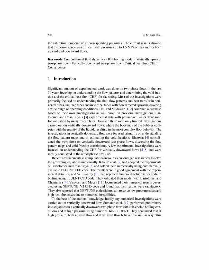
DEVELOPMENT OF CRITICAL HEAT FLUX CORRELATION IN CIRCULAR PIPE SECTIONS WITH VERTICALLY DOWNWARD TWO-PHASE FLOWS BY NUMERICAL ANALYSIS AND

COMPARISON WITH EXPERIMENTAL CORRELATION

Rajeshwar Sripada1, Vasudeva Rao Veeredhi Department of Mechanical and Industrial Engineering, University of South Africa,

Johannesburg, South Africa

Siva Subrahmanyam Mendu Department of Mechanical Engineering, Maharaj

Vijayaram Gajapathi Raj College of Engineering (A), Vizianagaram, India

ABSTRACT

Critical heat flux (CHF) and premature tube burnout are the common failure modes observed in steam water two-phase flows. Unlike the vertically upward two-phase flows, the vertically downward two-phase flows pose significant challenges including two-phase flow instabilities and premature tube burnout arising due to competing behavior between the buoyancy effects on vapor bubble and momentum and gravitational force acting on the liquid. Experimental investigations were conducted previously to understand the CHF at atmospheric pressures. There were very limited number of numerical analysis conducted in vertically downward flows using commercially available software and at such low-pressure conditions. In the current investigations, numerical simulations were carried with commercially available computational fluid dynamics software Fluent for vertically downward two-phase flows up to pressures of 5 bar. The magnitude of CHF from numerical investigations was compared with the experimental results conducted in house up to 5 bar and including the sub-cooling effects. The numerical results tend to agree with the experimental data at lower flow rates and at all pressures considered, but tend to deviate significantly at higher flow rates and at all pressures. Finally, A CHF correlation is proposed as a function of mass flux, inlet temperature and pressure. The proposed CHF correlations fits in with an average deviation of 16% and a standard deviation of 21%.

Keywords: Vertically downward two-phase flow, Critical Heat Flux, Computational Fluid Dynamics

1 Contact author: rajeshwar33482@gmail.com

NOMENCLATURE

Bf : Body force𝐹 : Interphase momentum force h: Specific enthalpy ��: Mass flow rate p: Pressure q: Heat flux Sq: External mass source SH.q: External heat source S∅,q: General turbulence model source termT: Temperature t: time �� : Velocity vector

Greek Symbols

α: Phase volume fraction ρ: Density ∅: General scalar Γ: Diffusion coefficient τq: Shear stress

Subscript and Superscript

c: Continuous D: Drag d: Dispersed in: Inlet l: Liquid

Proceedings of the ASME 2020 International Mechanical Engineering Congress and Exposition

IMECE2020 November 16-19, 2020, Virtual, Online

IMECE2020-23850

1 Copyright © 2020 ASME

q: qth phase r: rth phase TD: Turbulent dispersed v: Vapor w: Wall sub: Sub-cooling

1. INTRODUCTION

Critical heat flux (CHF) and premature tube burnout are the common failure modes observed in the multiphase flows, especially in steam water two-phase flows, frequently observed in heat exchangers and boilers used in nuclear, chemical and power industry. Lot of experimental investigations were conducted on CHF previously, giving importance to process conditions, fluids used, the geometry and the pipe orientation in which the fluids flow [1, 2]. Very limited number of experimental investigations were carried out in flows where the boiling two-phase fluid was directed in vertically downward direction. The complex two-phase flow associated with the competing nature of gravity, momentum and buoyancy acting in opposite directions leads to instabilities and premature tube burnout in vertically downward two-phase flows, thus making it challenging and interesting. Further, the ratio of liquid to gas density becomes larger and larger at lower pressures, thus constituting the worst scenario. This prompted most of the investigators to focus their research at these lower pressure conditions for vertically downward two-phase flows. Inlet throttling and other similar CHF enhancing mechanisms were also included in the previous investigations to suppress the possible two-phase flow instabilities and the premature tube burn out scenarios [3-6].

While experimental investigations are deemed to be ultimate to investigate the two-phase flows, numerical simulations are also getting due attention to mimic complex two-phase flows. Advancements in computational resources and availability of experimental data made a significant contribution to the development of boiling models in commercially available software. Validated numerical models paved way to do extensive simulations to understand the flow patterns inside the tubes for various operating scenarios, determining the location of CHF and optimize the design by mitigating the possible risks. Numerical simulations also assisted to reduce the number of experiments by screening the number of tests and allowing to conduct experiments on final few cases.

Huiying Li et al. [7] developed a numerical model to predict the boiling and CHF using a Eulerian model to account for boiling. They had developed the models in conjunction with the wall boiling models (RPI boiling model in Fluent) for nucleate modeling. The CHF and the non-equilibrium wall functions were modeled by extending the Rensselaer Polytechnic Institute (RPI) model to departure from nucleate boiling (DNB) by splitting the wall heat flux to both the liquid and vapor phases. They had validated the models with the experimental data for

vertically upward flows at high pressures and found the results to be in accord with the experimental data. Apart from developing the models and validating, importance was also given to the grid sensitivity investigations, turbulence models and other critical parameters in their investigations.

Ribeiro et al. [8] had conducted analysis of sub-cooled flow boiling in a vertically upward two-phase flow subjected to high pressure (45 bar) using CFD and at high mass fluxes. The numerical results were validated with the experimental data reported by Bartolomei et al. [9] for vertically upward flows, with emphasis given on the metal (wall) temperature, bulk fluid temperature of the liquid and the location of the DNB. The results showed that the numerical results were in accord with the plant data for the parameters listed above. Grid independent studies were also conducted and found that the results were less impacted with the grid except for the difficulties associated with the convergence.

Naveen et al. [10] had reported numerical solutions for sodium boiling using Fluent CFD code. They validated their numerical models with Bartolomei et al. for pressurized water simulations and refrigerant R12 with DEBORA experiments. Both these investigations were carried out at 45bar and 30.06 bar respectively. The results based on their numerical investigations were comparable with the experimental data.

Vyskocil et al. [11] documented their numerical results generated using NEPTUNE_V2 CFD and Fluent CFD codes with refrigerant R12 at high pressure in vertically upward two-phase flows and validated with the numerical experiments by Debora for vertically upward flows. They concluded that both the model results were comparable and were in good agreement with the experimental data.

Sumanth et al. [12] performed numerical simulations using Fluent CFD code for vertically downward flows. They had validated the existing models to predict void fraction, wall temperature and CHF in upward flows with the experimental data available publicly and extended the validated models to simulate vertically downward flows at high pressures and high mass fluxes. They concluded that at high pressures and high mass fluxes, the numerical simulations show hardly any difference between upward flow and downward flow indicating the minimal impact of flow direction at these conditions. Like the other investigators, even they concluded that the grid dependency checks did not show significant impact on the overall results.

It is evident from the above discussion that numerical analyses were carried out to understand the boiling phenomenon inside the tubes with flow directed vertically upwards. Most of these simulations were conducted at high pressure and with high mass fluxes and by including sub-cooling effects. Different types of fluids were considered for the simulations. All these simulations were validated with the experimental results

2 Copyright © 2020 ASME

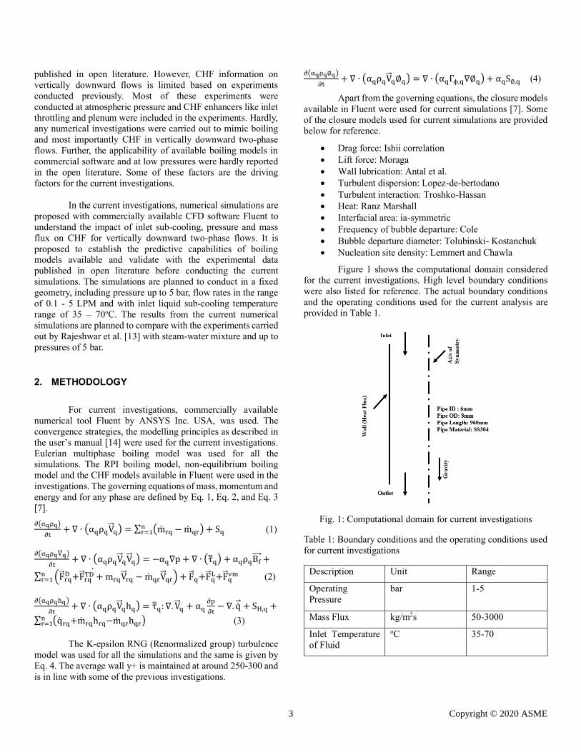
published in open literature. However, CHF information on vertically downward flows is limited based on experiments conducted previously. Most of these experiments were conducted at atmospheric pressure and CHF enhancers like inlet throttling and plenum were included in the experiments. Hardly, any numerical investigations were carried out to mimic boiling and most importantly CHF in vertically downward two-phase flows. Further, the applicability of available boiling models in commercial software and at low pressures were hardly reported in the open literature. Some of these factors are the driving factors for the current investigations.

In the current investigations, numerical simulations are proposed with commercially available CFD software Fluent to understand the impact of inlet sub-cooling, pressure and mass flux on CHF for vertically downward two-phase flows. It is proposed to establish the predictive capabilities of boiling models available and validate with the experimental data published in open literature before conducting the current simulations. The simulations are planned to conduct in a fixed geometry, including pressure up to 5 bar, flow rates in the range of 0.1 - 5 LPM and with inlet liquid sub-cooling temperature range of 35 – 70oC. The results from the current numerical simulations are planned to compare with the experiments carried out by Rajeshwar et al. [13] with steam-water mixture and up to pressures of 5 bar.

2. METHODOLOGY

For current investigations, commercially available numerical tool Fluent by ANSYS Inc. USA, was used. The convergence strategies, the modelling principles as described in the user’s manual [14] were used for the current investigations. Eulerian multiphase boiling model was used for all the simulations. The RPI boiling model, non-equilibrium boiling model and the CHF models available in Fluent were used in the investigations. The governing equations of mass, momentum and energy and for any phase are defined by Eq. 1, Eq. 2, and Eq. 3 [7]. ∂(αqρq)

∂t+ ∇ ∙ (αqρqV q) = ∑ (mrq − mqr)

nr=1 + Sq (1)

∂(αqρqV q)

∂t+ ∇ ∙ (αqρqV qV q) = −αq∇p + ∇ ∙ (τq) + αqρqBf

+

∑ (F rqD +F rq

TD + m

rqV rq − mqrV qr)nr=1 + F q+F q

L+F qvm (2)

∂(αqρqhq)

∂t+ ∇ ∙ (αqρqV qhq) = τq: ∇. V q + αq

∂p

∂t− ∇. q + SH,q +

∑ (qrq+mrqhrq−mqrhqr)nr=1 (3)

The K-epsilon RNG (Renormalized group) turbulence model was used for all the simulations and the same is given by Eq. 4. The average wall y+ is maintained at around 250-300 and is in line with some of the previous investigations.

∂(αqρq∅q)

∂t+ ∇ ∙ (αqρqV q∅q) = ∇ ∙ (αqΓϕ,q∇∅q) + αqS∅,q (4)

Apart from the governing equations, the closure models available in Fluent were used for current simulations [7]. Some of the closure models used for current simulations are provided below for reference.

• Drag force: Ishii correlation• Lift force: Moraga• Wall lubrication: Antal et al.• Turbulent dispersion: Lopez-de-bertodano• Turbulent interaction: Troshko-Hassan• Heat: Ranz Marshall• Interfacial area: ia-symmetric• Frequency of bubble departure: Cole• Bubble departure diameter: Tolubinski- Kostanchuk• Nucleation site density: Lemmert and Chawla

Figure 1 shows the computational domain consideredfor the current investigations. High level boundary conditions were also listed for reference. The actual boundary conditions and the operating conditions used for the current analysis are provided in Table 1.

Fig. 1: Computational domain for current investigations

Table 1: Boundary conditions and the operating conditions used for current investigations

Description Unit Range

Operating Pressure

bar 1-5

Mass Flux kg/m2s 50-3000

Inlet Temperature of Fluid

oC 35-70

3 Copyright © 2020 ASME

Apart from the models discussed above, the following high-level assumptions were made for these investigations:

• The properties were generated from steam tables forboth the liquid and vapor phase.

• 2d axi-symmetric model was used• Metal thickness was not modelled• Impurities in the water were not considered• Fully developed flow at the inlet

Ansys Fluent version 19 was used for the current investigations. The next section discusses the details related to the current numerical investigations.

3. RESULTS AND DISCUSSION

This section discusses about some of the key results obtained from the current investigations. Before conducting the investigations with the boundary conditions provided in Table 1, the models were validated. Since there were hardly any simulations carried out explicitly with vertically downward two-phase flows, model validation was done with vertically upward two-phase flows. Validated models were then extended to the vertically downward two-phase flows. Grid independent studies were conducted and found that the impact was negligible and is in line with previous investigations [7, 12]. Figure 2 shows the validation of the vertically upward two-phase flow CHF prediction from numerical analysis with the experimental data [9]. The graph also shows the extension of validated vertically upward flow model to the vertically downward flow [12].

Fig. 2: Validation of the numerical models for CHF with experimental data [9] and extension to downward flow, plot

from work by Sumanth et al. [12].

The validation work was done as part of earlier investigations and the results were validated at high pressures. As it is evident from Fig. 2, the upward flow CFD model was comparable with

the experimental data. The extension of validated CFD model for vertically downward flow shown almost a mirror image indicating that the flow direction has minimal impact at high mass fluxes and is in line with some of the previous conclusions [3, 4, 5]. The same models finalized for the validation were used in current investigations. The simulations were conducted for different combinations of flow rates, pressures and inlet fluid temperatures as listed in Table 1. The average y+ value was maintained around 250-300 for all the simulations and was in line with some of the previous investigations [7, 14].

The trends from the current simulations were validated with the experiments conducted by Rajeshwar et al. [13]. They designed and developed a sophisticated experimental test rig that was commissioned to conduct two-phase steam water flow experiments with flow directed vertically downwards in a round tube. The experimental test rig was specifically designed to conduct experiments up to 5 bar pressure and mass fluxes up to 3000 kg/m2s. The inlet sub-cooling was considered while conducting their experiments. Critical heat flux enhancers like inlet throttling and inlet plenum were not considered. They developed an experimental CHF correlation as a function of inlet mass flux, inlet pressure and inlet liquid temperature in the absence of CHF enhancers. The data from the current investigations was compared with the experimental data/ CHF correlation developed by Rajeshwar et al. [13]. Figure 3 shows the comparison of the critical heat flux values from current numerical simulations with the experimental data/ correlation at different pressures, at low mass flux of 50 kg/m2s and at inlet fluid temperature of 35oC.

Fig. 3: Comparison of the numerical models for CHF with experimental data from Rajeshwar et al. [13] at 50 kg/m2s and

inlet temperature of 35oC.

As it is evident from Fig. 3, the results from current CFD matches well with the experimental data at low mass flux of 50 kg/m2s. The CHF from CFD simulations was considered when there was an abrupt rise in metal temperature. Figure 4 shows the maximum metal temperature monitor point on the wall of the tube. The result is shown for the low flow rate case of 50 kg/m2s and at atmospheric pressure, where CHF was observed. There was an abrupt rise in temperature exceeding the safe limit 673K (400oC) beyond which the metal mechanical properties change

4 Copyright © 2020 ASME

abruptly [13]. Figure 5 shows the volume fraction at the exit for the same low mass flux case.

Fig. 4: Maximum metal temperature on the tube wall from CFD analysis for low mass flux [50 kg/m2s] case and at atmospheric

pressure.

As it is evident from Fig. 5, the numerical simulations shown significant amount of vapor at the exit. The same trend was observed from the previous experimental investigation. The experimental investigations of Rajeshwar et al. [13] also shown a periodic flow of water droplets indicating significant phase to be vapor. Thus, the CFD predictions show comparable trends with the experimental data at low flow rate of 50 kg/m2s.

Fig. 5: Average volume fraction of Vapor at Exit from CFD analysis for low mass flux [50 kg/m2s] and at atmospheric pressure condition.

Figure 6 shows the comparison of the numerical results with the experimental results at all pressures and for high mass flux case of 3000 kg/m2s and with inlet fluid temperature of 35oC. As it is evident from Fig. 6, the results deviate significantly as compared to the experimental data. The variation observed was by an order of magnitude. All the intermediate flow rates also shown significant variation when compared to the experimental data but the deviation is smaller than what was observed for the high mass flux case of 3000 kg/m2s.

While Authors are investigating further to understand the reasons for the same, Authors believe that the existing models or the same CFD case setup would not be applicable for all the mass flux cases, especially at such low pressures. Further, Authors believe that the role of the entry effects in experiments could not be ignored for the numerical simulations.

Fig. 6: Comparison of the numerical models for CHF with experimental data from Rajeshwar et al. [13] at 3000 kg/m2s and inlet temperature of 35oC.

Comparisons were also made from the current numerical simulations with the experimental data published by Mishima et al. [15] with length correction. Experiments conducted by Mishima et al. were at atmospheric pressure and the tube diameter, thickness and the material were the same as compared to the current investigations. The experiments were conducted by Mishima et al were with inlet throttling and/or inlet plenum. Figure 7 shows the comparison of the numerical results with the experimental data by Mishima et al. [15]. As it is evident from Fig. 7, the numerical results under predict as compared to the experimental results by Mishima et al. with high inlet throttling. These results consolidate the argument further on the influence of entry effects on the prediction of overall results between the experiments [13, 15] and the current numerical simulations.

Fig. 7: Comparison of the numerical models for CHF with experimental data from Mishima et al. [15] at atmospheric pressure and inlet temperature of 60oC.

5 Copyright © 2020 ASME

Once the basic checks were performed with the experimental data, a CHF correlation as a function of mass flux, inlet fluid temperature, and pressure was developed using the current numerical simulations. A non-linear regression analysis as described by Sarma et al. [16] was used to generate the CHF correlation. A total of 98 points were considered to generate this CHF correlation. Equation 5 provides the CHF correlation as a function of inlet variables.

𝑞𝐶𝐻𝐹,𝐷𝑟𝑒𝑓 = 17.05 ∗ 𝑃0.5262 ∗ 𝑇𝑖𝑛−0.2489 ∗ 𝐺0.5922 (5)

The proposed CHF correlation has an average deviation of 16% and a standard deviation of 21%. The above correlation is applicable for pressures up to 5 bar, inlet fluid temperatures in between 35 to 70 and mass fluxes up to 3000 kg/m2s. Further, the correlation proposed above is for a fixed diameter pipe of 8 mm, which is considered as Dref. The diameter correction factor can be included as proposed by Eq. 6 Ghiaasiaan [17].

𝑞𝐶𝐻𝐹,𝐷 = 𝑞𝐶𝐻𝐹,𝐷𝑟𝑒𝑓 ∗ (𝐷𝑟𝑒𝑓

𝐷)0.5

(6)

The above equation holds good till a diameter of 25 mm. Length and diameter are the variables that would determine the CHF. While the current investigations ignore the effects of length and diameter, authors strongly believe that inclusion of these variables along with the other variables already considered make the CHF correlation applicable for wide range of conditions and make it more useful for future applications.

4. CONCLUSION

Numerical simulations were conducted for vertically downward two-phase flows at low pressures up to 5 bar and the results were compared with the in-house experimental data and the experimental data published in open literature. Through these investigations, it is established that the results from CFD were in good agreement with the experimental data at low pressures and at low flow rates but tend to deviate significantly at higher flow rates. Preliminary investigations reveal that the potential reasons for the deviations could be attributed to the applicability of the existing boiling models for wide range of operating conditions, especially including the sub-cooled boiling effects [18] and the entry effects on the overall results. Further, a CHF correlation as a function of pressure, mass flux and inlet temperature was developed from the current numerical simulations and for a fixed length and diameter geometry. The diameter correction was defined for the developed correlation. The proposed correlation has a 16% mean deviation and 21% standard deviation. The influence of variables such as length and diameter of the pipe on CHF should also be included in future scope of work to enhance the applicability of the CHF correlation.

ACKNOWLEDGEMENTS

The authors would like to thank the Management and the staff of MVGR College of Engineering, Chintalavalasa, Vizianagaram, India for allowing to use their computational resources to conduct the numerical investigations. Authors would also like to thank the Management of University of South Africa for providing an opportunity to do the research and allowing us to use the technical resources inferred in this paper.

REFERENCES

[1] Hall David D., Mudawar Issam., 2000, “Critical Heat Flux for Water Flow in Tubes-I. Compilation and Assessment of World CHF Data,” International Journal of Heat and Mass Transfer, 43, pp. 2573-2604. https://doi.org/10.1016/S0017-9310(99)00191-X.

[2] Hall David D., Mudawar Issam., 2000, “Critical Heat Flux for Water Flow in Tubes-II. Sub-Cooled CHF Correlations,” International Journal of Heat and Mass Transfer, 43, pp. 2605-2640. https://doi.org/10.1016/S0017-9310(99)00192-1.

[3] Sudo Y., Miyata K., Ikawa H., Kaminaga M., Ohkawara M., 1985, “Experimental Study of Differences in DNB Heat Flux between Upflow and Downflow in Vertical Rectangular Channel,” Journal of Nuclear Science and Technology, 22, pp. 604-618. http://dx.doi.org/10.1080/18811248.1985.9735705.

[4] Mishima Kaichiro, Nishihara Hiedeaki, 1987, “Effect of Channel Geometry on Critical Heat Flux for Low Pressure Water,” International Journal of Heat and Mass Transfer, 30, pp. 1169-1182. https://doi.org/10.1016/0017-9310(87)90046-9.

[5] Soon Heung Chang, Won Pil Baek, Tae Min Bae, 1991, “A Study of Critical Heat Flux for Low Low Flow of Water in Vertical Round Tubes under Low Pressure,” Nuclear Engineering and Design, 132, pp. 225-237. https://doi.org/10.1016/0029-5493(91)90267-L.

[6] Ruan S W., Bartsch G., Yang S M., 1993, “Characteristics of the Critical Heat Flux for Downward Flow in a Vertical Tube at Low Flow Rate and Low Pressure Conditions,” Experimental Thermal Fluid Science, 7, pp. 296-306. https://doi.org/10.1016/0894-1777(93)90053-L.

[7] Huiying Li, Hemant Punekar, Sergio A Vasquez, Muralikrishnan R, 2011, “Prediction of Boiling and Critical Heat Flux using an Eulerian Multiphase Boiling Model.” Proceedings of IMECE2011, Paper No. IMECE2011-65539, ASME International Mechanical Engineering Congress and Exposition, November 11-17, Denver, Colorado, USA.

[8] Guilherme Borges Ribeiro, Francisco Antonio Braz Filho, 2017, “Assessment of Interfacial Heat Transfer Models under Sub-cooled Flow Boiling.” Proceedings

6 Copyright © 2020 ASME

of 2017 International Nuclear Atlantic Conference – INAC2017, October 22-27, Belo Horizonte, Brazil.

[9] Bartolomei G G, Chanturiya V M., 1967, “Experimental Study of True Void Fraction when Boiling Sub-cooled Water in Vertical Tubes,” Thermal Engineering, 14, pp. 123-128.

[10] Naveen Raj M, Velusamy K., 2017, “CFD Simulation of Sodium Boiling in Heated Pipe using RPI model.” Proceedings of 2nd World Congress on Momentum, Heat and Mass Transfer (MHMT’17), Paper No. ICMFHT 114, April 6-8, Barcelona, Spain. DOI: https://doi.org/10.11159/icmfht17.114.

[11] Vyskocil L, Macek J, 2008, “Boiling Flow Simulation in Neptune CFD and Fluent Codes,” Workshop Proceedings of Experiments and CFD Code Application to Nuclear Reactor Safety, Nuclear Energy Agency Committee on the Safety of Nuclear Installations, 10-12 September, Grenoble, France.

[12] Sumanth Theeda, Siva Subrahmanyam Mendu, Rajeshwar Sripada, Vasudeva Rao Veeredhi, 2018, “Numerical Analysis of Critical Heat Flux during Sub-cooled Boiling for a Vertically Downward Flow.” Proceedings of Thermacomp2018, Fifth International Conference on Computational Methods for Thermal Problems, July 9-11, Bangalore, India.

[13] Rajeshwar Sripada, Siva Subrahmanyam Mendu, Divyasree Tentu, Shanmukh Simhadri Varanasi, Vasudeva Rao Veeredhi, 2020, “Development of Correlation of Critical Heat Flux for Vertically

Downward Two-Phase Flows in Round Tubes.” Published online in Journal of Experimental Heat Transfer on May 15, 2020. doi: https://doi.org/10.1080/08916152.2020.1760963.

[14] Fluent Documentation Manual Version 15, 2013, Ansys Inc. USA.

[15] Mishima Kaichiro, Nishihara Hiedeaki, 1985, “Boiling Burnout and Flow Instabilities for Water Flowing in a Round Tube Under Atmospheric Pressure,” International Journal of Heat and Mass Transfer, 28, pp. 1115-1129. doi: https://doi.org/10.1016/0017-9310(85)90120-6.

[16] Sarma P K., Subrahmanyam M S., Kishore P S., Srinivas V., Subrahmanyam T., Dharma Rao V., 2006, “An Approach to Predict Convective Turbulent Heat Transfer for Non-Newtonian Fluid Flow in a Tube,” International Journal of Heat and technology, 24, pp. 133-141. doi: https://doi.org/10.1016/j.ijheatmasstransfer.2004.07.052.

[17] Ghiaasiaan SM., 2010, “Two-Phase Flow, Boiling, and Condensation in Conventional and Miniature Systems.” 2nd ed., Cambridge, Cambridge University Press, Cambridge, UK.

[18] Saha P., Zuber N., 1974, “Point of Net Vapor Generation and Vapor Void Fraction in Sub-Cooled Boiling.” Proceedings of 5th International Heat Transfer Conference, Tokyo, Japan.

7 Copyright © 2020 ASME