Estimation of blood velocities from Doppler signals
37
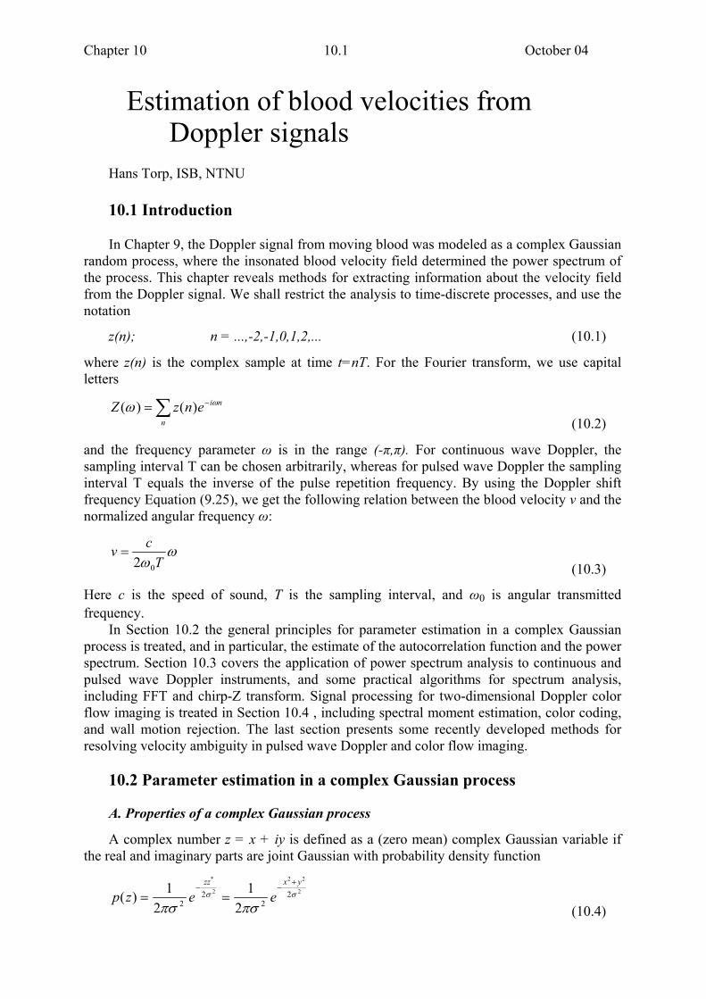
Chapter 10 10.1 October 04 Estimation of blood velocities from Doppler signals Hans Torp, ISB, NTNU 10.1 Introduction In Chapter 9, the Doppler signal from moving blood was modeled as a complex Gaussian random process, where the insonated blood velocity field determined the power spectrum of the process. This chapter reveals methods for extracting information about the velocity field from the Doppler signal. We shall restrict the analysis to time-discrete processes, and use the notation z(n); n = ...,-2,-1,0,1,2,... (10.1) where z(n) is the complex sample at time t=nT. For the Fourier transform, we use capital letters ∑ − = n n i e n z Z ω ω ) ( ) ( (10.2) and the frequency parameter ω is in the range (-π,π). For continuous wave Doppler, the sampling interval T can be chosen arbitrarily, whereas for pulsed wave Doppler the sampling interval T equals the inverse of the pulse repetition frequency. By using the Doppler shift frequency Equation (9.25), we get the following relation between the blood velocity v and the normalized angular frequency ω: ω ω T c v 0 2 = (10.3) Here c is the speed of sound, T is the sampling interval, and ω 0 is angular transmitted frequency. In Section 10.2 the general principles for parameter estimation in a complex Gaussian process is treated, and in particular, the estimate of the autocorrelation function and the power spectrum. Section 10.3 covers the application of power spectrum analysis to continuous and pulsed wave Doppler instruments, and some practical algorithms for spectrum analysis, including FFT and chirp-Z transform. Signal processing for two-dimensional Doppler color flow imaging is treated in Section 10.4 , including spectral moment estimation, color coding, and wall motion rejection. The last section presents some recently developed methods for resolving velocity ambiguity in pulsed wave Doppler and color flow imaging. 10.2 Parameter estimation in a complex Gaussian process A. Properties of a complex Gaussian process A complex number z = x + iy is defined as a (zero mean) complex Gaussian variable if the real and imaginary parts are joint Gaussian with probability density function 2 2 2 2 * 2 2 2 2 2 1 2 1 ) ( σ σ πσ πσ y x zz e e z p + − − = = (10.4)
Transcript of Estimation of blood velocities from Doppler signals
Chapter 10 10.1 October 04
Estimation of blood velocities from Doppler signals Hans Torp, ISB, NTNU 10.1 Introduction In Chapter 9, the Doppler signal from moving blood was modeled as a complex Gaussian
random process, where the insonated blood velocity field determined the power spectrum of the process. This chapter reveals methods for extracting information about the velocity field from the Doppler signal. We shall restrict the analysis to time-discrete processes, and use the notation
z(n); n = ...,-2,-1,0,1,2,... (10.1)
where z(n) is the complex sample at time t=nT. For the Fourier transform, we use capital letters
∑ −=
n
nienzZ ωω )()( (10.2)
and the frequency parameter ω is in the range (-π,π). For continuous wave Doppler, the sampling interval T can be chosen arbitrarily, whereas for pulsed wave Doppler the sampling interval T equals the inverse of the pulse repetition frequency. By using the Doppler shift frequency Equation (9.25), we get the following relation between the blood velocity v and the normalized angular frequency ω:
ωω Tcv
02=
(10.3)
Here c is the speed of sound, T is the sampling interval, and ω0 is angular transmitted frequency.
In Section 10.2 the general principles for parameter estimation in a complex Gaussian process is treated, and in particular, the estimate of the autocorrelation function and the power spectrum. Section 10.3 covers the application of power spectrum analysis to continuous and pulsed wave Doppler instruments, and some practical algorithms for spectrum analysis, including FFT and chirp-Z transform. Signal processing for two-dimensional Doppler color flow imaging is treated in Section 10.4 , including spectral moment estimation, color coding, and wall motion rejection. The last section presents some recently developed methods for resolving velocity ambiguity in pulsed wave Doppler and color flow imaging.
10.2 Parameter estimation in a complex Gaussian process A. Properties of a complex Gaussian process A complex number z = x + iy is defined as a (zero mean) complex Gaussian variable if
the real and imaginary parts are joint Gaussian with probability density function
2
22
2
*
22
22 2
12
1)( σσ
πσπσ
yxzz
eezp+
−−==
(10.4)

Chapter 10 10.2 October 04
Note that the real and imaginary parts are independent random variables, and have equal variance σ. A complex Gaussian vector z = (z1,z2,...,zn) is defined by its probability density function
z
n ezp1Tz
21
)2(1)(
−−=
µ
µπ (10.5)
where the covariance matrix µ is given by µi,j = < zi zj* > (10.6)
and the vector zT is the transposed and complex conjugate of z. Note that the expectation value <zi zj> = 0 for all i,j.
A signal z(t) with a continuous or discrete time parameter t is a complex Gaussian process if every random vector ( z(t1),..., z(tn) ) which is obtained by sampling the process at n points is a complex Gaussian vector. The number n is arbitrarily large. The process z(t) is completely determined by its autocorrelation function, which is a complex valued function of two time parameters
R(t1,t2) = < z(t1) z(t2)* > (10.7) Note that R(t,t) = |z(t)|2 is real valued when t1 = t2. This quantity is the signal power of
the process. If the process is stationary, i.e the stochastic properties are invariant under time shifts, the
autocorrelation is only dependent on the time difference τ= t1-t2. In this case the notation is simplified to
R(τ) = < z(t+τ) z(t)* > (10.8) The power spectrum of a stationary process z(t) is defined as the Fourier transform of the
autocorrelation function
∫= ωτττω ieRdG )()( (10.9)
Figure 10-1.
Power spectrum of a complex process z(t) (above), and its real part (below)
Gz(ω)
ωGx(ω)
ω
x= Re {z}
Chapter 10 10.3 October 04
||-ωo ω
ω
ωo
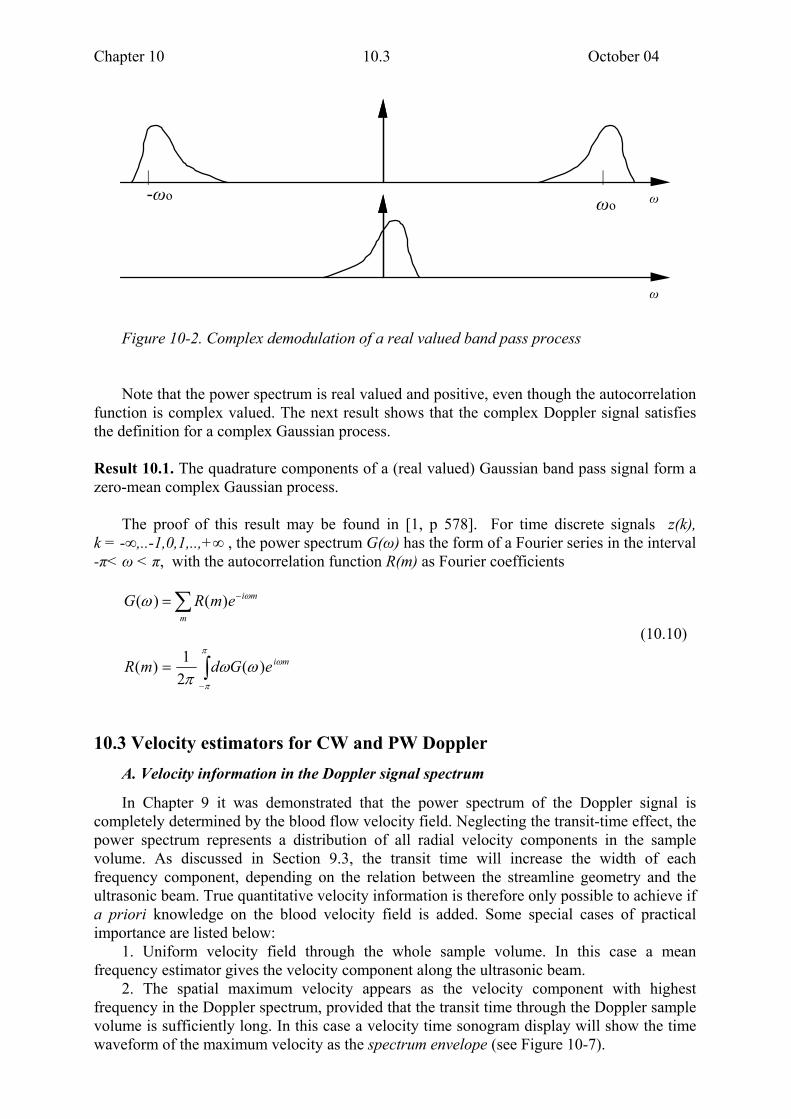
Figure 10-2. Complex demodulation of a real valued band pass process
Note that the power spectrum is real valued and positive, even though the autocorrelation
function is complex valued. The next result shows that the complex Doppler signal satisfies the definition for a complex Gaussian process.
Result 10.1. The quadrature components of a (real valued) Gaussian band pass signal form a zero-mean complex Gaussian process.
The proof of this result may be found in [1, p 578]. For time discrete signals z(k),
k = -∞,..-1,0,1,..,+∞ , the power spectrum G(ω) has the form of a Fourier series in the interval -π< ω < π, with the autocorrelation function R(m) as Fourier coefficients
∑ −=
m
miemRG ωω )()(
(10.10)
∫−
=π
π
ωωωπ
mieGdmR )(21)(
10.3 Velocity estimators for CW and PW Doppler A. Velocity information in the Doppler signal spectrum In Chapter 9 it was demonstrated that the power spectrum of the Doppler signal is
completely determined by the blood flow velocity field. Neglecting the transit-time effect, the power spectrum represents a distribution of all radial velocity components in the sample volume. As discussed in Section 9.3, the transit time will increase the width of each frequency component, depending on the relation between the streamline geometry and the ultrasonic beam. True quantitative velocity information is therefore only possible to achieve if a priori knowledge on the blood velocity field is added. Some special cases of practical importance are listed below:
1. Uniform velocity field through the whole sample volume. In this case a mean frequency estimator gives the velocity component along the ultrasonic beam.
2. The spatial maximum velocity appears as the velocity component with highest frequency in the Doppler spectrum, provided that the transit time through the Doppler sample volume is sufficiently long. In this case a velocity time sonogram display will show the time waveform of the maximum velocity as the spectrum envelope (see Figure 10-7).

Chapter 10 10.4 October 04
In addition, more qualitative information can be extracted from the Doppler spectrum: 3. Signal power (after high pass filtering) above the noise level indicates that there is
moving blood inside the sample volume. 4. Spectral density in the maximum frequency part of the spectrum is related to the
volume of blood moving with high velocity. This gives a qualitative measurement of the severity of a high velocity leakage jet.
These examples show that blood velocity information with practical, clinical importance can be deduced from the Doppler spectrum. This chapter deals with methods to estimate this Doppler spectrum with optimum quality.
B. Spectrum sonogram display In clinical applications of Doppler ultrasound, the periodogram is calculated in real time
on a time/frequency grid, and shown in a gray scale display with time along the horizontal axis, and frequency (or velocity) along the vertical axis. This representation of the Doppler signal is often referred to as a velocity time sonogram, or velocity time spectrum. The gray-level is usually a monotone function of the spectrum value in each point. This transfer function can be adjusted to enhance weak spectral components, like in Figure 10-7.
The spectrum in Figure 10-7 is generated by a blood flow with different velocities along the ultrasonic beam. The most important clinical information is the maximum Doppler shift, which corresponds to the spatial maximum in the velocity field.
_ 4 m/ s
- 0
Figure 10-7. Spectrum sonogram of continuous wave Doppler measurement in a mitral
valve stenosis. The peak spectrum envelope exceeds 4 m/sec. When the ultrasonic beam is directed along a jet stream, the maximum Doppler shift
gives the central velocity in the jet, which is related to the pressure drop along the blood stream line. The maximum Doppler shift as a function of time is often called the spectrum envelope , and can be delineated from the spectrum sonogram, even if the spectral signal-to-noise ratio is low. The bias of the periodogram has little influence on the spectral envelope.
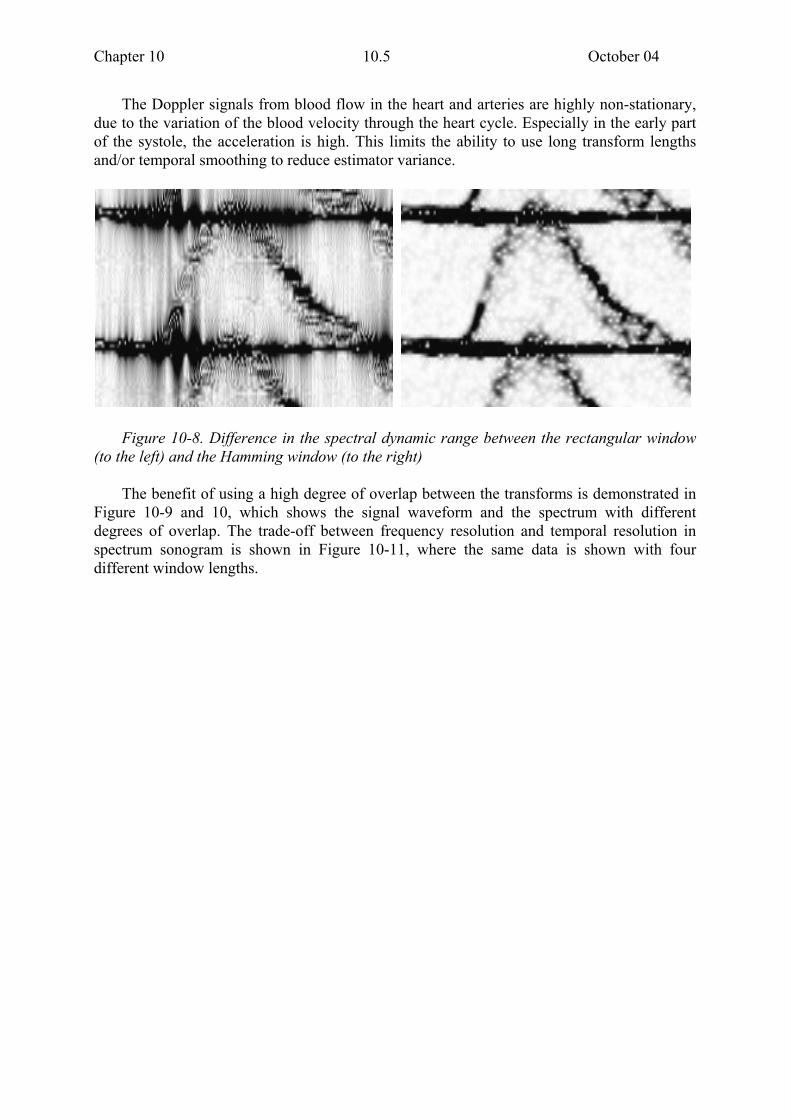
When strong signal components are present, the side lobes from the strong components may interfere with the weaker components near the spectral envelope. In this case, a smooth window function with a low side lobe level is preferred. In Figure 10-8 the difference between a rectangular and a Hamming window is demonstrated in a signal with a strong low frequency component.
Chapter 10 10.5 October 04
The Doppler signals from blood flow in the heart and arteries are highly non-stationary, due to the variation of the blood velocity through the heart cycle. Especially in the early part of the systole, the acceleration is high. This limits the ability to use long transform lengths and/or temporal smoothing to reduce estimator variance.
Figure 10-8. Difference in the spectral dynamic range between the rectangular window
(to the left) and the Hamming window (to the right) The benefit of using a high degree of overlap between the transforms is demonstrated in
Figure 10-9 and 10, which shows the signal waveform and the spectrum with different degrees of overlap. The trade-off between frequency resolution and temporal resolution in spectrum sonogram is shown in Figure 10-11, where the same data is shown with four different window lengths.

Chapter 10 10.6 October 04
window with no overlap
50
window with 50% overlap
50
window with 87% overlap
50
Figure 10-9. Spectrum analysis of a non-stationary signal with different degrees of
overlap. The upper plot is the signal waveform; the window positions are indicated for each spectral line in the lower sonogram displays.
Chapter 10 10.7 October 04
50
50
50
50
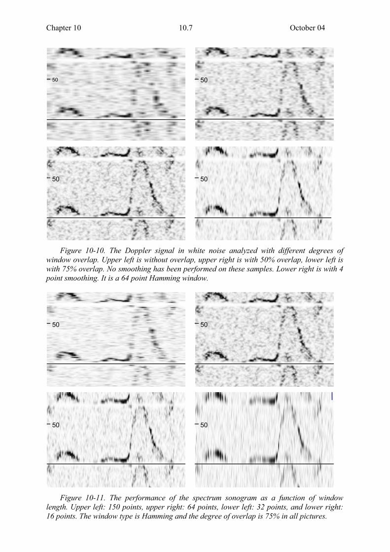
Figure 10-10. The Doppler signal in white noise analyzed with different degrees of
window overlap. Upper left is without overlap, upper right is with 50% overlap, lower left is with 75% overlap. No smoothing has been performed on these samples. Lower right is with 4 point smoothing. It is a 64 point Hamming window.
50
50
50
50
Figure 10-11. The performance of the spectrum sonogram as a function of window
length. Upper left: 150 points, upper right: 64 points, lower left: 32 points, and lower right: 16 points. The window type is Hamming and the degree of overlap is 75% in all pictures.
Chapter 10 10.8 October 04
D. Wall motion rejection Signals from stationary and slowly moving targets like vessel walls and other tissue
structures give an additive low frequency noise (also called clutter noise) which usually is much stronger than the signal from blood. The signal-to-clutter level can be as low as -100 dB [ref] for CW Doppler, 2 MHz ultrasound frequency, but is usually better in PW Doppler, and for higher frequency. Clutter signals are usually suppressed in a high pass filter stage, which is designed with sufficient stop-band damping to minimize the error in the velocity parameter estimator. If a mean frequency estimator is used for blood velocity estimation, the low frequency clutter signal will give a bias towards zero according to
Fractional bias = Pcl / (Pcl+Pb) (10.24) where Pcl and Pb are the signal power from clutter and blood, respectively. In order to
keep the fractional bias below 10%, the signal to clutter level after the high pass filter must be at least +10 dB. For spectrum analysis, a higher clutter level can be accepted, since the different frequency components are separated in the spectral display. However, when the side lobes from clutter signals exceed the receiver noise level, this can be misinterpreted as blood flow signal. For a Hamming window of length N, the spectral density of the side lobes equals the receiver noise level when the noise-to-clutter level equals
Noise-to-clutter level = 10 log(N/2) - 40 [dB] (10.25) For window length N= 64, a signal-to-clutter level after the high pass filter equal to -25
dB will satisfy this requirement. A stop-band requirement of 75-110 dB for the high pass filter means that the filter must
have a relatively long impulse response. However, short transition signals from opening and closing of heart valves may in this case cause ringing in the filters.
10.4 Visualization of 2D Doppler signals
A. Spectral parameters for characterizing blood-flow Visualization of 2D Doppler signals is usually done in combination with ultrasound echo
imaging, as a color-coded overlay to the gray scale tissue image. This modality is therefore called color flow mapping, or color flow imaging. In color flow imaging, the object is to extract information related to the velocity field as reflected in the power spectrum of the Doppler signal at each point of the 2D sector. Compared to conventional Doppler (i.e. CW and PW Doppler technique), the ability to present quantitative velocity information is limited due to
1. Limited information content in the signal, i.e. short observation time, low signal-to- noise ratio, and low Nyquist velocity limit. 2. Insufficient signal processing/display. Full spectrum analysis in each point of the sector is difficult to visualize.
The advantage of color flow imaging, compared to conventional Doppler, lies in the ability to show the spatial distribution of blood-flow, and thereby localize abnormal flow patterns. In order to present 2D Doppler in one image, all velocity information from each
Chapter 10 10.9 October 04
range cell must be compressed into one color value. Usually, three spectral parameters are estimated and combined in a color coding scheme: the signal power, bandwidth, and mean frequency.
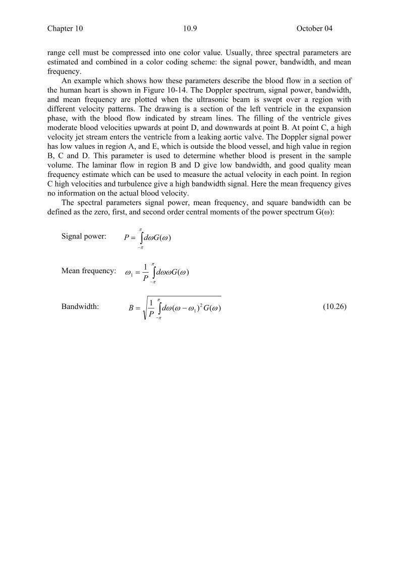
An example which shows how these parameters describe the blood flow in a section of the human heart is shown in Figure 10-14. The Doppler spectrum, signal power, bandwidth, and mean frequency are plotted when the ultrasonic beam is swept over a region with different velocity patterns. The drawing is a section of the left ventricle in the expansion phase, with the blood flow indicated by stream lines. The filling of the ventricle gives moderate blood velocities upwards at point D, and downwards at point B. At point C, a high velocity jet stream enters the ventricle from a leaking aortic valve. The Doppler signal power has low values in region A, and E, which is outside the blood vessel, and high value in region B, C and D. This parameter is used to determine whether blood is present in the sample volume. The laminar flow in region B and D give low bandwidth, and good quality mean frequency estimate which can be used to measure the actual velocity in each point. In region C high velocities and turbulence give a high bandwidth signal. Here the mean frequency gives no information on the actual blood velocity.
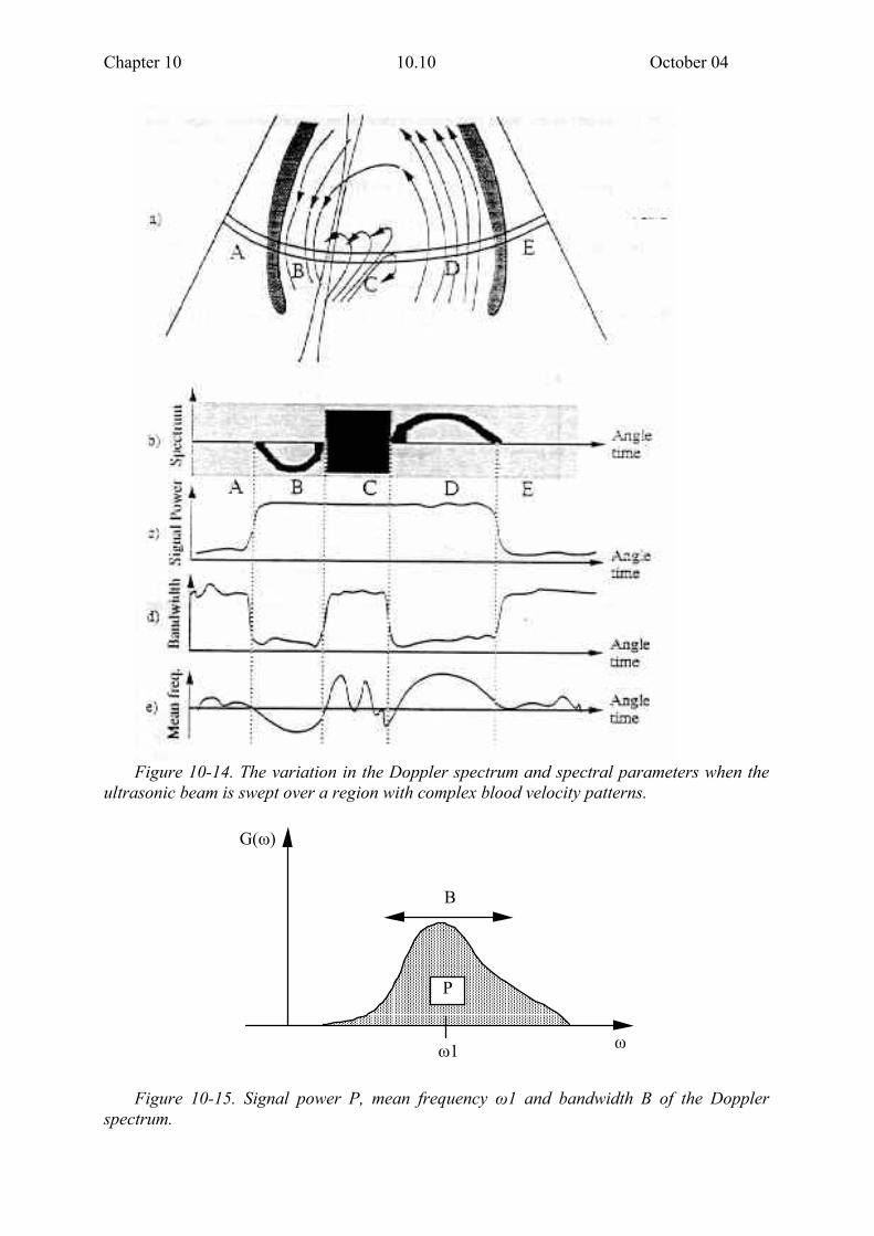
The spectral parameters signal power, mean frequency, and square bandwidth can be defined as the zero, first, and second order central moments of the power spectrum G(ω):
Signal power: ∫−
=π
π
ωω )(GdP
Mean frequency: ∫−
=π
π
ωωωω )(11 Gd
P
Bandwidth: ∫−
−=π
π
ωωωω )()(1 21 Gd
PB (10.26)
Chapter 10 10.10 October 04
Figure 10-14. The variation in the Doppler spectrum and spectral parameters when the
ultrasonic beam is swept over a region with complex blood velocity patterns.
G(ω)
P
B
ω1 ω
Figure 10-15. Signal power P, mean frequency ω1 and bandwidth B of the Doppler
spectrum.

Chapter 10 10.11 October 04
Spectral parameter estimators can be divided into two groups:
1. Frequency domain estimators. These are obtained by substituting a full spectrum estimate into the definition Equation (10.26).
2. Time domain estimators. These are obtained directly from the signal samples, or the autocorrelation estimate.
Frequency domain estimators have the advantage that unwanted signal components (like
white thermal noise, and low frequency wall motion signals) can be subtracted from the spectrum estimate before calculating the actual parameters. Time domain estimators have the advantage of simplicity, which makes them suitable for real-time implementation. In the following, estimators for signal power, mean frequency, and bandwidth will be analyzed.
Signal power estimator An estimator for the signal power P = R(0) can be obtained by setting the lag m=0 in the
autocorrelation estimate defined in Section 10.2. The bias and variance of this signal power estimator is found from Equation (10.13):
∑=
==N
kNN kz
NRP
1
2)(1)0(
0)( =NPBias
BNPGdkR
Nk
NPVar
N
NkN
222 )( )(11)( ≈≈
−= ∫∑
−−=
π
π
ωω
(10.27)
The first approximation is valid for large N, and the second approximation shows the
dependency on the bandwidth B. Note that the variance of PN decreases with increasing bandwidth B.
Mean frequency estimator The autocorrelation function with lag m=1 can be expressed as an integral over ω of the
complex exponential exp(iω), weighted by the power spectrum G(ω), Equation (10.10)
∫−
=π
π
ωωωπ
ieGdR )(21)1( (10.28)
In Figure 10-16 the power spectrum G(ω) is displayed as a polar plot, demonstrating that
the complex number R(1) represents the center of gravity of the trace {G(ω)exp(i ω); -π< ω <π} in the polar diagram. The phase of R(1) will therefore be an approximation of the mean frequency, as defined in Equation(10.26). This can be verified by a power series expansion of exp(i ω) in the point ω 1=phase(R(1)).

Chapter 10 10.12 October 04
}211{
} .... )(21)(1){(
)()1(
2
211
)(
1
1
11
BPe
iGde
eGdeR
i
i
ii
−≈
+−−−+=
=
∫
∫
−
−
−
ω
π
π
ω
π
π
ωωω
ωωωωωω
ωω
∫−
−=π
π
ωωωω )()(1 21
2 GdP
B (10.29)
The last approximation is valid when G(ω) vanishes outside a small interval around
ω=ω1. P is the signal power, and B is the RMS-bandwidth. A mean frequency estimator is obtained by using the autocorrelation estimator RN(1) ,
with m=1.
==
)}1(Re{)}1(Im{arctan))1((1
N
NNN R
RRphaseω
∑=
+=N
kN kzkz
NR
1
*)()1(1
(10.30) For narrow band signals and large N, the estimator bias ≈ 0, and the variance is
approximately given by
NBVar N
2
1 )( ≈ω (10.31)
Note that the variance increases with increasing bandwidth B, in contrast to the variance of the signal power estimate, which decreases with increasing bandwidth.
Bandwidth estimator
)0(|)1(|12
N
NN R
RB −= (10.32)
For white noise, corresponding to |R(1)| = 0, the RMS bandwidth B=π/sqrt(3)=1.84.
Using (10.32) gives the value sqrt(2) which is 30% too low. In Figure 10-17, the expectation value and variance for the normalized autocorrelation
function estimator are indicated in the complex plane for two different signals, one with narrow bandwidth, and one with broad bandwidth.
The normalized autocorrelation function is defined as
)0()()(
RmRm =ρ
(10.33)

Chapter 10 10.13 October 04
)exp(i )G( ωω
∫ )exp(i )G( d ωωωim{R(1)}
re{R(1)}π
- πG(ω)
πω- π
Figure 10-16. Power spectrum G(ω) to the right, and its polar presentation and the
complex autocorrelation R(1) to the left.
im{ρ(1)}
re{ρ (1)}
Narrow band signal
Broad band signal
1
i
Figure 10-17. The estimate of the normalized autocorrelation function ρ(1) for two
different signals. Expectation values are indicated by the arrows, and distribution around the mean values are indicated by ellipses.
Chapter 10 10.14 October 04
From Equation (10.29) the following relation between the absolute value |R(1)| and the bandwidth parameter B is valid, when the bandwidth is low:
2
211 )1()1( B
PR
−≈=ρ (10.34)
By inverting Equation (10.34), and inserting the autocorrelation estimate for R(1) and
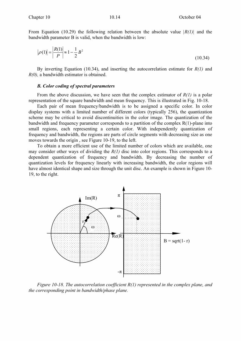
R(0), a bandwidth estimator is obtained. B. Color coding of spectral parameters From the above discussion, we have seen that the complex estimator of R(1) is a polar
representation of the square bandwidth and mean frequency. This is illustrated in Fig. 10-18. Each pair of mean frequency/bandwidth is to be assigned a specific color. In color
display systems with a limited number of different colors (typically 256), the quantization scheme may be critical to avoid discontinuities in the color image. The quantization of the bandwidth and frequency parameter corresponds to a partition of the complex R(1)-plane into small regions, each representing a certain color. With independently quantization of frequency and bandwidth, the regions are parts of circle segments with decreasing size as one moves towards the origin , see Figure 10-19, to the left.
To obtain a more efficient use of the limited number of colors which are available, one may consider other ways of dividing the R(1) disc into color regions. This corresponds to a dependent quantization of frequency and bandwidth. By decreasing the number of quantization levels for frequency linearly with increasing bandwidth, the color regions will have almost identical shape and size through the unit disc. An example is shown in Figure 10-19, to the right.
ω
π
-π
ω
Re(R)
Im(R)
r
B = sqrt(1- r)
Figure 10-18. The autocorrelation coefficient R(1) represented in the complex plane, and
the corresponding point in bandwidth/phase plane.
Chapter 10 10.15 October 04
Im(R)
Re(R)
ω
b
Im(R)
Re(R)
ω
b
Figure 10-19. Two different quantization schemes for center-frequency/bandwidth.. To the left : Independent quantization with 7*18 levels. To the right: Dependent quantization with 7*36 levels. Both give a total number of 126 values.
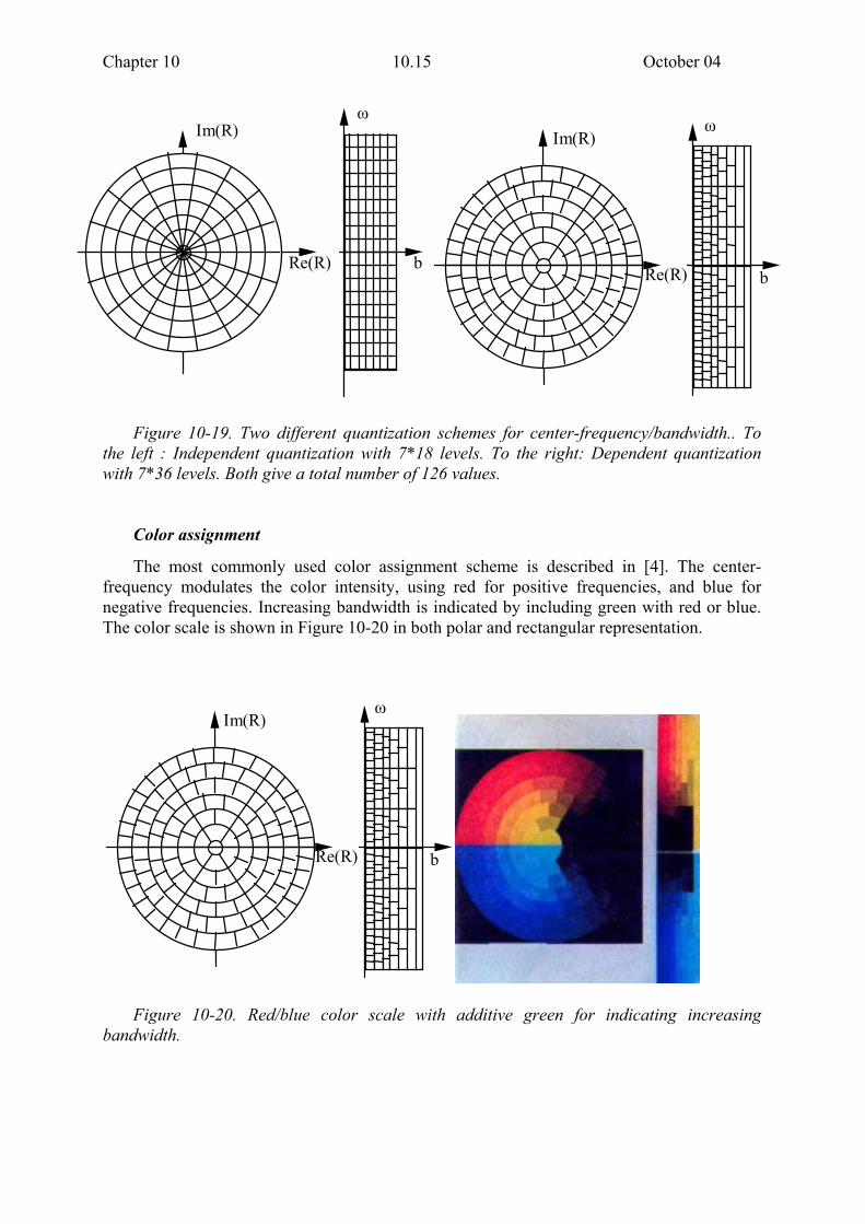
Color assignment The most commonly used color assignment scheme is described in [4]. The center-
frequency modulates the color intensity, using red for positive frequencies, and blue for negative frequencies. Increasing bandwidth is indicated by including green with red or blue. The color scale is shown in Figure 10-20 in both polar and rectangular representation.
Im(R)
Re(R)
ω
b
Figure 10-20. Red/blue color scale with additive green for indicating increasing
bandwidth.
Chapter 10 10.16 October 04
Ao
LV
LA
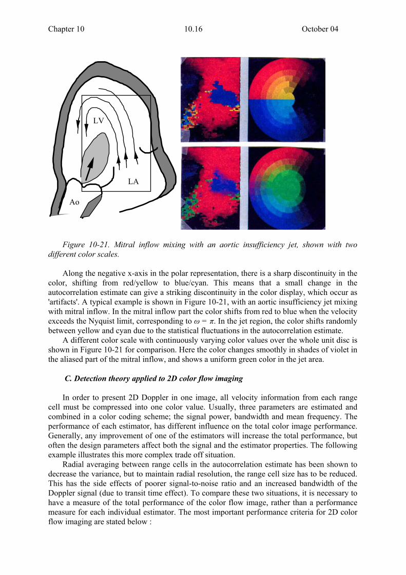
Figure 10-21. Mitral inflow mixing with an aortic insufficiency jet, shown with two
different color scales. Along the negative x-axis in the polar representation, there is a sharp discontinuity in the
color, shifting from red/yellow to blue/cyan. This means that a small change in the autocorrelation estimate can give a striking discontinuity in the color display, which occur as 'artifacts'. A typical example is shown in Figure 10-21, with an aortic insufficiency jet mixing with mitral inflow. In the mitral inflow part the color shifts from red to blue when the velocity exceeds the Nyquist limit, corresponding to ω = π. In the jet region, the color shifts randomly between yellow and cyan due to the statistical fluctuations in the autocorrelation estimate.
A different color scale with continuously varying color values over the whole unit disc is shown in Figure 10-21 for comparison. Here the color changes smoothly in shades of violet in the aliased part of the mitral inflow, and shows a uniform green color in the jet area.
C. Detection theory applied to 2D color flow imaging In order to present 2D Doppler in one image, all velocity information from each range
cell must be compressed into one color value. Usually, three parameters are estimated and combined in a color coding scheme; the signal power, bandwidth and mean frequency. The performance of each estimator, has different influence on the total color image performance. Generally, any improvement of one of the estimators will increase the total performance, but often the design parameters affect both the signal and the estimator properties. The following example illustrates this more complex trade off situation.
Radial averaging between range cells in the autocorrelation estimate has been shown to decrease the variance, but to maintain radial resolution, the range cell size has to be reduced. This has the side effects of poorer signal-to-noise ratio and an increased bandwidth of the Doppler signal (due to transit time effect). To compare these two situations, it is necessary to have a measure of the total performance of the color flow image, rather than a performance measure for each individual estimator. The most important performance criteria for 2D color flow imaging are stated below :
Chapter 10 10.17 October 04
1. To detect regions with blood flow, and discriminate them from regions without blood flow.
2. To discriminate between 'normal' and 'disturbed' blood-flow.
3. To estimate the radial velocity component with minimum bias and variance.
The estimated mean frequency gives the radial velocity component in regions with normal flow. The intensity and bandwidth parameters have no direct relevance, other than to help make a decision about what kind of region each point in the image belongs to. Rather than searching for minimum variance estimators, the problem may be stated as a multi-hypothesis decision problem. To design the optimum decision rule and evaluate the performance, detailed knowledge of the statistical properties of the estimated parameters under each hypothesis is required.
In order to treat this problem mathematically, a simplified situation is considered. The insonified area is divided into three regions:
Region 0: No flow Region 1: Normal flow Region 2: Disturbed flow Since the Doppler signal is characterized by its power spectrum (or autocorrelation
function), the regions are here defined in terms of their effect on the Doppler spectrum, rather than their true hemodynamic properties.
Normal flow means rectilinear flow within the sample volume with velocity low enough
to give a moderate transit time broadening in the Doppler spectrum, and high enough to exceed the high-pass filter cutoff frequency. The bandwidth should be low enough to make sufficient good center frequency estimate.
Disturbed flow includes two different types of flow. One is high velocity rectilinear
flow, where the transit time effect causes a large broadening of the Doppler signal spectrum. The other is turbulent flow giving signal components distributed all over the frequency range in the power spectrum. In both cases the result is a broadband Doppler signal, where the center frequency gives little information. In a typical jet flow region, there is a core with high velocities, surrounded by turbulent flow. This gives a connected area of 'disturbed flow', characterized by a broadband, almost white noise Doppler spectrum.
No flow. Thermal noise in the receiver will add a white noise component with constant
intensity to the Doppler signal. When no flow is present, or the flow velocity is too low, or too weak a signal, this receiver noise will dominate. In addition, some low frequency components from tissue may be present due to insufficient high-pass filtering.
The problem will be analyzed by classical detection theory with three hypotheses, each
characterized by a family of power spectra:
H0 : No flow. High-pass filtered white noise with low intensity H1 : Normal flow. Narrow band signal H2 : Disturbed flow. High-pass filtered white noise with increased intensity
An example with typical power spectra under the three hypotheses is shown in Figure 10-22.

Chapter 10 10.18 October 04
Figure 10-22. Color flow image of an aortic regurgitant jet (green area) mixing into mitral inflow (red area). Power spectra are estimated from the signal and displayed in a polar plot in the jet area (upper left), mitral inflow area (upper right), and area with no blood flow (lower left). The red arrow indicates the signal intensity, and the green arrow is the normalized autocorrelation function of unity lag.
Chapter 10 10.19 October 04
There are 4 basic components in a decision-theory problem [5, pp.19] 1. A source which generates one out of a finite number of choices (hypotheses) 2. The observation space 3. The probabilistic transition mechanism between source and observation
space. 4. The decision rule For this detection problem, the source is a two-dimensional slice of the blood flow
velocity field, divided into three regions. The probabilistic transition mechanism is determined by the conditional probability density functions p(x|Hi) under hypothesis Hi i=0,1,2 for the measurement vector x, which is a point in the observation space. The measurement vector x could be a segment of the Doppler signal, or a set of estimators on the Doppler signal (for instance the autocorrelation estimate) .
If the a priori probability P(Hi) for each hypothesis Hi is known, the a posteriori probability P(Hi|x) follows by Baye's law
0,1,2=i , )(
)()()(
xpHPHxp
xHP iii =
∑=
=2
0
)()()(j
jj HPHxpxp (10.35)
The sum of the three a posteriori probabilities must equal one, so all information is contained in P(H1|x) and P(H2|x). In classical detection theory these quantities are used to form a decision rule. A special case is the minimum total probability of error test where the decision rule is to choose the one with maximum a posteriori probability [6]. Applied to color flow imaging, the hypothesis H1 and H2 could be assigned two different colors c1 and c2, and H0 could be assigned the color black (or no color) . By calculating P(H1|x) and P(H2|x) in each point of the picture, picking out the color corresponding to the largest, a minimum total probability of error color scheme is obtained .
A more refined color assignment is possible to achieve by mixing the colors c1 and c2 with weights equal to the corresponding a posteriori probabilities.
)()( 2211 xHpcxHpccolor += (10.36)
This will give a color close to c1 or c2 when one of them has a high a posteriori
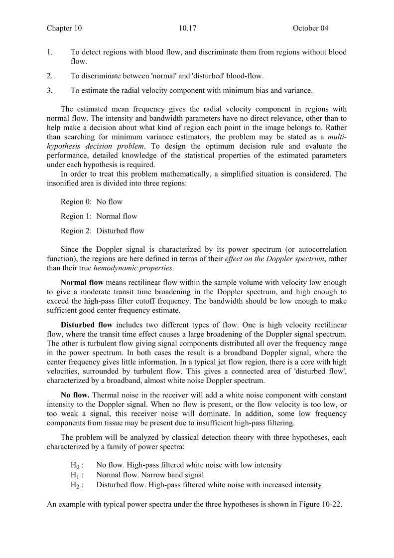
probability, and a color close to black, when H0 is likely to be true. D. Hypothesis test with the intensity/bandwidth estimates as a 2D observation space A three-hypotheses detection scheme is worked out in detail, using the signal power, and
bandwidth as a two-dimensional observation space. As can be seen from Figure 10-23, there is a distinct correlation between these two random variables, which indicates that a combination of the two parameters should be used in the decision rule.
Chapter 10 10.20 October 04
•• •
•••
••
•
•• •• • •
••••
••
•
••••
•
••
•••
•
•
•
• • ••
•
•
•
•
•••
••••
••
•••• •
••
••••
••
•••
•••
•
• H1
H2
H0
•
•
•
y
x
Figure 10-23. Scatter plot of x=log bandwidth, y = log intensity, under the three hypotheses H0, H1 and H2 . The conditional PDF under each hypothesis is fitted to a two-dimensional Gaussian distribution, which is indicated by the e-1 contour.
To compute the a posteriori probability under each hypothesis, the conditional
probability density functions is needed. These may be found directly by computer simulations, but very long time series is needed to get a reliable result. Therefore a parametric representation of the PDF under each hypothesis is preferred. By taking a logarithm of the signal power and bandwidth, the two-dimensional scatter plot shows a fairly good match with Gaussian distribution, under all three hypotheses, see Figure 10-23. The parameters characterizing the PDF (probability density function) are estimated from computer simulated time series with standard methods.
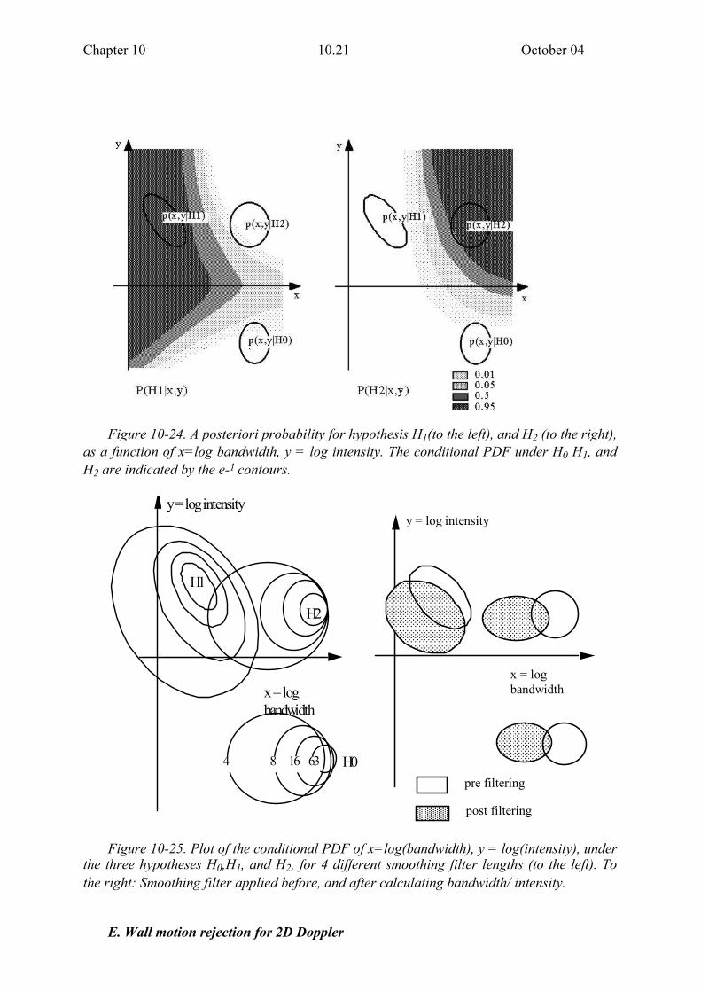
From the conditional PDF under each hypothesis, the a posteriori probabilities can be calculated, using Equation (1). This has been done for the example in Figure 10-23, assuming equal a priori probabilities. A posteriori probability as a function of (x, y) is displayed in shades of gray in Figure 10-24, for hypotheses H1 and H2.
In the next figure, the effect of a smoothing filter on the autocorrelation estimate is demonstrated. One observes that the variance decreases with filter length, but also the mean values change, so that the distance between the PDF’s under the different hypothesis increases. A smoothing filter applied after the nonlinear operation of calculating bandwidth/log intensity will not have the same effect on the mean values, and will therefore give poorer results. It is interesting to make quantitative comparisons between the two different filtering approaches (here called pre- and post filtering). In Figure 10-25 to the right, 16 point pre-filtering is compared with 4-point pre-filtering, followed by post filtering to yield the same total filter length.
Chapter 10 10.21 October 04
Figure 10-24. A posteriori probability for hypothesis H1(to the left), and H2 (to the right),
as a function of x=log bandwidth, y = log intensity. The conditional PDF under H0 H1, and H2 are indicated by the e-1 contours.
4 8 16 63
y = log intensity
x = logbandwidth
H1
H2
H0
y = log intensity
x = logbandwidth
pre filtering
post filtering Figure 10-25. Plot of the conditional PDF of x=log(bandwidth), y = log(intensity), under
the three hypotheses H0,H1, and H2, for 4 different smoothing filter lengths (to the left). To the right: Smoothing filter applied before, and after calculating bandwidth/ intensity.
E. Wall motion rejection for 2D Doppler
Chapter 10 10.22 October 04
The first multi-gated Doppler used a separate signal processing unit for each depth
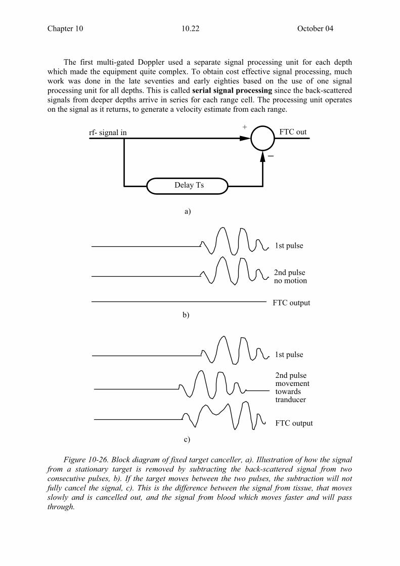
which made the equipment quite complex. To obtain cost effective signal processing, much work was done in the late seventies and early eighties based on the use of one signal processing unit for all depths. This is called serial signal processing since the back-scattered signals from deeper depths arrive in series for each range cell. The processing unit operates on the signal as it returns, to generate a velocity estimate from each range.
Delay Ts
rf- signal in+ FTC out
FTC output
2nd pulse no motion
1st pulse
2nd pulse movement towards tranducer
FTC output
a)
b)
1st pulse
c) Figure 10-26. Block diagram of fixed target canceller, a). Illustration of how the signal
from a stationary target is removed by subtracting the back-scattered signal from two consecutive pulses, b). If the target moves between the two pulses, the subtraction will not fully cancel the signal, c). This is the difference between the signal from tissue, that moves slowly and is cancelled out, and the signal from blood which moves faster and will pass through.
Chapter 10 10.23 October 04
The first experiments with serial processing were presented in 1975 using the moving target indicator (MTI) technique, that was previously developed for radar and sonar systems. In the simplest form of this technique, the back-scattered signals from two consecutive ultrasound pulses are subtracted so that the signals from targets that do not move are removed as illustrated in Figure 10-26b. This is called fixed target canceller (FTC). For peripheral vessels where the tissue structures are moving slowly, this method removes the signals from the tissue so that we are left with the signals from the blood, which are moving targets (hence the name MTI). The blood velocity profile along the beam is then estimated from the Doppler frequency.
The FTC is the same as the high pass filter for the PW/CW Doppler as described in Section 2.6B. It removes the low Doppler frequencies from the tissues that move slowly and allows the high Doppler frequencies from the blood which moves faster to pass through. We therefore use the term FTC and high pass filter interchangeably.
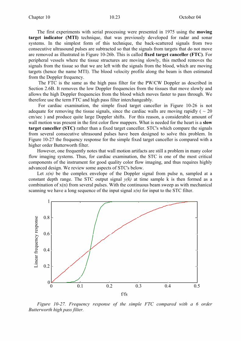
For cardiac examination, the simple fixed target canceller in Figure 10-26 is not adequate for removing the tissue signals, since the cardiac walls are moving rapidly ( ~ 20 cm/sec ) and produce quite large Doppler shifts. For this reason, a considerable amount of wall motion was present in the first color flow mappers. What is needed for the heart is a slow target canceller (STC) rather than a fixed target canceller. STC's which compare the signals from several consecutive ultrasound pulses have been designed to solve this problem. In Figure 10-27 the frequency response for the simple fixed target canceller is compared with a higher order Butterworth filter.
However, one frequently notes that wall motion artifacts are still a problem in many color flow imaging systems. Thus, for cardiac examination, the STC is one of the most critical components of the instrument for good quality color flow imaging, and thus requires highly advanced design. We review some aspects of STC's below.
Let x(n) be the complex envelope of the Doppler signal from pulse n, sampled at a constant depth range. The STC output signal y(k) at time sample k is then formed as a combination of x(n) from several pulses. With the continuous beam sweep as with mechanical scanning we have a long sequence of the input signal x(n) for input to the STC filter.
0
0.2
0.4
0.6
0.8
1
0 0.1 0.2 0.3 0.4 0.5
f/fs
Line
ar fr
eque
ncy
resp
onse
Figure 10-27. Frequency response of the simple FTC compared with a 6 order
Butterworth high pass filter.

Chapter 10 10.24 October 04
A standard linear time invariant filter of the type y(k) = h(n)x(k − n)
n∑ (10.37)
is then often used. The filter impulse response is h(n), which can be both of the IIR
(infinite impulse response) and the FIR (finite impulse response) type. The filter is designed as a standard high pass filter that attenuates the low frequency Doppler shifts from the tissue.
With electronic scanning, the beam direction is stepped in discrete directions, while transmitting several pulses for each direction. This produces a finite number of signal samples (x(1),..., x(N)) for each beam direction. Using the time invariant filter, we will get a settling time of the filter for each new beam direction, as illustrated in Figure 10-28. This can partly be avoided by using a time variant filter, where the impulse response is different for each sample of the output signal. The filter should however be linear, in order to avoid inter-modulation between the tissue signal and the blood signal. Since the filter is linear, it can be described mathematically as a linear transform on the N dimensional complex vector space CN, and can therefore be performed by multiplying the input vector with a NxN transformation matrix A = {a(n,m)}
Input vector: x = (x(1), ... ., x(N))Output vector: y = (y(1), .. .., y(N)) = Ax
y(k) = a(n,k)x(n)n=1
N
∑ ; k = 1,.., N
(10.38)
Signal discontinuity causes ringing in high-pass filters
Raw signal from beam k
Signal after high-pass filter
Lost settling time
Figure 10-28. The settling time of the high pass filter for a phased array scanner.
Chapter 10 10.25 October 04
A time invariant FIR filter with an impulse response h(n), n=0,1,..,M has a filter matrix given by:
a(n,k) =h(k − n) for k ≥ n and k > M0 elsewhere
(10.39)
Note that the first M samples in the output signal is zero. The frequency response of the
FIR filter can be defined by the Fourier transform of the impulse response h(n). This definition of the frequency response can not be applied to the general linear filter. However, a frequency response function Ho(ω) can be defined as the power of the output signal when the input is a complex harmonic signal.
x(k) = eikω ; k =1, 2,.. , N
y(k) = a(n,k)einω
n=1
N
∑ ≡ Ak (ω )
H0 (ω ) ≡ 1N yω (k)
2
k =1
N
∑ = 1N Ak(ω )
2
k =1
N
∑
(10.40)
The quantity Ak(ω) is the Fourier transform of row number k in the filter matrix. Since
the transform is linear, a constant phase shift of the input signal will give a factor eiω with unit length, and will therefore not influence the output power. This means that the frequency response in (10.40) is well defined. This is a unique property for complex base band signals.
For real valued signals, an ensemble average over all possible phases of the input signal is necessarily in order to obtain a well defined frequency response [4]. In the complex case, the power of the real- and imaginary parts both varies with the phase of the input signal in such a way that the sum is constant. Note that for FIR filters, the frequency response defined in (10.40) coincide with the usual definition.
If the filter matrix elements attain complex values, non-symmetric frequency responses can be obtained, which is useful for adaptive clutter filters, where the Doppler shift of the tissue signal is estimated from the signal.
Unlike the linear convolution filter, the output will not in general be a complex harmonic sequence, but may contain frequency components which are not present in the input signal. This property can cause severe problems in color flow imaging, where strong clutter signals may generate higher frequency components which affect both the center frequency and the bandwidth estimate. This frequency distortion is only absent for FIR-filters, where the number of non-zero output samples must be reduced to N-M, where M is the FIR filter order. A reduction of the number of output samples will increase the variance in the velocity parameter estimates, and should therefore be minimized. Several methods have been proposed for reducing the "ring-down time" in the filter [10]. The basic idea is to extend the signal interval by some sort of prediction, followed by a FIR or IIR convolution filter. As long as the predicted values are formed by linear combinations of the original input signal, the total filter operation will still be linear, and can therefore be performed by a matrix multiplication.
Another approach was taken by Hoeks et. al [4], where the clutter signal was estimated by a least square fitting to a straight line, and then subtracted from the input signal. This is one example from a class of filters which is called regression filters. If we assume that the clutter signal is contained in a subspace κ of CN, the projection transform Pκ from CN into κ gives the least square fit to the clutter component. The clutter filter will then have the form A = I - Pκ, which is a projection into the orthogonal complement of κ
Chapter 10 10.26 October 04
0
0.2
0.4
0.6
0.8
1
0 0.1 0.2 0.3 0.4 0.5
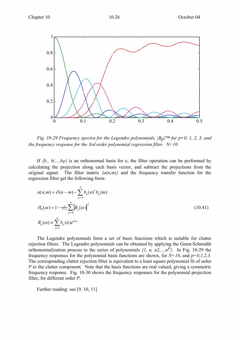
Fig. 10-29 Frequency spectra for the Legendre polynomials, |Bp|™ for p=0, 1, 2, 3, and
the frequency response for the 3rd order polynomial regression filter. N=10.
If {b‚, b⁄,...,bP} is an orthonormal basis for κ, the filter operation can be performed by
calculating the projection along each basis vector, and subtract the projections from the original signal. The filter matrix {a(n,m)} and the frequency transfer function for the regression filter get the following form:
a(n,m) = δ (n − m) − bp(n)* bp (m)p= 0
P
∑
H0 (ω ) =1 − 1P+1 Bp(ω )
2
p= 0
P
∑
Bp (ω) ≡ bp (n)einω
n=1
N
∑
(10.41)
The Legendre polynomials form a set of basis functions which is suitable for clutter
rejection filters. The Legendre polynomials can be obtained by applying the Gram-Schmidth orthonormalization process to the series of polynomials {1, n, n2,...,nP}. In Fig. 10-29 the frequency responses for the polynomial basis functions are shown, for N=10, and p=0,1,2,3. The corresponding clutter rejection filter is equivalent to a least square polynomial fit of order P to the clutter component. Note that the basis functions are real valued, giving a symmetric frequency response. Fig. 10-30 shows the frequency responses for the polynomial projection filter, for different order P.
Further reading: see [9, 10, 11]

Chapter 10 10.27 October 04
-60
-50
-40
-30
-20
-10
0
0 0.1 0.2 0.3 0.4 0.5
frequency
Ho
[dB
]
Figure 10-30. Frequency response for the Legendre polynomial regression filter, with
order P=0, 1, 2, 3, and 4. N=10. 10.5 Resolving velocity ambiguity in pulsed wave Doppler A. A two-dimensional stochastic model for the Doppler signal In Chapter 9 the autocorrelation for the Doppler signal from one range gate was derived
formally from a random scattering model. This model has been extended to a two-dimensional Gaussian process, to also include the correlation of the signal in the depth range direction [4, 6, 7]. The received RF signal from a single scatterer passing through the ultrasonic beam is shown in Figure 10-31.
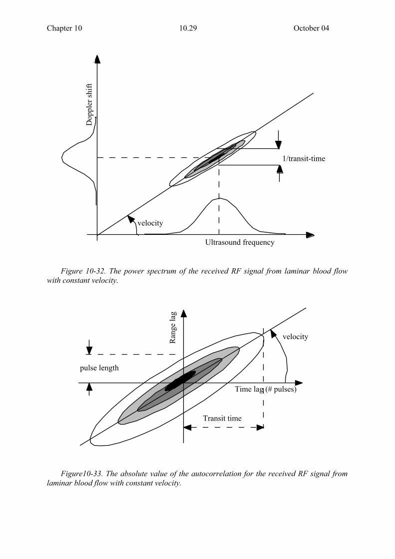
By a two-dimensional Fourier transform of the received RF signal, the power spectrum will appear as indicated in Figure 10-32. The horizontal range axis is transformed to the horisontal, transmitted frequency axis, and the vertical axis is transformed to Doppler frequency shift. The two dimensional power spectrum shows how each frequency component of the transmitted signal create a Doppler shift, proportional to the velocity and the transmitted frequency, as stated by the Doppler equation. The power spectrum will be concentrated close to the "iso-velocity line" in the (ω1,ω2) plane given by the Doppler equation.
ω2 = 2 v/c ω1 (10.42) In Figure 10-33 the magnitude of the corresponding autocorrelation function is drawn. It
is indicated in the figure how the pulse length, blood velocity, and the transit time through the beam, determine the form of the autocorrelation function.

Chapter 10 10.28 October 04
beam profile
v
v l
r
pulse 1
pulse 2
pulse 3
pulse 4
Signal from one range
Tran
sduc
er
Figure 10-31. The received signal from a point scatterer moving through the ultrasonic
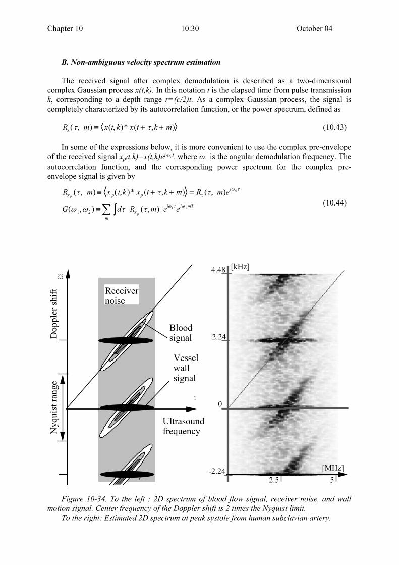
beam. Due to the time discrete nature of the signal in the range direction, the two-dimensional
power spectrum will appear repetitive in the vertical direction, with a distance equal to the pulse repetition frequency. This is shown in Figure 10-34, where the three components of the received signal can be recognized. These are:
1. Signal from slowly moving tissue, giving the horizontal lines
2. Signal from moving blood giving the skewed lines
3. Receiver thermal noise, which gives a constant background level over the entire frequency range of the front end. To the right in Figure 10-34, the 2D power spectrum estimate of the signal from blood in
a human blood vessel (subclavian artery) is shown.
Chapter 10 10.29 October 04
Ultrasound frequency
Dop
pler
shift
velocity
1/transit-time
Figure 10-32. The power spectrum of the received RF signal from laminar blood flow
with constant velocity.
Time lag (# pulses)
velocity
pulse length
Ran
ge la
g
Transit time
Figure10-33. The absolute value of the autocorrelation for the received RF signal from
laminar blood flow with constant velocity.
Chapter 10 10.30 October 04
B. Non-ambiguous velocity spectrum estimation The received signal after complex demodulation is described as a two-dimensional
complex Gaussian process x(t,k). In this notation t is the elapsed time from pulse transmission k, corresponding to a depth range r=(c/2)t. As a complex Gaussian process, the signal is completely characterized by its autocorrelation function, or the power spectrum, defined as
Rx(τ, m) ≡ x(t, k)* x(t + τ,k + m) (10.43) In some of the expressions below, it is more convenient to use the complex pre-envelope
of the received signal xp(t,k)=x(t,k)eiω‚t, where ω‚ is the angular demodulation frequency. The autocorrelation function, and the corresponding power spectrum for the complex pre-envelope signal is given by
Rx p
(τ, m) ≡ x p(t,k )* xp (t + τ,k + m) = Rx (τ, m)eiω 0τ
G(ω1,ω2 ) ≡ dτ∫m∑ Rx p
(τ, m) eiω1τeiω 2mT (10.44)
�‚
Ultrasound frequency
Dop
pler
shift
Vessel wall signal
Blood signal
Receiver noise
�¹
�¤
Nyq
uist
rang
e
[kHz]
2.24
4.48
0
-2.242.5 5
[MHz]
Figure 10-34. To the left : 2D spectrum of blood flow signal, receiver noise, and wall motion signal. Center frequency of the Doppler shift is 2 times the Nyquist limit.
To the right: Estimated 2D spectrum at peak systole from human subclavian artery.

Chapter 10 10.31 October 04
Due to the sampled nature of the Doppler signal, the power spectrum G(ω1,ω2) is periodic in the ω2 variable, and may therefore be written as a sum of copies of the non-aliased part G(ω1,ω2) with distances equal to the angular pulse repetition frequency 2π/T. The pulse repetition period is T.
G(ω1,ω2 ) = G0(ω1,ω2 + n 2π
T )n
∑
G0 (ω1,ω2 ) ≡ dm dτ Rx p(τ, m)eiω 1τ∫∫ eiω 2mT
(10.45)
The autocorrelation function is determined by the point echo response from blood s(t)
(including frequency dependent attenuation and scattering), and the transversal two-way beam sensitivity function b(d), where d is the distance from the ultrasonic beam center axis. If the blood velocity field is stationary and uniform, the autocorrelation function takes on the form
Rx p
(τ, m; vr , vt) = s2 (τ − mδ v r) • b2 (vtTm)
δ vr = −
2vrTc
(10.46)
where vr and vt are the velocity components in the radial (along the ultrasonic beam) and lateral (transversal to the ultrasonic beam) direction. The subscript s2 and b2 is a short notation for the autocorrelation operator applied to s and b respectively, T is the pulse repetition period, and c is the speed of sound. The radial velocity component causes a change in arrival time from pulse to pulse, denoted ∂v . The minus sign in (10.46) is due to the convention that positive velocity means towards the transducer.
The non aliased part of the spectrum G(ω1,ω2) is obtained by combining equations (10.45) and (10.46)
G0 (ω1,ω2 ) = S(ω1)
2 • B 1
vt(ω 2 − 2v r
c ω1)( ) 2 (10.47)
where S(ω) and B(ω) are the Fourier transforms of s and b respectively. The frequency response S(ω) limits the spectral bandwidth in the ω1 direction. The argument of B is zero along a straight line through the origin in the (ω1,ω2) plane, which represents the Doppler shift equation. Since B is a low pass function, the spectral energy is concentrated along this line, and the bandwidth in the ω2-direction is proportional to the lateral velocity component.
If there is more than one velocity component inside the ultrasonic beam, the total signal power spectrum is obtained by an integration over the velocity, weighted by a velocity distribution function p(v)=p(vr,vt).
( )2
12
212
1
2121
)(),( )(
), ;,(),( ),(
ωωω
ωωωω
cv
vtrtr
trtrtr
r
tBvvpdvdvS
vvGvvpdvdvG
−=
=
∫∫
(10.48) The object of velocity spectrum analysis is to derive the velocity distribution from the
signal. However, the spectral width can also be caused by a spread in the radial velocity components. In the following, the angle between the ultrasonic beam and the blood velocity field, ø, is assumed to be known, and constant through the sample volume. In this case, the velocity distribution is described by the distribution of the radial component. The subscript r is omitted in the following expressions, and Equation (10.48) is simplified to

Chapter 10 10.32 October 04
))tan(, ;,()( ),( 2121 θωωωω vvGvpdvG ∫= (10.49)
In Figure 10-34 the two-dimensional power spectrum is shown for ultrasound RF-signals collected from a human artery. Note that the spectral components for blood can be clearly distinguished from the tissue signal, although the Doppler center frequency are the same for the two signal components.
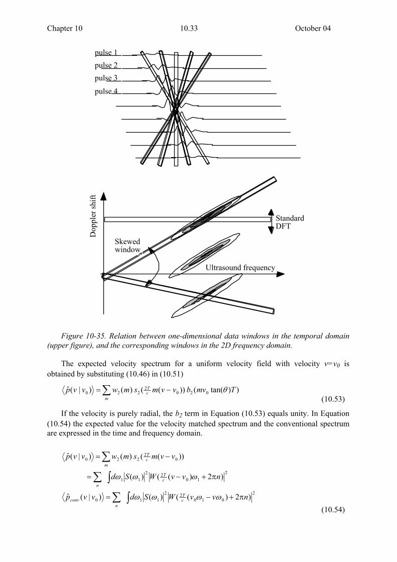
By keeping ω1 constant in Equation (10.49), one gets the (narrow band) Doppler spectrum which represents a blurred version of the velocity distribution function p(vr). This spectrum is subject to frequency aliasing for velocities exceeding the Nyquist limit. However, this limit is different for each ω1, and this can be utilized to resolve frequency ambiguity. By integrating the 2D power spectrum along the iso-velocity lines for each velocity, a velocity spectrum with suppressed aliasing is obtained. The 2D power spectrum can be estimated by the 2D FFT technique, and the integration along the iso-velocity lines can be performed by integrating the frequency components in the 2D frequency plane, see Figure 10-35, lower part. An algorithm based on this principle was proposed by Wilson [6]. It turns out that this is equivalent to calculation of the (one-dimensional) Fourier transform of the signal along skewed lines in the range/time plane, where the slope is chosen to follow the movement of the scatterers from pulse to pulse for each velocity in the spectrum. This is illustrated in Figure 10-35, upper part. This can be done for the RF-signal, the pre-envelope xp(t,k), or the complex demodulated signal x(t,k). The two latter give the same estimator
2
00
2
00
0 ) ,( )(
) ,( )()(ˆ
∑
∑
++=
++=
k
ik
kp
ekkktxkw
kkktxkwvp
δωδ
δ
(10.50)
Here w(k) is a window function, which may be a rectangular or a smooth window
(Hanning, Hamming etc.). The expectation value of Equation (10.50) can be expressed by the two-dimensional autocorrelation function.
∑
∑∑
∑
+=
==
++++=
n
im
mx
mp
nkpp
mnwnwmw
emmRmwmmRmw
nkntxkkktxnwkwvp
)()( )(
),( )( ),( )(
) ,( *) ,( )()( )(ˆ
2
22
,0000
0δωδδ
δδ
(10.51) The expectation value of the velocity spectrum estimator can also be expressed by the 2D
power spectrum.
ˆ p (v) = dω1∫∫ dω 2 G(ω1,ω2 ) W(Tω2 − 2vTc ω1)
2
(10.52) The spectral window in the 2D Fourier plane is centered around the iso-velocity line, and the bandwidth in vertical direction equals the bandwidth of the window function w(k).
Chapter 10 10.33 October 04
pulse 1 pulse 2 pulse 3
pulse 4
Ultrasound frequency
Dop
pler
shift
Standard DFT
Skewed window
Figure 10-35. Relation between one-dimensional data windows in the temporal domain
(upper figure), and the corresponding windows in the 2D frequency domain.
The expected velocity spectrum for a uniform velocity field with velocity v=v0 is obtained by substituting (10.46) in (10.51)
∑ −=
mcT Tmvbvvmsmwvvp ))tan(( ))(( )( )|(ˆ 020
2220 θ
(10.53)
If the velocity is purely radial, the b2 term in Equation (10.53) equals unity. In Equation (10.54) the expected value for the velocity matched spectrum and the conventional spectrum are expressed in the time and frequency domain.
∫∑
∫∑
∑
π+−=
π+−=
−=
2010
22110
210
2211
02
220
)2)(()()|(ˆ
)2)(()(
))(( )( )|(ˆ
nvvWSdvvp
nvvWSd
vvmsmwvvp
cT
nconv
cT
n
mcT
ωωωω
ωωω
(10.54)
Chapter 10 10.34 October 04
-60
-50
-40
-30
-20
-10
0
0 0.5 1 1.5 2 2.5 3
-60
-50
-40
-30
-20
-10
0
0 0.5 1 1.5 2 2.5 3
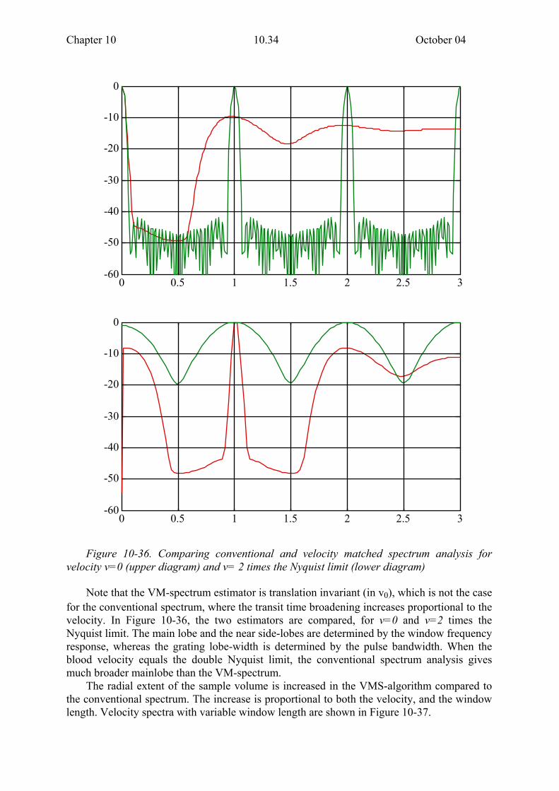
Figure 10-36. Comparing conventional and velocity matched spectrum analysis for
velocity v=0 (upper diagram) and v= 2 times the Nyquist limit (lower diagram) Note that the VM-spectrum estimator is translation invariant (in v0), which is not the case
for the conventional spectrum, where the transit time broadening increases proportional to the velocity. In Figure 10-36, the two estimators are compared, for v=0 and v=2 times the Nyquist limit. The main lobe and the near side-lobes are determined by the window frequency response, whereas the grating lobe-width is determined by the pulse bandwidth. When the blood velocity equals the double Nyquist limit, the conventional spectrum analysis gives much broader mainlobe than the VM-spectrum.
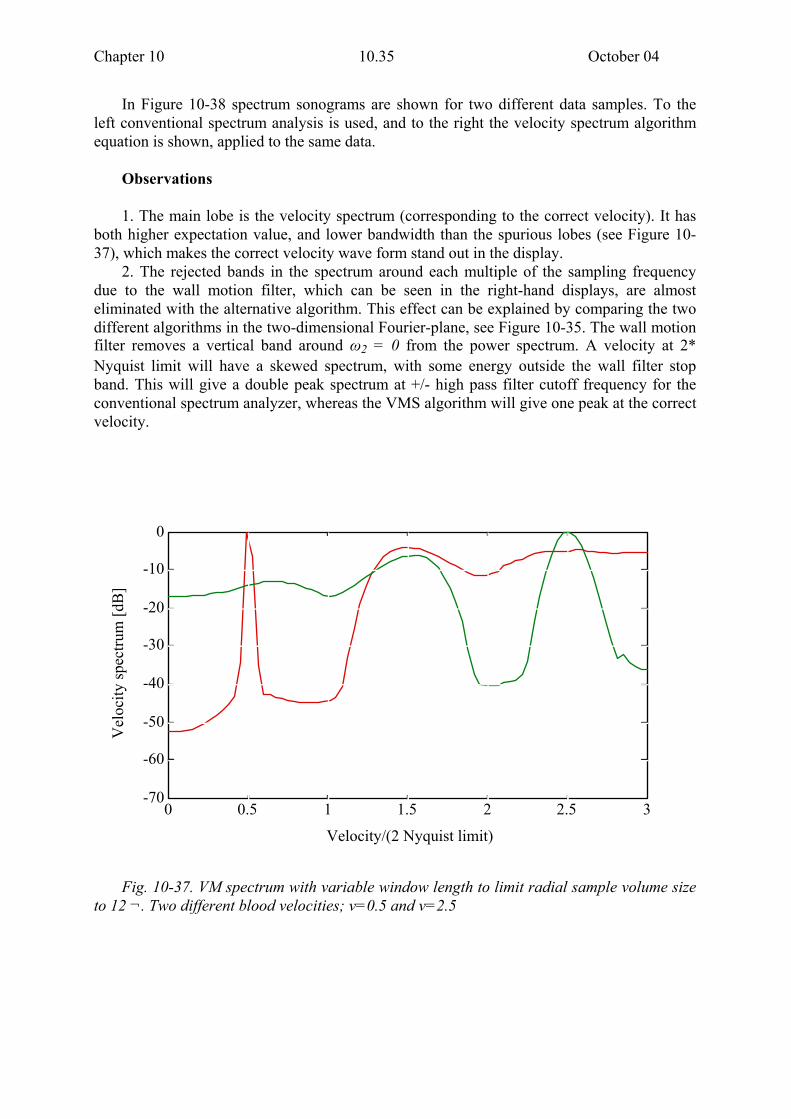
The radial extent of the sample volume is increased in the VMS-algorithm compared to the conventional spectrum. The increase is proportional to both the velocity, and the window length. Velocity spectra with variable window length are shown in Figure 10-37.
Chapter 10 10.35 October 04
In Figure 10-38 spectrum sonograms are shown for two different data samples. To the left conventional spectrum analysis is used, and to the right the velocity spectrum algorithm equation is shown, applied to the same data.
Observations 1. The main lobe is the velocity spectrum (corresponding to the correct velocity). It has
both higher expectation value, and lower bandwidth than the spurious lobes (see Figure 10-37), which makes the correct velocity wave form stand out in the display.
2. The rejected bands in the spectrum around each multiple of the sampling frequency due to the wall motion filter, which can be seen in the right-hand displays, are almost eliminated with the alternative algorithm. This effect can be explained by comparing the two different algorithms in the two-dimensional Fourier-plane, see Figure 10-35. The wall motion filter removes a vertical band around ω2 = 0 from the power spectrum. A velocity at 2* Nyquist limit will have a skewed spectrum, with some energy outside the wall filter stop band. This will give a double peak spectrum at +/- high pass filter cutoff frequency for the conventional spectrum analyzer, whereas the VMS algorithm will give one peak at the correct velocity.
-70
-60
-50
-40
-30
-20
-10
0
0 0.5 1 1.5 2 2.5 3
Velocity/(2 Nyquist limit)
Vel
ocity
spec
trum
[dB
]
Fig. 10-37. VM spectrum with variable window length to limit radial sample volume size
to 12 ¬. Two different blood velocities; v=0.5 and v=2.5

Chapter 10 10.36 October 04
-50
50
-50
50
-100
-50
50
100
-100
-50
50
100
Figure 10-38. VM-spectrum analysis (right) compared to conventional spectrum analysis
(left) applied to signals from human subclavian artery (upper), and aortic artery (lower). 10.7 References
[1] H. L. van Trees, Detection, Estimation, and Modulation theory, Part III: John Wiley & Sons, New York, 1971.
[2] M. B. Priestly, Spectral Analysis and Time Series. London: Academic Press, 1981. [3] K. Kristoffersen, “Real time spectrum analysis in Doppler ultrasound blood velocity measurement,”
SINTEF report Nov. 1984.
[4] H. Torp, “Signal processing in realtime, two dimensional Doppler color flow mapping,” : University of Trondheim, Norway, 1991. [5] H. L. van Trees, Detection, estimation, and modulation theory. Part I,: John Wiley & Sons, New
York, 1968. [6] L. S. Wilson, “Description of Broadband Pulsed Doppler Ultrasonic Processing using the Two-
Dimensional Fourier Transform,” Ultrasonic Imaging, vol. 13, pp. 301 - 315, 1991.

Chapter 10 10.37 October 04
[7] H. Torp, K. Kristoffersen, and B. Angelsen, “Autocorrelation Techniques in Color Flow Imaging. Signal model and statistical properties of the Autocorrelation estimates,” IEEE Trans. on Ultrasonics, Ferroelectrics, and Frequency control, vol. 41, pp. 604 - 612, 1994.
[8] H. Torp and K. Kristoffersen, “Velocity Matched Spectrum Analysis: A new Method for
suppressing Velocity Ambiguity in Doppler Sonogram,” Ultrasound in Medicine and Biology, vol. 21, no. 7, pp. 937 - 944, 1995.
[9] H. Torp, “Clutter rejection filters in Color Flow Imaging: A theoretical Approach,” IEEE Trans. on Ultrasonics, Ferroelectrics, and Frequency control, vol. 44, no. 2, pp. 417 - 424, 1996.
[10] A. Kadi and T. Loupas, “On the performance of Regression and step-initialized IIR Clutter filters for
color Doppler systems in diagnosing medical ultrasound,” IEEE Trans. on Ultrasonics, Ferroelectrics, and Frequency control, vol. 42, no. 5, pp. 927 - 937, 1995.
[11] A. P. Hoeks, J. J. van-de-Vorst, A. Dabekaussen, P. J. Brands, and R. S. Reneman, “An efficient
algorithm to remove low frequency Doppler signals in digital Doppler systems,” Ultrason Imaging, vol. 13, no. 2, pp. 135-44, 1991.