HAL Id: hal-00848841https://hal.archives-ouvertes.fr/hal-00848841

Submitted on 29 Jul 2013

HAL is a multi-disciplinary open accessarchive for the deposit and dissemination of sci-entific research documents, whether they are pub-lished or not. The documents may come fromteaching and research institutions in France orabroad, or from public or private research centers.

L’archive ouverte pluridisciplinaire HAL, estdestinée au dépôt et à la diffusion de documentsscientifiques de niveau recherche, publiés ou non,émanant des établissements d’enseignement et derecherche français ou étrangers, des laboratoirespublics ou privés.

Estimation of 5-min solar global irradiation on tiltedplanes by ANN method in Bouzareah, Algeria

Kahina Dahmani, Gilles Notton, Rabah Dizene, Christophe Paoli, CyrilVoyant, Marie Laure Nivet, Keniouche Karouk

To cite this version:Kahina Dahmani, Gilles Notton, Rabah Dizene, Christophe Paoli, Cyril Voyant, et al.. Estimationof 5-min solar global irradiation on tilted planes by ANN method in Bouzareah, Algeria. Call forPapers The first International Conference on Nanoelectronics, Communications and Renewable Energy(ICNCRE’13), Sep 2013, Algeria. �hal-00848841�

Estimation of 5-min solar global irradiation on tilted

planes by ANN method in Bouzareah, Algeria

K. Dahmani, R. Dizene

Laboratory of Energy Mechanic and Conversion Systems

Science and Technology University Houari Boumédiène

BP 32 El Alia 16111 Bab Ezzouar, Algiers, Algeria

dahmani_kahina@yahoo.fr

G. Notton, C. Paoli, C. Voyant, M.L. Nivet

Laboratory Science for the Environment

University of Corsica, Route des Sanguinaires

F20000 Ajaccio, France

gilles.notton@univ-corse.fr

F. Keniouche

Electromechanical Department, Laboratory of Electro-mechanic

University Badji Mokhtar

Annaba, Algeria

Abstract— Calculation of solar global irradiation on tilted planes

from horizontal global one is difficult when the time step is small.

We used an Artificial Neural Network (ANN) to realize this

conversion at a 5-min time step for solar irradiation data of

Bouzareah (Algeria). The ANN is developed and optimized on the

basis of two years of solar data (1.5 year or training and 0.5 year

for test) and the accuracy of the optimal configuration is around

8% for the nRMSE.

Keywords- Solar irradiation; Artificial Neural Network;

Estimation

I. INTRODUCTION

Monthly average values allow to realize a preliminary sizing, radiation data with a smaller time step are required for performing a more precise sizing or modeling. Commercial softwares for solar systems tilt the horizontal global irradiation contained in their database with generally a low accuracy. So, it would be useless to develop precise models if the tilted input data are too approximated. In this work, we calculate the global irradiation on a 36.8° tilted plane (angle equal to the site latitude) from only horizontal global irradiation collected each 5 minutes using ANN method.

As said by Behr [1], three main reasons make it impossible to develop a simple model for converting horizontal global solar radiation into inclined radiation:

• The radiation incident on a tilted plane includes the radiation reflected by the environment;

• The plane being tilted, only a part of the sky is “seen” and the sky diffuse radiation depends not only on the inclination of the collector, on the sun elevation and azimuth but also on the sky state rarely uniform introducing anisotropic effects difficult to quantify. There are two problems relating to the sky anisotropy: the circum-solar brightness due to the solar radiation diffusion by aerosols concentrated in the sky area around the sun and the horizon brightness near the horizon which is even more important in clear skies;

• measured tilted data are relatively rare in the World.

In the next, we first present briefly the different components of solar radiation. Then, we describe the data used in this work. Next, artificial neural network concepts are detailed. Finally we expose and comment the results obtained and we give some perspectives to conclude this paper.

II. SOLAR RADIATION COMPONENTS

When solar radiation enters the earth’s atmosphere, the incident energy is removed by scattering and absorption. The scattered radiation is called diffuse component. A part goes back to the space and another one reaches the ground directly in line from the solar disk, this part is called beam radiation (Fig. 1).

ββββ

-

sky diffuse

normal beam

beam

ground reflected diffuse

Figure 1. Solar radiation on a tilted surface

The solar radiation arriving on a tilted collector has, most of the time, a beam component (nil by cloudy sky), two diffuse ones coming from the sky and from the ground (Fig. 1.).

III. METEOROLOGICAL STATION AND DATA

The “Centre for Development of Renewable Energies” (CDER) has a meteorological station in Bouzareah near Algiers (latitude: 36.8°N; longitude: 3.17°E) at an altitude of 347 m (Fig. 2). The site is characterized by a Mediterranean climate with dry and hot summers and damp and cool winters.

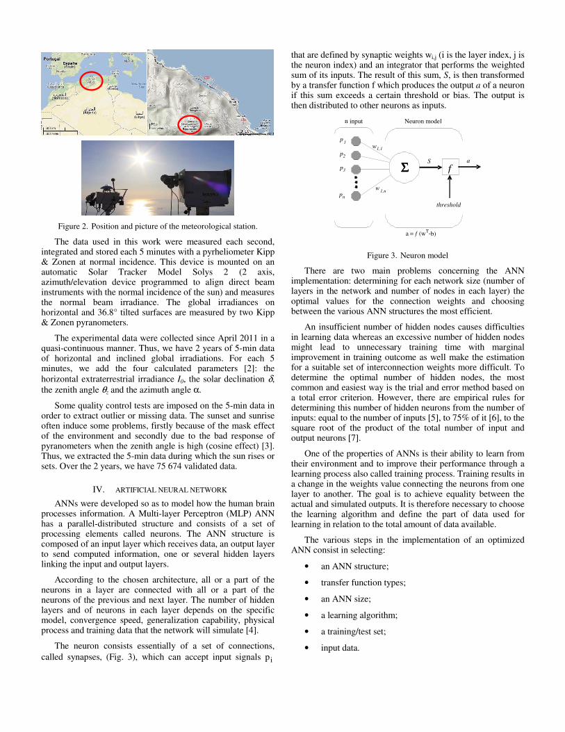
Figure 2. Position and picture of the meteorological station.

The data used in this work were measured each second, integrated and stored each 5 minutes with a pyrheliometer Kipp & Zonen at normal incidence. This device is mounted on an automatic Solar Tracker Model Solys 2 (2 axis, azimuth/elevation device programmed to align direct beam instruments with the normal incidence of the sun) and measures the normal beam irradiance. The global irradiances on horizontal and 36.8° tilted surfaces are measured by two Kipp & Zonen pyranometers.

The experimental data were collected since April 2011 in a quasi-continuous manner. Thus, we have 2 years of 5-min data of horizontal and inclined global irradiations. For each 5 minutes, we add the four calculated parameters [2]: the

horizontal extraterrestrial irradiance I0, the solar declination δ,

the zenith angle θz and the azimuth angle α.

Some quality control tests are imposed on the 5-min data in order to extract outlier or missing data. The sunset and sunrise often induce some problems, firstly because of the mask effect of the environment and secondly due to the bad response of pyranometers when the zenith angle is high (cosine effect) [3]. Thus, we extracted the 5-min data during which the sun rises or sets. Over the 2 years, we have 75 674 validated data.

IV. ARTIFICIAL NEURAL NETWORK

ANNs were developed so as to model how the human brain processes information. A Multi-layer Perceptron (MLP) ANN has a parallel-distributed structure and consists of a set of processing elements called neurons. The ANN structure is composed of an input layer which receives data, an output layer to send computed information, one or several hidden layers linking the input and output layers.

According to the chosen architecture, all or a part of the neurons in a layer are connected with all or a part of the neurons of the previous and next layer. The number of hidden layers and of neurons in each layer depends on the specific model, convergence speed, generalization capability, physical process and training data that the network will simulate [4].

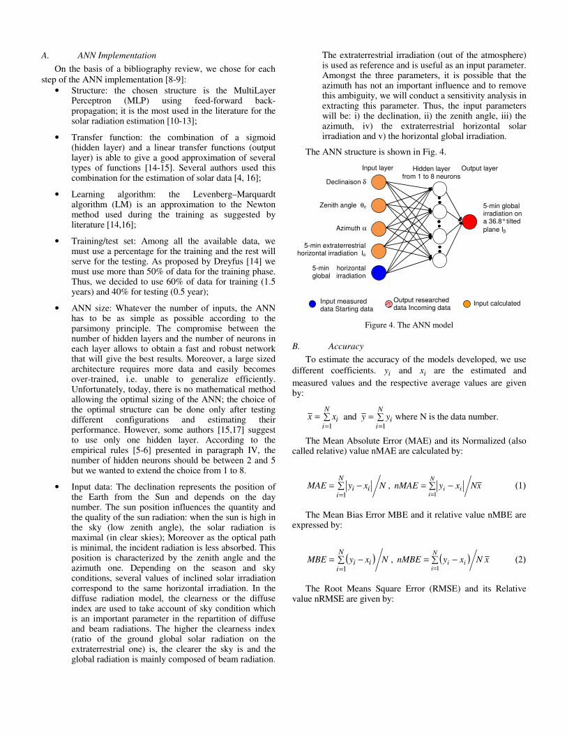
The neuron consists essentially of a set of connections,

called synapses, (Fig. 3), which can accept input signals ip

that are defined by synaptic weights wi,j (i is the layer index, j is the neuron index) and an integrator that performs the weighted sum of its inputs. The result of this sum, S, is then transformed by a transfer function f which produces the output a of a neuron if this sum exceeds a certain threshold or bias. The output is then distributed to other neurons as inputs.

ΣΣΣΣ f

w 1,1

w 1,n

p 1 p 2 p 3

p n

S

a

a =

f ( w

T - b)

threshold

Neuron model

n input

Figure 3. Neuron model

There are two main problems concerning the ANN implementation: determining for each network size (number of layers in the network and number of nodes in each layer) the optimal values for the connection weights and choosing between the various ANN structures the most efficient.

An insufficient number of hidden nodes causes difficulties in learning data whereas an excessive number of hidden nodes might lead to unnecessary training time with marginal improvement in training outcome as well make the estimation for a suitable set of interconnection weights more difficult. To determine the optimal number of hidden nodes, the most common and easiest way is the trial and error method based on a total error criterion. However, there are empirical rules for determining this number of hidden neurons from the number of inputs: equal to the number of inputs [5], to 75% of it [6], to the square root of the product of the total number of input and output neurons [7].

One of the properties of ANNs is their ability to learn from their environment and to improve their performance through a learning process also called training process. Training results in a change in the weights value connecting the neurons from one layer to another. The goal is to achieve equality between the actual and simulated outputs. It is therefore necessary to choose the learning algorithm and define the part of data used for learning in relation to the total amount of data available.

The various steps in the implementation of an optimized ANN consist in selecting:

• an ANN structure;

• transfer function types;

• an ANN size;

• a learning algorithm;

• a training/test set;

• input data.

A. ANN Implementation

On the basis of a bibliography review, we chose for each

step of the ANN implementation [8-9]:

• Structure: the chosen structure is the MultiLayer Perceptron (MLP) using feed-forward back-propagation; it is the most used in the literature for the solar radiation estimation [10-13];

• Transfer function: the combination of a sigmoid (hidden layer) and a linear transfer functions (output layer) is able to give a good approximation of several types of functions [14-15]. Several authors used this combination for the estimation of solar data [4, 16];

• Learning algorithm: the Levenberg–Marquardt algorithm (LM) is an approximation to the Newton method used during the training as suggested by literature [14,16];

• Training/test set: Among all the available data, we must use a percentage for the training and the rest will serve for the testing. As proposed by Dreyfus [14] we must use more than 50% of data for the training phase. Thus, we decided to use 60% of data for training (1.5 years) and 40% for testing (0.5 year);

• ANN size: Whatever the number of inputs, the ANN has to be as simple as possible according to the parsimony principle. The compromise between the number of hidden layers and the number of neurons in each layer allows to obtain a fast and robust network that will give the best results. Moreover, a large sized architecture requires more data and easily becomes over-trained, i.e. unable to generalize efficiently. Unfortunately, today, there is no mathematical method allowing the optimal sizing of the ANN; the choice of the optimal structure can be done only after testing different configurations and estimating their performance. However, some authors [15,17] suggest to use only one hidden layer. According to the empirical rules [5-6] presented in paragraph IV, the number of hidden neurons should be between 2 and 5 but we wanted to extend the choice from 1 to 8.

• Input data: The declination represents the position of the Earth from the Sun and depends on the day number. The sun position influences the quantity and the quality of the sun radiation: when the sun is high in the sky (low zenith angle), the solar radiation is maximal (in clear skies); Moreover as the optical path is minimal, the incident radiation is less absorbed. This position is characterized by the zenith angle and the azimuth one. Depending on the season and sky conditions, several values of inclined solar irradiation correspond to the same horizontal irradiation. In the diffuse radiation model, the clearness or the diffuse index are used to take account of sky condition which is an important parameter in the repartition of diffuse and beam radiations. The higher the clearness index (ratio of the ground global solar radiation on the extraterrestrial one) is, the clearer the sky is and the global radiation is mainly composed of beam radiation.

The extraterrestrial irradiation (out of the atmosphere) is used as reference and is useful as an input parameter. Amongst the three parameters, it is possible that the azimuth has not an important influence and to remove this ambiguity, we will conduct a sensitivity analysis in extracting this parameter. Thus, the input parameters will be: i) the declination, ii) the zenith angle, iii) the azimuth, iv) the extraterrestrial horizontal solar irradiation and v) the horizontal global irradiation.

The ANN structure is shown in Fig. 4.

Input layer Hidden layer from 1 to 8 neurons

Output layer

Declinaison δ

Azimuth α

Zenith angle θz

5-min extraterrestrial horizontal irradiation Io

5-min horizontal global irradiation

5-min global irradiation on a 36.8° tilted

plane Iβ

Input measured data Starting data

Output researched data Incoming data

Input calculated data

Figure 4. The ANN model

B. Accuracy

To estimate the accuracy of the models developed, we use

different coefficients. iy and ix are the estimated and

measured values and the respective average values are given by:

�==

N

iixx

1

and �==

N

iiyy

1

where N is the data number.

The Mean Absolute Error (MAE) and its Normalized (also called relative) value nMAE are calculated by:

NxyMAEN

iii� −=

=1

, xNxynMAEN

iii� −=

=1

(1)

The Mean Bias Error MBE and it relative value nMBE are expressed by:

( ) NxyMBEN

iii� −=

=1

, ( ) xNxynMBEN

iii� −=

=1

(2)

The Root Means Square Error (RMSE) and its Relative value nRMSE are given by:

( ) NxyRMSEN

iii� −=

=1

2

( ) xNxynRMSEN

iii

���

�

���

�� −==1

2 (3)

The Determination Coefficient R² is given by:

( )( )

( ) ( )21

1

2

1

2

12

�A

BCD

��

���

�� −��

���

�� −

��

���

�� −−

=

==

=

N

ii

N

ii

N

iii

xxyy

xxyy

R (4)

V. RESULTS

Our objective is to find the simplest and performant MLP model and to estimate its accuracy. The most commonly used is the feed forward MLP with one hidden layer and one output layer [18-19]. It is often used for modeling and forecasting solar radiation. Several studies [13,20] have validated this approach based on ANN as a non linear model to model solar radiation.

After the input variables for the model are fixed, the next step consists in the determination of the network architecture. The number of inputs and outputs are previously fixed. The choice of the hidden neurons follows a heuristic approach where several networks with different values of the hidden neurons are trained. In this study, we varied this number from 1 to 8 (according to the empirical rules presented in the beginning of paragraph 4) and each MLP architecture was trained 8 times in view to avoid random effects.

In order to test and validate the model, we calculated the

coefficients presented in paragraph IV.B. between measured

and estimated global irradiation on the 36.8° tilted plane. As

we explained in paragraph IV.A, we would like to know if the

azimuth is an input data which improves the model. The

accuracy values for the ANN using respectively five and four

input data (without azimuth) are presented in tables 1 and 2

(calculated on the basis of 8 simulations by architecture). The

first column contains the number of neurons in the hidden

layer.

TABLE I. AVERAGE STATISTICAL TEST BETWEEN MEASURED AND

ESTIMATED GLOBAL SOLAR RADIATION ON A 36.8° TILTED PLANE WITH 5

INPUTS

N MAE nMAE MBE nMBE RMSE nRMSE R²

Wh.m-2 % Wh.m-2 % Wh.m-2 %

1 5.93 16.29 -0.96 -2.65 6.87 18.88 0.977

2 3.03 8.32 -0.26 -0.72 3.87 10.65 0.990

3 2.88 7.92 -0.67 -1.84 3.75 10.30 0.992

4 2.51 6.91 -0.50 -1.37 3.39 9.31 0.993

5 2.43 6.67 -0.56 -1.55 3.23 8.88 0.994

6 2.66 7.30 -0.96 -2.64 3.56 9.77 0.994

7 2.69 7.39 -1.03 -2.84 3.65 10.03 0.993

8 2.62 7.21 -0.96 -2.65 3.61 9.89 0.993

TABLE II. AVERAGE STATISTICAL TEST BETWEEN MEASURED AND

ESTIMATED GLOBAL SOLAR RADIATION ION 36.8 PLANE OPTIMIZED MODEL

WITH 4 INPUTS (WITHOUT AZIMUTH)

N MAE nMAE MBE nMBE RMSE nRMSE R²

Wh.m-2 % Wh.m-2 % Wh.m-2 %

1 5.94 16.32 -0.97 -2.67 6.89 18.93 0.977

2 2.95 8.12 -0.29 -0.80 3.81 10.48 0.991

3 2.80 7.71 -0.50 -1.39 3.65 10.04 0.992

4 2.41 6.63 -0.31 -0.85 3.21 8.81 0.994

5 2.56 7.04 -0.80 -2.20 3.47 9.54 0.994

6 2.75 7.56 -1.14 -3.14 3.77 10.36 0.993

7 2.68 7.38 -1.09 -3.00 3.68 10.12 0.993

8 2.70 7.43 -1.12 -3.09 3.69 10.14 0.993

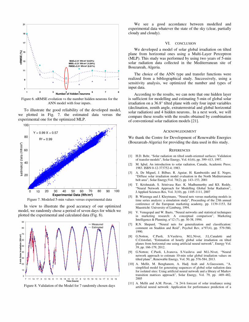
The mean values of the nRMSE and its corresponding

standard deviation were computed and are represented in Figs 5 and 6 for the two models (5 and 4 input neurons) respectively as an error-bar graph. It is observed that the statistical results of both networks show an improvement until reaching the values of 4 hidden neurons, and for higher values of hidden neurons the nRMSE became almost constant and no improvement was observed. In Figs. 5 and 6, the dash points define the 95% confidence interval of the prediction errors (8 simulations), the triangles and square are respectively the minimum and maximum observed errors. We observe the same trend for the variation of the nMAE. The best configuration is encircled in red.

We can conclude that an ANN with one hidden layer composed with 4 neurons presents the best accuracy. If we compare the results obtained with the artificial network using four input neurons or five input neurons, it appears that the use of a fifth input neuron, the sun azimuth, does not provide any significant improvement. Thus, we will retain the use of an ANN with 4 input neurons (declination, zenith angle, extraterrestrial and horizontal irradiations). We must keep in mind that if the average nRMSE for this ANN configuration calculated on 8 simulations is 8.81%, the best simulation with this ANN structure conduced to an nRMSE of 8.27%.

7

9

11

13

15

17

19

21

1 2 3 4 5 6 7 8Number of hidden neurons

nR

MS

E (

%)

MAE=2.51 Wh/m² (6.9%)

MBE=-0.49 Wh/m² (-1.37%)

RMSE=3.39 Wh/m² (9.31%)

Figure 5. nRMSE evolution vs. the number hidden neurons for the

ANN model with five inputs.

7

9

11

13

15

17

19

21

1 2 3 4 5 6 7 8Number of hidden neurons

nR

MS

E (

%)

MAE=2.41 Wh/m² (6.63%)

MBE=-0.31 Wh/m² (-0.84%)

RMSE=3.21 Wh/m² (8.81%)

Figure 6. nRMSE evolution vs the number hidden neurons for the

ANN model with four inputs.

To illustrate the good reliability of the developed model,

we plotted in Fig. 7. the estimated data versus the

experimental one for the optimized MLP.

� �� �� �� �� �� �� �� � A� ����

��

��

��

�

���

BCDEF��E�����������������

B�

���

��E

���

���

����

���

��

�

B������� AA!�BCDEF�"�� ��

#����� AA

�

0 10 20 30 40 50 60 70 80 90 100

20

40

60

80

100

Experimental Data (Wh/m²)

Y = 0.99 X + 0.57

R² = 0.99

Figure 7. Modeled 5-min values versus experimental data

In view to illustrate the good accuracy of our optimized model, we randomly chose a period of seven days for which we plotted the experimental and calculated data (Fig. 8).

0

10

20

30

40

50

60

70

80

90

7 11 14 17 9 13 16 8 11 15 18 10 13 17 9 12 15 19 10 14 17 9 12 16Time (hours)

5-m

in S

ola

r Ir

rad

iati

on

(W

h/m

²)

MeasuredEstimated

Figure 8. Validation of the Model for 7 randomly chosen days

We see a good accordance between modelled and experimental data whatever the state of the sky (clear, partially cloudy and cloudy).

VI. CONCLUSION

We developed a model of solar global irradiation on tilted plane from horizontal ones using a Multi-Layer Perceptron (MLP). This study was performed by using two years of 5-min solar radiation data collected in the Mediterranean site of Bouzareah, Algeria.

The choice of the ANN type and transfer functions were realized from a bibliographical study. Successively, using a sensitivity analysis, we optimized the number and types of input data.

According to the results, we can note that one hidden layer is sufficient for modelling and estimating 5-min of global solar irradiation on a 36.8° tilted plane with only four input variables (declination, zenith angle, extraterrestrial and global horizontal solar radiation) and 4 hidden neurons.. In a next work, we will compare these results with the results obtained by combination of conventional solar radiation models [21].

ACKNOWLEDGMENT

We thank the Centre for Development of Renewable Energies

(Bouzareah-Algeria) for providing the data used in this study.

REFERENCES

[1] H.D. Behr, “Solar radiation on tilted south-oriented surfaces: Validation of transfer-models”, Solar Energy, Vol. 61(6), pp. 399–413, 1997.

[2] M. Iqbal, An introduction to solar radiation, Canada, Academic Press; 1983. ISBN 0-12-373752-4; 1983.

[3] A. De Miguel, J. Bilbao, R. Aguiar, H. Kambezidis and E. Negro, “Diffuse solar irradiation model evaluation in the North Mediterranean belt area”, Solar Energy;Vol. 70(2), pp. 143–153, 2001

[4] T. Krishnaiah, S. Srinivasa Rao. K. Madhumurthy and KS. Reddy, “Neural Network Approach for Modelling Global Solar Radiation”, J.Applied Sciences Res, Vol. 3(10), pp. 1105-1111, 2007

[5] B. Wierenga and J. Kluytmans, “Neural nets versus marketing models in time series analysis: a simulation study”, Proceeding of the 23th annual conference of the European marketing academy, pp. 1139-1153, Ed Maastricht: University of Limburg, 1994.

[6] V. Venugopal and W. Baets, “Neural networks and statistical techniques in marketing research: A conceptual comparison”, Marketing Intelligence & Planning, n°12 (7), pp. 30-38, 1994.

[7] R.N. Shepard, “Neural nets for generalization and classification: comment on Staddon and Reid”, Psychol Rev, n°97(4), pp. 579-580, 1990.

[8] G.Notton, C.Paoli, S.Vasileva, M.L.Nivet, J.L.Canaletti and C.Cristofari, “Estimation of hourly global solar irradiation on tilted planes from horizontal one using artificial neural network”, Energy Vol. 39, pp. 166-179, 2012.

[9] G.Notton; C.Paoli, L.Ivanova, S.Vasileva and M.L.Nivet, “Neural network approach to estimate 10-min solar global irradiation values on tilted plane”, Renewable Energy, Vol. 50, pp. 576-584, 2013.

[10] A. Mellit, M. Benghanem, A. Hadj Arab and A.Guessoum, “A. simplified model for generating sequences of global solar radiation data for isolated sites: Using artificial neural network and a library of Markov transition matrices approach”, Solar Energy, Vol. 79, pp. :469–482, 2005

[11] A. Mellit and A.M. Pavan, .”A 24-h forecast of solar irradiance using artificial neural network: Application for performance prediction of a

grid-connected PV plant at Trieste, Italy”, Solar Energy; Vol. 84, pp. 807–821, 2010.

[12] C. Voyant, M. Muselli, C. Paoli and M.L. Nivet, “Optimization of an artificial neural network dedicated to the multivariate forecasting of daily global radiation”, Energy; Vol. 36(1), pp. 348-359, 2011.

[13] S.A. Kalogirou and A. �encan, ‘Artificial Intelligence Techniques in

Solar Energy Applications’, Theory and Applications, ISBN 978-953-307-142-8, 2010.

[14] G. Dreyfus., J. Martinez, M. Samuelides, M. Gordon, F. Badran and S. Thiria. Apprentissage statistique : Réseaux de neurones - Cartes topologiques - Machines à vecteurs supports, 3 éd. Eyrolles; 2008.

[15] G. Cybenko, ‘ Approximation by superposition of sigmoidal function, Math. Control Signals Systems (1989) 2, 303-314.

[16] K.S. Reddy and R. Manish, “Solar resource estimation using artificial neural networks and comparison with other correlation models”, Energy Conversion and Management; Vol. 44, pp. 2519–2530, 2003.

[17] C. Voyant, Prédiction de series temporelles de rayonnement solaire global et de production d’énergie photovoltaïque à partir de réseaux de neurones artificiels, pHd dissertation, University of Corsica, 16/11/2011.

[18] K. Hornik, M. Stinchcombe and H. White 1989. “Multilayer feedforward networks are universal approximators”, Neural Networks. Vol. 2(5), pp. 359–66, 1989.

[19] Y. Ito, “Representation of functions by superpositions of a step or sigmoid function and their applications to neural network theory”,. Neural Networks, Vol. 4(3), pp. :385–94, 1991

[20] G.P. Zhang and M. Qi, “Neural network forecasting for seasonal and trend time series”, European Journal of Operational Research, Vol. 160(2), pp. 501–514, 2005.

[21] G.Notton, P.Poggi, C.Cristofari, “Predicting hourly solar irradiations on inclined surfaces based on the horizontal measurements: Performances of the association of well-known mathematical models”, Energy Conversion and Management, Vol. 47-13-14, pp. 1816-1829, 2006.