Estimation for Faults Prediction from Component Based Software

ISSN (Print) : 2319-5940 ISSN (Online) : 2278-1021

International Journal of Advanced Research in Computer and Communication Engineering

Vol. 2, Issue 7, July 2013

Copyright to IJARCCE www.ijarcce.com 2630

Estimation for Faults Prediction from

Component Based Software Design using Feed

Forward Neural Networks

Sandeep Kumar Jain1 & Manu Pratap Singh

2

Department of Computer Science

Institute of Engineering & Technology, Dr. B.R. Ambedkar University, Khandari, Agra-282002, India1,2

Abstract: As far as the software system is concerned, the reliability is one of the important quality attributes in

software development process. The recently growing trends in software development process witnessed the paradigm

shift to component based software. The reliability of component based software is difficult to estimate directly by

taking the reliability of individual components into account and measuring the component reliability in software is not

an easy task alike. In this paper we propose a method to estimate the reliability of the software consisting of

components by using different neural network architectures. The proposed method considers software consisting of

components divided into different sets and observes the number of faults encountered over a cumulative execution time

interval for the known set of components and after this we estimate the number of faults predicted for the randomly

chosen set of components in software over next cumulative execution time interval. In this process, we estimate the

faults prediction behavior in the set of components over a cumulative execution time interval besides this the prediction

of faults is estimated for the complete software. We apply the feed forward neural network architectures & its

generalization capability to predict the faults in each component of the software with the prediction of faults for the

complete software for given cumulative execution time.

Keywords: software reliability estimation, component based software reliability, feed forward neural network, fault

prediction.

1. INTRODUCTION:

Component based software reliability estimation is an

emerging and still a trust area of software engineering. The

architecture of software in itself emerges with motivation

for predicting reliable behavior of overall system [1].The

reliability of the component based software reflects the

interdependency with reliability of components. It is one of

the possibilities that overall software system reliability

effects with the functioning of its components. On the

other aspect the overall reliability of the software does not

affect with the failure of any component. The reliability

tolerance limit must specify in this aspect. Software system

design is a high level abstraction of a software system; its

components and their connection. Thus software system

design complements component definition which focuses

on the individual components and their interfaces. The

failure occurrence in any component may cause the failure

in whole software system design, this gives the connection

between components and system design. It is natural to

extend contacts to the level as architectural specification

and worthwhile to develop specialized methods for the

prediction of reliability for component based software

system design [2]. The model of software reliability

prediction for component based software should consider

the nature of fault population contained within the whole

software as well as in the components of software.

Therefore, due to these faults the software exhibits the

failure behavior. It is well defined that the most useful

reliability criteria are residual fault density or the failure

intensity. There are various different

Software reliability growth models have also been

proposed [3, 4, 5]. Every model has its own limitation and

criteria for predicting the reliability of software. As far as

concerns of component based software, the mean time to

failure occurrence will consider for whole software as well

as for each component of the software. These proposed

models are considered to model the failure process and to

characterize how software reliability varies with time and

other factors. These models are used not only to estimate

the current values of the reliability measures such as the

residual fault density, the failure intensity and mean time

to failure but also to predict their future values. It is found

with empirical evidence [6,7] that different models have

different predictive accuracy at different phases of testing

and there is no single analytic model that can be relied on

for accurate prediction in all software . Therefore, the

selection of particular model is very important in software

reliability estimation. The selection of the model can

consider in two ways (i) by generating the applicability of





software reliability growth models by analyzing their

predictability across a broad range of dataset and (ii) by

developing an adaptive model building system [8]. The

problem in first approach is the issue of generalization

which remains partially unanswered due to the lack of

availability of sufficient data sets for software as well as

for its various components. The second approach i.e.

adaptive model, which does not depend on assumed

parameters and based on only the last failure history of the

software system as whole and also failure history of its

each component. The failure history of components of

software produces an immense effect for predicting the

future failures by the software depending on the failure

history and so that the adaptive model should consider the

failure history of complete software system with the failure

history information of each component to predict the

possible future failures by the software. In the literature,

the adaptive model or non-parametric models like neural

network and support vector machine (SVM) based on

statistical failure data such as cumulative failure detected,

failure rate, time between failures, next time to failure etc.

[9, 10]. There are various attempts have been reported in

literature review for using neural network techniques to

model the software reliability prediction. In [11] the first

time neural network is used to predict software reliability.

In this work, feed forward neural network and recurrent

neural networks along with Elman neural network and

Jordan neural network is used for predicting the

cumulative number of detected faults by using execution

time as input. This work also discussed the effects of

various training procedures applied to neural network

namely data representation methods, architectural issues

concluding that neural network can construct models with

varying complexity and adaptability for different datasets

in a realistic environment. In [12] the two methods are

described for software reliability prediction, first neural

networks and second recalibration for parametric models

that were compared by using common predictability

measure and common data sets. The comparative results

revealed that neural network could be used for better trend

prediction. In [13], the effectiveness of the neural back

propagation network method (BPNN) is investigated for

software reliability assignment and prediction using

multiple recent inter failure times as input to predict the

next failure time. In this work the performance of neural

network architecture with various numbers of input nodes,

hidden nodes is evaluated and concluded that the

effectiveness of a neural network method depends on the

nature of data sets up to a larger extent. In [14], a modified

Elnan recurrent neural network is proposed to model and

predict software failure trends. In [15], the artificial neural

network is implemented to software reliability modeling

and examined several conventional software reliability

growth models by eliminating some unrealistic

assumption. In [16], the feed forward back propagation

algorithm is applied to predict the software reliability. In

this work different failure data sets collected from several

standard software projects has been applied to neural

network model. It has also been seen in [17] that the neural

network model is considered as a better estimator for the

software reliability predictor rather than statistical

approaches. In most of the previous works the neural

network is trained with the data sets of past history of

failures in the software for the specific period of time [18,

19, 20]. The trained neural network is expected to predict

the occurrence of failure for the time period which has not

presented in the data sets. Thus, the prediction of software

reliability is depending upon the occurrence of failures in

the given time period used in the training data set. This

approach is working quite effectively for the simple

software system design. The same approach could not

work with so effectively for predicting the reliability of

component based software. Reliability prediction for the

component based software will not only depend upon the

failure history of software but also on the reliability of

each interdependent component. The software reliability

for each component is predicted with occurrence of

failures in the given time period for the component. The

estimated reliability of components is further used to

estimate the reliability of the whole software. Therefore, in

this present work the feed forward neural networks are

used to predict the reliability of component based software.

In this approach a dataset of failure occurrence for each

component in given time period is considered as the local

training set. Thus, each component has its own local

training set. These training sets consist with occurrence of

failure for the component in specific period of same time.

There is feed forward neural network corresponds to each

component. These neural networks are trained with local

training sets of respective components. The prediction of

reliability for each component is considered from

respective trained neural network architecture. Thus, we

have the set of trained neural network corresponds to each

component in the software. The output of these neural

networks and the failure history of the software for a

specific period of time are now used to construct the global

training set for the main neural network which is

predicting the expected failure for the time period not used

in the global training set. Thus, this neural network is used

to estimate the reliability of component based software for

the presented time period. This is obvious that the

prediction of reliability for component software depends

on the reliability state of each component and previous

failure information about the software.

The rest of the paper is organized in four sections. The

section 2 discusses about the multilayer neural network

and back propagation learning rule, section 3 of the paper

presents the simulation and implementation details, section

4 incorporates the results & discussion. Section 5 considers

the conclusion followed by references.

2. Multilayer Feed Forward Neural Network:

The multilayer feed forward neural network can be used to

capture the classification explicitly in the set of input

output pattern collected during an experiment and

simultaneously expected to model the unknown system or





function from which the prediction can be made for the

new or unknown set of data [2]. The collected input-output

pattern pairs are presented to neural network on repeated

basis to accomplish the training of the neural network for

capturing the implicit relation function between input and

output pattern pairs. Once the mapping function between

the input-output pair is captured or estimated the network

can be used to predict the future projection for any

unknown set of input pattern(test pattern set), which has

not been provided during the training. The network

produced the output for this unknown input pattern, this

output will be an interpolated version of the output patterns

corresponding to the input training patterns close to the

given test input pattern. Thus, the network can be used for

the prediction after the effective training or learning. The

neural network architecture requires the training set of

sample examples of input-output pattern pairs to

accomplish the learning. A feed forward neural network

architecture as shown in figure 1 is needed to perform the

task of training.

Figure 1: Feed Forward Multilayer Neural Network Architecture

This neural network consist of differentiable continuous

but non linear output function in all processing units [22]

of output and all hidden layer. The number of processing

units in the input layer corresponds to the dimensionality

of the input pattern vectors are linear. The number of

processing units in the output layer corresponds to the

number of distinct classes in the pattern classification. The

number of processing units in the hidden layers and the

number of hidden layers in the network correspond to the

convex of classes. All the processing units of input layer

are interconnected to all the processing units of the hidden

layers and all the processing units of the hidden layer are

interconnected to the processing units of the output layer

and weight is associated with each connection. We can use

supervised leaning method i.e generalized delta learning

rule so that a network can be trained to capture the

mapping explicitly in the set of input output pattern

collected during an experiment and simultaneously

expected to model the unknown system or function from

which the prediction can be made for the new or unknown

set of data not used in the training set [23]. The possible

output pattern class would be approximately an

interpolated version of the output pattern class

corresponding to the input learning pattern close to the

given test input pattern. This method involves the

modification of the weight between the processing units of

successive layers. For such an updating of weight in the

supervisory mode, it becomes necessary to know the

desired output for each unit in the hidden and output layers

so that the instantaneous squared error (the difference

between the desired and actual output for the current

presented input pattern from each unit of the output layer)

may be used to guide the updating of the weights. We

propagate the error from output layers to successive hidden

layers for updating the weights. This leaning method is

known as back-propagation learning [24, 25] based on the

principle of gradient descent along the error surface in

weight space. In this proposed neural network architecture

the activation value and output values of the units of

output layer and hidden layer are shown with following set

of equations.

The activation and output signal for the jth

units of output layer for the presented input pattern at the kth

iteration can

represent as:

𝑦𝑗𝑘 = 𝑆ℎ 𝑞ℎ

𝑘 𝑊𝑗ℎ (2.1)

𝐻

ℎ=1





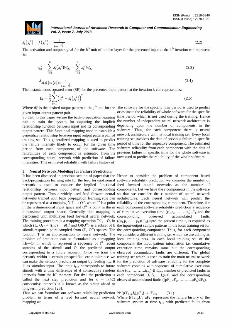
𝑆𝑗 𝑦𝑗ℎ = 𝑓 𝑦𝑗

ℎ =1

1+𝑒−𝑦𝑗

𝑘 (2.2)

The activation and output signal for the hth

unit of hidden layer for the presented input at the kth

iteration can represent

as:

𝑞ℎ𝑘 = 𝑆𝑖 𝑥𝑖

ℎ 𝑊ℎ𝑖

𝑛

𝑖=1

= 𝑥𝑖𝑘 𝑊ℎ𝑖

𝑛

𝑖=1

(2.3)

𝑆ℎ 𝑞ℎ

𝑖 =𝑓 𝑞ℎ𝑘 =

1

1+𝑒−𝑞ℎ

𝑘

(2.4)

The instantaneous squared error (SE) for the presented input pattern at the iteration k can represent as:

𝐸𝑘 =1

2 𝑑𝑗

𝑘 − 𝑆𝑗 𝑦𝑗𝑘

2

(2.5)

𝑛

𝑗=1

Where 𝑑𝑗𝑘 is the desired output pattern at the j

th unit for the

given input-output pattern pair.

So that, in this paper we use the back-propagation learning

rule to train the system for capturing the implicit

relationship function between input and its corresponding

output pattern. This functional mapping used to establish a

generalize relationship between input output pattern pair of

training set. This generalized mapping is used to predict

the failure intensity likely to occur for the given time

period from each component of the software. The

reliabilities of each component is estimated from its

corresponding neural network with prediction of failure

intensities. This estimated reliability with failure history of

the software for the specific time period is used to predict

or estimate the reliability of whole software for the specific

time period which is not used during the training. Hence

the number of independent neural network architecture is

depending upon the number of components in the

software. Thus, for each component there is neural

network architecture with its local training set. Every local

training set involves the data of previous failure in specific

period of time for the respective component. The estimated

software reliability from each component with the data of

previous failure in specific time for the whole software is

now used to predict the reliability of the whole software.

3. Neural Network Modeling for Failure Prediction:

It has been discussed in previous section of paper that the

back-propagation learning rule for the feed forward neural

network is used to capture the implied functional

relationship between input pattern and corresponding

output pattern. Thus a widely used feed forward neural

networks trained with back propagation learning rule can

be represented as a mapping N:In → O

m, where I

n is a point

in the n dimensional input space and Om is point in the m

dimensional output space. Generally this mapping is

performed with multilayer feed forward neural network.

The training procedure is a mapping operation T:Ik→Ok in

which (Ik, Ok) = {(i,o) ⃓ i∈In and O∈O

m} is a subset of k

stimuli-response pairs sampled from (In, O

m) spaces. The

function T is an approximation to neural network. The

problem of prediction can be formulated as a mapping

f:Il→Ol in which Il represent a sequence of Ith

recent

samples of the stimuli and Ol the predicted output

corresponding to a future moment. Once we train the

network within a certain prespecified error tolerance we

can make the network predicts an output by feeding ik+d ∈

In as stimulus input. The input ik+d corresponds to future

stimuli with a time difference of d consecutive random

intervals from the kth

moment. For d=1 the prediction is

called the next step prediction and for d = n(≥2)

consecutive intervals it is known as the n-step ahead or

long term prediction [26].

Hence to consider the problem of component based

software reliability prediction we consider the number of

feed forward neural networks as the number of

components. Let we have the r components in the software

so that we consider the r number of neural network

architectures. Each neural network will predict the

reliability of the corresponding component. Therefore, for

each component software reliability prediction a sequence

of cumulative execution time ((t1,t2,………tk)∈Tk and the

corresponding observed accumulated faults

((μ1,μ2,……μk)∈Fk) upto the present time tk is required as

the input-output sample patterns in the local training set for

the corresponding component. Thus, for each component

we consider a different training set which we are calling as

local training sets. In each local training set of the

component, the input pattern information i.e. cumulative

execution time remains same but the corresponding

observed accumulated faults are different. The global

training set which is used to train the main neural network

for the prediction of software reliability for the complete

software contains with sequence of cumulative execution

time (tk+1,……….tk+q) ∈ Tn+q, number of predicted faults in

each component (f1,f2,…..fr)∈Fr and the corresponding

observed accumulated faults ((μF1,μF2,………..μFn)∈Fk).

Thus we can formulate our software reliability prediction

problem in terms of a feed forward neural network

mapping as:

N:{((Tk+q,fr),μFk}→μFk+h (3.1)

Where ((Tk+q,fr), μFk) represents the failure history of the

software system at time tk+q with predicted faults from





each component at time tk used to train the network and

μFk+h the network’s prediction. Similarly, we can also

formulate the software reliability prediction problem for

each component in terms of local feed forward neural

network mapping as:

𝑁𝑟 : { 𝑇𝑘 , 𝐹𝑘 𝑟 , 𝑡𝑘+ℎ} → 𝜇𝑘+ℎ𝑟 (3.2)

Where 𝑇𝑘 , 𝐹𝑘 𝑟 represents the failure history of rth

component of the system at time tk used to train the rth

network and 𝜇𝑘+ℎ𝑟 the r

th network prediction for the r

th

component of the software. Thus, on the successful

training of neural network, it can be used to predict the

total number of faults to be detected at the end of a future

test session k+h feeding tk+h as its input. In the process of

training, the two techniques are used to exhibit the

predictive capability of neural network. The first method is

used in the generalization training. This is the standard

way in which most of the feed forward neural networks are

trained. During training, each input it at time t is associated

with the corresponding output Ot. Here, the network learns

to generalize the actual functionality between the input

variable and the output variable. The second regime is

used in the prediction training. It refers to an approach

used in training recurrent networks. Under this training the

value of the input variable it at time t is associated with the

value of the output variable Ot+1 corresponds to the next

time step t+1. Here the network learns to predict output

anticipated at the next time step rather than computing

outputs corresponding to the present input [27].

Hence for the prediction or estimation for the expected

number of faults, we consider a component based software

for which we are interested in estimating the reliability.

Let the software consists of r individual components. Each

component has cumulative execution time and its own

accumulated faults. Therefore, we consider the r different

neural network architecture. Now we consider the arbitrary

rth

component from the components of software. The rth

component considers the 𝑡1𝑟 , 𝑡2

𝑟 , ………………𝑡𝑘𝑟

cumulative execution times and 𝑓1𝑟 , 𝑓2

𝑟 , ……… . . 𝑓𝑘𝑟 are

observed accumulated faults. This set of execution time

and accumulated faults consider the training set of the rth

component and in such a way each component has its own

training set. Thus at any instant of time we have the r local

training sets. Therefore individual r neural networks are

trained with corresponding local training set and predict

the expected number of faults in the next instant of

execution time. Hence the training set for rth

component is

represented as:

𝑇𝑟 = 𝑡1

𝑟 , 𝑓1𝑟 , 𝑡2

𝑟 , 𝑓2𝑟 , ………………… . . 𝑡𝑛

𝑟 , 𝑓𝑟𝑛 (3.3)

The rth

neural network is initialized with random weights

prior to learning. In the process of learning for input-

output pattern pairs of training set Tr, patterns are

presented on repeated basis. Suppose an arbitrary input

pattern 𝑡𝑙𝑟 is presented at iteration m on the current values

of weights. The neural network nr produces the output

pattern:

𝑁𝑟 = {𝑆1(𝑦1𝑟 𝑙 ,𝑆2 𝑦2

𝑟 𝑙 , . . 𝑆𝑗 𝑦𝑗𝑟 𝑙 …𝑆𝑝 𝑦𝑝

𝑟 𝑙 (3.4)

Suppose number of units in the output layer is P so that the

instantaneous square error at lth

iteration is defined as:

𝐸𝑙𝑟 =

1

2 (𝑓𝑙

𝑟 − 𝑆𝑗 𝑦𝑗𝑟 𝑙

2𝑃

𝑗=1

(3.5)

The weights will converge to optimal weights by

modification in the weights during the training process of

network for capturing the required mapping function. The

training process is in such a way that the weight changes at

current iteration will proportional to the gradient descent

along the instantaneous error surface i.e.

∆𝑊𝑗ℎ 𝑙 = −𝜂0

𝜕𝐸𝑙𝑟

𝜕𝑊𝑗ℎ(𝑙) 𝑓𝑜𝑟 𝑜𝑢𝑡𝑝𝑢𝑡 𝑙𝑎𝑦𝑒𝑟 (3.6)

And ∆𝑊ℎ𝑖 𝑙 = −𝜂ℎ𝜕𝐸𝑙

𝑟

𝜕𝑊ℎ𝑖(𝑙) 𝑓𝑜𝑟 ℎ𝑖𝑑𝑑𝑒𝑛 𝑙𝑎𝑦𝑒𝑟 (3.7)

Hence with the chain rule in limit of stochastic gradient method we have: 𝜕𝐸𝑙

𝑟

𝜕𝑊𝑗ℎ(𝑙)

= 𝜕𝐸𝑙

𝑟

𝜕𝑦𝑗𝑟(𝑙)

.𝜕𝑦𝑖

𝑟(𝑙)

𝜕𝑊𝑖ℎ(𝑙)

=𝜕𝐸𝑙

𝑟

𝜕𝑦𝑗𝑟 𝑙

. 𝑆ℎ(𝑞ℎ𝑟 𝑙 )

or

𝜕𝐸𝑙𝑟

𝜕𝑊𝑖ℎ(𝑙)

=𝜕𝐸𝑙

𝑟

𝜕𝑆𝑗 (𝑦𝑗𝑟 𝑙 )

.𝜕𝑆𝑗 (𝑦𝑗

𝑟 𝑙 )


. 𝑆ℎ(𝑞ℎ𝑟 𝑙 )

= ∆𝑙𝑟 . 𝑆ℎ(𝑞ℎ

𝑟 𝑙 (3.8)

Where ∆𝑙𝑟=

𝜕𝐸𝑙𝑟

𝜕𝑆𝑗 (𝑦𝑗𝑟(𝑙)

.𝜕𝑆𝑗 (𝑦𝑗

𝑟(𝑙)


Now, ∆𝑙𝑟=

𝜕𝐸𝑙𝑟

𝜕𝑆𝑗 (𝑦𝑗𝑟(𝑙)

. 𝑆𝑗 (𝑦𝑗𝑟 𝑙 )(1 − 𝑆𝑗 𝑦𝑗

𝑟 𝑙 )

= − 𝑓𝑗𝑙𝑟 − 𝑆𝑗 𝑦𝑗

𝑟 𝑙 𝑆𝑗 𝑦𝑗𝑟 𝑙 (1 − 𝑆𝑗 (𝑦𝑗

𝑟 𝑙 )𝑝𝑗=1 )

So that from equation (3.6) we have

∆𝑊𝑗ℎ 𝑙 = 𝜂0∆𝑙𝑟 . 𝑆ℎ 𝑞ℎ

𝑟 𝑙 (3.9)

And 𝑊𝑗ℎ 𝑙 + 1 = 𝑊𝑗ℎ 𝑙 + 𝜂0∆𝑙𝑟𝑆ℎ 𝑞ℎ

𝑟 𝑙 (3.10)

Similarly, from equation (3.7) we have 𝜕𝐸𝑙

𝑟

𝜕𝑊ℎ𝑖(𝑙)=

𝜕𝐸𝑙𝑟

𝜕𝑞ℎ𝑟(𝑙)

.𝜕𝑞ℎ

𝑟(𝑙)

𝜕𝑊ℎ𝑖(𝑙)





= 𝜕𝐸𝑙

𝑟

𝜕𝑞ℎ𝑟 𝑙

. 𝑡𝑘𝑟 𝑙

= 𝜕𝐸𝑙

𝑟

𝜕𝑆ℎ (𝑞ℎ𝑟(𝑙)

.𝜕𝑆ℎ(𝑞ℎ

𝑟(𝑙)

𝜕𝑞ℎ𝑟 𝑙

. 𝑡𝑘𝑟(𝑙)

= 𝜕𝐸𝑙

𝑟

𝜕𝑆ℎ 𝑞ℎ𝑟 𝑙

. 𝑆ℎ 𝑞ℎ𝑟 𝑙 1 − 𝑆ℎ 𝑞ℎ

𝑟 𝑙 . 𝑡𝑘𝑟(𝑙)

= 𝜕𝐸𝑙

𝑟

𝜕𝑦𝑗𝑟 .

𝜕𝑦𝑗𝑟 𝑙

𝜕𝑆ℎ(𝑞ℎ𝑟(𝑙)

. 𝑆ℎ(𝑞ℎ𝑟 𝑙 )(1 − 𝑆ℎ 𝑞ℎ

𝑟 𝑙 . 𝑡𝑘𝑟(𝑙)

= ∆𝑙𝑟 . 𝑊𝑗ℎ . 𝑆ℎ 𝑞ℎ

𝑟 𝑙 (1 − 𝑆ℎ 𝑞ℎ𝑟 𝑙 ) . 𝑡𝑘

𝑟(𝑙)

Therefore, from equation (3.7) we have

∆𝑊ℎ𝑖 𝑙 = 𝜂ℎ∆𝑙𝑟 . 𝑊𝑗ℎ . 𝑆ℎ 𝑞ℎ

𝑟 𝑙 1 − 𝑆ℎ 𝑞ℎ𝑟 𝑙 . 𝑡𝑘

𝑟 𝑙 (3.11)

and

𝑊ℎ𝑖 𝑙 + 1 = 𝑊ℎ𝑖 𝑙 + 𝜂ℎ∆𝑙𝑟 . 𝑊𝑗ℎ. 𝑆ℎ 𝑞ℎ

𝑟 𝑙 1 − 𝑆ℎ 𝑞ℎ𝑟 𝑙 . 𝑡𝑘

𝑟 𝑙 (3.12)

Hence in this way all the neural networks i.e. l to r are

combined for the learning process with their local training

sets. Thus, these r neural networks are able to predict

reliability of each components in generalize way.

After this, we consider our global training set to

accomplish the training of main neural network

architecture for the prediction of software reliability for the

complete software. This training set consists of sequence

of cumulative execution time i.e. (tk+1, tk+2,……………tk+q

∈ Tk), the number of possible predicted faults in each

component and the corresponding observed accumulated

faults (μF1, μF2,………….. μFn) ∈ Fn from the whole

software i.e.

𝐺𝑇 = { 𝑡𝑘+1, 𝑓1𝑘+1, ……𝑓𝑟

𝑘+1 , 𝜇𝐹𝑘+1 ,

(𝑡𝑘+2, 𝑓1𝑘+2 … . . 𝑓𝑟

𝑘+2 , 𝜇𝐹𝑘+2 … . . 𝑡𝑘+𝑞 𝑓1𝑘+𝑞

. . , 𝑓𝑟𝑘+𝑞

, 𝜇𝐹𝑘+𝑞} (3.13)

Now this training is presented to neural network

architecture which is predicting the reliability of the whole

software. This prediction depends upon number of failures

in cumulative execution time and predicted faults in each

component. During the training process the weight update

in neural network architecture for output and hidden layer

can define in similar manner of equation (3.10) and (3.11).

Hence we have:

∆𝑊ℎ𝑖 𝑙 = 𝜂ℎ∆𝑙𝑊𝑗ℎ . 𝑆ℎ 𝑞ℎ 𝑙 1

− 𝑆ℎ 𝑞ℎ 𝑙 . 𝑥𝑖𝑙 (3.14)

and 𝑊ℎ𝑗ℎ 𝑙 = 𝜂0∆𝑙𝑆ℎ 𝑞ℎ 𝑙 (3.15)

where

∆𝑙 = − 𝜇𝐹𝑗𝑘+𝑙 − 𝑆𝑗 𝑦𝑗

𝑙 . 𝑆𝑗 (𝑦𝑗𝑙)(1 − 𝑆𝑗 𝑦𝑗

𝑙 )

𝑝

𝑗=1

⩝ 𝑑

= 1 𝑡𝑜 𝑞

and

𝑥𝑖𝑙 = 𝑡𝑘+𝑑

𝑖 + 𝑓𝑖𝑗𝑘+𝑑

𝑟

𝑗=1

⩝ 𝑖 = 1 𝑡𝑜 𝑛 𝑎𝑛𝑑 𝑑

= 1 𝑡𝑜 𝑞 (3.16) Thus, the set of neural network i.e. r in number are used to

predict failures in the presented time as input pattern

through the captured implied function relationships by the

network. This predicted information is used with

cumulative execution time to predict the reliability of

whole software. Therefore, it is now required to consider

the formation of local training sets and global training set

with proper encoding for cumulative execution time and

accumulated faults to accomplish the implementation and

simulation of proposed method.

4. Implementation Detail and Simulation Design:

In this section of implementation detail and simulation

design we consider the input-output pattern representation

for training with the selection of various required

parameters & architecture to accomplish the training for

prediction of reliability in component based software. So

that before we attempt to use neural network it is necessary

to encode the patterns in a form that is suitable for the

training pattern to the neural network. As we know that the

neuron state variable in feed forward networks is restricted

to 0 to 1.0 or -1.0 to +1.0 due to the sigmoid single

function use in the units of hidden and output layers.

Hence the input/output variables of the problem should be

encoded to conform to this range. It is obvious that for

prediction problem where input/output variable may range

over a large numerical value and to use the direct binary

encoding is a trivial form. However, such a direct scaling

may result both in the lost of prediction accuracy and the

network failure to discriminate different output values.

Some of such schemes are found in literature [28] to

address this situation. A better generalization and

prediction is obtained [6,7] using gray coding when

compared to binary encoding representation. Thus the

gray coding is used to eliminate hamming clifts in the

input representation. Thus in our application we employ a





simple gray code representation because our data set

represents a sequence of increasing numerical values and

prediction is near this kind of hamming clift resulted in

very high error and this anomaly reduced with the use of

Gray coding. Therefore, in order to simulate the

experiment for the prediction of reliability in component

based software model, we have combined the individual

neural network architecture for each component with its

local training set. The global training set for the neural

network which is used to predict the reliability for whole

software includes extra values in terms of predicted faults

from the components of software. Therefore the number of

units used in the input and the output layer is determined

by the number of bits used to encode the input and the

output variables used in our experiments for the

components in the software and for the complete software.

Tables from 1.1 to 1.10 are showing the encoding used for

the components and their corresponding observed faults.

Table 1.1: Coding for 1st software(SW1) containing 10 components with faults

Time Number of

Components

Faults Detected Input Encoding Output Encoding

t1-t5 4+3+3 3+5+6 000000.0110.0010.0010 00010.00111.00101

t6-t10 4+3+3 2+4+5 000001.0110.0010.0010 00011.00110.00111

t11-t15 4+3+3 2+3+8 000010.0110.0010.0010 00011.00010.01100

t16-t20 4+3+3 0+4+4 000011.0110.0010.0010 00000.00110.00110

t21-t25 4+3+3 1+2+1 000110.0110.0010.0010 00001.00011.00001

Table 1.2: Coding for 2nd

software(SW2) containing 20 components with faults

Time Number of

Components

Faults

Detected

Input Encoding Output Encoding

t1-t5 8+5+7 14+6+9 000000.1100.0111.0100 01001.00101.01101

t6-t10 8+5+7 11+8+8 000001.1100.0111.0100 01110.01100.01100

t11-t15 8+5+7 6+6+6 000011.1100.0111.0100 00101.00101.00101

t16-t20 8+5+7 8+4+3 000010.1100.0111.0100 01100.00110.00100

t21-t25 8+5+7 5+2+1 000110.1100.0111.0100 00111.00011.00001

Table 1.3: Coding for 3rd

software(SW3) containing 30 components with faults.

Time Number of

Components

Faults

Detected


t1-t5 7+14+9 11+20+9 000000.0100.1001.1101 01110.11110.01101

t6-t10 7+14+9 8+22+7 000001.0100.1001.1101 01100.11101.00100

t11-t15 7+14+9 5+17+10 000011.0100.1001.1101 00111.11001.01111

t16-t20 7+14+9 7+11+6 000010.0100.1001.1101 00100.01110.00101

t21-t25 7+14+9 4+9+2 000110.0100.1001.1101 00110.01101.00011

Table 1.4: Coding for 4th


Time Number of

Components

Faults

Detected


t1-t5 4+3+2 14+7+8 000000.0110.0010.0011 01001.00100.0110

t6-t10 4+3+2 11+8+9 000001.0110.0010.0011 01110.01100.01101

t11-t15 4+3+2 6+6+9 000011.0110.0010.0011 00101.00101.01101

t16-t20 4+3+2 7+4+8 000010. 0110.0010.0011 00100.00110.01100

t21-t25 4+3+2 1+5+2 000110. 0110.0010.0011 00001.00111.00011


software(SW5) containing 25 components with faults.

Time Number of

Components

Faults

Detected


t1-t5 8+10+7 11+9+20 000000.1100.1111.0100 01110.01101.11110

t6-t10 8+10+7 6+11+8 000001. 1100.1111.0100 00101.01110.01100

t11-t15 8+10+7 2+4+9 000011. 1100.1111.0100 00011.00110.01101

t16-t20 8+10+7 17+10+5 000010. 1100.1111.0100 11001.01111.00111

t21-t25 8+10+7 7+22+8 000110. 1100.1111.0100 00100.11101.01100







Time Number of

Components

Faults

Detected


t1-t5 5+4+3 15+11+12 000000.0111.0110.0010 01000.01110.01010

t6-t10 5+4+3 12+15+11 000001.0111.0110.0010 01010.01000.01110

t11-t15 5+4+3 15+18+0 000011.0111.0110.0010 01000.11011.00000

t16-t20 5+4+3 1+8+16 000010.0111.0110.0010 00001.01100.11000

t21-t25 5+4+3 16+15+3 000110.0111.0110.0010 11000.01000.00010



Time Number of

Components

Faults

Detected


t1-t5 10+8+6 6+5+4 000000.1111.1100.0101 00101.00111.00110

t6-t10 10+8+6 5+4+1 000001.1111.1100.0101 00111.00110.00001

t11-t15 10+8+6 15+14+13 000011.1111.1100.0101 01000.01001.01011

t16-t20 10+8+6 13+15+5 000010.1111.1100.0101 01001.01000.00111

t21-t25 10+8+6 5+6+19 000110.1111.1100.0101 00111.00101.11010



Time Number of

Components

Faults

Detected


t1-t5 11+12+14 0+9+12 000000.1110.1010.1001 00000.01101.01010

t6-t10 11+12+14 14+11+4 000001.1110.1010.1001 01001.01110.00110

t11-t15 11+12+14 9+8+8 000011.1110.1010.1001 01101.01100.00100

t16-t20 11+12+14 3+3+9 000010.1110.1010.1001 00010.00100.01101

t21-t25 11+12+14 10+11+12 000110.1110.1010.1001 01111.01110.01010



Time Number of

Components

Faults

Detected


t1-t5 3+2+8 12+13+14 000000.0010.0011.1100 01010.01011.01001

t6-t10 3+2+8 6+7+8 000001.0010.0011.1100 00101.00100.01100

t11-t15 3+2+8 9+10+16 000011.0010.0011.1100 01101.01111.11000

t16-t20 3+2+8 9+10+11 000010.0010.0011.1100 01101.01111.01110

t21-t25 3+2+8 2+7+1 000110.0010.0011.1100 00011.00100.00001



Time Number of

Components

Faults

Detected


t1-t5 5+6+7 4+5+6 000000.0111.0101.0100 00110.00111.00101

t6-t10 5+6+7 7+4+2 000001.0111.0101.0100 00100.00110.00011

t11-t15 5+6+7 11+14+9 000011.0111.0101.0100 01110.01001.01101

t16-t20 5+6+7 16+9+5 000010. 0111.0101.010 11000.01101.00111

t21-t25 5+6+7 8+6+7 000110.0111.0101.0100 01100.00101.00100

The number of units used in the neural network for complete software in the input and output layer is determined by the

number of bits used to encode one input for execution time & number of bits to express predicted faults from each

component and the output variables as the number of total actual faults in the complete software in presented

cumulative execution time. Table 2.1 to 2.10 shows the encoding used in our experiments for the complete software.

Table 2.1: Detected faults in cumulative execution time for software(S/W1)

Time No. of Components in

Software one

Faults

Detected


t1-t5 10 31 000000.001111 010000

t6-t10 10 20 000001.001111 011110

t11-t15 10 37 000011.001111 110111

t16-t20 10 28 000010. 001111 010010

t21-t25 10 15 000110. 001111 001000







Software two

Faults

Detected


t1-t5 20 38 000000.011110 110101

t6-t10 20 36 000001.011110 110110

t11-t15 20 30 000011.011110 010001

t16-t20 20 24 000010.011110 011101

t21-t25 20 08 000110.011110 001100



Software three

Faults

Detected Input Encoding Output Encoding

t1-t5 25 15 000000.010101 001000

t6-t10 25 11 000001.010101 001110

t11-t15 25 17 000011.010101 011001

t16-t20 25 14 000010.010101 001001

t21-t25 25 08 000110.010101 001100


Time No. of Components in a

whole Software four

Faults

Detected


t1-t5 30 39 000000.010001 110100

t6-t10 30 47 000001.010001 111000

t11-t15 30 39 000011.010001 110100

t16-t20 30 29 000010.010001 010011

t21-t25 30 17 000110.010001 011001



Software five

Faults


t1-t5 35 18 000000.110010 011011

t6-t10 35 17 000001.110010 011001

t11-t15 35 20 000011.110010 011110

t16-t20 35 22 000010.110010 011101

t21-t25 35 10 000110.110010 001111



Software six

Faults


t1-t5 40 28 000000.111100 010010

t6-t10 40 25 000001.111100 010101

t11-t15 40 28 000011.111100 010010

t16-t20 40 30 000010.111100 010001

t21-t25 40 20 000110.111100 011110



Software seven

Faults


t1-t5 45 28 000000.111011 010010

t6-t10 45 32 000001.111011 110000

t11-t15 45 22 000011.111011 010010

t16-t20 45 15 000010.111011 010001

t21-t25 45 08 000110.111011 011110







Software eight

Faults


t1-t5 50 35 000000.101011 110010

t6-t10 50 40 000001.101011 111100

t11-t15 50 32 000011.101011 110000

t16-t20 50 30 000010.101011 010001

t21-t25 50 28 000110.101011 010010



Software nine

Faults


t1-t5 55 32 000000.101100 110000

t6-t10 55 28 000001.101100 010010

t11-t15 55 25 000011.101100 010101

t16-t20 55 24 000010.101100 011101

t21-t25 55 20 000110.101100 011110



Software ten

Faults


t1-t5 60 44 000000.100010 111010

t6-t10 60 40 000001.100010 111101

t11-t15 60 38 000011.100010 110101

t16-t20 60 32 000010.100010 110000

t21-t25 60 28 000110.100010 010010

Since for each prediction we have the two experiments one

for the components and the other one for the complete

software. As far as first experiment is concerned we

consider the cumulative execution time as a free variable

and the corresponding cumulative faults count as the

dependent variable. Therefore, we trained the network for

components with the execution time as the input and

observed fault count as the target output. It is considered

that the training ensemble at time 𝑡𝑘𝑖 consists of complete

failure history of the ith

component since t=0. As the feed

forward neural network cannot predict well without any

exposure to the failure history of the component, we

imposed a limit on the minimum size of the training

ensemble. Thus in our first experiment the minimum

ensemble size was restricted to 3 data points i.e. the

components are assumed to be at first 3 sessions of test are

over. Hence after successful training for each neural

network with failure history up to 𝑡𝑘1, we fed the future

cumulative time as test input patterns i.e. 𝑡𝑘+1𝑖 to the

neural network of ith

component to get the predicted

number of faults. These predictions are observed up to tq.

Now we consider our second experiment. In this we

trained the neural network with the cumulative execution

time tk+1 to tk+q and predicted faults of components from

first experiment as the input and the observed faults count

from the complete software as the target output. Hence,

after successful training to the network with failure history

up to tk+q and predicted faults from each component up to

tk+q, we fed the network with future cumulative execution

time as input patterns from tk+q+1 to tk+q+u to get the

network’s prediction. Single hidden layer is considered

with 10 neurons for the neural network architecture used

for the components and two hidden layers with 10 and 5

neurons in each is considered for the neural network used

to predict faults from complete software. These selection

are based on the heuristic criteria, which indicates that the

number of inputs are more in global training set with

respect to local training sets. Therefore, the problem of

mapping in complete software is much complex with

respect to the problem of mapping for neural networks of

components. The number of units in hidden layers is

selected as per the suitability of effective performance of

neural network as good generalization and approximation.

5. RESULTS AND DISCUSSION

In our experiment, we consider the different neural

network architectures for predicting the faults in future

cumulative execution time as a free variable. The first

architecture consists of 18 input units, one hidden layer

with ten neurons and one output layer with 15 units. The

second neural architecture is used for predicting the

number of faults for whole software consists of 10 units

and 5 units in hidden layer and one output layer with 6

units. We conducted the whole simulation in two phases

for two different situations. In first phase, we consider the

components for ten different software consisting of

different number of components. In this simulation, we

consider the cumulative execution time as a free variable

for each of the software, the number of components in the

software and corresponding cumulative faults count for

each component of the software as the dependent variable.





We have trained the neural network with the execution

time, components as input after encoding these inputs in

Gray code as input pattern vector of size 18x1. The

observed faults count for each component are considered

as output pattern vector of size 12x1 after encoding of

observed faults in Gray code. In this training, the input

patterns are provided in cumulative time interval from t1-

t25 with the step of five and this training is continued for

each of the software and training graphs for epochs of

convergence are shown from figure 5.1 to figure 5.10.

Figure 5.1

Figure 5.2





Figure 5.3

Figure 5.4





Figure 5.5

Figure 5.6





Figure 5.7

Figure 5.8





Figure 5.9

Figure 5.10





After this the second phase of first experiment was started

for the prediction of detected faults in next cumulative

execution time interval. Here the next cumulative

execution time interval means that the time which is not

being used in our training set. Thus to predict the faults we

consider the cumulative execution time interval from t26-

t50. The trained neural network considered this unknown

next cumulative execution time interval with the number

of components as input pattern vector for simulation. The

simulation behavior of trained neural network is exhibiting

the predicted faults. These predictions of faults for

different software are shown in the figures from 5.11(a) to

5.15(a). These figures 5.11(a) to 5.15(a) are representing

the graphs for number of faults observed in the

components for software in given cumulative execution

time interval whereas figures 5.11(b) to 5.15(b) are

representing the number of predicted faults in components

in the software for future cumulative execution time

interval.

Figure 5.11(a)

Figure 5.11(b)

0

5

10

15

20

25

30

35

No

. o

f

Fau

lts

Dte

tcte

d

No. of faults detected in the components at different time interval

(t1-t25)

0

5

10

15

20

25

No

. of

Pre

dic

ted

Fau

lts

No. of faults predicted in the components at different time

intervals (t26-t50)





Figure 5.12(a)

Figure 5.12(b)

0

5

10

15

20

25

30

No

. of

Fau

lts

Dte

tcte

dNo. of faults detected in the components at different time inteval

(t1-t25)

0

2

4

6

8

10

12

14

16

No

. of

Pre

dci

ted

Fau

lts


inteval (t26-t50)





Figure 5.13(a)

Figure 5.13(b)

0

5

10

15

20

25

30N

o. o

f F

ault

s o

f D

ete

cte

dNo. of faults detected in the components at different time interval

(t1-t25)

0

2

4

6

8

10

12

14

16

No

. o

f Fa

ult

s P

red

icte

d


interval (t26-t50)





Figure 5.14(a)

Figure 5.14(b)

0

5

10

15

20

25

30N

o.

of

Fau

lts

Dte

cte

d

No. of faults detected in the components at different time

interval(t1-t25)

0

2

4

6

8

10

12

14

16

No

. of

Fau

lts

Pre

dic

ted

No. of faults predicted in the components at different time interval

(t26-t50)





Figure 5.15(a)

Figure 5.15(b)

In the analysis of the results it can be seen that the

behavior of faults prediction is a generalized

approximation of the observed faults. Thus it shows that

the predicted faults are approximately tends to interpolated

from observed faults in given cumulative execution time

interval. Now, the first phase of the second experiment is

started in the same manner as previous experiment with the

change that in place of components, the dependent

Variable i.e. observed faults are considered for complete

software in the same cumulative execution time interval.

Here in this experiment the input pattern vector of 12x1 is

presented to the neural network with 6x1 pattern vector as

target output for training. The training is accomplished for

each of the software on same cumulative execution time

interval as it used for its components. The performance of

neural network for complete software is shown in the

figure 5.16 to figure 5.25.

0

5

10

15

20

25

30

35N

o. o

f F

ault

s D

ete

cte

d

No. of faults detected in the components at different time interval

(t1-t25)

0

2

4

6

8

10

12

14

16

No

. of

Fau

lts

Pre

dic

ted


interval (t26-t50)





Figure 5.16

Figure 5.17





Figure 5.18

Figure 5.19





Figure 5.20

Figure 5.21





Figure 5.22

Figure 5.23





Figure 5.24

Figure 5.25





After this training the neural network is simulated for

predicting the number of faults in next cumulative

execution time interval. Thus for evaluating the

performance of trained neural network, we consider the

next cumulative execution time interval t26-t50. The

simulated behavior of the neural network exhibited the

number of detected faults as it can be seen from figure

5.26 to figure 5.35. The graph of figure 5.26 to figure 5.30

are representing the no. of observed faults for given

cumulative execution time interval whereas the graph of

figure 5.31 to figure 5.35 are representing the number of

predicted faults in whole software for unknown next

cumulative execution time interval.

Figure 5.26

Figure 5.27

0

5

10

15

20

25

No

. of

fau

lts

de

tect

ed

No. of Faults Detected in the whole Software at different time

interval (t1-t25)

0

5

10

15

20

25

No

. of

fau

lts

de

tect

ed

No. of Faults Detected in whole Software at different time

interval (t1-t25)





Figure 5.28

Figure 5.29

0

5

10

15

20

25N

o. o

f f

ault

s d

ete

cte

dNo. of Faults Detected in whole Software at different time

interval (t1-t25)

0

5

10

15

20

25

30

No

. of

fau

lts

de

tect

ed


interval (t1-t25)

0

5

10

15

20

25

30

35

No

. of

fau

lts

de

tect

ed


interval (t1-t25)





Figure 5.30

Figure 5.31

Figure 5.32

0

5

10

15

20

25

30

35

No

. of

fau

lts

pre

dic

ted

No. of Faults Predicted in whole Software at different time interval

(t26-t50)

0

5

10

15

20

25

30

35

No

. of

fau

lts

pre

dic

ted

No. of Faults Predicted for whole Software at different time

interval (t26-t50)





Figure 5.33

Figure 5.34

0

5

10

15

20

25

30

35

No. of Faults Predicted in whole Software at different time

interval (t26-t50)

0

5

10

15

20

25

30

35


interval (t26-t50)





Figure 5.35

The graph of predicted faults for each of the software is

same, but it is representing the generalized approximations

of corresponding graphs of number of detected faults in

that software. The characteristics of predicted faults for

each of the software is consistent, it means the prediction

of faults for the software is not behaving in the same

manner as the prediction of faults for the components.

Thus the behavior for predicting the faults in the software

indicates the prediction is independent from the fault

prediction of the components of the software. This

observation concretes the concepts that the software

reliability of software may not depend upon the behavior

of components.

6. CONCLUSION

We know that the software reliability is effective technique

for measurement of software quality over a time period. In

this paper, we employed the feed forward neural

architecture for estimating the reliability of component

based software. This estimation of reliability is considered

in two phases. The first phase included the prediction of

faults in each component of the software for cumulative

execution time. In second phase the faults were predicted

for the complete software. Two stages of feed forward

neural network architecture were used. The first stage of

neural networks architecture is used to predict the faults

from each component. There is as much neural network

architecture as the number of components in the software.

The predictions of faults were based on the generalized

behavior of trained neural network for given training sets.

The final neural network architecture is used for the

prediction of faults from the complete software. This

neural network architecture used the predicted faults from

components as input with cumulative execution time to

estimate the number of predicted faults. The following

observations are drawn from the simulation of proposed

method.

(i) We have considered the software consisting of

components divided into different sets and observed the

number of faults encountered over a cumulative execution

time interval separately for the known set of components.

After that, we estimated the number of faults predicted for

the randomly chosen set of components in software over

next cumulative execution time interval. On comparing the

detected faults and predicted faults, we have found a

generalized faults prediction behavior or a expected

number of faults in the set of components over a

cumulative execution time interval and this can be useful

in estimating the reliability for the set of components over

a next cumulative execution time interval.

(ii) Secondly, we have applied the neural network

architecture for the software as a whole. In case of

complete software, we have observed the number of faults

detected by assuming all the components in the software as

a single unit over cumulative execution time interval. After

that, we observed the predicted number of faults in

randomly chosen software consisting of components over

the next cumulative execution time interval. In doing so,

we have noticed very little variation in number of

predicted faults for randomly chosen different software of

small size over next cumulative execution time interval.

We can conclude that with the help of proposed method

we may estimate the software reliability for the small size

software very effectively as a result of properly trained

neural network architecture and observe a very little

variation in the pattern of number of estimated faults in the

software as single unit of number of components.

(iii) There is an interesting behavior is observed

during the simulation. The predicted faults from the

complete software were approximately same in given

cumulative execution time. This behavior was not found

for their components. Thus, the predicted faults for

cumulative execution time from each component were

different. It indicates that the number of predicted faults

from the complete software may approximately

independent from the predicted number of faults from the

component. Therefore, it is not necessary that if

0

5

10

15

20

25

30

35


interval (t26-t50)





components of software are predicting more number of

faults than the complete software will also consider the

increased number of faults. It is observed from the

simulation of our proposed method that the number of

predicted faults of complete software does not increase

with increased predicted faults of its component. Thus,

estimation of faults for complete software may not depend

upon the estimation of faults prediction from its

components.

In the future, we can extend and explore the pattern of

behavior of number of detected faults and predicted faults

to estimating the software reliability for the software

consisting of tightly interdependent and a very large

number of components.

REFERENCES[1] P.N Mishra: “Software reliability analysis models”, IBM System Journal, pp. 262-270, 22(1983).

[2] Jung Hua Lo, Chin Yu Hung, Sy. Yeh Kuo and M.R. Lyu:

“Sensitivity analysis of software reliability for component based software application”, Proceedings of 27th Annual International Computer

Software and Application Conference, pp. 500-505, 2003.

[3] A.L.Goel: “Software reliability models: Assumptions, Limitations and Applicability”, IEEE Transactions on Software

Engineering, SE11(12), pp. 1411-1423, 1985. [4] J.D.Musa, A.Lannino and K.Okumoto: “Software Reliability:

Measurement, Prediction, Applications”, McGraw Hill, 1987.

[5] S. Brocklehurst, P.Y. Chan, B.Littlewoood and J.Snell: Recalibrating software reliability models”, IEEE Trans. on Software

Engineering, pp. 458-470, 16(1990).

[6] Y.K.Malaiya, N.Karunanithiand P.Verma: “Predictability measures for software reliability models”, proceedings of 14th IEEE

International Computer Software Applications Conference, pp. 7-12,

1990. [7] Y.K. Malaiya, N.Karunanithi and P.Verma: “Predictability of

software reliability models”, Technical Report CS-91-117, Computer

Science Department, Colorado State University, Fort Collins, CO80J23, 1991.

[8] S. Aliahdali and M.Habib: “Software reliability analysis using

parametric and non-parametric methods”, Proceedings of the ISCA, 18th International Conference on Computers and their Application, pp. 63-66,

2003.

[9] Y.Tamura, S.Yamada and M.Kimura: “A software reliability assessment method based on neural networks for distributed development

environment”, Electronics and Communication in Japan, Part 3, 86(11),

pp.13-20, 2003. [10] Y.S.Su and C.Y.Huang: “ Neural Network based apparatus for

software reliability estimation using dynamic weighted combinational

models”, The Journal of Systems and Software, 80(4), pp.606-615, 2007. [11] N.Karunanithi, D.Whitley and Y.K.Malaiya: “Prediction of

software reliability using connectionist models”, IEEE Transaction on

Software Engineering 18(7), pp. 563-574, 1992. [12] R.Sitte: “Comparison of software reliability growth

predictions: neural networks vs. parametric recalibration”, IEEE

Transactions on Reliability 48(3), pp. 285-291, 1999. [13] K.Y.Cai, L.Cai, W.D.Wang, Z.Y.Yu and D.Zhang: “ On the

neural network approach in software reliability modeling”, The Journal of

Systems and Software, vol.58, pp. 47-62, 2001.

[14] S.L.Ho, M.Xie and T.N.Goh: “ A study of the connectionist models for software reliability prediction, Computers and Mathematics

with Applications, vol.46, pp. 1037-1045, 2003.

[15] Jung-Hua Lo” The implementation of artificial neural networks applying to software reliability modeling, Chinese Control and

Decision Confrence (CCDC 2009), 2009.

[16] Y.Singh and P.Kumar: “Prediction of software reliability using feed forward neural networks”, International Conference on

Computational Intelligence and Software Engineering(CiSE), ISBN: 978-1-4244-5391-7, pp.1-5, 2010.

[17] S.H.Aljahdali, K.A.Buragga: “Employing four ANNs

paradigms for software reliability prediction: an Analytical Study”, ICGST-AIML Journal. vol. 8, Issue II, pp.1-8, 2008.

[18] Q.Hu, M.Xie, S.Ng: “Software reliability predictions using

artificial neural networks, Computational Intelligence in Reliability Engineering (SCI) 40, pp. 197-222, 2007.

[19] T.Liang, N.Afzel: “Evolutionary neural network modeling for

software cumulative failure time prediction”, Journal of Reliability Engineering and System Safety, vol.87, pp.45-51, 2005.

[20] N.Gupta and M.P.Singh: “estimation of software reliability

with execution time model using the pattern mapping technique of artificial neural network”, Computer and Operations Research vol.32,

pp.187-199, 2005.

[21] Simon Haykin: “Neural networks and learning machines”, Third Edition, PHI, 2010 .

[22] S.N.Sivanadam, Sumathi, Deepa: “Introduction to neural

networks using Matlab 6.0, Computer Engg. Series TMH, 2010. [23] D.Whitley and N.Karunanithi: “Improving generalization in

feed forward neural networks, Proceedings of the IJCNN, Seattle,WA,

vol.II, pp. 77-82, 1991. [24] P.J.Werbos: “Pattern recognition: New tools for the prediction

and analysis in the behavioral sciences”, Ph.D. thesis, Harvard

University, Cambridge, 1974. [25] D.R. Hush and Horne: “Progress in supervised neural

networks”, IEEE Signal Processing Magazine, vol.10(1), pp.8-39, 1993.

[26] N.Karunanithi and D.Whitley: “Prediction of software reliability using feed forward and recurrent neural nets”, International

Joint Conference on Neural Networks (IJCNN), ISBN: 0-7803-0559-

0/92, vol.1, pp.800-805, 1992. [27] M.I.Jordan: “Attractor dynamics and parallelism in a

connectionist sequential machine, Proceedings of the 8th Annual

Conference of the Cognitive Science, pp.531-546, 1986. [28] M.Ohba: “Software reliability analysis models, IBM Journal

of Research Development, vol.28, pp.428-443, 1984.

Estimation for Faults Prediction from Component Based Software

Documents

Transcript of Estimation for Faults Prediction from Component Based Software