The Journat of Financial Research • Vol. XII, No. 2 • Summer 1989

ESTIMATION AND SELECTION BIAS IN MEAN-VARIANCEPORTFOLIO SELECTION

George M. Frankfurter, Christopher G. LamoureuxLouisiana State University

Abstract

Much research has focused on the problem of selecting portfolios without the benefit ofparametric measures of risk and return. In this paper, a Monte Carlo technique is used toisolate the extent and nature of the problems introduced by this practice. The technique isemployed in the context of classical statistical methodology without permitting short sales. Itis shown that using estimators of expected return and risk not only obscures parametric val-ues, but also affects portfolio composition in the Markowttz framework. In this study, thesetwo components of bias are isolated and measured.

I. Introduction

In this paper, the uncertainty in portfolio selection that arises because of imper-fect knowledge of the return distributions of risky assets is examined. This risk may bedecomposed into two parts: (a) estimation risk; and (b) selection risk. This decompo-sition makes studying the nature and source of bias in portfolio expected return andrisk possible. Further, it is established that some general and ad hoc rules of portfoliodiversification can be useful until the normative model of portfolio selection is restruc-tured. Evidence is provided of the inferiority of widely popularized rules of diversifica-tion based on normative implications of positive models of asset pricing.

II. Literature Review

Any application of Normative Portfolio Theory' (NPT) involves using estimates ofboth return and risk, while the original models of Markowitz and Sharpe assumeknowledge of the first two moments of the ex-ante return distributions. In practicalapplications, decision makers do not have access to these parameters. According tostatistical theory, estimates of the nondecision (or input) variables of the Markowitzportfolio selection procedure are drawn from a distribution, with the true (but un-known) parameters as their respective means.

Kalymon [13], Barry [2], Brown [4, 5], and Alexander and Resnick [1] employBayesian methods to resolve the problem of "estimation risk." Kalymon ([13], p. 560)characterizes estimation risk as a second component of risk: "the decision maker'slack of perfect information about the parameters of his model." In general, the Bay-esian School treats the problem by using predictive distributions. Through application

'NPT refers to the normative model of portfolio selection of Markowitz [16, 17], its simplification bySharpe |18|, and to other works that develop models to deal with normative portfolio decision making.Market equilibrium conditions are not assumed, nor are the normative implications of equilibrium-basedmodels considered.

773

174 The Journai of Financiai Research

of these distributions the need for parameter estimates vanishes. Frost and Savarino((10], p. 303) use a simulation methodology to obtain the resuit that an " 'all stocksare identical" informative prior selects portfolios whose ex-ante performance is supe-rior to that provided by either the Classical Estimated or the Bayes Diffuse investmentrules."

Barry [2i, Brown [4], Jobson and Korkie [Ul, and Klein and Bawa [14) examinethe effect of estimation risk on the CAPM. For instance, Jobson and Korkie [1U de-rive statistical properties of the parameters (e.g., portfolio mean, variance, andweights) in the presence of an orthogonal portfolio, where short selling is unrestricted.Sharpe calls this formulation the "parametric solution," where portfolio weights aredependent on two parameters. In this context, a direct solution of the estimation prob-lem can be found. Unfortunately, no such solution exists under the formulation withnon-negativity constraints on portfolio weights, since portfolio weights cannot be de-rived as a linear combination of a set of parameters.

Thus, a heuristic approach is taken in this paper. In the framework of a MonteCarlo simulation, an understanding is developed of the interactive effects of the selec-tion algorithm's preferences and nominal values of risk-return characteristics.^ Thisinteraction may induce changes in portfolio composition for small changes in inputvariables (the vector of means and the variance-covariance matrix in the case of theMarkowitz algorithm; alpha, beta, and error variance in the case of the Sharpe [18]simplification of Markowitz). The result of this change in composition may be a majordeparture from efficiency in parameter space (if the parameters were known) vis-a-vissample space (when estimates are used).^

The contribution of this paper is the separation of estimation bias from selectionbias. Through this separation, portfolio managers are better able to gauge portfoliorisk-return characteristics, and finance theorists obtain a better understanding of nor-mative portfolio theory.

In the Monte Carlo experiment here, the Sharpe [ 18] diagonal model is the focus.Frankfurter, Phillips, and Seagle [9] show that the simplified diagonal model tends toperform as well as, or better than, the full variance-covariance model in the presenceof limited sample data. Jorion [121 shows that in a full variance-covariance portfolioselection framework, using a Stein-type shrinkage estimator leads to superior portfolioselection. Since the single-index model is used here, the shrinkage estimators and or-dinary least squares estimators are isomorphic.

'Frankfurter, Phillips, and Seagle | 8 | show that straight-forward application of the Markowitz-Sharpealgorithm will overstate return and understate risk.

'The nature of the sensitivity of the portfolio selection algorithm is not addressed directly in this re-search, although the size of selection bias (as defined herein) is positively related to the sensitivity of thealgorithm to perturbations in the inputs. Best and Grauer [31 perform sensitivity analysis in the full vari-ance-CQvariance context.

Estimation and Seiection Bias 175

III. Methodology and Data

Description

In the Monte Carlo experiment here, an environment is simulated in which assetrates of return are generated by a Gaussian process. Portfolio managers operate underthe assumption that the true return-generating process is arithmetic Brownianmotion.

To make the simulation relevant, "true" parameters come from estimates ob-tained with actual data, representing long histories. Monthly NYSE and AMEXCRSP tapes for the period ending December 31, 1985 are used to obtain monthly rateof return data for companies that have two hundred contiguous observations. Accord-ingly, monthly rates of return are obtained for 680 NYSE stocks and 123 AMEXstocks. Input variables required for the Sharpe model are generated from these data toobtain the parameters of the experiment here.

The CRSP equally weighted NYSE index serves as the common factor in Sharpe'ssingle-index model to obtain OLS estimates. These data are used to estimate:

«,, = a, + ^ , « , , + e,, (1)

Here, R,, and R^, represent observed (arithmetic) rates of return, in month t (f =1 , 2 , . . . , 200) for the stock and index, respectively. OLS estimates of a,, )3,, anda (̂f,), along with the index mean and variance constitute the parameters of the MonteCarlo experiment. The two key underlying assumptions of the simulation methodologyare as follows:

1. Stocks inter-relate with each other solely through their respective "covari-ances" with the index.

2. The process is stationary.

In this experiment, therefore, neither lack of stationarity, nor incorrect specificationof the single-index model can be a source of bias.

Each iteration of the experiment represents a random sample of sixty observa-tions on the index and on each of the 803 stocks. From the index of "parametric"values (mean and variance), a sample of sixty observations on the index is obtained.GGNML (from IMSL) is used to generate the standard unit normal values. Next, fromthe parametric value of the error variance for each stock, a sample error is generated.These two values (e,, and R^,), together with the 803 sets of a, and ^i ("parametric")values, are used to obtain the "sample" observations:

R^ir = Ci,-^0iK, + 4 (2)

j = \,2, . . .500

/ = 1, 2, . . . 803

f = 1,2, . . .60

176 The Journal of Financiai Research

where R'i, and /C , are rates of return on stock i and the index, respectively, in simula-tion j ; a; and |3, are parameters; and e{, is a random error in simulation y for stock /.Thus 500 X 804 X 60 (24,120,000) unique observations are generated.

Next, for each simulation ,/. the sixty observations are used to estimate orl. 3^a^tiV, and EiR'J and o\R,^)' (the mean and variance of the index for iteration./) asinputs to the Sharpe simplified model for portfolio selection. Thus, five hundred effi-cient frontiers (EFs) are obtained. Since each of the five hundred EFs represents aconvex set that may map anywhere in mean-standard deviation space, meaningfulcomparisons require additional theoretical motivation.•"

Evaluation

In this research, portfolios are compared according to their shadow prices in pa-rameter space. This approach is used because corner portfolios are unique selectionsof stocks that totally describe the efficient set, as linear combinations of these cornerportfolios provide the entire (continuous) efficient frontier. The shadow price has thefollowing interpretation: the marginal gain, in terms of portfolio expected return,which can be attained by a marginal relaxation of the risk constraint. It also provides asingular measure of preference for a decision maker.

The shadow price of each corner portfolio in parameter space is 9^. Since 114unique corner portfolios are found in parameter space, p = 1,2. . . , 114.^ The highere j is, the more risk averse the investor is. Confronted with a particular EF, an investorwill select a portfolio based on 9? (i.e., a reflection of his risk-return preference).Assuming homothetic preferences, an investor will select portfolios, across EFs, withthe same 9 values. Exploitation of 9 in this fashion affords the most general compari-sons, in the context of the model. This model is theoretically valid for any expectedutility function that depends only on the first two moments of end-of-period wealth.The use of 9^, then, for comparison purposes isolates a particular agent's choice-independent of his utility function—when confronted with different choice variables.

BiasesFor the sake of analysis, it is possible to decompose total bias (defined below) into

two distinct components. One component is estimation bias. This bias is inescapable,and it results from one's having to make inferences about parameters with limitedsample data. The other component is selection bias, a result of portfolio weights beingdependent upon sample-estimated values. This bias would not exist with a naive selec-

^Five hundred simulations are adequate, as all statistics of interest (e.g., standard deviation of biases)become asymptotic after four hundred simulations.

KJnly 55 of the 803 stocks (6.85 percent) enter any of the 114 unique corner portfolios, selected fromactual market data. There is no constraint on the number of corner portfolios in each simulation. This isalso a function of the estimates. Comparing corner portfolios with common shadow prices vitiates any prob-lems that otherwise might arise because of the different nature of the 501 EFs.

Estimation and Selection Bias 177

tion rule.*" Thus, the existence of selection bias, vis-a-vis the naive portfolio buildingrule, may explain the reluctance of portfolio managers and financial theorists to em-brace NPT.

In parameter space, corner portfolios represent risk-return combinations thatresult from multiplying parametric weights by parametric values. These portfolios areunbiased, and thus, truly efficient. In practical application, a decision maker, work-ing with sample values, determines sample weights. Thus, each sample EF is a prod-uct of the respective sample weights and estimated values.

Total bias is the difference between what the investor believes the (sample)optimal portfolio parameters are, and the parameters of portfolios that would be se-lected if all parametric values were known. That is, total bias is the difference: (PW XPV) - (SW X SV), where PW, PV, SW, and SV stand for parametric weights, para-metric values, sample weights, and sample values, respectively. Estimation bias is thatpart of bias that is the difference between a particular portfolio's (indexed by p) para-metric values and the sample estimators of these parameters:

E.B.^ = iSW X PV) - iSW X SV) (3)

Similarly, seiection bias isolates the bias that arises from using sample estimators toselect optimal portfolios.

S.B.p = iPW X PV) - iSW X PV) (4)

It is easy to verify that

iPW X PV)- iSW X 5V) = [iSW X PV) - iSW X SV)] +

[iPW X PV)- iSW X PV)\ (5)

That is.

Total Bias = Estimation Bias + Selection Bias

IV. Results

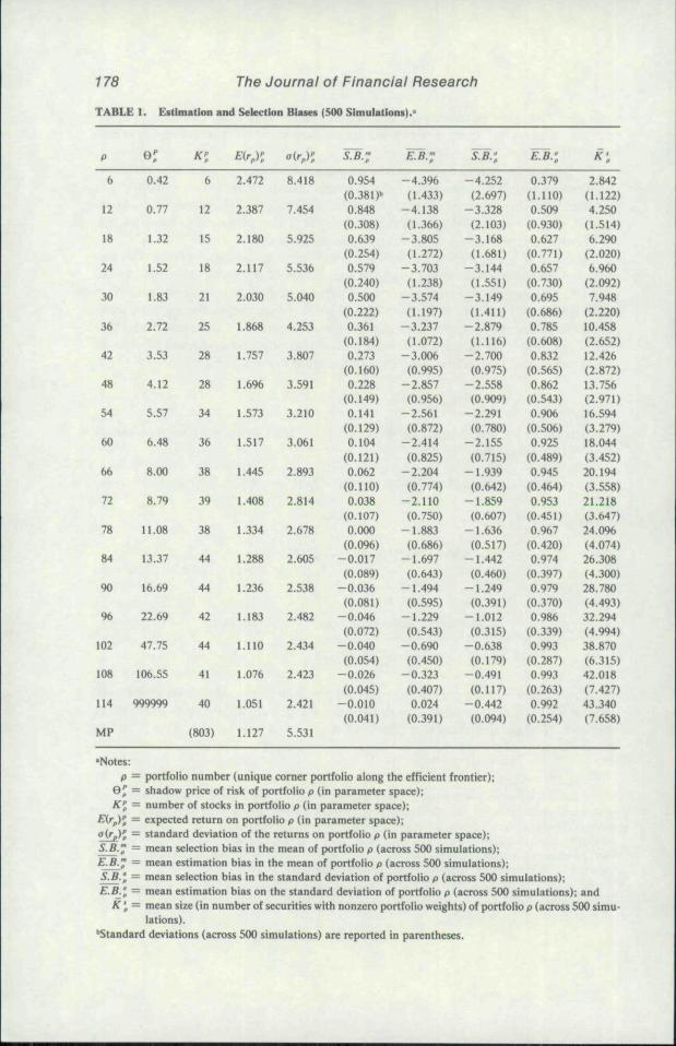
Table 1 provides the parametric expected portfolio return, Eirp)p, standard devi-ation, oirp)p. Op. and the number of securities in a portfolio, A ,̂ for every sixth cornerportfolio.^ The parametric corner portfolios are indexed by p (p = 1, 2, . . . , 114).

'•A common norm is to select 16 securities at random. If one accepts the implications (although not allof the assumptions) of the CAPM, then this strategy would be optimal in the sense of no portfolio exposureto diversifiable risk. Such a portfolio will still have estimation bias. If the market does, in fact, conform lothe CAPM, then il would be expected that in many simulations virtually all of the 803 stocks would enter atleast one efficient portfolio. This is not the case. "Naive" is used to imply a random selection process. In theliterature, the most commonly used naive selection method is equal weighting.

'In the interest of economy, only every sixth corner portfolio is shown in Table 1. The authors willprovide a full list of all corner portfolio values upon request.

178 The Journai of Financiai ResearchTABLE 1. Estimation and Selection Biases (500 Simulations).'

p

6

12

18

24

30

36

42

48

54

60

66

72

78

84

90

96

102

108

114

MP

0.42

0.77

1.32

1.S2

1.83

2.72

3.53

4.12

5.57

6.48

8.00

8.79

11.08

13.37

16.69

22.69

47.75

106.55

999999

ATS

6

12

15

18

21

25

28

28

34

36

38

39

38

44

44

42

44

41

40

(803)

E(rX2.472

2.387

2.180

2.117

2.030

1.868

1.757

1.696

1.573

1.517

1.445

1.408

1.334

1.288

1.236

1.183

1.110

1.076

1.051

1.127

8.418

7.454

5.925

5.536

5.040

4.253

3.807

3.591

3.210

3.061

2.893

2.814

2.678

2.605

2.538

2.482

2.434

2.423

2.421

5.531

S.B.:

0.954(0.381 )f'0.848(0.308)0.639(0.254)0.579(0.240)0.500(0.222)0.361(0.184)0.273(0.160)0.228(0.149)0.141(0.129)0.104(0.121)0.062(0.110)0.038(0.107)0.000(0.0%)-0.017(0.089)

-0.036(0.081)

-0.046(0.072)

-0.040(0.054)-0.026

(0.045)-0.010(0.041)

E.B-

-4.396(1.433)

-4.138(1.366)

-3.805(1.272)

-3.703(1.238)

-3.574(1.197)-3.237

(1.072)-3.006(0.995)

-2.857(0.956)-2.561(0.872)

-2.414

(0.825)-2.204(0.774)

-2.110(0.750)

-1.883(0.686)

-1.697(0.643)-1.494(0.595)

-1.229(0.543)-0.690(0.450)

-0.323(0.407)0.024(0.391)

SB.;

-4.252(2.697)

-3.328(2.103)-3.168(1.681)

-3.144(1.551)-3.149(1.411)

-2.879(1.116)-2.700(0.975)-2.558(0.909)

-2.291(0.780)-2.155

(0.715)-1.939(0.642)-1.859(0.607)

-1.636(0.517)-1.442(0.460)

-1.249(0.391)-1.012(0.315)

-0.638(0.179)-0.491(0.117)

-0.442(0.094)

EB.l

0.379(l.IlO)0.509(0.930)0.627(0.771)0.657

(0.730)0.695(0.686)0.785(0.608)0.832(0.565)0.862(0.543)0.906(0.506)0.925(0.489)0.945(0.464)

0.953(0.451)0.967

(0.420)0.974(0.397)0.979(0.370)0.986(0.339)0.993(0.287)0.993

(0.263)0.992(0.254)

2.842(1.122)4.250(1.514)6.290(2.020)6.960(2.092)7.948(2.220)10.458(2.652)12.426(2.872)13.756(2.971)16.594(3.279)18.044

(3.452)20.194

(3.558)21.218(3.647)

24.096(4.074)26.308(4.300)28.780(4.493)32.294(4.994)38.870(6.315)42.018(7.427)

43.340(7.658)

'Notes:p = portfolio number (unique corner portfolio along the efficient frontier);

0 ^ = shadow price of risk of portfolio p (in parameter space);Kl = number of stocks in portfolio p (in parameter space);

£'(^p)J = expected return on portfolio p (in parameter space);g(fp)g = standard deviation of the returns on portfolio p (in parameter space);S.B." = mean selection bias in the mean of portfolio p (across 500 simulations);E.B.^ = mean estimation bias in the mean of portfolio p (across 500 simulations);S.B.I — mean selection bias in the standard deviation of portfolio p (across 500 simulations);E.B-l = mean estimation bias on the standard deviation of portfolio p (across 500 simulations); and

f^'f= mean size (in number of securities with nonzero portfolio weights) of portfolio p (across 500 simu-lations).

Standard deviations (across 500 simulations) are reported in parentheses.

Estimation and Seiection Bias 179

Thus, columns 2, 3, 4, and 5 of Table 1 describe the parametric EF (i.e., the "true"characteristics of the corner portfoMos). The mean values of estimation and selectionbias, in both the portfolio mean and standard deviation and the mean number ofstocks in the portfolio (with their respective standard errors in parentheses below) arepresented next. Thus, S.B."^ represents the mean selection bias (across five hundredsimulations) in the portfolio expected return for corner portfolio p.

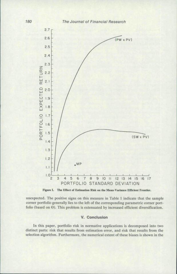
Figure 1 is a graphical presentation of Table 1. For additional comparison, theequivalent of a "market portfolio" (MP), as a single point, is also plotted. This is aportfolio that represents the parametric risk and expected return of equal investmentin each of the 803 stocks in the universe.

In Figure I, both loci represent the average outcome of five hundred samples. Theupper curve represents how the efficient frontier would be constructed, if portfoliomanagers knew the true parametric values of the universe iPW X PV). Note fromTable 1 the consistent, statistically significant overstatement of return (or understate-ment of risk), at any degree of risk aversion. The bottom curve represents the para-metric risk and expected return values of "optimal" portfolios selected from sampledata, and portfolio weights that are produced by these data. These weights are thenapplied to the parametric measures of risk and return. It is clear that internal domi-nance is present (that is, the curve is not strictly convex). Internal dominance indicatesthat corner portfolios formed from sample data are dominated by other corner portfo-lios selected from the same data. This is principally a problem for high-risk portfolios.Thus, portfolio managers would be well advised, as a general rule, to avoid high-risk,high-return portfolios, regardless of the degree of their clients' risk aversion.

It is aiso clear from the data, and from Figure I, that a naive portfolio (MP) evenone with virtually no nonsystematic risk, is inferior to a portfolio that is formed by theMarkowitz-Sharpe algorithm. Note that not only does the higher curve provide domi-nance over MP (a tautology), but so does the lower curve. Thus, the presence of esti-mation risk should not lead to rejection of the selection model.

The vertical difference between the upper curve in Figure I, and the bottomcurve, is the selection bias. This concept helps to explain the complexity of the norma-tive problem. It is interesting to note that this bias is negative, such that its conse-quence is the reduction of total bias. The absolute selection bias is inversely related torisk. The reduction of this bias is the result of diversification. More diversified portfo-lios are, ceteris paribus. more robust to small perturbations of the sample data. Ittakes upward of fifteen stocks to adequately exploit the optimization algorithm (sinceit is being applied to imperfect estimates).

Table 1 reveals that both selection bias and estimation bias decrease with efficientdiversification. The behavior of selection bias in the mean is especially interesting.This bias actually changes signs in the middle of the EF. Thus, well-diversified samplecorner portfolios may have a parametrically higher expected return than the corre-sponding parametric corner portfolio. Naturally, though, these corner portfolios havehigher risk than the corresponding portfolio (i.e., with the same 0) in parameterspace.

As expected, estimation bias in the portfolio mean tends to shrink in absolutevalue as diversification is increased along the EF. It is eliminated near the southwestcomer of the sample EF. The nature of estimation bias in the standard deviation is

180 The Journai of Financiai Research

I-UJor

2.7

2.6

2.5

2.4

2.3

2,1

O 1.9UJQ-X 1 8UJO 1.7O ,6I-or 1.5oQ-

1.4

I.I

1.0

xPV)

(SWx PV)

,MP

3 4 5 6 7 8 9 10 11 12 13 14 15PORTFOLIO STANDARD DEVIATION

16 17

Figure I. Tbe Effect of Estimation Rbk on the Mean-Variance Efficient Frontier.

unexpected. The positive signs on this measure in Table 1 indicate that the samplecorner portfolio generally lies to the left of the corresponding parametric corner port-folio (based on 9). This problem is extenuated by increased efficient diversification.

V. Conclusion

In this paper, portfolio risk in normative applications is decomposed into twodistinct parts: risk that results from estimation error, and risk that results from theselection algorithm. Furthermore, the numerical extent of these biases is shown in the

Estimation and Selection Bias 181

context of a large-scale simulation model; portfolios selected according to the Marko-witz-Sharpe maxim are superior to naive selection rules. Interior dominance in theefficient set exists. This dominance is caused by selection bias, and is a result of under-diversification of high-risk, high-expected-return portfolios. As a general rule, opti-mal portfolios containing at least fifteen stocks are not subject to this interiordominance.

References

1. Alexander. G.. and B. Resnick. "More on Estimation Risk and Simple Rules for Optimal PortfolioSelection." Journal of Finance 40 (March 1985), pp. 125-133.

2. Barry, C. "Effects of Uncertain and Nonstationary Parameters Upon Capital Market EquilibriumConditions." Journal of Financial and Quantitative Analysis 13 (September 1978). pp. 419-433.

3. Best, M. J.. and R. R. Grauer. "Sensitivity Analysis for Mean Variance Portfolio Problems." Work-ing paper, Simon Fraser University. 1986.

4. Brown, S. "The Effect of Estimation Risk on Capital Market Equilibrium." Journal of Financial andQuantitative Analysis 14 (June 1979), pp. 215-220.

5- "Estimation Risk and Optimal Portfolio Choice: The Sharpe Index Model." In Estima-tion Risk and Optimal Portfolio Choice, edited by V. Bawa, C. Brown, and R. Klein, Amster-dam: North-Holland, 1979. pp. 145-171.

6. Elton, E. J.. and M. J. Gruber. "Risk Reduction and Portfolio Size: An Analytical Solution." Journalof Business (October 1977), pp. 415-437.

7. Evans, J. L.. and S. Archer. "Diversification and the Reduction of Dispersion: An Empirical Analy-sis." Journal of Finance 23 (December 1968). pp. 761-769.

8. Frankfurter, G., H. Phillips, and J. Seagle. "Bias in Estimating Portfolio Alpha and Beta Scores."Review of Economics and Statistics 56 (August 1974), pp. 412-414.

9- "Performance of the Sharpe Portfolio Selection Model: A Comparison." Journal of Fi-nancial and Quantitative Analysis 11 (June 1976), pp. 195-204.

10. Frost, P. A., and i. E. Savarino. "An Empirical Bayes Approach to Efficient Portfolio Selection."Journal of Financial und Quantitative Analysis 21 (September 1986), pp. 293-305.

11. Jobson, J. D.. andB. Korkie. "Estimation for Markowitz Efficient Porttohos." Journal of the Ameri-can Statistical Association 75 (September 1980), pp. 544-554.

12. Jorion, P. "Bayes-Stein Estimation for Portfolio Analysis." Journal of Financial and QuantitativeAnalysis 21 (September 1986). pp. 279-292.

13. Kalymon. B. "Estimation Risk in the Portfolio Selection Model." Journal of Financial and Quantita-tive Analysis 6 (March 1971). pp. 559-582.

14. Klein, R., and V. Bawa. "The Effect of Estimation Risk on Optimal Portfolio Choice." Journal ofFinancial Economics 3 (June 1976), pp. 215-231.

' 5 . "The Effect of Limited Information Risk on Optimal Portfolio Diversification." Journalof Financial Economics 5 (August 1977). pp. 89-111.

16. Markowitz, H. "Portfolio Selection." Journal of Finance 7 (March 1952), pp. 77-91.1"̂ - Portfolio Selection: Efficient Diversification of Investments. New York: John Wiley &

Sons, 1959.18. Sharpe, W. "A Simplified Mode! for Portfolio Analysis." Management Science 9 Hanu&ry 1963), pp.

277-293.