
Estimation and Forecasting of Dynamic Conditional ...
30
Estimation and Forecasting of Dynamic Conditional Covariance: A Semiparametric Multivariate Model Xiangdong Long a , Liangjun Su b , Aman Ullah c a Judge Business School, University of Cambridge, [email protected] b School of Economics, Singapore Management University, [email protected] c Department of Economics, University of California, Riverside, [email protected] July 2009 ABSTRACT We propose a semiparametric conditional covariance (SCC) estimator that combines the first-stage parametric conditional covariance (PCC) estimator with the second-stage nonparametric correction estimator in a multiplicative way. We prove the asymptotic normality of our SCC estimator, propose a nonparametric test for the correct specification of PCC models, and study its asymptotic properties. We evaluate the finite sample performance of our test and SCC estimator and compare the latter with that of PCC estimator, purely nonparametric estimator, and Hafner, Dijk, and Franses’s (2006) estimator in terms of mean squared error and Value-at-Risk losses via simulations and real data analyses. JEL Classifications: C3; C5; G0 Key Words: Conditional Covariance Matrix, Multivariate GARCH, Portfolio, Semiparametric Esti- mator, Specification Test. 1
Transcript of Estimation and Forecasting of Dynamic Conditional ...

Estimation and Forecasting of Dynamic Conditional
Covariance: A Semiparametric Multivariate Model
Xiangdong Longa, Liangjun Sub, Aman Ullahc
aJudge Business School, University of Cambridge, [email protected] of Economics, Singapore Management University, [email protected]
cDepartment of Economics, University of California, Riverside, [email protected]
July 2009
ABSTRACT
We propose a semiparametric conditional covariance (SCC) estimator that combines the first-stage
parametric conditional covariance (PCC) estimator with the second-stage nonparametric correction
estimator in a multiplicative way. We prove the asymptotic normality of our SCC estimator, propose a
nonparametric test for the correct specification of PCC models, and study its asymptotic properties. We
evaluate the finite sample performance of our test and SCC estimator and compare the latter with that
of PCC estimator, purely nonparametric estimator, and Hafner, Dijk, and Franses’s (2006) estimator in
terms of mean squared error and Value-at-Risk losses via simulations and real data analyses.
JEL Classifications: C3; C5; G0
Key Words: Conditional Covariance Matrix, Multivariate GARCH, Portfolio, Semiparametric Esti-
mator, Specification Test.
1

1 INTRODUCTION
Since the seminal work of Engle (1982), there has developed a huge literature on modeling the time-
varying volatility of economic data in univariate case. Nevertheless, for asset allocation, risk manage-
ment, hedging and asset pricing, multivariate generalized autoregressive conditional heteroskedasticity
(MGARCH) models are of more importance both theoretically and practically because they model the
volatility and co-volatility of multiple financial assets jointly. Many recent works have been done in
the area of MGARCH models, such as the VECH model of Bollerslev, Engle and Wooldridge (1988),
the BEKK model of Baba, Engle, Kraft, and Kroner (1991) and Engle and Kroner (1995), the dy-
namic conditional correlation (DCC) model of Engle (2002) and Engle and Sheppard (2001), the Factor
GARCH model of Engle, Ng and Rothschild (1990), to name just a few. However, all these existing
MGARCH models share two common features: the normality assumption on the error’s distribution
and the linearity of dynamic conditional covariance matrix. The exceptions include the regime switching
dynamic conditional correlation model of Pelletier (2006), the smooth transition conditional correlation
(STCC) model by Silvennoinen and Teräsvirta (2005), and the asymmetric dynamic conditional correla-
tion model by Cappiello, Engle and Sheppard (2003), where parametric nonlinear conditional correlation
models are used with Gaussian errors, and the copula-based MGARCH model by Lee and Long (2009),
where copula is used to construct non-Gaussian errors. The normality assumption is rejected by Fama
and French (1993), Richardson and Smith (1993), Longin and Solnik (2001), Ang and Chen (2002), and
Mashal and Zeevi (2002), etc. The linear dynamic assumption excludes possible nonlinearity. Once we
diverge from linearity, there is too much freedom to specify nonlinearity.
In this paper, we propose a semiparametric conditional covariance (SCC) model, which combines
parametric and nonparametric estimators of conditional covariance matrix in a multiplicative way. We
first model the conditional covariance matrix parametrically just like what we do for the conventional
parametric MGARCH models. Then we model the conditional covariance of the standardized residuals
nonparametrically. The estimate of the latter will serve as a nonparametric correction factor for the
parametric conditional covariance (PCC) estimator. Such combined estimation has been done by Olkin
and Speigelman (1987) in density function, by Glad (1998) in conditional mean estimation, and by
Mishra, Su, and Ullah (2009) in conditional variance estimation. Nevertheless, to our knowledge, there
is no such a combined estimator for conditional covariance matrix.
We provide asymptotic theory for our semiparametric estimator. It possesses several advantages
over both pure parametric and nonparametric estimators. First, our SCC model avoids the common
shortcomings of parametric MGARCH models on potential misspecifications of functional form and
density function. It does not rely on either the distributional assumption on the error term or the
parametric functional form of the conditional covariance matrix. Second, when the parametric model is
misspecified, the parametric estimator of the conditional covariance is generally inconsistent despite the
fact that the finite dimensional parameter in the parametric model may converge to some pseudo-true
parameter (see White, 1994). In contrast, our semiparametric estimator can still be consistent with
the true conditional covariance matrix under certain conditions. Third, when the parametric model
is correctly specified, as expected, our semiparametric estimator is less efficient than the parametric
2

estimator but it can achieve the parametric convergence rate with a fixed bandwidth.
The original contribution to the literature lies in three aspects. First, we are among the first to
consider combined estimators of conditional covariance matrix. Our SCC estimators can be regarded
as an extension of Mishra, Su, and Ullah (2009) from the conditional variance (one-dimension) case to
the conditional covariance (multi-dimension) case. For notational simplicity, we focus on local constant
(Nadaraya-Watson) estimation instead of local polynomial estimation. Our new findings suggest that the
proposed SCC estimator has the same asymptotic variance as the one-step nonparametric conditional
covariance (NCC) estimator but different asymptotic biases. Second, based on the estimator of the
nonparametric correction factor, we propose a formal test for the correct specification of PCC models,
which has not been addressed in earlier literature on combined estimation. Third, our theoretical results
are validated via Monte Carlo simulations and real data analyses.
We report a small set of Monte Carlo simulation results to evaluate the finite sample performance
of our nonparametric test and SCC estimator and compare the latter with that of the PCC estimator,
the NCC estimator and Hafner, Dijk, and Franses’s (2006, HDF hereafter) semiparametric estimator.
The data generating processes (DGPs) used in our simulations are motivated by the nonlinear and
non-normal stylized facts widely observed in financial data, for instance, conditional correlation tends
to be high during the crisis period and low during the tranquil period. Simulations suggest that our
nonparametric test for the correct specification of PCCmodels performs reasonably well in finite samples.
For comparison across different estimators, we use both mean squared error (MSE) and 1% Value-at-
Risk (VaR) losses. To evaluate portfolio’s VaR loss, we consider two portfolio weighting mechanisms,
namely equal weight (EW) and minimum variance weight (MVW). We find that our semiparametric
estimators tend to outperform their parametric counterparts and the NCC and HDF’s estimators.
In empirical analysis, we carry out in-sample (IS) estimation and out-of-sample (OoS) forecasting
for the conditional covariance matrix of paired market indices in three datasets. Our nonparametric
tests reject all commonly used PCC models for all three datasets at the 1% significance level. This
is in favor of the use of a semiparametric or nonparametric estimator for the conditional covariance.
When we fit the datasets by our SCC model, the PCC model, the NCC model, and the HDF model,
we find that our SCC model can always reduce the IS losses of the start-up PCC model regardless of
portfolio weights, generally reduces the OoS losses over the PCC models, and tends to perform best
across different models.
The rest of the paper is organized as follow. We briefly review some PCC models in Section 2.
In Section 3 we present our SCC model and estimator, propose a nonparametric test for the correct
specification of PCC models, and study their asymptotic properties under the null hypothesis and a
sequence of local alternatives. In Section 4 we provide a small set of Monte Carlo experiments to evaluate
the finite sample performance of our SCC estimators and nonparametric test, and apply all conditional
covariance models on three paired stock indices. All proofs are relegated to Appendix.
To proceed, we define some notation that will be used throughout the paper. Let Ik denote a k × k
identity matrix. Let z =(z1, ..., zk)0 be a k × 1 vector and Z be a symmetric k × k matrix with (i, j)th
element zij . The Euclidean norm of z or Z is denoted as kzk or kZk .We define the following operators:diag(Z) denotes the diagonal matrix with zi in the (i, i)th place; Z∗ denotes a diagonal matrix with the
3

square roots of the diagonal elements of Z on its diagonal when Z is positive definite; vec(Z) stacks the
columns of Z into a k2× 1 vector; vech(Z) stacks the lower triangular part of Z (including the diagonalelements) into a k (k + 1) /2 × 1 vector. Further, we use Dk to denote the k2 × (k (k + 1) /2) uniqueduplication matrix and D+
k to denote its generalized inverse, which is of size (k (k + 1) /2) × k2. That
is, vec(Z) = Dkvech(Z) , vech(Z) = D+k vec(Z) , D
+k = (D
0kDk)
−1D0k and D+
k Dk = Ik(k+1)/2. Here we
have used the fact that D0kDk is nonsingular. Let Nk ≡ DkD
+k . We will use the following properties of
Nk: Nk is symmetric, NkDk = Dk, NkD+0k = D+0
k , and Nk(A⊗A) = (A⊗A)Nk, where A is a k × k
matrix. For more details, see Magnus and Neudecker (1999, pp. 48-50).
2 PARAMETRIC CONDITIONAL COVARIANCEMODELS
Suppose the return series rtTt=1 of the interested financial data follows the stochastic process:
rt|Ft−1 ∼ P(μt,Ht; θ), t = 1, ..., T, (2.1)
where rt ≡ (r1t, . . . , rkt)0 is an k × 1 vector, Ft−1 is the information set (σ-field) at time t − 1,
E(rt|Ft−1) = μt, E(rtr0t|Ft−1) = Ht, Ht is the conditional covariance matrix, and P is the joint
cumulative distribution function (CDF) of rt, and θ represents the parameters in the distribution. Like
Engle (2002), for simplicity we assume the conditional mean μt is zero. If not, necessary standardization
should be applied on the data. Thus we can write the model for rt as
rt =H1/2t et, (2.2)
where et ≡ H−1/2t rt is the standardized error with E(et|Ft−1) = 0 and E(ete
0t|Ft−1) = Ik. et is
typically assumed to follow the standard normal distribution: et ∼ iid N(0, Ik). We are interested in
estimating the conditional covariance matrix Ht of rt without such a distributional assumption.
The conditional covariance matrix Ht can be decomposed as
Ht = Dt (θ)Rt (θ)Dt (θ) , (2.3)
where Rt (θ) is the conditional correlation matrix with the (i, j)th element denoted as ρij,t (θ) , which
stands for the conditional correlation between rit and rjt and can be time-varying; Dt (θ) =diag(ph1,t,
...,phk,t) is a diagonal matrix with the square root of the conditional variances hi,t, parameterized
by the vector θ, on the diagonal. It is well known (e.g., Engle, 2002) that the conditional correlation
matrix Rt (θ) is also the conditional covariance matrix of the standardized returns εt ≡ (ε1t, . . . , εkt)0 =D−1t (θ) rt, i.e., E(εtε0t|Ft−1) = Rt (θ) .
Now we review some popular parametric models for the conditional covariance matrix Ht, which
will be used in Section 4. These models stem from two different modeling methodologies. First, the
BEKK model specifies the elements of Ht directly:
Ht= δδ0+Σpi=1AiHt−iA0i +Σ
qj=1Bj
¡rt−jr
0t−j¢B0j , (2.4)
where δ is a k×k low-triangle matrix, and different matrix properties ofAi and Bj lead to three types of
BEKK models: the matrices Ai and Bj in the full, diagonal, and scalar BEKK models are full matrices,
4

diagonal matrices, and scalars, respectively. Second, instead of modeling the conditional covariance
matrix directly, observing Ht= DtRtDt in (2.3), one can model Ht indirectly through modeling Dt and
Rt separately. The resulting models include the CCC model by Bollerslev (1990), the VC model by
Tse and Tsui (2002), the DCC model by Engle (2002), among others. The CCC model assumes that
Rt = R, a constant matrix, and hence the time-varying feature of conditional covariance could only be
attributed to the time-varying conditional variances. The VC model by Tse and Tsui (2002) specifies
univariate GARCH(p, q) models for individual returns and GARCH-type dynamic evolutions for the
conditional correlation process Rt:
Rt =¡1− Σpi=1γi − Σ
qj=1βj
¢R+Σpi=1γiRt−i +Σ
qj=1βj
bRt−j , (2.5)
where R, Rt, and bRt are the unconditional, conditional, and sample correlation matrices at time t
with unit diagonal elements. Similar to the CCC and VC models, the DCC model also uses two-stage
modeling strategy. In the first stage, one models the conditional variance processes with the usual
univariate GARCH models and then obtains the standardized residual εt. In the second stage, one
models the conditional covariance Qt of εt as
Qt =¡1− Σpi=1γi − Σ
qj=1βj
¢Q+Σpi=1γiQt−i +Σ
qj=1βj(bεt−jbε0t−j), (2.6)
where Q is the sample covariance matrix for εt. The basic properties of correlation matrix, such as
positive definiteness and unit diagonal element, are ensured by using the transformation
Rt = Q∗−1t QtQ
∗−1t (2.7)
where Q∗t is a diagonal matrix with the square roots of the diagonal elements of Qt on its diagonal.
In all the above models, the functional form of conditional covariance matrix is assumed to be
of known and the maximum likelihood estimation is done under the assumption of normality. These
assumptions will not be required for the semiparametric estimators introduced below.
3 ANALTERNATIVE SEMIPARAMETRICCONDITIONAL
COVARIANCE ESTIMATOR
In this section we first review HDF’s semiparametric estimator and propose an alternative semipara-
metric estimator for the conditional covariance matrix. We then study the asymptotic properties of our
SCC estimator and propose a nonparametric test for the correct specification of PCC models.
3.1 HDF’s Semiparametric Estimator
Motivated by the idea that the conditional correlations depend on exogenous factors such as the market
return or volatility, HDF propose the following semiparametric model for rt :
rt = Dt (θ) εt, E (εt|Ft−1) = 0, E (εtε0t|Ft−1) = R (xt) , (3.1)
5

where Dt (θ) is as defined before (after (2.3)), and xt is observable at time t − 1 and xt ∈ Ft−1.Assuming that θ can be estimated by bθ at the parametric √T -rate, they define standardized residualsby eεt ≡ εt(bθ) = Dt(bθ)−1rt. Then they regress eεteε0t on xt nonparametrically to obtain eQ (x) , theNadaraya-Watson kernel estimator of E
¡eεteε0t|xt = x¢ . Their semiparametric conditional correlationmatrix estimator is defined by
eR (x) = (eQ∗ (x))−1 eQ (x) (eQ∗ (x))−1, (3.2)
where eQ∗ (x) is a diagonal matrix with the square roots of the diagonal elements of eQ (x) on itsdiagonal. Their semiparametric estimator of Ht can be written as follows
eHt = Dt(bθ)eR (xt)Dt(bθ). (3.3)
Clearly, the HDF’s estimators require correct specification of the conditional variance process in
order to obtain a final consistent conditional correlation or covariance estimator. This is unsatisfactory
since it is extremely hard to know a prior the correct form of the conditional variance process. Below
we propose an alternative SCC estimator that can be consistent even if the conditional variance process
may be misspecified in the first stage and it requires similar assumption to that in (3.1).
3.2 An Alternative Semiparametric Estimator
Motivated by Glad (1998) and Mishra, Su, and Ullah (2009), we propose an alternative SCC estimator,
which combines in a multiplicative way the parametric conditional covariance estimator from the first
stage with the nonparametric conditional covariance estimator from the second stage. Essentially, this
estimator nonparametrically adjusts the initial PCC estimator.
Let Ht = E (rtr0t|Ft−1) be the true time-varying conditional covariance process:
rt =H1/2t et, E (et|Ft−1) = 0, E (ete0t|Ft−1) = Ik, (3.4)
where H1/2t is the symmetric square root matrix of Ht. Let Hp,t (θ) be a parametrically-specified
time-varying conditional covariance process for rt, where θ ∈ Θ ⊂ Rp and Hp,t (θ) ∈ Ft−1. Analogousto Mishra, Su, and Ullah (2009), our estimation strategy builds on the simple identity
Ht =Hp,t (θ)1/2E
£et (θ) et (θ)
0 |Ft−1¤Hp,t (θ)
1/2 , (3.5)
where Hp,t (θ)1/2 is the symmetric square root matrix of Hp,t (θ) , and et (θ) = Hp,t (θ)
−1/2rt is the
standardized error from the parametric model. When θ = θ∗, some pseudo-true parameter value, we
write Hp,t = Hp,t (θ∗) and et = et (θ∗) . It is clear that the parametric component Hp,t (θ) in (3.5)
can be any PCC model reviewed in Section 2 and estimated by some standard parametric method. To
propose a reasonable estimator for the nonparametric component E£et (θ) et (θ)
0 |Ft−1¤, we follow the
HDF’s idea and assume that the conditional expectation of ete0t depends on the current information set
Ft−1 only through a q × 1 observable vector xt = (x1t, ..., xqt)0 . That is,
E [ete0t|Ft−1] = Gnp (xt) , (3.6)
6
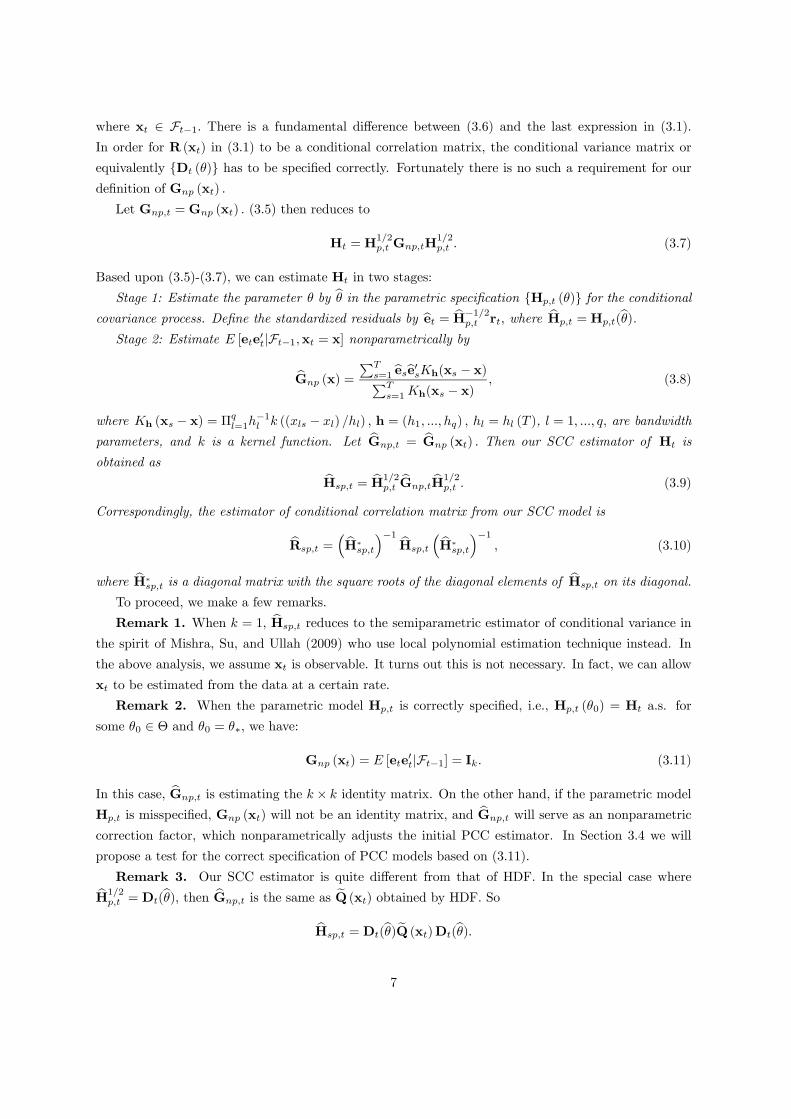
where xt ∈ Ft−1. There is a fundamental difference between (3.6) and the last expression in (3.1).In order for R (xt) in (3.1) to be a conditional correlation matrix, the conditional variance matrix or
equivalently Dt (θ) has to be specified correctly. Fortunately there is no such a requirement for ourdefinition of Gnp (xt) .
Let Gnp,t =Gnp (xt) . (3.5) then reduces to
Ht =H1/2p,t Gnp,tH
1/2p,t . (3.7)
Based upon (3.5)-(3.7), we can estimate Ht in two stages:
Stage 1: Estimate the parameter θ by bθ in the parametric specification Hp,t (θ) for the conditionalcovariance process. Define the standardized residuals by bet = bH−1/2p,t rt, where bHp,t =Hp,t(bθ).Stage 2: Estimate E [ete
0t|Ft−1,xt = x] nonparametrically by
bGnp (x) =
PTs=1 besbe0sKh(xs − x)PT
s=1Kh(xs − x), (3.8)
where Kh (xs − x) = Πql=1h−1l k ((xls − xl) /hl) , h = (h1, ..., hq) , hl = hl (T ), l = 1, ..., q, are bandwidth
parameters, and k is a kernel function. Let bGnp,t = bGnp (xt) . Then our SCC estimator of Ht is
obtained as bHsp,t = bH1/2p,tbGnp,t
bH1/2p,t . (3.9)
Correspondingly, the estimator of conditional correlation matrix from our SCC model is
bRsp,t =³bH∗sp,t´−1 bHsp,t
³bH∗sp,t´−1 , (3.10)
where bH∗sp,t is a diagonal matrix with the square roots of the diagonal elements of bHsp,t on its diagonal.
To proceed, we make a few remarks.
Remark 1. When k = 1, bHsp,t reduces to the semiparametric estimator of conditional variance in
the spirit of Mishra, Su, and Ullah (2009) who use local polynomial estimation technique instead. In
the above analysis, we assume xt is observable. It turns out this is not necessary. In fact, we can allow
xt to be estimated from the data at a certain rate.
Remark 2. When the parametric model Hp,t is correctly specified, i.e., Hp,t (θ0) = Ht a.s. for
some θ0 ∈ Θ and θ0 = θ∗, we have:
Gnp (xt) = E [ete0t|Ft−1] = Ik. (3.11)
In this case, bGnp,t is estimating the k × k identity matrix. On the other hand, if the parametric model
Hp,t is misspecified, Gnp (xt) will not be an identity matrix, and bGnp,t will serve as an nonparametric
correction factor, which nonparametrically adjusts the initial PCC estimator. In Section 3.4 we will
propose a test for the correct specification of PCC models based on (3.11).
Remark 3. Our SCC estimator is quite different from that of HDF. In the special case wherebH1/2p,t = Dt(bθ), then bGnp,t is the same as eQ (xt) obtained by HDF. So
bHsp,t = Dt(bθ)eQ (xt)Dt(bθ).7
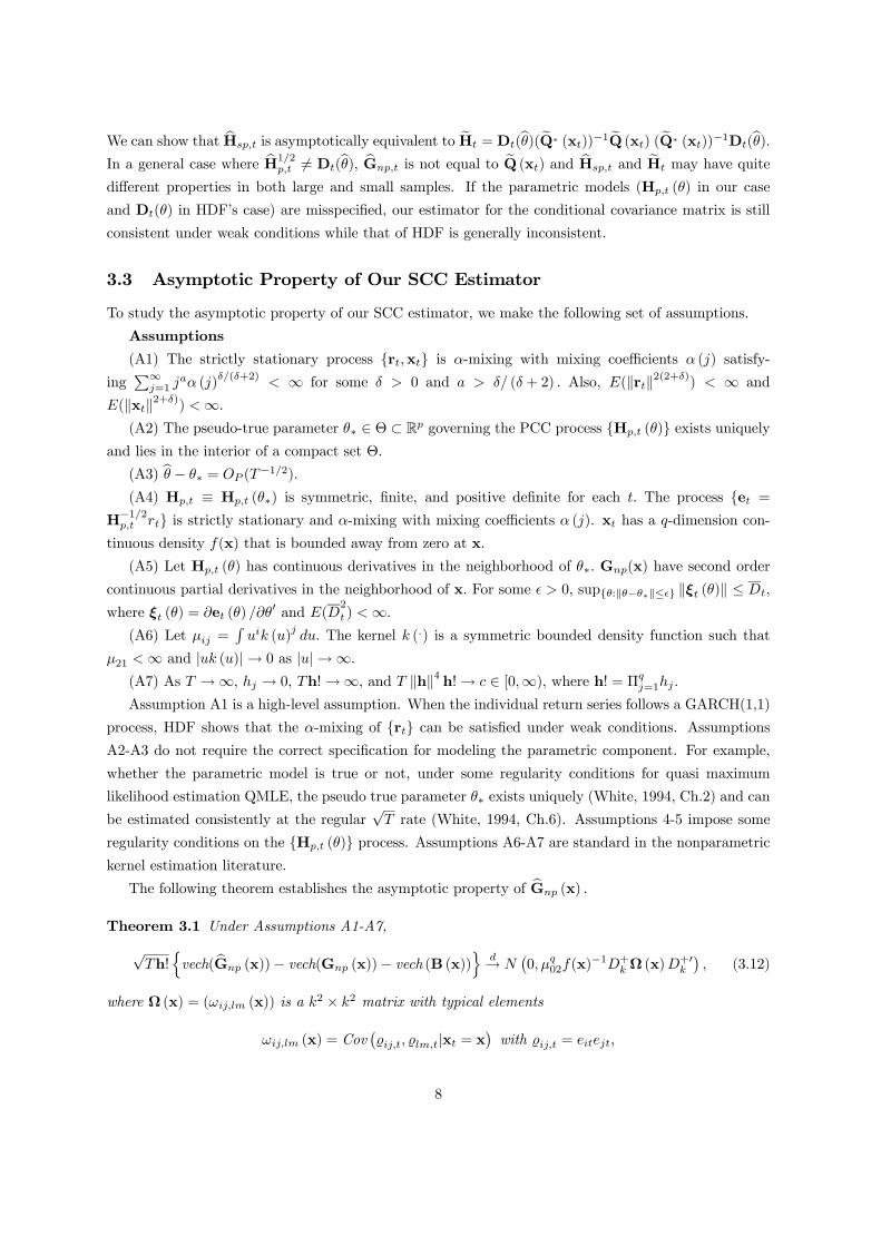
We can show that bHsp,t is asymptotically equivalent to eHt = Dt(bθ)(eQ∗ (xt))−1 eQ (xt) (eQ∗ (xt))−1Dt(bθ).In a general case where bH1/2
p,t 6= Dt(bθ), bGnp,t is not equal to eQ (xt) and bHsp,t and eHt may have quite
different properties in both large and small samples. If the parametric models (Hp,t (θ) in our case
and Dt(θ) in HDF’s case) are misspecified, our estimator for the conditional covariance matrix is still
consistent under weak conditions while that of HDF is generally inconsistent.
3.3 Asymptotic Property of Our SCC Estimator
To study the asymptotic property of our SCC estimator, we make the following set of assumptions.
Assumptions
(A1) The strictly stationary process rt,xt is α-mixing with mixing coefficients α (j) satisfy-
ingP∞
j=1 jaα (j)δ/(δ+2) < ∞ for some δ > 0 and a > δ/ (δ + 2) . Also, E(krtk2(2+δ)) < ∞ and
E(kxtk2+δ)) <∞.(A2) The pseudo-true parameter θ∗ ∈ Θ ⊂ Rp governing the PCC process Hp,t (θ) exists uniquely
and lies in the interior of a compact set Θ.
(A3) bθ − θ∗ = OP (T−1/2).
(A4) Hp,t ≡ Hp,t (θ∗) is symmetric, finite, and positive definite for each t. The process et =H−1/2p,t rt is strictly stationary and α-mixing with mixing coefficients α (j). xt has a q-dimension con-
tinuous density f(x) that is bounded away from zero at x.
(A5) Let Hp,t (θ) has continuous derivatives in the neighborhood of θ∗. Gnp(x) have second order
continuous partial derivatives in the neighborhood of x. For some > 0, supθ:kθ−θ∗k≤ kξt (θ)k ≤ Dt,
where ξt (θ) = ∂et (θ) /∂θ0 and E(D
2
t ) <∞.
(A6) Let μij =Ruik (u)
jdu. The kernel k (.) is a symmetric bounded density function such that
μ21 <∞ and |uk (u)|→ 0 as |u|→∞.
(A7) As T →∞, hj → 0, Th!→∞, and T khk4 h!→ c ∈ [0,∞), where h! = Πqj=1hj .Assumption A1 is a high-level assumption. When the individual return series follows a GARCH(1,1)
process, HDF shows that the α-mixing of rt can be satisfied under weak conditions. AssumptionsA2-A3 do not require the correct specification for modeling the parametric component. For example,
whether the parametric model is true or not, under some regularity conditions for quasi maximum
likelihood estimation QMLE, the pseudo true parameter θ∗ exists uniquely (White, 1994, Ch.2) and can
be estimated consistently at the regular√T rate (White, 1994, Ch.6). Assumptions 4-5 impose some
regularity conditions on the Hp,t (θ) process. Assumptions A6-A7 are standard in the nonparametrickernel estimation literature.
The following theorem establishes the asymptotic property of bGnp (x) .
Theorem 3.1 Under Assumptions A1-A7,
√Th!
nvech( bGnp (x))− vech(Gnp (x))− vech (B (x))
od→ N
¡0, μq02f(x)
−1D+k Ω (x)D
+0k
¢, (3.12)
where Ω (x) = (ωij,lm (x)) is a k2 × k2 matrix with typical elements
ωij,lm (x) = Cov¡
ij,t, lm,t|xt = x¢with ij,t = eitejt,
8

B (x) = (Bij (x)) is a k × k matrix with typical elements
Bij (x) =μ212f (x)
qXl=1
∙2∂f (x)
∂xl
∂Gnp,ij (x)
∂xl+ f (x)
∂2Gnp,ij (x)
∂xl∂xl
¸h2l ,
where eit is the ith element of et and Gnp,ij (x) is the (i, j)th element of Gnp (x) .
Remark 4. Theorem 3.1 implies that we can estimate Gnp (x) consistently by bGnp (x) , which has
the usual asymptotic bias and variance structure as typical local constant estimators. Let ηt =vech(ete0t).
We can get an alternative expression for D+k Ω (x)D
+0k :
D+k Ω (x)D
+0k = Var (ηt|xt = x) .
When the start-up PCC model is correctly specified, i.e., Ht = Hp,t (θ∗) , then Gnp (x) = Ik, and the
asymptotic bias term in (3.12) vanishes (B (x) = 0).
The asymptotic property of our semiparametric estimator for the conditional covariance matrix Ht
is stated in the following corollary.
Corollary 3.2 (i) For any xt such that f (xt) is bounded away from 0, bHsp,t and bRsp,t are consistent
for Ht and Rt, respectively. That is,
bHsp,t = bH1/2p,tbGnp,t
bH1/2p,t
p→Ht, and bRsp,t =³bH∗sp,t´−1 bHsp,t
³bH∗sp,t´−1 p→ Rt.
(ii)√Th!
nvech
³bHsp,t
´− vech (Ht)−Bt (xt)
od→MN
¡0, μq02f(xt)
−1D+k Ωt (xt)D
+0k
¢, where Bt (x)
=vech³H1/2p,t B (x)H
1/2p,t
´and Ωt (x) =
³H1/2p,t ⊗H
1/2p,t
´Ω (x)
³H1/2p,t ⊗H
1/2p,t
´. That is, conditional on
Hp,t and xt,√Th!
nvech
³bHsp,t
´− vech (Ht)−Bt (xt)
ois asymptotically normal with mean zero and
variance μq02f(xt)−1D+
k Ωt (xt)D+0k .
Remark 5. Corollary 3.2(i) says that we can obtain a consistent estimator for the conditional
covariance and correlation matrix. Corollary 3.2(ii) essentially says that bHsp,t is also asymptotically
normally distributed conditional on Hp,t and xt, and it inherits the asymptotic bias and variance
structure of bGnp (xt) . By the delta method, one can also show that the semiparametric estimator for
conditional correlation matrix is also asymptotically distributed with the nonparametric convergence
rate√Th!.
Remark 6. To compare our estimator with the parametric estimator of conditional covariance,
first note that when the parametric component is correctly specified, as expected, our estimator is less
efficient than the parametric one since our estimator has a slower convergence rate than the parametric
estimator as khk→ 0. Nevertheless, when h is kept fixed, a careful examination of the proof of Theorem
3.1 and Corollary 3.2 indicates that our semiparametric estimator is consistent with the true conditional
covariance with the regular parametric√T -rate of convergence. In this sense, we say that our estimator
is almost as good as the parametric estimator in terms of convergence rate when h is kept fixed. Next,
in the case of misspecification, the PCC estimator is usually inconsistent (even though bθ is consistentfor some pseudo-true parameter θ∗) while our semiparametric conditional covariance estimator is still
consistent. Similar remarks hold true for the estimators of conditional correlation matrix.
9
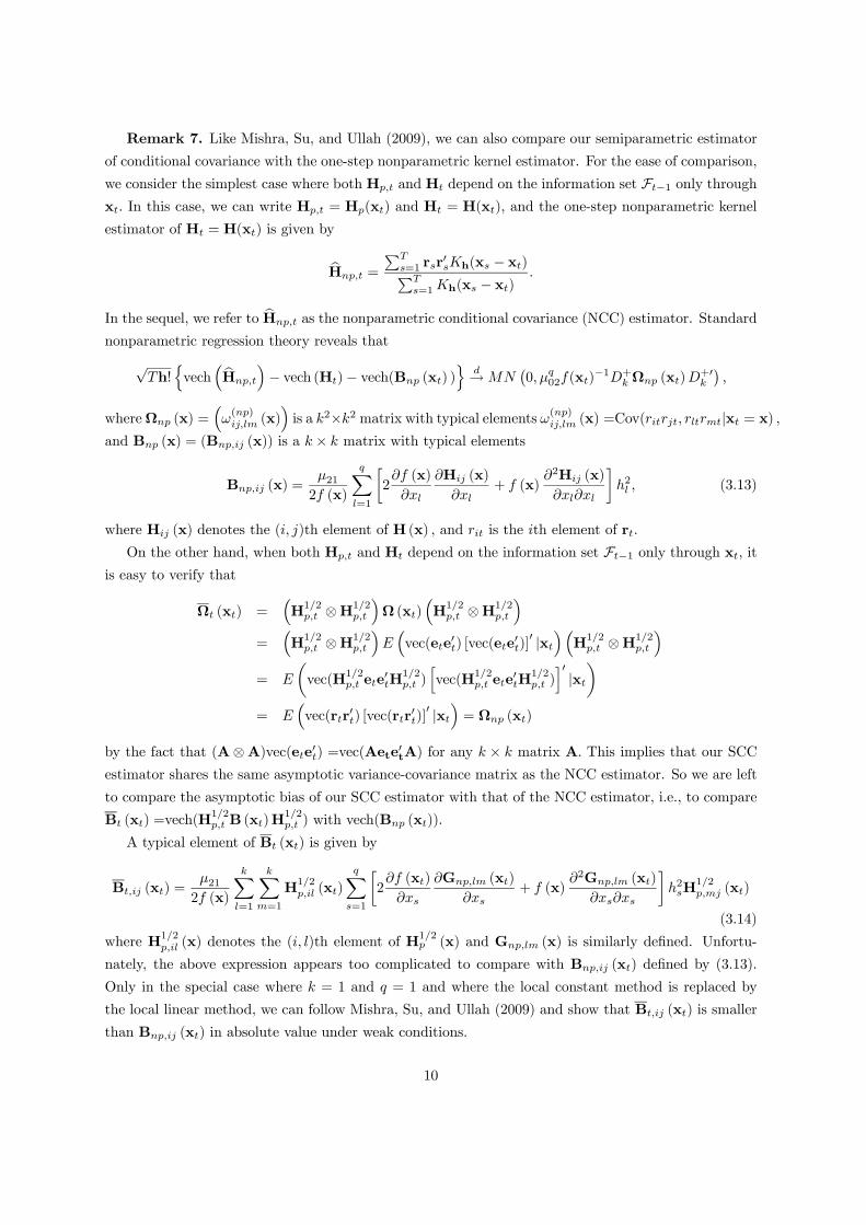
Remark 7. Like Mishra, Su, and Ullah (2009), we can also compare our semiparametric estimator
of conditional covariance with the one-step nonparametric kernel estimator. For the ease of comparison,
we consider the simplest case where both Hp,t and Ht depend on the information set Ft−1 only throughxt. In this case, we can write Hp,t = Hp(xt) and Ht = H(xt), and the one-step nonparametric kernel
estimator of Ht = H(xt) is given by
bHnp,t =
PTs=1 rsr
0sKh(xs − xt)PT
s=1Kh(xs − xt).
In the sequel, we refer to bHnp,t as the nonparametric conditional covariance (NCC) estimator. Standard
nonparametric regression theory reveals that
√Th!
nvech
³bHnp,t
´− vech (Ht)− vech(Bnp (xt) )
od→MN
¡0, μq02f(xt)
−1D+k Ωnp (xt)D
+0k
¢,
whereΩnp (x) =³ω(np)ij,lm (x)
´is a k2×k2 matrix with typical elements ω(np)ij,lm (x) =Cov(ritrjt, rltrmt|xt = x) ,
and Bnp (x) = (Bnp,ij (x)) is a k × k matrix with typical elements
Bnp,ij (x) =μ212f (x)
qXl=1
∙2∂f (x)
∂xl
∂Hij (x)
∂xl+ f (x)
∂2Hij (x)
∂xl∂xl
¸h2l , (3.13)
where Hij (x) denotes the (i, j)th element of H (x) , and rit is the ith element of rt.
On the other hand, when both Hp,t and Ht depend on the information set Ft−1 only through xt, itis easy to verify that
Ωt (xt) =³H1/2p,t ⊗H
1/2p,t
´Ω (xt)
³H1/2p,t ⊗H
1/2p,t
´=
³H1/2p,t ⊗H
1/2p,t
´E³vec(ete0t) [vec(ete
0t)]0 |xt
´³H1/2p,t ⊗H
1/2p,t
´= E
µvec(H1/2
p,t ete0tH
1/2p,t )
hvec(H1/2
p,t ete0tH
1/2p,t )
i0|xt
= E³vec(rtr0t) [vec(rtr
0t)]0 |xt
´= Ωnp (xt)
by the fact that (A⊗A)vec(ete0t) =vec(Aete0tA) for any k × k matrix A. This implies that our SCC
estimator shares the same asymptotic variance-covariance matrix as the NCC estimator. So we are left
to compare the asymptotic bias of our SCC estimator with that of the NCC estimator, i.e., to compare
Bt (xt) =vech(H1/2p,t B (xt)H
1/2p,t ) with vech(Bnp (xt)).
A typical element of Bt (xt) is given by
Bt,ij (xt) =μ212f (x)
kXl=1
kXm=1
H1/2p,il (xt)
qXs=1
∙2∂f (xt)
∂xs
∂Gnp,lm (xt)
∂xs+ f (x)
∂2Gnp,lm (xt)
∂xs∂xs
¸h2sH
1/2p,mj (xt)
(3.14)
where H1/2p,il (x) denotes the (i, l)th element of H
1/2p (x) and Gnp,lm (x) is similarly defined. Unfortu-
nately, the above expression appears too complicated to compare with Bnp,ij (xt) defined by (3.13).
Only in the special case where k = 1 and q = 1 and where the local constant method is replaced by
the local linear method, we can follow Mishra, Su, and Ullah (2009) and show that Bt,ij (xt) is smaller
than Bnp,ij (xt) in absolute value under weak conditions.
10

3.4 Test for the Correct Specification of PCC Models
In this subsection we propose a test of correct specification of parametric conditional covariance models
based on (3.11). The null hypothesis is
H0 : Gnp (xt) = Ik a.s. (3.15)
and the alternative hypothesis is
H1 : Pr (Gnp (xt) = Ik) < 1. (3.16)
Let σij (x) denote the (i, j) element of Gnp (x) , i, j = 1, · · · , k. That is, σij (xt) = E [eitejt|Ft−1] ,where recall eit denotes the ith element of et. We can rewrite the null hypothesis as
H0 : P (σij (xt) = δij) = 1 for all i, j = 1, · · · , k, (3.17)
and the alternative hypothesis as
H1 : Pr (σij (xt) = δij) < 1 for some i, j = 1, · · · , k, (3.18)
where δij is Kronecker’s delta, i.e., δij = 1 if i = j and 0 otherwise.
Recall that f (x) denotes the density function of xt. When the null and alternative hypotheses are
written in the form of (3.17) and (3.18), we can construct consistent tests of H0 versus H1 using various
distance measures. A convenient choice is to use the measure
Γ =k−1Xi=1
kXj=i
Z(σij (x)− δij)
2 f2 (x) dx ≥ 0 (3.19)
and Γ = 0 if and only if H0 given by (3.17) holds. Note that the use of density weight in the definition
of Γ will help us avoid the random denominator issue. We will propose a test statistic based upon a
kernel estimator of Γ.
To construct the sample analog of Γ, we first obtain estimators of σij (x) and f (x) , which are given
by
bσij (x) = T−1PT
s=1 beitbejtKh(xs − x)bf (x) , and bf (x) = T−1TXs=1
Kh(xs − x), (3.20)
where beit is the ith element of bet. Note that bσij (x) is the (i, j) element of bGnp (xt) . We then estimate
Γ by the following functional:
bΓ1 =k−1Xi=1
kXj=i
Z(bσij (x)− δij)
2 bf2 (x) dx=
1
T 2
k−1Xi=1
kXj=i
TXs=1
TXt=1
(beisbejs − δij) (beitbejt − δij)Kh (xs − xt) (3.21)
where Kh (u) = Πql=1h
−1l k (ul/hl) , u = (u1, · · · , uq), and k (u) =
Rk (v) k (u− v) dv is the convolution
kernel derived from k. For example, if k (u) = exp¡−u2/2
¢/√2π, then k (u) = exp
¡−u2/4
¢/√4π, a
normal density with zero mean and variance 2.
11

The above statistic is simple to compute and offers a natural way to test H0 in (3.17). Nevertheless,
we propose a bias-adjusted test statistic, namely,
bΓ = 1
T 2
k−1Xi=1
kXj=i
TXs=1
TXt6=s
(beisbejs − δij) (beitbejt − δij)Kh (xs − xt) . (3.22)
In effect, bΓ removes the “diagonal” (s = t) terms from bΓ1 in (3.21), thus reducing the bias of the statistic.A similar idea has been used in Lavergne and Vuong (2000), Su and White (2007), and Su and Ullah
(2009). We will show that after being appropriately scaled, bΓ is asymptotically normally distributedunder suitable assumptions.
To derive the asymptotic properties of the test statistic bΓ, we add the following assumptions.Assumptions
(A8) Let εijt ≡ eitejt−δij . For i, j = 1, · · · , k, E¡|εijt|4(1+δ)
¢≤ C and E
¯εr1ijt1ε
r2ijt2
· · · εrlijtl¯1+δ ≤ C
for some C <∞, where 2 ≤ l ≤ 4, 0 ≤ rs ≤ 4, andPl
s=1 rs ≤ 8.(A9) (i) Let μij2 (x) ≡ E(ε2ijt|xt = x) and μij4 (x) = E(ε4ijt|xt = x). Both μij2 (x) and μij4 (x)
satisfy the Lipschitz condition: for i, j = 1, · · · , k and l = 2, 4, |μijl (x+ x∗)− μijl (x) | ≤ dijl (x) kx∗k ,where k.k denotes the Euclidean norm and
Rdijl (x) f (x) dx < C <∞. (ii) The joint density ft1,...,tl (.)
of (xi1 , ...,xil) (1 ≤ l ≤ 4) exists and satisfies the Lipschitz condition: |ft1,...,tl¡x(1) + v(1), ...,x(l) + v(l)
¢−ft1,...,tl
¡x(1), ...,x(l)
¢| ≤ Dt1,...,tl
¡x(1), ...,x(l)
¢kvk, where v0 = (v(1)0 , ...,v(l)0),
RDt1,...,tl
¡v(1), ...,v(l)
¢kvk2(1+δ) dv ≤ C and
RDt1,...,tl(v
(1), ...,v(l)) ft1,...,tl(v(1), ..., v(l))dv ≤ C for some C <∞.
Assumptions A8-A9 are common in nonparametric estimation with strong mixing data (see Gao and
King, 2003). They are mainly used in the proof of Theorem 3.3 below.
Define
σ20 ≡ 2Z
K2(u) du
k−1Xi1=1
kXj1=i1
k−1Xi2=1
kXj2=i2
E[b2i1j1i2j2(xt)f (xt)],
where bi1j1i2j2(x) = E [(ei1tej1t − δi1j1) (ei2tej2t − δi2j2) |xt = x] , and K (u) = Πql=1k (ul) . The asymp-
totic null distribution of bΓ is established in the next theorem.Theorem 3.3 Under Assumptions A1-A9 and under H0, T (h!)
1/2 bΓ d→ N(0, σ20).
The proof is tedious and is relegated to Appendix. From the proof we know that T (h!)1/2 bΓ =T (h!)1/2 Γ+ oP (1) , where
Γ =1
T 2
k−1Xi=1
kXj=i
TXs=1
TXt6=s
(eisejs − δij) (eitejt − δij)Kh (xs − xt)
This means that the first stage parametric estimation of the conditional covariance matrix does not
affect the first order asymptotic properties of the test. To implement the test, we require a consistent
estimate of the variance σ20. Define
bσ2 ≡ 2T−2h! TXs=1
TXt6=s
⎡⎣k−1Xi=1
kXj=i
(beitbejt − δij) (beisbejs − δij)
⎤⎦2K2
h (xt − xs) . (3.23)
12

It is easy to show that bσ2 is consistent for σ20 under H0. We then compare
bT ≡ T (h!)1/2 bΓ/√bσ2 (3.24)
with the one-sided critical value zα from the standard normal distribution, and reject the null whenbT > zα.
To examine the asymptotic local power of our test, we consider the following local alternatives:
H1(γT ) : σij (x) = δij + γT∆ij(x), i, j = 1, · · · , k, (3.25)
where ∆ij(x) satisfies E |4ij(xt)|2+δ <∞ and γT → 0 as T →∞. Define
∆0 ≡Z k−1X
i=1
kXj=i
42ij(x)f
2(x)dx. (3.26)
The following theorem establishes the local power property of our test.
Theorem 3.4 Under Assumptions A.1—A.9, suppose that γT = T−1/2 (h!)−1/4 in H1(γT ). Then, the
power of the test satisfies P (bT ≥ zα|H1( γT )) → 1 − Φ(zα − ∆0/σ0), where Φ (.) is the cumulativedistribution function of standard normal.
Theorem 3.4 implies that the test has non-trivial asymptotic power against alternatives for which
∆0 > 0. The power increases with the magnitude of ∆0/σ0. Furthermore, by taking a large bandwidth
we can make the alternative magnitude against which the test has non-trivial power, i.e., γT , arbitrarily
close to the parametric rate T−1/2.
4 SIMULATIONS AND EMPIRICAL ANALYSES
4.1 Monte Carlo Simulations
In this subsection, we conduct a small set of Monte Carlo simulations to evaluate the finite sample per-
formance of our test and to compare our SCC estimators with several existing estimators of conditional
covariance in terms of MSE and VaR losses.
4.1.1 Data Generating Processes
We generate data according to six data generating processes (DGPs), among which DGPs 1-2 will be
used for the level study of our test and DGPs 3-6 are for power study and for the study of finite sample
performance of various estimators of conditional covariance.
DGP 1 adopts the BEKK specification. We generate et ∼ iid N (0, I2) and set rt ≡ H1/2t et, where
Ht = δδ0 + 0.05rt−1r0t−1 + 0.9Ht−1, and
δ =
Ã0.3509 0
−0.0682 0.5726
!.
13

DGP 2 adopts the CCC specification. At time t, we first generate the correlation matrix Rt with
the constant off-diagonal element 0.4, and the diagonal matrix D =diag(ph1,t,
ph2,t), where
h1,t = 0.5 + 0.05r21,t−1 + 0.9h1,t−1, and h2,t = 0.5 + 0.05r
22,t−1 + 0.7h2,t−1.
Then we generate et ∼ iid N (0, I2) and set rt=H1/2t et, where Ht = DtRtDt.
For the next two DGPs, we consider nonlinear specification for the time-varying conditional variance
and correlation functions. DGP 3 specifies a bivariate GARCH-X process:
ri,t =phi,tεit, i = 1, 2,
h1,t = 0.5 + 0.05r21,t−1 + 0.9h1,t−1 + 0.6x21t,
h2,t = 0.5 + 0.1r22,t−1 + 0.6h2,t−1 + 0.9x22t,
εt ≡ (ε1t, ε2t) ∼ N (0,Rt)
where xit, i = 1, 2, are each iid U (0, 1) and mutually independent, and
Rt = σ2 (xt)
Ã1 ρt
ρt 1
!,
with xt = (x1t, x2t)0, σ2 (xt) = 0.25 + x21t + x22t, and ρt = 0.5 + 0.4 cos (πt/10). The nonlinear charac-
teristics of hi,t and ρt could be traced back to the simulation designs in Su and Ullah (2009) and Engle
(2002), respectively. DGP 4 distinguishes itself from DGP 3 by its specification on ρt in Rt. In DGP
4, we set ρt = 0.99 − 1.98/©1 + exp
¡0.5max
¡x21t, x
22t
¢¢ª, which is motivated by the stylized fact in
financial markets that conditional correlation in crisis periods is higher than that in tranquil periods.
The last two DGPs, namely DGPs 5-6, consider non-Gaussian errors. They are identical to DGP 4
except the generation of et. In DGP 5, eit, i = 1, 2, are iid uniformly distributed (U) on£−√3,√3¤and
mutually independent; and in DGP6, e1t ∼ iid U¡−√3,√3¢, e2t ∼ iidN (0, 1) , and they are mutually
independent.
4.1.2 Test Results
For the level study, the correct parametric MGARCH model, namely the BEKK model for DGP 1
and the CCC model for DGP 2, is applied to fit the simulated data from DGPs 1-2. For the power
study, we fit the data generated from DGPs 3-6 with CCC model to obtain the PCC estimator where
GARCH(1, 1) model is considered for conditional variance. After fitting the parametric estimator bHpt,
we obtain the standardized residuals bet = bH−1/2t rt and then conduct our nonparametric test based on
the residuals and xt. We choose xt = rt−1 in DGPs 1-2, and set xt as given in the definition of DGPs
3-6.
To implement our test, we need to choose the kernel and bandwidth. We choose the Gaussian kernel:
k (u) = exp¡−u2/2
¢/√2π and select the bandwidth following the lead of Horowitz and Spokoiny (2001)
and Su and Ullah (2009). Specifically, we use a geometric grid consisting of N points h(s), where
h(s) = (h(s)1 , h
(s)2 ), h
(s)i = ωssihmin, i = 1, 2, s = 0, 1, ..., N − 1, si is the sample standard deviation
of xitTt=1, N = [log T ] + 1, [·] is the integer part of ·, hmin = T−4/(3q), hmax = 0.5T−1/1000, and
14

ω = (hmax/hmin)1/(N−1)
. For each h(s), we calculate the test statistic in (3.24) and denote it as bT ¡h(s)¢ .Define
SupT ≡ max0≤s≤N−1
bT ³h(s)´ . (4.1)
Even though bT ¡h(s)¢ is asymptotically distributed as N (0, 1) under the null for each s, the distributionof SupT is unknown. Fortunately, we can use the wild bootstrap approximation to obtain the critical
values.
We obtain the bootstrap residuals by e∗it = beitvit, i = 1, 2, t = 1, ..., T, where beit are the standardizedresiduals from the first stage parametric estimation, vit are mutually independent iid sequences withmean 0, variance 1 and finite fourth moment, and they are independent of the process rt . In oursimulation, we draw vit independently from a distribution with probability masses p =
¡1 +√5¢/¡2√5¢
and 1−p at the points¡1−√5¢/2 and
¡1 +√5¢/2, respectively. Based upon the bootstrap resampling
data e∗it, i = 1, 2Tt=1 and xt
Tt=1 , we construct the bootstrap version SupT
∗n of the test statistic SupTn.
We repeat this procedure B times and obtain the sequencenSupT ∗n,b
oBb=1. We reject the null when
p∗ = B−1PB
b=1 1³SupTn ≤ SupT ∗n,b
´is smaller than the given level of significance, where 1 (.) is the
usual indicator function.
Table 1: Finite sample rejection frequency for DGPs 1-6DGP\level 1% 5% 10% 1% 5% 10%
T = 250 T = 5001 0.001 0.016 0.047 0.003 0.024 0.0522 0.001 0.013 0.051 0.004 0.018 0.0483 0.032 0.246 0.472 0.526 0.900 0.9724 0.076 0.402 0.640 0.762 0.972 0.9965 0.602 0.898 0.962 1.000 1.000 1.0006 0.618 0.902 0.960 0.996 1.000 1.000
Table 1 reports the simulation results for DGPs 1-6. The number of replications M is 1000 and
500 for DGPs 1-2, and DGPs 3-6, respectively. In each case, we use B = 200 bootstrap resamples in
each replication to obtain the p-value for our test. From the table, we see that our test is undersized
for small to moderate sample sizes like T = 250 or 500. Despite this, the test exhibits reasonably good
power behavior. In particular, as the sample size doubles, the power increases quickly. In addition, as
expected, the rejection frequencies for DGP5-6, which exhibit both nonlinearity and non-Gaussianity,
are much higher than those for DGP4 with the presence of only nonlinearity.
4.1.3 Evaluation of the SCC Estimates
To study the finite sample properties of our SCC estimates, we simulate data according to DGPs 3-6
above. For each DGP, we simulate 500 observations on rt = (r1t, r2t)0, which represents roughly two-year
daily data. The number of replications for each case is M = 200. We consider four parametric models
for estimating the conditional correlation of rt, namely the CCC, VC, scalar BEKK and DCC models
reviewed in Section 2. In each case, we obtain our SCC estimators by choosing the conditioning variable
as xt. To obtain our SCC estimators, we need to choose both the kernel and the bandwidth. It is
15
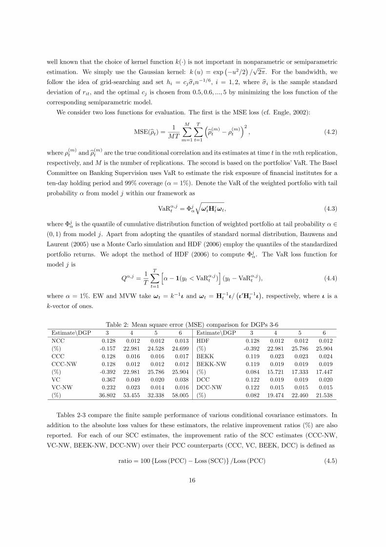
well known that the choice of kernel function k(·) is not important in nonparametric or semiparametricestimation. We simply use the Gaussian kernel: k (u) = exp
¡−u2/2
¢/√2π. For the bandwidth, we
follow the idea of grid-searching and set hi = cjbσin−1/6, i = 1, 2, where bσi is the sample standarddeviation of rit, and the optimal cj is chosen from 0.5, 0.6, ..., 5 by minimizing the loss function of the
corresponding semiparametric model.
We consider two loss functions for evaluation. The first is the MSE loss (cf. Engle, 2002):
MSE(bρt) = 1
MT
MXm=1
TXt=1
³bρ(m)t − ρ(m)t
´2, (4.2)
where ρ(m)t and bρ(m)t are the true conditional correlation and its estimates at time t in themth replication,
respectively, andM is the number of replications. The second is based on the portfolios’ VaR. The Basel
Committee on Banking Supervision uses VaR to estimate the risk exposure of financial institutes for a
ten-day holding period and 99% coverage (α = 1%). Denote the VaR of the weighted portfolio with tail
probability α from model j within our framework as
VaRα,jt = Φjα
qω0tH
j
tωt, (4.3)
where Φjα is the quantile of cumulative distribution function of weighted portfolio at tail probability α ∈(0, 1) from model j. Apart from adopting the quantiles of standard normal distribution, Bauwens and
Laurent (2005) use a Monte Carlo simulation and HDF (2006) employ the quantiles of the standardized
portfolio returns. We adopt the method of HDF (2006) to compute Φjα. The VaR loss function for
model j is
Qα,j =1
T
TXt=1
hα− 1(yt < VaRα,jt )
i(yt −VaRα,jt ), (4.4)
where α = 1%. EW and MVW take ωt = k−1ι and ωt = H−1t ι/¡ι0H−1t ι
¢, respectively, where ι is a
k-vector of ones.
Table 2: Mean square error (MSE) comparison for DGPs 3-6Estimate\DGP 3 4 5 6 Estimate\DGP 3 4 5 6NCC 0.128 0.012 0.012 0.013 HDF 0.128 0.012 0.012 0.012(%) -0.157 22.981 24.528 24.699 (%) -0.392 22.981 25.786 25.904CCC 0.128 0.016 0.016 0.017 BEKK 0.119 0.023 0.023 0.024CCC-NW 0.128 0.012 0.012 0.012 BEKK-NW 0.119 0.019 0.019 0.019(%) -0.392 22.981 25.786 25.904 (%) 0.084 15.721 17.333 17.447VC 0.367 0.049 0.020 0.038 DCC 0.122 0.019 0.019 0.020VC-NW 0.232 0.023 0.014 0.016 DCC-NW 0.122 0.015 0.015 0.015(%) 36.802 53.455 32.338 58.005 (%) 0.082 19.474 22.460 21.538
Tables 2-3 compare the finite sample performance of various conditional covariance estimators. In
addition to the absolute loss values for these estimators, the relative improvement ratios (%) are also
reported. For each of our SCC estimates, the improvement ratio of the SCC estimates (CCC-NW,
VC-NW, BEEK-NW, DCC-NW) over their PCC counterparts (CCC, VC, BEEK, DCC) is defined as
ratio = 100 Loss (PCC)− Loss (SCC) /Loss (PCC) (4.5)
16

Table 3: Value-at-Risk (VaR) loss comparison for DGPs 3-6EW MVW
Estimate\DGP 3 4 5 6 3 4 5 6NCC 0.082 0.075 0.069 0.061 0.033 0.034 0.033 0.035(%) 2.038 0.399 -0.146 6.769 29.892 27.015 23.148 24.086HDF 0.083 0.075 0.069 0.065 0.044 0.042 0.037 0.042(%) 0.000 -0.133 0.000 0.615 5.806 9.368 15.509 9.462CCC 0.083 0.075 0.069 0.065 0.047 0.046 0.043 0.047CCC-NW 0.081 0.074 0.068 0.060 0.031 0.033 0.032 0.034(%) 2.638 1.332 0.729 8.154 33.118 29.194 25.000 27.527VC 0.328 0.085 0.069 0.067 0.297 0.060 0.043 0.050VC-NW 0.079 0.074 0.068 0.060 0.084 0.036 0.032 0.034(%) 76.031 13.130 0.729 10.912 71.698 40.168 25.463 33.135BEKK 0.083 0.076 0.069 0.066 0.047 0.046 0.043 0.047BEKK-NW 0.081 0.074 0.069 0.060 0.031 0.033 0.032 0.034(%) 2.521 2.243 0.291 8.092 32.976 28.913 24.651 27.350DCC 0.083 0.075 0.068 0.065 0.046 0.046 0.043 0.046DCC-NW 0.081 0.074 0.068 0.060 0.031 0.032 0.032 0.034(%) 2.292 1.198 0.731 8.308 33.045 29.258 24.942 27.586
where Loss(SCC) and Loss(PCC) are the MSE or VaR loss for the SCC estimate and the start-up PCC
estimate, respectively. Since the NCC models have no start-up parametric model, we compare them
with the parametric CCC estimate. For the HDF estimator, we take the parametric CCC model as
the start-up model. Positive value of improvement ratio means better performance of SCC estimators
than their start-up PCC estimators or NCC/HDF estimators than the parametric CCC estimators. We
summarize some interesting findings below. First, in terms of MSE, our SCC estimates usually beat
the start-up PCC estimates except for the CCC estimate in DGP 3. Second, regardless of portfolio
weighting methods, our SCC estimates always demonstrate better performance than the corresponding
PCC estimates in terms of VaR loss. Third, we observe higher VaR loss improvement ratio of the SCC
estimate over its start-up PCC estimate in MVW portfolio than in EW portfolio across nearly all DGPs.
The only exception is the improvement ratio of the VC-NW estimate over the parametric VC estimate
in DGP 3: the ratio for the VaR loss of EW portfolio is 76.03%, higher than that of MVW portfolio,
71.70%. Fourth, regarding MSE, the superiority ranking of semiparametric estimators is not always
the same as that of parametric estimators. In DGP 5, for instance, the performance of the parametric
estimators in the CCC, DCC, BEKK and VC models deteriorates in order, while the deteriorating order
of their semiparametric counterparts is the CCC-NW, VC-NW, DCC-NW and BEKK-NW models.
4.2 Empirical Analysis
We examine three sets of financial daily time series data, the Dow Jones Industrial Average Index
and Standard & Poor’s 500 Index (DJIA&SPX) from January 2, 2003 to December 31, 2007 (T =
1258 observations); Cotation Assistée en Continu 40 and Financial Times Stock Exchange 100 Index
(CAC&FTSE) from January 2, 2003 to December 31, 2007 (T = 1281 observations); and Hang Seng
Index and Straits Times Index (HSI&STI) from January 2, 2003 to December 31, 2007 (T = 1260
17

observations). All data sets are downloaded from Yahoo Finance. For the ease of interpretation, we
compute the percentage returns (rt) as log returns multiplied by 100 and then demeaned. We split
the whole samples at day R, the last day of 2006, use samples from 2003 to 2006 for in-sample (IS
hereafter) estimation, and apply the “fixed scheme” to do one-day-ahead conditional covariance matrix
forecast throughout end of year 2007. The IS standardized residuals are sorted to compute the p-value
for VaR calculation later. “Fixed scheme” means in the whole forecasting period we keep using the same
parameters, whose estimation is based on information set FR. For the out-of-sample (OoS hereafter)forecasting, the forecast length is 251, 255, and 250 days for the three data sets, respectively.
For each series, we assume the conditional mean is zero based on efficient market hypothesis. When
implementing our nonparametric test for the correct specification of PCC model based on the stan-
dardized residuals from the IS estimation, we choose the kernel and bandwidth as in Section 4.1.2. We
choose the conditioning variable xt as the one-day lagged percentage return, i.e., xt = rt−1.We conduct
our nonparametric test for the three data sets and reject the null of correct specification of all the four
PCC models under investigation at the 1% level. In view of this evidence we apply our SCC models to
capture the remaining information in the standardized residuals of various PCC models.
When applying SCC models to these empirical data sets, we choose the kernel function and band-
width as in Section 4.1.3. The conditioning variable is set as the one-day lagged percentage return,
i.e., xt = rt−1. To judge the relative fitting and predictive ability of various conditional covariance
models, we modify the two types of criterion functions used in Section 4.1.3. The MSE criterion in
(4.2) can not be used here because the true conditional covariance matrix is not observable. Zangari
(1997) addresses the advantage of focusing on the volatility hyt of the aggregate portfolio yt ≡ ω0rt
instead of the conditional covariance matrix Ht, where hyt = ω0Htω and ω is a weight vector. When
comparing the predictability of univariate GARCH models, Awartani and Corradi (2005) substitute the
unobservable volatility by the squared observed returns because of the rank-preserving property of this
substitution under the MSE loss. They conclude that both squared returns and realized volatility are
good proxies of the unobservable volatility for the purposes of model comparisons. Because intraday
returns are not available, Pelletier (2006) suggests using the cross-product of daily returns instead of
cumulative cross-product of intraday returns over the forecast horizon. Following these authors, we
compare various models by calculating the predictive measures, MSEjOoS for model j, as
MSEjOoS =1
(T −R)
T−1Xt=R
³ω0t+1 bHj
t+1ωt+1 − ω0t+1rt+1r0t+1ωt+1
´2, (4.6)
where bHj
t+1 is the one-step-ahead forecaster of Ht+1 at time t from model j. The second loss is modified
from VaR loss (4.3) in simulations:
Qα,jOoS =
1
(T −R)
T−1Xt=R
hα− 1(yt+1 < VaRα,jOoS,t+1)
i(yt+1 −VaRα,jOoS,t+1), (4.7)
where VaRα,jOoS,t+1 = Φjα
qω0t+1
bHj
t+1ωt+1, Φjα is the quantiles of the standardized IS portfolio returns,
and α = 1%. The in-sample (IS) losses are similarly defined.
The IS and OoS performance measures of different conditional covariance models over these empir-
ical data sets are presented in Tables 4-5. For each pair of parametric start-up PCC model and the
18

Table 4: MSE loss for equal weight and minimum variance weight portfoliosDJIA&SPX CAC&FTSE HSI&STI DJIA&SPX CAC&FTSE HSI&STIIS OoS IS OoS IS OoS IS OoS IS OoS IS OoS
EW MVWNCC 1.44 3.05 1.65 3.77 1.48 14.60 0.66 2.45 0.86 5.09 1.14 13.78% 15.30 -5.43 55.76 -7.51 14.71 -13.84 37.74 -7.30 73.19 -49.22 32.11 -26.25HDF 1.31 2.87 1.85 3.41 1.41 12.60 0.63 2.27 1.12 3.36 1.07 10.31% 23.16 0.73 50.62 2.92 18.49 1.80 39.87 0.55 65.09 1.55 35.97 5.62CCC 1.70 2.89 3.74 3.50 1.74 12.83 1.05 2.28 3.21 3.41 1.68 10.93CCC-NW 1.31 2.87 1.93 3.39 1.41 12.58 0.63 2.27 1.26 3.36 1.05 10.56% 23.05 0.77 48.30 3.01 18.80 1.91 40.29 0.53 60.70 1.45 37.12 3.36VC 1.70 2.89 3.75 3.50 1.74 12.74 1.05 2.30 3.18 3.42 1.68 10.74VC-NW 1.31 2.87 1.85 3.39 1.41 12.52 0.62 2.28 1.13 3.36 1.05 10.18% 23.02 0.74 50.69 2.90 18.65 1.74 41.18 0.87 64.38 1.88 37.41 5.20BEKK 1.71 2.89 3.82 3.54 1.74 12.76 1.07 2.29 2.92 3.83 1.68 10.81BEKK-NW 1.31 2.87 1.67 3.43 1.42 12.56 0.62 2.26 0.93 3.62 1.05 10.76% 23.02 0.45 56.23 2.95 18.34 1.61 42.46 1.20 68.42 5.96 37.16 0.47DCC 1.70 2.89 3.74 3.50 1.74 12.72 1.03 2.30 3.14 3.45 1.69 11.22DCC-NW 1.31 2.86 1.67 3.40 1.42 12.46 0.60 2.28 0.93 3.35 1.06 10.02% 23.07 0.73 55.52 2.89 18.46 2.03 41.79 0.97 70.79 2.74 37.29 10.72
corresponding SCC model, the improvement ratio is reported in percentage as before. For NCC and
HDF models, we report the absolute loss values and the improvement ratio relative to the CCC model.
We summarize some interesting findings below. First, for both loss functions, our semiparametric model
can always reduce the IS loss values of the start-up parametric model no matter which weight to use.
Second, in terms of MSE, the improvement ratio of our SCC model against the start-up PCC model is
always positive for both IS and OoS evaluations, both EW and MVW portfolios, and all data sets under
examination. The same MSE superior pattern is observed in HDF which produces positive improvement
ratio over CCC model across data sets and sample period. But this supporting evidence is not found for
the NCC model. But the relative out-of-sample gains of our and HDF’s semiparametric estimators over
the parametric estimators are generally much smaller than the relative in-sample gains. We conjecture
that one of the reason for this is the use of fixed-scheme (instead of rolling-window) forecast. Third,
for DJIA&SPX and CAC&FTSE MVW portfolios, our SCC model can always reduce the VaR losses
no matter which sample period (IS or OoS) or which start-up parametric model we choose. We do not
observe the same phenomena for HSI&STI data, which might be explained by their emerging market
properties. Fourth, there exists no semiparametric model that is universally the best across different
data sets, weighting schemes or loss functions. While the SBEKK-NW model has the smallest OoS
VaR loss across the weighting methods for DJIA&SPX portfolio, its OoS MSE is bigger than that of
the CCC-NW, VC-NW and DCC-NW models for the equal weight DJIA&SPX portfolio. Last, for the
same conditional covariance model, the MVW portfolio always outperforms the EW portfolio in terms
of IS losses and generally outperforms the latter in terms of OoS losses.
19

Table 5: VaR loss for equal weight and minimum variance portfoliosDJIA&SPX CAC&FTSE HSI&STI DJIA&SPX CAC&FTSE HSI&STIIS OoS IS OoS IS OoS IS OoS IS OoS IS OoS
EW MVWNCC 0.030 0.071 0.034 0.056 0.031 0.117 0.021 0.032 0.025 0.046 0.025 0.112% -3.44 -25.53 -5.538 -12.85 4.012 -70.36 12.03 19.30 2.703 -4.56 20.38 -94.12HDF 0.025 0.057 0.031 0.050 0.029 0.063 0.021 0.039 0.023 0.042 0.024 0.058% 13.40 0.176 6.154 0.402 10.49 8.029 12.03 3.258 10.81 4.100 22.93 -1.038CCC 0.029 0.057 0.033 0.050 0.032 0.069 0.024 0.040 0.026 0.044 0.031 0.058CCC-NW 0.025 0.057 0.031 0.050 0.029 0.063 0.021 0.039 0.023 0.042 0.024 0.058% 12.72 0.000 5.846 0.402 10.19 7.737 12.03 3.008 10.81 3.872 24.52 -0.519VC 0.029 0.057 0.033 0.049 0.032 0.062 0.025 0.041 0.027 0.038 0.031 0.054VC-NW 0.025 0.056 0.031 0.049 0.029 0.058 0.021 0.040 0.024 0.037 0.024 0.056% 13.61 0.704 6.422 0.406 8.438 6.431 15.10 1.478 12.22 1.583 24.20 -4.664BEKK 0.029 0.054 0.035 0.051 0.032 0.059 0.025 0.038 0.028 0.036 0.031 0.060BEKK-NW 0.025 0.054 0.031 0.051 0.030 0.057 0.021 0.038 0.024 0.035 0.024 0.059% 14.04 0.370 10.951 0.000 4.444 2.381 17.06 0.262 12.33 2.493 24.04 1.656DCC 0.029 0.057 0.033 0.049 0.032 0.062 0.025 0.041 0.027 0.037 0.032 0.054DCC-NW 0.025 0.056 0.030 0.049 0.029 0.059 0.021 0.041 0.024 0.036 0.024 0.054% 13.36 0.885 7.034 0.000 9.091 4.693 14.23 0.735 11.28 3.784 25.32 0.924
ACKNOWLEDGEMENTS
The authors gratefully thank Serena Ng, the associate editor, and an anonymous referee for their
many insightful comments that have led great improvement of the presentation. The authors also thank
the conference and seminar participants at the Far Eastern and South Asian Meeting of the Econometric
Society (2008), the Australasian Meeting of Econometric Society (2006), Catholic University of Louvain,
European FMA conference (2005), Forum of Interdisciplinary Mathematics (FIM) Portugal, Indiana
University, University of Cambridge, and University of Oxford for their comments. All errors are the
authors’ responsibilities. The second author gratefully acknowledges the financial support from the
NSFC under the grant numbers 70501001 and 70601001. The third author acknowledges the financial
support from the academic senate, UCR.
Appendix
A Proof of the Main Results
We use C to signify a generic constant whose exact value may vary from case to case, and a0 to denote
the transpose of a. Let bf (x) = T−1PT
s=1Kh(xs − x), and
eGnp (x) = T−1TXs=1
ese0sKh(xs − x)/ bf (x) .
The following two lemmas are needed for the proof of Theorem 3.1.
20
Lemma A.1 Under Assumptions A1-A7,
√Th!
nvech
³eGnp (x)´− vech (Gnp (x))− vech (B (x))
od→ N
¡0, μq02f(x)
−1D+k Ω (x)D
+0k
¢,
where recall h!=h1...hq, and Ω (x) and B (x) are defined in Theorem 3.1.
Proof. Let WTijs = Kh(xs −x)eisejs and WTij = T−1PT
s=1WTijs, where eis is the ith element of
es. Define two k (k + 1) /2−vectors:
WTs = (WT11s,WT21s, ...,WTk1s,WT22s, ...,WTk2s, ...,WTkks)0
WT = (WT11,WT21, ...,WTk1,WT22, ...,WTk2, ...,WTkk)0.
Clearly, WT = T−1PT
s=1WTs. The statistic WTij/ bf (x) estimates the (i, j)th element of Gnp (x) by
using the pseudo-data et,xt . Let ZTs = (h!/T )1/2 (WTs −E (WTs)) and ZT =PT
s=1 ZTs. Write
WT = T−1TXs=1
E (WTs) + T−1TXs=1
(WTs −E (WTs))
= T−1TXs=1
E (WTs) + (Th!)−1/2
TXs=1
ZTs
The first term contributes to the bias of eGnp (x) whereas the second term contributes to the variance
of eGnp (x) . The proof will be completed by proving the following claims:
bf (x) p→ f (x) , (A.1)
T−1TXs=1
E (WTs) = f (x) vech (Gnp (x)) + f (x) vech (B (x)) + oP (khk2), (A.2)
and
ZT =TXs=1
ZTsd→ N
¡0, μq02f (x)D
+k Ω (x)D
+0k
¢. (A.3)
(A.1) follows from standard results in kernel density estimation. Using standard arguments for
analyzing the bias of the Nadaraya-Watson estimator, we have
E (WTijs) = E [Kh(xs − x)eitejt] = f (x) [Gnp,ij (x) +Bij (x)] + oP (khk2)
where
Bij (x) =μ212f (x)
qXl=1
∙2∂f (x)
∂xl
∂Gnp,ij (x)
∂xl+ f (x)
∂2Gnp,ij (x)
∂xl∂xl
¸h2l .
Thus (A.2) follows by the stationarity assumption. To show (A.3), let c = (c11, c21..., ck1, c22, ..., ck2, ..., ckk)0
denote a k (k + 1) /2-vector of bounded constants such that kck = 1. By the Cramér-Wold device, it
suffices to show
c0ZT =TXs=1
c0ZTsd→ N
¡0, μq02f (x) c
0D+k Ω (x)D
+0k c¢. (A.4)
21

By construction, E (ZT ) = 0, and
Var (c0ZT ) = T−1h!TXt=1
Var (c0WTt) + 2T−1h!
XX1≤s<t≤T
Cov (c0WTs, c0WTt) ≡ A1 +A2. (A.5)
We calculate A1 and A2 in turn.
A1 = T−1h!TXt=1
Var (c0WTt)
=XX1≤j≤i≤k
XX1≤m≤l≤k
cijclm
"T−1h!
TXt=1
E£K2h(xt − x)Cov
¡ij,t, lm,t|xt = x
¢¤#= μq02f (x)
XX1≤j≤i≤k
XX1≤m≤l≤k
cijclmωij,lm (x) +O (khk)
= μq02f (x) c0D+
k Ω (x)D+0k c+O (khk) , (A.6)
where ij,t = eitejt and ωij,lm (x) =Cov¡
ij,t, lm,t|xt = x¢. To calculate A2, write
A2 = 2T−1h!XX1≤s<t≤T
XX1≤j≤i≤k
XX1≤m≤l≤k
cijclmCov (WTijs,WTlmt)
= 2h!TXt=2
µ1− j
T
¶XX1≤j≤i≤k
XX1≤m≤l≤k
cijclmCov (WTij1,WTlmt) . (A.7)
Noting that even though vt is a m.d.s., this does not ensure that Cov(WTijs,WTlmt) = 0 for s 6= t.
To bound the right hand side of (A.7), we split it into two terms as follows
TXt=2
|Cov (WTij1,WTlmt)| =dTXt=2
|Cov (WTij1,WTlmt)|+TX
t=dT+1
|Cov (WTij1,WTlmt)| ≡ J1 + J2, (A.8)
where dT is a sequence of positive integers such that dTh! → 0 as T → ∞. Since for any t >
1, |E (WTij1WTlmt)| = O (1) ,
J1 = O (dn) . (A.9)
For J2, by the Davydov’s inequality (e.g., Bosq, 1996, p.19), we have
|Cov (WTij1WTlmt)| ≤ C [α (t− 1)]δ/(2+δ) supi,j
³E |WTij1|2+δ
´2/(2+δ)≤ C (h!)
−(2+2δ)/(2+δ)[α (t− 1)]δ/(2+δ) .
So by Assumption A1,
J2 ≤ C (h!)−(2+2δ)/(2+δ)TX
t=dT+1
[α (t− 1)]δ/(2+δ)
≤ C (h!)−(2+2δ)/(2+δ) d−aT
∞Xt=dT
ta [α (t)]δ/(2+δ) = o³(h!)−1
´, (A.10)
by choosing dT such that daT (h!)δ/(2+δ) → ∞. The last condition can be simultaneously met with
dTh! → 0 for a well chosen sequence dT because a > δ/ (2 + δ) by Assumptions A1 and A7. (A.7)-
(A.10) imply that
A2 = O (dnh!) + o (1) = o (1) .
22

Hence,
Var (c0ZT ) = μq02f (x) c0D+
k Ω (x)D+0k c+ o (1) .
Using the standard Doob’s small-block and large-block technique, we can finish the rest of the
normality proof of (A.4) by following the arguments of Cai, Fan and Yao (2000, pp. 954-955). ¥
Lemma A.2 Under Assumptions A1-A7,
vech³bGnp (x)
´− vech
³eGnp (x)´= oP
³(Th!)−1/2
´.
Proof. Let∆ (x) = [vec( bGnp (x))−vec( eGnp (x))] bf (x) .Noting that bf (x) p→ f (x) > 0 and vech(A) =
D+k vec(A) for any symmetric k × k matrix A, it suffices to show that ∆ (x) = oP ((Th!)
−1/2). By the
first order Taylor expansion,
bet = et(bθ) = H−1/2p,t
³bθ´ rt = et + ξt¡θ¢ ³bθ − θ∗
´(A.11)
where recall ξt (θ) = ∂et(θ)/∂θ0, and θ lies between bθ and θ∗. By Assumptions A2-A3, θ
p→ θ∗. So
∆ (x) =1
T
TXt=1
Kh(xt − x)vec [betbe0t − ete0t]=
1
T
TXt=1
Kh(xt − x)vec∙ξt¡θ¢ ³bθ − θ∗
´³bθ − θ∗´0ξt¡θ¢0¸
+2
T
TXt=1
Kh(xt − x)vec∙et
³bθ − θ∗´0ξt¡θ¢0¸
=1
T
TXt=1
Kh(xt − x)¡ξt¡θ¢⊗ ξt
¡θ¢¢vec
∙³bθ − θ∗´³bθ − θ∗
´0¸
+2
T
TXt=1
Kh(xt − x)¡ξt¡θ¢⊗ et
¢ ³bθ − θ∗´
≡ ∆1 (x) + 2∆2 (x) .
By the triangle inequality, Markov inequality, and Assumptions A4-A7,
k∆1 (x)k ≤ 1
T
TXt=1
Kh(xt − x)°°°°¡ξt ¡θ¢⊗ ξt ¡θ¢¢ vec ∙³bθ − θ∗
´³bθ − θ∗´0¸°°°°
≤ 1
T
TXt=1
Kh(xt − x)°°ξt ¡θ¢°°2 °°°bθ − θ∗
°°°2≤ 1
T
TXt=1
Kh(xt − x)D2
t
°°°bθ − θ∗
°°°2 = OP
µ1
Th!
¶,
and
k∆2 (x)k ≤ 1
T
TXt=1
Kh(xt − x)°°°¡ξt ¡θ¢⊗ et¢ ³bθ − θ∗
´°°°≤ 1
T
TXt=1
Kh(xt − x)°°ξt ¡θ¢°° ketk°°°bθ − θ∗
°°°23

≤ 1
T
TXt=1
Kh(xt − x)Dt ketk°°°bθ − θ∗
°°° = OP
³T−1/2
´.
Consequently, ∆ (x) = OP ((Th!)−1 + T−1/2) = oP ((Th!)
−1/2).¥
Proof of Theorem 3.1
The result follows from Lemmas A.1-A.2.¥
Proof of Corollary 3.2
By Assumptions A3-A5, bHp,t = H1/2p,t (
bθ) = H1/2p,t + oP (1) . By Theorem 3.1, bGnp,t = bGnp (xt) =
Gnp,t + oP (1) . It follows from the Slutsky theorem that
bHsp,t = bH1/2p,tbGnp,t
bH1/2p,t =H
1/2p,t Gnp,tH
1/2p,t + oP (1) = Ht + oP (1) ,
and bH∗sp,t =H∗t + oP (1) , where H∗t is a diagonal matrix with the square roots of the diagonal elements
of Ht on its diagonal. Hence bRsp,t =³bH∗sp,t´−1 bHsp,t
³bH∗sp,t´−1 p→ (H∗t )−1Ht (H
∗t )−1 = Rt.
To show (ii), noting that by Assumptions A3-A5,
bHsp,t −Ht = bH1/2p,tbGnp,t
bH1/2p,t −H
1/2p,t Gnp (xt)H
1/2p,t
= H1/2p,t
³bGnp (xt)−Gnp (xt)´H1/2p,t +
n³bH1/2p,t −H
1/2p,t
´ bGnp,t
³bH1/2p,t −H
1/2p,t
´+³bH1/2
p,t −H1/2p,t
´ bGnp,tH1/2p,t +H
1/2p,tbGnp,t
³bH1/2p,t −H
1/2p,t
´o= H
1/2p,t
³bGnp (xt)−Gnp (xt)´H1/2p,t +Op
³T−1/2
´,
we have
√Th!
hvech
³bHsp,t
´− vech (Ht)
i=√Th!D+
k
hvec
³bHsp,t
´− vec (Ht)
i=√Th!D+
k vec³H1/2p,t
³bGnp (xt)−Gnp (xt)´H1/2p,t
´+ oP (1)
=√Th!D+
k
³H1/2p,t ⊗H
1/2p,t
´vec
³bGnp (xt)−Gnp (xt)´+ oP (1)
=√Th!D+
k
³H1/2p,t ⊗H
1/2p,t
´Dkvech
³bGnp (xt)−Gnp (xt)´+ oP (1) .
Then by Theorem 3.1,
√Th!
hvech
³bHsp,t
´− vech (Ht)−Bt (xt)
id→MN
³0, μq02f(xt)
−1Ωt (x)´,
where
Bt (x) = D+k
³H1/2p,t ⊗H
1/2p,t
´Dkvech (B (x)) = D+
k
³H1/2p,t ⊗H
1/2p,t
´vec (B (x))
= D+k vec
³H1/2p,t B (x)H
1/2p,t
´= vech
³H1/2p,t B (x)H
1/2p,t
´by the definitions of vech, vec, Dk, and D+
k and the fact that (A⊗A)vec(B (x)) =vec(AB (x)A) for
24

any k × k matrix A, and
Ωt (x) = D+k
³H1/2p,t ⊗H
1/2p,t
´DkD
+k Ω (x)D
+0k D0
k
³H1/2p,t ⊗H
1/2p,t
´ ¡D+k
¢0= D+
k Nk
³H1/2p,t ⊗H
1/2p,t
´Ω (x)
³H1/2p,t ⊗H
1/2p,t
´Nk
¡D+k
¢0= D+
k
³H1/2p,t ⊗H
1/2p,t
´Ω (x)
³H1/2p,t ⊗H
1/2p,t
´ ¡D+k
¢0= D+
k Ωt (x)¡D+k
¢0by the fact that Nk ≡ DkD
+k is symmetric, NkDk = Dk, NkD
+0k = D+0
k , and Nk(A⊗A) = (A⊗A)Nk
for any k × k matrix A. ¥
Proof of Theorem 3.3
Let ιi denote a k × 1 vector that has 1 in the ith row and 0 elsewhere. Then
beit = ι0ibet = ι0i bH−1/2p,t rt = ι0iH−1/2p,t rt + ι0i
³bH−1/2p,t −H−1/2p,t
´rt = eit + νit,
where νit = ι0i
³bH−1/2p,t −H−1/2p,t
´rt. Note that for notational simplicity we have suppressed the depen-
dence of νit on the sample size T. It follows that
1
T
TXt=1
(beitbejt − δij)Kh (xt − x) =1
T
TXt=1
[(eit + νjt) (eit + νjt)− δij ]Kh (xt − x) =4Xl=1
Aij,l (x) ,
and1
T 2
TXt=1
(beitbejt − δij)2Kh (0) =
1
T
TXt=1
[(eit + νit) (ejt + νjt)− δij ]2Kh (0) =
4Xl=1
Bij,l,
where
Aij,1 (x) =1T
PTt=1 (eitejt − δij)Kh (xt − x) , Bij,1 =
1T
PTt=1 (eitejt − δij)
2Kh (0) ,
Aij,2 (x) =1T
PTt=1 νitνjtKh (xt − x) , Bij,2 =
1T
PTt=1 ν
2itν
2jtKh (0) ,
Aij,3 (x) =1T
PTt=1 eitνjtKh (xt − x) , Bij,3 =
1T
PTt=1 e
2itν
2jtKh (0) ,
Aij,4 (x) =1T
PTt=1 ejtνitKh (xt − x) , Bij,4 =
1T
PTt=1 e
2jtν
2itKh (0) .
Consequently,
bΓ =k−1Xi=1
kXj=i
Z "1
T
TXt=1
(beitbejt − δij)Kh (xt − x)#2
dx− 1
T 2
k−1Xi=1
kXj=i
TXt=1
(beitbejt − δij)2Kh (0)
=k−1Xi=1
kXj=i
("Z 4Xl=1
A2ij,l (x) + 2Aij,1 (x)Aij,2 (x) + 2Aij,1 (x)Aij,3 (x) + 2Aij,1 (x)Aij,4 (x)
+2Aij,2 (x)Aij,3 (x) + 2Aij,2 (x)Aij,4 (x) + 2Aij,3 (x)Aij,4 (x)
¸dx−
4Xl=1
Bij,l
).
Then we can write T (h!)1/2 bΓ =P10l=1 ClT , where
ClT = T (h!)1/2k−1Xi=1
kXj=i
½ZA2ij,l (x) dx−Bij,l
¾for l = 1, 2, 3, 4,
ClT = T (h!)1/2
k−1Xi=1
kXj=i
ZAij,1 (x)Aij,l−3 (x) dx for l = 5, 6, 7,
25

ClT = T (h!)1/2k−1Xi=1
kXj=i
ZAij,2 (x)Aij,l−5 (x) dx for l = 8, 9, and
C10T = T (h!)1/2
k−1Xi=1
kXj=i
ZAij,3 (x)Aij,4 (x) dx.
The proof will be completed if we can show C1Td→ N
¡0, σ20
¢, and ClT = oP (1) for l = 2, 3, · · · , 10. We
only prove C1Td→ N
¡0, σ20
¢and ClT = oP (1) for l = 2, 3, 5 since the other cases are similar.
We first show that C1Td→ N
¡0, σ20
¢. Let ςt = (x0t, e
0t)0 and φ (ςt, ςs) = (h!)
1/2Pk−1i=1
Pkj=i(eitejt −
δij) (eisejs− δij) Kh (xt − xs) .We can write C1T = 2T−1P
1≤t<s≤T φ (ςt, ςs) , which is a second order
U-statistic and is degenerate under the null. Under Assumptions A1, A4, and A6-A9 and the null
hypothesis, one can verify the conditions of Lemma B.1 in Gao and King (2003) are satisfied so that a
central limit theorem applies to C1T . The asymptotic variance is given by limn→∞ 2E[φ (ςt, ςt)2] = σ20,
where ςt is an independent copy of ςt.
To show C2T = oP (1) , write
C2T = T−1 (h!)1/2k−1Xi=1
kXj=i
TXs=1
TXt6=s
νisνjsνitνjtKh (xt − xs) .
By (A.11) and Assumption A5, |νit| = |ι0i(bet − et)| = |ι0iξt(θ)(bθ − θ∗)| ≤ Dt||bθ − θ∗||, where recallξt (θ) = ∂et(θ)/∂θ
0 and θ lies between bθ and θ∗. By Assumptions A5 and A3,
|C2T | ≤k (k + 1)
2T−1 (h!)1/2
TXs=1
TXt6=s
D2
tD2
sKh (xt − xs)°°°bθ − θ∗
°°°4= Op(T (h!)
1/2)Op
¡T−2
¢= oP (1) ,
where the second line follows from a simple application of the Markov inequality, and the fact that for
t 6= s
EhD2
tD2
sKh (xt − xs)i≤nEhD4
tKh (xt − xs)io1/2 n
EhD4
sKh (xt − xs)io1/2
= O (1) .
Similarly, noting that C3T = T−1 (h!)1/2Pk−1
i=1
Pkj=i
PTs=1
PTt6=s eitνjteisνjsKh (xt − xs) , we have,
|C3T | ≤k (k + 1)
2T−1 (h!)1/2
¯¯TXs=1
TXt=1
ketk keskDtDsKh (xt − xs)¯¯ °°°bθ − θ∗
°°°2= Op(T (h!)
1/2)Op
¡T−1
¢= oP (1) .
Noting that C5T = T−1 (h!)1/2Pk−1
i=1
Pkj=i
PTs=1
PTt=1 (eisejs − δij) νitνjtKh (xt − xs) , we can write
C5T = C5T,a + C5T,b, where
C5T,a = T−1 (h!)1/2k−1Xi=1
kXj=i
TXs=1
TXt6=s
(eisejs − δij) νitνjtKh (xt − xs) , and
C5T,b = T−1 (h!)1/2k−1Xi=1
kXj=i
TXt=1
(eitejt − δij) νitνjtKh (0) .
26

By Assumptions A3, A5 and A8, and the Markov inequality,
|C5T,a| ≤k (k + 1)
2T−1 (h!)1/2
TXs=1
TXt6=s
³kesk2 + 1
´D2
tKh (xt − xs)°°°bθ − θ∗
°°°2= Op(T (h!)
1/2)Op
¡T−1
¢= oP (1) ,
and
|C5T,b| ≤k (k + 1)
2T−1 (h!)1/2
TXt=1
³ketk2 + 1
´D2tKh (0)
°°°bθ − θ∗
°°°2= Op((h!)
−1/2)Op
¡T−1
¢= oP (1) ,
Consequently, C5T = oP (1) . This concludes the proof of the theorem.¥
Proof of Theorem 3.4
Under H1(T−1/2 (h!)−1/4), the expression T (h!)1/2 bΓ =P10
l=1ClT obtained in the proof of Theorem
3.3 continues to hold. In addition, one can verify that under H1(T−1/2 (h!)−1/4), ClT = oP (1) continues
to hold for l = 2, 3, · · · , 10. The main change is associated with the term C1T . Let ijt = eitejt − δij .
Let Et ( ijt) denote the conditional expectation of ijt given Ft−1 and ijt = ijt − Et ( ijt). Then we
can write C1T = C1T,a + C1T,b + C1T,c, where
C1T,a = T−1 (h!)1/2k−1Xi=1
kXj=i
TXs=1
TXt6=s
ijs ijtKh (xt − xs) ,
C1T,b = T−1 (h!)1/2k−1Xi=1
kXj=i
TXs=1
TXt6=s
Es ( ijs)Et ( ijt)Kh (xt − xs) , and
C1T,c = 2T−1 (h!)1/2k−1Xi=1
kXj=i
TXs=1
TXt6=s
ijsEt ( ijt)Kh (xt − xs) .
C1T,a now plays the role of C1T in the proof of Theorem 3.3, and we can show that C1T,ad→ N
¡0, σ20
¢.
Next, noting that under H1(T−1/2 (h!)−1/4), Et ( ijt) = T−1/2 (h!)−1/4∆ij (xt) , we have
C1T,b = T−2k−1Xi=1
kXj=i
TXs=1
TXt6=s∆ij (xs)∆ij (xt)Kh (xt − xs)
=T − 1T
2
T (T − 1)X
1≤t<s≤Tϕ (xt,xs) ≡
T − 1T
eC1T,b (A.12)
where ϕ (xt,xs) =Pk−1
i=1
Pkj=i∆ij (xs)∆ij (xt)Kh (xt − xs) . Noticing that eC1T,b is a second order U-
statistic, a typical WLLN for U-statistic of strong mixing process (e.g., Borovkova, Burton, and Dehling,
1999) would require that ϕ (xt,xs) : t, s ≥ 1, t 6= s be uniformly integrable, which is difficult to verifyhere. By the H-decomposition, we can write
eC1T,b = ϑT + 2H(1)T +H
(2)T , (A.13)
where ϑT =R R
ϕ (xt,xs) f (xt) f (xs) dxtdxs, H(1)T = 1
T
PTt=1 ϕ1 (xt) − ϑT , H
(2)T = 2
T (T−1)P
1≤t<s≤Tϕ (xt,xs) , ϕ1 (xt) =
Rϕ (xt,xs) f (xs) dxs, and ϕ (xt,xs) = ϕ (xt,xs)− ϕ1 (xt)− ϕ1 (xs) + ϑT . By the
27

Fubini theorem and the change of variables, we have
ϑT =k−1Xi=1
kXj=i
Z Z∆ij (xs)∆ij (xt)Kh (xt − xs) f (xt) f (xs) dxtdxs
=k−1Xi=1
kXj=i
Z∆2ij (x) f
2 (x) dx+ o (1) . (A.14)
Note that ϕ1 (xt) is a measurable function of xt and inherits the α-mixing property of the latter. By
Assumption A1, ϕ1 (xt) is a strictly stationary α-mixing process with mixing coefficient α (j) → 0 as
j → ∞. By Proposition 3.44 of White (2001), ςt is also ergodic. Furthermore, it is easy to verify that
E |ϕ1 (xt)| <∞. It follows from the Ergodic theorem (e.g., White, 2001, Theorem 3.34) that
H(1)T
p→ 0. (A.15)
Now, H(2)T is a standard second order degenerate U-statistic with a symmetric kernel ϕ (.,. ) : ϕ (xt,xs) =
ϕ (xs,xt) and Eϕ (x1,a) = 0 for any nonrandom a ∈ Rq. Noting that
max1<t≤T
max
½E |ϕ (x1,xt)|2(1+δ) ,
Z|ϕ (x1,xt)|2(1+δ) dF (x1) dF (xt)
¾= O
³(h!)−(1+2δ)
´where F (.) is the distribution function of xt, it follows from Lemma C.2 of Gao and King (2003) that
EhH(2)T
i2≤ C
µ2
T (T − 1)
¶2T 2 (h!)
− 1+2δ1+δ = O
³T−2 (h!)−
1+2δ1+δ
´= o (1) .
Hence by the Chebyshev inequality
H(2)T = oP (1) . (A.16)
Combining (A.12)-(A.16) yields C1T,bp→Pk−1
i=1
Pkj=i
R∆2ij (x) f
2 (x) dx ≡ ∆0.Now, write C1T,c = C1T,c1+C1T,c2, where C1T,c1 = 2T−3/2 (h!)
1/4Pk−1i=1
Pkj=i
PT1≤t<s≤T ijs∆ij (xt)
Kh (xt − xs) and C1T,c2 = 2T−3/2 (h!)1/4Pk−1
i=1
Pkj=i
PT1≤s<t≤T ijs∆ij (xt)Kh (xt − xs) . By construc-
tion E ( ijs|Fs−1) = 0. It follows that E (C1T,c1) = 0 by the law of iterated expectations and the
hypothesis that (xt,xs) ∈ Fs−1 for t < s. By the Davydov’s inequality (e.g., Bosq, 1996, p.19), we have
E (C1T,c2) = 2T−3/2 (h!)1/4k−1Xi=1
kXj=i
TX1≤s<t≤T
E£ijs∆ij (xt)Kh (xt − xs)
¤= 2T−3/2 (h!)1/4
k−1Xi=1
kXj=i
TX1≤s<t≤T
ZE [ ijsKh (xs − x)∆ij (xt)Kh (xt − x)] dx
≤ CT−1/2 (h!)1/4 (h!)−2(1+δ)2+δ
T−1Xj=1
[α (i)]δ/(2+δ) = o (1) for sufficiently small δ > 0.
Similarly, we can show that E¡C21T,c1
¢= o (1) and E
¡C21T,c2
¢= o (1) . Then C1T,c = oP (1) by the
Chebyshev inequality.
Consequently, P ( bT ≥ zα|H1(T−1/2 (h!)−1/4))→ 1− Φ(zα −∆0/σ0).¥
28

References
Ang, A. and Chen, J. (2002), “Asymmetric Correlations of Equity Portfolios,” Journal of FinancialEconomics, 63(3), 443-494.
Awartani, B. M. A. and Corradi, V. (2005), “Predicting the Volatility of the S&P-500 Index via GARCHModels: The Role of Asymmetries,” International Journal of Forecasting, 21(1), 167-184.
Baba, Y., Engle, R. F., Kraft, D. F., and Kroner, K. F. (1991), “Multivariate Simultaneous GeneralizedARCH,” manuscript, Dept. of Economics, UCSD.
Bollerslev, T. (1990), “Modeling the Coherence in Short-run Nominal Exchange Rates: A MultivariateGeneralized ARCH Approach,” Review of Economics and Statistics, 72, 498—505.
Bollerslev, T., Engle, R. F., and Wooldridge, J. M. (1988), “A Capital Asset Pricing Model withTime-Varying Covariance,” Journal of Political Economy, 96(1), 116-131.
Borovkova, S., Burton, R., and Dehling, H. (1999), “Consistency of the Takens Estimator for theCorrelation Dimension,” Annals of Applied Probability 9, 376-390.
Bosq, D. (1996), Nonparametric Statistics for Stochastic Processes: Estimation and Prediction. Springer,New York.
Cai, Z., Fan, J., and Yao, Q. (2000), “Functional-Coefficient Regression Models for Nonlinear TimeSeries,” Journal of American Statistical Association, 95, 941—956.
Cappiello, L., Engle, R. F. and Sheppard, K. (2003), “Asymmetric Dynamics in the Correlations ofGlobal Equity and Bond Returns,” ECB Working Paper No. 204.
Engle, R. F. (1982), “Autoregressive, Conditional Heteroskedasticity with Estimates of the Varianceof United Kingdom Inflation,” Econometrica, 50, 987-1007.
Engle, R. F. (2002), “Dynamic Conditional Correlation: A Simple Class of Multivariate GeneralizedAutoregressive Conditional Heteroskedasticity Models,” Journal of Business and Economic Sta-tistics, 20, 339-350.
Engle, R. F. and Kroner, K. F. (1995), “Multivariate Simultaneous Generalized ARCH,” EconometricTheory, 11, 122-50.
Engle, R. F., Ng, V. R., and Rothschild, M. (1990), “Asset Pricing with a Factor ARCH CovarianceStructure: Empirical Estimates for Treasury Bills,” Journal of Econometrics, 45, 213-238.
Engle, R. F. and Sheppard, K. (2001), “Theoretical and Empirical Properties of Dynamic ConditionalCorrelation Multivariate GARCH,” Discussion Paper 2001-15, Dept. of Economics, UCSD.
Fama, E. and French, K. (1993), “Common Risk Factors in the Returns on Stocks and Bonds,” Journalof Financial Economics, 33, 3—56.
Gao, J., and King, M. (2003), “Estimation and Model Specification Testing in Nonparametric andSemiparametric Regression Models,” Mimeo, Dept. of Mathematics and Statistics, Univ. ofWestern Australia.
29

Glad, I. K. (1998), “Parametrically guided non-parametric regression,” Scandinavian Journal of Sta-tistics, 25, 649-668.
Hafner, C., van Dijk, D., and Franses, P. (2006), “Semiparametric Modelling of Correlation Dynamics,”in T. Fomby and C. Hill (eds.) Advances in Econometrics, 20, Part A, 59—103.
Horowitz, J. L., and Spokoiny, V. G. (2001), “An Adaptive, Rate-optimal Test of a Parametric Mean-regression Model against a Nonparametric Alternative,” Econometrica, 69, 599-631.
Lee, T. H. and Long, X. D. (2009), “Copula-based Multivariate GARCH Model with UncorrelatedDependent Errors,” Journal of Econometrics, 150, 207-218.
Longin, F. and Solnik, B. (2001), “Extreme Correlation of International Equity Market,” Journal ofFinance, 56, 649-679.
Magnus, J. R. and Neudecker, H. (1999) Matrix Differential Calculus with Applications in Statisticsand Econometrics. John Wiley and Sons, New York.
Mashal, R. and Zeevi, A. (2002), “Beyond Correlation: Extreme Co-movements between FinancialAssets,” Manuscript, Columbia University.
Mishra, S., Su, L. and Ullah, A. (2009), “Combined Estimator of Time Series Conditional Heteroskedas-ticity,” forthcoming in Journal of Business and Economic Statistics.
Olkin, I and Spiegelman, C. (1987), “A Semiparametric Approach to Density Estimation”, Journal ofAmerican Statistical Association, 88, 858-865.
Pelletier, D. (2006), “Regime Switching for Dynamic Correlations,” Journal of Econometrics, 131,445-473.
Richardson, M. P. and Smith, T. (1993), “A Test of Multivariate Normality of Stock Returns,” Journalof Business, 66, 295-321.
Silvennoinen, A. and Teräsvirta, T. (2005), “Multivariate Autoregressive Conditional Heteroskedas-ticity with Smooth Transitions in Conditional Correlations,” Working Paper Series in Economicsand Finance 577, Stockholm School of Economics.
Su, L. and Ullah, A. (2009), “Testing Conditional Uncorrelatedness,” Journal of Business and Eco-nomic Statistics, 27, 18-29.
Su, L., and White, H. (2007), “A Consistent Characteristic Function-based Test for Conditional Inde-pendence,” Journal of Econometrics, 141, 807-834.
Tse, Y. K. and Tsui, A. K. (2002), “A Multivariate Generalized Autoregressive Conditional Het-eroscedasticity Model With Time-Varying Correlations,” Journal of Business and Economic Sta-tistics, 20, 351-362.
White, H. (1994), Estimation, Inference and Specification Analysis, Cambridge University Press, Cam-bridge.
White, H. (2001), Asymptotic Theory for Econometricians, 2nd ed., Academic Press, San Diego.
Zangari, P. (1997), “Streamlining the Market Risk Measurement Process,” RiskMetrics Monitor, 1,29-35.
30