1 8 Estimation and Applications of Size-biased Distributions in Forestry

Jeffrey H. Govel

Abstract

Size-biased distributions arise naturally in several contexts in forestry and ecology. Simple power relationships (e.g. basal area and diameter at breast height) between variables are one such area of interest arising from a modelling perspective. Another, probability proportional to size (PPS) sampling, is found in the most widely used methods for sampling standing or dead and fallen material in the forest. Often it is desirable or necessary to estimate a parametric probability density model based on size-biased data. Traditional equal probability methods may not be appropriate, or may be less efficient in such circumstances, and estimation is better conducted utilizing size-biased theory. This chapter surveys some of the possible uses of size- biased distribution theory in forestry and related fields.

Introduction

Size-biased distributions are a special case of the more general form known as weighted distributions. First introduced by Fisher (1934) to model ascertainment bias, weighted distributions were later formalized in a unifying theory by Rao (1965). Such distributions arise naturally in practice when observations from a sam- ple are recorded with unequal probability, such as from probability proportional to size (PPS) designs. Briefly, if the random variable X has distribution f(x;8), with unknown parameters 8, then the corresponding weighted distribution is of the form

where w(x) is a non-negative weight function such that E[w(x)] exists. A special case of interest arises when the weight function is of the form w(x) =

xa. Such distributions are known as size-biased distributions of order a and are written as (Patil and Ord, 1976; Patil, 1981; Mahfoud and Patil, 1982):

USDA Forest Service, Northeastern Research Station, USA Correspondence to: jhgove@christa.unh.edu or jgoveC3fs.fed.u~

O CAB International 2003. Modelling Forest Systems (eds A. Amaro, D. Reed and P. Soares)

2 02 J.H. Gove

where & = Jxaf(x;6) dx is the ath raw moment of f(x;6). Denote X the original, or equal probability, random variable, and X i -f;(x;6) the size-biased random variable. The most common cases of size-biased distributions occur when a=l or 2; in the context of sampling, these special cases may be termed length- and area-biased, respectively.

Weighted distributions have numerous applications in forestry and ecology. Warren (1975) was the first to apply them in connection with sampling wood cells. Van Deusen (1986) arrived at size-biased distribution theory independently and applied it to fitting distributions of diameter at breast height (DBH) data aris- ing from horizontal point sampling (HPS) (Grosenbaugh, 1958) inventories. Subsequently, Lappi and Bailey (1987) used weighted distributions to analyse HPS diameter increment data. More recently, weighted distributions were used by Magnussen et al. (1999) to recover the distribution of canopy heights from air- borne laser scanner measurements. In ecology, Dennis and Patil (1984) use sto- chastic differential equations to arrive at a weighted gamma distribution as the stationary probability density function (PDF) for a stochastic population model with predation effects. In fisheries, Taillie et al. (1995) modelled populations of fish stocks using weighted distributions. In these last two examples, weighted distributions were not directly tied to the underlying sample selection method, but were simply convenient models for the observed data. Recognizing the fact that weighted distributions may be applied as convenient PDF models, Gove and Patil (1998) developed a compatible theory, unifying the DBH-frequency and basal area-DBH distributions based on the quadratic relationship between diam- eter and basal area. Lastly, Gove (2000) extended the work of Van Deusen (1986) by providing simulation experiments and guidelines for fitting size-biased distri- butions to data.

The purpose of this chapter is to review some of the more recent results on size- biased distributions pertaining to parameter estimation in forestry, with special emphasis on the Weibull family. In addition, some new results and avenues for pos- sible future research will be presented. Finally, a new computer program with graphical user interface (GUI) developed by the author for fitting size-biased Weibull distributions will be briefly discussed.

Size-biased Weibull Distributions

Weibull distributions have found widespread use in forestry for modelling since they were first introduced by Bailey and Dell (1973). The two- and three-parameter Weibull PDFs are given as

with 6 = (y,P)' and 8 = (z/3,Q1, respectively. The unknown parameters y> 0, P > 0 and 5 > 0 are the shape, scale and location parameters to be estimated for a given sample of data.

Size-biased Distributions in Forestry 203

These PDFs can be easily converted to their size-biased counterparts using Equation 1, namely

for the two- and three-parameter versions, respectively, with the same restrictions on the parameters as for the equal probability PDFs. Gove and Patil (1998) have also shown that the size-biased two-parameter Weibull can be transformed, through change-of-variables techniques, to the standard gamma distribution. Such a transformation may be advantageous for simulation studies. For example, Gove (2000) used the standard gamma to draw probability-weighted samples to simulate the HPS tally distribution.

Because of their popularity in modelling the traditional DBH-frequency distri- bution, both the two- and three-parameter size-biased Weibull PDFs are appropriate as candidate probability models in all of the applications presented in this chapter.

Size-biased Weibulls: Moment Estimation

Size-biased two-parameter Weibull moment estimators

The development of moment estimators for the size-biased two-parameter Weibull distribution is given in Gove (2003a). There, a modified moment estimation scheme along the lines of Cohen (1965), using the coefficient of variation, is presented. Let 7 and p represent the moment estimates for the shape and scale parameters, respec- tively; then the moment equations are

cv = r a r z l / R (2)

where f and CV are the sample mean and coefficient of variation, respectively, with ra = r(a/ y+ l), Fa=r(a/ j + 1) and r(k)=J," xk-'e-'dx, k > 0, the gamma function. Equation 2 is solved iteratively for the shape parameter, then the scale parameter can be found directly by substitution into Equation 3.

Size-biased three-parameter Weibull moment estimators

Unfortunately, the moment equations for the size-biased three-parameter Weibull are not easily couched in a modified scheme like that for the two-parameter where the coefficient of variation can be used. Thus, the moment equations for the first three raw moments are used; these moments can be built up from the moments of the equal probability three-parameter Weibull (Gove 2003a). Let pi,i = Jdcf;(x,e)dx denote the Cth raw moment of the size-biased three-parameter Weibull distribution

of order a. Then, it is straightforward to show that p:,< = G. Now, since a = 1 or &

204 1.H. Gove

2 for the most common forestry applications, and 5 = 1, ..., 3 for the first three raw moments, it is easy to see from the numerator of pi , i that the first five raw moments of the three-parameter Weibull distribution are required for the estimating equa- tions. The moments for the three-parameter Weibull are of the form

where the coefficients (y), i = 1, ...,a follow Pascal's triangle. Thus, for example, the second raw moment from a length-biased three-parameter Weibull, is

It should be clear that the moment equations for the length- and area-biased ver- sions differ. For comparison, the second raw moment from an area-biased three- parameter Weibull is given as &>, and is therefore more complicated:

The first three moment equations are set equal to _the first three sample moments and solved simultaneously for the estimates % P, 5. Further details are given in Gove (2003~1,~).

Size-biased Weibulls: Maximum Likelihood Estimation

The maximum likelihood estimators (MLEs) for size-biased Weibulls can be found by building up from the equal probability likelihood, just as in the case of the three- parameter moment estimators in the previous section. The equal probability three- parameter Weibull log-likelihood is

and the two-parameter log-likelihood follows directly by setting 5 = 0. The size-biased form was first given by Van Deusen (1986), where he noted that

it was composed of the equal probability log-likelihood plus a constant and a correc- tion term. He also noted that the purpose of the correction was to account for the fact that the observations are drawn with unequal probability. The general form of the size-biased log-likelihood is given as

where the second term is constant, depending only on the data, and thus may be dropped if desired.

In addition, the gradient vector and Hessian matrix of first- and second-order partial derivatives are also of the same form (Gove 2003a). For example, the gradient equations for the size-biased three-parameter Weibull follow the form

Size-biased Distributions in Forestry 205

Notice that the correction term (ripe, (a)) depends on the size-biased order a. Thus, there are unique corrections associated with length- and area-biased log- likelihoods. The Hessian matrix follows the same pattern, being composed of the equal probability and correction components. Detailed equations for the three-para- meter gradient and Hessian are presented in Gove (2003a). In the two-parameter size-biased Weibull, the equations are much simpler, due to the simpler nature of the raw moment pk in that distribution. The gradient equations for the two-parame- ter case are given in Gove (2000).

The Basal Area-size Distribution

As mentioned earlier, the basal area-size distribution (BASD) is the size-biased dis- tribution of order a = 2 of the traditional DBH-frequency distribution (Gove and Patil, 1998). The relationship can easily be shown algebraically and arises, not from sampling theory, but purely from the quadratic relationship between DBH and basal area. If the random variable X is tree diameter, then X -f(x;8) is the DBH-frequency distribution. From it, we normally calculate the number of trees in the ith diameter class (N,), once the parameters 8 have been estimated from sample data

N, = ~ l ~ " f (x ;e)dx !

(5)

where xli and xUi are the lower and upper diameter class limits, respectively, and N is the total number of trees per hectare.

The BASD comes about by redistributing the probability mass in terms of basal area, rather than tree frequency. The random variable in both cases is still DBH. The BASD can then be used to calculate the basal area (B,) in the ith DBH class as

B, = BI'" f i ( x ; ~ ) d x X I ,

where B is the stand basal area per hectare. Thus, X;-f;(x;O). Gove and Patil (1998) presented several examples of stands fitted with a para-

meter recovery model, all with the same basal area and number of trees, but span- ning a wide range of the two-parameter Weibull parameter space. As an example, the stand in their Figure Id has been re-fitted with a three-parameter Weibull model and is presented in Fig. 18.1. This figure shows the empirical histogram for the DBH-frequency distribution along with the Weibull curve fitted by ML. Also shown is the corresponding BASD curve, which shares the same estimated parameter vec- tor 6 from ML.

Estimation of Weibull Parameters under Size-biased Sampling

Arguably, the two most useful forms of size-biased distributions arising in forestry are the length- and area-biased models. Length-biased data arise from line intersect samples (LIS) (Kaiser, 1983), horizontal and vertical line samples (HLS, VLS) (Grosenbaugh, 1958) and transect relascope sampling (TRS) (St6h1, 1998). Area- biased data arise naturally from HPS and vertical point sampling (VPS) (Grosenbaugh, 1958), and from point relascope sampling (PRS) (Gove et al., 1999) for coarse woody debris. In this section these links are explored in more detail, with special emphasis on the distribution of HPS tally tree diameters.

206 J.H. Gove

DBH (cm)

Fig. 18.1. Example diameter distribution (shaded) from Gove and Patil (1998) with B = 45.9 and N = 741 showing the estimated DBH-frequency distribution (solid) and associated BASD (dashed) for a three- parameter Weibull with MLEs: ? = 11.23, /3 = 23.44, f = 5.57.

Because of the intrinsic link between basal area and HPS, it is not surpris- ing that the distribution of tally diameters from a HPS turns out once again to be the size-biased distribution of order cx = 2 (Van Deusen, 1986; Gove, 2000). Thus, if the underlying population diameter distribution for a given stand is f (x;O), then the corresponding HPS tally distribution is given by f ;(x;O), where 0 is a shared parameter set. Having sampled from f ;(x;O) using a prism or suit- able angle gauge with HPS, we next must estimate 0, usually by ML. In the fol- lowing sections some strategies for estimation are discussed with regard to this problem.

Fitting single horizontal point samples

Van Deusen (1986) first discussed fitting Weibull distributions to diameter data aris- ing from single horizontal point samples. The most common reason for doing this would be the subsequent fitting of parameter prediction models (Hyink and Moser, 1983). Later, Gove (2000) used simulations to address in more detail the possible problems with parameter estimation, using two-parameter Weibulls for illustration. The main results of the latter study are discussed in this section.

Briefly, it is possible to estimate 0 either by fitting a Weibull to the estimated stand table (number of trees per hectare by DBH) diameters from a single H E , or by fitting the area-biased Weibull directly to the tally diameters. However, in theory, 0 is supposed to be a shared parameter set between f(x;O) and f; (x;O). A problem arises because one can fit both distributions to their respective data for any given H E and, in so doing, two different estimates of 0 normally result in the process. Then the question becomes, which estimate is the best? This question does not arise when fitting distributions to diameters sampled on fixed area plots, because in either instance we are estimating f(x;O) (Gove, 2000).

The simulations presented were extensive and will not be discussed in detail here. However, they were designed to assess the effects of both expected sample size (in terms of number of trees tallied) per point, and the shape of the population distribution f(x;O) on estimation. The key findings were as follows. First, as the

Size-biased Distributions in Forestry 207

sample size per point increases, both parameter estimates tend to converge to the population values. However, the rate at which they do so depends in large part on the shape of the underlying population of diameters. In the case of fairly symmetri- cal population distributions, both parameter estimates converged at the same rate and had very similar root mean squared errors (RMSEs). However, as the popula- tion diameter distribution tended more towards a reverse J-shape, associated with typical uneven-aged stands, the parameter estimates from the size-biased distribu- tion fit both converged more quickly and had lower RMSEs, often by more than half.

The reasons for the results are twofold. First, because the size-biased form is theoretically linked to the underlying sampling mechanism, its shape more nearly parallels that of the population distribution of HPS diameters and is therefore esti- mated more efficiently. This is particularly true, as illustrated in Figure 4a of Gove (2000), when the population diameter distribution is reverse J-shaped. As the popu- lation distribution of diameters becomes more symmetrical, the shapes off (x;8) and f; (x;8) tend to be more alike and estimation is therefore essentially equivalent for either density. Second, in the reverse J-shaped population, sampling with probabil- ity proportional to basal area is akin to sampling for rare events in terms of fre- quency. The vast majority of probability density for the associated tally distribution is confined to diameters of essentially merchantable size. Therefore, it is very diffi- cult to realize a large enough sample of smaller diameter trees on any one point, to actually shift the estimated stand table from unimodel to reverse J-shaped. For example, the result of m = 1000 simulations from a reverse J-shaped distribution with population shape parameter y = 1.0 was an estimated stand table shape para- meter of 7 = 1.54 with N* = 40 trees per point sampled. In contrast, the estimate for the size-biased shape parameter from the tally data for the same simulations was 1.07, with RMSE equal to one-quarter that of the stand table estimate for the shape parameter.

The most important conclusion that should be kept in mind from this study, is that concerning the overall purpose of the inventory. Horizontal point sample inventories are a rich reservoir of data for estimating forest characteristics. However, the normal recommendation of choosing an angle that selects 5-12 trees per point on average for estimating stand data (Avery and Burkhart, 1994: 218), generally will not suffice for parameter estimation of assumed diameter distributions. Therefore, the goals of parameter estimation and inventory may conflict and it is possible that, depending on the shape of the population diameter distribution, alternative inven- tory protocols may be required.

Fitting with multiple points

Fitting diameter distributions to a single HPS for use with parameter prediction model construction is undoubtedly a rather infrequent use of such data. It is proba- bly more likely that one would be interested in fitting diameter distributions to sam- ple data arising from more than one HPS point, say, for example, to a stand diameter distribution taken over n sample points. In this case, the questions posed in the previous study are still valid. However, the support for parameter estimation naturally increases with the increased sample size and one would expect that the ML estimates would continue to converge in both the stand and tally estimates to the respective population values. The problem can be viewed from two different perspectives based on the degree of homogeneity of the target population diameter distribution.

2 08 1.H. Gove

Homogeneous stands

In this case, one would envisage that the diameter distribution from one point to the next in an HPS inventory is relatively homogeneous within the population of interest. Thus, for parameter estimation purposes, the stand table can be computed directly from the sample of n points to estimate f (x;8). Similarly, the tally from all n points can simply be pooled to estimate f; (x;8). Furthermore, let 0 = (f,B ) and 6 = ( j ' ,P ) be the MLEs for f (x;8) and f; (x;8), respectively.

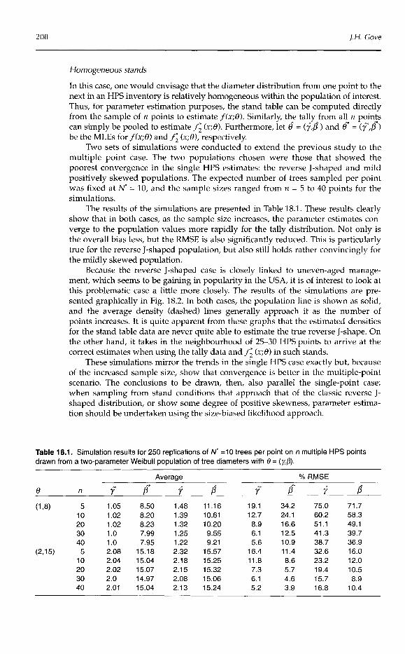
Two sets of simulations were conducted to extend the previous study to the multiple point case. The two populations chosen were those that showed the poorest convergence in the single HPS estimates: the reverse J-shaped and mild positively skewed populations. The expected number of trees sampled per point was fixed at N* = 10, and the sample sizes ranged from n = 5 to 40 points for the simulations.

The results of the simulations are presented in Table 18.1. These results clearly show that in both cases, as the sample size increases, the parameter estimates con- verge to the population values more rapidly for the tally distribution. Not only is the overall bias less, but the RMSE is also significantly reduced. This is particularly true for the reverse J-shaped population, but also still holds rather convincingly for the mildly skewed population.

Because the reverse J-shaped case is closely linked to uneven-aged manage- ment, which seems to be gaining in popularity in the USA, it is of interest to look at this problematic case a little more closely. The results of the simulations are pre- sented graphically in Fig. 18.2. In both cases, the population line is shown as solid, and the average density (dashed) lines generally approach it as the number of points increases. It is quite apparent from these graphs that the estimated densities for the stand table data are never quite able to estimate the true reverse J-shape. On the other hand, it takes in the neighbourhood of 25-30 HPS points to arrive at the correct estimates when using the tally data and f; (x;8) in such stands.

These simulations mirror the trends in the single HPS case exactly but, because of the increased sample size, show that convergence is better in the multiple-point scenario. The conclusions to be drawn, then, also parallel the single-point case: when sampling from stand conditions that approach that of the classic reverse J- shaped distribution, or show some degree of positive skewness, parameter estima- tion should be undertaken using the size-biased likelihood approach.

Table 18.1. Simulation results for 250 replications of N* =10 trees per point on n multiple HPS points drawn from a two-parameter Weibull population of tree diameters with 8 = (y,P).

- -

Average '10 RMSE

Size-biased Distributions in Forestry 2 09

I I I I I

Tallv 0.12

DBH (cm)

Fig. 18.2. Simulated average distribution results for the homogeneous reverse I-shaped population with the tally densities (top) and stand table densities (bottom); the mean densities (dashed) converge to the population curve (solid) with increasing sample size (see Table 18.1 for details).

- 0.04

-0.02

- 0.0

- > + .- - a a n 2

-

a -

Heterogeneous stands

- -

-

-

-

0.02 - - 0.0 -- -

I I I 1 I

/----- Stand

Consider a stand (or larger area) where the diameter distribution varies, possibly considerably, throughout, but where it is still desired to estimate f(x;8). In such cases it may or may not be feasible to stratify.

Stating that the diameter distribution varies is another way of saying that 8 is not constant throughout. For example, consider an HPS with n points in which 8 varies from point to point according to some stochastic process. Thus 8 may be con- sidered a random variable and may exhibit a spatial covariance structure between points. Such a scenario might possibly be modelled using continuous mixtures.

For illustration, assume that the conditional distribution of tallied diameters given 0 is a two-parameter Weibull; Xi I 8 - f ; ( x 1 8). It would then make sense to use a bivariate distribution to model the variation in 0 over the stand. One candi- date probability model for the joint distribution of O - f (8;p,X) is bivariate normal with mean and covariance matrix p and X, respectively. Other bivariate distribu- tions could also be considered. With the bivariate normal, particular care must be taken to ensure that, for all practical purposes, 8 > 0. Thus, extreme variability between HPS points coupled with small-scale or shape parameters might argue against its use. However, for the sake of illustration it is a useful model.

With this modelling scheme, the bivariate normal is the mixing distribution, and the marginal stand tally distribution for Xi under HPS would be given by

210 J.H. Gove

Undoubtedly, the marginal distribution given in Equation 6 does not exist in closed form and the integration would require numerical methods. However, it does pose an interesting interpretation for the final density once yand P have been inte- grated out. The only two remaining parameters are p and Z. Thus, the following method might be used to fit such a distribution based on the techniques discussed earlier in this chapter.

1. Fit a size-biased two-parameter Weibull PDF to each of individual HPS points in the stand using the methods in previous sections. 2. Calculate the sample mean vector and respective sample covariance matrix S from the parameter estimates on the n individual HPS sample points, as estimates of and p and 2, respectively.

The mixture density f ;(x;p,2) may now be estimated by f ;(x;k,S). However, it must be kept in mind that the above has in no way proved that and S have any of the desirable properties of say, MLEs, for p and X. It is simply a possible model for a heterogeneous stand parameter estimation scenario.

Discussion

The discussion on estimation and applications of size-biased distributions to this point demonstrates that they both have a solid theoretical underpinning and practi- cal use in forestry. Well-known relationships between basal area and horizontal point sampling, for example, are preserved under this theory, It should not be sur- prising then that other results will also hold for size-biased distributions. For exam- ple, Gove (2003b) has shown that the relationship between the quadratic mean stand diameter and the harmonic mean basal area from an HPS holds for area-biased dis- tributions; the result is shown to apply also to the BASD.

In fact, size-biased distributions can also bring new insight to previously unknown relationships. For example, Gove and Patil (1998) showed that the third raw moment of the DBH-frequency distribution has an intuitive and consistent inter- pretation through the BASD - a result that had been missed prior to the application of this theory. Similarly, it can be shown analytically (Gove, 2003b) that f(x;O) and f; (x;O) will always cross at the quadratic mean stand diameter (Dq). To illustrate, refer back to Fig. 18.1, for this stand Dq = 28.08 cm, and this is exactly where the two PDFs cross.

A new computer program (BALANCE) (Gove, 200313 has been developed to facili- tate the use of size-biased distributions in forestry. BALANCE was written in FOR- TRAN-90, and is fully integrated with a graphical user interface and runs under Microsoft Windows@ operating systems. Currently, BALANCE allows the user to fit two- and three-parameter equal probability Weibull distributions. In addition, both length- and area-biased versions of these PDFs can also be fitted. BALANCE computes the moment estimates and then uses these as starting values for ML. Results are pre- sented in three windows; a listing of the input data in a grid window, a summary report window with fit statistics, and a graphics window with various graphical dis- plays. The latter may be exported in encapsulated Postscript format, an example of which is shown in Fig. 18.1. Notice in this figure that, even though the equal proba- bility density was estimated for the DBH-frequency distribution, BALANCE also shows the related BASD.

Size-biased Distributions in Forestry 21 1

Clearly, size-biased distributions provide a useful paradigm for sampling and modelling in forestry research. The availability of computer programs such as BALANCE

to make fitting such distributions easier should serve to increase their application.

References

Avery, T.E. and Burkhart, H.E. (1994) Forest Measurements, 4th edn. McGraw-Hill, New York. Bailey, R.L. and Dell, T.R. (1973) Quantifying diameter distributions with the Weibull function.

Forest Science 19,97-104. Cohen, A.C. (1965) Maximum likelihood estimation in the Weibull distribution based on com-

plete and on censored samples. Technometrics 7,579-588. Dennis, B. and Patil, G. (1984) The gamma distribution and weighted multimodal gamma dis-

tributions as models of population abundance. Mathematical Biosciences 68,187-212. Fisher, R.A. (1934) The effects of methods of ascertainment upon the estimation of frequencies.

Annals of Eugenics 6/13-25. Gove, J.H. (2000) Some observations on fitting assumed diameter distributions to horizontal

point sampling data. Canadian Journal of Forest Research 30,521-533. Gove, J.H. (2003a) Moment and maximum likelihood estimators for Weibull distributions

under length- and area-biased sampling. Ecological and Environmental Statistics (in press). Gove, J.H. (2003b) A note on the relationship between the quadratic mean stand diameter and

harmonic mean basal area under size-biased distribution theory. Canadian Journal of Forest Research (in press).

Gove, J.H. (2003~) Balance: a System for Fitting Diameter Distribution Models. General Technical Report. NE-xx, USDA Forest Service (in press).

Gove, J.H. and Patil, G.P. (1998) Modeling the basal area-size distribution of forest stands: a compatible approach. Forest Science 44(2), 285-297.

Gove, J.H., Ringvall, A., StAhl, G. and Ducey, M.J. (1999) Point relascope sampling of downed coarse woody debris. Canadian Journal of Forest Research 29,1718-1726.

Grosenbaugh, L.R. (1958) Point Sampling and Line Sampling: Probability Theory, Geometric Implications, Synthesis. Occasional Paper 160, USDA Forest Service, Southern Forest Experiment Station.

Hyink, D.M. and Moser, J.W. Jr ( 1983) A generalized framework for projecting forest yield and stand structure using diameter distributions. Forest Science 29,85-95.

Kaiser, L. ( 1983) Unbiased estimation in line-intercept sampling. Biometrics 39,965-976. Lappi, J. and Bailey, R.L. (1987) Estimation of diameter increment function or other tree rela-

tions using angle-count samples. Forest Science 33, 725-739. Magnussen, S., Eggermont, P. and LaRiccia, V.N. (1999) Recovering tree heights from airborne

laser scanner data. Forest Science 45(3), 407-422. Mahfoud, M. and Patil, G.P. (1982) On weighted distributions. In: Kallianpur, G., Krishnaiah, P.

and Ghosh, J. (eds) Statistics and Probability: Essays in Honor of C.R. Rao. North-Holland, New York, pp. 479-492.

Patil, G.P. (1981) Studies in statistical ecology involving weighted distributions. In: Ghosh, J.K. and Roy, J. (eds) Applications and New Directions, Proceedings of the Indian Statistical Institute Golden Jubilee. Statistical Publishing Society, Calcutta, pp. 478-503.

Patil, G.P. and Ord, J.K. (1976) On size-biased sampling and related form-invariant weighted distributions. Sankhya, Series B 38(1), 48-61.

Rao, C.R. (1965) On discrete distributions arising out of methods of ascertainment. In: Patil, G.P. (ed.) Classical and Contagious Discrete Distributions. Statistical Publishing Society, Calcutta, pp. 320-332.

Stshl, G. (1998) Transect relascope sampling: a method for the quantification of coarse woody debris. Forest Science 44(1), 58-63.

Taillie, C., Patil, G.P. and Hennemuth, R. (1995) Modeling and analysis of recruitment distribu- tions. Ecological and Environmental Statistics 2(4), 315-329.

Van Deusen, P.C. (1986) Fitting assumed distributions to horizontal point sample diameters. Forest Science 32, 146-148.

212 1.H. Gove

Warren, W. (1975) Statistical distributions in forestry and forest products research. In: Patil, G.P., Kotz, S. and Ord, J.K. (eds) Statistical Distributions in Scientific Work, Vol. 2. D. Reidel, Dordrecht, The Netherlands, pp. 369-384.