
Estimating Water Demand Elasticity at the Intensive and...
49
DEPARTMENT OF ECONOMICS WORKING PAPER SERIES Estimating Water Demand Elasticity at the Intensive and Extensive Margin Daniel A. Brent Louisiana State University (Revised April 2018) Working Paper 2016-06 http://faculty.bus.lsu.edu/papers/pap16_06.pdf Department of Economics Louisiana State University Baton Rouge, LA 70803-6306 http://www.bus.lsu.edu/economics/
Transcript of Estimating Water Demand Elasticity at the Intensive and...

DEPARTMENT OF ECONOMICS WORKING PAPER SERIES
Estimating Water Demand Elasticity at the Intensive
and Extensive Margin
Daniel A. Brent
Louisiana State University
(Revised April 2018)
Working Paper 2016-06
http://faculty.bus.lsu.edu/papers/pap16_06.pdf
Department of Economics
Louisiana State University
Baton Rouge, LA 70803-6306
http://www.bus.lsu.edu/economics/

Estimating Water Demand Elasticity at the Intensiveand Extensive Margin
Working Paper
Daniel A. Brent∗
Department of Economics, Louisiana State University
April 2018
Abstract
I generate a unique panel dataset of monthly water metering records and annual land-scape choices from satellite data for more than 170,000 households over 12 years toestimate price elasticity at the intensive and extensive margin. Higher water prices sig-nificantly increase the probability of adopting water conserving landscapes. Householdsthat maintain dry landscapes are significantly less elastic that the general population.The extensive margin due to landscape accounts for 10% of total elasticity in the shortrun and this increases to 20-26% in the long run. As cities transition away from water-intensive landscapes aggregate demand becomes less elastic it will be more difficult tocope with future droughts by reducing water for residential irrigation.
JEL classification: Q21, Q25, Q54, L95Keywords: water demand; extensive margin elasticity; satellite data; landscape conversion;water conservation
∗Contact: Department of Economics, Louisiana State University; [email protected]. The author is gratefulto Kerry Smith, Michael Hanemann, and Sheila Olmstead for advice and suggestions, as well as HendrikWolff, Joe Cook, and seminar participants at the Camp Resources and Arizona State University’s WaterDemand Workshop for helpful comments. Additionally the author is indebted to Doug Frost and AdamMiller from the City of Phoenix for sharing data and providing insights into water demand in Phoenix.Financial support was provided by Arizona State’s Center for Environmental Economics & SustainabilityPolicy.
1

1 IntroductionPublic water utilities, particularly those in arid regions such as the western United States,
face pressure to fulfill demand with diminished and uncertain supplies. Recently California
suffered through one of the worst droughts on record, which prompted California’s governor
to declare a state of emergency in January 2014.1 Internationally, the east coast of Aus-
tralia recently experienced a one thousand year drought, and the west coast is facing a new
paradigm of permanently strained water supplies. Despite the growing severity of water
scarcity there are gaps in the economic analysis of water demand, particularly with respect
to the complementary goods that use water as an input. Demand for municipal water is
primarily derived from complementary goods, such as washing machines, toilets, showers,
and gardens that collectively comprise the capital stock for water. In the residential sector
landscape is the most important complementary good. In the context of water demand,
adjustments to the water capital stock represent changes along the extensive margin, while
the intensive margin constitutes behavioral changes conditional on a fixed set of comple-
mentary goods. The lack of research on the extensive margin elasticity is concerning given
the resources specifically devoted to upgrading complementary goods, as evidenced by the
approximately $450 million spent on removing turf grass by the Metropolitan Water District
of Southern California.
The conventional treatment of the extensive margin in the water demand literature relies
on the assumption that households cannot fully respond to prices in the short run due
to frictions that prevent the immediate replacement of complementary goods. Therefore,
the long run equilibrium, where full adjustment takes place, encompasses changes along
both the intensive and extensive margins. Earlier water demand research employs partial
adjustment models that include lagged consumption in the demand equation, and find that
long run elasticity exceeds short run elasticity in absolute value (Billings and Agthe, 1980;
Carver and Boland, 1980; Dandy et al., 1997; Pint, 1999; Nauges and Thomas, 2003; Bell
and Griffin, 2011). The notion that demand is more elastic in the long run is a standard
result from economic theory, and implies that there are meaningful reductions in water
consumption along the extensive margin by replacing complementary goods such as turf
lawn. The limitation of the flow-adjustment models is that they estimate changes along the
extensive margin implicitly through a parametric specification of demand. While explicit
treatment of the capital stock has been studied in energy markets (Dubin and McFadden,
1984; Vaage, 2000; Goulder et al., 2009; Busse et al., 2013; Gillingham, 2014; Newell and
Siikamaki, 2014; Allcott and Wozny, 2014) there is little research devoted to changes in the
water capital stock.
1See details at http://ca.gov/drought/.
2

This paper’s primary objective is to incorporate changes in landscape choices over time
into a model of water demand, which allows me to make three contributions to the water
demand literature. First, I incorporate landscape decisions in a two-stage model to esti-
mate the effect of price on consumption through the channel of landscape change. Second, I
isolate the intensive margin elasticity by estimating conditional demand functions for house-
holds that maintain a fixed landscape over the course of the sample. Third, I examine the
long-run effect of water rates on water-efficient landscape adoption, as well as the impact of
landscape conversions on water demand. The primary barrier to addressing these objectives
in the previous literature is the need to observe changes in both water consumption and
landscape over time. My approach merges a spatially explicit time series of satellite data
capturing vegetative cover at the parcel level to monthly water metering records and struc-
tural characteristics of the home. The result is a novel panel dataset of nearly 25 million
observations of water and landscape for over 170,000 households in City of Phoenix. This is
complemented with a dataset on landscape, housing characteristics, and water rates for over
370,000 households spanning eight municipalities in the Phoenix metropolitan area.
The primary result is that water rates affect landscape choices; higher prices increase
the probability that households adopt water-efficient landscapes. Landscape choices also
have a significant effect on water consumption. Combining results on the effect of price
on landscape and the impact of landscape on demand generates estimates of the extensive
margin elasticity of demand due to changes in landscape. In the two stage model for annual
landscape choice and water demand, the extensive margin represents roughly 10% of the total
demand elasticity. In the long run model of dry landscape adoption the share of the extensive
margin increases to 20-26% of aggregate elasticity. Across all specification prices increase the
probability of adopting water efficient landscapes. The results are robust to multiple model
specifications and a boundary discontinuity analysis that restricts the sample to households
near utility borders.
There are also lessons for water management policy based on the heterogeneity in water
demand due to landscape. Households that maintain a dry landscape throughout the sample
are significantly less price elastic than the general population. This has implications for how
the aggregate elasticity will change as households in arid regions convert to dry landscapes.
Neighbors’ landscape choices are also positive and significant determinants in the conversion
decision, although I caution a causal interpretation of this results due to the challenge in
identifying peer effects (Manski, 1993, 2000). The empirical association between neighbors’
landscape choices is consistent with anecdotal evidence of the importance of social peer ef-
fects that lead to the transition towards drought-resistant landscapes as social norms evolve.
Landscape conversions have a large impact on demand; converting landscape from wet to
3
dry decreases water consumption by roughly 20%. The results demonstrate that the price
mechanism, as opposed to commonly employed mandatory watering restrictions, can effec-
tively curtail outdoor water use; an outcome that economists have shown improves social
welfare (Grafton and Ward, 2008; Mansur and Olmstead, 2012).2
While there are many complementary goods that comprise the extensive margin in water
demand, I focus on landscape due its three important characteristics. First, irrigation for
landscapes consumes massive quantities of water. In cities with an arid climate, such as
the southwestern United States, outdoor water use represents 50% or more of aggregate
demand, of which up to 90% is for landscape (Dandy et al., 1997; Wentz and Gober, 2007;
Balling et al., 2008). Second, residential irrigation is a discretionary use as opposed to water
for drinking and sanitation.3 Lastly, demand for landscape irrigation is countercyclical to
supply with demand rising during droughts and heat waves when water supplies are stressed.
Understanding the interaction between landscape and water demand has important im-
plications for water management during droughts. There are multiple studies that measure
the efficacy of demand side management policies that come into effect during water shortages
(Nataraj and Hanemann, 2011; Klaiber et al., 2014; Ferraro and Price, 2013; Brent et al.,
2015; Wichman et al., 2016). One of the most common command and control policies is
limiting outdoor water use for lawns and gardens during times of drought. Estimates of the
welfare loss from using mandatory restrictions as opposed to prices range from $96 to $152
per household per season (Grafton and Ward, 2008; Mansur and Olmstead, 2012).4 Water
managers face the challenge of quickly reducing demand under the constraint that water
consumption is a function of the quasi-fixed complementary goods. Given the importance
of managing outdoor water use during droughts, and the welfare loss associated with tradi-
tional policies, it is critical to assess the ability of the price mechanism to curtail outdoor
water use through landscape conversions. Despite the importance of demand for residential
irrigation during drought conditions, there is no research that directly incorporates changes
in landscape into water demand by modeling the landscape conversion decision.5 The de-
cision to maintain a lush green landscape, or switch to drought-resistant vegetation, alters
the behavioral response to water rates and weather conditions leading to structural changes
2One advantage of using mandatory restrictions instead of prices during droughts is that restrictionsproduce an immediate decrease in consumption, while consumers may take time to adjust to prices.
3This limits concerns about pricing water that is considered a human rights. The United Nations,through Resolution 64-292, deemed clean drinking water and sanitation to be a human right, while waterfor discretionary uses is widely considered to be an economic good (Perry et al., 1997).
4The alternative to mandatory restrictions is supply disruptions, which Buck et al. (2016) also show havelarge welfare consequences.
5Tchigriaeva et al. (2014) does address heterogeneity due to landscape, but does not incorporate changinglandscape over time and Brelsford and Abbott (2018) examines response to turf rebates.
4

in demand.
Landscape conversions have long run implications for water demand since water-intensive
landscapes act as an additional source of supply that can be drawn down during times of
drought through reductions in irrigation. The empirical results indicate that demand pa-
rameters such as the responsiveness to price and weather variables evolve as the composition
of residential landscapes changes. As consumers transition to water-efficient landscapes
aggregate demand becomes less elastic, and there will be less capacity to rapidly reduce con-
sumption during droughts. Since climate change is anticipated to increase the probability
of severe sustained droughts, it is critical to measure the distribution of green landscapes
and understand the heterogeneity of consumer response to policy interventions. Utilizing
satellite data adds depth to water demand estimation and informs policy makers about the
long run effects of rate increases, and how consumers will respond to future price changes.
2 Background & Data
2.1 Water and landscape in PhoenixPhoenix lies in an arid climate and its history is inextricably tied to importing water from
external sources. The prodigious water infrastructure projects conducted by the U.S. Bureau
of Reclamation in the early 20th century enabled the development of a strong agricultural
sector by securing water rights from the Colorado River via the Central Arizona Project,
with additional water sourced from the Verde and Salt Rivers via the Salt River Project.
The experience of engineering solutions for water scarcity by transporting and storing vast
volumes of water has been replicated in many Western regions, and facilitated rapid popu-
lation growth in the southwestern United States.6 During Phoenix’s transition into a major
metropolis in the second half of the 20th century, the water rights freed up from converted
agricultural land allowed residential developments to establish lush green landscapes with
immense water requirements. As water rates rise and environmental issues related to water
scarcity become more prominent, households are now converting their green landscapes to
drought-resistant native vegetation, known as xeriscape or xeric landscape.
Supply constraints are stressed during the summer peak demand period, and for this
reason I focus on summer demand, defined as June through September. Additionally, the
link between landscape and water demand is strongest during the summer.7 Landscape
conversions normally take place from October-May in order to avoid the extreme heat of
the summer months, making observations of the landscape at any point between May and
6According to data from the 2010 census, Phoenix was the sixth largest city in the U.S., with nearly 1.5million inhabitants and a metro area that includes 6 other municipalities with over 200,000 people.
7There is also evidence summer water demand is inherently different and lumping winter and summerdemand together is not appropriate (Dalhuisen et al., 2003; Espey et al., 1997; Bell and Griffin, 2011).
5

September good indicators of the landscape during the summer season. Summer landscape
has a high fixed costs of conversion, so a landscape conversion is typically a long-run decision.8
Conversely, Bermuda turf, the most common grass in the Phoenix area, lies dormant in the
winter and consumers need to reseed each season in order to have a green lawn in the winter.
Therefore some households’ green summer lawns will appear dry in the winter even if they
still have turf grass. Households may also refrain from watering their lawns in the summer,
which will have the same satellite signature as a xeric landscape.
A key feature of water demand in the Phoenix metropolitan area is the Salt River Project
(SRP). The SRP provides irrigation water to households within its service area through
a system of canals. Water is delivered to households approximately every two weeks in
the summer via flood irrigation, where the lawn is flooded with several inches of water.
Residential customers pay an annual fee of roughly $60 for this service that covers a base
quantity of water, which is sufficient for most households’ landscape irrigation. Not all
households within the SRP service area sign up for this service since the flood irrigation
requires a depressed lawn in order to hold the water and is known to attract pests. Households
within the SRP water still use municipal water for indoor use, filling pools, and supplemental
landscape irrigation. Since the SRP affects water use on both the intensive and extensive I
incorporate this source of heterogeneity in the analysis. See Figure 1 for the geographical
boundaries of the SRP.
2.2 DataData limitations constrain existing empirical studies of water demand. In order to in-
corporate capital goods into water demand I utilize a time series of satellite data obtained
from the National Aeronautics and Space Administration’s (NASA) Landsat 5 Thematic
Mapper series, henceforth referred to as Landsat.9 The Normalized Difference Vegetation
Index (NDVI), one of the most common measures of vegetative cover, serves as a proxy
for landscape choices (Aggarwal et al., 2012; Stefanov and Netzband, 2005; Stefanov et al.,
2001).
Since Phoenix is an arid environment with few cloudy days I can acquire high-quality
images during the summer for each year. For each summer period I use two images to capture
the average landscaping patterns, and to limit the impact of random weather events.10 Each
image represents an observation at one point in time and there are several steps to process
the data to ensure comparability over time and space, described in detail in Section A.1
8Average yard size is approximately 7000 square feet (lot size less square footage of house). If half ofthat the yard is turf and conversion costs range between $1.5-$2.5 per square foot, then conversion costsrange from $5,250-$8,750; from http://www.mesaaz.gov/conservation/convert.aspx.
9Landsat data, publicly available for download from the USGS Glovis system at http://glovis.usgs.gov/.10There were two valid images in the summer for every year except 1998, where only one image was used.
6
of the Appendix. The final landscape dataset is a panel where the cross-sectional unit is
geographical location and the time series is the year. Although there is a continuum of
landscaping options in the Metro area the two overarching categories are drought-resistant
native plants, (xeric), and lush green vegetation usually comprised of turf lawn and referred
to as mesic.
The key distinction for this research is that xeric landscapes are much less water-intensive
than mesic landscapes. Exact classification is not the primary concern; rather I develop a
variable that captures the general water requirements for landscaping at the parcel level.
Since NDVI captures the intensity of vegetation for a given area, and water is required to
maintain almost all vibrant green vegetation in Phoenix, the index is appropriate for this
coarse classification. For the rest of the paper, xeric and dry will be used interchangeably
to define low-NDVI landscapes as will mesic, green, and wet for high-NDVI landscapes. In
order to obtain accurate landscape classifications I compare quantiles of NDVI, which ranges
from -1 to 1, with the data from a widely-cited existing remote sensing study Stefanov et al.
(2001).11 NDVI performs well in classifying landscape at the tails of the distribution, and is
less accurate in the middle of the distributions. Table A.2 displays the comparison of NDVI
quantiles with the classification of Stefanov et al. (2001).
A limitation of validating the use of NDVI for landscape classification in this study is
that data in Stefanov et al. (2001) are only available for one year, and the purpose of this
research is to observe both water and landscape over time. Comparing quantiles of NDVI
over time is problematic because NDVI is correlated with time-varying weather conditions.
In order to improve comparability of NDVI across years I regress NDVI on weather vari-
ables to parse out the variation due to weather. Section A.3 of the Appendix describes the
normalization procedure and presents results from the weather normalization regressions.
Using the residuals from the weather normalization regressions I create quantiles over the
distribution of normalized NDVI. Weather data are collected from three sources: the Na-
tional Oceanic and Atmospheric Administration’s National Climatic Data Center, Oregon
State University’s PRISM Climate Group, and the University of Arizona’s AZMET Weather
Data.12
In addition to the landscape and weather data I obtain geo-referenced parcel character-
istics from the Maricopa County Assessor, socioeconomic data and census boundaries from
the U.S. Census, and water metering records from the City of Phoenix. These data sources
produce two final datasets: a monthly panel of water metering records for 172,314 house-
11As of 4/6/2018 Stefanov et al. (2001) had 501 citations in Google Scholar.12The data are all publicly available at the following websites: http://www.ncdc.noaa.gov/ (NOAA),
http://www.prism.oregonstate.edu/ (PRISM), http://ag.arizona.edu/azmet/azdata.htm/ (AZMET).
7
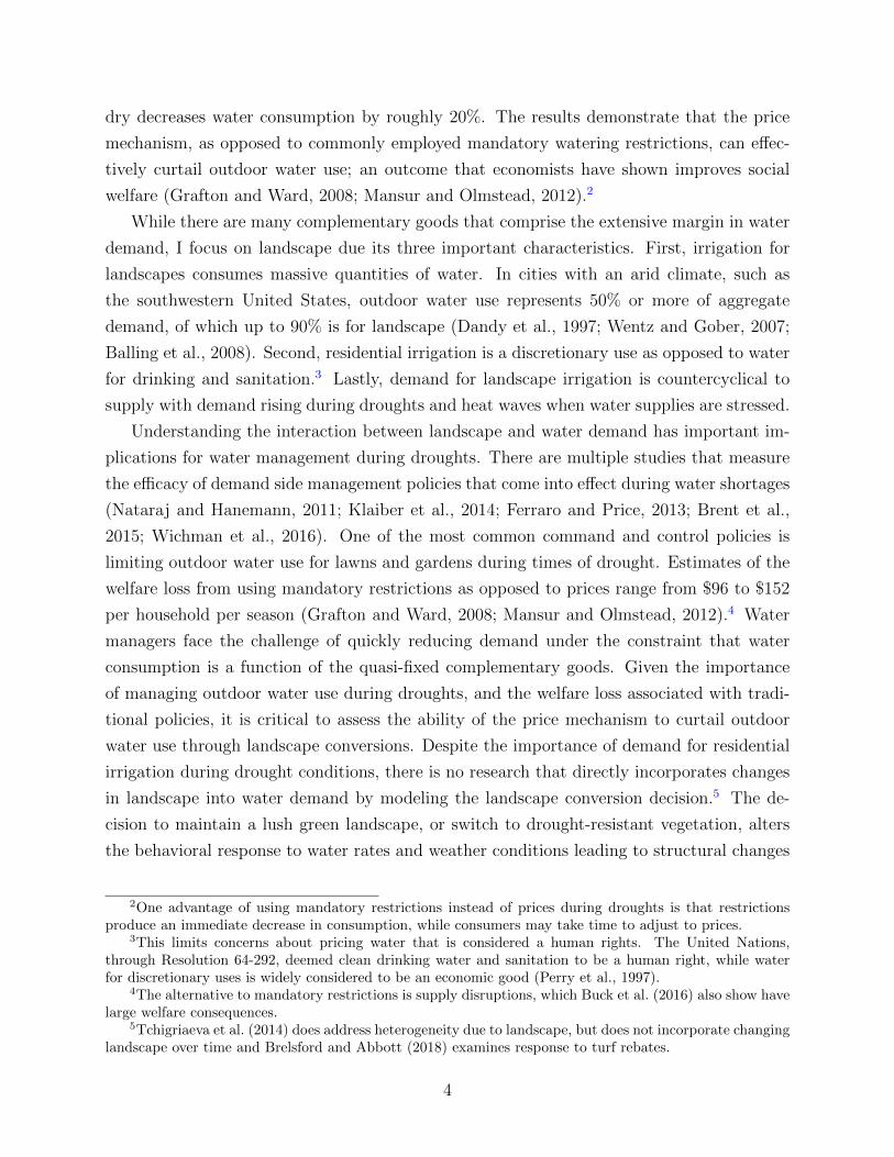
holds in the City of Phoenix and a yearly panel of landscape choices for 370,781 households
in the Phoenix metropolitan area that span eight distinct municipal water providers. Figure
1 shows a map of the sample area including the parcels, metropolitan areas (with Phoenix
outlined in bold red), and the border of the Salt River Project. The City of Phoenix data
will be referred to as the Phoenix (or PHX) data and the metropolitan area data will be
referred to as the Metro data. The primary purpose of the Metro data is to introduce spatial
variation in the long run changes to water rates when estimating the effect of prices on long
run dry landscape adoption.
Figure 1: Phoenix Metro Area
Note: The map shows the the parcels used in the analysis along with the municipality geographies and theSRP boundary.
2.2.1 City of Phoenix Water Dataset
Water consumption data are only available within the City of Phoenix, and therefore all
water demand models are estimated exclusively within Phoenix data. Water consumption
is observed though monthly metering records for single-family homes in the City of Phoenix
Water Department’s service area from 1998-2009. This rich dataset is a balanced panel
containing nearly 25 million observations, with over 8 million observations during the summer
demand period. Since this period corresponds with the collapse of the housing market,
using data from active accounts ensures that dry landscapes in the Phoenix data are not
merely neglected lawns of foreclosed homes. I spatially merge NDVI, structural housing
characteristics, selected census demographic variables, and weather variables for each single
8

family residential parcel in Phoenix to the time series of water metering records and water
rates.13 The resulting dataset is a panel with two sources of time-varying data. Water
consumption, water rates, and weather all vary at the monthly level, whereas NDVI varies
annually. Structural characteristics of the house are recorded at the time of the sale and
thus can vary over time, but the vast majority of the structural features of the house remain
constant during the sample.14
In the Phoenix data I form three groups based on the time series of satellite data: Wet,
Dry, and Mixed. The Wet and Dry groups contain households that, for every year in the
sample, have a normalized NDVI value above the 70th percentile or below the 30th percentile
respectively.15 The Mixed group makes up the remainder of the sample and consists of
households that converted from wet to dry landscapes, converted from dry to wet, or have at
least one normalized NDVI observation that lies between the 30th and 70th percentiles. It
is possible that the Mixed group has a combination of turf grass and native vegetation, but
I cannot distinguish different landscape patterns within a parcel with the Landsat remote
sensing data. To clarify the notation, wet/dry are general descriptors for annual landscape
classifications, whereas the capitalized versions Wet/Dry correspond to the formal groups in
the sample that are consistently wet or dry.
Examining summary statistics for each of the three landscape groups in Table 1a reveals
that the landscape groups differ by several variables that impact water consumption, and may
affect demand elasticity. Unsurprisingly, the Wet group on average uses roughly one third
more water than the Mixed group and two thirds as much as the Dry group. Additionally,
the Wet group lives in larger, older, and more expensive homes. Therefore, there may be
unobservables driving differences in water demand as well, and for these reasons I run models
that control for selection into each landscape group.
In addition to the classification diagnostics with respect to the Stefanov et al. (2001)
study, merging the landscape data with water consumption records confirms that the satel-
lite data performs well as a proxy for landscape. Figure 2 shows the average historical
consumption for the three groups. While all groups have a cyclical dimension to consump-
tion, seasonality is much stronger for the Wet group, and in fact these households are the
13According to a confidentiality agreement with the City of Phoenix I merge the NDVI values at theparcel level and then City officials attached it to an anonymous identifier representing a water account.
14I can only observe changes in structural housing characteristics for homes that are sold multiple times inthe sample, which comprise 43% of the sample. Within this subset of homes most structural characteristicsdo not change. For example only 0.8% of households in the sample are observed either adding or removinga pool.
15The results from the classification diagnostics in the Appendix reveal that performance of NDVI for dryextends out from the tails to a greater degree than for wet. I also consider using non-symmetrical cutoffs forlandscape classification in order to obtain a relatively balanced group for Wet and Dry. This is explored inthe robustness and the results are robust to changing the NDVI classification thresholds.
9

primary driver of peak summer demand. In the winter months all three groups converge
while there are extreme differences in summer usage. To put these consumption figures in
perspective according to the U.S. Environmental Protection Agency average household con-
sumption is approximately 300 gallons per day.16 So while the Dry group still uses more
water in the summer relative to the U.S. average, the Wet group’s summer usage is more
than twice the average U.S. household.
Figure 2: Water Consumption by Landscape Group
Note: Wet and Dry groups are determined by those that were continuously above the 70th percentile and below the 30thpercentile of NDVI respectively. The Mix group is the remainder of the sample.
2.2.2 Landscape Conversion DatasetIn order to augment the Phoenix dataset and introduce cross-sectional variation in water
rates, I incorporate data from the surrounding municipalities in the Phoenix metropolitan
area (Metro) when modeling long run dry landscape adoption, which constitutes the central
component of the extensive margin. I spatially merge the time series of NDVI, structural
housing characteristics, selected census demographic variables, and weather variables to each
single family residential parcel in the Metro area. In order to avoid the foreclosure problem
for the Metro data, for which there are no water consumption records, I focus on the period
1998-2006 prior to the financial crisis that hit Phoenix particularly hard (see Figure A.1). I
also drop all houses that were built after 1998 to maintain consistency with the CoP water
data. Lastly, I merge in historical water rates data for each of the eight municipalities as
well as policies related to rebates for turf conversion. The resulting dataset is a panel with
the parcel as the cross sectional unit and a year as the time series.
16Estimates from the U.S. Environmental Protection Agency are available athttp://www.epa.gov/watersense/our water/water use today.html.
10

Similar to the Phoenix each of the water utilities employs some form of increasing block
pricing. My primary specification of water rates is to use the highest marginal price in
the rate structure. This avoids the need to observe consumption to determine the price.
The maximum marginal price is also appropriate for determining the impact on landscape
because most increasing block rates use the highest tier to target outdoor water use such as
irrigation. Therefore, the maximum marginal price is a relevant metric for the cost of water
in the landscape conversion decision. As a robustness check I also estimate the marginal and
average price for each household outside of Phoenix using an out of sample prediction for
each household’s water consumption from a regression of water on housing characteristics,
weather, and time fixed effects using the Phoenix sample. This assumes that the relationship
between house size, pool ownership, and other characteristics is similar for Phoenix and the
other municipalities. Using the estimated consumption and each municipality’s rate structure
I calculate the average and marginal price for each household. Table 1b shows the summary
statistics for relevant variables by municipality.
Table 1: Summary Statistics
(a) Water Dataset - City of Phoenix
Landscape Group Water Use Lot House Price Year Built Pool HouseholdsMix 21.7 8,686 121,845 1972 0.34 132,673Dry 17.3 8,119 122,742 1977 0.33 14,028Wet 28.9 11,254 172,386 1965 0.39 25,614
(b) Landscape Dataset - Metro Area
City Convert Rate AP MP MxP Rebate Lot House Price Year Built HouseholdsChandler 1.2 1.38 1.01 1.39 200 7,721 141,578 1986 31,610Gilber 0.6 1.28 0.69 0.93 0 9,559 169,996 1992 23,069Glendale 2.6 0.92 1.08 1.39 375 9,005 135,303 1981 36,960Mesa 1.9 0.65 1.78 1.81 0 8,255 138,530 1985 9,739Peoria 2.1 1.41 2.1 2.51 1,650 8,501 138,461 1989 21,573Phoenix 3.1 1.09 1.8 1.8 0 9,276 135,912 1971 194,193Scottsdale 1.2 0.73 1.71 1.78 625 14,114 280,250 1981 37,812Surprise 0.3 1.99 1.61 1.61 0 8,056 160,489 1994 4,180Tempe 2.6 0.84 0.71 0.87 150 8,312 125,658 1967 11,645All 2.4 1.08 1.56 1.68 218 9,512 153,346 1977 370,781
Note: In panel (a) water use is in ccf/month, Lot is square feet, House price is in dollars, Pool is the fraction of households witha pool. In panel (b) Convert Rate is the percentage of households that converted in that city, AP is average price per ccf, MPis marginal price per ccf, MxP is the maximum price per ccf, and Rebate is the average maximum rebate for turf conversion indollars. Variables present in both panels have the same units.
The water rates for the various municipalities are shown in Figure 3. Panel (a) shows
the maximum marginal price and Panel (b) shows the average price. For all municipalities
other than Phoenix the average price is calculated using predicted water consumption as
described above. Most utilities have experienced increases in the water rates, although the
rate of increase over the sample is quite different across utilities. All prices are in 2008
11

dollars.
Figure 3: Water Rates
(a) Maximum Marginal Price (b) Predicted Average Price
Note: Panel (a) shows the maximum marginal price in dollars per CCF for each year in each utility. Panel (b) shows thepredicted average price in dollars per CCF for each year in each utility. Since each consumer may have a different average pricethe graph shows the average price averaged over all consumers. All prices are in 2008 dollars.
3 Estimation StrategyObserving changes in the capital stock and water use over time add richness to modeling
water demand, and allows for demand estimation on the intensive and extensive margin.
The framework can be applied to other goods such as washing machines or toilets given data
availability. In this context I define the intensive margin as changes in water consumption
holding landscape constant; changes in the capital stock for other goods are incorporated
into the intensive margin. For these reasons, elasticity estimates for the intensive margin
should be considered upper bounds, while the extensive margin estimates are effective lower
bounds.
To simplify the notation assume there are only two types of landscape: wet and dry
(ignoring the mixed group for now).17 Similar to Dubin and McFadden (1984) I disaggregate
water demand elasticity into probability weighted averages conditional on landscape. In this
setting average water consumption is represented as Erws “ PdryErw|drys ` PwetErw|wets,
where Erw|drys and Erw|wets are the conditional expectations of water consumption given
a dry and wet landscape; and Pdry, Pwet are the fractions of households with dry and wet
17Note that these are not the same definitions as Wet and Dry, rather these are colloquial terms thatdesignate two general landscaping regimes.
12

landscapes. The general notation for the elasticity of x with respect to y is εpx, yq and pw is
the price of water.
εpErws, pwq “ εpErw|drys, pwqPdry
ˆ
Erw|drys
Erws
˙
` εpErw|wets, pwqPwet
ˆ
Erw|wets
Erws
˙
` εpPdry, pwqPwet
ˆ
Erw|drys ´ Erw|wetsq
Erws
˙
(1)
The first two terms of equation 1 are the probability weighted averages of the conditional
elasticities for dry and wet households respectively, and the last term captures the impact
of price on dry landscape adoption. There are two key insights in equation 1. First, hetero-
geneity exists in the intensive margin elasticity based on the type of landscape, displayed as
εpErw|drys, pwq and εpErw|wets, pwq. Second, the extensive margin elasticity measures the
impact of price on the proportion of households with dry landscapes, εpPdry, pwq, scaled by the
change in consumption from converting from a wet to a dry landscape, PwetErw|drys´Erw|wets
Erws.
Estimating the separate elements of equation 1 requires a time series of landscape decisions
to identify changes in landscape as well as households that preserve a fixed landscape. I
estimate the model using two different methods described in detail below: 1) a two stage
model of annual landscape choice and monthly water demand and 2) separate models for
conditional demand and long run dry landscape adoption.
3.1 Short-Run Two Stage ModelThe first approach to incorporating landscape into water demand is a two stage model.
The first stage models the impact of price and other factors on landscape choice and the
second stage estimates a water demand model augmented by the predicted probabilities for
each type of landscape from the first stage. The first stage landscape choice model is defined
as:
Lit “ γl1pit´12 ` βX1it ` ξit (2)
where Lit P tmixed, dry, wetu represents the three landscape choices, and pit´12 are the water
prices from the previous year (12 months). The coefficient on price, γl1, captures the effect of
price on the probability for selecting a dry or wet landscape relative to the mixed class. I also
include other variables in X 1it to predict landscape choice such as structural features of the
house, neighborhood demographic variables, the number of neighbors with dry landscapes,
and a dummy indicating if the house was sold in the year leading up to the summer demand
period. The error term, ξit, is assumed to follow the type-I extreme value distribution leading
to a multinomial logit model. From the landscape choice model I calculate the predicted
probabilities for having a dry or wet landscape in a given year and use these in the second
13
stage water demand model defined as:
lnpwitq “ αi ` γl2lnppit´1q ` δdryPdry ` δwetPwet ` βX
1it ` εit (3)
where lnpwitq is the natural log of monthly household water consumption, lnppit´1q is the
logged water price from the previous month. The predicted probabilities for dry and wet
landscapes from the first stage landscape model are Pdry and Pwet, with mixed being the
omitted class. Additional control variables in X 1it include weather variables and a time
trend. The water demand model includes household fixed effects (αi) and εit is a normally
distributed idiosyncratic error term. To account for the two-stage process the standard
errors in the water demand model are bootstrapped across both stages, re-sampling at the
household level. In the two stage model the extensive margin is the effect of price on
landscape in the first stage multiplied by the effect of landscape on water demand in the
second stage. The elasticity parameter in the second stage accounts for the effect of price
on water demand through all channels other than landscape.
3.2 Long-Run Landscape Adoption ModelThe two stage model is appealing because it simply incorporates landscape choices into
water demand, however, households are allowed to choose a different landscape each year.
In reality changing landscape from turf lawn to xeriscape is a costly long-term investment.
Therefore, another way to model landscape choice is to focus on dry landscape adoption
in the long run. The long run model consists of three parts. First, I estimate conditional
demand functions based on the time series of landscape choices for three types of households:
consistently dry (Dry), consistent wet (Wet), and neither consistently wet nor dry (Mixed).
Second, I estimate the long run effect of changes in prices on the probability of having a
dry landscape. Lastly, I estimate how landscape conversions affect water consumption. It
is important to note that the conditional demand regressions and the effect of landscape
conversions on water demand (parts one and three) are conducted with the Phoenix data,
whereas the impact of price on dry landscape adoption (part two) uses the Metro data.
The conditional demand functions are defined as
lnpwlitq “ αli ` γllnppit´1q ` β
lX 1it ` ε
lit (4)
where wit is water consumption for household i at time t, pit is the price of water, Xit is
a vector of weather controls, αi is a household level fixed effect, and ξit is an idiosyncratic
error term. The superscripts refer to the landscape groups, where l “ tMixed,Dry,Wetu.
The dependent variable is the log of monthly water consumption, and the parameters of
interest are the values of γl for each landscape group, interpreted as elasticities in the log-log
specification.
As seen in Table 1 there are significant differences in the characteristics of the house-
14

holds across the landscape groups. Therefore, there may be issues of sample selection in
the conditional demand functions since the differences in elasticity estimates may be due
to underlying individual heterogeneity, irrespective of landscape, between the three groups
(Heckman, 1974). The conditional demand functions presented in Table 3 all contain house-
hold fixed effects that capture static unobserved heterogeneity that is idiosyncratic to the
household. However, to address issues of sample selection for the time-varying unobserv-
ables across landscape groups, I use sample selection corrections employed by Dahl (2002)
utilizing third order polynomials of predicted probabilities from the selection equation in the
conditional demand functions. These models require strong functional form assumptions if
there is no exclusions criteria: variables that show up in the selection equation but not if the
conditional demand regressions. The selection equation utilizes two significant time-varying
variables that are plausibly exogenous: neighbors’ conversions and a dummy whether the
house was sold in the previous year.18 As seen in Table A.4 these are key indicators of
landscape conversions and they are plausibly exogenous to water use. Neighbors’ landscape
is a particularly attractive variable to account for selection because it captures time-varying
unobserved heterogeneity at the neighborhood level. All regressions that include selection
correction estimate the standard errors with bootstrap methods that re-sample at the house-
hold level to account for the two-stage estimation.
The decision to replace turf grass with native desert plants is a major investment for a
household. The benefits are a sequence of savings from lower water consumption as well as
reduced labor costs if the xeriscape requires less maintenance, as is often the case. Costs of
conversion consist primarily of the upfront fixed cost of the conversion; for example one set
of estimates from Las Vegas range from $1.37-1.93 per square foot (Sovocool et al., 2006).19
The landscape conversion model treats landscape conversion as an irreversible investment
since it is unlikely that a household will re-install grass after an expensive investment in
xeriscape due to the high fixed costs. This is similar to the decision to invest in residential
energy efficiency (Hassett and Metcalf, 1995; Revelt and Train, 1998), development and land
use (Butsic et al., 2011; Schatzki, 2003), technology adoption (Farzi et al., 1998), and factory
exit decision (Biørn et al., 1998).
I model the timing of landscape conversion as the product of a household optimization
problem such that a household chooses the time of conversion T to minimize:
V “
ż T
0
rptW ` pmt ´ btqse´ρtdt`
ż 8
T
p1´ θqptWe´ρtdt`Kte´ρt (5)
18The results of the selection equation and results are described in more detail in Section A.6 of theAppendix.
19The Sovocool et al. (2006) estimates are from 2001 and match up with those for the Phoenix area afteraccounting for inflation. In 2010 dollars the conversion costs are $1.80-2.54, within the range of $1.50-2.50reported for the Phoenix area.
15

where pt is the price of water at time t, W is the water requirement for a green landscape,
mt is the maintenance cost (outside of water costs) of a green landscape relative to a dry
landscape, and bt is the dollar value of the relative benefits of a mesic landscape compared to
xeric. There is a one-time cost of Kt to convert a landscape, taken to be the numeraire, and
I assume a conversion achieves a proportional reduction in water consumption by a factor
θ. The discount rate is ρ and is less than one. The first order condition to this optimization
problem that dictates whether, and when, a household will convert is
θpT W ` pmT ´ bT q ´ ρKT ě 0 (6)
If the water savings and non-water costs of a green landscape exceed the discounted capital
cost then a household will convert. The term pmt ´ btq captures the non-water component
of the landscape decision with bt representing the visual appeal and recreational value of
a grass lawn, whereas mt consists of labor and material costs associated with landscape
maintenance.
In order to analyze long run changes in prices on landscape choices I estimate equation
7, which is a long-difference model that examines the probability of having a dry landscape
by the end of the sample based on changes in prices, rebates, and neighbors decisions.
This analysis accounts for all households, including those that start the sample with a dry
landscape, and thus includes the effect of price on dry households remaining dry rather than
switching to wet. I parameterize εi in equation 7 as normally distributed leading to a panel
data linear probability model.
Di “ α ` γLRpi ` φri ` xiβ ` εi (7)
This is no longer a panel model since the dependent variable is not time varying, rather Di
is a dummy that is equal to one if a household is dry at the end of the sample. Ending prices
and rebates (pi, ri) are subtracted from initial values. The term xi includes the long run
difference in the fraction of neighbors’ with dry landscapes, the number of times the house
was sold during the sample, and an indicator for whether the household had a wet landscape
at the beginning of the sample. The long run model requires cross sectional variation in the
long run price changes and therefore is only estimated with for the Metro sample.
In order to complete the extensive margin elasticity calculation I estimate the impact
of conversions on water demand. A simplistic approach is to multiply the marginal change
in the conversion probability by the difference in average consumption between the Wet
and Dry group. A problem with this methodology is that the Wet and Dry groups may
have fundamental differences because, by definition, they do not convert during the sample.
In order to estimate the impact of conversions on water demand I create a variable that
designates whether household i experienced a conversion at time t defined by Cit, which is
equal to one if household i converted prior to time t and zero otherwise.
16

Augmenting the water demand model with landscape conversions, Cit, estimates the
impact of conversion on consumption. Incorporating conversions into water demand also
provides a validation test for the conversion classification by linking it back to water me-
tering data. Since the NDVI data is relatively coarse there is a concern that the landscape
conversion model is actually picking up landscape decisions of neighboring parcels instead
of the parcel itself.20 To test for this potential problem I create a variable for how many
neighbors have converted their landscape. ˜NCit is the sum of non-contiguous neighbors’
conversions. The augmented water demand model is defined by:
lnpwitq “ αi ` γlnppit´1q ` βXit ` δ1Cit ` δ2˜NCit ` εit (8)
Since I only observe water consumption for City of Phoenix Equation 8 is estimated with
the City of Phoenix data, and I assume that the savings due to landscape conversions is
similar for the other municipalities in the Metro data.
3.3 Water Price SpecificationBefore estimating the water demand functions I perform model specification based on
the aggregate sample by estimating the water demand function presented in equation 4. The
motivation for the model specification is that the City of Phoenix has an increasing block
rate, leading to several potential specifications for the relevant water price to consumers.
There is an active debate in the economics literature whether consumers facing nonlinear
budget constraints respond to the average or marginal price (Nataraj and Hanemann, 2011;
Baerenklau et al., 2014; Klaiber et al., 2014; Ito, 2014; Wichman, 2014).21 In reality price
response is likely heterogeneous and certain rate structures may generate aggregate demand
that is best modeled as either average or marginal price response (Olmstead et al., 2007).
In Phoenix the price signal primarily stems from the volumetric charge in the second
block, and it is likely that even consumers in the first block respond to the price for the
second block. The first block is set at 10 hundred cubic feet (CCF)22 in the summer and the
price in this block ranges from $0.09-0.39 over the sample; yielding a maximal variable cost
in the first block of less than $4.00 per month. Looking at the data, almost 80% of monthly
observations are in the high block and fewer than 0.6% of households never consume in the
high block. Given the nature of the Phoenix rate structure it is probable that the high
marginal price is more relevant for consumer demand than the actual marginal price. I run
20This is unlikely because the immediate contiguous neighbors are removed when creating variables forneighbors landscapes precisely to address this concern.
21Shin (1985) was one of the first to acknowledge that acquiring price information is costly in the presenceof nonlinear rate structures, and that consumers may rationally choose to use average price instead ofmarginal price if the benefits to using marginal price do not outweigh the costs of learning the actualmarginal price.
22One CCF equals approximately 748 gallons.
17

three specifications of the price in the water demand function: marginal price, average price,
the high marginal price, where marginal and average price specifications are instrumented
with the full rate structure (Nieswiadomy and Molina, 1989; Olmstead et al., 2007). Table
in the Appendix A.3 presents the results from the water demand specification regressions,
and supports the high marginal price specification based on values of the log likelihood. The
estimates are similar across all specifications. This is intuitive given the rate structure in
Phoenix, and in the subsequent analysis I use lagged values of the high marginal price for the
water demand analysis.23 As discussed above, in the landscape adoption model using Metro
data I use the maximum marginal price in the rate structure since I do not observe water
consumption for households outside of the City of Phoenix. As a robustness check I run
models where I generate out of sample predictions of water use based on the water demand
model using City of Phoenix data, and then estimate the marginal and average price facing
Metro households outside the City of Phoenix.
4 ResultsThe results are presented in three sections. The first set of results are the estimates
from the two stage model than incorporates annual landscape choices. Second, I present
the analysis that models landscape conversions, which has three components: conditional
demand functions, the dry landscape adoption model, and the effect of conversions on de-
mand. Third, I analyze heterogeneity and examine the robustness of the results by relaxing
various assumptions.
4.1 Two Stage ModelThe two stage model estimates the effect of price on landscape in the first stage, and then
uses the predicted probabilities for dry and wet landscape in the second stage water demand
model. The results of the two stage model are presented in Table 2. Panel (a) shows
the first stage results of the multinomial logit regression presented as semi-elasticities.24
The interpretation of the coefficients is the marginal effect on the probability of being in a
specific landscape class for a percentage change in the independent variables. Presenting the
results as semi-elasticities facilitates the calculation of the extensive margin elasticity. When
considering the dry class the coefficient pricet´12 is positive and significant indicating that
higher prices in the previous year increase the probability of having a dry landscape in the
23Lagged values are used because since it is likely that consumers respond to prices increases only afterthey are reflected on their bills, which takes place with a one month lag. Prices are posted online beforethey take effects so a forward looking consumer may respond to prices before she receives a bill, though thisis less likely for a small expenditure like water.
24Note that the Dry and Wet columns in Panel (a) of Table 2 are the marginal effects from one multinomiallogit regression model.
18
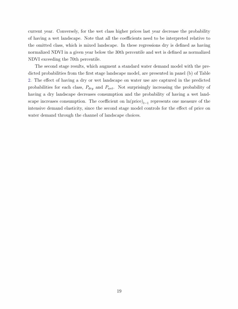
current year. Conversely, for the wet class higher prices last year decrease the probability
of having a wet landscape. Note that all the coefficients need to be interpreted relative to
the omitted class, which is mixed landscape. In these regressions dry is defined as having
normalized NDVI in a given year below the 30th percentile and wet is defined as normalized
NDVI exceeding the 70th percentile.
The second stage results, which augment a standard water demand model with the pre-
dicted probabilities from the first stage landscape model, are presented in panel (b) of Table
2. The effect of having a dry or wet landscape on water use are captured in the predicted
probabilities for each class, Pdry and Pwet. Not surprisingly increasing the probability of
having a dry landscape decreases consumption and the probability of having a wet land-
scape increases consumption. The coefficient on ln(price)t´1 represents one measure of the
intensive demand elasticity, since the second stage model controls for the effect of price on
water demand through the channel of landscape choices.
19

Table 2: Two Stage Model
(a) 1st Stage: LandscapeDry Wet
pricet´12 0.2428˚˚˚ -0.2303˚˚˚
(0.0043) (0.0038)Home Size -0.0076˚˚˚ 0.0283˚˚˚
(0.0019) (0.0018)Bedrooms -0.0006 0.0035
(0.0042) (0.0042)Year Built 3.8614˚˚˚ -5.6218˚˚˚
(0.1290) (0.1020)Pool 0.0058˚˚˚ -0.0094˚˚˚
(0.0006) (0.0006)House Price -0.0038˚˚ 0.0109˚˚˚
(0.0018) (0.0021)% Renters 0.0157˚˚˚ -0.0032˚˚˚
(0.0007) (0.0006)% College -0.0021 0.0655˚˚˚
(0.0015) (0.0017)Same House -0.0470˚˚˚ 0.0011
(0.0025) (0.0025)Number of Dry Neighbors 0.3678˚˚˚ -0.2071˚˚˚
(0.0013) (0.0007)House Sold 0.0010˚˚˚ -0.0007˚˚˚
(0.0001) (0.0001)Time Trend -0.0852˚˚˚ 0.0760˚˚˚
(0.0016) (0.0014)Households 171,081 171,081Observations 7,441,832 7,441,832
(b) 2nd Stage: Water DemandFirst Stage
ln(price)t´1 -0.2811˚˚˚
(0.0073)Pdry -0.0824˚˚˚
(0.0066)Pwet 0.0701˚˚˚
(0.0081)Time Trend -0.0135˚˚˚
(0.0004)Net ET 0.0048˚˚˚
(0.0002)Cooling Degree Days 0.0006˚˚˚
(0.0000)PHDI -0.0078˚˚˚
(0.0001)Household FEs YesHouseholds 171,073Observations 5,479,234
Note: Panel (a) presents the semi-elasticities from the first stage landscape multinomial logit model for both dry and wetcategories. The mixed category is the omitted category. The interpretation is the how a percentage change in the independentvariables affects the probability of being either dry or wet. Standard errors in the first stage model are computed by the deltamethod. The parameters for the second stage water demand model are presented in panel (b). The dependent variable is thenatural log of monthly water consumption; Pdry and Pwet are the probabilities for having dry or wet landscape in a given yearestimated in the first stage. The second stage standard errors are calculated using the bootstrap method where re-samplingtakes place at the household level. *** pă0.01, ** pă0.05, * pă0.1
4.2 Long Run Landscape AdoptionThe long run landscape adoption results are presented in three steps. First, I show
results from conditional demand regressions that isolate households that do not convert
their landscape and maintain either wet or dry landscapes. Second, I present the results of
a discrete choice model for the decision to convert landscape from wet to dry. Third, I show
how wet to dry landscape conversions impact water demand.
4.2.1 Conditional Demand Results
Table 3 presents the regression results from the conditional demand functions for the
three landscape groups: Mixed, Dry, and Wet. Since landscape remains constant for the
Dry and Wet groups, households in these groups can only change indoor water use and
the intensity of outdoor water use so the coefficients on price represent intensive margin
20
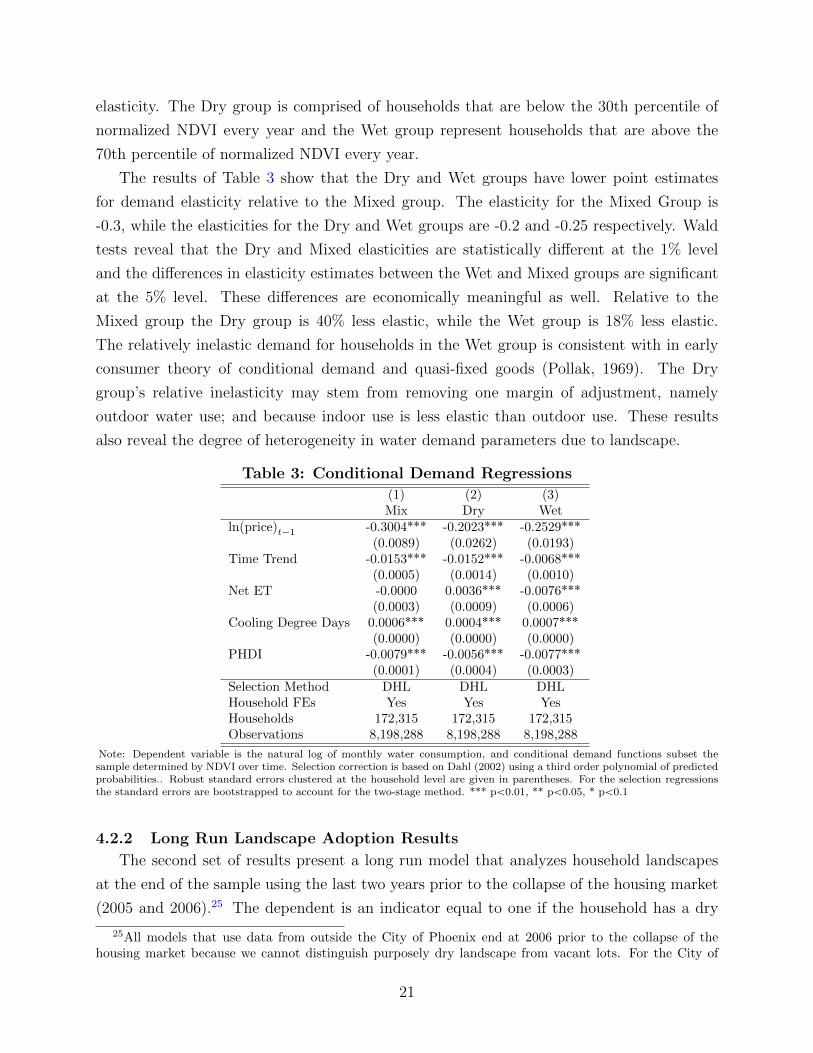
elasticity. The Dry group is comprised of households that are below the 30th percentile of
normalized NDVI every year and the Wet group represent households that are above the
70th percentile of normalized NDVI every year.
The results of Table 3 show that the Dry and Wet groups have lower point estimates
for demand elasticity relative to the Mixed group. The elasticity for the Mixed Group is
-0.3, while the elasticities for the Dry and Wet groups are -0.2 and -0.25 respectively. Wald
tests reveal that the Dry and Mixed elasticities are statistically different at the 1% level
and the differences in elasticity estimates between the Wet and Mixed groups are significant
at the 5% level. These differences are economically meaningful as well. Relative to the
Mixed group the Dry group is 40% less elastic, while the Wet group is 18% less elastic.
The relatively inelastic demand for households in the Wet group is consistent with in early
consumer theory of conditional demand and quasi-fixed goods (Pollak, 1969). The Dry
group’s relative inelasticity may stem from removing one margin of adjustment, namely
outdoor water use; and because indoor use is less elastic than outdoor use. These results
also reveal the degree of heterogeneity in water demand parameters due to landscape.
Table 3: Conditional Demand Regressions
(1) (2) (3)Mix Dry Wet
ln(price)t´1 -0.3004˚˚˚ -0.2023˚˚˚ -0.2529˚˚˚
(0.0089) (0.0262) (0.0193)Time Trend -0.0153˚˚˚ -0.0152˚˚˚ -0.0068˚˚˚
(0.0005) (0.0014) (0.0010)Net ET -0.0000 0.0036˚˚˚ -0.0076˚˚˚
(0.0003) (0.0009) (0.0006)Cooling Degree Days 0.0006˚˚˚ 0.0004˚˚˚ 0.0007˚˚˚
(0.0000) (0.0000) (0.0000)PHDI -0.0079˚˚˚ -0.0056˚˚˚ -0.0077˚˚˚
(0.0001) (0.0004) (0.0003)Selection Method DHL DHL DHLHousehold FEs Yes Yes YesHouseholds 172,315 172,315 172,315Observations 8,198,288 8,198,288 8,198,288
Note: Dependent variable is the natural log of monthly water consumption, and conditional demand functions subset thesample determined by NDVI over time. Selection correction is based on Dahl (2002) using a third order polynomial of predictedprobabilities.. Robust standard errors clustered at the household level are given in parentheses. For the selection regressionsthe standard errors are bootstrapped to account for the two-stage method. *** pă0.01, ** pă0.05, * pă0.1
4.2.2 Long Run Landscape Adoption Results
The second set of results present a long run model that analyzes household landscapes
at the end of the sample using the last two years prior to the collapse of the housing market
(2005 and 2006).25 The dependent is an indicator equal to one if the household has a dry
25All models that use data from outside the City of Phoenix end at 2006 prior to the collapse of thehousing market because we cannot distinguish purposely dry landscape from vacant lots. For the City of
21

landscape in the last two years of the sample. A linear probability model estimates the
probability of being dry based on long-run changes in water prices, utility rebate policies,
neighbors landscape choices, and the household’s initial landscape. The long run model
is only estimated on the Metro sample because there is no variation across households in
the long run differences in prices within a utility. Since there may be unobserved differences
across utilities other than prices and landscape rebates I use a boundary discontinuity design
that limits the sample to 1000 feet from a utility border when estimating models for the whole
metro area (Black, 1999; Ito, 2014).26
Table 4 shows the results of the long run dry landscape adoption model. I show three
results based on three definitions of conversions that vary the normalized NDVI threshold
for annual dry and wet landscape classifications. I relax the normalized NDVI thresholds for
wet and dry to above the 60th percentile and below the 40th percentile to more accurately
measure the number of conversions.27 First, wet is defined as above the 60th percentile
and dry as below the 40th percentile, which correspond to the results shown in Table 4. I
also define wet as above the 70th percentile and dry as below the 30th percentile. Lastly,
since the landscape groups are asymmetric (there are more households consistently wet than
consistently dry) I maintain the wet threshold at the 70th percentile and relax the dry
threshold to below the 40th percentile. Households are quite responsive in the long run,
which is 8 years. Increasing the maximum price by one dollar increases the probability of
having a dry landscape between 20-25% depending on the specification. Since this includes
households that started with, and maintained, dry landscapes the price effect is do to both
converting from wet to dry and maintaining a dry landscape.28 Additionally, introducing a
rebate for turf removal increases the probability of dry landscapes. The long run difference
in the proportion of neighbors with dry landscapes increases the probability of having a dry
landscape, as does the cumulative housing sales in a neighborhood. While the association
between neighbors’ conversions and a household’s conversion probability is intriguing, the
estimates should not be considered causal peer effects due to the issues of endogeneity raised
in Manski (1993, 2000).
Phoenix we know when lots are abandoned to the presence of water billing records.26Figure A.4 visualizes the boundary discontinuity approach and Table 9 shows estimates using a variety
of distance bandwidths.27The actual number of conversions is estimated to be roughly 20% based on analysis of aerial imagery
conducted by the City of Phoenix Water Department. Using the 60/40 thresholds 3.5% of households convertand using the 70/30 only 1% of the households convert. There are two primary reasons for the distinctionbetween the my estimates of conversions and the City of Phoenix’s estimates. First, the City of Phoenixclassifies any household that transitions from primarily turf grass as a conversion, even if they have somegreen landscape that may represent a high NDVI measure. Second, the City of Phoenix classifications donot track individual households over time but rely on repeated cross sections at different points in time.
28A model that excludes initially dry households yields similar qualitative results.
22

Table 4: Landscape Conversion(1) (2) (3)
60/40 70/30 70/40∆ Max Price 0.2012˚˚˚ 0.2466˚˚˚ 0.2291˚˚˚
(0.0211) (0.0246) (0.0234)∆ Rebate 0.0003 -0.0079 0.0015
(0.0219) (0.0251) (0.0245)Start Wet -0.5051˚˚˚ -0.3521˚˚˚ -0.4723˚˚˚
(0.0057) (0.0062) (0.0060)∆ Dry Neighbors 0.3043˚˚˚ 0.1394˚˚˚ 0.2236˚˚˚
(0.0194) (0.0206) (0.0207)ř
Sales 0.0080˚˚˚ 0.0082˚˚˚ 0.0105˚˚˚
(0.0019) (0.0020) (0.0020)Observations 86,901 86,901 86,901
Notes: The dependent variable in columns is an indicator equal to one if a household ends the sample with a dry landscape,defined as two consecutive annual low NDVI observations. The regressions use the Phoenix Metropolitan sample presentboundary discontinuity results that limit the sample to within 1000 feet of a utility border. The difference variables (∆)represent the differences from the last two years of the sample minus the first two years of the sample. Start Wet is a dummyequal to one if the household started the sample with two consecutive wet NDVI observations. The columns represent theNDVI percentile thresholds for an annual wet and dry classification, which are used to create the dependent variable (endingdry), Start Wet, and Dry Neighbors. Robust standard errors clustered at the census block level are reported in parentheses.*** pă0.01, ** pă0.05, * pă0.1
4.2.3 Landscape Conversions and Water Demand
The last component of the landscape conversion analysis estimates the change in water
consumption due to landscape conversions. Table 5 presents the results of the water demand
regression presented in equation 8 that includes the effect of conversions and neighbors’
conversions on water demand. Similar to Table 4 the columns show different NDVI thresholds
for annual landscape classification. All the results show that conversions have a negative
impact on water consumption magnitude that is not only statistically, but also economically,
significant at roughly 18-20% of monthly water demand. Neighbors’ conversions cause a
statistically significant reduction in demand, but the magnitude is roughly one tenth of that
for an actual household conversion. This is likely due to the fact that the probability of
converting increases when a household’s neighbors convert; therefore neighbors conversions
may act as a proxy for partial conversions that are not picked up by the NDVI data. The
results provide evidence from the water metering records that the satellite data are able to
capture landscape conversions. It should be noted that the effect of a landscape conversion
on water demand is only estimated with data from the Phoenix sample.
I calculate the long run arc elasticity of demand for the extensive by simulating the effect
of a 10% price increase on the probability of dry landscape adoption, and multiplying this
by the percentage change in consumption associated with a conversion (∆q “ ∆p ˆ γLR ˆ
δ1 ˆ Erw|wets). This captures the change in consumption due to price induced changes
in landscape. The long run extensive margin ranges from -.06 to -.09 depending on the
landscape classification thresholds used. I compare this to the intensive margin elasticity
23
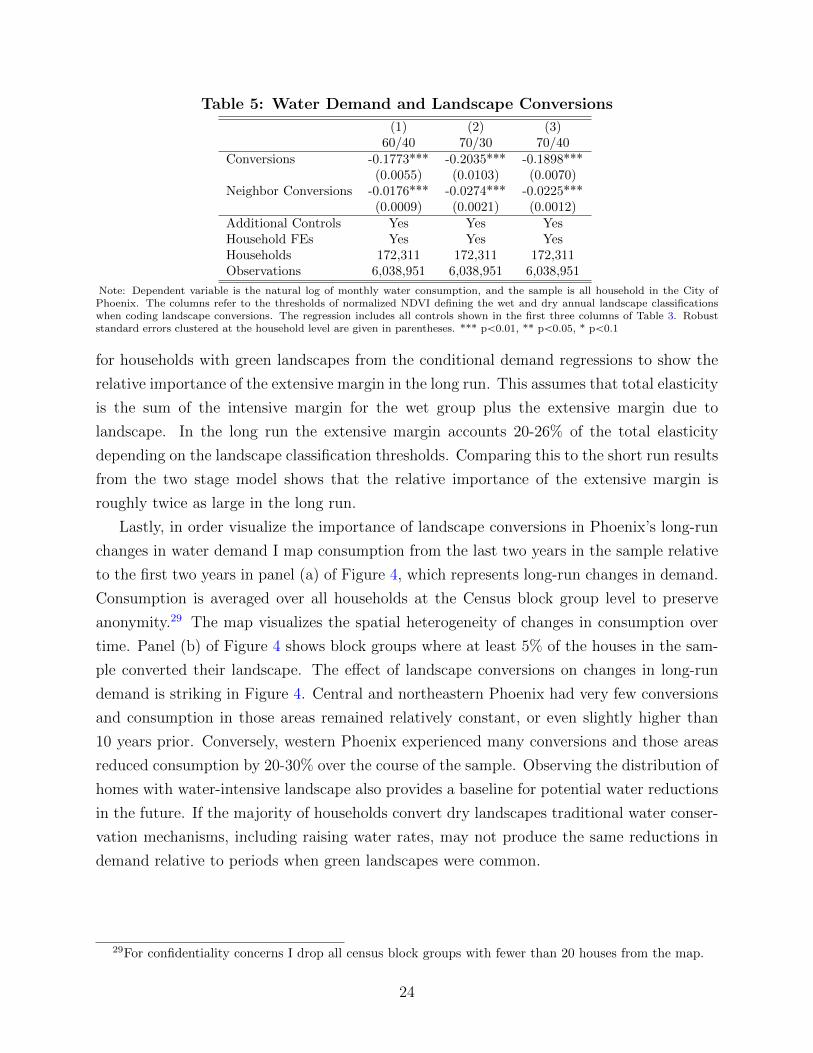
Table 5: Water Demand and Landscape Conversions
(1) (2) (3)60/40 70/30 70/40
Conversions -0.1773˚˚˚ -0.2035˚˚˚ -0.1898˚˚˚
(0.0055) (0.0103) (0.0070)Neighbor Conversions -0.0176˚˚˚ -0.0274˚˚˚ -0.0225˚˚˚
(0.0009) (0.0021) (0.0012)Additional Controls Yes Yes YesHousehold FEs Yes Yes YesHouseholds 172,311 172,311 172,311Observations 6,038,951 6,038,951 6,038,951
Note: Dependent variable is the natural log of monthly water consumption, and the sample is all household in the City ofPhoenix. The columns refer to the thresholds of normalized NDVI defining the wet and dry annual landscape classificationswhen coding landscape conversions. The regression includes all controls shown in the first three columns of Table 3. Robuststandard errors clustered at the household level are given in parentheses. *** pă0.01, ** pă0.05, * pă0.1
for households with green landscapes from the conditional demand regressions to show the
relative importance of the extensive margin in the long run. This assumes that total elasticity
is the sum of the intensive margin for the wet group plus the extensive margin due to
landscape. In the long run the extensive margin accounts 20-26% of the total elasticity
depending on the landscape classification thresholds. Comparing this to the short run results
from the two stage model shows that the relative importance of the extensive margin is
roughly twice as large in the long run.
Lastly, in order visualize the importance of landscape conversions in Phoenix’s long-run
changes in water demand I map consumption from the last two years in the sample relative
to the first two years in panel (a) of Figure 4, which represents long-run changes in demand.
Consumption is averaged over all households at the Census block group level to preserve
anonymity.29 The map visualizes the spatial heterogeneity of changes in consumption over
time. Panel (b) of Figure 4 shows block groups where at least 5% of the houses in the sam-
ple converted their landscape. The effect of landscape conversions on changes in long-run
demand is striking in Figure 4. Central and northeastern Phoenix had very few conversions
and consumption in those areas remained relatively constant, or even slightly higher than
10 years prior. Conversely, western Phoenix experienced many conversions and those areas
reduced consumption by 20-30% over the course of the sample. Observing the distribution of
homes with water-intensive landscape also provides a baseline for potential water reductions
in the future. If the majority of households convert dry landscapes traditional water conser-
vation mechanisms, including raising water rates, may not produce the same reductions in
demand relative to periods when green landscapes were common.
29For confidentiality concerns I drop all census block groups with fewer than 20 houses from the map.
24
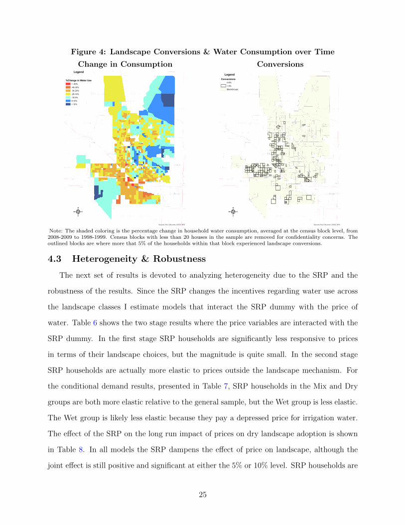
Figure 4: Landscape Conversions & Water Consumption over Time
Change in Consumption
Sources: Esri, DeLorme, USGS, NPS
4
Legend %Change in Water Use
< -40%-40-30%-30-20%-20-10%-10-0%0-10%> 10%
Conversions
Sources: Esri, DeLorme, USGS, NPS
4
LegendConversions
0-5%> 5%BlockGroups
Note: The shaded coloring is the percentage change in household water consumption, averaged at the census block level, from2008-2009 to 1998-1999. Census blocks with less than 20 houses in the sample are removed for confidentiality concerns. Theoutlined blocks are where more that 5% of the households within that block experienced landscape conversions.
4.3 Heterogeneity & Robustness
The next set of results is devoted to analyzing heterogeneity due to the SRP and the
robustness of the results. Since the SRP changes the incentives regarding water use across
the landscape classes I estimate models that interact the SRP dummy with the price of
water. Table 6 shows the two stage results where the price variables are interacted with the
SRP dummy. In the first stage SRP households are significantly less responsive to prices
in terms of their landscape choices, but the magnitude is quite small. In the second stage
SRP households are actually more elastic to prices outside the landscape mechanism. For
the conditional demand results, presented in Table 7, SRP households in the Mix and Dry
groups are both more elastic relative to the general sample, but the Wet group is less elastic.
The Wet group is likely less elastic because they pay a depressed price for irrigation water.
The effect of the SRP on the long run impact of prices on dry landscape adoption is shown
in Table 8. In all models the SRP dampens the effect of price on landscape, although the
joint effect is still positive and significant at either the 5% or 10% level. SRP households are
25

also less responsive to the introduction of turf rebates.
Table 6: Two Stage Model with SRP Interaction
(a) 1st Stage: LandscapeDry Wet
pricet´12 0.2450˚˚˚ -0.2482˚˚˚
(0.0044) (0.0038)pricet´12*SRP -0.0029˚˚˚ 0.0248˚˚˚
(0.0008) (0.0009)Additional Controls Yes YesHouseholds 171,081 171,081Observations 7,441,832 7,441,832
(b) 2nd Stage: Water DemandFirst Stage
ln(price)t´1 -0.2492˚˚˚
(0.0080)ln(price)t´1*SRP -0.0694˚˚˚
(0.0065)Pdry -0.0723˚˚˚
(0.0066)Pwet 0.0706˚˚˚
(0.0084)Household FEs YesAdditional Controls YesHouseholds 171,073Observations 5,479,234
Note: Panel (a) presents the semi-elasticities from the first stage landscape multinomial logit model for both dry and wetcategories. The mixed category is the omitted category. The interpretation is the how a percentage change in the independentvariables affects the probability of being either dry or wet. Standard errors in the first stage model are computed by the deltamethod. The parameters for the second stage water demand model are presented in panel (b). The dependent variable is thenatural log of monthly water consumption; p(Dry) and p(Wet) are the probabilities for having dry or wet landscape in a givenyear estimated in the first stage. The second stage standard errors are calculated using the bootstrap method where re-samplingtakes place at the household level. Both models include all parameters that are shown in Table 2. Those parameters are omittedfor space concerns and are available upon request *** pă0.01, ** pă0.05, * pă0.1
Table 7: Conditional Demand Regressions with SRP Interaction
(1) (2) (3)Mix Dry Wet
ln(price)t´1 -0.2412˚˚˚ -0.1587˚˚˚ -0.3439˚˚˚
(0.0100) (0.0264) (0.0223)ln(price)t´1*SRP -0.1305˚˚˚ -0.1331˚˚˚ 0.1247˚˚˚
(0.0067) (0.0232) (0.0187)Selection Method DHL DHL DHLHousehold FEs Yes Yes YesAdditional Controls Yes Yes YesHouseholds 172,315 172,315 172,315Observations 8,198,288 8,198,288 8,198,288
Note: Dependent variable is the natural log of monthly water consumption, and conditional demand functions subset thesample determined by NDVI over time. Selection correction is based on a flexible version of Dubin and McFadden (1984). Themodels include all parameters that are shown in Table 3. Those parameters are omitted for space concerns and are availableupon request. The standard errors are bootstrapped to account for the two-stage method. *** pă0.01, ** pă0.05, * pă0.1
The next set of results examines the robustness of the results. First, I replicate the two
stage model after changing the NDVI percentile thresholds for wet and dry classifications to
above the 80th and below the 20th percentiles, as well as above the 80th and below the 30th.
The results are qualitatively similar and are presented in the Appendix in Tables A.5 and A.6.
I repeat this same exercise with the conditional demand functions, presented in Tables A.7
26
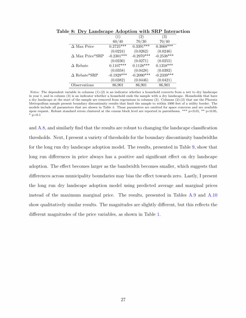
Table 8: Dry Landscape Adoption with SRP Interaction(1) (2) (3)
60/40 70/30 70/40∆ Max Price 0.2725˚˚˚ 0.3391˚˚˚ 0.3068˚˚˚
(0.0224) (0.0262) (0.0246)∆ Max Price*SRP -0.2301˚˚˚ -0.2970˚˚˚ -0.2538˚˚˚
(0.0230) (0.0271) (0.0255)∆ Rebate 0.1107˚˚˚ 0.1128˚˚˚ 0.1358˚˚˚
(0.0358) (0.0428) (0.0392)∆ Rebate*SRP -0.1929˚˚˚ -0.2090˚˚˚ -0.2339˚˚˚
(0.0382) (0.0446) (0.0421)Observations 86,901 86,901 86,901
Notes: The dependent variable in columns (1)-(2) is an indicator whether a household converts from a wet to dry landscapein year t, and in column (3) is an indicator whether a household ends the sample with a dry landscape. Households that havea dry landscape at the start of the sample are removed from regressions in columns (2). Columns (2)-(3) that use the PhoenixMetropolitan sample present boundary discontinuity results that limit the sample to within 1000 feet of a utility border. Themodels include all parameters that are shown in Table 4. Those parameters are omitted for space concerns and are availableupon request. Robust standard errors clustered at the census block level are reported in parentheses. *** pă0.01, ** pă0.05,* pă0.1
and A.8, and similarly find that the results are robust to changing the landscape classification
thresholds. Next, I present a variety of thresholds for the boundary discontinuity bandwidths
for the long run dry landscape adoption model. The results, presented in Table 9, show that
long run differences in price always has a positive and significant effect on dry landscape
adoption. The effect becomes larger as the bandwidth becomes smaller, which suggests that
differences across municipality boundaries may bias the effect towards zero. Lastly, I present
the long run dry landscape adoption model using predicted average and marginal prices
instead of the maximum marginal price. The results, presented in Tables A.9 and A.10
show qualitatively similar results. The magnitudes are slightly different, but this reflects the
different magnitudes of the price variables, as shown in Table 1.
27

Table 9: Boundary Bandwidths for Landscape Conversion ModelsAll 3000ft 2500ft 2000ft 1500ft 1000ft 500ft
∆ Max Price 0.0583˚˚˚ 0.1542˚˚˚ 0.1650˚˚˚ 0.1840˚˚˚ 0.2133˚˚˚ 0.2466˚˚˚ 0.3592˚˚˚
(0.0132) (0.0156) (0.0168) (0.0186) (0.0212) (0.0246) (0.0323)∆ Rebate 0.0135 0.0293˚ 0.0206 0.0011 0.0011 -0.0079 0.0019
(0.0148) (0.0150) (0.0156) (0.0171) (0.0198) (0.0251) (0.0344)Additional Controls Yes Yes Yes Yes Yes Yes YesObservations 370,781 213,985 191,084 159,057 126,119 86,901 42,478
Notes: The dependent variable is an indicator whether a household converts from a wet to dry landscape in year t. Thecolumns show different different bandwidths for the boundary discontinuity analysis using observations from all of the PhoenixMetropolitan area. Column (1) (All) shows the results for the full sample. Households that have a dry landscape at the start ofthe sample are removed. The models include all parameters that are shown in Table 4. Those parameters are omitted for spaceconcerns and are available upon request. Robust standard errors clustered at the census block level are reported in parentheses.*** pă0.01, ** pă0.05, * pă0.1
5 Conclusion
This paper examines the role of landscape choice in water demand by merging a time series
of satellite data with monthly water metering records. Jointly observing water demand and
changes in complementary goods over time enables estimation of demand elasticity on the
intensive and extensive margin. As concerns of water scarcity increase it is critical to develop
a deeper understanding of demand, particularly the role of complementary goods, as seen
in energy economics (Gillingham, 2012; Goulder et al., 2009). I examine the heterogeneity
in water demand due to an important complementary good by conditioning on landscape
decisions over time. Key differences exist between households across the landscape spectrum.
Households that maintain a dry landscape are less elastic than the general population.
I find that higher water rates increase the probability of adopting a water-efficient land-
scape in both the short run and the long run. This is robust across a range of price and land-
scape specifications as well as controlling for utility specific unobservables with a boundary
discontinuity analysis. Landscape conversions have a significant impact on demand; reducing
consumption by roughly 20%. Changes along the extensive margin constitute only 10% of
aggregate demand elasticity in the short run, and this rises to 20-26% in the long run. There
appears to be a strong social component to the landscape choice, as neighbors’ conversions
are a strong predictor of a household’s decision to switch to a water saving landscape. As
social norms evolve, and consumers sort to live near like-minded people or collocate along
28

correlated unobserved heterogeneity, the pattern of conversion clusters is likely to continue.
There are important implications for clusters of conversions in a desert city as xeric land-
scapes nonlinearly exacerbate the urban heat island. Establishing xeric landscapes may lead
to a tradeoff between water and energy conservation as hotter neighborhoods use more en-
ergy for cooling (Klaiber et al., 2017). This highlights the notion that a green landscape
provides both direct benefits and indirect benefits in arid regions.
Analyzing long-run changes in demand reveals that households maintaining a green land-
scape have a relatively constant trend in consumption over time, while areas that convert
appear to be driving large scale reductions in demand. If, as expected, the transition of
landscaping practices in the Phoenix metropolitan area leads to increases in xeric landscape
there will be important implications for water demand. There will be smaller peaks in sum-
mer demand and, since dry households are less price elastic, aggregate demand elasticity will
also decrease. Thus, conversions to dry landscapes smooth seasonal water consumption, but
also reduce the potential savings from price increases and outdoor water restrictions during
droughts. Grass and other types of water intensive landscapes act as an additional source
of supply that can be drawn down during times of drought through reductions in irrigation.
As cities in arid climates transition from towards more xerix landscapes they lose the ability
to quickly reduce consumption during a drought. Understanding the stock of existing land-
scape, and the drivers of conversion, has enormous consequences for long and medium run
planning by quantifying the potential savings from outdoor use.
29

ReferencesAggarwal, Rimjhim M., Subhrajit Guhathakurta, Susanne Grossman-Clarke,
and Vasudha Lathey, “How do variations in Urban Heat Islands in space and timeinfluence household water use? The case of Phoenix, Arizona,” Water Resources Research,June 2012, 48 (6), 1–13.
Allcott, Hunt and Nathan Wozny, “Gasoline prices, fuel economy, and the energyparadox,” Review of Economics and Statistics, 2014, 96 (5), 779–795.
Baerenklau, Kenneth A, Kurt A Schwabe, and Ariel Dinar, “The residential waterdemand effect of increasing block rate water budgets,” Land Economics, 2014, 90 (4),683–699.
Balling, R. C., P. Gober, and N. Jones, “Sensitivity of residential water consumptionto variations in climate: An intraurban analysis of Phoenix, Arizona,” Water ResourcesResearch, October 2008, 44 (10), 1–11.
Bell, David R and Ronald C Griffin, “Urban Water Demand with Periodic Error Cor-rection,” Land Economics, 2011, 87 (3), 528–544.
Billings, R Bruce and Donald E Agthe, “Price Elasticities for Water: A Case ofIncreasing Block Rates,” Land Economics, 1980, 56 (1), 73–84.
Biørn, Erik, Rolf Golombek, and Arvid Raknerud, “Environmental Regulations andPlant Exit,” Environmental and Resource Economics, 1998, 11, 35–59.
Black, Sandra E, “Do better schools matter? Parental valuation of elementary education,”Quarterly Journal of Economics, 1999, pp. 577–599.
Brelsford, Christa and Joshua K Abbott, “How Smart Are ’Water Smart Land-scapes’?,” arXiv preprint arXiv:1803.04593, 2018.
Brent, Daniel A, Joseph H Cook, and Skylar Olsen, “Social comparisons, householdwater use, and participation in utility conservation programs: Evidence from three ran-domized trials,” Journal of the Association of Environmental and Resource Economists,2015, 2 (4), 597–627.
Buck, Steven, Maximilian Auffhammer, Stephen Hamilton, and David Sunding,“Measuring welfare losses from urban water supply disruptions,” Journal of the Associa-tion of Environmental and Resource Economists, 2016, 3 (3), 743–778.
Busse, Meghan R, Christopher R Knittel, and Florian Zettelmeyer, “Are con-sumers myopic? Evidence from new and used car purchases,” American Economic Review,2013, 103 (1), 220–56.
Butsic, Van, David J Lewis, and Lindsay Ludwig, “An Econometric Analysis of LandDevelopment with Endogenous Zoning,” Land Economics, 2011, 87 (3), 412–432.
Carver, Philip H. and John J. Boland, “Short- and long-run effects of price on municipalwater use,” Water Resources Research, 1980, 16 (4), 609.
Chamberlain, Gary, “Multivariate Regression Models For Panel Data,” Journal of Econo-metrics, 1982, 18, 5–42.
Chavez, Pat S, “Image-Based Atmospheric Corrections - Revisited and Improved,” Pho-togrammetric engineering and remote sensing, 1996, 62 (9), 1025–1036.
Dahl, Gordon B, “Mobility and the Return to Education: Testing a Roy Model withMultiple Markets,” Econometrica, 2002, 70 (6), 2367–2420.
Dalhuisen, Jasper M., Raymond J. G. M. Florax, Henri L. F. de Groot, and
30

Peter Nijkamp, “Price and Income Elasticities of Residential Water Demand: A Meta-Analysis,” Land Economics, May 2003, 79 (2), 292.
Dandy, Graeme, Tin Nguyen, and Carolyn Davies, “Estimating Residential WaterDemand in the Presence of Free Allowances,” Land Economics, 1997, 73 (1), 125–139.
Dubin, Jeffery A. and Daniel L. McFadden, “An Econometric Analysis of ResidentialElectric Appliance Holdings and Consumption,” Econometrica, 1984, 52 (2), 345–362.
Espey, M., J. Espey, and W. D. Shaw, “Price elsasticity of residential demand forwater: A meta-analysis,” Water Resources Research, 1997, 33 (6), 1369–1374.
Farzi, Y. H., K. J. M. Huisman, and P. M. Kort, “Optimal timing of technologyadoption,” Journal of Economic Dynamics and Control, 1998, 22, 779–799.
Ferraro, Paul J and Michael K Price, “Using nonpecuniary strategies to influence be-havior: evidence from a large-scale field experiment,” Review of Economics and Statistics,2013, 95 (1), 64–73.
Gillingham, Kenneth, “Selection on Anticipated Driving and the Consumer Response toChanging Gasoline Prices,” 2012.
, “Identifying the Elasticity of Driving: Evidence from a Gasoline Price Shock in Califor-nia,” Regional Science and Urban Economics, July 2014, 47 (4), 13–24.
Gitelson, Anatoly A, “Remote estimation of crop fractional vegetation cover: the useof noise equivalent as an indicator of performance of vegetation indices,” InternationalJournal of Remote Sensing, 2013, 34 (17), 6054–6066.
Goulder, Lawrence H., Antonio M. Bento, Mark R. Jacobsen, and Roger H.von Haefen, “Distributional and Efficiency Impacts of Increased US Gasoline Taxes,”American Economic Review, 2009, 99 (3), 667–699.
Grafton, R. Quentin and Michael B. Ward, “Prices versus Rationing: MarshallianSurplus and Mandatory Water Restrictions*,” Economic Record, September 2008, 84(September 2008), S57–S65.
Hanemann, W. Michael, “Discrete/Continuous Models of Consumer Demand,” Econo-metrica, 1984, 52 (3), 541–561.
Hassett, Kevin A. and Gilbert E. Metcalf, “Energy tax credits and residential conser-vation investment: Evidence from panel data,” Journal of Public Economics, June 1995,57 (2), 201–217.
Heckman, James, “Shadow Prices , Market Wages , and Labor Supply,” Econometrica,1974, 42 (4), 679–694.
Hewitt, Julie A. and Michael W. Hanemann, “A Discrete/Continuous Choice Ap-proach to Residential Water Demand under Block Rate Pricing,” Land Economics, 1995,71 (2), 173–192.
Huete, A R, H Q Liu, K Batchily, and W Van Leeuwen, “A Comparison of Veg-etation Indices over a Global Set of TM Images for EOS-MODIS,” Remote Sensing ofEnvironment, 1997, 59, 440–451.
Ito, Koichiro, “Do Consumers Respond to Marginal or Average Price? Evidence fromNonlinear Electricity Pricing,” American Economic Review, February 2014, 104 (2), 537–563.
Klaiber, H Allen, Joshua K Abbott, and V Kerry Smith, “Some Like It (Less)Hot: Extracting Trade-Off Measures for Physically Coupled Amenities,” Journal of the
31

Association of Environmental and Resource Economists, 2017, 4 (4), 1053–1079.
, V Kerry Smith, Michael Kaminsky, and Aaron Strong, “Measuring price elas-ticities for residential water demand with limited information,” Land Economics, 2014, 90(1), 100–113.
Manski, Charles F., “Identification of Endogenous Social Effects: The Reflection Prob-lem,” The Review of Economic Studies, July 1993, 60 (3), 531.
Manski, Charles F, “Economic Analysis of Social Interactions,” Journal of EconomicPerspectives, August 2000, 14 (3), 115–136.
Mansur, Erin T. and Sheila M. Olmstead, “The value of scarce water: Measuring theinefficiency of municipal regulations,” Journal of Urban Economics, May 2012, 71 (3),332–346.
Mundlak, Yair, “On the Pooling of Time Series and Cross Sectino Data,” Econometrica,1978, 46 (1), 69–85.
Myint, Soe W, May Yuan, Randall S Cerveny, and Chandra P Giri, “Comparisonof Remote Sensing Image Processing Techniques to Identify Tornado Damage Areas fromLandsat TM Data,” Sensors, 2008, 8, 1128–1156.
Nataraj, Shanthi and W. Michael Hanemann, “Does marginal price matter? A re-gression discontinuity approach to estimating water demand,” Journal of EnvironmentalEconomics and Management, March 2011, 61 (2), 198–212.
Nauges, Celine and Alban Thomas, “Long-run Study of Residential Water Consump-tion,” Environmental and Resource Economics, 2003, 26, 25–43.
Newell, Richard G and Juha Siikamaki, “Nudging energy efficiency behavior: Therole of information labels,” Journal of the Association of Environmental and ResourceEconomists, 2014, 1 (4), 555–598.
Nieswiadomy, Michael L and David J. Molina, “Comparing Residential Water DemandEstimates under Decreasing and Increasing Block Rates Using Household Data,” LandEconomics, 1989, 65 (3), 280–289.
Olmstead, Sheila M., W. Michael Hanemann, and Robert N. Stavins, “Waterdemand under alternative price structures,” Journal of Environmental Economics andManagement, September 2007, 54 (2), 181–198.
Perry, Christopher J, CJ Perry, Michael Rock, D Seckler, Michael T Rock, andDavid William Seckler, Water as an economic good: A solution or a problem?, Vol. 14,IWMI, 1997.
Pint, Ellen M, “Household Responses to Increased Water Rates during the ColiforniaDrought,” Land Economics, 1999, 75 (2), 246–266.
Pollak, R.A., “Conditional demand functions and consumption theory,” The QuarterlyJournal of Economics, 1969, 83 (1), 60–78.
Revelt, David and Kenneth Train, “Mixed Logit with Repeated Choices: Households’Choices of Appliance Efficiency Level,” Review of Economics and Statistics, November1998, 80 (4), 647–657.
Schatzki, Todd, “Options, uncertainty and sunk costs: an empirical analysis of land usechange,” Journal of Environmental Economics and Management, July 2003, 46 (1), 86–105.
Shin, Jeong-Shik, “Perception of Price When Price Information is Costly: Evidence from
32

Residential Electricity Demand,” The Review of Economics and Statistics, 1985, 67 (4),591–598.
Sovocool, Kent A, Mitchell Morgan, and Doug Bennett, “An in-depth investiaga-tion of Xeriscape as a water conservation measure,” Journal of American Water WorksAssociation, 2006, 98 (2), 82–93.
Stefanov, William L. and Maik Netzband, “Assessment of ASTER land cover andMODIS NDVI data at multiple scales for ecological characterization of an arid urbancenter,” Remote sensing of Environment, 2005, 99 (1-2), 31–43.
, Michael S. Ramsey, and Philip R. Christensen, “Monitoring urban land coverchange: An expert system approach to land cover classification of semiarid to arid urbancenters,” Remote Sensing of Environment, 2001, 77 (2), 173–185.
Tchigriaeva, Elena, Corey Lott, and Rollins Kimberly, “Modeling effects of multipleconservation policy instruments and exogenous factors on urban residential water demandthrough household heterogeneity,” 2014.
Vaage, Kjell, “Heating technology and energy use: a discrete/continuous choice approachto Norwegian household energy demand,” Energy Economics, 2000, 22 (6), 649–666.
Vina, Andres, Anatoly a. Gitelson, Anthony L. Nguy-Robertson, and Yi Peng,“Comparison of different vegetation indices for the remote assessment of green leaf areaindex of crops,” Remote Sensing of Environment, December 2011, 115 (12), 3468–3478.
Wentz, Elizabeth A. and Patricia Gober, “Determinants of Small-Area Water Con-sumption for the City of Phoenix, Arizona,” Water Resources Management, February2007, 21 (11), 1849–1863.
Wichman, Casey J., “Perceived price in residential water demand: Evidence from a nat-ural experiment,” Journal of Economic Behavior & Organization, 2014, pp. 1–16.
Wichman, Casey J, Laura O Taylor, and Roger H Von Haefen, “Conservation poli-cies: Who responds to price and who responds to prescription?,” Journal of EnvironmentalEconomics and Management, 2016, 79, 114–134.
Woolridge, Jefferey M., Econometric Analysis of Cross Section and Panel Data, Cam-bridge, MA: MIT Press, 2002.
33
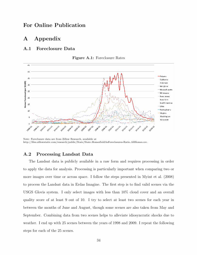
For Online Publication
A Appendix
A.1 Foreclosure Data
Figure A.1: Foreclosure Rates
Note: Foreclosure data are from Zillow Research, available athttp://files.zillowstatic.com/research/public/State/State HomesSoldAsForeclosures-Ratio AllHomes.csv.
A.2 Processing Landsat Data
The Landsat data is publicly available in a raw form and requires processing in order
to apply the data for analysis. Processing is particularly important when comparing two or
more images over time or across space. I follow the steps presented in Myint et al. (2008)
to process the Landsat data in Erdas Imagine. The first step is to find valid scenes via the
USGS Glovis system. I only select images with less than 10% cloud cover and an overall
quality score of at least 9 out of 10. I try to select at least two scenes for each year in
between the months of June and August, though some scenes are also taken from May and
September. Combining data from two scenes helps to alleviate idiosyncratic shocks due to
weather. I end up with 25 scenes between the years of 1998 and 2009. I repeat the following
steps for each of the 25 scenes.
34

Since the Landsat data is stored in separate bands I import the data and stack all
the layers on top of each other. Next, I subset the image to limit the geographic area to
Phoenix metro. Each Landsat scene is 185km x 117km so limiting the image to the study
area greatly increases computational speed and the digital space required for storage. Each
image is registered to a base image in order to reduce locational errors using 14 ground
control points and ensuring root mean squared errors of less than 0.1. This process ensures
that all the images align properly and that a parcel has the same geo-reference in each image
over time. In order to account for differences in atmospheric reflectance and solar radiation
I apply the Cos(t) method of radiometric correction of Chavez (1996). Once theses steps are
complete the images are suitable to be compared over time and I calculate the Normalized
Difference Vegetation Index (NDVI).
The Landsat satellite captures reflected and emitted energy in six bands of the electro-
magnetic spectrum as well as one thermal band. Landsat TM5 takes an image of the same
location every 16 days with 30-meter resolution, but is often obstructed by clouds, rendering
the image unusable. In the remote sensing literature there is a debate over the best index to
measure vegetative cover see among others (Gitelson, 2013; Huete et al., 1997; Vina et al.,
2011). NDVI is widely used and is appropriate as an introduction to incorporating remote
sensing data into water demand. NDVI is the calculated from the visible and near-infrared
bands in the Landsat data.30 Healthy green vegetation absorbs visible light and reflects
infrared light so the difference performs well in identifying healthy vegetation. The formula
used to calculate the index is NDV I “ pNIR ´ V ISq{pNIR ` V ISq, where NIR is the
near infrared band and V IS is the visible red band. This formula results in an index ranging
from -1 to 1 with higher values representing more robust vegetation. Figure A.2 shows an
area just northwest of Arizona State University to give an example of how different values
of NDVI correspond to land use features.
The NDVI data are then merged with parcel boundaries in Geographic Information Sys-
30More information on NDVI is available athttp://earthobservatory.nasa.gov/Features/MeasuringVegetation/measuring vegetation 2.php.
35

Figure A.2: NDVI of Known Land Features
Water
Golf Course
Highway NDVI = -0.58
NDVI = 0.14
NDVI = 0.778
Note: This is a sample area just northwest of Arizona State University, whose land usefeatures are known.
tem software. Each pixel of the Landsat data is 30m x 30m and is often larger, or matches
imperfectly, with the parcel boundaries. The size of each Landsat pixel is 900m2, which is
slightly larger than the average lot size of 861m2. An example of the problems that can arise
from merging NDVI at the parcel level are displayed in Figure A.3. It is clear that smaller
parcels create challenges for spatially merging NDVI data. To reduce the noise in the spatial
merge I downscale each NDVI pixel to nice 10m x 10m pixels and take the spatially weighted
average of the pixels within the parcel. The final results is a panel dataset at the parcel level
that contains the time series variation of NDVI for each of the 25 Landsat scenes.
A.3 Weather Normalization
While the processing steps described above alleviates concerns due fluctuations over time
in how the satellite captures images, I also need to account for the impact of natural variations
in weather on NDVI. Irrespective of human watering practices NDVI will vary based on the
weather conditions in the area. In order to minimize these variations and focus on the water-
added component of landscape I normalize the NDVI for weather. Since the images are taken
at different times of the month I match daily weather data based on the image date. From
this I construct variables representing weather conditions for each of the four weeks prior to
the image. Since Phoenix is very dry and often will not have rained within four weeks in the
36

Figure A.3: Merging Parcels and NDVI
Note: The color gradient for the images is the same, but is purely for illustrative purposes.Each pixel is 900m2 and is actually composed of nine 100m2 homogeneous pixels that improvethe spatially weighted average of parcel-level NDVI.
summer I generate a variable for the number of days since the last precipitation event. Next
I regress NDVI on these weather variables and keep the residuals as weather-normalized
values of NDVI.
Table A.1 presents the results of the weather normalizations with lags of up to four
weeks. I select residuals from the regression in column (4) as my preferred measure, though
robustness checks using other normalizations produce very similar results. The results in
Table A.1 are mostly intuitive with the cumulative effect of higher soil temperatures and
evapotranspiration leading to lower values of NDVI. Net precipitation increases NDVI and
the longer dry periods decrease NDVI. Overall weather explains between 10-14% of NDVI
suggesting that most of the variation is spatial, due to different landscaping practices across
the city. The regressions maintain the spatial variation because analyzing the residuals shows
that the standard deviation in normalized NDVI within a given year is very similar to the
standard deviation of the raw data.
37
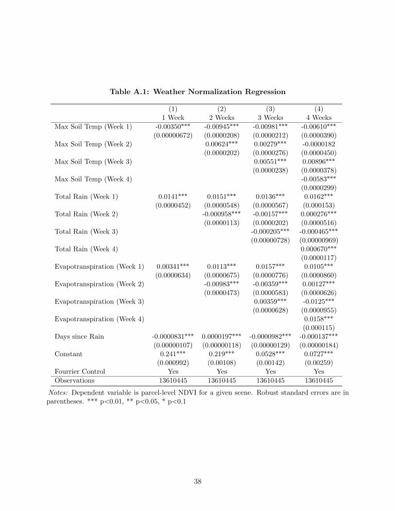
Table A.1: Weather Normalization Regression
(1) (2) (3) (4)1 Week 2 Weeks 3 Weeks 4 Weeks
Max Soil Temp (Week 1) -0.00350˚˚˚ -0.00945˚˚˚ -0.00981˚˚˚ -0.00610˚˚˚
(0.00000672) (0.0000208) (0.0000212) (0.0000390)Max Soil Temp (Week 2) 0.00624˚˚˚ 0.00279˚˚˚ -0.0000182
(0.0000202) (0.0000276) (0.0000450)Max Soil Temp (Week 3) 0.00551˚˚˚ 0.00896˚˚˚
(0.0000238) (0.0000378)Max Soil Temp (Week 4) -0.00583˚˚˚
(0.0000299)Total Rain (Week 1) 0.0141˚˚˚ 0.0151˚˚˚ 0.0136˚˚˚ 0.0162˚˚˚
(0.0000452) (0.0000548) (0.0000567) (0.000153)Total Rain (Week 2) -0.000958˚˚˚ -0.00157˚˚˚ 0.000276˚˚˚
(0.0000113) (0.0000202) (0.0000516)Total Rain (Week 3) -0.000205˚˚˚ -0.000465˚˚˚
(0.00000728) (0.00000969)Total Rain (Week 4) 0.000670˚˚˚
(0.0000117)Evapotranspiration (Week 1) 0.00341˚˚˚ 0.0113˚˚˚ 0.0157˚˚˚ 0.0105˚˚˚
(0.0000634) (0.0000675) (0.0000776) (0.0000860)Evapotranspiration (Week 2) -0.00983˚˚˚ -0.00359˚˚˚ 0.00127˚˚˚
(0.0000473) (0.0000583) (0.0000626)Evapotranspiration (Week 3) 0.00359˚˚˚ -0.0125˚˚˚
(0.0000628) (0.0000955)Evapotranspiration (Week 4) 0.0158˚˚˚
(0.000115)Days since Rain -0.0000831˚˚˚ 0.0000197˚˚˚ -0.0000982˚˚˚ -0.000137˚˚˚
(0.00000107) (0.00000118) (0.00000129) (0.00000184)Constant 0.241˚˚˚ 0.219˚˚˚ 0.0528˚˚˚ 0.0727˚˚˚
(0.000992) (0.00108) (0.00142) (0.00259)Fourrier Control Yes Yes Yes Yes
Observations 13610445 13610445 13610445 13610445
Notes: Dependent variable is parcel-level NDVI for a given scene. Robust standard errors are inparentheses. *** pă0.01, ** pă0.05, * pă0.1
38

A.4 Landscape Classification Diagnostics
In order to test the feasibility of using NDVI to classify different landscape varieties I
compare the quantiles of NDVI to data from a widely cited remote sensing paper. Stefanov
et al. (2001) classifies 11 different types of land use for Phoenix using 1998 data, including
mesic and xeric residential. I merge the parcels with 1998 NDVI with the classification
from Stefanov et al. (2001) keeping all parcels identified as either mesic or xeric. Table A.2
presents the percentage of parcels that were correctly identified as either mesic or xeric using
various quantiles of NDVI. The columns show the thresholds for NDVI quantiles to make
a classification. Parcels with NDVI above the higher threshold are classified as wet in a
given year and parcels with NDVI less than the low threshold are defined as dry. Therefore
decreasing the high threshold and increasing the low threshold relaxes the conditions to
observe a conversion. NDVI does a relatively better job classifying dry landscapes and for
that reason I use an asymmetric threshold for defining landscape groups For example in
the conditional demand models I designate a the Wet group by households that have NDVI
above the 80th quantile every year, and the Dry group by households that have below the
30th quantile every year. The results in Table A.2 contribute to establishing a relatively less
stringent threshold for the Dry group.
Table A.2: Landscape Diagnostics
NDVI Quantiles 90/10 80/20 70/30 60/40
% CorrectWet 77% 71% 67% 64%Dry 94% 90% 88% 85%
Notes: The columns designate the quantile of NDVI to compare with wet and dry landscapes. Thehigher quantile is used to determine wet parcels and the lower quantile designates dry parcels. Thepercentage correct takes the data from Stefanov et al. (2001) as the true value. We only comparesingle family residential households that were classified as xeric or mesic.
39

A.5 Water Demand Specification
Before estimating the conditional demand functions I perform model specification based
on the full sample pooled over all landscapes by estimating the water demand function
presented in equation (2).
lnpwitq “ αi ` γlnppitq ` βX1it ` ξit (9)
Here wit is water consumption for household i at time t, pw,it is the price of water, Xit
is vector weather controls, αi is a household level fixed effect, and ξit is an idiosyncratic
error term. The dependent variable is the log of monthly water consumption, with panel
cluster-robust standard errors at the household level as defined by Woolridge (2002).31
I run three specifications of the price in the water demand function: marginal price,
average price, the high marginal price. Due to the increasing block rate structure of water
rates the marginal and average price that a consumer faces depends on how much water
she chooses to consume, creating a simultaneity problem when estimating demand functions
(Hanemann, 1984; Hewitt and Hanemann, 1995; Nieswiadomy and Molina, 1989). A common
approach to deal with the endogeneity is to use the full rate structure (fixed cost, low block
price, and high block price) as instruments since the variables are correlated with actual
marginal price and exogenous to the household (Nieswiadomy and Molina, 1989; Olmstead
et al., 2007). In all specifications the dependent variable is the natural log of monthly
household water consumption, as there is strong evidence that water demand is distributed
log normally. I also run all three price specifications using one month lagged prices in case
consumers change current consumption in response to the previous bill.
Table A.3 presents the results from the water demand specification regressions. A 2SLS
model is used to estimate demand for columns (1), (3), (4), and (6), and Columns (2)
31A cluster-robust version of the Hausman test for the random effects versus fixed effects (Mundlak, 1978;Chamberlain, 1982; Woolridge, 2002) for each model in Table A.3 rejects the null of no correlation, requiringthe fixed effects model.
40
and (5) estimates a feasible generalized least squares model. Net evapotranspiratin (ET)
is the consumptive water requirement for turf grass minus the observed precipitation in
millimeters per square foot. Cooling degree days are the monthly sum of daily differences
between maximum temperature and 65 degrees Fahrenheit. PHDI is the Palmer Hydrological
Drought Index that serves as a proxy for medium to long-run drought conditions with lower
values signifying more severe droughts. Comparing the results across specifications, the
estimates for price elasticity range from -0.24 to -0.31 for the contemporaneous price, which
is in the range of conventional estimates (Espey et al., 1997; Dalhuisen et al., 2003). The
models that use lagged coefficients produce less elastic estimates that range from -0.20 to
-0.27. Examining the log likelihood shows that the high marginal price specification produces
the best model fit using both contemporaneous and lagged price. Similar to recent evidence,
average price outperforms marginal price, however, in this setting almost all the price signal
comes from the second tier price.32 For rest of the analysis I utilize the high marginal price
specification for demand for three reasons. The high marginal price produces the best model
fit, avoids the need for instruments, and is justified by both the rate structure as well as
observed consumption patterns. The high marginal price also produces the best model fit in
the conditional demand functions for each landscape class.
32This setting is not appropriate for general tests of average versus marginal price response as in Ito (2014)because there is not exogenous variation in the difference between average and marginal price. Rather themodel specification is intended to determine the most appropriate model for water demand in the City ofPhoenix.
41
Table A.3: Specification for Water Demand
(1) (2) (3) (4) (5) (6)ln(marginal price) -0.3144˚˚˚
(0.0102)ln(high marginal price) -0.2861˚˚˚
(0.0073)ln(average price) -0.2402˚˚˚
(0.0080)ln(marginal price)t´1 -0.2606˚˚˚
(0.0097)ln(high marginal price)t´1 -0.2694˚˚˚
(0.0075)ln(average price)t´1 -0.1978˚˚˚
(0.0079)Time Trend -0.0126˚˚˚ -0.0119˚˚˚ -0.0130˚˚˚ -0.0177˚˚˚ -0.0143˚˚˚ -0.0180˚˚˚
(0.0005) (0.0004) (0.0004) (0.0004) (0.0004) (0.0004)Net ET 0.0333˚˚˚ 0.0251˚˚˚ 0.0325˚˚˚ -0.0081˚˚˚ 0.0007˚˚˚ -0.0068˚˚˚
(0.0003) (0.0001) (0.0003) (0.0004) (0.0002) (0.0004)Cooling Degree Days 0.0004˚˚˚ 0.0004˚˚˚ 0.0004˚˚˚ 0.0008˚˚˚ 0.0006˚˚˚ 0.0007˚˚˚
(0.0000) (0.0000) (0.0000) (0.0000) (0.0000) (0.0000)PHDI -0.0058˚˚˚ -0.0056˚˚˚ -0.0056˚˚˚ -0.0086˚˚˚ -0.0076˚˚˚ -0.0085˚˚˚
(0.0001) (0.0001) (0.0001) (0.0001) (0.0001) (0.0001)Household FEs Yes Yes Yes Yes Yes YesLog Likelihood -8776185 -6159229 -7675346 -5892473 -4633272 -5223253Households 172,314 172,316 172,034 172,313 172,314 172,010Observations 8,054,287 8,054,289 7,944,154 6,038,664 6,038,665 5,959,748
Note: Dependent variable is the natural log of monthly household water consumption. For columns (1), (3), (4), and (6) priceis instrumented with the full rate structure to deal with simultaneity with consumption. Household fixed effects are used inand robust standard errors clustered at the household level are given in parentheses. *** pă0.01, ** pă0.05, * pă0.1
42

A.6 Selection Equation
Table A.4: Selection Equation Results
DryLot Size -0.0109˚˚˚ (0.000410)Rooms -0.0192˚˚˚ (0.00134)Year Built 0.0193˚˚˚ (0.000137)Pool 0.0954˚˚˚ (0.00324)Sale Price -0.0719˚˚˚ (0.00259)% Renters 0.981˚˚˚ (0.00804)% College 0.00878˚˚˚ (0.000139)Same House -0.530˚˚˚ (0.00991)Dry Neighbors 4.176˚˚˚ (0.00691)House Sold -0.0440˚˚˚ (0.00511)Constant -42.99˚˚˚ (0.271)WetLot Size 0.0417˚˚˚ (0.000204)Rooms 0.0237˚˚˚ (0.00142)Year Built -0.0464˚˚˚ (0.000131)Pool -0.141˚˚˚ (0.00368)Sale Price 0.0533˚˚˚ (0.00113)% Renters -0.128˚˚˚ (0.00859)% College 0.0348˚˚˚ (0.000124)Same House 0.248˚˚˚ (0.0125)Dry Neighbors -8.849˚˚˚ (0.0137)House Sold -0.0475˚˚˚ (0.00602)Constant 89.10˚˚˚ (0.254)Observations 8,153,144
Note: The dependent variable is the landscape group, either Mixed, Dry, or Wet, with Mixed being the omitted category.Standard errors are clustered at the household level. *** pă0.01, ** pă0.05, * pă0.1
A.7 Boundary Discontinuity
43

Figure A.4: Boundary Discontinuity Maps
(a) Aggregate Sample (b) Selected Location
Note: Panel (a) shows the municipality borders and parcels in the full sample along with color coded buffers of 500 - 3000feet for houses within a certain distance from a municipality border. Panel (b) shows a selected border (between Phoenix andScottsdale) in greater detail.
44
B Robustness to Landscape Thresholds
Table A.5: Two Stage Model - 80/20 Thresholds
(a) 1st Stage: LandscapeDry Wet
pricet´12 0.1851˚˚˚ -0.1688˚˚˚
(0.0040) (0.0031)Home Size -0.0056˚˚˚ 0.0293˚˚˚
(0.0019) (0.0015)Bedrooms 0.0004 0.0051
(0.0038) (0.0036)Year Built 3.5089˚˚˚ -5.2918˚˚˚
(0.1233) (0.0866)Pool 0.0044˚˚˚ -0.0073˚˚˚
(0.0005) (0.0005)House Price -0.0042˚˚ 0.0096˚˚˚
(0.0018) (0.0017)% Renters 0.0147˚˚˚ -0.0003
(0.0006) (0.0005)% College 0.0090˚˚˚ 0.0666˚˚˚
(0.0014) (0.0015)Same House -0.0459˚˚˚ -0.0047˚˚
(0.0022) (0.0022)Number of Dry Neighbors 0.3405˚˚˚ -0.1171˚˚˚
(0.0016) (0.0005)House Sold 0.0007˚˚˚ -0.0005˚˚˚
(0.0001) (0.0001)Time Trend -0.0634˚˚˚ 0.0522˚˚˚
(0.0014) (0.0012)Households 171,081 171,081Observations 7,441,832 7,441,832
(b) 2nd Stage: Water DemandFirst Stage
ln(price)t´1 -0.2806˚˚˚
(0.0074)Pdry -0.1159˚˚˚
(0.0048)Pwet 0.1010˚˚˚
(0.0071)Time Trend -0.0136˚˚˚
(0.0004)Net ET 0.0048˚˚˚
(0.0002)Cooling Degree Days 0.0006˚˚˚
(0.0000)PHDI -0.0078˚˚˚
(0.0001)Household FEs YesHouseholds 171,073Observations 5,479,234
Note: Panel (a) presents the semi-elasticities from the first stage landscape multinomial logit model for both dry and wetcategories. The mixed category is the omitted category. The interpretation is the how a percentage change in the independentvariables affects the probability of being either dry or wet. Standard errors in the first stage model are computed by the deltamethod. The parameters for the second stage water demand model are presented in panel (b). The dependent variable is thenatural log of monthly water consumption; p(Dry) and p(Wet) are the probabilities for having dry or wet landscape in a givenyear estimated in the first stage. The second stage standard errors are calculated using the bootstrap method where re-samplingtakes place at the household level. *** pă0.01, ** pă0.05, * pă0.1
45

Table A.6: Two Stage Model - 80/30 Thresholds
(a) 1st Stage: LandscapeDry Wet
pricet´12 0.0901˚˚˚ -0.0908˚˚˚
(0.0011) (0.0010)Home Size -0.0065˚˚˚ 0.0247˚˚˚
(0.0022) (0.0013)Bedrooms -0.0083˚ 0.0098˚˚˚
(0.0043) (0.0032)Year Built 3.5617˚˚˚ -4.9440˚˚˚
(0.1489) (0.0850)Pool 0.0031˚˚˚ -0.0030˚˚˚
(0.0005) (0.0005)House Price -0.0068˚˚˚ 0.0050˚˚˚
(0.0025) (0.0009)% Renters 0.0108˚˚˚ -0.0014˚˚˚
(0.0007) (0.0005)% College 0.0191˚˚˚ 0.0529˚˚˚
(0.0017) (0.0013)Same House -0.0179˚˚˚ 0.0055˚˚
(0.0022) (0.0023)Number of Dry Neighbors 0.2251˚˚˚ -0.0409˚˚˚
(0.0023) (0.0004)House Sold -0.0001˚˚ -0.0003˚˚˚
(0.0001) (0.0000)Time Trend -0.0280˚˚˚ 0.0258˚˚˚
(0.0004) (0.0003)Households 171,081 171,081Observations 7,441,832 7,441,832
(b) 2nd Stage: Water DemandFirst Stage
ln(price)t´1 -0.2796˚˚˚
(0.0073)Pdry -0.2191˚˚˚
(0.0067)Pwet 0.1422˚˚˚
(0.0089)Time Trend -0.0136˚˚˚
(0.0004)Net ET 0.0049˚˚˚
(0.0002)Cooling Degree Days 0.0006˚˚˚
(0.0000)PHDI -0.0077˚˚˚
(0.0001)Household FEs YesHouseholds 171,073Observations 5,479,234
Note: Panel (a) presents the semi-elasticities from the first stage landscape multinomial logit model for both dry and wetcategories. The mixed category is the omitted category. The interpretation is the how a percentage change in the independentvariables affects the probability of being either dry or wet. Standard errors in the first stage model are computed by the deltamethod. The parameters for the second stage water demand model are presented in panel (b). The dependent variable is thenatural log of monthly water consumption; p(Dry) and p(Wet) are the probabilities for having dry or wet landscape in a givenyear estimated in the first stage. The second stage standard errors are calculated using the bootstrap method where re-samplingtakes place at the household level. *** pă0.01, ** pă0.05, * pă0.1
46
Table A.7: Conditional Demand Regressions - 80/20 Thresholds
(1) (2) (3)Mix Dry Wet
ln(price)t´1 -0.2959˚˚˚ -0.1883˚˚˚ -0.2386˚˚˚
(0.0083) (0.0426) (0.0260)Time Trend -0.0150˚˚˚ -0.0134˚˚˚ -0.0045˚˚˚
(0.0004) (0.0022) (0.0013)Net ET -0.0002 0.0046˚˚˚ -0.0083˚˚˚
(0.0003) (0.0012) (0.0007)Cooling Degree Days 0.0006˚˚˚ 0.0004˚˚˚ 0.0007˚˚˚
(0.0000) (0.0000) (0.0000)PHDI -0.0079˚˚˚ -0.0059˚˚˚ -0.0069˚˚˚
(0.0001) (0.0005) (0.0003)Selection Method DHL DHL DHLHousehold FEs Yes Yes YesHouseholds 172,315 172,315 172,315Observations 8,198,288 8,198,288 8,198,288
Note: Dependent variable is the natural log of monthly water consumption, and conditional demand functions subset thesample determined by NDVI over time. Selection correction is based on Dahl (2002) using a third order polynomial of predictedprobabilities.. Robust standard errors clustered at the household level are given in parentheses. For the selection regressionsthe standard errors are bootstrapped to account for the two-stage method. *** pă0.01, ** pă0.05, * pă0.1
Table A.8: Conditional Demand Regressions - 80/30 Thresholds
(1) (2) (3)Mix Dry Wet
ln(price)t´1 -0.3003˚˚˚ -0.2012˚˚˚ -0.2383˚˚˚
(0.0087) (0.0263) (0.0261)Time Trend -0.0150˚˚˚ -0.0152˚˚˚ -0.0045˚˚˚
(0.0004) (0.0014) (0.0013)Net ET -0.0004 0.0036˚˚˚ -0.0083˚˚˚
(0.0003) (0.0009) (0.0007)Cooling Degree Days 0.0006˚˚˚ 0.0004˚˚˚ 0.0007˚˚˚
(0.0000) (0.0000) (0.0000)PHDI -0.0080˚˚˚ -0.0056˚˚˚ -0.0069˚˚˚
(0.0001) (0.0004) (0.0003)Selection Method DHL DHL DHLHousehold FEs Yes Yes YesHouseholds 172,315 172,315 172,315Observations 8,198,288 8,198,288 8,198,288
Note: Dependent variable is the natural log of monthly water consumption, and conditional demand functions subset thesample determined by NDVI over time. Selection correction is based on Dahl (2002) using a third order polynomial of predictedprobabilities.. Robust standard errors clustered at the household level are given in parentheses. For the selection regressionsthe standard errors are bootstrapped to account for the two-stage method. *** pă0.01, ** pă0.05, * pă0.1
47

C Robustness to Landscape Thresholds
Table A.9: Landscape Conversion - Predicted Average Price(1) (2) (3)
60/40 70/30 70/40∆ Avg Price 0.0865˚˚˚ 0.1099˚˚˚ 0.1009˚˚˚
(0.0159) (0.0183) (0.0180)∆ Rebate -0.0305 -0.0432˚ -0.0324
(0.0219) (0.0251) (0.0246)Start Wet -0.5106˚˚˚ -0.3578˚˚˚ -0.4775˚˚˚
(0.0058) (0.0063) (0.0060)∆ Dry Neighbors 0.3348˚˚˚ 0.1751˚˚˚ 0.2569˚˚˚
(0.0173) (0.0180) (0.0186)ř
Sales 0.0073˚˚˚ 0.0074˚˚˚ 0.0097˚˚˚
(0.0020) (0.0020) (0.0021)Observations 86,900 86,900 86,900
Notes: The dependent variable in columns is an indicator equal to one if a household ends the sample with a dry landscape,defined as two consecutive annual low NDVI observations. The regressions use the Phoenix Metropolitan sample presentboundary discontinuity results that limit the sample to within 1000 feet of a utility border. The difference variables (∆)represent the differences from the last two years of the sample minus the first two years of the sample. Start Wet is a dummyequal to one if the household started the sample with two consecutive wet NDVI observations. The columns represent theNDVI percentile thresholds for an annual wet and dry classification, which are used to create the dependent variable (endingdry), Start Wet, and Dry Neighbors. Robust standard errors clustered at the census block level are reported in parentheses.*** pă0.01, ** pă0.05, * pă0.1
Table A.10: Landscape Conversion - Predicted Marginal Price(1) (2) (3)
60/40 70/30 70/40∆ Marginal Price 0.1684˚˚˚ 0.2095˚˚˚ 0.1957˚˚˚
(0.0209) (0.0241) (0.0232)∆ Rebate 0.0201 0.0182 0.0263
(0.0234) (0.0267) (0.0263)Start Wet -0.5090˚˚˚ -0.3569˚˚˚ -0.4767˚˚˚
(0.0058) (0.0062) (0.0060)∆ Dry Neighbors 0.3094˚˚˚ 0.1457˚˚˚ 0.2279˚˚˚
(0.0185) (0.0193) (0.0198)ř
Sales 0.0075˚˚˚ 0.0077˚˚˚ 0.0100˚˚˚
(0.0019) (0.0020) (0.0020)Observations 86,901 86,901 86,901
Notes: The dependent variable in columns is an indicator equal to one if a household ends the sample with a dry landscape,defined as two consecutive annual low NDVI observations. The regressions use the Phoenix Metropolitan sample presentboundary discontinuity results that limit the sample to within 1000 feet of a utility border. The difference variables (∆)represent the differences from the last two years of the sample minus the first two years of the sample. Start Wet is a dummyequal to one if the household started the sample with two consecutive wet NDVI observations. The columns represent theNDVI percentile thresholds for an annual wet and dry classification, which are used to create the dependent variable (endingdry), Start Wet, and Dry Neighbors. Robust standard errors clustered at the census block level are reported in parentheses.*** pă0.01, ** pă0.05, * pă0.1
48


![Pay less, consume more? Estimating the price elasticity of ... · price elasticity of health care consumption.3 Using the seminal RAND experiment, Manning et al.[1987] andKeeler and](https://static.fdocuments.us/doc/165x107/5f42987f5c647f46693fb32e/pay-less-consume-more-estimating-the-price-elasticity-of-price-elasticity.jpg)


