Estimating the Size of Online Social Networks Shaozhi Ye* S. Felix Wu

Estimating the size of online social networks 1

Estimating the Size of Online Social Networks

Shaozhi Ye*Google Inc.1600 Amphitheatre PkwyMountain View, CA 94043, USAEmail: [email protected]*Corresponding author

S. Felix Wu

Department of Computer ScienceUniversity of California, DavisOne Shields AveDavis, CA 95616, USAEmail: [email protected]

Abstract: The huge size of online social networks (OSNs) makesit prohibitively expensive to precisely measure any properties whichrequire the knowledge of the entire graph. To estimate the size of anOSN, i.e., the number of users an OSN has, this paper introducesthree estimators using widely available OSN functionalities/services.The first estimator is a maximum likelihood estimator (MLE) basedon uniform sampling. An O(logn) algorithm is developed to solve theestimator. In our experiments it is 70 times faster than the naive linearprobing algorithm. The second estimator is mark and recapture (MR),which we employ to estimate the number of Twitter users behind itspublic timeline service. The third estimator (RW) is based on randomwalkers and is generalized to estimate other graph properties. In-depthevaluations are conducted on six real OSNs to show the bias and varianceof these estimators. Our analysis addresses the challenges and pitfallswhen developing and implementing such estimators for OSNs.

Keywords: Online social networks; Maximum likelihood estimation;Mark and recapture; Random walker.

Reference to this paper should be made as follows: Ye, S. and Wu,S.F. (xxxx) ‘Estimating the size of online social networks’, Int. J. SocialComputing and Cyber-Physical Systems, Vol. x, No. x, pp.xxx–xxx. Apreliminary version of this paper appeared in Proceedings of the SecondIEEE International Conference on Social Computing (SocialCom2010).

Biographical notes: Shaozhi Ye received his Ph.D in computer sciencein 2010 from University of California, Davis. He is currently working asa software engineer at Google Inc. His research interests include Websearch, online social network analysis, distributed systems and machinelearning. This work was conducted while he was a graduate student atUC Davis.S. Felix Wu received his Ph.D in computer science in 1995 fromColumbia University. He is currently a professor at University of

2 S. Ye and S.F. Wu

California, Davis. His latest focus is on the Davis Social Links (DSL)project, which is currently sponsored by NSF/FIND, NSF/BBN/GENI,Army/ARO/MURI, Air Force/AFOSR/MURI, and most recentlyARL/CTA Network Science.

1 Introduction

As extensive studies are being conducted on OSNs, various OSN properties becomethe quantity of interest, such as size, diameter and clustering coefficient. Manyproperties are challenging to measure because they require the knowledge of theentire graph. It is expensive to crawl OSNs with millions of users. Moreover, OSNsare not crawler friendly. Most of them enforce rate limiting and block clients if theyissue lots of requests within a short period of time. It is also nontrivial to parse thedynamic pages generated by OSNs efficiently. Thus sampling and estimation haveto be employed in many cases. In this paper, we examine the problem of estimatingthe size of an OSN, i.e., the number of users an OSN has, which is needed in almostall social network analysis. For instance, to see how representative a sample is, oneimportant metric is the sampling rate, the number of users in the sample versusthe number of users the OSN has.

Currently there are limited ways to get the size of an OSN without crawling theentire network.

• The OSN provider may disclose this number but outsiders are unable to verifyit. Meanwhile, more and more OSNs provide the number of active users butthe definition of an active user varies from one to another, sometimes evenunavailable to the public.

• For outsiders, one commonly used approach is estimating the size with thelargest valid user ID, which fails if the OSN assigns user IDs non-sequentially,such as Facebook (http://www.facebook.com).

• It is possible to estimate the used portion of the non-sequential ID space byprobing the ID space. For example, for every k IDs, we randomly sampleone ID and check if it is valid. Assuming we get c valid IDs out of thesesamples, the total number of valid user IDs can be simply estimated as ck.This approach fails when IDs are assigned non-uniformly. There are moresophisticated approaches to probe non-uniformly distributed ID space, butthey are expensive as they need to examine a large number of IDs.

• To make things worse, numeric user IDs are unavailable on some OSNs, suchas YouTube (http://www.youtube.com), which makes the ID space bothnon-uniform (some strings are more likely to be chosen by users) and huge(larger alphabets).

This paper introduces three estimators which do not rely on how user IDs areassigned.

• MLE : Maximum likelihood estimation based on uniform sampling.


• MR: Mark and recapture estimator based on uniform sampling.

• RW : Unbiased estimator based on random walkers.

All these estimators require that any two OSN users are distinguishable, which canbe accomplished by comparing user IDs, names, profiles, etc. Besides, they alsohave their own assumptions.

• MLE requires the capability to uniformly sample a user from the OSN. ManyOSNs provide a service to suggest a random user, which may serve as a pseudouniform sample generator.

• The requirement of MR is very similar to that of MLE. It requires thecapability to sample m users uniformly without replacement from the OSN.

• RW requires the friend lists of users to be available to the random walker.Although OSNs allow users to hide their friend lists from strangers, mostusers keep these lists public (Gross, Acquisti & Heinz 2005).

Hence these assumptions are likely to be satisfied in real world.Instead of using synthetic data generated by social network models, this paper

evaluates these estimators with real OSNs. Our contributions are summarized asfollows.

• Three estimators are introduced to estimate the size of OSNs by using widelyavailable OSN services. (Section 3, 4, and 5)

• An O(logn) algorithm is developed to solve the MLE problem quickly (70times faster in our experiments). (Section 3.2)

• MLE and MR are employed to estimate the number of users behind Twitter’spublic timeline service. (Section 3.4 and 4)

• In-depth evaluations are conducted over real OSNs to examine their bias andvariance. (Section 3.3, 3.4 and 5.2)

• The RW estimator is generalized to estimate graph properties other than thesize of the graph. A biased estimator for clustering coefficient is proposed andevaluated. (Section 6)

• We also discuss the challenges and pitfalls when developing these estimators.(Section 7)

We believe that this paper presents the first systematic analysis and case studyon estimating the size of OSNs and provides insight into developing estimators onlarge OSNs.

2 Preliminaries

This section briefly introduces the terminologies and notations used in this paper.

4 S. Ye and S.F. Wu

2.1 Social graph

By treating a user as a node (or vertex) and the friend relationship between twousers as a link (or edge), an OSN can be modeled as a graph G(V,E), where Vdenotes the set of nodes and E denotes the set of links. Let n = |V | denote the sizeof G, i.e., the total number of nodes on G.

Different OSNs have different definitions of friends. Some allow friendship tobe asymmetrical, i.e., Alice can choose Bob as her friend while Bod does not needto set Alice as his friend, while others require friendship to be symmetrical, i.e.,both Alice and Bob need to specify each other as a friend. Symmetrical (or mutual)friendship corresponds to undirected graphs and asymmetrical friendship leads todirected graphs. In this paper euv may represent an undirected edge between u andv or a directed edge from u to v. There is no ambiguity when the specific G is given.

Given a node u, its neighbors are the set of nodes which are linked by u, i.e.,{v|∀v,∃euv ∈ E}. In this paper, we assume that when a node is crawled (or visited),its neighbors are known, but the neighbors of its neighbors are not. This definitioncorresponds to the graph crawling process in real world. Crawling an OSN usermay also include crawling his/her profiles, messages, etc., but in this paper we onlyneed the lists of friends.

2.2 Bias and variance

Formally, the estimation problem can be expressed as follows: Given G, can weestimate n without crawling the entire G? This paper answers this question withthree estimators. To evaluate how good these estimators are, the main performancemetrics being used here are bias and variance.

Bias quantifies the expected difference between the estimated size (n) and thereal size (n) of the graph. In other words, if we use an estimator to estimate thesize of the graph k times and each time we compute how far away our estimatedn is from the true n, the mean of these k differences is the bias of this estimatorwhen k →∞. As larger n usually leads to larger bias, to evaluate the bias withoutbeing skewed by n, we define the estimation error as follows.

|n− n|n

(1)

The variance of n characterizes how consistent the estimated results are. Giventwo estimators with the same bias, the one giving more consistent results is preferredin most cases.This paper uses its squared root, i.e., standard deviation.

3 Estimating with uniform sampling

Assuming we are able to sample uniformly over an OSN with replacement, as moreand more nodes are sampled, the probability of sampling a previous sampled nodeagain increases. Given the number of samples, the smaller the OSN is, the moreduplicate samples we may get. Based on this intuition, we develop a maximum-likelihood estimator for the size of the OSN. Many OSNs provide random usersupon request, therefore this approach is widely applicable.


We first formulate this MLE problem in Section 3.1 and then develop a fastsolution in Section 3.2. Section 3.3 gives the simulation results for its bias andvariance and Section 3.4 presents our experiment on Twitter.com.

3.1 Maximum likelihood estimator

Formally, given the number of nodes we have sampled and the number of uniquenodes we have seen, denoted as s and k respectively, the size of the entire graph,n, can be estimated as the n which maximizes the probability of getting k uniquenodes in s samples, i.e.,

n = arg maxn

P(k|n, s). (2)

Driml and Ullrich (Driml & Ullrich 1967) proved that there exists exactly one nwhich maximizes P(k|n, s). Therefore a brute-force solution is to compute P(k|n, s),starting with n = k and ending with the first n which satisfies

P(k|n, s) > P(k|n+ 1, s) (3)

To compute P(k|n, s), we first choose k unique nodes from n, which is(nk

), then

assign k labels (node ids) to s samples, i.e.,

P(k|n, s) =

(nk

)F (k, s)

ns(4)

where F (k, s) can be thought as the number of different placements of s differentballs in k different urns. Considering the sth ball, if there is one empty urn left, thesth ball has to be put into this urn, thus the problem becomes putting s− 1 differentballs into k − 1 different urns, i.e., F (k − 1, s− 1). Considering that the empty urncan be any of the k urns, the number of different placements is kF (k − 1, s− 1).If there is no empty urns, the sth ball can be put into any urn, thus there arekF (k, s− 1) placements following the same reasoning. Combining these two cases,we have

F (k, s) = kF (k − 1, s− 1) + kF (k, s− 1) (5)

Therefore a recurrence can be established to compute F (k, s) as proposed by Dhakarand Mattheiss (Dhakar & Mattheiss 1989). This linear search solution, however,does not scale to large n and s.

A simpler solution is developed by Finkelstein et al. (Finkelstein, Tucker &Veeh 1998), shown as Theorem 1.

Theorem 1 If k < n, n is unique and is the smallest integer j ≥ k, which satisfiesj+1

j+1−k ( jj+1 )s < 1.

6 S. Ye and S.F. Wu

3.2 Finding n quickly

Finkelstein et al. (Finkelstein et al. 1998) does not provide an efficient way to findn. First of all, the expression j+1

j+1−k ( jj+1 )s is unfeasible to compute for large s as

it easily causes integer overflows. When dealing with real OSNs, large sample sizeis inevitable. Therefore we use its equivalent form here, i.e., finding the smallestinteger j ≥ k, which satisfies

f(j) = log(j + 1

j + 1− k) + slog(

j

j + 1) < 0 (6)

Secondly, for large OSNs, we expect that s� n, which leads to a huge search space.In other words, naive linear probing is inefficient.

To find n quickly, we have the following theorem to reduce the search space.

Theorem 2 n ∈ [k, djce], where jc = s(k − 1)/(s− k). Furthermore, f(j) ismonotonically decreasing within the interval [k, bjcc].

Proof: Notice that

f(j) = (1− s)log(j + 1)− log(j + 1− k) + slog(j) (7)

df(j)

dj= (1− s) 1

j + 1− 1

j + 1− k+ s

1

j(8)

=(s− k)j − s(k − 1)

j(j + 1)(j + 1− k)(9)

Let df(j)dj = 0 and solve for critical points. Considering j ≥ k, s ≥ k, and k > 0,

there is only one critical point s(k − 1)/(s− k), denoted as jc. Moreover, we have

df(j)

dj

{< 0 if j < jc> 0 if j > jc

In other words, f(j) is initially monotonically decreasing and then monotonicallyincreasing. If n < djce, there must exists another integer j < n which also satisfiesf(j) < 0. This, however, contradicts the assumption that n is the smallest numberwhich satisfies f(j) < 0). Therefore, we have j ≤ djce. We also need to check ifj = djce because it is possible that f(bjcc) > 0 and f(djce) < 0. �

Because f(j) is monotonically decreasing within the interval [k, bjcc], a binarysearch or Newton’s method can be applied to find j quickly. Therefore the runtimecomplexity can be reduced to O(log(jc − k)). The runtime for the naive linearprobing solution is Θ(n− k).

To evaluate the speedup, we perform 1, 000 runs with s = 100, 000 and n =10, 000, 000 on a dual core Intel Pentium 4 3.2Ghz PC. Our solution, combined withbinary search, costs 32.8 seconds to complete 1, 000 runs whereas the naive linearproving solution needs 2, 306 seconds! In other words, our algorithm is 70 timesfaster.

In reality, jc can be very large, especially when s and k are close. Heuristics maygive us a better upper bound of j. In our implementation, we set the upper boundof j to be the smaller one between jc and 4 billion thus a 32 bit unsigned integer issufficient for j.


3.3 Simulation results

MLE neither needs any graph information nor assumes any graph properties. Itjust requires the capability to do uniform sampling over the graph. To set up thesimulation, we simply sample s IDs uniformly with replacement from a given userID space of size n and count the number of duplicated samples (k). Then we canevaluate the bias and variance with n and n.

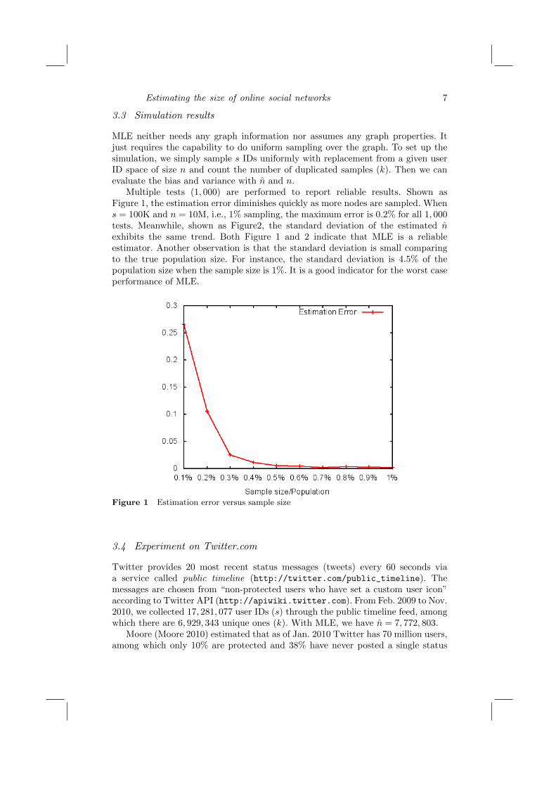
Multiple tests (1, 000) are performed to report reliable results. Shown asFigure 1, the estimation error diminishes quickly as more nodes are sampled. Whens = 100K and n = 10M, i.e., 1% sampling, the maximum error is 0.2% for all 1, 000tests. Meanwhile, shown as Figure2, the standard deviation of the estimated nexhibits the same trend. Both Figure 1 and 2 indicate that MLE is a reliableestimator. Another observation is that the standard deviation is small comparingto the true population size. For instance, the standard deviation is 4.5% of thepopulation size when the sample size is 1%. It is a good indicator for the worst caseperformance of MLE.

Figure 1 Estimation error versus sample size

3.4 Experiment on Twitter.com

Twitter provides 20 most recent status messages (tweets) every 60 seconds viaa service called public timeline (http://twitter.com/public_timeline). Themessages are chosen from “non-protected users who have set a custom user icon”according to Twitter API (http://apiwiki.twitter.com). From Feb. 2009 to Nov.2010, we collected 17, 281, 077 user IDs (s) through the public timeline feed, amongwhich there are 6, 929, 343 unique ones (k). With MLE, we have n = 7, 772, 803.

Moore (Moore 2010) estimated that as of Jan. 2010 Twitter has 70 million users,among which only 10% are protected and 38% have never posted a single status

8 S. Ye and S.F. Wu

Figure 2 Standard deviation versus sample size

message. Assuming these two numbers are independent, we have an estimation ofnon-protected users who have posted at least one status as 70× 90%× 62% = 37.8millions. There are several possible causes to explain the huge gap.

• These messages are sampled from a smaller population as described byTwitter API.

• The sample may not be uniform across all users. The public timeline serviceprovides random samples of messages instead of users. As some users postmore messages than others, this sample is likely skewed towards users withmore messages, which leads to underestimation of the size.

• The network grows during the sampling period. In the past 12 months, Twitterhas almost doubled its size (Moore 2010). It is hard to estimate a movingtarget.

• Twitter is a fast changing website. Its definition of public timeline may havechanged over the year. For example, as we have noticed, users with defaulticons are also shown in the public timeline.

4 Mark and recapture

Twitter’s public timeline data are a good candidate for mark and recapture, which iscommonly used in ecology to estimate the population size of a certain species (Seber1982). The basic idea is that if we perform two independent samplings on the samepopulation, the smaller the population is, the larger the overlap between these twosamples is likely to be. More specifically, m nodes are sampled uniformly fromthe population without replacement, and returned to the population after theyare marked. Then C nodes are sampled from the population without replacement.


Assuming R nodes in the second sample are marked (a.k.a. they are in the priorsampled list), the population size n can be estimated as

n =mC/R (10)

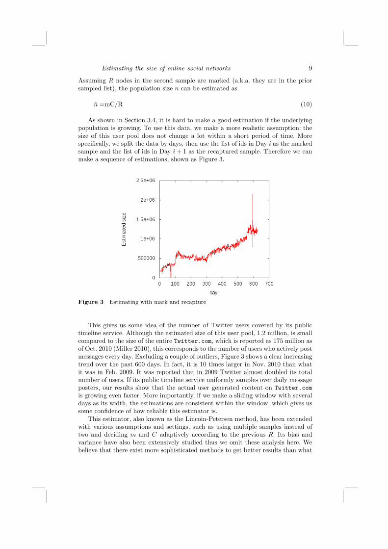
As shown in Section 3.4, it is hard to make a good estimation if the underlyingpopulation is growing. To use this data, we make a more realistic assumption: thesize of this user pool does not change a lot within a short period of time. Morespecifically, we split the data by days, then use the list of ids in Day i as the markedsample and the list of ids in Day i+ 1 as the recaptured sample. Therefore we canmake a sequence of estimations, shown as Figure 3.

Figure 3 Estimating with mark and recapture

This gives us some idea of the number of Twitter users covered by its publictimeline service. Although the estimated size of this user pool, 1.2 million, is smallcompared to the size of the entire Twitter.com, which is reported as 175 million asof Oct. 2010 (Miller 2010), this corresponds to the number of users who actively postmessages every day. Excluding a couple of outliers, Figure 3 shows a clear increasingtrend over the past 600 days. In fact, it is 10 times larger in Nov. 2010 than whatit was in Feb. 2009. It was reported that in 2009 Twitter almost doubled its totalnumber of users. If its public timeline service uniformly samples over daily messageposters, our results show that the actual user generated content on Twitter.com

is growing even faster. More importantly, if we make a sliding window with severaldays as its width, the estimations are consistent within the window, which gives ussome confidence of how reliable this estimator is.

This estimator, also known as the Lincoin-Petersen method, has been extendedwith various assumptions and settings, such as using multiple samples instead oftwo and deciding m and C adaptively according to the previous R. Its bias andvariance have also been extensively studied thus we omit these analysis here. Webelieve that there exist more sophisticated methods to get better results than what

10 S. Ye and S.F. Wu

we present in this section but the naive estimator already gives us some insights.As far as we know, this is the first estimation to the size of this population. As thisfeed is becoming widely used in many OSN studies, we encourage researchers toapply this estimation to their data.

5 Estimating with random walkers

When uniform sampling is unavailable or we can not get a lot of uniform samples,random walkers can be employed to estimate the size of the graph. This sectionintroduces an unbiased estimator (named as RW in this paper) proposed byMarchetti-Spaccamela (Marchetti-Spaccamela 1989) and evaluates this estimatorwith five real OSNs.

5.1 Estimating the size of a connected graph

Given a node v0, Marchetti-Spaccamela (Marchetti-Spaccamela 1989) estimates thenumber of nodes connecting to v0 with the following two-phase procedure.

1. Forward walking: Find a random acyclic path P starting from v0. Morespecifically, the random walker works as follows.

(a) Set P = φ and the current node to be v0.

(b) Assuming the current node is vi−1, uniformly select a neighbor vi.

(c) Terminate if vi does not have any outlinks (dead ends) or is a node therandom walker has previously visited (acyclic path), i.e., vi ∈ P.

(d) Add vi to P, i.e., P = {v0, v1, . . . , vi}.

(e) Return to Step (b).

When the random walker terminates, P consists of all the nodes the randomwalker has visited, except the terminating node.

2. Back tracing: For each node v ∈ P, we try to find an acyclic path betweenv0 and v in the reverse graph. Given a graph G(V,E), its reverse graph is

defined as G′(V,E′) where ∀−→ij ∈ E, we have−→ji ∈ E′ and vice versa. In the

reverse graph, a random walker generates acyclic paths starting from v aswhat we do in the forward walking phase. The random worker terminateswhen it reaches v0. If the random walker reaches a dead end or a previouslyseen node, it restarts from v. The only information we need to keep duringthis phase is the number of restarts it takes to reach v0, i.e., the number ofacyclic paths it generates.

To generalize this estimator in Section 6, we present its proof in detail, whichis initially provided by Marchetti-Spaccamela (Marchetti-Spaccamela 1989).

Given a random acyclic path P starting from v0, let Pv be the prefix of Pfinishing at v, i.e., Pv =< v0, v1, . . . , v >. Πout(Pv) denotes the product of the outdegrees of all the nodes in Pv except the last node v. Similarly Πin(Pv) denotes the


product of the in degrees of all the nodes in Pv except the first node v0. Finally, wedefine bP(v) = Πout(Pv)/Πin(Pv) and cP(v) to be the number of acyclic paths therandom walker generates in the back tracing phase. bv and cv are used as shorthandswhen there is no confusion of P given the context. We have the following theorem.

Theorem 3∑v∈P

bvcv is an unbiased estimator of the number of nodes connected to

v0.

Proof: To see this estimator is unbiased, we just need to show that its expectedvalue is the number of all the nodes connected to v0. The key to the proof is torewrite the expectation, a summation over all possible paths (P), as a summationover all the nodes connected to v0, i.e.,

E(∑v∈P

bvcv) =∑P

[(∑v∈P

bvcv)P(P)] (11)

=∑v

∑q∈Qv

bq(v)cq(v)P(q) (12)

=∑v

E(bq(v)cq(v)) (13)

where P(P) is the probability that P is chosen by the random walker, Qv is theset of all the acyclic paths from v0 to v, and P(q) is the probability for a randomwalker to walk through path q. To get the total number of nodes connected to v0,we just need to show that E(bq(v)cq(v)) = 1.

bq(v) is determined by the random path q. cq(v) is determined by the number ofrandom walks needed to backtrace v from v0. They are independent of each otherbecause the random walk is memoryless. Therefore we have

E(bq(v)cq(v)) = E(bq(v))E(cq(v)) (14)

The probability for the random walker to walk through a path q ∈ Qv is 1Πoutq

.Hence we have

E(bq(v)) =∑∀q∈Qv

bq(v)P(q) (15)

=∑∀q∈Qv

Πout(q)

Πin(q)P(q) (16)

=∑∀q∈Qv

1

Πin(q)(17)

Let Q′v be the set of all acyclic paths in the reverse graph G′ starting from v to v0.The probability for the random walker to walk through a path q ∈ Q′v is

∑∀q∈Q′

v

1

Πout(q)(18)


Notice that a path in G′ from v to v0 actually corresponds to a path in G fromv0 to v and the out degree of v in the G′ is the in degree of v in G. Therefore wehave ∑

∀q∈Qv

1

Πin(q)=∑∀q∈Q′

v

1

Πout(q)(19)

Combining (17) and (19), E(bq(v)) is the probability for the random walker to findan acyclic path from v to v0 in the reverse graph, which we denote as P(v → v0).

E(cq(v)) is the number of random walks needed to get a path in Q′v. As therandom walks are independent of each other, cq(v) follows a geometric distributionwith parameter P(v → v0) thus E(cq(v)) = 1

P(v→v0) .

Therefore we have E(bq(v))E(cq(v)) = 1. �

If G(V,E) is a connected graph, i.e., there exists a path between any two nodesin G, then the number of nodes connected to any node v is n− 1, where n is thesize of G. As a special case, for a node on an undirected graph, its in degree is equalto its out degree thus we have bv = v0/v, i.e., given a path P from node v0 to v, bvis solely decided by v0 and vi.

5.2 Experiments on real OSNs

To evaluate the RW estimator, we use four real OSN graphs collected by Mislove etal. (Mislove, Marcon, Gummadi, Druschel & Bhattacharjee 2007). Being publishedin 2007, these four graphs have been widely used in OSN studies. These fourOSNs are of different nature. Flickr (http://www.flickr.com) specializes inphoto sharing, YouTube focuses on video sharing, and LiveJournal (http://www.livejournal.com) and Orkut (http://www.orkut.com) are general socialwebsites. In addition, we crawled the entire Buzznet.com, another general OSNwebsite. Therefore the results reported here may apply to a variety of OSNs.

To avoid being trapped in small regions which are not connected to the majorityof the graph, we consider the largest connected components (LCC). Since thesegraphs are highly symmetrical and well connected, their LCCs cover a large portionof the original graphs, shown as Table 1. Orkut is supposed to be a bi-directedgraph but the data we got from Mislove et al. (Mislove et al. 2007) do containsome asymmetrical links. We suspect that it is caused by the crawling process.For example, node A is crawled before node B. By the time node A is crawled, Aand B are not connected yet. But when node B is crawled, A and B are alreadyconnected. As it takes a large amount of time to crawl huge graphs such as Orkut,such asymmetry is likely to be introduced.

Unless explicitly specified, for the rest of the paper we use LCCs instead of thewhole graphs. Table 2 summaries the basic properties of these five LCCs.

With LCCs, the number of nodes connected to any node is n− 1. From each ofthe five graphs we randomly select 2, 000 nodes as v0. The results given by the RWestimator are shown as Figure 4.

The small gaps between the true sizes and the estimated sizes suggest thatRW gives a good estimation to all these graphs. The large estimation error overLiveJournal indicates that more tests are needed for getting reliable results on thissocial graph.


Table 1 Largest connected components versus their original graphs

Graph Nodes in LCC Links in LCC

Buzznet 85.6% 72.6%

Flickr 79.4% 60.6%

LiveJournal 87.7% 72.7%

Orkut 99.9% 95.2%

YouTube 86.9% 78.3%

Table 2 Graphs used in our experiments

Graph Total Total Mean Clustering

(LCC) Nodes Links Degree Coefficient

Buzznet 423, 020 6, 616, 264 15.6 0.221

Flickr 1, 144, 940 13, 709, 764 12.0 0.136

LiveJournal 4, 033, 137 56, 296, 041 14.0 0.317

Orkut 2, 997, 166 212, 698, 418 71.0 0.170

YouTube 495, 957 3, 873, 496 7.8 0.110

Figure 4 Estimating the size of five OSNs with RW. Left bars represent the true sizesand right bars represent the estimated sizes.


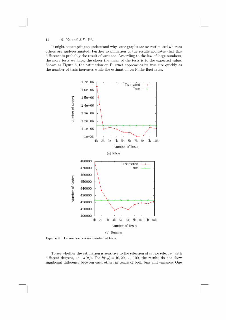
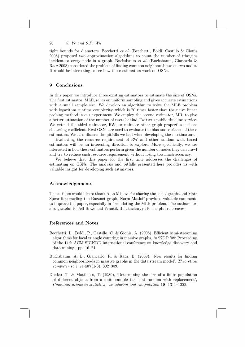
It might be tempting to understand why some graphs are overestimated whereasothers are underestimated. Further examination of the results indicates that thisdifference is probably the result of variance. According to the law of large numbers,the more tests we have, the closer the mean of the tests is to the expected value.Shown as Figure 5, the estimation on Buzznet approaches its true size quickly asthe number of tests increases while the estimation on Flickr fluctuates.

(a) Flickr

(b) Buzznet

Figure 5 Estimation versus number of tests

To see whether the estimation is sensitive to the selection of v0, we select v0 withdifferent degrees, i.e., k(v0). For k(v0) = 10, 20, . . . , 100, the results do not showsignificant difference between each other, in terms of both bias and variance. One


interesting observation is that the number of nodes crawled during the estimationbecomes smaller when high degree nodes are chosen for v0, shown as Figure 6. Tocompare the results on graphs with different size, the number of nodes crawled isnormalized by the number of nodes crawled when k(v0) = 10. For YouTube, thenumber of nodes which need to be crawled for k(v0) = 70 is about 50% smallerthan that for k(v0) = 10. Identifying the graph structure which causes this effect isan interesting direction for future work.

Figure 6 Number of nodes crawled (normalized by the number of nodes crawled whenk(v0) = 10) versus the degree of v0.

6 Generalizing the RW estimator

The proof of Theorem 3 actually provides a way to estimate other quantities besidesthe number of nodes in a graph.

Corollary 1 If ω(v) is not a random variable given node v,∑v∈P

ω(v)bvcv is an

unbiased estimator of∑vω(v).

Proof: Following Theorem 3 we have

E(∑∀v∈P

ω(v)bvcv) =∑v

E(ω(v)bvcv) (20)

=∑v

ω(v)E(bvcv) (21)

=∑v

ω(v) (22)


�

For example, if we set ω(v) to be the degree of v, then∑vω(v) is the total number

of links of the graph. In fact, we got similar results as Section 5.2 when applyingRW to estimate the number of links a graph has.

More generally, we have the following corollary:

Corollary 2 If ω(v) is a random variable independent of b(v) and c(v),∑∀v∈P

ω(v)bvcv is an unbiased estimator of∑vE(ω(v)).

Proof: Following Theorem 3 we have

E(∑∀v∈P

ω(v)bvcv) =∑v

E(ω(v)bvcv) (23)

=∑v

E(ω(v))E(bv)E(cv) (24)

=∑v

E(ω(v)) (25)

�

In other words, as long as the quantity of interest can be expressed as a randomvariable which is independent of b(v) and c(v), we can estimate it with thisapproach.

6.1 Estimating clustering coefficient

As an important metric for small world graphs, the clustering coefficient iscomputed and analyzed in many social network studies (Watts & Strogatz 1998).With Corollary 1, we may estimate the total clustering coefficient of a network(∑cc) if we set ω(v) to be the clustering coefficient of node v. Then an estimator

for the mean clustering coefficient of the network is given by∑cc

n(26)

This is a biased estimator because in general we have

E(cc) = E(

∑cc

n) 6= E(

∑cc)

E(n)(27)

If we know the size of the graph, we can have an unbiased estimator as follows.

E(cc) = E(

∑cc

n) =

E(∑cc)

n(28)

The difference is that n in (26) is a random variable thus needs to be estimatedwhereas the n in (28) is a known constant. The results given by these two estimators


(average of 1, 000 tests) are shown as Figure 7. To our surprise, the biased estimatoractually is not much worse than the unbiased one. On the YouTube graph, it evenoutperforms the unbiased estimator. A possible resolution is that the error of n

introduced by the random walker can be compensated by the error of∑cc in the

same run. Meanwhile, our analysis on the variance suggests that more tests for theunbiased estimator is needed to get closer to the true value.

Figure 7 Estimating the clustering coefficient of five OSNs with RW. Left barsrepresent the true value, middle bars represent the unbiased estimation givenby (28) and right bars represent the biased estimation given by (26).

7 Pitfalls

This section presents the pitfalls and challenges we encountered when developingestimators for OSNs. We believe that these discussions provide valuable insights forfuture work.

7.1 Combining MLE with MHRW

Gjoka et al. (Gjoka, Kurant, Butts & Markopoulou 2010) proposed an unbiasedsampling method, Metropolis-Hastings Random Walk (MHRW), to sample OSNs.We tried to combined MLE with MHRW. This approach would have twoadvantages.

• It does not rely on the OSN to provide uniform samples.

• It does not need to crawl lots of nodes.

This idea, however, does not work. Let Ψ = {v1, v2, . . . , v} be the set of nodescrawled by MHRW. MHRW generates a uniform sampling within Ψ, thereforecombining MLE with MHRW, we are only able to estimate the size of Ψ.


7.2 Large variance and expensive back tracing

There are two problems when we apply RW to large OSNs. First of all, the varianceis large. For example, among 30, 000 tests on Buzznet, only 24% of them haveestimation error within 50%. To get reliable estimations, we need the mean ofmultiple runs.

Secondly, during back tracing, RW may need lots of random walks before itreaches v0. For instance, in some cases, more than 90% of the graph are crawledbefore v0 is reached. On average, each test on the Buzznet graph crawls 254, 344nodes (60% of the entire graph). This number looks scary but it is skewed by asmall portion of random walkers which cover a majority of the graph.

It is possible to replace the back tracing with a breadth first search (BFS) andestimate a lower bound for the number of random walks needed to reach v0, butdue to the small world property of OSNs, BFS is likely to cover a large portion ofthe graph as well, as shown by Ye et al. (Ye, Lang & Wu 2010).

To finish the back tracing quickly, parallel random walkers can be used whilecareful coordination needs to be implemented. To avoid duplicated crawlings, weneed to cache visited nodes across multiple random walkers. Once a random walkerreaches v0, all the random walkers need to be stopped (to save the crawling costs)and the random walkers starting after the one which reaches v0 should be discarded(otherwise the number of random walks needed to reach v0 will be overestimated).

7.3 Poor lower and upper bounds for RW

Marchetti-Spaccamela (Marchetti-Spaccamela 1989) proposed an estimator for thelower bound of RW, which performs up to k random walks in the back tracingphase. If after k random walks, v0 is still not reached, k is returned as the minimumnumber of random walks needed to reach v0. Without prior knowledge of the graphsize, however, it is nontrivial to set a proper k: Large ks do not serve the purposeof accelerating the back tracing whereas small ks produce poor lower bounds. Inour experiments, with k = 1M, the lower bounds given by this estimator are stillpoor for large graphs such as LiveJournal and Orkut.

An upper bound is also proposed in (Marchetti-Spaccamela 1989) which simplyassumes that G is a tree instead of a graph. This estimator, however, greatlyoverestimates the size when G is large. On our graphs the upper bound estimatoroverestimates by several magnitudes.

7.4 Expensive computation costs in simulations

Simulations on large graphs such as OSNs are computationally expensive. In ourtests, we used a cluster of 36 PCs with two AMD Opteron 2.6GHz CPU/4GBmemory per node. It took us a month to finish various tests presented here. Toimprove the performance, we have the following optimizations.

• Tight data structures: An adjacency list (array) is used to represent theneighbors of each node. A large array is used to keep pointers to these liststherefore random access to any list is simple and fast. Initially we used theIDs coming with the datasets, which are not continuous especially when we


deal with LCCs. To make the array as small as possible, we reassign the IDsfor the nodes in LCCs such that they are continuous.

• Accelerating frequently executed routines: As a lot of similar operations areperformed multiple times, making such components faster greatly reduces thesimulation time.

For example, we need to set/check whether a node has been visited whentrying to find an acyclic path. This was initially implemented with a set inthe C++ Standard Template Library (STL). Set is implemented with treesbut we actually do not need to keep the order of the items. Then we changedto unordered set, which is a hash table. Being still not satisfied with itsperformance, we finally replaced it with a bit field where each bit correspondsto a node, then the check is done by simply examining whether the bit is setor not.

Another example is that we sort the IDs within each adjacency list such thatwhen computing clustering coefficients, a binary search can be applied tocheck if the list has a certain node.

• Improving data locality : The random walker incurs a lot of cache misses, whichbecome the main bottleneck of our simulation. More specifically, after therandom walker visits a node v, it needs to check v’s neighbors, say Nv, thenit moves to u ∈ Nv and checks u’s neighbors, say Nu. If the two adjacencylists corresponding to Nv and Nu are far away from each other, a cache missis likely to happen. To alleviate this problem, we malloc a large continuousmemory pool for the adjacency lists and rearrange them to keep adjacencylists of neighbors close to each other in the memory layout. Although therandom walker makes it impossible to predict the precise access order, ourexperimental results show that this simple optimization reduces a lot of cachemisses.

With all the optimizations applied, the simulation runs 10− 20 times faster.

8 Related work

The coupon collector’s problem (Feller 1957) asks the following question: Givenn coupons, from which coupons are randomly sampled with replacement, what isthe probability that s sample trials are needed to collect all n coupons? In ourMLE problem, n is the quantity of interest while in coupon collector’s problem, nis known and the number of unique coupons which have been collected (k) is thequantity of interest.

Knuth (Knuth 1975) proposed an unbiased estimator to estimate the size of atree with random walkers. Pitt (Pitt 1987) extended this estimator to estimate thesize of directed acyclic graphs (DAGs). These two pieces of work inspire the RWestimator, which we have discussed in detail in Section 5.1.

Besides estimating the size of graphs, there are studies on estimating other graphproperties but few of them focuses on OSNs. Tsonis et al. (Tsonis, Swanson &Wang 2008) proposed an estimator for clustering coefficient in scale free networks.Magnien et al. (Magnien, Latapy & Habib 2009) developed a fast algorithm to find


tight bounds for diameters. Becchetti et al. (Becchetti, Boldi, Castillo & Gionis2008) proposed two approximation algorithms to count the number of trianglesincident to every node in a graph. Buchsbaum et al. (Buchsbaum, Giancarlo &Racz 2008) considered the problem of finding common neighbors between two nodes.It would be interesting to see how these estimators work on OSNs.

9 Conclusions

In this paper we introduce three existing estimators to estimate the size of OSNs.The first estimator, MLE, relies on uniform sampling and gives accurate estimationswith a small sample size. We develop an algorithm to solve the MLE problemwith logarithm runtime complexity, which is 70 times faster than the naive linearprobing method in our experiment. We employ the second estimator, MR, to givea better estimation of the number of users behind Twitter’s public timeline service.We extend the third estimator, RW, to estimate other graph properties such asclustering coefficient. Real OSNs are used to evaluate the bias and variance of theseestimators. We also discuss the pitfalls we had when developing these estimators.

Evaluating the resource requirement of RW and other random walk basedestimators will be an interesting direction to explore. More specifically, we areinterested in how these estimators perform given the number of nodes they can crawland try to reduce such resource requirement without losing too much accuracy.

We believe that this paper for the first time addresses the challenges ofestimating on OSNs. The analysis and pitfalls presented here provides us withvaluable insight for developing such estimators.

Acknowledgements

The authors would like to thank Alan Mislove for sharing the social graphs and MattSpear for crawling the Buzznet graph. Norm Matloff provided valuable commentsto improve the paper, especially in formulating the MLE problem. The authors arealso grateful to Jeff Rowe and Prantik Bhattacharyya for helpful references.

References and Notes

Becchetti, L., Boldi, P., Castillo, C. & Gionis, A. (2008), Efficient semi-streamingalgorithms for local triangle counting in massive graphs, in ‘KDD ’08: Proceedingof the 14th ACM SIGKDD international conference on knowledge discovery anddata mining’, pp. 16–24.

Buchsbaum, A. L., Giancarlo, R. & Racz, B. (2008), ‘New results for findingcommon neighborhoods in massive graphs in the data stream model’, Theoreticalcomputer science 407(1-3), 302–309.

Dhakar, T. & Mattheiss, T. (1989), ‘Determining the size of a finite populationof different objects from a finite sample taken at random with replacement’,Communications in statistics - simulation and computation 18, 1311–1323.


Driml, M. & Ullrich, M. (1967), ‘Maximum likelihood estimate of the number oftypes’, Acta Technica CSAV pp. 300–303.

Feller, W. (1957), Introduction to probability and its applications, Vol. 1, secondedn, John Wiley.

Finkelstein, M., Tucker, H. G. & Veeh, J. A. (1998), ‘Confidence intervals for thenumber of unseen types’, Statistics and probability letters 37(4), 423–430.

Gjoka, M., Kurant, M., Butts, C. T. & Markopoulou, A. (2010), Walking inFacebook: A case study of unbiased sampling of OSNs, in ‘Proceedings of the2010 IEEE Infocom conference’, pp. 1–9.

Gross, R., Acquisti, A. & Heinz, III, H. J. (2005), Information revelation and privacyin online social networks, in ‘WPES ’05: Proceedings of the 2005 ACM workshopon privacy in the electronic society’, pp. 71–80.

Knuth, D. E. (1975), ‘Estimating the efficiency of backtrack programs’, Mathematicsof computation 29(129), 121–136.

Magnien, C., Latapy, M. & Habib, M. (2009), ‘Fast computation of empirically tightbounds for the diameter of massive graphs’, Journals of experimental algorithmics13, 1.10–1.9.

Marchetti-Spaccamela, A. (1989), ‘On the estimate of the size of a directed graph’,Graph-theoretic concepts in computer science 344, 317–326.

Miller, C. C. (2010), ‘Why twitters c.e.o. demoted himself’. http://www.nytimes.com/2010/10/31/technology/31ev.html.

Mislove, A., Marcon, M., Gummadi, K. P., Druschel, P. & Bhattacharjee, B. (2007),Measurement and analysis of online social networks, in ‘IMC’07: Proceedings ofthe 7th ACM SIGCOMM conference on Internet measurement’, pp. 29–42.

Moore, R. J. (2010), ‘New data on Twitter’s users andengagement’. http://themetricsystem.rjmetrics.com/2010/01/26/

new-data-on-twitters-users-and-engagement/.

Pitt, L. (1987), ‘A note on extending Knuth’s tree estimator to directed acyclicgraphs’, Information processing letters 24(3), 203–206.

Seber, G. (1982), The Estimation of Animal Abundance, The Blackburn Press.

Tsonis, A., Swanson, K. & Wang, G. (2008), ‘Estimating the clustering coefficientin scale-free networks on lattices with local spatial correlation structure.’, PhysicaA: Statistical mechanics and its applications 387, 5287–5294.

Watts, D. J. & Strogatz, S. H. (1998), ‘Collective dynamics of ’small-world’networks’, Nature 393, 440–442.

Ye, S., Lang, J. & Wu, F. (2010), Crawling online social graphs, in ‘APWeb ’08:Proceeding of the 2010 Asia Pacific Web conference’, pp. 236–242.

Estimating the Size of Online Social Networks Shaozhi Ye* S. Felix Wu

Documents

Transcript of Estimating the Size of Online Social Networks Shaozhi Ye* S. Felix Wu