Estimating the Effects of the Terminal Area Productivity ...
106
NASA Contractor Report 201682 Estimating the Effects of the Terminal Area Productivity Program David A. Lee, Peter F. Kostiuk, Robert V. Hemm, Earl R. Wingrove III, and Gerald Shapiro Logistics Management Institute, McLean, Virginia Contract NAS2-14361 April 1997 National Aeronautics and Space Administration Langley Research Center Hampton, Virginia 23681-0001
Transcript of Estimating the Effects of the Terminal Area Productivity ...

NASA Contractor Report 201682
Estimating the Effects of the Terminal Area Productivity Program
David A. Lee, Peter F. Kostiuk, Robert V. Hemm, Earl R. Wingrove III, and Gerald ShapiroLogistics Management Institute, McLean, Virginia
Contract NAS2-14361
April 1997
National Aeronautics andSpace AdministrationLangley Research CenterHampton, Virginia 23681-0001

iii
Estimating The Effects Of The Terminal AreaProductivity Program
SUMMARY
We describe the methods and results of an analysis of the technical and economicbenefits of the systems to be developed in the NASA Terminal Area Productivity(TAP) program. We developed a methodology for analyzing the technical and eco-nomic benefits of the TAP systems. To estimate airport capacity, the methodologyuses inputs from airport-specific data on hourly weather, hourly operations counts,operating configurations, and mixes of transport aircraft types. The capacity modeluses parameters that reflect the potential impacts of the TAP systems. The analyticapproach takes the capacity estimates, calculates aircraft delays through a queuingmodel, and calculates the cost savings to airlines from reduced delays. The modelanalyzes the impact of advanced aviation technologies and changes in operating pro-cedures on terminal area operations.
We establish preliminary estimates of the benefits of the TAP systems. As the TAPsystems become better defined, more accurate and detailed analyses of the benefits ofimplementing these systems will be possible. Outputs from the analysis are prelimi-nary estimates of the benefits of the TAP systems. Technical benefits include reduc-tions in both means and variances of aircraft-minutes of delay; the latter reductionsare important to airlines interested in schedule integrity. We estimate savings in air-line operating costs from reduced delays.
The airport capacity estimates rest on three model pillars, two operational and oneeconomic. For each of the two airports analyzed, these are a model of the airport ca-pacity as a function of weather conditions, with parameters that can be adjusted to re-flect impacts of the TAP technologies; a model of operations demand as a function oftime; and a model of airline operating costs.
We applied the analytic method to Boston’s Logan International (BOS) and Detroit’sWayne County (DTW) airports. Tables 1 through 4 summarize the key aircraft delayresults. For each selection of TAP systems, airport capacity and the resulting delayswere calculated and the airline cost savings computed. Tables 1 and 2 show theestimated annual aircraft delays for BOS and DTW for selected years, with andwithout the TAP systems. The estimates indicate a sharp increase in delays throughthe year 2015, as demand grows steadily and capacity increases are limited. There aresizable delay reductions from the TAP systems, as much as 50 percent from all TAP

iv
systems operating at BOS in 2015. Table 3 shows the estimated cost of the baselinedelays, based on estimates of aircraft operating costs and the mix of aircraft nowflying into those two airports. An upper and lower bound on delay costs is providedto account for the uncertainty in where the delay is incurred (such as on the ground orwhile airborne). To quantify the impacts of some of the individual TAP systems, wedefined three combinations of TAP systems. These are labeled TAP 1, TAP 2, andTAP 3.
TAP 1. The first TAP increment, Reduced Spacing Operations (RSO) includes theAircraft Vortex Spacing System (AVOSS) with wake vortex sensors. We expect theseelements to reduce the arrival separations currently maintained to avoid wake vortexthreats.
TAP 2. The second TAP increment, Low Visibility Landing and Surface Operations(LVLASO) includes GPS precision landing capability plus cockpit taxi maps and sen-sor systems necessary to reduce arrival runway occupancy time during instrumentmeteorological conditions by 20 percent.
TAP 3. The third TAP increment, Advanced Traffic Management Center (ATM) in-cludes integrated CTAS/FMS (Center TRACON Automation System/Flight Man-agement System). Integration assumes two-way CTAS/FMS data linking. In the TAP3 increment, CTAS would be operating “closed loop” with the current flight plans ofindividual aircraft. Moreover, the FMS capability provides high confidence that theplans will be carried out as described. Flight plan revisions will be communicatedboth ways in real time. The parametric result will be reduced uncertainty about air-craft status and intent that permits reducing Instrument Flight Rule (IFR) separationsto near Visual Flight Rule (VFR) distances.
Table 1. Annual Aircraft Arrival Delay at BOS (Millions of Minutes)
TechnologyState
1993 2005 2015
Current 5.5 6.8 12.2
TAP 1 – 5.9 10.8
TAP 2 – 4.8 8.9
TAP 3 – 2.1 4.2

Estimating the Effects of the Terminal Area Productivity Program
v
Table 2. Annual Aircraft Arrival Delay at DTW (Millions of Minutes)
TechnologyState
1995 2005 2015
Current 1.1 1.6 2.8
TAP 1 – 1.5 2.6
TAP 2 – 1.4 2.0
TAP 3 – 1.1 1.4
Table 3. Annual Aircraft Delay Costs (1993 $ Millions)
Airport 1993 ($) 2005 ($) 2015 ($)
Boston, upper bound 161 197 354
Boston, lower bound 90 110 198
Detroit, upper bound 37 55 95
Detroit, lower bound 21 31 53
The analysis leads us to conclude that implementing the TAP technologies will leadto substantial savings at BOS and DTW, although the amounts differ. Moreover, thereare substantial benefits from each of the TAP technologies, as shown in Table 4.
Table 4. Present Value of TAP Benefits (1993 $ millions)
AirportTAP increment
1 ($)TAP increment
2 ($)TAP increment
3 ($) Total ($)
Boston, upperbound
165 236 542 937
Boston, lowerbound
92 129 302 523
Detroit, upperbound
24 62 70 157
Detroit, lowerbound
14 35 39 88
One conclusion of the study is that, for values of miles-in-trail separations and runwayoccupancy times consistent with the best data we found, both must be reduced if the

vi
benefits of either are to be realized. Benefits of reduced miles-in-trail separations canbe enjoyed only so long as runway occupancy times do not become the binding con-straint, and similarly there is little benefit from reduced runway occupancy time ifseparations are not reduced. For this reason it is difficult to separate the benefits ofRSO’s reduced separations from the benefits of LVLASO’s reduced runway occu-pancy times.
We also find that additional data collection would benefit our analysis.

vii
Contents
Estimating The Effects Of The Terminal Area Productivity Program ...............iii
SUMMARY ........................................................................................................................... iii
Chapter 1 Overview...........................................................................................1-1
TERMINAL AREA PRODUCTIVITY RESEARCH PROGRAM....................................................1-1
Objectives of this Study .............................................................................................1-4
Chapter 2 Characteristics of Weather and Delays at BOS and DTW...............2-1
DEFINITIONS OF OPERATING CATEGORIES AT THE STUDY AIRPORTS.................................2-1
DELAY AND WEATHER DATA ............................................................................................2-2
Delays and Weather at Boston...................................................................................2-3
Delays and Weather at Detroit...................................................................................2-9
SUMMARY AND CONCLUSIONS ON OBSERVED DELAYS...................................................2-13
Chapter 3 Modeling Airport Capacity..............................................................3-1
OVERVIEW ........................................................................................................................3-1
PARAMETRIC CAPACITY ANALYSES AND SIMULATIONS ....................................................3-2
Chapter 4 Estimating Delay..............................................................................4-1
QUEUING MODELS OF AIRPORT OPERATIONS....................................................................4-1
THE FLUID APPROXIMATION MODEL.................................................................................4-2
Modeling Arrival and Departure Demand..................................................................4-3
Chapter 5 Estimating the Impacts of TAP Technologies on Capacity andDelay at BOS and DTW..........................................................................5-1
CAPACITY MODEL PARAMETERS AND THEIR CORRELATION WITH TAP TECHNOLOGIES..5-1
THE FIVE TECHNOLOGY STATES MODELED ......................................................................5-2
Model Parameters and Their Relations to the Technology States..............................5-3

viii
Runway Configuration...............................................................................................5-4
TIME SERIES OF WEATHER AT BOS.................................................................................5-14
TIME SERIES OF WEATHER AT DTW ...............................................................................5-15
FUTURE DEMAND AT BOS ..............................................................................................5-15
Discussion ................................................................................................................5-16
RESULTS AT BOS FOR 2015 ............................................................................................5-16
Weather Data............................................................................................................5-16
Demand Data............................................................................................................5-17
MODEL RESULTS AT DTW ..............................................................................................5-17
Weather Data............................................................................................................5-17
Demand Data............................................................................................................5-18
Discussion ................................................................................................................5-18
Chapter 6 Converting Estimated Delays Into Air Carrier Costs.......................6-1
SOME DEFINITIONS............................................................................................................6-1
FORM 41 DATA .................................................................................................................6-1
ESTIMATED SYSTEM-WIDE DELAY COSTS PER BLOCK MINUTE ........................................6-2
OPERATIONS AT BOSTON’S LOGAN INTERNATIONAL AIRPORT AND DETROIT’S WAYNE
COUNTY AIRPORT.................................................................................................6-3
ARRIVAL DELAY COSTS AT BOSTON’S LOGAN INTERNATIONAL AIRPORT AND
DETROIT’S WAYNE COUNTY AIRPORT..................................................................6-4
POTENTIAL SAVINGS FROM TAP TECHNOLOGIES..............................................................6-5
ADDITIONAL DATA NEEDED..............................................................................................6-7
CONCLUSIONS...................................................................................................................6-8
Appendix A Statistics of Interarrival and Interdeparture Times and the LMIRunway Capacity Model.........................................................................A-1
OPERATING CASES MODELED..........................................................................................A-1
Arrivals only..............................................................................................................A-3
Statistics of Multiple Operations...............................................................................A-8
Departures ...............................................................................................................A-13

Contents
ix
PASCAL CODE FOR THE LMI RUNWAY CAPACITY MODEL.............................................A-16
FIGURES
Figure 1-1. Overview of the Analysis Method.......................................................................1-6
Figure 2-1. Average Delays by Operating Conditions, BOS Arrivals in 1993......................2-4
Figure 2-2. Delays by Phase of Flight and Time of Day, BOS VFR1 arrivals in 1993.........2-5
Figure 2-3. Annual Operating Conditions at BOS.................................................................2-6
Figure 2-4. Boston Weather and Operating Mode.................................................................2-7
Figure 2-5. Boston Fog by Hour.............................................................................................2-8
Figure 2-6. Boston Haze by Hour...........................................................................................2-8
Figure 2-7. Annual Operating Conditions at DTW................................................................2-9
Figure 2-8. Detroit Weather and Operating Mode...............................................................2-10
Figure 2-9. Detroit Fog by Hour...........................................................................................2-10
Figure 2-10. Detroit Haze by Hour.......................................................................................2-11
Figure 2-11. Average Delays by Operating Conditions, DTW Arrivals in 1993.................2-12
Figure 2-12. Delays by Phase of Flight and Time of Day DTW VFR1 Arrivals in 1993...2-12
Figure 3-1. Example Airport Capacity...................................................................................3-1
Figure 3-3. Runway Capacity Model Output.........................................................................3-5
Figure 3-4. Detroit Figure from ASC Plan.............................................................................3-7
Figure 3-5. BOS Airport Layout from ASC Plan...................................................................3-8
Figure 4-1. Exact Mean Queue and Fluid Approximation.....................................................4-3
Figure A-1. Time Phase for Arrivals when Follower Velocity > Leader Velocity...............A-2
Figure A-2. Time Phase of Arrivals when Follower Velocity < Leader Velocity.................A-6
Figure A-3. Time Phase of Arrivals with Intervening Departure..........................................A-8
Figure A-4. Interarrival Time (Distribution).........................................................................A-9
Figure A-5. Time Phase of Departures................................................................................A-13

x
TABLES
Table 1. Annual Aircraft Arrival Delay at BOS (Millions of Minutes)................................... iv
Table 2. Annual Aircraft Arrival Delay at DTW (Millions of Minutes)................................... v
Table 3. Annual Aircraft Delay Costs (1993 $ Millions).......................................................... v
Table 4. Present Value of TAP Benefits (1993 $ millions)....................................................... v
Table 1-1. Reduced Spacing Operations................................................................................1-2
Table 1-2. Low Visibility Landing and Surface Operations (LVLASO)...............................1-3
Table 1-3. Air Traffic Management.......................................................................................1-3
Table 2-1. Ceiling and Visibility for Operating Conditions at BOS and DTW.....................2-2
Table 2-2. Total Delays at BOS in 1993 (in Thousands of Minutes).....................................2-5
Table 2-3. Distribution of Arrival Delays at BOS in 1993 (by Meteorological Conditions).2-6
Table 3-1. Capacity Model Parameters—Comparison...........................................................3-4
Table 5-1. Runway Capacity Model Parameters; Comparison..............................................5-3
Table 5-2. Aircraft Weight Categories...................................................................................5-4
Table 5-3. Current Reference Interarrival Separations (in Nautical Miles)...........................5-7
Table 5-4. TAP 1 Interarrival Separations (in Nautical Miles).............................................5-8
Table 5-5. TAP 3 Interarrival Separations (in Nautical Miles)..............................................5-8
Table 5-6. Interarrival Time Uncertainty Parameters...........................................................5-10
Table 5-7. Current Reference Departure Separations in Seconds........................................5-12
Table 5-8. Comparison of LMI and FAA Capacity Model Results for a Single Runway atBOS................................................................................................................................5-14
Table 5-9. Annual Aircraft Arrival Delay at BOS (Millions of Minutes)............................5-17
Table 5-10. Aircraft Delay at DTW for TAP Implementations (in Millions of Minutes)....5-18
Table 6-1. Passenger Airline Operating Statistics..................................................................6-2
Table 6-2. System-wide Delay Costs by Type of Aircraft.....................................................6-3
Table 6-3. Operations at Boston, Logan Airport....................................................................6-4
Table 6-4. Operations at Detroit, Wayne County Airport......................................................6-4
Table 6-5. Airport-Specific Cost per Minute of Arrival Delay..............................................6-5

Contents
xi
Table 6-6. Aircraft Minutes of Arrival Delay........................................................................6-5
Table 6-7. Airline Arrival Delay Costs ($ Millions).............................................................6-6
Table 6-8. Present Value of Arrival Delay Costs Avoided ($ Millions)...............................6-6
Table A-1. Key Airport Modeling Parameters......................................................................A-1

1-1
Chapter 1
Overview
This section provides background information on the NASA Terminal Area Produc-tivity (TAP) research program. It sets out the objectives of the study, and briefly de-scribes the approach developed to meet them.
TERMINAL AREA PRODUCTIVITY RESEARCH PROGRAM
The goal of the TAP research program is to safely achieve visible flight rule (VFR)capacity in instrument flight rule (IFR) conditions. In cooperation with the FederalAviation Administration (FAA), NASA’s approach is to develop and demonstrateairborne and ground technology and procedures to safely reduce aircraft spacing interminal areas, enhance air traffic management and reduce controller workload, im-prove low-visibility landing and surface operations, and integrate aircraft and air traf-fic systems. By the end of the decade, integrated ground and airborne technology willsafely reduce spacing inefficiencies associated with single runway operations and therequired spacing for independent, multiple-runway operations conducted under in-strument flight rules.
The NASA TAP program consists of four major program elements: Air Traffic Man-agement (ATM), Reduced Spacing Operations (RSO), Low Visibility Landing andSurface Operations (LVLASO), and Aircraft/ATC System Integration. The ATMelement builds on the Center TRACON Automation System (CTAS) Program cur-rently being supported under the NASA base program and the FAA Terminal AirTraffic Control Automation (TATCA) Program. The RSO element focuses onbuilding systems to reduce current aircraft spacing standards in terminal areas.LVLASO concentrates on developing technologies to cut delays on the ground duringperiods of poor visibility.
The fourth element of TAP, Aircraft/ATC Systems Integration, focuses on ensuringthat the various systems developed under the other elements fit consistently into theoverall system. The goals of this element are threefold: (1) Ensure coordination andintegration between airborne and ground-side elements; (2) provide flight facilitysupport; and (3) develop and maintain the systems focus with technology impact andcost-benefit analysis. This study was performed as part of the Aircraft-ATC SystemsIntegration element.

1-2
Each of the three research elements contains several projects. The most authoritativeinformation about project products, milestones, and budgets is found in the Level 3element program plans. NASA briefing material and interviews with NASA person-nel augment the information from the Level 3 plans.
Tables 1-1 through 1-3 list the three TAP elements and projects along with supple-mental information on technology content. The firmness of the projects varies con-siderably. Some projects such as lidar and radar vortex sensors are well-defined,while others such as those in LVLASO, RSO information for lateral spacing, andRSO CTAS/FMS integration are periodically revised, removed, and reinstated.
Table 1-1. Reduced Spacing Operations
Technology Program Area Technology Products
Wake Vortex Systems • Aircraft Vortex Spacing System (AVOSS)
• Lidar Wake Vortex Sensor
• Radar Wake Vortex Sensor
• Demonstrated AVOSS prototype includingintegration of wake vortex prediction andsensing, weather, and aircraft information
Center TRACON Automation Sys-tem Compatible Flight ManagementSystem Development (CTAS Com-patible FMS)
• Increasingly comprehensive simulations ofintegrated CTAS/FMS operations
• Flight tested full CTAS coordinated with FMS
Airborne Information for LateralSpacing (AILS)
• Techniques to improve navigation precision onclosely spaced parallel approaches
• Conflict alerting, detection, and appropriatedisplays
• Air/ground information technologies
• Airborne flight test of the Improved NavigationPerformance (INP) subsystem

Overview
1-3
Table 1-2. Low Visibility Landing and Surface Operations (LVLASO)
Technology Program Area Technology Products
Reduced Runway Occupancy Time • Roll Out & Turn Off system (ROTO)
• Enhanced ROTO/DGPS-based landing sys-tem
• ROTO & landing system requirements
Efficient and Safe Surface andTower Guidance
• Taxi Navigation and Situation Awarenesssystem (T-NASA)
• 3-D auditory display for blunder detection andavoidance
• Recommended crew procedures and air trafficmanagement interface
Terminal Area Systems Integration/Evaluation
• Required navigation performance (RNP) forROTO& surface operations
• Dynamic Runway Occupancy MeasurementSystem (DROMS)
• Integration of Surface Management Advi-sor/Guidance & Control/Information presenta-tion
Table 1-3. Air Traffic Management
Technology Program Area Technology Products
Center TRACON AutomationSystem/Flight
Management System Development(CTAS/FMS Integration)
• Data exchange, fusion, and sharing tech-niques
• FMS operations in the ARTCC for descents
• FMS operations in the Terminal Radar Ap-proach Control area
• Field test of full CTAS/FMS scenario
Dynamic Routing • CTAS automation tools for efficiently re-routing aircraft
Precision Approach to CloselySpaces Parallel Runways (PACSPR)
• CTAS Final Approach Spacing Tool (FAST)support for offset approaches
Dynamic Spacing • CTAS/FAST integrated with AVOSS and
DROM

1-4
At completion of TAP research and development in 2000, the technology require-ments will be established by analysis and testing (validation). Hardware and softwarefeasibility will be demonstrated by integrated tests (demonstration). The next phaseof TAP development varies with the technology. Wake vortex sensors and otherR&D hardware will require engineering and manufacturing development, probably bythe FAA, while software products like CTAS upgrades may need no further develop-ment. (Some modifications of software will be required to meet FAA reliability andhardening standards.) Suites of commercial off-the-shelf hardware, like flight man-agement systems and data links, may need no further development, but will requirepurchase or upgrading by individual airlines. TAP product categories consist of:
◆ algorithms and software that can be installed in existing FAA and aircraftsystems,
◆ validated specifications supported by feasibility demonstrations for hardwareto be further developed and purchased by the FAA, and
◆ specifications and recommendations for new or modified commercial off-the-shelf avionics to be purchased by the FAA and aircraft owners.
Objectives of this Study
This study aims to provide the analysis tools needed to estimate the potential impactand benefits of the systems under development in the NASA TAP program. The ba-sic approach to the analysis is straightforward:
1. Quantitatively confirm that weather is the primary cause of reduced ca-pacity and delay at the study airports.
2. Quantify the major weather patterns at the study airports.
3. Identify those weather conditions and airports at which the TAP systemsmay provide benefits.
4. Develop the analysis method and estimate the potential impacts of TAP onoperations at the first two airports of interest.
This report summarizes the results of this analysis and describes the method used toquantify the benefits of the TAP systems. The method can be used to analyze otherterminal area issues, such as changes in regulations or alternative operating proce-dures. We applied the method to analyses of Boston’s Logan International Airport(BOS) and Detroit’s Wayne County International Airport (DTW).

Overview
1-5
The TAP systems are designed to enable airports to operate in poor weather with thesame efficiency that they operate in good weather. Poor weather limitations derivefrom the need for air traffic controllers to operate under instrument flight rules main-taining constant positive control of aircraft separations as opposed to sharing the re-sponsibility with the pilots as is done in good weather under visual flight rules. Thequality of aircraft data available to controllers and limits on human ability to managemultiple aircraft safely in poor weather result in conservative aircraft spacing andlower landing and takeoff rates. The TAP systems provide improved data and auto-mation aids to help the controllers and the pilots operate at higher rates in poorweather. Consequently, this report begins with an extensive discussion of howweather affects airport operations and specifically arrival delays.
This study concentrated on arrival delays for two reasons: First, for many days onwhich study airports have significant arrival delays, the models indicate that departurecapacity is not reduced as seriously as arrival capacity. Second, while it seems reason-able in this initial study to assume that the time-phasing of arrival demand generallyfollows the standard pattern for a given day, that assumption may not be reasonablefor departure demand. Significant arrival delays seem certain to alter the time phas-ing of departure demand; on bad days, most arrivals will experience significant de-lays. Estimating departure delays even at a single airport, requires a model of theinteraction between delayed arrivals and subsequent departures. A multi-airport net-work analysis is required to estimate properly the propagation of delays throughout anaircraft itinerary.
Also, we believe that airline choices affect data on departure delays. For example,there is some anecdotal evidence that airplanes often push back from the gate eventhough the crews know they will not be able to take off immediately, so that FAAground holds will not be charged to the airlines. Unfortunately, this practice alsocauses the ground hold to be recorded as taxi-out delay. Concentrating on arrival de-lays allows a cleaner, more reliable link between TAP technologies and benefits. Theimpact of this decision is some conservatism in the benefit calculations: None of theTAP systems will increase departure delays; most should reduce them.
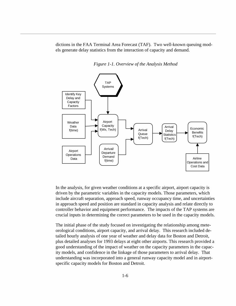
Figure 1-1 summarizes the approach employed in this study. The analysis focuses onaircraft-minutes of arrival delay in the terminal area as the principal performancemeasure. Estimating delay requires calculating airport capacity, airport demand, andidentifying relationships among capacity, demand, and delay. This study uses both astandard model and a newly developed model to estimate airport capacity as a func-tion of weather and aircraft and air traffic control parameters. Airport tower recordsprovide the required measures of demand. Future demand is forecasted with the pre-
1-6
dictions in the FAA Terminal Area Forecast (TAF). Two well-known queuing mod-els generate delay statistics from the interaction of capacity and demand.
In the analysis, for given weather conditions at a specific airport, airport capacity isdriven by the parametric variables in the capacity models. Those parameters, whichinclude aircraft separation, approach speed, runway occupancy time, and uncertaintiesin approach speed and position are standard in capacity analysis and relate directly tocontroller behavior and equipment performance. The impacts of the TAP systems arecrucial inputs in determining the correct parameters to be used in the capacity models.
The initial phase of the study focused on investigating the relationship among mete-orological conditions, airport capacity, and arrival delay. This research included de-tailed hourly analysis of one year of weather and delay data for Boston and Detroit,plus detailed analyses for 1993 delays at eight other airports. This research provided agood understanding of the impact of weather on the capacity parameters in the capac-ity models, and confidence in the linkage of those parameters to arrival delay. Thatunderstanding was incorporated into a general runway capacity model and in airport-specific capacity models for Boston and Detroit.
Figure 1-1. Overview of the Analysis Method
Weather Data f(time)
Identify Key Delay and Capactiy Factors
f(Wx)
Airport Operations
Data
TAP Systems
Arrival Delay
Statistics f(Tech)
Airport Capacity
f(Wx, Tech)
Arrival/ Departure Demand
f(time)
Economic Benefits f(Tech)
Airline Operations and
Cost Data
Arrival Queue f(Tech)

Overview
1-7
The NASA TAP program documentation identifies the products of the technologyprojects. We worked with NASA to develop the relationships between those productsand airport capacity parameters. Three ensembles of products for deployment in threeTAP implementations were analyzed in order to estimate the individual effects of theTAP systems. Capacity model parameter values were estimated for a year 2005baseline and for each TAP implementation. The three TAP implementations (TAP 1,2, and 3) are cumulative in that TAP 2 adds to TAP 1 and TAP 3 adds to TAP 2.
Two steps were required to link delay reductions to changes in airline operating costs.First, we identified the elements of airline operating costs that are affected by terminalarea delays. Second, we identified the relationship of those costs to the length of thedelay. The effort required collecting and combining cost and operational data ex-tracted from several sources and conducting literature research to provide insight intothe nature of airline operating costs. With the cost per minute of arrival delay thusestablished, it is straightforward to calculate the benefits of the TAP systems from theincreases in capacity and corresponding reductions in delay they provide.
This analysis aimed to estimate the potential benefits of implementing the TAP sys-tems at two airports. The study did not address the technical feasibility of achievingthe TAP program goals, and did not estimate the costs of developing or acquiringthose systems.

2-1
Chapter 2
Characteristics of Weather and Delays at BOS and DTW
The first phase of the study examines the effects of weather on airport capacity anddelay. Through a review of airport operations and their dependence on weather, weidentified the crucial components that were required for estimating the potential ef-fects of the TAP systems. The analysis of delay and weather patterns identifies thoseproblems amenable to TAP, and provides an interesting overview of the challengesfacing terminal area aircraft operations.
DEFINITIONS OF OPERATING CATEGORIES AT THE STUDY
AIRPORTS
Meteorological conditions are the chief determinants of terminal area capacity, oncephysical plant and procedures are fixed. While meteorological conditions vary con-tinuously, an airport operates only in a finite set of configurations and under a finiteset of ATC procedures, determined by meteorological conditions. This section de-scribes the meteorological conditions categories.
The FAA defines two basic meteorological conditions: visual meteorological condi-tions (VMC) and instrument meteorological conditions (IMC). During VMC, flightsmay operate under either visual flight rules (VFR) or instrument flight rules (IFR).Under IMC, only IFR operations are allowed. The basic VMC/IMC distinction isuniversal: conditions are VMC if the ceiling (height above the surface of the lowestcloud layer that obscures 50 percent or more of the sky) is 1,000 feet or more, and thehorizontal visibility at the surface is three miles or more.
Two subcategories of VMC are important for operations in the terminal area. Whenceiling and visibility are sufficiently good, Terminal Radar Approach Control(TRACON) controllers will allow IFR flights to end with visual approaches. In thiscase, aircrews accept responsibility for maintaining safe separations between aircraft;landings are made under the direction of controllers in the tower cab, like in VFR ap-proaches. Generally, aircrews are comfortable with closer spacings than the IFRminima when making visual approaches, so that terminal areas have their greatest ca-pacity when meteorological conditions are above visual approach minimums. Theseminimums vary from airport to airport, and they are usually more restrictive thanthose for universal VMC. The two classes of VMC−i.e., VMC conditions under

2-2
which visual approaches are allowed, and VMC conditions under which they are notare sometimes called VFR1 and VFR2 conditions, respectively.
There are also sub-categories of IMC, related to different kinds of IFR operations.FAA procedures allow IFR approaches to be made in several ways. IFR approachesby air carriers at major U. S. airports are, however, usually made with an InstrumentLanding System (ILS). Accordingly, the ILS ceiling and visibility categories are themost important sub-categories of IMC for air carrier operations in the U. S., and thusfor airport capacity. Most airports use two categories (IFR1 and IFR2) to classify IFRoperations, based on ceiling and visibility. Table 2-1 defines the four operating con-ditions for BOS and DTW.
Minimum conditions are also prescribed for IFR departures. The Federal Aeronauti-cal Regulations (FAR) Part 91 prescribes minimum visibility of one statute mile forIFR departures by aircraft with two engines or less, and one-half statute mile for otheraircraft. These overall minima are often superseded by airport-specific minima thatmay vary from runway to runway. For example, at Chicago O’Hare (ORD), IFR de-parture minima are 300 feet and one mile on runway 22R, and 500 feet and one mileon runway 36.
Table 2-1. Ceiling and Visibility for Operating Conditions at BOS and DTW
Airport VFR 1 VFR 2 IFR 1 IFR 2
CeilingMinimum
(feet)
VisibilityMinimum(miles)
CeilingMinimum
(feet)
VisibilityMinimum(miles)
CeilingMinimum
(feet)
VisibilityMinimum(miles)
Ceiling(feet)
Visibility(miles)
BOS 2,500 5.0 1,000 3.0 300 3.0 <300 <3.0
DTW 4,500 5.0 1,000 3.0 200 3.4 <200 <3.0
DELAY AND WEATHER DATA
The following subsections describe summary data on aircraft delay and weather pat-terns at Boston Logan and Detroit Wayne County airports. The delay data are basedon the Airline Service Quality Performance (ASQP) data that record scheduled andactual times for departure and arrival for individual flights. Data for all of 1993 werecollected and analyzed for this study. Data elements from other sources, once mergedinto the ASQP, provided additional information on delays by phase of flight.
Aircraft delay was divided into four phases of flight. Those delays are defined asfollows:

Characteristics of Weather and Delays at BOS and DTW
2-3
♦ Taxi-in. actual taxi-in time minus the minimum time required to taxi
♦ Arrival. actual arrival time minus scheduled Official Airline Guide (OAG) arrivaltime
♦ Travel. actual gate-to-gate time minus scheduled (OAG) gate-to-gate time
♦ Airborne. actual airborne time minus planned airborne time.
The weather data used in this analysis were obtained from the National Climatic DataCenter. Two types of data were used. First, we used the actual hourly weather reportsfor 1993 to correlate flight delays at the two airports with the ground weather reportedon those days. Second, we analyzed hourly weather reports from 1961 to 1990 toprovide a detailed description of the types of weather phenomena that occurred at thetwo airports. Those data also supply valuable information on the sources of inclem-ency that affect aircraft operations. The key weather variables most often used in thisstudy are ceiling, visibility, wind speed, and wind direction. In addition, we used dataelements describing ice and snow conditions, fog, haze, and thunderstorms to estimatehow useful the TAP systems might be at increasing capacity at the study airportsduring IMC.
Delays and Weather at Boston
We obtained flight-by-flight data on delays at BOS for 1993. Two kinds of analysesof these data were performed: global statistical analyses, which give insights into thediffering kinds of weather conditions that cause delays at specific airports, and timeseries analyses, which are used to develop airport capacity and delay models.
Figure 2-1 shows some average delays in four meteorological condition categories.The increase between VFR1 and VFR2 shows the effect at BOS of losing the abilityto end IFR flights with visual approaches. The much greater increases associated withIMC (IFR1 and IFR2) reflect the fact that BOS loses the ability to operate key run-ways—4R/4L or 22L/22R—independently in IMC.

2-4
Figure 2-2 shows delays for four phases of flight by time of day for VFR1 flights ar-riving at BOS in 1993. The chart shows the importance of changes in hourly de-mands in determining delays, even controlling for weather conditions. At BostonLogan, the gradual increase in average delay for all flight phases over the course ofthe day is very noticeable. Another significant observation is that the sharp increasein arrival delay during IFR operating conditions is not matched proportionally by ei-ther travel or airborne delay. This demonstrates the impact of the FAA EstimatedDeparture Clearance Time (EDCT) program that holds aircraft on the ground at thedeparture airport when the demand-to-capacity ratio at the arrival airport is too unfa-vorable. The EDCT program explicitly trades airborne delays for gate holds in orderto reduce the load on air traffic controllers and reduce operating costs to the airlines.
Figure 2-1. Average Delays by Operating Conditions, BOS Arrivals in 1993
VFR1 VFR2 IFR1 IFR20
10
20
30
40
50Minutes of Delay
Taxi-inArrivalTravelAirborne

Characteristics of Weather and Delays at BOS and DTW
2-5
Table 2-2 shows how total delays were associated with meteorological conditions in1993. These data show that the total delay in VMC is greater than the total in IMC,even though mean delays in IMC are much larger than mean delays in VMC. Thisoccurs because a much greater percentage of the flights arrive during VFR; the totaldelay is larger even though the average delay per flight is much less.
Table 2-2. Total Delays at BOS in 1993(in Thousands of Minutes)
Weather Taxi-in Airborne Arrival Travel
VFR1 97 656 649 184
VFR2 14 85 181 60
IFR1 4 28 79 28
IFR2 12 74 183 70
Total 130 854 1,119 452
Table 2-3 shows the frequency distribution of arrival delays, for four operating cate-gories based on ceiling and visibility and for all flights. These data indicate that inVFR1, almost half the flights arrive early (i.e., reach the arrival gate ahead of theirOAG schedule). In both IFR1 and IFR2, by contrast, nearly half the flights are morethan half an hour late.
Figure 2-2. Delays by Phase of Flight and Time of Day,BOS VFR1 arrivals in 1993
6 7 8 9 10 11 12 13 14 15 16 17 18 19 20 21 22 230
2
4
6
8
10
12
14
Hour
Avg. Minutes of Delay
Taxi-in
Arrival
Travel
Airborne

2-6
Table 2-3. Distribution of Arrival Delays at BOS in 1993(by Meteorological Conditions)
Delay(minutes)
VFR1 (%) VFR2 (%) IFR1 (%) IFR2 (%) All Flights(%)
<0 49 31 17 18 45
0-5 15 12 8 8 14
5-10 11 10 9 7 11
10-15 7 8 7 6 7
15-20 4 6 6 6 5
20-25 3 5 5 5 3
25-30 2 4 5 5 2
30+ 8 25 44 44 13
To understand the potential impact of TAP at Boston, we investigated the predomi-nant weather conditions that affect airport operations. Figure 2-3 shows the percent-age of time during important operating periods (6 a.m. to midnight) that specificceiling and visibility conditions were present. At Boston, the definitions are VFR1,ceiling greater than 2,500 feet and visibility greater than 5 miles; VFR2, ceiling atleast 1,000 feet and visibility at least 3 miles; IFR1, ceiling greater than 300 feet andvisibility greater than 0.34 miles; IFR2, ceiling less than 300 feet or visibility less than0.34 miles. The chart shows that IFR conditions occurred about 13 percent of thetime during this 30-year period, with substantial variability across years.
Figure 2-3. Annual Operating Conditions at BOS
61 63 65 67 69 71 73 75 77 79 81 83 85 87 890
102030405060708090
100
Year
Percent
VFR1VFR2IFR1IFR2

Characteristics of Weather and Delays at BOS and DTW
2-7
We next examined whether the weather conditions that produced the poor ceiling andvisibility at BOS could possibly be overcome by systems under development in TAP.For example, the wake vortex detection systems and GPS landings could restore someof the capacity lost to poor visibility during haze and fog, but are not likely to be pro-ductive during severe thunderstorms or when runways are icy. Figure 2-4 shows howfrequently specific weather conditions occurred during the four operating conditions.The results clearly demonstrate that the predominant causes of poor operating condi-tions during IFR are rain and fog. Consequently, there is reason to expect that suc-cessful implementation of some of the TAP systems could make a significant impactat BOS.
Another important factor in quantifying the benefits of advanced ATM systems is thecorrelation of arrival demand and weather at the airport. At many airports, demandvaries markedly from hour to hour, and if poor weather occurs during a peak arrivalperiod the delay impact is heightened. Figure 2-5 shows the hourly pattern of fog atBOS, again averaged over the 30-year period from 1961 to 1990. The pattern showsvery clearly that fog is most common early in the morning, which coincides with oneof the daily demand peaks. Figure 2-6 shows the hourly fluctuations in haze, whichalso coincides with morning rush periods.
Figure 2-4. Boston Weather and Operating Mode
VFR1 VFR2 IFR1 IFR20
20
40
60
80
100
120
Operating Mode
Frequency (%)
RainFogHazeSnowSleetT-Storms

2-8
The weather data described in the charts above, combined with the sizable differencesin delay by operating conditions, indicate that there is good potential for TAP tech-nologies to improve capacity and reduce delay at Logan airport. Moreover, otheranalyses we completed showed conclusively that the correlation between operatingconditions and arrival delay is very high. For nearly all the days analyzed, arrival de-lays were lowest during VFR1 and highest during IFR as defined by ceiling and visi-bility only. However, the analysis indicated other weather conditions that are
Figure 2-5. Boston Fog by Hour
6 7 8 9 10 11 12 13 14 15 16 17 18 19 20 21 22 23 248
10
12
14
16
18
20
Hour (6a.m. to 12 p.m.)
Percent Fog Occurence
Figure 2-6. Boston Haze by Hour
6 7 8 9 10 11 12 13 14 15 16 17 18 19 20 21 22 23 245
6
7
8
9
10
11
12
13
Hour (6a.m. to 12 p.m.
Percent Haze Occurence

Characteristics of Weather and Delays at BOS and DTW
2-9
important to consider in addition to ceiling and visibility. About one-quarter of the1993 VFR1 arrival delay at BOS occurred during times when ice was present on therunway. Less frequently, on other days, there is a sizable capacity loss when highwinds come from particular directions. Therefore, any modeling of capacity and run-way use at BOS must consider these other factors in addition to ceiling and visibility.
Delays and Weather at Detroit
We conducted a similar analysis to identify key weather and delay conditions at De-troit Wayne County Airport. The data in Figures 2-8 to 2-10 largely parallels the datafor BOS and are provided for the reader’s information. Figure 2-7 shows that IFRconditions occur 14.5 percent of the time at DTW, slightly more often than at BOS.
Figure 2-7. Annual Operating Conditions at DTW
61 63 65 67 69 71 73 75 77 79 81 83 85 87 890
102030405060708090
100
Year
Percent
VFR1VFR2IFR1IFR2

2-10
Figure 2-8. Detroit Weather and Operating Mode
VFR1 VFR2 IFR1 IFR20
20
40
60
80
100
Operating Mode
Frequency (%)
RainFogHazeSnowSleetT-Storms
Figure 2-9. Detroit Fog by Hour
6 7 8 9 10 11 12 13 14 15 16 17 18 19 20 21 22 23 245
10
15
20
25
30
Hour (6a.m. to 12 p.m.)
Percent Fog Occurence

Characteristics of Weather and Delays at BOS and DTW
2-11
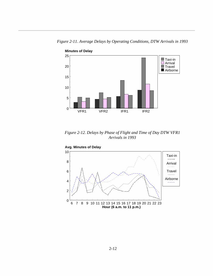
Although low ceiling and visibility are somewhat more common at DTW than BOS,average delays are less, even during IFR. Figure 2-11 shows average arrival delayduring IFR1 of about 13 minutes, versus an average of over 40 minutes at BOS.When examining specific days of poor weather at the two airports, BOS shows manymore very bad days when delays of a half hour to hour are routine. Such days aregenerally uncommon at DTW, as the parallel runways do not lose independent opera-tions under IFR conditions. At BOS, IFR conditions result in single runway opera-tions and their associated large flight capacity reductions.
Figure 2-10. Detroit Haze by Hour
6 7 8 9 10 11 12 13 14 15 16 17 18 19 20 21 22 23 2410
12
14
16
18
20
22
24
26
Hour (6 a.m. to 12 p.m.)
Percent Haze Occurence
2-12
Figure 2-11. Average Delays by Operating Conditions, DTW Arrivals in 1993
VFR1 VFR2 IFR1 IFR20
5
10
15
20
25Minutes of Delay
Taxi-inArrivalTravelAirborne
Figure 2-12. Delays by Phase of Flight and Time of Day DTW VFR1Arrivals in 1993
6 7 8 9 10 11 12 13 14 15 16 17 18 19 20 21 22 230
2
4
6
8
10
Hour (6 a.m. to 11 p.m.)
Avg. Minutes of Delay
Taxi-in
Arrival
Travel
Airborne

Characteristics of Weather and Delays at BOS and DTW
2-13
SUMMARY AND CONCLUSIONS ON OBSERVED DELAYS
We summarize our preliminary analyses in these terms:
◆ For all airport and month combinations considered, the days with the worst arri-val delay performance were always associated with IMC. Instances in whichweather-reduced capacity produced delay were identifiable in all airport andmonth combinations.
◆ For all airport and month combinations considered, days with the best arrivaldelay performance were always associated with VFR1.
◆ In most cases, interactions among weather, capacity, demand, and delay can befollowed in detail.
◆ Different phenomena appear to be most significant for delays at the two airportsstudied; the degree to which meteorological conditions are associated with delayvaries from airport to airport.
◆ Arrivals that occur in IMC account for significant fractions of total arrival delay.The fraction of arrivals that occur in IMC varies significantly from airport to air-port.
We conclude the following:
◆ There are enough identifiable arrival capacity-reduction mechanisms to makepossible an effective analysis of the specific effects of the TAP technologies.
◆ Identifiable arrival capacity-reduction mechanisms differ from airport to airportand enable the effective study of benefits of all three TAP technology groups.
◆ Even though IMC prevails only about 10 percent of the time overall, a significantfraction of delay is associated with IFR arrivals at many, if not most, airports.

3-1
Chapter 3
Modeling Airport Capacity
OVERVIEW
One of the key objectives of this analysis is to use an appropriate model to estimatethe capacity of an airport as a function of weather, FAA procedures, and the level oftechnology available. We define airport capacity as a Pareto frontier of arrivals perhour, versus departures per hour. This frontier is the boundary of the set of points atwhich arrival rate and departure rate can be simultaneously increased.
Figure 3-1 gives an example capacity curve, taken from data prepared for an FAAstudy. The figure indicates that, when departures are given priority, Newark Interna-tional Airport can accommodate up to 57 departures per hour. Up to 46 arrivals perhour can be integrated into the departure stream while maintaining that departure rate.Increasing the arrival rate above 46 per hour can only be done by decreasing the de-parture rate, up to an arrival rate of 50 per hour. This is the airport maximum arrivalrate: Up to 48 departures per hour can be accommodated while maintaining that rate.(An airport capacity curve is not necessarily made up of straight-line segments likethe example.)
Figure 3-1. Example Airport Capacity
0 20 40 600
20
40
60
Arrivals/hour
EWR

3-2
Actual airport capacity varies with, among other factors, ceiling, visibility, windspeed and direction, and the kinds of aircraft using the facility so that a completespecification of airport capacity is a family of curves like that of Figure 3-1.
This study requires the development of estimates of airport capacity, such as thatshown in Figure 3-1, and their modification to reflect the impacts of the TAP systems.To do so, it is necessary to use an appropriate model that can estimate capacity as afunction of weather conditions and those capacity parameters affected by the TAPsystems. The resulting capacity estimates can then be used to calculate the reductionin delay for a given level of demand.
PARAMETRIC CAPACITY ANALYSES AND SIMULATIONS
Several models of airport capacity have been developed over the past three decades.These can generally be classified into two categories, simulations and analytical mod-els. The simulation approach uses a highly detailed representation of airport and air-craft operations and extensive Monte Carlo iterations are required to analyze theimpact of changes in runways, taxiways, procedures, and technological capability onairport capacity and delay. These simulations are usually required when evaluatingchanges to the physical layout of an airport or adjustments to its airspace. They re-quire a great deal of data to operate, thereby requiring several months to complete astudy of a single airport.
Analytical models use a limited set of parameters and produce results with a singleexecution. Analytical models are also used to estimate the impact of changes in pro-cedures and technology on airport capacity. Because they do not require a highly de-tailed description of all aspects of airport operations or multiple runs, analyses of asingle airport can often be completed in much less time than a simulation would re-quire but with similar confidence in the results. The challenge in using an analyticalairport model is specifying the parameters that reflect the impact of the procedures ortechnologies to be evaluated. The parameters commonly used for airport capacityanalysis are miles in trail separations, arrival and departure runway occupancy times,the standard deviation of interarrival times (IATs), and aircraft mix. To the extentthat parameters such as these can accurately reflect the effects of the TAP systems, ananalytical model is ideal for the benefits analysis of this study. Analytical models donot, however, provide reliable insight into complex issues related to ground move-ment or detailed airspace operations. The most commonly used analytical model isthe FAA Airfield Capacity Model; we performed an extensive evaluation of it for thisstudy.

Modeling Airport Capacity
3-3
The approach used in the FAA Airfield Capacity model satisfies some, but not all, ofthe analytical requirements for this study. Most importantly, the model does not pro-vide adequate mechanisms for incorporating the several effects of the TAP systems.For example, many of the TAP technologies provide advanced automation tools topilots and controllers that will enable them to decrease the separation and improve thepredictability of the spacing between arriving aircraft. In modeling terms, this auto-mation reduces the variation in IAT. The FAA Airfield Capacity model enables usersto input a standard deviation of IAT. But, to evaluate the TAP systems analysis, weneed a model that derives the distribution of IAT in a rigorous fashion. Other TAPautomation improves the quality of information available to controllers and speedscommunications. Neither of these effects can be incorporated cleanly into the FAAmodel.
To overcome these deficiencies, LMI developed a new analytical model of runwayand airport capacity that incorporates parameters related to the TAP systems. TheLMI runway capacity model takes an air traffic controller-based view of airport op-erations. The limitations on the quality of information accessible to the controller—such as aircraft position and speed—directly affect the spacing required for safe op-eration of aircraft streams. Similarly, delays in communications affect spacing re-quirements through the need to provide sufficient time for the controller to provideinstructions to aircraft.
Table 3-1 lists the key parameters used in the LMI Runway Capacity Model and theFAA Airfield Capacity Model. The important differences in the lists are those thataffect the distribution of IAT. The LMI model estimates the distribution of IAT fromthe aircraft mix, the standard deviation in approach speed, the standard deviation inwind speed, and the standard deviation in position uncertainty. In the FAA model, theuser simply inputs a value for the standard deviation of IAT. The different approachused by the two models is important for analyzing TAP since some of the crucial TAPsystems, such as CTAS-FMS integration coupled with DGPS, will improve the qual-ity of information available to the controller and, hence, reduce some of those uncer-tainties. The precise impact of those reduced uncertainties requires a rigorousanalysis to determine their potential effect on the distribution of IAT. Appendix Adescribes the derivation of the LMI runway capacity model in greater detail and pro-vides the Pascal code used to execute it.

3-4
Table 3-1. Capacity Model Parameters—Comparison
LMI-Runway Capability Model FAA-Airfield Capability Model
pi, fraction of aircraft in class I pi, fraction of aircraft in class I
Sij, miles-in-trail minima Sij, miles-in-trail minima
Vi, approach speeds Vi, approach speeds
D, common path length D, common path length
Rai, arrival ROT Rai, arrival ROT
σAi, s.d. of arrival ROT σAi, s.d. of arrival ROT
Rdi, departure ROT Rdi, departure ROT
σDi, s.d. of departure ROT σDi, s.d. of departure ROT
Dd, distance-to-turn on departure TD, departure time intervalσD, s.d. of departure time interval
Vdi, departure speed
σDi, s.d. of departure speed σTA, s.d. of interarrival time
σx, s.d. of position uncertainty
σVi, s.d. of approach speed
σw, s.d. of wind speed
c, mean communications delay c, mean communications delay
σc, s.d. of communications delay
Note: Subscripts indicate variation with aircraft class. ROT = runway occupancy time;s.d = standard deviation.
Figure 3-2 shows an example of the runway capacity model output. The chart depictsa baseline arrival-departure capacity based on current arrival separation requirements.The outer capacity line reflects the impact of reducing those separations for all aircraftclasses. While the chart is only illustrative, it does show the important features of themodel:
◆ the tradeoff between arrivals and departures;
◆ direct treatment of the key TAP systems; and
◆ other effects, such as communications delay and aircraft mix.

Modeling Airport Capacity
3-5
The two study airports do not usually operate with only one active runway duringbusy periods. Accordingly, for most conditions the capacity of an airport must be es-timated by combining estimates of single-runway capacities into estimates for the ca-pacities of combinations of runways operated simultaneously.
It is possible to estimate capacities of combinations of runways analytically. The taskis trivial in some cases, such as when two runways are sufficiently separated that FAAregulations permit them to be operated simultaneously and independently. Parallelrunways separated by more than 4,300 feet usually meet that condition. In more com-plex cases, analytic models may be developed by modeling the effects of FAA proce-dures governing dependent runway operations.
The actual operation of runway configurations at large airports often involves a gooddeal of airport-specific practice. For example, when DTW is operating in the21L/21C/21R configuration, runway 21L is used for arrivals only, 21R is used for amix of arrivals and departures that depends on demand, and runway 21C is used fordepartures only. Figure 3-3 shows the runway layouts at DTW, along with informa-tion on runway length and separations. Figure 3-4 provides similar information forBOS.
Figure 3-2. Runway Capacity Model Output
0 10 20 30 40 50 60 70
70
60
50
40
30
20
10
0
Arrivals/hour
Current Value
Reference

3-6
Since in this study we estimate the capacities of a relatively limited set of airports. Itis both more efficient and more accurate to develop models of the specific runwayconfigurations actually used at these airports, in consultation with the controllers whooperate them, rather than to develop general multi-runway models and particularizethem to a given airport. The airport capacity models used for this study were builtthat way.
The models generate estimates of airport capacity hour-by-hour based on the weatherconditions in effect on the airport surface during that time, and the level of technologyas reflected in the runway capacity model parameters. The sequence operates as fol-lows:
1. estimate runway capacity as a function of available technology;
2. estimate the capacity of the airport runway configurations based on currentweather and available technology;
3. determine the most effective runway configuration to use, based on esti-mated capacity and weather conditions;
4. generate an hourly series of airport capacities.
5. Appendix B provides more detailed information on the airport capacitymodels for BOS and DTW.

Modeling Airport Capacity
3-7
Figure 3-3. Detroit Figure from ASC Plan

3-8
Figure 3-4. BOS Airport Layout from ASC Plan

4-1
Chapter 4
Estimating Delay
The runway and airport capacity models described in Chapter 3 satisfy the analyticalrequirement to estimate airport arrival and departure capacity as functions of weatherand available technology. The next step is to estimate aircraft delays given airportcapacity and demand. Queuing models are used for this. Comparing the resulting de-lays with and without the TAP systems gives estimates of TAP’s impacts on delay.
QUEUING MODELS OF AIRPORT OPERATIONS
Many models of airports as queues are available. Malone1 describes the considera-tions affecting their design and cites several examples. Queues are usually defined byspecifying three features: the demand process, the service process, and the number ofservers. (Sometimes a fourth feature, the maximum number of members that thequeue may have, is added.)
The symbol “M” designates a Markov demand or service process, for which interarri-val times or service times have a Poisson distribution.2 Thus a queue described as“M/M/1” has Markov demand and service processes and one server. M/M/1 queuesare widely used to model airport arrival and departure operations.
M/D/1 is another queue model used in airport analyses. The “D” indicates determi-nistic service (i.e., all service times are equal to a given constant). M/M/1 queuestend to overestimate airport delays, and M/D/1 queues tend to underestimate them.The queue model designated M/Ek/1, where Ek indicates that the service times havethe Erlang-k distribution3 with parameter k, gives delays between the M/M/1 andM/D/1 results.
1 Malone, K. M., “Dynamic Queuing Systems: Behavior and Approximations for Individual
Queues and for Networks,” Section 1.2 and its references. Ph. D. dissertation, Sloan School of Man-agement, Massachusetts Institute of Technology, June 1995
2 The Poisson distribution is p t e t( ) = −λ λ
3 The Erlang-k distribution is p tk t
ke
kk t( )
( )
( )!=
−
−−λ λ
1
1

4-2
M/M/1, M/D/1, and M/Ek/1 all have relatively simple steady-state behavior when ca-pacity exceeds demand. Unfortunately, these are not particularly helpful for airportstudies because capacity is less than demand for many interesting cases—and also be-cause, as pointed out by Odoni and Roth,4 during busy periods airports rarely operateunder fixed conditions long enough to reach the steady state.
In principle, exact unsteady results for M/M/1, M/D/1, and M/Ek/1 queues can beevaluated numerically. This may, however, require unacceptably long computingtimes. That motivates searches for approximations that give useful results in reason-able times. We have found one such approximation, the fluid model, particularly use-ful. It is described in the following section.
THE FLUID APPROXIMATION MODEL
The fluid approximation for a single queue of length q, with mean input rate λ andmean service rate µ, is the solution of the equation
else. ,
( ) ,=− >−
+λ µλ µ
0
where
( )( ), ( ),x mx m x m
else− ≡ − − >
+ 00
which takes on the value of the mean queue length at the initial time.
If λ and µ are piecewise constant functions of time, then the fluid approximation for qis a piecewise linear continuous function (i.e., a spline of order two (possibly on aknot sequence that is a refinement of the knot sequence for λ and µ5). This fact al-lows simple numerical schemes to generate fluid approximations rapidly—this is thefluid approximation’s great advantage. The sense in which the fluid approximation forqueues and queuing networks is a rational asymptotic expansion is discussed by Man-delbaum and Massey6 and by Chen and Mandelbaum.7
4 Odoni, A. R., and E. Roth, “An Empirical Investigation of the Transient Behavior of Stationary
Queuing Systems,” Operations Research 31, pp. 432-455, 1983.5 The “knot sequence” of a spline is the set of points at which the function’s defining parameters
may change.6 Mandelbaum, A., and W. Massey, “Strong Approximations for Time-Dependent Queues,”
Mathematics of Operations Research 20, pp. 33-64, February 1995.

Estimating Delay
4-3
The fluid approximation generally gives useful approximations for airport delays thatare associated with utilization ratios, ρ λ µ≡ / , that are significantly greater than onefor extended periods. Boston’s Logan International Airport appears to be one atwhich such delays account for the bulk of total delays. Figure 4-1 compares the exactmean queue for a M/M/1 model of a reduced capacity period at BOS, with the fluidapproximation for the same period. The results show the approximation to be excel-lent, with a relatively constant difference that is readily calculated.
It is important not to use the fluid model when the utilization ratio, λ/µ, stays lessthan one, but very close to one, for extensive periods. In these cases, while the fluidmodel gives zero queue size, the actual queue may become significantly large. Theanalysis used in this study tests for these cases, and uses numerical integration to de-termine queue properties when they occur.
Modeling Arrival and Departure Demand
The previous chapter described how capacity can be estimated as a function ofweather and available technology. Airport operations demand is also a key part of
7 Chen, H., and A. Mandelbaum, “Discrete Flow Networks: Bottleneck Analysis and Fluid Ap-proximations,” Mathematics of Operations Research 16, pp. 408-446, 1991.
Figure 4-1. Exact Mean Queue and Fluid Approximation
5 10 15 20 25 30
200
150
100
50
0
Me
an
Nu
mb
er
in Q
ue
ue
Accuracy of R eservoir M odel
Eastern S tandard T im e
Exact Reservo ir

4-4
that analysis. For this study, we use hourly tower counts of arrivals and departuresduring representative days as the measure of demand placed on the airport. Since ac-tual operations on days with reduced capacity are significantly affected by the poorweather, we use the arrival and departure counts on VMC days with no delay as thebaseline demand for estimating delays on IMC days. That is, arrival delays on IMCdays are based on the assumed desired mix of arrivals and departures that is typicallyfound on VMC days.
The available demand data for BOS are the tower records of arrival and departures forMay 20, 1993 through February 5, 1995. Through a statistical analysis of the records,we identified six distinct demand patterns. These six patterns are: winter weekdays,winter Saturdays, winter Sundays, summer weekdays, summer Saturdays, and sum-mer Sundays. These days represent the regular weekly and seasonal variations in de-mand at BOS.
The demand data available for analyzing DTW are processed from ARTS tapes forthe week of July 16-22, 1995. Since the FAA controllers at DTW reported that de-mand does not vary much with the seasons at DTW, three representative days wereused to analyze DTW. These days are Saturday, Sunday, and Thursday in the week ofJuly 16-22, 1995.
These demand counts and patterns serve as the principal driving force for estimatingdelays in this study. This approach differs from the methods typically used in otherstudies, which usually measure delay as the difference between actual arrival time andsome scheduled time, such as from the OAG or a flight plan. The approach devel-oped in this study has two advantages: First, it directly estimates the delay attribut-able to IMC conditions, without reference to any possible “schedule padding” used bythe airlines. Second, the use of hourly counts reduces the computational burden con-siderably. Although some precision is lost by ignoring scheduling peaks within eachhour, this method preserves the overall estimate of delay reduction that is needed toprovide preliminary estimates of the benefits from the TAP program. Our interest isnot so much in the delay experienced by a specific flight as it is in the overall reduc-tion in delay experienced by all flights arriving at an airport.

5-1
Chapter 5
Estimating the Impacts of TAP Technologies onCapacity and Delay at BOS and DTW
This chapter shows how we applied the methods described above to analyze the ef-fects of implementing TAP technologies at BOS and DTW. The approach unfolds insix steps:
1. Select the model parameters that accurately reflect the technology states.
2. Calculate airport capacity as a function of weather and the level of avail-able technology.
3. Estimate the delay reduction from TAP for specific days and demandpatterns.
4. Devise a method to annualize the delay estimates.
5. Devise a method to estimate delays through the year 2015, with and with-out the TAP systems.
6. Translate the delay reductions due to TAP into airline operating cost sav-ings.
The remainder of this chapter describes the first five steps listed and Chapter 6 ad-dresses the methods for translating delay reductions into airline cost savings.
CAPACITY MODEL PARAMETERS AND THEIR
CORRELATION WITH TAP TECHNOLOGIES
In modeling airport capacity, we relied primarily on the LMI models described inChapters 3 and 4 . We did so because it is simpler to relate the TAP systems effectsto parameters of the LMI model than to parameters of the FAA capacity model andbecause documentation of the FAA model does not describe some important featuresin adequate detail. We did carry out a parallel modeling effort based on the FAAmodel to provide a comparison.
5-2
In this chapter, we describe the input parameters of the LMI capacity models and howthey are affected by TAP technologies. We first describe the five technology statesconsidered. Following that, we address the model parameters, how they relate to theTAP technologies, and what values are appropriate for each technology state.
THE FIVE TECHNOLOGY STATES MODELED
The five technology states modeled are a current reference consisting of the IFR con-ditions that exist today; a 2005 baseline, and three increments of TAP technology.
Current Reference. The model parameters for the Current Reference were obtainedlargely from FAA-EM-78-8A, Parameters of Future ATC Systems Relating to Ca-pacity/Delay, June 1978, and the Upgraded FAA Airfield Capacity Model, Volume 1(hereafter referred to as “the User’s Guide”), May 1981. These were supplemented byinformation from NASA and FAA personnel and with information from the Air Traf-fic Control Handbook, FAA 7110.65. The Current Reference uses the aircraft classi-fications and wake vortex separations defined in FAA Safety Notice N 7110.157, July16, 1996.
2005 Baseline. We assumed that the TAP systems would not be fielded and opera-tional until the year 2005, so that year was used as the baseline. Between now and2005, several enhancements to existing capabilities that are not part of TAP are ex-pected to become available for general use. The 2005 baseline assumes deploymentof the Center/TRACON Automation System (CTAS) and the implementation of theWide Area Augmentation System (WAAS). All aircraft are assumed to be equippedwith Global Navigation Satellite System (GNSS) equipment. The impact of thesetechnologies includes reduction in aircraft position uncertainties and a modest expan-sion of approach path alternatives.
TAP 1. The first TAP increment includes the Aircraft Vortex Spacing System(AVOSS) with wake vortex sensors and upgraded TCAS information on lateralspacing. We expect these elements, along with CTAS/GPS, to enable reduced sepa-rations for traffic behind B757 and heavy aircraft.
TAP 2. The second TAP increment includes the TAP 1 systems and adds technolo-gies being developed in the Low Visibility Landing and Surface Operations(LVLASO) program. LVLASO programs include the Dynamic Runway OccupancyMeasurement system (DROM), the Aircraft Rollout and Turnoff (ROTO) system, andthe Aircraft Taxi-Navigation and Situational Awareness (T-NASA) system. Specifictechnical capabilities include GPS precision landing capability plus any cockpit taximaps and sensor systems necessary to reduce arrival runway occupancy time (ROT).

Estimating the Impacts of TAP Technologies on Capacity and Delay at BOS and DTW
5-3
TAP 3. The third TAP increment includes TAP 1 and TAP 2, plus integratedCTAS/FMS. Integration assumes two-way CTAS/FMS data linking. In the TAP 3increment, CTAS would be operating “closed loop” with the current flight plans ofindividual aircraft based on data from the FMS. Moreover, the FMS will providehigh confidence that the plans will be carried out as described. Flight plan revisionswill be communicated both ways in real time. The precise knowledge of the relativepositions of all traffic will enable execution of specific “soda straw” flight paths toavoid wake vortices. The parametric result will be reduced uncertainty about aircraftstatus and intent that can be used to safely reduce IFR separations to VFR distances.
We discuss specific modeling parameters and the values they assume in the five tech-nology states in the following subsections.
Model Parameters and Their Relations to the Technology States
Table 5-1 lists the parameters used in the LMI runway capacity model. For compari-son, it also shows the parameters used in the FAA Airfield Capacity Model.
Table 5-1. Runway Capacity Model Parameters; Comparison
LMI-Runway Capacity Model FAA-Airfield Capacity Model
pi, fraction of aircraft in class ι pi, fraction of aircraft in class ιSij, miles-in-trail minima Sij, miles-in-trail minima
Vi, approach speeds Vi, approach speeds
D, common path length D, common path length
RAi, arrival ROT RAi, arrival ROT
σAi, s.d. of arrival ROT σAi, s.d. of arrival ROT
RDi, departure ROT RDi, departure ROT
σDi, s.d. of departure ROT σDi, s.d. of departure ROT
Dd, distance-to-turn on departure TD, departure time intervalσD, s.d. of departure time interval
VDi, departure speed
σDi, s.d. of departure speed σTA, s.d. of interarrival time
σx, s.d. of position uncertainty
σVi, s.d. of approach speed
σw, s.d. of wind speed
c, mean communications delay c, mean communications delay
σc, s.d. of communications delay
Note: Subscripts indicate variation with aircraft class. ROT = runway occupancytime; s.d. = standard deviation

5-4
Runway Configuration
As detailed in Chapter 3, the Airport Capacity Model estimates arrival and departurecapacity combining outputs from the LMI Runway Capacity Model according to op-erating rules provided by controllers at the subject airports. Estimating airport capaci-ties requires constrained super position of runway model results. The constraintsgenerally reflect air traffic control (ATC) operating procedures with items like timedelays for clearing intersections and distance minimums for interleaved departuresand arrivals. The airport models check interarrival times, runway clearing times, plusany additional constraint conditions, to insert departures between arrivals. Departuresare estimated in the same manner.
For each of the airports studied, the same runway configurations are used for the Cur-rent Reference, 2005 baseline, and the TAP increments. We assume that GPS andTAP technologies (particularly information for lateral spacing) will allow independentuse of parallel runways spaced greater than 2,500 feet apart. As it happens, neither ofthe two airports studied has runways in this class that are not also sufficiently widelyspaced for independent operation under present rules (i.e., ≥4,300 feet).
AIRCRAFT MIX
We currently model four classes of aircraft in the operational mix. The small, large,and heavy categories are classed by takeoff gross weight (TOGW) as shown in Table5-2. In addition to these standard categories, the Boeing 757 is added as a fourth air-craft class, between the large and heavy categories.
Table 5-2. Aircraft Weight Categories
Category Take-off Gross Weight
Small TOGW < 41,000
Large 41,000 < TOGW < 300,000
Heavy TOGW > 300,000
Average Official Airline Guide (OAG) data for 1993 provided the percentages of op-erations in each aircraft class. While the OAG does not include all flights (it excludesprivate, military, and some airfreight), we assumed that the ratios were reasonable forthe purpose of analysis. In the case of Boston, we acquired tower data that provided amore complete and accurate history of operations. The aircraft ratios derived from theBoston tower data did not differ significantly from those derived from the OAG data.
Estimating the Impacts of TAP Technologies on Capacity and Delay at BOS and DTW
5-5
ARRIVAL RUNWAY OCCUPANCY TIMES
Arrival runway occupancy times (ROTs) are required for each arrival runway mod-eled. Sufficient field data are not available for all configurations and conditions to bemodeled, so analytic techniques are necessary to provide the required model input.
Current Reference. We produced the Current Reference arrival ROTs using theanalytic method and values contained in the User’s Guide for the FAA Airfield Ca-pacity Model. We checked the results with ROT data when possible.
For dry normal, dry high-speed, and wet runway exits the User’s Guide provides ta-bles of exit ROT versus distance from runway threshold and cumulative probability ofexit use versus distance from runway threshold for each of four classes of aircraft(i.e., small, small jet, large, heavy). Total runway ROT for a given class of aircraft isdetermined by establishing the exit distances for the runway, entering theROT/distance table to determine exit ROT, entering the probability/distance table todetermine probability of exit use factor, multiplying the ROTs by the probability fac-tors, and finally adding up the results. In our analyses, we determined the exit dis-tances from the airport diagrams contained in the U. S. Terminal Procedures“approach plates.”8
The User’s Guide tables are constructed for distances that are integral multiples of1,000 feet. In order to enter other values and automate the ROT calculations, we gen-erated curve fits to the table values and incorporated them into a short computer pro-gram. This program speeds the analysis process and also enables direct comparisonof field data with the User’s Guide model.
Unfortunately, the agreement between the ROT tables and collected data is oftenpoor. The differences that exist are generally within one standard deviation of thedata sample means, but the data are scattered and the standard deviations are large.The table values for dry runways consistently agreed better with the measured datathan the table values for wet runways. Several researchers, supported by the sparsehistorical data taken under IMC conditions, report that there is little or no differencebetween VMC and IMC ROTs. Consequently, the dry runway values from the modelare used in all cases.
The standard deviation of arrival ROT is an input parameter for the capacity models.The standard deviation parameter covers both the variations in pilot performance forgiven exits and the variations in exit selection by the pilots. The pilot performance
8 U. S. Government Flight Information Publication, U. S. Terminal Procedures, Department of
Commerce.

5-6
uncertainty corresponds to uncertainty in the ROT versus distance tables in the User’sGuide. The exit choice uncertainty corresponds to uncertainty in the probability useversus distance tables in the User’s Guide. TAP technologies may lead to improve-ments in the pilot performance uncertainties, but exit use is dependent on many exter-nal issues such as gate location, dynamic taxiway congestion, and construction thatare not addressed by TAP.
Eight seconds is the value of arrival ROT standard deviation used for the CurrentReference based on FAA-EM-78-8A. Eight seconds is on the low end of availablefield data, but there is no compelling logic to justify selection of a higher value.
2005 Baseline. We do not expect arrival runway occupancy times or their uncertain-ties to change in the 2005 baseline.
TAP 1. The TAP 1 technologies will not affect runway occupancy times.
TAP 2. The TAP 2 environment includes wide deployment of integrated GNSS/roll-out and turn-off (GNSS/ROTO) capability plus electronic taxi maps. These technolo-gies are modeled by reducing arrival ROT by 20 percent for each class of aircraft. 9
The ROT uncertainty may be reduced due to improved landing precision, but themodel parameter was not changed because (1) it is difficult to separate pilotage un-certainties that may be reduced from exit selection uncertainties that are unaffected,and (2) the base value of ROT uncertainty is already on the low end of the data.
TAP 3. No further reductions in ROT beyond TAP 2 are assumed for TAP 3.
IFR MINIMUM INTERARRIVAL SEPARATIONS
The minimum interarrival separations are strong drivers of airfield capacity both inthe models and in the real world. The IFR baseline values we use are those containedin the Air Traffic Control Handbook, FAA 7110.65H. The IFR separations recentlywere modified by FAA N 7110.157 to require a 5 nautical mile (nmi.) separation forsmall aircraft following Boeing 757s. The VFR separations are taken from FAA-EM-78-8A and are reputedly based on unidentified “field data.” FAA-EM-78-8A is old,but no major change in either operations or modeling has occurred since it was pub-lished. In addition, we find that the FAA-EM-78-8A values are still commonly usedin analyses, and we have no data to justify using others. Interarrival separations aredivided by aircraft speed to produce minimum interarrival times.
9 Twenty percent ROT reduction (50 seconds to 40 seconds) is the LVLASO goal stated in the
draft Level III plan.

Estimating the Impacts of TAP Technologies on Capacity and Delay at BOS and DTW
5-7
There are two distinct reasons for FAA separations. The first is the requirement forcontrollers to safely manage aircraft given the available displays, communications,and data rates. This requirement is the reason for the fundamental 3.0 nmi. minimumseparation. The second reason for separation is wake vortex hazard. Wake vortexhazard is the cause of all separations greater than 3.0 nmi.
Current Reference. The current reference IMC minimum interarrival separations aregiven in Table 5-3. FAA 7110.65 allows 2.5 nmi. separations in place of the 3.0 nmi.minimums under conditions that include documented ROTs under 50 seconds. Onerunway at Detroit and all runways at Boston meet the requirements under dry condi-tions. Both airports revert to 3.0 nmi. minimums when the runways are wet. Sincerunways are normally wet during IMC conditions we use 3.0 nmi. minimum separa-tions during IFR. We use the 2.5 nmi. minimum for VMC 2 conditions when radarcontrol is required, but the runways are usually dry.
Table 5-3. Current Reference InterarrivalSeparations (in Nautical Miles)
Trail
Lead Small Large B-757 Heavy
Small 3.0 3.0 3.0 3.0
Large 4.0 3.0 3.0 3.0
B-757 5.0 4.0 4.0 4.0
Heavy 6.0 5.0 5.0 4.0
2005 Baseline. CTAS and universal GNSS will not change the minimum separa-tions.
TAP 1. The TAP 1 interarrival separation minimums are given in Table 5-4. Thewake vortex prediction/detection capability introduced in TAP 1 will enable moderatereductions in the separations behind large and heavy aircraft, but will not enable re-ductions below the 3.0 nmi. minimum.

5-8
TAP 2. The TAP 2 LVLASO technologies result in ROTs less than 50 seconds underall meteorological conditions and, thus, allow use of 2.5 nmi. minimum separations inplace of the 3.0 nmi. separations in Table 5-4.
Table 5-4. TAP 1 Interarrival Separations(in Nautical Miles)
Trail
Lead Small Large B-757 Heavy
Small 3.0 3.0 3.0 3.0
Large 3.5 3.0 3.0 3.0
B-757 4.0 3.5 3.5 3.5
Heavy 5.5 4.5 4.5 3.5
TAP 3. The TAP 3 implementation includes CTAS/FMS integration plus reliablesituation awareness Airborne Information for Lateral Spacing (AILS) that will enableoperation with the VFR (FAA-EM-78-8A) separations given in Table 5-5. We notethat significant changes in the roles of air controllers, pilots, and automation must beresolved before TAP 3 separations can be achieved.
Table 5-5. TAP 3 Interarrival Separations(in Nautical Miles)
Trail
Lead Small Large B-757 Heavy
Small 1.9 1.9 1.9 1.9
Large 2.7 1.9 1.9 1.9
B-757 3.5 3.0 3.0 2.7
Heavy 4.5 3.6 3.6 2.7
INTERARRIVAL TIME UNCERTAINTY
The interarrival time uncertainty, σTA, is an input parameter in the FAA model. Theuncertainty is expressed as the standard deviation, in seconds, of the interarrival time.One value of σTA is used for all aircraft classes and leader/follower pairs. The uncer-tainty time is multiplied by a probability factor and added to the minimum interarrivaltime to produce a working time interval that has high confidence of not violating the

Estimating the Impacts of TAP Technologies on Capacity and Delay at BOS and DTW
5-9
separation minimums. The normally used confidence is 95 percent with a corre-sponding factor of 1.65.
The LMI runway capacity model, as described in Chapter 3, has separate inputs foruncertainties in position, approach speed, and wind speed. The model applies theseuncertainties to the specific aircraft leader/follower pairs as they fly the approachcommon path (common path is discussed below). The model applies confidence mar-gins to the resulting uncertainties in interarrival time to ensure against violation ofminimums.
The LMI model results make clear the fact that interarrival time uncertainties varysignificantly with leader/follower characteristics and with common path length. Acomposite interarrival time uncertainty that corresponds to the FAA model σTA can becalculated as an output by the LMI model for comparison with the FAA model input.
Interarrival time “error” data are available from man-in-the-loop final approach spac-ing aids (FASA) simulations performed by NASA.10 In the FASA experiments forCTAS supported cases, the difference between the minimum arrival time predicted byCTAS and the arrival time achieved by the controller was calculated for each flight.In cases not supported by CTAS, the difference between the minimum allowed sepa-ration and the actual threshold separation was calculated for each flight. The differ-ences in the times for sequential flights were calculated and defined as the interarrivaltime errors. Means and standard deviations of the interarrival time errors were com-puted. With some caution, the standard deviations can be compared to σTA.
It must be kept in mind that the uncertainty values used in the models represent thecontroller’s view. Improvements in the knowledge of position using GNSS, for ex-ample, will not result in reduced separations unless the information is communicatedto the controller in a way he can use it (e.g., through CTAS to a final approach spac-ing aid).
Current Reference. The LMI values for the uncertainty parameters of approachspeed, position, and wind were selected in the light of discussions with pilots andcontrollers. These parameters, along with the common path length and Boston aircraftmix, lead to a composite 17 second standard deviation of interarrival time. The FAAmodel current reference interarrival time uncertainty is 18 seconds (one standard de-viation), taken from FAA-EM-78-8A. The values for all the parameters, plus the er-ror data from the NASA simulation are shown in Table 5-6.
10 Final Approach Spacing Aids (FASA) Evaluation for Terminal-Area, Time-Based Air Traffic
Control, Credeur, et al, NASA Technical Paper 3399, Dec 1993.

5-10
Table 5-6. Interarrival Time Uncertainty Parameters
Parameter Current 2005 TAP 1 TAP 2 TAP 3
LMI Model Approach Speed,σVi
(knots)
5 5 5 5 4
LMI Model Position, σX
(distance)
0.25
(nmi.)
100
(feet)
100
(feet)
100
(feet)
100
(feet)
LMI Model Wind Speed, σW
(knots)
7.5 7.5 7.5 7.5 5
LMI Composite Uncertainty
(seconds)
17 13 13 13 10
FAA Model IAT Uncertainty,σTA
(seconds)
18 12 12 12 8
NASA Interarrival Errors
(seconds)
15.4-18.8 8.2-13.9 NA NA NA
2005 Baseline. In the LMI model, the 2005 baseline is modeled by reducing the po-sition uncertainty, σx, to 100 feet, in view of the position accuracy afforded by GNSSand, as discussed below, reducing the common path length to 5 miles. These changesproduce a composite standard deviation of interarrival time of 13 seconds. For inputsto the FAA model, we estimate that CTAS and universal GNSS will improve the po-sition accuracy and correspondingly reduce the interarrival uncertainty from 18 to 12seconds. The data from the NASA simulations gave a range of 8.2 to 13.9 secondsfor interarrival errors when using CTAS and the best of the semiautomated spacingaids.
TAP 1. TAP 1 technologies are not expected to affect interarrival time uncertainties.
TAP 2. TAP 2 technologies are not expected to affect interarrival time uncertainties.
TAP 3. In the LMI model, TAP 3 technologies reduce wind speed standard deviationto 5 knots due to the ability of the integrated CTAS/FMS to plan optimized flightpaths. The remaining uncertainty is due to individual pilot and airline preferences,which may not conform to the optimum path. In TAP 3, the FMS will also reduce theuncertainty in approach speed due to the more precise speed control by the FMS andthe transmission of reliable intent information to the CTAS computer. In the FAA
Estimating the Impacts of TAP Technologies on Capacity and Delay at BOS and DTW
5-11
model, the integration of ATC and FMS in TAP 3 is expected to reduce the interarri-val time standard deviation to 8 seconds.
APPROACH SPEEDS
The values for approach speeds used in our analyses are slightly higher than those ofthe examples in the User’s Guide. We based our approach speeds on discussions withairport controllers about the approach speeds they observe. The approach speeds donot change with time or TAP technology.
WIND SPEED STANDARD DEVIATION
Wind speed standard deviation is an input for the LMI model. This parameter reflectstwo effects. First, winds vary with time, so that leader and follower generally experi-ence different winds. Second, winds aloft vary with altitude, and leader and followermay fly different approach profiles, which also causes the two aircraft to experiencedifferent winds.
DEPARTURE RUNWAY OCCUPANCY TIME
Departure ROTs are not addressed in FAA-EM-78-8A. The departure ROTs we usedare based on the examples in the User’s Guide. Departure ROTs are typically shortand do not limit airport capacity. Departure ROTs are not affected by eitherCTAS/GNSS or the TAP technologies.
The uncertainty in departure ROT appears in both models. The current referencevalue of six seconds (one standard deviation) is used for all cases. Departure ROTuncertainty may be reduced by improved taxi precision, but no reductions were madein the model because there was no basis on which to predict or defend a specificvalue.
DEPARTURE SEPARATIONS
Departure time separations are specified in the FAA model and shown in Table 5-7.In the LMI model, departure miles-in-trail minima (currently assumed to be the sameas arrival miles-in-trail minima) are imposed, as is a 60-second minimum time be-tween departure clearances implied by FAA 7110.65H. Two switchable parametersare included in the LMI model. The first implements the FAA radar control practicefor runways being used for both arrivals and departures of not releasing a departure ifthe next arrival is within 2.0 nmi.11 This flag is set when meteorological conditions
11 Air Traffic Control, FAA 7110.65H, paragraph 5-114, Note 1.

5-12
do not allow the controller to see the arrival at 2.0 nmi. from the threshold. The sec-ond parameter is a 2-minute hold for departing aircraft when the preceding departureis a heavy aircraft.12
Table 5-7. Current Reference DepartureSeparations in Seconds
Trail
Lead Small Large B-757 Heavy
Small 60 60 60 60
Large 60 60 60 60
B-757 60 60 60 60
Heavy 120 120 60 60
Current Reference. The current reference values shown in Table 5-7. are taken di-rectly from FAA 7110.65H restrictions.
2005 Baseline. The departure separation restrictions are not expected to change forthe 2005 CTAS/GNSS baseline.
TAP 1. The departure separation restrictions are expected to be reduced by the TAP 1AVOSS technology. In the TAP 1 case, for both the FAA and LMI models, all sepa-rations are expected to be 60 seconds based on the ability to confirm the absence ofwake vortices.
TAP 2. TAP 2 technologies offer no further improvement in departure separations.
TAP 3. TAP 3 technologies enable removal of the departure hold requirement that isimposed when arrivals are within 2 nmi. of the threshold. The change is due to thecontroller’s ability to accurately predict the movements of arriving aircraft regardlessof meteorological conditions.
COMMON PATH LENGTH
The common path length is the distance from the threshold up the extended centerlinewithin which the controller issues no further speed change directions. If a slower air-craft is following a faster aircraft the controller will establish the minimum spacing atthe beginning of the common path. In the capacity models, the common path length
12 Air Traffic Control, FAA 7110.65H, paragraph 3-155f.

Estimating the Impacts of TAP Technologies on Capacity and Delay at BOS and DTW
5-13
is multiplied by the difference in aircraft speeds to determine the additional separationthat occurs when a slower aircraft is following a faster aircraft. In the LMI model, theuncertainties in wind speed and approach speed are applied over the common path tocalculate interarrival time uncertainty for all aircraft. Reductions in the common pathreflect physical reductions in the common path due to curved/angled approaches.
Current Reference. An IFR common path length of 6 nmi. is used for all aircraft.This value is taken from both FAA-EM-78-8A and the User’s Guide.
2005 Baseline. GNSS, like MLS, should allow curved and angled approaches with areduced common path. While we do not believe large reductions will be made formany years, if ever, we do expect to see modest approach path optimizations withCTAS/GNSS operation. We assume these will result in a 1 nautical mile reduction inthe common path (6 nmi. to 5 nmi.) due to modest adjustments to approach flightpaths.
TAP 1. TAP 1 technologies will not further reduce the common path.
TAP 2. TAP 2 technologies will not further reduce the common path.
TAP 3. Integrated CTAS/FMS technologies will enable both extremely accurate pre-diction of aircraft performance and use of curved/angled approach paths, but theseimprovements are too uncertain to warrant further reductions in the common path atthis time.
CROSSING RUNWAY ARRIVAL/DEPARTURE SEPARATION
This parameter is the amount of time the release of a departing aircraft is held up afteran arriving aircraft has crossed the threshold of a crossing runway. We use 5 secondsfor near-end crossing runways based on discussions with Boston controllers. We use30 seconds for far-end crossing runways to ensure that the arriving aircraft are notgoing around, but this value has not been confirmed with controller personnel. Thecrossing runway separation parameter is not affected by CTAS/GNSS or TAP tech-nologies.
Runway Model Results
Table 5-8 displays the LMI and FAA model results for a single runway during IMC.The runway modeled is Boston 4-Right, which is ILS-equipped. The good agreementwith the FAA Capacity Model for the maximum arrival capacities and the affirmationof the results by Boston controllers as described in Appendix A give sufficient confi-dence in the LMI model to use it for the full airport capacity analysis. The disparity

5-14
between the LMI model and the FAA model for departures (and, consequently, 50:50estimates) is not a major concern because the FAA model is known to overestimatedepartures.
Table 5-8. Comparison of LMI and FAA Capacity Model Results for a SingleRunway at BOS
Operating ConditionCurrent
Reference 2005 Baseline TAP 1 TAP 2 TAP 3
Maximum Arrivals LMI (arrivals/departures) FAA (arrivals/departures) EPS (arrivals/departures)
32/831/2728/8
34/534/25
36/236/24
39/439/25
52/1752/9
50:50 Operation LMI (arrivals/departures) FAA (arrivals/departures) EPS (arrivals/departures)
25/2530/3023/23
25/2531/31
25/2531/31
27/2733/33
39/3935/35
Maximum Departures LMI (arrivals/departures) FAA (arrivals/departures) EPS (arrivals/departures)
0/430/56
10/40
0/430/56
0/440/60
0/480/60
0/550/60
Note: The FAA Engineered Performance Standards (EPS) estimates are for a single runway, notspecified.
TIME SERIES OF WEATHER AT BOSWe used the NCDC data to generate files of hourly data on ceiling, visibility, windspeed, wind direction, and temperature at BOS for 26 years: 1961 to 1964, and 1969to 90. Records for 1965 to 1968 were omitted because the NCDC records for thoseyears give data only every 3 hours.
For each year, we identified the days on which there was at least one hourly report ofIMC conditions, in the hours 06:00 to 22:00 Eastern Standard Time. That is the pe-riod during which capacity reductions are most likely to cause significant delays. Foreach day thus identified, we extracted hourly data for 06:00 through 03:00 the fol-lowing day. These 22-hour periods were adequate for queues to return to zero formost of the IMC days.
We analyzed the IMC day records in detail, using the modeling approach described inChapters 3 and 4. While the IMC days account for most of the delay at BOS, there issome contribution from other days. To account for this, we identified a set of VMCdays and computed the average delay for these days with the full M/M/1 model for

Estimating the Impacts of TAP Technologies on Capacity and Delay at BOS and DTW
5-15
each year studied. Then we added the product of the number of days that were VMCand the average delay on VMC days, to the total delay for the bad days (estimatedfrom the reservoir model). The VMC days corrections were small, usually around 15percent of the total delay.
TIME SERIES OF WEATHER AT DTWWhen we applied the procedure used at BOS to DTW, we found qualitatively differ-ent results that caused us to modify the approach. Both delay data and the models in-dicate that delays at BOS are largely due to bad days. Delays at DTW, however, aremuch less dominated by days with substantial periods in which capacities are signifi-cantly below demands. A much greater fraction of delays at DTW, approaching 50percent, comes from days on which demand sometimes approaches capacity, but doesnot exceed it.
To cope with this different pattern, we treated DTW by considering all the days of theyear, using as our inputs weather data from 06:00 Local Standard Time (LST) through03:00 LST the following day. First, we generated the predictions of the reservoirmodel for all days of the year, for 06:00 LST to 03:00 LST the following day. Thenwe scanned all days for cases in which demand approached capacity from below. Wecomputed delays for each such day by the full M/M/1 differential equations.
We also identified a set of four good days, one from each quarter of the year. Weevaluated delays for these days with the M/M/1 equations, and used the average ofthese delays to represent delay on a good day.
We then accumulated delays for each day as follows: For a day on which demand ap-proached capacity from below, we used the M/M/1 result. For all other days, we usedthe sum of the good-day delay and the reservoir model.
The reservoir model gives zero delay except when demand exceeds capacity. On daysin which demand exceeds capacity for extended periods, the reservoir model predictssignificant delays and, as is discussed in Chapter 4, is a good approximation to thefull M/M/1 result. Thus, the sum of the reservoir model and the representative good-day delay is close to the good day figure, except when demand significantly exceedscapacity. For those days, the sum is close to the M/M/1 result.
FUTURE DEMAND AT BOSThe next step is to calculate a demand series for the years 2005 through 2015 whenthe TAP systems will be operating at BOS and DTW. The FAA Terminal Area Fore-

5-16
cast predicts that the total number of operations at BOS in 2005 will be 11 percentgreater than the number in 1993. As an estimate of demand in 2005, we increasedeach demand value in the six BOS seasonal demand patterns by 11 percent. Modelresults for 26 years of weather data at BOS were calculated.
We input the weather time series just described above into the capacity models usingthe parameters representing the five technology states. This gave five sets of capacitytime series.
These capacity estimates are then input into the queue models to generate the delayestimates from the baseline cases and the three TAP implementations.
Discussion
The results show that the pattern of estimated relative benefits from the TAP tech-nologies is quite consistent over 26 years of varying weather. Implementing only theTAP 1 technologies in 2005 would recover about half the increase in delay occa-sioned by going to 2005 demand levels with only the capacity improvements to beexpected from planned CTAS implementations. That is, this implementation wouldlead to about an 9 percent increase in delays over 1993 levels.
Implementing the TAP 2 technologies by 2005 would give a substantial decrease inIMC delays over 1993 levels, of about 22 percent. Implementing the TAP 3 tech-nologies would reduce IMC delays yet more significantly, by about 60 percent (i.e.,this would bring delays on IMC days to about 40 percent of 1993 levels).
RESULTS AT BOS FOR 2015This section describes our method of modeling effects of the TAP technologies atBOS in 2015.
Weather Data
Because the year-to-year results for 2005 implementations scatter so little, we esti-mated the results of implementations in 2015 from weather data for a single, typicalyear rather than by repeating the analyses for all 26 years. We chose 1982 for the rep-resentative year, because that year’s five values of IMC delays for current, 2005, TAP1, TAP 2, and TAP 3 conditions are closest to the 26-year means of these results. Weprefer to use the weather of an actual year rather than some average of the 26-yearweather data, because the averaging might construct implausible weather data.

Estimating the Impacts of TAP Technologies on Capacity and Delay at BOS and DTW
5-17
Demand Data
Demand data for 2015 were generated by growing the year 2005 demand at rates pre-scribed in the FAA Terminal Area Forecast (TAF) for the years 2001 to 2005. TheTAF shows BOS operations growing at an essentially constant rate of 1.5 percent peryear. Applying 10 years growth at the average of the 2001 to 2005 rates to the TAF2005 operations forecast leads to an estimate of 2015 demand that is 29 percentgreater than the 1993 demand. Accordingly, to estimate 2015 demand, we applied a29 percent increase to the six representative seasonal demand patterns used to analyzeBOS.
The 2015 demand data were input into the BOS capacity model. Table 5-9 displaysthe results for 2015 along with the results for current and 2005 baseline conditions(based on 1982 weather year).
Table 5-9. Annual Aircraft Arrival Delay at BOS(Millions of Minutes)
TechnologyState
1993 2005 2015
Current 5.5 6.8 12.2
TAP 1 – 5.9 10.8
TAP 2 – 4.8 8.9
TAP 3 – 2.1 4.2
MODEL RESULTS AT DTWThis section describes our results for DTW.
Weather Data
Because the results for 26 years at BOS varied so predictably with weather, we de-cided to identify a representative year of weather data for DTW and treat that year.The mean number of hourly reports of IMC at DTW for the 20 years 1971 to 1990 is1,157. The year 1985 was close to that value, and that year of weather data was usedas the weather input for DTW.

5-18
Demand Data
We based the demand data for 2005 and 2015 on the demand profiles used for thebaseline estimates. As with BOS, we estimated future demand at DTW using datafrom the FAA TAF. For 2005 patterns, we multiplied each demand value in our threepatterns by the ratio of total operations forecast for DTW in 2005, to that same num-ber for the year 1995. The TAF forecast shows total operations at DTW increasingby roughly 1.5 percent annually for 2000 to 2005. To estimate total operations in2015, we continued this rate of growth. The TAF predicts a 22 percent increase intotal operations at DTW from 1995 to 2005. Our extrapolation of the TAF predic-tions leads to an estimate of a 36 percent increase from 1995 to 2015.
We input the weather data to our DTW capacity model, for each of five parameter setsrepresenting technology in 1995, in 2005, and in 2015 with TAP 1, TAP 2, and TAP 3implementations. We then used the resulting capacity time series with demand timeseries just described, to estimate aircraft-minutes of delay at DTW for the five tech-nology states. Table 5-10 shows the results.
Table 5-10. Aircraft Delay at DTW for TAPImplementations (in Millions of Minutes)
CurrentReference
1995 2005 2015
Baseline 1.1 1.6 2.8
TAP 1 – 1.5 2.6
TAP 2 – 1.4 2.0
TAP 3 – 1.1 1.4
Discussion
The models indicate that DTW experiences significantly less delay than BOS. Thisresult is consistent with the relative frequency of delays currently experienced at thesetwo airports: The ratio of the predicted total delay at BOS to total delay at DTW incurrent conditions is roughly 4:1. This is also the ratio implied by delay data in the1994 FAA System Capacity Report.
The reason for the difference is not that DTW has less IMC than BOS; in fact, it hasmore, as shown by the discussions in Chapter 2. Nor is it the reason that DTW hasless traffic; while DTW had about 20 percent less traffic than BOS in 1993, opera-tions at DTW are forecast to increase faster than at BOS. In 2005 and 2015, DTW isforecast to have slightly more operations than BOS. The principal reason for the dif-

Estimating the Impacts of TAP Technologies on Capacity and Delay at BOS and DTW
5-19
ference is that the parallel runways at DTW are sufficiently widely spaced that theycan continue independent operations in IMC, while that is not the case at BOS. ThusBOS loses much more capacity in IMC than does DTW.
The analysis shows that the TAP systems should reduce delay at DTW, but not asmuch as at BOS. The reason for this appears to be that delays at BOS are largely dueto bad days on which demand significantly exceeds capacity for substantial parts ofthe day while there are much fewer such days at DTW. TAP is more effective onthose bad days than on the ordinary days, and ordinary days are more important todelay at DTW than at BOS.

6-1
Chapter 6
Converting Estimated Delays Into Air Carrier Costs
This chapter details how the costs of the delays were determined.
SOME DEFINITIONS
Direct operating costs (DOCs) include flight crew costs (e.g., salaries, bene-fits/pensions, payroll taxes, and personnel/training expenses); fuel and oil costs(including taxes); maintenance costs (including maintenance overhead); insurance andinjuries/loss/damage charges; aircraft rentals; and aircraft depreciation/amortizationcharges.
Variable operating costs (VOCs) are DOCs minus aircraft rentals and aircraft depre-ciation/amortization charges. Aircraft rentals and depreciation/amortization are ex-cluded from VOC because they reflect the passage of time (and hence are sometimescalled period costs) rather than how intensively and/or efficiently aircraft are oper-ated.
Block time is measured from when the aircraft first moves under its own power at thedeparture airport until it comes to rest at the arrival airport. Block time is thereforemore inclusive than flight time, which is measured from takeoff to landing.
FORM 41 DATA
Data collected by the Department of Transportation (DOT) from major, national, andlarge regional airlines at the equipment level of detail cover substantially all of thescheduled passenger traffic that occurs in the United States.
Using actual cost and traffic data for this analysis has the advantage of capturing howairframe/engine combinations are actually used by the airlines and the resources con-sumed to operate them that way. The actual data also reflect the effects of factorssuch as airline routing/scheduling decisions and airport/airspace congestion.
For the purposes of this analysis, we subdivided commercial passenger aircraft intothree categories: turboprops, short-haul jets, and long-haul jets. A 1,000 mile averagestage length (ASL) range is a fairly natural breakpoint for short- versus long-haul jet

6-2
aircraft. The most important cost and operating statistics for these three groups ofaircraft are summarized in Table 6-1.
Table 6-1. Passenger Airline Operating Statistics
Category
Share ofDirect
OperatingCosts (%)
Share ofVariable
OperatingCosts (%)
Shareof FuelCosts(%)
Share ofASMsFlown(%)
Share ofRPMsFlown(%)
AverageSeatsper
Aircraft
AverageStageLength(miles)
Turbo-props
1.9 1.6 0.9 0.7 0.6 33 179
Short-haul jets
53.4 54.3 50.9 48.1 45.2 131 580
Long-haul jets
44.7 44.1 48.2 51.2 54.2 246 1,653
As shown in Table 6-1, turboprops and short-haul jets consume a higher proportion oftotal costs relative to their shares of revenue passenger miles flown. This occurs forseveral reasons. Because short-haul flights spend relatively less time at cruise at effi-cient conditions compared with the higher costs (in time and fuel) of—taking off, ma-neuvering out of the departure terminal area, climbing to altitude, maneuvering intothe arrival terminal area, and landing—their relative costs are higher than long-haulflights. Second, load factors on turboprops and short-haul jets are lower than forlong-haul jets ( 51.6 percent and 59.8 percent versus 67.3 percent, respectively).
It is also important to note the positive correlation between average seats per aircraftand the average stage lengths flown. Consequently, the higher the proportion ofshort-haul flights into an airport, the larger will be the expected share of turbopropsand smaller jet aircraft.
ESTIMATED SYSTEM-WIDE DELAY COSTS PER BLOCK
MINUTE
To estimate upper and lower bounds for system-wide delay costs per block minute,we defined pessimistic and optimistic scenarios. For the pessimistic scenario, weadded an allocated share of cabin crew costs to the reported equipment-level DOCand divided by block minutes of time. This estimate of delay cost includes fuel costsplus aircraft depreciation/amortization and rental costs. It therefore implicitly as-sumes that all arrival delay is incurred in the air and that some incremental capitalcosts are incurred during the delay period. For the optimistic scenario, we started

Converting Estimated Delays Into Air Carrier Costs
6-3
with VOC (therefore excluding aircraft depreciation/amortization and rental costs),once again added an allocated share of cabin crew costs, subtracted fuel costs, anddivided by block minutes of time. This estimate implicitly assumes that all arrivaldelay is incurred on the ground (where consumption of fuel is much lower than in theair) and that depreciation/amortization and rental costs would have to have been paidwhether the aircraft was productively employed or not and therefore should not becharged against the delay. It is therefore appropriate to think of these two scenarios asthe upper and lower bounds, respectively, on the true costs of aircraft delay experi-enced by the airlines. No attempt was made to estimate the costs to the airlines or theflying public resulting from canceled flights. Estimated system-wide delay costs perblock minute are summarized in Table 6-2.
Table 6-2. System-wide Delay Costs by Type of Aircraft
Type of Aircraft
Pessimistic Case:Direct operatingcosts + cabin
crew cost by block time ($)
Optimistic Case:Variable operatingcosts + cabin crew
cost - fuel cost by block time ($)
Turboprop 11.09 6.15
Short-haul jet 35.36 20.29
Long-haul jet 68.94 36.73
Weighted average 43.26 24.01
OPERATIONS AT BOSTON’S LOGAN INTERNATIONAL
AIRPORT AND DETROIT’S WAYNE COUNTY AIRPORT
In order to gain insights into the composition and significance of the various types ofaircraft that are flown into the Boston Logan and Detroit Wayne County airports, weextracted scheduled flight data for January 1993 from the Official Airlines Guide(OAG) North American and Worldwide merge files. These data sources are computertapes that list all of the flights that were scheduled to occur during a certain period oftime, listed by carrier and type of equipment. The OAG flight data were combinedwith DOT Form 41 load factor and stage length statistics to estimate the number ofpassengers and revenue-passenger miles flown. Summary results are shown in Tables6-3 and 6-4.
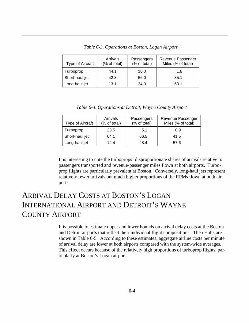
6-4
Table 6-3. Operations at Boston, Logan Airport
Type of AircraftArrivals
(% of total)Passengers(% of total)
Revenue PassengerMiles (% of total)
Turboprop 44.1 10.0 1.8
Short-haul jet 42.8 56.0 35.1
Long-haul jet 13.1 34.0 63.1
Table 6-4. Operations at Detroit, Wayne County Airport
Type of AircraftArrivals
(% of total)Passengers(% of total)
Revenue PassengerMiles (% of total)
Turboprop 23.5 5.1 0.9
Short-haul jet 64.1 66.5 41.5
Long-haul jet 12.4 28.4 57.6
It is interesting to note the turboprops’ disproportionate shares of arrivals relative topassengers transported and revenue-passenger miles flown at both airports. Turbo-prop flights are particularly prevalent at Boston. Conversely, long-haul jets representrelatively fewer arrivals but much higher proportions of the RPMs flown at both air-ports.
ARRIVAL DELAY COSTS AT BOSTON’S LOGAN
INTERNATIONAL AIRPORT AND DETROIT’S WAYNE
COUNTY AIRPORT
It is possible to estimate upper and lower bounds on arrival delay costs at the Bostonand Detroit airports that reflect their individual flight compositions. The results areshown in Table 6-5. According to these estimates, aggregate airline costs per minuteof arrival delay are lower at both airports compared with the system-wide averages.This effect occurs because of the relatively high proportions of turboprop flights, par-ticularly at Boston’s Logan airport.

Converting Estimated Delays Into Air Carrier Costs
6-5
Table 6-5. Airport-Specific Cost per Minute of Arrival Delay
AirportArrival delay cost per minute,
upper bound ($)Arrival delay cost per minute,
lower bound ($)
Boston, Logan 29.06 16.21
Detroit, WayneCounty
33.82 19.01
System-wide 43.26 24.01
POTENTIAL SAVINGS FROM TAP TECHNOLOGIES
As described in Chapter 4 of this report, when the level of operations is combinedwith the airport capacity (which is itself affected by technology and weather), the LMIAirport Capacity Model yields reliable predictions of arrival delay experienced by theairlines. As shown in Table 6-6—given the 1993 level of airport operations, a year’sworth of representative weather, and existing technology—the predicted levels of ar-rival delay measured in aircraft minutes are 5.5 million and 1.1 million for Bostonand Detroit, respectively. Because of relatively modest growth to the year 2005 inairport operations at Boston, arrival delay is expected to grow there at a much slowerrate compared with Detroit. From 2005 to 2015, however, the compound growthrates of arrival delay are predicted to be 6.0 percent and 5.7 percent for Boston andDetroit, respectively.
Table 6-6. Aircraft Minutes of Arrival Delay
Airport 1993 2005 2015Compound growth rate,
2005 to 2015 (%)
Boston 5,548,684 6,786,192 12,194,081 6.0
Detroit 1,104,555 1,614,681 2,806,667 5.7
Using the arrival delay cost factors discussed previously, it is possible to convert pre-dicted aircraft-minutes of arrival delay into airline costs. For Boston in 1993, thesearrival delay costs are estimated at between $89.9 million and $161.2 million, while atDetroit in 1993, the lower and upper bounds are $21.0 million and $37.4 million.Airline arrival delay costs grow modestly to the year 2005, but accelerate quite dra-matically thereafter. By 2015, predicted airline arrival delay costs at these two air-ports are expected to more than double from the 1993 levels, holding technologyconstant.

6-6
Table 6-7. Airline Arrival Delay Costs($ Millions)
Airport 1993 2005 2015
Boston, upper bound 161 197 354
Boston, lower bound 90 110 198
Detroit, upper bound 37 55 95
Detroit, lower bound 21 31 53
If TAP technologies ultimately prove to be successful and are implemented by theyear 2005, the LMI Airport Capacity Model predicts that there will be significantimprovements in airport capacity at the Boston and Detroit airports, particularlyduring periods of inclement weather. Consequently, certain proportions of predictedarrival delay are avoided as the TAP increments are progressively added. Bymultiplying the predicted reduction in aircraft-minutes of arrival delay times theairport-specific delay cost factors, yearly benefits in terms of reduced airline arrivaldelay costs can be estimated for each year from 2005 to 2015. Using a 5 percent realinterest rate, these future benefits can be discounted back to the present so that theymay be compared with the costs of the TAP program. We use a real interest rate (asopposed to a nominal one) because future benefits are measured in constant 1995dollars. We selected a 5 percent interest rate because of the risk of R&D investmentsand the uncertainty of future payoffs. As shown in Table 6-8, the biggest payoffs atBoston and Detroit are from TAP Increments 2 and 3.
Table 6-8. Present Value of Arrival Delay Costs Avoided ($ Millions)
AirportTAP Increment
1TAP Increment
2TAP Increment
3 Total
Boston, upper bound 165 236 542 937
Boston, lower bound 92 129 302 523
Detroit, upper bound 24 62 70 157
Detroit, lower bound 14 35 39 88

Converting Estimated Delays Into Air Carrier Costs
6-7
ADDITIONAL DATA NEEDED
The conclusions of the analysis appear to be robust with respect to the effects ofweather variations and the results are consistent with delays currently experienced atthe two airports. However, the following additional analysis and data collectionwould benefit the analysis;
1. The available data on arrival runway occupancy time are sparse and toounreliable to provide consistent insight into current operations, much lessthe impact of advanced technologies. NASA and the FAA should collabo-rate under the LVLASO program to collect arrival ROT data during peaktraffic operations under VMC and IMC conditions. While this studyshows that ROT will be a significant constraint as arrival separation dis-tances shorten, the study cannot clearly identify at what point the con-straint will be binding without better ROT data.
2. The effects of CTAS and CTAS-FMS integration on the distribution ofinterarrival time are important and field data from the ongoing CTAS testsshould be made available as they are generated. These real-world experi-ments will provide useful insights into the potential impact of the TAPprogram.
3. This study did not address the technical feasibility of the systems beingdeveloped under the TAP program. All the benefits estimated assume thesuccessful development and implementation of the TAP systems. Furtherresearch into the technical and cost risk of these systems would be valu-able to the TAP program managers as the TAP program evolves.
4. The study did not include any benefits from increasing capacity duringIMC conditions for dependent parallel runways. The parallel runways atDTW are sufficiently far apart that they operate independently duringIMC. Boston Logan, with its parallel runways separated by only 1500feet, might potentially gain enormous increases in capacity during IMC ifthey could be operated independently. At this time, however, the feasibil-ity of operating runways that closely spaced is too uncertain for the possi-ble benefits to be included in this analysis. The exclusion of those benefitsis not meant to imply that we concluded that independent operations areunachievable at BOS. The possible benefits are enormous, and more re-search is required to determine whether the technical goals are feasible.

6-8
5. Full estimates of TAP benefits require modeling interactions between de-layed arrivals and subsequent departures at a single airport, and a networkanalysis of the National Airspace System using evolving conditions.
CONCLUSIONS
These are the major conclusions of the study:
1. It is possible to construct parametric models with parameters that can beadjusted to reflect various stages of implementation of the TAP technolo-gies that give the capacities of specific airports as functions of meteoro-logical conditions, such that air traffic controllers experienced at theairports, agree with the models’ predictions.
2. Impacts of the TAP technologies on delays will vary significantly fromairport to airport, even among airports with similar arrival demand anddelay-producing weather features. This is the case for BOS and DTW;here the distinguishing feature is the fact that BOS loses key runways inIMC because of close runway spacing, while DTW does not.
3. For the two airports examined in detail, Boston’s Logan and Detroit’sWayne County, the estimated costs to the airlines from arrival delay are al-ready significant. For 1993, arrival delay costs to the airlines operating atBoston are estimated at between $90 million and $161 million, while atDetroit the lower and upper bounds on estimated arrival delay costs are$21 million and $37 million. Because of expected growth in the numberof operations at both airports, arrival delay costs at both airports are ex-pected to more than double by the year 2015. If the value of passengertime is added to these direct benefits, the potential savings would be muchgreater.
4. If TAP technologies ultimately prove to be successful and are imple-mented by the year 2005, we predict that there will be significant im-provements in airport capacity at the Boston and Detroit airports,particularly during periods of inclement weather. As a consequence, theairlines flying into these two airports are expected to save on their operat-ing costs from reduced aircraft-minutes of arrival delay. The present valueof airline cost savings projected at Boston for the years 2005 to 2015 isbetween $523 million and $937 million. For Detroit, the present value ofthe airline savings is between $88 million and $157 million.

A-1
Appendix A
Statistics of Interarrival and Interdeparture Times andthe LMI Runway Capacity Model
OPERATING CASES MODELED
In this section, we develop detailed models of runway operations and capacities. Theparameters that we will use are identified in Table A-1.
Table A-1. Key Airport Modeling Parameters
Symbol Definition
c Communication time delay
δc Variation in c
D Length of common approach path
pi Fraction of operating aircraft that are type I
Rai Arrival runway occupancy time of ith aircraft
δRai Variation in Rai
Rdi Departure runway occupancy time of ithaircraft
δRdi Variation in Rdi
S Miles-in-trail separation minimum
Vi Approach speed of aircraft I
δViVariation in approach speed of aircraft I
δWiWind variation experienced by aircraft I
δXiPosition uncertainty of aircraft I
µ Time increment imposed by controller
We will assume that each of the δc, δRDi, δRAi, δVi, δWi, and δXi are independentnormal random variables with mean zero and standard deviation σ c , σ RDi ,σ RAi ,σ Vi ,
σ Wi , or σ Xi as appropriate.

A-2
In the following we take a “controller-based view” of operations. That is, we assumethat a person controls the aircraft, introducing time (or, equivalently, space) incre-ments in operations streams to meet all applicable rules (e.g., miles-in-trail require-ments) with specified levels of confidence. For example, consider the arrival-arrivalsequence of Figure A-1.
Figure A-1 shows the space-time trajectories of two arrivals. Zero distance is thebeginning of the common approach path. In this model, the controller maneuvers thefollowing aircraft so that it enters the common approach path a time µ after the leadaircraft enters it. (The controller may actually achieve this by bringing the followingaircraft onto the common path when the lead aircraft has advanced a specifieddistance along the path.) The controller chooses the time interval µ in light of his/herknowledge of typical approach speeds for the two aircraft, as well as knowledge ofdisturbances affecting their relative positions—winds, position uncertainties,variations in pilot technique—in order to ensure that miles-in-trail requirements andrunway occupancy rules are met, with assigned levels of confidence. As we will seeshortly, this action of the controller, together with information on statistics of aircraftoperating parameters and the disturbances to arrival operations, such as winds andposition uncertainties, leads directly to statistics of operations and of runway capacity.
Figure A-1. Time Phase for Arrivals when Follower Velocity > Leader Velocity
0 1 2 3 4 5 6
0
2
4
6
8
Time (minutes)
Runway threshold
µ| |

Statistics of Interarrival and Interdeparture Times and the LMI Runway Capacity Model
A-3
Arrivals only
We consider first the controller-based paradigm, for the case of arrivals only. Twocases are important. The first, illustrated by Figure A-1, occurs when the mean ap-proach speed of the following aircraft exceeds that of the leader.
FOLLOWER VELOCITY ≥ LEADER VELOCITY
For this case, the miles-in-trail constraint (distance) applies as the leader crosses therunway threshold. At that time, the leader’s position is D. We will derive a conditionon the controller’s interval µ, to guarantee that the miles-in-trail requirement is met(i.e., that at the time the leader crosses the threshold, the follower is at least distance Saway from the threshold, with a probability of 95 percent).
The position of the lead aircraft is given by
( )X X V V W tL L L L L= + + +δ δ δ [Eq. A-1]
and the position of the following aircraft by
X X V F W tF F F F F= + + + −δ δ δ µ( )( ) [Eq. A-2]
The leader crosses the runway threshold at time tLO, given by
tD X
V V WLOL
L L L
=−
+ +δ
δ δ[Eq. A-3]
At time tLO, the follower is at XF(tLO), given by
X t X V V WD X
V V WF LO F F F FL
L L L
( ) ( )= + + +−
+ +−
δ δ δ δ
δ δµ [Eq. A-4]
We wish to derive a condition on µ, to make D - XF(tLO) ≥ S, with probability at least95 percent. To keep the problem tractable, we will assume that all disturbances are offirst order and linearize equation A-4. When linearized, A-4 becomes
X t XDV
V
V W
V
X
D
V W
VV
V W
VF LO FF
L
F F
F
L L L
LF
F F
F
( ) = + ++
− −+
− +
+
δ
δ δ δ δ δµ
δ δ1 1
[Eq. A-5]

A-4
In this linear approximation, XF(tLO) is a normal random variable of meanDV
VVF
LF− µ and variance
σσ σ σ σ σ
µσ σ
σ12
2 2
2
2 2
2
2
2
2 2
22 2
2 2
22=
++ +
+
+
++
D V
V V D VV
VF
L
VF WF
F
XL VL WL
LF
VF WF
FXF [Eq. A-6]
The condition that D - XF(tLO) ≥ S, with probability at least 95 percent, may then bestated as
DV
VVF
LF− µ + 1.65 σ1 ≤ D - S [Eq. A-7]
or
µ σ≥ − − +D
V
D S
V VL F F
165 1.[Eq. A-8]
Equation A-7 gives, in essence, the desired condition. As that equation stands, µ ap-pears on both sides of the inequality. Straightforward manipulations lead to an ex-plicit condition on µ, which may be written
µ ≥+ + −
−A A B C B
B
2 2 2 2
2
1
1
( )[Eq. A-9]
where
AD
V
D S
VL F
≡ − −[Eq. A-10]
BV
VF WF
F
2 22 2
2165≡+
.σ σ
[Eq. A-11]
and
CV
D V
V V D VF
F
L
VF WF
F
XL VL WL
LXF
22
2
2 2
2
2 2
2
2
2
2 2
22165≡
++ +
+
+
. σ σ σ σ σσ [Eq. A-12]
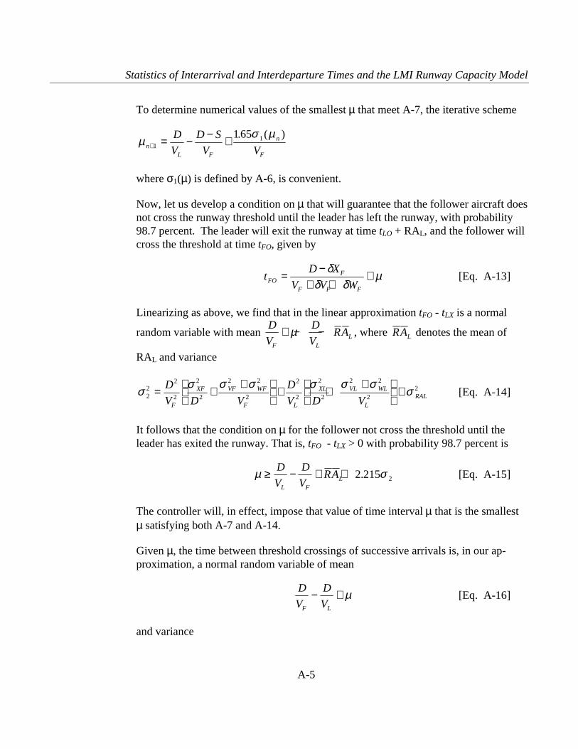
Statistics of Interarrival and Interdeparture Times and the LMI Runway Capacity Model
A-5
To determine numerical values of the smallest µ that meet A-7, the iterative scheme
µσ µ
nL F
n
F
D
V
D S
V V+ = − − +11165. ( )
where σ1(µ) is defined by A-6, is convenient.
Now, let us develop a condition on µ that will guarantee that the follower aircraft doesnot cross the runway threshold until the leader has left the runway, with probability98.7 percent. The leader will exit the runway at time tLO + RAL, and the follower willcross the threshold at time tFO, given by
tD X
V V WFOF
F F F
=−
+ ++
δδ δ
µ [Eq. A-13]
Linearizing as above, we find that in the linear approximation tFO - tLX is a normal
random variable with mean D
V
D
VRA
F LL+ − −µ , where RAL denotes the mean of
RAL and variance
σ σ σ σ σ σ σσ2
22
2
2
2
2 2
2
2
2
2
2
2 2
22= +
+
+ +
+
+D
V D V
D
V D VF
XF VF WF
F L
XL VL WL
LRAL [Eq. A-14]
It follows that the condition on µ for the follower not cross the threshold until theleader has exited the runway. That is, tFO - tLX > 0 with probability 98.7 percent is
µ σ≥ − + +D
V
D
VRA
L FL 2 215 2. [Eq. A-15]
The controller will, in effect, impose that value of time interval µ that is the smallestµ satisfying both A-7 and A-14.
Given µ, the time between threshold crossings of successive arrivals is, in our ap-proximation, a normal random variable of mean
D
V
D
VF L
− + µ [Eq. A-16]
and variance

A-6
σ σ σ σ σ σ σ32
2
2
2
2
2 2
2
2
2
2
2
2 2
2= ++
+ +
+
D
V D V
D
V D VF
XF VF WF
F L
XL VL WL
L
[Eq. A-17]
FOLLOWER VELOCITY < LEADER VELOCITY
When the follower’s approach speed is slower than the leader’s, in the controller-based view the controller will bring the follower onto the common path after theleader has advanced a distance S along it, as illustrated in Figure A-2.
In this case, the positions of the two aircraft as functions of time are again given by A-1 and A-2. The miles-in-trail requirement is now, that XL(µ) - XF(µ) ≥ S, with prob-ability at least 95 percent. As
X X X V V W XL F L L L L F( ) ( ) ( )µ µ δ δ δ µ δ− = + + + − [Eq. A-18]
is a normal random variable of mean VLµ and variance
σ µ σ σ σ σ42 2 2 2 2 2= + + +( )VL WL XF XL [Eq. A-19]
it follows that the condition that the miles-in-trail requirement is met, with 95 percentconfidence, is
Figure A-2. Time Phase of Arrivals when Follower Velocity < Leader Velocity
0 1 2 3 4 5 60
2
4
6
8
Time (minutes)
Threshold
S
| |µ
D

Statistics of Interarrival and Interdeparture Times and the LMI Runway Capacity Model
A-7
µ σ≥ +S
V VL L
165 4. [Eq. A-20]
Equation A-19 may be written as a single condition on µ using equation A-8 by re-placing equations A-9, A-10, and A-11 with the new definitions
AS
VL
≡
BV
VL WL
L
2 22 2
2165≡+
.σ σ
CV
XL XF
L
2 22 2
2165≡+
.σ σ
The condition that the single-occupant rule is met with 98.7 percent confidence isderived exactly as is that condition for VF ≥ VL (i.e., condition A-14). In the presentcase, too, the result is given by equation A-14. Also, in the present case, equations forthe mean and standard deviation of IAT, given µ, are given by A-15 and A-16.
ARRIVAL-DEPARTURE-ARRIVAL-DEPARTURE SEQUENCES
We can readily translate the results of the previous section to results for repeated A-Doperations by replacing RAL with RAL + RDD, where the subscript D denotes the in-tervening departure aircraft. This case is illustrated by Figure A-3.

A-8
It may be desirable to consider the effect of a communications lag c on the departure.If so, then RAL is replaced by RAL + c + RDD.
Statistics of Multiple Operations
At this point, we have expressions for the means and variances of normal randomvariables representing interarrival times for a variety of cases. Now we wish to usethese, to generate statistics of multiple arrivals, or multiple arrivals and departures, toproduce capacity curves for single runways and combinations of runways.
First, we consider the statistics of sequences of arrivals only. Statistics of the overallinterarrival time will be determined by the mix of aircraft using the runway, with theirindividual values of the aircraft parameters of Table A-1. Suppose three aircraft typesuse the runway, and the fraction of the aircraft of type i in the mix is pi. The previousresults give interarrival time for each pair as a normal random variable. Let the meanand standard deviation for aircraft type i following aircraft type j be µij and σij , re-spectively. Then the distribution function for overall interarrival time is
( )p t p p N tAAi j
i j ij ij= ΣΣ ( ; , )µ σ [Eq. A-21]
Figure A-3. Time Phase of Arrivals with Intervening Departure
0 1 2 3 4 5 6-6
-4
-2
0
2
Time (minutes)
| |RA RD|

Statistics of Interarrival and Interdeparture Times and the LMI Runway Capacity Model
A-9
where N(t; µ, σ) denotes the normal probability distribution function. Obviously, thedistribution of interarrival times is not normal. An example of an interarrival timedistribution of the type A-21 is shown in Figure A-4.
As Figure A-4 shows, the interarrival time distribution is not necessarily monomodal.
One can compute the mean and variance of the interarrival time distribution,A-21, straightforwardly: The results are
< >=t p pAAi j
i j ijΣΣ µ [Eq. A-22]
and
var( ) ( )t p p tAAi j
i j ij ij AA= + − < >ΣΣ σ µ2 2 2 [Eq. A-23]
In principle, one can compute exactly the distributions of total arrival times for A-A-A sequences of arbitrary length and find exact values for the number of arrivals thatcan, with assigned confidence, be accommodated in 1 hour. These calculations in-
Figure A-4. Interarrival Time (Distribution)
0.0
0.2
0.4
0.6
0.8
1.0
1.2
1.4
0.0 0.5 1.0 1.5 2.0 2.5 3.0 3.5 4.0 4.5
Minut es
Rel
ativ
e F
requ
ency

A-10
volve sums of many terms, however, and this motivates a search for useful approxi-mations.
Sums of normal random variables are normally distributed, and it is tempting to ap-proximate the distribution of sequences of many arrivals in such a way. An A-A-A...sequence with Jij cases of aircraft of type i following aircraft of type j has a normaldistribution whose parameters are easily computed. If one could choose the Jij so thatJij = pipjM, where M is the sum of the Jij , then the resulting normal distribution wouldbe a good approximation for the distribution of long arrival sequences. Unfortu-nately, for the aircraft mixes at some airports, some of the pi are only a few hun-dredths, so M would have to be several thousand for this approximation to beaccurate.
Nevertheless, because much of our work to this point has been approximate, it doesnot seem unreasonable to consider this “very large sequence”-limiting case. In thisapproximation, then, the time tM of M interarrival times has a normal distribution ofmean M<tAA> and variance
var( )t M p pMi j
i j ij= ΣΣ σ2 [Eq. A-24]
This result suggests approximating the distribution of interarrival time with a normaldistribution of mean <tAA> and variance v1 given by
v p pi j
i j ij12= ΣΣ σ [Eq. A-25]
It may be more appropriate to use the approximation v1 as an input for the variance ofinterarrival time in the FAA Airfield Capacity Model than the actual variance given inA-23. This is because that model appears to use the IAT variance in computing prop-erties of sequences of large numbers of operations.

Statistics of Interarrival and Interdeparture Times and the LMI Runway Capacity Model
A-11
We can use the approximation of A-25 to compute the number of arrivals that can beaccommodated in 1 hour with 95 percent confidence. That number M is determinedby the condition ( ) . ( )M t M vAA− < > + − ≤1 1 65 1 601 (only M-1 interarrival times
are required for M arrivals)13, which leads to the all-arrival capacity of a single run-way as M* = w2 + 1, where w is given by
wv
t
v
t tAA AA AA
= −< >
+< >
+
< >165
2
165
2
601 1
2. .
To compute the expected number of arrivals we use
M tAA= < >
60
RUNWAY CAPACITY CURVE
At this point, we have one point on the single-runway capacity curve, the one corre-sponding to all arrivals and no departures. We can generate others.
The distribution function of Figure A-4 suggests that there is a significant probabilityof interarrival times large enough to accommodate a departure. We can reckon thenumber of “free” departures (i.e., departures that can be accommodated in a stream of
Marrivals), in this way: The distribution of interarrival time is given by A-21). Weassume that departure ROT, arrival ROT, and communication delay are normal ran-dom variables of means <RD>, <RA>, and <c> and standard deviations σD, σA, and σc.Thus, the distribution of the difference t - RD - RA - c, where t is the IAT, is given by
13 This statement is accurate for any single hour considered in isolation; for a long run average, re-
place M-1 by M.

A-12
p t R R c
N R R c p p N
p p N R R c
A D
D A D A C i j ij ijji
i j ij D Aj
D ij A ci
( )
( , ) ( , )
( , )
− − −
= − < > − < > − < > + + ⊗
= − < > − < >− < > + + +
∑∑∑∑
σ σ σ µ σ
µ σ σ σ σ
2 2 2
2 2 2 2
[Eq. A-26]
where the symbol ⊗ denotes convolution14. Then the probability that t - RD - RA -c ispositive is given by
p p p C R R ci j
i j ij D A D ij A c+ = − − < > − < > − < > + + +1 0 2 2 2 2ΣΣ ( , , )µ σ σ σ σ
[Eq. A-27]
where C(t, µ,σ) is the normal cumulative probability function. This value is readily
computed. Then one may determine the number N of positive values of t-RD-RA-c to
be expected, in M draws, from the binomial distribution for probability p+.
Under IMC2 or IMC3 weather conditions, current FAA procedures require that de-partures be held if an arriving aircraft is within a certain distance of the runwaythreshold. (This distance is now 2 miles.) In our model, this has the effect of reduc-ing the time available for departing aircraft. Since the trailing arrival travels a dis-tance less than the full length of the common path, the uncertainties embodied in A-17 are also reduced.
The appropriate modification to A-16 is to reduce the IAT by DT
VF where DT is the
distance from threshold after which departures must be held. The variance in A-17reduced by
14 To account for variations in departure runway occupancy time, one may replace the single nor-
mal distribution of ROT with the distribution of departure ROT that would be found with K classes ofdeparting aircraft, each with its own normal distribution of departure ROT. That is,
q N Ri D i Di
K
( , )− < >∑ σ1
where qi denotes the fraction of departing aircraft that are of type i .

Statistics of Interarrival and Interdeparture Times and the LMI Runway Capacity Model
A-13
DT D DTV VF
VF WF
F
( )22
2 2
2
∗ − +
σ σ
A third point on the capacity curve, the point of equal numbers of arrivals and depar-tures, may be computed by considering sequences of repeated A-D pairs, as describedin the section above.
While the expressions for interarrival times and runway capacities developed aboveare somewhat lengthy, they are readily evaluated numerically.
Departures
Similar considerations lead to statistics of departures. The basic departure situation isshown in Figure A-5.
Figure A-5. Time Phase of Departures
0 1 2 3 4 50
1
2
3
4
5
6
Time (minutes)µ
S
Distance at which departures may turn

A-14
We model the trajectory of a departing aircraft by specifying its position, x(t), interms of the parameters VD and RD, in this way:
x t
V
Rt t R
V t V R t R
D
DD
D D D D
( ),
,=
< ≤
− ≥
1
20
1
2
2
This model approximates an actual takeoff roll and climb out by a trajectory withconstant acceleration from rest to departure speed VD, occurring in time RD, followedby continuing departure at constant speed VD.
We model controllers' actions on departures by the interdeparture time interval µ,which is the time interval between the start of the lead aircraft's takeoff roll to issuinga departure clearance to the following aircraft. (The following aircraft begins takeoffrole at time µ + c where c models the delay to move into position) We assume that,
in effect, controllers adjust µ to give specified confidence that miles-in-trail require-ments, and other separation requirements, are met.
Here again, the required control input varies, depending on whether the following air-craft is faster or slower than the lead aircraft. In the case of a faster follower, the con-straining condition is that the MIT requirement be met as the lead aircraft exits thesystem. At that time, the displacement of the lead aircraft is DD, the distance-to-turnon departure. The displacement of the following aircraft must not be greater than DD -SD, where SD is the minimum MIT spacing. After lengthy but straightforward steps,one finds that meeting this condition with 95 percent confidence imposes the condi-tion
( )µ ≥ + − −−
− +D
VR R
D S
Vc
VD
DLDL DF
D D
DF DF
12
165.var
on µ. The quantity var in the inequality just above is
( ) ( )var =D
VD
DL
+ − − −
+ +
++
12 4
2
2 22
22
2 2
2
22R R c
V
VD
V
VDL DF V W
DF
DLD
VL WL
DL
DFRDLDF F
µ σ σσ σ
σ
+ +14
2 2 2 2V VDF RDF DF Cσ σ
The inequality may be reduced to an equivalent, explicit condition on µ. For numeri-cal work, we find that iterative methods give the required values of µ conveniently.

Statistics of Interarrival and Interdeparture Times and the LMI Runway Capacity Model
A-15
When the follower departs more slowly than the leader, the MIT minima apply as thefollower lifts off, unless DD is sufficiently short that the leader can exit the systembefore the follower completes the takeoff roll. Applying the MIT minimum as thefollower lifts off leads to the condition
µ ≥ + −
− + +
R V
VR c
S
VDL DF
DLDF
D
DL212
1 165 1. var
where
( )var1 12 1
2
22 2
2
2
2= + + −+
+ −
µ
σ σσc R R
V
V
VDF DL
V WL
DL
DF
DLRDF
DL
+ ++
+
14
2 22 2
22σ
σ σσRDL DF
VDF WF
DLCR
V (inequality A)
Alternatively, the controller might impose a value of µ that caused the follower to liftoff just as the leader exited the system. That would lead to
µ σσ σ
σ σ≥ + − − + ++
+ +D
VR R c
D
V VD
DLDL DF RDF
D
DL
V WL
DLRDL C
DL12
16514
22
2
2 2
22 2.
(inequality B)
Controllers would impose the less restrictive of inequality A, or inequality B. Finally,the single-occupant rule must be respected, which leads to
µ σ σ≥ − + +R cDL RDL C2215 2 2. (inequality C)
For our model, when the follower is slower than the leader, we choose
µ = max (min(µA, µB), µC),
where µi is the lower bound on µ resulting from inequality i.
The PASCAL code for the LMI Runway Capacity Model follows.
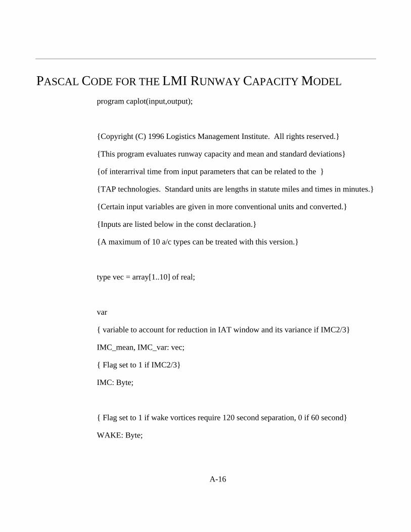
A-16
PASCAL CODE FOR THE LMI RUNWAY CAPACITY MODEL
program caplot(input,output);
{Copyright (C) 1996 Logistics Management Institute. All rights reserved.}
{This program evaluates runway capacity and mean and standard deviations}
{of interarrival time from input parameters that can be related to the }
{TAP technologies. Standard units are lengths in statute miles and times in minutes.}
{Certain input variables are given in more conventional units and converted.}
{Inputs are listed below in the const declaration.}
{A maximum of 10 a/c types can be treated with this version.}
type vec = array[1..10] of real;
var
{ variable to account for reduction in IAT window and its variance if IMC2/3}
IMC_mean, IMC_var: vec;
{ Flag set to 1 if IMC2/3}
IMC: Byte;
{ Flag set to 1 if wake vortices require 120 second separation, 0 if 60 second}
WAKE: Byte;

Statistics of Interarrival and Interdeparture Times and the LMI Runway Capacity Model
A-17
{Miles-in-trail for arrivals, in miles: sn[i,j] is MIT for i behind j, in}
{nautical miles.}
sn:array[1..10,1..10] of real;
{aircraft mix:}
p:vec;
{approach speeds, and s.d. of approach speeds, in knots:}
vk:vec;
sdvk:vec;
{Position uncertainties, nautical miles:}
sdxn:vec;
{Length of common approach path, nautical miles:}
dn:real;
{Standard deviation of wind, knots:}
sdwk:real;
{Arrival ROT and s.d. of arrival ROT, minutes:}
RA:vec;
sdra:vec;

A-18
{Departure ROT and s.d. of departure ROT, minutes:}
RD:vec;
sdrd:vec;
{Departure speeds and s.d. of departure speeds, in knots:}
vdk:vec;
sdvdk:vec;
{Minimum distance before turn on departure, nautical miles:}
ddn:real;
{Miles-in-trail for departures: assumed same as miles-in -trail for arrivals.}
{Communication delay mean and standard deviation, minutes:}
cbar:real;
sdc:real;
{Number of a/c types:}
nc:integer;
{End of input data}

Statistics of Interarrival and Interdeparture Times and the LMI Runway Capacity Model
A-19
var
v,sdv,vd,sdvd,sdx:vec;
s:array[1..10,1..10] of real;
xmu:array[0..1] of real;
d, dd, sdw:real;
i,j,k,l,f,m,nn:integer;
mu1, mu2,x0,x,rvf,rvl,s1,s2,mu,iat,sdiat,taa,sdtaa,rdbar,ssdrd,tdd,v1,v2,v3,v4,v5:real;
pclear,qclear:real;
{times[i,j,1] is mean iat, and times[i,j,2] is sdiat,for i behind j}
times:array[1..10,1..10,1..2] of real;
{Amax is max arrival rate, arrivals only; AD is max A=D rate; Dmax is }
{max departure rate; jmax is max departures in amax arrivals.}
abar: real;
amax,ad,dmax:real;
jmax:integer;
{gov[i,j] identifies controlling constraint - MIT or ROT - for i behind j.}
gg:string[3];

A-20
ts:char;
gov:array[1..10,1..10] of string[3];
ifl,ofl:text;
lab:string[80];
{Now load function cum(x,mu,sd:real):real, that returns cdf for normal }
{distribution at argument x, mean mu, standard deviation sd.}
{$i c:\tap\qm\cumf.pas}
function bf(x:real):real;
var
t,vv,s, df:real;
begin {bf is difference between 95% conf of dep and cur prob using sep x}
t:=1; {t = probability starting with 1}
if IMC = 1 then df:= d-2 else df:= d;
for k:=1 to nc do
begin
s:=sqrt(df*df/v[f]/v[f]*(sdx[f]*sdx[f]/df/df+rvf)
+d*d/v[l]/v[l]*(sdx[l]*sdx[l]/d/d+rvl)
+sdra[l]*sdra[l]+sdrd[k]*sdrd[k]+sdc*sdc);
vv:=-d/v[l]+df/v[f]-ra[l]-cbar-rd[k]+x;
t:=t-p[k]*cum(0,vv,s)

Statistics of Interarrival and Interdeparture Times and the LMI Runway Capacity Model
A-21
end;
{ Use 90% confidence on meeting slot width }
bf:=t-0.9 {find value of x that will make bf = 0 or t = 90}
end; {bf}
procedure aad;
var z:real;
begin {aad}
xmu[0]:=0;xmu[1]:=5;
if bf(xmu[0])*bf(xmu[1]) < 0
then
while (abs(xmu[0]-xmu[1]) > 1.e-5) do
begin
z:=0.5*(xmu[0]+xmu[1]);
if (bf(xmu[0])*bf(z) < 0)
then
xmu[1]:=z
else
xmu[0]:=z
end
else
writeln(f,l,k,' Zero not bracketed');

A-22
mu2:=z;
end; {AAD}
procedure gainer;
var
r,sd,z:real;
begin {gainer}
{The MIT mu value is determined by iteration:}
x:=d/v[l]-(d-s[f,l])/v[f];x0:=1000;
while(abs((x-x0)/x)>=1.e-6)do
begin
x0:=x;
s1:=d*d*v[f]*v[f]/v[l]/v[l]*(rvf+sdx[l]*sdx[l]/d/d+rvl);
s1:=s1+x0*x0*v[f]*v[f]*rvf+sdx[f]*sdx[f];
x:=d/v[l]-(d-s[f,l])/v[f]+1.65*sqrt(s1)/v[f]
end;
mu1:=x;
{Now make the mu for the single-occupancy rule condition:}
if (ts = 'A')
then

Statistics of Interarrival and Interdeparture Times and the LMI Runway Capacity Model
A-23
begin
s2:=d*d/v[f]/v[f]*(sdx[f]*sdx[f]/d/d+rvf)
+d*d/v[l]/v[l]*(sdx[l]*sdx[l]/d/d+rvl)
+sdra[l]*sdra[l];
mu2:=d/v[l]-d/v[f]+ra[l]+2.215*sqrt(s2)
end
else
aad;
if(mu1 >=mu2)then mu:=mu1 else mu:=mu2;
if(mu1 >= mu2) then gg:='MIT' else gg:= 'ROT';
iat:=d/v[f]-d/v[l]+mu;
sdiat:=sqrt(d*d/v[f]/v[f]*(sdx[f]*sdx[f]/d/d+rvf)+d*d/v[l]/v[l]*(sdx[l]*sdx[l]/d/d+rvl));
end; {gainer}
procedure looser;
var
r,sd:real;
begin {looser}

A-24
{Here,too, we stabilize the first mu by iteration:}
x:=s[f,l]/v[f];x0:=1000;
while (abs((x-x0)/x)>1.e-6)do
begin
x0:=x;
x:=s[f,l]/v[l]+1.65*sqrt(x0*x0*rvl+(sdx[f]*sdx[f]+sdx[l]*sdx[l])/v[l]/v[l]);
end;
mu1:=x;
{Now make the mu for the single-occupancy rule condition:}
if (ts = 'A')
then
begin
s2:=d*d/v[f]/v[f]*(sdx[f]*sdx[f]/d/d+rvf)
+d*d/v[l]/v[l]*(sdx[l]*sdx[l]/d/d+rvl)
+sdra[l]*sdra[l];
mu2:=d/v[l]-d/v[f]+ra[l]+2.215*sqrt(s2)
end
else
aad;
if(mu1 >= mu2) then mu:=mu1 else mu:=mu2;

Statistics of Interarrival and Interdeparture Times and the LMI Runway Capacity Model
A-25
if(mu1 >= mu2) then gg:='MIT' else gg:='ROT';
iat:=d/v[f]-d/v[l]+mu;
sdiat:=sqrt(d*d/v[f]/v[f]*(sdx[f]*sdx[f]/d/d+rvf)+d*d/v[l]/v[l]*(sdx[l]*sdx[l]/d/d+rvl));
end; {looser}
procedure dgainer;
var
mu1,x,x0:real;
begin {dgainer}
{Must obey single-occupant rule with 98.7% confidence. This => one
{constraint on idt. We tentatively assign idt this value:}
mu:=rd[l]-cbar+2.215*sqrt(sqr(sdrd[l])+sqr(sdc));
{Iterate to determine mu from MIT constraint:}
x:=dd/vd[l]+0.5*(rd[l]-rd[f])-(dd-s[f,l])/vd[f] -cbar;x0:=1000;
while(abs((x-x0)/x0)>1.e-6) do
begin
x0:=x;
x:=dd/vd[l]+0.5*(rd[l]-rd[f])-(dd-s[f,l])/vd[f] -cbar;
x:=x+1.65*sqrt((dd/vd[l]+0.5*(rd[l]-rd[f])-x0-cbar)*(dd/vd[l]+0.5*(rd[l]-rd[f])-x0-cbar)*rvf

A-26
+dd*dd/vd[l]/vd[l]*rvl
+0.25*(sdrd[l]*sdrd[l]+sdrd[f]*sdrd[f])+sqr(sdc))
end;
if (mu<x) then mu:=x;
{Now store idt in times[f,l,1]:}
times[f,l,1]:=mu+cbar;
end; {dgainer}
procedure dlooser;
var
mua,mub,muc,mu:real;
begin {dlooser}
{Must obey single-occupant rule with 98.7% confidence. This => one}
{constraint on idt. We assign muc this value:}
muc:=rd[l]-cbar+2.215*sqrt(sqr(sdrd[l])+sqr(sdc));

Statistics of Interarrival and Interdeparture Times and the LMI Runway Capacity Model
A-27
{Iterate to determine mu from MIT constraint:}
x:=0.5*rd[l]+0.5*vd[f]/vd[l]*rd[f]-rd[f]+s[f,l]/vd[l]-cbar;x0:=1000;
while(abs((x-x0)/x0)>1.e-6) do
begin
x0:=x;
x:=0.5*rd[l]+0.5*vd[f]/vd[l]*rd[f]-rd[f]+s[f,l]/vd[l]-cbar;
x:=x+1.65*sqrt((rd[f]-0.5*rd[l]+x+cbar)*(rd[f]-0.5*rd[l]+x+cbar)*rvl
+sdrd[f]*sdrd[f]*(1-0.5*vd[f]/vd[l])*(1-0.5*vd[f]/vd[l])
+0.25*(sdrd[l]*sdrd[l]+rd[f]*rd[f]*vd[f]*vd[f]/vd[l]/vd[l]*rvf)
+ sdc*sdc)
end;
mua:=x;
{Assign mub to "early turn" constraint:}
mub:= dd/vd[l]+0.5*rd[l]-rd[f]-cbar
+1.65*sqrt(sdrd[f]*sdrd[f]+dd*dd/vd[l]/vd[l]*rvl+0.25*sdrd[l]*sdrd[l]+sdc*sdc);
{Now assign idt to max of (min(mua, mub), muc)}

A-28
if mua<mub then mu:=mua else mu:=mub;
if muc> mu then mu:=muc;
times[f,l,1]:=mu+cbar;
end; {dlooser}
procedure dequal;
var
tmp,idt:real;
begin {dequal}
{Here, when climb-out speeds are equal, we check both the "gainer" and}
{"looser" conditions, and make idt equal to the longest of these.}
dgainer;tmp:=times[f,l,1];
dlooser; if (times[f,l,1]> tmp) then idt:=times[f,l,1] else idt:=tmp;
times[f,l,1]:=idt
end; {dequal}
begin {main}
{Get input data and set up output file:}
lab:='c:\tap\qm\capdatk1.txt';
assign(ifl,lab);reset(ifl);
lab:='c:\tap\qm\capoutk1.txt';
assign(ofl,lab);rewrite(ofl);

Statistics of Interarrival and Interdeparture Times and the LMI Runway Capacity Model
A-29
read(ifl,nc);nc2:=nc*nc;
for i:=1 to nc do for j:=1 to nc do read(ifl,sn[i,j]);
for i:=1 to nc do read(ifl,p[i]);
for i:=1 to nc do read(ifl,vk[i]);
for i:=1 to nc do read(ifl,sdvk[i]);
for i:=1 to nc do read(ifl,sdxn[i]);
read(ifl,dn);
read(ifl,sdwk);
for i:=1 to nc do read(ifl,ra[i]);
for i:=1 to nc do read(ifl,sdra[i]);
for i:=1 to nc do read(ifl,rd[i]);
for i:=1 to nc do read(ifl,sdrd[i]);
for i:=1 to nc do read(ifl,vdk[i]);
for i:=1 to nc do read(ifl, sdvdk[i]);
read(ifl,ddn);
read(ifl,cbar);
read(ifl,sdc);
read(ifl, IMC);
read(ifl, WAKE);
{Generate properly dimensioned distances, velocities & S. D.'s of velocities:}

A-30
{The spreadsheet GUI for this code has ALL distances in nautical miles,}
{and ALL velocities in knots. The code uses statute miles as the standard}
{length, miles/minute as the standard speed unit, and minutes as the standard}
{time unit.}
{First, approach, departure speeds & s.d.'s of same, and pos'n uncertainties:}
for i:=1 to nc do
begin
v[i]:=vk[i]*6.08/5.28/60;
sdv[i]:=sdvk[i]*6.08/5.28/60;
vd[i]:=vdk[i]*6.08/5.28/60;
sdvd[i]:=sdvdk[i]*6.08/5.28/60;
sdx[i]:=sdxn[i]*6.08/5.28
end;
{Miles-in-Trail:}
for i:=1 to nc do for j := 1 to nc do s[i,j]:=6.08/5.28*sn[i,j];
{Common path:}
D := dn*6.08/5.28;
{Wind:}

Statistics of Interarrival and Interdeparture Times and the LMI Runway Capacity Model
A-31
sdw:= sdwk*6.08/5.28/60;
{Distance to departure turn:}
dd := 6.08/5.28*ddn;
{Make average departure ROT and sd of average ROT, for A-D calcs:}
rdbar:=0;for i:=1 to nc do rdbar:=rdbar+p[i]*rd[i];
ssdrd:=0;for i:=1 to nc do ssdrd:=ssdrd+p[i]*(sdrd[i]*sdrd[i]+rd[i]*rd[i]);
ssdrd:=ssdrd-rdbar*rdbar;
ssdrd:=sqrt(ssdrd);
{Now make IAT statistics for each leader,follower pair, for arrivals only:}
ts:='A';
for f:=1 to nc do for l:=1 to nc do
begin
rvf:=(sdv[f]*sdv[f]+sdw*sdw)/v[f]/v[f];
rvl:=(sdv[l]*sdv[l]+sdw*sdw)/v[l]/v[l];
if (v[f] >= v[l])
then
gainer
else
looser;
times[f,l,1]:=iat;times[f,l,2]:=sdiat;

A-32
gov[f,l]:=gg
end;
{Now make some overall averages}
taa:=0;sdtaa:=0;for i:=1 to nc do for j:=1 to nc do
begin
taa:=taa+p[i]*p[j]*times[i,j,1];
sdtaa:=sdtaa+p[i]*p[j]*(times[i,j,2]*times[i,j,2]+times[i,j,1]*times[i,j,1])
end;
abar:= 60/taa;
sdtaa:=sqrt(sdtaa-taa*taa);
amax:= abar;
nn:=trunc(amax);
{compute corrections ot IAT mean and variance when radar approaches}
{FAA regs require no departure if arrival within 2 miles of threshold}
if IMC=0 then for i:=1 to nc do begin IMC_mean[i]:= 0; IMC_var[i]:=0;end
else for i:=1 to nc do begin
IMC_mean[i]:= 2/v[i]; {reduction in usable iat window}
IMC_var[i]:= (4*(d-1)/v[i]/v[i])*((sdv[i]*sdv[i]+sdw*sdw)/v[i]/v[i]);
{variance reductions, too}
end;

Statistics of Interarrival and Interdeparture Times and the LMI Runway Capacity Model
A-33
{Now find probability of taa including a departure, on one draw:}
v1:=1;
{ Aggregate over all follower/leaders i/j and all departing classes l}
for i:=1 to nc do for j:=1 to nc do for l:=1 to nc do
v1:=v1
-p[i]*p[j]*p[l]*cum(0,times[i,j,1]-IMC_mean[i]-RA[j]-rd[l]-cbar,
sqrt(times[i,j,2]*times[i,j,2]-IMC_var[i]+sdra[j]*sdra[j]+sdrd[l]*sdrd[l]+sdc*sdc));
pclear:=v1;qclear:=1-pclear;
{Now find expected number of departures that can be integrated}
{in the number of arrivals that can be done in 1 hour }
v1:=exp(nn*ln(qclear));v2:=v1;j:=0;
while (v2 <= 0.5) do
begin
j:=j+1;
v1:=pclear/qclear*(nn-j+1)/j*v1;
v2:=v2+v1
end;
j:=j+1;
jmax:=j;
{Now consider adjusting arrival spacing so that a departure is always }

A-34
{accomodated between arrivals. This gives a third point on the capacity curve.}
ts:='B';
for f:=1 to nc do for l:=1 to nc do
begin
rvf:=(sdv[f]*sdv[f]+sdw*sdw)/v[f]/v[f];
rvl:=(sdv[l]*sdv[l]+sdw*sdw)/v[l]/v[l];
if (v[f] >= v[l])
then
gainer
else
looser;
times[f,l,1]:=iat;times[f,l,2]:=sdiat;
gov[f,l]:=gg
end;
{Now make some overall averages}
taa:=0;sdtaa:=0;for i:=1 to nc do for j:=1 to nc do
begin
taa:=taa+p[i]*p[j]*times[i,j,1];
sdtaa:=sdtaa+p[i]*p[j]*(times[i,j,2]*times[i,j,2]+times[i,j,1]*times[i,j,1])
end;
abar:= 60/taa;
sdtaa:=sqrt(sdtaa-taa*taa);

Statistics of Interarrival and Interdeparture Times and the LMI Runway Capacity Model
A-35
ad:= abar;
{Now deal with departures. First, develop departure capacity for D-D-D...}
for f:=1 to nc do for l:=1 to nc do
begin
rvf:=(sdvd[f]*sdvd[f]+sdw*sdw)/vd[f]/vd[f];
rvl:=(sdvd[l]*sdvd[l]+sdw*sdw)/vd[l]/vd[l];
if (vd[f] > vd[l])
then
dgainer
else
if(vd[f] < vd[l])
then
dlooser
else
dequal;
{An FAA reg requires 1 minute between departure clearances, }
{ so min idt is 1.0 }
if times[f,l,1] < 1 then times[f,l,1]:= 1;
{ When wake vorticies are present, must wait for 2 minutes after heavy/757 }
if (WAKE = 1) and (l>=4) and (times[f,l,1]<2+cbar) then times[f,l,1]:= 2+cbar;
end; { loop for D-D-D ..... }

A-36
{Now compute average idt:}
tdd:=0;for i:=1 to nc do for j:=1 to nc do tdd:=tdd+p[i]*p[j]*times[i,j,1];
dmax:=trunc(60/tdd);
v1:=0;v2:=jmax;
writeln(ofl,v1,' ',dmax);
writeln(ofl,ad,' ',ad);
writeln(ofl,amax,' ',v2);
writeln(ofl,amax,v1);
close(ofl)
end.