Estimating the Effects of Friendship Networks on Health Behaviors of Adolescents∗

Jason M. Fletcher Yale University

Stephen L. Ross

University of Connecticut

This Draft: March 3, 2011

Abstract Researchers typically examine peer effects by defining the peer group broadly (all classmates, schoolmates, neighbors) because of the lack of friendship information in many data sources as well as to enable the use of plausibly exogenous variation in peer group composition across cohorts in the same school. This paper estimates the effects of friend’s health behaviors on own health behaviors for adolescents. A causal effect of friend’s health behaviors is identified by comparing similar individuals who have the same friendship opportunities because they attend the same school and make the same friendship choices, under the assumption that the friendship choice reveals information about an individual’s unobservables. We combine this identification strategy with a cross-cohort, within school design so that the model is identified based on across grade differences in the clustering of health behaviors within specific friendship options. This strategy allows us to separate the effect of friends behavior on own behavior from the effect of friends observables attributes on behavior, a key aspect of the reflection problem. We use a partial equilibrium model of friendship formation in order to derive the conditions under which our identification strategy will provide consistent estimates, and the key assumption required for our strategy to be feasible is supported by the empirical patterns of across cohort variation that we observe in our data. Our results suggest that friendship network effects are important in determining adolescent tobacco and alcohol use, but are over-estimated in specifications that do not fully take into account the endogeneity of friendship selection by 15-25%.

∗ We received valuable comments from numerous seminar participants at Baylor University, Cornell University, Lafayette College, Lehigh University, Texas A&M, University of California-Santa Barbara, University of Texas-Austin, Yale University, Population Association of American Conference, and the Second Annual Economics of Risky Behaviors (AMERB) conference. We thank Michael Anderson, Tao Chen, Don Kenkel, Anna Mueller, Bruce Sacerdote, Rusty Tchernis and Gautam Tripathi for specific comments that improved the paper. This research uses data from Add Health, a program project designed by J. Richard Udry, Peter S. Bearman, and Kathleen Mullan Harris, and funded by a grant P01-HD31921 from the National Institute of Child Health and Human Development, with cooperative funding from 17 other agencies. Special acknowledgment is due Ronald R. Rindfuss and Barbara Entwisle for assistance in the original design. Persons interested in obtaining data files from Add Health should contact Add Health, Carolina Population Center, 123 W. Franklin Street, Chapel Hill, NC 27516-2524 (addhealth@unc.edu).

Introduction

Individuals in modern societies are socially connected in a multitude of ways. For

example, the social networking website Facebook.com has increased its membership by 100

million users during 2009, and now there are over 500 million users worldwide. Individuals use

their social networks to receive and send information as well as establish, update, and enforce

social norms of behavior. Both information acquisition as well as the impacts of social norms

within social networks could have large effects on the health behaviors of individuals,

particularly adolescents, who are particularly responsive to peer pressure (Brown et al. 1997).

This heightening of peer influence also takes place during the developmental stage when many

of the most costly health outcomes and behaviors are initiated. Our analysis will use detailed

information on individual’s health related behaviors and friendship networks from the National

Longitudinal Study of Adolescent Health (Add Health) to examine the role of social interactions

in these behaviors.

Many studies of social interactions find evidence of clustering of outcomes or behaviors

above and beyond the clustering that might have been expected based on individuals’

observables, including studies of crime (Glaeser, Sacerdote and Scheinkman 1996), employment

(Topa 1999, Bayer, Ross, and Topa 2008), welfare usage (Bertrand, Luttmer, and Mullainathan

2000), pre-natal care (Aizer and Currie 2004), and youth health behaviors (Weinberg 2008). We

also observe unexpectedly high levels of clustering on health behavior within grades of students

at the same school in our data. Specifically, if we look within schools, very little variation

remains across grades in student composition in terms of racial or socio-economic variables, but

we observe substantial across grade variation in health behaviors for student populations that are

nearly identical. The purpose of this paper is to determine whether the within friendship

clustering of health behaviors that lies underneath the clustering in specific grades is consistent

with the influence of friendship networks.

Our test for whether the social interactions between friends influences health behavior is

built on the idea that individuals who make the same friendship choices are likely to be more

similar overall than might be indicated by their observables. Specifically, we examine a partial

equilibrium model of friendship formation and use the model to illustrate the effect of controlling

for fixed effects associated with clusters of observationally equivalent individuals who face the

same friendship opportunity set and make the same friendship choices. We show that if

individual students face a shock in terms of exposure to health behaviors, then as the number of

friends becomes large the unobservables of individuals in the same friendship choice cluster will

be identical and so a cluster fixed effect will act as a non-parametric control function for

unobservable attributes that influence friendship formation and might affect health behaviors.1 In

future versions of the paper, we intend to demonstrate the properties of this identification

strategy in the case of a small number of friends using monte carlo simulations.

In order to develop our empirical model of health behavior, we will rely on several

empirical features of adolescent friendship networks. First, a large literature suggests that

individuals exhibit strong racial, gender, and age preferences when choosing their friends—likes

choose likes (Mayer and Puller 2008, Weinberg 2008). Second, data from the Add Health

suggests that most friendships occur within grades, which is important for our use of cross-

cohort variation in our identification strategy. Finally, as discussed above, individual grades

within schools are quite homogenous over racial and socio-economic composition. Specifically,

we will estimate models of youth drinking and smoking in high school that control for the share

of same sex-same school-same grade friends who exhibit this behavior and fixed effects based on

clusters of individuals who have the same race, ethnicity, and maternal educational attainment

(individual observables), same school (same friendship opportunity set over observables), and

same number of friends overall and for each racial and maternal education subgroup (same

friendship choices). In our preferred specification, we will randomly choose one individual from

each grade per cluster so that the model estimates are explicitly identified based on variation

across cohorts within a school.

This approach is similar to earlier analyses by Dale and Krueger (2002) and Fu and Ross

(2010) who use fixed effects for individuals who are equivalent on key attributes and then have

the same outcome or make the same choice as a reduced form control in order to minimize bias

from unobservables. However, our analysis has the advantage over these earlier studies because

the identification strategy contains a clear source of exogenous variation that can create cluster-

associated social interactions, namely differences in exposure to health behaviors associated with

belonging to a particular cohort or grade of students. Further, our friendship formation model

demonstrates the importance of having such a source of exogenous variation for identification.

1 Later in the paper, we will demonstrate that these fixed effects satisfy Blundell and Dias’s (2009) definition of a control function under these assumptions.

This strategy can be illustrated by the following thought exercise: consider a 9th grader

and 10th grader who attend the same high school. As we show in detail below, these students face

very similar friendship opportunities with respect to racial, gender, and socioeconomic

composition of their same-grade classmates, and yet there is substantial clustering of health

behaviors into specific cohorts within schools. Thus, if we compare two students who choose

similar “types” of friends based on race, maternal education, and other demographic

characteristics, there will exist substantial differences in health behaviors between the across

cohort friendship opportunities, and those differences in friends’ health behaviors is arguably

quasi-random. The key is that the age difference between the 9th grader and the 10th grader (who

attend the same high school and have the same preferences for “types” of friends) has effectively

randomized these two students into their actual friendship network.

As discussed above, under relatively straightforward assumptions concerning friendship

formation, the inclusion of fixed effects for friendship choices provides a control function as the

number of friends becomes large and will yield consistent estimates of the spillover effects of

friend’s behavior. Further, we expect that our on-going simulations will demonstrate that even

when the number of friendships is reasonably small (two to five) the reduction in bias can be

substantial if friend choices are matched on multiple attributes. Most significantly, these

assumptions allow us to separate the influence on individual behavior of friend’s behaviors from

the influence of the observable attributes of those friends (the reflection problem) because those

comparisons are made between individuals who have observationally equivalent sets of friends.

We find evidence that this strategy produces smaller “network effect” estimates than

more standard models; however we still find robust evidence of network effects on smoking and

drinking behavior of adolescents. Further, we find that peer health behaviors are statistically

insignificant predictors of predetermined student or family attributes and the estimated

coefficients in these models are much smaller than our estimates of the effect on health

behaviors.

Background Literature

A large body of research across multiple disciplines has shown very strong correlations in

health behaviors for individuals who are socially connected. One reason there has been so much

research and policy interest in exploring how networks affect health behaviors and outcomes is

the potentially large set of health interventions and policies that could be proposed to leverage

social influences on health behaviors. While the promise of using social networks to affect health

is compelling, so too are the empirical issues inherent in detecting causal effects of social

networks using observational data.

Four difficulties with estimating the causal effects of social networks on health are

particularly important (Manski 1993). First, individuals self-select into their social network;

smokers befriend smokers. Second, individuals in the same social network are simultaneously

affected by their shared environment; common exposure to a smoking ban likely reduces tobacco

use among all members of a social network. Third, it is difficult to separate the influence of an

individual’s behavior and an individual’s attributes in determining the health behaviors of his or

her friend. Fourth, social influences are likely reciprocal, which leads to simultaneity bias.

Unfortunately, failure to overcome these empirical difficulties casts considerable doubt on the

current knowledge base linking the health behaviors among individuals in the same social

network. Each of these biases can lead a researcher to incorrectly infer that social networks have

a causal influence on behavior. Thus, policies intended to utilize social networks to enhance

interventions to reduce unhealthy behaviors could be unable to affect change if social networks

do not actually have causal effects. Providing evidence of the causal mechanisms and the likely

effects of policies is essential to be able to properly leverage social network effects on health

behaviors.

There have been two directions that researchers have taken in estimating peer effects on

health behaviors: [1] focus on broadly defined peer groups, such as all classmates in a school, in

order to either (a) exploit cross-cohort population variation2 in classmate composition (Bifulco et

al. 2011, Fletcher 2010, 2008, Trogdon et al. 2008, Lundburg 2006, Clark and Loheac 2007)

and/or (b) use instrumental variable strategies (Powell et al. 2005, Gaviria and Raphael 20013) or

[2] focus on narrowly defined peer groups, such as nominated friends, where the issues with

endogeneity are thornier and the estimates are likely less credible (Troddon et al. 2008,

Christakis and Fowler 2007, 2008, Renna et al. 2008). In this paper, we seek to combine the

more credible research designs from the first literature with the more credible peer group

definitions of the second literature.

2 See also the similar literature estimating peer effects in education outcomes (Hoxby 2000, Lavy and Schlosser 2008, Hanushek et al. 2003) 3 Instruments used in these analyses are often questionable, such as census poverty measures. Fletcher (2010) provides suggestive evidence that these instruments are invalid and proposes alternatives. Trodgon et al. (2008) and Fletcher (2010) use a combination of fixed effects and instruments.

Since we focus on friendship networks as the definition of peer group in this paper, it is

necessary to outline what other researchers have done previously and how our strategy adds to

the literature in this area. There have been recent examinations of the effects of social networks

on obesity and smoking in the medical literature (Christakis and Fowler 2007, 2008), where

“friends” are measured by the names respondents provide as potential contact sources for future

survey waves. In order to control for endogeneity of friendships, Christakis and Fowler assume

that including lags of the outcome for both the respondent and his/her friend is sufficient, and

further they do not control for common environmental factors. Cohen-Cole and Fletcher (2008a)

show that adding controls for environmental factors eliminates any detectable social network

effects for obesity, and Cohen-Cole and Fletcher (2008b) show more generally that these

parsimonious models will produce social network effects even in outcomes where none are

expected to exist, such as for height.

Renna et al. (2008) and Trodgon et al. (2008) also focus on estimating social contagion in

obesity and control for endogeneity of friendship in part by using school fixed effects. However,

since substantial friendship sorting occurs within schools, school fixed effects likely do not

provide a full solution to the endogeneity of friend selection, unless students select friends

randomly within schools. In fact, our estimates of the influence of friends behavior using school

fixed effects are notably larger than estimates using friendship cluster fixed effects suggesting

that school fixed effects may not be sufficient to control for endogeneity. In addition, Renna et

al. (2008) and Trodgon et al. (2008) use instruments for friends’ weight, including friends’

parents’ obesity. Trodgon et al. also uses friends’ birth weight. It is unclear whether these

instruments are adequate, though, as they are observable or correlated with observables at the

time of friendship selection.

Calvó-Armengol et al. (in press) and Patachini and Zenou (2010) have extended the

literature by using a network fixed effects approach in their examination of peer effect in

education outcomes. Adolescents are assumed to choose among mutually exclusive networks of

friends. Within these networks, their best friends (based on friendship nominations) are used as

the peer exposure and their model of behavior controls for network fixed effects. The maintained

assumption with this approach is that adolescents endogenously choose a friendship group, but

within that group, actual “best friends” are random, an assumption that is verified for

observables. Patachini and Zenou (2010) also use the outcomes of friends’ friends (once

removed in the network) as instruments.

All of these studies rely on information about the individual and their friends in order to

identify the effect of friend’s behavior. Whether identification is based on controlling for lagged

outcomes, instrumenting for friends attributes or controlling for network fixed effects, all of

these studies use variation across individuals who are in the same social environment and so

reasonably may have contributed to that variation through their own choices. In the next section,

we develop a simple model of friendship formation and demonstrate circumstances under which

consistent estimates of the effect of friends’ health behavior on own health behavior can be

uncovered, and show that identification requires an exogenous shock in exposure to potential

friends who exhibit certain health related behaviors. Following the literature on peer effects, we

propose that across cohort variation within schools can provide this exogenous variation in

exposure to health behaviors and demonstrate empirically that health behaviors vary

substantially more across cohorts than student attributes, like race or parental education,

evidence consistent with our identification strategy.

Identification Strategy

In this paper, we seek to estimate the causal effects of friends’ health behaviors by

overcoming the many empirical obstacles we outline above, including selection into networks,

unobserved determinants of behaviors, and the joint determination of outcomes within a network.

The intuition behind our approach is that we seek to form comparison groups based on

information in the data that describes the friendship options of students as well as the students’

choices of friends (given these options) following the premise that individuals who make similar

decisions or have similar outcomes when facing the same set of options likely are very similar on

both observable and unobservable attributes. The beginning of this section illustrates this

intuition, the next two subsections derive formal results, and in a future draft, the final subsection

will present Monte Carlo results to illustrate how our identification strategy works in practice.

We begin with a slight modification to the relatively straightforward linear-in-means

model of social interactions (Manski, 1993; Moffit, 2001; Brock and Durlauf, 2001) by

restricting social interactions to arise from a subset of individuals “friends” within a social

environment (or school s) and dividing the unobservable into two components: an unobservable

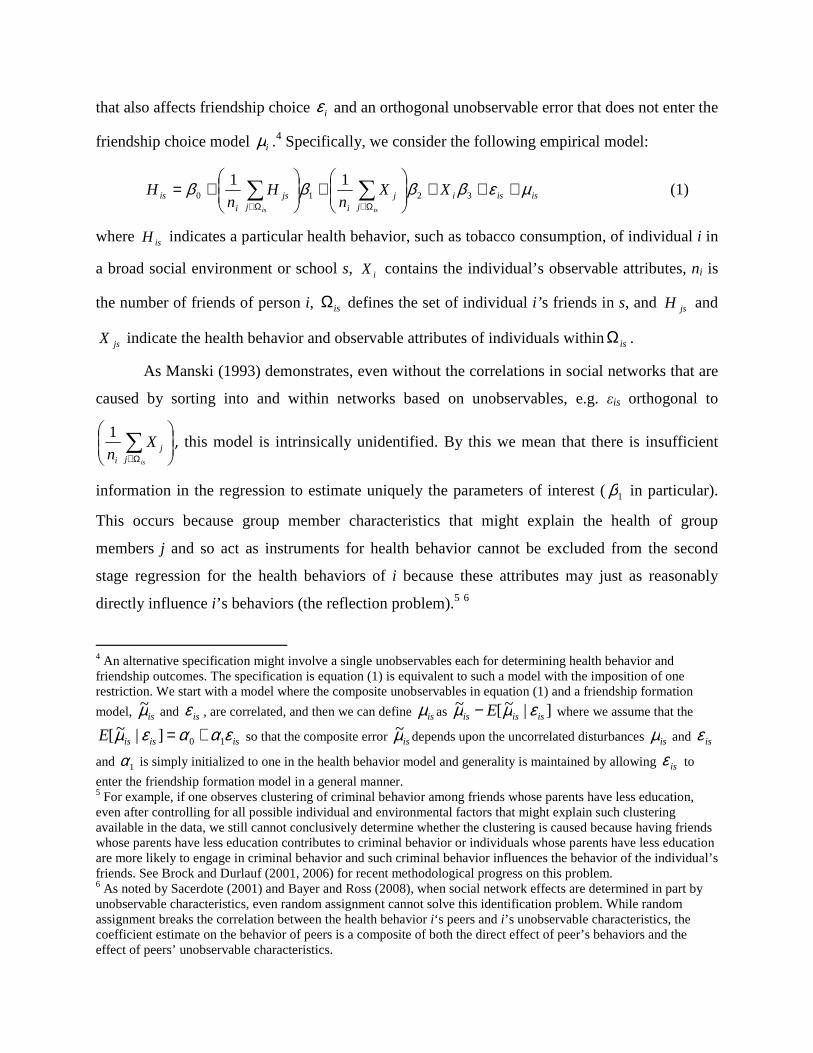
that also affects friendship choice iε and an orthogonal unobservable error that does not enter the

friendship choice model iµ .4 Specifically, we consider the following empirical model:

isisij

jij

jsi

is XXn

Hn

Hisis

µεββββ +++

+

+= ∑∑

Ω∈Ω∈3210

11 (1)

where isH indicates a particular health behavior, such as tobacco consumption, of individual i in

a broad social environment or school s, iX contains the individual’s observable attributes, ni is

the number of friends of person i, isΩ defines the set of individual i’ s friends in s, and jsH and

jsX indicate the health behavior and observable attributes of individuals within isΩ .

As Manski (1993) demonstrates, even without the correlations in social networks that are

caused by sorting into and within networks based on unobservables, e.g. εis orthogonal to

∑

Ω∈ isjj

i

Xn

1, this model is intrinsically unidentified. By this we mean that there is insufficient

information in the regression to estimate uniquely the parameters of interest (1β in particular).

This occurs because group member characteristics that might explain the health of group

members j and so act as instruments for health behavior cannot be excluded from the second

stage regression for the health behaviors of i because these attributes may just as reasonably

directly influence i ’s behaviors (the reflection problem).5 6

4 An alternative specification might involve a single unobservables each for determining health behavior and friendship outcomes. The specification is equation (1) is equivalent to such a model with the imposition of one restriction. We start with a model where the composite unobservables in equation (1) and a friendship formation

model, isµ~ and isε , are correlated, and then we can define isµ as ]|~[~isisis E εµµ − where we assume that the

isisisE εααεµ 10]|~[ += so that the composite error isµ~ depends upon the uncorrelated disturbances isµ and isε

and 1α is simply initialized to one in the health behavior model and generality is maintained by allowing isε to

enter the friendship formation model in a general manner. 5 For example, if one observes clustering of criminal behavior among friends whose parents have less education, even after controlling for all possible individual and environmental factors that might explain such clustering available in the data, we still cannot conclusively determine whether the clustering is caused because having friends whose parents have less education contributes to criminal behavior or individuals whose parents have less education are more likely to engage in criminal behavior and such criminal behavior influences the behavior of the individual’s friends. See Brock and Durlauf (2001, 2006) for recent methodological progress on this problem. 6 As noted by Sacerdote (2001) and Bayer and Ross (2008), when social network effects are determined in part by unobservable characteristics, even random assignment cannot solve this identification problem. While random assignment breaks the correlation between the health behavior i‘s peers and i’s unobservable characteristics, the coefficient estimate on the behavior of peers is a composite of both the direct effect of peer’s behaviors and the effect of peers’ unobservable characteristics.

Our identification strategy is to sort students into clusters c based on comparing similar

students who faced similar friendship options and made similar friendship choices. This sorting

is based on both observable (to the researcher) and unobservable characteristics. Following the

standard selection argument: if two individuals make similar choices and differ on observables,

then they are expected to differ on unobservables, as well (Heckman,1976). Similarly, if two

individuals are the same on observables and make similar choices, they are expected to be quite

similar on unobservables. Therefore, as argued by Dale and Krueger (2002) and Fu and Ross

(2010), the inclusion of fixed effects for such clusters should assure that we are comparing

students who are similar on both observables and unobservables, which breaks or weakens the

correlation between peers’ behaviors and a student’s unobservable characteristics. Further, since

all students in a cluster should have similar observable characteristics, the inclusion of the fixed

effect also captures the observables associated with the students’ peers while allowing the effect

of behavioral differences within a cluster to identify the effect of friend behavior on individual

behavior. This feature of the approach solves the empirical problem outlined above and isolates

the causal effect of student behaviors on the behavior of their friends from the effect of

observable friends’ attributes.

Specifically, define a cluster of individuals c in the same school who are observationally

equivalent on Xi and choose observationally equivalent friends based on Xj. This structure

implies that the individual and friendship group observables are the same within a cluster so that

the contribution of the variables that determine clusters to individual’s health behavior are

constant within cluster or

3232

11 ββββ kj

ji

ij

ji

XXn

XXn

ksis

+

=+

∑∑

Ω∈Ω∈ (2)

for all cki ∈, . Further, we assume that the models that define selection over friendships on

health behaviors and on observable attributes depend monotonically on the same observable

vector of attributes Xi and the same single index unobservable εis. This assumption is central to

our identification strategy. Without monotonicity, multiple values of the unobservable might be

consistent with the same friendship choices for observationally equivalent individuals. With

monotonicity, individuals who face the same friendship options based on the available social

network (s) and make the same choices should have similar values on the unobservable that

influences health behavior because if they differed substantially on the unobservable they would

likely have made different friendship choices.

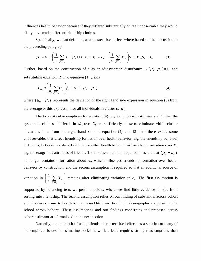
Specifically, we can define ρc as a cluster fixed effect where based on the discussion in

the preceeding paragraph

kskj

ji

isij

ji

c XXn

XXn

ksis

εβββεβββρ ++

+≈++

+≈ ∑∑

Ω∈Ω∈320320

11

(3)

Further, based on the construction of µ as an idiosyncratic disturbance, 0]|[ =icisE ρµ and

substituting equation (2) into equation (1) yields

)(

11 cisc

jj

iics

is

Hn

H µµρβ −++

≈ ∑

Ω∈ (4)

where )( cis µµ − represents the deviation of the right hand side expression in equation (3) from

the average of this expression for all individuals in cluster c, cµ .

The two critical assumptions for equation (4) to yield unbiased estimates are [1] that the

systematic choices of friends in isΩ over Xj are sufficiently dense to eliminate within cluster

deviations in ε from the right hand side of equation (4) and [2] that there exists some

unobservables that affect friendship formation over health behavior, e.g. the friendship behavior

of friends, but does not directly influence either health behavior or friendship formation over Xj,

e.g. the exogenous attributes of friends. The first assumption is required to assure that )( cis µµ −

no longer contains information about εis, which influences friendship formation over health

behavior by construction, and the second assumption is required so that an additional source of

variation in

∑

Ω∈ isjjs

i

Hn

1 remains after eliminating variation in εis. The first assumption is

supported by balancing tests we perform below, where we find little evidence of bias from

sorting into friendship. The second assumption relies on our finding of substantial across cohort

variation in exposure to health behaviors and little variation in the demographic composition of a

school across cohorts. These assumptions and our findings concerning the proposed across

cohort estimator are formalized in the next section.

Naturally, the approach of using friendship cluster fixed effects as a solution to many of

the empirical issues in estimating social network effects requires stronger assumptions than

random assignment or even traditional cohort based studies of peer effects, but this strategy

provides a significant payoff by potentially providing estimates of the effect of peer behaviors on

individual behaviors that are not contaminated by the direct influence of peer observable

characteristics, which is not accomplished by either random assignment or traditional across

cohort variation studies.7

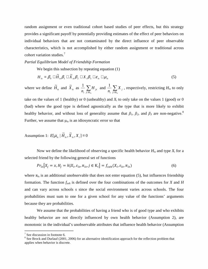
Partial Equilibrium Model of Friendship Formation

We begin this subsection by repeating equation (1)

isisiisisis XXHH µεββββ +++++= 3210

~~ (5)

where we define isH~

and isX~

as ∑Ω∈ isj

jsi

Hn

1 and ∑

Ω∈ isjj

i

Xn

1, respectively, restricting His to only

take on the values of 1 (healthy) or 0 (unhealthy) and Xi to only take on the values 1 (good) or 0

(bad) where the good type is defined agnostically as the type that is more likely to exhibit

healthy behavior, and without loss of generality assume that β1, β2, and β3 are non-negative.8

Further, we assume that µis is an idiosyncratic error so that

Assumption 1: 0],~

,~

|[ =iisisis XXHE µ

Now we define the likelihood of observing a specific health behavior His and type Xi for a

selected friend by the following general set of functions

, |, , , Κ , , (6) where πis is an additional unobservable that does not enter equation (5), but influences friendship

formation. The function fsxh is defined over the four combinations of the outcomes for X and H

and can vary across schools s since the social environment varies across schools. The four

probabilities must sum to one for a given school for any value of the functions’ arguments

because they are probabilities.

We assume that the probabilities of having a friend who is of good type and who exhibits

healthy behavior are not directly influenced by own health behavior (Assumption 2), are

monotonic in the individual’s unobservable attributes that influence health behavior (Assumption

7 See discussion in footnote 6. 8 See Brock and Durlauf (2001, 2006) for an alternative identification approach for the reflection problem that applies when behavior is discrete.

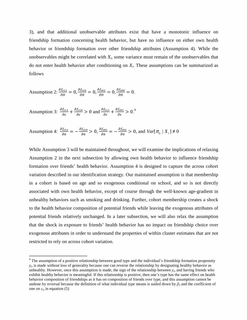
3), and that additional unobservable attributes exist that have a monotonic influence on

friendship formation concerning health behavior, but have no influence on either own health

behavior or friendship formation over other friendship attributes (Assumption 4). While the

unobservables might be correlated with Xi, some variance must remain of the unobservables that

do not enter health behavior after conditioning on Xi. These assumptions can be summarized as

follows

Assumption 2:

0,

0,

0,

0.

Assumption 3:

"#

"$ 0 and

"#

"$ 0.9

Assumption 4:

% &

%$ 0,

% &

%$ 0, and 0]|[ ≠iis XVar π

While Assumption 3 will be maintained throughout, we will examine the implications of relaxing

Assumption 2 in the next subsection by allowing own health behavior to influence friendship

formation over friends’ health behavior. Assumption 4 is designed to capture the across cohort

variation described in our identification strategy. Our maintained assumption is that membership

in a cohort is based on age and so exogenous conditional on school, and so is not directly

associated with own health behavior, except of course through the well-known age-gradient in

unhealthy behaviors such as smoking and drinking. Further, cohort membership creates a shock

to the health behavior composition of potential friends while leaving the exogenous attributes of

potential friends relatively unchanged. In a later subsection, we will also relax the assumption

that the shock in exposure to friends’ health behavior has no impact on friendship choice over

exogenous attributes in order to understand the properties of within cluster estimates that are not

restricted to rely on across cohort variation.

9 The assumption of a positive relationship between good type and the individual’s friendship formation propensity yis is made without loss of generality because one can reverse the relationship by designating healthy behavior as unhealthy. However, once this assumption is made, the sign of the relationship between yis and having friends who exhibit healthy behavior is meaningful. If this relationship is positive, then one’s type has the same effect on health behavior composition of friendships as it has on composition of friends over type, and this assumption cannot be undone by reversal because the definition of what individual type means is nailed down by β3 and the coefficient of one on εis in equation (5)

Based on equations (5) and (6), the probability of a friend exhibiting healthy behavior

depends upon the individual’s own observable and unobservable attributes that also directly

influence own health behavior, the resulting correlations will bias OLS estimates of β. In order to

characterize the bias from OLS estimation of equation (1) or (5), we write the expectation of

equation (5) as

],

~,

~|[

~~],

~,

~|[ 3210 iisisisitisisiisisis XXHEXXHXXHHE εββββ ++++=

(7)

and substitutethe linear projection of εis on the conditioning variables, 3210

~~ φφφφ iisis XXH +++

,10 into equation (5). This yields

)()(~

)(~

)(],~

,~

|[ 33221100 φβφβφβφβ +++++++= itisisiisjis XXHXXHHE (8)

Definition 1: Based on this linear projection, we define the bias in the estimated coefficient on

jH~

as

]],

~|

~[

~[

]],~

|~

[~

,[1

iisisis

iisisisis

XXHEHVar

XXHEHCov

−−

=εφ (9)11

Now having characterized the bias associated with the OLS estimate of our parameter of

interest, we define a cluster c as all students in a school are of the same type, have the same

number of friends, and make the same friendship choices over type.

Definition 2: A cluster c in school s is defined so that Xis = Xks, ni = nk and

∑∑Ω∈Ω∈

=ksis j

jskj

jsi

Xn

Xn

11 for all i and k in cluster c and their exist no individuals l outside of

cluster c where Xis = Xls, ni = nl and ∑∑Ω∈Ω∈

=lsis j

jslj

jsi

Xn

Xn

11.

10 This assumption is typically imposed when examining problems associated with errors-in-variables in a linear model, Even without imposing any linearity assumptions, one can interpret the estimates of β as the best linear predictor of H conditional on

isH~ ,

isX~ , Xi, and εis, and

1iφ is the relative bias in those estimates if one is unable to

condition on εis. 11 This arises from the standard omitted variables formula for a regressor that is orthogonal to all other regressors and othogonality is obtained using a conditioning argument where ' ()* # (+ # , can be rewritten as the following conditional regression ' ()* & -.*|/ # ()-.*|/ # (+ # ,.

In terms of the health behavior equation, a cluster fixed effect will take on the following

value

cciiscc XXH µεβββδ ++++= 321

~ (10)

where cH , cε and cµ are the means of isH~

, ε and µ within the cluster c.

After controlling for cluster fixed effects in equation (5), the health behavior model takes

the following form:

)()()~

( 1 ciscisccisis HHH µµεεδβ −+−++−= (11)

The bias associated with the estimated coefficient on )~

( cis HH − in this model is

)]

~[(

)]~

(,[

]]|)~

[()~

[(

]]|)~

[()~

(,[1

cis

ciscis

cciscis

ccisciscisc

HHVar

HHCov

HHEHHVar

HHEHHCov

−−−

=−−−

−−−−=

εεδ

δεεφ

(12)

Note that the expectation of the within cluster deviation in isH~

is zero because all observable

information that influences the composition of friends on health behavior, i.e. observed attributes

(Xi) or proxies for unobservable factors (isX~

for ) are the same for all individuals in a cluster.

Our first important result is that the bias in equation (12) limits to zero as the number of

friends becomes large.

Theorem 1. Under Assumptions 1 through 4 plus Definitions 1 and 2, the bias arising from

estimating the cluster fixed effects model in equation (12) limits to zero as ni becomes large for

all i in the sample.

Proof: First, the probability of a friend being of good type can be written as

1 )), , # )1, , 2, (13)

where the derivative of 2 is positive. As the number of friends becomes large,

lim6789X;<=

2 , (14)

because as the number of draws goes to infinity the empirical frequency must equal the

probability.

Since all individuals in cluster c have the same observable type and the same fraction

of good type friends, X;<=, equation (14) implies that

2 ,

2 , > for all cki ∈, (15)

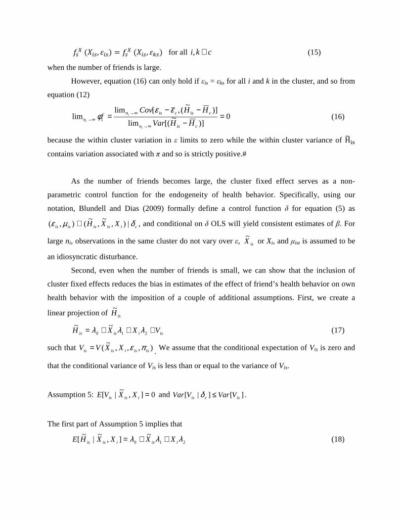
when the number of friends is large.

However, equation (16) can only hold if εis = εks for all i and k in the cluster, and so from

equation (12)

0)]

~[(lim

)]~

(,[limlim 1 =

−

−−=

∞→

∞→∞→

cisn

ciscisncn

HHVar

HHCov

i

i

i

εεφ (16)

because the within cluster variation in ε limits to zero while the within cluster variance of H;<=

contains variation associated with π and so is strictly positive.#

As the number of friends becomes large, the cluster fixed effect serves as a non-

parametric control function for the endogeneity of health behavior. Specifically, using our

notation, Blundell and Dias (2009) formally define a control function δ for equation (5) as

ciisisisis XXH δµε |),~

,~

(),( ⊥ , and conditional on δ OLS will yield consistent estimates of β. For

large ni, observations in the same cluster do not vary over ε, isX~

or Xi, and µist is assumed to be

an idiosyncratic disturbance.

Second, even when the number of friends is small, we can show that the inclusion of

cluster fixed effects reduces the bias in estimates of the effect of friend’s health behavior on own

health behavior with the imposition of a couple of additional assumptions. First, we create a

linear projection of isH~

isiisis VXXH +++= 210

~~ λλλ (17)

such that ),,,~

( isisiisis XXVV πε=. We assume that the conditional expectation of Vis is zero and

that the conditional variance of Vis is less than or equal to the variance of Vis.

Assumption 5: 0],~

|[ =iisis XXVE and ][]|[ iscis VVarVVar ≤δ .

The first part of Assumption 5 implies that

210

~],

~|

~[ λλλ iisiisis XXXXHE ++= (18)

This restriction is essentially is a law of large numbers style assumption where we assume that

the average of this residual is zero over repeated realizations of isH~

and isX~

for a given Xi. This

assumption would be standard if isX~

did not depend upon εis. While we cannot verify this

assumption in the data, we can examine whether this assumption holds in the monte carlo

assumptions under the substantially weaker assumption that Xi is uncorrelated with εis and πis.

The second half of Assumption 5 is something that can be theoretically violated in principle, but

in practice we expect that variances will decline after conditioning on additional information. We

can also directly verify this assumption in our data.

Theorem 2: Under Assumptions 1 through 5 plus Definitions 1 and 2, the bias arising from

estimating the cluster fixed effects model in equation (11) has the same sign and is smaller than

the bias that arises for the OLS model described in equation (5).

Proof: Using equation (17), the bias from the cohort fixed effect model in equation (12) reduces

to

][

],[

)]~

[(

)]~

(,[1

cis

ciscis

cis

ciscisc

VVVar

VVCov

HHVar

HHCov

−−−

=−

−−=

εεεεφ

(19)

where cV is the cohort mean of Vis.

The variance of the mean of a set of correlated variables is a well known expression

],|,[1

][1

][ ckiVVCovm

mVVar

mVVar ksis

i

iis

ic ∈

−−= = (20)

where mi is the number of individual in i’s cluster. Similarly,

],|,[1

][1

],[ ckiVVCovm

mVVar

mVVCov ksis

i

iis

icis ∈

−−= (21)

so that the denominator of equation (19) takes the form

( )],|,[][1

1][ ckiVVCovVVarm

VVVar ksisisi

cis ∈−

−=− (22)

Turning to the numerator of equation (19), the three relevant covariance terms are

],[ cis VCovε , ],[ cisVCov ε and ],[ cc VCovε , which take the following form as illustrated for

],|,[1

],[1

],[ ckiVCovm

mVCov

mVCov ksis

i

iisis

icis ∈

−−= εεε (23)

Using all three covariance terms,

( )],|,[],[1

1],[ ckiVCovVCovm

VVCov ksisisisi

ciscis ∈−

−=−− εεεε (24)

and Equation (19) can be rewritten using equations (22) and (24) as

( )( )],|,[][

],|,[],[1 ckiVVCovVVar

ckiVCovVCov

ksisis

ksisisisc

∈−∈−

=εεφ (25)

Next, using equations (17) and (18) the OLS bias in equation (9) reduces to

][

],[

]],~

|~

[~

[

]],~

|~

[~

,[1

is

isis

iisisis

iisisisis

VVar

VCov

XXHEHVar

XXHEHCov εεφ =−

−=

(26)

Note that the first terms in the numerator and denominator in equation (25) are the same as the

numerator and denominator in equation (26). Equation (25) will be smaller than equation (26) if

the relative or percentage reduction in the first numerator term caused by the second numerator

term in equation (25) is smaller than the equivalent reduction in the denominator or if

][

],|,[

],[

],|,[

is

ksis

isis

ksis

VVar

ckiVVCov

VCov

ckiVCov ∈>

∈ε

ε (27)12

Without additional loss of generality, we can create a linear projection of Vis on εis

isisis UV ++= 10 ξεξ (28)

where ),,,~

( isisiisis XXUU πε= and ],[ isis UCovε .

Further, ],|,[ ckiUCov ksis ∈ε and ],|,[ ckiUUCov ksis ∈

both also equal zero because the

all sources of a linear relationship between the sH '~

within cohort has been eliminated. Uks

depends on πks, but any linear dependence with εks and Xis has been eliminated from U through

the linear projections and selection into clusters does not depend upon or correlate with πis due to

Assumption 3 and so does not contribute to the covariances.

12 This condition holds regardless of the sign of the covariances. For example, if the covariances in the numerator of equation (27) are both negative, they imply an increase in both the numerator and denominator and the bias is reduced if the numerator in equation (26) increases by less. This requires that the right hand side of equation (27) be larger magntidue, which is then smaller in value because the terms of negative.

Using equation (28) and the above results, we can rewrite equation (27) as

][1

][

],|,[

][

],|,[

21

isis

ksis

is

ksis

UVarVar

ckiCov

Var

ckiCov

ξε

εεε

εε

+

∈>

∈ (29)

The variance of Uis is unambiguously positive because of the variation associated with πis so this

condition holds as long as ],|,[ ckiCov ksis ∈εε is positive.

From equation (7) and Assumption 1, we know that the probability of having good type

friends 2 increases monotonically with εis and so the expected value of isX

~ must also increase

monotonically with εis.13 Therefore, we can express the fraction of good type friends as a

monotonic function of εis and a stochastic variable of unknown form

@ A2, , B (30)

Since the two individuals in the same cluster have the same fraction of good type friends isX~

and

are of the same type themselves iX

A2, , B A

2, >, B> (31)

where νis is an idiosyncratic error term so that -., C/ 0.

The implicit function theorem and monotonicity assumption allows us to rewrite (31) as

A"D), B, A

2>, >, B> E AF>, , B, B> (32)

where A"D) is the partial inverse of A

2 with respect to the εis argument and is monotonically

increasing in the third argument, A2, for person k, and since > only enters the equation once

and is inside of two monotonic functions A G can be defined as a monotonic function of >. The

covariance can now be rewritten as

0],|),,,,(~[],|,[ >∈=∈ ckiXgCovckiCov ksksisiksksis ευυεεε (33)

which is unambiguously positive due to the monotonicity of AH.

In order to sign the cohort fixed effects bias in equation (25) relative to the OLS bias in

equation (26), we substitute equation (28) in the numerators of the bias expressions. For OLS,

the expression reduces to

)(][

][)( 1

11 ξεξφ sign

VVar

Varsignsign

is

is =

=

(34)

which takes the same sign as ξ1. For the cohort fixed effects model, 13 The following argument also holds for a monotonically decreasing function.

( )( ) )(

],|,[][

],|,[][)( 1

11 ξεεεξφ sign

ckiVVCovVVar

ckiCovVarsignsign

ksisis

ksisisc =

∈−∈−

= (35)

which will take the same sign as ξ1 if both the terms in the numerator and denominator are

unambiguously positive. The positive numerator and denominator hold due to Assumption 5

combined with the fact that a covariance of two related draws from a distribution cannot exceed

the variance of this distribution. Specifically,

],|,[]|[][ ckiVVCovVVarVVar ksiscisis ∈≥≥ δ (36)

#

Simultaneity of Health Behavior and Friendship Sorting Model

In this section, we extend the friendship formation function so that friendship formation

over health behavior depends upon one’s own health behaviors creating true simultaneity

between one’s own health choices and the selection of friends based on their health choices.

Specifically, we relax Assumption 1 so that own health behavior influences the likelihood of

having friends who exhibit a health behavior, but do not allow own health behavior to affect

friendship formation over the observable attributes. So

, |, , , , Κ , , , (36) with

Assumption 6:

&

$ 0 and

&

$ 0.

Therefore, the idiosyncratic error µis does not have a conditional expectation of zero because it

influences the health behavior of friends jH~

through one’s own health behavior, and the bias in

the coefficient on friend’s health behaviors contains a second term. Specifically,

],~

,~

|[~~

],~

,~

|[ 3210 iisisisisitisisiisisis XXHEXXHXXHHE µεββββ +++++= (37)

10

~],

~,

~|[ ϕϕµ isiisisis HXXHE += (38)

)(

)(~

)(~

)(],~

,~

|[

33

22111000

φβφβϕφβϕφβ

+

++++++++=

it

isisiisjis

X

XHXXHHE (39)

where using the expansion in equation (17) the new bias term may be expressed as

][

],[

]],~

|~

[~

[

]],~

|~

[~

,[1

is

isis

iisisis

iisisisis

VVar

VCov

XXHEHVar

XXHEHCov µµϕ =−

−= (40)

Definition 3: The reduced form effect of friend’s health behavior on own health behavior is

defined as (β1+φ1). This value includes both the direct effect of friend’s health behavior and the

additional multiplier effect because own health behavior influences friend’s health behavior.

Taking the expectation of the cluster fixed effects model in equation (11) yields

],~

|)[(

],~

|)[()~

(],~

|[ 1

cciscis

cciscisccisccisis

HHE

HHEHHHHHE

δµµδεεδβδ

−−

+−−++−=− (41)

The form of the bias in the estimated coefficient on )~

( cis HH − that is associated with the

expectation over )( cis εε − has been previously defined in equation (12). Again exploiting the

expansion in equation (17), the bias associated with the expectation over )( cis µµ − is

][

],[

]]|)~

[()~

[(

]]|)~

[()~

(,[1

cis

ciscis

cciscis

ccisciscisc

VVVar

VVCov

HHEHHVar

HHEHHCov

−−−

=−−−

−−−−=

µµδ

δµµϕ

(42)

Theorem 3. Under Assumptions 1 and 3 through 6 plus Definitions 1, 2 and 3, the cluster fixed

effects model estimate of the effect of friends’ health behavior limits to the reduced form

estimate (β1+φ1) as ni becomes large for all i in the sample.

Proof: By equation (39), the expectation of the estimate of the effect of friends’ health behavior

in the cluster fixed effects model is )( 111cc ϕφβ ++ , and Theorem 1 establishes that c

1φ limits to

zero with the number of friends.

Following the derivations in equations (20) through (25) except for µ instead of ε yields

( )( )],|,[][

],|,[],[1 ckiVVCovVVar

ckiVCovVCov

ksisis

ksisisisc

∈−∈−

=µµφ

(43)

However, membership in the cluster c only depends upon isX and isX~

and so provides no

information concerning the expectation of either isµ or isV since isµ is orthogonal to these

variables by assumption and isV is orthogonal by construction. Therefore the covariance terms

between i and k are zero,

11 ][

],[ ϕµϕ ==is

isisc

VVar

VCov (44)

and

11111111 )(lim)(lim ϕβϕφβϕφβ +=++=++ ∞→∞→c

ncc

n ii#

Generalizing the Shock to Friendship Composition

In this section, we relax Assumption (4) concerning the shock to friendship composition

over health behavior so that this shock affects friendship composition over both health behavior

and attributes. Assumption (2) is primarily supported by our across cohort identification strategy,

and may be violated in models that are identified by within cohort variation in friendship

choices. In that context, this extension is considered for two reasons: 1. To illustrate that

Assumption (4) is crucial for our identification strategy and 2. To illustrate the potential bias in

models that we estimate below that exploit within cohort variation.

One possible alternative is to redefine the set of functions that describe the likelihood of

observing a specific health behavior His and type Xi as

, |, , , Κ , ' # ( , (6) And replace assumptions (3) and (4) with

Assumption 7:

I#

I$ 0,

I#

I$ 0,

% &

%$ 0 and

% &

%$ 0

which retains our monotonicity assumption in the effect of attributes on friendship, but now over

a linear combination of εis and πis. As the number of friends becomes large,

lim6789X;<=

2 , # ( (45)

and

2 , # (

2 , > # (> for all cki ∈,

(46)

where c is defined based on constant and X;<= as in Definition 1. This implies that

# ( > # (> for all cki ∈,

(47)

Further, equation (47) implies that

& JK ( & LK (48)

where JK and LK are the cohort means of εis and πis.

Now as in Theorem 2, we expand Vis from equation (17) in terms of the relevant

disturbances as

isisisis UV~

210 +++= ςπςες (49)

And using equation (48)

)/)(()~

()()( 2121 αςςεεςππςεε −−=−+−+−=− cisciscisciscis UUVV (50)

where cU is the cohort mean of isU~

.

The bias from the cohort fixed effect model as shown in equation (19) can be rewritten

using equation(50) as

( )

( ) ]~

[][/

][/

][

],[

21

211

ciscis

cis

cis

ciscisc

UUVarVar

Var

VVVar

VVCov

−+−+−+

=−

−−=

εεαςςεεαςςεεφ

(51)

The same substitution into the OLS bias expression from equation (28) yields

]~

[][

][

][

],[

1

11

isis

is

is

isis

UVarVar

Var

VVar

VCov

+==

εςεςεφ

(52)

because the unconditional covariance between is zero.

In general, Theorem 1 will not hold for arbitrary values of the underlying parameters

because the presence of πis allows within cohort variation in εis to remain even as the number of

friends becomes large. Further, the sign of the bias may differ from the OLS bias. If for example

OLS estimates overstate the effect of friends’ health behavior ( 01 >ς ), the cluster fixed effect

estimates under Assumption 5 may understate the effect. Specifically, if effects of πis on

friendship formation over attributes (α) differs in sign from the effects of πis on friends’ health

behavior ( 2ς ), then αςς /21 + is opposite sign of 1ς . This would arise if the direct effect of πis

on friendship formation on health behavior was opposite in sign and dominated the effect

through y. Finally, based on Theorem 2, the sign of the OLS and cluster FE estimates are the

same when πis does not enter friendship formation over attributes and so our non-cohort cluster

FE estimates that contain within cohort variation may produce estimates that lie below (relative

to the OLS estimates) our cohort cluster FE estimates.

Performance of Estimator with Small Number of Friends

In the next draft of this paper, we will conduct Monte Carlo simulations of the partial

equilibrium friendship model in order to quantify the magnitude of the reduction in bias for

analyses where individuals have relatively small numbers of friends, the fraction of friendship

type and behavior are both based on a more traditionally distributed stochastic functions,

friendship type is characterized by several attributes, and individual type-friendship clusters are

small potentially leading to incidental parameters bias.

Friendship Data

In order to accomplish our research goals, we use the only available national dataset

containing rich friendship network information as well as health behaviors, the National

Longitudinal Study of Adolescent Health (Add Health). The Add Health is a school-based,

longitudinal study of the health-related behaviors of adolescents and their outcomes in young

adulthood. In short, the study contains an in-school questionnaire administered to a nationally

representative sample of students in grades 7 through 12 in 1994-95 and three in-home surveys

that focus on a subsample of students in 1995 (Wave 1), and approximately one year (Wave 2)

and then six years later (Wave 3). The fourth wave of the survey should be available for analysis

later this year. The study began by using a clustered sampling design to ensure that the 80 high

schools and 52 middle schools selected were representative of US schools with respect to region

of country, urbanicity, size, type, and ethnicity. Eligible high schools included an 11th grade and

enrolled more than 30 students. More than 70 percent of the originally sampled high schools

participated. Each school that declined to participate was replaced by a school within the stratum.

For this paper, we focus on the In-School data collection, which utilized a self-

administered instrument to more than 90,000 students in grades 7 through 12 in a 45- to 60-

minute class period between September 1994 and April 1995. The questionnaire focused on

topics including socio-demographic characteristics, family background, health status, risk

behaviors, and friendship nominations. In particular, each student respondent was asked to

identify up to 10 friends (5 males, 5 females) from the school’s roster. Based on these

nominations, social networks within each school can be constructed and characterized, linking

the health behaviors of socially connected individuals.

Of the nearly 90,000 students in the schools originally surveyed, several reductions in the

sample size were made in order to construct the analysis sample. First, nearly 4,500 students did

not have individual identification numbers assigned. Nearly 12,000 students did not nominate

any friends and 5,000 individuals nominated friends who were not able to be linked with other

respondents due to nominations based on incomplete information (“nicknames” rather than

names, or the nominated friend did not appear on the Add Heath school roster, etc.) These issues

reduced the sample to approximately 66,000 respondents. In this paper, our main focus is on

individuals with same-sex/same-grade level friends, which reduces the sample to approximately

58,000 students.14 One reason to focus on same-sex friends is that romantic relationships may be

nominated as “friends”. In addition, most previous studies of friendship networks also limit the

network definition to same-sex friends. We limit our analysis to same-grade friends in order to

use cross-cohort (grade) variation in friendship opportunities and choices, as we describe below.

While our main focus is on same-sex friendship networks, we also present some evidence of

opposite sex friendship networks to examine potential heterogeneity of effects and extend the

literature in this direction. In order to retain sample size, we impute missing covariates, such as

maternal education, and control for missingness, but we do not impute missing outcomes.

Table 1 presents descriptive statistics of the analysis sample and shows that

approximately 34% of the sample reports smoking and 54% of the sample reports drinking

alcohol. The average adolescent nominates 2.4 same-sex friends. In Table 2 we present the

distribution of friends’ health behaviors in the data. Friendship networks include considerable

variation, including individuals who have no smoking/drinking friends through individuals who

have all smoking/drinking friends. Appendix Table 1A presents an analysis of the correlates

associated with individuals being dropped from the sample for these reason discussed above, as

well as additional sources of selection arising from the empirical specification discussed below.

Briefly, race, gender, family structure, and missingness on other variables predicts sample

selection in to the original 66,000 observations to some extent, however health behaviors are not

robust important predictors. In regards to same-sex/same-grade friendship nominations, the

likelihood of making such nominations increases by grade and is smaller for more advantaged

students. We find that the proportion of smokers in the grade (potential friends) is not related to

these nomination patterns, however, individuals with drinking grademates are slightly more

likely to nominate same-grade/same-gender friends (a 10 point increase in grademates drinking

is associated with a 1 percentage point increase in the probability).

14 Of the 66,000 students, 4,300 do not nominate any same grade friends and 4,100 do not nominate any same-grade/same-gender friends (that is, they nominate same grade friends but no same-grade/same gender friends).

Evidence of Variation in Friendship Options

As we demonstrate above, identification of the effect of friend’s health behavior requires

a shock in exposure to potential friends with specific health behaviors. In our empirical analysis,

we control for fixed effects associated with similar students who make the same friendship

choices on student attributes, but because they belong to different cohorts of the same school

draw groups of friends who systematically exhibit differing health behavior. That is, the dataset

contains multiple cohorts within each surveyed high school, which allows us to combine our

friendship type fixed effects with the use of cross-cohort, within-school variation and in doing so

are able to compare students who face similar friendship options (are in the same school) and

make similar friendship choices. This extension relies heavily on the assumption that individuals

who attend the same school, but different grades, have essentially the same “types” of friendship

options.

To what extent do students in the same school face similar friendship options? Using the

Add Health data, we show below in Table 3 that controlling for school and grade effects can

predict over 95% of the variation in racial composition of potential friends (classmates) in the

data. Likewise, controlling for school and grade predicts 93% of the variation in peers’ maternal

education level and 96% of the variation in classmate nativity. These findings suggest that

students in different grades but who attend the same school have very similar friendship options

based on race and family background of peers.

In addition, there is substantially more variation across cohort, within schools in

unhealthy behaviors. Using the same regression analysis, our data show that we only predict 77%

of peer smoking rates, 76% of exercise rates, and 81% of peer drinking rates. Thus, these results

suggest that there is substantial variation in exposure to health behaviors of potential friends

(classmates) even within school, while at the same time the friendship options based on race,

maternal education, and nativity is nearly identical for students across grades within the same

school. We use these features of our data to make comparisons within schools of students who

face similar environments in terms of friendship opportunities and make similar friendship

choices over attributes, but have different friendship outcomes over health behavior and

unhealthy behavior outcomes.

Empirical Specification

Our friendship clusters are based on students in the same school choosing sets of friends

with very similar demographic attributes. As there is evidence that adolescents have strong

preferences to befriend classmates based on age, gender, and race (Mayer and Puller 2008;

Weinberg 2008), we create our “individual type-friendship type clusters” by focusing primarily

on those attributes. Given a limited sample, there is clearly a trade-off between how restrictive

we make our definitions of observationally similar individuals and of same friendship types. We

begin by placing the most weight on obtaining very specific “friendship-type” clusters. The

reason behind this focus in that most of our demographic variables are binary and so after

controlling for individual-type on those variables very little information is left that can be used in

our specification tests in order to examine whether peer attributes can explain predetermined

student attributes. For example, we examine whether peer attributes can explain student race or

ethnicity in a model that only controls for within school friendship types. However, we also

examine model specifications that include the student’s race (white, black, Hispanic, and Asian)

and whether their mother is a college graduate in the creation of individual type-friendship type

clusters, and then for years of maternal education we can test whether peer within cluster

variation can explain a student’s own maternal education.

The friendship clusters are based on the following exogenous characteristics of chosen

friends, including (1) race (black vs. Hispanic vs. white vs. Asian vs. other) (2) maternal

education (no college vs. some college vs. college graduate) (3) family structure (living with

mother vs. not living with mother) and (4) nativity (native vs. foreign born). Specifically, the

number of friends chosen from each characteristic is used in the cluster. Importantly, our clusters

are quite flexibly created, such that an individual who chooses five black friends is in a different

cluster than an individual who chooses four black friends.15 In yet another refinement of our

cluster approach, in some analyses we also include grade levels-pairs within the clusters, so that

7th and 8th graders are compared to each other (and 9th/10th and 11th/12th) in order to move closer

to the thought experiment described in the introduction.

15 As an example, friendship cluster 15 could be created based on nominating four friends such that: friend A is white, has a college educated mother, lives with his mother, and is native born; friend B is white, has a mother with some college, lives with his mother ,and is native born; friend C is white, has a college educated mother, lives with his mother, and is foreign born; friend D is black, has a college educated mother, lives with mother, and is native born. Cluster 16 could be identical except the individual nominated four white friends instead of three white friends and one black friend; Cluster 17 could be identical to cluster 15 except all the nominated friends are native born.

In our final model, as discussed above, we restrict our comparisons to students in

different grades who are observationally equivalent on X and chose the same friendship set on

the X’s. These students are unable to form the same own-grade friendships and so one student

could not intentionally select away friends in their comparison group’s friendship set. In order to

accomplish this, we randomly choose only one student in each grade from each friendship type

cluster so that the estimated effect of peer behavior cannot be identified off of within grade

variation. In these estimates, the substantial differences in health behavior across cohorts provide

the shock to the health behavior of potential same-grade friends that identifies the effect of

friends on health behavior.16

The rich structure of friendship type clusters, as outlined above, will create singleton

clusters of students—those students who have unique or “unusual” friendship preferences. These

singleton clusters will, implicitly, not contribute to the identification of the network effects

estimates, as there will be no within-cluster variation to exploit. Our appendix 3A on sample

attrition also examines the significance of excluding the variation associated with these

observations from our estimates of the effects of friends health behaviors. While we find some

evidence that attrition on this dimension varies with observable attributes, the estimated

relationship between smoking and drinking status and placement in a single cluster is fairly

small. In addition, we repeat the substantive analyses presented below for subsamples excluding

observations associated with singleton clusters and their exclusion has no effect on the pattern of

estimates observed.

16 As discussed, an illustration of our combined methodology is that we can compare two students who attend the same high school and each selected five African American, male friends in their same grade. This indicates that these two students faced similar friendship choices and also selected similar friends, given these choices. The difference between these two individuals who seem to have very similar preferences for friends is that one individual is in the 9th grade (and thus selects 9th grade friends) and the second student is in 10th grade in the same school (and thus selects 10th grade friends). We therefore leverage the fact that age has determined whether each student is in 9th or 10th grade in this specific school, and we argue that this “quasi-experiment” allows us to use the

9th grader as a counterfactual to the 10th grader when examining whether health behaviors of friends ( jstH ) impacts

own-health behavior outcomes (istH ). Thus, we use these two students as the counterfactual for what would have

happened had they been in a different grade in the same school, and thus had a different set of friends. We argue that this comparison technique addresses two of the empirical difficulties with estimating causal social network effects: selection of network members (friends) and unobserved causal factors. We address these difficulties by comparison individuals in the same environment (same school) and who, but for their assignments to different grade levels, would have chosen the same friends (randomization based on age).

Evidence of Friendship Selection

We can partially test the validity of our approach by examining whether students seem to

be sorting into specific friendship patterns within our friendship clusters. Specifically, we test

whether a student’s own observable attributes correlate with the attributes of their friends within

student clusters. Following the logic of Altonji, Elder, and Tabor (2005), if individuals do not

sort on observables into friendships within clusters, it is very unlikely that they have sorted based

on unobservable characteristics. For example, if we find no evidence of additional correlation

between an individual’s own parental education and the parental education of their friends after

conditioning on the average level of correlation for all students in this cluster, which might

include broader educational categories, then it is unlikely that students are sorting based on

unobservable characteristics like the parents’ involvement with the students’ education or the

parents’ educational and academic expectations since those unobservable characteristics are

likely correlated with parental education. Similar diagnostic tests have been used elsewhere

(Bayer, Ross and Topa 2008; Bifulco, Fletcher and Ross 2011).

In Table 4, we present evidence from these diagnostic tests. Each set of rows examines

the correlation between a different “outcome” (individual-level characteristic) and friend’s

characteristics. Columns add controls from left to right. The first column and row shows the

correlation between whether an individual is of Hispanic ethnicity (vs non-Hispanic) and the

average of his or her friends’ maternal education levels (-0.03). Column 2 controls for school

fixed effects and reduces the coefficient by 1/3, but the estimated effect is still sizable and

statistically significant. Column 3 controls for school by cluster fixed effects and reduces the

coefficient to 1/10th the size of the baseline regression, and Column 4 yields similar estimates

after adding grade-pairs to the clusters so that 7th/8th, 9th/10th, and 11th/12th graders are compared.

Column 6 adds individual characteristics to the cluster definition, including race and whether the

student’s mother graduated from college, and Column 7 estimates the Column 6 model selecting

one observation per cohort per cluster and weighting clusters back up to their original size for

comparability to Column 6, though the model is not identified for these two columns for this

outcome (student race). Similar results arise for whether the individual is white in Row 2.17

17 The estimated effects in OLS for explaining whether an individual is black is small relative to the standard error in our cluster fixed effect estimates and so a counterfactual based on whether the student is black is non-informative.

In Row 3, we examine the correlation between own-maternal education and the average

maternal education of friends. Here, the correlation is quite high—0.33—in the baseline

specifications. Again, the inclusion of school fixed effects leads to only a moderate reduction in

the coefficient estimate. However, when we add school X cluster fixed effects in column 3, the

coefficient estimate is reduced by more than two-thirds, but is still statistically significant.

Finally, we include individual characteristics in Column 5 in the clusters definitions, and the

correlation between own and friends’ maternal education falls to 0.01 and is not statistically

significant. The one observation per cohort sample results in Column 6 indicate a slight increase

in the magnitude of the estimates as compared to Column 6, but the effects are still statistically

insignificant and substantially smaller than the estimates in the school fixed effects model.

In a second set of balancing tests (Table 4B), we examine the correlations between

individual characteristics and friends’ health behaviors in order to further assess our ability to

control for observables and unobservables in our estimation strategy. In the first row, we show

that maternal education is highly associated with friends’ drinking behaviors. However, when we

control for clustering, the coefficient is reduced by over 90% and is no longer statistically

significant. In row 2, we find similar evidence from the correlation between maternal education

and friends’ smoking behaviors. In row 3, we find that individuals with highly educated mothers

are more likely to have friends with caring mothers. However, as we add cluster fixed effects in

the final column, this correlation is reduced over 80% and is no longer statistically significant.

This result is a strong test of the adequacy of our clusters, as maternal caring might be a typically

unobserved characteristic that researchers would worry is not completely captured in our

clusters.18 In two of the three cases, the effect size increases when we shift to the one per cohort

sample, but as before the estimated effects are still insignificant and small relative to the school

fixed effect estimates. These findings are suggestive evidence that our cluster controls are

significantly reducing endogeneity bias associated with students choosing their friends both

overall and when compared to school fixed effect models.

18 Of course, we will control for maternal caring in our results, so any residual correlations in unobservables between the respondent and his friends will be net of these controls and the cluster fixed effects

Results

Same-Sex Friends

Table 5 presents estimates for adolescent smoking where same-sex/same-grade friends

are used to define the friendship network. In Column 1, the baseline results suggest that

increasing the share of friends who smoke by 10 percentage points would increase own-smoking

by nearly 3.9 percentage points. In Column 2, we follow some of the previous literature and

control for high school fixed effects; however this only reduces the coefficient from 0.388 to

0.368 for friends’ smoking. In Column 3 we do not use school fixed effects, but instead use our

friendship cluster fixed effects. As discussed above, we create cluster fixed effects based on

several aspects of the respondent’s friendship nomination patterns, including (a) number of

nominations (b) race of nominated friends (white vs. black vs Hispanic vs. Asian vs. other race),

maternal education of nominated friends (college graduate vs. non college graduate), whether

friend is native born, and whether friend lives with his/her mother. With the inclusion of cluster

fixed effects, the coefficient estimate mirrors that of the school fixed effects results (column 1 vs.

column 3) declining from 0.39 to 0.37 and little reduction in the estimates is observed. However,

when we control for school X cluster fixed effects in column 4 and so control for same

friendship choices given the same friendship opportunity set, we observe a substantially larger

decline in the estimated to 0.31. The last three columns limit comparisons to adjacent grades

(7/8, 9/10, 11/12), incorporate same observables into the cluster definitions and restrict the

sample to one observation per cohort in turn. All of these estimates fall between 0.30 and 0.32

Overall, we see approximately a 25% reduction in the baseline estimate with our

inclusion of individual-friendship type fixed effects, and this reduction is substantially more than

the reduction associated with controlling for school fixed effects. However, these changes are

very small relative to the declines in estimates across the same model specifications for our

balancing tests where the declines are typically on the order of 75 to 90 percent. As discussed

above, as we control for richer cluster definitions, the sample size used to identify the

coefficients is reduced due to “singleton clusters”. In Appendix Table 5A, we show that the

change in composition is not the explanation for our results by estimating the baseline results in

Table 5 using the non-singleton sample across columns.

Table 6 examines drinking behaviors. Baseline results in column 1 suggest that a 10

percentage point increase in friends’ drinking is associated with a 3.3 percentage point increase

in own-drinking. Like the results for smoking, school fixed effects (added in column 2) reduce

this association by a modest amount to 3.0. Using the same cluster definition as in smoking, the

results using friendship-cluster fixed effects (but not school fixed effects) in column 3 the

coefficient is reduced slightly, suggesting that increasing friends’ drinking by 10 points will

increase own drinking by 3.2 percentage points. As before, when we control for school X cluster

fixed effects in column 4, our estimated effect falls to 2.5 percentage points. The restriction of

comparisons of adjacent grades and the inclusion of individual attributes into the cluster

definitions have little impact on our estimates resulting in a 2.4 percentage point effect.

However, in the case of drinking, the estimated effect for the one per cohort sample is

substantially larger at 2.8 percentage points. Therefore, our best estimate of causal effects is

only about 15 percent below the OLS estimates and quite close to the school fixed effect

estimates.

In Table 7, we examine gender and racial differences in the effects of same-sex friends.

Results for both smoking and drinking suggest that the baseline social network effects are 1/3

higher for females than males. Interestingly, the gender gap shrinks by about 1/2 once controls

are added for all of our cluster specifications. This is suggestive evidence that rather than females

being more susceptible to peer pressure/social network effects, there is higher selection into

friendships for females than males based on health behaviors. For the racially stratified results,

we find evidence of larger social network effects for whites—the differentials are largely

unaffected after we include our cluster fixed effects, while for blacks we find no statistically

significant effects on either drinking or smoking and for Hispanics the effects for drinking are

statistically insignificant. These findings are consistent with earlier work by Fletcher (2010) that

finds larger peers effects on smoking for white in a traditional cohort based study.

Opposite Sex Friends

We next extend our analysis to focus on opposite-sex friends. The effects are likely a

combination of the influence of opposite sex friends as well as romantic partners, but represent a

contribution to the literature because most studies focus on same-sex friends. The results in

Table 8 suggest smaller influences from opposite-sex friends—a 10 point increase in friends’

smoking is associated with a 2.3 percentage point increase in the likelihood of own-smoking.

While this effect falls after controlling for “friendship types and options”, the effect is stable at

2.3 percentage points for the one per cohort sample. In Table 9, we estimate that the effect of

increasing friends’ drinking by 10 points is associated with an increase of 2.1 percentage points

in own-drinking. The effect is reduced by over 25% for the one per cohort sample with cluster

controls. In Table 10, we examine the effects by gender and race. We find no evidence of

differential effects by gender. The results by race suggests larger friendship network effects for

white students and again little evidence of effects for black students after including controls. The

shift to the one per cohort sample has little effect on the estimates, but all results are statistically

insignificant due to the larger standard errors associated combining smaller opposite-sex effects

with the use of subsamples and the reduced sample size in the one per cohort sample.

Empirical Extension

Although not included in this draft, we plan on extending the methods in this paper in

several directions. We intend to test for non-linearities in these effects and well as whether these

effect are heterogeous across schools in systematic ways. We would also like to look at more of

the social dynamics of drinking and smoking. We will examine whether effects vary with age or

by the self-reported duration of use among the individual’s friends. Similarly to the mechanism

analyses in Lavy and Schlosser’s (2007) traditional cohort study, we plan to examine whether the

drinking or smoking of friends also related to other social attitudes about discipline, achievement

or risk taking. Finally, we intend to extend our analysis to examine educational outcomes, such

as test scores and educational attainment.

One methodological extension concerns how we obtain a comparison within school,

across cohorts. Rather than removing school fixed effects via a general mean differencing, which

compares all student outcomes in a school based on an average baseline for the school, we will

calculate unique means for differencing from student information in each grade where the mean

is based on all students in a friendship cluster that are not in that particular grade. Further, this

differences process also addresses a bias that arises in fixed effects models with a small numbers

of students in each cluster. As noted in previous research (Bayer, Ross, and Topa 2008), leaving

an individual in their own cluster for mean differencing creates a positive correlation between the

fixed effect and the individual’s idiosyncratic error, but dropping the individual creates a

negative correlation because the cluster mean is no longer a random sample. By differencing

based on students in a cluster from other grades, the mean is based on a random sample of

students from those grades and yet is not correlated with the student’s idiosyncratic error. Our

initial investigations of this alternative model suggest results that are very close to the estimates

from our one per cohort sample with somewhat more precisely estimated standard errors.

Conclusions

While researchers typically examine peer effects by defining the peer group broadly, this

paper focuses attention on actual friends and implements a new research design to study the

effects of friend’s health behaviors on own health behaviors for adolescents. The main idea is to

combine a cross-cohort, within school design with controls for friendship options through high

school fixed effects and friendship choices through the use of “friendship type” fixed effects. We

show that in the Add Health data used in this paper, there is evidence that our design is

successful in narrowing down relevant comparison groups by controlling for the friendship

choices and friendship options of adolescents. Our initial estimates also suggest that all results

are robust to the restriction of sample to one student per cluster per cohort, which assures that the

model is only identified based on comparisons of students across clusters.

Further, we use a model of friendship formation to investigate the circumstances under

which our identification strategy will provide consistent estimates. We find that our approach can

be applied under quite general circumstances. For example, our model allows for a very general

non-linear process of friendship selection, allows for correlation between observable attributes

and unobservables that affect friendship formation, and allows for a simultaneity between own

health behavior and friendship choice over health behavior as long as we are interested in an

estimate of the effect of friends behavior that includes feedback effects. The key assumptions

required to apply this identifications strategy are that unobservable determinants of health

behavior have a monotonic affect on the patterns of friendship formation and that individuals

experience some type of shock in exposure to health behavior of potential friends that does not

directly enter own health behavior. This shock assures that some variation remains in friends’

health behavior even after eliminating variation across individuals in friendship outcomes. In our

application, this “treatment” is the variation across cohorts in the exposure to friends’ health

behavior. Our empirical analysis is very supportive of this assumption in that we find very small

variation in the demographic attributes of students across cohorts in the same school, but

substantially larger variation in health behavior.

Overall, our results suggest that friendship network effects are important in determining

adolescent tobacco and alcohol use but are over-estimated in specifications that do not fully take

into account the endogeneity of friendship selection by 15-25%, and we also find evidence that

gender differences in social network effects are explained by selection bias. We present new

evidence of the effects of opposite sex friends on health behaviors and also find racial

differences in friendship network effects.

Literature Cited Aizer, Anna, and Janet Currie. 2004. ‘‘Networks or Neighborhoods? Correlations in the Use of

Publicly FundedMaternity Care in California.’’ Journal of Public Economics 88(12):2573–85

Altonji, J G., Elder, TE, CR Tabor. Selection on observed and unobserved variables: Assessing the effectiveness of catholic schools.” Journal of Political Economy, 2005 113: 151-184.

Bayer. P and S. Ross. Identifying individual and group effects in the presence of sorting: A neighborhood effects application. National Bureau of Economic Research Working Paper #12211, 2008

Bayer, P., Ross, S. and G. Topa. Place of work and place of residence: Informal hiring networks and labor market outcomes. Journal of Political Economy, 2008, 116 (6): 1150-1196

Ballester, C., Calvó-Armengol, A. and Y. Zenou. Who's who in networks. Wanted: the key player. Econometrica, 2006, 74, 1403-1417

Bearman, P., Moody J., and K. Stovel. Chains of affection: the structure of adolescent romantic and sexual networks. American Journal of Sociology, 2004, 110 (1): 44-91

Bertrand, Marianne, Erzo Luttmer, and Sendhil Mullainathan. 2000. ‘‘Network Effects and Welfare Cultures.’’ Quarterly Journal of Economics 115(3):1019–55.

Bifulco, R., Fletcher, J. and S. Ross. 2001. The effect of classmate characteristics on individual outcomes: evidence from the add health. American Economic Journal: Economic Policy

Blundell, Richard and Monica C. Dias. 2009. Alternative Approaches to Evaluation in Empirical Microeconomics. Journal of Human Resources, 44, 565-640.

Bramoulle Y. and B. Rogers. Diversity and popularity in social networks. Social Science Research Network, Working Paper, 2009.

Brock, William A. and Stephen N. Durlauf. 2006. Identification of Binary Choice Models with Social Interactions. Journal of Econometrics, forthcoming.

Brock, William A. and Steven N. Durlauf. 2001. Discrete choice with social interactions. Review of Economic Studies, 68, 235-260.

Brown, B. B., Dolcini, M. M. & Leventhal, A. (1997) Transformations in peer relationships at adolescence: implications for health-related behavior. In: Schulenberg, J.,Maggs, J. L. & Hurrelmann, K., eds. Health Risks and Developmental Transitions During Adolescence, pp. 161–189. New York: Cambridge University Press.

Calvó-Armengol, A., Patacchini, E. and Y. Zenou. Peer effects and social networks in education. Review of Economic Studies, in press

Christakis N, Fowler J. The spread of obesity in a large social network over 32 years. New England Journal of Medicine, 2007, 357: 370-9.

Christakis N, Fowler J. The collective dynamics of smoking in a large social network. New England Journal of Medicine, 2008, 358: 249-58.

Clark, Andrew and Youenn Loheac. (2007). “‘It Wasn’t Me, It Was Them!’ Social Influence in Risky Behavior by Adolescents.” Journal of Health Economics

Cohen-Cole, E. and Fletcher, J.M. Detecting implausible social network effects in acne, height, and headaches: Longitudinal analysis. British Medical Journal, 2008a, 337: a2533.

Cohen-Cole, E. and Fletcher, J.M. Is obesity contagious? Social networks vs.

environmental factors in the obesity epidemic. Journal of Health Economics 2008b, 27 (5): 1382-1387.

Cutler, D. and Glaeser, E. Social interactions and smoking. National Bureau of Economic Research Working Paper #13477, 2007

Conley, TG., C Hansen, and PE Rossi. Plausibly exogenous. Social Science Research Network Working Paper, 2008

Dale, S. and A. Krueger. Estimating the payoff to attending a more selective college: An application of selection on observables and unobservables. Quarterly Journal of Economics, 2002, 117(4):1491-1527

Fletcher, J.M. 2010. Social interactions and smoking: Evidence using multiple student cohorts, instrumental variables, and school fixed effects. Health Economics.

Fletcher, Jason M. (2008). “Peer Influences on Alcohol Consumption.” Yale University Working Paper

Gaviria, Alejandro and Steven Raphael. (2001) “School-Based Peer Effects and Juvenile Behavior.” Review of Economics and Statistics, Vol 83 (2)

Glaeser, Edward L., Bruce Sacerdote, and José A. Scheinkman (1996), “Crime and Social Interactions,” Quarterly Journal of Economics, vol. 111, 507-548.

Hanushek, E.A., Kain, J.F., Markman, J.M., Rivkin, S.G., 2003. Does peer ability affect student achievement? Journal of Applied Econometrics 18 (5), 527–544.

Jackson, M.O. Social and Economic Networks. Princeton, NJ: Princeton University Press, 2008.

Lavy, Victor and Analia Schlosser. 2007. “Mechanisms and Impacts of Gender Peer Effects at School.” National Bureau of Economic Research Working Paper No. 13292.

Liu X, Lee LF, Kagel J. Dynamic discrete choice models with lagged social interactions: With an application to a signaling game experiment. Ohio State: Mimeo, 2006.

Lundborg, Peter. (2006). “Having the Wrong Friends? Peer Effects in Adolescent Substance Use.” Journal of Health Economics, Vol 25: 214-233

Manski, Charles. (1993). “Identification of Endogenous Social Effects: The Reflection Problem.” Review of Economic Studies. 60

Manski, Charles. (1995). Identification Problems in the Social Sciences. Harvard University Press: Cambridge, MA

Manski, Charles. (2000). “Economic Analysis of Social Interactions.” Journal of Economic Perspectives. 14:3

Mayer. A and S. Puller. The old boy (and girl) network: Social network formation on university campuses. Journal of Public Economics, 2008, 92 (1-2): 329-347

Powell, Lisa, John Taurus, and Hana Ross. “The Importance of Peer Effects, Cigarette Prices, and Tobacco Control Policies for Youth Smoking Behavior.” Journal of Health Economics, 2005, Vol 24, pp. 950-968.

Renna, Francesco, Irina Grafova, and Nidhi Thakur. (2008). “The Effects of Friends on Adolescent Body Weight.” Economics & Human Biology Volume 6, Issue 3, Pages 377-387

Sacerdote. B. Peer effects with random assignment: Results for Dartmouth roommates. Quarterly Journal of Economics, 2001, 116 92): 681-704.

Topa, Giorgio (2001), “Social Interactions, Local Spillovers, and Unemployment”, Review of Economic Studies, Vol. 68, pp. 261-295.

Weinberg, B. Social interactions and endogenous associations. Ohio State University

Table 1

Descriptive Statistics

Add Health

Analysis Sample From In School Survey: Same Grade/Same Sex Friends

Variable Obs Mean Std Dev Min Max Smoke 62811 0.35 0.48 0 1 Drink 62674 0.54 0.50 0 1 Get Drunk 62307 0.30 0.46 0 1 Exercise 59991 2.28 1.20 0 4 Any Exercise 59991 0.95 0.22 0 1 Male 65495 0.47 0.50 0 1 White 65855 0.59 0.49 0 1 Hispanic 65855 0.14 0.35 0 1 Black 65855 0.18 0.38 0 1 Asian 65855 0.06 0.23 0 1 Live with Mom 64675 0.93 0.26 0 1 Maternal Years of Education 65855 13.41 2.33 0 18 Maternal Caring Scale 65855 4.78 0.61 1 5 Native Born 64164 0.92 0.28 0 1 Grade = 7 65456 0.14 0.35 0 1 Grade = 8 65456 0.14 0.35 0 1 Grade = 9 65456 0.21 0.41 0 1 Grade = 10 65456 0.19 0.40 0 1 Grade = 11 65456 0.17 0.37 0 1 Grade = 12 65456 0.15 0.36 0 1 Missing 65855 0.43 0.49 0 1 Number of Nominations 65855 2.41 1.53 0 5 Proportion White 57278 0.60 0.43 0 1 Proportion Black 57278 0.17 0.35 0 1 Proportion Hispanic 57278 0.13 0.29 0 1 Proportion Asian 57278 0.06 0.19 0 1 Proportion Other Race 57278 0.04 0.14 0 1 Proportion Mom Less High School 45427 0.15 0.28 0 1 Proportion Mom Some College 45427 0.18 0.28 0 1 Proportion of Mom College Grad 65855 0.35 0.31 0 1 Proportion Native 55509 0.92 0.22 0 1 Proportion Live with Mom 55794 0.93 0.18 0 1

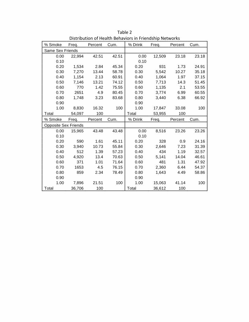
Table 2

Distribution of Health Behaviors in Friendship Networks

% Smoke Freq. Percent Cum. % Drink Freq. Percent Cum.

Same Sex Friends 0.00 22,994 42.51 42.51 0.00 12,509 23.18 23.18 0.10 0.10 0.20 1,534 2.84 45.34 0.20 931 1.73 24.91 0.30 7,270 13.44 58.78 0.30 5,542 10.27 35.18 0.40 1,154 2.13 60.91 0.40 1,064 1.97 37.15 0.50 7,146 13.21 74.12 0.50 7,713 14.3 51.45 0.60 770 1.42 75.55 0.60 1,135 2.1 53.55 0.70 2651 4.9 80.45 0.70 3,774 6.99 60.55 0.80 1,748 3.23 83.68 0.80 3,440 6.38 66.92 0.90 0.90 1.00 8,830 16.32 100 1.00 17,847 33.08 100

Total 54,097 100 Total 53,955 100

% Smoke Freq. Percent Cum. % Drink Freq. Percent Cum.

Opposite Sex Friends 0.00 15,965 43.48 43.48 0.00 8,516 23.26 23.26 0.10 0.10 0.20 590 1.61 45.11 0.20 328 0.9 24.16 0.30 3,940 10.73 55.84 0.30 2,646 7.23 31.39 0.40 512 1.39 57.23 0.40 434 1.19 32.57 0.50 4,920 13.4 70.63 0.50 5,141 14.04 46.61 0.60 371 1.01 71.64 0.60 481 1.31 47.92 0.70 1653 4.5 76.15 0.70 2,360 6.44 54.37 0.80 859 2.34 78.49 0.80 1,643 4.49 58.86 0.90 0.90 1.00 7,896 21.51 100 1.00 15,063 41.14 100

Total 36,706 100 Total 36,612 100

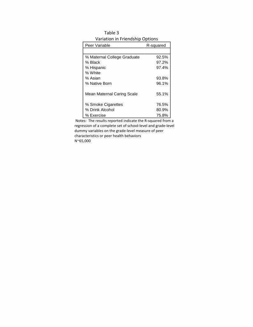
Table 3

Variation in Friendship Options

Peer Variable R-squared

% Maternal College Graduate 92.5% % Black 97.2% % Hispanic 97.4% % White % Asian 93.8% % Native Born 96.1% Mean Maternal Caring Scale 55.1% % Smoke Cigarettes 76.5% % Drink Alcohol 80.9% % Exercise 75.8%

Notes: The results reported indicate the R-squared from a

regression of a complete set of school-level and grade-level

dummy variables on the grade-level measure of peer

characteristics or peer health behaviors

N~65,000

Table 4

Balancing Tests of Friendship Sorting

Outcome Hispanic Hispanic Hispanic Hispanic Hispanic Hispanic

Specification OLS OLS OLS OLS OLS OLS

Fixed Effects None School School-Cluster

School-GradePair-

Cluster

School-GradePair-

Cluster-X

School-GradePair-

One Per Cluster-X

Friends' Maternal Education -0.032*** -0.022*** -0.003 -0.003

(0.006) (0.005) (0.002) (0.003)

Observations 65456 65456 65456 65456

R-squared 0.027 0.306 0.696 0.725

Outcome White White White White White White

Specification OLS OLS OLS OLS OLS OLS

Fixed Effects None School School-Cluster

School-GradePair-

Cluster

School-GradePair-

Cluster-X

School-GradePair-

One Per Cluster-X

Friends' Maternal Education 0.026*** 0.019*** 0.002 0.002

(0.007) (0.004) (0.002) (0.003)

Observations 65495 65456 65456 65456

R-squared 0.003 0.009 0.570 0.752

Outcome

Maternal

Education

Maternal

Education

Maternal

Education Maternal Education

Maternal

Education Maternal Education

Specification OLS OLS OLS OLS OLS OLS

Fixed Effects None School School-Cluster

School-GradePair-

Cluster

School-GradePair-

Cluster-X

School-GradePair-

One Per Cluster-X

Friends' Maternal Education 0.331*** 0.197*** 0.024 0.007 -0.010 0.018

(0.026) (0.021) (0.020) (0.014) (0.017) (0.072)

Observations 65456 65456 65456 65456 65456 49511

R-squared 0.061 0.123 0.530 0.586 0.869 0.975

Each set of rows and each column displays coefficients from separate regressions. All regressions control for grade-level fixed effects.

Table 4B

Balancing Tests of Friendship Sorting (Health Behaviors)

Outcome

Maternal

Education

Maternal

Education

Maternal

Education

Maternal

Education

Maternal

Education

Maternal

Education

Specification OLS OLS OLS OLS OLS OLS

Fixed Effects None School School-Cluster

School-GradePair-

Cluster

School-GradePair-

Cluster-X

School-GradePair-

One Per Cluster-X

Friends' Drinking -0.239*** -0.280*** -0.179*** -0.064 -0.059 -0.004

(0.057) (0.033) (0.046) (0.048) (0.066) (0.203)

Observations 53895 53895 53895 53895 54027 43797

R-squared 0.002 0.112 0.603 0.665 0.915 0.980

Outcome

Maternal

Education

Maternal

Education

Maternal

Education

Maternal

Education

Maternal

Education

Maternal

Education

Specification OLS OLS OLS OLS OLS OLS

Fixed Effects None School School-Cluster School-GradePair-

Cluster School-GradePair-

Cluster-X School-GradePair- One Per Cluster-X

Friends' Smoking -0.303*** -0.337*** -0.234*** -0.091* -0.031 -0.050

(0.074) (0.048) (0.059) (0.046) (0.072) (0.217)

Observations 54027 54027 54027 54027 53564 43895

R-squared 0.003 0.113 0.602 0.665 0.939 0.981

Outcome

Maternal

Education

Maternal

Education

Maternal

Education

Maternal

Education

Maternal

Education

Maternal

Education

Specification OLS OLS OLS OLS OLS OLS

Fixed Effects None School School-Cluster

School-GradePair-

Cluster

School-GradePair-

Cluster-X

School-GradePair-

One Per Cluster-X

Friends' Maternal Caring 0.216*** 0.157*** 0.082** 0.079** 0.039 0.053

(0.034) (0.023) (0.041) (0.035) (0.047) (0.137)

Observations 51017 51017 50289 51017 50289 41009

R-squared 0.002 0.112 0.601 0.602 0.938 0.980

Each set of rows and each column displays coefficients from separate regressions. All regressions control for grade-level fixed effects.

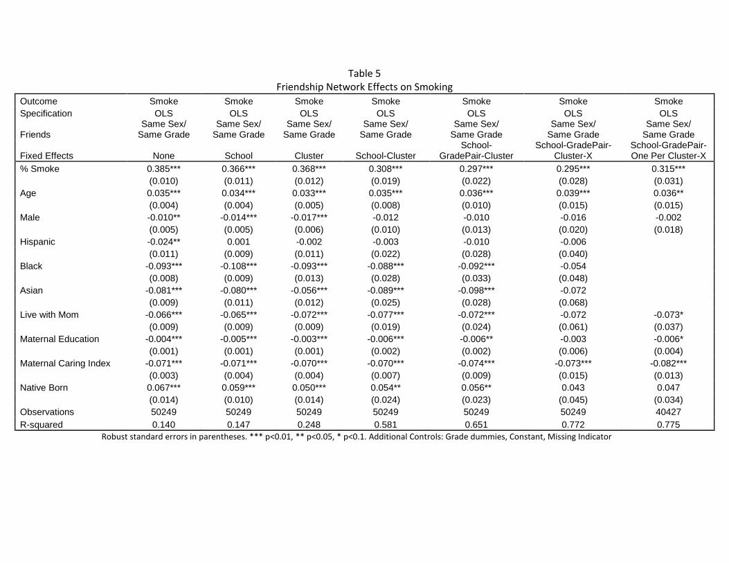
Table 5

Friendship Network Effects on Smoking

Outcome Smoke Smoke Smoke Smoke Smoke Smoke Smoke Specification OLS OLS OLS OLS OLS OLS OLS

Friends Same Sex/

Same Grade Same Sex/

Same Grade Same Sex/

Same Grade Same Sex/

Same Grade Same Sex/

Same Grade Same Sex/

Same Grade Same Sex/

Same Grade

Fixed Effects None School Cluster School-Cluster School-

GradePair-Cluster School-GradePair-

Cluster-X School-GradePair- One Per Cluster-X

% Smoke 0.385*** 0.366*** 0.368*** 0.308*** 0.297*** 0.295*** 0.315*** (0.010) (0.011) (0.012) (0.019) (0.022) (0.028) (0.031) Age 0.035*** 0.034*** 0.033*** 0.035*** 0.036*** 0.039*** 0.036** (0.004) (0.004) (0.005) (0.008) (0.010) (0.015) (0.015) Male -0.010** -0.014*** -0.017*** -0.012 -0.010 -0.016 -0.002 (0.005) (0.005) (0.006) (0.010) (0.013) (0.020) (0.018) Hispanic -0.024** 0.001 -0.002 -0.003 -0.010 -0.006 (0.011) (0.009) (0.011) (0.022) (0.028) (0.040) Black -0.093*** -0.108*** -0.093*** -0.088*** -0.092*** -0.054 (0.008) (0.009) (0.013) (0.028) (0.033) (0.048) Asian -0.081*** -0.080*** -0.056*** -0.089*** -0.098*** -0.072 (0.009) (0.011) (0.012) (0.025) (0.028) (0.068) Live with Mom -0.066*** -0.065*** -0.072*** -0.077*** -0.072*** -0.072 -0.073* (0.009) (0.009) (0.009) (0.019) (0.024) (0.061) (0.037) Maternal Education -0.004*** -0.005*** -0.003*** -0.006*** -0.006** -0.003 -0.006* (0.001) (0.001) (0.001) (0.002) (0.002) (0.006) (0.004) Maternal Caring Index -0.071*** -0.071*** -0.070*** -0.070*** -0.074*** -0.073*** -0.082*** (0.003) (0.004) (0.004) (0.007) (0.009) (0.015) (0.013) Native Born 0.067*** 0.059*** 0.050*** 0.054** 0.056** 0.043 0.047 (0.014) (0.010) (0.014) (0.024) (0.023) (0.045) (0.034) Observations 50249 50249 50249 50249 50249 50249 40427 R-squared 0.140 0.147 0.248 0.581 0.651 0.772 0.775

Robust standard errors in parentheses. *** p<0.01, ** p<0.05, * p<0.1. Additional Controls: Grade dummies, Constant, Missing Indicator

Table 6

Friendship Network Effects on Drinking

Outcome Drink Drink Drink Drink Drink Drink Drink Specification OLS OLS OLS OLS OLS OLS OLS

Friends Same Sex/

Same Grade Same Sex/

Same Grade Same Sex/

Same Grade Same Sex/

Same Grade Same Sex/

Same Grade Same Sex/

Same Grade Same Sex/

Same Grade

Fixed Effects None School Cluster School-Cluster School-GradePair-

Cluster School-GradePair-

Cluster-X School-GradePair- One Per Cluster-X

% Drink 0.329*** 0.302*** 0.316*** 0.253*** 0.239*** 0.235*** 0.284*** (0.011) (0.011) (0.013) (0.019) (0.022) (0.033) (0.089) Age 0.032*** 0.031*** 0.034*** 0.032*** 0.033*** 0.033** 0.025 (0.004) (0.004) (0.005) (0.009) (0.011) (0.015) (0.057) Male 0.005 0.002 0.003 0.007 0.006 0.009 0.022 (0.004) (0.004) (0.005) (0.010) (0.012) (0.020) (0.066) Hispanic 0.018* 0.026*** 0.033*** 0.044* 0.044 (0.010) (0.008) (0.011) (0.023) (0.027) Black -0.039*** -0.051*** -0.070*** -0.074*** -0.072** (0.010) (0.011) (0.015) (0.028) (0.028) Asian -0.101*** -0.118*** -0.078*** -0.081*** -0.078** (0.011) (0.012) (0.014) (0.026) (0.032) Live with Mom -0.066*** -0.065*** -0.071*** -0.069*** -0.075*** -0.050 -0.091 (0.009) (0.009) (0.009) (0.018) (0.021) (0.076) (0.250) Maternal Education -0.004*** -0.006*** -0.004** -0.006*** -0.006** 0.005 0.006 (0.001) (0.001) (0.001) (0.002) (0.002) (0.010) (0.022) Maternal Caring Index -0.064*** -0.064*** -0.064*** -0.063*** -0.062*** -0.065*** -0.069 (0.004) (0.003) (0.004) (0.007) (0.009) (0.014) (0.057) Native Born 0.086*** 0.084*** 0.070*** 0.079*** 0.083*** 0.077 0.118 (0.014) (0.013) (0.012) (0.022) (0.028) (0.052) (0.209) Observations 49656 49656 49656 49656 49656 49656 40570 R-squared 0.153 0.163 0.270 0.609 0.674 0.807 0.942

Robust standard errors in parentheses. *** p<0.01, ** p<0.05, * p<0.1. Additional Controls: Grade dummies, Constant, Missing Indicator

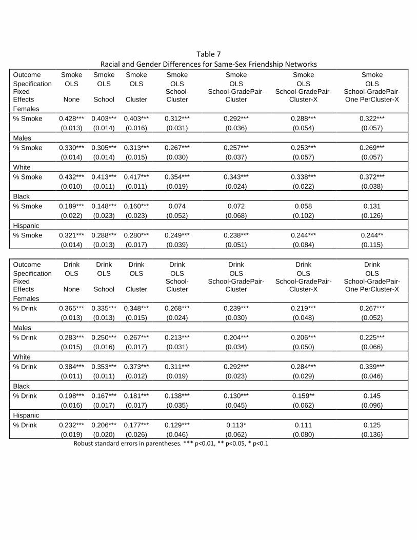
Table 7

Racial and Gender Differences for Same-Sex Friendship Networks

Outcome Smoke Smoke Smoke Smoke Smoke Smoke Smoke Specification OLS OLS OLS OLS OLS OLS OLS Fixed Effects None School Cluster

School-Cluster

School-GradePair-Cluster

School-GradePair- Cluster-X

School-GradePair- One PerCluster-X

Females % Smoke 0.428*** 0.403*** 0.403*** 0.312*** 0.292*** 0.288*** 0.322*** (0.013) (0.014) (0.016) (0.031) (0.036) (0.054) (0.057)

Males % Smoke 0.330*** 0.305*** 0.313*** 0.267*** 0.257*** 0.253*** 0.269*** (0.014) (0.014) (0.015) (0.030) (0.037) (0.057) (0.057)

White % Smoke 0.432*** 0.413*** 0.417*** 0.354*** 0.343*** 0.338*** 0.372*** (0.010) (0.011) (0.011) (0.019) (0.024) (0.022) (0.038)

Black % Smoke 0.189*** 0.148*** 0.160*** 0.074 0.072 0.058 0.131 (0.022) (0.023) (0.023) (0.052) (0.068) (0.102) (0.126)

Hispanic % Smoke 0.321*** 0.288*** 0.280*** 0.249*** 0.238*** 0.244*** 0.244** (0.014) (0.013) (0.017) (0.039) (0.051) (0.084) (0.115)

Outcome Drink Drink Drink Drink Drink Drink Drink Specification OLS OLS OLS OLS OLS OLS OLS Fixed Effects None School Cluster

School-Cluster

School-GradePair-Cluster

School-GradePair-Cluster-X

School-GradePair-One PerCluster-X

Females % Drink 0.365*** 0.335*** 0.348*** 0.268*** 0.239*** 0.219*** 0.267*** (0.013) (0.013) (0.015) (0.024) (0.030) (0.048) (0.052)

Males % Drink 0.283*** 0.250*** 0.267*** 0.213*** 0.204*** 0.206*** 0.225*** (0.015) (0.016) (0.017) (0.031) (0.034) (0.050) (0.066)

White % Drink 0.384*** 0.353*** 0.373*** 0.311*** 0.292*** 0.284*** 0.339*** (0.011) (0.011) (0.012) (0.019) (0.023) (0.029) (0.046)

Black % Drink 0.198*** 0.167*** 0.181*** 0.138*** 0.130*** 0.159** 0.145 (0.016) (0.017) (0.017) (0.035) (0.045) (0.062) (0.096)

Hispanic % Drink 0.232*** 0.206*** 0.177*** 0.129*** 0.113* 0.111 0.125 (0.019) (0.020) (0.026) (0.046) (0.062) (0.080) (0.136)

Robust standard errors in parentheses. *** p<0.01, ** p<0.05, * p<0.1

Table 8

Friendship Networks Effects of Smoking: Opposite Sex Friends

Outcome Smoke Smoke Smoke Smoke Smoke Smoke Specification OLS OLS OLS OLS OLS OLS

Friends Opp Sex/

Same Grade Opp Sex/

Same Grade Opp Sex/

Same Grade Opp Sex/

Same Grade Opp Sex/

Same Grade Opp Sex/

Same Grade

Fixed Effects None School Cluster School-

GradePair-Cluster School-GradePair-

Cluster-X School-GradePair- One Per Cluster-X

% Smoke 0.228*** 0.203*** 0.228*** 0.202*** 0.214*** 0.233 (0.010) (0.010) (0.011) (0.022) (0.037) (0.168) Age 0.040*** 0.037*** 0.038*** 0.029** 0.028 0.029 (0.005) (0.005) (0.006) (0.014) (0.021) (0.102) Male -0.014 -0.014 -0.023** -0.009 -0.023 -0.043 (0.010) (0.009) (0.011) (0.020) (0.033) (0.121) Hispanic -0.039** -0.004 -0.021 -0.021 (0.016) (0.013) (0.014) (0.030) Black -0.109*** -0.127*** -0.095*** -0.120*** (0.010) (0.011) (0.014) (0.034) Asian -0.089*** -0.092*** -0.048*** -0.070 (0.014) (0.016) -0.017 (0.046) Live with Mom -0.053*** -0.053*** -0.063*** -0.037 -0.054 -0.075 (0.012) (0.012) (0.014) (0.032) (0.099) (0.499) Maternal Education -0.006*** -0.007*** -0.005*** -0.009*** -0.004 -0.001 (0.001) (0.001) (0.001) (0.003) (0.009) (0.053) Maternal Caring Index -0.077*** -0.078*** -0.075*** -0.073*** -0.075*** -0.065 (0.004) (0.004) (0.005) (0.010) (0.017) (0.109) Native Born 0.077*** 0.066*** 0.062*** 0.054 0.047 0.048 (0.019) (0.015) (0.020) (0.035) (0.066) (0.319) Observations 33807 33807 33807 33807 33807 26346 R-squared 0.083 0.096 0.225 0.663 0.796 0.957

Robust standard errors in parentheses. *** p<0.01, ** p<0.05, * p<0.1

Table 9

Friendship Networks Effects of Drinking: Opposite Sex Friends

Outcome Drink Drink Drink Drink Drink Drink Drink Specification OLS OLS OLS OLS OLS OLS OLS

Friends Opp Sex/

Same Grade Opp Sex/

Same Grade Opp Sex/

Same Grade Opp Sex/

Same Grade Opp Sex/

Same Grade Opp Sex/

Same Grade Opp Sex/

Same Grade

Fixed Effects None School Cluster School-Cluster School-

GradePair-Cluster School-GradePair-

Cluster-X School-GradePair-

Cluster-X % Drink 0.211*** 0.180*** 0.213*** 0.183*** 0.170*** 0.168*** 0.156 (0.011) (0.010) (0.013) (0.020) (0.024) (0.040) (0.183) Age 0.039*** 0.035*** 0.038*** 0.032*** 0.030** 0.025 -0.000 (0.006) (0.006) (0.006) (0.012) (0.013) (0.022) (0.104) Male 0.017** 0.017** 0.012 0.011 0.011 0.010 0.016 (0.007) (0.007) (0.008) (0.013) (0.016) (0.026) (0.125) Hispanic 0.017 0.020** 0.021 0.038 0.034 (0.013) (0.010) (0.014) (0.025) (0.034) Black -0.049*** -0.070*** -0.061*** -0.056** -0.067* (0.012) (0.012) (0.014) (0.028) (0.034) Asian -0.113*** -0.139*** -0.072*** -0.072** -0.079* (0.014) (0.014) (0.015) (0.035) (0.043) Live with Mom -0.069*** -0.070*** -0.085*** -0.091*** -0.090*** -0.154* -0.117 (0.011) (0.010) (0.012) (0.024) (0.030) (0.089) (0.478) Maternal Education -0.006*** -0.009*** -0.006*** -0.008*** -0.008*** 0.000 -0.003 (0.002) (0.001) (0.002) (0.003) (0.003) (0.010) (0.065) Maternal Caring Index -0.063*** -0.063*** -0.062*** -0.060*** -0.058*** -0.059*** -0.066 (0.004) (0.004) (0.005) (0.009) (0.011) (0.019) (0.109) Native Born 0.113*** 0.112*** 0.111*** 0.129*** 0.140*** 0.143** 0.161 (0.020) (0.018) (0.021) (0.031) (0.038) (0.066) (0.337) Observations 33702 33702 33702 33702 33702 33702 26259 R-squared 0.114 0.132 0.264 0.627 0.691 0.816 0.961

Robust standard errors in parentheses. *** p<0.01, ** p<0.05, * p<0.1

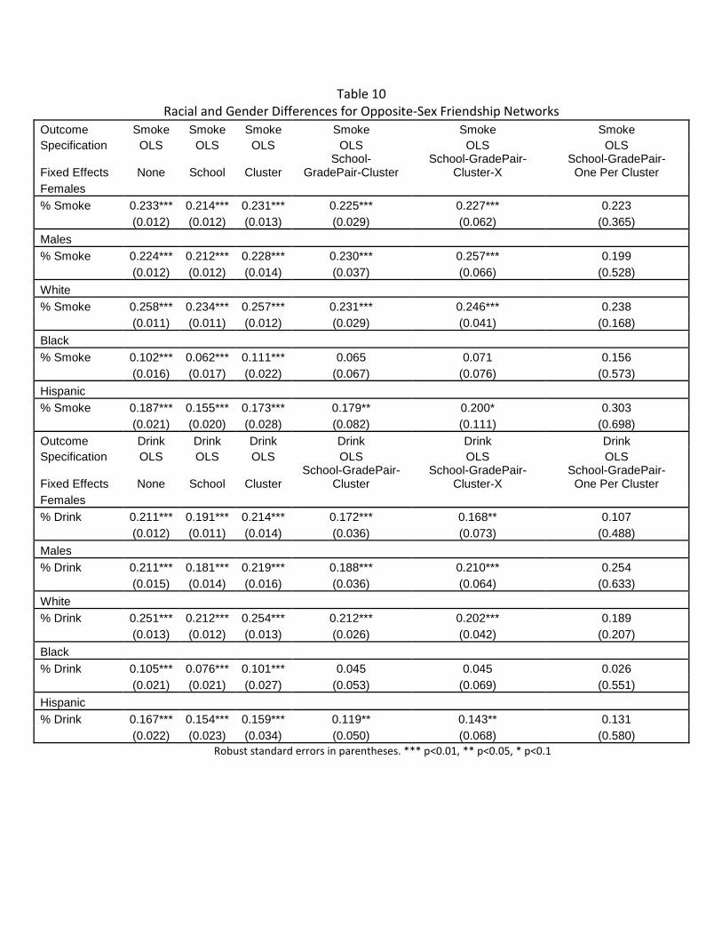
Table 10

Racial and Gender Differences for Opposite-Sex Friendship Networks

Outcome Smoke Smoke Smoke Smoke Smoke Smoke Specification OLS OLS OLS OLS OLS OLS

Fixed Effects None School Cluster School-

GradePair-Cluster School-GradePair-

Cluster-X School-GradePair- One Per Cluster

Females % Smoke 0.233*** 0.214*** 0.231*** 0.225*** 0.227*** 0.223 (0.012) (0.012) (0.013) (0.029) (0.062) (0.365)

Males % Smoke 0.224*** 0.212*** 0.228*** 0.230*** 0.257*** 0.199 (0.012) (0.012) (0.014) (0.037) (0.066) (0.528)

White % Smoke 0.258*** 0.234*** 0.257*** 0.231*** 0.246*** 0.238 (0.011) (0.011) (0.012) (0.029) (0.041) (0.168)

Black % Smoke 0.102*** 0.062*** 0.111*** 0.065 0.071 0.156 (0.016) (0.017) (0.022) (0.067) (0.076) (0.573)

Hispanic % Smoke 0.187*** 0.155*** 0.173*** 0.179** 0.200* 0.303 (0.021) (0.020) (0.028) (0.082) (0.111) (0.698) Outcome Drink Drink Drink Drink Drink Drink Specification OLS OLS OLS OLS OLS OLS

Fixed Effects None School Cluster School-GradePair-

Cluster School-GradePair-

Cluster-X School-GradePair- One Per Cluster

Females % Drink 0.211*** 0.191*** 0.214*** 0.172*** 0.168** 0.107 (0.012) (0.011) (0.014) (0.036) (0.073) (0.488)

Males % Drink 0.211*** 0.181*** 0.219*** 0.188*** 0.210*** 0.254 (0.015) (0.014) (0.016) (0.036) (0.064) (0.633)

White % Drink 0.251*** 0.212*** 0.254*** 0.212*** 0.202*** 0.189 (0.013) (0.012) (0.013) (0.026) (0.042) (0.207)

Black % Drink 0.105*** 0.076*** 0.101*** 0.045 0.045 0.026 (0.021) (0.021) (0.027) (0.053) (0.069) (0.551)

Hispanic % Drink 0.167*** 0.154*** 0.159*** 0.119** 0.143** 0.131 (0.022) (0.023) (0.034) (0.050) (0.068) (0.580)

Robust standard errors in parentheses. *** p<0.01, ** p<0.05, * p<0.1

Appendix Tables

Table 1A

Predictors of Dropped Sample

Outcome Means No ID No Friend

Nominations No Found

Nominations Any Drop

No Same Grade

No Same Grade/ Gender Friends

Means 0.047 0.14 0.2 0.24 0.065 0.129 Fixed Effects School School School School School School Age 15 0.005*** 0.026*** 0.016*** 0.040*** 0.032*** 0.024*** (0.001) (0.003) (0.002) (0.003) (0.002) (0.002) Male 0.502 0.007*** 0.072*** 0.016*** 0.083*** 0.030*** 0.007*** (0.001) (0.005) (0.002) (0.006) (0.003) (0.002) Hispanic 0.155 0.004 0.014** 0.002 0.020*** -0.006 -0.001 (0.003) (0.006) (0.004) (0.007) (0.006) (0.004) Black 0.19 0.007*** 0.037*** 0.027*** 0.060*** 0.017*** 0.013*** (0.002) (0.006) (0.005) (0.007) (0.005) (0.004) Asian 0.056 -0.003 0.002 0.001 0.004 -0.038*** -0.017*** (0.004) (0.009) (0.009) (0.013) (0.008) (0.005)

Native Born 0.9 -0.003 -0.023*** -0.027*** -

0.042*** -0.007 -0.018*** (0.003) (0.005) (0.006) (0.007) (0.008) (0.006) Live with Mom 0.92 0.037*** 0.292*** 0.059*** 0.306*** 0.152*** 0.067*** (0.011) (0.019) (0.017) (0.023) (0.008) (0.006)

Mom Education 13.36 -0.000 -0.001* -0.001 -

0.002*** -0.001** -0.001*** (0.000) (0.001) (0.000) (0.001) (0.000) (0.000)

Mom Care 4.76 -0.002* -0.009*** -0.005*** -

0.013*** -0.006*** -0.006*** (0.001) (0.002) (0.002) (0.002) (0.002) (0.002) Smoke 0.36 0.005** 0.007** 0.011*** 0.017*** 0.024*** 0.013*** (0.002) (0.003) (0.002) (0.003) (0.003) (0.002)

Drink 0.55 0.000 -0.020*** -0.001 -

0.017*** 0.001 -0.004 (0.001) (0.003) (0.002) (0.003) (0.003) (0.002) % Black 0.19 -0.010 -0.110 0.015 -0.097 -0.046 -0.043 (0.031) (0.084) (0.051) (0.107) (0.036) (0.035) % Hispanic 0.16 0.036 0.089 0.067 0.162* -0.065 -0.039 (0.070) (0.084) (0.054) (0.097) (0.049) (0.049) % Mom Grad 0.32 0.040 -0.064 -0.032 -0.062 0.002 -0.035 (0.035) (0.052) (0.032) (0.065) (0.042) (0.036) % Smoke 0.36 0.060 0.042 0.011 0.072 -0.092** -0.061* (0.042) (0.055) (0.037) (0.074) (0.039) (0.032) % Drink 0.55 -0.000 -0.089 0.012 -0.047 0.103*** 0.058 (0.027) (0.056) (0.039) (0.066) (0.039) (0.038)

Constant -0.081** -0.458*** -0.161*** -

0.542*** -0.576*** -0.317*** (0.032) (0.049) (0.040) (0.060) (0.039) (0.039) Observations 88995 84789 73363 88995 59470 59470 R-squared 0.173 0.188 0.210 0.245 0.246 0.122

Notes: Grade fixed effects controls and missing indicators are now shown. “No ID” is a binary variable indicating

whether the respondent received an identification number in the survey. “No Friend Nominations” is a binary

variable indicating whether the respondent made zero friend nominations. “No Found Nominations” is a binary

variable indicating whether the respondent nominated friends who were not able to be matched within sample

(such as friends outside of school).

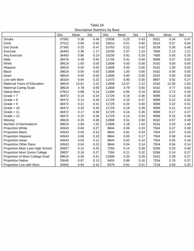
Table 2A

Descriptive Statistics by Race

Obs Mean Std. Obs Mean Std. Obs Mean Std. Smoke 37592 0.39 0.49 10938 0.25 0.43 8331 0.34 0.47 Drink 37512 0.56 0.50 10910 0.51 0.50 8314 0.57 0.50 Get Drunk 37365 0.33 0.47 10793 0.22 0.42 8239 0.30 0.46 Exercise 36493 2.38 1.17 10239 2.07 1.24 7606 2.13 1.21 Any Exercise 36493 0.96 0.19 10239 0.91 0.29 7606 0.93 0.26 Male 38476 0.48 0.50 11745 0.41 0.49 9096 0.47 0.50 White 38619 1.00 0.00 11808 0.00 0.00 9162 0.00 0.00 Hispanic 38619 0.00 0.00 11808 0.00 0.00 9162 1.00 0.00 Black 38619 0.00 0.00 11808 1.00 0.00 9162 0.00 0.00 Asian 38619 0.00 0.00 11808 0.00 0.00 9162 0.00 0.00 Live with Mom 38334 0.94 0.23 11470 0.90 0.30 8897 0.92 0.27 Maternal Years of Education 38619 13.61 2.22 11808 13.47 2.12 9162 12.30 2.63 Maternal Caring Scale 38619 4.78 0.59 11808 4.79 0.60 9162 4.77 0.63 Native Born 37813 0.98 0.14 11496 0.96 0.19 8836 0.72 0.45 Grade = 7 38472 0.14 0.34 11729 0.16 0.36 9089 0.13 0.34 Grade = 8 38472 0.14 0.34 11729 0.16 0.37 9089 0.12 0.32 Grade = 9 38472 0.21 0.41 11729 0.20 0.40 9089 0.22 0.41 Grade = 10 38472 0.20 0.40 11729 0.18 0.39 9089 0.21 0.41 Grade = 11 38472 0.17 0.38 11729 0.16 0.36 9089 0.17 0.37 Grade = 12 38472 0.15 0.36 11729 0.14 0.34 9089 0.15 0.36 Missing 38619 0.35 0.48 11808 0.51 0.50 9162 0.57 0.49 Number of Nominations 38619 2.58 1.52 11808 2.18 1.52 9162 2.03 1.49 Proportion White 34543 0.84 0.27 9844 0.09 0.24 7504 0.27 0.39 Proportion Black 34543 0.03 0.13 9844 0.81 0.33 7504 0.07 0.20 Proportion Hispanic 34543 0.06 0.18 9844 0.05 0.17 7504 0.58 0.44 Proportion Asian 34543 0.03 0.12 9844 0.02 0.10 7504 0.05 0.18 Proportion Other Race 34543 0.04 0.13 9844 0.04 0.14 7504 0.04 0.14 Proportion Mom Less High School 28837 0.12 0.25 7260 0.14 0.28 5266 0.33 0.40 Proportion Mom Some College 28837 0.18 0.27 7260 0.21 0.32 5266 0.14 0.27 Proportion of Mom College Grad 38619 0.36 0.31 11808 0.33 0.29 9162 0.28 0.27 Proportion Native 33645 0.97 0.13 9455 0.96 0.16 7204 0.76 0.37 Proportion Live with Mom 33945 0.94 0.16 9379 0.91 0.21 7218 0.93 0.20

Table 3A

Predictors of “Unusual Type”—Single Cluster Membership

Outcome Single Cluster

Single Cluster

Single Cluster

Single Cluster

Single Cluster

Cluster Friend Xs X, School X,S, Own Xs X,S Cohort X,S,X, Cohort Mean of dependent variable 0.06 0.32 0.37 0.44 0.53 Fixed Effects School School School School School Age -0.007*** -0.033*** -0.035*** -0.036*** -0.042*** (0.002) (0.004) (0.004) (0.004) (0.004) Male 0.006** -0.005 -0.014** -0.015*** -0.017*** (0.003) (0.006) (0.006) (0.006) (0.006) Hispanic 0.020*** 0.014 0.013 0.044*** 0.078*** (0.005) (0.011) (0.012) (0.016) (0.021) Black 0.015** 0.029 0.030 0.041 0.043 (0.007) (0.021) (0.023) (0.025) (0.026) Asian 0.079*** 0.091*** 0.097*** 0.132*** 0.192*** (0.012) (0.018) (0.018) (0.025) (0.027) Native Born -0.013** 0.000 0.006 0.005 0.006 (0.006) (0.010) (0.009) (0.010) (0.011) Live with Mom -0.007* -0.049*** -0.069*** -0.153*** -0.162*** (0.004) (0.008) (0.009) (0.011) (0.012) Mom Educatoin -0.000 -0.000 -0.000 0.012*** 0.013*** (0.000) (0.001) (0.001) (0.002) (0.002) Mom Care 0.000 0.000 0.002 0.003 0.003 (0.001) (0.003) (0.003) (0.003) (0.003) Smoke -0.009*** -0.030*** -0.033*** -0.030*** -0.031*** (0.002) (0.005) (0.005) (0.005) (0.005) Drink -0.003 -0.006 -0.007 -0.004 -0.001 (0.003) (0.005) (0.004) (0.005) (0.005) % Black 0.012 -0.023 -0.094 -0.090 -0.151* (0.028) (0.055) (0.072) (0.064) (0.085) % Hispanic 0.035 0.097 0.049 0.077 -0.051 (0.050) (0.087) (0.094) (0.087) (0.097) % Mom College Grad 0.042 -0.081 -0.099 -0.038 -0.085 (0.038) (0.069) (0.084) (0.070) (0.078) % Smoke 0.024 0.037 -0.001 0.064 0.040 (0.028) (0.058) (0.067) (0.074) (0.076) % Drink -0.058** -0.125*** -0.109** -0.144*** -0.099* (0.028) (0.044) (0.053) (0.054) (0.057) Constant 0.207*** 0.972*** 1.084*** 1.040*** 1.242*** (0.042) (0.063) (0.070) (0.070) (0.071) Observations 59470 59470 59470 59470 59470 R-squared 0.068 0.087 0.078 0.096 0.092

Robust standard errors in parentheses. *** p<0.01, ** p<0.05, * p<0.1. Grade fixed effects not shown.

Table 5A

Analysis of the Change in Composition of the Sample Due to Singleton Clusters

Outcome Smoke Smoke Smoke Smoke Smoke Smoke Smoke Group None School Cluster School/Cluster School-Cluster School-Cluster-GradePair School-Cluster-GradePair-Xs % Smoke 0.385*** 0.366*** 0.368*** 0.348*** 0.308*** 0.297*** 0.295*** (0.010) (0.011) (0.012) (0.012) (0.019) (0.022) (0.028) Observations 50959 50959 50959 50959 50959 50959 50959 R-squared 0.135 0.143 0.245 0.252 0.580 0.649 0.761 Outcome Smoke Smoke Smoke Smoke Smoke Smoke Smoke Group None School Cluster School/Cluster School-Cluster School-Cluster-GradePair School-Cluster-GradePair-Xs % Smoke 0.385*** 0.366*** 0.383*** 0.363*** 0.364*** 0.358*** 0.357*** (0.010) (0.012) (0.011) (0.011) (0.011) (0.012) (0.011) Observations 50249 50249 46842 46842 32032 28557 20120 R-squared 0.140 0.147 0.140 0.148 0.140 0.139 0.142 Outcome Smoke Smoke Smoke Smoke Smoke Smoke Smoke Group None School Cluster School/Cluster School-Cluster School-Cluster-GradePair School-Cluster-GradePair-Xs % Smoke 0.385*** 0.357*** 0.357*** 0.323*** 0.299*** 0.291*** 0.295*** (0.010) (0.011) (0.011) (0.012) (0.016) (0.018) (0.018) Observations 50249 20120 20120 20120 20120 20120 20120

R-squared 0.140 0.142 0.142 0.190 0.352 0.403 0.449

Outcome Drink Drink Drink Drink Drink Drink Drink Group None School Cluster School/Cluster School-Cluster School-Cluster-GradePair School-Cluster-GradePair-Xs % Drink 0.329*** 0.302*** 0.315*** 0.286*** 0.253*** 0.240*** 0.235*** (0.011) (0.011) (0.013) (0.013) (0.019) (0.022) (0.029) Observations 50019 50019 50019 50019 50019 50019 50019 R-squared 0.153 0.163 0.270 0.280 0.608 0.673 0.790 Outcome Drink Drink Drink Drink Drink Drink Drink Group None School Cluster School/Cluster School-Cluster School-Cluster-GradePair School-Cluster-GradePair-Xs % Drink 0.329*** 0.302*** 0.324*** 0.297*** 0.308*** 0.304*** 0.296*** (0.011) (0.011) (0.012) (0.012) (0.013) (0.013) (0.013) Observations 50019 50019 46616 46616 31878 28421 20021 R-squared 0.153 0.163 0.153 0.164 0.146 0.147 0.143 Outcome Drink Drink Drink Drink Drink Drink Drink Group None School Cluster School/Cluster School-Cluster School-Cluster-GradePair School-Cluster-GradePair-Xs % Drink 0.329*** 0.296*** 0.296*** 0.257*** 0.233*** 0.225*** 0.235*** (0.011) (0.013) (0.013) (0.014) (0.018) (0.018) (0.019) Observations 50019 20021 20021 20021 20021 20021 20021

R-squared 0.153 0.143 0.143 0.199 0.365 0.413 0.467 Robust standard errors in parentheses. *** p<0.01, ** p<0.05, * p<0.1.

Each column and row is from a separate regression. The first row of each set repeats the results from

Table 5 (6). The second row reproduces the Column 1 results with the non-singleton samples. The third

row presents results of each specification with the final column’s sample