Eurographics Symposium on Rendering 2009Hendrik Lensch and Peter-Pike Sloan(Guest Editors)

Volume 28 (2009), Number 4

Estimating Specular Roughness and Anisotropy fromSecond Order Spherical Gradient Illumination

Abhijeet Ghosh Tongbo Chen Pieter Peers Cyrus A. Wilson Paul Debevec

University of Southern California,Institute for Creative Technologies

AbstractThis paper presents a novel method for estimating specular roughness and tangent vectors, per surface point, frompolarized second order spherical gradient illumination patterns. We demonstrate that for isotropic BRDFs, onlythree second order spherical gradients are sufficient to robustly estimate spatially varying specular roughness.For anisotropic BRDFs, an additional two measurements yield specular roughness and tangent vectors per surfacepoint. We verify our approach with different illumination configurations which project both discrete and continuousfields of gradient illumination. Our technique provides a direct estimate of the per-pixel specular roughness andthus does not require off-line numerical optimization that is typical for the measure-and-fit approach to classicalBRDF modeling.

Categories and Subject Descriptors (according to ACM CCS): Computer Graphics [I.3.7]: Three-DimensionalGraphics and Realism—

1. Introduction

Measuring the appearance of real materials is an active re-search area in computer graphics. Often the appearance isdescribed by the bidirectional reflectance distribution func-tion (BRDF) [NRH∗77], a 4D function that relates the ra-tio of reflectance between the incident and outgoing direc-tions for a single surface point. Usually these BRDF mod-els depend on a sparse set of non-linear parameters thatroughly correspond to albedo, specular roughness, surfacenormal, and tangent directions. Measuring and fitting theseparameters for a particular material model often requires adense sampling of incident and outgoing lighting directions.In many cases fitting the parameters of an a-priori chosenBRDF model to the observed measurements relies on com-plex fragile non-linear optimization procedures.

Recently a number of methods have been proposed thatestimate fundamental parameters of appearance, such as nor-mal direction and albedo, without assuming an a-priori mate-rial model. Instead they rely on general properties shared bymany physical materials such as symmetry [ZBK02, AK07,MHP∗07, AZK08, HLHZ08]. The work presented here ismost related to [MHP∗07], where it is shown that the firstorder spherical statistics of the reflectance under distant il-

lumination correspond to the normal and reflection vectorfor diffuse and specular materials respectively. Furthermore,Ma et al. [MHP∗07] demonstrate that the first order statis-tics can be efficiently measured using linear gradient illumi-nation conditions. In this work, we build upon Ma et al.’swork to estimate a per-pixel specular roughness using polar-ized second order spherical gradients that provide measure-ments of the variance about the mean (i.e., reflection vector).We demonstrate that for isotropic BRDFs, only three addi-tional axis-aligned second order spherical gradient illumina-tion patterns are sufficient for a robust estimate of per pixelspecular roughness (Figure 1). We also demonstrate that byusing the five second order spherical harmonics, related tothe second order spherical gradient illumination patterns, re-liable estimates of the specular roughness and tangent di-rections of general anisotropic BRDFs are possible. Using alookup table, these estimated high order statistics can thenbe directly translated to the parameters of any BRDF modelof choice.

An example of a direct application of our method is theestimation of spatially varying reflectance parameters of ar-bitrary objects. Furthermore, since the proposed method re-lies on only up to nine distinct illumination conditions with

c 2009 The Author(s)Journal compilation c 2009 The Eurographics Association and Blackwell Publishing Ltd.Published by Blackwell Publishing, 9600 Garsington Road, Oxford OX4 2DQ, UK and350 Main Street, Malden, MA 02148, USA.

Ghosh et al. / Estimating Specular Roughness and Anisotropy from Second Order Spherical Gradient Illumination

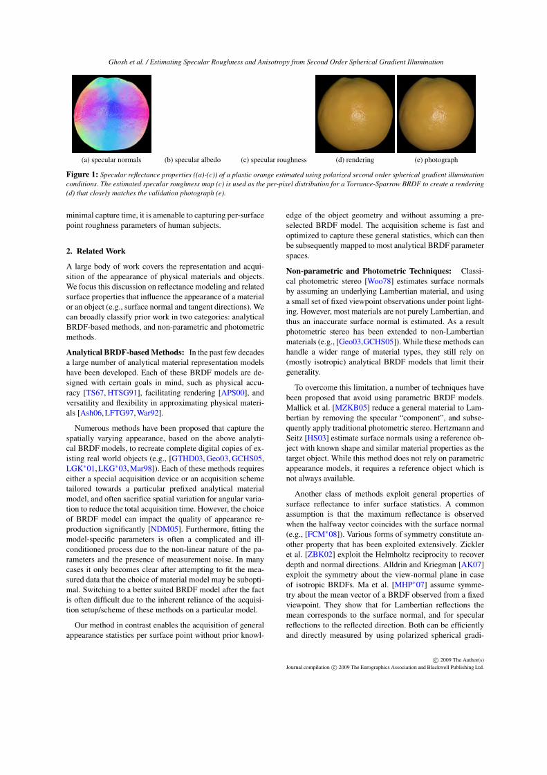
(a) specular normals (b) specular albedo (c) specular roughness (d) rendering (e) photograph

Figure 1: Specular reflectance properties ((a)-(c)) of a plastic orange estimated using polarized second order spherical gradient illuminationconditions. The estimated specular roughness map (c) is used as the per-pixel distribution for a Torrance-Sparrow BRDF to create a rendering(d) that closely matches the validation photograph (e).

minimal capture time, it is amenable to capturing per-surfacepoint roughness parameters of human subjects.

2. Related Work

A large body of work covers the representation and acqui-sition of the appearance of physical materials and objects.We focus this discussion on reflectance modeling and relatedsurface properties that influence the appearance of a materialor an object (e.g., surface normal and tangent directions). Wecan broadly classify prior work in two categories: analyticalBRDF-based methods, and non-parametric and photometricmethods.

Analytical BRDF-based Methods: In the past few decadesa large number of analytical material representation modelshave been developed. Each of these BRDF models are de-signed with certain goals in mind, such as physical accu-racy [TS67, HTSG91], facilitating rendering [APS00], andversatility and flexibility in approximating physical materi-als [Ash06, LFTG97, War92].

Numerous methods have been proposed that capture thespatially varying appearance, based on the above analyti-cal BRDF models, to recreate complete digital copies of ex-isting real world objects (e.g., [GTHD03, Geo03, GCHS05,LGK∗01,LKG∗03,Mar98]). Each of these methods requireseither a special acquisition device or an acquisition schemetailored towards a particular prefixed analytical materialmodel, and often sacrifice spatial variation for angular varia-tion to reduce the total acquisition time. However, the choiceof BRDF model can impact the quality of appearance re-production significantly [NDM05]. Furthermore, fitting themodel-specific parameters is often a complicated and ill-conditioned process due to the non-linear nature of the pa-rameters and the presence of measurement noise. In manycases it only becomes clear after attempting to fit the mea-sured data that the choice of material model may be subopti-mal. Switching to a better suited BRDF model after the factis often difficult due to the inherent reliance of the acquisi-tion setup/scheme of these methods on a particular model.

Our method in contrast enables the acquisition of generalappearance statistics per surface point without prior knowl-

edge of the object geometry and without assuming a pre-selected BRDF model. The acquisition scheme is fast andoptimized to capture these general statistics, which can thenbe subsequently mapped to most analytical BRDF parameterspaces.

Non-parametric and Photometric Techniques: Classi-cal photometric stereo [Woo78] estimates surface normalsby assuming an underlying Lambertian material, and usinga small set of fixed viewpoint observations under point light-ing. However, most materials are not purely Lambertian, andthus an inaccurate surface normal is estimated. As a resultphotometric stereo has been extended to non-Lambertianmaterials (e.g., [Geo03,GCHS05]). While these methods canhandle a wider range of material types, they still rely on(mostly isotropic) analytical BRDF models that limit theirgenerality.

To overcome this limitation, a number of techniques havebeen proposed that avoid using parametric BRDF models.Mallick et al. [MZKB05] reduce a general material to Lam-bertian by removing the specular “component”, and subse-quently apply traditional photometric stereo. Hertzmann andSeitz [HS03] estimate surface normals using a reference ob-ject with known shape and similar material properties as thetarget object. While this method does not rely on parametricappearance models, it requires a reference object which isnot always available.

Another class of methods exploit general properties ofsurface reflectance to infer surface statistics. A commonassumption is that the maximum reflectance is observedwhen the halfway vector coincides with the surface normal(e.g., [FCM∗08]). Various forms of symmetry constitute an-other property that has been exploited extensively. Zickleret al. [ZBK02] exploit the Helmholtz reciprocity to recoverdepth and normal directions. Alldrin and Kriegman [AK07]exploit the symmetry about the view-normal plane in caseof isotropic BRDFs. Ma et al. [MHP∗07] assume symme-try about the mean vector of a BRDF observed from a fixedviewpoint. They show that for Lambertian reflections themean corresponds to the surface normal, and for specularreflections to the reflected direction. Both can be efficientlyand directly measured by using polarized spherical gradi-

c 2009 The Author(s)Journal compilation c 2009 The Eurographics Association and Blackwell Publishing Ltd.

Ghosh et al. / Estimating Specular Roughness and Anisotropy from Second Order Spherical Gradient Illumination

ent illumination. Holroyd et al. [HLHZ08] assume a similartype of symmetry, but use a dense sampling to resolve boththe normal direction as well as tangent vectors per surfacepoint.

While these methods do not rely on a parametric model,they do not provide complete information regarding the sur-face reflectance. Lawrence et al. [LBAD∗06] used inverseshade trees and an optimization scheme coined ACLS to de-compose the spatially varying material properties of planarsamples from dense hemispherical samplings in a collec-tion of 1D curves and 2D textures. Alldrin et al. [AZK08]also employ ACLS to compute bivariate representations ofisotropic surface appearances, including surface normals. Fi-nally, Zickler et al. [ZREB06] share reflectance informa-tion from different surface points to create a dense non-parametric reconstruction of appearance.

All of the above methods either require a dense samplingof the lighting directions, integrate information over multiplesurface points, or deliver incomplete appearance informa-tion. The method proposed in this work extends [MHP∗07]to capture the second order statistics of surface reflection in-dependently per surface point. We show that these secondorder statistics correspond to specular roughness and the tan-gent vectors for specular reflections. These statistics can bereadily captured by extending the linear spherical gradientsof Ma et al. with second order spherical gradients. As such itrequires only a few observations, while delivering statisticssuitable for creating complete appearance descriptions.

3. Theoretical Background

In this section, we introduce the necessary notations anddefinitions that we need to infer specular roughness andanisotropy from second order gradient illumination. We firstrecap the definitions of moments on general 1D functions,which are then extended to a spherical domain. Armed withthese definitions, we then show how these moments canbe used to infer specular roughness. Finally, we show theconnection between spherical harmonics and spherical mo-ments, and how they can be used to measure and infer rough-ness and anisotropy.

0th, 1st, and 2nd Moments In statistics the zeroth, first andsecond moments of a general 1D function f(x) correspond tothe total energy α , mean µ , and variance σ2 of that function.These moments can be directly computed from the inner-products of the function f(x) and a constant function (g(x) =1), linear gradient (g(x) = x), and quadratic function (g(x) =x2), denoted by L0, L1, and L2 respectively:

α =

f(x)dx,

= L0, (1)

µ =

xf(x)α

dx,

=1α

x f(x)dx,

=L1L0

, (2)

σ2 =

(x−µ)2 f(x)α

dx,

=1α

x2 f(x)dx−2µ

x f(x)dx+ µ2

f(x)dx

,

=1α

L2−2µL1 + µ2L0

,

=L2L0−

L21

L20. (3)

0th, 1st, and 2nd Spherical Moments We can extend thesemoments to the spherical domain by redefining L0, L1, andL2 on the sphere Ω. This can be compactly denoted using thefollowing vector notation:

L0 =

Ωf(ω)dω, (4)

L1 =

Ωω f(ω)dω, (5)

L2 =

ΩωωT f(ω)dω, (6)

where ω = [ωx,ωy,ωz] ∈Ω, and each integration is with re-spect to solid angle. Thus: ω2

x +ω2y +ω2

z = 1. Note that ωωT

is the generalization of the quadratic function x2 to the spher-ical domain, and is a symmetric 3× 3 matrix. FurthermoreL0 is a scalar, L1 is a vector of length 3, and L2 is a 3× 3symmetric matrix. Applying these to Equations (1), (2), and(3), yield the 0th, 1st, and 2nd order spherical moments. Thethree linear spherical gradient of Ma et al. [MHP∗07] cor-respond to ω . Likewise, ωωT defines six new second orderspherical gradients. On the diagonal of this matrix are thequadratic gradients ω2

x , ω2y , and ω2

z . On the off-diagonal ele-ments are the mixed linear gradients: ωxωy, ωxωz, and ωyωz.

Specular Roughness Ma et al. [MHP∗07] demonstratedthat for specular reflections, the zeroth and first order mo-ments correspond to the specular albedo and reflection vec-tor. In this work, we argue that the second moment un-der specular reflections is directly proportional to specularroughness. Note that this “specular roughness” is indepen-dent of a chosen analytical BRDF model. While the exactrelation to a particular BRDF model’s specular parametersis highly model dependent, it is still instructive to verify thecorrelations of the 2nd moment and the specular parame-ters of an analytical model. For example, consider the WardBRDF [War92]:

R(h) = c · e

hxhzσx

2+

hy

hzσy

2

, (7)

where c is a normalization constant, h = (hx,hy,hz) is thehalfway vector between incident ωi and outgoing ωo di-

c 2009 The Author(s)Journal compilation c 2009 The Eurographics Association and Blackwell Publishing Ltd.

Ghosh et al. / Estimating Specular Roughness and Anisotropy from Second Order Spherical Gradient Illumination

rections, and σx and σy are the anisotropic specular rough-ness parameters. By definition, R is normalized, and con-sequently α = 1. For simplicity, lets assume that the localshading frame (reflected direction + tangent directions) areknown, and the spherical gradients are defined in this frame(this can be accomplished by an appropriate rotation suchthat the reflection direction is aligned with [0,0,1]). Then,µ = [0,0,1]. In this case Equation (3) simplifies to σ2 = L2,and:

L2 =

ΩωωT R(ω)dω ∼

σ2

x 0 00 σ2

y 00 0 σ2

z

. (8)

Intuitively, Equation (7) closely resembles a normal distri-bution for which the 2nd moment corresponds to the vari-ance (the diagonal elements). The off-diagonal element inL2 are zero because the gradients are axis aligned. Notethat σ2

z depends on the values of σ2x and σ2

y . The exactvalue of σ2

z does not have a direct physical meaning, hencewe will ignore this value. Practically, the above states thatthe observed radiance is proportional to the specular rough-ness, when illuminating a surface point with shading framealigned quadratic gradients ω2

x and ω2y .

2nd Order Spherical Harmonics The above discussionassumes that the gradients are aligned with the local shadingframe. However, this shading frame is most likely not knownbeforehand. Furthermore, every surface point has a poten-tially different shading frame orientation. Additionally, thesix second order spherical gradients do not form an orthog-onal spherical basis, and as such are not optimal in termsof number of patterns. Ideally, we would like to capture theresponses under some optimal (i.e., orthogonal) canonicalspherical basis illumination, from which the responses ofgradients aligned with the local shading frame can be com-puted during processing for each surface point.

A well known set of orthogonal spherical basis func-tions are spherical harmonics. Spherical harmonics can bethought of as the spherical generalization of Fourier func-tions [SKS02]. An interesting property of spherical harmon-ics is that they are invariant under rotation, similar to howFourier functions are invariant under translation. While thefirst order spherical gradients correspond exactly to the firstorder spherical harmonics [MHP∗07], second order spheri-cal gradient do not correspond exactly to the second orderspherical gradients (i.e., there are six second order sphericalgradients, but only five second order spherical harmonics).However, there is some overlap, in particular, the second or-der spherical harmonic that only depends on the azimuthalangle corresponds exactly to ω2

z (up to a scale factor, andassuming that the azimuthal angle is defined with respect tothe ωz = 1 axis). Due to the rotation invariance, rotations ofspherical harmonics are just linear combinations of the samefunctions [SKS02]. Thus, ωz can be aligned to any axis us-ing only rotations, and as a result, any second order spherical

gradient (including ω2x and ω2

y ) can be expressed using sec-ond order spherical harmonics only.

Practically, this implies that by capturing the response ofa surface point under second order spherical harmonic il-lumination, we can compute what the response of that sur-face point would be under any second order spherical gra-dient due to linearity of light transport. Furthermore, therotation from world coordinates to shading frame is solelydetermined by the reflected direction and the tangent direc-tions. As shown by Ma et al. [MHP∗07], the reflected direc-tion corresponds to the first moment (acquired using linearspherical gradients). The tangent directions are then definedas the other two principal vectors of the specular lobe. Letthe reflected vector correspond to the Z axis of some rotatedframe with arbitrary orthogonal X and Y axes. It is unlikelythat the tangent directions will exactly correspond to thesearbitrary X and Y axes. However, we can still compute theresponses of the second order spherical gradients ω2

x and ω2y

in this frame. Furthermore, computing the response underωxωy allows us to create a 2×2 covariance matrix. Comput-ing the principal vectors of this covariance matrix yields thetangent directions. The magnitude of these principal vectorscorrespond to σ2

x and σ2y .

If the underlying material is isotropic, then the exact ori-entation of the tangent vectors does not matter, and σx = σy.In this case, any rotated frame (with Z corresponding tothe reflected direction) is sufficient to compute the specu-lar roughness, and thus we only need to compute ω2

x foran arbitrary X axis orthogonal to Z. This allows us to cap-ture the specular roughness using a subset of just three sec-ond order spherical harmonics. These are the spherical har-monics that are proportional to Z2, XZ and X2 −Y 2 (i.e.,m = 0,−2,+2), omitting the spherical harmonics propor-tional to XY and Y Z (i.e., m = +1,−1). We can then ro-tate the spherical harmonics frame such that the Z axis isperpendicular to the reflected direction. The computed re-sponse of this rotated Z2 spherical harmonics corresponds tothe isotropic specular roughness.

The above analysis ignores the effects of Fresnel reflec-tions, masking and shadowing, foreshortening, and albedo.As in Ma et al. [MHP∗07], we will assume that foreshort-ening varies little over the specular lobe, and thus can beconsidered a constant scale factor. The effects of the albedocan be easily compensated by dividing by the zeroth moment(i.e., albedo). Note that unless special precautions are taken,the Fresnel effects will be “baked” into the zeroth moment,and thus a division by the zeroth moment will also compen-sate for the Fresnel effects on the second moment. Maskingand shadowing will be “baked” into the second moment aswell.

4. Error Analysis

In this section, we analyze the accuracy and limits of ourproposed technique for estimating specular roughness and

c 2009 The Author(s)Journal compilation c 2009 The Eurographics Association and Blackwell Publishing Ltd.

Ghosh et al. / Estimating Specular Roughness and Anisotropy from Second Order Spherical Gradient Illumination

(a) Ward model (b) Ashikhmin model

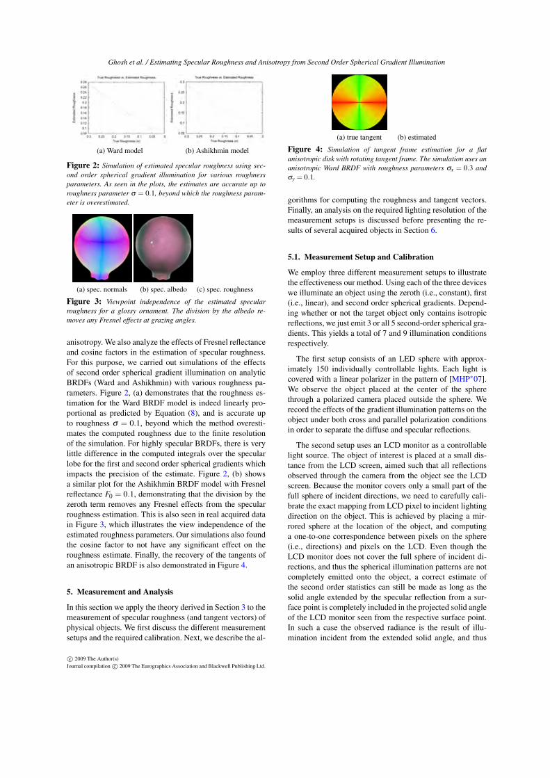
Figure 2: Simulation of estimated specular roughness using sec-ond order spherical gradient illumination for various roughnessparameters. As seen in the plots, the estimates are accurate up toroughness parameter σ = 0.1, beyond which the roughness param-eter is overestimated.

(a) spec. normals (b) spec. albedo (c) spec. roughness

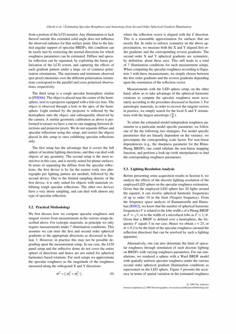
Figure 3: Viewpoint independence of the estimated specularroughness for a glossy ornament. The division by the albedo re-moves any Fresnel effects at grazing angles.

anisotropy. We also analyze the effects of Fresnel reflectanceand cosine factors in the estimation of specular roughness.For this purpose, we carried out simulations of the effectsof second order spherical gradient illumination on analyticBRDFs (Ward and Ashikhmin) with various roughness pa-rameters. Figure 2, (a) demonstrates that the roughness es-timation for the Ward BRDF model is indeed linearly pro-portional as predicted by Equation (8), and is accurate upto roughness σ = 0.1, beyond which the method overesti-mates the computed roughness due to the finite resolutionof the simulation. For highly specular BRDFs, there is verylittle difference in the computed integrals over the specularlobe for the first and second order spherical gradients whichimpacts the precision of the estimate. Figure 2, (b) showsa similar plot for the Ashikhmin BRDF model with Fresnelreflectance F0 = 0.1, demonstrating that the division by thezeroth term removes any Fresnel effects from the specularroughness estimation. This is also seen in real acquired datain Figure 3, which illustrates the view independence of theestimated roughness parameters. Our simulations also foundthe cosine factor to not have any significant effect on theroughness estimate. Finally, the recovery of the tangents ofan anisotropic BRDF is also demonstrated in Figure 4.

5. Measurement and Analysis

In this section we apply the theory derived in Section 3 to themeasurement of specular roughness (and tangent vectors) ofphysical objects. We first discuss the different measurementsetups and the required calibration. Next, we describe the al-

(a) true tangent (b) estimated

Figure 4: Simulation of tangent frame estimation for a flatanisotropic disk with rotating tangent frame. The simulation uses ananisotropic Ward BRDF with roughness parameters σx = 0.3 andσy = 0.1.

gorithms for computing the roughness and tangent vectors.Finally, an analysis on the required lighting resolution of themeasurement setups is discussed before presenting the re-sults of several acquired objects in Section 6.

5.1. Measurement Setup and Calibration

We employ three different measurement setups to illustratethe effectiveness our method. Using each of the three deviceswe illuminate an object using the zeroth (i.e., constant), first(i.e., linear), and second order spherical gradients. Depend-ing whether or not the target object only contains isotropicreflections, we just emit 3 or all 5 second-order spherical gra-dients. This yields a total of 7 and 9 illumination conditionsrespectively.

The first setup consists of an LED sphere with approx-imately 150 individually controllable lights. Each light iscovered with a linear polarizer in the pattern of [MHP∗07].We observe the object placed at the center of the spherethrough a polarized camera placed outside the sphere. Werecord the effects of the gradient illumination patterns on theobject under both cross and parallel polarization conditionsin order to separate the diffuse and specular reflections.

The second setup uses an LCD monitor as a controllablelight source. The object of interest is placed at a small dis-tance from the LCD screen, aimed such that all reflectionsobserved through the camera from the object see the LCDscreen. Because the monitor covers only a small part of thefull sphere of incident directions, we need to carefully cali-brate the exact mapping from LCD pixel to incident lightingdirection on the object. This is achieved by placing a mir-rored sphere at the location of the object, and computinga one-to-one correspondence between pixels on the sphere(i.e., directions) and pixels on the LCD. Even though theLCD monitor does not cover the full sphere of incident di-rections, and thus the spherical illumination patterns are notcompletely emitted onto the object, a correct estimate ofthe second order statistics can still be made as long as thesolid angle extended by the specular reflection from a sur-face point is completely included in the projected solid angleof the LCD monitor seen from the respective surface point.In such a case the observed radiance is the result of illu-mination incident from the extended solid angle, and thus

c 2009 The Author(s)Journal compilation c 2009 The Eurographics Association and Blackwell Publishing Ltd.

Ghosh et al. / Estimating Specular Roughness and Anisotropy from Second Order Spherical Gradient Illumination

from a portion of the LCD monitor. Any illumination or lackthereof outside this extended solid angle does not influencethe observed radiance for that surface point. Due to the lim-ited angular support of specular BRDFs, this condition canbe easily met by restricting the normal directions for whichroughness parameters can be estimated. Diffuse and specu-lar reflection can be separated, by exploiting the linear po-larization of the LCD screen, and capturing the effects ofeach gradient pattern under a large set of (camera) polar-ization orientations. The maximum and minimum observed(per-pixel) intensities over the different polarization orienta-tions correspond to the parallel and cross polarized observa-tions, respectively.

The third setup is a rough specular hemisphere similarto [PHD06]. The object is placed near the center of the hemi-sphere, next to a projector equipped with a fish-eye lens. Theobject is observed through a hole in the apex of the hemi-sphere. Light emitted by the projector is reflected by thehemisphere onto the object, and subsequently observed bythe camera. A similar geometric calibration as above is per-formed to ensure we have a one-to-one mapping between di-rections and projector pixels. We do not separate diffuse andspecular reflections using this setup, and restrict the objectsplaced in this setup to ones exhibiting specular reflectionsonly.

The first setup has the advantage that it covers the fullsphere of incident lighting directions, and thus can deal withobjects of any geometry. The second setup is the most re-strictive in this case, and is mostly suited for planar surfaces.In terms of separating the diffuse from the specular reflec-tions, the first device is by far the easiest (only two pho-tographs per lighting pattern are needed), followed by thesecond device. Due to the limited sampling density of thefirst device, it is only suited for objects with materials ex-hibiting rough specular reflections. The other two deviceshave a very dense sampling, and can deal with almost anytype of specular reflection.

5.2. Practical Methodology

We first discuss how we compute specular roughness andtangent vectors from measurements in the various setups de-scribed above. For isotropic materials, in principle we onlyrequire measurements under 7 illumination conditions. Thisassumes we can steer the first and second order sphericalgradients to the appropriate directions as discussed in Sec-tion 3. However, in practice this may not be possible de-pending upon the measurement setup. In our case, the LCDpanel setup and the reflective dome do not cover the entiresphere of directions and hence are not suited for sphericalharmonics based rotations. For such setups we approximatethe specular roughness as the magnitude of the roughnessmeasured along the orthogonal X and Y directions:

σ2 = σ2x +σ2

y , (9)

where the reflection vector is aligned with the Z direction.This is a reasonable approximation for surfaces that aremostly flat. In order to enforce symmetry on the above ap-proximation, we measure both the X and Y aligned first or-der gradients and the corresponding reverse gradients. Thesecond order X and Y spherical gradients are symmetric,by definition, about these axes. This still leads to a totalof 7 illumination conditions for such measurement setups.When computing the specular roughness according to Equa-tion 3 with these measurements, we simply choose betweenthe first order gradients and the reverse gradients dependingupon the orientation of the reflection vector.

Measurements with the LED sphere setup, on the otherhand, allow us to take advantage of the spherical harmonicrotations to compute the specular roughness more accu-rately according to the procedure discussed in Section 3. Foranisotropic materials, in order to recover the tangent vectorsin practice, we simply search for the local X and Y orienta-tions with the largest anisotropy ( σx

σy).

To relate the estimated model-independent roughness pa-rameter to a particular model specific parameter, we followone of the the following two strategies. For model specificparameters that are linearly dependent on the variance, weprecompute the corresponding scale factor. For non-lineardependencies (e.g., the sharpness parameter for the Blinn-Phong BRDF), one could tabulate the non-linear mappingfunction, and perform a look-up (with interpolation) to findthe corresponding roughness parameters.

5.3. Lighting Resolution Analysis

Before presenting some acquisition results in Section 6, weanalyze the effects of the discrete lighting resolution of theemployed LED sphere on the specular roughness estimation.Given that the employed LED sphere has 20 lights aroundthe equator, it can resolve spherical harmonic frequenciesof up to order 10 in the limit (Nyquist frequency). Fromthe frequency space analysis of Ramamoorthi and Hanra-han [RH02], we know that the number of spherical harmonicfrequencies F is related to the lobe width s of a Phong BRDFas F ≈

√s, or to the width of a microfacet lobe as F ≈ 1/σ .

Given that a BRDF is defined over a hemisphere, the fre-quency F equals 5 in our case. Hence we obtain s ≈ 25, orσ ≈ 0.2 to be the limit of the specular roughness (around thereflection direction) that can be resolved by such a lightingapparatus.

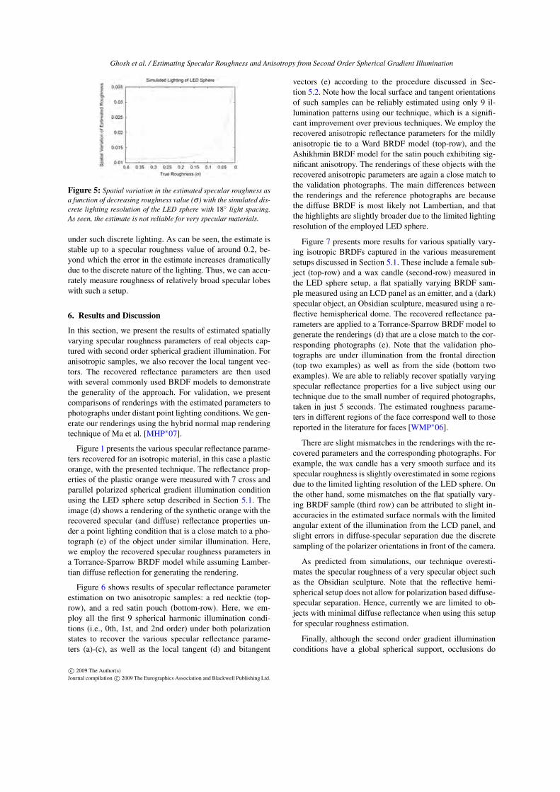
Alternatively, one can also determine the limit of specu-lar roughness through simulation of such discrete lightingon BRDFs with varying roughness parameters. For our sim-ulations, we rendered a sphere with a Ward BRDF modelwith spatially uniform specular roughness under the varioussecond order spherical gradient illumination conditions asrepresented on the LED sphere. Figure 5 presents the accu-racy in terms of spatial variation in the estimated roughness

c 2009 The Author(s)Journal compilation c 2009 The Eurographics Association and Blackwell Publishing Ltd.

Ghosh et al. / Estimating Specular Roughness and Anisotropy from Second Order Spherical Gradient Illumination

Figure 5: Spatial variation in the estimated specular roughness asa function of decreasing roughness value (σ ) with the simulated dis-crete lighting resolution of the LED sphere with 18 light spacing.As seen, the estimate is not reliable for very specular materials.

under such discrete lighting. As can be seen, the estimate isstable up to a specular roughness value of around 0.2, be-yond which the error in the estimate increases dramaticallydue to the discrete nature of the lighting. Thus, we can accu-rately measure roughness of relatively broad specular lobeswith such a setup.

6. Results and Discussion

In this section, we present the results of estimated spatiallyvarying specular roughness parameters of real objects cap-tured with second order spherical gradient illumination. Foranisotropic samples, we also recover the local tangent vec-tors. The recovered reflectance parameters are then usedwith several commonly used BRDF models to demonstratethe generality of the approach. For validation, we presentcomparisons of renderings with the estimated parameters tophotographs under distant point lighting conditions. We gen-erate our renderings using the hybrid normal map renderingtechnique of Ma et al. [MHP∗07].

Figure 1 presents the various specular reflectance parame-ters recovered for an isotropic material, in this case a plasticorange, with the presented technique. The reflectance prop-erties of the plastic orange were measured with 7 cross andparallel polarized spherical gradient illumination conditionusing the LED sphere setup described in Section 5.1. Theimage (d) shows a rendering of the synthetic orange with therecovered specular (and diffuse) reflectance properties un-der a point lighting condition that is a close match to a pho-tograph (e) of the object under similar illumination. Here,we employ the recovered specular roughness parameters ina Torrance-Sparrow BRDF model while assuming Lamber-tian diffuse reflection for generating the rendering.

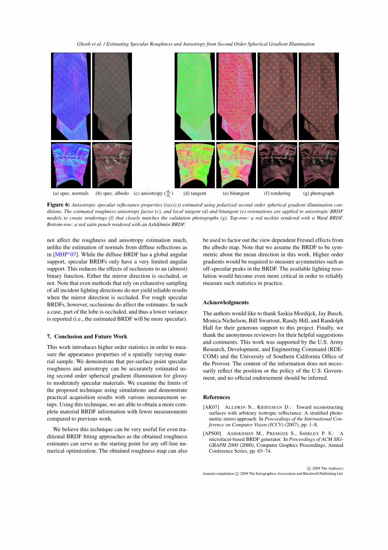
Figure 6 shows results of specular reflectance parameterestimation on two anisotropic samples: a red necktie (top-row), and a red satin pouch (bottom-row). Here, we em-ploy all the first 9 spherical harmonic illumination condi-tions (i.e., 0th, 1st, and 2nd order) under both polarizationstates to recover the various specular reflectance parame-ters (a)-(c), as well as the local tangent (d) and bitangent

vectors (e) according to the procedure discussed in Sec-tion 5.2. Note how the local surface and tangent orientationsof such samples can be reliably estimated using only 9 il-lumination patterns using our technique, which is a signifi-cant improvement over previous techniques. We employ therecovered anisotropic reflectance parameters for the mildlyanisotropic tie to a Ward BRDF model (top-row), and theAshikhmin BRDF model for the satin pouch exhibiting sig-nificant anisotropy. The renderings of these objects with therecovered anisotropic parameters are again a close match tothe validation photographs. The main differences betweenthe renderings and the reference photographs are becausethe diffuse BRDF is most likely not Lambertian, and thatthe highlights are slightly broader due to the limited lightingresolution of the employed LED sphere.

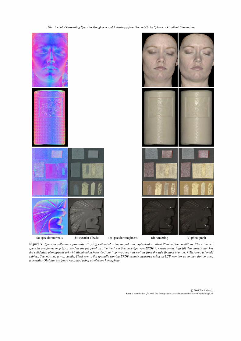
Figure 7 presents more results for various spatially vary-ing isotropic BRDFs captured in the various measurementsetups discussed in Section 5.1. These include a female sub-ject (top-row) and a wax candle (second-row) measured inthe LED sphere setup, a flat spatially varying BRDF sam-ple measured using an LCD panel as an emitter, and a (dark)specular object, an Obsidian sculpture, measured using a re-flective hemispherical dome. The recovered reflectance pa-rameters are applied to a Torrance-Sparrow BRDF model togenerate the renderings (d) that are a close match to the cor-responding photographs (e). Note that the validation pho-tographs are under illumination from the frontal direction(top two examples) as well as from the side (bottom twoexamples). We are able to reliably recover spatially varyingspecular reflectance properties for a live subject using ourtechnique due to the small number of required photographs,taken in just 5 seconds. The estimated roughness parame-ters in different regions of the face correspond well to thosereported in the literature for faces [WMP∗06].

There are slight mismatches in the renderings with the re-covered parameters and the corresponding photographs. Forexample, the wax candle has a very smooth surface and itsspecular roughness is slightly overestimated in some regionsdue to the limited lighting resolution of the LED sphere. Onthe other hand, some mismatches on the flat spatially vary-ing BRDF sample (third row) can be attributed to slight in-accuracies in the estimated surface normals with the limitedangular extent of the illumination from the LCD panel, andslight errors in diffuse-specular separation due the discretesampling of the polarizer orientations in front of the camera.

As predicted from simulations, our technique overesti-mates the specular roughness of a very specular object suchas the Obsidian sculpture. Note that the reflective hemi-spherical setup does not allow for polarization based diffuse-specular separation. Hence, currently we are limited to ob-jects with minimal diffuse reflectance when using this setupfor specular roughness estimation.

Finally, although the second order gradient illuminationconditions have a global spherical support, occlusions do

c 2009 The Author(s)Journal compilation c 2009 The Eurographics Association and Blackwell Publishing Ltd.

Ghosh et al. / Estimating Specular Roughness and Anisotropy from Second Order Spherical Gradient Illumination

(a) spec. normals (b) spec. albedo (c) anisotropy ( σxσy

) (d) tangent (e) bitangent (f) rendering (g) photograph

Figure 6: Anisotropic specular reflectance properties ((a)-(c)) estimated using polarized second order spherical gradient illumination con-ditions. The estimated roughness anisotropy factor (c), and local tangent (d) and bitangent (e) orientations are applied to anisotropic BRDFmodels to create renderings (f) that closely matches the validation photographs (g). Top-row: a red necktie rendered with a Ward BRDF.Bottom-row: a red satin pouch rendered with an Ashikhmin BRDF.

not affect the roughness and anisotropy estimation much,unlike the estimation of normals from diffuse reflections asin [MHP∗07]. While the diffuse BRDF has a global angularsupport, specular BRDFs only have a very limited angularsupport. This reduces the effects of occlusions to an (almost)binary function. Either the mirror direction is occluded, ornot. Note that even methods that rely on exhaustive samplingof all incident lighting directions do not yield reliable resultswhen the mirror direction is occluded. For rough specularBRDFs, however, occlusions do affect the estimates. In sucha case, part of the lobe is occluded, and thus a lower varianceis reported (i.e., the estimated BRDF will be more specular).

7. Conclusion and Future Work

This work introduces higher order statistics in order to mea-sure the appearance properties of a spatially varying mate-rial sample. We demonstrate that per-surface point specularroughness and anisotropy can be accurately estimated us-ing second order spherical gradient illumination for glossyto moderately specular materials. We examine the limits ofthe proposed technique using simulations and demonstratepractical acquisition results with various measurement se-tups. Using this technique, we are able to obtain a more com-plete material BRDF information with fewer measurementscompared to previous work.

We believe this technique can be very useful for even tra-ditional BRDF fitting approaches as the obtained roughnessestimates can serve as the starting point for any off-line nu-merical optimization. The obtained roughness map can also

be used to factor out the view dependent Fresnel effects fromthe albedo map. Note that we assume the BRDF to be sym-metric about the mean direction in this work. Higher ordergradients would be required to measure asymmetries such asoff-specular peaks in the BRDF. The available lighting reso-lution would become even more critical in order to reliablymeasure such statistics in practice.

Acknowledgments

The authors would like to thank Saskia Mordijck, Jay Busch,Monica Nichelson, Bill Swartout, Randy Hill, and RandolphHall for their generous support to this project. Finally, wethank the anonymous reviewers for their helpful suggestionsand comments. This work was supported by the U.S. ArmyResearch, Development, and Engineering Command (RDE-COM) and the University of Southern California Office ofthe Provost. The content of the information does not neces-sarily reflect the position or the policy of the U.S. Govern-ment, and no official endorsement should be inferred.

References[AK07] ALLDRIN N., KRIEGMAN D.: Toward reconstructing

surfaces with arbitrary isotropic reflectance: A stratified photo-metric stereo approach. In Proceedings of the International Con-ference on Computer Vision (ICCV) (2007), pp. 1–8.

[APS00] ASHIKHMIN M., PREMOZE S., SHIRLEY P. S.: Amicrofacet-based BRDF generator. In Proceedings of ACM SIG-GRAPH 2000 (2000), Computer Graphics Proceedings, AnnualConference Series, pp. 65–74.

c 2009 The Author(s)Journal compilation c 2009 The Eurographics Association and Blackwell Publishing Ltd.

Ghosh et al. / Estimating Specular Roughness and Anisotropy from Second Order Spherical Gradient Illumination

[Ash06] ASHIKHMIN M.: Distribution-based BRDFs, 2006.http://jesper.kalliope.org/blog/library/dbrdfs.pdf.

[AZK08] ALLDRIN N., ZICKLER T., KRIEGMAN D.: Photomet-ric stereo with non-parametric and spatially-varying reflectance.In Proceedings of IEEE Computer Vision and Pattern Recogni-tion (CVPR) (2008).

[FCM∗08] FRANCKEN Y., CUYPERS T., MERTENS T., GIELISJ., BEKAERT P.: High quality mesostructure acquisition usingspecularities. Computer Vision and Pattern Recognition, 2008.CVPR 2008. IEEE Conference on (2008), 1–7.

[GCHS05] GOLDMAN D. B., CURLESS B., HERTZMANN A.,SEITZ S. M.: Shape and spatially-varying brdfs from photomet-ric stereo. In ICCV ’05: Proceedings of the Tenth IEEE Inter-national Conference on Computer Vision (ICCV’05) Volume 1(2005), pp. 341–348.

[Geo03] GEORGHIADES A.: Recovering 3-D shape and re-flectance from a small number of photographs. In RenderingTechniques (2003), pp. 230U–240.

[GTHD03] GARDNER A., TCHOU C., HAWKINS T., DEBEVECP.: Linear light source reflectometry. In ACM SIGGRAPH 2003(2003), pp. 749–758.

[HLHZ08] HOLROYD M., LAWRENCE J., HUMPHREYS G.,ZICKLER T.: A photometric approach for estimating normalsand tangents. In SIGGRAPH Asia ’08: ACM SIGGRAPH Asia2008 papers (2008), pp. 1–9.

[HS03] HERTZMANN A., SEITZ S.: Shape and materials by ex-ample: a photometric stereo approach. Computer Vision and Pat-tern Recognition, 2003. Proceedings. 2003 IEEE Computer So-ciety Conference on 1 (2003), 533–540, vol.1.

[HTSG91] HE X. D., TORRANCE K. E., SILLION F. X.,GREENBERG D. P.: A comprehensive physical model for lightreflection. SIGGRAPH Comput. Graph. 25, 4 (1991), 175–186.

[LBAD∗06] LAWRENCE J., BEN-ARTZI A., DECORO C., MA-TUSIK W., PFISTER H., RAMAMOORTHI R., RUSINKIEWICZS.: Inverse shade trees for non-parametric material representa-tion and editing. ACM Transactions on Graphics 25, 3 (2006),735–745.

[LFTG97] LAFORTUNE E. P. F., FOO S.-C., TORRANCE K. E.,GREENBERG D. P.: Non-linear approximation of reflectancefunctions. In SIGGRAPH ’97: Proceedings of the 24th annualconference on Computer graphics and interactive techniques(1997), pp. 117–126.

[LGK∗01] LENSCH H. P. A., GOESELE M., KAUTZ J., HEI-DRICH W., SEIDEL H.-P.: Image-based reconstruction of spa-tially varying materials. In Proceedings of the 12th EurographicsWorkshop on Rendering Techniques (2001), pp. 103–114.

[LKG∗03] LENSCH H. P. A., KAUTZ J., GOESELE M., HEI-DRICH W., SEIDEL H.-P.: Image-based reconstruction of spatialappearance and geometric detail. ACM Transactions on Graphics22, 2 (2003), 234–257.

[Mar98] MARSCHNER S.: Inverse Rendering for ComputerGraphics. PhD thesis, Cornell University, 1998.

[MHP∗07] MA W.-C., HAWKINS T., PEERS P., CHABERT C.-F., WEISS M., DEBEVEC P.: Rapid acquisition of specular anddiffuse normal maps from polarized spherical gradient illumina-tion. In Rendering Techniques (2007), pp. 183–194.

[MZKB05] MALLICK S. P., ZICKLER T. E., KRIEGMAN D. J.,BELHUMEUR P. N.: Beyond lambert: Reconstructing specularsurfaces using color. In Proc. IEEE Conf. Computer Vision andPattern Recognition (2005).

[NDM05] NGAN A., DURAND F., MATUSIK W.: Experimen-tal analysis of brdf models. In Proceedings of the EurographicsSymposium on Rendering (2005), pp. 117–226.

[NRH∗77] NICODEMUS F. E., RICHMOND J. C., HSIA J. J.,GINSBERG I. W., LIMPERIS T.: Geometric considerations andnomenclature for reflectance. National Bureau of StandardsMonograph 160 (1977).

[PHD06] PEERS P., HAWKINS T., DEBEVEC P.: A ReflectiveLight Stage. Tech. Rep. ICT Technical Report ICT-TR-04.2006,ICT-USC, 2006.

[RH02] RAMAMOORTHI R., HANRAHAN P.: Frequency spaceenvironment map rendering. In Proc. of ACM SIGGRAPH ’02(2002), pp. 517–526.

[SKS02] SLOAN P.-P., KAUTZ J., SNYDER J.: Precomputedradiance transfer for real-time rendering in dynamic, low-frequency lighting environments. In SIGGRAPH ’02: Proceed-ings of the 29th annual conference on Computer graphics andinteractive techniques (2002), pp. 527–536.

[TS67] TORRANCE K. E., SPARROW E. M.: Theory of off-specular reflection from roughened surfaces. J. Opt. Soc. Am.57 (1967), 1104–1114.

[War92] WARD G. J.: Measuring and modeling anisotropic re-flection. SIGGRAPH Comput. Graph. 26, 2 (1992), 265–272.

[WMP∗06] WEYRICH T., MATUSIK W., PFISTER H., BICKELB., DONNER C., TU C., MCANDLESS J., LEE J., NGAN A.,JENSEN H. W., GROSS M.: Analysis of human faces using ameasurement-based skin reflectance model. ACM Transactionson Graphics 25, 3 (2006), 1013–1024.

[Woo78] WOODHAM R. J.: Photometric stereo: A reflectancemap technique for determining surface orientation from imageintensity. In Proc. SPIE’s 22nd Annual Technical Symposium(1978), vol. 155.

[ZBK02] ZICKLER T. E., BELHUMEUR P. N., KRIEGMAN D. J.:Helmholtz stereopsis: Exploiting reciprocity for surface recon-struction. Int. J. Comput. Vision 49, 2-3 (2002), 215–227.

[ZREB06] ZICKLER T., RAMAMOORTHI R., ENRIQUE S., BEL-HUMEUR P. N.: Reflectance sharing: Predicting appearance froma sparse set of images of a known shape. IEEE Trans. PatternAnal. Mach. Intell. 28, 8 (2006), 1287–1302.

c 2009 The Author(s)Journal compilation c 2009 The Eurographics Association and Blackwell Publishing Ltd.

Ghosh et al. / Estimating Specular Roughness and Anisotropy from Second Order Spherical Gradient Illumination

(a) specular normals (b) specular albedo (c) specular roughness (d) rendering (e) photograph

Figure 7: Specular reflectance properties ((a)-(c)) estimated using second order spherical gradient illumination conditions. The estimatedspecular roughness map (c) is used as the per pixel distribution for a Torrance-Sparrow BRDF to create renderings (d) that closely matchesthe validation photographs (e) with illumination from the front (top two rows), as well as from the side (bottom two rows). Top-row: a femalesubject. Second-row: a wax candle. Third row: a flat spatially varying BRDF sample measured using an LCD monitor as emitter. Bottom row:a specular Obsidian sculpture measured using a reflective hemisphere.

c 2009 The Author(s)Journal compilation c 2009 The Eurographics Association and Blackwell Publishing Ltd.