1

Department of Economics

Issn 1441-5429

Discussion paper 46/10

Estimating Residential Water Demand using the Stone-Geary Functional Form: the Case of Sri Lanka*

  Dinusha Dharmaratna and Edwyna Harris 

Abstract

This paper formulates a demand model for residential water in Sri Lanka using the Stone-Geary functional form. This functional form has two main advantages when compared with Cobb-Douglas: non-constant price elasticities and; it considers water consumption as two components – a fixed and a residual. These two components allow us to estimate the threshold below which water consumption is non-responsive to price changes. Our findings show that the portion of water use insensitive to price changes in Sri Lanka is between 0.64 and 1.06 per capita per month. This is below estimates for developed countries indicating that reducing water consumption via price instruments may be more successful in developing countries. Price elasticity ranges from -0.11 to -0.14 and the income elasticity varies from 0.11 to 0.14. These estimates are similar to those for developed countries suggesting policy makers should not rely solely on price instruments to reduce water consumption.

Key words: Stone-Geary, water demand, water pricing, block pricing, Sri Lanka

JEL Code: Q21, Q25 and C23

* Corresponding Author: Edwyna Harris, edwyna.harris@buseco.monash.edu.au, Telephone : +61 3 9905 2448; Fax : +61 9905 5476. This paper has benefitted from the valuable suggestions of Yew-Kwang Ng, Robert Brooks, and Jaai Parasnis. We also thank seminar participants at the HDR colloquium at Deakin University, Asia Pacific Week 2008 at Australian National University, the 2008 Australian Conference of Economists, and PhD conference of Business and Economics at Australian National University for comments on earlier drafts. © 2010 Dinusha Dharmaratna and Edwyna Harris All rights reserved. No part of this paper may be reproduced in any form, or stored in a retrieval system, without the prior written permission of the author.

2

Estimating residential water demand using the Stone-Geary functional form: the

case of Sri Lanka

1. Introduction

Many developed and developing countries are facing significant constraints on water

supplies that will continue over the coming decades in light of projected climate

change impacts. Growing populations and lack of available cost effective supply

augmentation options make reliable estimates of residential water demand important

for policy making. This is particularly true given the debate around whether policies

aimed at reducing water consumption should use price or non-price methods. In order

to determine whether demand is elastic or inelastic the standard literature primarily

uses the Cobb-Douglas function (for example: [7; 18; 23]). Estimates are typically in

the range of -0.25 and -0.75 (for example: [10; 12; 20; 29]). Higher elasticity

estimates are found only with long-run analysis and data restricted to summer

observations [2; 20; 21; 34; 40]. Several factors contribute to the weak sensitivity of

water consumption to price changes identified in empirical literature: 1) the intrinsic

nature of water as a necessity to life; 2) water bills constitute a small proportion of

overall household budget and; 3) imperfect price information [19].

However, water demand will exhibit different elasticities at different levels of use and

in different price ranges [34]. Moreover, the water volume required for the

necessities of life, such as drinking and cooking, will be extremely inelastic. For this

reason, the Stone-Geary functional form has two main advantages over Cobb-

Douglas: 1) it allows for non-constant price elasticities and; 2) it considers that water

consumption includes two components: a fixed quantity that cannot be adjusted

3

immediately after a price increase and a residual that can adapt instantaneously. This

allows us to establish a minimum water use threshold below which water

consumption is insensitive to price changes. Moreover, while Stone-Geary has been

used widely to analyse private consumption patterns for food, energy, transportation,

and labour, only three studies apply it to the water sector [3; 20; 34]. All three of

these studies have used data from developed countries. This paper adds to the

existing literature by using Stone-Geary but we use data from a developing nation, Sri

Lanka. Thus, the contribution is two-fold: 1) estimating threshold consumption for a

developing nation allows us to determine if these are likely to differ across nations at

various levels of development and; 2) enhance the debate surrounding the usefulness

of price compared with non-price methods to reduce water consumption.1

Our findings show price elasticity estimates range from -0.11 to -0.14. This illustrates

that while price inelastic in nature, water price increases may lead to some changes in

water consumption patterns. If such changes take place, price increases may

ultimately promote water conservation. However, our income elasticity estimate

range from 0.11 to 0.14. In a developing nation setting where incomes are expected

to rise over time this results leads use to expect increases in water consumption will

be experienced even if prices rise. Therefore, in an environment of increasing

incomes policy makers should not rely solely on prices to lower consumption levels.

Rather, they should employ a mix of instruments to effect reductions.

The minimum consumption threshold in Sri Lanka is between 2.7 and 4.5 cubic

metres per household per month. If we take the average household in Sri Lanka 1 Due to limited data availability we cannot compare the impact of price and non-price conservation measures to quantify their impacts as was done in Martinez-Espineira and Nauges [35]. As such, we can only make qualitative evaluations.

4

(Table 3) as being comprised of 4.2 members, our threshold per capita per month is

between 0.64 and 1.06. This estimation is lower than other empirical studies that

suggest a range between 2.52 to 13.58 cubic metres per capita per month [3; 20; 34].

However, we expect our results are bias downward for two main reasons: 1) because

coverage of the current pipe-borne water system is limited to approximately 30% of

the population and; 2) the availability of substitutes for example, wells. No data is

available to suggest the extent of substitution between supply sources that may be

utilised by households and therefore, we are unable to account for these effects in our

analysis. Nevertheless, the upper bound of our threshold per household is similar to

the World Health Organisation [45] standards for subsistence level water use at 4 to 5

cubic metres per month for a five member household. Average monthly water

consumption in Sri Lanka is 17 cubic metres per household suggesting further price

increases may be effective in reducing consumption. The inelastic nature of water

consumption means that by increasing prices water authorities will raise revenue

critical to maintain infrastructure and reduce transmission losses, as well as avoid low

equilibrium traps. Price increases will have a negative impact on poor households but

the revenue raised could be targeted to increase pipe-borne water supply to these

groups. This would substantially improve their standard of living.

The remained of the paper is set out as follows: section 2 provides details of the data

being used here; section 3 presents the methodology and econometric techniques

applied. Section 4 discusses the results and section 5 offers some concluding remarks

as well as directions for future research.

5

2. Data

Sri-Lankan residential water consumers’ face non-linear pricing, and the same pricing

schedule is administered across all water utility districts. The pricing system consists

of two types of charges: fixed and volumetric. The volumetric charge is variable and

subjected to increasing block pricing with eight blocks. Under the increasing block

tariff system, consumers’ monthly water bills under different blocks can be

mathematically expressed as follows:

QqifFqMPqqMPqqMPqqMPqqMPqqMPqqMPqQMPB

qQqifFqMPqQMPBqQifFQMPB

≤++−+−+−+−+−+−+−=

≤<++−=≤<+=

711122233344

455566676788

2111122

111

]*)(*)(*)(*)(*)(*)(*)(*[

)1(]*)(*[

0]*[

L

where, iB is the monthly water bill of customer using Q units of water; iMP is the

marginal price )..........( 148 MPMPMP >>> ; iq is the break point of the price schedule

(i=1-8); and F is the monthly fixed charge.

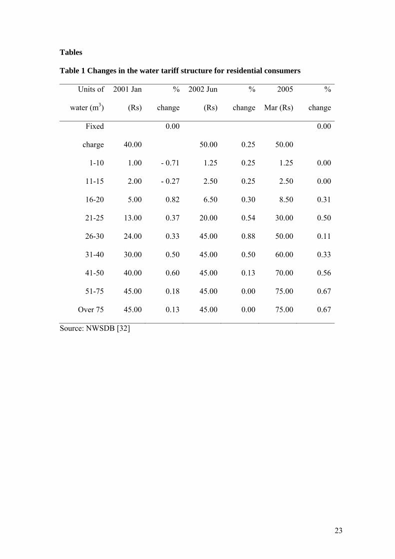
Table 1 shows the three price schedules during the 2001-05 time period considered

here. In 2001, the initial 10 cubic meters of water were charged at a rate of Sri Lankan

Rupees (SLRS) 1 per cubic meter.2 The charges increased gradually up to SLRS 40

per cubic meter when consumption exceeded 50 cubic meters. In mid-2002, prices in

all blocks were raised by SLRS 0.25 per cubic meter. Further revision of the price

structure was undertaken in 2005, without any changes to the rates of initial two

blocks. This price structure remains in operation today.

The National Water Supply and Drainage Board (NWSDB) is the principal authority

providing safe drinking water and sanitation in Sri Lanka. For administrative 2 According to Central Bank of Sri Lanka (16-05-2008), 1 USD = 108.15 SLRS

6

purposes, the NWSDB has divided Sri Lanka into six main regions and these support

centres independently administer their operation and maintenance budgets. The billing

and metering are decentralized to 14 district offices [1].3 Our data covers all 14

NWSDB districts over 60 months from January 2001 to December 2005, yielding a

total of 840 observations. Information on aggregate residential water consumption,

number of residential metered customers, and tariff structures for respective time

period were obtained from the NWSDB. We use panel data techniques to estimate

residential water demand in Sri Lanka. Panel data techniques have several advantages

over other methods [10; 20; 28]: 1) they are more informative; 2) they provide more

degrees of freedom and; 3) they can identify and measure effects that are simply not

detectable in cross-section or time series data.

The dependent variable, monthly average household water quantity is calculated by

dividing monthly total residential water quantity by total number of residential

connections for each district. Marginal price measures the changes in the price of the

final units of water purchased by the consumer and was calculated for each district

and month from the rate schedules for the relevant period and the average water

quantity. Assuming people purchase lower volumes of water as price increases, the

expected sign is negative. Marginal price corresponds to Taylor-Nordin specification

for increasing block tariff structures [38; 44]. It is an instrumented marginal price

derived by an artificial linearization of the theoretical water bills [9; 34].4

This approach has several advantages: 1) substitution of the estimated values of MP*

and D* into the demand equation frees the model from any asymptotic covariance 3 NWSDB districts are different to usual administrative districts in Sri Lanka, though the names are the same (refer Table 2). 4 More details of the instrumental marginal price are given in Appendix 1

7

between these two explanatory variables and error structure [16]; 2) any simultaneity

resulting from quantity dependent price is eliminated by using a marginal price that is

constant for all households subject to the same price schedule and; 3) instrumental

marginal price varies only over the rate structure and not over quantities consumed,

thus no feedback of quantity on price can occur.

To overcome concerns of the measurement problem of quantity that could be biasing

the instruments of MP and D , we use aggregate data [39]. Aggregate data are

generally less sensitive to outliers and measurement errors compared to specifications

based on observations corresponding to individual users and billing periods [31].

However, there are no problems arising from errors in the measurement of quantity

because the marginal price instrument does not vary with quantity thus making it

impossible to assign a wrong marginal price ex-post from the rate schedule.

Moreover, aggregate data can also be used but the results may be biased unless

aggregate marginal price and the difference variables are weighted by the proportion

of households actually consuming in each block. Unfortunately, this requires

information beyond which is available for this study and the data on distribution of

users among blocks are not available from the NWSDB.

Price is not the only factor determining household water consumption. The quantity of

water consumed also depends on additional factors including household income,

number of household members, and weather variables [4; 14; 42]. Socio-economic

variables were obtained from two sources: the Department of Census and Statistics,

2001/02 and 2005/06 Household Income and Expenditure Survey; and the Central

8

Bank of Sri Lanka’s 2003/04 Consumer Finances and Socio-economic Survey.

Interpolation was used to derive the monthly income and number of household

members for the intervening periods.

Income is one of the main determinants of consumption and this may act as a proxy

for water-using appliances. The income variable included in the analysis is monthly

virtual income, which is computed by adding average household income to the

instrument Nordin-difference variable. Instrumented Nordin-difference variable is

derived from the intercept of the estimated theoretical water bills to derive

instrumented marginal price variable.5 Average household income values for each

NWSDB district were obtained by weighting the incomes from administrative

districts. Empirical evidence suggests water demand is inelastic with respect to

income and small in magnitude [6; 12; 18; 20]. This is to be expected as water bills

often represent a small proportion of total household income [4]. Assuming water

consumption increases with the level of income, the expected sign on the derivative

with respect to income is positive.

Our model includes number of household members to capture household water

consumption decisions. Household size is expected to positively affect household

water use. However, due to economies of scale, the increase in water use is less than

proportional to the increase in household size [4; 24]. We expect our empirical results

will conform to past empirical studies so that water consumption will be positively

related to the number of household members. Age distribution within the household

members have varying impacts on residential water use [35]. Specifically, increasing

5 Procedure adopted to obtain instrumental marginal price and the instrumented difference variable is given in Appendix 1.

9

the number of adults compared to children will raise household water consumption,

whereas, more seniors will reduce consumption.

Weather data over the period were collected from the Sri Lankan Department of

Meteorology. Climatic effects in residential water demand models can be introduced

in different ways. For example, precipitation during the growing season [7; 8];

evapotranspiration from Bermuda grass minus rainfall [9; 23; 36] or; temperature with

annual or monthly rainfall [25; 43]. Generally, climate exerts the following

influences on water demand: high temperatures increase water demand while high

rainfalls decrease water demand. Outdoor water use depends on climatic conditions

that are represented by weather variables. To capture the influence of climate,

monthly and district average temperature and average rainfall data are used in the

demand estimation. The coefficient of temperature with respect to water use is

expected to be positive; while the coefficient of rainfall is expected to be negative.

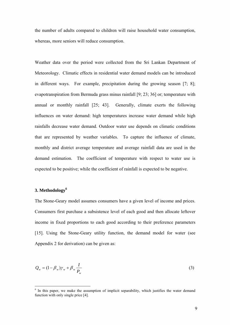
3. Methodology6

The Stone-Geary model assumes consumers have a given level of income and prices.

Consumers first purchase a subsistence level of each good and then allocate leftover

income in fixed proportions to each good according to their preference parameters

[15]. Using the Stone-Geary utility function, the demand model for water (see

Appendix 2 for derivation) can be given as:

 

)3()1(w

wwww PIQ βγβ +−=   

6 In this paper, we make the assumption of implicit separability, which justifies the water demand function with only single price [4].

10

 

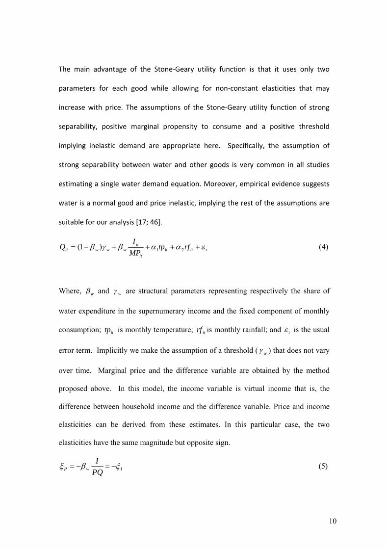
The main  advantage  of  the  Stone‐Geary  utility  function  is  that  it  uses  only  two 

parameters  for  each  good  while  allowing  for  non‐constant  elasticities  that  may 

increase with price. The  assumptions of  the  Stone‐Geary utility  function of  strong 

separability,  positive  marginal  propensity  to  consume  and  a  positive  threshold 

implying  inelastic  demand  are  appropriate  here.    Specifically,  the  assumption  of 

strong  separability between water  and other  goods  is  very  common  in  all  studies 

estimating a single water demand equation. Moreover, empirical evidence suggests 

water is a normal good and price inelastic, implying the rest of the assumptions are 

suitable for our analysis [17; 46].  

)4()1( 21 tititit

itwwwit rftp

MPI

Q εααβγβ ++++−=  

 

Where, wβ and wγ are structural parameters representing respectively the share of

water expenditure in the supernumerary income and the fixed component of monthly

consumption; ittp is monthly temperature; itrf is monthly rainfall; and tε is the usual

error term. Implicitly we make the assumption of a threshold ( wγ ) that does not vary

over time. Marginal price and the difference variable are obtained by the method

proposed above. In this model, the income variable is virtual income that is, the

difference between household income and the difference variable. Price and income

elasticities can be derived from these estimates. In this particular case, the two

elasticities have the same magnitude but opposite sign.

)5(IwP PQI ξβξ −=−=

11

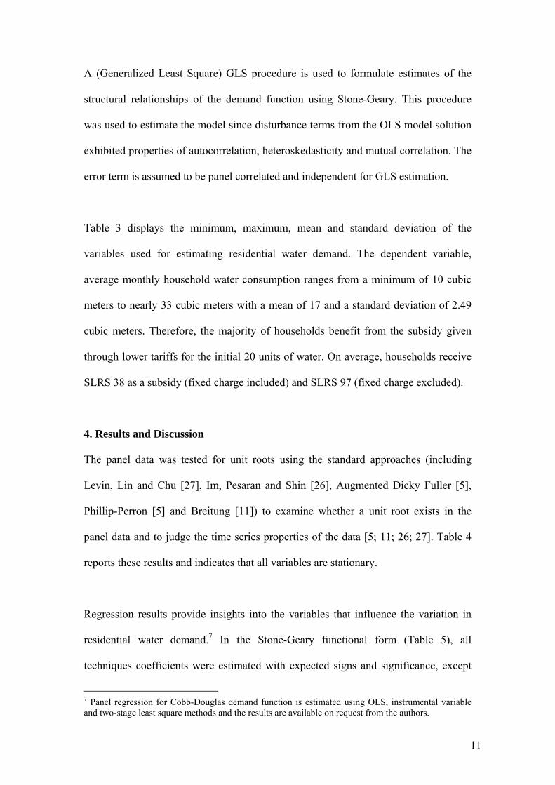
A (Generalized Least Square) GLS procedure is used to formulate estimates of the

structural relationships of the demand function using Stone-Geary. This procedure

was used to estimate the model since disturbance terms from the OLS model solution

exhibited properties of autocorrelation, heteroskedasticity and mutual correlation. The

error term is assumed to be panel correlated and independent for GLS estimation.

Table 3 displays the minimum, maximum, mean and standard deviation of the

variables used for estimating residential water demand. The dependent variable,

average monthly household water consumption ranges from a minimum of 10 cubic

meters to nearly 33 cubic meters with a mean of 17 and a standard deviation of 2.49

cubic meters. Therefore, the majority of households benefit from the subsidy given

through lower tariffs for the initial 20 units of water. On average, households receive

SLRS 38 as a subsidy (fixed charge included) and SLRS 97 (fixed charge excluded).

4. Results and Discussion

The panel data was tested for unit roots using the standard approaches (including

Levin, Lin and Chu [27], Im, Pesaran and Shin [26], Augmented Dicky Fuller [5],

Phillip-Perron [5] and Breitung [11]) to examine whether a unit root exists in the

panel data and to judge the time series properties of the data [5; 11; 26; 27]. Table 4

reports these results and indicates that all variables are stationary.

Regression results provide insights into the variables that influence the variation in

residential water demand.7 In the Stone-Geary functional form (Table 5), all

techniques coefficients were estimated with expected signs and significance, except

7 Panel regression for Cobb-Douglas demand function is estimated using OLS, instrumental variable and two-stage least square methods and the results are available on request from the authors.

12

for coefficient of rainfall with common AR(1) and panel specific AR(1) techniques.

The share of water expenses in the income wβ from equation (3) is small but

significantly different from zero. The low value of the wβ is not surprising because

the proportion of water expenses in overall household budget is low. Mean household

size contributes positively to water consumption but the respective coefficients are not

significant. The coefficient on the number of household members implies a one

percent increase in household size will increase household water consumption by 0.26

to 0.54 percent across different techniques.

In relation to climate, as expected, water consumption increases with temperature and

decreases with rainfall. Temperature is significant and has the expected positive sign

while the rainfall is not significant in common AR(1) and panel specific AR(1). The

coefficient of monthly temperature is relatively larger than the coefficient of monthly

rainfall. The small size of the estimated coefficient for monthly rainfall suggests

rainfall does not have a significant impact on water consumption decisions. The

coefficients imply that if monthly rainfall increases by 10 percent, monthly household

water consumption decreases approximately by 0.02 percent. A 10 percent rise in

monthly temperature will increase monthly residential water use by 3.1 to 3.7

percent.8

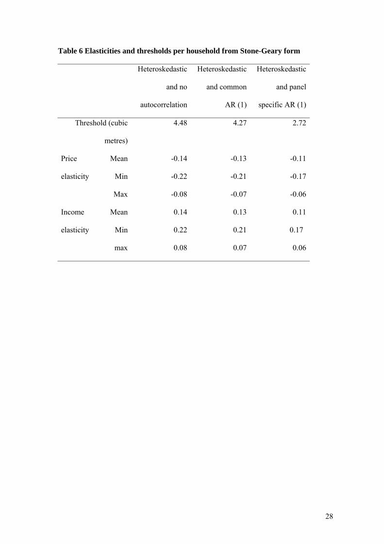
The threshold wγ from equation (3) is highly significant in the no autocorrelation

technique, estimated at 4.48 cubic meters per month per household. Across the

different estimation techniques, the threshold values range from 2.72 to 4.48 cubic

meters per month per household. Table 6 presents the value of threshold across 8 The coefficient of rainfall is 0.007 and the coefficient of temperature is 0.56 to 0.99 with the Cobb-Douglas estimations.

13

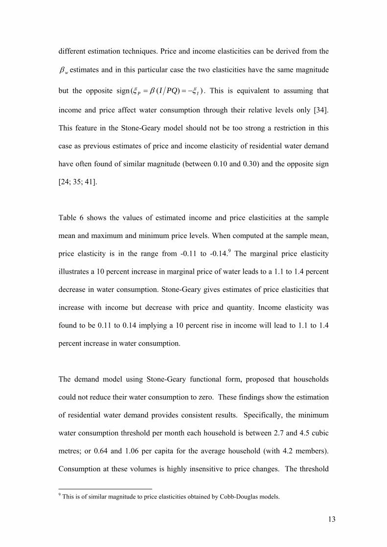
different estimation techniques. Price and income elasticities can be derived from the

wβ estimates and in this particular case the two elasticities have the same magnitude

but the opposite sign ))(( IP PQI ξβξ −== . This is equivalent to assuming that

income and price affect water consumption through their relative levels only [34].

This feature in the Stone-Geary model should not be too strong a restriction in this

case as previous estimates of price and income elasticity of residential water demand

have often found of similar magnitude (between 0.10 and 0.30) and the opposite sign

[24; 35; 41].

Table 6 shows the values of estimated income and price elasticities at the sample

mean and maximum and minimum price levels. When computed at the sample mean,

price elasticity is in the range from -0.11 to -0.14.9 The marginal price elasticity

illustrates a 10 percent increase in marginal price of water leads to a 1.1 to 1.4 percent

decrease in water consumption. Stone-Geary gives estimates of price elasticities that

increase with income but decrease with price and quantity. Income elasticity was

found to be 0.11 to 0.14 implying a 10 percent rise in income will lead to 1.1 to 1.4

percent increase in water consumption.

The demand model using Stone-Geary functional form, proposed that households

could not reduce their water consumption to zero. These findings show the estimation

of residential water demand provides consistent results. Specifically, the minimum

water consumption threshold per month each household is between 2.7 and 4.5 cubic

metres; or 0.64 and 1.06 per capita for the average household (with 4.2 members).

Consumption at these volumes is highly insensitive to price changes. The threshold

9 This is of similar magnitude to price elasticities obtained by Cobb-Douglas models.

14

level reported herein is conditional. It is conditional because the threshold is

dependent on available technology, pricing structure, and the price of water-

consuming durable goods [20].

The threshold range reported is lower than the three other studies that have employed

the Stone-Geary functional form utilising data from developed nations. Using data

from Seville, Spain [34] estimated a threshold of 4.7 cubic metres per capita per

month while [3], using data from Kuwait, estimated a threshold of 2.52 cubic meters

per capita per month. The third study, [20] estimated a significantly higher threshold

range of 12.09 to 13.58 cubic meters per capita per month. The main reason for such

large estimates in this latter study was water production rather than water

consumption was used [20] implying that all losses to the system were included in the

threshold. As a result, it would be logical to assume that study’s results lacked

accuracy. Our findings suggest a lower threshold than those of [34]; but are closer to

[3] estimates. This suggests there may be differences in threshold levels between

developed and developing nations. However, as noted, given the limited coverage of

pipe-borne water to the Sri Lankan population (approximately 30%) and the

availability of substitutes the differences between our threshold and these two studies

may simply be a function of data availability. Further application of Stone-Geary

using data from developing countries would provide a larger pool of results to

determine whether this is in fact the case across most developing nations.

Our results do provide water managers with important information about the threshold

of the quantity of water below which consumption will not respond to price changes.

Policies should explicitly recognize this in demand management efforts. Moreover,

15

even with a price inelastic nature, water price increases above the threshold may

promote reductions in water consumption patterns. If such a change takes place, then

increasing the price of water may ultimately promote water conservation. However,

because developing nations like Sri Lanka face increasing incomes, prices alone will

be unable to achieve significant water consumption reduction. In turn, the estimates

reported here suggest there may be little scope for significant consumption reduction

by simply relying on the price mechanism alone. In a developing nation setting this

provides an important guide for policy and what should be expected from price

changes in the residential water sector. Further, the results indicate policy makers

will need to use a mixture of instruments. Specifically, water price increases should

be accompanied by activities such as consumer awareness and education on water

leakage and wastage; investment on water efficient appliances; and the use of

recycled water outdoors.

5. Conclusion

This paper reports econometric results of residential water demand for pipe-borne

water in Sri Lanka, using monthly district data from January 2001 to December 2005.

Employing the Stone-Geary forms our estimates show price elasticity of water

demand ranges from 0.11 and -0.14.10 This is consistent with past findings for both

developed and developing countries [13; 17].

The results indicate the estimated coefficients are fairly stable over the different

techniques. However, the estimated coefficients on the difference variable across the

models suggest instability. The income elasticity is relatively small and significant,

10 For the Cobb-Douglas form, estimated price elasticity of water demand ranges from -0.06 to -0.58 and the income elasticities range from 0.03 to 0.13.

16

ranging from 0.11 to 0.14 for Stone-Geary functional forms. The income inelasticity

and smaller magnitude could be due to expenditure on water for residential

consumption comprising a very small proportion of the household budget.

The number of household members had a positive sign but was not significant with all

techniques. As expected, larger households consume more water for bathing, laundry,

toilet flushing and dish washing. Sizes of the coefficient are relatively larger and

range from 0.26 to 0.54, implying that water use changes are less than proportional to

the increase in household size.11 This is because of economies of scale in water usage

including cooking, cleaning, car washing and gardening. The analysis provides a

better approach to the investigation of climatic effects on water use by incorporating

monthly and district differences. Both coefficients of monthly temperature and

monthly rainfall are significant with expected signs.

The overall results suggest water consumption is not very responsive to price changes

in Sri Lanka and this finding may be applicable for other developing countries.

Moreover, the estimated price and income elasticities do not differ appreciably from

those of developed countries. Under inelastic response to price changes, pricing

policies have limited scope in changing water consumption.

The findings here suggest the importance of further research to apply the Stone-Geary

utility function to a larger number of developing countries to determine whether the

threshold consumption level varies appreciably across nations. This will have

important implications for policy design, particularly with regard to the effectiveness

11 The coefficient of the number of household varies from 0.21 to 0.86 for Cobb-Douglas form.

17

of using price to reduce consumption in these countries. Specifically, if the threshold

below which consumption is not responsive to price changes is appreciably lower for

developing nations than estimates for developed nations then using price as an

instrument to reduce consumption in the former may be more effective than in the

latter. However, it is important to recognise that the threshold level may be

underestimated in the developing country context given the limited coverage of pipe-

borne water connections that tends to persist in those nations. Further studies that

utilise developing country data will create better evidence as to whether this is in fact

the case. As a result, we would be better able to determine the effectiveness of price

compared with non-price instruments to effect consumption reductions in the water

sector. These studies are critically important for developing nation policy as

populations continue to increase and the expected effects of climate change become

more pronounced.

18

Appendix 1

Residential water demand model with marginal price and difference variable can be

expressed as follows:

Where, Q is monthly water consumption for an average household; MP is marginal

price for the last unit purchased; D is the difference between the actual water bill and

what would be paid if all units were purchased at MP ; W is a vector of weather

variables (temperature and rainfall) and Y is a vector of socio-economic variables

(household income and number of household members). The marginal price model

includes three structural equations because quantity, marginal price, and the

difference variable are simultaneously determined. The first model utilizes observed

quantity values and then is solved for MP and D. The values for MP and D are

then used in the demand equation.

Simultaneity arises because the quantity of water determines the price under the

pricing schedule. With block-rate pricing, causality goes in both directions, from price

to quantity and from quantity to price. Consumers choose the amount of water

depending on some measure of price, and the price paid depends on the amount

consumed. As a result, the Ordinary Least Square (OLS) assumption that

independence between the error term and the explanatory variables exists is violated

because water price depends on the quantity. This will yield biased and inconsistent

estimates [22].

), ( ), (

),,, (

structurerate Q f D structurerate Q f MP

YWD MPf Q

==

=

19

To overcome this, the instrumental variable approach has been used in similar studies

[9; 37]. Consistent parameters may be obtained by an instrumental variable method.

The objective of the instruments is to provide a proxy for the endogenous variables

that are price variables in water studies. The instrument should fulfil the requirement

of being uncorrelated with the error structure while being correlated with the

stochastic regressor [16].

Stone-Geary model uses an artificial linearization of the tariff structure to derive

instruments for marginal price and difference variable. This assumes that, instead of

taking the effort to learn how the tariff works and which block they are consuming in

at each moment in time, households will roughly estimate the whole tariff as a ray line

given by an intercept and a constant marginal price [29].

The total revenue )(TR function is computed using the range of quantity )(Q values

(10 – 33 cubic meters) encountered in the entire data set. These values of the total

revenue are then regressed against the corresponding quantity values. The first

derivative of the estimated function gives

*MP is the instrumental marginal price variable to the consumer and marginal

revenue to the water utility. Estimating the parameter α in equation 1 gives the

difference between what consumers actually pay and what consumers would pay if all

* MPq

TR =∂∂

=Λ β

QTR βα +=

20

units were sold at the marginal price *MP , that is the instrumental difference variable

*D . This procedure results in the representation of each rate schedule by *MP

and *D , which are constant for all observations under each specific rate structure.

Appendix 2: Stone-Geary functional form

Let wQ and zQ be demands for water and all other goods respectively, while wP and

zP are unit prices. wγ and zγ are minimum amounts (subsistence level) and wβ and

zβ are preference parameters (marginal budget shares) and I is income [34].

The Stone Geary utility function: )ln()ln( zzzwww QQU γβγβ −+−=

Where 0)(0)(,10,0 >−>−=+>> wwzzzwzw QandQ γγββββ

0)(0)(,10,0 >−>−=+>> wwzzzwzw QandQ γγββββ

Normalizing the price of the aggregate goods to one result following budget

constraint: zww QPQI +=

21

Maximizing utility subject to budget constraint yield the following demand

function

ww

zwwww

w

wwwwwwzww

zww

w

wzwwwzzzw

zww

zz

z

z

www

w

w

zwwzzzwww

PPI

QorP

PPIQ

QPQIinngsubstituti

QPQgAssu

QPQILQQ

L

PQQ

LQPQIQQL

γγγ

βγβγβγβ

ββγγβ

ββ

λ

λγ

β

λγ

βλγβγβ

+−−

=−+−

=

+=

+−==+

+=→∂∂

=−

→∂∂

=−

→∂∂

−−+−+−=

)(1min

)(

)(

)()ln()ln(

Preference parameter for water can be given as; zww

wwwww PI

PQPγγγβ−−

−=

It is assumed that 0=zγ , so the demand function for water is given as;

wwwww P

IQ βγβ +−= )1(

After assuming 0=zγ , wγ can be renamed as conditional water use threshold [20]

and is a threshold below which consumption is not affected by prices. The term

conditional emphasizes that this threshold is dependent on the available technology,

pricing structure and price of durable goods during the period of

estimation. wβ represents the marginal budget share allocated to water.

Income variable in this model is the virtual income and it is the difference between

household income and difference variable. Price and income elasticities can be

derived from these estimates. In this particular case, the two elasticities have the same

magnitude but opposite sign.

22

Iww

zwP QP

Iξ

γβξ −=

−−=

Following literature (for example, McGuire [30]; Gaudin et al.,[20]; Martinez-

Espineira and Nauges [34]) zγ is abstracted from the equation and the price elasticity

of water demand simplifies to

IwP PQI ξβξ −==

This simple specification is preferred since zγ does not provide any relevant

information to the study.

23

Tables

Table 1 Changes in the water tariff structure for residential consumers

Units of

water (m3)

2001 Jan

(Rs)

%

change

2002 Jun

(Rs)

%

change

2005

Mar (Rs)

%

change

Fixed

charge

40.00

0.00

50.00

0.25

50.00

0.00

1-10 1.00 - 0.71 1.25 0.25 1.25 0.00

11-15 2.00 - 0.27 2.50 0.25 2.50 0.00

16-20 5.00 0.82 6.50 0.30 8.50 0.31

21-25 13.00 0.37 20.00 0.54 30.00 0.50

26-30 24.00 0.33 45.00 0.88 50.00 0.11

31-40 30.00 0.50 45.00 0.50 60.00 0.33

41-50 40.00 0.60 45.00 0.13 70.00 0.56

51-75 45.00 0.18 45.00 0.00 75.00 0.67

Over 75 45.00 0.13 45.00 0.00 75.00 0.67

Source: NWSDB [32]

24

Table 2 Regional Support Centres and relevant districts

RSC NWSDB

Districts

Districts

Southern and Uva Galle Galle

Matara Matara

Hambantota Hambantota

Bandarawela Moneragala and Badulla

Western Kalutara Kalutara

Gampaha Gampaha

North Central and

North West

Kurunagala Kurunegala and Puttalam

Anuradhapura Anuradhapura and

Polonnaruwa

Central and

Sabaragamuwa

Kandy Kandy, Nuwara Eliya and

Matale

Ratnapura Ratnapura and Kegalle

North and East Trincomalee Trincomalee

Jaffna Mannar, Vavuniya,

Kilinochchi, Jaffna and

Mullativu

Ampara Ampara, Batticaloa

Greater Colombo Colombo Colombo

Source: NWSDB[33]

25

Table 3 Descriptive statistics

Variable Units Mean Std.

Dev.

Min Max

Monthly household water

demand

m3/month 17.06 2.49 9.65 33.21

Real marginal price Rs/m3 8.00 6.06 1.25 61.37

Real difference without fixed

charge

Rs 97.03 124.91 0.00 1338.17

Real difference with fixed

charge

Rs 37.99 125.29

57.78 1288.07

Real average price Rs/month 6.38 1.06 5.00 21.18

Number of residents in

household

persons 4.24 0.19241 3.72 4.80

Real mean income Rs/month 21301.72 6674.82 11143.80 44755.81

Real mean virtual income Rs/month 21640.25 6727.22 11347.22 45059.97

Monthly temperature 0C 27.23 2.17 18.90 31.70

Monthly rainfall mm 158.01 140.32 0.00 1337

Real instrumented marginal

price

Rs/m3 28.32 10.67 17.63 52.88

Real instrumented difference

variable with fixed charge

Rs 338.53 162.60 183.05 711.60

26

Table 4 Panel unit root test results

Variable Test for common

unit root process

Test for individual unit

root process

Natural log of water

quantity

LLC IPS, ADF-Fisher, PP-

Fisher

Natural log of real

marginal price

LLC IPS, ADF-Fisher, PP-

Fisher

Natural log of real

difference

LLC IPS, ADF-Fisher, PP-

Fisher

Natural log of real mean

income

LLC PP - Fisher

Natural log of real

household members

LLC, Breitung IPS, ADF-Fisher, PP-

Fisher

Natural log of temperature Breitung IPS, ADF-Fisher, PP-

Fisher

Natural log of rainfall LLC, Breitung IPS, ADF-Fisher, PP-

Fisher

Note: tests that reject the null hypothesis or non-stationarity are given in the table

where, LLC- Levin, Lin and Chu t*, Breitung- Breitung t-stat, IPS- Im, Pesaran and

Shin W-stat, ADF-Fisher Chi-square –Augmented Dicky Fuller and PP- Fisher Chi-

square – Phillip-Perron

27

Table 5 Water demand model estimates – Stone-Geary model

Heteroskedastic

and no

autocorrelation

Heteroskedastic

and common

AR (1)

Heteroskedastic

and panel

specific AR (1)

Constant 4.4686

(1.3584)***

4.2585

(2.2470)**

2.7169

(2.1068)

Income/price 0.0032

(0.0002)***

0.0029

(0.0003)***

0.0024

(0.0003)***

Household size 0.3889

(0.3184)

0.2599

(0.5267)

0.5403

(0.4793)

Rainfall -0.0018

(0.0004)***

-0.0002

(0.0003)

-0.0001

(0.0003)

Temperature 0.3127

(0.0195)***

0.3408

(0.0313)***

0.3649

(0.0302)***

Notes: *** Significant at α = 0.01, ** Significant at α = 0.05 and * Significant at α =

0.10 standard error values (robust) in parentheses below estimates, Dependant

variable is monthly water demand

28

Table 6 Elasticities and thresholds per household from Stone-Geary form

Heteroskedastic

and no

autocorrelation

Heteroskedastic

and common

AR (1)

Heteroskedastic

and panel

specific AR (1)

Threshold (cubic

metres)

4.48 4.27 2.72

Price

elasticity

Mean -0.14 -0.13 -0.11

Min -0.22 -0.21 -0.17

Max -0.08 -0.07 -0.06

Income

elasticity

Mean 0.14 0.13 0.11

Min 0.22 0.21 0.17

max 0.08 0.07 0.06

29

References

[1] ADB. Sri Lanka Country Assistance Program Evaluation: Water Supply and

Sanitation Sector Assistance Evaluation, Operations Evaluation Department,

Asian Development Bank (2007).

[2] D. Agthe, B. Billings, J. Dobra, and K. Raffiee, A Simultaneous Equation

Model for Block Rates. Water Resources Res. (1986) 1 - 4.

[3] M. Al-Quanibet, and R. Johnston, Municipal Demand for Water in Kuwait:

Methodological Issues and Empirical results. Water Resources Res. 21 (1985)

433 - 438.

[4] F. Arbues, M. Garcia-Valinas, and R. Martinez-Espineira, Estimation of

Residential Water Demand: A State-of-the-art-review. J. Socio-Econ. 32

(2003) 81 - 102.

[5] B.H. Baltagi, and C. Kao, Nonstationary Panels, Cointegration in Panels and

Dynamic Panels: A Survey. Advances in Econometrics 15 (2000) 7 - 51.

[6] N. Barkatullah, Pricing, Demand Analysis and Simulation: An Application to

a Water Utility, Dissertation.com, 1999.

[7] B. Beattie, and H. Foster, on the specification of price in studies of consumer

demand under block price scheduling. Land Econ. 57 (1981) 624 - 629.

[8] B. Beattie, and H. Foster, Urban Residential Demand for Water in the United

States. Land Econ. 55 (1979) 43 - 58.

[9] B. Billings, Specification of Block Rate Price Variables in Demand Models.

Land Econ. 58 (1982) 386 - 393.

[10] B. Billings, and D. Agthe, Price Elasticity for Water: A Case of Increasing

Block Rates. Land Econ. 56 (1980) 73 - 85.

30

[11] J. Breitung, The Local Power of Some Unit Root Tests for Panel Data.

Advances in Econometrics 15 (2000) 161 - 178.

[12] D. Chicoine, and G. Ramamurthy, Evidence in the Specification of Price in the

Study of Domestic Water Demand. Land Econ. 62 (1986) 26 - 32.

[13] J.M. Dalhuisen, R.J. Florax, H. De-Groot, and P. Nijkamp, Price and Income

Elasticities of Residential Water Demand: A Meta Analysis. Land Econ. 79

(2003) 292 - 308.

[14] C.C. David, and A.B. Inocencio, Understanding Household Demand for

Water: The Metro Manila Case, EEPSEA (1998).

[15] A. Deaton, and J. Muellbauer, Economics and Consumer Behaviour,

Cambridge University Press, Cambridge (1980).

[16] S. Deller, D. Chicooine, and G. Ramamurthy, Instrumental Variables

Approach to Rural Water Service Demand. Southern Econ. J. 53 (1986) 333 -

346.

[17] M. Espey, J. Espey, and W.D. Shaw, Price Elasticity of Residential Demand

for Water: A Meta-analysis. Water Resources Res. 33 (1997) 1369 - 1374.

[18] S. Garcia, and A. Reynaud, Estimating Benefits of Efficient Water Pricing in

France. Resource Energy Econ. 26 (2004) 1 - 25.

[19] S. Gaudin, Effect of price information on residential water demand. Applied

Econ. 38 (2006) 383 - 393.

[20] S. Gaudin, R. Griffin, and R. Sickles, Demand Specification for Municipal

Water Management: Evaluation of the Stone-Geary Form. Land Econ. 77

(2001) 399 - 422.

31

[21] W.M. Hanemann, Price Rate and Structures. in Urban Water Demand

Management and Planning, (D.D. Baumann, J.J. Boland and W.M. Hanemann,

Ed.), McGraw-Hill, New York. (1997)

[22] S. Hensen, Electricity Demand Estimates Under Increasing Block Rates.

Southern Econ. J. (1984) 147 - 156.

[23] J.A. Hewitt, and W.M. Hanemann, A discrete/continuous choice approach to

residential water demand under block rate pricing Land Econ. 71 (1995) 173 -

192.

[24] L. Hoglund, Household Demand for Water in Sweden with Implications of

Potential Tax on Water Use. Water Resources Res. 35 (1999) 3853 - 3863.

[25] I. Hussain, S. Thrikawala, and R. Barker, Economic Analysis of Residential,

Commercial and Industrial Uses of Water in Sri Lanka. Water Int. 27 (2002)

183 - 193.

[26] K.S. Im, and M.H. Pesaran, On the Panel Unit Root Tests using Nonlinear

Instrumental Variables, Cambridge Working Papers in Economics, University

of Cambridge (2003).

[27] A. Levin, C.F. Lin, and J. Chu, Unit Root Test in Panel Data: Asymptotic and

Finite Sample Properties. J. Econometrics 108 (2002) 1 - 24.

[28] Martinez-Espeneira, Estimating Water Demand Under Increasing Block

Tariffs Using Aggregate Data and Proportions of Users per Block. Env. and

Res. Econ. 26 (2003) 5 - 23.

[29] Martinez-Espeneira, Price Specification Issues Under Block Tariffs: A

Spanish Case Study. Water Pol. 5 (2003) 237 - 256.

32

[30] M.C. McGuire, The Analysis of Federal Grants into Price and Income

Components. in, Fiscal Federalism and Grants in Aid, Urban Institute,

(P.Mieszkowski, and W.H.Oakland, Eds.), Washington, D.C, (1979).

[31] K. Moeltner, and S. Stoddard, A Panel Data Analysis of Commercial

Customers' Water Price Responsiveness Under Block Rates. Water Resources

Res. 40 (2004) 1 - 9.

[32] National Water Supply and Drainage Board, Annual Report 2005, National

Water Supply and Drainage Board, Colombo, (2005).

[33] National Water Supply and Drainage Board, National Policy on Water Supply

and Sanitation, National Water Supply and Drainage Board, (2002).

[34] C. Nauges, and Martinez-Espineira, Is All Domestic Water Consumption

Sensitive to Price Control? Applied Econ. 36 (2004) 1697 - 1703.

[35] C. Nauges, and A. Thomas, Privately Operated Water Utilities Municipal

Price Negotiation, and Estimation of Residential Water Demand: The Case of

France. Land Econ. 76 (2000) 68 - 85.

[36] M. Nieswiadomy, and D. Molina, Urban Water Demand Estimates under

Increasing Block Rates. Growth and Change 19 (1988) 1 - 12.

[37] M. Nieswiadomy, and D. Molina, Comparing Residential Water Estimates

Under Decreasing and Increasing Block Rates Using Household Data. Land

Econ. 65 (1989) 280 - 289.

[38] J.A. Nordin, A Proposed Modification on Taylor's Demand Supply Analysis:

Comment. Bell J. Econ. 7 (1976) 719 - 721.

[39] R.L. Ohsfeldt, Specification of Block Rate Price Variables in Demand Models.

Land Econ. (August) (1983) 365 - 369.

33

[40] E.M. Pint, Household Responses to Increased Water Rates during the

California Drought. Land Econ. 75 (1999) 246-266.

[41] M. Renwick, and S. Archibald, Demand Side Management Policies for

Residential Water Use: Who Bears the Conservation Burden. Land Econ. 74

(1998) 343 - 359.

[42] P. Rietveld, J. Rouwendal, and B. Zwart, Block Rate Pricing of Water in

Indonesia: An analysis of welfare effects. Bull. Indonesian Econ. Stud. 36

(2000) 73 - 92.

[43] T.H. Stevens, J. Miller, and C. Willis, Effect of Price Structure on Residential

Water Demand. Water Resources Bull. 28 (1992) 681 - 685.

[44] L.D. Taylor, The Demand for Electricity: A Survey. Bell J. Econ. 6 (1975) 74

- 110.

[45] World Health Organization, Guidelines for Drinking-water Quality, World

Health Organization, (1997).

[46] A.C. Worthington, and M. Hoffmann, A State of the Art Review of

Residential Water Demand Modelling, Faculty of Commerce - Papers,

University of Woolongong, Woollongong, (2006).