![Optimal Causal Inference: Estimating Stored Information ...csc.ucdavis.edu/~cmg/papers/oci.pdf · Santa Fe Institute Working Paper 07-08-024 arxiv.org: 0708.1580 [cs.IT] Optimal Causal](https://static.fdocuments.us/doc/165x107/612901d9cca1e70142672dd6/optimal-causal-inference-estimating-stored-information-csc-cmgpapersocipdf.jpg)
Estimating optimal scale and technical efficiency in the Italian gas distribution industry
22
Estimating optimal scale and technical efficiency in the Italian gas distribution industry Fabrizio ERBETTA, Luca RAPPUOLI Working Paper 6, 2003
Transcript of Estimating optimal scale and technical efficiency in the Italian gas distribution industry

Estimating optimal scale and technical efficiencyin the Italian gas distribution industry
Fabrizio ERBETTA, Luca RAPPUOLI
Working Paper 6, 2003

© HermesReal Collegio Carlo AlbertoVia Real Collegio, 3010024 Moncalieri (To)011 640 27 13 - 642 39 [email protected]://www.hermesricerche.it
I diritti di riproduzione, di memorizzazione e di adattamento totale o parzialecon qualsiasi mezzo (compresi microfilm e copie fotostatiche) sono riservati.
PRESIDENTEGiovanni Fraquelli
SEGRETARIOCristina Piai
SEGRETERIA OPERATIVAGiovanni Biava
COMITATO DIRETTIVOGiovanni Fraquelli (Presidente)Cristina Piai (Segretario)Guido Del Mese (ASSTRA)Carla Ferrari (Compagnia di San Paolo)Giancarlo Guiati (GTT S.p.A.)Mario Rey (Università di Torino)
COMITATO SCIENTIFICOTiziano Treu (Presidente, Università "Cattolica del Sacro Cuore" di Milano e Senato della Repubblica)Giuseppe Caia (Università di Bologna)Roberto Cavallo Perin (Università di Torino)Carlo Corona (CTM S.p.A.)Graziella Fornengo (Università di Torino)Giovanni Fraquelli (Università del Piemonte Orientale "A. Avogadro")Carlo Emanuele Gallo (Università di Torino)Giovanni Guerra (Politecnico di Torino)Marc Ivaldi (IDEI, Universitè des Sciences Sociales de Toulouse)Carla Marchese (Università del Piemonte Orientale "A. Avogadro")Luigi Prosperetti (Università di Milano "Bicocca")Alberto Romano (Università di Roma "La Sapienza")Paolo Tesauro (Università di Napoli "Federico" II)

1
Estimating optimal scale and technical efficiencyin the Italian gas distribution industry
Fabrizio Erbetta(University of Eastern Piedmont, Ceris-CNR, HERMES)
and
Luca Rappuoli(University of Eastern Piedmont, HERMES)
Abstract
The Italian gas distribution industry presents a high degree of fragmentation. However, the tendency of themarket during the period comprised between 1970 and 1998 points out a concentration process. Theavailable evidence supports the thesis that the local distributors have undertaken a process of enlargement oftheir scale size. This raises the question about the characteristics of returns to scale for such operators as wellas the optimal scale at which they should operate. Returns to scale are analysed by means of DEA (DataEnvelopment Analysis) methodology. The finding points out that the output space along which DMUs attaina high level of scale efficiency is very spread, so indicating an unexpected returns to scale characterisation.Only for smallest units the technology shows increasing returns, but such effect get rapidly exhausted infavour of a regime of constant returns to scale. The main policy conclusion is that an improvement ofproductivity can be reached by an intensification of the merging process involving local distributorsoperating at small scale. In addition, the mentioned concentration process appears as an “attainable”objective since the critical dimension allowing the exploitation of positive returns to scale is quite small.
Keywords: gas distribution industry, DEA, scale efficiency, most productive scale size.
JEL codes: L11, L23, L95.
2
1. Introduction
The purpose of this study is to examine the nature of returns to scale in the Italian gas distribution
industry. The Italian context is peculiar with respect to other European countries because of its high
fragmentation of supply that is provided by firms characterised by a highly heterogeneous scale
size. This differentiation among firms in terms of operational size offers a suitable context for
verifying the impact of scale effects on internal performance. In such a way it is possible to
disentangle this latter from pure technical efficiency, providing answers to the question relating to
the optimal dimension.
In Italy the regulatory reform was introduced by the decree 164/2000. In particular, the regulatory
intervention proposed the complete liberalisation of the merchant functions while the distribution of
gas services remained monopoly franchises, assigned by public tenders. The Authority establishes
the regulated tariffs for the access to the network (Third Party Access system). The aim of the
reform is to push firms towards an increasing efficiency considered as the only vehicle for attaining
greater profits. In such a context the local distributors can take advantage from the economies
deriving from a convenient scale size.
The dataset used at this proposal is represented by a panel composed of 46 units observed over the
period from 1994 to 1999, that is before the liberalisation of the industry. The choice of the period
depends upon the impossibility of conducing a comparison with the years following the regulatory
intervention because of the introduction of new accounting rules. These latter are, in particular,
related to the compulsory unbundling between the industrial function involved in the management
of the network (distribution) and the merchant function involved in the relationship with the final
customers (sale).
The methodological instrument employed is the Data Envelopment Analysis (DEA), a non
parametric mathematical programming technique for estimating efficiency and returns to scale
through the construction of a best practice frontier.
The paper unfolds as follows: section 2 provides a brief description of the structural and
organisational aspects of the Italian gas distribution industry. Section 3 presents a review of the
empirical studies dealing with scale problems in the energy sectors (gas and electricity). Section 4
describes the DEA methodology and the established returns to scale estimator. Section 5 points out
the database. Empirical results are shown in section 6, while section 7 contains the conclusion and
some policy implication.

3
2. Structure of the Italian gas distribution market
The gas distribution market in Italy presents a high degree of fragmentation. In 1999 the distribution
service to final (domestic and industrial) customers was provided by 752 operators, a very large
number, although in reduction if compared to the 810 gas distributors active in 1994 (Bernardini
and Di Marzio, 2001). The explanation originates from historical reasons. The distribution phase
has been, in general, carried out by local municipalities which directly provided the service into
their own territories.
However, the delivered volumes are not as many fragmented as the providers of the service. The
data point out that around 40% of the total volumes are supplied by 730 small and medium
operators with size lesser than 100 million of cubic meters per year, while the 27% is delivered by
the two main national operators (ITALGAS and CAMUZZI).
The tendency of the market during the period comprised between 1970 and 1998 points out a
concentration process, as summarised in table 1, that indicates the number of firms holding one or
more monopoly franchises. Focusing the attention to the 90s, it is noteworthy the reduction from
270 to 208 units occurred in the intermediate category (with a number of supply contracts from 2 to
10) and the sharp increase of 33%, from 94 to 125, in the number of firms holding more then 10.
Table 1: Fragmentation and concentration of the gas distribution marketNumber of franchises
1 2-10 >101970 194 153 101980 260 228 291990 392 270 941998 441 208 125
Source: Bernardini and Di Marzio (2001)
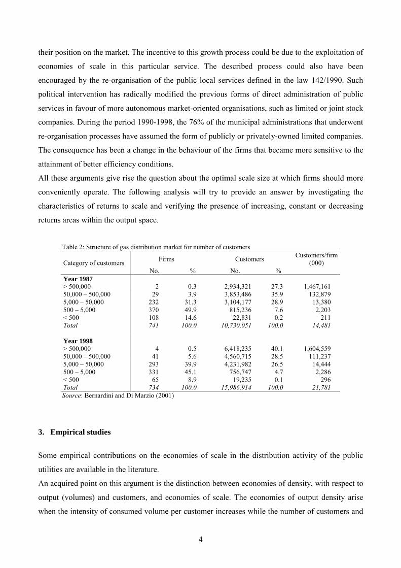
Table 2 presents further evidence confirming the concentration process. During the decade 1987-
1998 the number of small firms (with customers comprised between 500 and 5,000 or less then 500)
reduced, even if they continued to prevail in the distribution market. The percentages indicate a fall
of around 5% in both the categories. On the other hand, the largest units have experienced a growth
of their relative incidence, especially for the category of firms with customers ranging between
5,000 and 500,000 (from 31.3% to 39.9%).
Turning to the number of customers, it is possible to observe that its absolute amount declines for
the lower categories while increases for the upper ones, although the relative shares show a
generalised reduction, except for the main national operators.
In summary, the available evidence supports the thesis that the local distributors have undertaken an
enlargement of their scale size even in the form of mergers and acquisitions, in order to consolidate
4
their position on the market. The incentive to this growth process could be due to the exploitation of
economies of scale in this particular service. The described process could also have been
encouraged by the re-organisation of the public local services defined in the law 142/1990. Such
political intervention has radically modified the previous forms of direct administration of public
services in favour of more autonomous market-oriented organisations, such as limited or joint stock
companies. During the period 1990-1998, the 76% of the municipal administrations that underwent
re-organisation processes have assumed the form of publicly or privately-owned limited companies.
The consequence has been a change in the behaviour of the firms that became more sensitive to the
attainment of better efficiency conditions.
All these arguments give rise the question about the optimal scale size at which firms should more
conveniently operate. The following analysis will try to provide an answer by investigating the
characteristics of returns to scale and verifying the presence of increasing, constant or decreasing
returns areas within the output space.
Table 2: Structure of gas distribution market for number of customers
Firms Customers Customers/firm(000)Category of customers
No. % No. %Year 1987> 500,000 2 0.3 2,934,321 27.3 1,467,16150,000 – 500,000 29 3.9 3,853,486 35.9 132,8795,000 – 50,000 232 31.3 3,104,177 28.9 13,380500 – 5,000 370 49.9 815,236 7.6 2,203< 500 108 14.6 22,831 0.2 211Total 741 100.0 10,730,051 100.0 14,481
Year 1998> 500,000 4 0.5 6,418,235 40.1 1,604,55950,000 – 500,000 41 5.6 4,560,715 28.5 111,2375,000 – 50,000 293 39.9 4,231,982 26.5 14,444500 – 5,000 331 45.1 756,747 4.7 2,286< 500 65 8.9 19,235 0.1 296Total 734 100.0 15,986,914 100.0 21,781Source: Bernardini and Di Marzio (2001)
3. Empirical studies
Some empirical contributions on the economies of scale in the distribution activity of the public
utilities are available in the literature.
An acquired point on this argument is the distinction between economies of density, with respect to
output (volumes) and customers, and economies of scale. The economies of output density arise
when the intensity of consumed volume per customer increases while the number of customers and

5
the size of network system remains unchanged. The economies of customer density arise when
volumes and number of customers increase proportionally holding unchanged the size of the
network.
Economies of scale relate to the case in which volumes, customers and network increase at the same
proportion.
Elasticity of scale directly affects the firm’s maximal profit (Førsund and Hjalmarrson, 2002b).
Moreover returns to scale are an important element to consider in valuating eventual merging
between two or more adjacent distributors. In general, however, the characterisation of returns to
scale in the gas distribution industry still remains unclear.
The characterisation of the technology in the energy sectors (gas and electricity) were largely
investigated in the literature.
The technology underlying the gas distribution is analysed by Guldmann (1983, 1984, 1985); Kim
and Lee (1996); Lee et al. (1999); Fabbri et al. (2000); Hollas et al. (2002). Guldman (1983)
proposed the estimation of a neo-classical cost function to model the structure of the urban gas
distribution. The empirical results allowed to assume the presence of weak economies of scale. The
remaining Guldmann’s contributions point out that economies of scale are not constant and the
average costs vary with the market size and territorial concentration of the customers.
Kim and Lee used a hedonic cost function to model the distribution technology of the Korean gas
industry over the period 1987-1992. They found that almost all of the firms were located in the
increasing returns to scale region in the early period and gradually exhausted scale economies in the
later period.
Lee et al. compared the total factor productivity growth over time between US, Canada, France,
Italy, Japan and Korea. In their cross-country analysis almost all of the firms result to operate under
increasing returns to scale. Economies of scale appear a fundamental determinant of the average
productivity in those countries with a premature industry. Instead, for the countries characterised by
a mature natural gas industry technological progress is the main contributing factor for productivity
growth.
Fabbri et al. proposed an empirical investigation of the Italian gas distribution industry by means of
a long-term cost function. Their analysis highlights the important role of the morphologic and
demographic variables in explaining costs differences and suggests the hypothesis of prevailing
constant economies of scale.
Hollas et al. examined technical efficiency, economies of scale and efficiency changes for the US
gas distribution utilities during the period 1975-1994 by means of Data Envelopment Analysis. As

6
regards economies of scale the results suggest that promotion of competition has generally moved
gas distributors to excessive scale-down processes corresponding to a reduction in scale efficiency.
The technology underlying the electrical distribution is analysed by Clagget (1994); Kumbhakar
and Hjalmarsson (1998); Bagdadioglu et al.(1996). Clagget’s estimates show that Tennessee Valley
Authority (TVA) distributors present increasing as well decreasing scale economies when physical
volumes, number of customers and size of the service area change proportionally. Kumbhakar and
Hjalmarsson focused on productive efficiency in Swedish retail electricity distribution using
hedonic output(s) constructed from physical outputs and their qualities and network characteristics.
The elasticity of scale is found to vary considerably across firms. Bagdadioglu et al. utilised DEA
methodology to analyse the performance of public and private Turkish electric distributors. They
found evidence of scale economies and firms appear symmetrically scale inefficient in both the
increasing and decreasing returns regions.
4. DEA methodology
Knowledge of the nature of returns to scale is realised by applying DEA methodology (Charnes et
al., 1978). It consists in the identification of a non-parametric piecewise linear frontier representing
the best practice in the transformation of a bundle of inputs into final outputs (the theoretical
description of DEA is drawn heavily from Cooper et al., 2000 and Thanassoulis, 2001).
A transformation process can be based on the hypothesis of constant returns to scale (CRS),
although in most general real life contexts it should be more appropriately assumed a variable
returns to scale (VRS) technology. This occurs because the operational size under which a DMU
operates can affect the average productivity. The main consequence is that a DMU should be better
compared with similar DMUs in term of scale of production, especially when a large heterogeneity
in size occurs. Alternatively, a small DMU, for instance, could result inefficient if compared to a
larger one uniquely because of its scale property rather than pure intrinsic inefficiency. In such a
way, the risk of putting forward erroneous judgements on efficiency determinants arises.
When using DEA an alternative occurs in the identification of inefficiency. It is possible to
minimise the use of inputs given the outputs or to maximise the outputs given the inputs. As regard
utility services, such as gas distribution, the output is linked to the local demand while the costs
saving appears to be a more rationale managerial objective. For such reasons, the paper will analyse
the efficiency conditions using an input-oriented projection model.
Given N DMUs (j=1,…N) producing S outputs (r=1,…,S) using M inputs (i=1,…,M), the efficiency
DEA score for a DMU j0 under VRS and input-oriented hypotheses can be estimated by solving the
following linear programme in envelopment form:

7
free.
VRSjj
N
1jj
ij
N
1jjij
VRSj
N
1jrjrjj
VRSj
0
00
0
0
,,...,N1 j0λ
1λ
,...,M1 i0xλx
,...,S1 r 0yyλ
s.t.
Min
θ=≥
=
=≥−θ
=≥−
θ
∑
∑
∑
=
=
=
[1]
Here the non-negative λ-weights measure the contribution of selected Pareto-efficient DMUs to the
definition of a reference point for the inefficient unit j0. The convexity constraint ∑ ==N
j j11λ imposes
of assessing the efficiency under VRS. The optimal solution of [1], VRSj0
θ̂ , is non negative and less
than 1, being equal to unity when full efficiency in the use of inputs occurs. The measure (1- VRSj0θ̂ )
represents the potential radial reduction in inputs, given the output, until the inefficient point is
projected on a surface of the linear piecewise frontier.
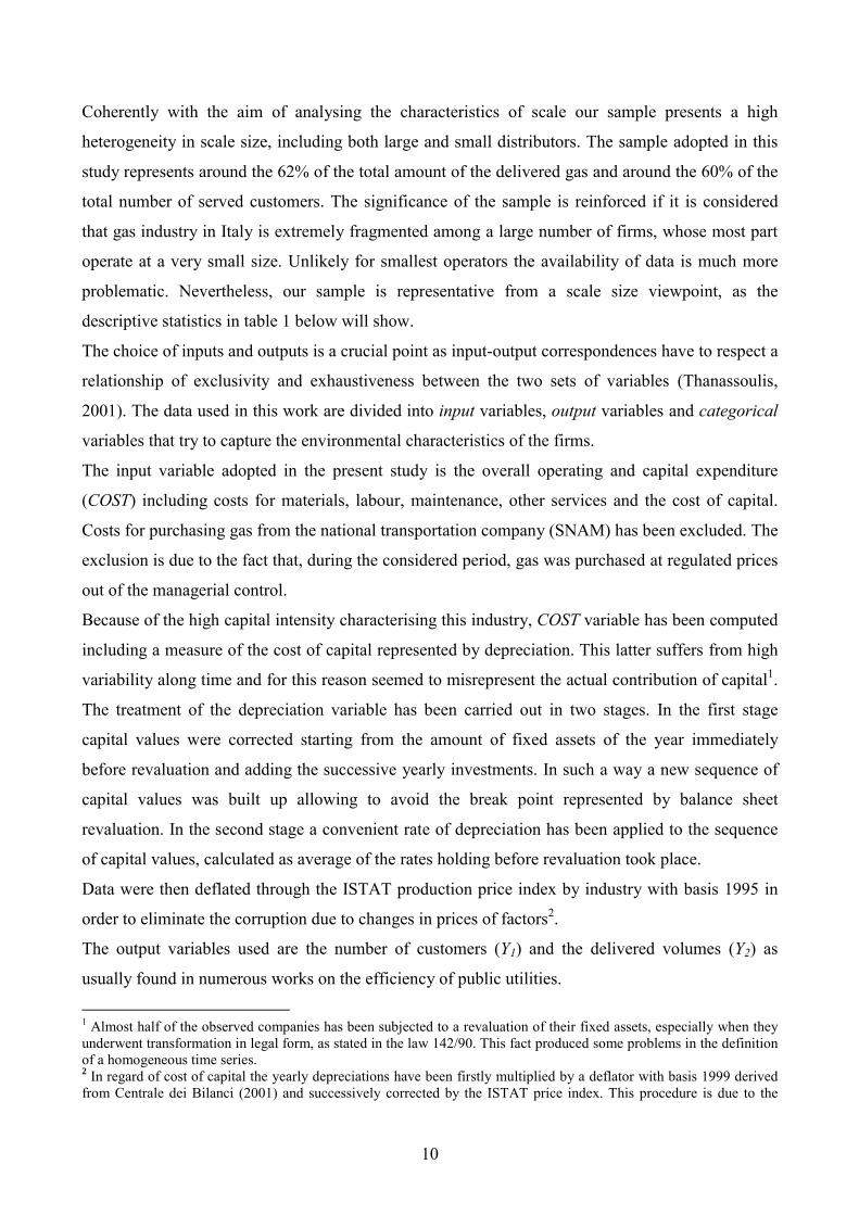
In figure 1 the input-oriented frontier, in a simplified single-output single-input model, is
constructed using both CRS and VRS technology. The areas to the right of the two frontiers
represent the production possibility sets (PPS) under both the assumption of returns to scale. They
are composed by all the points feasible in principle, given the production technology, but affected
by inefficiency.
Figure 1: CRS and VRS frontiers
Points a and d are inefficient and their input-oriented path of projection individualizes referent
points a’ and d’ on VRS frontier and a” and d” on CRS frontier. The unique difference between a”
and a’ or d” and d’ is due to control for scale. The ratios Aa”/Aa’ and Dd”/Dd’ represent the
measure of scale efficiency ( SEaθ̂ and SE
dθ̂ ), while the ratios Aa’/Aa and Dd’/Dd identify the pure
CRS
VRS
a
d
P3
P2
P1
a” a'
d'd”
y
x
A
D
8
technical input efficiency ( VRSaθ̂ and VRS
dθ̂ ) which is exclusively attributable to managerial effort.
The shape of the VRS piecewise boundary is closer to the observed inefficient points so that
efficiency scores under VRS result higher than corresponding CRS measures. The rationale for this
is that CRS measures incorporate a scale inefficiency while VRS measures do not.
The difference occurring between points a and d is that they are characterised by opposite scale
properties. Point a is radially projected on an increasing returns to scale facet of the VRS frontier
while point d is radially projected on a VRS surface where locally decreasing returns to scale hold.
Numerous studies in DEA literature attend to the identification of scale economies (Färe et al.,
1983; Banker et al., 1984; Banker, 1984; Banker and Thrall, 1992; Coelli et al., 1998; Kerstens and
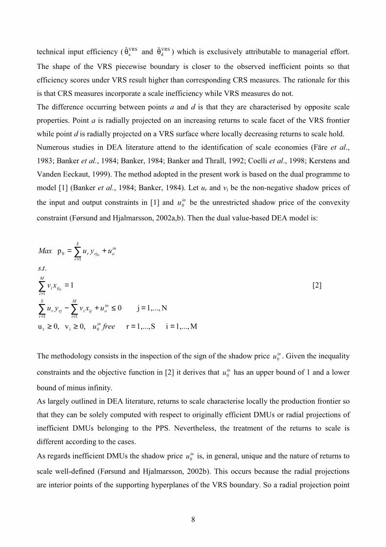
Vanden Eeckaut, 1999). The method adopted in the present work is based on the dual programme to
model [1] (Banker et al., 1984; Banker, 1984). Let ur and vi be the non-negative shadow prices of
the input and output constraints in [1] and inu0 be the unrestricted shadow price of the convexity
constraint (Førsund and Hjalmarsson, 2002a,b). Then the dual value-based DEA model is:
M1,...,i S1,...,r ,0 v,0u
N1,...,j 0
1
..
p
0ir
11
1
10
0
0
==≥≥
=≤+−
=
+=
∑∑
∑
∑
==
=
=
freeu
uxvyu
xv
ts
uyuMax
in
ino
M
iiji
S
rrjr
M
iiji
ino
S
rrjr
[2]
The methodology consists in the inspection of the sign of the shadow price inu0 . Given the inequality
constraints and the objective function in [2] it derives that inu0 has an upper bound of 1 and a lower
bound of minus infinity.
As largely outlined in DEA literature, returns to scale characterise locally the production frontier so
that they can be solely computed with respect to originally efficient DMUs or radial projections of
inefficient DMUs belonging to the PPS. Nevertheless, the treatment of the returns to scale is
different according to the cases.
As regards inefficient DMUs the shadow price inu0 is, in general, unique and the nature of returns to
scale well-defined (Førsund and Hjalmarsson, 2002b). This occurs because the radial projections
are interior points of the supporting hyperplanes of the VRS boundary. So a radial projection point

9
exhibits increasing returns to scale if inu0 > 0, decreasing returns to scale if inu0 < 0 and constant
returns to scale if inu0 = 0.
As regards Pareto-efficient DMUs a problem of multiple optimal solutions arises. This fact can be
better appreciated turning to the previous figure 1. The efficient point P2, for instance, lies on the
edge point that separates two linear facets characterised by different scale regimes. The multiplicity
of the facets which the originally efficient DMUs belong to generates alternative optimal solutions
for inu0 .
Banker and Thrall (1992) provided a generalisation of this method for dealing with the presence of
multiple optimal solutions, by means of the identification of the maximal and minimal admissible
values of inu0 , allowing the identification of the nature of returns to scale for such DMUs.
Finally, following Førsund and Hjalmarsson (1996), the scale elasticity for the input-oriented
projection point of a generic DMU j0 is estimated as:
( ) ˆ
ˆˆ
0j
j
0
0
000 inVRS
VRS
jVRSjj u
xθ,y−
=θ
θε .
Even in this case, the presence of multiple solutions provides the existence of upper and lower
bounds for ε (Löthgren and Tambour, 1996). In Banker and Thrall (1992) can be, once again, found
the extension of the method aimed to solve the alternative solutions problem. At least for originally
inefficient DMUs, an elasticity parameter equal to 1 indicates that the scale is technically optimal,
that is the average productivity is maximal. Values greater than 1 indicate that the radial projection
is on a facet of the VRS boundary where locally increasing returns to scale hold, while values
comprised between 0 and 1 correspond to decreasing returns to scale.
5. Description of the sample
5.1 Input and output variables
Data are available on a sample of 46 gas distributors observed over the period 1994-1999, that is
before the introduction of the liberalisation act, yielding a whole sample of 276 individual
observations. The data have been taken from the database managed by CERIS that collects the
balance sheets of firms providing public services and includes both economic and technical
information. The Italian gas distribution system has not been subjected in these years to radical
regulatory reforms so as to justify the pooling treatment of the panel. The yearly productivity
growth on the same period has been quite low (+0.22%), as found in Fraquelli and Erbetta (2003).
10
Coherently with the aim of analysing the characteristics of scale our sample presents a high
heterogeneity in scale size, including both large and small distributors. The sample adopted in this
study represents around the 62% of the total amount of the delivered gas and around the 60% of the
total number of served customers. The significance of the sample is reinforced if it is considered
that gas industry in Italy is extremely fragmented among a large number of firms, whose most part
operate at a very small size. Unlikely for smallest operators the availability of data is much more
problematic. Nevertheless, our sample is representative from a scale size viewpoint, as the
descriptive statistics in table 1 below will show.
The choice of inputs and outputs is a crucial point as input-output correspondences have to respect a
relationship of exclusivity and exhaustiveness between the two sets of variables (Thanassoulis,
2001). The data used in this work are divided into input variables, output variables and categorical
variables that try to capture the environmental characteristics of the firms.
The input variable adopted in the present study is the overall operating and capital expenditure
(COST) including costs for materials, labour, maintenance, other services and the cost of capital.
Costs for purchasing gas from the national transportation company (SNAM) has been excluded. The
exclusion is due to the fact that, during the considered period, gas was purchased at regulated prices
out of the managerial control.
Because of the high capital intensity characterising this industry, COST variable has been computed
including a measure of the cost of capital represented by depreciation. This latter suffers from high
variability along time and for this reason seemed to misrepresent the actual contribution of capital1.
The treatment of the depreciation variable has been carried out in two stages. In the first stage
capital values were corrected starting from the amount of fixed assets of the year immediately
before revaluation and adding the successive yearly investments. In such a way a new sequence of
capital values was built up allowing to avoid the break point represented by balance sheet
revaluation. In the second stage a convenient rate of depreciation has been applied to the sequence
of capital values, calculated as average of the rates holding before revaluation took place.
Data were then deflated through the ISTAT production price index by industry with basis 1995 in
order to eliminate the corruption due to changes in prices of factors2.
The output variables used are the number of customers (Y1) and the delivered volumes (Y2) as
usually found in numerous works on the efficiency of public utilities.
1 Almost half of the observed companies has been subjected to a revaluation of their fixed assets, especially when theyunderwent transformation in legal form, as stated in the law 142/90. This fact produced some problems in the definitionof a homogeneous time series.2 In regard of cost of capital the yearly depreciations have been firstly multiplied by a deflator with basis 1999 derivedfrom Centrale dei Bilanci (2001) and successively corrected by the ISTAT price index. This procedure is due to the
11
Finally, the length of network (LN) has been included in our study as categorical variable, in order
to capture the different behaviour of firms operating under particular degree of customers
concentration, as in the cases of urban and rural areas.
5.2 Descriptive statistics
Table 3 summarises some descriptive statistics relative to the sample. The main evidence is that
DMUs are spanned over a very wide output space, that includes a high variety in scale size, as
shown by the coefficients of variation, calculated as ratio between standard deviation and mean
values. The results show a standard deviation being three times the average value of each variable.
All the outputs appear positively correlated with COST variable. The corresponding index is in all
cases approximately equal to 1 so indicating a high explanatory power of the dynamic of operating
and capital expenditures. The high variety that characterises the length of network confirms the
heterogeneity of the environment contexts at which the firms operate, reflecting the state of the
Italian gas distribution system.
Notice finally that the distance between the third quartile and the maximal value is due to the
presence in our sample of ITALGAS, that is the main national public-owned distributor.
Table 3: descriptive statistics
Min 1st quartile 3rd quartile max mean var. coeff. Correlationindex
Y1 (no. customers) 2,708 18,344 111,357 4,458,000 19,3348 3.15 0.996Y2 (mil. of cubic meters) 6.0 41.5 193.8 7,100.0 301.3 3.12 0.991Y3 (km of network) 39.4 253.3 1,064.8 3,6271.0 1,661.2 2.97 0.983
5.3 Economies of scale and density
The economic efficiency is theoretically decomposed in scale efficiency and technical efficiency.
Scale efficiency is related to the economies that arise when all outputs (volumes and customers) and
network increase proportionally. Technical efficiency under VRS assumption, instead, indicates the
internal managerial ability to maximise the economic performance leaving out of consideration the
operational scale. Technical efficiency can be affected by economies of density with respect to
output and customers.
nature of capital variable, characterised by a stratification over time of the investments. In such a way is has beenpossible to express the depreciation in an homogeneous monetary power.

12
Figure 2 shows the dynamic of the average cost corresponding to an increase of customers per
kilometre of network (a) and of volumes per customer (b). The average cost with respect to
customers confirm the presence of economies of customer density while the average cost with
respect to delivered volumes confirm the presence of economies of output density. For what it
concerns figure 2a the median of the ratio costumers/network is around 100 and this value has been
used for discriminating between DMUs characterised by high and low customer density.
Figure 2: Economies of output and customer density
Anyway both output and customer density are environmental characteristics out of managerial
control that necessitate of specific treatments.
As regards economies of output density, the simultaneous presence of Y1 and Y2 allows to treat these
economies as endogenous. In fact, given the output Y2, the efficiency of those DMUs with a high
number of customers, and then with low output density, increases while the efficiency of those
DMUs with a low number of customers, and then a high degree of output density, decreases3.
With regards economies of customer density two possible solutions can be proposed.
The first one is more practical and suggests the consideration of the variable LN as output so as to
DMUs with high network extension and then low customer density are allowed to increase their
score efficiency, while the opposite would occur for DMUs that take advantage from higher density
effect.
The second one, instead, is based on the use of a density measure, calculated as ratio between
customers and length of network, as categorical variable (Banker and Morey, 1986; Charnes et al.,
1994; Thanassoulis, 2001). This control for density lies upon the a priori assumption that higher the
number of customers for each kilometre of network higher the productivity advantage would be.
3 In order to isolate the output density effect it would be necessary to run a DEA model based on one output (volumes)and one input. A similar model, however, seems not admissible in practice, because of the consequent lack ofdiscrimination among firms, and in theory, given the well established use in the literature of two output models.
100 200 300 400 500 600 700 800
0 50 100 150 200 250 300 Customers/network
(a)
COST
(000
)/cus
tom
ers
0 100 200 300 400 500 600 700
0 0,001 0,002 0,003 0,004 0,005 Volumes/customers
(b)
COST
/vol
umes
13
The main insight is that DMUs that enjoy a higher advantage in term of average productivity by
virtue of density effects, could not be taken as referent points for DMUs that are less advantaged,
while the inverse is admissible (Thanassoulis, 2001).
This latter solution seemed more appropriate and has been adopted in this study because of its
stronger theoretical background an also because it seemed more correct to use LN as categorical
variable rather than as output itself. In order to implementing this procedure, the sample has been
split into two subsets of DMUs (Sd, with d = 1 and 2), the first one corresponding to the less
advantaged and the second one corresponding to the more advantaged units. The comparison
between more advantaged and less advantaged DMUs by virtue of potential density effect has been
limited by modifying the constraints of [2], so that the linear programming for a generic DMU j0
belonging to subset d becomes:
M1,...,i S1,...,r ,0 v,0u
Sj 0
1
..
p
0ir
d
1kk
11
1
10
0
0
==≥≥
∈≤+−
=
+=
===
=
=
∑∑
∑
∑
freeu
uxvyu
xv
ts
uyuMax
in
ino
M
iiji
S
rrjr
M
iiji
ino
S
rrjr
!
[3]
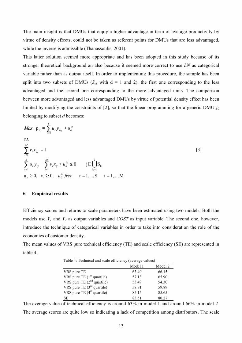
6 Empirical results
Efficiency scores and returns to scale parameters have been estimated using two models. Both the
models use Y1 and Y2 as output variables and COST as input variable. The second one, however,
introduce the technique of categorical variables in order to take into consideration the role of the
economies of customer density.
The mean values of VRS pure technical efficiency (TE) and scale efficiency (SE) are represented in
table 4.Table 4: Technical and scale efficiency (average values) Model 1 Model 2VRS pure TE 63.40 66.15VRS pure TE (1st quartile) 57.13 65.90VRS pure TE (2nd quartile) 53.49 54.30VRS pure TE (3rd quartile) 58.91 59.89VRS pure TE (4th quartile) 85.15 85.65SE 83.51 80.27
The average value of technical efficiency is around 63% in model 1 and around 66% in model 2.
The average scores are quite low so indicating a lack of competition among distributors. The scale
14
component is, instead, characterised by an efficiency level of 80-83%. Due to the high variability in
scale size, the observations has been grouped into quartiles, calculated on the basis of the number of
customers. In both the models the first 75% of the DMUs lies below 60% of pure technical
efficiency while the latter 25% presents values of 80-83%. This latter result, however, should be
treated with caution because the group of greatest units could benefit of high technical efficiency
uniquely because of a lack of comparison with other DMUs. In fact, when few firms operate spot at
very high scale size, in absence of an adequate comparison with other DMUs they assume a high
score efficiency as DEA uses them as best practice points.
The passage from model 1 to model 2 points out an average increase in pure technical efficiency of
3%, which is particularly significant for the first quartile (9%). This gives rise questions on the role
played by the effect of customer density. The firms serving few customers are likely to operate
under low density of network that bestows a productivity disadvantage with respect to firms
operating under higher density conditions. The increasing in efficiency observed for model 2
reveals the penalisation in which low density firms have been incurred when compared with high
density firms.
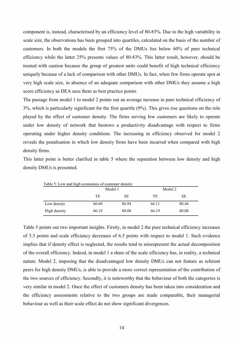
This latter point is better clarified in table 5 where the separation between low density and high
density DMUs is presented.
Table 5: Low and high economies of customer densityModel 1 Model 2
TE SE TE SE
Low density 60.60 86.94 66.11 80.46
High density 66.19 80.08 66.19 80.08
Table 5 points out two important insights. Firstly, in model 2 the pure technical efficiency increases
of 5.5 points and scale efficiency decreases of 6.5 points with respect to model 1. Such evidence
implies that if density effect is neglected, the results tend to misrepresent the actual decomposition
of the overall efficiency. Indeed, in model 1 a share of the scale efficiency has, in reality, a technical
nature. Model 2, imposing that the disadvantaged low density DMUs can not feature as referent
peers for high density DMUs, is able to provide a more correct representation of the contribution of
the two sources of efficiency. Secondly, it is noteworthy that the behaviour of both the categories is
very similar in model 2. Once the effect of customers density has been taken into consideration and
the efficiency assessments relative to the two groups are made comparable, their managerial
behaviour as well as their scale effect do not show significant divergences.

15
The evaluation of the scale efficiency allows to identify the output space areas where decreasing or
increasing returns hold as well the optimal scale at which a gas distributor should operate in order to
maximise its average productivity (MPSS, Most Productive Scale Size).
In figure 3 scale efficiency has been plotted against a scale variable identified by the number of
served customers. The shape of the curve is regular, showing increasing returns before
approximately 65,000 customers and decreasing returns after this threshold4. The optimal scale is
univocally determined and corresponds to 65,000 customers in both the models. Notice moreover
that almost the half of the observations show a scale efficiency greater than 90%.
The same analysis conducted with respect to delivered volumes provided an optimal scale
corresponding to approximately 150 millions of cubic meters .
Figure 3: identification of optimal scale , DRS and IRS areas
The regulatory act (Decree 164/2000), establishing some circumstances that permit to benefit of the
delay of the public tender for the franchise assignment, indicates respectively a higher threshold as
regards customers (100,000 units) and a lower threshold as regards volumes (100 millions of yearly
cubic meters) with respect to the optimal scale found out in our study.
The analysis of elasticity of scale can contribute to the comprehension of the scale properties.
Elasticity of scale (εjo) measures the relative marginal increases in all outputs corresponding to a
relative marginal increase in input. A value of elasticity greater than 1 indicates increasing returns
to scale. A value of elasticity lesser than 1 indicates decreasing returns to scale. Finally a value of
elasticity equal to 1 indicates that the DMU operate at optimal scale.
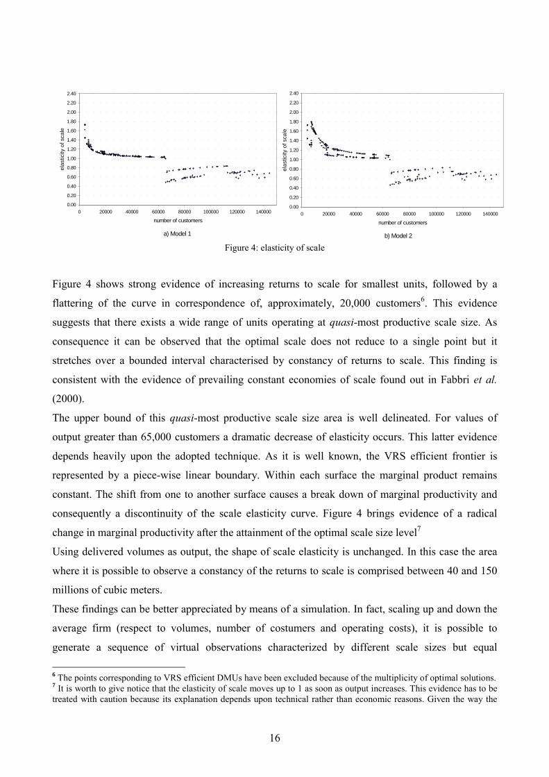
In figure 4 the values of elasticity have been plotted against the number of customers5.
4 The horizontal axis has been truncated at 1,000,000 customers but the curve maintains its regularity even for greaterscale sizes.5 The horizontal axis has been truncated at 150,000 customers but the curve maintains its regularity even for greaterscale sizes.
a) Model 1
40.00
50.00
60.00
70.00
80.00
90.00
100.00
0 100000 200000 300000 400000 500000 600000 700000 800000 900000 1000000
number of customers
scal
e ef
ficie
ncy
b) Model 2
30.00
40.00
50.00
60.00
70.00
80.00
90.00
100.00
0 100000 200000 300000 400000 500000 600000 700000 800000 900000 1000000
number of customers
scal
e ef
ficie
ncy
16
Figure 4: elasticity of scale
Figure 4 shows strong evidence of increasing returns to scale for smallest units, followed by a
flattering of the curve in correspondence of, approximately, 20,000 customers6. This evidence
suggests that there exists a wide range of units operating at quasi-most productive scale size. As
consequence it can be observed that the optimal scale does not reduce to a single point but it
stretches over a bounded interval characterised by constancy of returns to scale. This finding is
consistent with the evidence of prevailing constant economies of scale found out in Fabbri et al.
(2000).
The upper bound of this quasi-most productive scale size area is well delineated. For values of
output greater than 65,000 customers a dramatic decrease of elasticity occurs. This latter evidence
depends heavily upon the adopted technique. As it is well known, the VRS efficient frontier is
represented by a piece-wise linear boundary. Within each surface the marginal product remains
constant. The shift from one to another surface causes a break down of marginal productivity and
consequently a discontinuity of the scale elasticity curve. Figure 4 brings evidence of a radical
change in marginal productivity after the attainment of the optimal scale size level7
Using delivered volumes as output, the shape of scale elasticity is unchanged. In this case the area
where it is possible to observe a constancy of the returns to scale is comprised between 40 and 150
millions of cubic meters.
These findings can be better appreciated by means of a simulation. In fact, scaling up and down the
average firm (respect to volumes, number of costumers and operating costs), it is possible to
generate a sequence of virtual observations characterized by different scale sizes but equal
6 The points corresponding to VRS efficient DMUs have been excluded because of the multiplicity of optimal solutions.7 It is worth to give notice that the elasticity of scale moves up to 1 as soon as output increases. This evidence has to betreated with caution because its explanation depends upon technical rather than economic reasons. Given the way the
a) Model 1
0.00
0.20
0.40
0.60
0.80
1.00
1.20
1.40
1.60
1.80
2.00
2.20
2.40
0 20000 40000 60000 80000 100000 120000 140000
number of customers
elas
ticity
of s
cale
b) Model 2
0.00
0.20
0.40
0.60
0.80
1.00
1.20
1.40
1.60
1.80
2.00
2.20
2.40
0 20000 40000 60000 80000 100000 120000 140000
number of customers
elas
ticity
of s
cale

17
operational attributes. DEA has been running starting from a panel composed by real and virtual
observations. These latter are inefficient by construction so that to do not modify previous DEA
frontier.
Table 6 presents the estimates of the elasticity of scale. For the smallest firms (below 10% of the
average firm) the returns to scale are very strong and exhaust rapidly. Successively it is possible to
observe a more gradual decreasing in the elasticity parameter. Notice, finally, the strong break
down of the elasticity between 30% and 40% of the average firm, that is when the optimal scale size
is overran.
Table 6: Elasticity of scale
ObservationsVolumes
(mil. of cubic meters)Number of customers Elasticity of scale
3% average firm 9.0 5,801 1.320
5% average firm 15.1 9,667 1.192
10% average firm 30.1 19,335 1.096
20% average firm 60.3 38,670 1.048
30% average firm 90.4 58,005 1.032
40% average firm 120.5 77,339 0.764
average firm 301.3 193,348 0,746
7 Conclusions and policy remarks
The Italian gas distribution industry presents a high degree of fragmentation. More than 700
operators provide the service to final customers. They operate at very different scale sizes and this
fact could arise questions about the most convenient dimension. The regulatory act 164/2000
indirectly provides an indication of 100,000 customers and 100 millions of cubic meters as output
values compatible with a regime of optimal scale size.
The purpose of this study has been to estimate the characteristics of technical and scale efficiency of
the Italian gas distributors. DEA methodology has been adopted in order to construct an efficient
boundary against which to measure the degree of efficiency of the involved units.
The results of our study can be summarised as follows.
1) The level of the technical efficiency is equal, on average, to 63-66%. This means that the same
levels of output could be provided using the 63-66% of the original amount of input. This score
VRS boundary is built up, as soon as output increases the average product converges towards marginal product soyielding the return to 1 of the elasticity curve.

18
of efficiency seems very low so indicating a lack of competition within the distribution system.
Therefore the evidence suggests a strong need of regulatory rules that can replicate competitive
conditions. The scale efficiency is higher and equal to, on average, 80-83%.
2) The inclusion in the model of the effect of customer density permits to evaluate the degree of
penalisation suffered by low density DMUs. When low density DMUs are directly compared
with high density DMUs DEA tends to underestimate technical efficiency and overestimate
scale efficiency to a significant extent, so providing a wrong decomposition of the overall
efficiency.
3) Optimal scale is attained at around 65,000 customers and 150 millions of cubic meters. These
results do not fully match the indication putted forward by the regulator. However, it is
interesting to note that a wide range in output space there exists where quasi-most productive
scale size is attained. Increasing returns to scale become rapidly exhausted and after around
20,000 customers and 40 millions of cubic meters the curve of scale elasticity flats on unitary
value.
From a regulatory viewpoint our main conclusion is that the search of better productivity conditions
could be based on merging processes that involve the smallest units serving less than 20,000
customers or delivering less than 40 millions of cubic meters, that is the lower bounds of the area
where quasi-constant returns to scale hold. Given the extreme fragmentation of the service on the
Italian territory, this merging process could contribute to substantially reduce the existing number of
distributors. Governmental interventions should encourage the concentration process that has
already took place during the 90s. Indeed, the recent liberalisation of the gas industry seems
addressed to grant a strategic valence to the scale set up.
Finally, since the critical size required to exploit economies of scale is not so large and substantially
inferior to the optimal dimension, the concentration process in the distribution gas industry can be
viewed as a very “attainable” objective.

19
References
Bagdadioglu N., Waddam Price C.M., Weyman-Jones T.G., 1996, “Efficiency and ownership in
electricity distribution: A non-parametric model of the Turkish experience”, Energy Economics,
no.18, pp 1-23.
Banker R.D., 1984, “Estimating most productive scale size using data envelopment analysis”
European Journal of Operational Research, no.17, pp 35-44.
Banker R.D., Morey R.C., 1986, “The use of categorical variables in Data Envelopment Analysis”,
Management Science, no. 32(12), pp1613-1627.
Banker R.D., Thrall R.M., 1992, “Estimation of returns to scale using Data Envelopment Analysis”,
European Journal of Operational Research, no. 62, pp 74-84.
Banker R.D.,Charnes A., Cooper W.W., 1984, “Some models for estimating technical and scale
inefficiencies in Data Envelopment Analysis”, Management Science, no. 30, pp 1078-1092.
Bernardini O., Di Marzio T., 2001, “La distribuzione del gas a mezzo reti urbane in Italia: analisi
del settore alla vigilia della liberalizzazione”, Autorità per l’energia elettrica e il gas.
Charnes A., Cooper W. W., Lewin Y.A., Seiford M.L.,1994, Data Envelopment Analysis: Theory,
Methodology and Applications, Kluwer Academic Publishers, Boston/Dordrecht/London.
Charnes A., Cooper W.W., Rhodes E., 1978, “Measuring the efficiency of decision making units”,
European Journal of Operational Research, no. 2, pp 429-444.
Claggett E.T., 1994, “A cost function study of the providers of TVA power”, Managerial and
Decision Economics, no. 15, pp 63-72.
Coelli T., Prasada Rao D.S., Battese G.E., 1998, An introduction to efficiency and productivity
analysis, Kluwer Academic Publishers, Boston/Dordrecht/London.
Cooper W.W., Seiford L.M., Tone K., 2000, Data Envelopment Analysis, Kluwer Academic
Publishers, Boston/Dordrecht/London.
Fabbri P., Fraquelli G., Giandrone R., 2000, “Costs, technology and ownership of gas distribution
in Italy”, Managerial and Decision Economics, no. 21, pp 71-81.
Färe R.,Grosskopf S., Lovell C.A.K., 1983, “The structure of technical efficiency”, Scandinavian
Journal of Economics, no. 85, pp 181-90.
Førsund F.R., Hjalmarsson L., 1996, “Measuring returns to scale of piecewise linear multiple output
technologies: Theory and empirical evidence”, Memorandum n.223, Department of Economics,
School of Economics and Commercial Law, Göteborg University.
Førsund F.R., Hjalmarsson L., 2002a, “Are all scales optimal in DEA? Theory and empirical
evidence”, Working Paper Series, n.14, ICER, Turin.
20
Førsund F.R., Hjalmarsson L., 2002b, “Calculating the scale elasticity in DEA models”, Working
Paper Series n.28, ICER, Turin.
Fraquelli G., Erbetta F., 2003, “Aspetti gestionali e analisi dell’efficienza nel settore della
distribuzione di gas”, L’Industria, n.4.
Guldmann J.M., 1983, “Modelling the structure of gas distribution costs in urban areas”, Regional
Science and Urban Economics, no. 13, pp 299-316.
Guldmann J.M., 1984, “A further note on the structure of gas distribution costs in urban areas”,
Regional Science and Urban Economics, no. 14, pp 583-588.
Guldmann J.M., 1985, “Economies of scale and natural monopoly in urban utilities: the case of
natural gas distribution”, Geographical Analysis, no. 17, pp 302-317.
Hollas D.R., Macleod K.R., Stansell S.R., 2002, “A Data Envelopment Analysis of gas
utilities’efficiency”, Journal of Economics and Finance, no. 26, pp 123-137.
Kerstens K., Vanden Eeckaut P., 1999, “Estimating returns to scale using non-parametric
deterministic technologies: A new method based on goodness-of-fit”, European Journal of
Operational Research, no. 113, pp 206-214.
Kim T.Y., Lee J.D., 1996, “Cost analysis of gas distribution industry with spatial variables”, The
Journal of Energy and Development, no. 20, pp 247-267.
Kumbhakar S.C., Hjalmarsson L., 1998, “Relative performance of public and private ownership
under yardstick competition: electricity retail distribution”, European Economic Review, no. 42,
pp 97-122.
Lee J.D., Kyung J.O., Kim T.Y, 1999, “Productivity growth, capacity utilization and technological
progress in the natural gas industry”, Utilities Policy, no. 8, pp109-119.
Lothgren M., Tambour M., 1996, “Alternative approaches to estimate returns to scale in DEA-
models”, Working paper Series in Economics and Finance n.90, Stockolm School of Economics.
Thanassoulis E., 2001, “Introduction to the theory and application of Data Envelopment Analysis”,
Kluwer Academic Publishers, Boston/Dordrecht/London.