Estimating jaguar densities with camera traps:...

Estimating jaguar densities with camera traps: Problems with currentdesigns and recommendations for future studies

Mathias W. Tobler a,⇑, George V.N. Powell b

a San Diego Zoo Global, Institute for Conservation Research, 15600 San Pasqual Valley Road, Escondido, CA 92027-7000, USAb World Wildlife Fund Conservation Science Program, 1250 24th Street, NW, Washington, DC 20037, USA

a r t i c l e i n f o

Article history:Received 28 June 2012Received in revised form 7 December 2012Accepted 8 December 2012

Keywords:Spatially explicit capture recapture model(SECR)Panthera oncaDensity estimationMean maximum distance moved (MMDM)SimulationCamera traps

a b s t r a c t

Camera traps have become the main method for estimating jaguar (Panthera onca) densities. Over 74studies have been carried out throughout the species range following standard design recommendations.We reviewed the study designs used by these studies and the results obtained. Using simulated data weevaluated the performance of different statistical methods for estimating density from camera trap dataincluding the closed-population capture–recapture models Mo and Mh with a buffer of ½ and the fullmean maximum distance moved (MMDM) and spatially explicit capture–recapture (SECR) models underdifferent study designs and scenarios. We found that for the studies reviewed density estimates werenegatively correlated with camera polygon size and MMDM estimates were positively correlated. Thesimulations showed that for camera polygons that were smaller than approximately one home rangedensity estimates for all methods had a positive bias. For large polygons the Mh MMDM and SECR modelproduced the most accurate results and elongated polygons can improve estimates with the SECR model.When encounter rates and home range sizes varied by sex, estimates had a negative bias for models thatdid not include sex as a covariate. Based on the simulations we concluded that the majority of jaguarcamera trap studies did not meet the requirements necessary to produce unbiased density estimatesand likely overestimated true densities. We make clear recommendations for future study designs withrespect to camera layout, number of cameras, study length, and camera placement. Our findings directlyapply to camera trap studies of other large carnivores.

� 2012 Elsevier Ltd. All rights reserved.

1. Introduction

It has been over 16 years since camera traps (infrared activatedcameras) and capture–recapture models were first used to esti-mate the density of a large cat (Karanth, 1995). Many studies haveadopted the methodology and design developed by Karanth andNichols (1998) for their species and few changes or improvementshave been made to this method. Besides the tiger (Panthera tigris),the jaguar (Panthera onca) is the species that has been most studiedwith camera traps. Maffei et al. (2011) documented 83 differentsurveys that have been carried out from Arizona to Argentina withthe goal of documenting the presence and estimating density of thejaguar. Many of these surveys have based their design on a manualwith recommendations on field design and data analysis for jaguarsurveys (Silver, 2004).

Jaguar density is usually estimated from camera trap data usingclosed population capture–recapture models and most studies usethe software package CAPTURE (Otis et al., 1978; Rexstad andBurnham, 1991; White et al., 1982) to estimate abundance. In most

cases the jackknife implementation of the Mh model which ac-counts for heterogeneity in the capture probabilities among indi-viduals is chosen over model M0 which assumes captureprobabilities to be equal for all individuals (Burnham and Overton,1979). Other implementations of the Mh model such as estimatingfunctions (Chao et al., 2001) or the maximum likelihood mixturemodels (Dorazio and Royle, 2003; Pledger, 2000), which allow forindividual covariates, have rarely been used in camera trap studies.

There are two main assumptions made by these closed popula-tion capture–recapture models that influence the design of cameratrap studies (1) population closure, and (2) no individual can havezero capture probability. To ensure population closure, most stud-ies use a short survey length (between 30 and 90 days) duringwhich it is assumed the population will experience no birth,deaths, immigration or emigration. Given that capture probabili-ties are generally low for jaguars, survey length is a trade-off be-tween keeping the survey short enough to assume closure andcolleting enough data for a robust abundance estimation (Harmsenet al., 2011). In order to satisfy the second assumption, that noindividual has zero probability of being photographed, the designhas to ensure that at least one camera station is placed withinthe home range of every individual in the study area. In other

0006-3207/$ - see front matter � 2012 Elsevier Ltd. All rights reserved.http://dx.doi.org/10.1016/j.biocon.2012.12.009

⇑ Corresponding author. Tel.: +1 760747 8702.E-mail address: [email protected] (M.W. Tobler).

Biological Conservation 159 (2013) 109–118

Contents lists available at SciVerse ScienceDirect

Biological Conservation

journal homepage: www.elsevier .com/ locate /biocon

http://crossmark.dyndns.org/dialog/?doi=10.1016/j.biocon.2012.12.009&domain=pdf

http://dx.doi.org/10.1016/j.biocon.2012.12.009

mailto:[email protected]


http://www.sciencedirect.com/science/journal/00063207

http://www.elsevier.com/locate/biocon

words, there should be no hole between cameras that could fit anentire home range of an individual. Many studies cite a minimumhome range of 10 km2 for a female jaguar as estimated by Rabino-witz and Nottingham (1986) based on footprint surveys in Belizeand consequently space cameras at about 2–3 km intervals (e.g.Kelly, 2003; Silveira et al., 2010; Silver et al., 2004). However, giventhat the number of cameras available for a study is usually limited,this minimum distance between cameras also determines themaximum area surveyed, something that has typically received lit-tle attention.

In order to convert abundance into density one needs to esti-mate the effective trapping area (ETA). This is generally done byestimating the mean maximum distance moved (MMDM), whichis supposed to be a proxy for home range diameter and is calcu-lated by taking the average of the maximum distance between cap-ture locations for all individuals captured at a minimum of twocamera stations and then calculating the ETA by applying a bufferof width ½ MMDM around the camera polygon (Karanth and Nic-hols, 1998; Wilson and Anderson, 1985). Three potential problemsarise when using this technique for jaguars which typically havelarge home ranges and low capture probabilities: (1) the possiblemaximum distance is limited by the maximum distance betweencameras which is insufficient to represent home range size of jag-uars, (2) with few recaptures the cameras do not capture the actualmaximum distance moved of an individual within the grid, and (3)the maximum distance moved is underestimated for individualswhose home range only partly overlaps the camera grid. Thesesampling errors can lead to an underestimation of the true MMDMand subsequently the ETA which in turn results in an overestima-tion of density. This has been realized when researchers comparedthe MMDM obtained from camera traps to the MMDM from telem-etry data, and lead to the suggestion that the full MMDM might bea more representative buffer than ½ MMDM (Dillon and Kelly,2008; Sharma et al., 2010; Soisalo and Cavalcanti, 2006).

Over recent years new spatially explicit capture–recapture mod-els (SECR) have been developed that use the spatial location of cap-tures to estimate activity centers, distance parameters (r),encounter rates at the activity center (k0), and abundance for allindividuals in a pre-defined area, avoiding the choice of a buffer toestimate the ETA (Efford, 2004; Efford et al., 2009; Royle and Gard-ner, 2011; Royle and Young, 2008). These models further have theadvantage that they can incorporate both individual-level covari-ates such as sex or age class as well as station level covariates suchas road vs trail, camera type or habitat (Sollmann et al., 2011),whereas classical capture–recapture models for closed populationsbased on a maximum likelihood estimator only allowed for individ-ual covariates and the jackknife estimator does not allow for anycovariates. SECR models make some additional assumptions to theclosed population capture–recapture models (1) home ranges arestable over the time of the survey, (2) activity centers are distributedrandomly (as a Poisson process), (3) home ranges are approximatelycircular, and (4) encounter rate (the expected number of encoun-ters/photographs per sampling interval) declines with increasingdistance from the activity center following a predefined detectionfunction. These models can be analyzed both within a maximum-likelihood (Borchers and Efford, 2008; Efford et al., 2009) as wellas a Bayesian framework (Royle and Gardner, 2011; Royle andYoung, 2008). Simulations showed that the SECR models work welland produce unbiased results for adequate sample sizes (N = 200, rsmaller than grid size) but bias increased with low capture probabil-ities and when the home range size was getting closer to the size ofthe study area (Marques et al., 2011; Royle and Young, 2008). Soll-mann et al. (2011) were the first to apply these models to a jaguarcamera trap study and they found that including sex as well as cam-era location (on/off road) as covariates improved estimates over theclassical method using MMDM and models without covariates.

A recent review based on a literature review and the authorsown experience has brought up several potential problems withcamera trap density studies including misidentification of individ-uals, low capture probabilities, small sample sizes, camera failure,and small study area size (Foster and Harmsen, 2012). However, todate there exist no clear recommendations on what minimum sur-vey effort is needed for jaguar surveys in order to produce accuratedensity estimates. Especially the question of the minimum surveyarea needed in relation to home range size has never been well ad-dressed. Maffei and Noss (2008) compared camera trap data totelemetry data from ocelots and concluded that the survey areashould be three to four times the average home range size, butthere is little theoretical justification for that. Given the wide-spread use of camera trap data for estimating jaguar densities, itis important to evaluate the potential bias of current camera trapstudies caused by inadequate study designs and to make clear rec-ommendations for future studies. We implemented an extensiveseries of simulations to quantitatively measure the bias in jaguardensity calculations as a function of camera polygon size andshape, camera numbers, sampling period and jaguar density. Wesimulated spatially explicit capture–recapture data using realisticparameters for jaguars and camera trap survey designs. Based onour simulations we make specific recommendations for futurestudies, taking into account both statistical as well as logisticconsiderations.

2. Materials and methods

2.1. Review of field studies

We compiled a database of published and unpublished jaguardensity surveys recording the number of cameras used, the num-ber of survey days, the camera spacing, the area of the survey poly-gon, the number of individuals captured, the number of recaptures,the estimated MMDM, the estimated abundance, the estimatedtrapping area, and the estimated density. We also reviewed avail-able publications on jaguar home range size.

We used a linear regression to look at the relationship betweenthe estimated MMDM and the survey polygon area using a log-transformation for polygon area. We used a second linear regres-sion to look at the relationship between estimated density andthe survey polygon using a log-transformation for both variables.For the second regression we excluded one outlier with a densityof 18.3 ind. km�2. All analysis were carried out in R 2.14 (R Devel-opment Core Team, 2011).

2.2. Simulations

We simulated datasets to evaluate which factors influencedboth the accuracy and precision of the classic MMDM based esti-mators as well as different SECR models. We chose parameters thatwe consider realistic for jaguar populations and camera trap stud-ies based on our literature review (Table 1). To simulate the datawe used the function sim.capthist() from the secr package (Efford,2011b) in R 2.14 (R Development Core Team, 2011). This functionsimulates spatially explicit capture recapture data based on ran-domly distributed activity centers, circular home ranges, and anencounter rate that declines with distance from the activity centerfollowing a half-normal function (g(d) = k0 � exp(�d2/(2r2); withk0 = base encounter rate at the activity center, r = distance param-eter related to the home range radius and d = distance between theactivity center and the camera). This is the same model that is usedby the SECR model to estimate density. We truncated the distancefunction at 2.45 � r which corresponds approximately to a 95%home range estimate. Not truncating the data would in some cases

110 M.W. Tobler, G.V.N. Powell / Biological Conservation 159 (2013) 109–118

increase the MMDM estimates due to rare captures at very largedistances from the activity center in larger grids. All simulatedcamera grids for our baseline simulation had a square shape andactivity centers were distributed over an area that incorporatedthe camera grid plus a 6 � r wide buffer on each side of the grid.We only considered scenarios with a minimum of five capturedindividuals given that a lower number of captured individuals of-ten resulted in failed estimates. We estimated densities with theM0 and Mh jackknife estimators and a buffer of ½ MMDM andthe full MMDM as well as with a basic SECR model implementedin secr (Efford, 2011b; Efford et al., 2009). For the basic model withno covariates the maximum likelihood and the Bayesian imple-mentation of the SECR model give almost identical results andwe therefore decided to use the maximum likelihood implementa-tion based on the significantly lower computational time requiredfor each simulation run. We ran 110 repetitions for each of the1404 parameter combinations (Table 1), resulting in 154,440 sim-ulation runs. Simulations were run in parallel using the snowfallpackage (Knaus, 2010).

After analyzing the results from our baseline simulations weconducted further simulations to investigate the effect of cameragrid shape, and sex-specific encounter rates and sex-specific homerange sizes on estimates as well as to evaluate the possibility ofcorrecting estimates setting the MMDM or r value to the know va-lue used for the simulations. For these simulations we used a re-duced set of parameters at intermediate levels. We used 60survey days, densities of 2 and 4 ind. 100 km�2, and all the polygonsizes used for the original simulations. For the simulations wherewe set MMDM and r to the simulated value we used a 7 � 7 grid,r values of 2857 m and 4592 m and a k0 of 0.01. Due to truncationthe estimated r is lower than the simulated r so that we used acorrection factor of 0.92 when fixing r. For the grid shape simula-tions we used a k0 of 0.01, a r of 4592 and the following grid con-figurations: 7 � 7, 5 � 10, 4 � 12, 3 � 16, and 2 � 24. For the sexcovariate simulation we used the following parameter for males:r = 4592, k0 = 0.01 and females: r = 2857, k0 = 0.005, and a sex ra-tio of 1:1.5 (male:female). These parameters correspond approxi-mately to parameters we obtained from a large dataset fromPeru (Tobler et al., in press-a). We ran 110 repetitions for eachparameter combination.

2.3. Analysis of simulated data

For all analyses we filtered out unrealistically high estimates(D̂ > 100 ind. km�2) and estimates with very large coefficients ofvariation (CV(r)>2, CVðD̂Þ > 10) caused by non-convergence ofthe likelihood function.

In order to compare density estimates to the true density acrossscenarios we calculated the relative bias (RB ¼ ðD̂� DÞ=D � 100),

where D = density). Given the non-linear relationships, stronginteractions, and unequal variance observed across our simulatedparameter combinations, we chose to explore the relationships be-tween parameters and the observed bias graphically instead of try-ing to fit a linear or additive model. We looked at two mainmetrics, accuracy and precision. Accuracy is defined as the meanbias for all simulations with a certain parameter combinationand is highest when it equals zero. Precision is defined as the dis-tribution of the estimates around the means and is higher when allestimates are close to the mean and there is little variation be-tween estimates.

In a first step we looked at the accuracy of different estimatorsin relation to camera polygon size and home range size. For eachsimulated home range size we then chose the minimum camerapolygon size required to obtain unbiased results, and evaluatedthe influence of different study design parameters on the accuracyand precision of the estimates by using box plots. We did the samefor simulations with covariates and simulations with density cor-rections using the true MMDM or r value.

3. Results

3.1. Review of field studies

We analyzed data from 74 different camera trap surveys thatwere intended for estimating jaguar densities covering the entirerange of the species from Mexico to northern Argentina (AppendixA). Designs varied greatly among surveys. The number of camerastations used ranged from 11 to 134 (N = 65, mean = 30, med-ian = 24) with 38% of the surveys using less than 20 stations, 46%using 20–40 stations, and only 15% using more than 40 stations.Survey days ranged from 20 to 90 (N = 65, mean = 55) with 61%of all surveys lasting between 50 and 70 days. Cameras werespaced 0.8–6 km apart (N = 56, mean = 2.4) with 32% of all surveysspacing cameras at 1–2 km and 53% of all surveys spacing camerasat 2–3 km. Survey polygon sizes ranged from 20 to 1320 km2

(N = 72, mean = 123, median = 80) with 54% of all surveys havinga survey polygon between 50 and 100 km2. The number of cap-tured individuals ranged from 1 to 31 (N = 56, mean = 8, med-ian = 6) with 32% of all studies having photographed less than 5individuals and only 11% having photographed more than 10 indi-viduals (Fig. 1). When looking at the relationship between thenumber of individuals photographed (Nobs) versus the estimatedabundance (Nest) we found almost 80% of all surveys captured70% or more of the mean estimated number of individuals(N = 52, mean = 81%).

We found a strong positive relationship between the size of thecamera polygon and the estimated MMDM (R2 = 0.49, p < 0.001,F = 50.04, df = 52) and a negative relationship between the camerapolygon and the estimated density (R2 = 0.33, p < 0.001, F = 28.58,df = 59) (Fig. 1). If results were unbiased we would not expectany relationship between these variables. We would like to noteat this point that several studies did report densities other thanthose obtained with ½ MMDM and some pointed out the short-coming of using ½ MMDM, however, for comparison purposeswe only considered densities estimated with that method for thisanalysis. When necessary for the purposes of this comparison,we calculated ½ MMDM for those studies that did not providethe parameter.

There are 13 studies from five different countries that usedradio or GPS telemetry to estimate jaguar home ranges (AppendixB). Home range sizes varied widely with female home ranges gen-erally being smaller than male home ranges. Female home rangesranged from 8.8 to 492 km2 (mean: 103 km2), while male homeranges were between 5.4 and 1291 km2 (mean: 196 km2). Within

Table 1Parameters used to simulate spatial capture–recapture data for evaluating cameratrap study designs for estimating jaguar densities.

Parameter Values

PopulationDensity (ind. 100 km�2) 1, 2, 4k0 0.005, 0.01r (m) 2857, 4592a

Study designCameras (N) 36, 49, 64Polygon size (km2) 33, 55, 90, 148, 245, 403, 665, 1097,

1808, 2981, 4915,8103,13360Occasions (days) 30, 60, 90

a Corresponds to a circular home range of 150 and 400 km2 or a home rangediameter of 14 and 22.5 km respectively.

M.W. Tobler, G.V.N. Powell / Biological Conservation 159 (2013) 109–118 111

site and within sex variation of home range size was high with thelargest recorded home range on average being three times largerthan the smallest home range for individuals of the same sex(range: 1.1–26).

3.2. Simulations

For our first set of simulations we observed a large positive biasfor all methods when the camera polygon was small compared tothe size of the home range (Fig. 2). The Mh jackknife estimatorcombined with a buffer of ½ MMDM resulted in a large positivebias even when the camera polygon was much larger than the sim-ulated home range size. In contrast, using a buffer of a full MMDMresulted in a small negative bias when the camera polygon was thesize of one home range or larger. The M0 estimator consistently re-sulted in lower density estimates than the Mh estimator, leading toa negative bias in combination with the full MMDM. The SECRmodel resulted in a very similar bias to the Mh MMDM method,with density estimates starting to be unbiased once the camerapolygon size was between half and the full home range dependingon the other parameters.

The precision of the estimates was very low for small cam-era polygons and rapidly increased as the polygon size ap-proached the size of one home range. After that, precision didnot increase much further with increasing polygon size but de-creased slightly for very large camera polygons due to the largespacing of cameras (Fig. 3). We found that the maximum cam-era spacing that still gave accurate results was about half ahome range diameter.

Both jaguar density and the study design influenced the pre-cision and accuracy of the estimates (Fig. 4). For low jaguar den-sities (D = 1 ind. 100 km�2), and a small home range size(HR = 150 km2) estimates were positively biased even when thecamera polygon was the size of one home range and therewas a high survey effort. For these scenarios the number of indi-viduals recorded was very low. If the expected mean number ofindividuals photographed was smaller than our imposed mini-mum of 5, our limit favored simulation runs that had a higherlocal density around camera polygon which led to a positivebias. The minimum camera polygon required for this low densitywas 665 km2 or about four times the home range size. The sim-ulations show that for low densities, increasing both the numberof survey days and the number of cameras leads to an increasein precision but even for the scenarios with higher densities aminimum survey effort of 60 days seems to be required to ob-tain reliable estimates.

Using asymmetrical camera grid layouts reduced the bias evenfor small grids for the SECR models (Fig. 5). Examining the resultswe found density estimates started being unbiased when the long-er side of the camera grid equaled one home range diameter. How-ever, for large grids density estimates from elongated grids had alower precision than estimates from a square grid.

If males and females have different home range sizes andencounter rates, using models that do not account for this canintroduce additional bias. In the case of jaguars, females usuallyhave smaller home ranges and lower encounter rates (Sollmannet al., 2011; Tobler et al., in press-a) which leads to a negative biasfor both the Mh MMDM and SECR models (Fig. 6). Models with sexcovariates for both r and k0 had a low bias but also a relatively lowprecision. This can be explained by the fact that categorical covar-iates divide the data into distinct groups reducing effective samplesize. The data are especially sparse for females which are encoun-tered much less frequently. We can further observe the importanceof camera polygon size and camera spacing when home range sizesvary by sex. Results for the SECR model with sex covariates wereunbiased when the polygon was equal to or larger than the sizeof one male’s home range, but they started being biased whenthe camera spacing was larger than the female home range radius(Fig. 6).

Fixing r at the simulated value for the SECR model effectivelycorrected the bias introduced by small camera polygon sizes

3 4 5 6 7

24

68

1012

14

Log Polygon (km2)

MM

DM

(km

)a

200 400 600 800 1000

24

68

1012

ETA (km2)

Den

sity

(ind

./100

km

2 )

b

05

1015

2025

Individuals captured (N)

Stud

ies

(N)

0 5 10 15 20 25 30 35

c

Fig. 1. (a) Relationship between the size of the camera polygon and the estimatedmean maximum distance moved (MMDM) for 64 jaguar density studies (R2 = 0.49,p < 0.001). (b) Relationship between the size of the camera polygon and the densityestimated using the Mh model and a buffer of ½ MMDM for 56 jaguar camera trapstudies (regression on a log–log scale: R2 = 0.33, p < 0.001). (c) Histogram of thenumber of jaguar photographed by 56 jaguar density studies.


(Fig. 7). The results also show that a large portion of the variation ofestimates for small polygons is caused by the r estimate, while forlarger polygons it can largely be attributed to the estimate of k0 orrandom variation in the local density of the simulated animals. Thesame is true for the Mh MMDM method.

4. Discussion

Over the last decade a large amount of work and funding hasbeen invested in camera trap studies with the goal of estimatingjaguar densities across the range of the species. Recommendations

010

020

0

SECRMh MMDMMh 1/2 MMDM0 MMDMM0 1/2 MMD

33 55 90 148 245 403 665 1097 1808 2981 4915 8103 1336

010

020

030

040

0

Camera Polygon (km2)

Den

sity

Bia

s (%

)

Fig. 2. Mean bias of different density estimators in relation to the camera polygon for simulated jaguar capture–recapture data using two different home range sizes (top:150 km2 and bottom: 400 km2) indicated by the vertical lines. The data shown combines simulation runs with the following parameters: k0 = 0.01, number of cameras (49,64), number of occasions (60, 90), simulated density (2, 4 ind. 100 km�2).

010

030

050

0 a

33 55 90 148 245 403 665 1097 1808 2981 4915 8103

010

030

050

0


Den

sity

Bia

s (%

)

b

Fig. 3. Distribution of the bias of densities estimated using the Mh MMDM (a) and SECR (b) method in relation to the camera polygon size for simulated jaguar capture–recapture data. The data shown combine simulation runs with the following parameters: k0 = 0.01, number of cameras (49, 64), number of occasions (60, 90), simulateddensity (2, 4 ind. 100 km�2), home range = 400 km2 (r = 4592). The bottom and top of the box show the 25th and 75th percentiles, respectively, the horizontal line indicatesthe median and the whiskers show the range of the data except for outlier indicated by circles.


were made on how to best setup such surveys and on how to ana-lyze the resulting data (Silver, 2004), and these standardized meth-ods have been used by many projects. Unfortunately, theserecommendations did not consider the minimum camera trappolygon size and sampling effort necessary to study a species thatoccurs at low densities, has a low capture probability and can havea home range the size of several hundred square kilometers. Ourresults indicate that about 90% of all studies carried out so far donot fulfill minimum requirements and produce highly biased re-sults that overestimate jaguar densities. Consistent with our simu-lations we found that density estimates increase with decreasing

camera polygon size which is caused by an underestimation ofthe MMDM. Only nine studies had a camera polygon covering anarea larger than 200 km2, and even some of those studies mightstill be too small given that maximum home ranges in many placesare larger than 200 km2 and can be over 1000 km2 (Conde, 2008;McBride, 2007). Over one third of all surveys used a very low num-ber of camera stations (<20) and/or estimated densities based onless than five photographed individuals. Our results also showedthat using ½ MMDM as a buffer almost doubles estimated densi-ties and in combination with a small study areas can lead to anoverestimation of density by 200–400% or 3–5 times the actual

Den

sity

Bia

s (%

)H

ome

Ran

ge 1

50 km

2 , Pol

ygon

148

k m2

-100

010

020

030

040

050

060

0

Den

sity

Bia

s (%

)H

ome

Ran

ge 4

00 k m

2 , Pol

ygon

403

km2

Density 1 ind. 100 km-2

36 St.30 d

36 St.60 d

36 St.90 d

49 St.30 d

49 St.60 d

49 St.90 d

64 St.30 d

64 St.60 d

64 St.90 d

-100

010

020

030

040

050

060

0


36 St.30 d

36 St.60 d

36 St.90 d

49 St.30 d

49 St.60 d

49 St.90 d

64 St.30 d

64 St.60 d

64 St.90 d


36 St.30 d

36 St.60 d

36 St.90 d

49 St.30 d

49 St.60 d

49 St.90 d

64 St.30 d

64 St.60 d

64 St.90 d

Fig. 4. Bias of densities estimated by a spatially explicit capture–recapture model (SECR) in relation to different densities and camera trap survey parameters for simulatedjaguar capture–recapture. The graph shows the distribution of the bias from 110 simulation runs for each parameter combination. The bottom and top of the box show the25th and 75th percentiles, respectively, the horizontal line indicates the median and the whiskers show the range of the data except for outlier indicated by circles. St.:camera station.


Den

sity

Bia

s (%

)

33 55 90 148 245 403 665 1097 1808 2981 4915 8103 13360

010

2030

4050

6070

8090

7 x 75 x 104 x 122 x 24

Fig. 5. Mean bias of densities estimated by a spatially explicit capture–recapture model (SECR) in relation to different camera grid shapes for simulated jaguar capture–recapture data. The data shown combines simulation runs with the following parameters: k0 = 0.01, home range = 400 km2 (r = 4592), number of occasions = 60, simulateddensity (2, 4).


density. This could explain very high densities of 8–12 jaguar100 km�2 reported by some studies (e.g. Harmsen, 2006; Miller,2005; Moreira et al., 2008a, 2008b; Silver et al., 2004).

4.1. Evaluation of methods and study designs

There were large differences in density estimates for the differ-ent methods used. The best results were obtained with the SECRmodel and with the Mh jackknife estimator and a full MMDM buf-

fer. The Mo estimator on the other hand consistently underesti-mated the true abundance. This confirms that the Mh is a betterchoice in the presence of spatial heterogeneity and, assuming thatreal data show an even higher degree of heterogeneity due to addi-tional heterogeneity in individual capture probabilities, justifiesthe default choice of this estimator for camera trap studies. How-ever, the precision of this estimator for small capture probabilities(<0.1) has been shown to be quite poor even for a relatively largenumber of individuals (N = 50) which very few camera traps

010

020

030

040

050

0

a

33 55 90 148 245 403 665 1097 1808 2981 4915 8103 13360

010

020

030

040

050

0b


Den

sity

Bia

s (%

)

Fig. 6. Comparison of the performance of spatially explicit capture–recapture models (SECR) without (a) and with (b) sex covariates for r and k0 for data simulated withdifferent values for r and k0 for male and female jaguars. The first vertical line indicates the size of the male home range; the second line indicates the point where cameraspacing was equal to the female home range radius. The following simulation parameters were used: number of cameras = 49, number of occasions = 60, density 4 ind.100 km�2, Male: k0 = 0.01, home range = 400 km2 (r = 4592), Female: k0 = 0.005, home range = 150 km2 (r = 2857). The bottom and top of the box show the 25th and 75thpercentiles, respectively, the horizontal line indicates the median and the whiskers show the range of the data except for outlier indicated by circles.

010

020

030

0

a

33 55 90 148 245 403 665 1097 1808 2981 4915 8103 13360

010

020

030

0

b


Den

sity

Bia

s (%

)

Fig. 7. Correction of bias by small camera polygons by fixing r to the true value for a spatially explicit capture–recapture models (SECR). (a) r Estimated by from data, (b) rset to the true simulated value. The following simulation parameters were used: k0 = 0.01, number of cameras = 49, number of occasions = 60, simulated density (2, 4 ind.100 km�2), home range = 400 km2 (r = 4592). The bottom and top of the box show the 25th and 75th percentiles, respectively, the horizontal line indicates the median andthe whiskers show the range of the data except for outlier indicated by circles.


studies reach (Harmsen et al., 2011), and we saw a similar effect inour simulations. It has been suggested that collapsing data frommultiple days into one survey period (e.g. using 5 days as one sam-pling day) would increase capture probability and improve esti-mates (Foster and Harmsen, 2012; Maffei et al., 2011), however,given that the jackknife estimator only uses the final capture fre-quencies (number of animals captured once, twice etc.), the num-ber of survey occasions has no influence on the estimate andcollapsing data might actually result in poorer or more biased esti-mates as it can reduce the number of individuals captured multipletimes. The only ways to improve estimates if capture probabilitiesare low are to either add more cameras or extend the surveyperiod.

For all our simulations a buffer ½ MMDM produced large posi-tive biases under all conditions whereas the full MMDM producedunbiased results for adequate camera polygon sizes (equal or lar-ger than one home range). We found that for unbiased density esti-mates the value of the estimated MMDM was slightly lower thanthe simulated home-range radius, and not, as often assumed, equalto the home range diameter. That the full MMDM is a better choicefor the buffer width was previously suggested by Soisalo and Cav-alcanti (2006) and Sharma et al. (2010) based on their comparisonwith telemetry data from the same site, by Parmenter et al. (2003)based on field studies with small rodents, and by Ivan (2011) basedon simulations studies.

For square polygons all methods evaluated showed a large po-sitive bias and low precision for small camera polygon sizes. Esti-mates started being unbiased once the size of the camerapolygon was approximately equal to the size of a simulated homerange and both accuracy and precision remained fairly stable untilthe distance between cameras exceeded the home range radius, atwhich point density estimates started showing a negative bias.Sollmann et al. (2012) found that SECR models can produce unbi-ased density estimates even when the camera polygon size is abouthalf the size of a home range. For some scenarios with a high sim-ulated density we could confirm that result, however under otherscenarios, this polygon size still produced positively biased results.

Using the simulated values for MMDM or r in the models re-moved the polygon size bias even for small polygons and producedaccurate results for the SECR model and resulted in a slightly neg-ative bias for the Mh MMDM model. Not only did the accuracy in-crease, the precision of the estimate was also much higher forsmall grids. This shows that the main source of imprecision forboth the Mh MMDM and the SECR models is the estimation ofthe home range parameter. This also means that data from telem-etry studies or larger camera polygons could potentially be used tocorrect for the bias in small polygons (Tobler et al., in press-a).

Using rectangular grids increased accuracy for small polygonsizes under the SECR model. In fact, the absolute polygon sizeseems to be less important than the length of the longer side ofthe grid. Once the length of the camera grid equaled one homerange diameter, density estimates were relatively unbiased,although precision was lower than for large square grids of thesame size. Rectangular grids also increased the number of individ-uals exposed to the cameras, effectively increasing sample size.While highly rectangular camera polygons do improve densityestimates for small grids, they might be problematic when homeranges are asymmetrical and could be oriented perpendicular tothe grid. Ivan (2011) simulated asymmetrical home ranges forsnow shoe hares and found that the Mh MMDM method performedbetter than the SECR model under those conditions.

Something we have not considered in our simulations is the ef-fect of varying home range sizes on density estimates. Telemetrystudies show a large variation of home range sizes for individualsof the same sex while all models assume a constant home rangesize. We suspect that this heterogeneity would lead to a negative

bias of the SECR models. While it would be possible to build mod-els that include heterogeneity for r either as a fixed or continuousmixture (Borchers and Efford, 2008), this would further increasethe necessary sample size.

When encounter rates and home range size differed for malesand females, both the Mh MMDM and the SECR model underesti-mated density. This has been shown for field data (Tobler et al.,in press-a) and was confirmed by our simulation. Including sexas a covariate in the SECR model corrected for this bias but loweredthe precision of the estimate.

4.2. Recommendations for jaguar density studies

4.2.1. Polygon sizeBased on our findings, the camera polygon for a density study

should be at least the size of one home range. Since male homeranges tend to be much larger than female ranges, the polygon sizeshould be determined by the male home range. While in someplaces such as the Pantanal of Brazil this means that a polygon of200–300 km2 is sufficient (Cavalcanti and Gese, 2009), in otherplaces a camera polygon of 1000 km2 would be necessary (Conde,2008; McBride, 2007). As we have shown, in areas with low jaguardensities (<2 jaguar 100 km�2) the camera polygon might need tocover several home ranges in order to produce reliable estimates,rising the required minimum size even more. In areas with highdensities (3–4 jaguar 100 km�2) on the other hand camera polygonsizes somewhere between half and one home range might be suf-ficient. Extending the survey area not only reduces the bias and in-creases the sample size, it has the additional advantage ofincluding more habitat heterogeneity, making the survey morerepresentative for the general area and making extrapolation morevalid. When the area that can be covered by a camera polygon islimited, using a more rectangular grid should improve density esti-mates by SECR models. In that case, the design should attempt tohave the long side of the polygon be at least the length of one homerange diameter.

4.2.2. Camera spacingThe maximum distance between cameras depends on the fe-

male home range which is generally much smaller than the malehome range. While some studies reported female home ranges ofless than 10 km2, these may be sampling artifacts due to smallsample sizes (Crawshaw et al., 2004; Rabinowitz and Nottingham,1986). But seasonal home ranges as small as 34 km2 have beendocumented with GPS collars (Cavalcanti and Gese, 2009); thesewould require a maximum distance between cameras of 3 km.However, in many cases it can be assumed that female homeranges are larger (Conde, 2008; Cullen, 2006; McBride, 2007)allowing for a camera spacing of 4 km or even 5 km (correspondingto a circular home range of 50 and 80 km2), which would reducethe number of cameras required to cover the necessary area. Still,we believe that a minimum of 40–50 stations are required to carryout a reliable survey and a larger number of stations would bedesirable. According to our simulations, surveys with fewer sta-tions will likely result in biased or imprecise results unless captureprobabilities are very high. If the number of cameras available issmaller than the total number needed, a blocked design can beused where cameras are moved during the survey (Di Bitettiet al., 2006; Foster and Harmsen, 2012; O’Brien et al., 2003; Soisaloand Cavalcanti, 2006).

4.2.3. Sampling durationFor all our simulations a 30 day sampling period resulted in re-

duced precision and larger confidence intervals. We therefore rec-ommend a minimum survey period of 60 days if densities andencounter rates are high or a block design is used, or else 90 days


or even 120 days. While violating the population closure assump-tion is a concern for long survey periods, currently there are insuf-ficient data from jaguar studies to indicate for how long populationclosure can be assumed. But in most situations the data gained byextending the survey period should outweigh the risk of violatingclosure.

4.2.4. Camera placementA higher capture probability will increase the precision of the

estimate and reduce the necessary survey time. Cameras shouldtherefore be placed to maximize capture probabilities. Thismeans placing them on well-established trails and logging roadsthat are frequently used by jaguars (Harmsen et al., 2010; Soll-mann et al., 2011; Tobler et al., in press-a). Other habitat fea-tures that can concentrate jaguar movements are canyons,ridges or river edges. While placing cameras in optimal locationscould favor certain individuals over others (Foster and Harmsen,2012), in our experience cameras that are randomly placed inthe landscape have a very low capture probability for jaguarsand will result in poor data. If some cameras are placed on roadsor trails and others not, it is important to include the cameraplacement as a covariate to account for the difference in captureprobabilities, which can easily be done in a SCER model (Soll-mann et al., 2011).

4.2.5. Data analysisWhile SECR models still require a minimum camera polygon

size they have several advantages over MMDM based methods.They allow for the inclusion of both site and individual covari-ates and in most cases produce unbiased results with adequatedata. Male and female jaguars usually have different home rangesizes and encounter rates and not accounting for this can lead tobiased density estimate. We therefore recommend that all jaguardensity studies include sex covariates both for the k0 and the rparameter. While the maximum likelihood implementation ofthe SECR model does require the sex of every individual to beknown, the Bayesian implementation allows for missing data(Sollmann et al., 2011; Tobler et al., in press-a). With the inclu-sion of covariates, however, the data are divided up into smallergroups and larger sample sizes are needed. SECR models withsex covariates have been run with 10 individuals (Sollmannet al., 2011), but a sample size of 30 or more individuals will re-sult in more precise estimates with smaller confidence intervals(see Appendix C).

Increasing the camera polygon size usually increases the sam-ple size, but another possible way of increasing sample size is tocombine data from multiple surveys. If it can be assumed thathome range sizes or even encounter rates do not vary much fromone survey to another (e.g. if the surveys were carried out in thesame area over multiple years or in the same general habitat),sharing those parameters across surveys can improve density esti-mates for each survey, or parameters estimated from a larger sur-vey could be used to correct for polygon size bias of a smallersurvey (Tobler et al., in press-a,-b; Wilting et al., 2012). Further-more, carrying out multiple surveys allows the validation of resultsand the detection of erroneous estimates.

A last advantage of the SECR models is that it is straight forwardto include the exact number of days each camera was active. Thisprovides an easy way of dealing with camera failure or blocked de-signs where not all cameras were active at the same time. Notaccounting for camera failure can lead to biased density estimatesdue to an underestimation of capture probabilities (Foster, 2008).

We highly recommend researchers to carry out simulationstudies with reasonable parameters in order to test their study de-sign before putting camera traps out in the field. These simulationscan relatively easily be implemented using the secr package in R

(Efford, 2011b) or the software DENSITY (Efford, 2011a). Both al-low users to use a real camera trap layout and to define realisticparameters as the basis for simulations. By varying parameterssuch as density, home range size or encounter rates researcherscan evaluate the range of conditions for which their study designwill likely give unbiased results.

5. Conclusions

Unfortunately, after over a decade of jaguar camera traps stud-ies, our knowledge of the true densities of jaguars in different hab-itats remains poor. A large number of camera trap surveys havedocumented the presence of the species, but mostly produced den-sity estimates that are biased and therefore cannot be reliablycompared across studies. Given that actual densities for most re-gions are likely significantly lower than current estimates, thereare real implications for jaguar conservation. Populations that werethought to be sufficiently large for long-term survival might actu-ally be too small and in need of urgent actions. For example, if weassumed that densities presented by Maffei et al. (2004) wereoverestimated by a factor of two, the extrapolated total popula-tions in the Kaa-Iya National Park would be 500 individuals insteadof 1000 individuals, if the overestimation was by a factor of threethe population could be as small as 300 individuals, well belowthe number generally assumed to be required for long-term viabil-ity (Eizirik et al., 2002). Since it will take time to produce reliabledensity estimates, it might be worth calculating densities for sur-veys with a reasonable amount of data using the full MMDM or aSECR model and to use that number as a maximum populationestimate to evaluate possible changes in conservation priorities.Alternatively, if telemetry data or other estimates of home rangesizes are available, one could correct for the polygon size bias byusing those data to estimate the spatial parameters necessary formodeling density.

It is time to rethink the way we study jaguars and to focusresources. It is clear that large-scale studies with camera poly-gons of 500–1000 km2 and 60–100 or more camera stationsare needed. These studies will not only provide use with betterdensity estimates, they will also allow us to confirm some of thesimulation results by sub-sampling the data. Ideally at least onesuch study would be carried out in each of the major ecoregionsthe jaguar occupies (e.g. tropical moist forest, wet savannas [e.g.Pantanal, Llanos], Chaco, Cerrado, Caatinga) and would be com-bined with GPS telemetry studies. We understand that the logis-tic and financial requirements of such studies are large, butusing this as an excuse to continue with designs that are knownto be flawed will be unproductive and even seriously counter-productive given that inadequate designs primarily produceoverly optimistic results. If the requirements for density esti-mates cannot be met by a project it would be better to use adesign that focuses on the presence and distribution of the spe-cies, habitat preferences, or on the use of corridors (Zeller et al.,2011). Many important questions can be answered without theneed for an absolute density estimate.

Acknowledgements

We would like to thank the Gordon and Betty Moore Founda-tion and the Blue Moon Foundation for the generous funding of thisresearch. We also thank Beth Gardner and Murray Efford forthoughts and suggestions on the simulation design. We are grate-ful to James Sheppard and the Ellen Browning Scripps Foundationfor building the new Spatial Ecology Lab at the San Diego Zoo Insti-tute for Conservation Research that provided us with the computerinfrastructure to run all the simulations.


Appendix A. Supplementary material

Supplementary data associated with this article can be found, inthe online version, at http://dx.doi.org/10.1016/j.biocon.2012.12.009.

References

Borchers, D.L., Efford, M.G., 2008. Spatially explicit maximum likelihood methodsfor capture–recapture studies. Biometrics 64, 377–385.

Burnham, K.P., Overton, W.S., 1979. Robust estimation of population-size whencapture probabilities vary among animals. Ecology 60, 927–936.

Cavalcanti, S.M.C., Gese, E.M., 2009. Spatial ecology and social interactions ofjaguars (Panthera onca) in the Southern Pantanal, Brazil. J. Mammal. 90, 935–945.

Chao, A., Yip, P.S.F., Lee, S.M., Chu, W.T., 2001. Population size estimation based onestimating functions for closed capture–recapture models. J. Stat. Plan. Infer. 92,213–232.

Conde, D.A., 2008. Raod impact on deforestation and jaguar habitat loss in theMayan Forest. Duke University, Durham, NC, p. 115.

Crawshaw, P.G., Mähler, J.K., Indrusiak, C., Cavalcanti, S.M.C., Leite-Pitman, M.R.P.,Silvius, K.M., 2004. Ecology and conservation of the jaguar (Panthera onca) inIguaçu National. In: Silvius, K.M., Bodmer, R.E., Fragoso, J.M.V. (Eds.), People innature: wildlife conservation in South and Central America. ColumbiaUniversity Press, New York, pp. 271–285.

Cullen, L., 2006. Jaguars as landscape detectives for the conservation of AtlanticForest in Brazil, In: Durrell Institute of Conservation and Ecology (DICE).Univerity of Kent, Canterbury, UK, p. 192.

Di Bitetti, M.S., Paviolo, A., De Angelo, C., 2006. Density, habitat use and activitypatterns of ocelots (Leopardus pardalis) in the Atlantic Forest of Misiones,Argentina. J. Zool. 270, 153–163.

Dillon, A., Kelly, M.J., 2008. Ocelot home range, overlap and density: comparingradio telemetry with camera trapping. J. Zool. 275, 391–398.

Dorazio, R.M., Royle, J.A., 2003. Mixture models for estimating the size of a closedpopulation when capture rates vary among individuals. Biometrics 59, 351–364.

Efford, M., 2004. Density estimation in live-trapping studies. Oikos 106, 598–610.Efford, M., 2011a. Density: Software for spatially explicit capture–recapture.Efford, M.G., 2011b. secr: Spatially Explicit Capture–Recapture Models. R package

version 2.1.0.Efford, M.G., Dawson, D.K., Borchers, D.L., 2009. Population density estimated from

locations of individuals on a passive detector array. Ecology 90, 2676–2682.Eizirik, E., Indrusiak, C.B., Johnson, W., 2002. Análisis de la viabilidad de las

poblaciones de jaguar: evaluación de parámetros y estudios de caso en trespoblaciones remanentes del sur de Sudamérica. In: Medellín, R.A., Equihua, C.,Chetkiewicz, C., Crawshaw, P., Rabinowitz, A., Redford, K., Robinson, J.,Sanderson, E., Taber, A. (Eds.), El jaguar en el nuevo milenio. Fondo de CulturaEconómica, Mexico, Mexico City, pp. 501–518.

Foster, R. 2008. The ecology of jaguars (Panthera onca) in a human-influencedlandscape. University of Southampton, Southampton, UK, p. 358

Foster, R.J., Harmsen, B.J., 2012. A critique of density estimation from camera-trapdata. J. Wildl. Manag. 76, 224–236.

Harmsen, B.J., 2006. The use of camera traps for estimating abundance and studyingthe ecology of jaguars (Panthera onca), In: School of Biological Sciences.University of Southampton, Southampton, UK, p. 286.

Harmsen, B.J., Foster, R.J., Doncaster, C.P., 2011. Heterogeneous capture rates in lowdensity populations and consequences for capture–recapture analysis ofcamera-trap data. Popul. Ecol. 53, 253–259.

Harmsen, B.J., Foster, R.J., Silver, S., Ostro, L., Doncaster, C.P., 2010. Differential use oftrails by forest mammals and the implications for camera-trap studies: a casestudy from belize. Biotropica 42, 126–133.

Ivan, J.S., 2011. Density, demography, and seasonal movements of snowshoe haresin central Colorado, In Fish, Wildlife and Conservation Biology. Colorado StateUniversity, Fort Collins, Colorado, p. 154.

Karanth, K.U., 1995. Estimating tiger Panthera tigris populations from camera-trapdata using capture–recapture models. Biol. Conserv. 71, 333–338.

Karanth, K.U., Nichols, J.D., 1998. Estimation of tiger densities in India usingphotographic captures and recaptures. Ecology 79, 2852–2862.

Kelly, M.J., 2003. Jaguar monitoring in the Chiquibul Forest, Belize. CaribbeanGeography 13, 19–32.

Knaus, J., 2010. Snowfall: easier cluster computing (based on snow). R packageversion 1.84.

Maffei, L., Cuellar, E., Noss, A., 2004. One thousand jaguars (Panthera onca) inBolivia’s Chaco? Camera trapping in the Kaa-Iya National Park. J. Zool. 262, 295–304.

Maffei, L., Noss, A.J., 2008. How small is too small? Camera trap survey areas anddensity estimates for ocelots in the Bolivian chaco. Biotropica 40, 71–75.

Maffei, L., Noss, A.J., Silver, S.C., Kelly, M.J., 2011. Abundance/Density Case Study:Jaguars in the Americas. In: O’Connell, A.F., Nichol, J.D., Karanth, K.U. (Eds.),

Camera Traps in Animal Ecology: Methods and Analyses. Springer, New York,pp. 163–190.

Marques, T.A., Thomas, L., Royle, J.A., 2011. A hierarchical model for spatial capture–recapture data: comment. Ecology 92, 526–528.

McBride, R.T., 2007. Project Jaguar Final Report 2002–2007, Faro Moro Eco Research– Conservation Force Secretaría del Ambiente (Seam), Paraguay, p. 43.

Miller, C.M., 2005. Jaguar density in Gallon Jug Estate, Belize, Wildlife ConservationSociety, Gallon Jug, Belize, p. 24.

Moreira, J., McNab, R.B., García, R., Méndez, V., Barnes, M., Ponce, G., Vanegas, A.,Ical, G., Zepeda, E., García, I., Córdova, M., 2008a. Densidad de jaguares dentro dela Concesión Comunitaria de Carmelita y de la Asociación Forestal Integral SanAndrés Petén, Guatemala., Wildlife Conservation Society – Jaguar ConservationProgram, Guatemala, p. 23.

Moreira, J., McNab, R.B., García, R., Méndez, V., Ponce-Santizo, G., Córdova, M., Tun,S., Caal, T., Corado, J., 2008b. Densidad de jaguares en el Biotopo Protegido dosLagunas, Parque Nacional Mirador Rio Azul, Petén, Guatemala., WildlifeConservation Society - Jaguar Conservation Program, Guatemala, p. 22.

O’Brien, T.G., Kinnaird, M.F., Wibisono, H.T., 2003. Crouching tigers, hidden prey:Sumatran tiger and prey populations in a tropical forest landscape. Anim.Conserv. 6, 131–139.

Otis, D.L., Burnham, K.P., White, G.C., Anderson, D.R. 1978. Statistical inference fromcapture data on closed animal populations. Wildlife Monograph 62.

Parmenter, R.R., Yates, T.L., Anderson, D.R., Burnham, K.P., Dunnum, J.L., Franklin,A.B., Friggens, M.T., Lubow, B.C., Miller, M., Olson, G.S., Parmenter, C.A., Pollard,J., Rexstad, E., Shenk, T.M., Stanley, T.R., White, G.C., 2003. Small-mammaldensity estimation: a field comparison of grid-based vs. web-based densityestimators. Ecol. Monogr. 73, 1–26.

Pledger, S., 2000. Unified maximum likelihood estimates for closed capture–recapture models using mixtures. Biometrics 56, 434–442.

R Development Core Team, 2011. R: a language and environment for statisticalcomputing. R Foundation for Statistical Computing, Vienna, Austria.

Rabinowitz, A.R., Nottingham, B.G., 1986. Ecology and behavior of the jaguar(Panthera onca) in Belize, Central-America. J. Zool. 210, 149–159.

Rexstad, E., Burnham, K.P., 1991. User’s guide for interactive program CAPTURE.Abundance estimation of closed animal populations. Colorado State University,Fort Collins.

Royle, J.A., Gardner, B., 2011. Hierarchical spatial capture–recapture models forestimating density from trapping arrays. In: O’Connell, A.F., Nichol, J.D., Karanth,K.U. (Eds.), Camera Traps in Animal Ecology: Methods and Analyses. Springer,New York, pp. 163–190.

Royle, J.A., Young, K.V., 2008. A hierarchical model for spatial capture–recapturedata. Ecology 89, 2281–2289.

Sharma, R.K., Jhala, Y., Qureshi, Q., Vattakaven, J., Gopal, R., Nayak, K., 2010.Evaluating capture–recapture population and density estimation of tigers in apopulation with known parameters. Anim. Conserv. 13, 94–103.

Silveira, L., Jácomo, A.T.A., Astete, S., Sollmann, R., Tôrres, N.M., Furtado, M.M.,Marinho-Filho, J., 2010. Density of the Near Threatened jaguar Panthera onca inthe caatinga of north-eastern Brazil. Oryx 44, 104–109.

Silver, S.C., 2004. Assessing jaguar abundance using remotely triggered cameras,Wildlife Conservation Society, p. 25.

Silver, S.C., Ostro, L.E.T., Marsh, L.K., Maffei, L., Kelly, A.M.J., Wallace, R.B., Gómez, H.,Ayala, G., 2004. The use of camera traps for estimating jaguar Panthera oncaabundance and density using capture/recapture analysis. Oryx 38, 148–154.

Soisalo, M.K., Cavalcanti, S.M.C., 2006. Estimating the density of a jaguar populationin the Brazilian Pantanal using camera-traps and capture–recapture sampling incombination with GPS radio-telemetry. Biol. Conserv. 129, 487–496.

Sollmann, R., Furtado, M.M., Gardner, B., Hofer, H., Jácomo, A.T.A., Tôrres, N.M.,Silveira, L., 2011. Improving density estimates for elusive carnivores:accounting for sex-specific detection and movements using spatial capture–recapture models for jaguars in central Brazil. Biol. Conserv. 144, 1017–1024.

Sollmann, R., Gardner, B., Belant, J.L., 2012. How does spatial study design influencedensity estimates from spatial capture–recapture models? PLoS ONE 7, e34575.

Tobler, M.W., Carrillo-Percastegui, S.E., Zúñiga, A.H., Powell, G., in press-a. Highjaguar densities and large population sizes in the core habitat of theSouthwestern Amazon. Biological Conservation. http://dx.doi.org/10.1016/j.biocon.2012.12.012.

Tobler, M.W., Hibert, F., Debeir, L., Richard-Hansen, C., in press-b. Density andsustainable harvest estimates for the lowland tapir (Tapirus terrestris) in theAmazon of French Guiana, Oryx.

White, G.C., Anderson, D.R., Burnham, K.P., Otis, D.L., 1982. Capture–recapture andremoval methods for sampling closed populations. Los Alamos NationalLaboratory, Los Alamos, N.M., Springfield, VA.

Wilson, K.R., Anderson, D.R., 1985. Evaluation of two density estimators of smallmammal population size. J. Mammal. 66, 13–21.

Wilting, A., Mohamed, A., Ambu, L.N., Lagan, P., Mannan, S., Hofer, H., Sollmann, R.,2012. Density of the Vulnerable Sunda clouded leopard Neofelis diardi in twocommercial forest reserves in Sabah, Malaysian Borneo. Oryx 46, 423–426.

Zeller, K.A., Nijhawan, S., Salom-Pérez, R., Potosme, S.H., Hines, J.E., 2011. Integratingoccupancy modeling and interview data for corridor identification: a case studyfor jaguars in Nicaragua. Biol. Conserv. 144, 892–901.






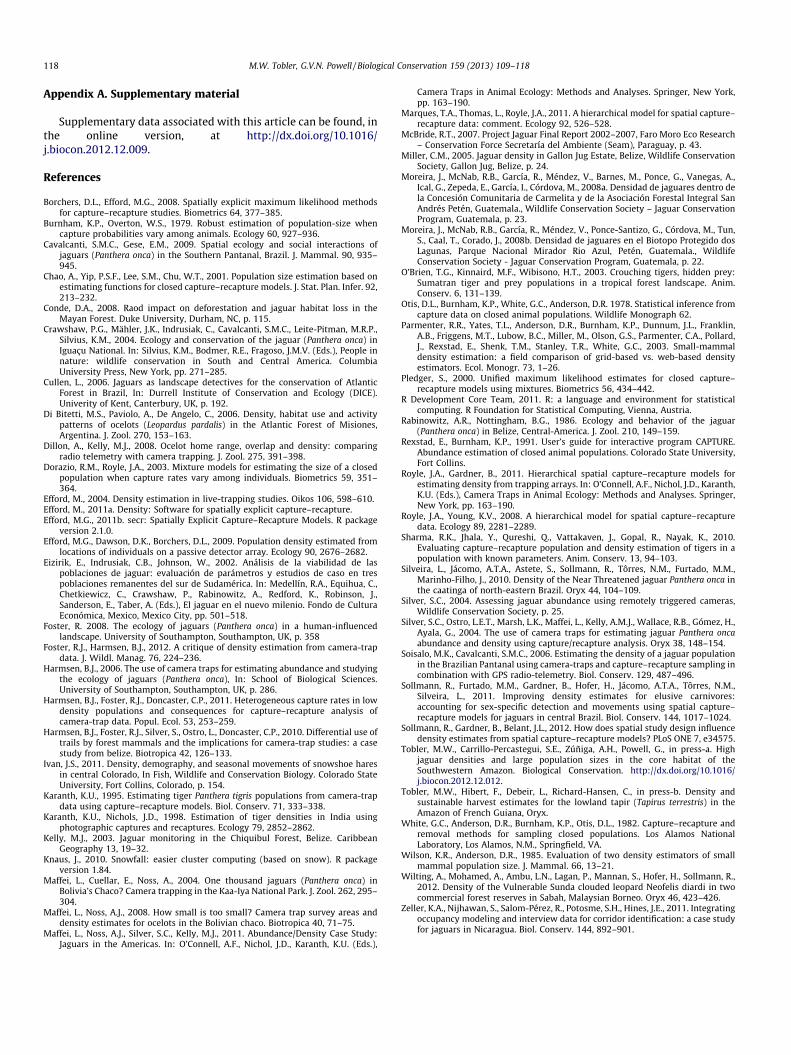
Appendix A. Design parameters and density estimates for camera trap surveys used to estimate jaguar (Panthera onca) densities. Densities are based on the Mh model and a buffer of ½ MMDM, which was the method most commonly used. In addition several studies also reported density estimates based on other methods. a Density estimates based on the Mh MMDM method b Density estimates based on a spatially explicate capture-recapture (SECR) model c Approximate density estimate not based on capture-recapture method Country Survey Statio

ns (N)

Days

Spacing (km)

Polygon (km2)

Captures (N)

Estimate (N)

MMDM (km)

Area 1/2 MMDM (km2)

Density ½ MMDM (Ind. 100 km-2)

Reported density (Ind. 100 km-2)

Reference

Argentina Iguazu 2004 39 45 2 209 4 5±1.41 11.33±2.7

576 1.07±0.33 0.49±0.16a (Paviolo et al. 2008)

Argentina Iguazu 2006 47 45 2.6 555 11 14±2.45

11.33±2.7

958 1.46±0.34 0.93±0.2a (Paviolo et al. 2008)

Argentina Urugua-i 34 45 1.25 81 1 - 11.33±2.7

368 0.3c 0.12a (Paviolo et al. 2008)

Argentina Yaboti 42 45 2.43 549 2 - 11.33±2.7

1001 0.2c 0.11a (Paviolo et al. 2008)

Belize Cockcomb basin 20 59 2.5 80 11 14±3.57

3.9±2.36 159 8.8±2.25 (Silver et al. 2004)

Belize Cockcomb basin 80 - - 322 11 unknown, in (Maffei et al. 2011) Belize Cockcomb basin 2002 20 59 2.5 80 11 14±3.5

7 3.9±2.36 159 8.8±3.69 (Harmsen 2006)

Belize Cockcomb basin 2003 19 65 2.5 80 9 10±1.53

5.62±1.04

207 4.82±0.96 (Harmsen 2006)


4.78±0.88

191 18.29±5.21 (Harmsen 2006)


4.58±1.08

183 11.45±5.54 (Harmsen 2006)

Belize Cockcomb basin 2005 17 62 130 - - - (Foster 2008) Belize Cockcomb basin 2006 13 62 79 - - - (Foster 2008) Belize Cockcomb basin 2007 21 40 165 - - - (Foster 2008) Belize Cockcomb basin 2008 44 62 290 - - - (Foster 2008) Belize Chiquibul 15 27 2.5 89 7 8±2.51 3.1±1.62 107 7.48±2.74 (Silver et al. 2004) Belize Fireburn 16 63 3 55 5 7 5.2 132 5.3±1.76 (Miller 2006) Belize Gallon Jug Estate 2004 28 62 2.5 105 15 6.9 195 11.28±2.66 (Miller 2005) Belize Gallon Jug Estate 2005 24 62 2.5 95 12 22 5.06 170 8.82±2.27 (Miller 2005) Belize Mountain Pine Ridge 80 105 - - 302 2.32 M. Kelly unpubl. data, in (Maffei et

al. 2011)

Belize Mountain Pine Ridge 64 140 - - 345 5.35 M. Kelly unpubl. data, in (Maffei et al. 2011)

Bolivia Cerro Cortado I Kaa-Iya

38 60 1.7 49 7 7±3.01 4.82±2.24

137 5.11±2.1 (Silver et al. 2004)

Bolivia Cerro Cortado II Kaa-Iya

28 60 2.5 52 7 8 5.62 149 5.37±1.79 (Maffei et al. 2004)

Bolivia El Encanto 20 60 2 36 4 6 0.97 106 5.66±2.33 (Arispe et al. 2007) Bolivia Estacion Isoso I, Kaa-

Iya 2005 22 56 3.5 48 4 5±1.59 6.6 158 3.16±1.17 (Maffei et al. 2006)

Bolivia Estacion Isoso II, Kaa-Iya 2006

20 64 3.5 51 4 6±3.18 5.99 153 3.93±0.27 (Romero-Muñoz et al. 2007)

Bolivia Guanaco, Kaa-Iya I 16 60 3 49 5 5±0.35 9.2 243 2.05±0.21 (Cuéllar et al. 2004a) Bolivia Guanaco, Kaa-Iya II 18 60 3 62 4 4±0.35 6.26 191 2.09±0.45 (Cuéllar et al. 2004b) Bolivia Palmar I, Kaa-Iya 2006 23 61 2 72 3 3±0.03

5 7.6 230 1.32 (Romero-Muñoz et al. 2006)

Bolivia Palmar II, Kaa-Iya 434 - - 1058 1.13±0.13 (Montaño et al. 2007) Bolivia Ravelo I, Kaa-Iya 36 60 2.5 100 5 7 7.88 309 2.27±0.89 (Maffei et al. 2004) Bolivia Ravelo II, Kaa-Iya 2.5 100 5 7 8.2 319 1.57 (Cuéllar et al. 2003) Bolivia Rios Tuichi and Hondo,

Madidi 66 28 2.5 200 9 13±8.1

6 7.1±2.8 458 2.84±1.78 (Silver et al. 2004)

Bolivia Rios Tuichi and Hondo, Madidi

45 30 54 - 1.6 127 - (Wallace et al. 2003)

Bolivia Rios Tuichi and Hondo, Madidi

32 29 77 - - 170 1.68±0.78 (Wallace et al. 2003)

Bolivia San Miguelito 28 60 1.5 24 5 6±1.54 2.8 54 11 (Rumiz et al. 2003) Bolivia San Miguelito 25 60 1.5 54 6 6±1.57 5.1 142 4.23±1.43 (Arispe et al. 2005) Bolivia Tucavaca I, Kaa-Iya 32 60 1.7 130 7 7±2.63 5.98±1.7

8 272 2.57±0.77 (Silver et al. 2004)

Bolivia Tucavaca II, Kaa-Iya 16 60 2.5 49 4 4 4.6 128 3.1±97 (Maffei et al. 2004) Brazil Emas National Park 62 1.5 - - 500 2 (Silveira 2004) Brazil Emas National Park 119 85 3.5 1320 10 - 10 1,750 0.51±0.19 0.29±0.10b (Sollmann et al. 2011) Brazil Fazenda Santa Fe 80 - - 425 2.59±1.03 L. Silveira and N.M. Negrões, in

(Maffei et al. 2011) Brazil Fazenda Sete 2003 42 20 165 31 37±5.5

2 6 360 10.3±1.53 5.7±0.84a (Soisalo and Cavalcanti 2006)

Brazil Fazenda Sete 2004 16 60 110 25 32±5.53

5.8 274 11.7±1.94 5.8±0.97a (Soisalo and Cavalcanti 2006)

Brazil Moro do Diablo 73 20 6 330 10 13±2.46

13.74 526 2.47±0.46 (Cullen 2006)

Brazil Serra da Capivara 20 84 2.9 157 12 14±3.643

9.9±3.86 524 2.67±1.06 1.28±0.62a (Silveira et al. 2010)

Colombia Amacayacu 32 - - 120 4.2 (Payan 2009) Colombia Calderon river valley 70 - - 242 2.5 (Payan 2009) Costa Rica Corcovado 11 30 2.75 29 4 6±1.96 3.48±0.4

7 86 6.98±2.36 (Salom-Perez et al. 2007)

Costa Rica Golfo Dulce / Golfito 134 35 1 102 4 5±0.71 9.04 218 2±1.49 (Bustamante 2008)

Costa Rica San Cristobal 15 43 2.3 50 4 9±11.9 3.48 134 6.7 (Rojas 2006) Costa Rica Talamanca 24 30 1.75 85 4 4±0.3 9.2 298 1.34±0.48 (Gutiérez and Porras 2008) Costa Rica Talamanca ZPLT

(Coton) 10 60 1.5 19 4 5±2.12 5.77 92 5.42±2.3 2.25a (Gonzáles-Maya 2007)

Ecuador Yasuni-Waorani 94 - - 218 1.38±0.6 S. Espinoza unpubl. data, in (Maffei et al. 2011)

Ecuador Yasuni ITT 32 64 2.5 58 4 4±2.62 6 182 2.2 (Araguillin et al. 2010) French Guiana

Counami Forest 19 90 2.5 60 6 8 - 242 3.3 (Association Kwata 2009)

French Guiana

Montagne de Fer 19 90 2.5 70 9 10 6.63 204 4.9 (Association Kwata 2009)

Guatemala Carmelita-AFISAP 20 45 2.5 51 10 13±2.6 4.24 115 11.28±3.51 (Moreira et al. 2008a) Guatemala La Gloria-Lechugal 33 46 2.5 128 6 6±2.59 7.22 390 1.54±0.85 (Moreira et al. 2007) Guatemala Mirador, Oeste 33 47 2 94 7 7±0.82 9.87 351 1.99±1.57 0.9±0.48a (Moreira et al. 2005) Guatemala Dos Lagunas Rio Azul 25 47 2.5 39 6 - 5.84 76 11.14±7.45 7.02±6.44a (Moreira et al. 2008b) Guatemala Tikal 15 34 39 7 8±3.01

5 4.52±4.14

121 6.63±2.46 3.39a (García et al. 2006)

Guatemala Melchor de Mecos 23 45 2 67 9 12±2.63

6.5 199 6.04±1.68 2.91±0.72a (Moreira et al. 2010)

Guatemala Laguna del Tigre 24 49 2.5 55 9 10±1.23

4.4 158 6.32±1.66 3.73±0.49a (Moreira et al. 2009)

Honduras La Mosquitia 20 60 0.8 20 5 5 2.87 96 5.2c (Portillo Reyes and Hernández 2011)

Mexico Sonora 26 60 3.5 100 5 - - 140 1±1.3c (Rosas-Rosas 2006) Mexico San Luis Potosi 2007 13 81 1.5 61 3 3±1.22 - 70 - (Avila Nájera 2009) Mexico San Luis Potosi 2008 27 31 1.5 53 3 5±1.93 5.672 156 3.2±1.9 1.55±1.93a (Avila Nájera 2009) Panama Darian 23 35 2.2 67 3 4±5.1 8 213 1.87 0.71a (Moreno 2006) Panama Darian 22 50 3.2 110 4 12±5.8 5.7 274 4.38 2.69a (Moreno 2006) Peru Los Amigos 2005 24 62 2 56 9 13±3.6

9 3.987 130 10.1±2.04 (Tobler et al. submitted)

Peru Los Amigos 2006 40 62 2 56 10 10±2.56

4.521±0.907

141 7.13±2.05 4.5±1.4b (Tobler et al. submitted)

Peru Los Amigos 2007 40 62 2 56 12 15±2.57

3.343±0.561


Peru Bahuaja Sonene, Tambopata

43 62 2 52 6 9±3.56 3.155±0.951

105 8.1±3.6 (Tobler et al. submitted)

Peru Espinoza 38 122 3 250 26 36±6.26

7.569±1.154


Araguillin, E., G. Z. Ríos, V. Utreras, and A. Noss. 2010. Muestreo con trampas fotográficas de mamíferos medianos, grandes y de aves en el

Bloque Ishpingo Tambococha Tiputini (ITT), sector Varadero (Parque Nacional Yasuní). Wildlife Conservation Society Ecuador, Quito, Ecuador.

Arispe, R., D. Rumiz, and C. Venegas. 2005. Segundo censo de jaguares (Panthera onca) y otros mamíferos con trampas-cámara en la estancia San Miguelito, Santa Cruz, Bolivia. Wildlife Conservation Society, Santa Cruz, Bolivia.

Arispe, R., D. Rumiz, and C. Venegas. 2007. Censo de jaguares (Panthera onca) y otros mamíferos con trampas cámara en la Concesión Forestal El Encanto. Wildlife Conservation Society, Santa Cruz, Bolivia.

Association Kwata. 2009. Camera-traps for survey of felids in French Guiana 2007-2008. Association Kwata, Cayenne, French Guiana. Avila Nájera, D. M. 2009. Abundancia del Jaguar (Panthera onca) y de sus Presas en el Municipio de Tamasopo, San Luis Potosí. M.Sc. Thesis.

Instituto de Enseñanzas e Investigacion en Ciencias Agricolas, Montecillo, Mexico. Bustamante, A. H. 2008. Densidad y uso de hábitat por los felinos en la parte sureste del área de amortiguamiento del Parque Nacional

Corcovado, Península de Osa, Costa Rica. M.Sc. Thesis. Universidad Nacional, Heredia, Costa Rica. Cuéllar, E., T. Dosapei, R. Peña, and A. Noss. 2003. Jaguar and other mammal camera trap survey Ravelo II, Ravelo field camp (19° 17’ 44” S,

60° 37’ 10” w) Kaa-Iya del Gran Chaco National Park. 18 September - 18 November 2003. Wildlife Conservation Society, Santa Cruz, Bolivia.

Cuéllar, E., J. Segundo, G. Castro, J. Barrientos, Juliet Healy, A. Hesse, and A. Noss. 2004a. Jaguar and other mammal camera trap survey Guanaco area (20° 03’ 03” s, 62° 26’ 04” w) Kaa-Iya del Gran Chaco National Park. 19 December 2003– 16 February 2004. Wildlife Conservation Society, Santa Cruz, Bolivia.

Cuéllar, E., J. Segundo, G. Castro, A. Segundo, A. Hesse, and A. Noss. 2004b. Jaguar and other mammal camera trap survey Guanaco II (20° 03’ 03” S, 62° 26’ 04” W) Kaa-Iya del Gran Chaco National Park. 18 August - 18 October 2004. Wildlife Conservation Society, Santa Cruz, Bolivia.

Cullen, L. 2006. Jaguars as landscape detectives for the conservation of Atlantic Forest in Brazil. Univerity of Kent, Canterbury, UK. Foster, R. 2008. The ecology of jaguars (Panthera onca) in a human-influenced landscape. Ph.D. Dissertation. University of Southampton,

Southampton, UK. García, R., R. B. McNab, J. S. Shoender, J. Radachowsky, J. Moreira, C. Estrada, V. Méndez, D. Juárez, T. Dubón, M. Córdova, F. Córdova, F.

Oliva, G. Tut, K. Tut, E. González, E. Muñoz, L. Morales, and L. Flores. 2006. Los jaguares del corazón del Parque Nacional Tikal, Petén, Guatemala. Wildlife Conservation Society-Programa para Guatemala, Guatemala.

Gonzáles-Maya, J. F. 2007. Densidad, uso de hábitat y presas del jaguar (Panthera onca) y el conflicto con humanos en la región de Talamanca, Costa Rica. M.Sc. Thesis. Centro Agronomico Tropical de Investigación y Enseñanza, Turrialba, Costa Rica.

Gutiérez, D. C. and J. C. Porras. 2008. Ecolgía poblacional de jaguar (Panthera onca) y puma (Puman concolor) y dieta de jaguar, en el sector Pacífico de la Cordillera de Talamanca, Costa Rica. B.Sc. Thesis. Universidad Latina de Costa Rica, San José, Costa Rica.

Harmsen, B. J. 2006. The use of camera traps for estimating abundance and studying the ecology of jaguars (Panthera onca). Ph.D. Dissertation. University of Southampton, Southampton, UK.

Maffei, L., E. Cuellar, and A. Noss. 2004. One thousand jaguars (Panthera onca) in Bolivia's Chaco? Camera trapping in the Kaa-Iya National Park. Journal of Zoology 262:295-304.

Maffei, L., A. J. Noss, S. C. Silver, and M. J. Kelly. 2011. Abundance/Density Case Study: Jaguars in the Americas. Pages 163-190 in A. F. O'Connell, J. D. Nichol, and K. U. Karanth, editors. Camera Traps in Animal Ecology: Methods and Analyses. Springer, New York.

Maffei, L., R. Paredes, F. Aguanta, and A. Noss. 2006. Muestreo con trampas cámaras de jaguares y otros mamíferos en la estación Isoso (18° 25’ s, 61° 46’ w) Parque Nacional Kaa Iya del Gran Chaco. 28 de octubre – 24 de diciembre. Wildlife Conservation Society - Fundacion Kaa-Iya, Santa Cruz, Bolivia.

Miller, C. M. 2005. Jaguar density in Gallon Jug Estate, Belize. Wildlife Conservation Society, Gallon Jug, Belize. Miller, C. M. 2006. Jaguar density in Fireburn, Belize. Wildlife Conservation Society, Belize. Montaño, R., L. Maffei, and A. Noss. 2007. Segundo muestreo con trampas cámaras de jaguares y otros mamíferos en el Campamento Palmar

de las Islas y Ravelo (Diciembre 2006–Marzo 2007). Wildlife Conservation Society, Santa Cruz, Bolivia. Moreira, J., R. García, R. McNab, G. P. Santizo, M. Mérida, V. Méndez, G. Ruano, M. Córdova, F. Córdova, Y. López, E. Castellanos, R.

Lima, and M. Burgos. 2010. Abundancia de jaguares y evaluación de presas asociadas al fototrampeo en las Concesiones Comunitarias del Bloque de Melchor de Mencos, Reserva de la Biosfera Maya, Petén, Guatemala. Wildlife Conservation Society-Programa para Guatemala, Guatemala.

Moreira, J., R. García, R. B. McNab, G. Ruano, G. Ponce, M. Mérida, K. Tut, P. Díaz, E. González, M. Córdova, E. Centeno, C. López, A. Vanegas, Y. Vanegas, F. Córdova, J. Kay, G. Polanco, and M. Barnes. 2005. Abundancia de jaguares y presas asociadas al fototrampeo en el sector oeste del Parque Nacional Mirador - Río Azul, Reserva de Biosfera Maya. Wildlife Conservation Society-Programa para Guatemala, Guatemala.

Moreira, J., R. McNab, R. García, G. Ponce, M. Mérida, V. Méndez, M. Córdova, G. Ruano, K. Tut, H. Tut, F. Córdova, E. Muñoz, E. González, J. Cholom, and A. Xol. 2009. Abundancia y densidad de jaguares en el Parque Nacional Laguna del Tigre-Corredor Biológico Central, Reserva de la Biosfera Maya. Wildlife Conservation Society-Programa para Guatemala, Guatemala.

Moreira, J., R. B. McNab, R. García, V. Méndez, M. Barnes, G. Ponce, A. Vanegas, G. Ical, E. Zepeda, I. García, and M. Córdova. 2008a. Densidad de jaguares dentro de la Concesión Comunitaria de Carmelita y de la Asociación Forestal Integral San Andrés Petén, Guatemala., Wildlife Conservation Society - Jaguar Conservation Program, Guatemala.

Moreira, J., R. B. McNab, R. García, V. Méndez, G. Ponce-Santizo, M. Córdova, S. Tun, T. Caal, and J. Corado. 2008b. Densidad de jaguares en el Biotopo Protegido dos Lagunas, Parque Nacional Mirador Rio Azul, Petén, Guatemala., Wildlife Conservation Society - Jaguar Conservation Program, Guatemala.

Moreira, J., R. B. McNab, D. Thornton, R. García, V. Méndez, A. Vanegas, G. Ical, E. Zepeda, R. Senturión, I. García, J. Cruz, G. Asij, G. Ponce, J. Radachowsky, and M. Córdova. 2007. Abundancia de jaguares en La Gloria-El Lechugal, Zona de Usos Múltiples, Reserva de la Biosfera Maya, Petén, Guatemala. Wildlife Conservation Society-Programa para Guatemala, Guatemala.

Moreno, R. S. R. 2006. Parámetros poblacionales y aspectos ecológicos de los felinos y sus presas en Cana, Parque Nacional Darien, Panamá. M.Sc. Thesis. Universidad Nacional, Heredia, Costa Rica.

Paviolo, A., C. D. de Angelo, Y. E. Di Blanco, and M. S. Di Bitetti. 2008. Jaguar Panthera onca population decline in the Upper Parana Atlantic Forest of Argentina and Brazil. Oryx 42:554-561.

Payan, E. C. G. 2009. Hunting sustainability, species richness and carnivore conservation in Colombian Amazonia. Ph.D. Dissertation. University College London, London, UK.

Portillo Reyes, H. O. P. and J. Hernández. 2011. Densidad del jaguar (Panthera onca) en honduras: primer estudio con trampas-cámara en la Mosquitia Hondureña. Revista Latinoamericana de Conservación 2:45-50.

Rojas, R. A. 2006. El jaguar (Panthera onca) en el sector San Christobal del Área de Conservación Guanacaste-Costa Rica:densidad, abundancia de presas y depredación de ganado. M.Sc. Thesis. Universidad Nacional, Heredia, Costa Rica.

Romero-Muñoz, A., R. Montaño, R. Peña, T. Dosapey, and R. Paredes. 2006. Muestreo con trampas cámara de jaguares y otros mamíferos en el Campamento Palmar de las Islas (19º 25’ S, 60º 32’ O) 6 de marzo – 6 de junio 2006. Wildlife Conservation Society, Santa Cruz, Bolivia.

Romero-Muñoz, A., R. Paredes, and L. Maffei. 2007. Segundo muestreo con trampas cámaras de jaguares y otros mamíferos en la estación Isoso (18° 25’ s, 61° 46’ w) Parque Nacional Kaa Iya del Gran Chaco.7 de Julio – 8 de Septiembre, 2006. Wildlife Conservation Society - Fundacion Kaa-Iya, Santa Cruz, Bolivia.

Rosas-Rosas, O. C. 2006. Ecological status and conservation of jaguars (Panthera onca) in northeastern Sonora, Mexico. Ph.D. Dissertation. New Mexico State University, Las Cruces, New Mexico.

Rumiz, D. I., R. Arispe, A. J. Noss, and K. Rivero. 2003. Censo de jaguares (Panthera onca) y otros mamíferos con trampas-cámara en la estancia San Miguelito, Santa Cruz, Bolivia. Wildlife Conservation Society, Santa Cruz, Bolivia.

Salom-Perez, R., E. Carrillo, J. C. Saenz, and J. M. Mora. 2007. Critical condition of the jaguar Panthera onca population in Corcovado National Park, Costa Rica. Oryx 41:51-56.

Silveira, L. 2004. Ecologia comparada e conservação da onça-pintada (Panthera onca) e onça-parda (Puma concolor), no Cerrado e Pantanal. Ph.D. Dissertation. Universidade de Brasília, Brasilia, Brazil.

Silveira, L., A. T. A. Jácomo, S. Astete, R. Sollmann, N. M. Tôrres, M. M. Furtado, and J. Marinho-Filho. 2010. Density of the Near Threatened jaguar Panthera onca in the caatinga of north-eastern Brazil. Oryx 44:104-109.

Silver, S. C., L. E. T. Ostro, L. K. Marsh, L. Maffei, A. M. J. Kelly, R. B. Wallace, H. Gómez, and G. Ayala. 2004. The use of camera traps for estimating jaguar Panthera onca abundance and density using capture/recapture analysis. Oryx 38:148-154.

Soisalo, M. K. and S. M. C. Cavalcanti. 2006. Estimating the density of a jaguar population in the Brazilian Pantanal using camera-traps and capture-recapture sampling in combination with GPS radio-telemetry. Biological Conservation 129:487-496.

Sollmann, R., M. M. Furtado, B. Gardner, H. Hofer, A. T. A. Jácomo, N. M. Tôrres, and L. Silveira. 2011. Improving density estimates for elusive carnivores: Accounting for sex-specific detection and movements using spatial capture-recapture models for jaguars in central Brazil. Biological Conservation 144:1017-1024.

Tobler, M. W., S. E. Carrillo-Percastegui, A. H. Zúñiga, and G. Powell. submitted. High jaguar densities and large population sizes in the core habitat of the Southwestern Amazon. Biological Conservation.

Wallace, R. B., H. Gomez, G. Ayala, and F. Espinoza. 2003. Camera trapping for jaguar (Panthera onca) in the Tuichi Valley, Bolivia. Journal of Neotropical Mammology 10:133-139.

Appendix B. Summary of published home range estimates for the jaguar (Panthera onca). MCP: minimum convex polygon, KHR: kernel home range, HM: harmonic mean. Female Home Range (km2) Male Home Range (km2) Country Habitat N min max mean N min max mean Estimator Telemetry Comments Reference Belize Moist forest 1 11 4 28 40 33 MCP VHF females based on tracks (Rabinowitz and Nottingham 1986) Brazil Atlantic forest 5 18 192 92 2 89 471 280 KHR 95% VHF (Cullen 2006) Brazil Atlantic forest 2 135 289 212 1 299 KHR 95% VHF (Cullen 2006) Brazil Moist forest 2 8 70 39 7 5 138 57 MCP VHF very few locations (Crawshaw et al. 2004) Brazil Pantanal 4 30 83 57 6 72 231 152 MCP 98% GPS Wet season (Cavalcanti and Gese 2009) Brazil Pantanal 4 40 97 69 6 73 268 170 MCP 98% GPS Dry season (Cavalcanti and Gese 2009) Brazil Pantanal 4 34 89 62 6 83 197 140 KHR 90% GPS Wet season (Cavalcanti and Gese 2009) Brazil Pantanal 4 40 87 63 6 73 258 165 KHR 90% GPS Dry season (Cavalcanti and Gese 2009) Brazil Pantanal 4 97 168 139 1 152 MCP VHF (Crawshaw and Quigley 1991) Brazil Pantanal 1 193 3 253 472 337 HM 95% VHF Harmonic mean HR (Silveira 2004) Brazil Pantanal 38 67 KHR 95% VHF (de Azevedo and Murray 2007) Brazil Pantanal 1 34 VHF (Schaller and Crawshaw 1980) Mexico Deciduous dry forest 2 60 MCP? VHF (Núñez et al. 2000) Mexico Moist forest 2 31 59 45 2 33 40 36 VHF (Ceballos et al. 2002) Mexico Moist forest 122 293 280 970 MCP GPS (Conde 2008) Paraguay Chaco 2 388 492 440 3 390 1291 692 KHR GPS Probably KHR 95% (McBride 2007) Paraguay Pantanal 2 69 72 70 KHR GPS Probably KHR 95% (McBride 2007) Venezuela Llanos 1 83 2 93 108 100 KHR 95% VHF Dry season (Scognamillo et al. 2003) Venezuela Llanos 2 47 66 56 0 KHR 95% VHF Wet season (Scognamillo et al. 2003)

References Cavalcanti, S. M. C. and E. M. Gese. 2009. Spatial Ecology and social interactions of jaguars (Panthera onca) in the Southern Pantanal, Brazil.

Journal of Mammalogy 90:935-945. Ceballos, G., C. Chavez, A. Rivera, C. Manterola, and B. Wall. 2002. Tamaño poblacional y conservación del jaguar en la reserva de la biosefera

Calakmul, Campeche, México. Pages 403-417 in R. A. Medellín, C. Equihua, C. Chetkiewicz, P. Crawshaw, A. Rabinowitz, K. Redford, J. Robinson, E. Sanderson, and A. Taber, editors. El jaguar en el nuevo milenio. Fondo de Cultura Económica, Mexico City, Mexico.

Conde, D. A. 2008. Raod impact on deforestation and jaguar habitat loss in the Mayan Forest. Ph.D. Dissertation. Duke University, Durham, NC. Crawshaw, P. G., J. K. Mähler, C. Indrusiak, S. M. C. Cavalcanti, M. R. P. Leite-Pitman, and K. M. Silvius. 2004. Ecology and Conservation of

the Jaguar (Panthera onca) in Iguaçu National. Pages 271-285 in K. M. Silvius, R. E. Bodmer, and J. M. V. Fragoso, editors. People in nature : wildlife conservation in South and Central America. Columbia University Press, New York.

Crawshaw, P. G. and H. B. Quigley. 1991. Jaguar Spacing, Activity and Habitat Use in a Seasonally Flooded Environment in Brazil. Journal of Zoology 223:357-370.

Cullen, L. 2006. Jaguars as landscape detectives for the conservation of Atlantic Forest in Brazil. Univerity of Kent, Canterbury, UK. de Azevedo, F. C. C. and D. L. Murray. 2007. Spatial organization and food habits of jaguars (Panthera onca) in a floodplain forest. Biological

Conservation 137:391-402. McBride, R. T. 2007. Project Jaguar Final Report 2002 - 2007. Faro Moro Eco Research – Conservation Force Secretaría del Ambiente (Seam),

Paraguay. Núñez, R., B. Miller, and F. Lindzey. 2000. Food habits of jaguars and pumas in Jalisco, Mexico. Journal of Zoology 252:373-379. Rabinowitz, A. R. and B. G. Nottingham. 1986. Ecology and behavior of the jaguar (Panthera onca) in Belize, Central-America. Journal of

Zoology 210:149-159. Schaller, G. B. and P. G. Crawshaw. 1980. Movement patterns of jaguar. Biotropica 12:161-168. Scognamillo, D., I. E. Maxit, M. Sunquist, and J. Polisar. 2003. Coexistence of jaguar (Panthera onca) and puma (Puma concolor) in a mosaic

landscape in the Venezuelan llanos. Journal of Zoology 259:269-279. Silveira, L. 2004. Ecologia comparada e conservação da onça-pintada (Panthera onca) e onça-parda (Puma concolor), no Cerrado e Pantanal.

Ph.D. Dissertation. Universidade de Brasília, Brasilia, Brazil.

Appendix C. Additional graphs for different parameter combinations.

Coefficient of variation of the density (standard error / mean) in relationship to the number of captured individuals for simulated capture-recapture analyzed with a spatially explicit capture-recapture (SECR) model. The data shown combine simulation runs with the following parameters: grid size=403 km2, λ0 (0.05,0.1), number of cameras (36,49,64), number of occasions (30, 60, 90), simulated density (1, 2, 4 ind. 100 km-2), home range=400 km2 (σ=4592).

10 20 30 40 50 60

0.0

0.5

1.0

1.5

2.0

2.5

Individuals

Coe

ffici

ent o

f Var

iatio

n

Coefficient of variation of the density (standard error / mean) in relationship to the number of captured individuals for simulated capture-recapture analyzed with the Mh full MMDM method. The data shown combine simulation runs with the following parameters: grid size=403 km2, λ0 (0.05,0.1), number of cameras (36,49,64), number of occasions (30, 60, 90), simulated density (1, 2, 4 ind. 100 km-2), home range=400 km2 (σ=4592).

10 20 30 40 50 60

0.0

0.5

1.0

1.5

2.0

2.5

Individuals

Coe

ffici

ent o

f Var

iatio

n

Bias of densities estimated by the Mh full MMDM method in relation to different densities and camera trap survey parameters for simulated jaguar capture-recapture (analog to Figure 4 in the main article). The graph shows the distribution of the bias from 110 simulation runs for each parameter combination. The bottom and top of the box show the 25th and 75th percentiles, respectively, the horizontal line indicates the median and the whiskers show the range of the data except for outlier indicated by circles. St.: camera station.

Mean bias of densities estimated by the Mh full MMDM method in relation to different camera grid shapes for simulated jaguar capture-recapture data (analog to Figure 5 in the main article). The data shown combines simulation runs with the following parameters: λ0=0.01, home range=400 km2 (σ=4592), number of occasions=60, simulated density (2, 4).

Den

sity

Bia

s (%

)

Hom

e R

ange

150

km2 , P

olyg

on 1

48 km

2

-100

010

020

030

040

050

060

Den

sity

Bia

s (%

)

Hom

e R

ange

400

km2 , P

olyg

on 4

03 km

2

Density 1 ind. 100 km2

36 St.30 d

36 St.90 d

49 St.60 d

64 St.30 d

64 St.90 d

-100

010

020

030

040

050

060

0


36 St.30 d

36 St.90 d

49 St.60 d

64 St.30 d

64 St.90 d


36 St.30 d

36 St.90 d

49 St.60 d

64 St.30 d

64 St.90 d


Den

sity

Bia

s (%

)

33 55 90 148 245 403 665 1097 1808 2981 4915 8103 13360

020

4060

8010

013

0

7 x 75 x 104 x 122 x 24

Bias of densities estimated by a spatially explicit capture-recapture model (SECR) for two different grid shapes (a) 7 x 7 cameras, (b) 3 x 16 cameras. The data shown combines simulation runs with the following parameters: λ0=0.01, home range=400 km2 (σ=4592), number of occasions 60, simulated density (2, 4). The bottom and top of the box show the 25th and 75th percentiles, respectively, the horizontal line indicates the median and the whiskers show the range of the data except for outlier indicated by circles.

010

020

030

0

b

33 55 90 148 245 403 665 1097 1808 2981 4915 8103

010

020

030

0

b

Trap Polygon (km2)

Den

sity

Bia

s (%

)

Correction of bias by small camera polygons by fixing MMDM to the true value for the Mh full MMDM method (analog to Figure 7 in the main article). (a) MMDM estimated by from data and full MMDM used for density etimstes, (b) MMDM set to the true simulated value and ½ MMDM used for density estimates. The following simulation parameters were used: λ0=0.01, number of cameras=49, number of occasions=60, simulated density (2, 4 ind. 100 km-2), home range=400 km2 (σ=4592). The bottom and top of the box show the 25th and 75th percentiles, respectively, the horizontal line indicates the median and the whiskers show the range of the data except for outlier indicated by circles.

010

020

030

0

a

33 55 90 148 245 403 665 1097 1808 2981 4915 8103 13360

010

020

030

0

b


Den

sity

Bia

s (%

)

Estimating jaguar densities with camera traps:...

Documents

Transcript of Estimating jaguar densities with camera traps:...