1

Estimating Extended Supply-Use Tables in Basic Prices with Firm

Heterogeneity for the United States:

A Proof of Concept

James J. Fetzer, Thomas F. Howells III, Lin Z. Jones, Erich H. Strassner, and Zhi Wang1

This paper presents proof-of-concept trade-in-value added (TiVA) statistics estimated from extended supply-use tables for the United States that account for firm heterogeneity. The tables used to estimate the TiVA statistics extend recently-introduced supply-use tables for the United States by disaggregating the components of supply and use by multinational and other firms. Recent research has shown both the advantages of measuring trade on a value added basis when analyzing bilateral trade flows and the dominance of multinational enterprises in U.S. trade in goods and services. Our TiVA statistics for the United States include measures based on traditional supply-use presentations as well as statistics that reflect firm-level heterogeneity for the year 2011. The comparative analysis of the two sets of statistics allows us to understand better how firms within industries engage in global value chains and if the incorporation of firm heterogeneity provides a more accurate measurement of TiVA. We find that domestic value added as a share of the value of exports is similar within large industry groups. However, there is much more variation in the value added share of exports when firm type is accounted for. Also, the additional granularity shows the share of this value added that comes directly from the producing industry varies much more across industries.

1 Fetzer, Howells, and Strassner are at the Bureau of Economic Analysis, U.S. Department of Commerce

(James.Fetzer@bea.gov, Thomas.Howells@bea.gov, and Erich.Strassner@bea.gov). Jones is at the U.S. International Trade Commission (lin.jones@usitc.gov) and Wang is at the Schar School of Policy and Government at George Mason University and the Research Center of Global Value Chains at the University of International Business and Economics in Beijing (zwang36@gmu.edu). We thank Paul Farello, Ray Mataloni, Sally Thompson, David Wassahusen, and Robert Yuskavage for helpful comments and conversations. We thank Christopher Wilderman for his assistance on the tax data and on concordances between classification systems. The views expressed in this paper are those of the author and should not be attributed to the Bureau of Economic Analysis, U.S. Department of Commerce or the U.S. International Trade Commission.

1

1 Introduction

Pioneering work on measuring trade in value added (TiVA) began with efforts in

academia (e.g. Global Trade Analysis Project (GTAP)), in government (e.g. United States

International Trade Commission (USITC) and the World Input-Output Database (WIOD)), and in

international organizations (e.g. Organisation for Economic Co-operation (OECD) and World

Trade Organization). These initial efforts have raised the profile of TiVA and generated strong

demand for better understanding of how global value chains work, which has motivated

national statistical agencies to find ways to measure trade-in-value added (TiVA) more

accurately. Research has shown that a sizeable share of trade is composed of intermediate

goods that have crossed borders multiple times and that bilateral trade balances measured

using (TiVA) can be very different than the trade balances using gross trade flows (Johnson and

Noguera (2012)). These differences matter because they imply differences in competitiveness

vis-a-vis trading partners and their implications for trade policy.2

As noted by Fetzer and Strassner (2015) and others, national statistical agencies have

found direct measurement of TiVA to be impractical. Instead, efforts to measure TiVA more

accurately have focused on better refining supply-use tables (SUTs) that can be used to

measure the value added portion of trade indirectly by particular industries. Accurate

measurement of TiVA for a country using this method depends on the SUTs of all major trading

partners because the SUTs must be linked using bilateral trade flows. Improvements in these

2 See Dervis, Metzer and Foda (2013) “Value-Added Trade and Its Implications for Trade Policy”

http://www.brookings.edu/research/opinions/2013/04/02-implications-international-trade-policy-dervis-meltzer

2

tables have benefitted from international collaboration on issues such as the industry and

product classifications and valuations of these tables. These efforts have also aimed to extend

these tables by taking into account different dimensions of firm-level heterogeneity within

industries and challenging the historical assumption of a homogenous production function for

all firms within a given industry.

This paper builds on recently-published SUTs for the United States (Young, Howells,

Strassner, and Wasshausen 2015). We estimate “proof of concept” extended SUTs

disaggregated by firm type based on the methodology of Fetzer and Strassner (2015). These

tables foreshadow more precise estimates of extended SUTs that will be the product of an

ongoing long-term U.S. Bureau of Economic Analysis (BEA) - U.S. Census Bureau (Census)

microdata link project. We also estimate measures of TiVA based on the input-output

coefficients derived from these SUTs.

2 Literature Review

Our paper builds on research that has decomposed industry output by firm type,

estimated extended input-output tables (IOTs), and estimated TiVA indicators using a single

country IOT. Recent research such as Fetzer and Strassner (2015), Piacentini and Fortanier

(2015), Ahmad, Araujo, Lo Turco, and Maggioni (2013), and Ma, Wang, and Zhu (2015) have

found evidence of heterogeneity in value added and trade between foreign- and domestic-

owned enterprises in a broad group of countries including the United States, China, and many

European countries. Our paper estimates the components of output and value added for

3

multinational enterprises (MNEs) and non-MNEs for the United States based on the

methodology used in Fetzer and Strassner (2015).

We also build on the literature that uses firm characteristics and constrained

optimization to estimate IOTs by type of firm. Koopman, Wang, and Wei (2012) developed a

method that allows for computing IOTs that distinguish between processing and normal trade.

Ma, Wang, and Zhu (2015) extend this approach by distinguishing between Chinese exports by

foreign-invested enterprises and by Chinese-owned enterprises. We use this framework to

refine further the U.S. use table to include valuation at basic prices and to disaggregate the U.S.

SUT by firm type.

Most TiVA estimates are based on global IO tables, but it is possible to generate TiVA

estimates using a single country’s IO tables, under certain assumptions. Koopman, Wang, and

Wei (2014) indicate that gross exports can be decomposed into domestic content and foreign

content using a single country IOT if there is no trade in intermediate goods. Ma, Wang, and

Zhu (2015) note that single country models are limited to estimating the domestic content of

exports. The domestic content of exports may differ from the domestic value added in exports

since it may include domestic content that has been re-imported. Los, Timmer, and de Vries

(forthcoming) indicate that domestic value added in gross exports can be estimated from the

difference in reported gross domestic product (GDP) and hypothetical GDP estimated from a

single country IOT assuming the country does not export. However, they indicate that global

IOTs are required to decompose domestic value added by end use including the extent to which

4

it is absorbed abroad. The weakness of this approach is that the U.S. production structure and

IOT would be different if the country did not export.

3 Data

The 2011 SUTs for the United States are the foundation on which the proof-of-concept

extended SUTs were constructed. The supply-use framework comprises two tables. The supply

table presents the total domestic supply of goods and services from both domestic and foreign

producers that are available for use in the domestic economy. The use table shows the use of

this supply by domestic industries as intermediate inputs and by final users as well as value

added by industry. The main part of each table is organized with industries across the columns

and commodities across the rows. The cells in the main part of the supply table indicate the

amount of each commodity (row) produced and/or used by an industry (column). The

remaining columns indicate the amount of each commodity that is imported and valuation

adjustments such as trade margins, transportation costs, taxes, and subsidies for each

commodity. The cells in the main part of the use table indicate the amount of a commodity

purchased as an intermediate input for an industry’s production process. The cells in the

remaining columns in the table indicate how each commodity is allocated to different

components of final demand. The cells in the bottom rows indicate how the components of

value added in an industry are allocated.3

3 Young, Howells, Strassner, and Wasshausen (2015).

5

The incorporation of BEA statistics on the Activities of Multinational Enterprises (AMNE)

is how firm heterogeneity is introduced into the SUTs and is what distinguishes them as

extended SUTs. These statistics cover the financial and operating characteristics of U.S. parent

companies (domestic-owned MNEs) and U.S. affiliates that are majority-owned by foreign

MNEs (foreign-owned MNEs). They are based on legally mandatory surveys conducted by the

BEA and are used in a wide variety of studies, such as this one, to estimate the impact of MNEs

on the domestic (U.S.) economy and on foreign host economies.

The tables presented here are part of a time series of SUTs, now covering the period

1997-2014, that were first released by the BEA in September of 2015.4 Release of these tables

marks an important milestone in BEA’s long-term plan to make U.S. data on output,

intermediate inputs, and value added available in a format that is well suited for preparation of

TiVA statistics.

With the September 2015 release, data previously presented only in the make-use

format were also presented in the more internationally recognized supply-use format.5

Presentation in this format will facilitate future efforts to link U.S. data with SUTs from other

countries, a step necessary to derive the full suite of TiVA-related statistics. In addition, the new

SUTs incorporate important valuation changes that bring the tables into better alignment with

international standards and enhance the suitability of the tables for use in TiVA analysis. First,

taxes in the new tables are separated into taxes on products and other taxes on production and 4 For a full discussion of the supply-use framework and the methodology followed by BEA to prepare the

new tables, see Young, Howells, Strassner, and Wasshausen (2015). 5 The new supply and use tables are supplemental products that will be produced in addition to, rather

than in place of, BEA’s current make and use tables.

6

output in the supply table, and value added in the use table is presented exclusive of taxes on

products (i.e. valued at basic prices). Second, a commodity distribution of customs duties on

imports is incorporated, and imports in the new tables are presented exclusive of duties (i.e.

valued at c.i.f.6).

Certain future enhancements to the SUTs are not reflected in the estimates presented

here. Currently, BEA is investigating the possibility of publishing tables on an International

Standard Industrial Classification (ISIC) basis. Additionally, BEA is investigating the possibility of

releasing a breakdown of the use tables valued at purchaser prices into their several

component matrices. This decomposition could include separate matrices for domestically-

produced inputs valued at basic prices, imported inputs at basic prices, margins, taxes on

products, and subsidies on products. These additions were not available for purposes of this

paper, so the tables were converted in a manner that approximates an ISIC basis and the

component matrices had to be estimated. The decomposition process is outlined in greater

detail in the methodology section and in appendix A.

The basic SUTs for 2011 are extended by incorporating data on firm-level heterogeneity

by industry. These data are prepared on an ISIC-basis for 33 industries following the

methodology used in Fetzer and Strassner (2015).7 As is the case in Fetzer and Strassner (2015),

we use 2011 IRS Statistics of Income (SOI) data to estimate value added by industry for all firms

with operations in the United States and BEA AMNE data for 2011. For U.S. MNEs, we 6 The c.i.f. valuation of imports refers to cost, insurance, and freight. This valuation includes the cost of

the import at the foreign port plus the insurance, freight charges, and charges other than import duties associated with transferring the import to the domestic port.

7 There is no BEA or IRS data for industry 34, “Private households with employed persons.”

7

separately analyze data for domestic-owned MNEs and for foreign-owned MNEs. Because of

some challenges working directly with the SOI data, we also use data from the BEA input-

output accounts to estimate exports and intermediate imports. However, unlike Fetzer and

Strassner (2015) we use the enterprise level SOI data on employee compensation and make

adjustments to implausible values on a case-by-case basis. We also match these data on an

ISIC-basis for 33 ISIC industries from the reported NAICS industries. This industry conversion is

necessary so that our tables are comparable to those produced by other OECD countries.

Results by industry for domestic non-MNEs are computed as the difference between the

SOI-based results for all U.S. firms less the results for directly measured domestic-owned and

foreign-owned MNEs. We use the SOI data instead of the BEA SUTs because the SOI data are

collected and published by industry at the enterprise level, similar to the BEA AMNE data.

The data for foreign MNEs, which are U.S. affiliates of foreign parent companies, are

generally reported as published by BEA except where imports or exports are suppressed to

protect the confidentiality of firms that make up most of the data in the industry and where

gross operating surplus, consumption of fixed capital, and taxes were not published for an

industry. In these cases, we estimate the share for each of these variables for all industries for

which the data are not reported or are suppressed and then impute a value from this aggregate

share.

The data for domestic-owned MNEs are adjusted by removing the MNEs that are

majority-owned by foreign parents to put the data on an ultimate U.S.-owner basis, just as the

8

foreign-owned MNE data are on an ultimate foreign-owner basis. Some industries had no

majority foreign-owned MNEs, so their data are the same as the regularly published data. We

impute data for several industries to protect the confidentiality of firms that make up a large

share of data for an industry. In these cases, we typically estimate the share of each variable

that needs to be imputed in the unadjusted data for all industries for which the data were not

reported or are suppressed and then impute a value from this aggregate share. One exception

is where we use unadjusted output shares to impute the imports and exports for industries

where the original unadjusted data were suppressed. Additionally, we reduce the trade data for

wholesale and retail trade for both domestic- and foreign-owned MNEs to better attribute the

trade to the using industries.8

We also make some adjustments to the SOI data to adjust for implausible values. Most

of the adjustments are made to employee compensation and to imports and exports, which in

total were based on the BEA SUTs. In particular we make large changes to values for

“Manufacturing not elsewhere classified and recycling.” The need to make large changes to

residual industry groups is typical because, by construction, these groups reflect measurement

error in all of the industry groups that are shown separately. There are no MNE data for public

administration and defense. We also assume that imports and exports were zero for public

administration and defense. Trade in both goods and services are included in the SOI data, but

only trade in goods is included in our MNE data. The BEA AMNE data include trade in services

and we are planning on incorporating this information along with information from our services

8 The adjustment is necessary because there is a wide body of evidence showing that wholesale

intermediaries play an important role in connecting imported products to using industries.

9

surveys in the future. Therefore our tables may attribute a disproportionate share of trade in

services to domestic-owned non-MNEs.

4 Methodology

We take several steps to prepare the extended SUTs and to derive TiVA estimates from

both the standard and extended SUTs. As mentioned in the previous section, a decomposition

of the use table at purchasers’ prices into its several component matrices is not currently

available. Therefore, we first estimate this decomposition using a quadratic programming

constrained optimization model and data from the published BEA SUTs. We then estimate an

extended SUT in which industries are broken down into different firm types. Following the

approach taken by Ma, Wang, and Zhu (2015), this is also done using a quadratic programming

constrained optimization model with estimates of the components of output by firm type

derived from BEA and IRS data. We use the resulting extended SUTs to construct a symmetric

industry-by-industry extended input-output table (IOT). Using the IOT, we calculate the Leontief

inverse from which are derived our TiVA statistics.

4.1 Decomposing the purchasers’ price use table and constructing extended SUTs

and IOTs

The international standard is for use table transactions to be valued at purchaser prices.

However, a basic price valuation is preferred for purposes of calculating TiVA statistics because

it ensures more homogenous valuation across different products, more accurately reflects a

country’s input-output relationships, and allows separate identification of the effects of import

10

tariffs, production taxes, and subsidies. Using a quadratic programming model with parameters

from BEA’s published SUTs, we decompose the purchaser price use table into separate matrices

for domestically-produced inputs valued at basic prices, imported inputs valued at basic prices,

margins, taxes on products, and subsidies on products. The model is detailed in Appendix A.

Following the decomposition of the purchaser price use table, we incorporate BEA and

IRS data on the components of output by firm type into the basic price SUT to construct

extended SUTs. We incorporate these data into the basic price SUT using an approach similar to

the constrained optimization model used by Ma, Wang, and Zhu (2015) for Chinese IOTs. We

estimate the share of output attributable to different types of firms: U.S.-owned MNEs, foreign-

owned MNEs, and non-MNEs. We then apply these shares to output of both primary and

secondary products and to taxes and margins in the supply tables to estimate the value of these

variables for each type of firm. Similarly, for the use table, we estimate the share of value

added attributable to each firm type from SOI and BEA data. We apply these shares to value

added in the use table. We then create a symmetric IOT from the SUTs for estimation of TiVA

statistics. The optimization model used for estimating extended SUTs is described in detail in

appendix B.

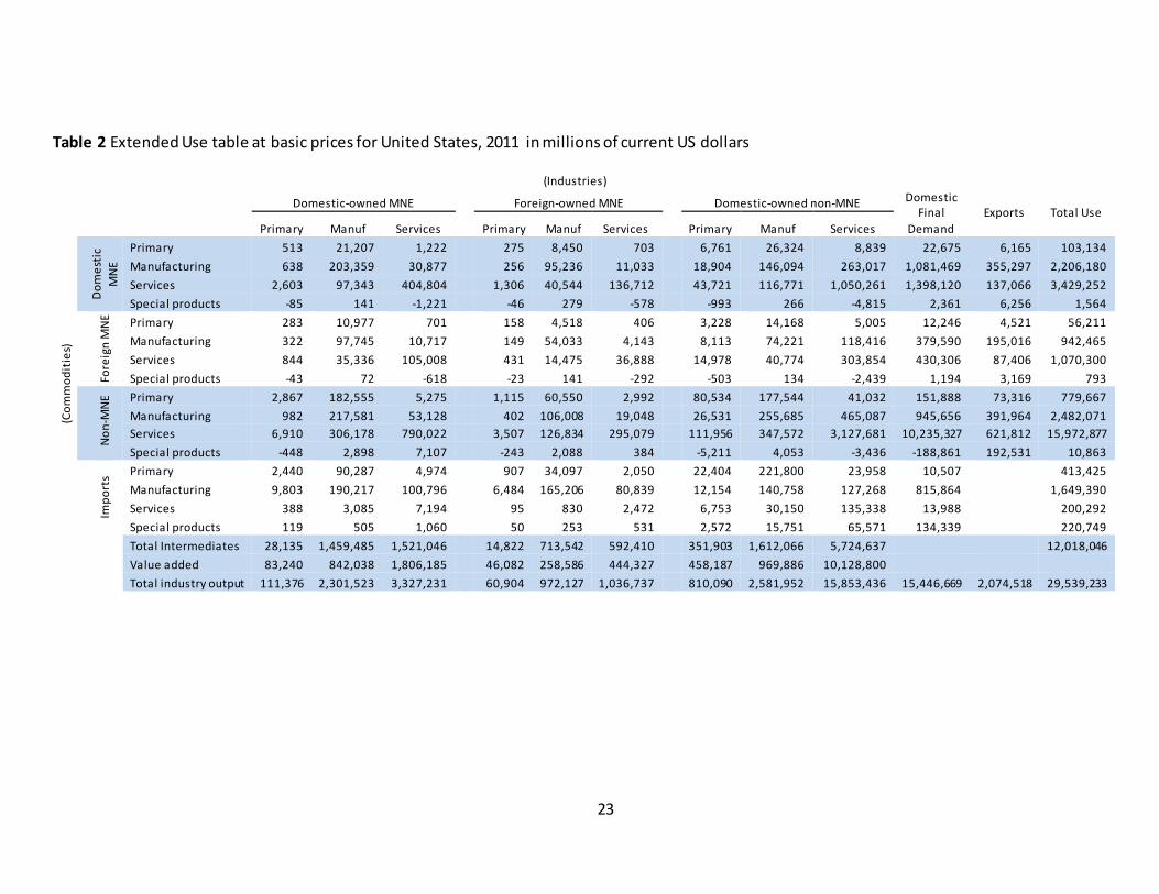
Tables 1 and 2 show a highly aggregated example of our proof-of-concept, extended

SUTs for the United States for 2011. Across the columns, the supply and use tables are arranged

first by the three firm-types: domestic-owned MNEs, foreign-owned MNEs, and domestic-

owned non-MNEs. The columns show an aggregation of industries of primary goods,

manufacturing, services, and unclassified “special” products. In this aggregation, the primary

11

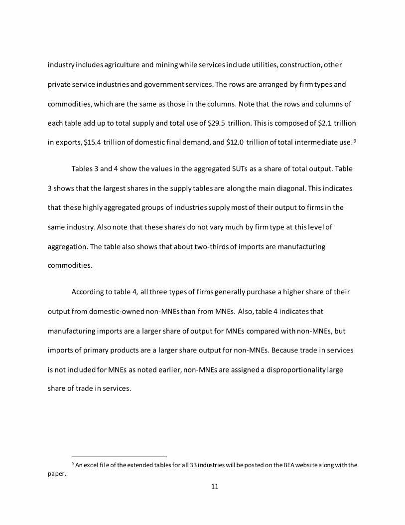
industry includes agriculture and mining while services include utilities, construction, other

private service industries and government services. The rows are arranged by firm types and

commodities, which are the same as those in the columns. Note that the rows and columns of

each table add up to total supply and total use of $29.5 trillion. This is composed of $2.1 trillion

in exports, $15.4 trillion of domestic final demand, and $12.0 trillion of total intermediate use.9

Tables 3 and 4 show the values in the aggregated SUTs as a share of total output. Table

3 shows that the largest shares in the supply tables are along the main diagonal. This indicates

that these highly aggregated groups of industries supply most of their output to firms in the

same industry. Also note that these shares do not vary much by firm type at this level of

aggregation. The table also shows that about two-thirds of imports are manufacturing

commodities.

According to table 4, all three types of firms generally purchase a higher share of their

output from domestic-owned non-MNEs than from MNEs. Also, table 4 indicates that

manufacturing imports are a larger share of output for MNEs compared with non-MNEs, but

imports of primary products are a larger share output for non-MNEs. Because trade in services

is not included for MNEs as noted earlier, non-MNEs are assigned a disproportionality large

share of trade in services.

9 An excel fi le of the extended tables for all 33 industries will be posted on the BEA website along with the

paper.

12

4.2 TiVA estimates

Once the extended SUTs are constructed, we derive a symmetric industry-by-industry

extended IOT from the extended SUTs. First, we generate a commodity-by-commodity IOT

using the industry technology assumption that each industry has its own specific method of

production, irrespective of its product mix. We derive an industry-by-industry IOT using the

fixed product sales structure approach from this table, in which each product has its own

specific sales structure, irrespective of the industry in which it is produced.10 Dietzenbacher, Los,

Stehrer, Timmer, and de Vries (2013) note that this approach is also used to construct the world

IOTs for the World Input-Output Database Project. They indicate that practitioners prefer the

fixed product sales structure approach to the fixed industry sales structure where each industry

has its own sales structure. This is because it is more plausible that products have the same

sales structure than industries having the same sales structure. It also does not yield negative

values in cells that were not negative in the original SUT.

TiVA estimates are most rigorously calculated using international IOTs that account for

the production of all countries in the world. However, TiVA statistics can be calculated using

single country IOTs. We follow the approach of Ma, Wang, and Zhu (2015) and Tang, Wang, and

Wang (2014) and assume that domestic content in gross exports is the same as the value added

in exports. Because part of domestic content in gross exports is re-imported goods, domestic

content is an upper bound on domestic value added.

10 Eurostat (2008).

13

We calculate TiVA measures using a methodology that is typically used for international

IOTs. A key to calculating TiVA statistics is the Leontief inverse of the IOT. The matrix depends

on both the direct input requirements from the same industry and the indirect input

requirements from other industries. Domestic value added embodied in gross exports for a

particular industry depends on both these direct and indirect requirements. Following Ma,

Wang, and Zhu (2015) and Tang, Wang, and Wang (2014), we calculate domestic value added as

the product of the vector of the domestic value added share of output for each industry, the

Leontief inverse of the U.S. IOT matrix, and the value of gross exports for each industry.

Likewise, the direct domestic value added content of gross exports is calculated as the vector of

domestic value added shares of output multiplied by the value of gross exports for each

industry. Indirect domestic content of gross exports is calculated as the difference between

total and direct domestic value added.

5 Results

In this section we describe the TiVA indicators from the U.S. IOTs. These TiVA indicators

help us better understand how an economy engages in global value chains. We find that the

domestic value added of exports is similar across large industry groups. However, there is much

more variation in the value added share of exports once firm type is considered. Also, the share

of this value added that comes directly from the producing industry varies much more across

industries than within industries.

14

Powers (2012) points out that TiVA indicators typically focus on either a decomposition

of value added where goods are consumed or a decomposition of gross trade. He indicates that

examining trade on a value added basis shows a different picture of bilateral trade balances

than gross trade flows. However, the total trade deficit summed across all countries is identical

for both TiVA and gross trade flows.

One core measure of TiVA is decomposing value added of gross exports and imports into

domestic and foreign components. Other things being equal, the higher the foreign value added

share of exports, the more a particular industry is integrated in global value chains. This could

mean that the current level of exports depends on foreign content. It is also possible that the

foreign content is substituted for potential additional domestic content.

According to the OECD TiVA database, domestic value added as a share of exports for

the United States fluctuated slightly between 85 and 89 percent between 1997 and 2013. The

share is stable around 89 percent during 1997 to 2002 and then gradually decreases to 85

percent in 2008. Domestic value added embodied in gross exports fluctuates between 86 and

89 percent of gross exports during 2009 to 2013. The fluctuations during this period are most

likely due to the contraction of international trade following the financial crisis and the

subsequent recovery during that period.11

Domestic value added is a relatively larger share of exports for the United States

compared with other major economies. Domestic value added as a share of exports in 2011 for

the United States is similar to the share of domestic value added in exports for Australia, Japan, 11 OECD Trade in Value Added Database, Updated October 2015.

15

and Russia, but about 10 percentage points higher than the share for most major European

countries and Canada, about 17 percentage points higher than the share for China and Mexico,

and about 27 percentage points higher than the share of domestic valued in exports for Korea.12

While this seems to suggest that the United States is relatively less integrated into global value

chains than many other major economies, it has the third highest level of foreign value added

content in exports in the world in 2011 at $286 billion. The only other countries with greater

foreign value added content of gross exports were China at $632 billion and Germany at $365

billion.

Before estimating TiVA statistics by firm type from the extended U.S. IOT, we calculate

TiVA statistics for all U.S. firms based on the 71 industry 2011 U.S. make and use tables.

Domestic value added as a share of gross exports for the United States varies by industry in

2011. As seen in figure 1, industries in the service sector generally have the highest shares of

domestic value added in their exports. Domestic value added as a share of exports for

industries in the services sector ranges from 77 percent to 99 percent. This is not surprising

given the labor intensive nature of services. One exception is the relatively more capital

intensive transportation services for which domestic value added as a share of exports is about

78 percent to 86 percent. Domestic value added as a share of output is slightly smaller for the

mining and extraction sector for which many inputs are geographically constrained to have a

domestic location compared to the services sector. Figure 2 shows that industries in the

manufacturing sector have more heterogeneity in the domestic value added as share of output,

12 “Domestic value added share of gross exports,” October 2015, OECD TiVA database.

16

but in most cases the share is between 81 and 87 percent. A notable exception is petroleum and

coal products for which domestic value added makes up only slightly more than one half of the

value of exports. In 2011, the industry most likely used more imported foreign crude oil and

coal to produce refined petroleum and coal products for export.

Another core TiVA measure is to decompose the share of domestic value added in gross

exports into value added directly in the industry and indirect value added from other domestic

industries. This decomposition measures the degree to which an industry participates in a

domestic supply chain. Focusing on manufacturing industries in 2011, we see from figure 3 that

both direct and indirect domestic value added as a share of gross exports vary much more by

manufacturing industry than domestic value added as a share of gross exports.

The computer and electronic products industry has the largest share of direct domestic

value added in its gross exports. This reflects the industry’s high investment in R&D and its high-

skilled, high-paid labor force. The food, beverage, and tobacco industry has the largest share of

indirect domestic value added in its gross exports. This reflects the fact that its domestic value

added content mainly comes through intermediate inputs, particularly agricultural inputs.

Next we estimate TiVA statistics by firm type from our extended IOTs. Domestic value

added as share of exports does not vary much by type of firm on average, but the difference

varies between different types of firms for a particular industry. Table 5 shows that domestic

value added makes up 86 percent of gross exports for domestic-owned MNEs in 2011, similar to

the 88 percent share for non-MNEs, and the 80 percent share for foreign-owned MNEs.

17

However, this share varies widely by industry, ranging from a minimum of 62 percent for coke,

petroleum products, and nuclear fuel to a maximum of 98 percent for renting of machinery and

equipment.

Table 6 shows that there are many instances of variability in domestic value added as a

share of output across different types of firms in the same industry. Domestic value added as a

share of output is smaller for foreign-owned MNEs compared with both domestic-owned MNEs

and domestic non-MNEs for all but a few industries. Although there are sizable differences

between domestic value added as a share of output for domestic-owned MNEs and non-MNEs

for many industries, there is no clear pattern for direction of those differences. The largest

differences are in agriculture and textiles.

Table 7 shows that although the average direct and indirect value added embodied in

gross exports is similar across firm type, there are differences by industry. The largest

differences are between MNEs and non-MNEs. For example, in the food products, beverage,

and tobacco industry, direct domestic value makes up more than 72 percent of the value of

gross exports while indirect domestic value makes up 69 percent of the value of gross exports

for non-MNEs. This suggests that the non-MNEs are much more integrated in domestic value

chains (including vertically integrated single firms) in these industries.

6 Conclusion

In this paper we construct proof-of-concept extended SUTs and TiVA estimates for the

United States. We do so by disaggregating production characteristics by type of firm and

18

applying them to recently-introduced SUTs for the United States by the BEA (Young, Howells III,

Strassner and Wasshausen 2015). The project requires some modeling of basic price valuations

in order to translate BEA’s official use tables into domestic and import use, and to refine the

valuation of intermediate inputs and final demand from purchaser price valuation to basic

prices. This refinement to basic prices can be important for better understanding the economic

activity based on the theory of the firm. Basic price valuation removes taxation and trade policy

distortion from the estimates.

The results from this work build on a body of evidence found in other studies about the

importance of reflecting firm-level heterogeneity in traditional SUTs to understand global value

chains better through TiVA analysis. Our results indicate that heterogeneity by firm-type and by

ownership does matter particularly for industries such as agriculture, textiles, and construction.

Our analysis also reveals that it is a useful exercise to estimate TiVA from a single country SUT

and IOT. For example, the single-model approach does indeed allow for distinctions to be made

about how engaged domestic industries are in both global and domestic value chains, even if

there are some limitations in interpreting the indirect value added estimates. For example,

direct and indirect value added estimates reveal that the degree to which firms are integrated

in domestic production chains varies widely by industry.

Looking ahead, there are a suite of projects that remain on the agenda for the BEA and

for the USITC. These include collaborations with the OECD and with the Asia-Pacific Economic

Cooperation (APEC) where work continues to develop the framework for extended SUTs and to

develop APEC region SUTs and IOTs and associated TiVA estimates. The aim of this work is to

19

incorporate the APEC database into the OECD database sometime around 2018. Additionally,

the BEA and the USITC are collaborating with Statistics Canada and the Instituto Nacional de

Estadistíca y Geografía to develop North America Regional SUTs and TiVA statistics with a goal

to complete the regional SUT and TiVA statistics in 2018 and extended tables and TiVA

measures around 2020.

Lastly, much work remains at the BEA to improve the economic infrastructure to

support global value chain efforts. This work includes enhancing the international comparability

of BEA’s SUTs and expanding the detail BEA publishes by type of service and by country. In

addition, a critical element is to produce official extended SUTs after completing a five-year

microdata linking project with the Census Bureau. This project will link BEA’s AMNE and trade in

services data with data from Census Bureau economic censuses and establishment surveys and

data on trade in goods. The output of this linking project will identify firm-level heterogeneity

tabulations that, ideally, will be made available for use on a recurring basis to construct official

statistics.

20

Bibliography

Ahmad, N., Araujo, S., Lo Turco, A., & Maggioni, D. (2013). Using trade microdata to improve trade in value added measures: proof of concept using Turkish data. Mattoo, A., Wang, Z. and Wei, S. (Eds.), Trade in Valued Added: Developing New Measures of Cross-Border Trade (pp. 187-219.) Washington, DC: The World Bank.

Barefoot, K. & Koncz-Bruner, J. (2012). A profile of U.S. exporters and importers of services. Survey of Current Business, 92(6), 66-87.

Bernard, A. B., Jensen, J. B., & Schott, P.K. (2009). Importers, exporters, and multinationals. In Dunne, T., Jensen J. B., and Roberts, M. J. (Eds.), Producer dynamics: new evidence from micro data (pp. 513-551). Cambridge, MA: NBER, University of Chicago Press.

Curcuru, S. E. & Thomas, C. P. (2015). The return on U.S. direct investment at home and abroad. In Hulten, C. R. and Reinsdorf, M. B. (Eds.), Measuring wealth and financial intermediation and their links to the real economy (pp. 205-230). Cambridge, MA: NBER, University of Chicago Press. Dietzenbacher ,E., Los, B., Stehrer, R., Timmer, M.P., and de Vries, G.J. (2013). The Construction of World Input-Output Tables in the WIOD Project. Economic Systems Research, 25, 71-98. Fetzer, J.J. & Strassner, E.H. (2015). Identifying Heterogeneity in the Production Components of Globally Engaged Business Enterprises in the United States, BEA Working Paper WP2015-13. Johnson, Robert C. & Noguera, Guillermo (2012). Accounting for intermediates: production sharing and trade in value added. Journal of International Economics, 86(2), 224-236. Koopman, Wang, and Wei (2012). Tracing value-added and double counting in gross exports. American Economic Review, 104(2), 459-494. Los, B., Timmer, M.P. & de Vries, G.J. (Forthcoming). Tracing value-added and double counting in gross exports: comment. American Economic Review. Ma, H., Wang, Z., & Zhu, K. (2015). Domestic content in China’s exports and its distribution by firm ownership. Journal of Comparative Economics, 43(1), 3-18. Piacentini, M. & Fortanier, F. (2015). Firm heterogeneity and trade in value added. OECD Working Paper.

Samuels, J. D., Howells III, T. F., Russell, M., & Strassner, E. H. (2015). Import allocations across industries, import prices across countries, and estimates of industry growth and productivity. Houseman, S. N., & Mandel, M., (Eds.), Measuring globalization: better trade statistics for better policy (pp. 251-289.). Kalamazoo, MI: W.E. Upjohn Institute for Employment Research.

21

Tang, H., Wang, F., & Wang Z. (2014). The Domestic Segment of Global Supply Chains in China Under State Capitalism. World Bank Policy Research Paper 6960.

Young, J. A., Howells III, T. F., Strassner, E.H., & Wasshausen, D.B. (2015). BEA Briefing: Supply-Use Tables for the United States. Survey of Current Business 95:(9) , 1-8.

22

Table 1 Extended supply table at basic prices for United States, 2011 in millions of current US dollars

(Industries)

Domestic-owned MNE

Foreign-owned MNE

Domestic-owned non-MNE Imports Commodity

Supply

Primary Manuf Services

Primary Manuf Services

Primary Manuf Services

(Com

mod

ities

)

Dom

estic

M

NE Primary 102,770 177 186 103,134

Manufacturing 5,590 2,193,731 6,859 2,206,180 Services 3,015 106,170 3,320,068 3,429,252 Special products 0 1,446 119 1,564

Fore

ign

MNE

Primary

55,927 180 104

56,211 Manufacturing

3,246 936,219 3,000

942,465

Services

1,731 34,961 1,033,608

1,070,300 Special products

0 767 25

793

Non

-MNE

Primary 774,138 324 5,205 779,667 Manufacturing 22,072 2,430,895 29,104 2,482,071 Services 13,880 148,278 15,810,718 15,972,877 Special products 0 2,455 8,408 10,863

Impo

rts Primary

413,425 413,425

Manufacturing

1,649,390 1,649,390 Services

200,292 200,292

Special products

220,749 220,749

Total industry output 111,376 2,301,523 3,327,231 60,904 972,127 1,036,737 810,090 2,581,952 15,853,436 2,483,856 29,539,233

23

Table 2 Extended Use table at basic prices for United States, 2011 in millions of current US dollars

(Industries)

Domestic-owned MNE

Foreign-owned MNE

Domestic-owned non-MNE Domestic

Final Demand

Exports Total Use

Primary Manuf Services

Primary Manuf Services

Primary Manuf Services

(Com

mod

itie

s)

Dom

esti

c M

NE

Primary 513 21,207 1,222 275 8,450 703 6,761 26,324 8,839 22,675 6,165 103,134 Manufacturing 638 203,359 30,877 256 95,236 11,033 18,904 146,094 263,017 1,081,469 355,297 2,206,180 Services 2,603 97,343 404,804 1,306 40,544 136,712 43,721 116,771 1,050,261 1,398,120 137,066 3,429,252 Special products -85 141 -1,221 -46 279 -578 -993 266 -4,815 2,361 6,256 1,564

Fore

ign

MN

E Primary 283 10,977 701

158 4,518 406

3,228 14,168 5,005 12,246 4,521 56,211 Manufacturing 322 97,745 10,717

149 54,033 4,143

8,113 74,221 118,416 379,590 195,016 942,465

Services 844 35,336 105,008

431 14,475 36,888

14,978 40,774 303,854 430,306 87,406 1,070,300 Special products -43 72 -618

-23 141 -292

-503 134 -2,439 1,194 3,169 793

Non

-MN

E Primary 2,867 182,555 5,275 1,115 60,550 2,992 80,534 177,544 41,032 151,888 73,316 779,667 Manufacturing 982 217,581 53,128 402 106,008 19,048 26,531 255,685 465,087 945,656 391,964 2,482,071 Services 6,910 306,178 790,022 3,507 126,834 295,079 111,956 347,572 3,127,681 10,235,327 621,812 15,972,877 Special products -448 2,898 7,107 -243 2,088 384 -5,211 4,053 -3,436 -188,861 192,531 10,863

Impo

rts Primary 2,440 90,287 4,974

907 34,097 2,050

22,404 221,800 23,958 10,507

413,425

Manufacturing 9,803 190,217 100,796

6,484 165,206 80,839

12,154 140,758 127,268 815,864

1,649,390 Services 388 3,085 7,194

95 830 2,472

6,753 30,150 135,338 13,988

200,292

Special products 119 505 1,060

50 253 531

2,572 15,751 65,571 134,339

220,749

Total Intermediates 28,135 1,459,485 1,521,046 14,822 713,542 592,410 351,903 1,612,066 5,724,637 12,018,046

Value added 83,240 842,038 1,806,185 46,082 258,586 444,327 458,187 969,886 10,128,800

Total industry output 111,376 2,301,523 3,327,231 60,904 972,127 1,036,737 810,090 2,581,952 15,853,436 15,446,669 2,074,518 29,539,233

24

Table 3 Extended supply table at basic prices for United States, 2011, share of total output

(Industries)

Domestic-owned MNE

Foreign-owned MNE

Domestic-owned non-MNE Imports Commodity

Supply

Primary Manuf Services

Primary Manuf Services

Primary Manuf Services

(Com

mod

ities

)

Dom

estic

M

NE Primary 92 0 0 0

Manufacturing 5 95 0 7 Services 3 5 100 12 Special products 0 0 0 0

Fore

ign

MNE

Primary

92 0 0

0 Manufacturing

5 96 0

3

Services

3 4 100

4 Special products

0 0 0

0

Non

-MNE

Primary 96 0 0 3 Manufacturing 3 94 0 8 Services 2 6 100 54 Special products 0 0 0 0

Impo

rts Primary

17 1

Manufacturing

66 6 Services

8 1

Special products

9 1

Total industry output 100 100 100 100 100 100 100 100 100 100 100

25

Table 4 Extended use table at basic prices for United States, 2011, share of total output

(Industries)

Domestic-owned MNE

Foreign-owned MNE

Domestic-owned non-MNE Domestic Final

Demand Exports Total Use

Primary Manuf Services

Primary Manuf Services

Primary Manuf Services

(Com

mod

ities

)

Dom

estic

M

NE Primary 0 1 0 0 1 0 1 1 0 0 0 0

Manufacturing 1 9 1 0 10 1 2 6 2 7 17 7 Services 2 4 12 2 4 13 5 5 7 9 7 12 Special products 0 0 0 0 0 0 0 0 0 0 0 0

Fore

ign

MNE

Primary 0 0 0

0 0 0

0 1 0 0 0 0 Manufacturing 0 4 0

0 6 0

1 3 1 2 9 3

Services 1 2 3

1 1 4

2 2 2 3 4 4 Special products 0 0 0

0 0 0

0 0 0 0 0 0

Non

-MNE

Primary 3 8 0 2 6 0 10 7 0 1 4 3 Manufacturing 1 9 2 1 11 2 3 10 3 6 19 8 Services 6 13 24 6 13 28 14 13 20 66 30 54 Special products 0 0 0 0 0 0 -1 0 0 -1 9 0

Impo

rts Primary 2 4 0

1 4 0

3 9 0 0

1

Manufacturing 9 8 3

11 17 8

2 5 1 5

6 Services 0 0 0

0 0 0

1 1 1 0

1

Special products 0 0 0

0 0 0

0 1 0 1

1

Total Intermediates 25 63 46 24 73 57 43 62 36 41

Value added 75 37 54 76 27 43 57 38 64

Total industry output 100 100 100 100 100 100 100 100 100 100 100 100

26

Table 5 Domestic value added as a share of exports, by type of firm, by industry, 2011

ISIC Description Domestic

MNE Foreign

MNE Non-MNE

I01 Agriculture, hunting, forestry, and fishing 64 40 91 I02 Mining and quarrying 93 91 94 I03 Food products, beverages, and tobacco 92 89 86 I04 Textiles, textile products, leather, and footwear 76 58 90 I05 Wood and products of wood and cork 83 75 89 I06 Pulp, paper, paper products, printing, and publishing 91 78 93 I07 Coke refined petroleum products and nuclear fuel 62 57 47 I08 Chemicals and chemical products 90 87 92 I09 Rubber and plastics products 85 83 83 I10 Other non-metallic mineral products 85 90 86 I11 Basic metals 83 78 70 I12 Fabricated metal products except machinery and equip. 81 77 85 I13 Machinery and equipment n.e.c 83 77 81 I14 Computer electronic and optical products 93 82 91 I15 Electrical machinery and apparatus n.e.c 82 72 81 I16 Motor vehicles trailers and semi-trailers 81 76 73 I17 Other transport equipment 84 74 84 I18 Manufacturing n.e.c; recycling 92 83 80 I19 Electricity, gas, and water supply 93 88 93 I20 Construction 88 68 90 I21 Wholesale and retail trade; repairs 96 94 96 I22 Hotels and restaurants 93 89 94 I23 Transport and storage 91 83 81 I24 Post and telecommunications 93 87 91 I25 Finance and insurance 96 96 92 I26 Real estate activities 94 94 98 I27 Renting of machinery and equipment 97 88 95 I28 Computer and related activities 95 87 95 I29 Other business activities (incl. R&D) 95 90 96 I30 Public admin. and defence; compulsory social security 94 I31 Education 93 83 96 I32 Health and social work 88 69 96 I33 Other community, social, and personal services 91 78 95 All Industries 86 80 88 Minimum 62 40 47 Maximum 97 96 98

Note: The darker blue a cell is, the greater its value is from the “grand median” of all values in the table of 88. The darker red a cell is, the lesser its value is compared with 88.

27

Table 6 Differences in domestic value added as a share of exports, by type of firm, by industry, 2011

ISIC Description

Foreign MNE minus

Domestic MNE

Foreign MNE minus Non-MNE

Domestic MNE minus

Non-MNE

I01 Agriculture, hunting, forestry, and fishing -24 -51 -27 I02 Mining and quarrying -1 -2 -1 I03 Food products, beverages, and tobacco -2 4 6 I04 Textiles, textile products, leather, and footwear -18 -32 -14 I05 Wood and products of wood and cork -8 -13 -6 I06 Pulp, paper, paper products, printing, and publishing -14 -15 -2 I07 Coke refined petroleum products and nuclear fuel -5 10 15 I08 Chemicals and chemical products -3 -5 -2 I09 Rubber and plastics products -3 0 3 I10 Other non-metallic mineral products 5 4 -1 I11 Basic metals -4 8 13 I12 Fabricated metal products except machinery and equip. -4 -8 -3 I13 Machinery and equipment n.e.c -5 -4 2 I14 Computer electronic and optical products -11 -9 2 I15 Electrical machinery and apparatus n.e.c -9 -8 1 I16 Motor vehicles trailers and semi-trailers -5 3 8 I17 Other transport equipment -11 -11 0 I18 Manufacturing n.e.c; recycling -9 3 12 I19 Electricity, gas, and water supply -5 -5 0 I20 Construction -20 -22 -2 I21 Wholesale and retail trade; repairs -3 -3 0 I22 Hotels and restaurants -4 -5 -1 I23 Transport and storage -8 2 10 I24 Post and telecommunications -6 -4 2 I25 Finance and insurance 0 3 4 I26 Real estate activities 1 -4 -5 I27 Renting of machinery and equipment -8 -7 1 I28 Computer and related activities -8 -8 0 I29 Other business activities (incl. R&D) -5 -5 -1 I30 Public admin. and defence; compulsory social security

I31 Education -10 -13 -3 I32 Health and social work -19 -27 -9 I33 Other community, social, and personal services -12 -17 -4

Note: Blue cells indicate negative values and yellow cells indicate positive values.

28

Table 7 Direct and indirect domestic value added as a share of gross output, by type of firm, by industry, 2011

ISIC Description Direct Indirect Dom. MNE

For. MNE

Non- MNE

Dom. MNE

For. MNE

Non- MNE

I01 Agriculture, hunting, forestry, and fishing 15 19 54 49 21 37 I02 Mining and quarrying 30 36 17 62 56 77 I03 Food products, beverages, and tobacco 78 72 16 13 17 69 I04 Textiles, textile products, leather, and footwear 51 33 69 25 25 20 I05 Wood and products of wood and cork 21 35 36 63 40 53 I06 Pulp, paper, paper products, printing, and publishing 42 40 68 50 37 25 I07 Coke refined petroleum products and nuclear fuel 46 48 21 16 9 26 I08 Chemicals and chemical products 61 58 48 29 29 44 I09 Rubber and plastics products 28 42 53 57 40 30 I10 Other non-metallic mineral products 51 36 53 34 54 33 I11 Basic metals 28 24 23 54 54 47 I12 Fabricated metal products except machinery and

equipment 34 35 35 48 42 50

I13 Machinery and equipment n.e.c 74 67 73 9 11 8 I14 Computer electronic and optical products 80 76 70 13 7 21 I15 Electrical machinery and apparatus n.e.c 74 66 52 8 6 29 I16 Motor vehicles trailers and semi-trailers 42 59 70 39 17 3 I17 Other transport equipment 59 67 84 25 7 1 I18 Manufacturing n.e.c; recycling 88 81 78 4 2 2 I19 Electricity, gas, and water supply 18 6 2 74 82 91 I20 Construction 32 5 0 56 63 90 I21 Wholesale and retail trade; repairs 42 54 16 55 39 80 I22 Hotels and restaurants 14 6 16 79 83 78 I23 Transport and storage 1 3 58 91 80 23 I24 Post and telecommunications 27 25 41 66 63 50 I25 Finance and insurance 1 0 71 95 95 22 I26 Real estate activities 0 0 7 93 94 91 I27 Renting of machinery and equipment 6 3 70 91 85 25 I28 Computer and related activities 58 14 44 37 73 52 I29 Other business activities (incl. R&D) 4 3 16 91 87 80 I30 Public admin. and defence; compulsory social security 0 0 85 0 0 9 I31 Education 37 20 51 56 62 45 I32 Health and social work 27 63 52 60 7 45 I33 Other community, social, and personal services 26 29 59 64 50 36 All Industries 47 47 49 39 33 39 Note: The darker blue a cell is, the greater its value is from the “grand median” of all values in the table of 38. The darker red a cell is, the lesser its value compared with 38.

29

Figure 1 Domestic value added as a share of gross exports by industry, 2011

0

20

40

60

80

100

Shar

e of

gros

s exp

orts

Transportation Services

Services Manufacturing Mining/ Extraction

All industry average share= 86 percent

Farms/ Forestry/ Fishing

Utilities/ Construction

30

Figure 2 Domestic value added as a share of gross exports by manufacturing industry, 2011

87 88

72

83 79

8980

7181 82

87 85 8187

8188

54

8580

0

20

40

60

80

100

Shar

e of

gros

s exp

orts

31

Figure 3 Direct and indirect domestic value added (DVA) as a share of gross exports by manufacturing industry, 2011

31 3820

38 36

64

3922

44 3648

25 2839

3046

2141

32

56 50

52

45 44

25

40

49

37 4639

60 5348

51

42

33

4448

0

20

40

60

80

100

Shar

e of

gros

s exp

orts

Direct DVA Indirect DVA

32

Appendix A: Refining the use table valued at basic prices

To develop separate matrices for domestically-produced inputs valued at basic prices,

imported inputs at basic prices, margins, taxes on products, and subsidies on products, we solve

a quadratic programming model with parameters from BEA’s published SUTs. Before

introducing the estimation model, let us review the major data reported in the BEA Supply-Use

IO tables. At the product and sector level (73 groups of products and 71 industries), we know

the following values from the supply table:

cjtx0 = Output of product group c by industry j at year t, basic prices, 73 by 71 matrix;

ctm0 = Imports from the world of product group c at year t, cif prices, 73 by 1 vector;

ctTSb0 = Total supply of product c at year t, basic prices;

ctTmg0 = Total trade margins by product c at year t, 73 by 1 vector;

ctTtrs0 = Total transport margins by product c at year t, 73 by 1 vector; itxctTtxc0 = Total tax by product c at year t, (import duty, Tax and Subsidies) 73 by 3

matrix

ctTSp0 = Total supply of product c at year t, purchaser prices, 71 by 1 vector; We also know following values from the use tables:

citzp0 = Product c used by industry i at year t, purchaser prices, 73 by 71 matrix

itvb0 = total value added of industry i at basic prices at year t, 1 by 71 vector

itTXIb0 = Total output of industry i at year t, basic prices, 1 by 71 vector itxitTtxi0 = Total tax/duty or subsidy by industry i at year t, (tax and import duties,

subsidies 2 by 71 matrix)

chtyp0 = Product c used by final user h at year t, purchaser prices

cte0 = Exports to the world of product group c at year t, fob prices

ctTUp0 = Total use of product group c at year t, purchaser prices; From the import use tables we know these values:

citzmb0 = Imported product c used by industry i at year t, basic prices

33

chtymb0 = Imported product c used by final user h at year t, basic prices These data will be used as parameters (right hand constant) to construct the linear

constraints and the initial value of variables in the estimation model.

Model specification: The notation used to specify the programming model is as follows: Index: I ={ 01…71}; C ={ 01…73}; H = { F01,F02,IVT ,GOV, EXP} NMG ={ 1…26,36,38…73}; MGC ={ 27…35,37};ITX={TAX,DUTY,SUB} Variables (Unknowns: basic-price-based intermediate transactions and final demand

transactions) :

citzb = Product c used by industry i at year t, basic prices

chtyb = Product c used by final user h at year t, basic prices

citzdb = Domestic made product c used by industry i at year t, basic prices

chtydb = Domestic made product c used by final user h at year t, basic prices The following variables constitute the valuation matrix. Each margin has the same

dimension as the corresponding use table: mgccitmgi = Trade and transport margins for intermediate input of Product c used by

industry i at year t (10 by 73 by 71 array); mgccitmgy = Trade and transport margins for final use of Product c used by final user h at

year t (10 by 73 by 5 array) itxcitntxi = tax for intermediate input of Product c used by industry i at year t (3 by 73 by

71 array); itxchtntxy = tax for final use of Product c used by final user h at year t (3 by 73 by 71 array);

The estimation model is based on the economic and statistical relationship between

elements in the use table valued at basic prices and elements in the use table valued at

purchaser prices. These are used to construct several linear equations as constraints and to

compute the initial values of variables that are used to formulate an optimization problem to

minimize the deviation of the solution values from the initial values of these variables.

34

Constraints: The relationship between cells of the use table based on basic prices and the use table

based on purchaser prices is:

For non-margin products: C = NMG

cititx

itx

mgc

mgccitcit zpnetimgizb

cit0

3

1

10

1=++ ∑∑

==

(A.1)

chtitx

itx

mgc

mgcchtcht ypntxymgyyb

cht0

3

1

10

1=++ ∑∑

==

(A.2)

For margin products: C=MGC

cititx

itx

nmg

mgccitcit zpnetimgizb

cit0

3

1

73

=+− ∑∑=

(A.3)

chtitx

itx

nmg

mgcchtcht ypntxymgyyb

cht0

3

1

73

=+− ∑∑=

(A.4)

The split between domestic and import use at basic prices is assumed to be:

citcitcit zbzmzd =+ 0 (A.5)

chtchtcht ybymyd =+ 0 (A.6) Basic balance condition Supply and use balance for each product groups at purchaser prices: For non-margin products: C=NMG

cth itx

itx

mgc

mgcchtcht

i itx

itx

mgc

mgccitcit TSpntxymgyybnetimgizb

chtcit0)()(

5

1

3

1

10

1

71

1

3

1

10

1=+++++ ∑ ∑∑∑ ∑∑

= === ==

(A.7)

For margin products: C=MGC

cth itx

itx

nmg

mgcchtcht

i itx

itx

nmg

mgccitcit TSpntxymgyybnetimgizb

chtcit0)()(

5

1

3

1

7371

1

3

1

73

=+−++− ∑ ∑∑∑ ∑∑= == =

(A.8)

Supply and use balance for each product group at basic prices:

35

0 0071

1

5

1

71

1ct

ictcit

hcht

subtax

icit TSbmxybnetinetizb

citcit=+=+++ ∑∑∑

===

for all c (A.9)

Input cost and total output balance for each industry at basic prices:

itc

ictl

iftsubtax

citcit1=c

TXIbxvbnetinetizmzd citcit

000)0(73

1

3

1

73

∑∑∑==

==++++ for all i (A.10)

Balance condition for total domestic product output and use at basic prices:

∑∑∑=

=+++71

1

671

0i

ictsubtax

cht=1h

cit=1i

xnetinetiydzd citcit

for all c (A.11)

Balance condition for total import supply and use at basic prices:

ctcht=1h

cit=1i

mymzm 0771

=+∑∑ for all c (A.12)

Transportation cost, trade margins and net tax constraints Trade and transport margin supply and use balance: For MGC={27…31}

ctnmgc i

mgccht

mgccit Tmgmgymgi 0)(

73 71

1−=+∑ ∑

= =

(A.13)

For MGC ={32…35,37}

ctnmgc i

mgccht

mgccit Ttrsmgymgi 0)(

73 71

1−=+∑ ∑

= =

(A.14)

Domestic trade and transportation cost constraints for non-margin products: For C=NMG and MGC={27…31}

ctmgc h

mgccht

mgc i

mgccit Tmgmgymgi 0

5

1

71

1=+∑∑∑∑

==

(A.15)

For C=NMG and MGC={32…35,37}

ctmgc h

mgccht

mgc i

mgccit Ttrsmgymgi 0

5

1

71

1=+∑∑∑∑

==

(A.16)

Tax constraints for each product group:

itxct

h

itxcht

i

itx Ttxcntxyntxicit

05

1

71

1=+∑∑

==

for all c (A.17)

Tax and duty constraints for each industry:

36

itxit

c

itx Ttxintxicit

073

1=∑

=

for all i (A.18)

Aggregate expenditure components constraints:

htitx

itxcht

nmg mgc

mgccht

hcht

c

GDPEntxymgyyb =++ ∑∑ ∑∑∑===

)(3

1

73 10

1

473

1 for all h except EXP (A.19)

GDP from the production side:

ti c itx

itxcit

fift GDPntxivb∑ ∑∑∑

= = ==

=+71

1

73

1

3

1

3

1) (A.20)

GDP from the expenditure side:

tc

ctcth

ht GDPmeGDPE =−+∑∑==

])00(73

1

5

1 (A.21)

The objective function:

−

++

+++

+−

+−

∑∑∑∑∑∑

∑∑∑∑ ∑∑∑∑

∑∑∑∑∑∑

== =

−

=

−

== = =

−

=

−

=

−

= == =

ntxi

ntxintxi ntxy

ntxyntxy

mgy

mgymgy

mgimgimgi

ymymym

ydydyd

zmzmzm

zdzdzd

citxcit

itxcit

itxcit

1=itx1=ih itxitxcht

itxcht

itxcht

=c

h

mgccht

mgccht

mgccht

c=mgcmgc i cmgccit

mgccit

mgccit

h cht

chtcht

=c

h cht

chtcht

=cc i cit

citcit

c i cit

citcit

73

1

23716

1

3

1

2(

73

1

6

1

2(

73

1

10

1

10

1

71

1

73

1

2(6

1

2(

73

1

6

1

2(

71

1

73

1

71

1

273

1

71

1

2

0)0(

0)0

0)0

0)0

0)0

0)0)0(

0)0(

21= SMin

To obtain a solution the problem, we minimize the objective function subject to

constraints (A.1) to (A.21).

Initial values for all unknowns in the constrained optimization problem are based on

various proportionality assumptions and other BEA data. Notice that the initial values obtained

usually do not satisfy the linear constraints.

Variable initiation:

ct

itxctitx

ct TSbTtxc

=τ (tax rate computed from supply table)

37

itxcitntxi0 = itx

ctτ citprz _ net tax rate multiplied by industry cells at producer prices from the traditional use table;

itxchtntxy0 = cht

itxct pry _τ net tax rate multiplied by final demand by categories at

producer prices from the traditional use tables

citzmb0 = industry cells from the import use table before redefinition

chtymb0 = final demand by categories from the import use table before redefinition

citzdb0 = ∑=

−−3

100_

itxcitcitcit ntxizmbprz

chtydb0 = ∑=

−−3

100_

itxchtcitcit ntxyymbpry

citzb0 = ∑=

−3

10_

itxcitcit ntxiprz

chtyb0 = ∑=

−3

10_

itxchtcit ntxypry

Using the 2007 margin table, we compute a transportation cost rate and apply it to 1997 and 2011

cit

citcit zp

mgimrt = , t=2007

citmgi0 = citcit zpmrt

chtmgy0 = total trade margin in PCE and PQE bridge table Trade margin products

42 Wholesale trade C27 441 Motor vehicle and parts dealers C28 445 Food and beverage stores C29 452 General merchandise stores C30 4A0 Other retail C31

Transportation margin products

81 Air transportation C32

82 Rail transportation C33

83 Water transportation C34 Truck transportation C35

38

84

86 Pipeline transportation C37

39

Appendix B: Estimating extended supply and use tables at basic prices

Statistical agencies in most countries do not currently disaggregate standard supply and

use tables (SUTs) into extended SUTs by firm type. Thus, we develop a method to construct

those subaccounts based on the original SUT. The SUTs already include data on industry-level

output, value added, imports, exports, and aggregate inter-industry transactions. To estimate

the extended SUT with firm type sub-accounts, we need to complement the official statistics

with aggregated micro-level data.

Data required:

Supply and use tables in both basic and purchaser prices, the import use table at cif

prices, aggregated micro data gross output, value added, exports and imports, by firm type

The notation used to specify the estimation model is as follows:

Index: F={MNE_D,MNE_F,OTH} I ={ 01…33}; C ={ 01…35}; H = { HC,GCF,IVT,GOV, EXP} NMG ={0 1…,20,22,24…35}; MGC ={ 21,23};ITX={TAX,DUTY,SUB} Parameters known from standard supply and use tables

ctTXCb0 = Total output of product group c at year t, basic prices

itTXIb0 = Total output of industry i at year t, basic prices

citzp0 = Product c used by industry i at year t, purchaser prices

citzdb0 = Domestic product c used by industry i at year t, basic prices

citzmb0 = Imported product c used by industry i at year t, basic prices

ctyd0 = Domestic product c used by domestic final user at year t, basic prices

ctym0 = Imported product c used by domestic final user at year t, basic prices

40

cjt0sup = Output of product group c by industry j at year t, basic prices

itvb0 = Total value added of industry i at basic prices at year t,

chtyp0 = Product c used by final user h at year t, purchaser prices

ctex0 = Exports to the world of product group c at year t, fob prices

ctmx0 = Imports from the world of product group c at year t, cif prices itxitTtxi0 = Total tax by industries at year t, itxctTtxc0 = Total tax by products at year t,

ctTmg0 = Total trade margins by Product at year t

ctTtrs0 = Total transport margins by Product at year t

htGDPE0 = Gross domestic product (GDP) by major expenditure category

tGDP0 = Gross domestic product (GDP) Variables will be estimated by the model:

fsfcitzd = Domestic made product c used by industry i between firm type fs (supplying

firm) and f (using firm) at year t, basic prices f

ctyd = Domestic made product c by firm f used by domestic final user at year t, basic prices

fcitzm = Imported product c used by firm f in industry i at year t, basic prices

fcitx = Output of product group c by firm type f of industry i at year t, basic prices f

itv = Total value added of firm type f in industry i at basic prices at year t,

fcte = Exports to the world of product group c by firm type f at year t, fob prices

fsfmgccitmgi , = Trade and transport margins for intermediate input of Product c used by

industry i at year t between firm type fs (supplying firm) and f (using firm) fmgc

ctmgy , = Trade and transport margins for final use of product c used by domestic final user and exporter at year t of firm type f

fsfitxcittxi , = Tax for intermediate input of product c used by industry i at year t between

firm type fs (supplying firm) and f (using firm) fitx

cttxy , = Tax for final use of product c used by domestic final user and exporter at year t of firm type f

Variable initiation:

41

∑=

= 3

1f

fit

fitf

i

go

goXsh where f

itgo is gross output by firm type f from micro data

∑=

= 3

1f

fit

fitf

i

V

VVsh where f

itv is value added in industry i by firm type f from micro data

∑=

= 3

1f

fct

fctf

c

m

mMsh where f

ctm is imports of product c by firm type f from micro data

∑=

= 3

1f

fct

fctf

c

e

eEsh where f

cte is exports of product c by firm type f from micro data

ctf

cfct exEshe 00 ×=

ctf

cfct VbVshv 00 ×=

citf

ifcit Xshx 0sup0 ×=

fit

c

fict

fit vxInt 00

35

1−= ∑

=

where fitv is value added by firm type f from micro data

∑=

= 3

1f

fit

fitf

it

Int

IntIntsh

cjtfj

fi

ffcjt zdbIntshxshzd 00 2121 ××=

cjtfj

fc

fcjt zmbIntshmshzm 00 ××=

∑∑∑==

−−=3

12

332

33

1000

f

fct

i

ffcit

i

fcit

fct ezdxyd

Model specification: Constraints: (to simplify the estimation model we aggregate the five categories of final

demand into domestic final demand and exports) Basic balance condition Supply and use balance for each product groups at purchaser prices For non-margin products: C=NMG all f

42

ctf itx

fitxct

f mgc

fmgcct

fct

fct

fct

i fs f itx

fsfitx

mgc fs f

fsfmgccit

f

fcit

fs f

fsfcit

TSptxymgyymeyd

tximgizmzdcit

0)0)(3

1

3

1

,3

1

2

1

,3

1

33

1

3

1

3

1

3

1

,2

1

3

1

3

1

,3

1

3

1

3

1

=+++++

+++

∑∑∑ ∑∑

∑ ∑∑∑∑ ∑∑∑∑∑

= == ==

= = = == = === = (B.1)

For margin products: C=MGC, all f

ctf itx

fitxct

f mgc

fmgcct

f

fct

fct

fct

i fs f itx

fsfitx

nmg fs f

fsfmgccit

f

fcit

fs f

fsfcit

TSptxymgyymeyd

tximgizmzdcit

0)(3

1

3

1

,3

1

2

1

,3

1

33

1

3

1

3

1

3

1

,35

1

3

1

3

1

,3

1

3

1

3

1

=+−+++

+−+

∑∑∑ ∑∑

∑ ∑∑∑∑ ∑∑∑∑∑

= == ==

= = = == = === = (B.2)

Input cost and total output balance for each industry at basic prices, for all i and f

∑∑∑∑∑∑∑== == ==

=++++35

1

35

1

3

1

,35

1

3

1

,3

1

35

)(c

fict

fit

c s

fsfsubcit

c s

fsftaxcit

f

fcit

fsfcit

1=c

xvtxitxizmzd (B.3)

Balance condition for total domestic product output and use at basic prices, for all c and

all f

∑∑∑∑∑∑===

=++++33

1

35""

35 33

1

""3

1

33

i

fict

nmg

subcit

nmg i

taxcit

fct

fct

fs

fsfcit

=1i

xtxitxieydzd (B.4)

Balance condition for total import supply and use at basic prices for all c:

ctctf

fcit

=1i

mxymzm 003

1

33

=+∑∑=

(B.5)

Transportation cost, trade margins and net tax constraints Trade and transport margin supply and use balance For MGC={21}

ctnmgc i f fs

fmgcct

fsfmgccit Tmgmgymgi 0)(

35 33

1

3

1

3

1

,, −=+∑ ∑∑ ∑= = = =

(B.6)

For MGC ={23}

ctnmgc i f fs

fmgcct

fsfmgccit Ttrsmgymgi 0)(

35 33

1

3

1

3

1

,, −=+∑ ∑∑ ∑= = = =

(B.7)

Domestic trade and transportation cost constraints for non-margin products For C=NMG and MGC={21}

43

ctmgc f

fmgcct

mgc i fs f

fsfmgccit Tmgmgymgi 0

3

1

,33

1

3

1

3, =+∑∑∑∑∑∑

== =

(B.8)

For C=NMG and MGC={23}

ctmgc

mgcct

mgc i

mgccit Ttrsmgymgi 0

33

1=+∑∑∑

=

(B.9)

Tax constraints for each product group, for all c

itxct

f

fitxct

i fs f

fsfitx Ttxctxytxicit

03

1

,33

1

3

1

3

1

, =+∑∑∑∑== = =

(B.10)

Tax and duty constraints for each industry for all i

itxit

fs f c

fsfitx Ttxitxicit

03

1

3

1

35

1

, =∑∑∑= = =

(B.11)

GDP constraints:

tf itx

fitxct

nmg f mgc

fmgcctct

f

fct

fct

c

GDPtxymgymeyd =++−+ ∑∑∑∑ ∑∑∑= == ===

))0)((3

1

3

1

,35 3

1

2

1

,3

1

35

1 (B.12)

Adding up constraints: Relationship between use table cells based on basic prices and purchaser prices: For non-margin products: C = NMG

citfs f itx

fsfixcit

fs f mgc

fsfmgccit

f

fcit

fs f

fsfcit zptximgizmzd 0

3

1

3

1

3

1

,3

1

3

1

2

1

,3

1

3

1

3

1=+++ ∑∑∑∑∑ ∑∑∑∑

= = == = === =

(B.13)

∑∑∑∑ ∑∑== == ==

=++++5

1

3

1

3

1

,2

1

3

1

,3

100)(

hcht

f itx

fitxct

mgc f

fmgcct

fct

fct

fct yptxymgyymeyd (B.14)

For margin products: C=MGC

citfs f itx

fsfixcit

fs f mgc

fsfmgccit

f

fcit

fs f

fsfcit zptximgizmzd 0

3

1

3

1

3

1

,3

1

3

1

2

1

,3

12

3

1

3

1=+−+ ∑∑∑∑∑ ∑∑∑∑

= = == = === =

(B.15)

∑∑∑∑ ∑∑== == ==

=+−++5

1

3

1

3

1

,2

1

3

1

,3

10)(

hcht

f itx

fitxct

mgc f

fmgcct

fct

fct

fct yptxymgyymeyd (B.16)

cjtf

fcitx 0sup

3

1=∑

= (B.17)

44

Or cti f

fcit TXPbx 0

33

1

3

1=∑∑

= =

and ctc f

fcit TXIbx 0

35

1

3

1=∑∑

= =

ctf

fct exe 0

3

1=∑

=

; for all c (B.18)

itf

fit vbv 0

3

1=∑

=

for all i (B.19)

The objective function:

+

−++

+++

+−

+−

∑∑∑

∑ ∑∑∑∑∑∑∑

∑ ∑∑∑∑∑∑∑∑

∑∑∑∑∑∑∑∑∑

=

−

=

= = == =

−

= = = = =

−

=

−

=

−

=

−

= = == = = =

txy

txytxy

txitxitxi

mgymgymgy

mgi

mgimgie

ee

vvv

ydydyd

zm

zmzm

zdzdzd

ffitx

ct

fitxct

fitxct

itx=c

c fs ffsfitx

cit

fsfitxcit

fsfitxcit

=1itx=1ic ffmgc

ct

fmgcct

fmgcct

=mgc

mgc i c fs ffsfmgc

cit

fsfmgccit

fsfmgccit

ffct

fit

fct

=cffit

fit

fit

=i

ffct

fct

fct

=cc i ffcit

fcit

fcit

c i f ftfftcit

fftcit

fftcit

3

1,

2,,(3

1

35

1

35

1

3

1

3

1,

2,,33335

1

3

1,

2,,(2

1

2

1

33

1

35

1

3

1

3

1,

2,,(3

1

2(35

1

3

1

2(33

1

3

1

2(35

1

35

1

33

1

3

1

235

1

33

1

3

1

3

1

2

0)0

0)0(

0)0

0)0

0)0

0)0

0)0

0)0(

0)0(

21= SMin

(B.20)

Scheme of Extended Use Table Intermediate use Final

use Exports Domestic

or Imported supply

MNE_D MNE_F OTH

Domestic Intermediate use

MNE_D DtoDZ DtoFZ DtoOZ DY DE DX MNE_F FtoDZ FtoFZ FtoOZ FY FE FX OTH OtoDZ OtoFZ OtoOZ OY OE OX

Imports MtoDZ MtoFZ MtoOZ MY

Value added DV FV OV Gross Input TDX )( TFX )( TOX )(

M