Estimating Electric Fields from Vector Magnetogram Sequences
21
Estimating Electric Fields from Vector Magnetogram Sequences G. H. Fisher, B. T. Welsch, W. P. Abbett, D. J. Bercik University of California, Berkeley This work will soon be published by the Astrophysical Journal (Vol. 715, 2010). A preprint can be viewed or downloaded from http://arxiv.org/abs/0912.4916
-
Upload
clinton-dawson -
Category
Documents
-
view
31 -
download
2
description
Estimating Electric Fields from Vector Magnetogram Sequences. G. H. Fisher, B. T. Welsch, W. P. Abbett, D. J. Bercik University of California, Berkeley. - PowerPoint PPT Presentation
Transcript of Estimating Electric Fields from Vector Magnetogram Sequences
Estimating Electric Fields from Vector Magnetogram Sequences
G. H. Fisher, B. T. Welsch, W. P. Abbett, D. J. Bercik
University of California, Berkeley
This work will soon be published by the Astrophysical Journal (Vol. 715, 2010). A preprint can be viewed or downloaded from http://arxiv.org/abs/0912.4916
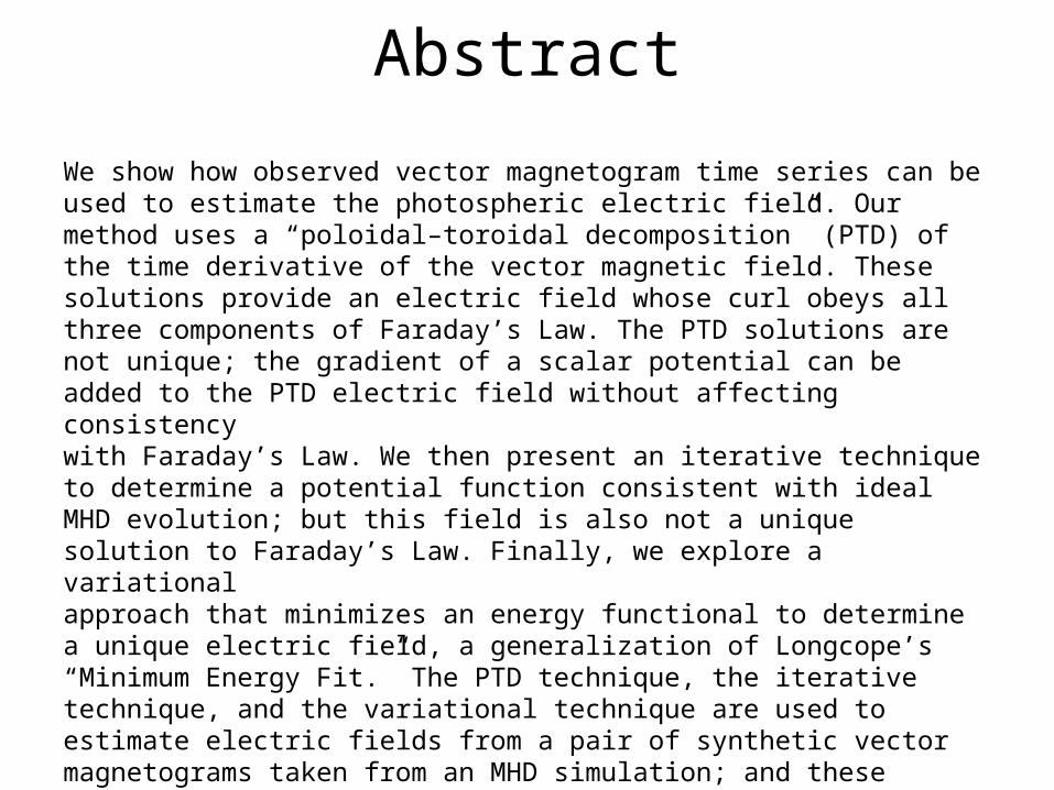
Abstract
We show how observed vector magnetogram time series can be used to estimate the photospheric electric field. Our method uses a “poloidal–toroidal decomposition” (PTD) of the time derivative of the vector magnetic field. These solutions provide an electric field whose curl obeys all three components of Faraday’s Law. The PTD solutions are not unique; the gradient of a scalar potential can be added to the PTD electric field without affecting consistencywith Faraday’s Law. We then present an iterative technique to determine a potential function consistent with ideal MHD evolution; but this field is also not a unique solution to Faraday’s Law. Finally, we explore a variationalapproach that minimizes an energy functional to determine a unique electric field, a generalization of Longcope’s “Minimum Energy Fit.” The PTD technique, the iterative technique, and the variational technique are used toestimate electric fields from a pair of synthetic vector magnetograms taken from an MHD simulation; and these fields are compared with the simulation’s known electric fields. The PTD and iteration techniques compare favorably to results from existing velocity inversion techniques. These three techniques are then applied to a pair of vector magnetograms of solar active region NOAA AR8210, to demonstrate the methods with real data.
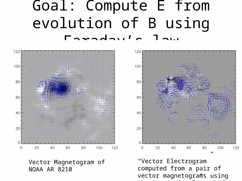
Goal: Compute E from evolution of B using Faraday’s law
Vector Magnetogram of NOAA AR 8210
“Vector Electrogram” computed from a pair of vector magnetograms using the “variational” method.
4
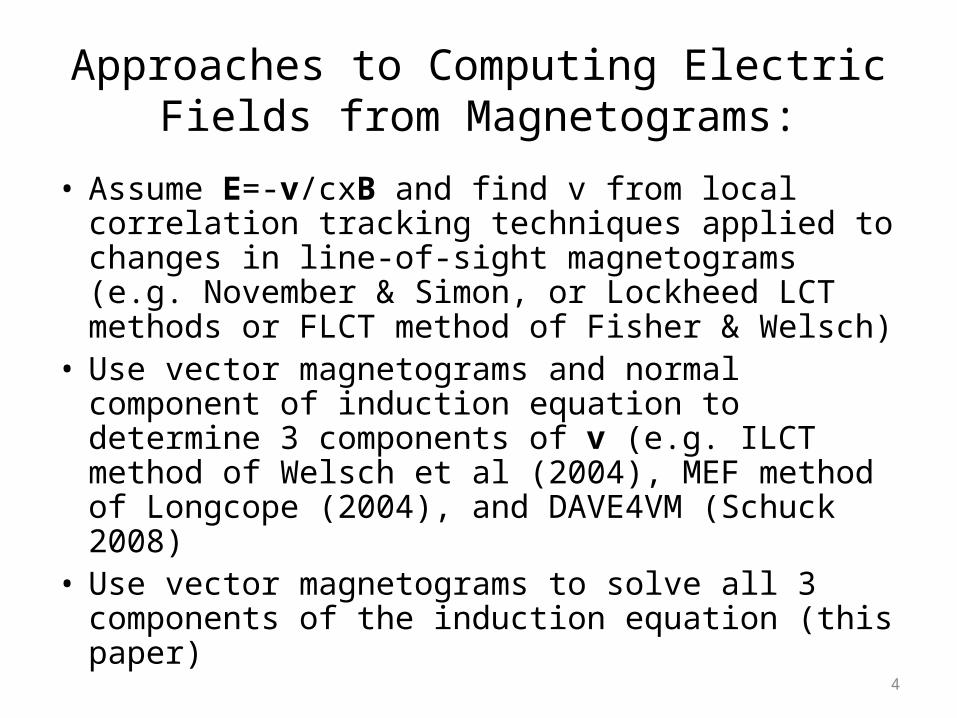
Approaches to Computing Electric Fields from Magnetograms:
• Assume E=-v/cxB and find v from local correlation tracking techniques applied to changes in line-of-sight magnetograms (e.g. November & Simon, or Lockheed LCT methods or FLCT method of Fisher & Welsch)
• Use vector magnetograms and normal component of induction equation to determine 3 components of v (e.g. ILCT method of Welsch et al (2004), MEF method of Longcope (2004), and DAVE4VM (Schuck 2008)
• Use vector magnetograms to solve all 3 components of the induction equation (this paper)
5
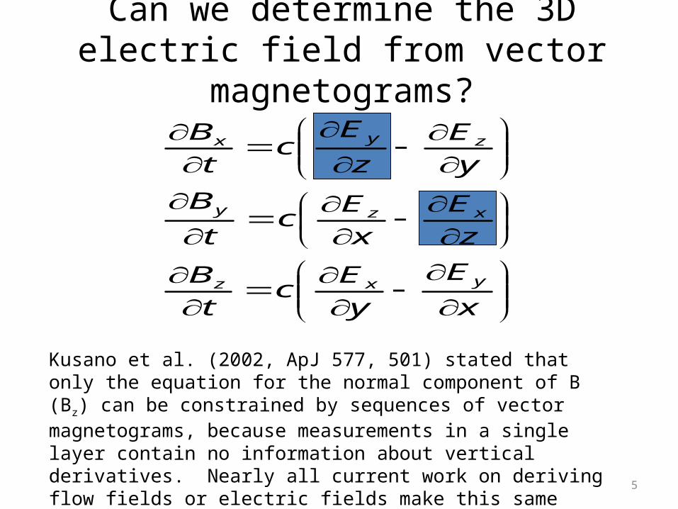
Can we determine the 3D electric field from vector magnetograms?
x
E
y
Ec
t
B
z
E
x
Ec
t
B
y
E
z
Ec
t
B
yxz
xzy
zyx
Kusano et al. (2002, ApJ 577, 501) stated that only the equation for the normal component of B (Bz) can be constrained by sequences of vector magnetograms, because measurements in a single layer contain no information about vertical derivatives. Nearly all current work on deriving flow fields or electric fields make this same assumption. But is this statement true?

6
The magnetic induction equation
One can then derive these Poisson equations relating the time derivative of the observed magnetic field B to corresponding time derivatives of the potential functions:
€
∇h2 ˙ β = − ˙ Β z (3);
∇ h2˙ J = −
4π ˙ J zc
= −ˆ z ⋅(∇ h × ˙ B h ) (4);
∇ h2 ∂ ˙ β
∂z
⎛
⎝ ⎜
⎞
⎠ ⎟=∇ h ⋅ ˙ B h (5)
Since the time derivative of the magnetic field is equal to -cxE, we can immediately relate the curl of E and E itself to the potential functions determined from the 3 Poisson equations:
€
B =∇×∇×βˆ z +∇ × Jˆ z (1)˙ B =∇ ×∇ × ˙ β ̂ z +∇ × ˙ J ̂ z (2)
Use the poloidal-toroidal decomposition of the magnetic field and its partial time derivative:
7
Relating xE and E to the 3 potential functions:
€
∇×E =−1
c∇ h
∂ ˙ β
∂z
⎛
⎝ ⎜
⎞
⎠ ⎟−
1
c∇ h × ˙ J ̂ z +
1
c∇ h
2 ˙ β ̂ z (6)
E =−1
c∇ h × ˙ β ˆ z + ˙ J ̂ z ( ) −∇ψ = EI −∇ψ (7)
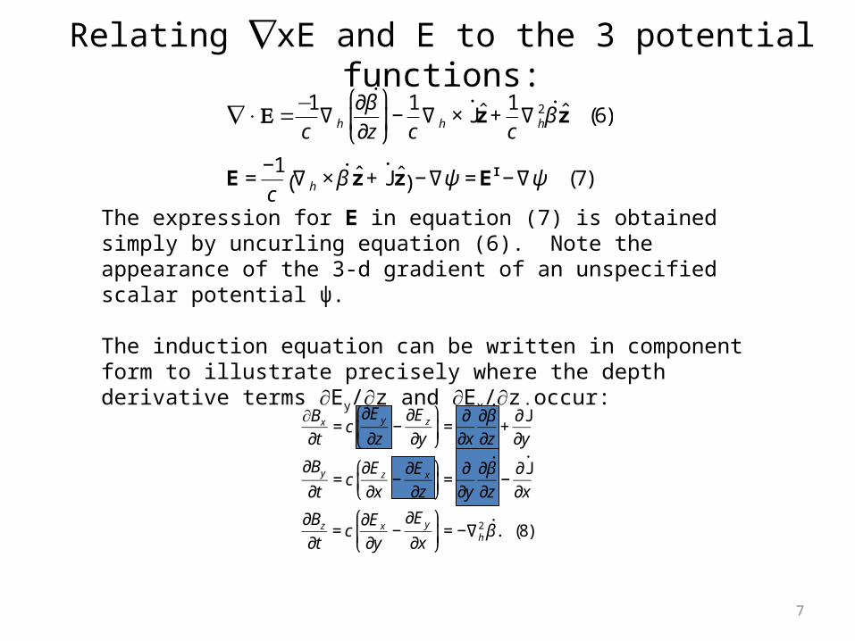
The expression for E in equation (7) is obtained simply by uncurling equation (6). Note the appearance of the 3-d gradient of an unspecified scalar potential ψ.
The induction equation can be written in component form to illustrate precisely where the depth derivative terms Ey/z and Ex/z occur:
€
∂Bx
∂t= c
∂Ey
∂z−
∂E z
∂y
⎛
⎝ ⎜
⎞
⎠ ⎟=
∂
∂x
∂ ˙ β
∂z+
∂˙ J
∂y
∂By
∂t= c
∂E z
∂x−
∂E x
∂z
⎛
⎝ ⎜
⎞
⎠ ⎟=
∂
∂y
∂ ˙ β
∂z−
∂˙ J
∂x
∂Bz
∂t= c
∂Ex
∂y−
∂E y
∂x
⎛
⎝ ⎜
⎞
⎠ ⎟= −∇h
2 ˙ β . (8)
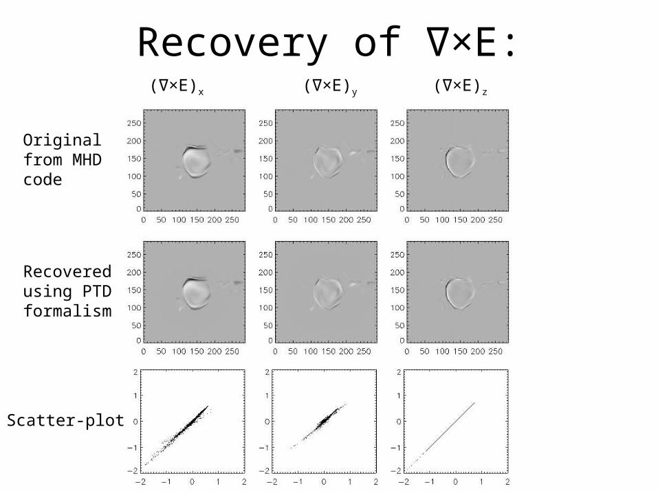
Recovery of ×E:∇
Original from MHD code
Recovered using PTD formalism
Scatter-plot
( ×E)∇ x ( ×E)∇ y ( ×E)∇ z
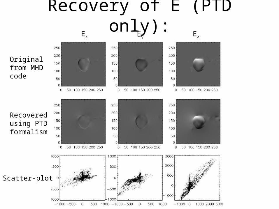
Recovery of E (PTD only):
Original from MHD code
Recovered using PTD formalism
Scatter-plot
Ex Ey Ez
10
Summary: excellent recovery of xE, only approximate recovery of E.
Why is this? The problem is that E, in contrast to xE, is mathematically under-constrained. The gradient of the unknown scalar potential in equation (7) does not contribute to xE, but it does contribute to E.
In the two specific cases just shown, the actual electric field originates largely from the ideal MHD electric field –v/c x B. In this case, E∙B is zero, but the recovered electric field contains significant components of E parallel to B. The problem is that the physics necessary to uniquely derive the input electric field is missing from the PTD formalism. To get a more accurate recovery of E, we need some way to add some knowledge of additional physics into a specification of ψ.
Next, we will now show how simple physical considerations can be used to derive constraint equations for ψ using an ad-hoc “iterative” approach.
11
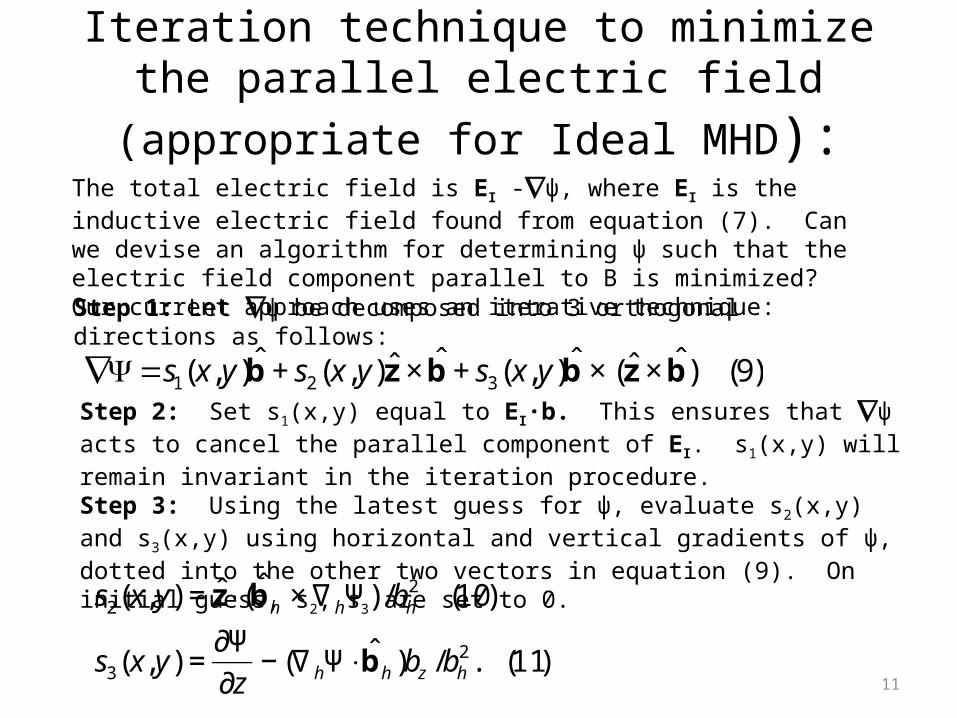
Iteration technique to minimize the parallel electric field (appropriate for Ideal MHD):
The total electric field is EI -ψ, where EI is the inductive electric field found from equation (7). Can we devise an algorithm for determining ψ such that the electric field component parallel to B is minimized? Our current approach uses an iterative technique:
€
s2(x, y) = ˆ z ⋅ ( ˆ b h ×∇hΨ) /bh2 (10)
s3(x, y) =∂Ψ
∂z− (∇hΨ⋅
ˆ b h )bz /bh2 . (11)
Step 1: Let ψ be decomposed into 3 orthogonal directions as follows:
€
∇Ψ=s1(x, y) ˆ b + s2(x, y)ˆ z × ˆ b + s3(x, y) ˆ b × (ˆ z × ˆ b ) (9)Step 2: Set s1(x,y) equal to EI∙b. This ensures that ψ acts to cancel the parallel component of EI. s1(x,y) will remain invariant in the iteration procedure.Step 3: Using the latest guess for ψ, evaluate s2(x,y) and s3(x,y) using horizontal and vertical gradients of ψ, dotted into the other two vectors in equation (9). On initial guess, s2, s3 are set to 0.
12
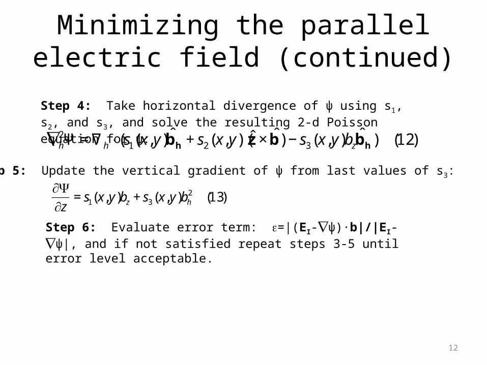
Minimizing the parallel electric field (continued)
Step 4: Take horizontal divergence of ψ using s1, s2, and s3, and solve the resulting 2-d Poisson equation for ψ:
€
∇h2Ψ =∇h ⋅ (s1(x, y) ˆ b h + s2(x,y)(ˆ z × ˆ b ) − s3(x, y)bz
ˆ b h ) (12)
Step 5: Update the vertical gradient of ψ from last values of s3:
€
∂Ψ∂z
= s1(x, y)bz + s3(x,y)bh2 (13)
Step 6: Evaluate error term: =|(EI-ψ)∙b|/|EI-ψ|, and if not satisfied repeat steps 3-5 until error level acceptable.
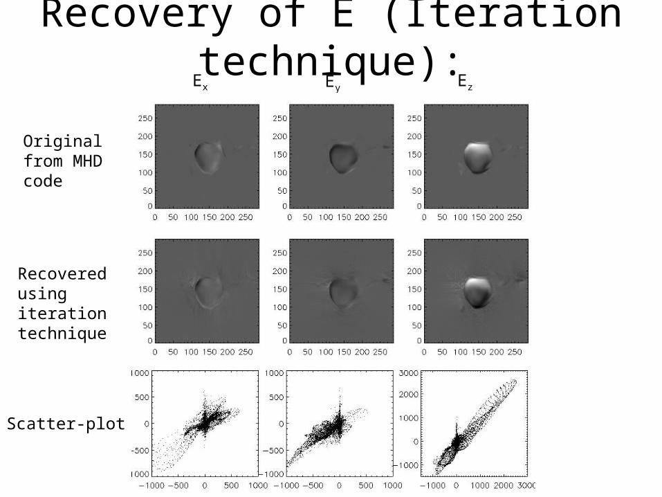
Recovery of E (Iteration technique):
Original from MHD code
Recovered using iteration technique
Scatter-plot
Ex Ey Ez
14
Another Approach to finding ψ: A Variational Technique
The electric field, or the velocity field, is strongly affected by forces acting on the solar atmosphere, as well as by the strong sources and sinks of energy near the photosphere. Here, with only vector magnetograms, we have none of this detailed information available to help us resolve the degeneracy in E from ψ.
One possible approach is to vary ψ such that an approximate Lagrangian for the solar plasma is minimized. The energy density for the electromagnetic field is E2+B2, for example. The contribution of the kinetic energy to the Lagrangian is ½ ρv2, which under the assumption that E = -v/c x B, means minimizing E2/B2. Since B is already determined from the data, minimizing the Lagrangian essentially means varying ψ such that E2 or E2/B2 is minimized. Here, we will allow for a more general case by minimizing W2E2 integrated over the magnetogram, where W2 is an arbitrary weighting function.
15
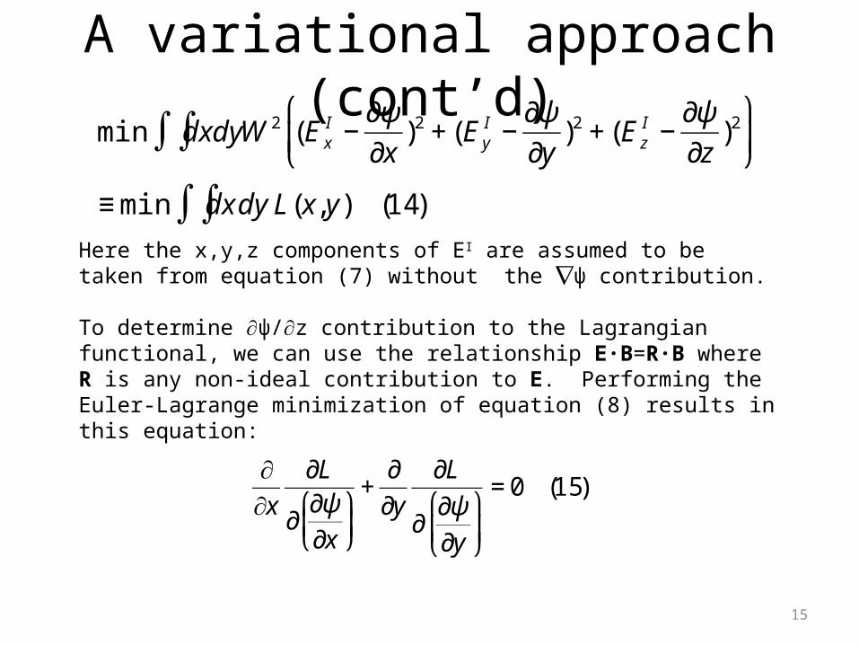
A variational approach (cont’d)
€
min dxdyW 2 (ExI −
∂ψ
∂x)2 + (Ey
I −∂ψ
∂y)2 + (E z
I −∂ψ
∂z)2
⎛
⎝ ⎜
⎞
⎠ ⎟∫∫
≡ min dx dy L(x,y)∫∫ (14)
Here the x,y,z components of EI are assumed to be taken from equation (7) without the ψ contribution.
To determine ψ/z contribution to the Lagrangian functional, we can use the relationship E B∙ =R B∙ where R is any non-ideal contribution to E. Performing the Euler-Lagrange minimization of equation (8) results in this equation:
€
∂∂x
∂L
∂∂ψ
∂x
⎛
⎝ ⎜
⎞
⎠ ⎟+
∂
∂y
∂L
∂∂ψ
∂y
⎛
⎝ ⎜
⎞
⎠ ⎟
= 0 (15)
16
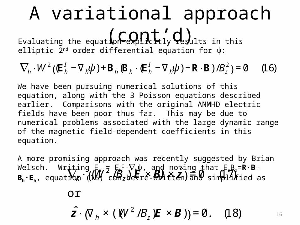
A variational approach (cont’d)
€
∇h ⋅W2 (Eh
I −∇hψ ) +Bh (Bh ⋅ (EhI −∇hψ ) −R⋅B) /Bz
2( ) = 0 (16)
Evaluating the equation explicitly results in this elliptic 2nd order differential equation for ψ:
We have been pursuing numerical solutions of this equation, along with the 3 Poisson equations described earlier. Comparisons with the original ANMHD electric fields have been poor thus far. This may be due to numerical problems associated with the large dynamic range of the magnetic field-dependent coefficients in this equation.
A more promising approach was recently suggested by Brian Welsch. Writing Eh = EhI-
hψ, and noting that EzBz=R B∙ -Bh E∙ h, equation (16) can be re-written and simplified as
€
∇h ⋅ (W 2 /Bz)(E × B) × ˆ z ( ) = 0 (17)
or
ˆ z ⋅ ∇h × ((W 2 /Bz )E × B)( ) = 0. (18)
17
A variational approach (cont’d)
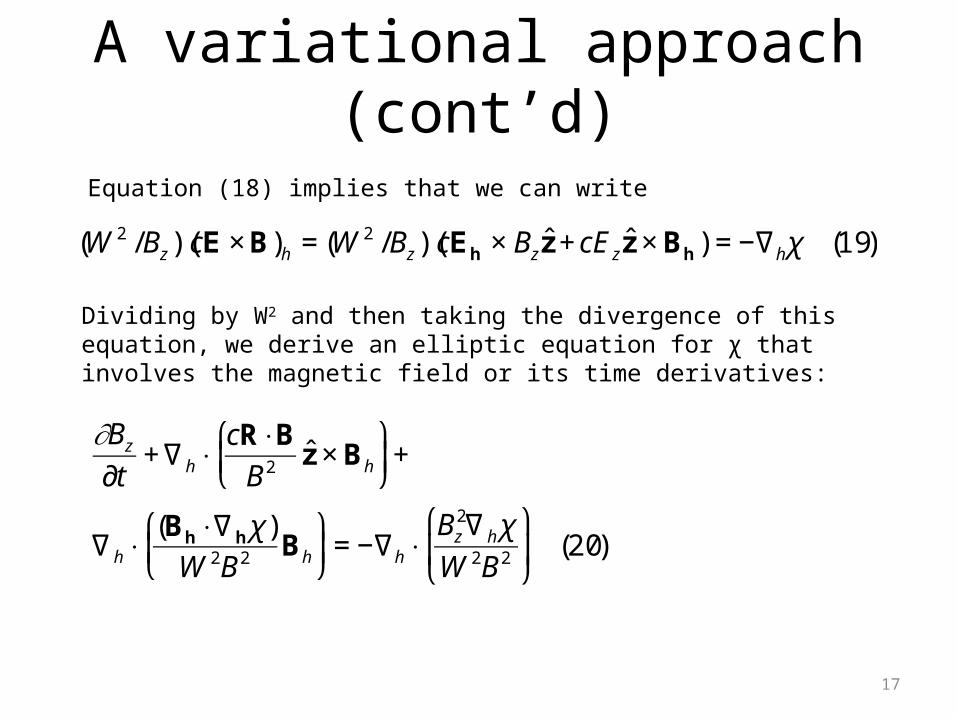
Equation (18) implies that we can write
€
(W 2 /Bz )(cE × B)h = (W 2 /Bz )(cEh × Bzˆ z + cE z
ˆ z × Bh ) = −∇hχ (19)
Dividing by W2 and then taking the divergence of this equation, we derive an elliptic equation for χ that involves the magnetic field or its time derivatives:
€
∂Bz
∂t+∇h ⋅
cR⋅B
B2ˆ z × Bh
⎛
⎝ ⎜
⎞
⎠ ⎟+
∇h ⋅(Bh ⋅ ∇h χ )
W 2B2 Bh
⎛
⎝ ⎜
⎞
⎠ ⎟= −∇h ⋅
Bz2∇h χ
W 2B2
⎛
⎝ ⎜
⎞
⎠ ⎟ (20)
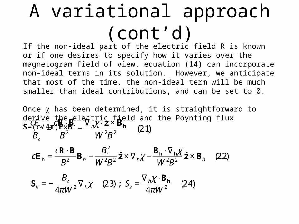
A variational approach (cont’d)If the non-ideal part of the electric field R is known or if one desires to specify how it varies over the magnetogram field of view, equation (14) can incorporate non-ideal terms in its solution. However, we anticipate that most of the time, the non-ideal term will be much smaller than ideal contributions, and can be set to 0.
Once χ has been determined, it is straightforward to derive the electric field and the Poynting flux S=(c/4π)ExB:
€
cE z
Bz
=cR⋅B
B2 −∇hχ⋅ z × Bh
W 2B2 (21)
€
cEh =cR⋅B
B2 Bh −Bz
2
W 2B2ˆ z ×∇hχ −
Bh ⋅ ∇hχ
W 2B2ˆ z × Bh (22)
€
Sh = −Bz
4πW 2 ∇h χ (23); Sz =∇h χ ⋅Bh
4πW 2 (24)
A variational approach (cont’d)
19
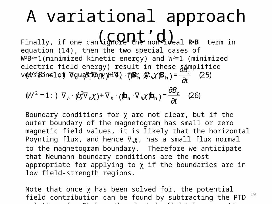
Finally, if one can ignore the non-ideal RB term in equation (14), then the two special cases of W2B2=1(minimized kinetic energy) and W2=1 (minimized electric field energy) result in these simplified versions of equation (14) for χ:
€
(W 2B2 =1:) ∇h ⋅ Bz2∇hχ( ) +∇h ⋅ Bh ⋅ ∇hχ( )Bh( ) =
∂Bz
∂t(25)
(W 2 =1:) ∇h ⋅ bz2∇hχ( ) +∇h ⋅ bh ⋅ ∇hχ( )bh( ) =
∂Bz
∂t(26)
Boundary conditions for χ are not clear, but if the outer boundary of the magnetogram has small or zero magnetic field values, it is likely that the horizontal Poynting flux, and hence ∇hχ, has a small flux normal to the magnetogram boundary. Therefore we anticipate that Neumann boundary conditions are the most appropriate for applying to χ if the boundaries are in low field-strength regions.
Note that once χ has been solved for, the potential field contribution can be found by subtracting the PTD solutions for EI from the electric field from equations (21-22).
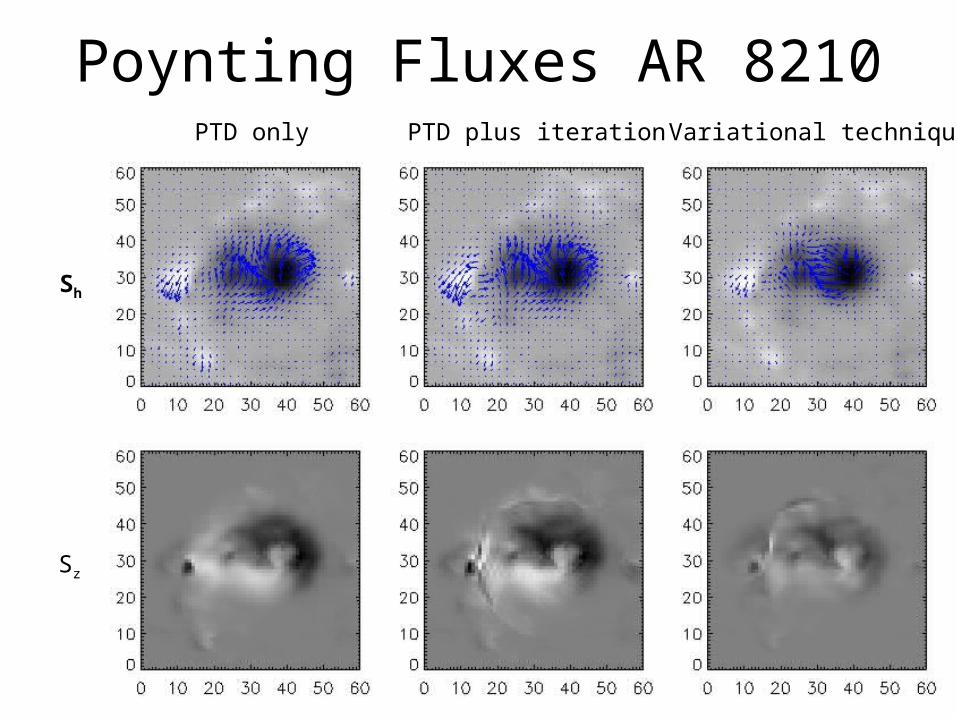
Poynting Fluxes AR 8210PTD only PTD plus iteration Variational technique
Sh
Sz

Summary of 3D electric field inversion
21
• It is possible to derive a 3D electric field from a time sequence of vector magnetograms which obeys all components of the Maxwell Faraday equation. This formalism uses the Poloidal-Toroidal Decomposition (PTD) formalism.
•The PTD solution for the electric field is not unique, and can differ from the true solution by the gradient of a potential function. The contribution from the potential function can be quite important.
•An equation for a potential function, or for a combination of the PTD electric field and a potential function, can be derived from iterative techniques and from a variational principle.