Estimating Consumption Economies of Scale,Adult Equivalence Scales, and Household

Bargaining Power

Martin BrowningDepartment of Economics,

Oxford University

Pierre-André ChiapporiDepartment of Economics,

University of Chicago

Arthur LewbelDepartment of Economics,

Boston College

Revised August 2006

Abstract

How much income would a woman living alone require to attain the same stan-dard of living that she would have if she were married? What percentage of a marriedcouple’s expenditures are controlled by the husband? How much money does a cou-ple save on consumption goods by living together versus living apart? We proposeand estimate a collective model of household behavior that permits identification andestimation of concepts such as these. We model households in terms of the utilityfunctions of its members, a bargaining or social welfare function, and a consump-tion technology function. We demonstrate generic nonparametric identification of themodel, and hence of a version of adult equivalence scales that we call "indifferencescales," as well as consumption economies of scale, the household’s resource sharingrule or members’ bargaining power, and other related concepts.

JEL codes: D11, D12, C30, I31, D63, J12. Keywords: Consumer Demand, Collective Model,Adult Equivalence Scales, Indifference Scales, Household Bargaining, Economies of Scale, De-mand Systems, Bargaining Power, Barten Scales, Sharing rule, Nonparametric Identification. Wewould like to thank the editor, anonymous referees, and Krishna Pendakur for numerous helpful

1

comments, and the Danish National Research Foundation for support through its grant to CAM.Corresponding Author: Arthur Lewbel, Department of Economics, Boston College, 140 Common-wealth Ave., Chestnut Hill, MA, 02467, USA. (617)-552-3678, lewbel@bc.edu, http://www2.bc.edu/~lewbel/

1 IntroductionOn average, how much income would a woman living alone require to attain the samestandard of living that she would have if she were married? What percentage of a marriedcouple’s expenditures benefit the husband? How much money does a couple save onconsumption goods by living together versus living apart? The goal of this paper is topropose a collective model of household behavior aimed at answering questions such asthese.

A large literature exists on specification and estimation of ordinary demand systems,collective and household bargaining models, and on identification (and lack thereof) ofequivalence scales, bargaining power measures, resource shares, consumption economiesscale, and other related household welfare measures. Some surveys of this literature in-clude Deaton and Muellbauer (1980), Blundell (1988), Browning (1992), Pollak and Wales(1992), Blundell, Preston, and Walker (1994), Blackorby and Donaldson (1994), Bour-guignon and Chiappori (1994), Lewbel (1997), Jorgenson (1997), Slesnick (1998), andVermeulen (2000).

We propose a new model of household consumption behavior that has three compo-nents, which are separate utility functions over goods for each household member, a con-sumption technology function that characterizes the jointness or publicness of goods andhence the economies of scale and scope in consumption, and a sharing rule that definesthe relative allocation of household resources among the household members. The basicstructure of this model is that households purchase a bundle (an n vector of quantities) ofgoods z. By economies of scale and scope in consumption, that is, by sharing, this z forthe household is equivalent to purchasing bundle of privately consumed goods x whereeach element of x is typically greater than or equal to the corresponding element of z. Thevector of quantities x is then divided up among the household members, and each memberi derives utility from consuming their bundle of goods xi , so the sum of these xi vectorsacross household members i is x . The conversion of z to x , which is embodied by theconsumption technology function, is essentially an application of the models of Barten(1964) and Gorman (1976) that characterize how demands differ across households of dif-ferent sizes. The allocation of shares of x to different household members, characterizedby a sharing rule, is essentially the collective household model of Bourguignon and Chiap-pori (1994) and Vermeulen (2000). Our model combines the features of both approaches,

2

which is what allows us to identify consumption economies of scale, adult equivalencescales, and household bargaining power.

We provide a dual representation of our collective model that facilitates empirical ap-plication, and show that the model is generically nonparametrically identified. We thenshow how the model overcomes traditional problems regarding nonidentification of equiv-alence scales, and can be used to address the questions listed above. Our results onlyrequire ordinal representations of preferences, and do not depend on any utility cardi-nalization or interpersonal comparability assumptions. We apply the model to Canadianconsumption data on couples and singles.

2 Equivalence Scales and Indifference ScalesEquivalence scales seek to answer the question, “how much money does a household needto spend to be as well off as a single person living alone?” Equivalence scales have manypractical applications. They are commonly used for generating poverty lines for house-holds of various compositions given a poverty line for single males. Income inequalitymeasures have been applied to equivalence scaled income rather than observed income toadjust for household composition (see, e.g., Jorgenson 1997). Calculation of appropriatelevels of alimony or life insurance also entail comparisons of costs of living for couplesversus those of singles.

An equivalence scale is traditionally defined as the expenditures of the household di-vided by the expenditures of a single person that enjoys the same “standard of living” asthe household. Just as a true cost of living price index measures the ratio of costs of attain-ing the same utility level under different price regimes, equivalence scales are supposed tomeasure the ratio of costs of attaining the same utility level under different household com-positions. Unfortunately, unlike true cost of living indexes, equivalence scales defined inthis way can never be identified from revealed preference data (that is, from the observedexpenditures of households under different price and income regimes). The reason is thatdefining a household to have the same utility level as a single individual requires that theutility functions of the household and of the single individual be comparable. We cannotavoid this problem by defining the household and the single to be equally well off whenthey attain the same indifference curve, analogous to the construction of true cost of livingindices, because the household and the single have different preferences and hence do notpossess the same indifference curves. Pollak and Wales (1979, 1992) describe these iden-tification problems in detail, while Blundell and Lewbel (1991) prove that only changes intraditional equivalence scales, but not their levels, can be identified by revealed preference.See Lewbel (1997) for a survey of equivalence scale identification issues.

3

We argue that the source of these identification problems is that the standard equiva-lence scale question is badly posed, for two reasons. First, by definition any comparisonbetween the preferences of two distinct decision units entails interpersonal utility compar-isons. Second, and perhaps more fundamental, the notion of a household utility is flawed.Individuals have utility, not households. What is relevant is not the ’preferences’ of a givenhousehold, but rather the preferences of the individuals that compose it.

We propose therefore that meaningful comparisons must be undertaken at the individ-ual level, and that the appropriate question to ask is, “how much income would an individ-ual living alone need to attain the same indifference curve over goods that the individualattains as a member of the household?” This latter question avoids issues of interpersonalcomparability and does not require us to compare the utility levels of different indiffer-ence curves. This question also does not depend on the utility level that is assigned to anindifference curve, i.e., it is unaffected by the fact that a person’s utility associated witha particular indifference curve over goods might change as a result of living with a part-ner. The question only depends on ordinal preferences, and hence is at least in principleanswerable from revealed preference data. Consequently, in sharp contrast with the exist-ing equivalence scale literature, our framework does not assume the existence of a uniquehousehold utility function, nor does it require comparability of utility between individualsand collectives (such as the household). Instead, following the basic ideas of the collec-tive approach to household behavior, we assume that each individual is characterized byhis/her own ordinal utility function, so the only comparisons we make is between the sameperson’s welfare (defined by indifference curves) in different living arrangements.

Define a equivalent income (or expenditure) to be the income or total expenditure levelyi∗ required by an individual household member i purchasing goods privately, to be aswell off materially as he or she is while living with others in a household that has jointincome y. In our model, this means that when the household spends y to buy a bundle z,household member i consumes a bundle xi (determined by the consumption technologyand sharing rule). Then yi∗ is the least expenditure required to buy a bundle of goods thatlies on member i’s same indifference curve as the bundle xi . Then, instead of a traditionaladult equivalence scale, we define individual i’s "indifference scale" to be Si = yi∗/y.

If member i were given the fraction Si of the household’s total expenditures, then bybuying goods on the open market individual i could get herself to the same indifferencecurve (defined in terms of her own utility function) that she attained as a member of thehousehold, taking into account whatever economies of scale in consumption she enjoyedby sharing and joint consumption within the household. Indifference scales depend onlyon the indifference curves of household members, the resources of the household, and onthe degree to which consumption is shared within the household, and so can be identifiedwithout any utility cardinalization or interpersonal comparability assumptions.

4

To see the usefulness of indifference scales, consider the question of determining anappropriate level of life insurance for a spouse. If the couple spends y dollars per year thenfor the wife to maintain the same standard of living after the husband dies, she will need aninsurance policy that pays enough to permit spending S f y dollars per year. Note that thisamount of money only compensates the wife enough to reach the same indifference curveover goods that she attained while she was a household member. It does not compensatefor any loss of utility due to grief, or for any change in her preferences that might resultfrom the death of her husband.

Similarly, in cases of wrongful death, juries are instructed to assess damages both tocompensate for the loss in “standard of living,” (i.e., Si ) and, separately for “pain andsuffering,” which would presumably be noneconomic effects (see Lewbel 2003). Anotherexample is poverty lines. If poverty lines for individuals have been established, then thepoverty line for a couple could be defined as the expenditures required for each memberof the couple to attain his or her own poverty line indifference curve.

Traditional equivalence scales do not properly answer these questions, because theyattempt to relate the utility of an individual to that of a household, instead of relating theutility of the same individual in two different settings, e.g. living with a husband versuswithout. This is similar to the distinction Pollak and Wales (1992) make between whatthey call a welfare comparison versus a situation comparison.

3 The ModelThis section describes the proposed household model. Let superscripts refer to householdmembers and subscripts refer to goods. Let Ui(xi) be the direct utility function for aconsumer i , consuming the vector of goods xi = (xi

1, ..., xin). We consider households

consisting of two members, which we will for convenience refer to as the husband (i = m)and the wife (i = f ). For many applications, it may be useful to interpret one of theseutility functions as a joint utility function for all but one member of the household, e.g.,U f could be the joint utility function of a wife and her children.

3.1 Household MembersASSUMPTION A1: Each household member i has a monotonically increasing, continu-ously twice differentiable and strictly quasi-concave utility function Ui(xi ) over a bundleof n goods xi .

If member i were to face an n vector of prices p with income level yi and this utilityfunction, he or she would solve the optimization program

5

maxxi

Ui (xi) subject to p xi = yi . (1)

Let xi = hi (p/yi) denote the solution to this individual optimization program, so thevector valued function hi is the set of Marshallian demand functions corresponding toUi (xi). Define V i by

V i(p/yi ) = Uihi(p/yi ) (2)

so V i is the indirect utility function corresponding to Ui . The functional form of individualdemand functions hi could be obtained from a functional specification of V i using Roy’sidentity.

3.2 The Household Decision ProcessNow consider a household consisting of a couple living together, and facing the budgetconstraint p z ≤ y. Following the standard collective approach, our key assumption re-garding decision making within the household is that outcomes are Pareto efficient. Astandard result of welfare theory (see, e.g., Bourguignon and Chiappori 1994) is that,given ordinality, one can without loss of generality write Pareto efficient decisions as aconstrained maximization of the weighted sum μU f (x f )+Um(xm). Here the constraintsare the technology constraints that define feasible values of individual consumption vec-tors x f and xm given z, and the budget constraint that defines feasible values of the vectorof purchases z. It is important to note that the Pareto weight μ may in general depend onprices, total expenditures, and on a vector s of distribution factors, the latter being definedas variables with no direct impact on preferences, technology or budget constraint, but thatmay influence the decision process.

We assume the household does not suffer from money illusion, and so write the Paretoweight function as μ(p/y, s). Possible examples of distribution factors s include individ-ual wages (as in Browning et al., 1994) or non labor income (Thomas 1990), sex ratio onthe relevant marriage market and divorce legislation (Chiappori, Fortin and Lacroix 2002),generosity of single parent benefits (Rubalcava and Thomas 2000), spouses’ wealth at mar-riage (Thomas, Contreras and Frankenberg 1997), and the targeting of specific benefits toparticular members (Duflo 2000). See also Chiappori and Ekeland (2005) for a generaldiscussion.

ASSUMPTION A2: Given budget and technology constraints and the absence of moneyillusion, the household makes Pareto efficient decisions, that is, it’s choice of x f and xm

6

maximizes the weighted sum U = μ(p/y, s)U f (x f ) + Um(xm). The Pareto weightfunction μ(p/y, s) is positive and twice continuously differentiable in p/y.

All of the functions we define may depend on other variables that we have suppressedfor notational simplicity. For example, in our empirical application the functions U f andUm also depend on demographic characteristics. We will also often similarly suppress thevector s.

In Assumption A2, U can be interpreted as a social welfare function for the house-hold, though one in which the relative effects of individual member’s utility functions mayvary with prices and distribution factors. Alternatively, U may stem from some specificbargaining model (Nash bargaining for instance), in which distribution factors affect indi-vidual threat points. This model also allows for effects such as a wife’s utility dependingon both her own attained utility level over goods (the value of U f ) and on her spouse’shappiness, Um .

From a bargaining perspective, the Pareto weight μ(p/y, s) can be seen as a measureof f ’s influence in the decision process. The larger the value of μ is, the greater is theweight that member f ’s preferences receive in the resulting household program, and thegreater will be the resulting private equivalent quantities x f versus xm . One difficulty withusing μ as a measure of the weight given to (or the bargaining power of) member f is thatthe magnitude of μ will depend on the arbitrary cardinalizations of the functions U f andUm . Later we will propose an alternative bargaining power measure, the sharing rule, thatdoes not depend upon any cardinalizations.

3.3 The Consumption Technology FunctionIn our model the household purchases some bundle z, but individual consumptions of thehousehold members add up to some other bundle x , with the difference due to sharing andjointness of consumption. In the technological relation z = F(x), we can interpret z asthe inputs and x as the outputs in the household’s consumption technology, described bythe production function F−1, though what is being ’produced’ is additional consumption.This framework is similar to a Becker (1965) type household production model, exceptthat instead of using the purchased vector of market goods z to produce commodities thatcontribute to utility, the household essentially produces the equivalent of a greater quantityof market goods x via sharing. The unobserved n vectors x f , xm , and x = x f + xm areprivate good equivalent vectors, that is, they are respectively the quantities of transformedgoods that are consumed by the female, the male, and in total.

ASSUMPTION A3: Given a purchased bundle of goods z, the feasible set of privategood equivalent bundles x f and xm are given by the consumption technology function

7

z = F(x f + xm).

It will often be convenient to work with a linear consumption technology, which ismathematically identical to Gorman’s (1976) linear technology (a special case of which isBarten (1964) scaling), except that we apply it in the context of a collective model.

ASSUMPTION A4: The consumption technology function is linear, so F(x) = Ax+a,where A is a nonsingular n by n matrix and a is a n vector.

Most of our theoretical results and all of our empirical work use a linear consumptiontechnology, but in an appendix we will show how our main identification and dualityresults can be generically extended to arbitrary smooth consumption technologies.

Consider some examples. Let good j be food. Suppose that if an individual or a couplebuy a quantity of food z j , the then total amount of food that the individual or couple canactually consume (that is, get utility from) is z j−a j , where a j is waste in food preparation,spoilage, etc.,. If the individuals lived apart, each would waste an amount a j , so the totalamount wasted would be 2a j , while living together results in only a waste of a j . Inthis simple example the economies of scale to food consumption from living together area reduction in waste from 2a j to a j , implying that x j = z j + a j , so the consumptiontechnology function for food takes the simple form z j = Fj(x) = x j − a j .

Economies of scale also arise directly from sharing. For example, let good j be auto-mobile use, measured by distance traveled (or some consumed good that is proportionalto distance, perhaps gasoline). If x f

j and xmj are the distances traveled by car by each

household member, then the total distance the car travels is z j = (x fj + xm

j )/(1 + r),where r is the fraction of distance that the couple ride together. This yields a consumptiontechnology function for automobile use of z j = Fj (x) = x j/(1 + r). This example issimilar to the usual motivation for Barten (1964) scales, but it is operationally more com-plicated, because Barten scales fail to distinguish the separate utility functions, and hencethe separate consumptions, of the household members.

More complicated consumption technologies can arise in a variety of ways. The frac-tion of time r that the couple share the car could depend on the total usage, resulting inFj being a nonlinear function of x j . There could also be economies (or diseconomies) ofscope as well as scale in the consumption technology, e.g., the shared travel time percent-age r could be related to expenditures on vacations, resulting in Fj (x) being a function ofother elements of x in addition to x j .

The model also allows for possible diseconomies of scale, e.g., diagonal elements ofA could be larger than one or elements of a could be negative.

In the collective model literature sharing and jointness of consumption is usually mod-eled by assuming some goods are purely private and others purely public (see, e.g., Ver-

8

meulen 2000), with additional generality obtained by defining some goods to be the sumof public and private components, e.g., solo car travel and joint car travel could be mod-eled as two separate goods, one private and one public. Recalling that x j = x f

j + xmj ,

in our model a purely private good has z j = x j = x fj + xm

j , while a purely public goodwould have z j = x j/2, with the additional constraint that x f

j = xmj . Our model includes

both z j = x j and z j = x j/2 as special cases, and so includes purely private goods and canat least approximate purely public goods, but we do not impose the constraint x f

j = xmj .

Such constraints can be imposed in our model, but doing so would interfere with the sim-ple duality results we derive that make our model empirically tractable. We later showhow our model can be extended to include purely public goods and other, more generalconsumption technologies.

Goods that are often cited as purely public, such as heating, may actually be consumedin different quantities by different household members, as our model permits. For examplea spouse that stays at home consumes more of the household’s heat than one that goes to ajob in the daytime. Finally, we note that even a linear technology function F includes manytypes of joint and shared consumption that cannot be captured by models that only considerpurely private and purely public goods (such as economies of scope to consumption),and that our model produces household demand functions that nest as special cases theBarten (1964) and Gorman (1976) models, which are widely used in the empirical demandmodeling literature.

3.4 The Household’s programASSUMPTION A5: The household faces the budget constraint p z ≤ y.

Here z is the vector of quantities of the n goods the household purchases, p is marketprices and y is the household’s total expenditures. Assumptions A2, A3, and A5 togethersay that the household’s consumption behavior is determined by the optimization program

maxx f ,xm,z

μ(p/y)U f (x f )+Um(xm) subject to x = x f + xm , z = F(x), p z = y (3)

To save notation we have suppressed distribution factors s that affect the Pareto weight μand any demographic or other attributes that may affect μ or the utility functions U f andUm or the consumption technology F . The solution of the program (3) yields the house-hold’s demand functions, which we denote as z = h(p/y), and private good equivalentdemand functions xi = xi(p/y).

One way to interpret the program (3) is to consider two extreme cases. If all goods wereprivate and there were no shared or joint consumption, then F(x) = x , so z would equal

9

x f + xm and the program (3) would reduce to maxx f ,z μ(p/y)U f (x f ) + Um(z − x f )such that p z = y, which is the standard specification of a collective model for purelyprivate goods (see, e.g., Bourguignon and Chiappori 1994 or Vermeulen 2000). At theother extreme, imagine a household that has a consumption technology function F , butassume that the household’s utility function for transformed goods just equaled Um(x),as might happen if the male were a dictator that forced the other household members toconsume goods in the same proportion that he does. In that case, the model would reduceto maxz Um F−1(z) such that p z = y, which for linear F (Assumption A4) is equivalentto Gorman’s (1976) general linear technology model, a special case of which is Barten(1964) scales (corresponding to A diagonal and a zero). Our general model, program(3), combines the consumption technology logic of the Gorman or Barten framework withthe collective model of a household as either a bargaining or a social welfare maximizinggroup.

3.5 DualityTo prove identification results and to facilitate empirical application of our model, we de-rive a dual representation of the household’s program. To do so, consider the householdas an open economy. From the second welfare theorem, any Pareto efficient allocationcan be implemented as an equilibrium of this economy, possibly after lump sum transfersbetween members. We summarize these transfers by the sharing rule η(p/y), which is de-fined as the fraction of a suitably constructed measure of household resources consumedby member f . The household’s behavior is equivalent to allocating the fraction η(p/y) ofresources to member f , and the fraction 1 − η(p/y) to member m. Each member i thenmaximizes their own utility function Ui given a Lindahl (1919) type shadow price vectorπ and their own shadow income ηi to calculate their desired private good equivalent con-sumption vectors x f and xm . This concept of a sharing rule is borrowed directly from thecollective model literature (see, e.g., Browning and Chiappori 1998 and Vermeulen 2000for a survey), though our model is richer than these earlier households models because ofthe inclusion of the consumption technology function. Formally:

PROPOSITION 1: Let Assumptions A1, A2, A3, and A5 hold. There exists a Lindahlshadow price vector π(p/y) and a scalar valued sharing rule η(p/y), with 0 ≤ η(p/y) ≤1, such that

10

x f (p/y) = h f π(p/y)η(p/y)

xm(p/y) = hm π(p/y)1− η(p/y) (4)

z = h(p/y) = Fx f (p/y)+ xm(p/y)

This and other propositions are proved in the Appendix. Here π (p/y) denotes a vectorof equilibrium (shadow) prices within the household economy. One feature of this resultthat will be used later for identification and empirical tractability is that these shadowprices are the same for both household members. This follows from assuming consump-tion technologies of the form z = F(x f + xm). Our conceptual framework can be imme-diately extended to arbitrary technologies z = F∗(x f , xm), but we would then lose thisfeature of members facing the same shadow prices.

Without loss of generality, shadow prices are scaled so to make total shadow income ofthe household be π (x f + xm) = 1. The sharing rule η is then given by η = π x f , whichis the fraction of total shadow income consumed by member f . It follows that η(p/y) is adirect measure of the weight given to member f in the outcome of the household decisionprocess. The following proposition shows the relationship between the sharing rule η andthe Pareto weight μ.

PROPOSITION 2: Let Assumptions A1, A2, A3, and A5 hold, so by Proposition 1, thefunctions η(p/y) and π(p/y) exist. Then

μ(p/y) = −⎡⎣∂V m π(p/y)

1−η(p/y)∂η

⎤⎦ /⎡⎣∂V f π(p/y)

η(p/y)

∂η

⎤⎦ (5)

Given utility functions Ut and Um and a technology F , Proposition 1 shows thereexists a unique sharing rule function η(p/y) corresponding to any Pareto weight functionμ(p/y) and Proposition 2 shows the converse. Our model does not require identificationor estimation of μ (since we use η as our measure of resource allocation or bargainingpower), however, if one wanted to use Proposition 2 empirically to recover μ, one wouldneed variation in η that keeps π fixed. For that purpose, it suffices that η(p/y) dependon some parameter that can be varied holding shadow prices π(p/y) fixed. Distribution

11

factors s are obvious candidates. In general, shadow prices will depend in a complicatedway on the consumption technology function, on both members’ demand functions andon distribution factors. In particular, changing the members’ respective bargaining powerswill generally affect shadow prices because it modifies the structure of household demandand shadow prices are not independent of this structure. There is, however, an interestingexception to this rule, which is that π (p/y) has a simple tractable functional form thatonly depends on the consumption technology when that technology is linear (AssumptionA4), as follows.

PROPOSITION 3: Let Assumptions A1, A2, A3, A4, and A5 hold. Then Propositions1 and 2 hold with

π(p/y) = A py − a p

z = h(p/y) = Ah f A py − a p

1η(p/y)

+ Ahm A py − a p

11− η(p/y) + a. (6)

4 IdentificationGiven functional forms for the consumption technology function, the sharing rule, andmember demand functions, Proposition 1 shows how the demand functions for householdswould be constructed. In the case of linear consumption technologies, these householddemands have the simple, explicit form given in Proposition 3. Specifically, given lineartechnologies a simple parametric modeling strategy is to posit functional forms for indirectutility functions of members, and a functional form for the sharing rule η. Roy’s identitythen gives functional forms for the household member demand functions h f and hm , andthe resulting functional form for the demand functions of couples is given by equation (6).

While this result is convenient for empirical work, it would be useful to know if all thefeatures of our model are nonparametrically identified, since it would be undesirable if ourestimates of economies of scale, bargaining power, indifference scales, etc.,. were based inpart on untestable parametric assumptions. The question is, given the observable demandfunctions hm, h f , and h, can we identify (and later, estimate) the consumption technologyfunction F(x), the shadow prices π(p/y), the sharing rule η(p/y), and the private goodequivalent demand functions x f (p/y) and xm(p/y)? We show below that these functionsare ’generically’ nonparametrically identified, meaning that identification will only fail ifthe utility and technology functions are too simple (for example, a linear F is not identifiedif demands are of the linear expenditure system form). This identification in turn impliesnonparametric identification of objects of interest such as bargaining power, economies ofscale, and our indifference scales.

12

Two concepts that are relevant for identification are private goods and assignable goods.Define a good j to be private, or privately consumed, if z j = x j , so private goods haveno economies or diseconomies of scale in consumption. Define a good j to be assignableif x f

j and xmj are observed, so assignable goods are goods where we know how much is

consumed separately by the husband and by the wife. For example, if we observe howmuch time each household member uses the family car then auto use is assignable (andnot necessarily private, since some of that usage is shared when they ride together). Cloth-ing is private if we observe total purchases of clothing and there are no economies ordiseconomies of scale or scope in clothing use. Clothing is both private and assignableif it is private and if we separately observe husbands’ clothing use and wives’ clothinguse. Having some goods be private and/or assignable helps identification, by reducing theinformation required to go from purchases z j to private good equivalent consumptions x f

jand xm

j .

4.1 Generic IdentificationASSUMPTION A6: The household demand function h(·) and the household member de-mand functions h f (·) and hm(·) are identified.

Identification of the household demand function is straightforward, since we wouldgenerally estimate z = h(p/y) using ordinary demand data on observed prices p, total ex-penditures y, and corresponding bundles z purchased by couples. Identification of memberdemand functions h f and hm is not immediate, but can be obtained in a few different ways.If individual’s indifference curves over goods do not change when they marry or otherwiseform households, then h f and hm could be estimated (and hence identified) using ordinarydemand data on observed prices, total expenditures, and quantities purchased by individualmen and women living alone, that is, from observing the consumption demands of singles.More generally, h f and hm can be identified if preferences do change upon marriage, aslong as those changes can be identified, since in that case we can use singles data, couplesdata, and knowledge of the changes (e.g., estimated parameters that change values aftermarriage) to recover h f and hm .

Identification could alternatively be obtained if we can directly observe the consump-tion of goods by each individual within the household under various price and expendi-ture regimes, since that would provide direct observation of the functions xm(p/y) andx f (p/y) along with h(p/y), which could be used to recover h f and hm . In other words,h f and hm will be identified if goods are assignable.

In practice, identification and associated estimation of h f and hm may be obtained bysome mix of all of the above, e.g., h f and hm may be identified from a combination of

13

estimated demand functions of singles and of couples, parameterization of changes in pref-erences over goods resulting from marriage, and make use of assignability of some goods,such as separate observation of men’s and women’s clothing purchases in the household.We will later illustrate these identification methods in the context of an empirical applica-tion.

Older demand models such as Barten (1964), Gorman (1976), and Lewbel (1985), andnewer specifications such as shape invariance (see, e.g., Pendakur (1999)) are models ofhow demands vary across households of different sizes, and so exploit data from bothsingles and couples to jointly identify parameters that are common to both, as well asidentifying parameters that characterize the differences between the two. The idea of usingsingles data to identify some couple’s parameters has also been used in some labor supplymodels, including Barmby and Smith (2001) and Bargain et. al. (2004). An exampleof using smoothness assumptions to identify features of individual household memberconsumptions is Chesher (1998).

Ordinary revealed preference theory shows that the utility functions of members Um

and U f , or equivalently the indirect utility functions V m and V f , are identified up toarbitrary monotonic transformation given the member demand functions h f and hm . Ourgoal now is to use the additional information of observed household demand functions hto identify the other features of the household’s program.

PROPOSITION 4: Let Assumptions A1, A2, A3, A4, A5, and A6 hold. If the number ofgoods in the system is n ≥ 3, then the functions π(p/y), η(p/y), xm(p/y) and x f (p/y),and the technology parameters represented by A and a, are all generically identified.

The Pareto weight μ(p/y) depends upon the unobservable cardinalization of memberutilities, but if those cardinalizations are known and distribution factors are present, thenμ(p/y) may also be identified using equation (5), given Propositions 2 and 3.

The identification in Proposition 4 is only generic, in the sense that it only shows thatwe have (many) more equations than unknowns. However these equations (equation (24)in the appendix for t = 1, ..., T ) could fail to be linearly independent for particular func-tional forms (roughly analogous to the order versus the rank condition for identificationin traditional linear simultaneous systems). For example, it can be readily verified thatidentification fails when the individual demands h f and hm have the Linear ExpenditureSystem functional form. However, such problems disappear for sufficiently complicatedfunctional forms for members demands, since nonlinearities in functional form tend toeliminate linear dependencies across equations. This is demonstrated in the next sub-section with the Almost Ideal (AIDS) and Quadratic Almost Ideal (QUAIDS) functionalforms. The latter will be used for our empirical estimation.

14

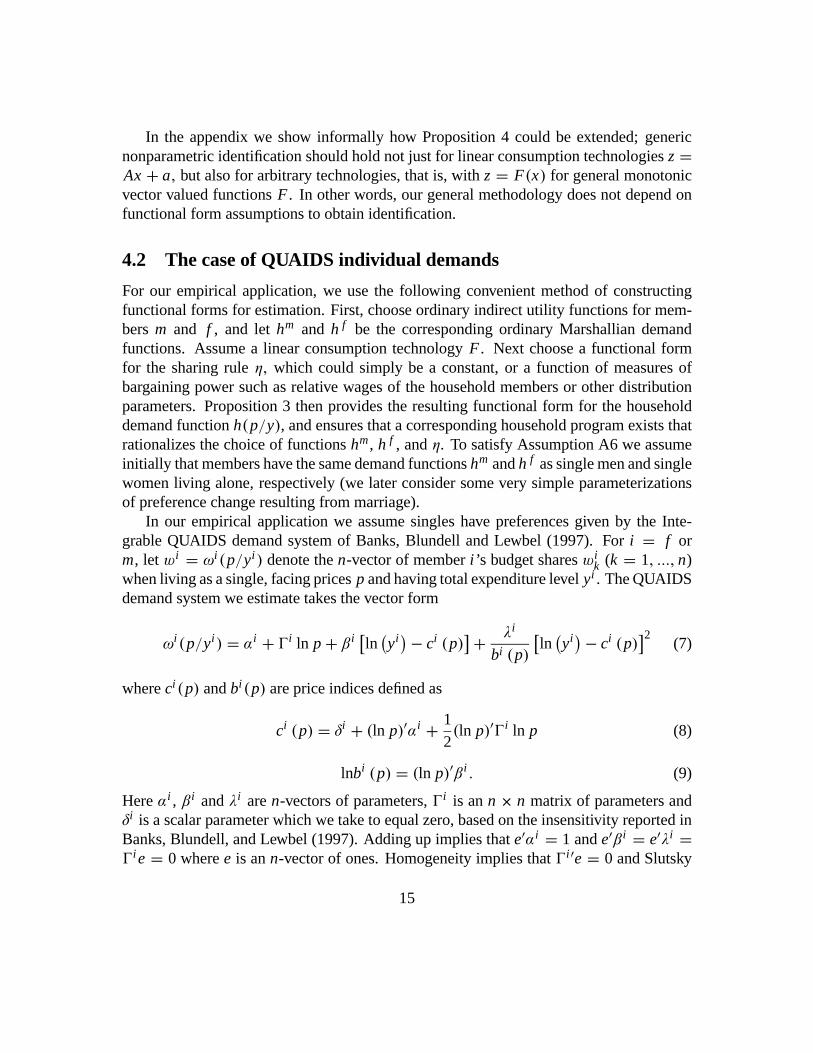
In the appendix we show informally how Proposition 4 could be extended; genericnonparametric identification should hold not just for linear consumption technologies z =Ax + a, but also for arbitrary technologies, that is, with z = F(x) for general monotonicvector valued functions F . In other words, our general methodology does not depend onfunctional form assumptions to obtain identification.

4.2 The case of QUAIDS individual demandsFor our empirical application, we use the following convenient method of constructingfunctional forms for estimation. First, choose ordinary indirect utility functions for mem-bers m and f , and let hm and h f be the corresponding ordinary Marshallian demandfunctions. Assume a linear consumption technology F . Next choose a functional formfor the sharing rule η, which could simply be a constant, or a function of measures ofbargaining power such as relative wages of the household members or other distributionparameters. Proposition 3 then provides the resulting functional form for the householddemand function h(p/y), and ensures that a corresponding household program exists thatrationalizes the choice of functions hm , h f , and η. To satisfy Assumption A6 we assumeinitially that members have the same demand functions hm and h f as single men and singlewomen living alone, respectively (we later consider some very simple parameterizationsof preference change resulting from marriage).

In our empirical application we assume singles have preferences given by the Inte-grable QUAIDS demand system of Banks, Blundell and Lewbel (1997). For i = f orm, let wi = ωi(p/yi ) denote the n-vector of member i’s budget shares wi

k (k = 1, ..., n)when living as a single, facing prices p and having total expenditure level yi . The QUAIDSdemand system we estimate takes the vector form

ωi (p/yi) = αi + i ln p + βi ln yi − ci (p) + λi

bi (p)ln yi − ci (p) 2 (7)

where ci(p) and bi(p) are price indices defined as

ci (p) = δi + (ln p) αi + 12(ln p) i ln p (8)

lnbi (p) = (ln p) βi . (9)

Here αi , βi and λi are n-vectors of parameters, i is an n × n matrix of parameters andδi is a scalar parameter which we take to equal zero, based on the insensitivity reported inBanks, Blundell, and Lewbel (1997). Adding up implies that e αi = 1 and e βi = e λi =

i e = 0 where e is an n-vector of ones. Homogeneity implies that i e = 0 and Slutsky

15

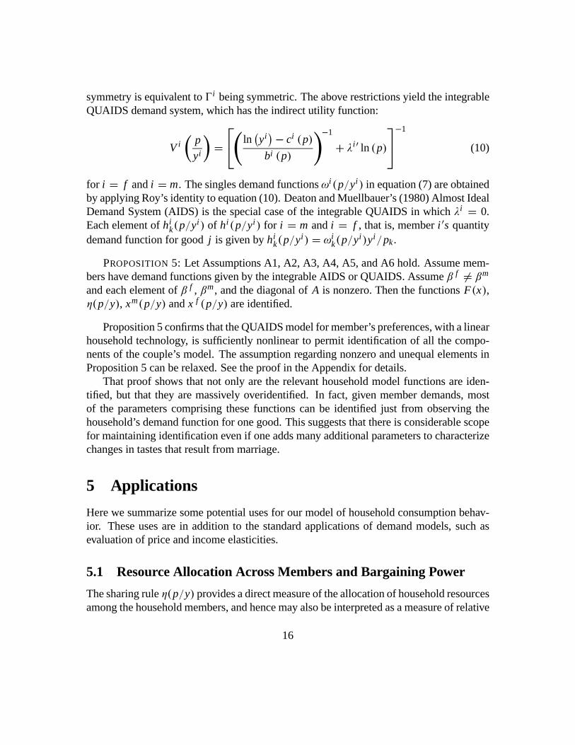
symmetry is equivalent to i being symmetric. The above restrictions yield the integrableQUAIDS demand system, which has the indirect utility function:

V i pyi =

⎡⎣ ln yi − ci (p)bi (p)

−1

+ λi ln (p)

⎤⎦−1

(10)

for i = f and i = m. The singles demand functions ωi(p/yi ) in equation (7) are obtainedby applying Roy’s identity to equation (10). Deaton and Muellbauer’s (1980) Almost IdealDemand System (AIDS) is the special case of the integrable QUAIDS in which λi = 0.Each element of hi

k(p/yi) of hi(p/yi) for i = m and i = f , that is, member i s quantity

demand function for good j is given by hik(p/y

i) = ωik(p/y

i)yi/pk .

PROPOSITION 5: Let Assumptions A1, A2, A3, A4, A5, and A6 hold. Assume mem-bers have demand functions given by the integrable AIDS or QUAIDS. Assume β f = βm

and each element of β f , βm , and the diagonal of A is nonzero. Then the functions F(x),η(p/y), xm(p/y) and x f (p/y) are identified.

Proposition 5 confirms that the QUAIDS model for member’s preferences, with a linearhousehold technology, is sufficiently nonlinear to permit identification of all the compo-nents of the couple’s model. The assumption regarding nonzero and unequal elements inProposition 5 can be relaxed. See the proof in the Appendix for details.

That proof shows that not only are the relevant household model functions are iden-tified, but that they are massively overidentified. In fact, given member demands, mostof the parameters comprising these functions can be identified just from observing thehousehold’s demand function for one good. This suggests that there is considerable scopefor maintaining identification even if one adds many additional parameters to characterizechanges in tastes that result from marriage.

5 ApplicationsHere we summarize some potential uses for our model of household consumption behav-ior. These uses are in addition to the standard applications of demand models, such asevaluation of price and income elasticities.

5.1 Resource Allocation Across Members and Bargaining PowerThe sharing rule η(p/y) provides a direct measure of the allocation of household resourcesamong the household members, and hence may also be interpreted as a measure of relative

16

bargaining power after taking altruism into account. If all goods were private, with noeconomies of scale or scope in consumption (i.e., if x = z) then η would exactly equalthe share of total expenditures y that were used to purchase the bundle x f consumed bymember f . Browning and Chiappori (1998), using household data alone, show that therelative bargaining power measures can only be identified up to an arbitrary location. Bycontrast, Propositions 4 and 5 show that in our model, by combining demand functionsof households and the demand functions of individual members, the sharing rule η iscompletely identified.

We argue that the Pareto weight μ is a less tractable measure of bargaining powerthan η, because μ depends on the unobservable cardinalizations of the utility functionsof individual household members, while η is recoverable just from observable demandfunctions. However, if these cardinalizations are known, then μ(p/y) can be calculatedand used with our model.

5.2 Economies of Scale in ConsumptionPrevious attempts to measure economies of scale in consumption have required very re-strictive assumptions regarding the preferences of household members (see, e.g., Nelson1988). In contrast, given estimates of the private good equivalents vector x = x f + xm

from our model, we may calculate y/p x , which is a measure of the overall economies ofscale from living together, since y is what the household spends to buy z and p x is thecost of buying the private good equivalents of z. This economy of scale measure takes theform y

p x= y

p h f π/η + hmπ/(1− η) .

This measure does not directly provide an estimate of adult equivalence scales or indif-ference scales. The reason is that, in general, the shadow prices used within the householdare not proportional to market prices (this is exactly Barten’s intuition). It follows thatindividuals living alone would not buy the bundles x f and xm , which were optimal givenshadow prices They would in general reach a higher level of utility by re-optimizing usingmarket instead of shadow prices.

We may also calculate the corresponding economies of scale in consumption for eachgood k separately as zk/xk . This can also be interpreted as a measure of the publicnessor privateness of each good. For a purely private good with no jointness of consumption,zk/xk equals one, while goods that are mostly shared will have zk/xk close to one half.When the consumption technology has the Barten form, zk/xk equals the Barten scale forgood k.

17

5.3 Indifference ScalesGiven each household member i’s private good equivalents xi , we define member i’s col-lective based equivalent income, yi∗, as the minimum expenditures required to buy a vectorof goods that is on the same member i indifference curve as xi . The ratio Si = yi∗/y isthen what we call member i’s indifference scale, so Si is the fraction of the household’sincome that member i would need to buy a bundle of privately consumed goods at marketprices that put her on the same indifference curve over goods that she attained as a memberof the household.

Like the above described economies of scale and bargaining power measures, theseindifference scales do not depend on any utility cardinalizations or assumptions of inter-personally comparable utility.

Recall that V f (p/y f ) is the indirect utility function of member f , and the private goodequivalent vector consumed by member f in the household is x f (p/y) = h f π(p/y)/η(p/y) ,where h f is the Marshallian demand function obtained from V f (p/y f ) by Roy’s identity.The indifference scale S f (p/y, η) is defined as the solution to the equation

V f p/yS f (p/y, η)

= V f π(p/y)η

(11)

This definition of S f (p/y, η) only depends upon an ordinal representation of utility, i.e.,it does not depend on the chosen cardinalization for member f ’s utility function. Specifi-cally, and in marked contrast to traditional adult equivalence scales, replacing V f with anymonotonic transformation of V f in equation (11) leaves S f unchanged. The expressionfor member m defining Sm , is the same as equation (11), replacing f with m and replacingη with 1− η.

As discussed earlier, these indifference scales Si(p/y, η) could be used for poverty, lifeinsurance, and wrongful death, calculations. For example, in the case of a wrongful deathor insurance calculation, a woman (or a mother and her children, if V f is defined as thejoint utility function of a mother and her children) would need income Si(p/y, η(p/y))yto attain the same standard of living without her husband that she (or they) attained whilein the household with the husband present and total expenditures y. This would take intoaccount the share of household resources η(p/y) that she consumed, and would be ex-actly sufficient to compensate for the loss of economies of scale and scope from sharedconsumption, but would not compensate her for the husband’s consumption, or for griev-ing, loss of companionship, or other components of utility that are assumed to be separablefrom consumption of goods. It would also not compensate for any change in preferencesover goods that might occur as a result of the death.

Another interesting indifference scale to construct is S f (p/y, η)/Sm(p/y, 1− η), theratio of how much income a woman needs when living alone to the income a man needs

18

when living alone to make each as well off as they would be in a household. Even if menand women had identical preferences, this ratio need not equal one, because if the sharingrule η is bigger than one half, then the wife receives more than half of the household’s re-sources, and hence would need more income when living alone to attain the same standardof living. To separate bargaining effects from other considerations, one might instead cal-culate Si(p/y, 1/2), which is the indifference scale assuming equal sharing of resources.For example, the ratio S f (p/y, 1/2)/Sm(p/y, 1/2) might better match the intuition of anequivalence scale comparing women to men.

In other applications, one might want to consider the roles of equivalent incomes andthe sharing rule jointly. For example, given poverty lines for singles, one might definethe corresponding poverty line for the couple as the minimum y such that, by choosing ηoptimally, each member i of the couple would have an equivalent income Si y equal to hisor her poverty line as a single.

This discussion illustrates an important feature of our model, which is the ability toseparately evaluate and measure the roles of individual household member preferences, ofintrahousehold allocation and control of resources, and of economies of scale from sharingand joint consumption, on indifference scales and other welfare calculations.

6 Additional Results

6.1 Barten and Gorman ScalesGorman’s (1976) general linear technology model assumes that household demands aregiven by

z = AhA p

y − a p+ a (12)

Barten (1964) scaling (also known as demographic scaling) is the special case of Gorman’smodel in which a = 0 and A is a diagonal matrix; see also Muellbauer (1977). Demo-graphic translation is Gorman’s linear technology with A equal to the identity matrix anda non zero, and what Pollak and Wales (1992) call the Gorman and reverse Gorman formshave both A diagonal and a nonzero. These are all standard models for incorporating de-mographic variation (such as the difference between couples and individuals) into demandsystems.

The motivation for these models is identical to the motivation for our linear technologyF , but they fail to account for the structure of the household’s program. Even if the house-hold members have identical preferences (h f = hm = h) and identical private equivalentincomes (η = 1/2), comparison of equations (6) and (12) shows that household demand

19

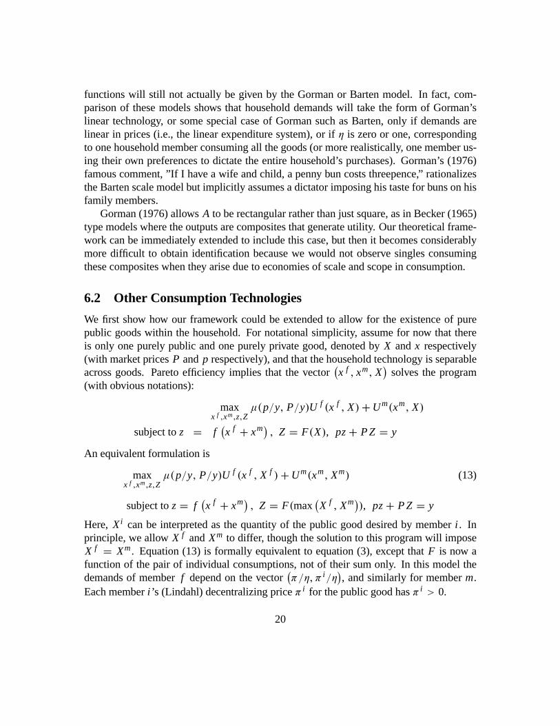
functions will still not actually be given by the Gorman or Barten model. In fact, com-parison of these models shows that household demands will take the form of Gorman’slinear technology, or some special case of Gorman such as Barten, only if demands arelinear in prices (i.e., the linear expenditure system), or if η is zero or one, correspondingto one household member consuming all the goods (or more realistically, one member us-ing their own preferences to dictate the entire household’s purchases). Gorman’s (1976)famous comment, ”If I have a wife and child, a penny bun costs threepence,” rationalizesthe Barten scale model but implicitly assumes a dictator imposing his taste for buns on hisfamily members.

Gorman (1976) allows A to be rectangular rather than just square, as in Becker (1965)type models where the outputs are composites that generate utility. Our theoretical frame-work can be immediately extended to include this case, but then it becomes considerablymore difficult to obtain identification because we would not observe singles consumingthese composites when they arise due to economies of scale and scope in consumption.

6.2 Other Consumption TechnologiesWe first show how our framework could be extended to allow for the existence of purepublic goods within the household. For notational simplicity, assume for now that thereis only one purely public and one purely private good, denoted by X and x respectively(with market prices P and p respectively), and that the household technology is separableacross goods. Pareto efficiency implies that the vector x f , xm, X solves the program(with obvious notations):

maxx f ,xm,z,Z

μ(p/y, P/y)U f (x f , X)+Um(xm, X)

subject to z = f x f + xm , Z = F(X), pz + P Z = y

An equivalent formulation is

maxx f ,xm,z,Z

μ(p/y, P/y)U f (x f , X f )+Um(xm, Xm) (13)

subject to z = f x f + xm , Z = F(max X f , Xm ), pz + P Z = y

Here, Xi can be interpreted as the quantity of the public good desired by member i . Inprinciple, we allow X f and Xm to differ, though the solution to this program will imposeX f = Xm . Equation (13) is formally equivalent to equation (3), except that F is now afunction of the pair of individual consumptions, not of their sum only. In this model thedemands of member f depend on the vector π/η, π i/η , and similarly for member m.Each member i’s (Lindahl) decentralizing price π i for the public good has π i > 0.

20

If the technologies for the public and private goods are both linear, so f (x) = Ax + aand F(X) = BX + b, then the shadow prices satisfy

π = Apy − ap − bP

, π f + πm = B Py − ap − bP

so the sum of individual prices for the public good plays the same role as the price of aprivate commodity. A similar analysis could be used to incorporate externalities within thehousehold, whether positive or negative. Note, however, that with negative externalitiesindividual prices π i for the externality could be negative.

Returning to the general case of n goods, a more general program that encompassesboth models (13) and (3) as special cases is

maxx f ,xm ,z

μ(p/y)U f (x f )+Um(xm) subject to z = F(x f , xm), p z = y (14)

which allows for completely general consumption technology functions F(x f , xm). Likethe other programs, the general household model (14) can be decentralized, but now thecomplete vector of Lindahl shadow prices will be different for members m and f , beingfunctions of the separate derivatives of F (assuming these derivatives exist) with respectto xm and x f . In contrast, our program (3) assumption of an additive technology z =F(x f + xm) makes the derivatives of F with respect to xm and x f equal, resulting inshadow prices π(p/y) that are the same for m and f . The problem with nonadditivetechnology models is that our nonparametric identification result does not hold for them.In particular, it may be the case that several different technology functions F(x f , xm)could generate the same observable demand functions. Identification would then needto rely either on detailed functional form assumptions or on the availability of additionalinformation, such as assignability of goods.

Suppose that our model, which assumes an additive consumption technology z =F x f + xm , were applied to data derived from a more general technology z = F x f , xm .How would this misspecification bias the results? Our additive technology implies thatboth individuals face the same shadow prices π . This will provide a good approximationto a more general technology if agents have similar marginal valuations for the goods, andhence similar shadow prices.

In the particular example of a purely public good, our additive model will provide agood approximation to actual behavior if the household members have a similar willing-ness to pay for the public good. For example, the shadow price of purely public goodshould be one half the market price, leading in the Barten technology πk = Ak pk/y to acoefficient of Ak = 1/2. If additional economies of scale are present, the coefficient maybecome smaller than one half; conversely, diseconomies of scale (or partly private use)would generate Barten coefficients between .5 and 1.

21

6.3 Preference ChangesOur model assumes that the demand functions of household members, h f and hm , areidentified. The simplest way to satisfy this assumption is to assume that individual’s pref-erences for goods do not change when they marry. This does not mean that individualsconsume the same bundles as singles in couples (because the model of a couple permitseconomies of scale and scope in consumption) nor does it rule out individuals gettingutility from marriage, rather, all it implies is that the indifference curves of single menor women living alone are the same as the indifference curves associated with the utilityfunctions Um and U f in the household model. If this assumption holds, then the functionshm and h f can be estimated directly by observing the consumption behavior of single menand single women.

Instead of assuming tastes do not change, we could also attain identification by esti-mating the demand functions for singles, parameterize how those preferences change as aresult of marriage, and use couple’s data to estimate these preference change parametersalong with the other features of the household models, that is, the consumption technol-ogy and sharing rule. For example, suppose that the utility function of individual i livingalone is ordinally represented by Ui(L−1zi ) for some matrix L . We could write this moregenerally as utility given by T Ui(L−1zi), L , where T is monotonic in its first element.The utility function of individual i in the household is ordinally represented by Ui(zi), sothe matrix L embodies the changes in taste for goods that result from marriage. Then thedemand functions for a single i living alone will be

zi = hi(p/yi ) = L−1hi L−1 p/yi

and therefore, given a linear consumption technology, the demand functions of the couple,expressed in terms of the demand functions hi for the members, will be

z = h(p/y) = ALh f L A py − a p

1η(p/y)

+ ALhm L A py − a p

11− η(p/y) + a (15)

In particular, if A and L are diagonal and a = 0, so both the technology and preferencechange have a Barten form, then for each good k, Ak is a technological economies ofscale parameter that should lie between 1/2 and 1 (assuming no diseconomies of scale),while Lk captures common taste changes over the private good equivalent xk = (zk/Ak).If Lk = 1 then tastes for good k do not change with marriage. If Lk > 1 then marriedindividuals like good k less than when they are single.

In this example, taste changes and economies of scale affect couple’s demands in ex-actly the same way. If we had estimated the model assuming no taste change, we would

22

obtain Barten technology estimates of Lk Ak instead of just Ak , and so would end upattributing taste changes to economies of scale. Additional information would then be re-quired to separately identify L and A. For example, any good k that is known to be purelyprivate would have Ak = 1, so an estimated Barten scale other than one for that goodwould equal Lk . Similarly, the estimated Barten scale for any good k that is known tohave Lk = 1 (no taste change) would equal Ak . Any good k that is assignable (meaningthat xk is directly observed) would allow direct estimation of hi

k , which could then be usedin the household’s model to estimate some or all of the parameters of A and compared tothe singles demand functions hi

k to estimate some or all of the taste change parameters L.All prices appear in the demand functions for each good, so it may be possible to identifymany of the technology and taste change parameters from observations of hi

k and hik for a

small number of goods k that are private or assignable or do not undergo a change in tasteupon marriage.

In our empirical application we estimate a Barten technology and apply the model withtwo different interpretations of the result. One is to assume no taste change, interpretingthe estimated parameters as equalling each Ak . We also apply the model assuming theestimated Barten parameters equal Lk Ak , where Lk = 1 if Ak is less than one, otherwisewe assume Ak = 1 and the estimated parameter corresponds to taste change Lk . We alsoexperiment with exploiting assignability of clothing.

In our indifference scale and other welfare calculations, we do not attempt to com-pensate for taste changes, since that, like traditional adult equivalence scales, would re-quire untestable cardinalization assumptions, e.g., equivalence scales based on equatingUi (L−1xi) to Ui(xi) would differ from equivalence scales based on equating the observa-tionally equivalent representations of preferences T Ui(L−1zi), L to T Ui(zi ), I formonotonic transformations T . This is precisely the problem we avoid with our indifferencescale calculations, i.e., this problem does not arise for technology parameters A instead ofL, because preferences do not depend upon A. As a result, using our indifference scales,compensation is purely for resources one received as a household member, and the loss ofeconomies of scale and scope in consumption. We believe this more closely matches theusual notion of maintaining a standard of living than any attempt to also compensate forchanges in tastes.

Note that separating L from A will not be important if the dollar effect of a change intastes for goods is small, implying that Lk is close to one for most goods. For example,joint consumption of heating is likely to have a much larger effect on measured cost sav-ings of living together than on any change in tastes for heat. Separating L from A is largelyirrelevant for some relevant calculations such as demand elasticities, or the interpretationof the sharing rule η as a measure of bargaining power.

In our empirical application we also considered other models of taste change, such

23

as allowing some of the intercept parameters αi to differ for singles living alone versusthose in couples, but attempts to estimate such models were abandoned when the resultingmodels, which are identified through functional form, failed to converge numerically.

6.4 ExternalitiesThe analysis of positive externalities within a household is similar to that of jointly con-sumed goods, while negative externalities affect shadow prices in the opposite direction.Suppose, e.g., that a commodity consumed by one member has a negative impact on theother person. Since the second person’s marginal willingness to pay is negative, the firstperson’s individual shadow price must exceed the household price. In the absence ofeconomies of scale or scope for this commodity, the estimated shadow price would belarger than the market price, leading to a Barten coefficient greater than one. More gen-erally, if a commodity (say, tobacco) is consumed by both members and each individual’sconsumption has a negative impact on the other person’s welfare, then each individualprice may exceed the household price (because at the optimum each member will have apositive marginal willingness to pay to get rid of the other person’s consumption). Over-all, in the absence of preference changes, an estimated Barten coefficient larger than onewould be suggestive of the presence of negative consumption externalities for the com-modity under consideration.

The differences between externalities versus changes in preferences would be hard ifnot impossible to distinguish empirically. For example, if we found that married couplesconsume proportionally more restaurant meals than either single men or single women,this could be due either to externalities (each member’s marginal utility of restaurant din-ing might be enhanced by the presence of their spouse) or by a simple change in pref-erences (members liking restaurant dining better when married). The two explanationshave different implications, e.g., under the externality story only dinners taken with one’sspouse are increased in value, in contrast to the preference change explanation. In practice,available data would hardly allow the estimation of such subtle distinctions.

7 Empirical Application

7.1 DataWe use Canadian FAMEX data from 1974, 1978, 1982, 1984, 1986, 1990 and 1992 on an-nual expenditures, incomes, labour supply and demographics for individual (‘economic’)households. Prices are taken from Statistics Canada. Composite commodity prices areconstructed as the weighted geometric mean of the component prices with budget shares

24

averaged across the strata (couples, single males and single females) for weights. The(non-durable) goods we model are: food at home, restaurant expenditures, clothing, vices(alcohol and tobacco), transport, services and recreation.

We sample single females, single males and couples with no one else present in thehousehold, with women and men aged less than or equal to 42 and 45, respectively. Allagents are in full year full time employment with non-negative net and gross incomes andall couples own a car (to avoid modeling the demand patterns of the 5% of couples in theoriginal sample that did not own cars). Table 1 presents summary statistics for our data.

7.2 Singles Budget SharesOur model starts with a utility derived functional form for the budget shares of singles.For this we use the QUAIDS model described in equations (7), (8), (9), and (10), withi = m for single men and f for single women. We also estimate a QUAIDS for couplesto provide an initial comparison with singles and with our collective household model.

We allow the α and β parameters in the QUAIDS to depend on demographics. Specif-ically we take:

αik = αi

k0 +Mα

m=1αi

kmdm (16)

β ik = β i

k0 +Mβ

m=1β i

kmdm (17)

where Mβ = 2 for singles (dummies for owning a car and being a home owner) andMβ = 1 for couples (a home owner dummy). For the intercept demographics we haveMα = 18 for couples and Mα = 13 for singles. These demographics include four regionaldummies; a house ownership dummy and a dummy for living in a city. For singles wealso have a car ownership dummy. As well we include individual specific demographics:age and age squared, a dummy for having more than high school education, dummies forbeing French speaking or neither English nor French speaking and an occupation dummyfor being in a white collar job. Although these demographics are highly correlated withincouples we need to include both sets so that we can allow for the dependence of couples’budget shares on both sets of individual characteristics. We have 24 and 28 parameters pergood/equation for singles and couples respectively.

As a preliminary analysis we estimate separate QUAIDS models for single men, singlewomen, and couples. We estimate by GMM and take account of the endogeneity of totalexpenditure by using as instruments for singles: all of the demographics and log relativeprices (the included variables) plus log real net income (defined as the log of nominal net

25

Single Single Couplesfemales males Husband Wife

Sample size 1393 1574 1610Net income* 26, 137 30, 890 56, 578

Total expenditure* 11, 855 13, 645 23, 175Wife’s share of gross income - - 0.43

bs(food at home) 0.18 0.16 0.18bs(restaurant) 0.11 0.15 0.11bs(clothing) 0.16 0.09 0.14

bs(vices) 0.07 0.12 0.08bs(transport) 0.21 0.25 0.25bs(services) 0.17 0.10 0.12

bs(recreation) 0.11 0.13 0.11car 0.64 0.78 1

home owner 0.13 0.23 0.58city dweller 0.85 0.81 0.83

age 29.9 31.1 30.2 28.2higher education 0.20 0.25 0.21 0.19

Francophone 0.19 0.17 0.21 0.18Allophone 0.08 0.08 0.08 0.07

White collar 0.43 0.40 0.39 0.37Notes. * mean for 1992 (when prices are unity).

Table 1: Descriptive statistics

26

income divided by a Stone price index computed for our seven non-durables goods) andits square, the product of real net income with the car and home ownership dummies andabsolute log prices. For instruments for couples we use the instruments used for singles(without, of course, the car dummy variables), with individual specific values for husbandsand wives, where appropriate. We also include logs of the individual gross incomes and theratio of the wife’s gross income to total gross income (we discuss these variables below).

The singles models are used for first stage GMM estimates in our joint model, sinceby themselves they are consistent but inefficient in the context of our joint model. TheQUAIDS model for couples, which we only estimate for comparison, is a unitary model,while our actual proposed model is a collective model, essentially a mixture of the twosingle’s QUAIDS models.

To illustrate the differences in demands of single men, single women, and couples,Figure 1 present fitted demand (Engel curve) plots for our seven goods, calculated foragents at the mean level of demographic variables, who live in Ontario in 1992 (the yearand region for which prices are set to unity), with total expenditures ranging from the firstthe ninth decile. We shift the plots for couples to the left in these figures to make themcomparable to the singles plots. We find that food at home is a necessity for all and thattransport and services are necessities for singles. Restaurants and recreation are luxuriesfor all and vices are a luxury for singles. Clothing is a necessity for low income singlemen but a luxury for high income single men (the QUAIDS quadratic term is significant).Vices are a necessity and transport is a luxury for low income couples. In both Table 1and in these figures, the demands of couples more closely resemble the demands of singlewomen than those of single men. The question now is whether our model of a couple as acombination of two singles can capture these effects.

7.3 The Joint ModelFor our empirical application, we assume singles demands have the integrable QUAIDSfunctional form described in equations (7), (8), (9), (10), (16) and (17). The joint modeltherefore includes one set of αi , βi , iand λi parameters (including demographic compo-nents) for men, i = m, and another complete set of these parameters for women, i = f .Let w f

k = ωfk (p/y

f ) and wmk = ωm

k (p/ym) denote the QUAIDS budget share of con-

sumption of good k for single women and single men, respectively.For couples we assume a Barten type technology function defined as

zk = Akxk (18)

for each good k, and so is equivalent to the general linear technology z = Ax + a whenthe matrix A is diagonal and overheads a are zero. The shadow prices for this technology

27

areπk = Ak pk

y(19)

where the couple faces prices p and has total expenditure level y. This technology functionis particularly convenient for budget share models. Let wk = ωk(p/y) be the budgetshare of good k for the household, so ωk(p/y) = pkhk(p/y)/y. With the technologyfunction (18) and corresponding shadow prices (19), equation (6) yields the followingsimple expression for the couple’s budget shares

ωk (p/y) = ηω fkπ

η+ (1− η)ωm

kπ

1− η (20)

Equation (20) shows that, with a Barten type technology, the budget shares of the coupleequal a weighted average of the budget shares of its members, with weights given by theincome sharing rule η and 1−η. Equation (20) shows that η represents both the fraction ofresources controlled by the wife and the extent to which the household’s demands resembleher demands, evaluated at shadow prices.

The parameters of the couples model consist of all the QUAIDS parameters of boththe single’s models ω f and ωm , the Barten scales Ak which we model as constants, andthe parameters of the sharing rule η. Our model for η is

η = exp s δ1+ exp (s δ)

(21)

where s is a household specific vector of distribution factors and δ is a vector of para-meters. This logistic form bounds the sharing rule between zero and one. Based in parton the bargaining models of Browning, Bourguignon, Chiappori and Lechene (1994) andBrowning and Chiappori (1998), the distribution factors that comprise s are a constant,the wife’s share in total gross income, the difference in age between husband and wife, ahome-ownership dummy and log deflated (by a Stone price index) household total expen-diture.

The joint system consists of the vectors of budget shares for singles ω f (p/y f ) andωm(p/ym) and the vector of budget shares for couples ω(p/y). For efficiency these areall estimated simultaneously, since all the parameters in the singles models also appear inthe couples model.

We estimate the joint system by GMM. We assume that the error terms are uncorre-lated across households but are correlated across goods within households. Let ωh be the(n − 1) vector of budget shares for the first n−1 goods consumed by household h. Denotethe vector of all parameter values by θ and let ωh (θ) be the predicted budget shares for

28

household h. The error vector for household h is thus given by uh (θ) = ωh − ωh (θ).Let the numbers of couples, single females and single males be given by Hc, H f and Hmrespectively. Denote the (1× gc) vector of instruments for couples by zc

h and similarly forsingles (where gc = 32 and g f = gm = 25). The vector of moment conditions for couplesis given by the ((n − 1) gc × 1) vector:

νc (θ) =Hc

h=1uh In−1 ⊗ zc

h

and similarly for singles. Define the weighting matrix

Wc =Hc

h=1In−1 ⊗ zc

h ucuc In−1 ⊗ zch

−1

and similarly for singles. The residuals uc are taken from a first stage GMM with anidentity weighting matrix. For the singles these first stage residuals are from the QUAIDSestimates reported earlier. For couples, these first stage residuals are from estimates ofthe couples budget share system (20), estimated using just couples data. Without singlesdata, the parameters from the couples model by itself are not all identified, but all that isrequired for the first stage are unrestricted residual estimates. The GMM criterion is then

minθ

νc (θ) Wcc ν

c (θ)+ ν f (θ) W f νf (θ)+ νm (θ) Wmν

m (θ)

where θ is the full parameter vector. In our system we have at least 258 preference para-meters (6 ∗ 24 − 15 = 129 symmetry constrained QUAIDS parameters for each of menand women, plus the sharing rule and Barten scale parameters). We have 492 instruments(for each good there are 25 instruments for each single strata and 32 for couples), giving amaximum degrees of freedom of 234 for the simplest model.

7.4 Parameter Estimates and AnalysisFor large, highly non-linear systems such as ours, we caution that conventional limitingdistribution measures of standard errors can often be quite misleading; see e.g., Gregoryand Veall (1985). For our preferred specification we found ten distinct local minima, eachof which required a few days of iterations to converge, so our ability to experiment withalternative specifications was limited.

Table 2 present estimates of our model and of two simpler specifications. As a bench-mark, model 1 has no consumption technology function and equal sharing (η = 0.5 and

29

Model1 2 3

Sharing rule 0.5 0.68 0.70∗Barten scale, food 1 0.93 0.82Barten scale, rest 1 0.78 0.79Barten scale, cloth 1 1.70 1.88Barten scale, vices 1 3.19 3.00Barten scale, trans 1 0.55 0.51Barten scale, serv 1 0.59 0.59Barten scale, recr 1 1.31 1.38df 234 226 222χ2 432.0 236.1 224.1P-value (%) 0 30.8 44.8∗ at mean of sharing of factors

Table 2: Results

Ak = 1 for all k), and is decisively rejected. Model 2 specifies the sharing rule and Bartenparameters (η, A1, ...A7) as constants, and improves the fit dramatically; the χ2 (8) statis-tic for these parameters versus model 1 is 195.9, and this model gives a satisfactory valuefor the test of the over-identifying restrictions. Model 3, our preferred model, replaces theconstant sharing rule in model 2 with the model of equation (21) which includes the fourhousehold specific distribution factors described earlier. The χ2 (4) statistic for the inclu-sion of these demographic factors is 12.0, so they are are jointly significant. We shall takethis variant as our preferred specification. Attempts to add fixed costs a to the consumptiontechnology and other extensions were not successful.

Our preferred model imposes strong restrictions on the differences between budgetshares of singles and couples. In figure 2 we present the Engel curve fits for our modelbased on the same reference groups as in figure 1. Our model has far fewer parametersthan the separate unconstrained QUAIDS models in figure 1 (411 versus 270), so thefact that our model generates quite similar estimates is reassuring. The main differencesbetween the two are the couples Engel curves for vices (though the fits for this good wererather imprecise), transport, and perhaps food. Non-nested hypothesis tests we performedcomparing the two models were inconclusive, which is not surprising given the size andcomplexity of the models.

30

Household characteristics Wife’s share ηBenchmark 0.65First quartile total expenditure 0.60Third quartile total expenditure 0.68Renters 0.77Wife’s income share = 0.25 0.65Wife’s income share = 0.75 0.66Husband ten years older 0.65Wife ten years older 0.65

Table 3: Sharing rule implications

7.4.1 The sharing rule

Table 3 gives the values of the sharing rule η for different sets of characteristics. Thebenchmark household has a home-owning husband and wife with the same gross incomeand age and with median total expenditure for Ontario in 1992. Table 3 presents theestimates of the level and variations in the sharing rule.

At our benchmark value the wife’s share is 0.65. If this was purely for private goodsthen this would be implausibly high but it also reflects the effects of joint or public con-sumption. Essentially, this number says that household demand functions look more likewomen’s demand functions than men’s demand functions.

From rows 2 and 3 we see that the wife’s share is strongly increasing in total expen-diture so that in poorer households the wife’s share is much lower. This impact of totalexpenditures on the sharing rule means that household’s demands are not unitary, that is,they are not equal to demands that would arise from the maximization of a single, ordinaryutility function.

Other rows of this table show that the home-ownership status variable has a very strongimpact with renting households apparently having a much higher share for the wife. Aswe saw above, the pattern of home ownership between singles and couples is very differ-ent so this result is probably due at least in part to a selection effect rather than a genuinedifference in intra-household allocations. Neither the wife’s share of income nor their rel-ative ages has much impact on the sharing rule. This is very different from the resultsreported in Browning, Bourguignon, Chiappori and Lechene (1994), which examines con-ventional sharing rules for private goods using similar data on couples. Note that the latterpaper did not include the home ownership dummy in the sharing rule and included realhousehold income instead of total expenditures. Nonetheless the qualitative differencesare striking and suggest that allowing for household technology may have a major impact

31

on our conclusions regarding intrahousehold allocations.

7.4.2 Assignability of Clothing

We do not model men’s and women’s clothing as assignable, showing that our methodol-ogy works without any assignability. However, we do observe men’s and women’s cloth-ing as separate expenditure categories in the data, so assuming clothing is purely privateand that women never use men’s clothing or vice versa, then clothing is assignable in ourdata.

One way to use privateness and assignability of clothing is to generate an (inefficient)alternative estimate of the sharing rule, as the value of η that equates relative clothingshares observed within couples to estimates of clothing shares within the couple based onclothing demand functions estimated from singles data. This simple estimator for η alsoassumes no taste change for clothing after marriage. At base prices this yields an estimateof η of 0.55, somewhat lower than our full model estimates, but still implying that the wifecontrols the majority of household resources.

We also reestimated our entire model treating men’s and women’s clothing as separate,assignable goods in the couple’s model. We do not report these estimates to save space,since relative to Table 2, the results showed no gains in plausibility or precision resultingfrom imposing the additional assignability assumption.

7.4.3 Barten scales and Economies of scale

We now consider estimates of the private good equivalent consumption for married menand married women and the resulting economies of scale. Given estimates of the budgetshare systems for singles, wi

k = ωik(p/y

i ), and for households (equation 20), the privategood equivalent quantities for each household member are given by x f

k = ηω fk (π/η) /πk

and xmk = (1 − η)ωm

k (π/(1− η)) /πk . Define R, the relative economies of scale toconsumption, as

R = p (x f + xm)

y− 1 = p (x f + xm − z)

p zIn Table 4 we present estimates of R and of member’s private good equivalent budget

shares, given η = .5 (equal sharing), and for the median benchmark estimate η = .65.We also present results using estimated Barten scales and Barten scales capped at one.This latter case assumes each estimated Barten scale equals Lk Ak instead of just Ak , asdescribed in the section on preference changes. The results that impose Ak ≤ 1 in Ta-ble 4 (models B and D) assume for example that the estimated scale of 3.0 for vices (see

32

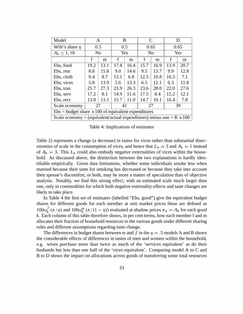
Model A B C DWife’s share η 0.5 0.5 0.65 0.65Ak ≤ 1,∀k No Yes No Yes

f m f m f m f mEbs, food 19.2 13.1 17.8 16.4 15.7 16.9 13.9 20.7Ebs, rest 8.8 15.8 9.0 14.6 9.5 13.7 9.9 12.8Ebs, cloth 9.4 8.7 13.1 6.8 12.5 10.8 16.3 7.1Ebs, vices 5.8 13.9 5.6 13.3 6.5 12.1 6.3 11.8Ebs, tran 25.7 27.3 23.9 26.3 23.6 28.0 22.0 27.6Ebs, serv 17.2 8.1 14.9 11.6 17.5 8.4 15.2 12.1Ebs, recr 13.8 13.1 15.7 11.0 14.7 10.1 16.4 7.8Scale economy 27 41 27 39Ebs = budget share ×100 of equivalent expendituresScale economy = (equivalent/actual expenditures) minus one = R×100

Table 4: Implications of estimates

Table 2) represents a change (a decrease) in tastes for vices rather than substantial disec-onomies of scale in the consumption of vices, and hence that Lk = 3 and Ak = 1 insteadof Ak = 3. This Lk could also embody negative externalities of vices within the house-hold. As discussed above, the distinction between the two explanations is hardly iden-tifiable empirically. Given data limitations, whether some individuals smoke less whenmarried because their taste for smoking has decreased or because they take into accounttheir spouse’s discomfort, or both, may be more a matter of speculation than of objectiveanalysis. Notably, we find this strong effect, with an estimated scale much larger thanone, only in commodities for which both negative externality effects and taste changes arelikely to take place.

In Table 4 the first set of estimates (labelled “Ebs, good”) give the equivalent budgetshares for different goods for each member at unit market prices these are defined as100ω f

k (π/η) and 100ωmk (π/(1− η)) evaluated at shadow prices πk = Ak for each good

k. Each column of this table therefore shows, in per cent terms, how each member f and mallocates their fraction of household resources to the various goods under different sharingrules and different assumptions regarding taste change.

The differences in budget shares between m and f in the η = .5 models A and B showsthe considerable effects of differences in tastes of men and women within the household,e.g. wives purchase more than twice as much of the ‘services equivalent’ as do theirhusbands but less than one half of the ‘vices equivalent’. Comparing model A to C andB to D shows the impact on allocations across goods of transferring some total resources

33

from husbands to wives. The difference between models A and B, like the differencesbetween C and D, is that B and D rule out diseconomies of scale in clothing, vices, andrecreation (see Table 2), attributing the Barten scales that are greater than one to tastechange. This implies lower shadow prices for these goods, with consequent own price,cross price, and income effects on the resulting budget shares of each member, and alarger total estimate of household consumption economies of scale.

The overall scale economy measure R times 100 is given in the last row of Table 4. Inmodels A and C the estimate is R = .27, which means that it would cost the couple 27%more to buy the (private equivalent) goods they consumed if there had been no shared orjoint consumption. The models that rule out diseconomies of scale of course imply greatersavings, with R equal 0.39 or 0.41, showing that singles buying bundles x f and xm wouldin total pay about 40% more than the couples expenditures y. Note that both models C andD are based on the same estimates, and so correspond to our benchmark estimates; theydiffer only in how the estimated Barten scales are interpreted.

7.4.4 Welfare comparisons and Indifference scales

The finding that two singles require 27 to 41 percent more total expenditure than a coupleto buy the same equivalent consumption levels x f + xm represents an upper bound on thetotal amount needed if they actually physically lived apart (while maintaining the samepreferences). This is because differences between market prices and household shadowprices mean that singles living alone can more cheaply attain the same indifference curvesthat x f and xm respectively lie on by rebudgeting. That is what our indifference scalesSi(p/y, η) measure.

In Table 5 we present indifference scales and also the (technological) scale economyparameter, for comparison purposes. For example, in model B in this table we have S f +Sm = 1.38, that is, 38% more income in total rather than 41% given by R, the differencebeing the gains each can get by rebudgeting. In model A, which allows for diseconomiesof scale, we get 14% more income required for singles in total compared to the samemodel’s economies of scale measure of 27%, which implies considerable savings fromsingles’ rebudgeting. However, when comparing models A and B recall that model Bassumes taste differences between single and married individuals (the Lk parameters), andthe indifference scales do not compensate for these taste changes.

Along with equal sharing, we choose the more moderate relative clothing based sharingrule estimate of 0.55 rather than 0.65 for this analysis, because at 0.65 we obtain Sm < .5which implies that men are better off single even with less than half of household income.This is the result of two effects: we estimate that married women receive more privategoods and they have more influence on the demand for shared goods. Both effects result in

34

Model A B C DWife’s share η 0.5 0.5 0.55 0.55Ak ≤ 1,∀k No Yes No YesScale economy R × 100 27 41 27 39indiff. scale S f × 100 58 68 63 74indiff. scale Sm × 100 56 70 50 63

Table 5: Adult equivalence scales

generally higher estimated scales for women than for men. Note that individuals could stillchoose to marry when their indifference scale is less than one half, or when it is less thanthe fraction of income or other resources they bring to the marriage, because indifferencescales are only based on indifference curves over goods. Utility from companionship cancompensate for possible material losses.

Our ranges of indifference scales estimates are quite wide, with values between 58%and 74% for women and between 50% or less to 70% for men. Most of this range comesfrom differing interpretations of the estimated Barten scales. Future work on distinguish-ing between taste changes versus sharing and jointness of consumption, and generatingbetter sharing rule estimates would go a long way towards improving the precision of theseestimates. Both would greatly benefit from additional data, particularly direct observationof at least some features of the consumption patterns of individuals within households.

8 ConclusionsWe model households in terms of the utility functions of its members, a bargaining or so-cial welfare function, and a consumption technology function. By employing a collectivemodel and a separate consumption technology, we combine data from singles and cou-ples to identify a version of equivalence scales that we call indifference scales, as wellas consumption economies of scale, individual members’ control of resources within thehousehold, and other related concepts, without assumptions regarding cardinalizations orinterpersonal comparability of preferences. Unlike traditional adult equivalence scalesthat attempt to compare the utility of an individual to that of a household, our indifferencescales directly compare the cost of living for an individual within a household to the costof living of the same individual living alone.

We also provide duality results that facilitate the empirical application of our model.These include the use of indirect utility functions to describe individual household mem-bers’ preferences, an income sharing rule to model the outcome of the household bargain-

35

ing or resource allocation process, and shadow prices that embody economies of scale andscope arising from joint consumption. We demonstrate generic nonparametric identifica-tion of our model.

We empirically apply our model to Canadian consumption data on single men, singlewomen and married couples. Among other empirical results, we find that couples save theequivalent of about one third of their total expenditures through shared and joint consump-tion of goods, that wives on average control between a half and two thirds of householdresources, and that singles need to spend between one half to three fourths as much ascouples to attain the same standard of living by themselves as they attain as members of atwo person household.

Given our framework, one useful area for further work would be the developmentof more detailed alternative identifying assumptions. Without preference changes or ex-ternalities within the household, our model is very much over identified, in fact, in ourQUAIDS specification many of the parameters of the entire consumption technology couldbe separately identified from the couple’s demands for a single good. This overidentifi-cation might be exploited by relaxing the model in ways that incorporate and identifypossible externalities (among individuals within the household) or by allowing for moregeneral models of individual’s preference changes that result from marriage or householdformation in general. Direct observation of some elements of the private good equivalentconsumption vector x would also aid identification, by distinguishing changes in prefer-ences from pure economies of scale or scope in consumption. Example of such data wouldbe direct measures of the quantity of food wasted (discarded) by singles and couples, ormeasures of the fraction of time couples drive together versus alone. Exploiting assignabil-ity of some goods also helps theoretical identification, though we did not find empiricalimprovements from assuming assignability of clothing.

Alternative identifying conditions that minimize reliance on the consumption data ofsingles would also be valuable for extending the model to directly include the utility func-tions of children, which for now must be assumed to be joint with the utility of an adulthousehold member. Another useful direction for future research would be the develop-ment of empirically tractable duality and identification results for more general, nonlinearconsumption technology functions.

The generality of our estimated model in the number of goods and functional forms ofits components resulted in many numerical and convergence difficulties. It would be usefulto investigate simplifications that preserve the main features of the model. For example,the sharing rule can in principle be identified and estimated just from combining data onsingles and couples for a single good.

An interesting extension of our model would be the introduction of time allocation asanother good. In particular, our consumption technology function could directly embody

36

the extent to which couples achieve economies of scale in time use by combining chores(such as one member cooking meals for both), and economies of scope such as saving bothtime and gasoline by commuting together. More generally, the consumption technologyfunction could be merged with home production functions, as in rural households thatgrow crops for personal consumption.

While our particular identifying and functional form assumptions should be open todebate and improvement, we believe that the general model we have provided is an ap-propriate framework for estimating and analyzing adult equivalence scales, consumptioneconomies of scale, household members’ bargaining power, and other concepts relatingto household preferences, consumption, and demand behavior. It could be interesting toextend the model to other aspects of collective decision making, such as household for-mation and dissolution, fertility, the allocation of time, durables consumption and savingsdecisions.

9 Appendix

9.1 Proofs of PropositionsPROOF OF PROPOSITION 1: The Lagrangian for the household’s program can be writ-ten as μ(p/y)U f (x f ) + Um(xm) + λ 1− (p/y) F(x f + xm) which gives first orderconditions

μ(p/y)∂U f (x f )

∂x fk

= λy

n

j=1p j∂F j (x f + xm)

∂x fk

,∂Um(xm)

∂xmk

= λy

n

j=1p j∂F j (xm + xm)

∂xmk

Define π to be the vector of elements πk , k = 1, ..., n and define η by

πk =nj=1 p j/y ∂F j (x)/∂xk

ni=1 xi

nj=1 p j/y ∂F j (x)/∂xi

(22)

η =n

i=1x f

i π i (23)

evaluated at the optimizing values x f = x f (p/y), xm = xm(p/y), and x = x f (p/y) +xm(p/y). By construction 1− η = n

i=1 xmi π i . The above first order conditions can then

37

be rewritten as

μ(p/y)∂U f (x f )

∂x fk

= κπk

∂Um(xm)

∂xmk

= κπk

where κ = (λ/y) ni=1 xi

nj=1 p j∂F j(x)/∂xi . Then

∂U f (x f )/∂x fk

ni=1 x f

i ∂U f (x f )/∂x fi

= πkni=1 x f

i π i= πk

η

∂Um(xm)/∂xmk

ni=1 xm

i ∂Um(xm)/∂xmi

= πkni=1 xm

i π i= πk

1− ηand these are identical to the first order conditions of the programs

maxx f

U f (x f ) subject to π x f = η

maxxm

Um(xm) subject to π xm = 1− η

which define the functions h f and hm .

PROOF OF PROPOSITION 2: From the proof of Proposition 1 we have that a first ordercondition of the household’s program is

μ(p/y)∂U f (x f )

∂x fk

= κπk

The first order condition of member f ’s optimization V f (π/η) = max{U f (x f ) | π x f ≤η} gives ∂U f (x f )/∂x f

k = λ f πk and using the envelope theorem we obtain

μ(p/y)∂V f (π/η)

∂η= λ0.

Apply the same logic to member m gives

∂V m(π/(1− η))∂(1− η) = λ0

The proposition follows from equating these two expression for λ0 and solving forμ(p/y).

38

PROOF OF PROPOSITION 3: Let A jk denote the j, k th element of A and a j denotethe j th element of a. Then Equation (22) with F(x) = Ax + a is

πk =nj=1 p j A jk

ni=1 xi

nj=1 p j A ji

=nj=1 p j A jk

ni=1 xi

nj=1 p j A ji

so π = A p/(p Ax) and p Ax = p A(A−1(z − a)) = p (z − a)) = y − p a. Givenπ , equation (6) the follows from equation (4) with z = A(x f + xm) + a. Having π =A p/ y − a p means that π is not a function of U f , Um or μ, so any changes in thosefunction that change the resulting optimal x f for a given p/y can change η = x f π whileholding π fixed.

PROOF OF PROPOSITION 4: Take a finite set of price vectors p1, ..., pT where T ≥n + 10. These may be interpreted as prices in different time periods. For any pt and anyy, let zt = h(pt/y) denote the corresponding household demands. From Proposition 3 wehave

zt = Ah f A pt

y − a pt1

η(pt/y)+Ahm A pt

y − a pt1

1− η(pt/y)+a, t = 1, ..., T (24)

This provides, for each t , (n − 1) independent equations, hence a total of (n − 1) T equa-tions. The unknowns are the matrix A, the vector a and the scalars ηt = η(pt/y), t =1, ..., T ; hence a total of n2 + n + T unknowns. If n ≥ 3, then with T ≥ n + 10, thenumber of equations exceeds the number of unknowns. This shows that, generically onthe demand functions h f and hm and on the sharing rule η, the equations are linearlyindependent, precisely because of the non linearities introduced by these functions. Iden-tification in this type of model is at best generic;.see, e.g., Chiappori and Ekeland (2004).In our case, for instance, if η is constant and h f and hm are linear, the linear indepen-dence of the equations is no longer guaranteed. With linear independence, the system isgenerically (over) identified. Given identification of A and a,we then have identification ofF(x) = Ax+a and π(p/y) = A p/(y−a p) . The sharing rule η (p/y) is then identifiedfor all p/y from equation (6) and identification of xm and x f follows from equation (4).

PROOF OF PROPOSITION 5: The AIDS quantity demand for good j consumed bymember i is

hij(p/y

i) = yi

p jαi

j + ij ln p + βi

j ln yi − ci (p)

whereci (p) = (ln p) αi + 1

2(ln p) i ln p

39

lnbi (p) = (ln p) βi

αi and βi are n-vectors of parameters, i is an n × n matrix of parameters, e αi = 1,e βi = i e = 0 where e is an n-vector of ones, and i is symmetric.

Linear technology implies that the shadow price for good j is

π j = A· j py − a p

= k Akj pk

y − a p

where A· j is the transpose of the j’th column of A and Akj is the k’th element of A· j .With members having AID demand functions and linear consumption technology, the

couple’s quantity demand for good k is

hk(p/y) =j

Ak j

⎡⎣ ηπ j

αfj + f

j lnπ + β fj ln (η)− c f (π) +

1−ηπ j

αmj + m

j lnπ + βmj ln (1− η)− cm (π)

⎤⎦+ ak

hk(p/y) = y − a pj

Akj

⎡⎢⎢⎢⎣η 1

A· j p αfj + f

j ln Apy−a p + β f

j ln (η)− c f Apy−a p

+ (1− η) 1A· j p

⎛⎝ αmj + m

j ln Apy−a p

+βmj ln (1− η)− cm Ap

y−a p

⎞⎠⎤⎥⎥⎥⎦+ak

Given hk(p/y) for each good k, the constants ak are identified as the intercept terms,and we may identify the summation by hk(p/y)− ak/ y − a p . Now use

ci (π) = ci Apy − a p

= (ln Ap) αi − ln y − a p + 12(ln (Ap)) i ln (Ap)

to write this summation term as

j

A jk

A· j p

⎡⎢⎢⎢⎢⎣η

αfj + f

j ln (Ap)+β

fj ln (η)− (ln Ap) α f − ln y − a p + 1

2(ln (Ap)) f ln (Ap)

+ (1− η) αmj + m

j ln (Ap)+βm

j ln (1− η)− (ln Ap) αm − ln y − a p + 12(ln (Ap)) m ln (Ap)

⎤⎥⎥⎥⎥⎦For each good k, the coefficient of ln y in this expression is

−j

ηβfj + (1− η) βm

j

(A j/Akj )p

40

where the summation is now over all goods j for which Akj is not equal to zero. Variationin y therefore provides identification of the above expression for each good k. Variationof p in the above expression for each k identifies

ηβfj + (1− η) βm

j

A j/Akj

for triplets of goods j, k, having Akj = 0 and A j = 0. The above expression with= k identifies η, since βm

j and β fj are identified from singles, and therefore A j/Akj is

also identified. Define A j = A j/A j j and d j = A j j . Identification of A j/Akj impliesidentification of A j for all j, . What remains is to identify each d j .

The term Akj/A· j p = 1/ (A j/Akj )p is identified for each j , which implies basedon the large summation term above that

η αfj + f

j ln (Ap)+ β fj ln (η)− (ln Ap) α f + 1

2(ln (Ap)) f ln (Ap)

+ (1− η) αmj + m

j ln (Ap)+ βmj ln (1− η)− (ln Ap) αm + 1

2(ln (Ap)) m ln (Ap)

is identified for each good j . The component of this expression that is quadratic in ln (Ap)is

ln (Ap) −ηβ fj12

f − (1− η) βmj

12

m ln (Ap)

=k

lnj

d j Akj p j lnj

d j A j p j ϕk

where ϕk and Akj are already identified for all j, k, . Variation in p in this expressionthen identifies d j , which completes the identification.

Note that the technology and sharing rule are substantially overidentified. Given thedemand functions of members, the couple’s demands for each good k separately identifyη, a (from the y − a p term) and A j/Akj for all j, k, having Akj = 0. Therefore,observing couple’s demands for all goods, not just one, greatly overidentifies these terms.In particular, if the k th row of A has all nonzero elements, then (given the demands ofsingles) the technology and the sharing rule can be completely identified just by observingcouple’s demands for the k th good. In addition to the overidentification resulting fromobserving the couple’s demands for multiple goods, only the terms involving the inter-cept, the coefficient of ln y, and the quadratic in ln (Ap) were used for identification, soall the other terms in the couple’s demands, such as the linear in ln (Ap) term, provideadditional overidentifying restrictions. These various overidentifying assumptions may be

41

used to relax the assumptions regarding unequal and nonzero parameters in the statementof Proposition 5.

Similarly, the above proof applies when single’s have QUAIDS demands, since inthat case the only difference in the model is the addition of more terms (in particular, aquadratic in ln y) which provide more overidentifying restrictions.

9.2 Nonparametric IdentificationWe now show how the generic identification in Proposition 4 extends to the case wherethe consumption technology function F is an unknown smooth function. Let ρ = p/yand let F be the space of increasing C2 functions with range and domain equal to thepositive orthant. Define a mapping T by the following procedure. Given any elementF ∈ F , treat F as if it were the true technology function by defining the correspondingshadow price vector π(ρ) = DF(x) .ρ/ x DF(x) .ρ evaluated at x = F−1h(ρ). Nowlet x(ρ, η) = hmπ(ρ)/(1− η)+ h f π(ρ)/η, and for every ρ in the positive orthant defineη(ρ) by η(ρ) = arg minη∗∈0,1 max|x(ρ, η∗) − F−1h(ρ)|. Finally, define the function Fby F [x(ρ, η(ρ))] = h (ρ). This procedure defines a mapping F = T F .

The true technology function F(x) is a fixed point of this mapping, and the true shar-ing rule η(ρ) equals η(ρ) evaluated using F = F . A sufficient condition to ensure theidentification of η given identification of F is that there exist an element of the vectorx(ρ, η) that is strictly monotonic in η (and a primitive sufficient condition for this is theexistence of a good that is only consumed by one household member, who has a demandfunction for that good that is strictly monotonic in total expenditure).T might not be a contraction mapping, and so may not have a unique fixed point.

However, for suitably regular demand functions (those for which the tangent application toT is Fredholm) each fixed point will be locally unique as a consequence of Smale’s (1973)generalized transversality theorem. This provides local generic identification. Ordinaryregularity conditions such as monotonicity and domain constraints further restrict the setof feasible solution functions.

Global identification results if only one fixed point is present or if, among all fixedpoints, only one satisfies the required regularity conditions. This describes formally whatwe mean by ’generic’ identification. A similar case of generic identification appears inChiappori and Ekeland (1999). Informally, our construction of the mapping T shows thata sufficient number of demand functions are identified to permit recovery of F and η,so these functions will be identified as long as the demand functions are not too simple.For example, as shown earlier, a linear technology is not identified if members’ demandfunctions are also linear (specifically, the linear expenditure system), but are identified fornonlinear member demands like the Almost Ideal or QUAIDS.

42

References[1] BANKS, J., R. BLUNDELL, AND A. LEWBEL, (1997), ”Quadratic Engel Curves and

Consumer Demand,” with James Banks and Richard Blundell, Review of Economicsand Statistics, 79, 527-539.

[2] BARMBY, T. AND N. SMITH, (2001), ”Household labour supply in Britain and Den-mark: some interpretation using a model of Pareto optimal behaviour,” Applied Eco-nomics, 33, 1109-1116.

[3] BARGAIN, O., M. BEBLO, D. BENINGER, R. BLUNDELL, R. CARRASCO, M.-C.CHIURI, F. LAISNEY, V. LECHENE, E. LONGOBARDI, M. MYCK, N. MOREAU,J. RUIZ-CASTILLO, AND F. VERMEULEN (2004), ”Collective models of householdlabour supply with non-convex budget sets and non-participation: a calibration ap-proach,” Review of the Economics of the Household, forthcoming.

[4] BARTEN, A. P. (1964), ”Family Composition, Prices, and Expenditure Patterns,” inEconometric Analysis for National Economic Planning: 16th Symposium ColstonSociety, P. Hart, G. Mills, and J. K. Whitaker, eds., 277-292, London: Butterworth.

[5] BECKER, G. (1965), ”A Theory of the Allocation of Time,” Economic Journal, 75,493-517.

[6] BLACKORBY, C. AND D. DONALDSON (1994), ”Measuring Costs of Children: ATheoretical Framework” in The Measurement of Household Behavior, R. Blundell,I. Preston, and I. Walker, Eds., 70-85, Cambridge: Cambridge University Press

[7] BLUNDELL, R. (1988), ”Consumer Behavior: Theory and Empirical Evidence - ASurvey,” Economic Journal, 98, 16-65.

[8] BLUNDELL, R. AND A. LEWBEL (1991), ”The Information Content of EquivalenceScales,” Journal of Econometrics, 50, 49-68.

[9] BLUNDELL, R, I. PRESTON, AND I. WALKER (EDS) (1994), The Measurement ofHousehold Welfare, Cambridge: Cambridge University Press.

[10] BOURGUIGNON, F. AND P.-A. CHIAPPORI (1994), ”The Collective Approach toHousehold Behavior” in The Measurement of Household Behavior, R. Blundell, I.Preston, and I. Walker, Eds., 70-85, Cambridge: Cambridge University Press

[11] BROWNING, M. (1992), ”Children and Household Economic Behavior,” Journal ofEconomic Literature, 30, 1434-1475.

43

[12] BROWNING, M., F. BOURGUIGNON, P.A. CHIAPPORI, AND V. LECHENE (1994),”Incomes and Outcomes: a Structural Model of Intrahousehold Allocation,” Journalof Political Economy, 102, 1067-1096.

[13] BROWNING, M., AND P.A. CHIAPPORI, (1998), ”Efficient Intra-household Alloca-tions: A General Characterization and Empirical Tests,” Econometrica, 66, 1241-78.

[14] CHESHER, A., (1998) ”Individual Demands from Household Aggregates: Time andAge Variation in the Quality of Diet,” Journal of Applied Econometrics, 13, 505-524.

[15] CHIAPPORI, P.A. AND I. EKELAND (1999), ”Aggregation and Market Demand: AnExterior Differential Calculus Viewpoint,” Econometrica, 67, 1435-1457.

[16] CHIAPPORI, P.A. AND I. EKELAND (2005), ”Characterizing Group Behavior”, un-published manuscript.

[17] CHIAPPORI, P.-A., FORTIN, B. AND G. LACROIX (2002), "Marriage Market, Di-vorce Legislation and Household Labor Supply", Journal of Political Economy, 110,37-72

[18] DEATON, A. AND J. MUELLBAUER, (1980a), Economics and Consumer Behavior,Cambridge: Cambridge University Press.

[19] DUFLO, E. (2000), "Child outcomes in Africa. Child health and household resourcesin South Africa: Evidenced from the old age pension program," American EconomicAssociation Papers and Proceedings, 90, 393-398.

[20] GORMAN, T. (1976), ”Tricks With Utility Functions,” In Essays in Economic Analy-sis: Proceedings of the 1975 AUTE Conference, Sheffield, M. J. Artis and A. R.Nobay, eds., Cambridge: Cambridge University Press.

[21] GREGORY, A. AND M. VEALL (1985), ”Formulating Wald Tests of Nonlinear Re-strictions”, Econometrica, 53, 1465-68.

[22] JORGENSON, D. W. (1997), Welfare Volume 2: Measuring Social Welfare, Cam-bridge, Massachusetts: MIT Press.

[23] LEWBEL, A. (1985), “A Unified Approach to Incorporating Demographic or OtherEffects into Demand Systems,” Review of Economic Studies, 52, 1-18.

[24] LEWBEL, A. (1989), ”Household Equivalence Scales and Welfare Comparisons,”Journal of Public Economics, 39, 377-391.

44

[25] LEWBEL, A. (1997), ”Consumer Demand Systems and Household EquivalenceScales,” Handbook of Applied Econometrics, Volume II: Microeconomics, M. H.Pesaran and P. Schmidt, eds., Oxford: Blackwell Publishers Ltd.

[26] LEWBEL, A., (2003), ”Calculating Compensation in Cases of Wrongful Death,”Journal of Econometrics, 113, 115-128.

[27] LINDAHL, E., (1919), ”Just Taxation - A Positive Solution," in R. Musgave and A.Peacock, eds., Classics in the Theory of Public Finance, London: MacMillan.

[28] MUELLBAUER, J. (1977), ”Testing the Barten Model of Household ConsumptionEffects and the Cost of Children,” Economic Journal, 87, 460-487.

[29] NELSON, J. A. (1988), ”Household Economies of Scale in Consumption: Theoryand Evidence,” .Econometrica, 56 1301-1314.

[30] PENDAKUR, K. (1999), "Estimates and Tests of Base-Independent EquivalenceScales", Journal of Econometrics, 88, 1-40.

[31] POLLAK, R. A. AND T. J. WALES (1979), ”Welfare Comparisons and EquivalenceScales,” American Economic Review, 69, 216-221.

[32] POLLAK, R. A. AND T. J. WALES (1992), Demand System Specification and Esti-mation, Oxford: Oxford University Press.

[33] RUBALCAVA, L., AND D. THOMAS (2000), "Family Bargaining and Welfare",Mimeo RAND, UCLA.

[34] SLESNICK, D. (1998), ”Empirical Approaches to the Measurement of Welfare” Jour-nal of Economic Literature, 36, 2108-2165.

[35] SMALE, S. (1973), "An infinite dimensional version of Sard’s theorem," AmericanJournal of Mathematics, 87, 213-221.

[36] THOMAS, D. (1990), “Intra-Household Resource Allocation: An Inferential Ap-proach”, Journal of Human Resources, 25, 635-664.

[37] THOMAS D, CONTRERAS D, FRANKENBERG E. (1997), "Distribution of PowerWithin the Household and Child Health." Santa Monica, CA: RAND.

[38] VERMEULEN, F. (2000), ”Collective Household Models: Principles and Main Re-sults,” Center for Economic Studies, University Leuven, Discussion Paper.

45

Figure 1: QAIDS �ts for singles and couples.

45

Figure 2: Model �ts for singles and couples.

46