Estimating CH , CO and CO emissions from coal mining and ...

Atmos. Chem. Phys., 20, 12675–12695, 2020https://doi.org/10.5194/acp-20-12675-2020© Author(s) 2020. This work is distributed underthe Creative Commons Attribution 4.0 License.

Estimating CH4, CO2 and CO emissions from coal mining andindustrial activities in the Upper Silesian Coal Basin using anaircraft-based mass balance approachAlina Fiehn1, Julian Kostinek1, Maximilian Eckl1, Theresa Klausner1, Michał Gałkowski2,3, Jinxuan Chen2,Christoph Gerbig2, Thomas Röckmann4, Hossein Maazallahi4, Martina Schmidt5, Piotr Korben5, Jarosław Neçki3,Pawel Jagoda3, Norman Wildmann1, Christian Mallaun6, Rostyslav Bun7,8, Anna-Leah Nickl1, Patrick Jöckel1,Andreas Fix1, and Anke Roiger1

1Deutsches Zentrum für Luft- und Raumfahrt (DLR), Institut für Physik der Atmosphäre, Oberpfaffenhofen, Germany2Max-Planck-Institut für Biogeochemie (MPI-BGC), Jena, Germany3Faculty of Physics and Applied Computer Science, AGH University of Science and Technology, Cracow, Poland4Institute for Marine and Atmospheric research Utrecht, Utrecht University, Utrecht, the Netherlands5Institute of Environmental Physics, University of Heidelberg, Heidelberg, Germany6Deutsches Zentrum für Luft- und Raumfahrt (DLR), Flugexperimente, Oberpfaffenhofen, Germany7Department of Applied Mathematics, Lviv Polytechnic National University, Lviv, Ukraine8Faculty of Applied Sciences, WSB University, Dabrowa Górnicza, Poland

Correspondence: Alina Fiehn ([email protected])

Received: 25 March 2020 – Discussion started: 18 May 2020Revised: 24 August 2020 – Accepted: 7 September 2020 – Published: 3 November 2020

Abstract. A severe reduction of greenhouse gas emissionsis necessary to reach the objectives of the Paris Agreement.The implementation and continuous evaluation of mitiga-tion measures requires regular independent information onemissions of the two main anthropogenic greenhouse gases,carbon dioxide (CO2) and methane (CH4). Our aim is toemploy an observation-based method to determine regional-scale greenhouse gas emission estimates with high accuracy.We use aircraft- and ground-based in situ observations ofCH4, CO2, carbon monoxide (CO), and wind speed from tworesearch flights over the Upper Silesian Coal Basin (USCB),Poland, in summer 2018. The flights were performed as a partof the Carbon Dioxide and Methane (CoMet) mission abovethis European CH4 emission hot-spot region. A kriging algo-rithm interpolates the observed concentrations between thedownwind transects of the trace gas plume, and then the massflux through this plane is calculated. Finally, statistic and sys-tematic uncertainties are calculated from measurement un-certainties and through several sensitivity tests, respectively.

For the two selected flights, the in-situ-derived annual CH4emission estimates are 13.8±4.3 and 15.1±4.0 kg s−1, which

are well within the range of emission inventories. The re-gional emission estimates of CO2, which were determinedto be 1.21± 0.75 and 1.12± 0.38 t s−1, are in the lowerrange of emission inventories. CO mass balance emissionsof 10.1±3.6 and 10.7±4.4 kg s−1 for the USCB are slightlyhigher than the emission inventory values. The CH4 emissionestimate has a relative error of 26 %–31 %, the CO2 estimateof 37 %–62 %, and the CO estimate of 36 %–41 %. These er-rors mainly result from the uncertainty of atmospheric back-ground mole fractions and the changing planetary boundarylayer height during the morning flight. In the case of CO2,biospheric fluxes also add to the uncertainty and hamperthe assessment of emission inventories. These emission es-timates characterize the USCB and help to verify emissioninventories and develop climate mitigation strategies.

Published by Copernicus Publications on behalf of the European Geosciences Union.

12676 A. Fiehn et al.: Estimating CH4, CO2 and CO emissions from coal mining

1 Introduction

One of the main objectives of the Paris Agreement is to keepthe global temperature rise well below 2 ◦C compared to pre-industrial levels (UNFCCC, 2015). This ambitious goal canonly be reached by a severe reduction of greenhouse gasemissions. The development of efficient mitigation strategiesand the implementation and management of long-term poli-cies requires consistent, reliable, and timely information onemissions of the two main anthropogenic greenhouse gases,carbon dioxide (CO2) and methane (CH4). Carbon monox-ide (CO) can be used as an additional tracer for comparisonwith emission inventories and as a proxy for CO2 from fossilfuel combustion. It is produced from the incomplete combus-tion of fossil fuels and biomass and reacts with the hydroxylradical (OH), thus affecting the main sink of CH4.

The globally averaged atmospheric abundances of CO2and CH4 have increased by 47 % to 407.8± 0.1 ppm and by159 % to 1869±2 ppb, respectively, in the period from 1750to 2018 (WMO, 2019). The relative contribution of individ-ual sources and sinks to atmospheric CH4 is still highly un-certain and the factors that affect these sources and sinks arenot fully understood (Saunois et al., 2020). After a period ofstable mole fractions since 2000, the atmospheric abundanceof CH4 has started to increase again in 2007, and after 2014the increase intensified yet again (Nisbet et al., 2014, 2016).The reason for this increased growth is currently investigatedin several studies, which partly contradict each other by dis-cussing biogenic sources, fossil fuel emissions and/or a de-crease in the OH sink (Hausmann et al., 2016; Schaefer et al.,2016; Saunois et al., 2017; Turner et al., 2017; Worden et al.,2017; Nisbet et al., 2019).

Atmospheric emission inventories for trace species areusually based on bottom-up data-based approaches. Here,emissions for individual facilities, sectors, or sources arecompiled into a comprehensive database. If direct emissiondata are not available, they are often calculated using activ-ity data, like the mass of coal extracted, together with emis-sion factors. For Annex I countries, sector-specific emissionsof greenhouse gases have to be reported annually under theUnited Nations Framework Convention on Climate Change(UNFCC). Other countries are encouraged to report nationaltotals of emissions. Bottom-up inventories can thus includesingle-source emissions or national totals, or they can be dis-aggregated on different spatial scales. These gridded emis-sion inventories commonly use national emission totals anddistribute them across each country using proxy data likepopulation density or single facility locations. This methodis used to compile emission inventories, which are used inclimate projections, for example. The neglect of regional dif-ferences and the uncertainties in the proxy data and emis-sion factors introduce high uncertainties into the emission in-ventories at grid cell level (Janssens-Maenhout et al., 2019).Without accurate emission estimates it is challenging to cre-

ate reliable future climate projections and develop efficientmitigation strategies.

Therefore, there is a strong need for an independent andobjective verification of emissions from individual sourcesor source regions based on atmospheric observations, usu-ally referred to as top-down approaches. Top-down studiesbased on satellite data provide information on global and re-gional scales. For methane, emission quantification of indi-vidual sources has recently been demonstrated on very largepoint sources (Pandey et al., 2019; Varon et al., 2019), butquantification of smaller sources is still difficult. Here, air-borne measurements reveal more detailed insights on smallerscales, because in situ measurements allow the study of emis-sion sources with high spatial resolution and accuracy. High-precision measurements of atmospheric concentration can beused for the top-down estimation of emissions from specificregions or sectors using atmospheric inversion models (Gur-ney et al., 2002; Thompson et al., 2014; Bergamaschi et al.,2018) and for the validation of numerical models used to cal-culate atmospheric abundances based on bottom-up emissioninventories (Krinner et al., 2005; O’Shea et al., 2014). Air-borne measurements provide highly valuable data for an in-dependent assessment of anthropogenic CH4, CO2 and COemissions, because the majority of these emissions originatefrom a small fraction of the globe, namely fossil fuel ex-ploitation facilities, cities and power plants. Airborne mea-surements have shown to be useful in emission assessmentof anthropogenic emissions from several sectors, includinglandfills (Cambaliza, 2015; Krautwurst et al., 2017) and oiland gas production regions (Karion et al., 2015; Yuan et al.,2015; Alvarez et al., 2018; Barkley et al., 2019). Plant etal. (2019) and Ren et al. (2018) showed that North Americancities emit more CH4 than suspected, because of underesti-mation of natural gas leakage or lack of inclusion of end useemissions.

Aircraft top-down approaches can be used in several waysto obtain greenhouse gas flux estimates. One way is the massbalance approach, where the emissions are estimated fromobserved in situ mole fractions and wind speeds in the tar-get region. Different flight patterns are used for mass balancestudies: a single downwind flight transect in the approximatevertical center of the boundary layer (Karion et al., 2013) orseveral transects of the plume at the same height but differ-ent distances from the source (Turnbull et al., 2011) are suf-ficient in the case of a well-mixed planetary boundary layer(PBL). A better understanding of vertical trace gas distribu-tion is achieved by several transects at different heights butthe same distance (Cambaliza, 2015; Karion et al., 2015; Pittet al., 2019). Single point sources or small areas can be as-sessed by circular flight paths at different heights (Conley etal., 2017; Tadic et al., 2017; Ryoo et al., 2019). The airborneeddy covariance technique can directly infer vertical fluxes(Hiller et al., 2014; Yuan et al., 2015). Further techniques forairborne emission estimation include active and passive re-mote sensing instruments (Amediek et al., 2017; Krautwurst

Atmos. Chem. Phys., 20, 12675–12695, 2020 https://doi.org/10.5194/acp-20-12675-2020

A. Fiehn et al.: Estimating CH4, CO2 and CO emissions from coal mining 12677

et al., 2017). All methods can be combined with inverse mod-eling to derive emission distributions (Kort et al., 2008; Pol-son et al., 2011; Brioude et al., 2013; Xiang et al., 2013; Cuiet al., 2015).

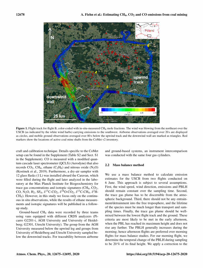
This study is part of the Carbon Dioxide and Methane(CoMet) mission. The goal of CoMet is to develop and eval-uate methods for the independent monitoring of greenhousegas emissions and to provide data for satellite validation.CoMet combined a suite of airborne active (lidar) and pas-sive (spectrometers) remote sensors with in situ instrumentsto provide local- to regional-scale data about atmosphericconcentrations of CO2 and CH4 and to derive emissions ondifferent spatial scales. One of the foci of CoMet was the Up-per Silesian Coal Basin (USCB), located in southern Poland,which represents one of the largest European CH4 emis-sion sources with a total of around 500 kt CH4 a−1 (∼ 3 %of European CH4 emissions), emitted from about 40 hardcoal mines (EEA, 2020). CH4 is released from the coal de-posits and bedrock before and during mining and ventilatedto the atmosphere through individual ventilation shafts dueto safety reasons (Fig. 1). The USCB is also a heavily in-dustrialized urban agglomeration of >2 million inhabitants.During the CoMet mission in early summer 2018, we per-formed airborne in situ measurements of CH4, CO2 and COaboard the DLR aircraft Cessna Grand Caravan 208B.

During 10 research flights conducted in May andJune 2018, we studied emissions from coal mine ventila-tion shafts, power plants and other industrial facilities inthe USCB region by using an airborne mass balance ap-proach. Depending on the wind situation, different areas ofthe USCB region were targeted. To account for the lower partof the emission plume not accessible by aircraft, a number ofvans equipped with mobile in situ measurement systems con-ducted ground-based measurements in a coordinated manner.Here we present trace gas observations from the two massbalance flights targeting the emissions of the entire USCB,one in the morning and one in the afternoon of the same day,6 June 2018. In Sect. 2 we present the observational data usedin this study to derive emission estimates, a theoretical de-scription of the mass balance method including the statisticalinterpolation method kriging together with the uncertaintyanalysis and an overview of emission inventories availablefor the USCB. Section 3 contains the results of the mass bal-ance flights. It includes a presentation of the meteorologicalsituation, as well as the mass balance estimate and its un-certainties. Section 4 compares our mass balance emissionestimate with current emission inventories. A conclusion isgiven in Sect. 5.

2 Data and methods

2.1 Observational data

During the CoMet 1.0 campaign several aircraft- and ground-based instruments were used to extensively sample green-house gas emissions of the USCB in early summer 2018.Here we present measurements taken aboard the DLR CessnaGrand Caravan 208B (Caravan). The Caravan was based inKatowice, Poland, from 29 May to 13 June 2018. Ten re-search flights were conducted in the USCB targeting differ-ent parts of the USCB. The flight paths were planned us-ing a CH4 plume forecast provided by the online-coupled,3 times nested global and regional MECO(n) model (Nicklet al., 2020). For our estimation of entire USCB emissions,we use airborne in situ observations from two flights onJune 6, 2018, one in the morning (09:22–11:45 UTC, 11:22–13:45 CEST) and one in the afternoon (13:01–15:28 UTC,15:01–17:28 CEST), in the following referred to as flights Aand B, respectively. Figure 1 shows the flight track of flight Bon a map with the CH4 emission sources. Both flights weredesigned in a box pattern with an upwind leg in the north-east approximately in the middle of the PBL and the down-wind wall in the southwest with flight transects at severalheights. CH4, CO2 and CO enhancements were clearly ob-served in the downwind wall. The flights were conducted incoordination with ground-based teams, which drove the in-strumented vans below the upwind and downwind legs. Theirtracks and sampled CH4 mole fractions for the afternoonflight are shown in Fig. 1. For the emission estimation, weselected ground-based data according to closeness in time.Sampling times for flight and ground-based data are listed inTable S1 in the Supplement.

Additionally, three Doppler wind lidar Leosphere Wind-cube 200S instruments were stationed at Rybnik, Wisła Malaand Krzykawka to measure vertical profiles of wind speed,wind direction and turbulence parameters (Fig. 1). Detailson the CoMet lidar wind measurement setup and the plane-tary boundary layer height (PBLH) determination are givenin Wildmann et al. (2020) and Luther et al. (2019).

A sophisticated suite of instruments aboard the Caravangathered both meteorological parameters and trace gas con-centrations. A five-hole probe, connected to a pressure trans-ducer, is mounted on a nose boom under the left wing of theaircraft and measured the three-dimensional wind vectors.The temperature, pressure and humidity sensors and the cali-bration of the wind measurement system are described in de-tail by Mallaun et al. (2015). A flight-ready cavity ring-downspectroscopy (CRDS) analyzer (G1301-m, Picarro) was in-stalled in the cabin of the aircraft. It measured CH4, CO2and water vapor at a frequency of 0.5 Hz with cavity ring-down spectroscopy. Trace gas concentrations for water vaporwere corrected according to Rella et al. (2013). The calibra-tion and uncertainty assessment were conducted analogouslyto Klausner et al. (2020), who used the same instrument, air-

https://doi.org/10.5194/acp-20-12675-2020 Atmos. Chem. Phys., 20, 12675–12695, 2020


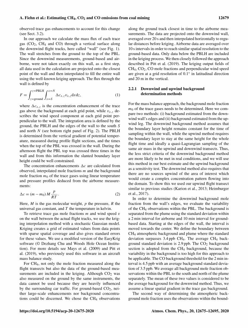
Figure 1. Flight track for flight B, color-coded with in-situ-measured CH4 mole fractions. The wind was blowing from the northeast over theUSCB (as indicated by the white wind barbs) carrying emissions to the southwest. Airborne observations averaged over 20 s are displayedas circles, and mobile ground observations averaged over 80 s below the upwind track and the downwind wall are marked as triangles. Redmarkers show the locations of active coal mine shafts from the CoMet v2 inventory.

craft and calibration technique. Details specific to the CoMetsetup can be found in the Supplement (Table S2 and Sect. S1in the Supplement). CO is measured with a modified quan-tum cascade laser spectrometer (QCLS) (Aerodyne) that alsorecords CO2, CH4, ethane (C2H6) and nitrous oxide (N2O)(Kostinek et al., 2019). Furthermore, a dry-air sampler with12 glass flasks (1 L) was installed aboard the Caravan, whichwere filled during the flight and later analyzed in the labo-ratory at the Max Planck Institute for Biogeochemistry fortrace gas concentrations and isotopic signatures (CH4, CO2,CO, N2O, H2, SF6, δ13C-CO2, δ18O-CO2, δ13C-CH4, δ2H-CH4). However, in this study we focus only on the continu-ous in situ observations, while the results of ethane measure-ments and isotopic signatures will be published in a follow-up study.

Ground-based CH4 data were recorded by three teamsusing vans equipped with different CRDS analyzers (Pi-carro G2201-i, AGH University and University of Heidel-berg; G2301, Utrecht University). The group from the AGHUniversity measured below the upwind leg and groups fromUniversity of Heidelberg and Utrecht University sampled be-low the downwind tracks. For traceability between airborne

and ground-based systems, an instrument intercomparisonwas conducted with the same four gas cylinders.

2.2 Mass balance method

We use a mass balance method to calculate emissionestimates for the USCB from two flights conducted on6 June. This approach is subject to several assumptions.First, the wind speed, wind direction, emissions and PBLHshould remain constant over the sampling time. Second,the trace gas plume has to be discernible from the atmo-spheric background. Third, there should not be any entrain-ment/detrainment into the free troposphere, and the lifetimeof the species must be much longer than transport and sam-pling times. Finally, the trace gas plume should be well-mixed between the lowest flight track and the ground. Thesecriteria are most likely to be met in the early afternoon,when the PBL has reached its maximum height and does notrise any further. The PBLH generally increases during themorning; hence afternoon flights are preferred over morningflights for mass balance studies. For our morning flight, wedetermine the temporal change of the PBLH during samplingto be 20 % of its final height. We apply a correction to the



observed trace gas enhancements to account for this change(see Sect. 3.2).

In our approach we calculate the mass flux of each tracegas (CO2, CH4 and CO) through a vertical surface alongthe downwind flight tracks, here called “wall” (see Fig. 1).The wall stretches from the ground to the top of the PBL.Since the downwind measurements, ground-based and air-borne, were not taken exactly on this wall, as a first step,all data used in the calculation are projected onto the closestpoint of the wall and then interpolated to fill the entire wallusing the well-known kriging approach. The flux through thewall is defined by

F =

∫ z=PBLH

z=ground

∫ x=N

x=S

1cx,zvx,zdxdz, (1)

where 1cx,z is the concentration enhancement of the tracegas above the background at each grid point, while vx,z de-scribes the wind speed component at each grid point per-pendicular to the wall. The integration area is defined by theground, the PBLH and the edges of the wall to the south Sand north N (see bottom right panel of Fig. 2). The PBLHis determined from the vertical gradient of potential temper-ature, measured during profile flight sections, and the timeswhen the top of the PBL was crossed in the wall. During theafternoon flight the PBL top was crossed three times in thewall and from this information the slanted boundary layerheight could be well constrained.

The concentration enhancements 1c are calculated fromobserved, interpolated mole fractions m and the backgroundmole fraction m0 of the trace gases using linear temperatureand pressure profiles deduced from the airborne measure-ments:

1c = (m−m0)Mp

RT. (2)

Here, M is the gas molecular weight, p the pressure, R theuniversal gas constant, and T the temperature in kelvin.

To retrieve trace gas mole fractions m and wind speed von the wall between the actual flight tracks, we use the krig-ing interpolation method with a stochastic Gaussian model.Kriging creates a grid of estimated values from data pointswith sparse spatial coverage and also gives standard errorsfor these values. We use a modified version of the EasyKrigsoftware (© Dezhang Chu and Woods Hole Ocean Institu-tion). For more details see Mays et al. (2009) and Pitt etal. (2019), who previously used this software in an aircraftmass balance study.

For CH4, not only the mole fraction measured along theflight transects but also the data of the ground-based mea-surements are included in the kriging. Although CO2 wasalso measured on the ground by the same instruments, thedata cannot be used because they are heavily influencedby the surrounding car traffic. For ground-based CO2, nei-ther large-scale enhancements nor background concentra-tions could be discerned. We chose the CH4 observations

along the ground track closest in time to the airborne mea-surements. The data are projected onto the downwind wall,averaged over 20 s and then interpolated horizontally to regu-lar distances before kriging. Airborne data are averaged over10 s intervals in order to reach similar spatial resolution to theground-based data. Only data below the PBLH are includedin the kriging process. We then closely followed the approachdescribed in Pitt et al. (2019). The kriging output fields ofCH4, CO2, CO mole fractions and perpendicular wind speedare given at a grid resolution of 0.1◦ in latitudinal directionand 20 m in the vertical.

2.2.1 Downwind and upwind backgrounddetermination methods

For the mass balance approach, the background mole fractionm0 of the trace gases needs to be determined. Here we com-pare two methods: (i) background estimated from the down-wind wall’s edges and (ii) background estimated from the up-wind leg. The downwind background method assumes thatthe boundary layer height remains constant for the time ofsampling within the wall, while the upwind method requiresthe boundary layer to stay at the same height for the wholeflight time and ideally a quasi-Lagrangian sampling of thesame air mass in the upwind and downwind transects. Thus,the less strict criteria of the downwind background methodare more likely to be met in real conditions, and we will usethis method in our best estimate and the upwind backgroundas a sensitivity test. The downwind method also requires thatthere are no sources upwind of the area of interest whichwould create a complex concentration pattern flowing intothe domain. To show this we used our upwind flight transectsimilar to previous studies (Karion et al., 2013; Heimburgeret al., 2017).

In order to determine the downwind background molefraction from the wall’s edges, we evaluate the variabilityof the CH4 observations within the PBL. The background isseparated from the plume using the standard deviation withina 2 min interval for airborne and 10 min interval for ground-based data. Starting at the edges of the wall, the interval ismoved towards the center. We define the boundary betweenCH4 atmospheric background and plume where the standarddeviation surpasses 3.4 ppb CH4. The average CH4 back-ground standard deviation is 2.9 ppb. The CO2 backgroundsection is adopted from the CH4 background, because thevariability in the background is too high for this approach tobe applicable. The CO background threshold for the 2 min in-terval is 4.5 ppb with an average background standard devia-tion of 3.5 ppb. We average all background mole fraction ob-servations within the PBL to the south and north of the plumeseparately. The mean of these two values is considered to bethe average background for the downwind method. Thus, weassume a linear spatial gradient in the trace gas background.

The second way of determining the atmospheric back-ground mole fraction uses the observations within the bound-



ary layer from the upwind flight transect, which was flownabout 15 min before the downwind wall and is here used in asensitivity study. Methodologically, we define a perpendicu-lar inflow transect according to the prevalent wind directionand project the upwind measurements onto this line (Supple-ment Fig. S1). After interpolation to regular distances, theaverage inflow mole fraction represents the upwind trace gasbackground. This approach has the advantage that sourcesupwind of the area of interest can be identified through po-tential enhancements in the upwind transect and are excludedfrom the emission estimate. On the other hand, the upwindbackground assumes that the same air masses are sampled inthe up- and downwind, which is not true for our two flights,since the air masses needed approximately 3–4 h to travelfrom the upwind to the downwind measurement location,while the aircraft only needed 15 min. The maximum timeseparation between up- and downwind sampling is 1.5 h.Thus, our sampling is not strictly Lagrangian (i.e. air massfollowing), and changes in boundary layer background con-centrations over time may affect the emission estimates usingthe upwind background method. Another disadvantage of us-ing upwind background concentrations with respect to CO2is the necessity to account for large-scale ground fluxes likethe biogenic uptake of CO2, which is discussed in the nextsection.

2.2.2 Simulation of biogenic uptake of CO2

We derive the influence of biogenic uptake of CO2 from acombination of backward trajectories, calculated using theStochastic Time-Inverted Lagrangian Transport (STILT; Linet al., 2003) model and biospheric fluxes from the VegetationPhotosynthesis and Respiration Model (VPRM; Mahadevanet al., 2008). STILT was set up with receptors distributedalong the flight track of the downwind wall and from eachreceptor, we then release 100 particles in the model. To drivethe trajectory simulations, we used output of the ECMWFHRES short-term forecasting system (approx. 9 km×9 kmspatial resolution, 137 vertical levels), preprocessed to assuremass conservation of the wind fields. The median locationsof the particle ensemble then constitute the median trajecto-ries (Fig. S2). The optimal use of the model in the method de-scribed would require the upwind track to be flown in exactlya Lagrangian manner, sampling the same air mass upwindand downwind of the sources. In our case, we have a singlehour of temporal difference in the observations and a 4 h dif-ference in the air-mass flow between measurement locations,during which the biosphere was able to uptake CO2. For thedifference in background mole fractions, the hour of biogenicuptake between upwind and downwind observations is rele-vant. The biospheric VPRM contribution to the downwindmeasurements is calculated using the footprint derived fromthe last hour of each trajectory, multiplied with the VPRMfluxes corresponding in time and location. We decided on thishybrid approach, in which we assume that we can still link

the measurements to our model quasi-directly, despite thefact that the model results are simulated for a location sev-eral tens of kilometers away from the actual upwind measure-ment location. It should be noted that it is assumed here thatthe biospheric fluxes are spatially homogeneous. We add thiscontribution to the downwind CO2 observation, only whenusing an upwind background, and then we use these valuesfor the interpolation with kriging.

2.3 Error estimate

For an error estimate of the derived mass flux, we considerthe statistical error of the input data and the systematic errorof the method.

2.3.1 Statistical error

The statistical error of our approach is determined using errorpropagation in the flux equation (Eqs. 1–2). The uncertaintycalculation of the concentration enhancement u1c, the fluxdensity uncertainty uFd and the final flux uncertainty uF aredescribed by Eqs. (3)–(5):

1c = c− c0→ u1c =

√u2c + u

2c0, (3)

Fd=1c · v→ uFd =

√(u1c1c

)2+

(uvv

)2·Fd, (4)

F =∑

iFdi ·A→ uF =

√∑i

(uFdi

)2·A. (5)

The first two uncertainties are calculated for each grid pointof the wall surface; the final flux uncertainty uF is the com-bination of the single uncertainties. The trace gas uncertaintyuc and wind speed uncertainty uv are a combination of mea-surement and kriging uncertainties expressed as kriging stan-dard error (KSE):

uc/v = umeasurement+KSE

= umeasurement+√ukriging · var(1c). (6)

The measurement uncertainty umeasurement has been deter-mined to 1.1 nmol mol−1 (hereafter referred to as parts perbillion) for CH4, 0.15 µmol mol−1 (hereafter referred to asparts per million) for CO2 (Table S2, Sect. S1) and 7 ppbfor CO (Kostinek et al., 2019). The wind speed measure-ment uncertainty uv has been assessed to be 0.3 m s−1 foreach of the horizontal components (Mallaun et al., 2015).The uncertainty of the interpolation and extrapolation krig-ing method is output by EasyKrig as a gridded field of nor-malized variance values ukriging. To retrieve the gridded KSE(see Fig. S4), which is equivalent to the standard deviation,we multiply the kriging error output ukriging by the varianceof the kriging input dataset 1c and then take the square root(Eq. 6). The background mole fraction uncertainty uc0 is heredefined as the standard deviation of all data points contribut-ing to the background calculation (see Table 4). The uncer-tainty of the grid cell area A is assumed to be zero.



2.3.2 Systematic error

We conducted several sensitivity tests in order to test the ro-bustness of our mass balance method and to determine itssystematic error. These sensitivity tests are described and dis-cussed in Sect. 3.4. We assume all systematic errors to be in-dependent and calculate the total absolute systematic error asthe square root of the sum of squared individual differencesfrom the best estimate, which treats the data as described inSect. 2.2 with a downwind trace gas background.

2.4 Bottom-up emission inventories

Several inventories of greenhouse gas and air pollutant emis-sions exist for the USCB. They vary in spatial and temporalresolution, as well as in the time for which they are available.Table 1 gives an overview of the six inventories we use in thisstudy for comparison with top-down-derived CH4, CO2 andCO emissions in the USCB region.

The first point source inventory listed in Table 1 is the Eu-ropean Emission Release and Transfer Register (E-PRTR).It results from the regulation (EC) no. 166/2006, which im-plements the United Nations Economic Commission for Eu-rope (UNECE) PRTR Protocol under which industrial fa-cilities have to report their emissions to air if they exceeda threshold of 100 t a−1 for CH4, 100 kt a−1 for CO2 and500 t a−1 for CO. Annual data can be downloaded from theEuropean Environmental Agency’s website (EEA, 2020).More information on the E-PRTR is given via its website:https://prtr.eea.europa.eu/ (last access: 24 February 2020).

The CoMet v2 inventory is a point source inventory basedon the E-PRTR 2016 emissions created by the CoMet teamespecially for this campaign. It comprises anthropogenicsources of CH4 and CO2 in the USCB and its vicinity. Thelargest difference between the E-PRTR and the CoMet inven-tory is that E-PRTR considers each coal mine to be one sin-gle point source, often located at the mining operator head-quarters, whereas in the CoMet inventory individual ventila-tion shafts were visually geo-localized using Google Earth.Then, the emission value of each mine was evenly distributedbetween all ventilation shafts belonging to that mine. Ac-tive Czech coal mines in the Ostrava region did not reportany CH4 emissions to E-PRTR but were assumed to emitthe same amount of CH4 per metric ton of extracted coalas Polish mines. We deduced a factor of 11.8± 5.2 kg CH4per metric ton of extracted coal for the USCB mines listed inTable S3 and applied this value to the Czech mines of Karv-iná, Karkov, CSM and Paskov. The locations of the 14 listedlandfills and waste disposal sites were checked against satel-lite imagery. Their CH4 emission is assumed to be 3.3 kt a−1,which is less than 1 % of the total USCB emissions.

Scarpelli et al. (2020) published the newest gridded emis-sion inventory available for comparison within this study. Itonly contains CH4 emissions from oil, natural gas and coalexploitation. But since these are the main sources (87 % ac-

cording to CAMS) of CH4 emissions in the USCB, valuesare comparable to the total of other inventories. Scarpelli etal. (2020) use the national totals of emissions reported tothe UNFCCC and distribute them according to the positionsof relevant infrastructure. Uncertainties of the emissions arebased on the emission factor uncertainties from the Intergov-ernmental Panel on Climate Change (IPCC) and are given asgridded information. Averaged over the USCB, the given rel-ative error standard deviation for CH4 emissions is 60.9 %.

The Copernicus Atmospheric Monitoring System(CAMS) regional emission inventory (CAMS-REG-GHG/AP; Granier et al., 2019) is based on the TNO-MACCinventories (Kuenen et al., 2014). This inventory offersa resolution twice as high as the Scarpelli and EDGARinventories. The inventory was also constructed by usingthe reported emission national totals by sector and spatiallydistributing them consistently across all countries by usingproxy parameters.

The most widely used gridded emission inventory is prob-ably the Emission Database for Global Atmospheric Re-search (EDGAR, https://data.europa.eu/doi/10.2904/JRC_DATASET_EDGAR, last access: 22 October 2020) globalemission inventory. The most recent version 5.0 (https://edgar.jrc.ec.europa.eu/overview.php?v=50_GHG, last ac-cess: 22 October 2020) includes emissions of the three ma-jor greenhouse gases CO2, CH4 and N2O. It is based on theprevious EDGAR version 4.3.2 (Janssens-Maenhout et al.,2019). We use the CO emissions from the air pollutant in-ventory (Crippa et al., 2018) from version 4.3.2. The mostrecent year of emission data is 2015 for CH4, 2018 for CO2and 2012 for CO. In EDGAR, annual country-specific emis-sions are derived from international activity data and emis-sion factors, which are then distributed in time and space us-ing monthly shares and spatial proxy datasets. The data in-clude uncertainty factors per species for three types of coun-tries: OECD countries of 1990, countries with economies intransition in 1990 and the remaining countries in develop-ment. European emissions from EDGAR in 2012 have stan-dard deviations of 16 % for CH4, 2.5 % for CO2 (Janssens-Maenhout et al., 2019) and 65 % for CO (Crippa et al.,2018).

The GESAPU inventory (Bun et al., 2019) has been cre-ated for Ukraine and Poland only for the reference year 2010.Originally, it is a point, line and area source inventory basedon shapefiles. The advantage of this type of information isthat it has a very high resolution but can also be gridded withany spatial resolution and orientation. The GESAPU inven-tory comprises all sectors of anthropogenic emissions. Herewe use a gridded version of the emissions with a resolutionof 15 arcsec (approximately 296m× 463 m for the region).

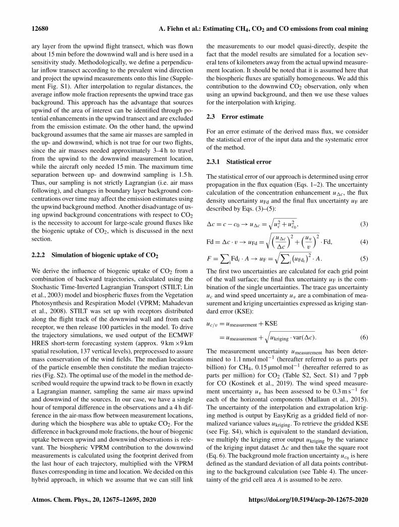
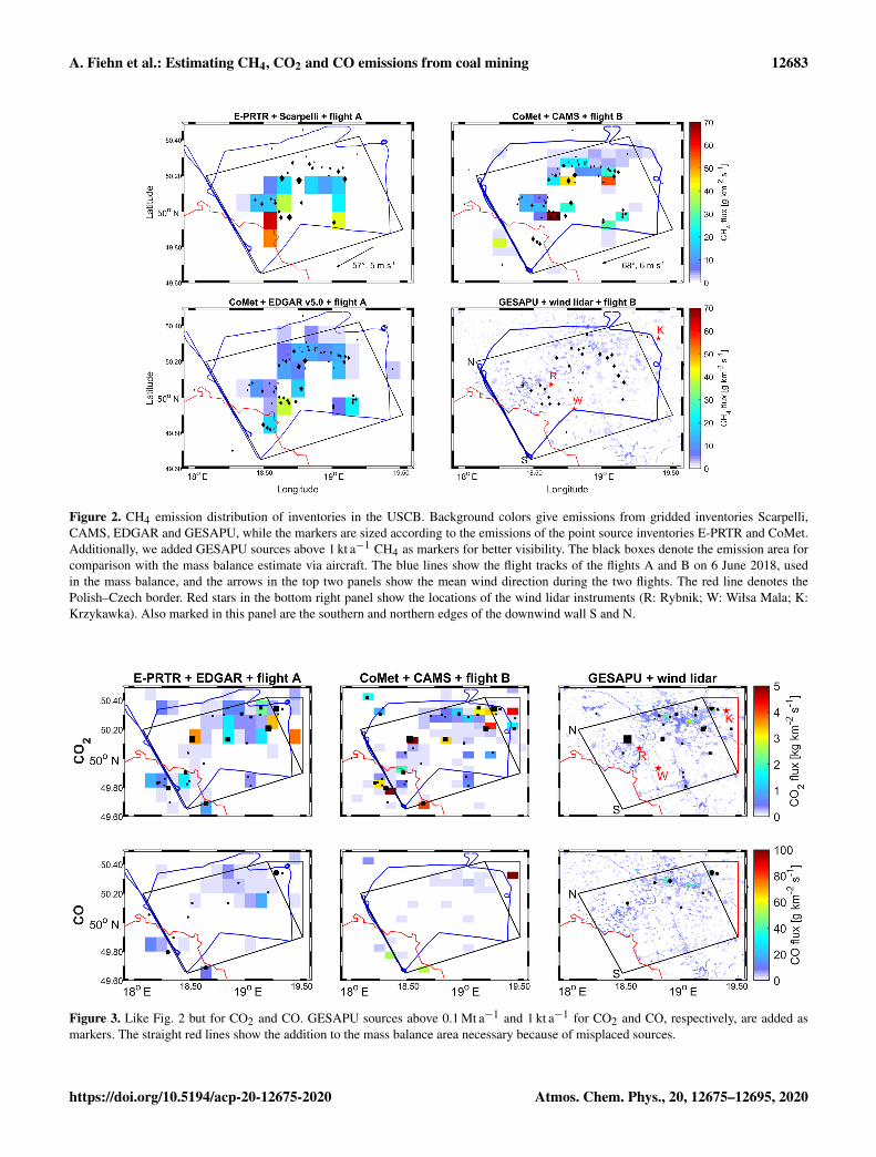
Figure 2 shows the spatial distribution of CH4 emissions asgiven by the six inventories. Point sources from E-PRTR andthe CoMet inventory are displayed as black markers whilethe background colors give the gridded inventory values. Al-though the inventories generally agree on the locations of


https://prtr.eea.europa.eu/

https://data.europa.eu/doi/10.2904/JRC_DATASET_EDGAR

https://data.europa.eu/doi/10.2904/JRC_DATASET_EDGAR

https://edgar.jrc.ec.europa.eu/overview.php?v=50_GHG

https://edgar.jrc.ec.europa.eu/overview.php?v=50_GHG


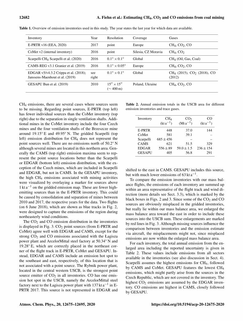
Table 1. Overview of emission inventories used in this study. The year states the last year for which data are available.

Inventory Year Resolution Coverage Gases

E-PRTR v16 (EEA, 2020) 2017 point Europe CH4, CO2, CO

CoMet v2 (internal inventory) 2016 point Silesia, CZ Moravia CH4, CO2

Scarpelli CH4 Scarpelli et al. (2020) 2016 0.1◦× 0.1◦ Global CH4 (Oil, Gas, Coal)

CAMS-REG v3.1 Granier et al. (2019) 2016 0.1◦× 0.05◦ Europe CH4, CO2, CO

EDGAR v5/v4.3.2 Crippa et al. (2018);Janssens-Maenhout et al. (2019)

seeright

0.1◦× 0.1◦ Global CH4 (2015), CO2 (2018), CO(2012)

GESAPU Bun et al. (2019) 2010 15′′× 15′′

(∼ 400 m)Poland, Ukraine CH4, CO2, CO

CH4 emissions, there are several cases where sources seemto be missing. Regarding point sources, E-PRTR (top left)has fewer individual sources than the CoMet inventory (topright) due to the separation in single ventilation shafts. Addi-tional mines in the CoMet inventory include the four Czechmines and the four ventilation shafts of the Brzeszcze minearound 19.15◦ E and 49.95◦ N. The gridded Scarpelli (topleft) emission distribution for CH4 does not represent thepoint sources well. There are no emissions north of 50.2◦ Nalthough several mines are located in this northern area. Gen-erally the CAMS (top right) emission maxima seem to rep-resent the point source locations better than the Scarpellior EDGAR (bottom left) emission distribution, with the ex-ception of the Czech mines, which are included in Scarpelliand EDGAR, but not in CAMS. In the GESAPU inventory,the high CH4 emissions associated with mining activitieswere visualized by overlaying a marker for sources above1 kt a−1 on the gridded emission map. These are fewer high-emitting sources than in the E-PRTR inventory. This couldbe caused by consolidation and separation of mines between2010 and 2017, the respective years for the data. Two flights(on 6 June 2018), which are shown as blue tracks in Fig. 2,were designed to capture the emissions of the region duringnortheasterly wind conditions.

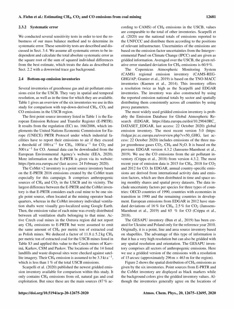
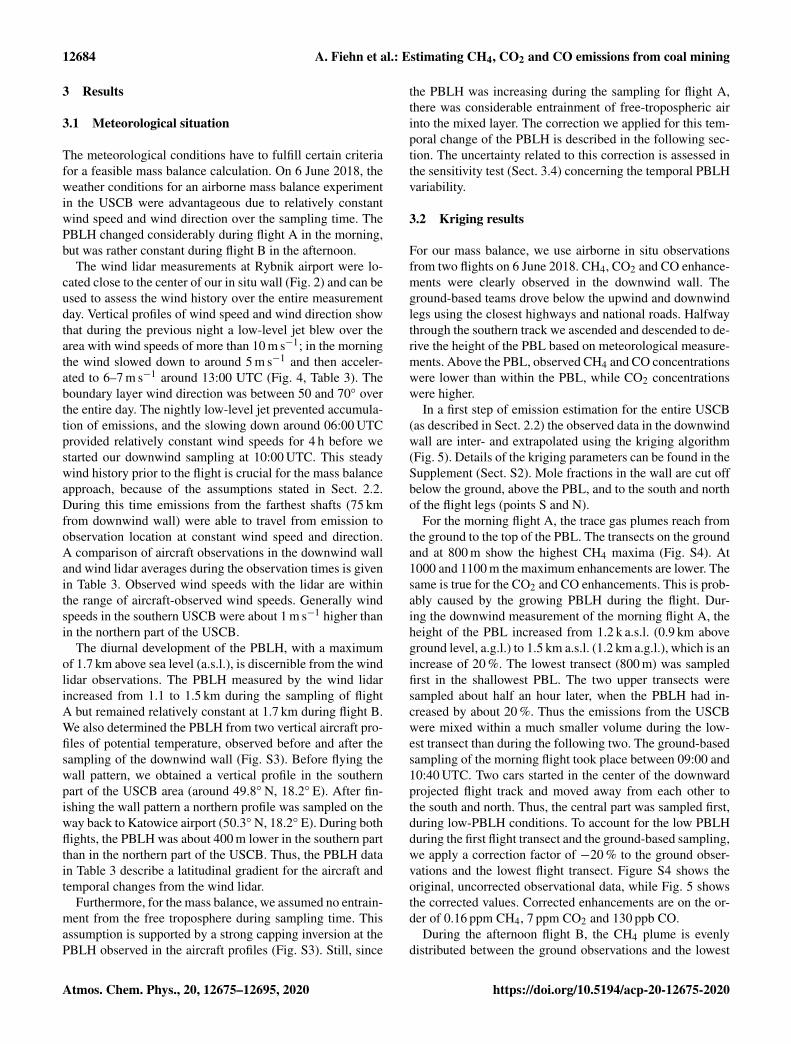
The CO2 and CO emission distribution in the inventoriesis displayed in Fig. 3. CO2 point sources (from E-PRTR andCoMet) agree well with EDGAR and CAMS, except for thestrong CO2 and CO emissions associated with the Łagiszapower plant and ArcelorMittal steel factory at 50.34◦ N and19.28◦ E, which are correctly placed in the northeast cor-ner of the flight track in E-PRTR, CoMet and GESAPU. In-stead, EDGAR and CAMS include an emission hot spot tothe southeast and east, respectively, of this location that isnot associated with a point source. The Rybnik power plant,located in the central western USCB, is the strongest pointsource emitter of CO2 in all inventories. CO has one emis-sion hot spot in the USCB, namely the ArcelorMittal steelfactory next to the Łagisza power plant with 137 kt a−1 in E-PRTR 2017. This source is not represented in EDGAR and

Table 2. Annual emission totals in the USCB area for differentemission inventories and trace gases.

Inventory CH4 CO2 CO(kt a−1) (Mt a−1) (kt a−1)

E-PRTR 448 37.0 144CoMet 581 39.1 –Scarpelli 685± 456 – –CAMS 621 51.5 329EDGAR 556± 89 59.0± 1.5 236± 154GESAPU 405 56.8 291

shifted to the east in CAMS. GESAPU includes this source,but with much lower emissions of 63 kt a−1.

To compare the emission inventories with our mass bal-ance flights, the emissions of each inventory are summed upwithin an area representative of the flight track and wind di-rection (more details see Sect. 3.3), which is marked by theblack boxes in Figs. 2 and 3. Since some of the CO2 and COsources are obviously misplaced in the gridded inventories,but really lie within our mass balance area, we enlarged themass balance area toward the east in order to include thesesources into the USCB sum. These enlargements are markedby red lines in Fig. 3. Although missing sources influence thecomparison between inventories and the emission estimatevia aircraft, the misplacements might not, since misplacedemissions are now within the enlarged mass balance area.

For each inventory, the total annual emission from the en-larged area including the reported uncertainty is given inTable 2. These values include emissions from all sectorsavailable in the inventories (see also discussion in Sect. 4).Scarpelli assumes the highest emissions for CH4, followedby CAMS and CoMet. GESAPU features the lowest CH4emissions, which might partly arise from the sources in theCzech Republic, which are not covered in the inventory. Thehighest CO2 emissions are assumed by the EDGAR inven-tory. CO emissions are highest in CAMS, closely followedby GESAPU.



Figure 2. CH4 emission distribution of inventories in the USCB. Background colors give emissions from gridded inventories Scarpelli,CAMS, EDGAR and GESAPU, while the markers are sized according to the emissions of the point source inventories E-PRTR and CoMet.Additionally, we added GESAPU sources above 1 kt a−1 CH4 as markers for better visibility. The black boxes denote the emission area forcomparison with the mass balance estimate via aircraft. The blue lines show the flight tracks of the flights A and B on 6 June 2018, usedin the mass balance, and the arrows in the top two panels show the mean wind direction during the two flights. The red line denotes thePolish–Czech border. Red stars in the bottom right panel show the locations of the wind lidar instruments (R: Rybnik; W: Wiłsa Mala; K:Krzykawka). Also marked in this panel are the southern and northern edges of the downwind wall S and N.

Figure 3. Like Fig. 2 but for CO2 and CO. GESAPU sources above 0.1 Mt a−1 and 1 kt a−1 for CO2 and CO, respectively, are added asmarkers. The straight red lines show the addition to the mass balance area necessary because of misplaced sources.



3 Results

3.1 Meteorological situation

The meteorological conditions have to fulfill certain criteriafor a feasible mass balance calculation. On 6 June 2018, theweather conditions for an airborne mass balance experimentin the USCB were advantageous due to relatively constantwind speed and wind direction over the sampling time. ThePBLH changed considerably during flight A in the morning,but was rather constant during flight B in the afternoon.

The wind lidar measurements at Rybnik airport were lo-cated close to the center of our in situ wall (Fig. 2) and can beused to assess the wind history over the entire measurementday. Vertical profiles of wind speed and wind direction showthat during the previous night a low-level jet blew over thearea with wind speeds of more than 10 m s−1; in the morningthe wind slowed down to around 5 m s−1 and then acceler-ated to 6–7 m s−1 around 13:00 UTC (Fig. 4, Table 3). Theboundary layer wind direction was between 50 and 70◦ overthe entire day. The nightly low-level jet prevented accumula-tion of emissions, and the slowing down around 06:00 UTCprovided relatively constant wind speeds for 4 h before westarted our downwind sampling at 10:00 UTC. This steadywind history prior to the flight is crucial for the mass balanceapproach, because of the assumptions stated in Sect. 2.2.During this time emissions from the farthest shafts (75 kmfrom downwind wall) were able to travel from emission toobservation location at constant wind speed and direction.A comparison of aircraft observations in the downwind walland wind lidar averages during the observation times is givenin Table 3. Observed wind speeds with the lidar are withinthe range of aircraft-observed wind speeds. Generally windspeeds in the southern USCB were about 1 m s−1 higher thanin the northern part of the USCB.

The diurnal development of the PBLH, with a maximumof 1.7 km above sea level (a.s.l.), is discernible from the windlidar observations. The PBLH measured by the wind lidarincreased from 1.1 to 1.5 km during the sampling of flightA but remained relatively constant at 1.7 km during flight B.We also determined the PBLH from two vertical aircraft pro-files of potential temperature, observed before and after thesampling of the downwind wall (Fig. S3). Before flying thewall pattern, we obtained a vertical profile in the southernpart of the USCB area (around 49.8◦ N, 18.2◦ E). After fin-ishing the wall pattern a northern profile was sampled on theway back to Katowice airport (50.3◦ N, 18.2◦ E). During bothflights, the PBLH was about 400 m lower in the southern partthan in the northern part of the USCB. Thus, the PBLH datain Table 3 describe a latitudinal gradient for the aircraft andtemporal changes from the wind lidar.

Furthermore, for the mass balance, we assumed no entrain-ment from the free troposphere during sampling time. Thisassumption is supported by a strong capping inversion at thePBLH observed in the aircraft profiles (Fig. S3). Still, since

the PBLH was increasing during the sampling for flight A,there was considerable entrainment of free-tropospheric airinto the mixed layer. The correction we applied for this tem-poral change of the PBLH is described in the following sec-tion. The uncertainty related to this correction is assessed inthe sensitivity test (Sect. 3.4) concerning the temporal PBLHvariability.

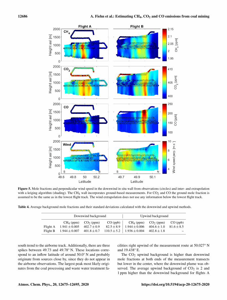
3.2 Kriging results

For our mass balance, we use airborne in situ observationsfrom two flights on 6 June 2018. CH4, CO2 and CO enhance-ments were clearly observed in the downwind wall. Theground-based teams drove below the upwind and downwindlegs using the closest highways and national roads. Halfwaythrough the southern track we ascended and descended to de-rive the height of the PBL based on meteorological measure-ments. Above the PBL, observed CH4 and CO concentrationswere lower than within the PBL, while CO2 concentrationswere higher.

In a first step of emission estimation for the entire USCB(as described in Sect. 2.2) the observed data in the downwindwall are inter- and extrapolated using the kriging algorithm(Fig. 5). Details of the kriging parameters can be found in theSupplement (Sect. S2). Mole fractions in the wall are cut offbelow the ground, above the PBL, and to the south and northof the flight legs (points S and N).

For the morning flight A, the trace gas plumes reach fromthe ground to the top of the PBL. The transects on the groundand at 800 m show the highest CH4 maxima (Fig. S4). At1000 and 1100 m the maximum enhancements are lower. Thesame is true for the CO2 and CO enhancements. This is prob-ably caused by the growing PBLH during the flight. Dur-ing the downwind measurement of the morning flight A, theheight of the PBL increased from 1.2 k a.s.l. (0.9 km aboveground level, a.g.l.) to 1.5 km a.s.l. (1.2 km a.g.l.), which is anincrease of 20 %. The lowest transect (800 m) was sampledfirst in the shallowest PBL. The two upper transects weresampled about half an hour later, when the PBLH had in-creased by about 20 %. Thus the emissions from the USCBwere mixed within a much smaller volume during the low-est transect than during the following two. The ground-basedsampling of the morning flight took place between 09:00 and10:40 UTC. Two cars started in the center of the downwardprojected flight track and moved away from each other tothe south and north. Thus, the central part was sampled first,during low-PBLH conditions. To account for the low PBLHduring the first flight transect and the ground-based sampling,we apply a correction factor of −20 % to the ground obser-vations and the lowest flight transect. Figure S4 shows theoriginal, uncorrected observational data, while Fig. 5 showsthe corrected values. Corrected enhancements are on the or-der of 0.16 ppm CH4, 7 ppm CO2 and 130 ppb CO.

During the afternoon flight B, the CH4 plume is evenlydistributed between the ground observations and the lowest



Figure 4. Wind speed and direction at Rybnik measured with a Doppler wind lidar on 6 June 2018. The bold line denotes the PBLHdetermined from the eddy dissipation rate and the thin vertical lines illustrate the downwind wall sampling times of flights A and B.

Table 3. Overview of wind data and PBLH from aircraft averaged within the downwind wall and wind lidar observations at Rybnik. Aircraftdata give uncertainty ranges due to measurement uncertainty, and wind lidar data state a standard deviation of the measurements within thePBL. The wind speed obtained from the lidar is additionally as an average over the 4 h previous to the downwind sampling.

Mean wind speed perpendicular (m s−1) Wind dir. (◦) PBLH (km a.s.l.)

Aircraft Wind lidar Aircraft Wind lidar Aircraft Wind lidar

Flight A (morning) 4.8± 0.3 to 5.7± 0.3 5.0± 0.9 and 5.1± 0.9 (4 h) 48± 2 57± 15 0.9± 0.05 and 1.25± 0.05 1.2± 0.05 to 1.5± 0.05Flight B (afternoon) 5.8± 0.3 to7.0± 0.3 6.4± 0.8 and 5.7± 1.0 (4 h) 62± 2 68± 12 1.3± 0.05 and 1.8± 0.05 1.7± 0.05

flight track at 800 m (Fig. 6). Thus, we assume good verticalmixing within the PBL and use the same CO2 and CO molefractions at the ground as in the lowest flight transect. Tracegas enhancements are on the order of 0.12 ppm CH4, 6 ppmCO2 and 120 ppb CO, thus lower than during the morningflight. The main CH4 plume is located at 50.0◦ N with a sec-ondary plume around 49.8◦ N. There are two CO2 plumes at50.0 and 50.1◦ N. The CO plume is located at 50.0◦ N.

The horizontal wind speed shows a latitudinal gradientwith higher wind speeds in the south than in the northfor both flights. This gradient is preserved when using akriged wind field for flux calculation instead of an averagewind speed for the whole downwind wall (as discussed inSect. 3.4).

Error estimates from the interpolation and extrapolationare retrieved from the kriging software as gridded fields (seeFig. S5). The KSE generally increases with distance to themeasurement locations and is highest at the ground for CO2,CO and wind speed because no ground-based measurementswere available for these parameters.

3.3 Background mole fractions

We applied both the downwind and the upwind methods (seeSect. 2.2.1) to determine atmospheric background mole frac-

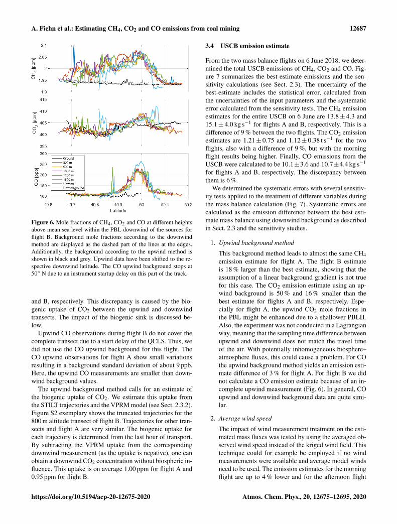
tions of trace gases. Average background mole fractions andstandard deviations for both methods are summarized in Ta-ble 4. Figure 6 shows the observed PBL mole fractions ofCH4, CO2 and CO at different heights for flight B. The high-est transect (light blue), originally planned in the free tropo-sphere above the PBL turned out to partially be within thePBL, but the southern and northern ends were sampled in thefree troposphere. The background mole fractions accordingto the downwind method are displayed as dotted lines. Forflight A, the background could not be reached to the southof the downwind wall, and only background values from thenorth were used for CH4 and CO2 (Fig. S4).

The upwind mole fractions (black lines) were shifted tothe corresponding latitudes of the downwind wall based onthe wind direction. The CH4 upwind mole fractions followthe same north–south gradient as the downwind background(Fig. 6, top). Around 49.94◦ N the CH4 mole fraction isslightly enhanced in the upwind. There is a similar enhance-ment around 50.13◦ N in flight A (Fig. S4). Due to the projec-tion, these would be between 50.2 and 50.3◦ N on the inflowtrack. The only source upwind of the inflow track in the in-ventories is the Trzebinia mine and power plant at 19.44◦ Eand 50.16◦ N. We use the ground-based observations belowthe upwind track (grey line) to confirm our aircraft observa-tions. They show similar absolute values and a similar north–



Figure 5. Mole fractions and perpendicular wind speed in the downwind in situ wall from observations (circles) and inter- and extrapolationwith a kriging algorithm (shading). The CH4 wall incorporates ground-based measurements. For CO2 and CO the ground mole fraction isassumed to be the same as in the lowest flight track. The wind extrapolation does not use any information below the lowest flight track.

Table 4. Average background mole fractions and their standard deviations calculated with the downwind and upwind methods.

Downwind background Upwind background

CH4 (ppm) CO2 (ppm) CO (ppb) CH4 (ppm) CO2 (ppm) CO (ppb)Flight A 1.941± 0.005 402.7± 0.9 82.5± 8.9 1.944± 0.006 404.6± 1.0 81.6± 8.5Flight B 1.944± 0.007 401.8± 0.7 110.5± 5.2 1.936± 0.004 402.8± 1.8 –

south trend to the airborne track. Additionally, there are threespikes between 49.73 and 49.78◦ N. These locations corre-spond to an inflow latitude of around 50.0◦ N and probablyoriginate from sources close by, since they do not appear inthe airborne observations. The largest peak most likely origi-nates from the coal processing and waste water treatment fa-

cilities right upwind of the measurement route at 50.027◦ Nand 19.438◦ E.

The CO2 upwind background is higher than downwindmole fractions at both ends of the measurement transectsbut lower in the center, where the downwind plume was ob-served. The average upwind background of CO2 is 2 and1 ppm higher than the downwind background for flights A



Figure 6. Mole fractions of CH4, CO2 and CO at different heightsabove mean sea level within the PBL downwind of the sources forflight B. Background mole fractions according to the downwindmethod are displayed as the dashed part of the lines at the edges.Additionally, the background according to the upwind method isshown in black and grey. Upwind data have been shifted to the re-spective downwind latitude. The CO upwind background stops at50◦ N due to an instrument startup delay on this part of the track.

and B, respectively. This discrepancy is caused by the bio-genic uptake of CO2 between the upwind and downwindtransects. The impact of the biogenic sink is discussed be-low.

Upwind CO observations during flight B do not cover thecomplete transect due to a start delay of the QCLS. Thus, wedid not use the CO upwind background for this flight. TheCO upwind observations for flight A show small variationsresulting in a background standard deviation of about 9 ppb.Here, the upwind CO measurements are smaller than down-wind background values.

The upwind background method calls for an estimate ofthe biogenic uptake of CO2. We estimate this uptake fromthe STILT trajectories and the VPRM model (see Sect. 2.3.2).Figure S2 exemplary shows the truncated trajectories for the800 m altitude transect of flight B. Trajectories for other tran-sects and flight A are very similar. The biogenic uptake foreach trajectory is determined from the last hour of transport.By subtracting the VPRM uptake from the correspondingdownwind measurement (as the uptake is negative), one canobtain a downwind CO2 concentration without biospheric in-fluence. This uptake is on average 1.00 ppm for flight A and0.95 ppm for flight B.

3.4 USCB emission estimate

From the two mass balance flights on 6 June 2018, we deter-mined the total USCB emissions of CH4, CO2 and CO. Fig-ure 7 summarizes the best-estimate emissions and the sen-sitivity calculations (see Sect. 2.3). The uncertainty of thebest-estimate includes the statistical error, calculated fromthe uncertainties of the input parameters and the systematicerror calculated from the sensitivity tests. The CH4 emissionestimates for the entire USCB on 6 June are 13.8± 4.3 and15.1± 4.0 kg s−1 for flights A and B, respectively. This is adifference of 9 % between the two flights. The CO2 emissionestimates are 1.21± 0.75 and 1.12± 0.38 t s−1 for the twoflights, also with a difference of 9 %, but with the morningflight results being higher. Finally, CO emissions from theUSCB were calculated to be 10.1±3.6 and 10.7±4.4 kg s−1

for flights A and B, respectively. The discrepancy betweenthem is 6 %.

We determined the systematic errors with several sensitiv-ity tests applied to the treatment of different variables duringthe mass balance calculation (Fig. 7). Systematic errors arecalculated as the emission difference between the best esti-mate mass balance using downwind background as describedin Sect. 2.3 and the sensitivity studies.

1. Upwind background method

This background method leads to almost the same CH4emission estimate for flight A. The flight B estimateis 18 % larger than the best estimate, showing that theassumption of a linear background gradient is not truefor this case. The CO2 emission estimate using an up-wind background is 50 % and 16 % smaller than thebest estimate for flights A and B, respectively. Espe-cially for flight A, the upwind CO2 mole fractions inthe PBL might be enhanced due to a shallower PBLH.Also, the experiment was not conducted in a Lagrangianway, meaning that the sampling time difference betweenupwind and downwind does not match the travel timeof the air. With potentially inhomogeneous biosphere–atmosphere fluxes, this could cause a problem. For COthe upwind background method yields an emission esti-mate difference of 3 % for flight A. For flight B we didnot calculate a CO emission estimate because of an in-complete upwind measurement (Fig. 6). In general, COupwind and downwind background data are quite simi-lar.

2. Average wind speed

The impact of wind measurement treatment on the esti-mated mass fluxes was tested by using the averaged ob-served wind speed instead of the kriged wind field. Thistechnique could for example be employed if no windmeasurements were available and average model windsneed to be used. The emission estimates for the morningflight are up to 4 % lower and for the afternoon flight



Figure 7. USCB emission estimates on 6 June 2018, using an airborne mass balance approach including several sensitivity tests.

up to 13 % higher than for the best estimate. Here thesystematic change in the emission estimates is causedby the location of the plume in the wind field. Duringflight A, the plumes were located where the wind speedwas slightly higher than average (see Fig. 5). Using theaverage wind speed, thus, results in a reduction of theemission estimates. During flight B, the plume locationswere in a slow wind region with higher wind speeds tothe south, especially for the CO2 and CO plumes. Us-ing averaged wind speed, thus, enhanced the emissionestimate. We highlight the importance of measuring thewind speed simultaneously with the mole fractions andusing this spatial knowledge in the flux calculation.

3. Wind speed variability

One assumption for a mass balance calculation is thatthe wind speed and direction are constant during thetime it takes for the gases to be transported from theemission source to the observation location. In realitythe wind field can be subject to considerable variability.In our case we were able to assess this temporal vari-ability from the wind lidar observations. To account forwind variability we calculated the standard deviation ofwind speed during the 4 h transit time within the bound-ary layer and added it to the kriged wind field used inthe mass balance calculation. This introduced an uncer-tainty of 17 % and 15 % to the morning and afternoonflight results, respectively.

4. Ground data uncertainty

Since we did not use CO2 and CO from the mobileground measurements, we calculated the sensitivity ofour approach to the precise knowledge of ground-baseddata for CO2 and CO. Assuming a 10 % uncertainty ofthe ground value enhancements and increasing the krig-ing input ground values by this factor result in a system-atic error of 15 %–20 %. This shows that a good approx-imation, or even better a measurement, of mole fractionsbelow the lowest flight track is important for exact emis-sion estimates.

5. PBLH uncertainty

Another sensitivity of our method is related to theknowledge of the PBLH and its variability. Its exact de-termination in the downwind wall is only possible whenwe cross its top during ascents or descents. This oc-curred once during the morning flight and three times inthe afternoon. The PBLH is further constrained by ver-tical profiles before and after sampling the downwindwall and through the wind lidar observations. These datahint at temporal and spatial variations in the PBLH (seeSect. 3.1). Based on these data we assign an uncertaintyestimate of 100 m to PBLH. We account for the spa-tial PBLH uncertainty in the emission estimate by usinga boundary layer 100 m higher than our best estimate.This is realized through cutting off the flux density fieldat this increased boundary. For this sensitivity test, dis-crepancies are between 5 % and 12 % for all three gases.

6. Temporal PBLH variability

The last sensitivity test accounts for the temporal vari-ation in the PBLH during the morning flight A. ThePBLH showed a temporal variability of 300 m, quan-tifiable from wind lidar measurements. We assess theuncertainty caused by the temporally increasing PBLHfor the morning flight by omitting the trace gas enhance-ment correction described in Sect. 3.2. The systematicerror for flight A is between 21 % and 23 %.

On average, the uncertainty of the background molefraction (up to 50 %), the uncertainty of mole frac-tions at the ground (15 %–20 %) and the wind variability(15 %–17 %) have the highest impact on the systematicuncertainty. For flight A, the changing PBLH introducesan additional 21 %–23 % uncertainty to the emission es-timates. Assuming that the single systematic uncertain-ties are independent of each other, the total systematicerror of the emission estimate is calculated as the squareroot of the sum of squared individual uncertainties andis added to the statistical uncertainty. The statistical er-ror is 1 % for CH4 and around 3 % for CO2 and CO and,



thus, small compared to the systematic errors of this ap-proach. It is added to the systematic error to obtain thetotal error of the emission estimates. The CH4 emissionestimate has a total relative error of 31 % and 26 %, aCO2 estimate of 62 % and 37 %, and a CO estimate of36 % and 41 % for flights A and B, respectively. The er-rors are mostly larger for flight A than for flight B, sincethe afternoon flight is more suitable for a mass balanceexperiment due to the temporally constant PBLH.

3.5 Single-transect emission estimates

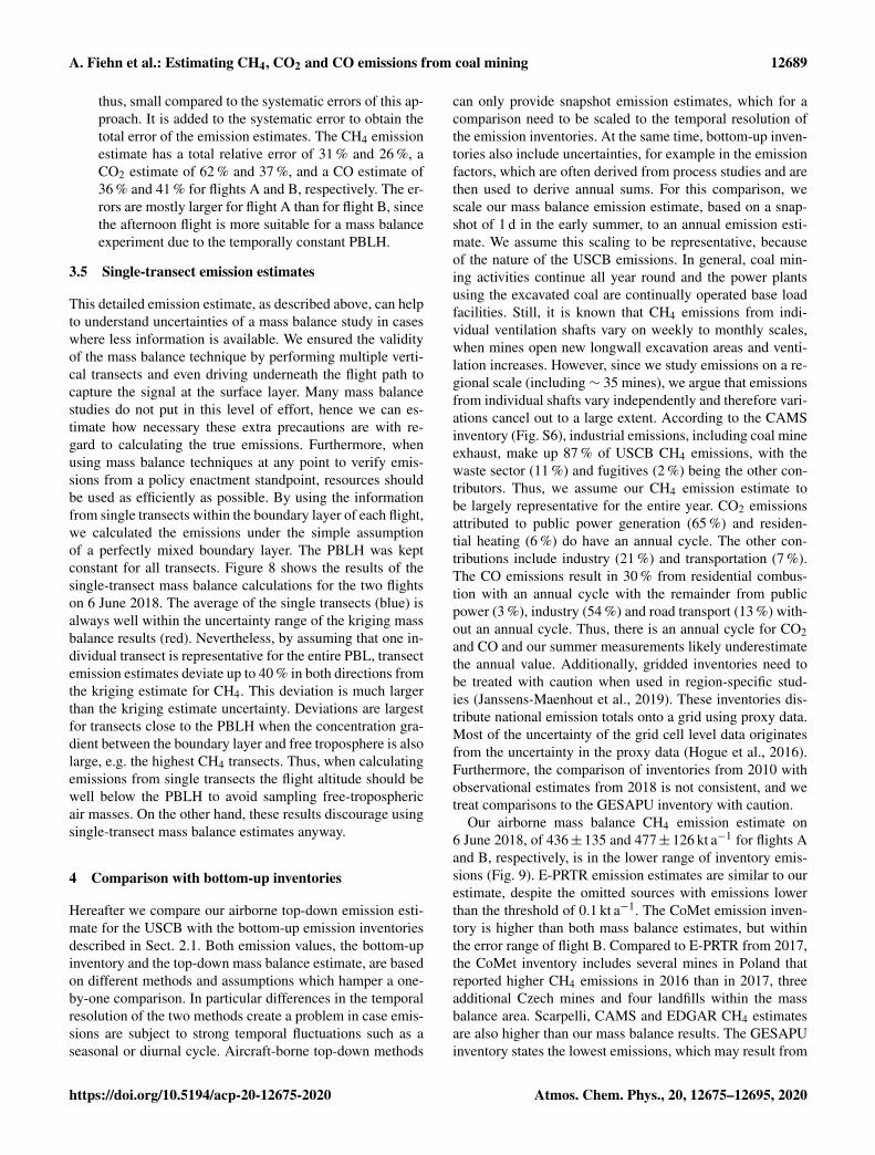
This detailed emission estimate, as described above, can helpto understand uncertainties of a mass balance study in caseswhere less information is available. We ensured the validityof the mass balance technique by performing multiple verti-cal transects and even driving underneath the flight path tocapture the signal at the surface layer. Many mass balancestudies do not put in this level of effort, hence we can es-timate how necessary these extra precautions are with re-gard to calculating the true emissions. Furthermore, whenusing mass balance techniques at any point to verify emis-sions from a policy enactment standpoint, resources shouldbe used as efficiently as possible. By using the informationfrom single transects within the boundary layer of each flight,we calculated the emissions under the simple assumptionof a perfectly mixed boundary layer. The PBLH was keptconstant for all transects. Figure 8 shows the results of thesingle-transect mass balance calculations for the two flightson 6 June 2018. The average of the single transects (blue) isalways well within the uncertainty range of the kriging massbalance results (red). Nevertheless, by assuming that one in-dividual transect is representative for the entire PBL, transectemission estimates deviate up to 40 % in both directions fromthe kriging estimate for CH4. This deviation is much largerthan the kriging estimate uncertainty. Deviations are largestfor transects close to the PBLH when the concentration gra-dient between the boundary layer and free troposphere is alsolarge, e.g. the highest CH4 transects. Thus, when calculatingemissions from single transects the flight altitude should bewell below the PBLH to avoid sampling free-troposphericair masses. On the other hand, these results discourage usingsingle-transect mass balance estimates anyway.

4 Comparison with bottom-up inventories

Hereafter we compare our airborne top-down emission esti-mate for the USCB with the bottom-up emission inventoriesdescribed in Sect. 2.1. Both emission values, the bottom-upinventory and the top-down mass balance estimate, are basedon different methods and assumptions which hamper a one-by-one comparison. In particular differences in the temporalresolution of the two methods create a problem in case emis-sions are subject to strong temporal fluctuations such as aseasonal or diurnal cycle. Aircraft-borne top-down methods

can only provide snapshot emission estimates, which for acomparison need to be scaled to the temporal resolution ofthe emission inventories. At the same time, bottom-up inven-tories also include uncertainties, for example in the emissionfactors, which are often derived from process studies and arethen used to derive annual sums. For this comparison, wescale our mass balance emission estimate, based on a snap-shot of 1 d in the early summer, to an annual emission esti-mate. We assume this scaling to be representative, becauseof the nature of the USCB emissions. In general, coal min-ing activities continue all year round and the power plantsusing the excavated coal are continually operated base loadfacilities. Still, it is known that CH4 emissions from indi-vidual ventilation shafts vary on weekly to monthly scales,when mines open new longwall excavation areas and venti-lation increases. However, since we study emissions on a re-gional scale (including∼ 35 mines), we argue that emissionsfrom individual shafts vary independently and therefore vari-ations cancel out to a large extent. According to the CAMSinventory (Fig. S6), industrial emissions, including coal mineexhaust, make up 87 % of USCB CH4 emissions, with thewaste sector (11 %) and fugitives (2 %) being the other con-tributors. Thus, we assume our CH4 emission estimate tobe largely representative for the entire year. CO2 emissionsattributed to public power generation (65 %) and residen-tial heating (6 %) do have an annual cycle. The other con-tributions include industry (21 %) and transportation (7 %).The CO emissions result in 30 % from residential combus-tion with an annual cycle with the remainder from publicpower (3 %), industry (54 %) and road transport (13 %) with-out an annual cycle. Thus, there is an annual cycle for CO2and CO and our summer measurements likely underestimatethe annual value. Additionally, gridded inventories need tobe treated with caution when used in region-specific stud-ies (Janssens-Maenhout et al., 2019). These inventories dis-tribute national emission totals onto a grid using proxy data.Most of the uncertainty of the grid cell level data originatesfrom the uncertainty in the proxy data (Hogue et al., 2016).Furthermore, the comparison of inventories from 2010 withobservational estimates from 2018 is not consistent, and wetreat comparisons to the GESAPU inventory with caution.

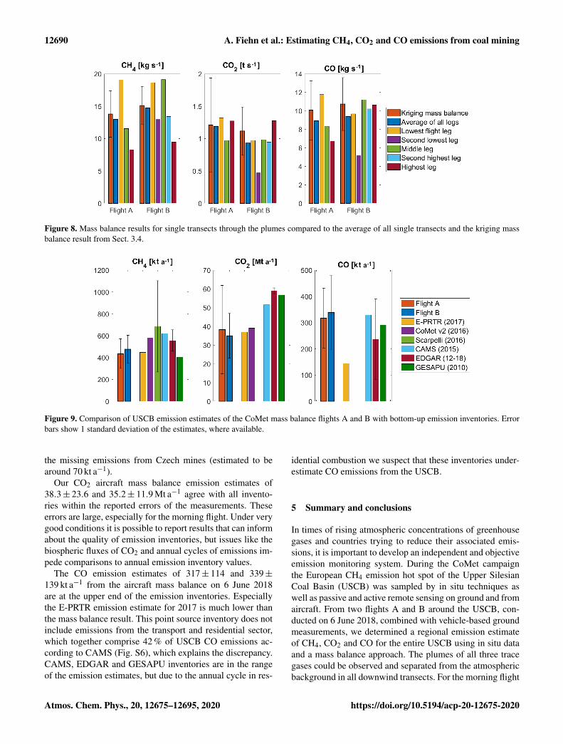
Our airborne mass balance CH4 emission estimate on6 June 2018, of 436± 135 and 477± 126 kt a−1 for flights Aand B, respectively, is in the lower range of inventory emis-sions (Fig. 9). E-PRTR emission estimates are similar to ourestimate, despite the omitted sources with emissions lowerthan the threshold of 0.1 kt a−1. The CoMet emission inven-tory is higher than both mass balance estimates, but withinthe error range of flight B. Compared to E-PRTR from 2017,the CoMet inventory includes several mines in Poland thatreported higher CH4 emissions in 2016 than in 2017, threeadditional Czech mines and four landfills within the massbalance area. Scarpelli, CAMS and EDGAR CH4 estimatesare also higher than our mass balance results. The GESAPUinventory states the lowest emissions, which may result from



Figure 8. Mass balance results for single transects through the plumes compared to the average of all single transects and the kriging massbalance result from Sect. 3.4.

Figure 9. Comparison of USCB emission estimates of the CoMet mass balance flights A and B with bottom-up emission inventories. Errorbars show 1 standard deviation of the estimates, where available.

the missing emissions from Czech mines (estimated to bearound 70 kt a−1).

Our CO2 aircraft mass balance emission estimates of38.3± 23.6 and 35.2± 11.9 Mt a−1 agree with all invento-ries within the reported errors of the measurements. Theseerrors are large, especially for the morning flight. Under verygood conditions it is possible to report results that can informabout the quality of emission inventories, but issues like thebiospheric fluxes of CO2 and annual cycles of emissions im-pede comparisons to annual emission inventory values.

The CO emission estimates of 317± 114 and 339±139 kt a−1 from the aircraft mass balance on 6 June 2018are at the upper end of the emission inventories. Especiallythe E-PRTR emission estimate for 2017 is much lower thanthe mass balance result. This point source inventory does notinclude emissions from the transport and residential sector,which together comprise 42 % of USCB CO emissions ac-cording to CAMS (Fig. S6), which explains the discrepancy.CAMS, EDGAR and GESAPU inventories are in the rangeof the emission estimates, but due to the annual cycle in res-

idential combustion we suspect that these inventories under-estimate CO emissions from the USCB.

5 Summary and conclusions

In times of rising atmospheric concentrations of greenhousegases and countries trying to reduce their associated emis-sions, it is important to develop an independent and objectiveemission monitoring system. During the CoMet campaignthe European CH4 emission hot spot of the Upper SilesianCoal Basin (USCB) was sampled by in situ techniques aswell as passive and active remote sensing on ground and fromaircraft. From two flights A and B around the USCB, con-ducted on 6 June 2018, combined with vehicle-based groundmeasurements, we determined a regional emission estimateof CH4, CO2 and CO for the entire USCB using in situ dataand a mass balance approach. The plumes of all three tracegases could be observed and separated from the atmosphericbackground in all downwind transects. For the morning flight



A, a trace gas enhancement correction was employed to ac-count for the temporal change of PBLH during the sam-pling. We employed a kriging algorithm for the interpola-tion of observed CH4, CO2, CO and wind speed between theflight transects and towards the ground. CH4 ground-basedobservations confirmed the existence of a well-mixed PBLwith similar trace gas enhancements at the ground and in theaircraft transects. From the kriged fields we calculated theUSCB emission estimate as the mass flux through the down-wind wall for each flight. Using error propagation and sev-eral sensitivity tests, we carefully determined the total errorof our mass balance approach. The CH4 emission estimatehas a total relative error of 26 %–31 %, the CO2 estimate of37 %–62 % and the CO estimate of 36 %–41 %. These un-certainties are mainly caused by the background determina-tion, wind speed variability and missing knowledge of molefractions below the lowest flight track for CO2 and CO. Thehigher uncertainty values apply to the morning flight esti-mate, because the temporal variation in the PBLH introduceda large error. Thus, we highlight the importance of a constantPBLH over time, knowledge of trace gas mole fractions at theground and the exact knowledge of background mole frac-tions. The large uncertainties in the CO2 estimate are dom-inated by the uncertainties in biospheric CO2 fluxes. Theseestimates could be improved by performing flights in winter-time, when the biospheric fluxes are negligible. Flights dur-ing different seasons would also better constrain the annualcycle in CO2 emissions from the residential sector. The cal-culation of emission estimates from single flight transects isnot advisable, because the single-transect estimates showeddeviations from their mean and the kriging method of morethan 40 % in both directions.

The CoMet in situ CH4 emissions estimates from6 June 2018, of 13.8± 4.3 and 15.1± 4.0 kg s−1 for flightsA and B, respectively, are in the lower range of the six pre-sented emission inventories. This agreement of our indepen-dent USCB emission estimate with the bottom-up coal min-ing emission reports indicates that this sector of emissionsis well understood and monitored on regional scales. Theemissions of CO2 were determined to be 1.21± 0.75 and1.12± 0.38 t s−1. The estimate from the second flight con-strains the emissions to the lower end of inventory values.The gridded inventories, which report higher emissions thanour estimate, do not include an annual cycle in the residentialcombustion emissions of CO2. This might be reflected in ourlow summer emission estimate. In general, an airborne massbalance estimate for CO2 on these spatial scales is difficultdue to inhomogeneous biospheric uptake. CO mass balanceemissions of 10.1±3.6 and 10.7±4.4 kg s−1 for the USCB on6 June 2018 are much higher than the E-PRTR point sourceinventory, which does not include residential combustion androad transport emissions and are still in the upper range ofthe gridded emission inventory values. The comparison be-tween the snapshot top-down emission estimate and annualbottom-up inventories is influenced by the temporal variabil-

ity of emissions in the USCB. Therefore, additional measure-ments during different seasons are needed to finally confirmbottom-up emission inventories.

Our airborne in situ mass balance method describes a mea-surement and evaluation strategy, which can be applied forvarious emission sources on a local to regional scale. In thiscase, we provide an independent bottom-up emission assess-ment for the USCB, which also serves as a point of refer-ence for other state-of-the-art techniques, like airborne lidarand passive spectroscopy. A comparison of in situ and remotesensing emission estimation techniques will follow in futurestudies.

Independent top-down validation of emissions in industri-alized countries can confirm the statistical approaches usedin bottom-up inventories. Once facility locations and activ-ity, technology, and abatement information becomes avail-able for other countries or regions, the confirmed emissionsfrom industrialized areas will help to improve global emis-sion inventories used in climate projections. These will inturn help policy makers to develop efficient climate mitiga-tion strategies. Consistent, reliable and timely informationon greenhouse gas emissions will allow the implementation,evaluation and management of long-term policies that mightallow keeping the global temperature rise below 2 ◦C abovepreindustrial levels.

Data availability. The data are accessible on the ICOS ERIC – Car-bon Portal under https://doi.org/10.18160/0SFH-JJ93 (Fiehn et al.,2020).

Supplement. The supplement related to this article is available on-line at: https://doi.org/10.5194/acp-20-12675-2020-supplement.

Author contributions. AF, JK and ME performed the trace gas mea-surements, calibrations and data preparation. AF analyzed the dataand drafted the manuscript. TK provided shaft-wise E-PRTR ge-olocation and emission data retrieved from the E-PRTR dataset andthe Polish State Mining Authority for 2014. This dataset was up-dated and expanded by MG to the used version 2. MG, JC and CGprovided STILT and VPRM simulations and helpful discussions onbiogenic uptake of CO2. TR coordinated the deployment of ground-based measurements and helped with data evaluation and interpre-tation. HM, MS, PK and JN conducted ground-based in situ mea-surements in the field during the campaign and collected and sharedthe data. PJ conducted ground-based observations and supported theaircraft observations through coordinating the airport communica-tions at Rybnik airport. NW took an active part during the campaigndeploying the wind lidar and retrieving and providing wind lidardata. CM supervised the wind measurements on board the CessnaCaravan and prepared the data. RB provided a gridded version ofthe GESAPU emission inventory for the USCB. ALN and PJ de-vised, set up and supervised the forecasting system that allowedflight planning for the CoMet campaign in the USCB. AF coordi-


https://doi.org/10.18160/0SFH-JJ93

https://doi.org/10.5194/acp-20-12675-2020-supplement


nated all CoMet campaign contributions. AR developed the researchidea and coordinated the CoMet Cessna campaign operations.

All authors contributed to the interpretation of the results and theimprovement of the manuscript.

Competing interests. The authors declare that they have no conflictof interest.

Special issue statement. This article is part of the special issue“CoMet: a mission to improve our understanding and to better quan-tify the carbon dioxide and methane cycles”. It is not associatedwith a conference.

Acknowledgements. The authors especially thank DLR-FX for thecampaign cooperation, especially the pilots Thomas van Mar-wick and Philipp Weber and the group of Ralph Helmes, An-dreas Giez, Martin Zöger and Martin Sedlmeir. We would like tothank Joseph Pitt for providing an updated version of the krigingpackage and giving advice on its usage. We acknowledge fundingfor the CoMet campaign by BMBF (German Federal Ministry ofEducation and Research) through AIRSPACE. We thank DLR VO-R for funding the young investigator research group “GreenhouseGases”. The ground-based measurements on vehicles were fundedby the European Union’s Horizon 2020 Research and Innovationprogram under the Marie Skłodowska-Curie ITN project Methanegoes Mobile – Measurements and Modelling (MEMO2; https://h2020-memo2.eu/, last access: 22 October 2020). The authors ac-knowledge ECCAD for archiving and distributing the CAMS emis-sion inventories.

Financial support. This research has been supported by the BMBF(grant nos. FKZ 01LK1701A and FKZ 01LK1701C), the EUHorizon 2020 MEMO2 (grant no. 722479), and the DeutscheForschungsgemeinschaft (DFG) Priority Program SPP 1294.

The article processing charges for this open-access publica-tion were covered by a Research Centre of the HelmholtzAssociation.

Review statement. This paper was edited by Anita Ganesan and re-viewed by Anna Karion and Zachary Barkley.

References

Alvarez, R. A., Zavala-Araiza, D., Lyon, D. R., Allen, D. T.,Barkley, Z. R., Brandt, A. R., Davis, K. J., Herndon, S.C., Jacob, D. J., Karion, A., Kort, E. A., Lamb, B. K.,Lauvaux, T., Maasakkers, J. D., Marchese, A. J., Omara,M., Pacala, S. W., Peischl, J., Robinson, A. L., Shepson,P. B., Sweeney, C., Townsend-Small, A., Wofsy, S. C., andHamburg, S. P.: Assessment of methane emissions from

the U.S. oil and gas supply chain, Science, 361, 186–188,https://doi.org/10.1126/science.aar7204, 2018.

Amediek, A., Ehret, G., Fix, A., Wirth, M., Büdenbender, C., Qua-trevalet, M., Kiemle, C., and Gerbig, C.: CHARM-F – a newairborne integrated-path differential-absorption lidar for carbondioxide and methane observations: measurement performanceand quantification of strong point source emissions, Appl. Opt.,56, 5182–5197, https://doi.org/10.1364/AO.56.005182, 2017.

Barkley, Z. R., Lauvaux, T., Davis, K. J., Deng, A., Fried, A.,Weibring, P., Richter, D., Walega, J. G., DiGangi, J., Ehrman,S. H., Ren, X., and Dickerson, R. R.: Estimating MethaneEmissions From Underground Coal and Natural Gas Productionin Southwestern Pennsylvania, Geophys. Res. Lett., 46, 4531–4540, https://doi.org/10.1029/2019gl082131, 2019.

Bergamaschi, P., Karstens, U., Manning, A. J., Saunois, M., Tsu-ruta, A., Berchet, A., Vermeulen, A. T., Arnold, T., Janssens-Maenhout, G., Hammer, S., Levin, I., Schmidt, M., Ramonet,M., Lopez, M., Lavric, J., Aalto, T., Chen, H., Feist, D. G., Ger-big, C., Haszpra, L., Hermansen, O., Manca, G., Moncrieff, J.,Meinhardt, F., Necki, J., Galkowski, M., O’Doherty, S., Para-monova, N., Scheeren, H. A., Steinbacher, M., and Dlugo-kencky, E.: Inverse modelling of European CH4 emissions dur-ing 2006–2012 using different inverse models and reassessedatmospheric observations, Atmos. Chem. Phys., 18, 901–920,https://doi.org/10.5194/acp-18-901-2018, 2018.

Brioude, J., Angevine, W. M., Ahmadov, R., Kim, S.-W., Evan, S.,McKeen, S. A., Hsie, E.-Y., Frost, G. J., Neuman, J. A., Pol-lack, I. B., Peischl, J., Ryerson, T. B., Holloway, J., Brown,S. S., Nowak, J. B., Roberts, J. M., Wofsy, S. C., Santoni, G.W., Oda, T., and Trainer, M.: Top-down estimate of surface fluxin the Los Angeles Basin using a mesoscale inverse modelingtechnique: assessing anthropogenic emissions of CO, NOx andCO2 and their impacts, Atmos. Chem. Phys., 13, 3661–3677,https://doi.org/10.5194/acp-13-3661-2013, 2013.

Bun, R., Nahorski, Z., Horabik-Pyzel, J., Danylo, O., See, L.,Charkovska, N., Topylko, P., Halushchak, M., Lesiv, M., Valakh,M., and Kinakh, V.: Development of a high-resolution spatial in-ventory of greenhouse gas emissions for Poland from station-ary and mobile sources, Mitig. Adapt. Strat. Gl., 24, 853–880,https://doi.org/10.1007/s11027-018-9791-2, 2019.

Cambaliza, M. O. L., Shepson, P. B., Bogner, J., Caulton,D.R., Stirm, B., Sweeney, C., Montzka, S.A., Gurney, K.R.,Spokas, K., Salmon, O.E., Lavoie, T.N., Hendricks, A., Mays,K., Turnbull, J., Miller, B.R., Lauvaux, T., Davis, K., Kar-ion, A., Moser, B., Miller, C., Obermeyer, C., Whetstone,J., Prasad, K., Miles, N., and Richardson, S.: Quantifica-tion and source apportionment of the methane emission fluxfrom the city of Indianapolis, Elem. Sci. Anth., 3, 000037,https://doi.org/10.12952/journal.elementa.000037, 2015.

Conley, S., Faloona, I., Mehrotra, S., Suard, M., Lenschow, D. H.,Sweeney, C., Herndon, S., Schwietzke, S., Pétron, G., Pifer, J.,Kort, E. A., and Schnell, R.: Application of Gauss’s theoremto quantify localized surface emissions from airborne measure-ments of wind and trace gases, Atmos. Meas. Tech., 10, 3345–3358, https://doi.org/10.5194/amt-10-3345-2017, 2017.

Crippa, M., Guizzardi, D., Muntean, M., Schaaf, E., Dentener,F., van Aardenne, J. A., Monni, S., Doering, U., Olivier,J. G. J., Pagliari, V., and Janssens-Maenhout, G.: Grid-ded emissions of air pollutants for the period 1970–2012


https://h2020-memo2.eu/

https://h2020-memo2.eu/

https://doi.org/10.1126/science.aar7204

https://doi.org/10.1364/AO.56.005182

https://doi.org/10.1029/2019gl082131

https://doi.org/10.5194/acp-18-901-2018

https://doi.org/10.5194/acp-13-3661-2013

https://doi.org/10.1007/s11027-018-9791-2

https://doi.org/10.12952/journal.elementa.000037

https://doi.org/10.5194/amt-10-3345-2017


within EDGAR v4.3.2, Earth Syst. Sci. Data, 10, 1987–2013,https://doi.org/10.5194/essd-10-1987-2018, 2018.

Cui, Y. Y., Brioude, J., McKeen, S. A., Angevine, W. M., Kim, S.-W., Frost, G. J., Ahmadov, R., Peischl, J., Bousserez, N., Liu,Z., Ryerson, T. B., Wofsy, S. C., Santoni, G. W., Kort, E. A.,Fischer, M. L., and Trainer, M.: Top-down estimate of methaneemissions in California using a mesoscale inverse modeling tech-nique: The South Coast Air Basin, J. Geophys. Res.-Atmos., 120,6698–6711, https://doi.org/10.1002/2014JD023002, 2015.

EEA: The European Pollutant Release and Transfer Register (E-PRTR), Member States reporting under Article 7 of Regulation(EC) No. 166/2006, https://www.eea.europa.eu/data-and-maps/data/member-states-reporting-art-7-under-the-european-pollutant-release-and-transfer-register-e-prtr-regulation-18, lastaccess: 22 October 2020.

Fiehn, A., Kostinek, J., Ecki, M., Klausner, T., Gałkowski, M.,Chen, J., Gerbig, C., Röckmann, T., Maazallahi, H., Schmidt,M., Korben, P., Necki Jarosław, Jagoda, P., Wildmann, N., Mal-laun, C., Bun, R., Nicki, A.-L., Jöckel, P., Fix, A., and Roiger,A.: Data supplement to: Fiehn et al. (2020): Estimating CH4,CO2, and CO emissions from coal mining and industrial activ-ities in the Upper Silesian Coal Basin using an aircraft-basedmass balance approach (Version 1.00), ICOS Carbon Portal,https://doi.org/10.18160/0SFH-JJ93, 2020.

Granier, C., Darras, S., Denier van der Gon, H., Doubalova,J., Elguindi, N., Galle, B., Gauss, M., Guevara, M., Jalka-nen, J.-P., Kuenen, J., Liousse, C., Quack, B., Simpson, D.,and Sindelarova, K.: The Copernicus Atmosphere Monitor-ing Service global and regional emissions (April 2019 ver-sion), Copernicus Atmosphere Monitoring Service (CAMS), Re-search Report HAL-database, hal-02322431, available at: https://hal.archives-ouvertes.fr/hal-02322431 (last access: 27 Octo-ber 2020), 2019.

Gurney, K. R., Law, R. M., Denning, A. S., Rayner, P. J., Baker,D., Bousquet, P., Bruhwiler, L., Chen, Y.-H., Ciais, P., Fan, S.,Fung, I. Y., Gloor, M., Heimann, M., Higuchi, K., John, J., Maki,T., Maksyutov, S., Masarie, K., Peylin, P., Prather, M., Pak, B.C., Randerson, J., Sarmiento, J., Taguchi, S., Takahashi, T., andYuen, C.-W.: Towards robust regional estimates of CO2 sourcesand sinks using atmospheric transport models, Nature, 415, 626–630, https://doi.org/10.1038/415626a, 2002.

Hausmann, P., Sussmann, R., and Smale, D.: Contribution ofoil and natural gas production to renewed increase in atmo-spheric methane (2007–2014): top–down estimate from ethaneand methane column observations, Atmos. Chem. Phys., 16,3227–3244, https://doi.org/10.5194/acp-16-3227-2016, 2016.

Heimburger, A., Harvey, R. M., Shepson, P. B., Stirm, B. H., Gore,C., Turnbull, J., Cambaliza, M. O. L., Salmon, O. E., Kerlo,A.-E. M., Lavoie, T. N., Davis, K. J., Lauvaux, T., Karion,A., Sweeney, C., Brewer, W. A., Hardesty, R. M., and Gur-ney, K. R.: Assessing the optimized precision of the aircraftmass balance method for measurement of urban greenhouse gasemission rates through averaging, Elem. Sci. Anth., 5, p. 26,https://doi.org/10.1525/elementa.134, 2017.

Hiller, R. V., Neininger, B., Brunner, D., Gerbig, C., Bretscher, D.,Künzle, T., Buchmann, N., and Eugster, W.: Aircraft-based CH4flux estimates for validation of emissions from an agriculturallydominated area in Switzerland, J. Geophys. Res.-Atmos., 119,4874–4887, https://doi.org/10.1002/2013jd020918, 2014.

Hogue, S., Marland, E., Andres, R. J., Marland, G., and Woodard,D.: Uncertainty in gridded CO2 emissions estimates, Earth’s Fu-ture, 4, 225–239, https://doi.org/10.1002/2015ef000343, 2016.

Janssens-Maenhout, G., Crippa, M., Guizzardi, D., Muntean, M.,Schaaf, E., Dentener, F., Bergamaschi, P., Pagliari, V., Olivier, J.G. J., Peters, J. A. H. W., van Aardenne, J. A., Monni, S., Doer-ing, U., Petrescu, A. M. R., Solazzo, E., and Oreggioni, G. D.:EDGAR v4.3.2 Global Atlas of the three major greenhouse gasemissions for the period 1970–2012, Earth Syst. Sci. Data, 11,959–1002, https://doi.org/10.5194/essd-11-959-2019, 2019.

Karion, A., Sweeney, C., Pétron, G., Frost, G., Michael Hardesty,R., Kofler, J., Miller, B. R., Newberger, T., Wolter, S., Banta, R.,Brewer, A., Dlugokencky, E., Lang, P., Montzka, S. A., Schnell,R., Tans, P., Trainer, M., Zamora, R., and Conley, S.: Methaneemissions estimate from airborne measurements over a westernUnited States natural gas field, Geophys. Res. Lett., 40, 4393–4397, https://doi.org/10.1002/grl.50811, 2013.

Karion, A., Sweeney, C., Kort, E. A., Shepson, P. B., Brewer, A.,Cambaliza, M., Conley, S. A., Davis, K., Deng, A., Hardesty, M.,Herndon, S. C., Lauvaux, T., Lavoie, T., Lyon, D., Newberger, T.,Pétron, G., Rella, C., Smith, M., Wolter, S., Yacovitch, T. I., andTans, P.: Aircraft-Based Estimate of Total Methane Emissionsfrom the Barnett Shale Region, Environ. Sci. Technol., 49, 8124–8131, https://doi.org/10.1021/acs.est.5b00217, 2015.

Klausner, T., Mertens, M., Huntrieser, H., Baumann, R., Galkowski,M., Kuhlmann, G., Fiehn, A., Jöckel, P., Pühl, M., andRoiger, A.: Urban greenhouse gas emissions from the Berlinarea: A case study on aircraft-based CO2 and CH4 in situobservations in summer 2018, Elem. Sci. Anth., 8, p. 15,https://doi.org/10.1525/elementa.411, 2020.

Kort, E. A., Eluszkiewicz, J., Stephens, B. B., Miller, J. B., Gerbig,C., Nehrkorn, T., Daube, B. C., Kaplan, J. O., Houweling, S., andWofsy, S. C.: Emissions of CH4 and N2O over the United Statesand Canada based on a receptor-oriented modeling frameworkand COBRA-NA atmospheric observations, Geophys. Res. Lett.,35, L18808, https://doi.org/10.1029/2008gl034031, 2008.

Kostinek, J., Roiger, A., Davis, K. J., Sweeney, C., DiGangi, J. P.,Choi, Y., Baier, B., Hase, F., Groß, J., Eckl, M., Klausner, T., andButz, A.: Adaptation and performance assessment of a quantumand interband cascade laser spectrometer for simultaneous air-borne in situ observation of CH4, C2H6, CO2, CO and N2O, At-mos. Meas. Tech., 12, 1767–1783, https://doi.org/10.5194/amt-12-1767-2019, 2019.

Krautwurst, S., Gerilowski, K., Jonsson, H. H., Thompson, D. R.,Kolyer, R. W., Iraci, L. T., Thorpe, A. K., Horstjann, M., East-wood, M., Leifer, I., Vigil, S. A., Krings, T., Borchardt, J., Buch-witz, M., Fladeland, M. M., Burrows, J. P., and Bovensmann,H.: Methane emissions from a Californian landfill, determinedfrom airborne remote sensing and in situ measurements, At-mos. Meas. Tech., 10, 3429–3452, https://doi.org/10.5194/amt-10-3429-2017, 2017.

Krinner, G., Viovy, N., de Noblet-Ducoudré, N., Ogée, J., Polcher,J., Friedlingstein, P., Ciais, P., Sitch, S., and Prentice, I. C.:A dynamic global vegetation model for studies of the cou-pled atmosphere-biosphere system, Global Biogeochem. Cy., 19,GB1015, https://doi.org/10.1029/2003gb002199, 2005.

Kuenen, J. J. P., Visschedijk, A. J. H., Jozwicka, M., and De-nier van der Gon, H. A. C.: TNO-MACC_II emission inven-tory; a multi-year (2003–2009) consistent high-resolution Euro-


https://doi.org/10.5194/essd-10-1987-2018

https://doi.org/10.1002/2014JD023002

https://www.eea.europa.eu/data-and-maps/data/member-states-reporting-art-7-under-the-european-pollutant-release-and-transfer-register-e-prtr-regulation-18



https://doi.org/10.18160/0SFH-JJ93

https://hal.archives-ouvertes.fr/hal-02322431

https://hal.archives-ouvertes.fr/hal-02322431

https://doi.org/10.1038/415626a

https://doi.org/10.5194/acp-16-3227-2016

https://doi.org/10.1525/elementa.134

https://doi.org/10.1002/2013jd020918

https://doi.org/10.1002/2015ef000343


https://doi.org/10.1002/grl.50811

https://doi.org/10.1021/acs.est.5b00217

https://doi.org/10.1525/elementa.411

https://doi.org/10.1029/2008gl034031

https://doi.org/10.5194/amt-12-1767-2019

https://doi.org/10.5194/amt-12-1767-2019

https://doi.org/10.5194/amt-10-3429-2017

https://doi.org/10.5194/amt-10-3429-2017

https://doi.org/10.1029/2003gb002199


pean emission inventory for air quality modelling, Atmos. Chem.Phys., 14, 10963–10976, https://doi.org/10.5194/acp-14-10963-2014, 2014.

Lin, J. C., Gerbig, C., Wofsy, S. C., Andrews, A. E., Daube,B. C., Davis, K. J., and Grainger, C. A.: A near-field toolfor simulating the upstream influence of atmospheric ob-servations: The Stochastic Time-Inverted Lagrangian Trans-port (STILT) model, J. Geophys. Res.-Atmos., 108, 4493,https://doi.org/10.1029/2002jd003161, 2003.

Luther, A., Kleinschek, R., Scheidweiler, L., Defratyka, S.,Stanisavljevic, M., Forstmaier, A., Dandocsi, A., Wolff, S.,Dubravica, D., Wildmann, N., Kostinek, J., Jöckel, P., Nickl, A.-L., Klausner, T., Hase, F., Frey, M., Chen, J., Dietrich, F., Necki,J., Swolkien, J., Fix, A., Roiger, A., and Butz, A.: QuantifyingCH4 emissions from hard coal mines using mobile sun-viewingFourier transform spectrometry, Atmos. Meas. Tech., 12, 5217–5230, https://doi.org/10.5194/amt-12-5217-2019, 2019.

Mahadevan, P., Wofsy, S. C., Matross, D. M., Xiao, X., Dunn, A.L., Lin, J. C., Gerbig, C., Munger, J. W., Chow, V. Y., and Got-tlieb, E. W.: A satellite-based biosphere parameterization for netecosystem CO2 exchange: Vegetation Photosynthesis and Res-piration Model (VPRM), Global Biogeochem. Cy., 22, GB2005,https://doi.org/10.1029/2006gb002735, 2008.

Mallaun, C., Giez, A., and Baumann, R.: Calibration of 3-D windmeasurements on a single-engine research aircraft, Atmos. Meas.Tech., 8, 3177–3196, https://doi.org/10.5194/amt-8-3177-2015,2015.

Mays, K. L., Shepson, P. B., Stirm, B. H., Karion, A., Sweeney, C.,and Gurney, K. R.: Aircraft-Based Measurements of the CarbonFootprint of Indianapolis, Environ. Sci. Technol., 43, 7816–7823,https://doi.org/10.1021/es901326b, 2009.

Nickl, A.-L., Mertens, M., Roiger, A., Fix, A., Amediek, A., Fiehn,A., Gerbig, C., Galkowski, M., Kerkweg, A., Klausner, T., Eckl,M., and Jöckel, P.: Hindcasting and forecasting of regionalmethane from coal mine emissions in the Upper Silesian CoalBasin using the online nested global regional chemistry–climatemodel MECO(n) (MESSy v2.53), Geosci. Model Dev., 13,1925–1943, https://doi.org/10.5194/gmd-13-1925-2020, 2020.

Nisbet, E. G., Dlugokencky, E. J., and Bousquet, P.:Methane on the Rise–Again, Science, 343, 493–495,https://doi.org/10.1126/science.1247828, 2014.

Nisbet, E. G., Dlugokencky, E. J., Manning, M. R., Lowry, D.,Fisher, R. E., France, J. L., Michel, S. E., Miller, J. B., White, J.W. C., Vaughn, B., Bousquet, P., Pyle, J. A., Warwick, N. J., Cain,M., Brownlow, R., Zazzeri, G., Lanoisellé, M., Manning, A. C.,Gloor, E., Worthy, D. E. J., Brunke, E.-G., Labuschagne, C.,Wolff, E. W., and Ganesan, A. L.: Rising atmospheric methane:2007–2014 growth and isotopic shift, Global Biogeochem. Cy.,30, 1356–1370, https://doi.org/10.1002/2016gb005406, 2016.

Nisbet, E. G., Manning, M. R., Dlugokencky, E. J., Fisher, R.E., Lowry, D., Michel, S. E., Myhre, C. L., Platt, S. M.,Allen, G., Bousquet, P., Brownlow, R., Cain, M., France, J.L., Hermansen, O., Hossaini, R., Jones, A. E., Levin, I., Man-ning, A. C., Myhre, G., Pyle, J. A., Vaughn, B. H., War-wick, N. J., and White, J. W. C.: Very Strong AtmosphericMethane Growth in the 4 Years 2014–2017: Implications forthe Paris Agreement, Global Biogeochem. Cy., 33, 318–342,https://doi.org/10.1029/2018gb006009, 2019.

O’Shea, S. J., Allen, G., Gallagher, M. W., Bower, K., Illingworth,S. M., Muller, J. B. A., Jones, B. T., Percival, C. J., Baugui-tte, S. J.-B., Cain, M., Warwick, N., Quiquet, A., Skiba, U.,Drewer, J., Dinsmore, K., Nisbet, E. G., Lowry, D., Fisher, R.E., France, J. L., Aurela, M., Lohila, A., Hayman, G., George,C., Clark, D. B., Manning, A. J., Friend, A. D., and Pyle,J.: Methane and carbon dioxide fluxes and their regional scal-ability for the European Arctic wetlands during the MAMMproject in summer 2012, Atmos. Chem. Phys., 14, 13159–13174,https://doi.org/10.5194/acp-14-13159-2014, 2014.

Pandey, S., Gautam, R., Houweling, S., van der Gon, H. D.,Sadavarte, P., Borsdorff, T., Hasekamp, O., Landgraf, J., Tol,P., van Kempen, T., Hoogeveen, R., van Hees, R., Ham-burg, S. P., Maasakkers, J. D., and Aben, I.: Satellite obser-vations reveal extreme methane leakage from a natural gaswell blowout, P. Natl. Acad. Sci. USA, 116, 26376–26381,https://doi.org/10.1073/pnas.1908712116, 2019.

Pitt, J. R., Allen, G., Bauguitte, S. J.-B., Gallagher, M. W., Lee,J. D., Drysdale, W., Nelson, B., Manning, A. J., and Palmer,P. I.: Assessing London CO2, CH4 and CO emissions us-ing aircraft measurements and dispersion modelling, Atmos.Chem. Phys., 19, 8931–8945, https://doi.org/10.5194/acp-19-8931-2019, 2019.

Plant, G., Kort, E. A., Floerchinger, C., Gvakharia, A., Vimont, I.,and Sweeney, C.: Large Fugitive Methane Emissions From Ur-ban Centers Along the U.S. East Coast, Geophys. Res. Lett., 46,8500–8507, https://doi.org/10.1029/2019gl082635, 2019.

Polson, D., Fowler, D., Nemitz, E., Skiba, U., McDonald, A., Famu-lari, D., Di Marco, C., Simmons, I., Weston, K., Purvis, R., Coe,H., Manning, A. J., Webster, H., Harrison, M., O’Sullivan, D.,Reeves, C., and Oram, D.: Estimation of spatial apportionment ofgreenhouse gas emissions for the UK using boundary layer mea-surements and inverse modelling technique, Atmos. Environ.,45, 1042–1049, https://doi.org/10.1016/j.atmosenv.2010.10.011,2011.

Rella, C. W., Chen, H., Andrews, A. E., Filges, A., Gerbig, C.,Hatakka, J., Karion, A., Miles, N. L., Richardson, S. J., Stein-bacher, M., Sweeney, C., Wastine, B., and Zellweger, C.: Highaccuracy measurements of dry mole fractions of carbon diox-ide and methane in humid air, Atmos. Meas. Tech., 6, 837–860,https://doi.org/10.5194/amt-6-837-2013, 2013.

Ren, X., Salmon, O. E., Hansford, J. R., Ahn, D., Hall, D., Ben-ish, S. E., Stratton, P. R., He, H., Sahu, S., Grimes, C., He-imburger, A. M. F., Martin, C. R., Cohen, M. D., Stunder, B.,Salawitch, R. J., Ehrman, S. H., Shepson, P. B., and Dicker-son, R. R.: Methane Emissions From the Baltimore-WashingtonArea Based on Airborne Observations: Comparison to Emis-sions Inventories, J. Geophys. Res.-Atmos., 123, 8869–8882,https://doi.org/10.1029/2018JD028851, 2018.

Ryoo, J.-M., Iraci, L. T., Tanaka, T., Marrero, J. E., Yates, E. L.,Fung, I., Michalak, A. M., Tadic, J., Gore, W., Bui, T. P., Dean-Day, J. M., and Chang, C. S.: Quantification of CO2 and CH4emissions over Sacramento, California, based on divergence the-orem using aircraft measurements, Atmos. Meas. Tech., 12,2949–2966, https://doi.org/10.5194/amt-12-2949-2019, 2019.

Saunois, M., Bousquet, P., Poulter, B., Peregon, A., Ciais, P.,Canadell, J. G., Dlugokencky, E. J., Etiope, G., Bastviken, D.,Houweling, S., Janssens-Maenhout, G., Tubiello, F. N., Castaldi,S., Jackson, R. B., Alexe, M., Arora, V. K., Beerling, D. J., Berga-


https://doi.org/10.5194/acp-14-10963-2014

https://doi.org/10.5194/acp-14-10963-2014

https://doi.org/10.1029/2002jd003161

https://doi.org/10.5194/amt-12-5217-2019

https://doi.org/10.1029/2006gb002735

https://doi.org/10.5194/amt-8-3177-2015

https://doi.org/10.1021/es901326b

https://doi.org/10.5194/gmd-13-1925-2020

https://doi.org/10.1126/science.1247828

https://doi.org/10.1002/2016gb005406

https://doi.org/10.1029/2018gb006009

https://doi.org/10.5194/acp-14-13159-2014

https://doi.org/10.1073/pnas.1908712116

https://doi.org/10.5194/acp-19-8931-2019

https://doi.org/10.5194/acp-19-8931-2019

https://doi.org/10.1029/2019gl082635

https://doi.org/10.1016/j.atmosenv.2010.10.011

https://doi.org/10.5194/amt-6-837-2013

https://doi.org/10.1029/2018JD028851

https://doi.org/10.5194/amt-12-2949-2019


maschi, P., Blake, D. R., Brailsford, G., Bruhwiler, L., Crevoisier,C., Crill, P., Covey, K., Frankenberg, C., Gedney, N., Höglund-Isaksson, L., Ishizawa, M., Ito, A., Joos, F., Kim, H.-S., Kleinen,T., Krummel, P., Lamarque, J.-F., Langenfelds, R., Locatelli, R.,Machida, T., Maksyutov, S., Melton, J. R., Morino, I., Naik,V., O’Doherty, S., Parmentier, F.-J. W., Patra, P. K., Peng, C.,Peng, S., Peters, G. P., Pison, I., Prinn, R., Ramonet, M., Ri-ley, W. J., Saito, M., Santini, M., Schroeder, R., Simpson, I. J.,Spahni, R., Takizawa, A., Thornton, B. F., Tian, H., Tohjima,Y., Viovy, N., Voulgarakis, A., Weiss, R., Wilton, D. J., Wilt-shire, A., Worthy, D., Wunch, D., Xu, X., Yoshida, Y., Zhang, B.,Zhang, Z., and Zhu, Q.: Variability and quasi-decadal changes inthe methane budget over the period 2000–2012, Atmos. Chem.Phys., 17, 11135–11161, https://doi.org/10.5194/acp-17-11135-2017, 2017.

Saunois, M., Stavert, A. R., Poulter, B., Bousquet, P., Canadell, J.G., Jackson, R. B., Raymond, P. A., Dlugokencky, E. J., Houwel-ing, S., Patra, P. K., Ciais, P., Arora, V. K., Bastviken, D., Berga-maschi, P., Blake, D. R., Brailsford, G., Bruhwiler, L., Carl-son, K. M., Carrol, M., Castaldi, S., Chandra, N., Crevoisier, C.,Crill, P. M., Covey, K., Curry, C. L., Etiope, G., Frankenberg,C., Gedney, N., Hegglin, M. I., Höglund-Isaksson, L., Hugelius,G., Ishizawa, M., Ito, A., Janssens-Maenhout, G., Jensen, K.M., Joos, F., Kleinen, T., Krummel, P. B., Langenfelds, R. L.,Laruelle, G. G., Liu, L., Machida, T., Maksyutov, S., McDon-ald, K. C., McNorton, J., Miller, P. A., Melton, J. R., Morino,I., Müller, J., Murguia-Flores, F., Naik, V., Niwa, Y., Noce, S.,O’Doherty, S., Parker, R. J., Peng, C., Peng, S., Peters, G. P.,Prigent, C., Prinn, R., Ramonet, M., Regnier, P., Riley, W. J.,Rosentreter, J. A., Segers, A., Simpson, I. J., Shi, H., Smith, S.J., Steele, L. P., Thornton, B. F., Tian, H., Tohjima, Y., Tubiello,F. N., Tsuruta, A., Viovy, N., Voulgarakis, A., Weber, T. S.,van Weele, M., van der Werf, G. R., Weiss, R. F., Worthy, D.,Wunch, D., Yin, Y., Yoshida, Y., Zhang, W., Zhang, Z., Zhao,Y., Zheng, B., Zhu, Q., Zhu, Q., and Zhuang, Q.: The GlobalMethane Budget 2000–2017, Earth Syst. Sci. Data, 12, 1561–1623, https://doi.org/10.5194/essd-12-1561-2020, 2020.

Scarpelli, T. R., Jacob, D. J., Maasakkers, J. D., Sulprizio, M. P.,Sheng, J.-X., Rose, K., Romeo, L., Worden, J. R., and Janssens-Maenhout, G.: A global gridded (0.1◦ × 0.1◦) inventory ofmethane emissions from oil, gas, and coal exploitation basedon national reports to the United Nations Framework Conven-tion on Climate Change, Earth Syst. Sci. Data, 12, 563–575,https://doi.org/10.5194/essd-12-563-2020, 2020.

Schaefer, H., Fletcher, S. E. M., Veidt, C., Lassey, K. R., Brails-ford, G. W., Bromley, T. M., Dlugokencky, E. J., Michel, S. E.,Miller, J. B., Levin, I., Lowe, D. C., Martin, R. J., Vaughn, B.H., and White, J. W. C.: A 21st-century shift from fossil-fuel tobiogenic methane emissions indicated by 13CH4, Science, 352,80–84, https://doi.org/10.1126/science.aad2705, 2016.

Tadic, J. M., Michalak, A. M., Iraci, L., Ilic, V., Biraud, S.C., Feldman, D. R., Bui, T., Johnson, M. S., Loewenstein,M., Jeong, S., Fischer, M. L., Yates, E. L., and Ryoo, J.-M.: Elliptic Cylinder Airborne Sampling and GeostatisticalMass Balance Approach for Quantifying Local GreenhouseGas Emissions, Environ. Sci. Technol., 51, 10012–10021,https://doi.org/10.1021/acs.est.7b03100, 2017.

Thompson, R. L., Ishijima, K., Saikawa, E., Corazza, M., Karstens,U., Patra, P. K., Bergamaschi, P., Chevallier, F., Dlugokencky,

E., Prinn, R. G., Weiss, R. F., O’Doherty, S., Fraser, P. J., Steele,L. P., Krummel, P. B., Vermeulen, A., Tohjima, Y., Jordan, A.,Haszpra, L., Steinbacher, M., Van der Laan, S., Aalto, T., Mein-hardt, F., Popa, M. E., Moncrieff, J., and Bousquet, P.: TransComN2O model inter-comparison – Part 2: Atmospheric inversion es-timates of N2O emissions, Atmos. Chem. Phys., 14, 6177–6194,https://doi.org/10.5194/acp-14-6177-2014, 2014.

Turnbull, J. C., Karion, A., Fischer, M. L., Faloona, I., Guilder-son, T., Lehman, S. J., Miller, B. R., Miller, J. B., Montzka, S.,Sherwood, T., Saripalli, S., Sweeney, C., and Tans, P. P.: Assess-ment of fossil fuel carbon dioxide and other anthropogenic tracegas emissions from airborne measurements over Sacramento,California in spring 2009, Atmos. Chem. Phys., 11, 705–721,https://doi.org/10.5194/acp-11-705-2011, 2011.

Turner, A. J., Frankenberg, C., Wennberg, P. O., and Jacob, D.J.: Ambiguity in the causes for decadal trends in atmosphericmethane and hydroxyl, P. Natl. Acad. Sci. USA, 114, 5367–5372,https://doi.org/10.1073/pnas.1616020114, 2017.

UNFCCC: Adoption of the Paris Agreement, Conference of the Par-ties: Twenty-first session, Paris, France, 30 November–13 De-cember 2015, FCCC/CP/2015/L.9/Rev.1, Draft decision-/CP.21,2015.

Varon, D. J., McKeever, J., Jervis, D., Maasakkers, J. D., Pandey, S.,Houweling, S., Aben, I., Scarpelli, T., and Jacob, D. J.: SatelliteDiscovery of Anomalously Large Methane Point Sources FromOil/Gas Production, Geophys. Res. Lett., 46, 13507–13516,https://doi.org/10.1029/2019gl083798, 2019.

Wildmann, N., Päschke, E., Roiger, A., and Mallaun, C.: To-wards improved turbulence estimation with Doppler wind lidarvelocity-azimuth display (VAD) scans, Atmos. Meas. Tech., 13,4141–4158, https://doi.org/10.5194/amt-13-4141-2020, 2020.

WMO: WMO Greenhouse Gas Bulletin, The State of GreenhouseGases in the Atmosphere Based on Global Observations through2018, 15, ISSN 2078-0796, 2019.

Worden, J. R., Bloom, A. A., Pandey, S., Jiang, Z., Worden, H.M., Walker, T. W., Houweling, S., and Röckmann, T.: Reducedbiomass burning emissions reconcile conflicting estimates of thepost-2006 atmospheric methane budget, Nat. Commun., 8, 2227,https://doi.org/10.1038/s41467-017-02246-0, 2017.

Xiang, B., Miller, S. M., Kort, E. A., Santoni, G. W., Daube, B.C., Commane, R., Angevine, W. M., Ryerson, T. B., Trainer, M.K., Andrews, A. E., Nehrkorn, T., Tian, H., and Wofsy, S. C.:Nitrous oxide (N2O) emissions from California based on 2010CalNex airborne measurements, J. Geophys. Res.-Atmos., 118,2809–2820, https://doi.org/10.1002/jgrd.50189, 2013.

Yuan, B., Kaser, L., Karl, T., Graus, M., Peischl, J., Campos, T. L.,Shertz, S., Apel, E. C., Hornbrook, R. S., Hills, A., Gilman, J. B.,Lerner, B. M., Warneke, C., Flocke, F. M., Ryerson, T. B., Guen-ther, A. B., and de Gouw, J. A.: Airborne flux measurements ofmethane and volatile organic compounds over the Haynesvilleand Marcellus shale gas production regions, J. Geophys. Res.-Atmos., 120, 6271–6289, https://doi.org/10.1002/2015jd023242,2015.


https://doi.org/10.5194/acp-17-11135-2017

https://doi.org/10.5194/acp-17-11135-2017



https://doi.org/10.1126/science.aad2705

https://doi.org/10.1021/acs.est.7b03100

https://doi.org/10.5194/acp-14-6177-2014

https://doi.org/10.5194/acp-11-705-2011

https://doi.org/10.1073/pnas.1616020114

https://doi.org/10.1029/2019gl083798

https://doi.org/10.5194/amt-13-4141-2020

https://doi.org/10.1038/s41467-017-02246-0

https://doi.org/10.1002/jgrd.50189

https://doi.org/10.1002/2015jd023242

Estimating CH , CO and CO emissions from coal mining and ...

Documents

Transcript of Estimating CH , CO and CO emissions from coal mining and ...