Munich Personal RePEc Archive

Estimating allocative efficiency in port

authorities with demand uncertainty

Hidalgo, Soraya and Núñez-Sánchez, Ramón

Universidad de Cantabria, Spain

3 April 2012

Online at https://mpra.ub.uni-muenchen.de/38136/

MPRA Paper No. 38136, posted 16 Apr 2012 12:44 UTC

1 

 

Estimating allocative efficiency in port authorities with demand uncertainty

Soraya Hidalgo Gallego1 Ramón Núñez-Sánchez2

ABSTRACT

This paper aims to analyse the impact of port demand variability on the allocative efficiency of Spanish port authorities during the period 1986-2007. From a distance function model we can obtain a measure of allocative efficiency using two different approaches: error components approach and parametric approach. We model the variability of port demand from the cyclical component of traffic series by applying the Hodrick-Prescott filter. The results show that the inclusion of variability does not affect the efficiency measures, except in the case of containerised general cargo. Moreover, we demonstrate that port authorities have excess capacity and their resources are misallocated. Finally we establish that the allocative inefficiency of Spanish port authorities is difficult to resolve given the limited substitution possibilities among the different pairs of inputs.

Keywords: allocative efficiency, distance function, demand variability, Hodrick-Prescott

filter, ports.

Acknowledgements

This research has been partially funded by Ministerio de Ciencia e Innovación (Spain) PSE-370000-2008-33 and PSE-370000-2009-11. The usual disclaimer applies.

1. INTRODUCTION

The Spanish port system includes 46 ports of general interest managed by 28 Port Authorities. These ports are considered an essential instrument in the Spanish economic mechanism since 60% of exports and 85% of imports pass through them, representing 53% of Spanish foreign trade with the European Union and 96% with third countries.

In recent decades, traffic supplied by the Spanish ports has been the subject of a considerable uptrend. Freight traffic has grown at a rate of 3.7%, mainly due to the evolution of containerised general cargo traffic growth rate, which was 10% during the period 1986-2007. This traffic growth has been accompanied by changes that have transformed the environment in which ports operate. In this way, the traditional management model of the ports, characterised by the active presence of a central public agent comprehensively planning the whole infrastructure, port facilities and services, is considered inadequate to meet the needs of its users. Then, a process of devolution comes up, in which central governments transfer the

                                                            1 Departamento de Economía, Universidad de Cantabria, e-mail: hidalgos@unican.es. 2 Corresponding author. Departamento de Economía, Universidad de Cantabria, Av. Los Castros, s/n, 39005 Santander (Spain), phone: +34942206728, e-mail: nunezr@unican.es.

2 

 

management of port facilities and services either to regional or municipal public agencies, or nongovernmental organisations, user groups or private companies. Within this competitive environment framework, port authorities need to improve their efficiency in order to achieve gains in port competitiveness.

In this paper we focus on the impact of port demand variability on allocative efficiency of Spanish port authorities. From the estimation of a system of equations formed by an input distance function and the associated input cost shares it is possible to obtain two different measures of allocative efficiency using two different approaches: the error component approach and the parametric approach. On the one hand, the error components approach allows us to obtain absolute measures of systematic allocative efficiency for each input and authority; on the other hand, from the parametric approach we can achieve relative indices of allocative efficiency for each observation, allowing the study of the temporal evolution of the inefficiency. This methodology has been applied previously by Rodríguez-Álvarez et al. (2004), Rodríguez-Álvarez et al. (2007) and Baños et al. (2002), but it has not been applied specifically for port authorities. Demand variability as an explanatory variable in the production process has already been included in the papers of Rodríguez-Álvarez et al. (2011) and Tovar and Wall (2010), which use the error of a first order autoregressive process to approach it. However, our paper is the first one modelling port demand variability from the cyclical component of traffic series by applying the Hodrick-Prescott filter (Hodrick and Prescott, 1997). This methodology has the following advantages: it is a linear filter and easy to apply, it is well defined for all time series and it allows us to adjust the trend to the series by changing the smoothness parameter.

The paper is structured as follows. Firstly, the nature and regulation of the Spanish port system and how the demand variability affects the provision of port infrastructure are briefly analysed in Section 2. Section 3 introduces the econometric specification of the system of equations, the methodology used to estimate the allocative efficiency and technical change. Section 4 presents the data used. Section 5 shows the results of the estimation. Finally, Section 6 offers some conclusions and implications.

2. DEMAND VARIABILITY AND INFRASTRUCTURE PROVISION

2.1 Nature and regulation of the Spanish port system.

The adoption of the main Spanish port reform (Act 27/1992) led ports to be managed by a landlord model, where the port authority just provides the port infrastructure and regulates the use of port space. Port services are essentially provided by private sector operators under an authorisation or concession regime. Moreover, from 1992 the Spanish port system is based on a self-financing policy for port authorities, and it does not receive any direct subsidy from the national government. In this way, current and investment expenditures are covered by current incomes, special European Union subsidies and, occasionally, by external debt.

3 

 

These ports authorities have to face uncertainty since the number of vessels arriving at a port in a given period of time is subject to some variability, i.e., a certain proportion of demand is unpredictable. Port authorities prefer not to reject these vessels because of the lack of capacity; this is due to concern about their incomes and the negative effects on their reputation and reliability. Therefore, there is an inclination to maintain excess capacity on infrastructure to serve all ships which arrive at the port. These choices have an impact on costs of ports given that firms facing stochastic demand wishing to provide a universal service cannot be technically efficient (Gaynor and Anderson, 1995). Therefore, ports facing some uncertainty must have infrastructure, personnel and other services to attend to a larger number of ships that they serve on average over the course of a year.

Besides, port infrastructures have an indivisible nature, so port authorities cannot adapt them immediately to changes in demand, and therefore need to have minimum dimensions and infrastructures to enable them to supply potential demand. The problem arises in those periods when there are unexpected increases in demand. If ports do not have an excess capacity to enable them to face these increases, ships may suffer delays and congestion problems which in turn may lead to their clients replacing the port with a less congested one, and therefore, as mentioned above, their incomes would be reduced and their image with their current and potential clients would be deteriorated. This fact encourages overcapacity in ports.

Finally, demand variability plays an important role in investment decisions in port infrastructure. The regulation of the European Union governing Structural Funds, Cohesion Fund and Instrument for Structural Policies for Pre-Accession expressly requires an ex-ante Cost-Benefit Analysis (CBA) of investment projects whose budget exceeds 50 million Euros, 10 million and 5 million Euros, respectively. The ex-ante CBA needs to be able to predict future flows of costs and benefits which directly dependent on forecasted demand. It is at this stage that uncertainty hinders these predictions. The usual way of dealing with uncertainty is to present alternative estimates under different scenarios for the explanatory variables of demand, i.e. using sensitivity analysis. However, there are few examples of ex-post CBA which try to evaluate the net economic return of an infrastructure with actual demand. In the next sections we present a methodology to evaluate the impact on variability of demand on technical efficiency.

2.2 Modelling of demand variability

Following Rodríguez-Álvarez et al. (2011) and Tovar and Wall (2010) we include estimations of demand uncertainty as explanatory variables to assess the effect of demand variability on both the production process and allocative efficiency. The main differences of our paper are the following: firstly we study the provision of infrastructures by port authorities while the authors mentioned above analyse cargo handled services performed by private terminals which operate in ports. Secondly, they estimate a system of equations formed by a cost function and the corresponding share equations, whereas we have chosen an input-oriented distance function instead of a cost one. There are other differences in data periodicity, while

4 

 

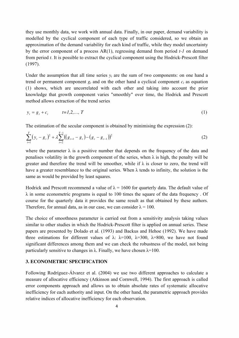
they use monthly data, we work with annual data. Finally, in our paper, demand variability is modelled by the cyclical component of each type of traffic considered, so we obtain an approximation of the demand variability for each kind of traffic, while they model uncertainty by the error component of a process AR(1), regressing demand from period t-1 on demand from period t. It is possible to extract the cyclical component using the Hodrick-Prescott filter (1997).

Under the assumption that all time series yt are the sum of two components: on one hand a trend or permanent component gt and on the other hand a cyclical component ct as equation (1) shows, which are uncorrelated with each other and taking into account the prior knowledge that growth component varies "smoothly" over time, the Hodrick and Prescott method allows extraction of the trend series

ttt cgy t=1,2,…, T (1)

The estimation of the secular component is obtained by minimising the expression (2):

1

2

211

1

2T

t

tttt

T

t

tt gggggy (2)

where the parameter λ is a positive number that depends on the frequency of the data and penalises volatility in the growth component of the series, when λ is high, the penalty will be greater and therefore the trend will be smoother, while if λ is closer to zero, the trend will have a greater resemblance to the original series. When λ tends to infinity, the solution is the same as would be provided by least squares.

Hodrick and Prescott recommend a value of λ = 1600 for quarterly data. The default value of λ in some econometric programs is equal to 100 times the square of the data frequency . Of course for the quarterly data it provides the same result as that obtained by these authors. Therefore, for annual data, as in our case, we can consider λ = 100.

The choice of smoothness parameter is carried out from a sensitivity analysis taking values similar to other studies in which the Hodrick-Prescott filter is applied on annual series. These papers are presented by Dolado et al. (1993) and Backus and Hehoe (1992). We have made three estimations for different values of λ: λ=100, λ=300, λ=800, we have not found significant differences among them and we can check the robustness of the model, not being particularly sensitive to changes in λ. Finally, we have chosen λ=100.

3. ECONOMETRIC SPECIFICATION

Following Rodríguez-Álvarez et al. (2004) we use two different approaches to calculate a measure of allocative efficiency (Atkinson and Cornwell, 1994). The first approach is called error components approach and allows us to obtain absolute rates of systematic allocative inefficiency for each authority and input. On the other hand, the parametric approach provides relative indices of allocative inefficiency for each observation.

5 

 

The calculation of these indices from any of the two methods above mentioned requires, in our case, the estimation of a system of equations formed by an input-oriented distance function and its associated share equations.

The choice of an input oriented distance function, instead of an output oriented distance function, can be justified by the conditions under which port authorities develop their activities, i.e., the authorities do not have control over the volume of traffic which will use their facilities, but they can decide about the inputs that they will use. Therefore, our system of equations is configured as follows:

hhthththt uvTSyxD ,,,ln1ln (3)

ihtiht

iht

hththt

ht

ihtiht Avx

TSyxD

C

wx

ln

),,,(ln (4)

where D(xht,yht,Sht,T) is the short run input distance function, x is an input vector, y is an output vector, S is a quasi-fixed input, and T is the time trend. The subscript h relates to the h-

th port authority and t relates to the time period. The error components vht and viht represent statistical noise, being random disturbance terms distributed with zero mean. The error component uh represents the specific individual effects associated with each authority, which includes technical efficiency as unobservable and time-invariant differences among authorities, but does not contain the cost of allocative efficiency. Finally, the term Aiht represents allocative inefficiencies, represented by the difference between actual and stochastic input cost shares, with uh and Aiht being inherently independent.

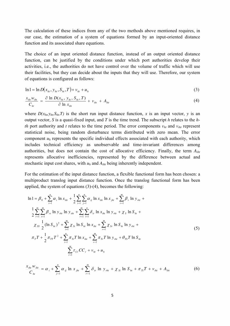
For the estimation of the input distance function, a flexible functional form has been chosen: a multiproduct translog input distance function. Once the translog functional form has been applied, the system of equations (3)-(4), becomes the following:

(5)

(6)

hht

m

r

rCr

htTS

m

r

rhtTr

n

i

ihtTiTTT

m

r

rhthtSr

m

i

ihthtSihtSS

htS

m

r

n

i

rhtihtir

m

r

m

s

shtrhtrs

m

r

rhtr

n

i

n

i

n

j

jhtihtijihti

uvCC

STyTxTTT

ySxSS

Syxyy

yxxx

1

11

2

11

2

1 11 1

11 1 10

lnlnln2

1

lnlnlnln)(ln2

1

lnlnlnlnln2

1

lnlnln2

1ln1ln

ihtihtTihtSirht

m

r

ir

n

j

jhtiji

ht

ihtiht AvTSyxC

wx

lnlnln11

6 

 

.,,,,,,, STTSrTTriTTirSSriSSiriirsrrsjiij

where y = (y1,…,ym) is the output vector , x=(x1,…,xn) is the input vector, S is the quasi-fixed input , CC=(CC1,…CCm) is the cyclical components vector defined in section 2.2 and T is a time trend representing non-neutral technical change. The subscript h=1,…,H relates to the h-

th authority, t relates to the time period and finally, vht and viht represent the statistical noise, uh and Aiht represent individual effects (technical inefficiency) and allocative inefficiency, respectively.

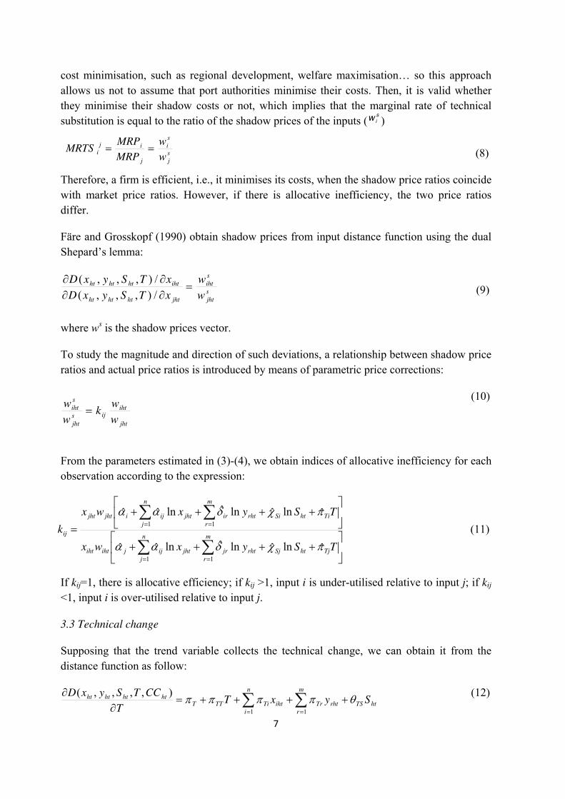
Homogeneity of degree one of the input distance function in variable inputs is enforced by imposing the restrictions:

We also impose the symmetry conditions:

Given that the variables are divided by their geometric means, the first-order coefficients can be interpreted as elasticities at the sample mean

3.1 Error components approach

Allocative efficiency is modelled from of the input cost share equations. The components Aiht are interpreted as a measure of allocative inefficiency which could be systematic given the characteristics of the Spanish port infrastructures. If this inefficient behaviour really occurs, the mean of this component for each authority and input (aih) should be different from zero. Then, equation (4) is transformed as follows:

(7)

where the transformed error terms have zero means.

The coefficients aih can be interpreted as follows: if aih is positive, the input i is being over-utilised with respect to the other inputs, if aih is equal to zero, the input i is being utilised in the optimal proportion, and finally, if aih is negative, the input i is being infra-utilised.

3.2 Parametric approach

Economic theory shows that a firm minimises its costs when the marginal rate of technical substitution of a pair of inputs equals the ratio of their prices. However, in this methodology it is not necessary to assume that firms minimise their real costs. This is interesting because port authorities operate under special conditions which do not necessarily require them to minimise their costs; on one hand, they operate without competition so they have less incentives to be efficient and on the other hand, they may have others objectives apart from

.0,0,0,0,111111

n

i

Ti

n

i

Si

n

i

ir

n

i

ij

n

i

i

)(

lnlnln)(11

ihihtiht

TihtSirht

m

r

ir

n

j

jhtijihi

ht

ihtiht

aAv

TSyxaC

wx

7 

 

jht

ihtijs

jht

s

iht

w

wk

w

w

TSyxwx

TSyxwx

k

TjhtSjrht

m

r

jr

n

j

jhtijjihtiht

TihtSirht

m

r

ir

n

j

jhtijijhtjht

ij

ˆlnˆlnˆlnˆˆ

ˆlnˆlnˆlnˆˆ

11

11

htTS

m

r

rhtTr

n

i

ihtTiTTThthththt SyxT

T

CCTSyxD

11

),,,,(

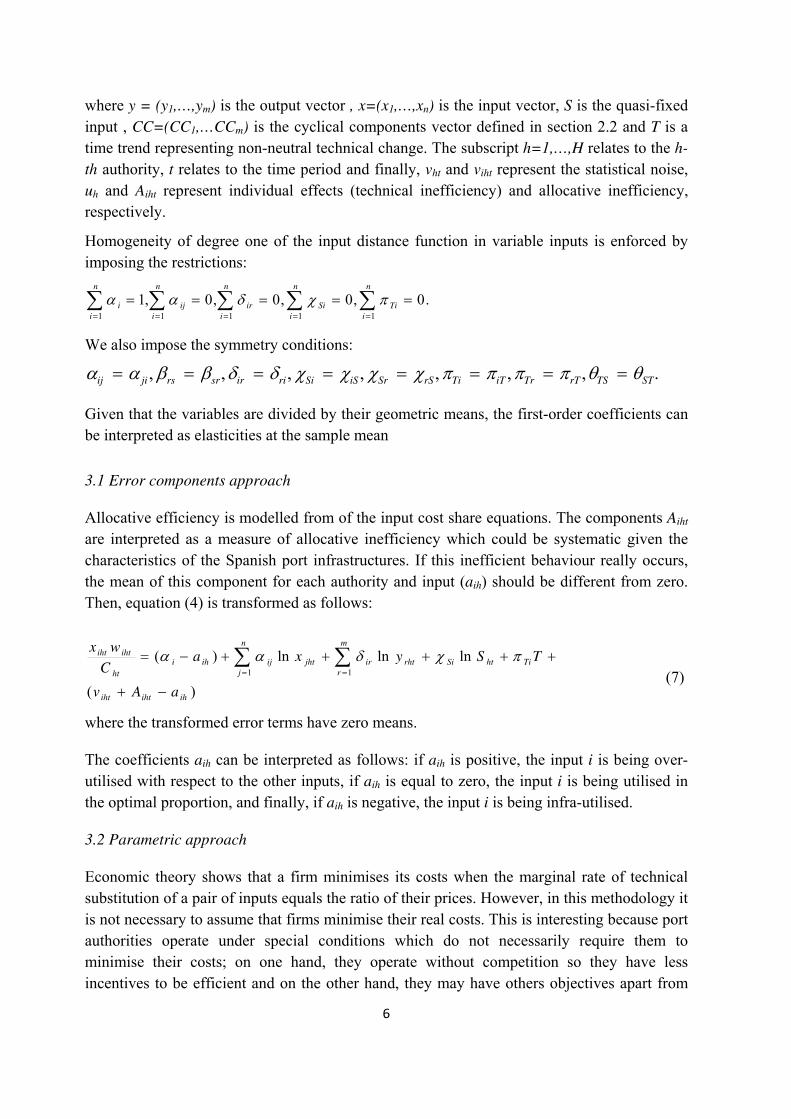
cost minimisation, such as regional development, welfare maximisation… so this approach allows us not to assume that port authorities minimise their costs. Then, it is valid whether they minimise their shadow costs or not, which implies that the marginal rate of technical substitution is equal to the ratio of the shadow prices of the inputs (

s

iw )

(8)

Therefore, a firm is efficient, i.e., it minimises its costs, when the shadow price ratios coincide with market price ratios. However, if there is allocative inefficiency, the two price ratios differ.

Färe and Grosskopf (1990) obtain shadow prices from input distance function using the dual Shepard’s lemma:

(9)

where ws is the shadow prices vector.

To study the magnitude and direction of such deviations, a relationship between shadow price ratios and actual price ratios is introduced by means of parametric price corrections:

(10)

From the parameters estimated in (3)-(4), we obtain indices of allocative inefficiency for each observation according to the expression:

(11)

If kij=1, there is allocative efficiency; if kij >1, input i is under-utilised relative to input j; if kij <1, input i is over-utilised relative to input j.

3.3 Technical change

Supposing that the trend variable collects the technical change, we can obtain it from the distance function as follow:

(12)

s

j

s

i

j

ij

iw

w

MRP

MRPMRTS

s

jht

s

iht

jhthththt

ihthththt

w

w

xTSyxD

xTSyxD

/),,,(

/),,,(

8 

 

n

i

ihtTi x1

TTTT

m

r

rhtTr y1

STS

In equation (12) we can identify four components of technical change (Baltagi and Griffin, 1988; Bhattacharyya and Mitra, 1997):

Pure technological change (PTC),

Non-neutral technological change (NTC),

Scale-augmenting technological change (STC),

Quasi-fixed factor augmenting technological change

The first component represents the neutral technological change, which does not affect the use of factor and the degree of scale economies. The second term includes the effect of technological change on the inputs participations, so a positive sign of Ti implies that technological change is intensive in the use of input i, while a negative value means that technological progress is saved on input i. The third component is the impact of technological change on the economies of scale, a positive value of this term suggests that size elasticity, and therefore the minimum efficient scale, increases with time, so authorities can take advantage of greater economies of scale. Finally, the fourth component shows the effect of technological change on the quasi-fixed factor.

4. DATA DESCRIPTION

The sample consists of 27 Spanish port authorities which manage 46 ports. For these ports, annual data from 1986 until 2007 are available, being the complete panel data set of 594 observations3.

The data were gathered from the annual reports of Puertos del Estado (several years). This information has been used in other studies such as Coto-Millán et al. (2000), Baños-Pino et al. (1999), González and Trujillo (2008), Martínez-Budría et al. (1999), Núñez-Sánchez et al. (2011), etc.

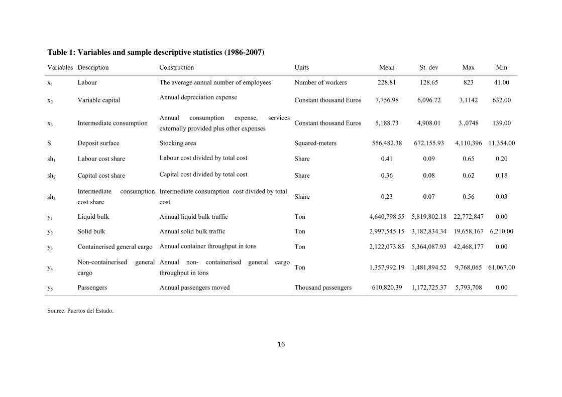
Port activity is multiproduct and for this reason we have taken into account five outputs: Liquid bulk (y1), Solid bulk (y2), Containerised general cargo (y3), Non-containerised general cargo (y4) and Passengers (y5). We also include three variable inputs: Labour (x1), Variable capital (x2) and Intermediate consumption (x4). Finally, a quasi-fixed input is defined in the specification of the distance function: Deposit surface (S), input cost shares and the cyclical components of traffics. Table 1 shows the variables, their construction and their descriptive statistics.

INSERT TABLE 1 HERE

5. ESTIMATION AND RESULTS

                                                            3 It is necessary to point out that the authorities of Almería and Motril are separated since 2005. However, in order to simplify the analysis, we have considered both authorities as a unit during the entire sample period.

9 

 

In order to avoid endogeneity problems for the inputs, the system of equations (5)-(6) has been estimated using instrumental variables (Iterated Three-Stage Least Squares), which is equivalent to maximum likelihood estimation. Since the analysis focuses only on the provision of port infrastructure, outputs are not considered endogenous as agents that have some power over where o when cargo will be moved are port terminals, so we consider that port authorities just have control over the inputs that they contract. The instruments used are the input variables lagged one period. This analysis focuses only on the provision of port infrastructure, therefore outputs are not considered endogenous since port authorities do not have control over them. We assume that this control belongs to the port terminals and shipping companies who decide where the freight will be moved.

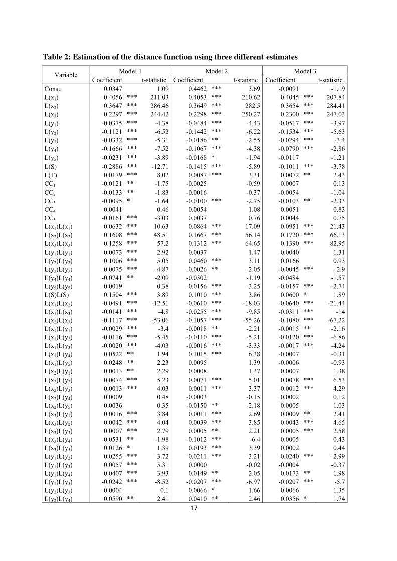
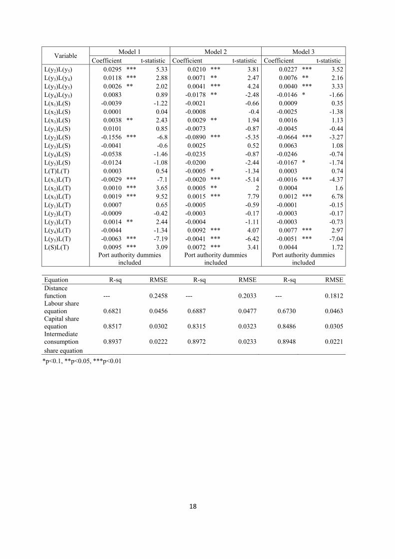
Table 2 shows the results of the estimation using three different models. First, the system of equations has been estimated using pooled data (model 1). This specification does not distinguish among the port authorities which form the data panel, so it cannot collect the presence of unobserved heterogeneity. In this way, not taking into account this heterogeneity may lead to biased estimations. The second specification for estimation corresponds to a fixed effect estimation where unobserved heterogeneity is collected by the inclusion of a set of dummies which represent the effect of time-invariant individual characteristics of each port authority. This model is the most appropriate when unobserved heterogeneity is correlated with the regressors used in the specification if this correlation does not exist, a random effects model would provide more efficient estimations than the fixed effects one. In this way, model 3 presents the specification of a random effects estimator. Therefore, if there is no correlation among unobserved heterogeneity and regressors, both models (model 2 and 3) give us consistent estimations, but model 3 would be the most efficient. If that correlation occurs, model 3 would be inconsistent and therefore model 2 is the right one.

In order to analyse the validity of model 1, test it is tested against model 2 using a Wald test. If the test rejects the null hypothesis, model 2 is more appropriate than model 1, if we cannot reject the hypothesis, model 1 would be chosen. The result obtained provides empirical evidence for rejecting the pooled model. Once model 1 has been rejected, the choice between model 2 and model 3 has been carried out by a Hausman test: if this contrast leads us not to reject the null hypothesis, it means that the difference between both estimators is very small, so we should choose the most efficient one, i.e., the random effects estimator, if instead the test reject the null hypothesis, the fixed effect model should be chosen. The Hausman test result leads us to reject the null hypothesis and therefore the model that best fits the characteristics of the sample is the fixed effects model. In this way we find evidence that unobserved heterogeneity of the port authority is correlated with the regressors included in the specification.

INSERT TABLE 2

From the estimation of model 2 we can see that, at the sample mean, the regularity conditions are satisfied: it is non-decreasing and quasi-concave in variable inputs, decreasing in outputs

10 

 

and homogeneous of degree one in variable inputs. Moreover, we have tested whether the technology underlying the estimated distance function is homothetic and Wald test statistics lead us to reject this hypothesis. Therefore, we can conclude that the proportions of inputs used for port authorities depend on the level of output.

Table 2 shows that every first-order coefficient is statistically significant and has the expected sign. The parameters of variable inputs are positive and, thus, indicate that distance from the limit increases when the use of input grows. On the other hand, output parameters are negative, evidencing that if outputs increase, the distance will be reduced. The sum of the first-order output parameters is less than one in absolute value, indicating the presence of increasing returns to scale. Moreover, we can conclude that labour presents a higher elasticity than the rest of variable inputs and that elasticity of non-containerised general cargo is the highest in relation with the other elasticities related to outputs.

We also find evidence of the existence of technological progress since the coefficient associated to the trend is positive and significant. The results also show that this technical progress is labour-saving while increasing the use of capital and intermediate consumption. Furthermore, if we take into account the scale effect on technological change, we can see that the coefficients of the trend iterations with only two products are statistically different from zero. These are non-containerised general cargo and passengers. In the first case, the parameter is positive which means that there has been technical progress. Such progress in the case of port authorities could translate into savings of space. Therefore port authorities could supply more of this commodity with a lower increase in costs due to the use of new economies of scale. By contrast, in the other case, the coefficient related to passengers is negative which means that the effects of this traffic on the production process of the authorities are becoming worse over time. If we add the six parameters of these iterations, the result is very close to zero, which means that the efficiency scale has not changed. Finally, the effect of technological change on the quasi-fixed input is positive which means the use of this input improves over this period.

On the other hand, the deposit area coefficient is negative and statistically significant, which means that the marginal productivity of deposit area is negative. This result could be partially explained due to the fact that port authorities have more deposit area than previously needed (Rodríguez-Álvarez et al. 2007).

The coefficients of the cyclical components are all non-significant except the cyclical component of containerised general cargo4. This is a logical result, given that this type of traffic has become the most important traffic in recent decades and maybe the most desirable for port authorities, showing a dramatic growth because it is the most efficient and cheapest traffic, being also highly competitive. A negative sign in its coefficient means that the variability has a negative effect on the productivity of port authorities. From the duality

                                                            4 This result may be due to the structure of the data. If instead of having annual data, monthly or even quarterly data were available, demand variability would be clearer, since shipping traffic has a highly seasonal component.

11 

 

rr

rCC

C

CC

TSCCxyDMCCC

ln

),,,,(ln

between distance function and cost function we can obtain the marginal cost of containerised general cargo traffic variability.

r = 1,…,m (13)

where C is the total cost. Given that only the effect of the cyclical component of containerised general cargo is nonzero at the usual confidence levels, its marginal cost is the most important. Therefore, from equation (13) we can conclude that, at the mean, a percentage increase of 1% in this cyclical component causes, ceteris paribus, an increase of 0.051% in variable costs.

As mentioned above, the inclusion of the cyclical components of the traffics seems not to have an effect on the production process of the port authorities, with the exception of containerised general cargo, so we may infer that demand variability is not the major cause of excess of capacity. Probably, others factors such as competition with the nearest ports, the Averch-Johnson effect linked to the rate of return regulation, or vertical relationships with other ports operators may have a greater weight than the uncertainty when port authorities make investment decisions on capacity.

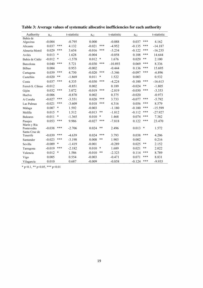
From the estimation of the system of equations it is also possible to obtain the allocative efficiency indices mentioned in Section 4. Allocative efficiency indices estimated by error components approach are shown in Table 3. These parameters represent the existing systematic allocative inefficiency over the sample period for each input and port authority.

INSERT TABLE 3

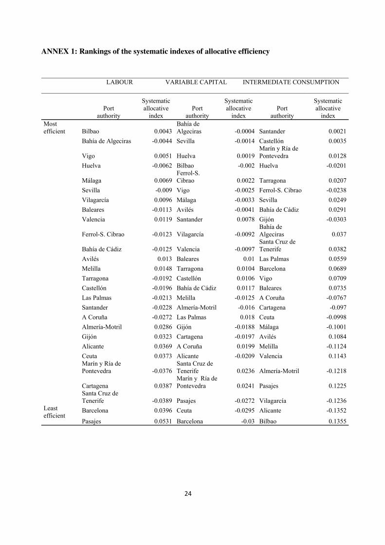
The authorities from Bahía de Algeciras, Bilbao, Ferrol-S.Cibrao, Huelva, Vigo and Vilagarcía are allocative efficient in the use of variable capital and labour, whereas Avilés, Sevilla and Málaga only use the variable capital in the correct way. The remaining authorities use these inputs in an inefficient way, they over-utilise these inputs when the indices are greater than zero and vice versa. The intermediate consumptions are inefficiently allocated by all authorities except Castellón, Huelva and Santander5.

Table 3 shows that those authorities located on islands follow a common pattern. At the mean, they tend to under-utilise the labour and over-use the variable capital, while in the case of Ceuta and Melilla both over-use the labour input and under-use the variable capital.

Annex I shows the rankings of the systematic allocative efficiency for each input.

As already mentioned, these indices allow us to measure the systematic or time invariant allocative inefficiency in which port authorities incur during the development of their productive activity, while the parametric approach allows us to obtain relative indices of

                                                            5 This result may be due to the construction of the variable which encompasses all supplies, external services… forming a heterogeneous group.

12 

 

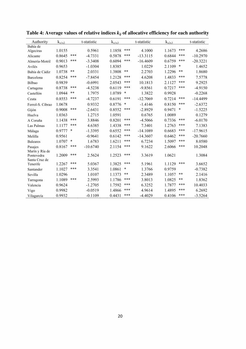
allocative efficiency (kij) for observation. Table 4 shows the average indices for each port authority. It is important to remember that a kij coefficient greater than one indicates that the factor i is being underutilised with respect to factor j and vice versa, and therefore t-statistics in Table 4 test if the parameter kij is equal or different to one by a test of means.

INSERT TABLE 4

From Table 4 we can see that port authorities from Cadiz, Castellón, A Coruña, Las Palmas, Baleares, Pontevedra, Santa Cruz de Tenerife, Santander and Tarragona underuse labour with respect to variable capital. On the opposite side, Alicante, Almeria, Barcelona, Cartagena, Ceuta, Gijón, Málaga and Pasajes overuse labour with respect to variable capital. The remaining port authorities are efficient in their use of these inputs. When we introduce the intermediate consumption in the estimation of these indices the number of efficient port authorities is reduced. In the case of the relation between labour and intermediate consumption, just Avilés and Huelva are efficient while Bahía de Algeciras, Cadiz, Barcelona, Bilbao, Castellón, Las Palmas, Baleares, Pasajes, Pontevedra, Santa Cruz de Tenerife, Santander, Sevilla, Tarragona, Valencia and Vigo underused labour with respect to intermediate consumption, the remaining authorities behaved in the opposite manner. Finally, in terms of proportion in the use of variable capital relative to intermediate consumption, the authorities from Castellón, Huelva, Pontevedra and Santander are efficient in an allocative way, while Bahía de Algeciras, Aviles, Cadiz, Barcelona, Bilbao, Las Palmas, Baleares, Pasajes, Santa Cruz de Tenerife, Sevilla, Tarragona, Valencia and Vigo, on average, underuse the capital with respect to intermediate consumption, otherwise occurring in the other authorities.

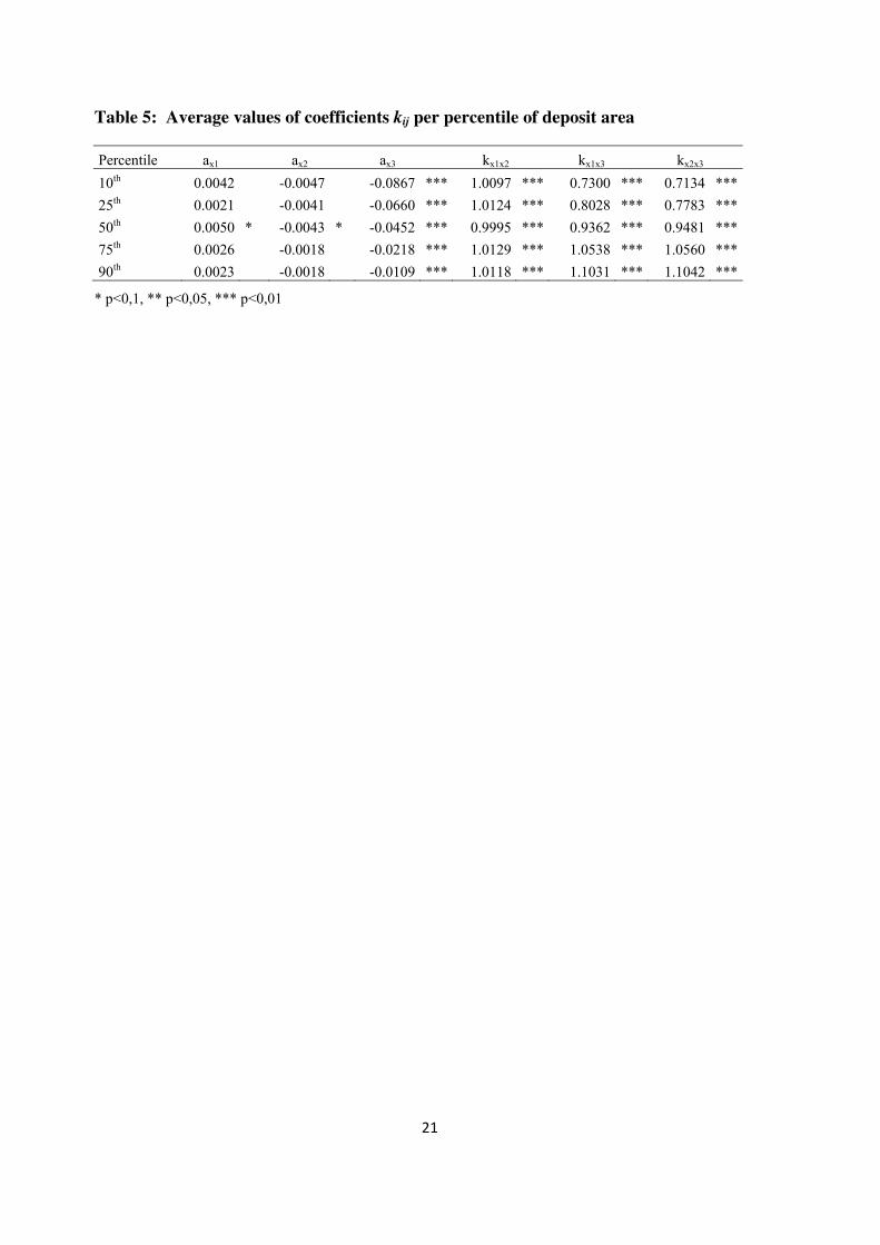
Table 5 reports the average values of the efficiency indices (systematic and relative) for different percentiles of the deposit area variable. It shows that the levels of systematic allocative efficiency for intermediate consumption improve with increasing deposit area. In the case of labour and capital, the systematic indices indicate an efficient behaviour regardless of the area in all percentiles except the 50th one, so we can conclude that there is not a relevant relation between these indices and the deposit area. In the case of the indices obtained from the parametric approach, the index which links labour and capital does not show a clear relation between kx1x2 and deposit area while the indices which relate intermediate consumption with the other variable inputs improve with the area size until the 90th, in which they become worse. Thus we can conclude that the inefficiency levels increase when the largest authorities are included in the percentile, although without reaching the levels of the first percentiles.

INSERT TABLE 5

The results show that the proportions in which the variable inputs are used are not optimal in most cases, and therefore costs would be reduced by improving the levels of allocative efficiency. For that to occur, it is important to determine whether variable inputs would be

13 

 

adequate substitutes. From the estimated distance function it is possible to analyse the degree of substitutability among variable inputs by means of Morishima substitution elasticities .

These elasticities inform about the variations of shadow prices given a variation in the input quantity. Positive values indicate complementarity between inputs while negative values represent substitutability. Morishima elasticities are divided into two components: on one hand, the cross-price elasticity shadow (Eij) which tell us if the input pairs are net substitutes or net complementaries, and on the other hand, the elasticity price (Eii). These elasticities are formally defined as follows:

(15)

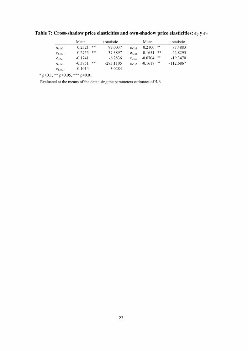
The results from the estimation of Morishima elasticities and their components are show in Tables 6 and 7. These results indicate that there is little scope for substitution between different pairs of inputs which, according to Rodríguez-Álvarez et al. (2004), implies that resolving allocative inefficiency is a difficult task. The estimated values of the shadow price elasticities have the expected sign for all inputs. The estimation of the cross-shadow price elasticities shows that labour is a net complementary input with variable capital and intermediate consumption, with the value of the cross-shadow price elasticity for variable capital and intermediate consumptions not being significant. Finally, the estimation of Morishima elasticities shows that labour is complementary with variable capital and intermediate consumption, confirming the results obtained previously. On the other hand, the Morishima elasticity between variable capital and intermediate consumption is not statistically significant.

INSERT TABLE 6

INSERT TABLE 7

6. CONCLUSIONS

This paper is an empirical application of a system of equations formed by an input distance function and cost share equations in order to assess the allocative inefficiency in which Spanish port authorities incur in the development of their economic activity. From this system of equations it is possible to estimate two different measures of allocative efficiency using two approaches: on one hand, the error components approach provides an absolute measure of systematic allocative inefficiency for each authority and input. On the other hand, the parametric approach allows obtaining relative indices of allocative inefficiency between pair of inputs for each observation. Our paper is the first one modelling demand variability using the cyclical component of the traffics in order to include estimations of uncertainty as explanatory variables in the distance function. The cyclical component of the traffic series has been extracted applying the Hodrick-Presscot filter. Moreover, from the duality between the

),(),(

),(/),(),(/),(

xyExyE

xyDxyDxxyDxyDx

iiij

iiiijiji

jijjiiij xxdxxyDxxyDdxyM /ln//,(/)/,(ln),(

14 

 

distance function and cost function, we have estimated the marginal cost associated with the uncertainty.

This empirical model has been applied to a panel of data formed by 27 Spanish port authorities during the period 1986-2007. The sample period has been characterised by an important growth of maritime traffic and several regulatory changes which have led these authorities to be managed by a landlord model and operate according to principles such as financial and operating autonomy, competence, quality and efficiency, with a growing participation of the private sector in port activities.

The main results of the paper are: first, we have found empirical evidence of the existence of increasing returns to scale and non-neutral technological progress. Second, after the inclusion of demand variability estimations as explanatory variables, only the cyclical component of containerised general cargo is significant at the usual confidence levels. This makes sense because this kind of traffic is the most competitive and volatile. Third, the marginal productivity of deposit area is negative due to the existence of an excess of capacity. From this and the former results, we conclude that demand variability is not the main reason for the excess of capacity; other factors such as regulation (Averch-Johnson effect), competition between nearest ports or vertical relationships among port operators may be more important determinants than uncertainty on the investment decisions on capacity. Our model is not prepared to discuss what the effect of these factors on investment decisions is, but it could be a good starting point for future research. Finally, it has been found that resource allocation is not efficient. Moreover, the estimations of Morishima elasticities show that the possibilities of substitution between pairs of inputs are very limited, so the allocative inefficiencies in the Spanish port system are difficult to solve in the short term.

REFERENCES

Atkinson SE, Cornwell C (1994) Parametric estimation of technical and allocative inefficiency with panel data. Int Econ Rev 35(1): 231-243.

Backus D, Kehoe P (1992) International evidence on the historical properties of business cycles. Am Econ Rev 82 (4): 864-888.

Baltagi BH, Griffin JM (1988) A general index of technical change. J of Polit Econ 96: 20-41.

Baños-Pino J, Coto-Millán P, Rodríguez-Álvarez A (1999) Allocative efficiency and overcapitalization: An application. Int J of Transp Econ XXVI(2): 181-199.

Bhattacharyya A, Mitra K (1997) Decomposition of technological change and factor bias in Indian power sector: An unbalanced panel data approach. J of Prod Anal 8: 35-52.

Coto-Millán P, Baños-Pino J, Rodríguez-Álvarez A. (2000) Economic efficiency in Spanish ports: Some empirical evidence. Marit Policy and Manag 27(2): 169-174.

15 

 

Dolado J, Sebastián M, Vallés J (1993) Cyclical patterns of the Spanish economy. Banco de España. Working paper nº 9324.

Färe R, Grosskopf S. (1990). A distance function approach to price efficiency. J of Public Econ 43: 123-126.

Gaynor M, Anderson GF (1995) Uncertain demand, the structure of hospital costs, and the cost of empty hospital beds. J of Health Econ 14: 291-317.

González MM, Trujillo L (2008) Reforms and infraestructure efficiency in Spain’s container ports. Transp Res A 42: 243-257.

Hodrick RJ, Prescott EC (1997) Postwar U.S. business cycles: An empirical investigation. J of Money, Credit, and Bank 29(1): 1-16.

Martínez-Budría E, Díaz-Armas R, Navarro-Ibáñez M, Ravelo-Mesa T (1999) A study of the efficiency of Spanish port authorities using data envelopment analysis. International J of Trans Econ XXVI (2): 237-253.

Nuñez-Sánchez R., Jara-Díaz S., Coto-Millán P. (2011) Public regulation and passengers importance in port infrastructure costs. Transp Res A, 45: 653-666.

Puertos del Estado (several years) Anuario estadístico, Ministerio de Fomento, Madrid.

Rodríguez-Álvarez A, Fernández-Blanco V, Knox Lovell CA (2004) Allocative inefficiency and its costs: The case of Spanish public hospitals. International J of Prod Econ 92: 99-111.

Rodríguez-Álvarez A, Tovar B, Trujillo L (2007) Firm and time varying technical and allocative efficiency: An application to port cargo handling firms. Int J of Prod Econ 109: 146-161.

Rodríguez-Álvarez A, Tovar B, Wall A (2011) The effect of demand uncertainty on port terminal costs. J Transp Econ Policy 45(2): 303-328.

Tovar B, Wall A (2010) Economies of scale and scope in service firms with demand uncertain: An application to a Spanish port. Fundación de las Cajas de Ahorros. Working paper No 565/2010.

16 

 

Table 1: Variables and sample descriptive statistics (1986-2007)

Variables Description Construction Units Mean St. dev Max Min

x1 Labour The average annual number of employees Number of workers 228.81 128.65 823 41.00

x2 Variable capital Annual depreciation expense Constant thousand Euros 7,756.98 6,096.72 3,1142 632.00

x3 Intermediate consumption Annual consumption expense, services

externally provided plus other expenses Constant thousand Euros 5,188.73 4,908.01 3.,0748 139.00

S Deposit surface Stocking area Squared-meters 556,482.38 672,155.93 4,110,396 11,354.00

sh1 Labour cost share Labour cost divided by total cost Share 0.41 0.09 0.65 0.20

sh2 Capital cost share Capital cost divided by total cost Share 0.36 0.08 0.62 0.18

sh3 Intermediate consumption

cost share

Intermediate consumption cost divided by total

cost Share 0.23 0.07 0.56 0.03

y1 Liquid bulk Annual liquid bulk traffic Ton 4,640,798.55 5,819,802.18 22,772,847 0.00

y2 Solid bulk Annual solid bulk traffic Ton 2,997,545.15 3,182,834.34 19,658,167 6,210.00

y3 Containerised general cargo Annual container throughput in tons Ton 2,122,073.85 5,364,087.93 42,468,177 0.00

y4 Non-containerised general

cargo

Annual non- containerised general cargo

throughput in tons Ton 1,357,992.19 1,481,894.52 9,768,065 61,067.00

y5 Passengers Annual passengers moved Thousand passengers 610,820.39 1,172,725.37 5,793,708 0.00

Source: Puertos del Estado.

17 

 

Table 2: Estimation of the distance function using three different estimates

Variable Model 1 Model 2 Model 3

Coefficient t-statistic Coefficient t-statistic Coefficient t-statistic Const. 0.0347 1.09 0.4462 *** 3.69 -0.0091 -1.19L(x1) 0.4056 *** 211.03 0.4053 *** 210.62 0.4045 *** 207.84L(x2) 0.3647 *** 286.46 0.3649 *** 282.5 0.3654 *** 284.41L(x3) 0.2297 *** 244.42 0.2298 *** 250.27 0.2300 *** 247.03L(y1) -0.0375 *** -4.38 -0.0484 *** -4.43 -0.0517 *** -3.97L(y2) -0.1121 *** -6.52 -0.1442 *** -6.22 -0.1534 *** -5.63L(y3) -0.0332 *** -5.31 -0.0186 ** -2.55 -0.0294 *** -3.4L(y4) -0.1666 *** -7.52 -0.1067 *** -4.38 -0.0790 *** -2.86L(y5) -0.0231 *** -3.89 -0.0168 * -1.94 -0.0117 -1.21L(S) -0.2886 *** -12.71 -0.1415 *** -5.89 -0.1011 *** -3.78L(T) 0.0179 *** 8.02 0.0087 *** 3.31 0.0072 ** 2.43CC1 -0.0121 ** -1.75 -0.0025 -0.59 0.0007 0.13CC2 -0.0133 ** -1.83 -0.0016 -0.37 -0.0054 -1.04CC3 -0.0095 * -1.64 -0.0100 *** -2.75 -0.0103 ** -2.33CC4 0.0041 0.46 0.0054 1.08 0.0051 0.83CC5 -0.0161 *** -3.03 0.0037 0.76 0.0044 0.75L(x1)L(x1) 0.0632 *** 10.63 0.0864 *** 17.09 0.0951 *** 21.43L(x2)L(x2) 0.1608 *** 48.51 0.1667 *** 56.14 0.1720 *** 66.13L(x3)L(x3) 0.1258 *** 57.2 0.1312 *** 64.65 0.1390 *** 82.95L(y1)L(y1) 0.0073 *** 2.92 0.0037 1.47 0.0040 1.31L(y2)L(y2) 0.1006 *** 5.05 0.0460 *** 3.11 0.0166 0.93L(y3)L(y3) -0.0075 *** -4.87 -0.0026 ** -2.05 -0.0045 *** -2.9L(y4)L(y4) -0.0741 ** -2.09 -0.0302 -1.19 -0.0484 -1.57L(y5)L(y5) 0.0019 0.38 -0.0156 *** -3.25 -0.0157 *** -2.74L(S)L(S) 0.1504 *** 3.89 0.1010 *** 3.86 0.0600 * 1.89L(x1)L(x2) -0.0491 *** -12.51 -0.0610 *** -18.03 -0.0640 *** -21.44L(x1)L(x3) -0.0141 *** -4.8 -0.0255 *** -9.85 -0.0311 *** -14L(x2)L(x3) -0.1117 *** -53.06 -0.1057 *** -55.26 -0.1080 *** -67.22L(x1)L(y1) -0.0029 *** -3.4 -0.0018 ** -2.21 -0.0015 ** -2.16L(x1)L(y2) -0.0116 *** -5.45 -0.0110 *** -5.21 -0.0120 *** -6.86L(x1)L(y3) -0.0020 *** -4.03 -0.0016 *** -3.33 -0.0017 *** -4.24L(x1)L(y4) 0.0522 ** 1.94 0.1015 *** 6.38 -0.0007 -0.31L(x1)L(y5) 0.0248 ** 2.23 0.0095 1.39 -0.0006 -0.93L(x2)L(y1) 0.0013 ** 2.29 0.0008 1.37 0.0007 1.38L(x2)L(y2) 0.0074 *** 5.23 0.0071 *** 5.01 0.0078 *** 6.53L(x2)L(y3) 0.0013 *** 4.03 0.0011 *** 3.37 0.0012 *** 4.29L(x2)L(y4) 0.0009 0.48 -0.0003 -0.15 0.0002 0.12L(x2)L(y5) 0.0036 0.35 -0.0150 ** -2.18 0.0005 1.03L(x3)L(y1) 0.0016 *** 3.84 0.0011 *** 2.69 0.0009 ** 2.41L(x3)L(y2) 0.0042 *** 4.04 0.0039 *** 3.85 0.0043 *** 4.65L(x3)L(y3) 0.0007 *** 2.79 0.0005 ** 2.21 0.0005 *** 2.58L(x3)L(y4) -0.0531 ** -1.98 -0.1012 *** -6.4 0.0005 0.43L(x3)L(y5) 0.0126 * 1.39 0.0193 *** 3.39 0.0002 0.44L(y1)L(y2) -0.0255 *** -3.72 -0.0211 *** -3.21 -0.0240 *** -2.99L(y1)L(y3) 0.0057 *** 5.31 0.0000 -0.02 -0.0004 -0.37L(y1)L(y4) 0.0407 *** 3.93 0.0149 ** 2.05 0.0173 ** 1.98L(y1)L(y5) -0.0242 *** -8.52 -0.0207 *** -6.97 -0.0207 *** -5.7L(y2)L(y3) 0.0004 0.1 0.0066 * 1.66 0.0066 1.35L(y2)L(y4) 0.0590 ** 2.41 0.0410 ** 2.46 0.0356 * 1.74

18 

 

Variable Model 1 Model 2 Model 3

Coefficient t-statistic Coefficient t-statistic Coefficient t-statistic L(y2)L(y5) 0.0295 *** 5.33 0.0210 *** 3.81 0.0227 *** 3.52L(y3)L(y4) 0.0118 *** 2.88 0.0071 ** 2.47 0.0076 ** 2.16L(y3)L(y5) 0.0026 ** 2.02 0.0041 *** 4.24 0.0040 *** 3.33L(y4)L(y5) 0.0083 0.89 -0.0178 ** -2.48 -0.0146 * -1.66L(x1)L(S) -0.0039 -1.22 -0.0021 -0.66 0.0009 0.35L(x2)L(S) 0.0001 0.04 -0.0008 -0.4 -0.0025 -1.38L(x3)L(S) 0.0038 ** 2.43 0.0029 ** 1.94 0.0016 1.13L(y1)L(S) 0.0101 0.85 -0.0073 -0.87 -0.0045 -0.44L(y2)L(S) -0.1556 *** -6.8 -0.0890 *** -5.35 -0.0664 *** -3.27L(y3)L(S) -0.0041 -0.6 0.0025 0.52 0.0063 1.08L(y4)L(S) -0.0538 -1.46 -0.0235 -0.87 -0.0246 -0.74L(y5)L(S) -0.0124 -1.08 -0.0200 -2.44 -0.0167 * -1.74L(T)L(T) 0.0003 0.54 -0.0005 * -1.34 0.0003 0.74L(x1)L(T) -0.0029 *** -7.1 -0.0020 *** -5.14 -0.0016 *** -4.37L(x2)L(T) 0.0010 *** 3.65 0.0005 ** 2 0.0004 1.6L(x3)L(T) 0.0019 *** 9.52 0.0015 *** 7.79 0.0012 *** 6.78L(y1)L(T) 0.0007 0.65 -0.0005 -0.59 -0.0001 -0.15L(y2)L(T) -0.0009 -0.42 -0.0003 -0.17 -0.0003 -0.17L(y3)L(T) 0.0014 ** 2.44 -0.0004 -1.11 -0.0003 -0.73L(y4)L(T) -0.0044 -1.34 0.0092 *** 4.07 0.0077 *** 2.97L(y5)L(T) -0.0063 *** -7.19 -0.0041 *** -6.42 -0.0051 *** -7.04L(S)L(T) 0.0095 *** 3.09 0.0072 *** 3.41 0.0044 1.72

Port authority dummies

included Port authority dummies

included Port authority dummies

included Equation R-sq RMSE R-sq RMSE R-sq RMSEDistance function --- 0.2458 --- 0.2033 --- 0.1812Labour share equation 0.6821 0.0456 0.6887 0.0477 0.6730 0.0463Capital share equation 0.8517 0.0302 0.8315 0.0323 0.8486 0.0305Intermediate consumption 0.8937 0.0222 0.8972 0.0233 0.8948 0.0221share equation

*p<0.1, **p<0.05, ***p<0.01

19 

 

Table 3: Average values of systematic allocative inefficiencies for each authority

Authority ax1 t-statistic ax2 t-statistic ax3 t-statistic Bahía de Algeciras -0.004 -0.795 0.000 -0.088 0.037 *** 4.162 Alicante 0.037 *** 4.132 -0.021 *** -4.952 -0.135 *** -14.187 Almería-Motril 0.029 *** 3.654 -0.016 *** -3.234 -0.122 *** -16.235 Avilés 0.013 * 1.628 -0.004 -0.858 0.108 *** 14.644 Bahía de Cádiz -0.012 * -1.578 0.012 * 1.676 0.029 ** 2.100

Barcelona 0.040 *** 5.721 -0.030 *** -10.893 0.069 *** 8.336 Bilbao 0.004 0.953 -0.002 -0.444 0.136 *** 15.695 Cartagena 0.039 *** 4.750 -0.020 *** -3.346 -0.097 *** -6.896 Castellón -0.020 ** -1.869 0.011 * 1.522 0.003 0.532 Ceuta 0.037 *** 4.335 -0.030 *** -4.224 -0.100 *** -16.613 Ferrol-S. Cibrao -0.012 -0.851 0.002 0.189 -0.024 ** -1.805 Gijón 0.032 *** 3.072 -0.019 *** -2.819 -0.030 *** -3.353 Huelva -0.006 -0.870 0.002 0.375 -0.020 -0.973 A Coruña -0.027 *** -3.551 0.020 *** 3.733 -0.077 *** -5.792 Las Palmas -0.021 *** -3.609 0.018 *** 4.316 0.056 *** 8.579 Málaga 0.007 * 1.592 -0.003 -1.180 -0.100 *** -15.599 Melilla 0.015 * 1.512 -0.013 ** -1.812 -0.112 *** -27.927 Baleares -0.011 * -1.365 0.010 * 1.468 0.074 *** 7.382 Pasajes 0.053 *** 9.986 -0.027 *** -7.818 0.122 *** 23.470 Marín y Ría Pontevedra -0.038 *** -2.706 0.024 ** 2.496 0.013 * 1.572 Santa Cruz de Tenerife -0.039 *** -4.639 0.024 *** 3.793 0.038 *** 4.206 Santander -0.023 *** -3.198 0.008 ** 1.903 0.002 0.216 Sevilla -0.009 * -1.419 -0.001 -0.289 0.025 ** 2.152 Tarragona -0.019 *** -2.182 0.010 * 1.689 0.021 ** 2.022 Valencia 0.012 * 1.586 -0.010 ** -2.323 0.114 *** 8.789 Vigo 0.005 0.554 -0.003 -0.471 0.071 *** 8.831 Vilagarcía 0.010 0.687 -0.009 -0.858 -0.124 *** -9.935

* p<0.1, ** p<0.05, *** p<0.01

20 

 

Table 4: Average values of relative indices kij of allocative efficiency for each authority

Authority kx1x2 t-statistic kx1x3 t-statistic kx2x3 t-statistic Bahía de Algeciras 1.0155 0.5961 1.1858 *** 4.1000 1.1673 *** 4.2686Alicante 0.8645 *** -4.7331 0.5878 *** -13.3115 0.6844 *** -10.2970Almería-Motril 0.9013 *** -3.3408 0.6094 *** -16.4609 0.6759 *** -20.3221Avilés 0.9653 -1.0304 1.8385 1.0229 2.1109 * 1.4652Bahía de Cádiz 1.0738 ** 2.0331 1.3808 ** 2.2703 1.2296 ** 1.8680

Barcelona 0.8254 *** -7.8454 1.2128 *** 4.6208 1.4833 *** 7.5778Bilbao 0.9839 -0.6991 2.0543 *** 10.1813 2.1127 *** 9.2925Cartagena 0.8738 *** -4.5238 0.6119 *** -9.8561 0.7217 *** -4.9150Castellón 1.0944 ** 1.7975 1.0789 * 1.3822 0.9928 -0.2268Ceuta 0.8553 *** -4.7237 0.6191 *** -12.7069 0.7214 *** -14.4499Ferrol-S. Cibrao 1.0678 0.9332 0.8776 * -1.4146 0.8150 *** -2.6372Gijón 0.9008 *** -2.6431 0.8552 *** -2.8929 0.9471 * -1.5225Huelva 1.0363 1.2715 1.0591 0.6765 1.0089 0.1279A Coruña 1.1438 *** 3.8846 0.8201 *** -4.5066 0.7336 *** -6.0170Las Palmas 1.1177 *** 4.6385 1.4338 *** 7.3401 1.2763 *** 7.1383Málaga 0.9777 * -1.3395 0.6552 *** -14.1089 0.6683 *** -17.9615Melilla 0.9561 -0.9641 0.6142 *** -14.3607 0.6462 *** -20.7660Baleares 1.0707 * 1.6783 1.6211 *** 6.7234 1.5097 *** 8.0580Pasajes 0.8167 *** -10.6740 2.1154 *** 9.1622 2.6066 *** 10.2048Marín y Ría de Pontevedra 1.2009 *** 2.5624 1.2523 *** 3.3619 1.0621 1.3084Santa Cruz de Tenerife 1.2267 *** 5.0367 1.3825 *** 5.1961 1.1129 *** 3.6652Santander 1.1027 *** 3.3541 1.0861 * 1.3766 0.9759 -0.7382Sevilla 1.0296 1.0107 1.1373 ** 2.3489 1.1057 ** 2.1416Tarragona 1.1089 *** 2.5993 1.1786 *** 3.8013 1.0825 ** 1.8362Valencia 0.9624 -1.2705 1.7592 *** 6.3252 1.7877 *** 10.4033Vigo 0.9982 -0.0519 1.4866 *** 4.9614 1.4895 *** 6.2692Vilagarcía 0.9932 -0.1109 0.4431 *** -4.4029 0.4106 *** -3.5264

21 

 

Table 5: Average values of coefficients kij per percentile of deposit area

Percentile ax1 ax2 ax3 kx1x2 kx1x3 kx2x3

10th 0.0042 -0.0047 -0.0867 *** 1.0097 *** 0.7300 *** 0.7134 ***

25th 0.0021 -0.0041 -0.0660 *** 1.0124 *** 0.8028 *** 0.7783 ***

50th 0.0050 * -0.0043 * -0.0452 *** 0.9995 *** 0.9362 *** 0.9481 ***

75th 0.0026 -0.0018 -0.0218 *** 1.0129 *** 1.0538 *** 1.0560 ***

90th 0.0023 -0.0018 -0.0109 *** 1.0118 *** 1.1031 *** 1.1042 ***

* p<0,1, ** p<0,05, *** p<0,01

22 

 

Table 6: Morishima elasticities: Mij

Mean t-statistic Mean t-statistic Mx1x2 0.6072 ** 409.0562 Mx2x1 0.3717 ** 108.6386 Mx1x3 0.6506 ** 93.9213 Mx3x1 0.5402 ** 138.7233 Mx2x3 -0.0124 ** -0.4458 Mx3x2 0.0310 ** 0.9035

* p<0.1, ** p<0.05, *** p<0.01

Evaluated at the means of the data using the parameters estimates of 5-6

23 

 

Table 7: Cross-shadow price elasticities and own-shadow price elasticities: eij y eii

Mean t-statistic Mean t-statistic ex1x2 0.2321 ** 97.0037 ex2x1 0.2100 ** 87.4883 ex1x3 0.2755 ** 37.3897 ex3x1 0.1651 ** 42.8295 ex2x3 -0.1741 -6.2836 ex3x2 -0.0704 ** -19.3470 ex1x1 -0.3751 ** -283.1105 ex2x2 -0.1617 ** -112.6867 ex3x3 -0.1014 -3.0284

* p<0.1, ** p<0.05, *** p<0.01

Evaluated at the means of the data using the parameters estimates of 5-6

24 

 

ANNEX 1: Rankings of the systematic indexes of allocative efficiency

LABOUR VARIABLE CAPITAL INTERMEDIATE CONSUMPTION

Port authority

Systematic allocative

index Port

authority

Systematic allocative

index Port

authority

Systematic allocative

index Most efficient Bilbao 0.0043

Bahía de Algeciras -0.0004 Santander 0.0021

Bahía de Algeciras -0.0044 Sevilla -0.0014 Castellón 0.0035

Vigo 0.0051 Huelva 0.0019Marín y Ría de Pontevedra 0.0128

Huelva -0.0062 Bilbao -0.002 Huelva -0.0201

Málaga 0.0069Ferrol-S. Cibrao 0.0022 Tarragona 0.0207

Sevilla -0.009 Vigo -0.0025 Ferrol-S. Cibrao -0.0238 Vilagarcía 0.0096 Málaga -0.0033 Sevilla 0.0249 Baleares -0.0113 Avilés -0.0041 Bahía de Cádiz 0.0291 Valencia 0.0119 Santander 0.0078 Gijón -0.0303

Ferrol-S. Cibrao -0.0123 Vilagarcía -0.0092Bahía de Algeciras 0.037

Bahía de Cádiz -0.0125 Valencia -0.0097

Santa Cruz de Tenerife 0.0382

Avilés 0.013 Baleares 0.01 Las Palmas 0.0559 Melilla 0.0148 Tarragona 0.0104 Barcelona 0.0689 Tarragona -0.0192 Castellón 0.0106 Vigo 0.0709 Castellón -0.0196 Bahía de Cádiz 0.0117 Baleares 0.0735 Las Palmas -0.0213 Melilla -0.0125 A Coruña -0.0767 Santander -0.0228 Almería-Motril -0.016 Cartagena -0.097 A Coruña -0.0272 Las Palmas 0.018 Ceuta -0.0998 Almería-Motril 0.0286 Gijón -0.0188 Málaga -0.1001 Gijón 0.0323 Cartagena -0.0197 Avilés 0.1084 Alicante 0.0369 A Coruña 0.0199 Melilla -0.1124 Ceuta 0.0373 Alicante -0.0209 Valencia 0.1143 Marín y Ría de

Pontevedra -0.0376Santa Cruz de Tenerife 0.0236 Almería-Motril -0.1218

Cartagena 0.0387

Marín y Ría de Pontevedra 0.0241 Pasajes 0.1225

Santa Cruz de Tenerife -0.0389 Pasajes -0.0272 Vilagarcía -0.1236

Least efficient

Barcelona 0.0396 Ceuta -0.0295 Alicante -0.1352

Pasajes 0.0531 Barcelona -0.03 Bilbao 0.1355