
Estimating abundance of Marine Otter Populations (Lontra felina ...
49
Estimating abundance of Marine Otter Populations (Lontra felina, Molina 1782) through Binomial N-Mixture Models from replicated counts in Southern Chile Mr. Ricardo Alvarez P. Supervisor: Dr. Marcus Rowcliffe A thesis submitted in partial fulfilment of the requirements for the degree of Master of Science and the Diploma of Imperial College London September 2012
Transcript of Estimating abundance of Marine Otter Populations (Lontra felina ...

Estimating abundance of Marine Otter Populations (Lontra felina,
Molina 1782) through Binomial N-Mixture Models from
replicated counts in Southern Chile
Mr. Ricardo Alvarez P.
Supervisor: Dr. Marcus Rowcliffe
A thesis submitted in partial fulfilment of the requirements for the degree
of Master of Science and the Diploma of Imperial College London
September 2012

2
DECLARATION OF OWN WORK
I declare that this thesis Estimating abundance of Marine Otter Populations (Lontra felina, Molina 1782) through
Binomial N-mixture models from replicated counts in Southern Chile.
is entirely my own work and that where material could be construed as the work of others, it is fully cited and referenced, and/or with appropriate acknowledgement given. Signature:…………..…………………………………
Name of student: Mr. Ricardo Alvarez P.
Name of Supervisor: Dr. Marcus Rowcliffe

3
Table of Contents
Abstract -------------------------------------------------------------------------------------------------------------------- 5
Acknowledgment -------------------------------------------------------------------------------------------------------- 6
1. Introduction -------------------------------------------------------------------------------------------------------- 7
1.1 Aim ------------------------------------------------------------------------------------------------------------------ 8
1.2 Objectives --------------------------------------------------------------------------------------------------------- 8
1.4 Structure of the Thesis ----------------------------------------------------------------------------------------- 9
2. Background ----------------------------------------------------------------------------------------------------------- 10
2.1 Methods to estimate populations and abundance of the marine otter -------------------------- 10
2.2 Considerations about population ecology studies on the Marine Otter-------------------------- 13
2.3 Methodological Framework --------------------------------------------------------------------------------- 15
2.4 Assumptions of the Model ----------------------------------------------------------------------------------- 18
3. Methods --------------------------------------------------------------------------------------------------------------- 19
3.1 Abundance Model ---------------------------------------------------------------------------------------------- 19
3.2 Study area Description ---------------------------------------------------------------------------------------- 20
3.3 Sampling Data --------------------------------------------------------------------------------------------------- 22
3.3.1 First data set ----------------------------------------------------------------------------------------------- 22
3.3.2 Second data set ------------------------------------------------------------------------------------------- 23
3.4 Use of the Unmarked and Multi-model inference package in R --------------------------------- 23
3.4.1 Observation Matrix y. ----------------------------------------------------------------------------------- 24
3.4.2 Covariates -------------------------------------------------------------------------------------------------- 25
4. Results ----------------------------------------------------------------------------------------------------------------- 28
4.1 First Data Set ---------------------------------------------------------------------------------------------------- 28
4.2. Second Data Set ------------------------------------------------------------------------------------------------ 30
5. Discussion ------------------------------------------------------------------------------------------------------------- 34
5.1 Performance of covariates and estimations ------------------------------------------------------------- 34
5.2 Method Performance ----------------------------------------------------------------------------------------- 37
6. References ------------------------------------------------------------------------------------------------------------ 39
7. Appendices------------------------------------------------------------------------------------------------------------ 43
4
Tables
Table 1. Abundance, methodology used, study area in Chile and reference about marine otter populations. ..................................................................................................................................... 11 Table 2. First data set matrix, the rows correspond to the site visited and the columns to the visits divided per hour interval. The command only shows the data until the row 5. Matrix cells contain numbers of otters counted in each hour, and times are hourly from x:0 – y:00 for t1 ................... 24 Table 3. Second data set matrix, the rows correspond to the site visited and the columns to the visits divided per hour interval. The command only shows the data until the row 10. Matrix cells contain numbers of otters counted in each hour, and times are hourly from x:0 – y:00 for t1 ...... 24 Table 4. Definitions used for determinate the coastal complexity in the study sites ...................... 25 Table 5. Site-level covariate matrix, the rows correspond to the site visited and the columns to each covariate include in the model used in the first data set. ....................................................... 25 Table 6. Time of day arrangement used as observation-level and divided in Morning or Afternoon periods in the first data set. ............................................................................................................. 26 Table 7. Tide level arrangement used as observation-level covariate ............................................. 26 Table 8. Site-level covariate matrix, the rows correspond to the site visited and the columns to each covariate include in the model used in the second data set. .................................................. 26 Table 9. Observation-level matrix for the second data set. ............................................................. 27 Table 10. Values of AIC, AICΔ and AIC weights for the five best models estimated from the first data set. In all models, abundance (λ) was modelled with no covariates but the log of length of coast covered as an offset. Covariates are coded as D: time of day, S: season. T: tide, C: complexity, P: precipitation ............................................................................................................. 28 Table 11. Summary of relative importance of covariates of detection probability across all models and of the model averaged parameter estimates for each covariate and the associated standard errors. ............................................................................................................................................... 29 Table 12. Values of AIC, AICΔ and AIC weights for the five best models estimated from the first data set. In the first model, abundance (λ) was modelled with Complexity and Aspect as covariates and the log of length of coast covered as an offset. Covariates are coded as D: time of day, W: weather. A: aspect, C: complexity. ..................................................................................... 30 Table 13. Summary of the estimations of relative importance for detection probability of the site-level and observation-level covariates and the values estimated (p) in each covariate with the associated standard error. ............................................................................................................... 31 Table 14. Summary of the estimations of relative importance for abundance (λ) of the site-level covariates, the values estimated (log(λ)), standard error and mean abundance estimations ........ 32
Figures
Figure 1. Study area first dataset ..................................................................................................... 21 Figure 2. Study Area second data analysed. .................................................................................... 22 Figure 3. Detection probability of the marine otter per hour of observation predicted for different times of day (AM= morning, PM= afternoon) and season of the year (A= autumn, Sp= spring, Su= summer, W=winter), derived from model averaged parameters.................................................... 29 Figure 4. Detection probability of the marine otter per hour of observation, predicted for different timesof day (AM= morning, PM= afternoon) and weather conditions, derived from model averaged parameters. ...................................................................................................................... 32 Figure 5. Detection probability of the marine otter per hour of observation, predicted for different times of day (AM= morning, PM= afternoon) and Complexity, derived from model averaged parameters. ...................................................................................................................................... 33

5
Abstract
Understanding the population’s dynamics of threatened species has gained significant
value in recent years. The marine otter (Lontra felina), is an endangered mustelid that
inhabits exposed rocky coast areas from Peru to Chile.
The objective of this study is to propose a reliable methodology to estimate the
population of the marine otter through the application of hierarchical Binomial N-Mixture
model based on repeat counts.
According to the results obtained, the methodology is considered suitable taking into
account similarities in the types of survey carried out during fieldwork and the underlying
assumptions made. In this sense, the results showed reasonable estimations of detection
probability for both data set and population estimation at least for one data set. This is
relevant because this method could be useful to improve the performance of the
methodology on the marine otter. To achieve this, recommendations to the
methodological framework are proposed to improve the design of fieldwork and
statistical analysis techniques.

6
Acknowledgment
Firstly, I would like to express my gratitude to Marcus Rowcliffe for giving me the opportunity
of work with him in my Thesis Project. He always has time available for my huge amount of
doubts and the R software problems. The experience with Marcus was pretty useful and I
learn so much from working beside him. Thank you very much Marcus!
I would also like thank to the NGO Conservacion Marina and my colleges, whose with effort
and sacrifice we have raised this institution and have supported my job in the last years.
I would like thank to The Rufford Foundation, who supports the fieldwork on the marine
otter.
I would like to express al my gratitude to my proofing readers Cathel, Becca, Irene and Rob,
who helping too much to improve my texts.
Finally, I would like thank to my family in Chile and my new family of friends that I meet in
England.

7
1. Introduction
Understanding the population’s dynamics of threatened species has gained significant
value in recent years. Primarily, concepts related to the number of individual of one
species of interest and its distribution in their habitat, need to be known in order to
understand these dynamics and to design and apply conservation or management
measures (Chandler et al., 2011).
An interesting aspect is related to the methods, which have also been significantly
develop, some of them based on hierarchical models. These models are analysed from
the perspective of the integrated likelihood or Bayesian models (Royle and Dorazio, 2008,
Royle, 2004a).
Unfortunately, these models have not been applied in a variety of species, mainly
because it is too difficult to study these species due to small populations sizes, which
make the application of standards methods unfeasible, even more when the species are
under a threatened category (Royle, 2004b).
The marine otter (Lontra felina), called Chungungo (Mapuche) or Chinchimen (Yagan), is
an endangered mustelid that inhabits exposed rocky coast areas (Ebensperger and
Castilla, 1992, Sielfeld and Castilla, 1999). It is distributed in fragmented populations
along the western and southern coastline of South America from northern Peru (6° S) to
Cape Horn in Chile and Staten Island in Argentina (56° S) (Lariviere, 1998).
Although Chile has signed several protocols and agreements to protect its biodiversity in
the past decades; the implementation of these measures has been weak and ineffective.
Particularly, the main problem is the absence of official protection plans and programs
for the classification of species under a threatened category (CAAP, 2008). In fact, Chile
has no standard methodologies to address issues associated with these species. In this
sense, although the marine otter is one of the most threatened species in Chile, there is
currently no effective methodology to accurately estimate populations along its range
(Alvarez and Medina-Vogel, 2008, Valqui, 2012). In addition, determining otter
population dynamics is a complex task due to poor information, mainly related to the

8
difficulty of carrying out studies in fragmented and extended populations of which, the
marine otter is a clear example (Kruuk, 2006).
Specifically, the lack of methods to estimate reliable species populations prevents a
realistic assessment of its conservation status, population trends in times, and the
pressures which shape it at an individual and population level. This information is often
missing in many species of threatened vertebrates.
Using data from fieldwork in the coastline of Valdivia city, Chiloe Island, Palena and
Guaitecas Archipelago, in southern Chile, the objective of this study is to propose a
reliable methodology to estimate the population of the marine otter. To accomplish this,
the application of hierarchical Binomial N-Mixture model based on repeat counts is
proposed. Until now, this model has been successfully used primarily in the estimation of
bird populations.
1.1 Aim
To contribute to the conservation monitoring of the marine otter through the assessment
of the effectiveness of hierarchical models applied to repeat count data for the
estimation of abundance.
1.2 Objectives
- To evaluate the factors that affect the detectability of the marine otter
- To assess the factors that affect the abundance of the marine otter
- To estimate the abundance of the marine otter
- To propose a methodological framework to apply this approach to the marine
otter

9
1.4 Structure of the Thesis
Chapter 1, include the introduction, the aims and the objective of this study. Second
chapter includes a background that explains the framework of the methodologies to
estimate populations, a literature review about the abundance of the marine otter in
Chile, a description and a critical analysis of the methodologies used to obtain these
abundance estimations. Then there is a critical analysis about the recent studies carried
out concerning this species and an approach to estimate marine otter abundance is
proposed and analysed. Chapter 3 includes the results obtained with the approach
proposed. Chapter 4 includes a discussion about the detection probability and abundance
estimates. Also in this chapter are proposed recommendation to apply the methodology
and the main issues for further studies.

10
2. Background
2.1 Methods to estimate populations and abundance of the marine otter
There are two important attributes in population ecology relevant to the conservation of
threatened species: the abundance of individuals and their geographical distribution
(Williams et al 2002). Based on the above, there are two important categories to carry
out the surveys to estimate populations. Count all the individuals in a given area;
alternatively, count a portion of the individuals due to an undetermined portion of them
is not watched or undetected by the researcher. According to these categories, a series of
methodologies have been designed to estimate population of sample surveys, mainly for
incomplete counts. The most common methods are those based on distance sampling
methods (nearest-neighbour methods, line transect methods and point-to-object
methods), and capture (mark)-recapture methods (Williams et al., 2002).
Methods based on indirect signs have been extensively used in studies on Lutra lutra or
Eurasian otters and have supporters and detractors (Kruuk and Conroy, 1987, Mason and
Macdonald, 1987, Ruiz-Olmo et al., 2001, Kruuk, 2006, Guter et al., 2008). Basically, this
method has been criticized for the probability to record false absence or false negatives,
which could be produced due to external and internal factors. Elements such as the water
level on the banks by tide or weather conditions, which produce a “cleaning effect” on
the banks (external) (Medina-Vogel et al., 2006); changes in the behaviour of the otter by
reproductive/breeding periods, movement pattern (internal) could modify their
defecation behaviour and then, faeces quantifications and presence/absence signs (Ruiz-
Olmo et al., 2001, Kruuk, 2006). However, more than rejecting the application of a
specific methodology, its suitability should be assessed according to the particular
characteristic of the species and its habitat. For example the estimation of L. provocax
(Sielfeld 1992) does not mention how the faeces of the L. felina and L. provocax, were
identified because these species are sympatric in the area.
Given the behaviour and habitat of Lontra felina, a census count of all the individuals in a
particular area and to estimate abundance based on direct sign may be unfeasible.
Therefore, methodologies based on incomplete counts are more feasible to estimate
marine otter populations.

11
Most information available about the abundance of marine otters is widely dispersed in
the literature and has not been systematically collated. Information regarding northern
populations (Castilla and Bahamondes, 1979, Castilla, 1982, Ebensperger and Castilla,
1991) and southern Chilean populations (Rozzi and Torres-Mura, 1990, Sielfeld, 1992,
Medina-Vogel et al., 2006) are shown in Table 1. In addition, there is only a single
estimate of the species population between Chile and Peru (Vaz Ferreira, 1976). The
figure amount to 1,000 individuals and has been considered as a serious underestimation
by several authors (Sielfeld and Castilla, 1999).
Table 1. Abundance, methodology used, study area in Chile and reference about marine otter
populations.
Abundance Methodology Chile’s Area Reference
2.5 otter /km Lineal transect Northern Castilla (1979)
1.0-2.5 otter /km Lineal transect Northern Castilla (1982)
1.0 - 2.7 otter/km Lineal transect Northern Ebensperger and Castilla (1991)
1.0- 2.0 otter /km Lineal transect Southern Rozzi and Torres-Mura (1990)
1.2-2.0 otter /km Lineal transect Southern Sielfeld 1992
3.8 otter/km Point count Centre-South Medina et al. 2006
According to Table 1, the information compiled is outdated and are not reliable
estimators of recent population trends. Second, almost all the survey have been carried
out in different portions of the Chilean coast line and using different transect sampling
methods, one even uses points count methods. Third, almost all sampling methods use a
linear transect to count the otter while transect is traversed, without consider the length
transect, characteristic of the terrain and times of surveys comparable each other. Finally,
the estimations did not use any estimators to assess methods biases, which are relevant
attributes for the statistical robustness of estimations (Williams et al., 2002).
The most recent literature has revealed important information concerning the marine
otter. However, there are no studies about population abundances. Medina–Vogel et al.
(2008) assess the occupancy of marine otter in fragmented habitats and reported that
human influence, distance and size of rocky patches are significantly correlated with signs
of otters occurrence. However, due to the characteristic of the study, abundance was not

12
evaluated. A density of 1.7 ind/km was recorded by Medina-Vogel et al. (2007) in a study
about the species home range. This study also reported the ability of marine otter
populations to maintain genetic diversity in accordance with the size of the patches
where they live.
Like with the marine otter, currently Latin American otters do not show a development of
reliable abundance estimations. With some exceptions, most otter species inhabit
freshwater ecosystems, so that the procedures to estimate abundance, occurrence and
habitat selection described in the literature have mainly been based on the quantification
or presence/absence of ‘spraints’ or faeces.
In Lontra provocax or Southern River Otter a species that lives in Chile and Argentina in
lakes and tributaries and is sympatric in marine habitat with L. Felina only in areas of the
fjords and channels of southern Chile (Lariviere, 1999), information about abundance is
more scarce than about the marine otter. There is one report in Chile about the
abundance of this species in the southern Chile recording a density about 0,73 otter/km
obtained by capture (removal of individuals) (Sielfeld, 1992). This study also reports a
density of 0,57 otter/den and a density between 0,86-1,08 otter/km of coastline in an
area of 266 km of coastline, using a methodological approach based on count den and
“spraints” (Sielfeld, 1992). This is based on the methodology proposed by Mason and
Macdonald (1987), consisting on determining the presence of otters through the
detection of signs such as footprints or spraints in a 600 m wide strip. Recent information
about this species does not consider data about abundance and only refers to habitat
use, spatial distribution and phylogenetic evidence (Sepulveda et al., 2007, Sepulveda et
al., 2009). In Argentinean lakes, estimation of occurrence and areas of importance was
conducted by Chehebar (1985), through the quantifications of spraints in 100 sites
distributed in body water of the Nahuelhuapi zone, based on the methodology of
Macdonald (1983) and Macdonald and Mason (1983) (cited by Chehebar 1985). The main
results showed a high density of positive presence along the Nahuelhuapi area,
supporting the importance of this zone to sustain southern river otter populations.
However no populations abundance estimating was carried out.
13
In the L. longicaudis or Neotropical otter, there is some information about abundance in
the northern part of its range Mexico, where the methodology applied was a modification
of the Eberhardt & Van Etten Index(Casariego-Madorell et al., 2008). This index is based
on the transect distance, number of spraints recorded and a “defecation rate”. Two
models of abundance were applied with this approach with differences between them.
The most significant results showed low densities of individuals (most of them< 0.1
otter/km) and small populations sizes in the neotropical otter (Casariego-Madorell et al.,
2008). Other information available about this species is found in Brazil. Unfortunately,
abundance estimation are not given and are related to sprainting sites (Quadros et al.,
2002) and occurrence along the northeastern of Brazil (Astua et al., 2010).
Recently, Trinca (2012) estimate a population of 28 individual of neotropical otter in a
transect of 28 km. Study was carried out in the Atlantic forest of southern Brazil through
microsatelital-DNA techniques obtained from otters faeces (104 samples). Density
estimate was of 1 otter/km for the two study years and of 0.66 otter/km considering each
year separately.
Finally, in Pteromura brasiliensis or Lobito de Rio, which shows a relevant amount of
information, few of those reports are related to population abundance. Information
about the physical characteristics of 193 campsites, 182 dens and 62 resting sites with
data recorded during four years in Brasil was reported by Lima et al (2012). Pickles et al.
(2011) in a significant study about the population dynamics of this species reported the
presence of four distinct groups of populations based on the analysis of mitochondrial
DNA, which shows the presence of four important areas to conserve the P. brasiliensis
populations.
2.2 Considerations about population ecology studies on the Marine Otter
Information available about mechanisms that regulate the population dynamics are little
known in most otter species and, as was mentioned above, information about abundance
is critical to assess these mechanisms (Ruiz-Olmo et al., 2001, Kruuk, 2006). In addition,
these mechanisms are the basis to propose management or conservation measures.
There are difficulties to apply the typical methods, such as mark-recapture or distance
sampling on cryptic species such as the marine otter, because the main characteristics of
14
this species is their small populations, which makes it difficult to record enough data to
obtain reliable estimations (Royle, 2004b). The estimation of abundance through the
Mason and Macdonal’s methods (Mason and Macdonald, 1987) is not recommended
given the difficulty to find and access marine otter habitats. In addition, its time
consumptions and application cost make it unadvisable. Although the studies mentioned
above add important information to the current knowledge of L. felina and highlight
certain attributes to consider in population studies, the lack of research addressing the
basic and relevant question of how many otters are present in a particular area, is of
serious concern. The absence of these types of studies, particularly on the marine otter,
could be due to some of the problems associated with such research. Indeed, the marine
otter exhibits two critical characteristics related to habitat and behaviour, which can
cause serious logistical and methodological inconveniences. The main problems in
carrying out marine otter surveys are:
• The marine otter lives in restricted zones of rocky coastlines with high access
difficulty
• Both male and female often live in solitude
• It is very difficult to differentiate between one individual and another
Taking these considerations into account, the record of densities shown in Table 1 has
implicit biases and individuals may have been overestimated (double-counted) or
underestimated (falsely absent). Under these considerations a prevalent bias in such
surveys is the double counting of the same individual, while transect is traversed, an
individual could be swimming in the same direction and be watched in many occasions
obtaining a high abundance estimation. Although this situation is less probable and could
be highly variable. It also depends on the swimming speed of the individuals and on the
characteristics of the terrain covered by the watcher. Conversely, most likely in this case
underestimation of abundance if individuals are recorded as absent in a given transect,
but they are present in the area. This event has been described in the literature as a
falsely absent (Mackenzie and Nichols, 2004, MacKenzie and Royle, 2005, MacKenzie et
al., 2006). Although the records, shown in Table 1, were made using the same

15
methodologies to estimate densities, there are differences in the records of individuals
and the length. In the last years only one reference used a different methodology to
estimate a density in a particular area, which is based on point count survey (Medina-
Vogel et al., 2006). Under this approach the most notorious bias could be the double
counting, where any individual that entering or leaving the field of view could be
recorded as different individuals being the same one. Here the probability of falsely
absent is less notorious since the watcher is located in a single point.
2.3 Methodological Framework
This study considers the application of a repeated count binomial N-Mixture model as a
methodological approach that could help solve these gaps. The methods are based on the
hierarchical models for modelling and inferring the attributes of the populations, such as
abundance and occupancy (Royle and Dorazio, 2008). It is assumed that surveys count a
fraction of populations and the model attempts to determine what fraction of the
population has been observed and then attempts to infer an estimation of abundance
(Williams et al 2002). In addition, this methodology is ideally applied on individuals that
cannot be marked or which have no evident differences among each other (Fiske and
Chandler, 2011). The problem in surveying unmarked individuals, without this approach,
is related to the unfeasibility to comparing data in spatial-temporal dimension, for
example, comparison of data set in the same place but in different season-years or
between different places. To avoid, that abundance indexes have been proposed as a
choice. However the main problem with them is that the detection probability is
unknown and must therefore be assumed constant (Nichols et al., 2000). For that reason,
the abundance index could only be used to analyse relative abundance (Farnsworth et al.,
2002), but may be misleading if detectability varies in time or space, contrary to
assumptions.
Although studies based on hierarchical models and their development through the
probability theory are originated from studies during of early past century (Royle and
Dorazio, 2008), in the past decade a large number of these studies based on the
hierarchical model approach have been published, which describe different tools and
parameters of interest to estimate detection probability and abundances. In this sense,
16
one of the first studies was conducted on the methodology of multiple observer sampling
to estimate detection probability from avian point count samples (Nichols et al., 2000).
Another study was based on the temporary removal, where the removal was applied in
the dataset and not physically on the birds, using as methodology the point counts and as
estimator of detectability and abundance of birds species the Maximum-Likelihood
Estimator (MLE) (Farnsworth et al., 2002). Meanwhile, Royle (2004b) described models
based on N-mixture to estimate populations abundance using a methodology of
replicated simple point counts from a number of locations spatially distributed; the
abundance is estimated at a site specific level and is treated mathematically to obtain a
binomial likelihood of the counts based on the site-specific abundance. Kéry et al. (2005)
estimated detection probability and abundances in eight birds species based on a large-
scale data set, through the comparison of two examples of distributions and the use of
covariates that influence the detectability and abundance. In addition, Royle (2004a)
describes a method to estimate abundance from spatially replicated sampling through
different protocols that use multinomial sampling distribution.
More complex contributions have been recently reported including the estimation of the
proportion of sites occupied by various species using the Maximum Likelihood Estimator
when the probability of detection is low (MacKenzie et al., 2002). In order to determine
occupancy and colonization, as well as local extension probabilities when a species shows
a low probability of detection were calculated by Mackenzie et al. (2003). The Royle’s
models (Royle, 2004b) were used to estimate the abundance and detection probability of
amphibians in a long-term monitoring study, in order to obtain reasonable estimation of
abundances for several species of salamanders (Dodd and Dorazio, 2004). The model
approach described above often assumes closed populations, which implies no
temporary migration in the survey areas. The Royle’s N-mixtures model has been used to
design a generalized model to estimates population dynamic parameters in open
metapopulation (Dail and Madsen, 2011). Also, Chandler et al. (2011) developed a model
based in N-Mixture models to estimate super-population size, density and detection
probability in open populations. Finally, a modification of this approach has been
proposed also to estimate sites occupancy in different species (Royle and Dorazio, 2008,
Dorazio, 2007).

17
This study uses a data set obtained from continuous observations, which have been
aggregated into repeat count format. This arrangement allow using the Biniomial N-
Mixtures proposed by Royle (2004b), which uses binomial and Poisson distributions
respectively to model the probability of detection and abundance of individuals. In this
sense, two important aspects have to be considered a) the spatial scale in which the
study is applied (spatial variation) and b) the detectability of the species or individuals
counted, which directly influences the assessment of abundance and are
methodologically considered variation sources under a metapopulation approach
(MacKenzie et al., 2002, Williams et al., 2002, MacKenzie et al., 2003). In the first case
researchers have to obtain information about a sample area and should then be able to
infer attributes about the metapopulation; in the second case, about detectability, which
is understood as the proportion of animals in a given area that are detected. The
methods are oriented to quantify the probability of detection (Royle and Nichols, 2003).
Considering that L. felina shows a metapopulation distribution, one advantage of this
approach is that the utilization of covariate allows the inclusion of attributes to
characterize the abundance along the geographic scale. This is relevant because it allows
abundance estimates at the sample unit level and the design and use of more complex
models to analyse population dynamics from site-specific and/or spatial variation, for
example in metapopulation level (Royle, 2004a).
As mentioned above, these methods with different variations (double observer, multiple
observer, removal, point counts) have been frequently used in birds and, to a lesser
extent, in mammal, ungulates and amphibians (Royle, 2004a). Beside the characteristics
and advantages show above, some authors to defend it and other that not consider
reliable. Some author sustain that to estimate density some bias source are remain under
this approach, particularly coverage (proportion of the population covered by the
methods), closure (proportion of individuals in the study area in the study period) and
detection rate (proportion of individuals present in the counts and record) (Bart et al.,
2004). While Efford and Dawson (2009) are more critics and mentioned that the points
count methodology through the N-mixture models is not a reliable methodology to
18
estimate density due to the bad performance of the models and difficulty to meet the
assumptions in the fieldwork.
2.4 Assumptions of the Model
Several variations could be applied in the methodology regarding binomial N-mixture
models, including removal, replicated count, double and multiple observers, and distance
sampling. Each approach includes a differential mathematical treatment (Farnsworth et
al., 2002, Royle, 2004a, Royle, 2004b, Royle et al., 2005). The differences between the
models are based on differing assumptions, for example presence of close or open
population and the type of distribution used to estimate abundance or detection
probability. The removal model to estimate detection probabilities proposed by
Farnsworth et al (2002) is based on the development of a maximum-likelihood estimator
for point counts divided into intervals. Kery et al. (2005) proposed a variation of the
Royle’s model to evaluate bird abundance from replicated points, using an N-mixture
model with Poisson and binomial negative distributions (Kery et al 2005). Dail and
Madsen (2011) proposed the estimation of abundance from repeated counts in an open
metapopulation using a generalized form of the Royle’s model (Dail and Madsen, 2011)
The assumptions required by the model that used the repeated point count data (Royle
2004b) are; no temporary migration in the sites surveyed, the sites are independe of each
other and no double counts and the selection of covariates that allow an estimation of
the detection probability and abundance.
19
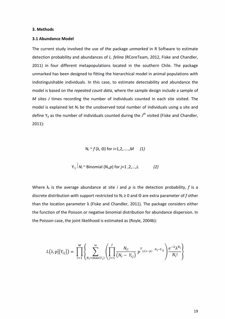
3. Methods
3.1 Abundance Model
The current study involved the use of the package unmarked in R Software to estimate
detection probability and abundances of L. felina (RCoreTeam, 2012, Fiske and Chandler,
2011) in four different metapopulations located in the southern Chile. The package
unmarked has been designed to fitting the hierarchical model in animal populations with
indistinguishable individuals. In this case, to estimate detectability and abundance the
model is based on the repeated count data, where the sample design include a sample of
M sites J times recording the number of individuals counted in each site visited. The
model is explained let Ni be the unobserved total number of individuals using a site and
define Yij as the number of individuals counted during the Jth visited (Fiske and Chandler,
2011):
Ni ~ f (λ, Θ) for i=1,2,…..,M (1)
Yi j Ni ~ Binomial (Ni,p) for j=1 ,2,…,Ji (2)
Where λi is the average abundance at site i and p is the detection probability, f is a
discrete distribution with support restricted to Ni ≥ 0 and Θ are extra parameter of f other
than the location parameter λ (Fiske and Chandler, 2011). The package considers either
the function of the Poisson or negative binomial distribution for abundance dispersion. In
the Poisson case, the joint likelihood is estimated as (Royle, 2004b):
��λ, p����� �� � �� �!�� ������������ ��� ��!"# $%
&�"'()����*+,λ&��! -.
"#
20
The model includes the use of covariate as state or detection levels being the abundance
estimated as follows:
Log(λi)=xiTß, (4)
Where xi is a vector of site-level covariate and ß is a vector of their corresponding effect
parameter (Fiske and Chandler, 2011).
The model for detection probability is:
Logit(pij)=vijTα, (5)
Where vij is a vector of observation-level covariates and α is a vector of their
corresponding effect parameter (Fiske and Chandler, 2011).
3.2 Study area Description
This methodology was applied to two set of data, both from areas situated in the
southern Chile. The first study area is located on the Valdivian coastline (39ºS – 73ºW).
The area is characterized by a rocky shore exposed to the wave, formed by rocky cliff,
rocky and sandy beach, where the coastline have a width about 10 m average. The
coastline shows a westerly general aspect with a high energy as results of the wave
exposure making difficult the access by sea. The area show a typical biodiversity of
temperate intertidal zones mainly influences by the Humboldt Current and human use
(Jara and Moreno, 1984, Moreno et al., 2001). Four sites were sampled in the study area
during a period of 12 months. The samplings were carried out between July 1999 and
June 2000.

21
Figure 1. Study area first dataset
The second study area encompasses three large and diverse geographic zones located
south of the first study area, which, since a Metapopulation approach, could be
considered three different metapopulations, because the interchange of species between
these areas could be low, due to the spatial distance between them and the weather
condition during the year. The first zone is Chiloé Island (41º46’ – 46º59’ S to 72º30’ –
75º26’) in the Chiloé Archipelago extending 180 km from north to south. The island’s
northern and southern shore is separated from the continent by the Ancud and
Corcovado Gulf (Figure 2). The second zone is Continental Chiloé or the Province of
Palena. In general terms, this sector is where the Central Valley disappears due to erosion
and flooding produced in the Quaternary Period, created the Chiloé inland sea. As a
result, geographically speaking, the area of Palena is considered part of the Andes Range,
the glacial activity in zones adjacent to the Andes Range also created the fjords and
channels that exist today (Subiabre and Rojas, 1994). The third study zone is located
south of the Chiloe Island; the zone is dominated by islands, channels and fjords, and
corresponds to the submerged costal range, formed and shaped as a result of tectonics

22
and glacial processes. The zone includes areas The Guaitecas Archipelago, where the
surveys were carried out; Chonos Archipelago and the area of Taitao Peninsula furthest
south (Figure 2). These areas are located within an oceanic ecological region of
Mediterranean influence, with annual precipitation measuring 2,000 – 2,500 mm, an
average relative humidity of 84%, a historic annual average temperature of 10.5 ºC, and
minimum and maximum temperatures averaging 6.9º C and 14.2º C respectively
(Subiabre and Rojas, 1994, Villalobos et al., 2003).
Figure 2. Study Area second data analysed.
3.3 Sampling Data
3.3.1 First data set
In this case the data of the survey was collected and published in Medina-Vogel et al.
(2006). Four sites along of the coastline were surveyed through of three watcher situated
every ±300 m in average (Fig. 1). The distance between sites was about 1.4 – 1.6 km each
other. Every point count site was surveyed scanning the area with 10x50 binoculars for a
period of two minutes every eight minutes in the area covered by each watcher, which

23
was identified by natural marks. The period of surveys was divided in two periods
(morning-afternoon) during one year in a maximum of 12 hours and a minimum of 8
hours per site surveyed and where every site was visited once a month. The data set used
in this model was the results of surveys developed by one watcher. Despite the limited
number of sites, the long periods of watching for each visited allow using a robust
modelling of detectability (large K could be used). However the lack of site replication
prevents any useful inference of abundance.
3.3.2 Second data set
This data set was collected through of fieldwork campaigns carried out by a Chilean NGO
Conservacion Marina by means of the marine otter conservation initiative. The first
campaign was carried out in March 2006 and March 2007, the second campaign was in
October 2008 and February 2009 and the last campaign was in March 2012. The survey
methodology was a modification of the method used by Medina-Vogel et al. (2006). Each
census was carried out by three observers located in vantage points along the ±1 km
transect. Observers recorded the presence of otters and their activities during four
continuous hours helping by two-ways radios, to avoid double counted. For each scan,
observers recorded the otter position in the portion of transect under observation on a
reference map. All the observations were made with the aid of 10x50 power view
binoculars.
3.4 Use of the Unmarked and Multi-model inference package in R
The package use the S4 class system called unmarkedFrame, which compile the
information of the sampling design, which allow organize the data and use the functions
programming into it (Chambers, 2008). The unmarkedFrame is organized in three
components called slots, one slot contains the observation matrix y and a data.frame for
site-level covariate and another for observation-level covariate (Fiske and Chandler,
2011). In both data set was used the UnmarkedFramePCount function, which is entered
in the package as pcount. Later, were entered the functions fitlist and modelsel, which
organize and selected the models fitted. Finally the function model.avg of the package
MuMIn (Multi-model inference) was used to obtain the average values of the models and
the value of importance from the covariates in the model (Barton, 2012)
24
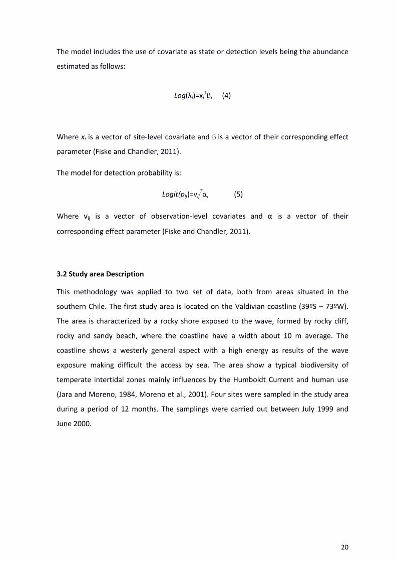
3.4.1 Observation Matrix y.
The first data set was fitted in a matrix of M=27 rows on J=12 visits (columns). The rows
correspond to the sites visited during the year of sampling and column to the intervals of
hour in which was divided the period of survey. In each visit was recorded the number
maximum of otter recorded simultaneously (Table 2).
Table 2. First data set matrix, the rows correspond to the site visited and the columns to the
visits divided per hour interval. The command only shows the data until the row 5. Matrix cells
contain numbers of otters counted in each hour, and times are hourly from x:0 – y:00 for t1
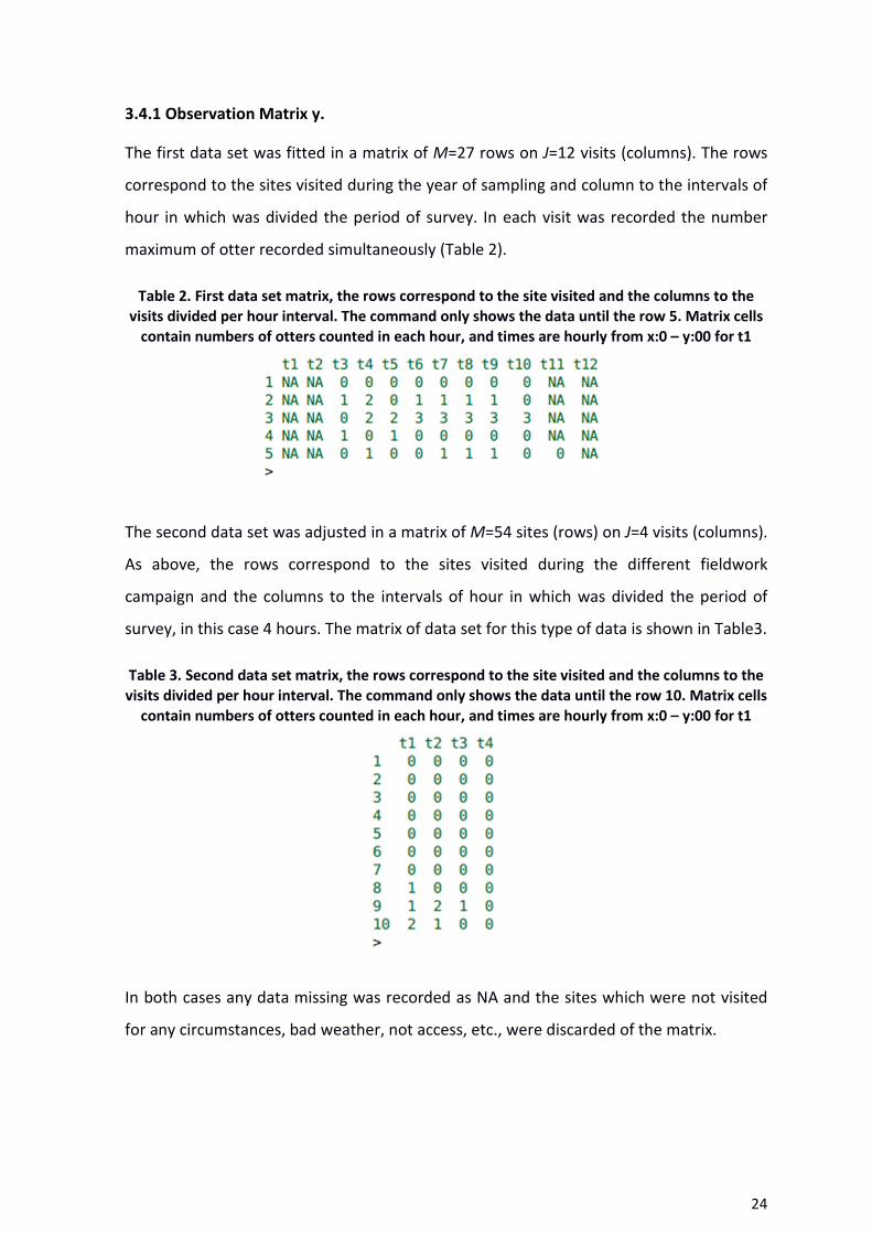
The second data set was adjusted in a matrix of M=54 sites (rows) on J=4 visits (columns).
As above, the rows correspond to the sites visited during the different fieldwork
campaign and the columns to the intervals of hour in which was divided the period of
survey, in this case 4 hours. The matrix of data set for this type of data is shown in Table3.
Table 3. Second data set matrix, the rows correspond to the site visited and the columns to the
visits divided per hour interval. The command only shows the data until the row 10. Matrix cells
contain numbers of otters counted in each hour, and times are hourly from x:0 – y:00 for t1
In both cases any data missing was recorded as NA and the sites which were not visited
for any circumstances, bad weather, not access, etc., were discarded of the matrix.
25
3.4.2 Covariates
The repeated count data model includes the use of site-level covariates and observation-
level covariate to modelling the probability of detection (log λ) and abundance (logit ß).
One important aspect to be considered in the arrangement of the covariate is that the
fitting with the observation matrix, this means, that the numbers of rows (sites) have to
match with every row from the covariate considering in the model. The covariates used in
both data sets are included in the appendices E and F.
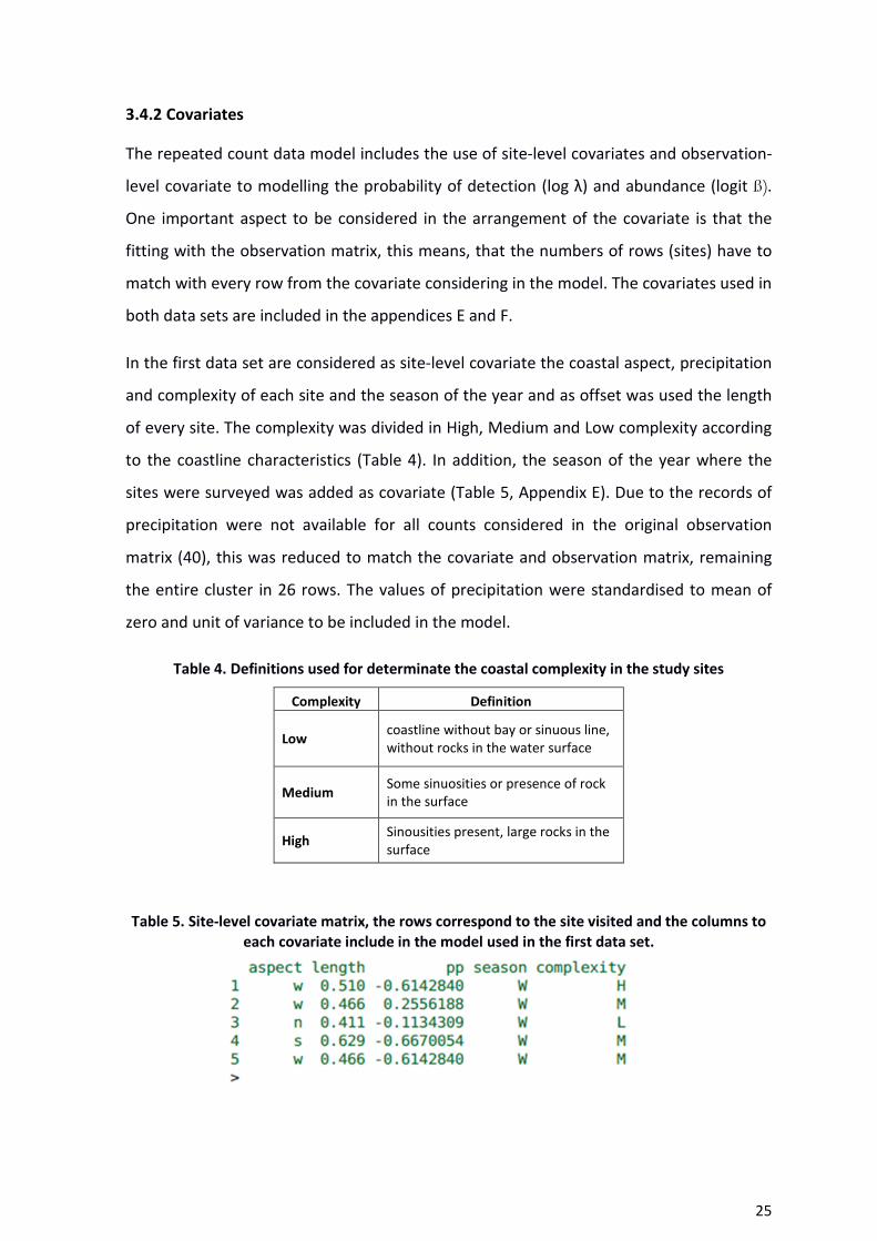
In the first data set are considered as site-level covariate the coastal aspect, precipitation
and complexity of each site and the season of the year and as offset was used the length
of every site. The complexity was divided in High, Medium and Low complexity according
to the coastline characteristics (Table 4). In addition, the season of the year where the
sites were surveyed was added as covariate (Table 5, Appendix E). Due to the records of
precipitation were not available for all counts considered in the original observation
matrix (40), this was reduced to match the covariate and observation matrix, remaining
the entire cluster in 26 rows. The values of precipitation were standardised to mean of
zero and unit of variance to be included in the model.
Table 4. Definitions used for determinate the coastal complexity in the study sites
Complexity Definition
Low coastline without bay or sinuous line, without rocks in the water surface
Medium Some sinuosities or presence of rock in the surface
High Sinousities present, large rocks in the surface
Table 5. Site-level covariate matrix, the rows correspond to the site visited and the columns to
each covariate include in the model used in the first data set.

26
In relation to the observation-level covariate in this data set were considered two types
of variables. Firstly was considered the time of day which was carried out the survey
morning (m) or afternoon (a) (Table 6).
Table 6. Time of day arrangement used as observation-level and divided in Morning or
Afternoon periods in the first data set.
The second observation-level covariate was the tide level present during the day, either
high tide (HT) or low tide (LT) (Table 7).
Table 7. Tide level arrangement used as observation-level covariate
For the second data set were considered as site-level covariate the weather conditions
during the survey in each site (Cloudy, Rainy, and Sunny), the complexity of the coastline
(High, Medium, and Low), the aspect of the site in the area and the length of every site
was used as a covariate in the model (Table 8).
Table 8. Site-level covariate matrix, the rows correspond to the site visited and the columns to
each covariate include in the model used in the second data set.
Finally, as observation-level covariate the time of the day, which was carried out the
survey was added in the model (morning or afternoon) (Table 9). Tide was not included as

27
a covariate due to the complexity to estimate it for each site along of the area, due to the
point of reference to estimate the tide is located away of the site southern and the tide
effect could be sub estimated.
Table 9. Observation-level matrix for the second data set.

28
4. Results
4.1 First Data Set
As shown from the AIC values assigned to the models in Table 10, of the 32 models run in
R (see Appendices A and B), three models are relevant to the data. According to the
values of AICΔ the models p(D+S), p(D+T+S+C), and p(D+S+P) best fit the data following
the rules of AICΔ< 2 asserted by Burnham and Anderson (2002). The differences in AICw
between the first and the other models are weak because the evidence ratio is low, just
1.8 between the first and second models; and 2.02 between the first and third.
Table 10. Values of AIC, AICΔ and AIC weights for the five best models estimated from the first
data set. In all models, abundance (λ) was modelled with no covariates but the log of length of
coast covered as an offset. Covariates are coded as D: time of day, S: season. T: tide, C:
complexity, P: precipitation
Model1
AIC AICΔ AICw
p(D+S) 493.54* 0 0.2288
p(D+T+S+C) 494.74* 1.2 0.1257
p(D+S+P) 494.95* 1.41 0.1131
p(T+S) 495.91 2.37 0.0701
P(D+T+S+C+P) 496.23 2.69 0.0597
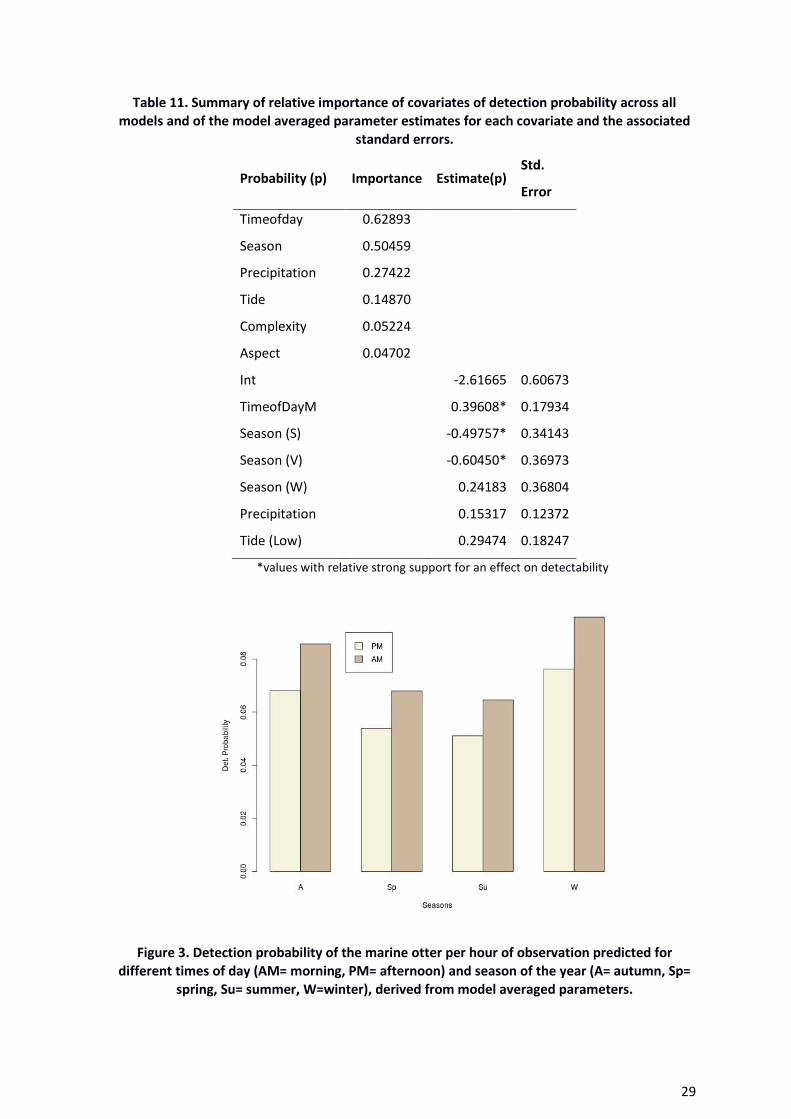
The detection probability in this data set is dominated by two covariates, the Time of Day
and Season covariates, with relatively strong support for effects of these covariates.
There is some support for effects of precipitation, tide and complexity, although much
weaker (Table 11). The average estimation shows close values between the covariates,
with the most important being Time of Day (Morning), Season spring (S) and summer (V).
Real detection probabilities were derived by back-transforming model averaged
parameter estimates split by time of day and season (Figure 3). This showed that, the
most likely time to detect a marine otter was during the morning and principally during
winter and autumn, spring was slightly less likely and the lowest probability was for both
intervals during the summer (Figure 3).
29
Table 11. Summary of relative importance of covariates of detection probability across all
models and of the model averaged parameter estimates for each covariate and the associated
standard errors.
Probability (p) Importance Estimate(p) Std.
Error
Timeofday 0.62893
Season 0.50459
Precipitation 0.27422
Tide 0.14870
Complexity 0.05224
Aspect 0.04702
Int
-2.61665 0.60673
TimeofDayM
0.39608* 0.17934
Season (S)
-0.49757* 0.34143
Season (V)
-0.60450* 0.36973
Season (W)
0.24183 0.36804
Precipitation
0.15317 0.12372
Tide (Low) 0.29474 0.18247
*values with relative strong support for an effect on detectability
Figure 3. Detection probability of the marine otter per hour of observation predicted for
different times of day (AM= morning, PM= afternoon) and season of the year (A= autumn, Sp=
spring, Su= summer, W=winter), derived from model averaged parameters.

30
4.2. Second Data Set
A total of 61 models were run within the data set (Appendix C and D), a summary with
the most important models results are shown in Table 12. According to the values of AICΔ,
the model p(W+A+C+D)(C) best fit the data according to the rules of AICΔ< 2. The AIC
weights assigned to the models confirm the robustness of p(W+A+C+D)(C) in relation to
the other values, because the evidence ratio is 5.5 between the first and second models
and 9.3 times between the first and third models (Table 12). In addition, given the results
of AICw, the second model provides a similar description of the data, but is dismissed by
virtue of its AICΔ value. The Model p(W+A+C+D)(C) grouped all site-level covariate to
probability of detection and also considered the length as an offset, as well as complexity
for the abundance estimation (Table 12).
Table 12. Values of AIC, AICΔ and AIC weights for the five best models estimated from the first
data set. In the first model, abundance (λ) was modelled with Complexity and Aspect as
covariates and the log of length of coast covered as an offset. Covariates are coded as D: time
of day, W: weather. A: aspect, C: complexity.
Model1 AIC AICΔ AICw
p(W+A+C+D)(C) 283.87 0 0.67
p(A+T+C) 287.29 3.42 0.12
p(W+A+C+D)(C+A) 288.25 4.38 0.072
p(T+C)(C) 290.75 6.89 0.02
p(A+T+C)(C+A) 290.91 7.04 0.019
In relation to detection probability the site-level covariate with the most influence in this
model was time of day, followed by the weather and complexity covariate, which had a
lower degree of influence on the model (Table 13).
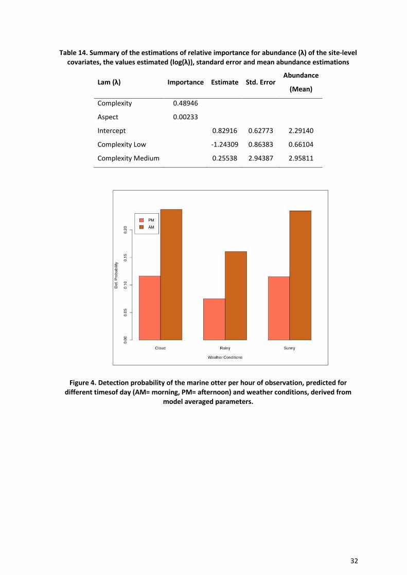
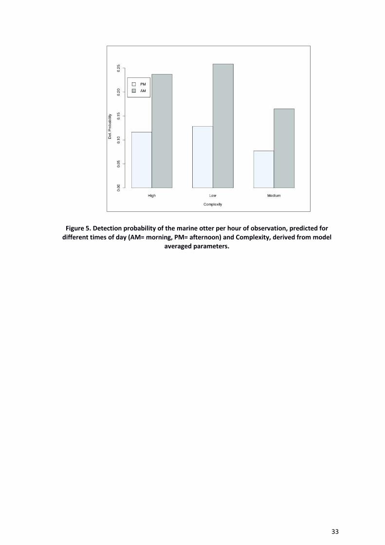
The model averaged parameter estimates show that detectability is higher in the morning
than the afternoon (Table 13, Figure 4 and 5); while detectability is reduced during rainy
weather relative to either cloudy or sunny conditions (Figure 4). There was also some
evidence of reduced detectability in medium complexity coastline relative to either high
or low complexity, although this effect was weak (Table 13, Figure 5).

31
Table 14 shows the importance value for the abundance estimation of L. felina. To obtain
the real values of abundance, the values of the model averaged parameter were back-
transformed split by complexity (the most relevant covariate in the model), complexity
high and complexity low were the most prominent. The estimation of abundance is
around 2.29 ind/km, with a lowest value for Complexity Low of 0.66 ind/km and higher
value of 2.95 ind/km for Complexity Medium.
Table 13. Summary of the estimations of relative importance for detection probability of the
site-level and observation-level covariates and the values estimated (p) in each covariate with
the associated standard error.
Probability (p) Importance Estimate Std.
Error
Timeofday 0.88596
Weather 0.35777
Complexity 0.33120
Aspect 0.02185
Int
-2.02687 0.81918
TimeofDayM
0.96911 0.35795
Weather Rainny
-1.35354 0.72884
Weather Sunny
-0.0387 0.41661
Complexity Low
0.34686 1.64888
Complexity Medium
-1.3678 3.57412
Aspect (N)
-0.3146 1.02662
Aspect (NE)
1.55351 1.13072
Aspect (NW)
-0.52 1.23607
Aspect (S)
1.00154 1.17479
Aspect (SE)
0.69791 1.22456
Aspect (SW)
0.96303 1.14292
Aspect (W)
-0.8344 0.98378
Complexity Low
-1.24309 0.86383
Complexity Medium 0.25538 2.94387
32
Table 14. Summary of the estimations of relative importance for abundance (λ) of the site-level
covariates, the values estimated (log(λ)), standard error and mean abundance estimations
Lam (λ) Importance Estimate Std. Error Abundance
(Mean)
Complexity 0.48946
Aspect 0.00233
Intercept
0.82916 0.62773 2.29140
Complexity Low
-1.24309 0.86383 0.66104
Complexity Medium 0.25538 2.94387 2.95811
Figure 4. Detection probability of the marine otter per hour of observation, predicted for
different timesof day (AM= morning, PM= afternoon) and weather conditions, derived from
model averaged parameters.
33
Figure 5. Detection probability of the marine otter per hour of observation, predicted for
different times of day (AM= morning, PM= afternoon) and Complexity, derived from model
averaged parameters.

34
5. Discussion
Population studies on the marine otter are scarce, and methodologies that allow the
estimation and monitoring of otter populations are not developed. This study is the first
attempt to propose a methodology that allows a reliable estimation of population density
of the marine otter, and from there to estimate a population in at a metapopulation
level. The data analysed according to N-mixtures models based on binomial and Poisson
distribution show suitable rec sults that are well adjusted to the model proposed by Royle
(2004b).
5.1 Performance of covariates and estimations
The results of the first and second data set showed three different models that fitted the
data reasonably well and a single model has strong support (Table 10 and 12). These
results are relevant, considering the first data set, because they explain that the models
show uncertainty, which may affect detectability. This might be because the key
covariates are missing, while those available are too crude to capture the underlying
process well. In particular, the number of sites in this analysis was extremely limited,
which undoubtedly presents difficulties in finding good sites-level covariates. Secondly
place, the presence of a single model shows data and covariates that are more reliable at
estimating detection probability and abundance, considering the data of the second data
set.
In terms of probability of detection, despite a degree of uncertainty in the first data set in
model selection, there was reasonably strong support for time of day and season as
predictors of detectability. Importance of these covariates is confirmed with the values of
the second data set, where two of the most important covariates are matched, the time
of day, and complexity of coastline, more the third covariate weather. This is a relevant
element mentioned by Royle (2004b), who proposed that covariates have to explain the
spatial variation of the metapopulation unit along the sites where the abundance is
estimated.

35
In relation to time of day, the estimations show higher probability of detection in the
morning for both data sets mainly in winter and autumn in the first data set and high and
low complexity in the second. This could be associated with the behaviour of the otters,
because in general, it is assumed that otters have crepuscular or nocturnal activity (Ruiz-
Olmo et al., 2001). Coincidently in the same area higher activity in the morning was
reported, but only in the summer season (Medina-Vogel et al., 2006). Although later, a
study with radio-telemetry on the species carried out in central-Chile suggested that
there is no preference for activity in relation to time of day (Ruiz-Olmo et al., 2001,
Medina-Vogel et al., 2006, Medina-Vogel et al., 2007). However, further studies to
analyse this issue could be performed.
There was no explanation in the results obtained for probability of detection derivate
from the complexity covariate, although is possible suppose that the habitat selection of
the marine otter could play a particular role in it (Ebensperger and Castilla, 1992,
Ebensperger and Botto-Mahan, 1997, Medina-Vogel et al., 2006, Kruuk, 2006). These
results could indicate that posterior studies including new covariates (i.e. new values of
complexity or new ways to measure it) have to be included. However, it is possible to
suggest that complexity, weather and time of day covariates might be useful in the
implementation of monitoring planning in order to maximize effort and reduce fieldwork
costs.
In relation to other covariates included in both models, although it is conceivable for the
first data set that the precipitation covariate could play a relevant role in the probability
of detection due to affecting the vision of the watcher; results assigned it a low
importance. This may be because the fieldworks was planned during days of low rain
probability and were cancelled during bad weather conditions. Tide was also assigned
lower importance in the models, which might produce the low influence between the
levels of high and low tide in the area. Finally, it could be expected that the probability of
detection was higher in summer or spring, due to good weather conditions expected;
however according to results, winter and autumn show the best probability (Figure 3).
This could be produced by the absence of precipitation in that period, which is
corroborated with the low importance of that covariate. To obtain a better

36
understanding of these results add a covariate (observation-level) that explains with
more detail the change in weather or environmental condition in the site could be used.
Unlike the first data set, weather during surveys was more variable, and rainy weather
was found to affect detection probability negatively, likely because the surveys were not
cancelled during the fieldwork due to the campaigns having a short time to be carried
out. This is relevant for monitoring and posterior studies to help confirm the avoidance of
surveys in rainy periods. Finally, in this data set the values estimated for aspect, show a
low value of importance, this is contradictory because aspect appears to be relevant for
this data set , with the three most important model and have no a clear explanation
(Table 12 and 13).
In relation to abundance include here only for the second data set, this was higher on
more complex coastlines, with medium and high complexity sites having numbers per km
of coastline around 3-4 times higher than on simple coastlines. This may be because, as a
first approximation, the levels complexity could be linked to some type of habitat and/or
prey availability for marine otter (Ebensperger and BottoMahan, 1997, Ebensperger and
Castilla, 1992, Ostfeld et al., 1989). Preliminarily, the importance of complexity could
have a direct influence on conservation measures for otters because this could be a
pattern identifying the estimation of spatial occurrence/distribution for this specie.
However, issues that need further attention, are the relationship between complexity
and type of habitat, size of fragments and foraging behaviour of the marine otter (Villegas
et al., 2007, Medina-Vogel et al., 2008). As was explained above, previous studies are not
entirely comparable with this study because the methodologies of estimation are
different. However it is possible to mention that abundances in this study are similar to
those reported in previous studies, which give a credibility framework to the values
estimated with this approach. Using this perspective, there are similarities in estimation
between both northern and southern Chile, particularly for the values estimated by Rozzi
and Torres-Mura (1990) who carried out their study in similar areas (Table 1).
37
5.2 Method Performance
The use of the repeated counts methods to estimate abundance from small population
size, low probability of detection and unmarked populations using N-mixture distribution
models, seems to be reliable due to the estimates obtained, which makes it advisable to
use with this species if the assumptions are meet. One of the elements that have to be
considered to perform this approach in estimating abundance successfully is to avoid
violation of the assumptions. A key assumption of the repeated count model is
population closure during surveys. This means that while the individuals are surveyed the
interchange of individuals between one area and another could be produced by
temporary or permanent migration (through of births and deaths) (Royle, 2004a, Royle,
2004b, Chandler et al., 2011). There is a probability that this assumption was violated in
the first data set due to the distance between sites being less that the home-range
estimated for otters (Medina-Vogel et al., 2007), however the census were carried out on
different days and it assumes that the overlap is remains constant, i.e. “the site super-
population” (Dail and Madsen, 2011), might suggest that this assumption is upheld.
One important element in application of effective conservation measures on the marine
otter is to obtained regular information species trend. One way, is through the design of
population monitoring, which would violate the closed population assumption due to
temporal emigration between the monitored sites (Chandler et al., 2011). In this sense,
the comparison of estimated abundance of a data set from open populations is not
applicable and other distributions and methods are necessary (Dail and Madsen, 2011,
Chandler et al., 2011). One solution has been the development of metapopulation
dynamics designed based on the generalization of the N-mixture model obtained by
Royle (2004a), which have been included in the unmarked package (Fiske and Chandler
2001). This modification allows estimates and compares abundances in open populations
between the same sample points, which might be easily included in a monitoring
program that considers fixed point samples and is recommended to use together with
this model to estimate abundance of the marine otter.
Some applications of this methodology in fieldwork consider the design of the survey
with one watcher per site, this way the double counted and/or the overestimations of the

38
survey length site is avoided. In relation to length of site cover for every watcher, at more
precise estimation of the site distance is required, as the literature has mentioned that
assumptions for this type of covariate are difficult to meet (Efford and Dawson, 2009).
Finally, some issues for further studies are to understand the minimum number of survey
sites and repeats to obtain reliable population estimation. To determine the importance
of the optimal length of each survey site and the assessment of covariates that fit best
the data collected in order to explain the probability of detection and abundance of the
otter. This is because many studies are based on avian abundance estimation. Further
studies could compare the performance and reliability of the N-mixture model with
estimations of abundance based on genetic analysis, such has been estimated for Lutra
lutra (Hung et al., 2004) and recently for Lontra longicaudis (Trinca 2011) , combining
these techniques with molecular techniques and the Capture-Mark-Recapture approach
may be beneficial (Petit and Valiere, 2006, Coster et al., 2011)

39
6. References
ALVAREZ, R. & MEDINA-VOGEL, G. 2008. Lontra felina. IUCN Red List of Threatened Species
[Online]. ASTUA, D., ASFORA, P., ALESSIO, F. & LANGGUTH, A. 2010. On the occurrence of the Neotropical
Otter (Lontra longicaudis) (Mammalia, Mustelidae) in Northeastern Brazil Mammalia, 74, 213-217.
BART, J., DROEGE, S., GEISSLER, P., PETERJOHN, B. & RALPH, C. J. 2004. Density estimation in wildlife surveys. Wildlife Society Bulletin, 32, 1242.
BARTON, K. 2012. MuMIn: Multimodel Inference. R package version 1.7.11. In: HTTP://CRAN.R-PROJECT.ORG/PACKAGE=MUMIN (ed.).
BURNHAM, K. P. & ANDERSON, D. R. 2002. Model Selection and Multimodel Inference Springer-Verlag New York Inc.
CAAP 2008. Capitulo 4. Diversidad Biólogica. In: CAAP (ed.) Informe País Estado del Medio
Ambiente en Chile 2008.
CASARIEGO-MADORELL, A., MARIA LIST, R. & CEBALLOS, G. 2008. Population size and the diet of the river otter (lontra longicaudis annectens) on the Oaxaca coast, Mexico. Acta zoológica
mexicana, 24, 179-199. CASTILLA, J. C. 1982. Nuevas observaciones sobre conducta, ecología y densidad de Lutra felina
(Molita 1782)(Carnivora: Mustelidae) en la zona central y centro-norte de Chile. . Archivos de Biología y Medicina Experimentales, 13.
CASTILLA, J. C. & BAHAMONDES, I. 1979. Behavioral and Ecological Observations in Lutra-Felina (Molina) 1782 (Carnivora, Mustelidae) in Central and North-Central Zones of Chile. Archivos de Biologia y Medicina Experimentales, 12, 119-131.
CHAMBERS, J. M. 2008. Software for Data Analysis: Programming with R Springer. CHANDLER, R. B., ROYLE, J. A. & KING, D. I. 2011. Inference about density and temporary
emigration in unmarked populations. Ecology, 92, 1429-1435. CHEHEBAR, C. E. Y. 1985. A Survey of the Southern River Otter Lutra p r o v o c a x Thomas in
Nahuel Huapi National Park , Argentina. Biological Conservation, 32, 299-307. COSTER, S. S., KOVACH, A. I., PEKINS, P. J., COOPER, A. B. & TIMMINS, A. 2011. Genetic Mark-
Recapture Population Estimation in Black Bears and Issues of Scale. Journal of Wildlife
Management, 75, 1128-1136. DAIL, D. & MADSEN, L. 2011. Models for Estimating Abundance from Repeated Counts of an Open
Metapopulation. Biometrics, 67, 577. DODD, C. K. & DORAZIO, R. M. 2004. Using counts to simultaneously estimate abundance and
detection probabilities in a salamander community Herpetologica, 60, 468-478. DORAZIO, R. M. 2007. On the choice of statistical models for estimating occurrence and extinction
from animal surveys. Ecology, 88, 2773. EBENSPERGER, L. A. & BOTTO-MAHAN, C. 1997. Use of habitat, size of prey, and food-niche
relationships of two sympatric others in southernmost Chile Journal of mammalogy, 78, 222-227.
EBENSPERGER, L. A. & BOTTOMAHAN, C. 1997. Use of habitat, size of prey, and food-niche relationships of two sympatric otters in southernmost Chile. Journal of mammalogy, 78, 222-227.
EBENSPERGER, L. A. & CASTILLA, J. C. 1991. Behavior and population density of Lutra felina at Isla Pan de Azucar (III Region), Chile. Medio Ambiente, 11, 79-83.
EBENSPERGER, L. A. & CASTILLA, J. C. 1992. Habitat Selection in Land by the Marine Otter, Lutra-Felina, at Pan-De-Azucar-Island, Chile. Revista Chilena De Historia Natural, 65, 429-434.
EFFORD, M. G. & DAWSON, D. K. 2009. Effect of Distance-Related Heterogeneity on Population Size Estimates from Point Counts. Auk, 126, 100.
40
FARNSWORTH, G. L., POLLOCK, K. H., NICHOLS, J. D., SIMONS, T. R., HINES, J. E. & SAUER, J. R. 2002. A removal model for estimating detection probabilities from point-count surveys. Auk, 119, 414.
FISKE, I. J. & CHANDLER, R. B. 2011. unmarked : An R Package for Fitting Hierarchical Models of Wildlife Occurrence and Abundance. Journal of Statistical Software, 43, 23.
GUTER, A., DOLEV, A., SALTZ, D. & KRONFELD-SCHORA, N. 2008. Using videotaping to validate the use of spraints as an index of Eurasian otter (Lutra lutra) activity. Ecological Indicators, 8, 462-465.
HUNG, C.-M., LI, S.-H. & LEE, L.-L. 2004. Faecal DNA typing to determine the abundance and spatial organisation of otters (Lutra lutra) along two stream systems in Kinmen. Animal
Conservation, 7, 301-311. JARA, H. F. & MORENO, C. A. 1984. Herbivory and Structure in a Midlittoral Rocky Community - a
Case in Southern Chile. Ecology, 65. KRUUK, H. 2006. Otters : ecology, behaviour, and conservation, Oxford University Press. KRUUK, H. & CONROY, J. W. H. 1987. Surveying otter Lutra lutra populations: A discussion of
problems with spraints. Biological Conservation, 41, 179-183. LARIVIERE, S. 1998. Lontra felina. Mammalian Species, 0, 1. LARIVIERE, S. 1999. Lontra provocax. Mammalian Species, 1-4. LIMA, D. D. S., MARMONTEL, M. & BERNARD, E. 2012. Site and refuge use by giant river otters
(Pteronura brasiliensis) in the Western Brazilian Amazonia. Journal of Natural History, 46, 729-739.
MACKENZIE, D. I., NICHOLS, J. D., HINES, J. E., KNUTSON, M. G. & FRANKLIN, A. B. 2003. Estimating site occupancy, colonization, and local extinction when a species is detected imperfectly. Ecology, 84, 2200.
MACKENZIE, D. I., NICHOLS, J. D., LACHMAN, G. B., DROEGE, S., ROYLE, J. A. & LANGTIMM, C. A. 2002. Estimating site occupancy rates when detection probabilities are less than one. Ecology, 83, 2248.
MACKENZIE, D. I., NICHOLS, J. D., ROYLE, J. A., POLLOCK, K. H., BAILEY, L. L. & HINES, J. E. Y. 2006. Occupancy estimation and modeling, Academic Press Inc.
MACKENZIE, D. I. & NICHOLS, J. D. Y. 2004. Occupancy as a surrogate for abundance estimation. Animal Biodiversity and Conservation, 461-467.
MACKENZIE, D. I. & ROYLE, J. A. 2005. Designing Occupancy Studies: General Advice and Allocating Survey Effort. Journal of Applied Ecology, 42, 1105.
MASON, C. F. & MACDONALD, S. M. 1987. The use of Spraints for Surveying Otter Lutra-Lutra Populations - an Evaluation Biological Conservation, 41, 167-177.
MEDINA-VOGEL, G., BARTHELD, J. L., PACHECO, R. A. & RODRIGUEZ, C. D. 2006. Population assessment and habitat use by marine otter Lontra felina in southern Chile. Wildlife
Biology, 12, 191-199. MEDINA-VOGEL, G., BOHER, F., FLORES, G., SANTIBANEZ, A. & SOTO-AZAT, C. 2007. Spacing
behavior of marine otters (Lontra felina) in relation to land refuges and fishery waste in central Chile. Journal of mammalogy, 88, 487-494.
MEDINA-VOGEL, G., MERINO, L. O., ALARCON, R. M. & VIANNA, J. D. A. 2008. Coastal-marine discontinuities, critical patch size and isolation: implications for marine otter conservation. Animal Conservation, 11, 57-64.
MORENO, C., JARAMILLO, E. & LEPEZ, I. 2001. Estudio de áreas potenciales de reservas marinas y parques marinos entre la VIII y la X regiones. Informe final Proyecto FIP 99-29.
Universidad Austral de Chile, Universidad de Concepción., 1, 90. NICHOLS, J. D., HINES, J. E., SAUER, J. R., FALLON, F. W., FALLON, J. E. & HEGLUND, P. J. 2000. A
double-observer approach for estimating detection probability and abundance from point counts. Auk, 117, 393-408.

41
OSTFELD, R. S., EBENSPERGER, L., KLOSTERMAN, L. L. & CASTILLA, J. C. 1989. Foraging, Activity Budget, and Social-Behavior of the South-American Marine Otter Lutra-Felina (Molina 1782). National Geographic Research, 5, 422-438.
PETIT, E. & VALIERE, N. 2006. Estimating population size with noninvasive capture-mark-recapture data. Conservation Biology, 20, 1062-1073.
PICKLES, R. S. A., GROOMBRIDGE, J. J., ZAMBRANA ROJAS, V. D., VAN DAMME, P., GOTTELLI, D., KUNDU, S., BODMER, R., ARIANI, C. V., IYENGAR, A. & JORDAN, W. C. 2011. Evolutionary history and identification of conservation units in the giant otter, Pteronura brasiliensis Molecular phylogenetics and evolution, 61, 616-327.
QUADROS, J., LEITE, E. & MONTEIRO FILHO, A. 2002. Sprainting sites of the neotropical otter, Lontra longicaudis, in an Atlantic Forest area of southern Brazil. Mastozoología
neotropical, 9, 39-46. RCORETEAM 2012. R: A Language and Environment for Statistical Computing. In: R FOUNDATION
FOR STATISTICAL COMPUTING, V., AUSTRIA. (ed.) R Foundation for Statistical Computing,
Vienna, Austria.
ROYLE, J. A. 2004a. Generalized estimators of avian abundance from count survey data. Animal
Biodiversity and Conservation, 27, 375. ROYLE, J. A. 2004b. N-mixture models for estimating population size from spatially replicated
counts. Biometrics, 60, 108. ROYLE, J. A. & DORAZIO, R. M. 2008. Hierarchical Modeling and Inference in Ecology, Academic
Press; 1 edition ROYLE, J. A. & NICHOLS, J. D. 2003. Estimating abundance from repeated presence-absence data
or point counts. Ecology, 84, 777. ROYLE, J. A., NICHOLS, J. D. & KÉRY, M. 2005. Modelling occurrence and abundance of species
when detection is imperfect. Oikos, 110, 353. ROZZI, R. & TORRES-MURA, J. 1990. The South American Sea Otter Lutra-Felina Observed South of
Chiloe Island South Pacific Ocean Background for its Conservation. Medio Ambiente, 11, 24-28.
RUIZ-OLMO, J., SAAVEDRA, D. & JIMENEZ, J. 2001. Testing the surveys and visual and track censuses of Eurasian otters (Lutra lutra) Y1 - 2001. Journal of zoology, 253, 359-369.
SEPULVEDA, M. A., BARTHELD, J. L., MEYNARD, C., BENAVIDES, M., ASTORGA, C., PARRA, D. & MEDINA-VOGEL, G. 2009. Landscape features and crustacean prey as predictors of the Southern river otter distribution in Chile. Animal Conservation, 12, 522-530.
SEPULVEDA, M. A., BARTHELD, J. L., MONSALVE, R., GOMEZ, V. & MEDINA-VOGEL, G. 2007. Habitat use and spatial behaviour of the endangered Southern river otter (Lontra provocax) in riparian habitats of Chile: Conservation implications. Biological Conservation, 140, 329-338.
SIELFELD, W. 1992. Abundancias relativas de Lutra felina(Molina 1782) y L. provocax (Thomas 1908) en el litoral de Chile austral. Invest. Cient. Y Tec., Serie Ciencias del Mar 2, 3-11.
SIELFELD, W. & CASTILLA, C. 1999. ESTADO DE CONSERVACIÓN Y CONOCIMIENTO DE LAS NUTRIAS EN CHILE SCIENTIFIC La distribución pasada y actual de Lontra provocax y su declinación poblacional en Chile centro sur ( 36 ° 46 ° Lat . S ) han sido analizados y discutidas por MEDINA ( 1991 y 1996 ). Estud. Oceanol., 18, 69-79.
SUBIABRE, A. & ROJAS, C. 1994. Geografía Física de la Región de Los Lagos. TRINCA, C. S. 2012. Historia evolutiva e ecologia molecular da lontra netropical (Lontra
longicaudis)(Carnivora:Mustelidae). Doutorado, Universidade Federal do Rio Grande do Sul.
VALQUI, J. 2012. The marine otter Lontra felina (Molina, 1782): A review of its present status and implications for future conservation. Mammalian Biology, 77, 75.
VAZ FERREIRA, R. 1976. Situación Poblacional y conservación de los mamíferos marinos en Latinoamerica. Acta Zoologica Liloana, 34, 91-101.

42
VILLALOBOS, L., PARRA, O., GRANDJEAN, M., JAQUE, E., WOELFL, S. & CAMPOS, H. Y. 2003. A study of the river basins and limnology of five humic lakes on Chiloé Island. Revista
Chilena De Historia Natural, 76, 563-590. VILLEGAS, M. J., ARON, A. & EBENSPERGER, L. A. 2007. The influence of wave exposure on the
foraging activity of marine otter, Lontra felina (Molina, 1782) (Carnivora : Mustelidae) in northern Chile. Journal of Ethology, 25, 281-286.
WILLIAMS, B. K., NICHOLS, J. D. & CONROY, M. J. 2002. Analysis and management of animal
populations: modeling, estimation, and decision making, ACADEMIC PRESS.

43
7. Appendices
Appendix A. Description of the Models Running for the first data set
mod1 < pcount(~tod+tide+season+complexity+pp ~offset(log(length)), data=UMF, K=100)
mod2 < pcount(~tod+tide+season+complexity ~offset(log(length)), data=UMF, K=100)
mod3 < pcount(~tod+season+complexity+pp ~offset(log(length)), data=UMF, K=100)
mod4 < pcount(~tod+season+aspect+pp ~offset(log(length)), data=UMF, K=100)
mod5 < pcount(~tod+season+pp ~offset(log(length)), data=UMF, K=100)
mod6 < pcount(~tod+season+aspect ~offset(log(length)), data=UMF, K=100)
mod7 < pcount(~tod+season ~offset(log(length)), data=UMF, K=100)
mod8 < pcount(~tod+aspect+pp ~offset(log(length)), data=UMF, K=100)
mod9 < pcount(~tod+aspect ~offset(log(length)), data=UMF, K=100)
mod10 < pcount(~tod+pp ~offset(log(length)), data=UMF, K=100)
mod11 < pcount(~tod+complexity ~offset(log(length)), data=UMF, K=100)
mod12 < pcount(~tide+season+complexity ~offset(log(length)), data=UMF, K=100)
mod13 < pcount(~tide+season+complexity+pp ~offset(log(length)), data=UMF, K=100)
mod14 < pcount(~tide+season+aspect+pp ~offset(log(length)), data=UMF, K=100)
mod15 < pcount(~tide+season+pp ~offset(log(length)), data=UMF, K=100)
mod16 < pcount(~tide+season+aspect ~offset(log(length)), data=UMF, K=100)
mod17 < pcount(~tide+season ~offset(log(length)), data=UMF, K=100)
mod18 < pcount(~tide+aspect+pp ~offset(log(length)), data=UMF, K=100)
mod19 < pcount(~tide+aspect ~offset(log(length)), data=UMF, K=100)
mod20 < pcount(~tide+pp ~offset(log(length)), data=UMF, K=100)
mod21 < pcount(~tide+complexity ~offset(log(length)), data=UMF, K=100)
mod22 < pcount(~season+complexity+pp ~offset(log(length)), data=UMF, K=100)
mod23 < pcount(~season+complexity ~offset(log(length)), data=UMF, K=100)
mod24 < pcount(~season+aspect+pp ~offset(log(length)), data=UMF, K=100)
mod25 < pcount(~season+pp ~offset(log(length)), data=UMF, K=100)
mod26 < pcount(~season+aspect ~offset(log(length)), data=UMF, K=100)
mod27 < pcount(~tod ~offset(log(length)), data=UMF, K=100)
mod28 < pcount(~season ~offset(log(length)), data=UMF, K=100)
mod29 < pcount(~complexity ~offset(log(length)), data=UMF, K=100)
mod30 < pcount(~aspect ~offset(log(length)), data=UMF, K=100)
mod31 < pcount(~pp ~offset(log(length)), data=UMF, K=100)
mod32 < pcount(~1 ~offset(log(length)), data=UMF, K=100)

44
Appendix B. Results of the model selection, running for the first data set
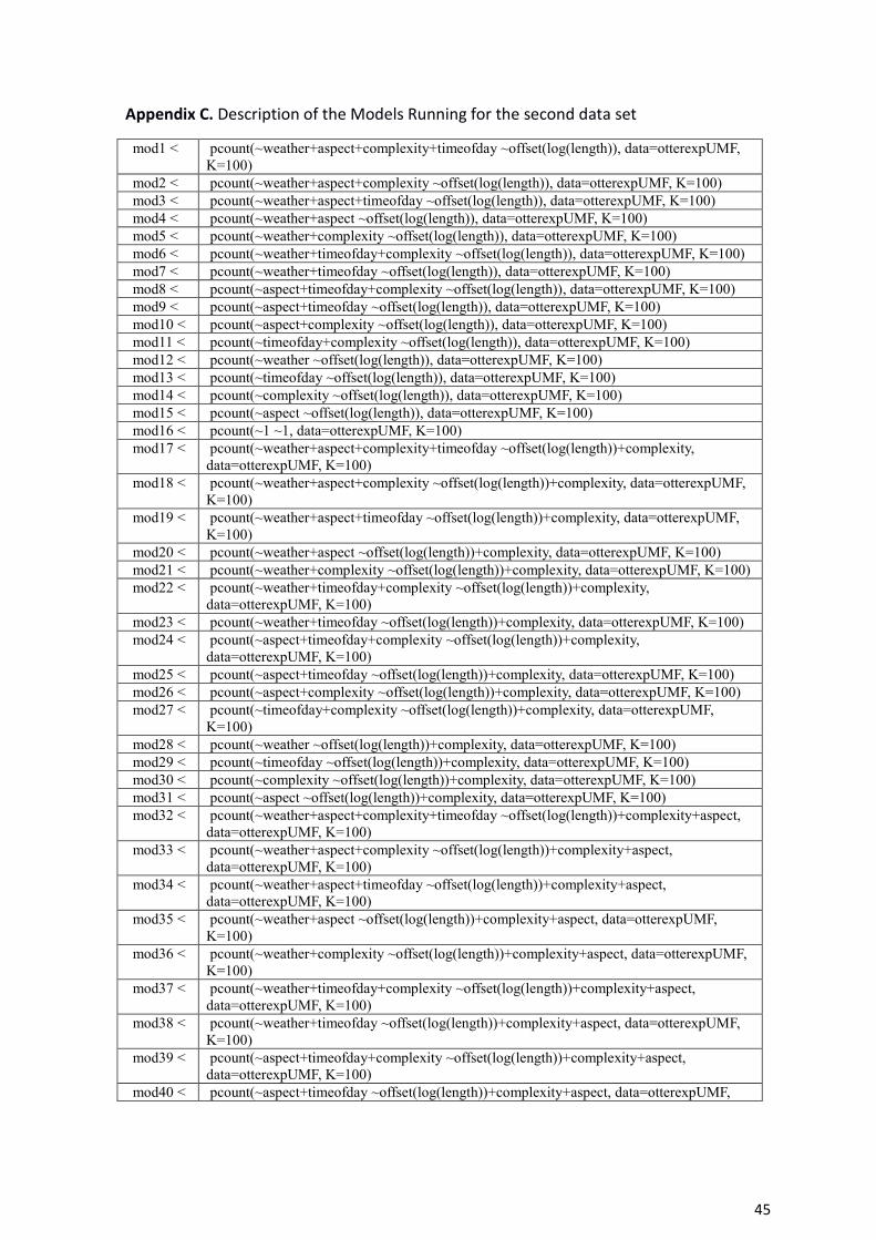
45
Appendix C. Description of the Models Running for the second data set
mod1 < pcount(~weather+aspect+complexity+timeofday ~offset(log(length)), data=otterexpUMF,
K=100)
mod2 < pcount(~weather+aspect+complexity ~offset(log(length)), data=otterexpUMF, K=100)
mod3 < pcount(~weather+aspect+timeofday ~offset(log(length)), data=otterexpUMF, K=100)
mod4 < pcount(~weather+aspect ~offset(log(length)), data=otterexpUMF, K=100)
mod5 < pcount(~weather+complexity ~offset(log(length)), data=otterexpUMF, K=100)
mod6 < pcount(~weather+timeofday+complexity ~offset(log(length)), data=otterexpUMF, K=100)
mod7 < pcount(~weather+timeofday ~offset(log(length)), data=otterexpUMF, K=100)
mod8 < pcount(~aspect+timeofday+complexity ~offset(log(length)), data=otterexpUMF, K=100)
mod9 < pcount(~aspect+timeofday ~offset(log(length)), data=otterexpUMF, K=100)
mod10 < pcount(~aspect+complexity ~offset(log(length)), data=otterexpUMF, K=100)
mod11 < pcount(~timeofday+complexity ~offset(log(length)), data=otterexpUMF, K=100)
mod12 < pcount(~weather ~offset(log(length)), data=otterexpUMF, K=100)
mod13 < pcount(~timeofday ~offset(log(length)), data=otterexpUMF, K=100)
mod14 < pcount(~complexity ~offset(log(length)), data=otterexpUMF, K=100)
mod15 < pcount(~aspect ~offset(log(length)), data=otterexpUMF, K=100)
mod16 < pcount(~1 ~1, data=otterexpUMF, K=100)
mod17 < pcount(~weather+aspect+complexity+timeofday ~offset(log(length))+complexity,
data=otterexpUMF, K=100)
mod18 < pcount(~weather+aspect+complexity ~offset(log(length))+complexity, data=otterexpUMF,
K=100)
mod19 < pcount(~weather+aspect+timeofday ~offset(log(length))+complexity, data=otterexpUMF,
K=100)
mod20 < pcount(~weather+aspect ~offset(log(length))+complexity, data=otterexpUMF, K=100)
mod21 < pcount(~weather+complexity ~offset(log(length))+complexity, data=otterexpUMF, K=100)
mod22 < pcount(~weather+timeofday+complexity ~offset(log(length))+complexity,
data=otterexpUMF, K=100)
mod23 < pcount(~weather+timeofday ~offset(log(length))+complexity, data=otterexpUMF, K=100)
mod24 < pcount(~aspect+timeofday+complexity ~offset(log(length))+complexity,
data=otterexpUMF, K=100)
mod25 < pcount(~aspect+timeofday ~offset(log(length))+complexity, data=otterexpUMF, K=100)
mod26 < pcount(~aspect+complexity ~offset(log(length))+complexity, data=otterexpUMF, K=100)
mod27 < pcount(~timeofday+complexity ~offset(log(length))+complexity, data=otterexpUMF,
K=100)
mod28 < pcount(~weather ~offset(log(length))+complexity, data=otterexpUMF, K=100)
mod29 < pcount(~timeofday ~offset(log(length))+complexity, data=otterexpUMF, K=100)
mod30 < pcount(~complexity ~offset(log(length))+complexity, data=otterexpUMF, K=100)
mod31 < pcount(~aspect ~offset(log(length))+complexity, data=otterexpUMF, K=100)
mod32 < pcount(~weather+aspect+complexity+timeofday ~offset(log(length))+complexity+aspect,
data=otterexpUMF, K=100)
mod33 < pcount(~weather+aspect+complexity ~offset(log(length))+complexity+aspect,
data=otterexpUMF, K=100)
mod34 < pcount(~weather+aspect+timeofday ~offset(log(length))+complexity+aspect,
data=otterexpUMF, K=100)
mod35 < pcount(~weather+aspect ~offset(log(length))+complexity+aspect, data=otterexpUMF,
K=100)
mod36 < pcount(~weather+complexity ~offset(log(length))+complexity+aspect, data=otterexpUMF,
K=100)
mod37 < pcount(~weather+timeofday+complexity ~offset(log(length))+complexity+aspect,
data=otterexpUMF, K=100)
mod38 < pcount(~weather+timeofday ~offset(log(length))+complexity+aspect, data=otterexpUMF,
K=100)
mod39 < pcount(~aspect+timeofday+complexity ~offset(log(length))+complexity+aspect,
data=otterexpUMF, K=100)
mod40 < pcount(~aspect+timeofday ~offset(log(length))+complexity+aspect, data=otterexpUMF,

46
K=100)
mod41 < pcount(~aspect+complexity ~offset(log(length))+complexity+aspect, data=otterexpUMF,
K=100)
mod42 < pcount(~timeofday+complexity ~offset(log(length))+complexity+aspect,
data=otterexpUMF, K=100)
mod43 < pcount(~weather ~offset(log(length))+complexity+aspect, data=otterexpUMF, K=100)
mod44 < pcount(~timeofday ~offset(log(length))+complexity+aspect, data=otterexpUMF, K=100)
mod45 < pcount(~complexity ~offset(log(length))+complexity+aspect, data=otterexpUMF, K=100)
mod46 < pcount(~aspect ~offset(log(length))+complexity+aspect, data=otterexpUMF, K=100)
mod47 < pcount(~weather+aspect+complexity+timeofday ~offset(log(length))+aspect,
data=otterexpUMF, K=100)
mod48 < pcount(~weather+aspect+complexity ~offset(log(length))+aspect, data=otterexpUMF,
K=100)
mod49 < pcount(~weather+aspect+timeofday ~offset(log(length))+aspect, data=otterexpUMF,
K=100)
mod50 < pcount(~weather+aspect ~offset(log(length))+aspect, data=otterexpUMF, K=100)
mod51 < pcount(~weather+complexity ~offset(log(length))+aspect, data=otterexpUMF, K=100)
mod52 < pcount(~weather+timeofday+complexity ~offset(log(length))+aspect, data=otterexpUMF,
K=100)
mod53 < pcount(~weather+timeofday ~offset(log(length))+aspect, data=otterexpUMF, K=100)
mod54 < pcount(~aspect+timeofday+complexity ~offset(log(length))+aspect, data=otterexpUMF,
K=100)
mod55 < pcount(~aspect+timeofday ~offset(log(length))+aspect, data=otterexpUMF, K=100)
mod56 < pcount(~aspect+complexity ~offset(log(length))+aspect, data=otterexpUMF, K=100)
mod57 < pcount(~timeofday+complexity ~offset(log(length))+aspect, data=otterexpUMF, K=100)
mod58 < pcount(~weather ~offset(log(length))+aspect, data=otterexpUMF, K=100)
mod59 < pcount(~timeofday ~offset(log(length))+aspect, data=otterexpUMF, K=100)
mod60 < pcount(~complexity ~offset(log(length))+aspect, data=otterexpUMF, K=100)
mod61 < pcount(~aspect ~offset(log(length))+aspect, data=otterexpUMF, K=100)

47
Appendix D. Results of the model selection, running for the second data set.

48
Appendix E. Covariates uses in the model of the first data set

49
Appendix F. Covariates uses in the model of the second data set