Estimate of emissions on road networks via Generic Second ...

Estimate of emissions on road networksvia Generic Second Order Models

Caterina Balzotti∗ Maya Briani§ Benedetto Piccoli‡

Abstract

In this paper we provide emission estimates due to vehicular traffic via Generic Second OrderModels. We generalize them to model road networks with merge and diverge junctions. Theprocedure consists on solving the Riemann Problem at junction assuming the maximization ofthe flow and a priority rule for the incoming roads. We provide some numerical results for asingle-lane roundabout and we propose an application of the given procedure to estimate theproduction of nitrogen oxides (NOx) emission rates. In particular, we show that the presence ofa traffic lights produces a 28% increase in the NOx emissions with respect to the roundabout.

Keywords. Second order traffic models; road networks; Riemann problem; emissions.

Mathematics Subject Classification. 35L65, 90B20, 62P12.

1 Introduction

Estimating traffic emissions is an important and challenging problem. First, emission models arebased on the knowledge of acceleration of vehicles, beside speed, thus, at macroscopic level, requiringthe use of the so-called second-order models. The latter consist of a first equation for conservationof mass and a second for the speed or momentum. The first second-order models go back to Pyaneand Whitham [22, 25], but a new of research originated starteing with the Aw-Rascle-Zhang (ARZ)model [3, 26]. The latter successfully addressed criticisms of the Payne-Whitham approach [7]. Morerecently, various models were proposed ranging from generalizations of the ARZ such as in [12, 19, 9]to phase transition models as proposed in [5, 6] and Generic Second Order Models [19, 1]. Suchmodels are characterized by a family of fundamental diagrams (density-flow graphs) and, due to theirmulti-faceted nature, they are particularly appropriate to fit real traffic data. We refer to [23, 10] formore details on data-fitted second order models.

The aim of this paper is to extend the Generic Second Order Models (GSOM) to road networks anduse it for emission estimates. Traffic models on road networks have been widely studied in recent yearsand authors have considered many different traffic scenarios proposing a rich amount of alternativejunction models. The first order Lighthill-Whitham-Richards (LWR) model [20, 24] has been extendedto road networks in several papers, see for example [15, 14, 18, 8]. In [13, 16, 17] the authors analyzethe second order ARZ model on networks.

In this paper we consider a road network with merge (two incoming and one outgoing roads) anddiverge (one incoming and two outgoing roads) junctions. On each road the traffic flow is describedby a GSOM

∂tρ+ ∂x(ρv) = 0

∂tw + v∂xw = 0,

∗Dipartimento di Scienze di Base e Applicate per l’Ingegneria, Sapienza Universita di Roma, Rome, Italy ([email protected]).§Istituto per le Applicazioni del Calcolo “M. Picone”, Consiglio Nazionale delle Ricerche, Rome, Italy

([email protected]).‡Department of Mathematical Sciences, Rutgers University, Camden, USA ([email protected]).

1

arX

iv:2

004.

1120

2v1

[ph

ysic

s.so

c-ph

] 2

0 A

pr 2

020

mailto:[email protected]




where v = V (ρ, w) is the velocity function, ρ is the density of vehicles and w is a property of drivers.We also denote y = ρw the conserved variable called total property. To define the solution on the wholenetwork we follow the approach proposed in [14] based on the concept of the Riemann Problem at ajunction, which is a Cauchy problem with constant initial data on each road connected at the junction.The idea is to solve a left-half Riemann problem (waves have non-positive speed) for incoming roadsand a right-half Riemann problem (waves have non-negative speed) for outgoing roads, defining theregion of admissible states such that waves do not enter the junction. The identification of the solutionis done by assuming the maximization of the flux and the conservation of ρ and y through the junction.The obtained maximization problem needs additional conditions depending on the considered roadnetwork to identify a unique solution. In the case of a diverge junction the unique solution is attainedby fixing a distribution parameter of the flux of vehicles among the two outgoing roads. The treatmentwe propose in this case is similar to the one proposed in [17] for the ARZ model.

For the merge junction we propose a different approach based on a priority rule for the incomingroads. We introduce the following relation between the two incoming fluxes at the junction (q+1 andq+2 ), i.e.

q+2 =β

1− βq+1 ,

for a given parameter β ∈ [0, 1]. The priority rule establishes which one of the two incoming roads atjunction sends more flow of vehicles with respect to the other road. This assumption, coupled withthe conservation of ρ and y influences the w variable. In fact, the drivers behavior of the outgoingroad w−3 is given by a convex combination of properties w+

1 and w+2 of the two incoming roads, i.e.

w−3 = (1− β)w+1 + βw+

2 .

Therefore the maximal flux that can be received by the outgoing road depends on the priority rule.We proposed a new logic to obtain a solution as follows: the flow is maximized respecting the priorityrule, but the latter can be relaxed if the outgoing road supply exceeds the demand of the road withhigher priority. This gives rise to new solutions which can describe different traffic scenarios. Forinstance, when priority is ruled by the presence of traffic lights the procedure strictly respects thepriority, while it allows the choice of the optimal parameter β in terms of flow maximization whenpriority is not strictly required as in roundabouts. The complete procedure to build the solution fora merge junction is explained in details in Definition 4.1.

To numerically test the proposed method, we use the Collapsed Generalized Aw-Rascle-Zhang(CGARZ) model [11], which fits in the framework of GSOM. Following [4] we specify as fundamentaldiagram a convex combination of the Newell-Daganzo or triangular fundamental diagram with theGreenshield quadratic one. We then analyze the case of a merge and diverge junction and we combinethem to build a simple roundabout. Finally we propose an application of the traffic theory to estimatethe nitrogen oxides (NOx) emissions due to vehicular traffic. The interest on NOx gases is due to theirnegative effects on health [27] and to their connection to ozone [2]. Here we extend the results obtainedin [4] to a road network. In particular, we analyze the impact produced by the presence of trafficlights on the incoming roads into the roundabout, comparing the emission rates produced with andwithout them. The numerical tests show the great impact that traffic lights have on NOx emissionrates, resulting in a 28% increase compared to emissions without traffic lights. This procedure can beapplied to any other pollutant associated to vehicle traffic.

The paper is organized as follows. In Section 2 we introduce the GSOM and in Section 3 theRiemann problem at junction. In Section 4 we define the solution to the Riemann problem forjunctions with one incoming road and one outgoing road, one incoming road and two outgoing roadsand two incoming roads and one outgoing road. In Section 5 we show some numerical tests and inSection 6 we apply the proposed model to estimate NOx emissions.

2

2 Traffic model

In this work we extend the Generic Second Order Models (GSOM) [19] to road networks. We denote byGSOM a family of macroscopic traffic models which are described by a first order Lighthill-Whitham-Richards (LWR) model [20, 24] with variable fundamental diagrams. Such models are defined by

∂tρ+ ∂x(ρv) = 0

∂tw + v∂xw = 0

with v = V (ρ, w),

(2.1)

where ρ(x, t), v(x, t) and w(x, t) represent the density, the speed and a property of vehicles advectedby the flow, respectively, and V is a specific velocity function. The first equation of (2.1) is theconservation of vehicles, the second one is the advection of the attribute of drivers, which definestheir driving aptitude by means of different fundamental diagrams. Indeed, the variable w identifiesthe flux curve Q(ρ, w) and thus the speed of vehicles V (ρ, w) = Q(ρ, w)/ρ which characterizes thebehavior of drivers. System (2.1) is written in conservative form as

∂tρ+ ∂x(ρv) = 0

∂ty + ∂x(yv) = 0

with v = V(ρ,y

ρ

),

(2.2)

where y = ρw denotes the total property of vehicles.The flux function Q(ρ, w) and the velocity function V (ρ, w) = Q(ρ, w)/ρ are assumed to satisfy

the following properties.

(H1) Q(ρ, w) is strictly concave with respect to ρ, i.e. ∂2Q∂ρ2 < 0.

(H2) Q(0, w) = 0 and Q(ρmax, w) = 0 for each w ∈ [wL, wR], where ρmax is the maximum density ofvehicles and [wL, wR] is the domain of w, for suitable wL and wR.

(H3) Q(ρ, w) is non-decreasing with respect to w, i.e. ∂Q∂w ≥ 0.

(H4) V (ρ, w) ≥ 0 for each w.

(H5) V (ρ, w) is strictly decreasing with respect to ρ, i.e. ∂V∂ρ < 0 for each w.

(H6) V (ρ, w) is non-decreasing with respect to w, i.e. ∂V∂w ≥ 0.

Note that property (H5) is a consequence of the concavity (H1) and that (H6) is a consequence of(H3). Properties (H1) and (H2) imply that the flux curve Q(·, w) has a unique point of maximumfor any w. We denote by σ(w) the critical density, i.e. the density value where the flux attends itsmaximum Qmax(w). Moreover, for any ρ there exists a unique ρ(w) such that Q(ρ, w) = Q(ρ(w), w).

We recall now the main definitions concerning traffic models on road networks and we refer to[8, 14, 15, 18] for further details. Let us consider a junction J with n incoming and m outgoing roadsIr = [ar, br] ⊂ R, r = 1, . . . , n+m, possibly with ar = −∞ and br = +∞. We define a network as acouple (I,J ) where I is a finite collection of roads Ir, and J is a finite collection of junctions J .

On each road Ir, r = 1, . . . , n+m, the traffic dynamic is described by a GSOM (2.2) as∂tρr + ∂x(ρrvr) = 0

∂tyr + ∂x(yrvr) = 0

with vr = V

(ρr,

yrρr

),

(2.3)

3

for x ∈ Ir and t ≥ 0. Following [17, 18], we consider a set of smooth test functions φr : Ir× [0,+∞)→R2 with compact support in Ir = [ar, br] which are smooth also across each junction J , i.e.

φi(bi) = φj(aj) and ∂xφi(bi) = ∂xφj(aj) (2.4)

for i = 1, . . . , n and j = n + 1, . . . ,m. We define a weak solution of (2.3) as a couple of functions(ρr(x, t), yr(x, t)) which satisfy

n+m∑r=1

(∫ ∞0

∫ br

ar

(ρr(x, t)∂tφr(x, t) + (ρr(x, t)vr(x, t))∂xφr(x, t))dxdt+

∫ br

ar

ρr(x, 0)φr(x, 0)dx

)= 0

n+m∑r=1

(∫ ∞0

∫ br

ar

(yr(x, t)∂tφr(x, t) + (yr(x, t)vr(x, t))∂xyr(x, t))dxdt+

∫ br

ar

yr(x, 0)φr(x, 0)dx

)= 0

(2.5)

for all the test functions φr satisfying (2.4), where (ρr(x, 0), yr(x, 0)) is the initial data.The construction of weak solutions in the sense of (2.5) is explained in detail in the following

sections and it depends on the type of junction: we solve the Riemann problem for (2.3) on each roadr with the following initial data

(ρr(x, 0), yr(x, 0)) =

(ρ−, y−) for x < x0

(ρ+, y+) for x > x0,(2.6)

where only one between the left and right state is known. Depending on Ir if it is an incoming or anoutgoing road, we have the following possibilities:

• If Ir is an incoming road at junction then x0 = br and only the left state (ρ−, y−) is known. Inthis case we look for weak solutions of (2.3) such that the waves have non-positive speed.

• If Ir is an outgoing road at junction then x0 = ar and only the right state (ρ+, y+) is known.In this case we look for weak solutions of (2.3) such that the waves have non-negative speed.

The construction of a unique solution is performed by means of the maximization of the flux, as itwill be clearer in the following sections.

3 Preliminaries for the Riemann problem at junction

As a first step, we study the properties of the traffic model (2.2). For convenience, we introduce thevariable

u = u(ρ, y) = V

(ρ,y

ρ

), (3.1)

and we rewrite the system as ∂tρ+ ∂x(ρu) = 0

∂ty + ∂x(yu) = 0,(3.2)

whose Jacobian is

DF (ρ, y) =

(u+ ρuρ ρuyyuρ u+ yuy

). (3.3)

Since it is easier to work with the couple (ρ, w), hereafter we will use these variables. The eigenvaluesof (3.3), as a function of (ρ, w), are

λ1(ρ, w) = V (ρ, w) + ρVρ(ρ, w) (3.4)

λ2(ρ, w) = V (ρ, w). (3.5)

4

By property (H5) follows λ1 ≤ λ2 and λ1 = λ2 if and only if ρ = 0, thus the system is strictlyhyperbolic except for ρ = 0.

The eigenvectors associated to the eigenvalues are

γ1(ρ, w) = (ρ, ρw) (3.6)

γ2(ρ, w) =

(−1

ρVw(ρ, w), Vρ(ρ, w)− 1

ρ2Vw(ρ, w)

). (3.7)

The first eigenvalue is genuinely nonlinear, i.e. ∇λ1 ·γ1 6= 0, while the second one is linearly degenerate,i.e. ∇λ2 · γ2 = 0. Hence, the curve of the first family are 1-shocks or 1-rarefaction waves, while thecurve of the second family are 2-contact discontinuities.

Finally the Riemann invariants are

z1(ρ, w) = w (3.8)

z2(ρ, w) = V (ρ, w). (3.9)

The 1-shock and 1-rarefaction waves are defined by the first Riemann invariant z1 and the 2-contactdiscontinuities by the second Riemann invariant z2.

Remark 3.1. All the Figures shown hereafter refer to a particular GSOM, the Collapsed GeneralizedAw-Rascle-Zhang (CGARZ) model with the family of flux functions defined in Section 5.

In order to construct waves with non-negative or non-positive speed at junction, we study the signof the eigenvalues defined in (3.4) and (3.5). The first eigenvalue λ1(ρ, w) = ρ+ ρVρ(ρ, w) = Qρ(ρ, w)is such that λ1 ≥ 0 for ρ ≤ σ(w) and λ1 < 0 for ρ > σ(w), by properties (H1) and (H2) of the fluxfunction. Hence, for each w ∈ [wL, wR] the 1-shocks and 1-rarefaction waves have non-negative speedfor ρ ≤ σ(w) and negative speed for ρ > σ(w). In Figure 1 we show an example of the positive andnegative regions of λ1 obtained with the flux and velocity functions defined in Section 5. The secondeigenvalue λ2(ρ, w) = V (ρ, w) ≥ 0 by definition of V , thus the speed of the 2-contact discontinuitiesis always non-negative.

Figure 1. Example of positive (yellow-down) and negative (green-up) regions for λ1 depending on w.

In order to maximize the flux in the following sections we will make use of the supply and demandfunctions. For each w ∈ [wL, wR], the supply function s(ρ, w) is defined as

s(ρ, w) =

Qmax(w) if ρ ≤ σ(w)

Q(ρ, w) if ρ > σ(w).(3.10)

5

Analogously, we define the demand function d(ρ, w) as

d(ρ, w) =

Q(ρ, w) if ρ ≤ σ(w)

Qmax(w) if ρ > σ(w).(3.11)

In Figure 2 we show an example of the supply function on the left and of the demand function on theright.

Figure 2. Supply function (left) and demand function (right).

3.1 Incoming road at the junction

Let us consider an incoming road at the junction. We are then interested only in the waves withnon-positive speed. Since λ2 ≥ 0, we can just have 1-shock or 1-rarefaction waves. Let us fix a leftstate U− = (ρ−, w−), our aim is to define the set of all possible right states U+ = (ρ+, w+) that canbe connected to U− with a wave with non-positive speed. We denote by N (U−) the set of admissibledensities.

Proposition 3.1. Let U− = (ρ−, w−) be a left state on an incoming road. The set of possibile rightstates U+ = (ρ+, w+) that can be connected to the left state lies on the level curve z1 = w−, i.e.w+ = w−, and they are such that:

1. If ρ− ≤ σ(w−), then ρ+ must be in N (U−) = [ρ−(w−), ρmax], where ρ−(w−) is the density suchthat Q(ρ−(w−), w−) = Q(ρ−, w−).

2. If ρ− > σ(w−), then ρ+ must be in N (U−) = [σ(w−), ρmax].

The proof of the previous proposition is analogous to the one proposed in [17], where the authorsstudy the Riemann problem on a network for the Aw-Rascle model, which belongs to the GSOM. InFigure 3 we show an example of the two possibile states configurations at incoming road.

Remark 3.2. We observe that the flux of the right state satisfies

Q(ρ+, w+) ≤ d(ρ−, w−), (3.12)

where d is the demand function defined in (3.11). Indeed, if ρ− ≤ σ(w−) then ρ+ must be inN (U−) = [ρ−(w−), ρmax], where the flux is lower than or equal to Q(ρ−, w−); if ρ− > σ(w−), then ρ+

must be in N (U−) = [σ(w−), ρmax], where the flux is lower than Qmax(w−). These two possibilitiesare summarized in (3.12).

6

Figure 3. Two possible configurations of incoming road states. The red segment identifies the set of possibleright states U+ = (ρ+, w+) reachable from the left state U−.

3.2 Outgoing road at the junction

Let us consider an outgoing road at the junction. We are interested in the waves with non-negativespeed, thus we can have a 1-shock or 1-rarefaction wave and a 2-contact discontinuity. Let us fixa right state U+ = (ρ+, w+), our aim is to define the set of all possible left states U− = (ρ−, w−)that can be connected to U+ with waves with non-negative speed. We denote by P(U†) the set ofadmissible densities.

Proposition 3.2. Let U+ = (ρ+, w+) be a right state on an outgoing road, and v+ the associatedvelocity V (ρ+, w+). Let U† = (ρ†, w†) be the intersection point between the level curves z2 = v+and z1 = c, for a certain c, with ρ† = ρ†(v+, c) and w† = c. The set of possibile left statesU− = (ρ−, w−) that can be connected to the right state are such that w− = c and

1. If ρ† ≤ σ(w+), then ρ− must be in P(U+) = [0, σ(w†)].

2. If ρ† > σ(w+), then ρ− must be in P(U+) = [0, ρ†(w†))∪ρ†, where ρ†(w†) is the density suchthat Q(ρ†(w†), w†) = Q(ρ†, w†).

Again, we refer to [17] for the details of the proof. In Figure 4 we show an example of the twopossibile states configurations at outgoing road.

Remark 3.3. We observe that w† = w− = c and that the flux of the left state satisfies

Q(ρ−, w−) ≤ s(ρ†, w†), (3.13)

where s is the supply function defined in (3.10). Indeed, if ρ† ≤ σ(w+) then ρ− must be in P(U+) =[0, σ(w†)], where the flux is lower than or equal to Qmax(w†); if ρ† > σ(w+), then ρ− must bein P(U+) = [0, ρ†(w†)) ∪ ρ†, where the flux is lower than Q(ρ†, w†). These two possibilities aresummarized in (3.13).

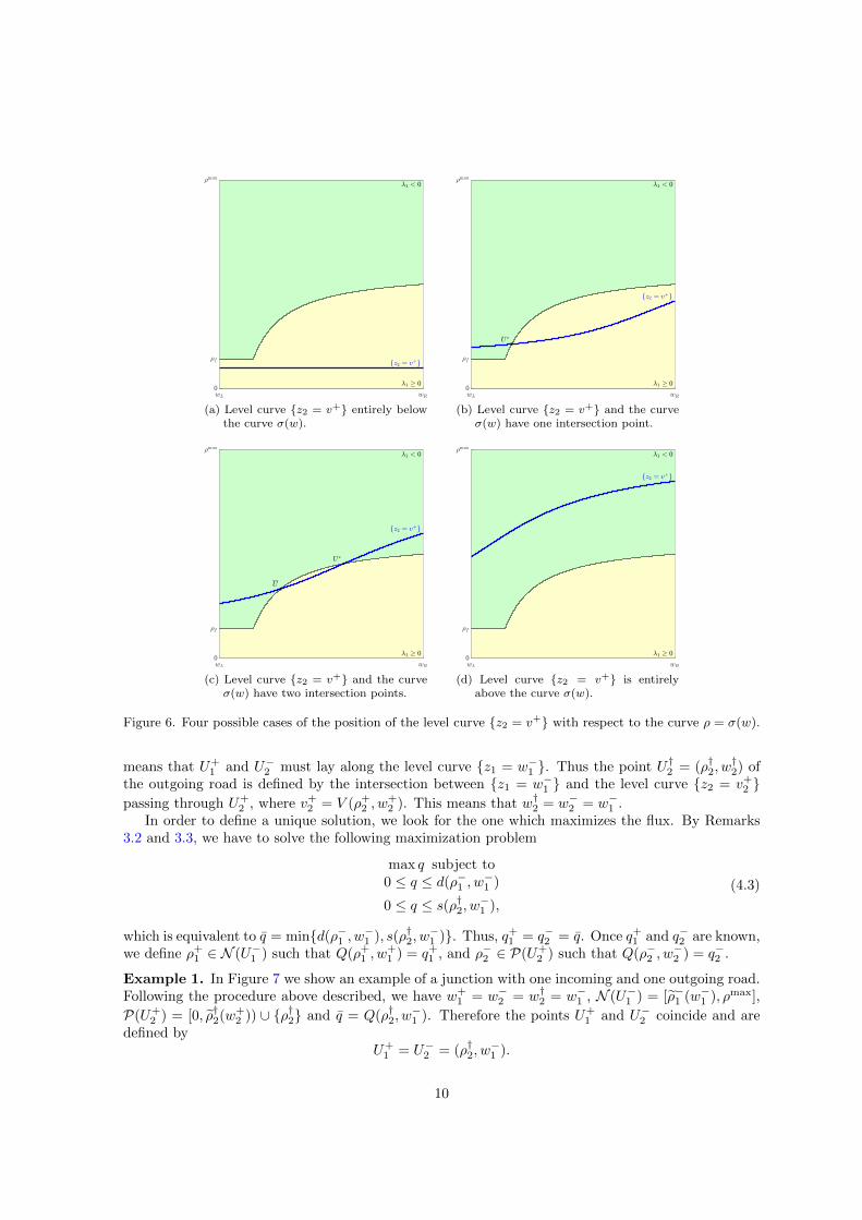
We focus now on the intersection point U† between the level curves of the two Riemann invariantsz1 = w− and z2 = v+, for a certain w− and v+. In the propositions which follow, we referto Figures 5 and 6, whose plots are obtained with the CGARZ model and flux functions defined inSection 5. However, the statements of Propositions 3.3 and 3.4 hold for any GSOM with flux andvelocity functions satisfying properties (H1)-(H6).

7

Figure 4. Two possible configurations of outgoing road. The red segment identifies the set of possible leftstates U− = (ρ−, w−) reachable from the left state U+.

Proposition 3.3. Let V be a velocity function verifying hypotheses (H5) and (H6), the followingstatements hold.

1. The intersection point U† = (ρ†, w†) is such that w† = w− and ρ†(v−, w−) is the unique densityvalue such that V (ρ†, w−) = v+.

2. The function ρ†(v−, w) is non-decreasing in w.

Proof. We have w† = w− by construction, while the uniqueness of ρ† follows by the property (H5) ofthe velocity function V . To prove the monotonicity of ρ†, let us consider the family of speed functionsV (ρ, w) (see for example the left plot of Figure 5). If we cut the speed-family with a horizontal lineV = v+, we obtain the density values whose velocity is equal to v+ as w changes. By property(H6) follows that ρ is non-decreasing in w, thus the level curve z2 = v+ is non-decreasing in the(w, ρ)-plane, see the right plot of Figure 5. Since ρ† lies on these curves the thesis follows.

Figure 5. Example of family of speed functions (left) and level curves of ρ† for different values of v+ (right).

8

Proposition 3.4. For any v+ ∈ [0, V max] and w ∈ [wL, wR] the function s(ρ†, w) (3.10) is non-decreasing in w, where ρ† = ρ†(v+, w) is the density of the intersection point between the level curvesof the two Riemann invariants z1 = w and z2 = v+.

Proof. First of all we observe that all the points ρ† along the level curve z2 = v+ are such thatQ(ρ†, w) = v+ρ†, for any w ∈ [wL, wR]. Since ρ† is non-decreasing in w by Proposition 3.3, also theflux along the curve is non-decreasing in w. We divide the proof in four cases.

1. The level curve z2 = v+ is entirely below the curve ρ = σ(w), see Figure 6(a). In this case wehave s(ρ†, w) = Qmax(w), which is non-decreasing in w by property (H3).

2. The level curve z2 = v+ has a unique intersection point with the curve ρ = σ(w), see Figure6(b). In this case, denoting by U∗ = (w∗, ρ∗) the intersection point, we have

s(ρ†, w) =

v+ρ† if w ≤ w∗

Qmax(w) if w > w∗,

which is non-decreasing in w by Proposition 3.3 and property (H3).

3. The level curve z2 = v+ has two intersection points with the curve ρ = σ(w), see Figure6(c). We denote by U = (w, ρ) and U∗ = (w∗, ρ∗) the first and the second intersection point,respectively. We have

s(ρ†, w) =

v+ρ† if w ≤ wQmax(w) if w < w ≤ w∗

v+ρ† if w > w∗.

We observe that we recover the previous case for the points U = (w, ρ) such that w ≤ w∗. SinceU∗ intersects σ(w), we have Q(ρ∗, w∗) = Qmax(w∗) = v+ρ∗. For any δ, ε > 0, if (w+ δ, ρ∗+ ε) ∈z2 = v+ then Q(ρ∗ + ε, w∗ + δ) = v+(ρ∗ + ε) > Q(ρ∗, w∗), thus the supply function is alwaysnon-decreasing also for w > w∗.

4. The level curve z2 = v+ is entirely above the curve ρ = σ(w), see Figure 6(d). In this case wehave s(ρ†, w) = v+ρ†, which is non-decreasing in w by Proposition 3.3.

4 The GSOM on networks

In this work we deal with road networks characterized by simple junctions. Specifically, we definethe solution for junctions with one incoming road and one outgoing road, one incoming road and twooutgoing roads and two incoming roads and one outgoing road.

4.1 One incoming and one outgoing road at junction

We consider the simplest case of two roads connected by a junction. We have a left state U−1 for theincoming road and a right state U+

2 for the outgoing road and we have to solve the Riemann problemat the junction. Thus, our aim is to recover U+

1 and U−2 .We assume that ρ and y are conserved at the junction, i.e.

ρ+1 v+1 = ρ−2 v

−2 (4.1)

ρ+1 v+1 w

+1 = ρ−2 v

−2 w−2 . (4.2)

Equation (4.1) implies that q+1 = q−2 , therefore equation (4.2) implies w+1 = w−2 . Since w is the first

Riemann invariant, by the preliminary studies on the incoming road we have w−1 = w+1 = w−2 . This

9

(a) Level curve z2 = v+ entirely belowthe curve σ(w).

(b) Level curve z2 = v+ and the curveσ(w) have one intersection point.

(c) Level curve z2 = v+ and the curveσ(w) have two intersection points.

(d) Level curve z2 = v+ is entirelyabove the curve σ(w).

Figure 6. Four possible cases of the position of the level curve z2 = v+ with respect to the curve ρ = σ(w).

means that U+1 and U−2 must lay along the level curve z1 = w−1 . Thus the point U†2 = (ρ†2, w

†2) of

the outgoing road is defined by the intersection between z1 = w−1 and the level curve z2 = v+2 passing through U+

2 , where v+2 = V (ρ+2 , w+2 ). This means that w†2 = w−2 = w−1 .

In order to define a unique solution, we look for the one which maximizes the flux. By Remarks3.2 and 3.3, we have to solve the following maximization problem

max q subject to0 ≤ q ≤ d(ρ−1 , w

−1 )

0 ≤ q ≤ s(ρ†2, w−1 ),

(4.3)

which is equivalent to q = mind(ρ−1 , w−1 ), s(ρ†2, w

−1 ). Thus, q+1 = q−2 = q. Once q+1 and q−2 are known,

we define ρ+1 ∈ N (U−1 ) such that Q(ρ+1 , w+1 ) = q+1 , and ρ−2 ∈ P(U+

2 ) such that Q(ρ−2 , w−2 ) = q−2 .

Example 1. In Figure 7 we show an example of a junction with one incoming and one outgoing road.Following the procedure above described, we have w+

1 = w−2 = w†2 = w−1 , N (U−1 ) = [ρ−1 (w−1 ), ρmax],

P(U+2 ) = [0, ρ†2(w+

2 )) ∪ ρ†2 and q = Q(ρ†2, w−1 ). Therefore the points U+

1 and U−2 coincide and aredefined by

U+1 = U−2 = (ρ†2, w

−1 ).

10

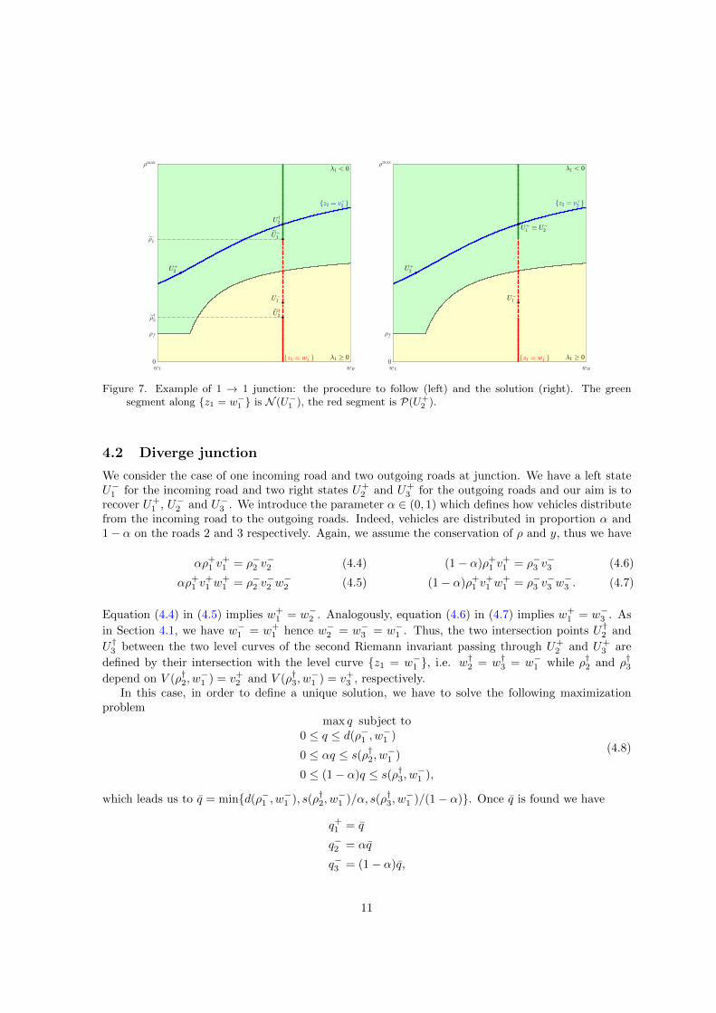
Figure 7. Example of 1 → 1 junction: the procedure to follow (left) and the solution (right). The greensegment along z1 = w−1 is N (U−1 ), the red segment is P(U+

2 ).

4.2 Diverge junction

We consider the case of one incoming road and two outgoing roads at junction. We have a left stateU−1 for the incoming road and two right states U+

2 and U+3 for the outgoing roads and our aim is to

recover U+1 , U−2 and U−3 . We introduce the parameter α ∈ (0, 1) which defines how vehicles distribute

from the incoming road to the outgoing roads. Indeed, vehicles are distributed in proportion α and1− α on the roads 2 and 3 respectively. Again, we assume the conservation of ρ and y, thus we have

αρ+1 v+1 = ρ−2 v

−2 (4.4)

αρ+1 v+1 w

+1 = ρ−2 v

−2 w−2 (4.5)

(1− α)ρ+1 v+1 = ρ−3 v

−3 (4.6)

(1− α)ρ+1 v+1 w

+1 = ρ−3 v

−3 w−3 . (4.7)

Equation (4.4) in (4.5) implies w+1 = w−2 . Analogously, equation (4.6) in (4.7) implies w+

1 = w−3 . As

in Section 4.1, we have w−1 = w+1 hence w−2 = w−3 = w−1 . Thus, the two intersection points U†2 and

U†3 between the two level curves of the second Riemann invariant passing through U+2 and U+

3 are

defined by their intersection with the level curve z1 = w−1 , i.e. w†2 = w†3 = w−1 while ρ†2 and ρ†3depend on V (ρ†2, w

−1 ) = v+2 and V (ρ†3, w

−1 ) = v+3 , respectively.

In this case, in order to define a unique solution, we have to solve the following maximizationproblem

max q subject to0 ≤ q ≤ d(ρ−1 , w

−1 )

0 ≤ αq ≤ s(ρ†2, w−1 )

0 ≤ (1− α)q ≤ s(ρ†3, w−1 ),

(4.8)

which leads us to q = mind(ρ−1 , w−1 ), s(ρ†2, w

−1 )/α, s(ρ†3, w

−1 )/(1− α). Once q is found we have

q+1 = q

q−2 = αq

q−3 = (1− α)q,

11

and then we define ρ+1 ∈ N (U−1 ) such that Q(ρ+1 , w+1 ) = q+1 , ρ−2 ∈ P(U+

2 ) such that Q(ρ−2 , w−2 ) = q−2

and ρ−3 ∈ P(U+3 ) such that Q(ρ−3 , w

−3 ) = q−3 .

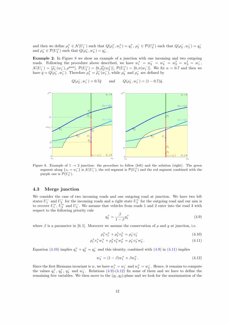
Example 2. In Figure 8 we show an example of a junction with one incoming and two outgoingroads. Following the procedure above described, we have w+

1 = w−2 = w−3 = w†2 = w†3 = w−1 ,

N (U−1 ) = [ρ−1 (w−1 ), ρmax], P(U+2 ) = [0, ρ†2(w+

2 )], P(U+3 ) = [0, σ(w−1 )]. We fix α = 0.7 and then we

have q = Q(ρ−1 , w−1 ). Therefore ρ+1 = ρ−1 (w−1 ), while ρ−2 and ρ−3 are defined by

Q(ρ−2 , w−1 ) = 0.7q and Q(ρ−3 , w

−1 ) = (1− 0.7)q.

Figure 8. Example of 1 → 2 junction: the procedure to follow (left) and the solution (right). The greensegment along z1 = w−1 is N (U−1 ), the red segment is P(U+

2 ) and the red segment combined with thepurple one is P(U+

3 ).

4.3 Merge junction

We consider the case of two incoming roads and one outgoing road at junction. We have two leftstates U−1 and U−2 for the incoming roads and a right state U+

3 for the outgoing road and our aim isto recover U+

1 , U+2 and U−3 . We assume that vehicles from roads 1 and 2 enter into the road 3 with

respect to the following priority rule

q+2 =β

1− βq+1 (4.9)

where β is a parameter in [0, 1]. Moreover we assume the conservation of ρ and y at junction, i.e.

ρ+1 v+1 + ρ+2 v

+2 = ρ−3 v

−3 (4.10)

ρ+1 v+1 w

+1 + ρ+2 v

+2 w

+2 = ρ−3 v

−3 w−3 . (4.11)

Equation (4.10) implies q+1 + q+2 = q−3 and this identity, combined with (4.9) in (4.11) implies

w−3 = (1− β)w+1 + βw+

2 . (4.12)

Since the first Riemann invariant is w, we have w+1 = w−1 and w+

2 = w−2 . Hence, it remains to computethe values q+1 , q+2 , q−3 and w−3 . Relations (4.9)-(4.12) fix some of them and we have to define theremaining free variables. We then move to the (q1, q2)-plane and we look for the maximization of the

12

flow. Therefore, we introduce d1 = d(ρ−1 , w−1 ), d2 = d(ρ−2 , w

−2 ) and the rectangle Ω = [0, d1]× [0, d2],

and we focus on the intersection point between the straight lines

r : q2 =β

1− βq1 (4.13)

s : q2 = s3 − q1, (4.14)

where s3 = s(ρ†3, w−3 ). Note that s3 = s3(β), since both ρ†3 and w−3 depend on β. The intersection

point isP = ((1− β)s3, βs3). (4.15)

In the following we define U+1 , U+

2 and U−3 .

Definition 4.1. Assuming (4.10) and (4.12) we define first the two values q+1 and q+2 which dependon the position of the intersection point P and then the other variables.

i. Procedure to set the incoming fluxes q+1 and q+2 .

1. The point P is inside the rectangle, i.e.(1− β)s3 ≤ d1βs3 ≤ d2,

see Figure 9(a). In this case the point P identifies q+1 = (1− β)s3 and q+2 = βs3.

2. The point P is to the right of the rectangle, i.e.(1− β)s3 > d1

βs3 ≤ d2,

see Figure 9(b). We have the following possibilities:

(a) If we need to respect the priority rule, then the incoming fluxes must be on the straightline r, thus the point Q in Figure 9(b) identifies q+1 = d1 and q+2 = βd1/(1− β).

(b) If there exists a β > β such that the intersection point between the correspondingstraight lines r and s crosses the rectangle in d1, as the point R in Figure 9(b), then

that point defines q+1 = d1, q+2 = βs3(β) and w−3 = (1− β)w−1 + βw−2 . Otherwise the

point S in Figure 9(b) identifies q+1 = d1, q+2 = d2 and w−3 = (1− β)w−1 + βw−2 , where

β = d2/(d1 + d2).

3. The point P is above the rectangle, i.e.(1− β)s3 ≤ d1βs3 > d2.

see Figure 9(c). We have the following possibilities:

(a) If we need to respect the priority rule, then the incoming fluxes must be on the straightline r, thus the point Q in Figure 9(c) identifies q+1 = (1− β)d2/β and q+2 = d2.

(b) If there exists a β < β such that the intersection point between the correspondingstraight lines r and s crosses the rectangle in d2, as the point R in Figure 9(c), then

that point defines q+1 = (1− β)s3(β), q+2 = d2 and w−3 = (1− β)w−1 + βw−2 . Otherwise

the point S in Figure 9(c) identifies q+1 = d1, q+2 = d2 and w−3 = (1 − β)w−1 + βw−2 ,

where β = d2/(d1 + d2).

13

4. The point P is completely outside the rectangle, i.e.(1− β)s3 > d1

βs3 > d2,

see Figure 9(d). In this case, if we need to respect the priority rule we recover the case 2(a)or 3(a), depending on β. Otherwise we recover the case 2(b) or 3(b), depending on β.

ii. We obtain q−3 = q+1 + q+2 and we define ρ+1 ∈ N (U−1 ) such that Q(ρ+1 , w+1 ) = q+1 , ρ+2 ∈ N (U−2 )

such that Q(ρ+2 , w+2 ) = q+2 and ρ−3 ∈ P(U+

3 ) such that Q(ρ−3 , w−3 ) = q−3 .

(a) Point P inside the rectangle. The solu-tion is the point P .

(b) Point P on the right of the rectangle.The solution is the point Q, R or S.

(c) Point P above the rectangle. The solu-tion is the point Q, R or S.

(d) Point P completely outside the rectan-gle. We recover the case 2 or 3.

Figure 9. The four possible positions of the point P with respect to the rectangle Ω.

Proposition 4.1. The values U+1 , U+

2 and U−3 given in Definition 4.1 are uniquely defined.

Proof. We have that the angle between the straight line r and the x-axis of the (q1, q2)-plane alwaysincreases with β. The straight line s, instead, moves to the bottom if w−1 > w−2 and to the top ifw−1 ≤ w

−2 . Indeed, in the first case w−3 decreases with β and, as consequence of Proposition 3.4, s3 is

non-increasing, while in the second case w−3 increases with β and s3 is non-decreasing.

14

Therefore, by the monotonicity of s3 the procedure described above identifies a unique couple ofvalues (q+1 ,q+2 ) and consequently the solution U+

1 , U+2 and U−3 is uniquely defined.

Example 3. In Figure 10 we show an example of a junction with two incoming and one outgoingroads. Following the procedure above described, we fix β = 0.6 and we have w+

1 = w−1 , w+2 = w−2 ,

w+3 = (1 − β)w−1 + βw−2 , N (U−1 ) = [σ(ρ−1 ), ρmax], N (U−2 ) = [ρ†2(w−2 ), ρmax], P(U+

3 ) = [0, σ(w−3 )].The point P of intersection between the straight lines r and s is inside the rectangle Ω, thus q+1 =(1 − β)s3(β), q+2 = βs3(β) and q−3 = s3(β). Finally we compute the densities ρ+1 , ρ+2 and ρ−3 suchthat q+1 = Q(ρ+1 , w

+1 ), q+2 = Q(ρ+2 , w

+2 ) and q−3 = Q(ρ−3 , w

−3 ), as shown in the right plot of Figure 10.

Figure 10. Example of 2→ 1 junction: the procedure to follow (left) and the solution (right).

Remark 4.1. The solution proposed in [17] can be recovered by fixing β = 0.5 in our procedure.

Remark 4.2. Let us consider the particular case of w constant in all the roads. The 1 → 1 and1→ 2 junctions can be treated exactly as the LWR model at junction, as done in [14]. For the 2→ 1junction we observe that the assumption of w constant implies that the straight line s defined in (4.14)coincides for all β, therefore the solution is limited to the points P or Q, excluding the points R or S.Thus, we recover again the LWR model on networks, as treated in [14].

5 Numerical simulations

In this section we show some numerical tests to simulate the solution for different types of junction.We consider the traffic model on a network with roads Ir = [ar, br] during a time interval [0, T ]. Wedivide each road into Nx + 1 cells of length ∆x, and the time interval into Nt + 1 steps of length∆t. We choose the CGARZ model among the family of GSOM, which is numerically solved with the2CTM scheme [11] with suitable boundary conditions on the cells which are at the extremes of thenetwork. Depending on the type of junction we use the theory defined in Sections 4.1, 4.2 and 4.3 tocompute the density and the property of vehicles w on the junction boundary cells, which are denotedby ρJr and wJr respectively, for each road r.

The CGARZ model assumes that flux of vehicles is not influenced by w when the density value islower than a certain threshold. Thus, the flux of the CGARZ model is described by a single-valuedfundamental diagram in free-flow regimes, and by a multi-valued function in congestion. The flux

15

function is then defined by

Q(ρ, w) =

Qf (ρ) if 0 ≤ ρ ≤ ρfQc(ρ, w) if ρf < ρ ≤ ρmax,

(5.1)

where ρf is the free-flow threshold density and ρmax is the maximum density. Following [4], we assumethat the flux function is described by the Greenshields model in the free-flow phase, i.e.

Qf (ρ) =V max

ρmaxρ (ρmax − ρ) , (5.2)

and by a convex combination of a lower-bound function f(ρ) and an upper-bound function g(ρ) inthe congested phase. In particular, we set

f(ρ) =V max

ρmaxρf (ρmax − ρ) (5.3)

g(ρ) =V max

ρmaxρ (ρmax − ρ) . (5.4)

We define

θ(w) =w − wLwR − wL

, (5.5)

with wL = Qf (ρf ) and wR = Qf (ρmax/2), where ρmax/2 is the critical density of Qf (·). Note thatthis means that w identifies the maximum reachable flux by the flux function.

The flux function in the congested phase Qc(ρ, w) is then defined by

Qc(ρ, w) = (1− θ(w))f(ρ) + θ(w)g(ρ), (5.6)

with f and g given in (5.3) and (5.4). The velocity function is

V (ρ, w) =Q(ρ, w)

ρ. (5.7)

In all the tests which follow we fix these parameters: ρf = 19 veh/km, ρmax = 133 veh/km,V max = 120 km/h, L = 1 km, T = 2 min, ∆x = 0.02 km, ∆t = 0.3 s, wL = 1954 and wR = 3990.

5.1 The case of 1→1 junction

Let us consider two roads connected by a junction, as depicted in Figure 11. We denote by ρn1,j =ρ1(xj , t

n) the density of road 1, and by ρn2,j = ρ2(xj , tn) the density of road 2, for j = 0, . . . , Nx and

n = 0, . . . , Nt. We use the 2CTM scheme to compute the density on the nodes inside the roads, i.e.ρn1,j for j = 0, . . . , Nx − 1 and ρn2,j for j = 1, . . . , Nx. The junction is treated as a boundary ghost cell

and densities ρn1,Nx= ρJ1 and ρn2,0 = ρJ2 are computed as explained in Section 4.1.

1 2

J

Figure 11. Example of 1→ 1 junction.

In the following test the couple (ρ0r,·, w0r,·) of the two roads is taken as in Table 1. The density at

the left boundary of road 1 is fixed to ρn1,0 = 50 veh/km for any time and the right boundary of road2 is such that vehicles are free to leave the road. Figure 12 shows the evolution of traffic in time. Atthe beginning the dynamic of the first road is described by a shock wave which moves backwards untilit moves to a rarefaction wave, while the vehicles enter into the second road with a rarefaction wave.Note that, the dynamic of road 2 is slowed down by its lower value of w with respect to road 1, whichimposes vehicles to have a slower velocity.

16

Road r ρ0r,j (veh/km) w0r,·

150 j ≤ Nx/2

wR100 j > Nx/2

2 70∀ j wL

Table 1. Initial data for the 1→ 1 junction.

0 0.5 1 1.5 2

Space (km)

0

20

40

60

80

100

120

Density (

veh/k

m)

(a) Density at time t = 0.

0 0.5 1 1.5 2

Space (km)

0

20

40

60

80

100

120

Density (

veh/k

m)

(b) Density at time t = T/4.

0 0.5 1 1.5 2

Space (km)

0

20

40

60

80

100

120

Density (

veh/k

m)

(c) Density at time t = T .

0 0.5 1 1.5 2

Space (km)

0

20

40

60

80

100

120

Speed (

km

/h)

(d) Speed at time t = 0.

0 0.5 1 1.5 2

Space (km)

0

20

40

60

80

100

120

Speed (

km

/h)

(e) Speed at time t = T/4.

0 0.5 1 1.5 2

Space (km)

0

20

40

60

80

100

120

Speed (

km

/h)

(f) Speed at time t = T .

Figure 12. Junction 1→ 1: plot of density (top) and speed (bottom) of vehicles at different times.


Let us consider a junction with one incoming road and two outgoing roads, depicted in Figure 13.The density of roads 1, 2 and 3 is computed with the 2CTM scheme inside the roads. We solvethe Riemann problem at junction as described in Section 4.2 to obtain ρn1,Nx

= ρJ1 , ρn2,0 = ρJ2 and

ρn3,0 = ρJ3 , for n = 0, . . . , Nt.

1

2

3J


17

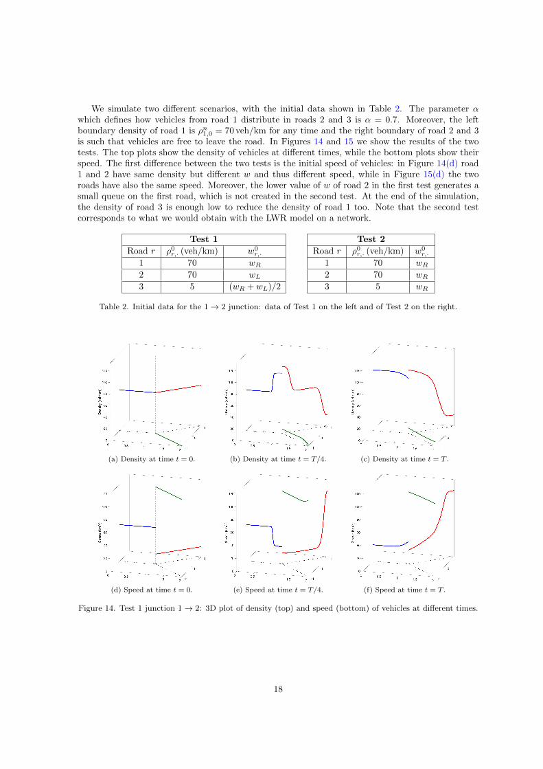
We simulate two different scenarios, with the initial data shown in Table 2. The parameter αwhich defines how vehicles from road 1 distribute in roads 2 and 3 is α = 0.7. Moreover, the leftboundary density of road 1 is ρn1,0 = 70 veh/km for any time and the right boundary of road 2 and 3is such that vehicles are free to leave the road. In Figures 14 and 15 we show the results of the twotests. The top plots show the density of vehicles at different times, while the bottom plots show theirspeed. The first difference between the two tests is the initial speed of vehicles: in Figure 14(d) road1 and 2 have same density but different w and thus different speed, while in Figure 15(d) the tworoads have also the same speed. Moreover, the lower value of w of road 2 in the first test generates asmall queue on the first road, which is not created in the second test. At the end of the simulation,the density of road 3 is enough low to reduce the density of road 1 too. Note that the second testcorresponds to what we would obtain with the LWR model on a network.

Test 1

Road r ρ0r,· (veh/km) w0r,·

1 70 wR2 70 wL3 5 (wR + wL)/2

Test 2


1 70 wR2 70 wR3 5 wR

Table 2. Initial data for the 1→ 2 junction: data of Test 1 on the left and of Test 2 on the right.

(a) Density at time t = 0. (b) Density at time t = T/4. (c) Density at time t = T .

(d) Speed at time t = 0. (e) Speed at time t = T/4. (f) Speed at time t = T .

Figure 14. Test 1 junction 1→ 2: 3D plot of density (top) and speed (bottom) of vehicles at different times.

18





Let us consider a junction with two incoming roads and one outgoing road, depicted in Figure 16. Thedensity of roads 1, 2 and 3 is computed with the 2CTM scheme on the cells outside the junction. Wesolve the Riemann problem at junction as described in Section 4.3 to obtain ρn1,Nx

= ρJ1 , ρn2,Nx= ρJ2

and ρn3,0 = ρJ3 , for n = 0, . . . , Nt.

1

2

3

J


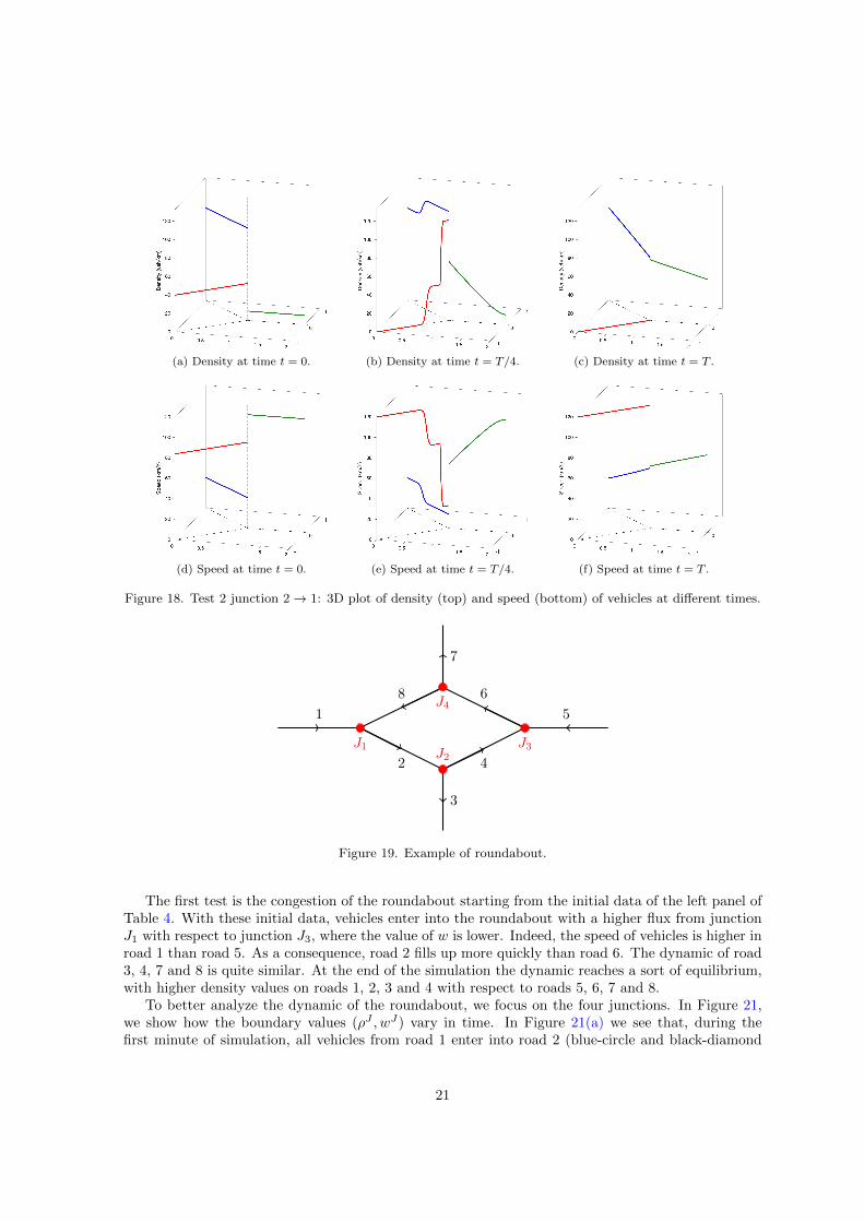
We simulate two different scenarios with the initial data taken as in Table 3. The parameter βwhich defines the priority rule is fixed as β = 0.6. In road 1 vehicles continues to enter with densityequal to 40 veh/km, no more vehicles enter into road 2 and the right boundary of road 3 is such thatvehicles are free to leave the road. Finally, we observe that in both the tests we allow vehicles to notrespect the priority rule. The test in Figure 17 shows that the lower value of w on road 2 is such thatvehicles slowly reach the junction, while road 1 fills up quickly. Once road 2 is empty, all vehicles ofroad 1 move to road 3. The test in Figure 18, instead, starts with all the roads with same w. In thiscase vehicles of both roads 1 and 2 reach quickly the junction and thus road 2 empties more quickly

19

with respect to test 1.

Test 1


1 40 wR2 30 wL3 10 (wR + wL)/2

Test 2


1 40 wR2 30 wR3 10 wR

Table 3. Initial data for the 2→ 1 junction: data of Test 1 on the left and of Test 2 on the right.




5.4 The case of a roundabout

Let us consider the roundabout depicted in Figure 19. We have four junctions: J1 and J3 of type2→ 1, involving roads 1 and 8 into road 2 and roads 4 and 5 into road 6, respectively, and J2 and J4of type 1→ 2, involving road 2 into roads 3 and 4 and road 6 into roads 7 and 8, respectively.

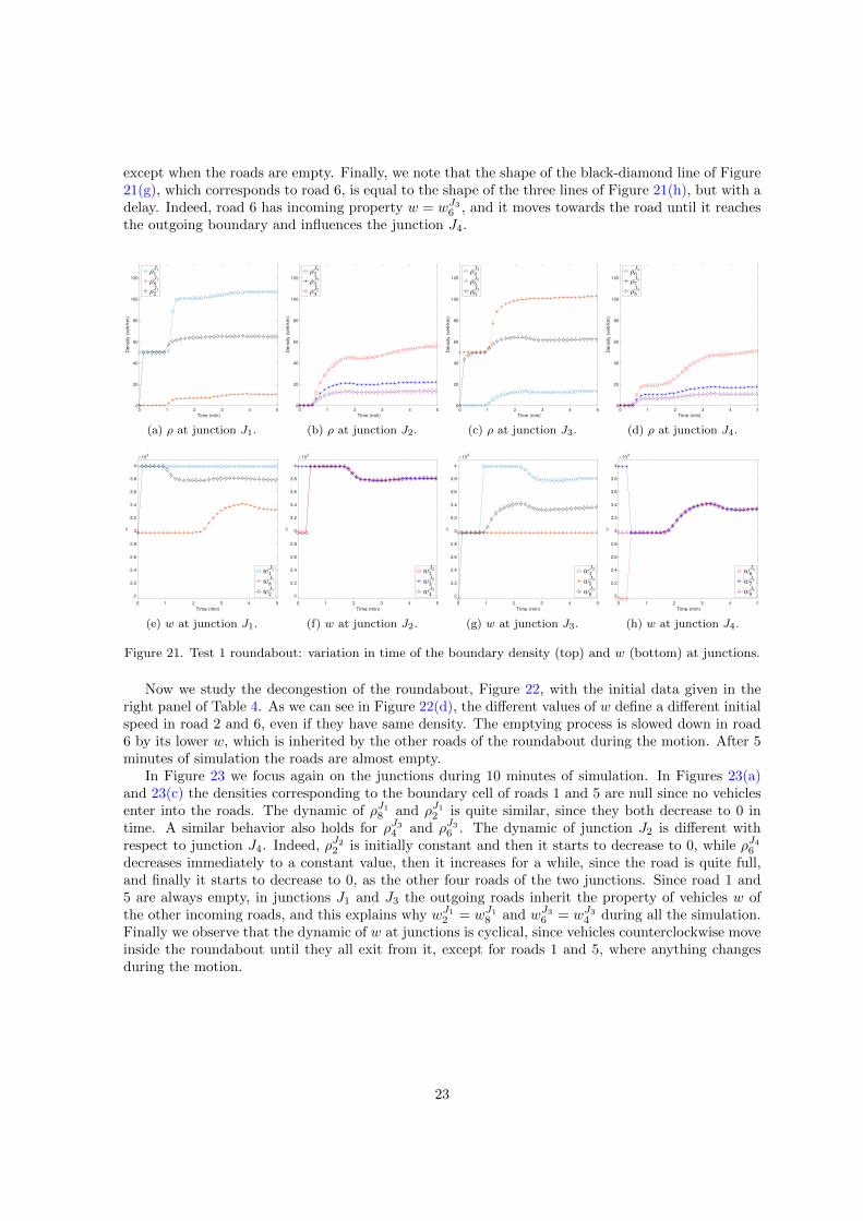
We treat junctions J1 and J3 as explained in Section 5.3 and junctions J2 and J4 as in Section5.2. Vehicles enter into roads 1 and 5 with constant rate and roads 3 and 7 are such that vehicles arefree to leave the network. The parameter α, which defines the distribution of vehicles for the 1 → 2junction is α = 0.6. In order to promote the motion on the roundabout, we define the parameterβ = 2/3 for the junction J1 and β = 1/3 for the junction J3. With this choices of β the dynamicfavors the flux of vehicles from road 8 more than road 1, and from road 4 more than road 5. We testtwo scenarios: the congestion and the decongestion of the roundabout.

20




1

2

3

4

5

6

7

8

J1J2

J3

J4

Figure 19. Example of roundabout.

The first test is the congestion of the roundabout starting from the initial data of the left panel ofTable 4. With these initial data, vehicles enter into the roundabout with a higher flux from junctionJ1 with respect to junction J3, where the value of w is lower. Indeed, the speed of vehicles is higher inroad 1 than road 5. As a consequence, road 2 fills up more quickly than road 6. The dynamic of road3, 4, 7 and 8 is quite similar. At the end of the simulation the dynamic reaches a sort of equilibrium,with higher density values on roads 1, 2, 3 and 4 with respect to roads 5, 6, 7 and 8.

To better analyze the dynamic of the roundabout, we focus on the four junctions. In Figure 21,we show how the boundary values (ρJ , wJ) vary in time. In Figure 21(a) we see that, during thefirst minute of simulation, all vehicles from road 1 enter into road 2 (blue-circle and black-diamond

21

Test 1: congestion of roundabout


1 50 wR

2 0 (wR + wL)/2

3 0 wR

4 0 (wR + wL)/2

5 50 (wR + wL)/2

6 0 wL

7 0 wR

8 0 (wR + wL)/2

Test 2: decongestion of roundabout


1 0 wR

2 70 (wR + wL)/2

3 0 wR

4 50 (wR + wL)/2

5 0 (wR + wL)/2

6 70 wL

7 50 wR

8 0 (wR + wL)/2

Table 4. Initial data for the roundabout: data of Test 1 on the left and of Test 2 on the right.

0

20

40

60

80

100

120


0

20

40

60

80

100

120


0

20

40

60

80

100

120


0

20

40

60

80

100

120


0

20

40

60

80

100

120


0

20

40

60

80

100

120


Figure 20. Test 1 roundabout: plot of density (top) and speed (bottom) of vehicles at different times withcolors scaling with respect to the corresponding color-bar.

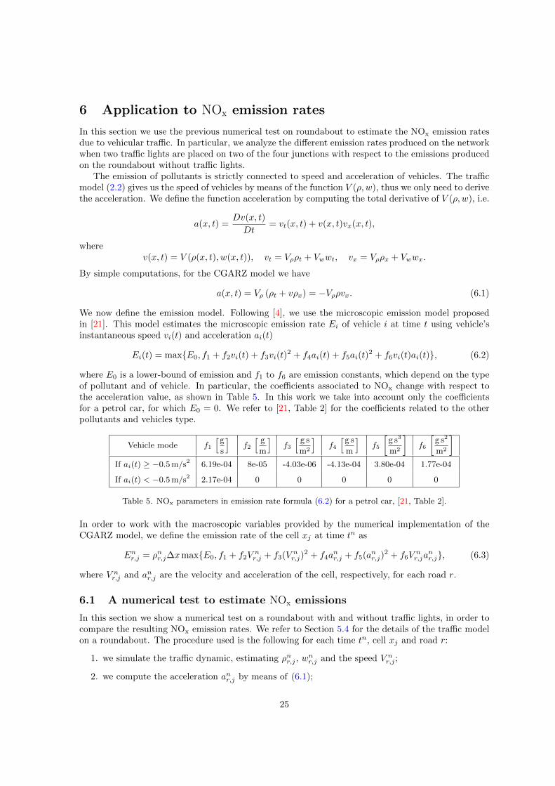
lines), since there are still no vehicles into road 8. Once vehicles of road 8 reach the right boundary,they have the priority with respect to road 1, for our choice of β, therefore we see the formation ofa queue at the end of road 1. The dynamic of the density at junction J3 represented in Figure 21(c)is quite similar, but it is slowed down by the lower value of w along the roads, see Figures 21(g) and21(e). Such analysis is applied also to junctions J2 and J3, since vehicles reach the right boundary ofroad 2 faster than road 6, as we can see from the red-circle lines of Figures 21(b) and 21(d), due tothe different values of w. Note that the parameter α is such that there are more vehicles which exitthe roundabout with respect to those which remain into it. Moreover, we observe that for the 1→ 2junctions (J2 and J4) we have same boundary w for all the roads by construction of the solution,

22

except when the roads are empty. Finally, we note that the shape of the black-diamond line of Figure21(g), which corresponds to road 6, is equal to the shape of the three lines of Figure 21(h), but with adelay. Indeed, road 6 has incoming property w = wJ36 , and it moves towards the road until it reachesthe outgoing boundary and influences the junction J4.

0 1 2 3 4 5

Time (min)

0

20

40

60

80

100

120

Density (

veh/k

m)

(a) ρ at junction J1.

0 1 2 3 4 5

Time (min)

0

20

40

60

80

100

120

Density (

veh/k

m)

(b) ρ at junction J2.

0 1 2 3 4 5

Time (min)

0

20

40

60

80

100

120

Density (

veh/k

m)

(c) ρ at junction J3.

0 1 2 3 4 5

Time (min)

0

20

40

60

80

100

120

Density (

veh/k

m)

(d) ρ at junction J4.

0 1 2 3 4 5

Time (min)

2

2.2

2.4

2.6

2.8

3

3.2

3.4

3.6

3.8

4

103

(e) w at junction J1.

0 1 2 3 4 5

Time (min)

2

2.2

2.4

2.6

2.8

3

3.2

3.4

3.6

3.8

4

103

(f) w at junction J2.

0 1 2 3 4 5

Time (min)

2

2.2

2.4

2.6

2.8

3

3.2

3.4

3.6

3.8

4

103

(g) w at junction J3.

0 1 2 3 4 5

Time (min)

2

2.2

2.4

2.6

2.8

3

3.2

3.4

3.6

3.8

4

103

(h) w at junction J4.

Figure 21. Test 1 roundabout: variation in time of the boundary density (top) and w (bottom) at junctions.

Now we study the decongestion of the roundabout, Figure 22, with the initial data given in theright panel of Table 4. As we can see in Figure 22(d), the different values of w define a different initialspeed in road 2 and 6, even if they have same density. The emptying process is slowed down in road6 by its lower w, which is inherited by the other roads of the roundabout during the motion. After 5minutes of simulation the roads are almost empty.

In Figure 23 we focus again on the junctions during 10 minutes of simulation. In Figures 23(a)and 23(c) the densities corresponding to the boundary cell of roads 1 and 5 are null since no vehiclesenter into the roads. The dynamic of ρJ18 and ρJ12 is quite similar, since they both decrease to 0 intime. A similar behavior also holds for ρJ34 and ρJ36 . The dynamic of junction J2 is different withrespect to junction J4. Indeed, ρJ22 is initially constant and then it starts to decrease to 0, while ρJ46decreases immediately to a constant value, then it increases for a while, since the road is quite full,and finally it starts to decrease to 0, as the other four roads of the two junctions. Since road 1 and5 are always empty, in junctions J1 and J3 the outgoing roads inherit the property of vehicles w ofthe other incoming roads, and this explains why wJ12 = wJ18 and wJ36 = wJ34 during all the simulation.Finally we observe that the dynamic of w at junctions is cyclical, since vehicles counterclockwise moveinside the roundabout until they all exit from it, except for roads 1 and 5, where anything changesduring the motion.

23

0

20

40

60

80

100

120


0

20

40

60

80

100

120


0

20

40

60

80

100

120


0

20

40

60

80

100

120


0

20

40

60

80

100

120


0

20

40

60

80

100

120


Figure 22. Test 2 roundabout: plot of density (top) and speed (bottom) of vehicles at different times withcolors scaling with respect to the corresponding color-bar.

0 1 2 3 4 5 6 7 8 9 10

Time (min)

0

20

40

60

80

100

120

Density (

veh/k

m)

(a) ρ at junction J1.

0 1 2 3 4 5 6 7 8 9 10

Time (min)

0

20

40

60

80

100

120

Density (

veh/k

m)

(b) ρ at junction J2.

0 1 2 3 4 5 6 7 8 9 10

Time (min)

0

20

40

60

80

100

120

Density (

veh/k

m)

(c) ρ at junction J3.

0 1 2 3 4 5 6 7 8 9 10

Time (min)

0

20

40

60

80

100

120

Density (

veh/k

m)

(d) ρ at junction J4.

0 1 2 3 4 5 6 7 8 9 10

Time (min)

2

2.2

2.4

2.6

2.8

3

3.2

3.4

3.6

3.8

4

103

(e) w at junction J1.

0 1 2 3 4 5 6 7 8 9 10

Time (min)

2

2.2

2.4

2.6

2.8

3

3.2

3.4

3.6

3.8

4

103

(f) w at junction J2.

0 1 2 3 4 5 6 7 8 9 10

Time (min)

2

2.2

2.4

2.6

2.8

3

3.2

3.4

3.6

3.8

4

103

(g) w at junction J3.

0 1 2 3 4 5 6 7 8 9 10

Time (min)

2

2.2

2.4

2.6

2.8

3

3.2

3.4

3.6

3.8

4

103

(h) w at junction J4.

Figure 23. Test 2 roundabout: variation in time of the boundary density (top) and w (bottom) at junctions.

24

6 Application to NOx emission rates

In this section we use the previous numerical test on roundabout to estimate the NOx emission ratesdue to vehicular traffic. In particular, we analyze the different emission rates produced on the networkwhen two traffic lights are placed on two of the four junctions with respect to the emissions producedon the roundabout without traffic lights.

The emission of pollutants is strictly connected to speed and acceleration of vehicles. The trafficmodel (2.2) gives us the speed of vehicles by means of the function V (ρ, w), thus we only need to derivethe acceleration. We define the function acceleration by computing the total derivative of V (ρ, w), i.e.

a(x, t) =Dv(x, t)

Dt= vt(x, t) + v(x, t)vx(x, t),

wherev(x, t) = V (ρ(x, t), w(x, t)), vt = Vρρt + Vwwt, vx = Vρρx + Vwwx.

By simple computations, for the CGARZ model we have

a(x, t) = Vρ (ρt + vρx) = −Vρρvx. (6.1)

We now define the emission model. Following [4], we use the microscopic emission model proposedin [21]. This model estimates the microscopic emission rate Ei of vehicle i at time t using vehicle’sinstantaneous speed vi(t) and acceleration ai(t)

Ei(t) = maxE0, f1 + f2vi(t) + f3vi(t)2 + f4ai(t) + f5ai(t)

2 + f6vi(t)ai(t), (6.2)

where E0 is a lower-bound of emission and f1 to f6 are emission constants, which depend on the typeof pollutant and of vehicle. In particular, the coefficients associated to NOx change with respect tothe acceleration value, as shown in Table 5. In this work we take into account only the coefficientsfor a petrol car, for which E0 = 0. We refer to [21, Table 2] for the coefficients related to the otherpollutants and vehicles type.

Vehicle mode f1[g

s

]f2[ g

m

]f3[ g s

m2

]f4[g s

m

]f5

[g s3

m2

]f6

[g s2

m2

]If ai(t) ≥ −0.5 m/s2 6.19e-04 8e-05 -4.03e-06 -4.13e-04 3.80e-04 1.77e-04

If ai(t) < −0.5 m/s2 2.17e-04 0 0 0 0 0

Table 5. NOx parameters in emission rate formula (6.2) for a petrol car, [21, Table 2].

In order to work with the macroscopic variables provided by the numerical implementation of theCGARZ model, we define the emission rate of the cell xj at time tn as

Enr,j = ρnr,j∆xmaxE0, f1 + f2Vnr,j + f3(V nr,j)

2 + f4anr,j + f5(anr,j)

2 + f6Vnr,ja

nr,j, (6.3)

where V nr,j and anr,j are the velocity and acceleration of the cell, respectively, for each road r.

6.1 A numerical test to estimate NOx emissions

In this section we show a numerical test on a roundabout with and without traffic lights, in order tocompare the resulting NOx emission rates. We refer to Section 5.4 for the details of the traffic modelon a roundabout. The procedure used is the following for each time tn, cell xj and road r:

1. we simulate the traffic dynamic, estimating ρnr,j , wnr,j and the speed V nr,j ;

2. we compute the acceleration anr,j by means of (6.1);

25

3. we estimate the emission rates Enr,j by means of (6.3).

The traffic simulation on the roundabout is computed with the initial data shown in Table 6 for atime of 120 min. We fix the length of each road of the roundabout equal to 3 km. We assume thatvehicles enter into road 1 and 5 with density equal to 100 veh/km and 90 veh/km respectively, andthat vehicles are free to leave roads 3 and 7. The parameter α of the 1→ 2 junctions is α = 0.4 andthe parameter β of the 2→ 1 junctions is β = 2/3 for junction J1 and β = 1/3 for junction J3.


1 100 wR

2 0 (wR + wL)/2

3 0 wL

4 0 (wR + wL)/2

5 90 (wR + wL)/2

6 0 wL

7 0 wL

8 0 (wR + wL)/2

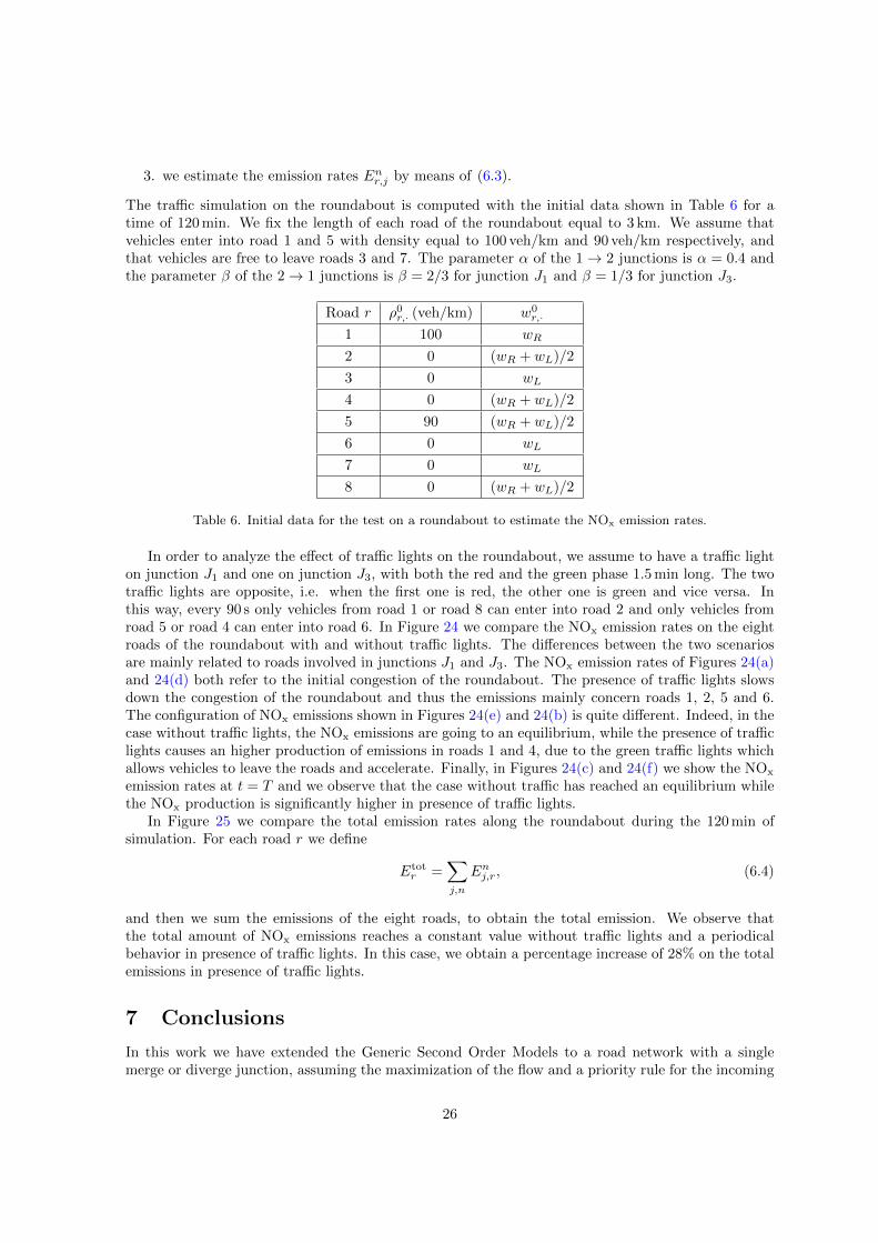
Table 6. Initial data for the test on a roundabout to estimate the NOx emission rates.

In order to analyze the effect of traffic lights on the roundabout, we assume to have a traffic lighton junction J1 and one on junction J3, with both the red and the green phase 1.5 min long. The twotraffic lights are opposite, i.e. when the first one is red, the other one is green and vice versa. Inthis way, every 90 s only vehicles from road 1 or road 8 can enter into road 2 and only vehicles fromroad 5 or road 4 can enter into road 6. In Figure 24 we compare the NOx emission rates on the eightroads of the roundabout with and without traffic lights. The differences between the two scenariosare mainly related to roads involved in junctions J1 and J3. The NOx emission rates of Figures 24(a)and 24(d) both refer to the initial congestion of the roundabout. The presence of traffic lights slowsdown the congestion of the roundabout and thus the emissions mainly concern roads 1, 2, 5 and 6.The configuration of NOx emissions shown in Figures 24(e) and 24(b) is quite different. Indeed, in thecase without traffic lights, the NOx emissions are going to an equilibrium, while the presence of trafficlights causes an higher production of emissions in roads 1 and 4, due to the green traffic lights whichallows vehicles to leave the roads and accelerate. Finally, in Figures 24(c) and 24(f) we show the NOx

emission rates at t = T and we observe that the case without traffic has reached an equilibrium whilethe NOx production is significantly higher in presence of traffic lights.

In Figure 25 we compare the total emission rates along the roundabout during the 120 min ofsimulation. For each road r we define

Etotr =

∑j,n

Enj,r, (6.4)

and then we sum the emissions of the eight roads, to obtain the total emission. We observe thatthe total amount of NOx emissions reaches a constant value without traffic lights and a periodicalbehavior in presence of traffic lights. In this case, we obtain a percentage increase of 28% on the totalemissions in presence of traffic lights.

7 Conclusions

In this work we have extended the Generic Second Order Models to a road network with a singlemerge or diverge junction, assuming the maximization of the flow and a priority rule for the incoming

26

0

5

10

15

20

25

30

35

(a) NOx emission rates withouttraffic lights at time t =7 min.

0

5

10

15

20

25

30

35

(b) NOx emission rates with-out traffic lights at time t =15.5 min.

0

5

10

15

20

25

30

35

(c) NOx emission rates withouttraffic lights at time t = T .

0

5

10

15

20

25

30

35

(d) NOx emission rates with traf-fic lights at time t = 7 min.

0

5

10

15

20

25

30

35

(e) NOx emission rates with traf-fic lights at time t = 15.5 min.

0

5

10

15

20

25

30

35

(f) NOx emission rates with traf-fic lights at time t = T .

Figure 24. NOx emission rates (g/km) on a roundabout without traffic lights (top) and with traffic lights inJ1 and J3 (bottom).

0 20 40 60 80 100 120

Time (min)

1.5

2

2.5

3

3.5

4

4.5

NO

x e

mis

sio

ns (

g/k

m)

103

No traffic light

Traffic light

Figure 25. Total NOx emission rates (g/km) along the whole roundabout.

roads at the merge junction. The numerical tests have shown the influence of the variable w on trafficdynamic, underlining the differences with respect to the LWR model on networks. Finally, we haveestimated the NOx emission rates produced on a roundabout, showing the increase of the emissions

27

in presence of traffic lights. The proposed procedure can be applied to any other pollutant associatedto vehicle traffic.

References

[1] C. Appert-Rolland, F. Chevoir, P. Gondret, S. Lassarre, J.-P. Lebacque, andM. Schreckenberg, eds., Traffic and granular flow ’07, Springer-Verlag, Berlin, 2009.

[2] R. Atkinson and W. P. Carter, Kinetics and mechanisms of the gas-phase reactions of ozonewith organic compounds under atmospheric conditions, Chem. Rev., 84 (1984), pp. 437–470.

[3] A. Aw and M. Rascle, Resurrection of “Second Order” Models of Traffic Flow, SIAM J. Appl.Math., 60 (2000), pp. 916–944.

[4] C. Balzotti, M. Briani, B. De Filippo, and B. Piccoli, Evaluation of NOx emissionsand ozone production due to vehicular traffic via second-order models, arXiv preprint arXiv:1912.05956, (2019).

[5] S. Blandin, D. Work, P. Goatin, B. Piccoli, and A. Bayen, A General Phase TransitionModel for Vehicular Traffic, SIAM J. Appl. Math., 71 (2011), pp. 107–127.

[6] R. M. Colombo, Hyperbolic Phase Transitions in Traffic Flow, SIAM J. Appl. Math., 63 (2003),pp. 708–721.

[7] C. F. Daganzo, Requiem for second-order fluid approximations of traffic flow, Transp. Res. B,29 (1995), pp. 277–286.

[8] M. L. Delle Monache, P. Goatin, and B. Piccoli, Priority-based Riemann solver for trafficflow on networks, Commun. Math. Sci., 16 (2018), pp. 185–211.

[9] S. Fan, M. Herty, and B. Seibold, Comparative model accuracy of a data-fitted generalizedAw-Rascle-Zhang model, Netw. Heterog. Media, 9 (2014), pp. 239–268.

[10] S. Fan and B. Seibold, Data-fitted first-order traffic models and their second-order generaliza-tions: Comparison by trajectory and sensor data, Transp. Res. Rec., 2391 (2013), pp. 32–43.

[11] S. Fan, Y. Sun, B. Piccoli, B. Seibold, and D. B. Work, A Collapsed Generalized Aw-Rascle-Zhang Model and its Model Accuracy, arXiv preprint arXiv:1702.03624, (2017).

[12] M. Garavello, K. Han, and B. Piccoli, Models for Vehicular Traffic on Networks, AmericanInstitute of Mathematical Sciences, 2016.

[13] M. Garavello and B. Piccoli, Traffic flow on a road network using the Aw-Rascle Model,Commun. Part. Diff. Eq., 31 (2006), pp. 243–275.

[14] M. Garavello and B. Piccoli, Traffic flow on networks, American Institute of MathematicalSciences, 2006.

[15] M. Garavello and B. Piccoli, Conservation laws on complex networks, Ann. Inst. H. PoincareAnal. Non Lineaire, 26 (2009), pp. 1925–1951.

[16] M. Herty, S. Moutari, and M. Rascle, Optimization criteria for modelling intersections ofvehicular traffic flow, Netw. Heterog. Media, 1 (2006), pp. 275–294.

[17] M. Herty and M. Rascle, Coupling conditions for a class of second-order models for trafficflow, SIAM J. Math. Anal., 38 (2006), pp. 595–616.

28

[18] H. Holden and N. H. Risebro, A mathematical model of traffic flow on a network of unidi-rectional roads, SIAM J. Math. Anal., 26 (1995), pp. 999–1017.

[19] J.-P. Lebacque, S. Mammar, and H. Haj-Salem, Generic second order traffic flow modelling,in Transportation and Traffic Theory, Elsevier, 2007, pp. 755–776.

[20] M. J. Lighthill and G. B. Whitham, On kinematic waves II. A theory of traffic flow on longcrowded roads, Proc. Roy. Soc. A, 229 (1955), pp. 317–345.

[21] L. I. Panis, S. Broekx, and R. Liu, Modelling instantaneous traffic emission and the influenceof traffic speed limits, Sci. Total Environ., 371 (2006), pp. 270–285.

[22] H. J. Payne, Models of freeway traffic and control, Proc. Simulation Council, 1 (1971), pp. 51–61.

[23] B. Piccoli, K. Han, T. L. Friesz, T. Yao, and J. Tang, Second-order models and trafficdata from mobile sensors, Transport. Res. C-Emer., 52 (2015), pp. 32 – 56.

[24] P. I. Richards, Shock Waves on the Highway, Operations Research, 4 (1956), pp. 42–51.

[25] G. B. Whitham, Linear and nonlinear waves, John Wiley and Sons, New York, 1974.

[26] H. M. Zhang, A non-equilibrium traffic model devoid of gas-like behavior, Transp. Res. B, 36(2002), pp. 275–290.

[27] K. Zhang and S. Batterman, Air pollution and health risks due to vehicle traffic, Sci. TotalEnviron., 450-451 (2013), pp. 307 – 316.

29

Estimate of emissions on road networks via Generic Second ...

Documents

Transcript of Estimate of emissions on road networks via Generic Second ...