Estadıstica IPractice for Chapter 3: Bivariate data analysis

Practice for Chapter 3: Bivariate data analysis

Contents

I Categorical dataI Contingency tableI Barchart

I Numerical data (Anscombe data set)I ScatterplotI Scatterplot matrixI Correlation matrix, covariance matrixI Simple linear regression

I ANOVA tableI Residual plot

Categorical data - creating data set

I Upload the following data set to R Commander

sex eyefemale blackmale blackmale bluemale greenmale greenfemale greenfemale blackmale greenfemale bluefemale blue

I Method 1: Type the table in the Notepad, save it and import to Rcmdr

I Method 2: Introduce directly in the Script Windowsex<-c(”female”,”male”,”male”,”male”,”male”,”female”,”female”,”male”,”female”,”female”)eye<-c(”black”,”black”,”blue”,”green”,”green”,”green”,”black”,”green”,”blue”,”blue”)DataSexEye<-data.frame(sex,eye)

Categorical data - contingency table

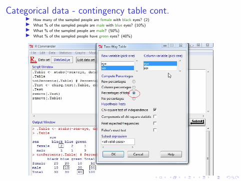
Categorical data - contingency table cont.I How many of the sampled people are female with black eyes? (2)I What % of the sampled people are male with blue eyes? (10%)I What % of the sampled people are male? (50%)I What % of the sampled people have green eyes? (40%)

Categorical data - barchartI Load the library lattice, then create barchart grouping the

data by sex

Categorical data - barchart cont.I Are there more females or males with blue eyes? (females)I What is the most common eye color among males? (green)

Freq

female

male

0.0 0.5 1.0 1.5 2.0 2.5 3.0

black blue

female

male

green

Numerical data - load anscombe data set from R library

Numerical data - scatterplot of y1 versus x1

Numerical data - scatterplot of y1 versus x1 cont.I Uncheck all but the Least-squares lineI Plotting characters 20 corresponds to bulletsI Increase the Point size to 2.5

Numerical data - scatterplot of y1 versus x1 cont.

4 6 8 10 12 14

45

67

89

1011

x1

y1

●

●

●

●

●

●

●

●

●

●

●

Numerical data - scatterplot matrix (only x1, x2, y1, y2)

Numerical data - scatterplot matrix (only x1, x2, y1, y2)cont.

I Check Least-squares line

Numerical data - scatterplot matrix (only x1, x2, y1, y2)cont.

x1

4 6 8 12

●

●

●

●

●

●

●

●

●

●

●

●

●

●

●

●

●

●

●

●

●

●

3 5 7 9

46

812

●

●

●

●

●

●

●

●

●

●

●

46

812

●

●

●

●

●

●

●

●

●

●

●

x2●

●

●

●

●

●

●

●

●

●

●

●

●

●

●

●

●

●

●

●

●

●

●

●

●

●●

●

●

●

●

●

●

●

●

●

●●

●

●

●

●

●

●

y1

46

810

●

●

●

●●

●

●

●

●

●

●

4 6 8 12

35

79 ●

●

●●●

●

●

●

●

●

●

●

●

●●●

●

●

●

●

●

●

4 6 8 10

●

●

● ●●

●

●

●

●

●

●

y2

Numerical data - correlation matrix

Numerical data - correlation matrix (only x1, x2, y1, y2)cont.

I Matrix is symmetrical with values on the diagonal = 1

I cor(x1, y1) = cor(y1, x1) = 0.8164205

Numerical data - covariance matrix (only x1, x2, y1, y2)

I Replace cor by cov in the last command in the Script Window

I cov(x1, y1) = 5.501

I Matrix is symmetrical with values on the diagonal = variances, eg,cov(y1, y1) = var(y1) = 4.127269

Simple linear regression - y1 versus x1

Simple linear regression - y1 versus x1 cont.

Simple linear regression - y1 versus x1 cont.

I Intercept estimate: a = 3.0001

I Slope estimate: b = 0.5001

I Residual standard deviation: sR =√∑n

i=1 r2i

n−2 = 1.237

I R-squared: R2 = 0.6665 ⇒ cor(x , y) =√

0.6665

Simple linear regression - residual plot (method 1)

Simple linear regression - residual plot (method 1) cont.I Residuals versus fitted (top left plot)

5 6 7 8 9 10

−2

−1

01

2

Fitted values

Res

idua

ls

●●

●

●

● ●

●

●

●

●

●

Residuals vs Fitted

3

9

10

●●

●

●

● ●

●

●

●

●

●

−1.5 −0.5 0.5 1.5

−1

01

2

Theoretical Quantiles

Sta

ndar

dize

d re

sidu

als

Normal Q−Q

3

9

10

5 6 7 8 9 10

0.0

0.4

0.8

1.2

Fitted values

Sta

ndar

dize

d re

sidu

als

●●

●

●

●

●

●

●

●●

●

Scale−Location39

10

0.00 0.10 0.20 0.30

−2

−1

01

2

Leverage

Sta

ndar

dize

d re

sidu

als

●●

●

●

● ●

●

●

●

●

●

Cook's distance1

0.5

0.5

1Residuals vs Leverage

3

9

10

lm(y1 ~ x1)

Simple linear regression - residual plot (method 2)I Append the fitted values, residuals, standardized residuals etc

to the existing data set

Simple linear regression - residual plot (method 2 cont.)I Append the fitted values, residuals, studentized residuals etc

to the existing data set

Simple linear regression - residual plot (method 2 cont.)I Now the data set has new columns on the right with y , r , etc

Simple linear regression - residual plot (method 2 cont.)I Use the scatterplot option in the Graphs menu to plot

residuals versus fitted

Simple linear regression - residual plot (method 2 cont.)

I Residuals versus fitted (cloud of points oscillates around thehorizontal axis y = 0)

I There is no pattern, no heteroscedasticity ⇒ regression model isappropriate

5 6 7 8 9 10

−2

−1

01

fitted.RegModel.1

resi

dual

s.R

egM

odel

.1

●●

●

●

●●

●

●

●

●

●

Simple linear regression - residual plot (method 2 cont.)

I Studentized Residuals ( risR

) versus x1 (cloud of points oscillates

around the horizontal axis y = 0)

I There is no pattern, no heteroscedasticity ⇒ regression model isappropriate

4 6 8 10 12 14

−2

−1

01

x1

rstu

dent

.Reg

Mod

el.1

●●

●

●

●●

●

●

●

●

●