Fearon, M. G., T. J. Brown, and G. M. Curcio, 2015: Establishing a national standard method for operational mixing height

determination. J. Operational Meteor., 3 (15), 172189, doi: http://dx.doi.org/10.15191/nwajom.2015.0315.

Corresponding author address: Matthew G. Fearon, 2215 Raggio Parkway, Reno, NV 89512

E-mail: matthew.fearon@dri.edu

172

Journal of Operational Meteorology

Article

Establishing a National Standard Method for Operational

Mixing Height Determination

MATTHEW G. FEARON and TIMOTHY J. BROWN

Desert Research Institute, Reno, Nevada

GARY M. CURCIO

IPA Fire Environment Specialist, LLC, La Grange, North Carolina

(Manuscript received 9 April 2015; review completed 2 September 2015)

ABSTRACT

Since the 1960s the Holzworth method has remained a primary tool for operational mixed-layer height

determination. The air volume through which ground-based pollutants vertically disperse defines the mixed

layer. The appeal of this method rests on the simple mechanics of making a forecast where knowledge of the

surface air temperature in concert with the background vertical structure is sufficient. The National Weather

Service routinely issues forecasts using this method for air-quality and wildland fire activities.

Methods of this type that are based principally on the static stability structure of the atmosphere and

exclude vapor content or dynamical processes (e.g., advection and wind shear) can misrepresent the mixing

height calculation. Systematic errors, such as the height being too low or high, can complicate wildland fire

activities (e.g., go/no-go burn decisions). Motivation for the present study emerges from this premise, and

thus examines the mixing height computed from four methods.

Mixing height methods employed in this study include Holzworth, Stull, bulk Richardson number, and

turbulent kinetic energy—where the latter two include dynamical processes. Mixing height also was derived

from satellite-based lidar data to provide an observed proxy and validation. Results from a method inter-

comparison show that turbulent kinetic energy is the most robust and well suited as a national standard

method for operational use—having both thermodynamic and dynamic processes incorporated. The bulk

Richardson number and Stull methods are other possibilities because their calculations are not model

dependent and heights are consistent with those from turbulent kinetic energy.

1. Introduction

Smoke from wildfire and prescribed burning in the

United States is important in terms of human health as

well as environmental and transportation safety (Moelt-

ner et al. 2013). Local dispersion is a major concern

for many wildland fire and air-quality agencies that

participate in wildfire and prescribed fire activities

[e.g., United States and State Forest Services, Bureau

of Land Management, National Weather Service Fore-

cast Offices (NWSFOs), and state and local air-quality

agencies]. Prediction of smoke dispersion indices (in-

cluding mixing height1, transport wind speed, and venti-

1 Mixing height and mixed-layer height are synonymous terms in

this paper. Mixing depth and mixed-layer depth also are synony-

mous and define the air volume between the ground and the

mixing height.

lation index) is a part of operational fire weather fore-

casts issued by NWSFOs. For the past several years,

the user community (e.g., local and state land manag-

ers, foresters, and personnel from the aforementioned

agencies) has expressed concern over the accuracy of

methods used to compute mixing height across

NWSFOs (National Wildfire Coordinating Group

2012–2015, personal communication), in particular the

widely used Holzworth method (Holzworth 1964,

1967). Local or regional discrepancies in the mixing

height calculation also arise when the Holzworth

method is used in a nonstandard fashion across

NWSFOs. Inconsistency in the method complicates

wildland fire go/no-go burn decisions and jeopardizes

wildfire impact assessments. The current study revisits

the Holzworth technique and three documented alter-

natives for mixing height determination—namely, the

Fearon et al. NWA Journal of Operational Meteorology 3 November 2015

ISSN 2325-6184, Vol. 3, No. 15 173

Stull, bulk Richardson number (RI), and turbulent

kinetic energy (TKE) methods—in order to determine

which method is the most robust and appropriate as a

national standard.

Seibert et al. (2000) defined the mixing height as

an upper boundary or lid in the atmosphere to which

ground-level pollutants vertically disperse. The devel-

opment of the mixed layer is a function of turbulence

that can arise from solar-induced thermal gradients

(the convection process), and/or mechanical stirring

from wind shear or advection. NWSFOs issue routine

fire weather forecasts that include mixing height based

primarily on the Holzworth method (see Table 1). This

procedure follows the adiabatic principle of parcel

theory and static stability where mixed-layer height is

traced to the altitude and intersection of the hypothet-

ical surface parcel with its environment, as shown in

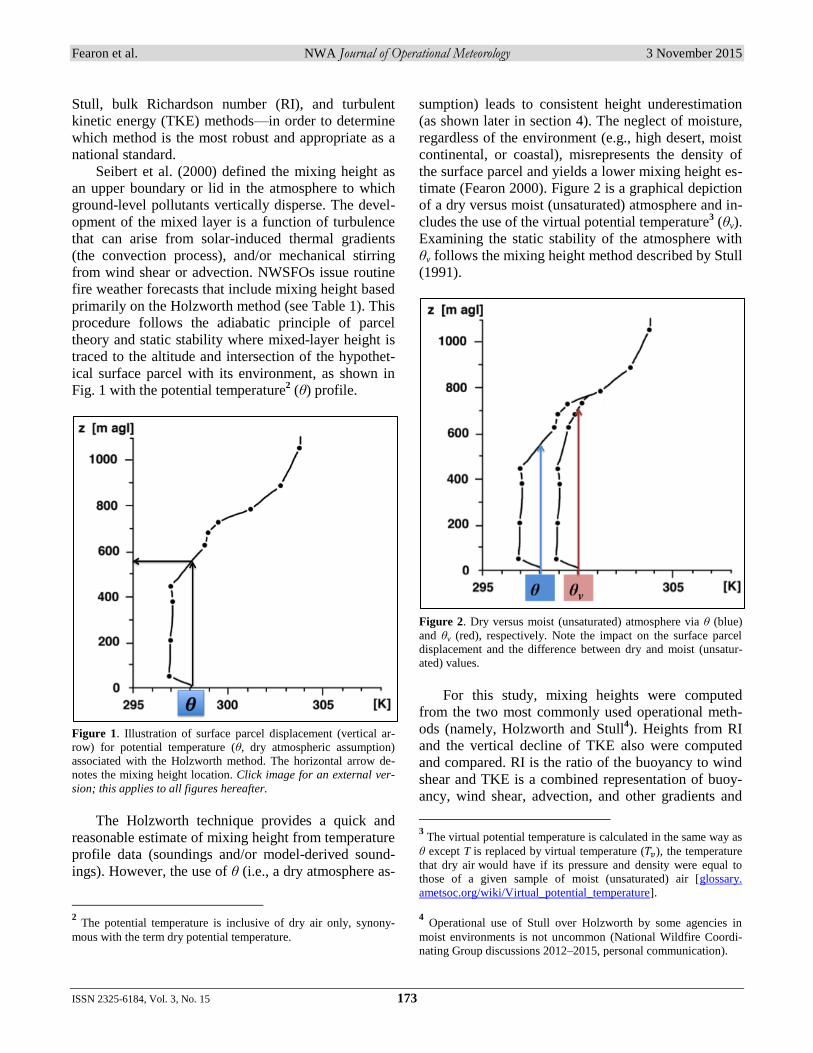
Fig. 1 with the potential temperature2 (θ) profile.

Figure 1. Illustration of surface parcel displacement (vertical ar-

row) for potential temperature (θ, dry atmospheric assumption)

associated with the Holzworth method. The horizontal arrow de-

notes the mixing height location. Click image for an external ver-

sion; this applies to all figures hereafter.

The Holzworth technique provides a quick and

reasonable estimate of mixing height from temperature

profile data (soundings and/or model-derived sound-

ings). However, the use of θ (i.e., a dry atmosphere as-

2 The potential temperature is inclusive of dry air only, synony-

mous with the term dry potential temperature.

sumption) leads to consistent height underestimation

(as shown later in section 4). The neglect of moisture,

regardless of the environment (e.g., high desert, moist

continental, or coastal), misrepresents the density of

the surface parcel and yields a lower mixing height es-

timate (Fearon 2000). Figure 2 is a graphical depiction

of a dry versus moist (unsaturated) atmosphere and in-

cludes the use of the virtual potential temperature3 (θv).

Examining the static stability of the atmosphere with

θv follows the mixing height method described by Stull

(1991).

Figure 2. Dry versus moist (unsaturated) atmosphere via θ (blue)

and θv (red), respectively. Note the impact on the surface parcel

displacement and the difference between dry and moist (unsatur-

ated) values.

For this study, mixing heights were computed

from the two most commonly used operational meth-

ods (namely, Holzworth and Stull4). Heights from RI

and the vertical decline of TKE also were computed

and compared. RI is the ratio of the buoyancy to wind

shear and TKE is a combined representation of buoy-

ancy, wind shear, advection, and other gradients and

3 The virtual potential temperature is calculated in the same way as

θ except T is replaced by virtual temperature (𝑇𝑣), the temperature

that dry air would have if its pressure and density were equal to

those of a given sample of moist (unsaturated) air [glossary.

ametsoc.org/wiki/Virtual_potential_temperature].

4 Operational use of Stull over Holzworth by some agencies in

moist environments is not uncommon (National Wildfire Coordi-

nating Group discussions 2012–2015, personal communication).

Fearon et al. NWA Journal of Operational Meteorology 3 November 2015

ISSN 2325-6184, Vol. 3, No. 15 174

Table 1. Survey of the mixing height methods used (as a first look) by two randomly chosen NWSFOs within each of the six regions.

Region Forecast Office Identifier Method Used Office Telephone

Pacific Guam GUM Not sure of method 671-472-0900

Pacific Hawaii HFO Not sure of method*a 808-973-5286

Western Missoula MSO Holzworthb 406-329-4840

Western Sacramento STO Holzworth 916-979-3051

Eastern Greenville GSP Holzworth 864-848-3859

Eastern State College CTP Holzworth 814-231-2408

Central Duluth DLH Holzworth 218-729-6697

Central Jackson JKL Holzworth 606-666-8000

Southern Birmingham BMX Holzworthc 205-664-3010

Southern Little Rock LZK Holzworth* 501-834-0308

Alaska Fairbanks AFG Holzworth 907-271-5088 / 907-458-3700

Alaska Anchorage AFC Holzworth 907-271-5088 / 907-266-5105

* Not satisfied with grid data provided. a High moisture content and inversions not reflected in grids.

b Currently evaluating Stull versus Holzworth methods.

c Current method under discussion.

perturbation terms that quantify the kinetic energy

throughout the atmospheric column. RI and TKE each

provide a combined measure of the static and dynamic

stability whereas Holzworth and Stull provide an esti-

mate of the static stability only. RI and TKE are well

documented in the literature (e.g., Vogelezang and

Holtslag 1996; Seibert et al. 1997; Zilitinkevich and

Baklanov 2002; Jeričević and Grisogono 2006; Lee et

al. 2008; Kiefer et al. 2015). Use of TKE for mixing

height determination is less common since computa-

tion requires finely resolved, evenly spaced data

(vertically and horizontally), such as from a numerical

model. Mixing heights from these four methods (Holz-

worth, Stull, RI, and TKE) also were compared to

those derived from satellite-based lidar where the latter

were chosen to represent observed data and provide an

independent measure. The spatial and temporal reso-

lution of the lidar data provided a large coincident

sample size against model grid points (discussed in

section 3).

Section 2 of this paper begins with a brief back-

ground into the origin of air-pollution control in the

United States and related research, including mention

of the classic mixed-layer model and boundary layer

concepts used in this study. Section 3 describes the

relevant data, the four mixing height methods of

interest—Holzworth, Stull, RI, and TKE—and the data

analysis methods used. Section 4 provides a discussion

of results from a mixing height method intercompari-

son. Examples of the vertical structure and spatial ex-

tent associated with mixing height discrepancies also

are presented. Section 5 is reserved for a summary of

results and recommendations from the authors on the

most robust approach for mixing height determination.

2. Background

The origin of comprehensive air pollution control

in the United States can be traced back to the mid-twentieth century. The National Air Pollution Act of

1955 and the Clean Air Act of 1963—and its subse-quent amendments in 1970 (McCarthy 2005)—repre-

sent two such pieces of regulatory legislation. Both were enacted in response to human health concerns

and the widespread increase of airborne contaminants from industrialization and mobile sources. Air-pollu-

tion research was one of the primary objectives out-lined in this legislation—in particular investigation of

urban emissions, dispersion, and transport in the

context of human health impacts. One of the central research themes to emerge during the 1960s was the

concept of monitoring and predicting the rate of at-mospheric dispersion and transport of airborne con-

taminants.

During the mid- to late-twentieth century numer-

ous studies were performed on atmospheric dispersion

in the low-level atmosphere, or the volume of air

designated as the mixed layer (e.g., Pasquill 1961;

Holzworth 1964; Turner 1964; Tennekes 1973; Yama-

da and Berman 1979; Stull 1991). Ball (1960) was

arguably the first to tackle the subject in the context of

the Archimedes Principle, where the density differen-

tial between the hypothetical surface parcel and its

Fearon et al. NWA Journal of Operational Meteorology 3 November 2015

ISSN 2325-6184, Vol. 3, No. 15 175

surrounding environment increases when solar heating

is introduced at the air–ground interface. In such cir-

cumstances, the static stability stratification of the air

column changes with unstable air developing at the

lower boundary and facilitating upward acceleration.

As the heated air mixes upward, eventually the density

differential in the air column becomes zero and the

upward acceleration vanishes. Yet, the momentum

gained on the upward journey carries air into the ad-

joining layer and simultaneously promotes downward

motion (or entrainment) of upper-level air. The turbu-

lent motion associated with the buoyancy and entrain-

ment leads to a stratified state where the temperature

decrease with height follows the adiabatic rate. Other

atmospheric constituents (e.g., wind, water vapor, and

pollution) that take part in the turbulent motion

become uniform in this mixed layer. This process be-

comes increasingly complex in the presence of over-

lying clouds such as non-precipitating cumulus (as

discussed by Lilly 1968 and Betts 1973).

Prognostic models of mixed-layer development

serve as another common method of height estimation.

Figure 3 illustrates the main sublayers of the mixed-

layer model at the time of maximum heating. These

include the shallow surface layer near the ground, the

deep turbulent (free convection) layer, and the entrain-

ment zone atop demarking the separation between the

boundary layer and the free atmosphere. This depic-

tion is representative of the mixed-layer (or jump)

model described by Tennekes (1973), Tennekes and

Driedonks (1981), Lewis (2007), and others, where the

important changes in the θ are a function of the varia-

tion in the buoyancy flux (𝑤′𝜃′; prime denotes pertur-

bation and overbar denotes mean) at the top and bot-

tom boundaries via the sharp increase and decrease,

respectively. The fundamental equation for this model

is given by:

𝜕𝜃

𝜕𝑡= [(𝑤′𝜃′)

𝑆− (𝑤′𝜃′)

𝐻] [

1

𝐻] (1)

where w is vertical velocity, H is the top of the mixed

layer, and S is the surface. Models of this type that

examine turbulent behavior over the entire depth of the

boundary layer are identified as nonlocal schemes.

Alternatively, attempts to quantify turbulent behavior

and static stability via localized gradients are identified

as local schemes. The latter methods often are incon-

sistent with observations, as most of the turbulent

energy is associated with the largest eddies, which

typically have influence over the full depth of the

Figure 3. Illustration adapted from Lewis (2007) of the classic

mixed-layer model at the mature stage. Note the sharp decrease in

θ and the upward acceleration arrow associated with the buoyancy

flux (𝑤′𝜃′ ) in the surface layer, the uniform profile in the free-

convection layer, and the increase or jump (σ) near the mixed-layer

top (H) associated with the entrainment layer.

Figure 4. Depiction of parcel displacements associated with the

Stull method via θv, including local versus nonlocal static stability

and flow type. Adapted from Stull (1991).

boundary layer (Stensrud 2007). Figure 4 illustrates

nonlocal versus local static stability classification for

an example sounding. Parcel displacements follow the

nonlocal definition where static stability and flow type

are evaluated over the entire atmospheric column. As-

sessment of the environmental profile and its vertical

variation over discrete segments follows the local defi-

nition.

As described by Stensrud (2007), Eq. 1 and the

concept of local versus nonlocal introduces the fun-

Fearon et al. NWA Journal of Operational Meteorology 3 November 2015

ISSN 2325-6184, Vol. 3, No. 15 176

damental problem associated with boundary layer

predictive schemes—namely, turbulence closure. As in

the previous mixed-layer model, instantaneous varia-

bles like θ and w are expressed in terms of their mean

and turbulent (perturbation) components (e.g., 𝜃 and

𝜃′ or 𝑤 and 𝑤′, respectively). And although the mean

quantity, ��/𝜕𝑡, is the desired parameter, it remains a

function of turbulent multiples or correlation terms

like the buoyancy flux (𝑤′𝜃′). The appearance of the

latter in the governing equation set introduces un-

known variables that require parameterization (or

approximation) where the principles of turbulence clo-

sure are utilized. A double correlation term like buoy-

ancy flux would follow first-order turbulence closure.

A triple correlation term (three turbulent multiples)

would follow second-order closure, and so on, where

the order follows the increase of turbulent multiples.

As with static stability assessment, turbulence closure

can be performed locally or non-locally. Nonlocal

closure relates unknown variables to known variables

at any number of other vertical grid points within the

column. Local closure relates known variables to un-

knowns at nearby vertical grid points. The principles

of closure gain in complexity with the addition of

terms and order of moments sought. Refer to Stull

(1988) for a more in-depth description of turbulence

closure.

Numerical schemes that characterize the planetary

boundary layer (PBL) utilize the principles of turbu-

lence closure to obtain a closed set of prognostic equa-

tions for temperature, moisture, and momentum. These

equations are then used to quantify TKE, a measure of

the intensity of turbulence. Descriptively, the tendency

for TKE to increase or decrease is given by:

Δ𝑇𝐾𝐸

Δ𝑡= 𝐴 + 𝑆ℎ + 𝐵 + 𝑇𝑟 − 𝜀 (2)

where A is the advection of TKE by the mean wind, Sh

is the shear generation, B is the buoyant production or

consumption, Tr is transport by turbulence motions

and pressure gradients, and 𝜀 is the viscous dissipation

rate. Each of the former terms contributes to the gener-

ation or consumption of TKE where the intensity de-

clines from the ground upward and dissipation typical-

ly identifies the top of the boundary layer.

Threshold values of TKE also are commonly used

to determine mixed-layer height. The ratio of buoy-

ancy to shear—the two most dominant terms in the

TKE equation—defines the RI (Stull 2000). According

to Richardson (1921), threshold values of RI can be

used to categorize flow type. Values 1 signify lami-

nar flow, while those <1 suggest turbulent flow. Rich-

ardson (1921) identified a critical value of 0.25 to

indicate when turbulent flow is certain. However,

since Richardson’s work, certain threshold values of

RI between 0.25 and 1.0 have been found to be

consistent with the TKE dissipation in the boundary

layer and the mixed-layer height. For example, a TKE

of 0.505 is a threshold used in the operational North

American Mesoscale (NAM) Forecast System (Janjić

2001; Lee et al. 2008).

3. Methods and data

For this study, afternoon mixing heights were

computed using the Holzworth, Stull, RI, and TKE for a two-year period (2009–2010) over the contiguous

United States. Source data for height calculations in-cluded hourly numerical model soundings and post-

processed profiles of aerosol extinction, as measured by satellite-based lidar. Mixing height methods, their

source data, and the analysis methods used are de-scribed in the following subsections.

a. Holzworth and Stull mixing height methods

Both the Holzworth and Stull methods rely on the

principles of static stability and parcel theory. The primary difference between the methods is the source

variable, θ versus θv, where the inclusion of moisture in the latter can yield a value greater than the former

by as much as 3°C (Fearon 2000). This difference in

the environmental profile with height, particularly near the surface, impacts the buoyancy assessment of the

surface parcel and the mixing height calculation (see Fig. 2). The mixing height from both methods is found

at the altitude at which the upward vertical displace-ment or the positive buoyancy of the surface parcel

terminates (also the parcel’s intersection with the environmental profile). Parcel displacement(s) for the

Holzworth and Stull methods are depicted in Figs. 1 and 4, respectively. Parcel displacements beyond that

of the surface parcel for the Stull method (Fig. 4) provide further detail on the static stability, particular-

ly the depth of instability and the associated flow type. As depicted, the depth of instability is not necessarily

consistent with the positive buoyancy of the surface parcel. In such cases, low-level stable air may become

well mixed in response to daytime heating or dynami-

cal forcing (see Figs. 4 and 5). Following either out-come, the surface buoyancy would become consistent

among the methods with differences again tied ex-clusively to the source variable (see Fig. 2).

Fearon et al. NWA Journal of Operational Meteorology 3 November 2015

ISSN 2325-6184, Vol. 3, No. 15 177

Figure 5. Same as Fig. 4 except the low-level inversion has now

mixed out. Local and nonlocal static stability now are equivalent.

b. TKE and RI mixing height methods

Profiles of TKE and its decline with height were

examined from model output (data described below)

where a threshold value of 0.1 J kg–1

is used to identify

the mixed-layer height (Fig. 6, left panel). As dis-

cussed in Holtslag and Moeng (1991), eddy diffusivity

calculations of heat and transport reveal that the value

of 0.1 corresponds consistently with boundary layer

inversion height. Lee et al. (2008) also described the

use of this threshold for TKE in relation to RI for plan-

etary boundary layer height determination within the

operational NAM.

RI represents the ratio of the buoyancy flux and

wind shear terms of the TKE equation. In bulk form,

the equation takes the form of:

𝑅𝐼 = (𝑔 𝜃𝑣

⁄ ) ∆𝜃𝑣 ∆𝑍

[(∆��)2+(∆��)2] (3)

where g is gravity, Z is height, U is the x component of

the wind, V is the y component of the wind, the nu-

merator represents the buoyancy (also the Brunt-

Väisälä frequency) as the vertical change in the mean

θv across the layer, and the denominator is the vertical

variation of the horizontal wind. In this study, a height

consistent with a threshold of 0.505 (unitless) from RI

identified the mixed-layer height following a profile

search from the ground upward (Janjić 2001; Lee et al.

Figure 6. Illustration of the TKE (left) and RI (right) mixing

height method mechanics. The thin gray vertical lines depict the

threshold limits of 0.1 J kg–1 (left) and 0.505 (right). The thin black

horizontal lines depict mixing height location in relation to the

threshold limits.

2008). An RI calculation that exceeds this value signi-

fies a decline in turbulence (Fig. 6, right panel). Note

that both TKE and RI include vapor content in their

respective calculations.

c. Rapid Update Cycle Version 2 (RUC2) analysis

The RUC2 is a hydrostatic model with 40 isen-

tropic-sigma hybrid model surfaces defining the verti-cal structure. Turbulent mixing, including the bound-

ary layer, is prescribed explicitly using the methods of Burk and Thompson (1989), a nonlocal scheme with

level-two closure (third-order moments are parameter-ized). Additional details on model physics can be

found in Benjamin et al. (2004). In this study, RUC2

model analysis grids for the period 2009–2010 were used to generate mixing heights. The hourly frequency

and horizontal grid spacing (13 km) provided colloca-tion opportunities for the satellite-based lidar data

(Fig. 7). Profiles of θ, θv, geopotential height, U, and V from RUC2 grid cells were extracted and used to

compute mixed-layer height for the Holzworth and Stull methods, along with RI. TKE profiles were also

available and used to determine a mixing height.

d. Lidar data

Aerosol retrievals from the National Aeronautics

and Space Administration (NASA) Cloud-Aerosol

Lidar and Infrared Pathfinder Satellite Observation

Fearon et al. NWA Journal of Operational Meteorology 3 November 2015

ISSN 2325-6184, Vol. 3, No. 15 178

Figure 7. Illustration of the RUC2 (blue) centroids in relation to

the CALIPSO lidar 5-km swath centers (green) over the contigu-

ous United States. Yellow dots depict radiosonde locations. Note

how lidar footprints and radiosonde locations often are not collo-

cated (per the zoomed in image at lower right).

(CALIPSO) system were used as an independent

measure of mixing height in this study. The CALIPSO

satellite follows a sun-synchronous polar orbit with a

16-day repeat cycle (Vaughan et al. 2004). It is part of

the Afternoon (A-Train) satellite constellation, which

currently includes Global Change Observation Mis-

sion-Water 1, Aqua, CALIPSO, CloudSat, and Orbit-

ing Carbon Observatory-2, where equatorial overpass

time for CALIPSO is 1330 local time (NASA 2015).

The Vertical Feature Mask (VFM, ver. 3.01) product

was chosen for its simplicity (Fig. 8), as it is a post-

processed version of the aerosol backscatter and pro-

vides aerosol depth classification for all or individual

constituents. Referencing Fig. 8, the horizontal foot-

print of the lidar beam is 5 km, within which are 15

individual profiles at a horizontal resolution of 333 m.

The vertical resolution of each profile is 30 m within

the first 8 km of the surface. The orange classification

defines the total aerosol depth and was chosen to

represent the mixed-layer depth5. For this definition,

the base of the aerosol layer had to be in contact or

within 60 m of the ground. The top of this aerosol

layer defined the mixing height location. If elevated

aerosol existed above this layer, and its horizontal

width was 2.5 km (half or more of the 5-km swath), a

60-m separation was allowed before a layer discon-

tinuity was assumed. If the horizontal width of the

elevated aerosol was <2.5 km, a discontinuous layer

was assumed. The choice of 60 m for aerosol layer

discontinuity detection represents twice the lidar verti-

5 The VFM algorithm is able to discriminate cloud and aerosol

when they coexist and therefore mixing height was determined

when clouds were present or not.

cal resolution and was found to be a representative

filter to remove unrealistic gaps in the vertical (caused

by minor beam attenuation). When employed, the local

variability of the aerosol profile remained consistent

with collocated numerical sounding structure.

The use of aerosol extinction—per the CALIPSO

layer products—as a surrogate of the mixed-layer

depth has been employed in other studies [namely,

Leventidou et al. (2013) and Wu et al. (2010)]. The

authors of the latter study found strong consistency

with aerosol extinction and VFM classification in the

context of mixing height determination. Note that

consistent post-processing algorithms for VFM aerosol

products influenced the two-year period chosen for

this study (2009–2010). Further, unusable retrievals

are not uncommon due to beam attenuation, and there-

fore, a subset of those depicted in Fig. 7 were found to

be worthy of mixing height determination. Additional

details regarding the CALIPSO system and data can

found in Vaughan et al. (2004).

e. Weather Research and Forecasting (WRF) data

In conjunction with mixing heights computed at

collocated points from RUC2 and lidar, an analysis

also was conducted for three geographic regions using

the mass core nonhydrostatic Advanced Research

WRF model (Skamarock et al. 2008). Three modeling

domains at 10-km grid spacing, each with a one-way

2-km nest, were used for three regional extents over

the Southeast, the northern Plains, and the western

United States (Fig. 9). These subregions were selected

in order capture a variety of airmass and terrain com-

plexities that affect mixed-layer variability across the

contiguous United States. The inner nest choice of 2-

km horizontal grid spacing followed the discussion

presented in Moeng and Wyngaard (1988) in conjunct-

tion with the finest resolution options possible given

local computing resources. The model configuration

remained consistent for all three domains with 47

levels in the vertical extending up to 15 km above

ground level (AGL), 18 vertical levels below 1.5 km

AGL, with the lowest model level set at 10 m AGL.

The model physics included (1) momentum and heat

fluxes at the surface that use an Eta surface layer

scheme following Monin-Obukhov similarity theory

(Janjić 2001), (2) turbulence parameterization follow-

ing the Mellor-Yamada-Nakanishi-Niino (MYNN;

Nakanishi and Niino 2004) scheme, (3) convective

processes following the Kain-Fritsch cumulus scheme

for 10-km horizontal grid size, (4) cloud microphysical

Fearon et al. NWA Journal of Operational Meteorology 3 November 2015

ISSN 2325-6184, Vol. 3, No. 15 179

Figure 8. CALIPSO VFM browse image for a 5-km wide lidar footprint (south to north trajectory) and

the associated feature classifications, where orange illustrates total aerosol within the column (left

image). Footprint data are stored as sub-blocks comprising 15 individual profiles where the vertical and

horizontal resolution of each profile is 60 m 333 m, respectively, within the first 8 km (right image). In

this example, mixing height would be approximately 2.5 km AGL.

Figure 9. WRF nested domains for the Southeast (top), northern Plains (bottom left), and western

United States (bottom right). The outer (inner) domain for each location was 10-km (2-km) grid spacing

with each domain center denoted in yellow as 1 (2), respectively.

Fearon et al. NWA Journal of Operational Meteorology 3 November 2015

ISSN 2325-6184, Vol. 3, No. 15 180

processes following explicit bulk representation of

microphysics (Thompson et al. 2004, 2006), (5) radi-

ative processes parameterized using the Rapid Radia-

tive Transfer Model for longwave radiation (Mlawer et

al. 1997) and Dudhia's shortwave scheme (Dudhia

1989), and (6) the land-surface processes following the

Noah land surface model that provides the surface

sensible, latent heat, and upward longwave and

shortwave fluxes to the atmospheric model (Chen and

Dudhia 2001; Ek et al. 2003). Note that the MYNN

turbulence parameterization for PBL was a critical

choice for this study because the buoyancy and shear

contributions from TKE are partitioned as separate

output variables in WRF.

f. Data analysis methods

The analysis of afternoon mixing heights deter-

mined from RUC2, lidar, and WRF is presented in

section 4. Values from the four methods were first

examined in terms of their overall distributions from

RUC2 versus lidar. A mixing height difference of 500

m was chosen to represent a significant discrepancy6.

Such discrepancies were evaluated further using WRF

model output for the three geographic regions (Fig. 9).

The goal of the latter was to address two questions.

First, does finer resolution in the horizontal (and verti-

cal) explain height discrepancies among the methods

because eddy motions and flux terms represented by

the TKE equation would be better resolved? Second,

what is the physical meaning of the mixing height

produced by each method, in terms of the vertical

structure and across space?

Methods employed to evaluate vertical structure

included profile analysis of buoyancy, shear, and θv.

Colored maps of TKE contribution, partitioned by

term for each 2-km domain, were developed to evalu-

ate spatial variance. Mixing height differences >500 m

at a particular grid point assumed the following color

assignment: 1) if buoyancy was present alone, points

were colored red; 2) if shear was present alone, points

were colored green; 3) if both terms were operative,

points were colored blue; and 4) if neither term was

operative, points were colored black, signifying that

advection and/or topographic effects were active for an

elevation >250 m. TKE contribution for buoyancy and

shear was examined through perturbation values. Such

6 This value derives from Holzworth (1964) where the minimum

mean annual mixing height range over the contiguous United

States was found to be 200–800 m. The 500-m value represents the

midpoint.

values were computed for each model level using the

value at each grid point minus the average over the

entire domain. These deviations were then integrated

through the column for levels within the determined

mixed-layer volume.

4. Discussion of results

a. Mixing heights from RUC2 and lidar

Figure 10 illustrates the distributions of mixing

heights computed for all four methods using RUC2

data (light blue) versus those estimated from lidar

(red). Overall, a low bias is prevalent across all meth-

od distributions with values from RI and Stull reveal-

ing a slightly larger variance. Examination of the me-

dian differences (departure from lidar) reveals devia-

tions (rounded to the nearest integer) of 100, 200, 200,

and 650 m for RI, Stull, TKE, and Holzworth, respec-

tively. In the case of Holzworth, 450 m of the median

deviation (the departure from Stull) corresponds di-

rectly to the exclusion of vapor content. As described

in section 3a, the fundamental difference between the

Holzworth and Stull mixing height calculation rests on

the source variable, θ versus θv, respectively. There-

fore, if Holzworth heights were recomputed using θv

instead of θ, values would become synonymous with

those from Stull.

Figure 10. Boxplot diagrams of mixing heights derived from lidar

(red) and RUC2 data for TKE, Stull, RI, and Holzworth (light blue,

respectively). The black horizontal dashed line highlights the me-

dian height for lidar in relation to the four methods. The colloca-

tion sample size is 2151.

Figure 11 is similar to Fig. 10, except scatter com-

parisons of height (each method versus lidar) are

shown. One-to-one distribution trends are similar a-

mong TKE, Stull, and RI, and reaffirm the small

median departures in Fig. 10, although variance and

patterns of low bias are not consistent. Note the linear

collection of points along the x axis depicted in Stull

and Holzworth versus lidar. For either method, a near

Fearon et al. NWA Journal of Operational Meteorology 3 November 2015

ISSN 2325-6184, Vol. 3, No. 15 181

Figure 11. Four-panel scatter diagrams depicting mixing heights

computed from RUC2 for each method versus lidar-derived height.

The yellow highlighted points are discussed in Fig 12. The colloca-

tion sample size is 2151.

zero height is indicative of a subtle low-level inversion

prematurely capping the surface parcel buoyancy.

Because this pattern is missing from the TKE and RI

distributions, mixed-layer growth on these particular

days was likely a result of dynamical forcing (e.g.,

shear) and that static-stability assessment alone was

not sufficient. This situation can persist or be tempo-

rary depending on the meteorological environment

(e.g., thermal capping or shear increasing, respective-

ly). In persistent cases, inversion strength becomes

important and is reflected by low mixing heights from

all the methods. However, in the majority of cases,

subtle near-surface inversions were properly resolved

when vapor and/or wind shear are accounted for in the

mixing height calculation. Figure 12 (related to the

yellow points in Fig. 11) exemplifies such a scenario

for a grid cell just west of Savannah, Georgia, at 1900

UTC 1 May 2009 (1500 local time) where a subtle,

near-surface inversion in θ led to an underestimated

mixing height from the Holzworth method (i.e., blue

line in the amplified part of Fig. 12). The inclusion of

moisture properly resolves the θ profile via the Stull

method (red line), although the true depth of the mixed

layer is function of static and dynamic stability per the

values of TKE and RI (purple and green lines, respec-

tively). The inclusion of both static and dynamic sta-

bility in the RI and TKE methods is reflected in their

distributions against lidar (Fig. 11) where, in general,

scatter is more symmetric about the one-to-one line.

For the RI distribution, variance is larger overall and

more evenly spread. The one-to-one relationship of

Figure 12. The vertical profiles of the yellow highlighted points in

Fig. 11 at a grid cell just west of Savannah, Georgia, at 1900 UTC

1 May 2009. The profiles are shown over a 3-km depth for the

TKE, RI, and combined Holzworth/Stull (blue/red lines; θ/θv)

methods from left to right. Thin vertical black lines designate

thresholds for the surface parcel temperature, and horizontal lines

define the mixing heights. For the combined Holzworth/Stull pan-

el, mixing heights (horizontal lines) are the bottom/top, respective-

ly. The subtle near-surface inversion for the Holzworth method is

shown in the blow-up panel (right-hand side) and marked by black

dashed lines/arrows.

TKE versus lidar reveals less variance throughout,

even though a low bias exists.

To quantify the distribution similarities, mixing

heights from Stull, TKE, and RI (Holzworth excluded)

were examined spatially. First, daily values from these

three methods are presented as a combined mean,

where the deviation from lidar (absolute value differ-

ence) at coincident locations is shown in Fig. 13. Red

(black) dots represent differences 500 m (<500 m).

The percentage of red and black dots is 35% and 65%

of the total, respectively. Figure 14 duplicates Fig. 13,

except now the red (black) dots represent height devi-

ations across the three methods only, with lidar height

removed. Now, the percentage of red and black dots is

15% and 85%, respectively. These two calculations

reveal that large height differences (across methods)

occur 15% of time, and when the method results are

combined, mean values differ from lidar 20% of the

time (i.e., 35% minus 15%). Height discrepancies per

method likely are produced because of dynamical pro-

cesses, where method inclusion (or not) and the level

of representation of the dynamics terms impact the

mixing height. The 20% departure from lidar height

also may suggest mixing height overestimation from

lidar where the vertical distribution of aerosol is not

always fully representative, particularly the upper

bound.

Fearon et al. NWA Journal of Operational Meteorology 3 November 2015

ISSN 2325-6184, Vol. 3, No. 15 182

Figure 13. Map of absolute mixing height differences, derived as the combined mean height (for

Stull, TKE, and RI from the RUC2) minus the coincident lidar height. Red (black) dots indicate

values 500 m (<500 m), respectively.

Figure 14. Map of absolute mixing height difference across methods (for TKE, RI, and Stull) from

RUC2 (lidar excluded). Red (black) dots indicate differences 500 m (<500 m). The three yellow

dots identify locations examined as case studies for the Southeast, northern Plains, and the western

United States (from east to west); refer to Table 2.

Lidar height being an overestimate is conjecture,

but could have merit under the following circum-

stances. For instance, mixing height estimation from

lidar is defined by the aerosol termination or the first

sizeable discontinuity with height, per the VFM

product described in section 3d. What if the aerosol

top was not sharply delineated, but instead diffused

across the mixed-layer boundary as a result of the

entrainment process (e.g., Fig. 3)? In the entrainment

zone, internal fluid properties of heat, moisture, and

momentum from the mixed-layer air below are vigor-

ously stirred with the air above (from the free atmos-

phere). Therefore, the delineation of aerosol particles

may be a function of the entrainment intensity and the

derived mixing height may be accurate to within a few

hundred meters. Of course, the quantity and type of

Fearon et al. NWA Journal of Operational Meteorology 3 November 2015

ISSN 2325-6184, Vol. 3, No. 15 183

aerosol present has implications on this theory. Aer-

osol type (e.g., dust, smoke, continental versus marine)

was examined for several locations, and type discrimi-

nation did not impact the altitude of the aerosol top. In

addition, the confidence value provided for feature

classification (e.g., aerosol versus cloud particle or

other) was examined. Restriction of pixels associated

with lower confidence did not impact results.

b. Mixing height differences—evaluation of vertical

structure using WRF

For this exercise, data for each of the three yellow

dots in Fig. 14 identified a significant mixing height

difference or discrepancy among the TKE, Stull, and

RI methods. Regional classification names (Southeast,

northern Plains, and western United States) were used

to reference each point. Table 2 shows the breakdown

of mixing heights for each location for both the RUC2

and WRF model output. Lidar mixing heights also are

given. Holzworth heights were excluded from this

analysis simply because the method mechanics are

identical to the surface parcel displacement used for

Stull where the use of vapor content is the only out-

standing difference in the calculation.

Table 2. RUC2/WRF mixing heights from the TKE, Stull, and RI

methods, as well as lidar (CALIPSO), for the three case study lo-

cations (yellow dots in Fig. 14).

Mixing Height (m)

Method Southeast Northern

Plains

Western

United States

TKE 1444/2184 3026/2519 1415/3439

Stull 2022/2089 1102/2661 2652/2905

RI 1931/1659 837/1419 2194/2616

Lidar 1965 2995 1846

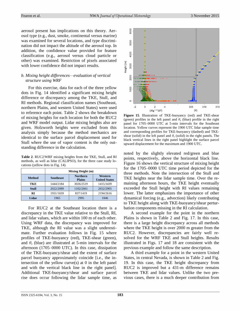
For RUC2 at the Southeast location there is a

discrepancy in the TKE value relative to the Stull, RI,

and lidar values, which are within 100 m of each other.

Using WRF data, the discrepancy was improved for

TKE, although the RI value was a slight underesti-

mate. Further evaluation follows in Fig. 15 where

profiles of TKE-buoyancy (red), TKE-shear (green),

and θv (blue) are illustrated at 5-min intervals for the

afternoon (1705–0000 UTC). In this case, dissipation

of the TKE-buoyancy/shear and the extent of surface

parcel buoyancy approximately coincide [i.e., the in-

tersection of the yellow curve(s) at 0 in the left panel

and with the vertical black line in the right panel].

Additional TKE-buoyancy/shear and surface parcel

rise does occur following the lidar sample time, as

Figure 15. Illustration of TKE-buoyancy (red) and TKE-shear

(green) profiles in the left panel and θv (blue) profile in the right

panel for 1705–0000 UTC at 5-min intervals for the Southeast

location. Yellow curves represent the 1900 UTC lidar sample time

and corresponding profiles for TKE-buoyancy (dashed) and TKE-

shear (solid) in the left panel and θv (solid) in the right panels. The

black vertical lines in the right panel highlight the surface parcel

upward displacement for the maximum and 1900 UTC.

noted by the slightly elevated red/green and blue

points, respectively, above the horizontal black line.

Figure 16 shows the vertical structure of mixing height

for the 1705–0000 UTC time period depicted for the

three methods. Note the intersection of the Stull and

TKE heights near the lidar sample time. Over the re-

maining afternoon hours, the TKE height eventually

exceeded the Stull height with RI values remaining

lower. The latter emphasizes the importance of other

dynamical forcing (e.g., advection) likely contributing

to TKE height along with TKE-buoyancy/shear pertur-

bation components missing in the RI calculation.

A second example for the point in the northern

Plains is shown in Table 2 and Fig. 17. In this case,

there is a large height discrepancy across all methods

where the TKE height is over 2000 m greater from the

RUC2. However, discrepancies are fairly well re-

solved for the WRF TKE and Stull heights. Results

illustrated in Figs. 17 and 18 are consistent with the

previous example and follow the same description.

A third example for a point in the western United

States, in central Nevada, is shown in Table 2 and Fig.

19. In this case, the TKE height discrepancy from

RUC2 is improved but a 431-m difference remains

between TKE and lidar values. Unlike the two pre-

vious cases, there is a much deeper contribution from

Fearon et al. NWA Journal of Operational Meteorology 3 November 2015

ISSN 2325-6184, Vol. 3, No. 15 184

Figure 16. Time-height profile of mixing heights for TKE (red),

Stull (blue), and RI (green) from the WRF for the Southeast loca-

tion. Temporal resolution is every 5 min from 1705–0000 UTC.

Vertical and horizontal black lines highlight the 1900 UTC lidar

sample time (consistent with the yellow curves in Fig. 15) and

mixing height location, respectively.

Figure 17. Same as Fig. 15 except for the northern Plains where

the yellow curves identify the 2000 UTC lidar sample time.

Figure 18. Same as Fig. 16 except for the northern Plains where

the black vertical line corresponds to the 2000 UTC lidar sample

time.

Figure 19. Same as Fig. 15 except for the western United States

the where yellow curves identify the 2100 UTC lidar sample time.

Figure 20. Same as Fig. 16 except for the western United States

where the black vertical line corresponds to the 2100 UTC lidar

sample time.

TKE-shear (Fig. 19, solid yellow curve in left panel).

Greater TKE-shear likely corresponds to the presence

of complex terrain, and with a heterogeneous moun-

tain-valley landscape like central Nevada, daytime

upslope flow accelerations in response to surface heat-

ing are common. Like the two previous examples,

mixing heights from the three methods follow a sim-

ilar trend during the afternoon (Fig. 20).

Mixing height determination with higher resolu-

tion numerical soundings better resolves the method

discrepancies. Values from TKE and Stull appear to

collapse on each other for a period before an elevated

separation develops during the mid- to late-afternoon

where TKE calculates a higher value. The question

then becomes, is a consistently higher value from TKE

a result of perturbation terms; is it a function of addi-

Fearon et al. NWA Journal of Operational Meteorology 3 November 2015

ISSN 2325-6184, Vol. 3, No. 15 185

tional terms in the TKE equation (e.g., advection); or,

is TKE and its chosen threshold simply an overesti-

mate? In the next subsection, a spatial analysis of

TKE-buoyancy/shear perturbations, including terrain

aspects, sheds more light on this discussion. RI is not

included in the remaining analysis as it truly is a proxy

for TKE with a more conservative threshold.

c. Mixing height differences—evaluation of spatial

variance using WRF

Figure 21 (left panel) illustrates the mixing height

differences between the methods (TKE minus Stull)

over the Southeast WRF 2-km grid-spacing domain.

Differences appear subtle owing to the fine resolution,

but are present nonetheless. The center panel of Fig.

21 portrays the differences in terms of the perturba-

tions using the grid cell coloring approach (section 3f).

Higher TKE values owing to buoyancy are present in

isolated locations. Green (shear) and blue (buoyancy

and shear) cells are noteworthy where the low-level

flow field (largely anticyclonic, Fig. 21, right panel)

has slight speed/directional changes imbedded. Contri-

butions also are evident near terrain rises and coast-

lines where the upstream flow is orthogonal. The most

interesting differences are located on the leeward slope

of the southern Appalachians over western North Car-

olina, where Stull values exceed those from TKE. This

pattern is consistent with leeward airmass descent and

warming in the surface layer at the lower elevation.

This conjecture is supported by the northwesterly flow

upstream, which is orthogonal to higher terrain on

approach, where the air rises (descends) and cools

(warms) on the windward (leeward) slope. In this sit-

uation, a strong superadiabatic surface layer ensues at

lower elevation southeast of the higher terrain and the

low-level parcel buoyancy is maximized. This discrep-

ancy between Stull and TKE values was found to be

temporary (~2 h), as the air column mixed vertically,

with TKE eventually portraying an elevated value

similar to the profile examples. Overall, higher TKE

values are well explained via perturbation components

of buoyancy and shear, suggesting that elevated values

are a byproduct.

Figure 22 portrays a second example for a 2-km

grid-spacing WRF domain over the northern Plains.

Here, larger TKE values dominate again with a few

isolated Stull values over southern North Dakota (left

panel). As before, the larger Stull values were found to

be temporary. In this situation, the low-level flow is

confluent overall with cyclonic and anticyclonic re-

gimes, northwest and southeast, respectively (right

panel), amplifying the westerly advection (right pan-

el). There are some impressive terrain rises in western

South Dakota and eastern Wyoming, not excluding the

moderate high points in west-central Minnesota. These

locations reveal larger TKE values (left and center

panel) orchestrated by terrain rises and orthogonal ad-

vection upstream. Elsewhere, perturbations in buoy-

ancy and shear independently or together promote

larger TKE values.

Figure 23 represents a third spatial example over

the western United States highlighting central Nevada.

Complex terrain dominates the landscape with pre-

dominately weak southerly flow (right panel). There

are several north–south mountain ranges across

Nevada, and mixing height differences are found along

these features (left panel). In this example, higher Stull

values are more evident, which are largely explainable

owing to superadiabatic surface layers. As before, such

differences were found to be temporary and surpassed

by TKE. Shear-based differences are scattered across

central–eastern Nevada in the presence of light/

variable flow (center and right panel). Elsewhere, dif-

ferences are explained by buoyancy alone or together

with shear.

Overall, larger mixing height differences (TKE

versus Stull) are well explained by the spatial pertur-

bation analysis. Grid cells of perturbation types were

collocated with large height differences (>500 m).

Buoyancy perturbations also were found in grid cells

where height differences were <500 m; however, the

magnitude of the perturbation was reduced. The same

can be said for shear- and terrain-induced perturba-

tions, including advective-based perturbations, unless

the flow was highly amplified, curved, or orthogonal

to topographic irregularities. These findings in combi-

nation with TKE’s robust account of all turbulent

motion sources—particularly those associated with

dynamical processes—explain why height differences

exist between these two methods.

5. Discussion of results

In this study, mixing heights from four methods

(TKE, Stull, RI, and Holzworth) were examined.

Results from each method were compared with one

another and against lidar-derived mixing height esti-

mates. A series of diagnostic analyses also was con-

ducted over space and time for point locations and

spatial extent where topographic features and airmass

exposure are highly variable. Table 3 provides a break-

Fearon et al. NWA Journal of Operational Meteorology 3 November 2015

ISSN 2325-6184, Vol. 3, No. 15 186

Figure 21. Maps of TKE-Stull height differences (m, left), spatial perturbations (center), and terrain (m) overlain by the 850-mb wind (kt)

for the Southeast 2-km grid-spacing WRF domain. Perturbation occurrence is represented by color for buoyancy (red, B), shear (green, S),

buoyancy and shear (blue, B+S), and advection and/or terrain inducement (black, AT).

Figure 22. Same as Fig. 21 except for the northern Plains domain.

Figure 23. Same as Fig. 21 except for the western United States domain with the 700-mb level representing the flow field (right).

down of advantages and disadvantages for each meth-

od.

The TKE method stands out as the most robust in

terms of inclusiveness of both thermodynamic and

dynamic processes in the boundary layer. Lee et al.

(2008) discussed how TKE may be an overestimate of

the true mixed-layer depth owing to the entrainment of

TKE by horizontal and vertical advection and diffu-

Fearon et al. NWA Journal of Operational Meteorology 3 November 2015

ISSN 2325-6184, Vol. 3, No. 15 187

Table 3. Summary of mixing height method advantages and disadvantages.

Method Advantages Disadvantages

TKE Incorporates all turbulent sources/sinks (buoyancy,

shear, advection, terrain influence, and others) Fine-resolution model dependency (e.g., 5-km grid spacing)

RI

Not model dependent

Buoyancy and shear

Surrogate for TKE dominant terms

Mean profile state exclusively, turbulent perturbations excluded

Excludes advection

Stull

Not model dependent

Diagnostic method for entire profile

Quick interpretation

Mean profile state exclusively, turbulent perturbations excluded

Buoyancy only

Holzworth Not model dependent

Quick interpretation

Mean profile state exclusively, turbulent perturbations excluded

Dry atmosphere

Surface parcel buoyancy only

sion processes near the PBL top using the 12-km

NAM model. However, these processes facilitate mix-ing through the entire column and precise discrimi-

nation near the PBL top may require reexamination of a chosen TKE threshold (e.g., 0.1 J kg

–1). Case exam-

ples shown in this paper demonstrate that large mixing height differences occur when dynamical processes

influence the overall calculation (e.g., 15% of the time, Fig. 14 and section 4a). Mixing height sensitivity to

shear and buoyancy perturbations, including advec-tion, as shown in section 4d, also demonstrates the

importance of dynamical processes and that a numeri-cal formulation of TKE is required to capture such

processes. The Stull method proves to be a reasonable ap-

proach to mixed-layer height estimation. However, the method relies on parcel theory and displacement ther-

modynamics only. The RI approach is an attempt to

remedy dynamical exclusion, but advective processes and perturbation components are not included. The use

of the RI flux number—inclusive of perturbation com-ponents—would be a more complete treatment. How-

ever, use of the latter, like TKE, would require a nu-merical model to calculate perturbation terms.

As mentioned earlier, the use of the Holzworth method is discouraged overall. Its use in arid locales

when low humidities are present has merit; however, the viewpoint of the unsaturated atmosphere via θv

accommodates both dry and moist situations. There-fore, use of θ for this application is unnecessary.

Based on the findings of this study, the authors recommend the TKE method for operational mixing

height prediction. And although this method requires a fine-resolution numerical model of at least 5-km hor-

izontal grid spacing7, this approach yields a derived

7 The 5-km assertion (corresponding to fine resolution) is based on

the lidar swath resolution used in this study, the discussion in

Moeng and Wyngaard (1988), and the current NAM Nest horizon-

tal grid spacing of 4 km over the continental United States.

mixing height inclusive of both thermodynamic and

dynamic processes where the mixing budget in the vertical and horizontal is quantified using a prognostic

equation as part of a numerical PBL scheme. An alter-native to TKE-based mixing height is the diagnostic

variable “PBL height,” which is available as part of operational NAM model output. The RI and Stull

methods are both sound diagnostic approaches with minor shortcomings (see Table 3), but represent viable

alternatives when numerical model output with TKE is unavailable.

Acknowledgments. The authors thank Joseph J.

Charney, Scott L. Goodrick, Michael L. Kaplan, John M.

Lewis, Brian E. Potter, and John Tomko for their con-

structive comments and editorial assistance. We are grateful

to Erin C. Gleason for her assistance with graphics, and ac-

knowledge NWA JOM Editors Jon Zeitler and Michael C.

Coniglio, and the three reviewers, who provided comments

that improved the manuscript. The authors also acknowl-

edge the cooperation and collaboration of the U.S. Depart-

ment of Energy as part of the Atmospheric Radiation Meas-

urement Climate Research Facility who provided the RUC2

analysis grids used in this study. Partial support for this

project was provided by the USDA Forest Service Cali-

fornia and Nevada Smoke and Air Committee Agreement

Number 09-CS-11052012-266 and the USDA Forest Ser-

vice National Interagency Fire Center Agreement Number

11-CS-11130206-075.

REFERENCES

Ball, F. K., 1960: Control of inversion height by surface

heating. Quart. J. Roy. Meteor. Soc., 86, 483–494,

CrossRef.

Benjamin, S. G., G. A. Grell, J. M. Brown, T. G. Smirnova,

and R. Bleck, 2004: Mesoscale weather prediction with

the RUC hybrid isentropic–terrain-following coordinate

model. Mon. Wea. Rev., 132, 473–494, CrossRef.

Fearon et al. NWA Journal of Operational Meteorology 3 November 2015

ISSN 2325-6184, Vol. 3, No. 15 188

Betts, A. K., 1973: Non-precipitating cumulus convection

and its parameterization. Quart. J. Roy. Meteor. Soc.,

99, 178–196, CrossRef.

Burk, S. D., and W. T. Thompson, 1989: A vertically nested

regional numerical weather prediction model with

second-order closure physics. Mon. Wea. Rev., 117,

2305–2324, CrossRef.

Chen, F., and J. Dudhia, 2001: Coupling an advanced land

surface–hydrology model with the Penn State–NCAR

MM5 modeling system. Part I: Model implementation

and sensitivity. Mon. Wea. Rev., 129, 569–585,

CrossRef.

Dudhia, J., 1989: Numerical study of convection observed

during the Winter Monsoon Experiment using a meso-

scale two-dimensional model. J. Atmos. Sci., 46, 3077–

3107, CrossRef.

Ek, M. B., K. E. Mitchell, Y. Lin, E. Rogers, P. Grunmann,

V. Koren, G. Gayno, and J. D. Tarpley, 2003:

Implementation of Noah land surface model advances

in the National Centers for Environmental Prediction

operational mesoscale Eta model. J. Geophys. Res.,

108, 8851, CrossRef.

Fearon, M. G., 2000: The use of nonlocal static stability to

determine mixing height from NCEP Eta model output

over the Western U.S. M.S. thesis, Dept. of

Atmospheric Sciences, University of Nevada, 161 pp.

[Available online at www.cefa.dri.edu/Publications/

mfearon_msthesis.pdf.]

Holtslag, A. A. M., and C.-H. Moeng, 1991: Eddy diffusivi-

ty and countergradient transport in the convective

atmospheric boundary layer. J. Atmos. Sci., 48, 1690–

1698, CrossRef.

Holzworth, G. C., 1964: Estimates of mean maximum

mixing depths in the contiguous United States. Mon.

Wea. Rev., 92, 235–242, CrossRef.

____, 1967: Mixing depths, wind speeds and air pollution

potential for selected locations in the United States. J.

Appl. Meteor., 6, 1039–1044, CrossRef.

Janjić, Z. I., 2001: Nonsingular implementation of the

Mellor-Yamada Level 2.5 scheme in the NCEP Meso

model. NCEP Office Note No. 437, 61 pp. [Available

online at www.lib.ncep.noaa.gov/ncepofficenotes/files/

on437.pdf.]

Jeričević, A., and B. Grisogono, 2006: The critical bulk

Richardson number in urban areas: Verification and

application in a numerical weather prediction model.

Tellus A, 58, 19–27, CrossRef.

Kiefer, M. T., W. E. Heilman, S. Zhong, J. J. Charney, and

X. Bian, 2015: Mean and turbulent flow downstream of

a low-intensity fire: Influence of canopy and back-

ground atmospheric conditions. J. Appl. Meteor.

Climatol., 54, 42–57, CrossRef.

Lee, P., and Coauthors, 2008: Impact of consistent boundary

layer mixing approaches between NAM and CMAQ.

Environ. Fluid Mech., 9, 23–42, CrossRef.

Leventidou, E., P. Zanis, D. Balis, E. Giannakaki, I.

Pytharoulis, and V. Amiridis, 2013: Factors affecting

the comparisons of planetary boundary layer height

retrievals from CALIPSO, ECMWF and radiosondes

over Thessaloniki, Greece. Atmos. Environ., 74, 360–

366, CrossRef.

Lewis, J. M., 2007: Use of a mixed-layer model to

investigate problems in operational prediction of return

flow. Mon. Wea. Rev., 135, 2610–2628, CrossRef.

Lilly, D. K., 1968: Models of cloud-topped mixed layers

under a strong inversion. Quart. J. Roy. Meteor. Soc.,

94, 292–309, CrossRef.

McCarthy, J. E., 2005: Clean Air Act: A summary of the act

and its major requirements. CRS Report for Congress,

Order Code RL30853, 25 pp. [Available online at

fpc.state.gov/documents/organization/47810.pdf.]

Mlawer, E. J., S. J. Taubman, P. D. Brown, M. J. Iacono,

and S. A. Clough, 1997: Radiative transfer for

inhomogeneous atmospheres: RRTM, a validated

correlated-k model for the longwave. J. Geophys. Res.,

102, 16663–16682, CrossRef.

Moeltner, K., M.-K. Kim, E. Zhu, and W. Yang, 2013:

Wildfire smoke and health impacts: A closer look at

fire attributes and their marginal effects. J. Environ.

Econ. Manag., 66, 476–496, CrossRef.

Moeng, C.-H. and J. C. Wyngaard, 1988: Spectral analysis

of large-eddy simulations of the convective boundary

layer. J. Atmos. Sci., 45, 3573–3587, CrossRef.

Nakanishi, M., and H. Niino, 2004: An improved Mellor–

Yamada Level-3 model with condensation physics: Its

design and verification. Bound-Lay Meteorol., 112, 1–

31, CrossRef.

NASA, cited 2015: The Cloud-Aerosol Lidar and Infrared

Pathfinder Satellite Observation (CALIPSO). [Avail-

able online at www-calipso.larc.nasa.gov.]

Pasquill, F., 1961: The estimation of the dispersion of

windborne material. Meteor. Mag., 90, 33–49.

Richardson, L. F., 1921: Some measurements of atmos-

pheric turbulence. Philos. Trans. R. Soc., A, 221, 1–28,

CrossRef.

Seibert, P., F. Beyrich, S.-E. Gryning, S. Joffre, A.

Rasmussen, and P. Tercier, 1997: Mixing height

determination for dispersion modelling. European

Commission, COST Action 710, Report of Working

Group 2, 121 pp. [Available online at imp.boku.ac.at/

envmet/finalreport_cost710-2.pdf.]

____, ____, ____, ____, ____, and ____, 2000: Review and

intercomparison of operational methods for the

determination of the mixing height. Atmos. Environ.,

34, 1001–1027, CrossRef.

Skamarock, W. C., and Coauthors, 2008: A Description of

the Advanced Research WRF Version 3. NCAR Tech.

Note NCAR/TN–475+STR, 125 pp. [Available online

at www2.mmm.ucar.edu/wrf/users/docs/arw_v3.pdf.]

Fearon et al. NWA Journal of Operational Meteorology 3 November 2015

ISSN 2325-6184, Vol. 3, No. 15 189

Stensrud, D. J., 2007: Parameterization Schemes: Keys to

Understanding Numerical Weather Prediction Models.

Cambridge University Press, 480 pp.

Stull, R. B., 1988: An Introduction to Boundary Layer

Meteorology. Kluwer Academic Publishers, 666 pp.

____, 1991: Static stability—an update. Bull. Am. Meteor.

Soc., 72, 1521–1529, CrossRef.

____, 2000: Meteorology for Scientists and Engineers.

Brooks/Cole, 502 pp.

Tennekes, H., 1973: A model for the dynamics of the

inversion above a convective boundary layer. J. Atmos.

Sci., 30, 558–567, CrossRef.

____, and A. G. M. Driedonks, 1981: Basic entrainment

equations for the atmospheric boundary layer. Bound-

Lay Meteorol., 20, 515–531, CrossRef.

Thompson, G, R. M. Rasmussen, and K. Manning, 2004:

Explicit forecasts of winter precipitation using an

improved bulk microphysics scheme. Part I:

Description of sensitivity analysis. Mon. Wea. Rev.,

132, 519–542, CrossRef.

____, P. R. Field, W. D. Hall, R. M. Rasmussen, 2006: A

new bulk microphysics parameterization for WRF and

MM5. Seventh Weather and Research Forecasting

Workshop, NCAR, Boulder, CO.

Turner, D. B., 1964: A diffusion model for an urban area. J.

Appl. Meteor., 3, 83–91, CrossRef.

Vaughan, M. A., S. A. Young, D. M. Winker, K. A. Powell,

A. H. Omar, Z. Liu, Y. Hu, and C. A. Hostetler, 2004:

Fully automated analysis of space-based lidar data: an

overview of the CALIPSO retrieval algorithms and data

products. Proc. SPIE 5575, Laser Radar Techniques for

Atmospheric Sensing, 16, CrossRef.

Vogelezang, D. H. P., and A. A. M. Holtslag, 1996:

Evaluation and model impacts of alternative boundary-

layer height formulations. Bound-Lay Meteorol., 81,

245–269, CrossRef.

Wu, Y., C.-M. Gan, L. Cordero, B. Gross, F. Moshary, and

S. Ahmed, 2010: PBL-height derivation from the

CALIOP/CALIPSO and comparing with the radiosonde

and ground-based lidar measurements. Proc. SPIE

7832, Lidar Technologies, Techniques, and Measure-

ments for Atmospheric Remote Sensing VI, 78320C,

CrossRef.

Yamada, T., and S. Berman, 1979: A critical evaluation of a

simple mixed-layer model with penetrative convection.

J. Appl. Meteor., 18, 781–786, CrossRef.

Zilitinkevich, S., and A. Baklanov, 2002: Calculation of the

height of the stable boundary layer in practical appli-

cations. Bound-Lay Meteorol., 105, 389–409, CrossRef.