Essays on the Economics of Retirement and …discovery.ucl.ac.uk/1473149/1/FinalVersion.pdfEssays on...
224
Essays on the Economics of Retirement and Pensions Gemma Charlotte Tetlow A dissertation submitted in partial fulfilment of the requirements for the degree of Doctor of Philosophy of University College London. Department of Economics University College London 7th September, 2015
Transcript of Essays on the Economics of Retirement and …discovery.ucl.ac.uk/1473149/1/FinalVersion.pdfEssays on...
Essays on the Economics of Retirement andPensions
Gemma Charlotte Tetlow
A dissertation submitted in partial fulfilment
of the requirements for the degree of
Doctor of Philosophy
of
University College London.
Department of Economics
University College London
7th September, 2015

2

3
I, Gemma Charlotte Tetlow, confirm that the work presented in this thesis is my own. No
part of this thesis has been presented before to any university or college for submission
as part of a higher degree. Chapter 2 was undertaken as joint work with Jonathan Cribb
and Carl Emmerson. Chapter 3 draws on joint work with James Banks (University of
Manchester) and Carl Emmerson. Chapters 4 and 5 are sole authored. Where information
has been derived from other sources, I confirm that this has been indicated in the thesis.
Signature:
Date: 7th September, 2015


Abstract
The papers in this thesis use household survey data to examine financial decisions made at
the end of working life and in early retirement. Chapters 2 and 3 focus on the timing of
retirement. Chapters 4 and 5 examine the importance of longevity expectations for financial
decision-making.
Chapter 2 examines the impact of an increase in the early retirement age for women in
the UK. Women’s employment rates at age 60 increased by 7.3 percentage points when the
early retirement age increased to 61 and employment rates of male partners increased by 4.2
percentage points. The results suggest these effects are more likely explained by the policy
change having a signalling effect rather than being due to credit constraints or changes in
financial incentives.
Chapter 3 examines how responsive retirement decisions are to dynamic financial in-
centives. On average both men and women respond significantly to these financial incent-
ives. However, responses to these financial incentives alone are not sufficient to explain the
‘spikes’ in retirement that are observed in practice.
Chapter 4 shows that, overall, individuals understand how their chances of survival
compare to other people of their age and sex (e.g. those who engage in poor health be-
haviours expect lower chances of surviving than healthier people) and individuals’ expect-
ations are predictive of their subsequent mortality. However, I also show that individuals
perceive a ‘flatter’ survival curve than standard life tables would suggest. Two simple mod-
els of life cycle behaviour demonstrate that this misperception of longevity could explain
some apparently ‘puzzling’ behaviour seen in practice.
Chapter 5 examines the importance of private information about longevity in the mar-
ket for annuities. This chapter shows that there is adverse selection. However, it remains
an open question what the welfare loss is, particularly since individuals misperceive their
chances of survival on average.


Acknowledgements
I am very grateful to James Banks and Richard Blundell for their guidance and supervi-
sion. I am particularly grateful to Richard for helping me through the final stages. I am
also grateful to my colleagues at the Institute for Fiscal Studies – in particular to Rowena
Crawford, Jonathan Cribb, Richard Disney, Carl Emmerson and Cormac O’Dea – for their
support, help, advice and general good humour. Without these people, this thesis would not
have been possible.
I am also indebted to my family for their support and encouragement. Particular thanks
go to my mum for proof-reading much of my draft thesis – and for accepting in some cases
that ‘that is just how economists write’.
This thesis was made possible by financial support from the ESRC-funded Centre for
the Microeconomic Analysis of Public Policy (CPP) at the Institute for Fiscal Studies (grant
number RES-544-28-5001). Additional financial support for the work in Chapter 2 was also
gratefully received from the Nuffield Foundation (grant number OPD/40207) and the IFS
Retirement Saving Consortium.
The Labour Force Survey, Living Costs and Food Survey, and Family Resources Sur-
vey data (used in Chapters 2 and 3) are Crown Copyright material and are used with the
permission of the Controller of HMSO and the Queen’s Printer for Scotland. The English
Longitudinal Study of Ageing (used in Chapters 3-5) is funded by the National Institute
on Aging and a consortium of UK government departments. The copyright is held jointly
by the Institute for Fiscal Studies, the National Centre for Social Research and University
College London. The data were supplied by the UK Data Service. Responsibility for in-
terpretation of the data and the views expressed here, as well as for any errors, is mine
alone.


Contents
1 Introduction . . . . . . . . . . . . . . . . . . . . . . . . . . . . . . . . . . . . . . 19
1.1 Pensions and the timing of retirement . . . . . . . . . . . . . . . . . . . . . . 19
1.2 Expectations of survival and economic behaviour . . . . . . . . . . . . . . . 21
2 Increasing the female state pension age in the UK: Effects on labour supply of
older women and their husbands . . . . . . . . . . . . . . . . . . . . . . . . . . . 25
2.1 Introduction . . . . . . . . . . . . . . . . . . . . . . . . . . . . . . . . . . . 25
2.2 Related literature . . . . . . . . . . . . . . . . . . . . . . . . . . . . . . . . 29
2.3 Background and data . . . . . . . . . . . . . . . . . . . . . . . . . . . . . . 31
2.3.1 Institutional details . . . . . . . . . . . . . . . . . . . . . . . . . . . . 31
2.3.2 Data . . . . . . . . . . . . . . . . . . . . . . . . . . . . . . . . . . . . 35
2.4 Empirical methodology . . . . . . . . . . . . . . . . . . . . . . . . . . . . . 39
2.5 Results . . . . . . . . . . . . . . . . . . . . . . . . . . . . . . . . . . . . . . 41
2.5.1 Effect on women’s employment rates . . . . . . . . . . . . . . . . . . 41
2.5.2 Effect on different subgroups . . . . . . . . . . . . . . . . . . . . . . . 44
2.5.3 Effect on broader measures of economic status . . . . . . . . . . . . . 47
2.5.4 Effect on the economic status of men . . . . . . . . . . . . . . . . . . 49
2.5.5 Effect on the public finances . . . . . . . . . . . . . . . . . . . . . . . 52
2.6 Conclusions . . . . . . . . . . . . . . . . . . . . . . . . . . . . . . . . . . . 53
Appendices . . . . . . . . . . . . . . . . . . . . . . . . . . . . . . . . . . . . . . . 56
2.A Additional tables and figures . . . . . . . . . . . . . . . . . . . . . . . . . . 56
2.B Effect on employment before age 60 . . . . . . . . . . . . . . . . . . . . . . 62
3 Can dynamic financial incentives explain older workers’ labour supply? . . . . . . 65
3.1 Introduction . . . . . . . . . . . . . . . . . . . . . . . . . . . . . . . . . . . 65
3.2 Institutional details . . . . . . . . . . . . . . . . . . . . . . . . . . . . . . . 70
3.2.1 State pensions . . . . . . . . . . . . . . . . . . . . . . . . . . . . . . 70

10 Contents
3.2.2 Private pensions . . . . . . . . . . . . . . . . . . . . . . . . . . . . . 72
3.2.3 Taxes and benefits . . . . . . . . . . . . . . . . . . . . . . . . . . . . 75
3.3 Methodology . . . . . . . . . . . . . . . . . . . . . . . . . . . . . . . . . . 78
3.3.1 The option value model . . . . . . . . . . . . . . . . . . . . . . . . . 78
3.3.2 Empirical implementation . . . . . . . . . . . . . . . . . . . . . . . . 79
3.4 Data and descriptives . . . . . . . . . . . . . . . . . . . . . . . . . . . . . . 83
3.4.1 Sample selection . . . . . . . . . . . . . . . . . . . . . . . . . . . . . 83
3.4.2 Measuring education . . . . . . . . . . . . . . . . . . . . . . . . . . . 86
3.4.3 Measuring health . . . . . . . . . . . . . . . . . . . . . . . . . . . . . 86
3.4.4 Survival probabilities . . . . . . . . . . . . . . . . . . . . . . . . . . . 90
3.4.5 Calculating private pension entitlements . . . . . . . . . . . . . . . . 91
3.4.6 Calculating state pension entitlements . . . . . . . . . . . . . . . . . . 92
3.4.7 Constructing the option value . . . . . . . . . . . . . . . . . . . . . . 94
3.4.8 Prevalence of retirement . . . . . . . . . . . . . . . . . . . . . . . . . 96
3.5 Results . . . . . . . . . . . . . . . . . . . . . . . . . . . . . . . . . . . . . 99
3.5.1 Exits from paid work . . . . . . . . . . . . . . . . . . . . . . . . . . . 99
3.5.2 Importance of financial incentives over time . . . . . . . . . . . . . . 105
3.5.3 Does the importance of incentives vary with health? . . . . . . . . . . 106
3.6 Simulating an increase in the state pension age . . . . . . . . . . . . . . . . 107
3.7 Conclusions . . . . . . . . . . . . . . . . . . . . . . . . . . . . . . . . . . . 109
4 Misperceived chances of survival: Implications for economic behaviour . . . . . . 113
4.1 Introduction . . . . . . . . . . . . . . . . . . . . . . . . . . . . . . . . . . . 113
4.2 Related literature . . . . . . . . . . . . . . . . . . . . . . . . . . . . . . . . 115
4.3 Data . . . . . . . . . . . . . . . . . . . . . . . . . . . . . . . . . . . . . . . 117
4.3.1 Self-reported expectations . . . . . . . . . . . . . . . . . . . . . . . . 118
4.3.2 Mortality outcomes . . . . . . . . . . . . . . . . . . . . . . . . . . . . 121
4.3.3 Other covariates . . . . . . . . . . . . . . . . . . . . . . . . . . . . . 122
4.4 Evaluating self-reported survival probabilities . . . . . . . . . . . . . . . . . 122
4.4.1 Nature of responses . . . . . . . . . . . . . . . . . . . . . . . . . . . . 123
4.4.2 How do expectations correlate with risk factors? . . . . . . . . . . . . 125
4.4.3 Comparing self-reports to life table values . . . . . . . . . . . . . . . . 131
4.4.4 Validating survival expectations using outcomes . . . . . . . . . . . . . 135

Contents 11
4.4.5 Summary . . . . . . . . . . . . . . . . . . . . . . . . . . . . . . . . . 145
4.5 Inferring the shape of individual survival curves . . . . . . . . . . . . . . . . 146
4.6 Implications for behaviour: two simple models . . . . . . . . . . . . . . . . 150
4.6.1 Model 1: consumption and saving through working life and retirement . 151
4.6.2 Model 2: consumption and saving through retirement . . . . . . . . . . 153
4.6.3 Implications for life-cycle behaviour . . . . . . . . . . . . . . . . . . . 154
4.7 Conclusions . . . . . . . . . . . . . . . . . . . . . . . . . . . . . . . . . . . 158
Appendices . . . . . . . . . . . . . . . . . . . . . . . . . . . . . . . . . . . . . . . 160
4.A Additional figures . . . . . . . . . . . . . . . . . . . . . . . . . . . . . . . . 160
5 Private information and adverse selection in the market for annuities . . . . . . . . 163
5.1 Introduction . . . . . . . . . . . . . . . . . . . . . . . . . . . . . . . . . . . 163
5.2 Related literature . . . . . . . . . . . . . . . . . . . . . . . . . . . . . . . . 166
5.2.1 Adverse selection in annuity markets . . . . . . . . . . . . . . . . . . 166
5.2.2 Private information about health . . . . . . . . . . . . . . . . . . . . . 169
5.3 Institutional background . . . . . . . . . . . . . . . . . . . . . . . . . . . . 169
5.4 Data . . . . . . . . . . . . . . . . . . . . . . . . . . . . . . . . . . . . . . . 171
5.4.1 Identifying annuity holders in the ELSA data . . . . . . . . . . . . . . 172
5.4.2 Self-reported expectations of survival . . . . . . . . . . . . . . . . . . 172
5.4.3 Measuring health . . . . . . . . . . . . . . . . . . . . . . . . . . . . . 173
5.4.4 Measuring risk preferences . . . . . . . . . . . . . . . . . . . . . . . . 174
5.4.5 Descriptive statistics . . . . . . . . . . . . . . . . . . . . . . . . . . . 175
5.5 Econometric approach . . . . . . . . . . . . . . . . . . . . . . . . . . . . . . 178
5.5.1 Positive correlation test for informational asymmetries . . . . . . . . . 179
5.5.2 A direct test for adverse selection . . . . . . . . . . . . . . . . . . . . 180
5.5.3 Controlling for risk classification . . . . . . . . . . . . . . . . . . . . 182
5.6 Results . . . . . . . . . . . . . . . . . . . . . . . . . . . . . . . . . . . . . . 183
5.6.1 Positive correlation tests . . . . . . . . . . . . . . . . . . . . . . . . . 183
5.6.2 Testing for adverse selection using self-reported survival expectations . 188
5.6.3 The nature of private information about survival . . . . . . . . . . . . . 190
5.7 Riskiness and risk preferences . . . . . . . . . . . . . . . . . . . . . . . . . 195
5.8 Conclusions . . . . . . . . . . . . . . . . . . . . . . . . . . . . . . . . . . . 197

12 Contents
Appendices . . . . . . . . . . . . . . . . . . . . . . . . . . . . . . . . . . . . . . . 200
5.A Additional tables . . . . . . . . . . . . . . . . . . . . . . . . . . . . . . . . 200
5.B Pricing annuities: underwriting practices in the UK . . . . . . . . . . . . . . 204
5.C ELSA nurse visits . . . . . . . . . . . . . . . . . . . . . . . . . . . . . . . . 206
6 Conclusions . . . . . . . . . . . . . . . . . . . . . . . . . . . . . . . . . . . . . 207
Bibliography . . . . . . . . . . . . . . . . . . . . . . . . . . . . . . . . . . . . . . 210

List of Figures
2.1 Female state pension age under different legislation . . . . . . . . . . . . 33
2.2 Economic activity of women prior to state pension age reform, by age . . 36
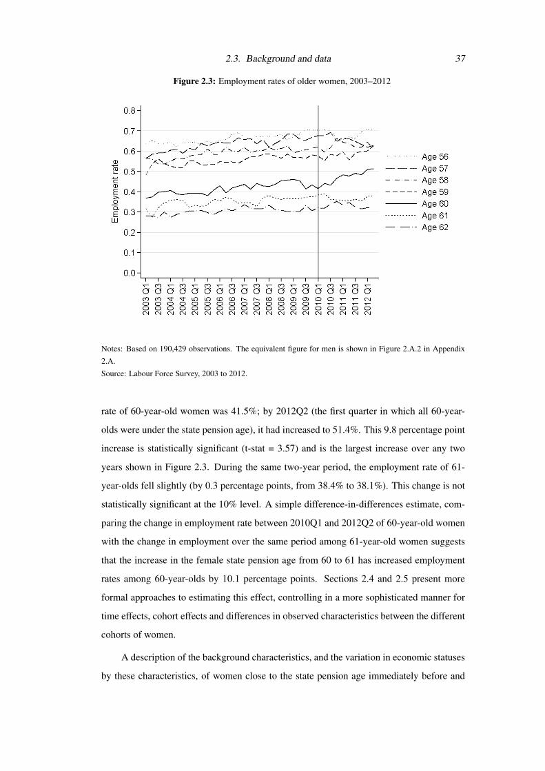
2.3 Employment rates of older women, 2003–2012 . . . . . . . . . . . . . . 37
2.4 Economic activity of men (aged 55–69) with partners, prior to female state
pension age reforms (by partner’s age) . . . . . . . . . . . . . . . . . . . 39
2.A.1 Economic activity of men prior to female state pension age reform, by age 56
2.A.2 Employment rates of older men, 2003–2012 . . . . . . . . . . . . . . . . 57
2.B.1 Difference in average retirement age between 1949–50 cohort and other
cohorts . . . . . . . . . . . . . . . . . . . . . . . . . . . . . . . . . . . . 63
3.1 Pension income and pension wealth for a stylised DB pension scheme
member . . . . . . . . . . . . . . . . . . . . . . . . . . . . . . . . . . . 74
3.2 Pension income and pension wealth for a stylised DC pension scheme
member . . . . . . . . . . . . . . . . . . . . . . . . . . . . . . . . . . . 75
3.3 Proportion receiving jobseeker’s allowance and pension credit . . . . . . 77
3.4 Average health percentile, by age and sex . . . . . . . . . . . . . . . . . 88
3.5 Proportion who retire in next two years, by baseline age and sex . . . . . 97
3.6 Proportion of non-workers who were in work two years later . . . . . . . 98
3.7 Actual and predicted retirement hazards . . . . . . . . . . . . . . . . . . 104
3.8 Predicted effect of increasing the state pension age by one year on retire-
ment hazards . . . . . . . . . . . . . . . . . . . . . . . . . . . . . . . . 108
3.9 Predicted effect of increasing the state pension age by one year on fraction
remaining in work . . . . . . . . . . . . . . . . . . . . . . . . . . . . . . 110
4.1 Expectations questions show card . . . . . . . . . . . . . . . . . . . . . . 119
4.2 Self-reported expectations of surviving to age 75 . . . . . . . . . . . . . . 121
14 List of Figures
4.3 Whether report 0% or 100% chance of survival, by number of other focal
answers given . . . . . . . . . . . . . . . . . . . . . . . . . . . . . . . . 126
4.4 Comparison of life table and average self-reported probabilities of survival 133
4.5 Comparing historic average chances of rain to mean self-reported probab-
ilities . . . . . . . . . . . . . . . . . . . . . . . . . . . . . . . . . . . . . 135
4.6 Fraction of respondents dying by age 75, by self-reported chances of dying
before age 75 . . . . . . . . . . . . . . . . . . . . . . . . . . . . . . . . . 137
4.7 Fraction of respondents dying within ten years, by self-reported chances
of dying by age 75 . . . . . . . . . . . . . . . . . . . . . . . . . . . . . . 138
4.8 Comparison of 2006 official life tables and median self-reported survival
curves . . . . . . . . . . . . . . . . . . . . . . . . . . . . . . . . . . . . 150
4.9 Comparison of alternative mortality curves for 25 year-old men . . . . . . 153
4.10 Comparison of alternative mortality curves for 65 year-old men . . . . . . 154
4.11 Consumption and asset profiles from a simple life-cycle model with altern-
ative assumptions about survival . . . . . . . . . . . . . . . . . . . . . . . 155
4.12 Consumption and asset profiles from a simple cake-eating model with al-
ternative assumptions about survival . . . . . . . . . . . . . . . . . . . . 156
4.A.1 Cumulative distribution of minimum probability reported . . . . . . . . . 160
4.A.2 Cumulative distribution of maximum probability reported . . . . . . . . . 161
4.A.3 Cumulative distribution of range of probabilities reported . . . . . . . . . 161
5.1 Self-assessed risk tolerance, by quintile of deviation between own and
age/sex group average expectations of survival . . . . . . . . . . . . . . . 196
5.2 Measured risk tolerance, by quintile of deviation between own and age/sex
group average expectations of survival . . . . . . . . . . . . . . . . . . . 197

List of Tables
2.1 Distribution of wealth among women born between April 1949 and March
1952 . . . . . . . . . . . . . . . . . . . . . . . . . . . . . . . . . . . . . 33
2.2 Economic activity of women born April 1949 to March 1952 . . . . . . . 38
2.3 Effect of increasing the state pension age from 60 to 61 on women’s em-
ployment . . . . . . . . . . . . . . . . . . . . . . . . . . . . . . . . . . . 43
2.4 Effect of increasing the state pension age from 60 to 61 on women’s em-
ployment for different subgroups . . . . . . . . . . . . . . . . . . . . . . 45
2.5 Effect of increasing the state pension age from 60 to 61 on women’s eco-
nomic status . . . . . . . . . . . . . . . . . . . . . . . . . . . . . . . . . 48
2.6 Effect of increasing partner’s state pension age on men’s economic status . 50
2.7 Effect of increasing female state pension age on employment of couples . 51
2.A.1 Number of women observed above and below state pension age . . . . . . 58
2.A.2 Effect of state pension age on female employment: OLS regression . . . . 59
2.A.3 Estimated difference between participation tax rate below and above the
state pension age . . . . . . . . . . . . . . . . . . . . . . . . . . . . . . 60
2.A.4 Effect of female state pension age on male employment: OLS regression . 61
3.1 Variation in pension accrual over and above scheme type . . . . . . . . . 76
3.2 Characteristics of workers and non-workers (men, 50–69) . . . . . . . . . 84
3.3 Characteristics of workers and non-workers (women, 50–69) . . . . . . . 85
3.4 Comparing those who do/do not attrit (male workers, 50–69) . . . . . . . 86
3.5 Comparing those who do/do not attrit (female workers, 50–69) . . . . . . 87
3.6 First principal component of health: men and women . . . . . . . . . . . 89
3.7 Distribution of earnings, pension wealth and accrual measures . . . . . . 94
3.8 Probability that men move out of work (random effects probit) . . . . . . 101
3.9 Probability that women move out of work (random effects probit) . . . . . 103

16 List of Tables
3.10 Probability of leaving work: effect of the option value over time . . . . . 106
3.11 Probability of leaving work: effect of the option value for different health
quintiles . . . . . . . . . . . . . . . . . . . . . . . . . . . . . . . . . . . 106
4.1 Self-reported probabilities of surviving to some older age . . . . . . . . . 120
4.2 Questions about expectations of the future asked in ELSA . . . . . . . . . 120
4.3 Reported chance of surviving to age 75 . . . . . . . . . . . . . . . . . . . 124
4.4 Deviation of self-reported chance of survival from age/sex group average
(men) . . . . . . . . . . . . . . . . . . . . . . . . . . . . . . . . . . . . 127
4.5 Deviation of self-reported chance of survival from age/sex group average
(women) . . . . . . . . . . . . . . . . . . . . . . . . . . . . . . . . . . . 130
4.6 How well does self-reported life expectancy predict 10-year mortality?
(men) . . . . . . . . . . . . . . . . . . . . . . . . . . . . . . . . . . . . 139
4.7 How well does self-reported life expectancy predict 10-year mortality?
(women) . . . . . . . . . . . . . . . . . . . . . . . . . . . . . . . . . . . 142
4.8 Expectations of surviving to age 75/80 in wave 3 . . . . . . . . . . . . . 148
4.9 Expectations of surviving to age 85 in wave 3 . . . . . . . . . . . . . . . 148
4.10 Estimated individual-specific survival curve parameters . . . . . . . . . . 149
5.1 Demographic characteristics . . . . . . . . . . . . . . . . . . . . . . . . 176
5.2 Health characteristics . . . . . . . . . . . . . . . . . . . . . . . . . . . . 177
5.3 Parents’ mortality . . . . . . . . . . . . . . . . . . . . . . . . . . . . . . 178
5.4 Positive correlation test: bivariate probit . . . . . . . . . . . . . . . . . . 185
5.5 Positive correlation test: correlation coefficients from bivariate probit . . . 188
5.6 Positive correlation test: probit of survival on annuity holdings . . . . . . 188
5.7 Relationship between annuity purchase and expectations of survival . . . 189
5.8 Relationship between annuity purchase and expectations of survival (part
I) . . . . . . . . . . . . . . . . . . . . . . . . . . . . . . . . . . . . . . . 192
5.9 Relationship between annuity purchase and expectations of survival (part
II) . . . . . . . . . . . . . . . . . . . . . . . . . . . . . . . . . . . . . . 193
5.A.1 Positive correlation test: full results from probit of survival on annuity
holdings . . . . . . . . . . . . . . . . . . . . . . . . . . . . . . . . . . . 200

List of Tables 17
5.A.2 Relationship between annuity purchase and expectations of survival (full
results) . . . . . . . . . . . . . . . . . . . . . . . . . . . . . . . . . . . . 202


Chapter 1
Introduction
This thesis contains four self-contained papers, each of which uses applied microecono-
metric techniques to examine questions relating to how individuals make financially-related
decisions at the end of working life and in early retirement. This work exploits the unique
combination of institutional framework and data available in the United Kingdom (UK) to
shed new light on these important issues.
Individuals’ decisions and private markets are playing an increasingly important role in
many developed countries in determining the financial well-being of people in later life. As
life expectancies have increased, fertility rates have fallen and the post-war baby boom gen-
eration has moved towards retirement, there has been growing pressure on public budgets,
making it increasingly hard to meet the rising pension and healthcare needs of the expanding
older population. As a result, there has been greater focus on how private provision might
ease the burden on the state, while ensuring that individuals continue to enjoy a decent
standard of living in later life.
Understanding whether and how individuals will provide for their retirements, how
they might react to policy changes and whether there is a need for further government in-
tervention requires an understanding of how individuals behave and how the markets they
interact with operate. This thesis contributes to that understanding by using detailed house-
hold microdata to examine what factors affect the timing of retirement, how individuals’
expectations of their own longevity affect their behaviour and examining the importance of
asymmetric information in the market for annuities.
1.1 Pensions and the timing of retirement
Pensions – both those provided by the state and those offered by employers – have, in the
post-World War II era, been found to play an important part in affecting when people leave

20 Chapter 1. Introduction
the labour market. Such schemes both intentionally (Lazear, 1979) and perhaps unintention-
ally influence when people choose to retire. An extensive economic literature has grown up
examining how individuals respond to the financial and non-financial incentives provided
by public and occupational pensions. One strand of this literature has sought to estimate
how responsive individuals’ retirement decisions are to financial incentives from pension
schemes, using both full dynamic programming models (for example Rust, 1989; French,
2005) and more reduced form approaches (Gruber and Wise, 2004).
One factor that has been identified as being important is specific focal ages (in par-
ticular, early and normal retirement ages) within public and occupational pension schemes.
This has led to a stream of work that has sought to quantify the effect of changing these
focal changes and understand what might be driving this effect. Early papers in this liter-
ature conducted ex ante simulations of these types of policy changes (Fields and Mitchell,
1984; Gustman and Steinmeier, 1985; Rust and Phelan, 1997; Coile and Gruber, 2000).
Since then a number of papers have evaluated the effect of these types of reforms in
practice across several countries, including Germany (Borsch-Supan and Schnabel, 1999),
the United States (Mastrobuoni, 2009), Switzerland (Hanel and Riphahn, 2012), Austria
(Staubli and Zweimuller, 2013) and Australia (Atalay and Barrett, 2015). While the ex ante
simulations suggested that the effects could be quite large, the ex post evaluations have sug-
gested even larger effects. A number of papers have examined the role that signals and/or
norms created by these focal ages might play in explaining the latter result (Lumsdaine,
Stock, and Wise, 1996; Kopczuk and Song, 2008).
Chapters 2 and 3 contribute to this existing literature by examining the responsiveness
of retirement behaviour to financial incentives and changing early retirement ages in a con-
text (the UK) where there is only a very weak relationship (in theory) between these incent-
ives in the pension system and labour supply incentives. The UK has been in the vanguard
of efforts to remove the direct link between incentives to claim a pension and incentives to
exit the labour market. For example, in 1989 the UK government removed the ‘earnings
test’ for receipt of the state pension (meaning that the amount of pension income received
was no longer reduced if the recipient had other earnings) and in 2006 it became possible
for individuals to draw a pension from their employer’s occupational pension scheme while
continuing to work for the same employer.
Chapter 2 uses a difference-in-differences approach to evaluate the impact of increas-

1.2. Expectations of survival and economic behaviour 21
ing the early retirement age for women in the UK state pension system from 60 to 61. This
occurred between 2010 and 2012. We find that this reform increased the employment rate
of women at the age of 60 by 7.3 percentage points and increased the employment rate of
affected women’s husbands by 4.2 percentage points. This finding adds to what has been
learnt from similar reforms in other countries by demonstrating that large changes in retire-
ment behaviour are possible even in a policy environment where there is only a very weak
relationship in theory between the date at which a public pension can be claimed and labour
force participation.
Evidence from subgroup analysis suggests that the effect seen for women is most likely
driven by the signals provided by the early retirement age. We find no evidence that credit
constraints, wealth effects or changes in the marginal financial incentives to work induced
by the policy can explain the changes in behaviour that were seen. We also conclude that
the response among male partners reflects complementarities in leisure within couples dom-
inating any substitution between the labour supply of husbands and wives.
Chapter 3 uses an option value model to examine how responsive older men and wo-
men’s labour supply is in England to the dynamic financial incentives provided by the pen-
sion, tax and benefit systems. I find that these dynamic financial incentives do have a stat-
istically and economically significant effect on labour force participation – despite the weak
links, in theory, between incentives to draw a pension and incentives to work.
However, I also find that these financial incentives cannot explain the spikes in retire-
ment rate at ages 60 (for women) and 65 (for men and women) that are observed in practice.
Furthermore, using my model to simulate the effect of increasing the early retirement age
in the state pension system suggests that this reform would increase employment rates of
older women by only around 3 percentage points if the effect was solely driven by changes
in the dynamic financial incentives. This suggests (as Chapter 2 also concludes) that other
factors – beyond the direct financial incentives – are important in explaining how women
have responded to this reform in the UK.
1.2 Expectations of survival and economic behaviour
The economic literature in this area, including my own analysis in Chapters 2 and 3, has
taken as its starting point some version of the life cycle model, which has formed the
backbone of the economic literature seeking to explain individuals’ decisions about con-
sumption, saving and labour supply over their lifetimes (Fischer, 1930; Modigliani and

22 Chapter 1. Introduction
Brumberg, 1954). One important aspect of such models is the uncertain lifetime that indi-
viduals face (Yaari, 1965). Most life-cycle models assume that individuals face the average
age- and sex-specific survival probabilities in their country and that they have rational ex-
pectations about their chances of survival (see, for example, Rust and Phelan, 1997). How-
ever, both of these are strong assumptions.
In Chapter 4 I show that, although individuals seem to have a good idea of how their
potential longevity compares to that of other people of their age and sex, they do not have
a good understanding of the shape of the survival curve that they face. In particular, I show
that most individuals perceive that their survival curve is much ‘flatter’ than actuarial estim-
ates suggest – that is, they appear to under-estimate the chance of surviving to younger ages
but over-estimate the chance of surviving to very old age. This has potentially important
implications for how individuals behave. This phenomenon of flatter survival curves has
been identified in other contexts before (Hamermesh and Hamermesh, 1983; Hamermesh,
1985; Ludwig and Zimper, 2013). Chapter 4 confirms that this is also seen in the UK and
presents new results on how this could affect economic decisions.
Using two simple models, I demonstrate that this misperception of survival chances
could help explain a number of puzzling aspects of individuals’ behaviour. In particular, I
show that it could help rationalise why individuals undersave for retirement, why consump-
tion drops sharply after retirement (Banks, Blundell, and Tanner, 1998), why demand for
annuities is lower than standard models suggest it should be (Fang, 2014) and why wealth
decumulation in later old age is so slow (De Nardi et al., 2010; Blundell et al., 2016).
Another area in which individuals’ knowledge of their potential longevity is import-
ant is in their interaction with private insurance markets – in particular, annuity and life
insurance markets. Private information about risk type can affect the existence, nature and
efficiency of the equilibrium in these markets (Rothschild and Stiglitz, 1976). Previous
work has demonstrated that adverse selection does (or at least did) exist in the UK annuity
market in the 1980s and 1990s (Finkelstein and Poterba, 2002, 2004, 2014). However, this
earlier work, which used data from insurance companies, was not able to establish whether
this adverse selection was active or passive. In Chapter 5 I shed interesting new light on this
question using detailed household survey data. The analysis presented is only possible with
the unique combination of data and institutional framework that exists in England. I find
that adverse selection exists in this market, even after taking into account the more extensive

1.2. Expectations of survival and economic behaviour 23
underwriting criteria that have been adopted over the last decade. Furthermore, I show that
this selection is (at least in part) active – annuity purchasers live for longer than otherwise
similar non-annuitants and they anticipate this.
The findings presented here suggest a number of potentially interesting avenues for
future work. Chapters 2 and 3 both suggest that focal ages and signals about when one
can claim a pension affect labour force participation, even when these are not accompan-
ied by any strong financial incentives. However, the data and techniques used here shed
only limited light on the mechanisms through which this effect works. New data that will
become available over the next few years should provide opportunities for exploring these
mechanisms more thoroughly.
The analysis presented in Chapter 4 suggests that heterogeneity in survival expect-
ations and systematic deviations of individuals’ expectations from life table values could
help to explain some facets of behaviour. It would be worthwhile trying to use these data on
expectations to estimate a more elaborate life cycle model to see how this affects estimates
of other important preference parameters, such as discount rates and risk aversion.
Chapter 5 shows that active adverse selection occurs in the UK annuity market. There
is further work to be done to understand the nature of equilibrium in this market when it
appears that buyers and sellers hold different beliefs about the risks facing the pool of poten-
tial purchasers. Further information (or strong assumptions) about risk preferences are also
required to estimate the welfare loss from adverse selection in this market. Understanding
more about the equilibrium in this market could be very important as many countries look
to expand the role of individually purchased annuities in providing longevity insurance.
The approach I have taken in this thesis focusses mainly on individual decision-
making. However, a number of the findings suggest further questions about collective de-
cision making within families, which could be explored further. Chapter 2 suggests that
complementarities in leisure within couples may be important. The evidence in Chapter 4
suggests that men’s and women’s expectations of survival are closer to one another than ob-
jective estimates suggest, which hints at potentially interesting questions about how people
form these expectations and whether expectations are too highly correlated within couples.
These possible avenues for future work are discussed in more detail in Chapter 6,
which offers some concluding remarks.


Chapter 2
Increasing the female state pension age in
the UK: Effects on labour supply of older
women and their husbands
2.1 Introduction1
Governments across the developed world have, over recent decades, legislated for increases
in the early and normal claiming ages that apply to public pension schemes. Such policies
have often been adopted with the explicit intention of strengthening the public finances in
the face of rapidly ageing populations – not only by reducing payments to pensioners but
also by increasing average retirement ages and thus generating additional tax revenues. In
this paper we exploit a recent reform of the state pension age for women in the UK to
estimate the effect on their labour force participation. This provides an important addition
to the small existing empirical literature on this topic (Staubli and Zweimuller, 2013; Atalay
and Barrett, 2015) by examining such a reform in the context of a public pension system
that provides minimal financial incentives to exit work at the early retirement age.2 By
1This chapter is co-authored with Jonathan Cribb and Carl Emmerson and is an amended version of theworking paper Cribb, Emmerson, and Tetlow (2013). We are grateful to James Banks, Richard Blundell, IanCrawford, Monica Costa Dias, Eric French, Robert Joyce and Bansi Malde for comments, and to James Brownefor assistance with calculating participation tax rates using TAXBEN. This paper has also benefited greatlyfrom comments received from participants at the following conferences and seminars: Royal Economic Societyannual conference (April 2013); NBER Summer Institute (July 2013); Work, Pensions and Labour EconomicsStudy Group conference (July 2013); Netspar International Pensions Workshop (January 2014); Society ofLabor Economists annual conference (May 2014); Institute for Evaluation of Labour Market and EducationPolicy (IFAU), Uppsala, Sweden; Superintendencia de Pensiones, Santiago, Chile; and at the Institute for FiscalStudies.
2The state pension age is actually the only focal age in the UK state pension system, there is no separatenormal retirement age. However, the state pension age operates like an early retirement age in other systems inthat it is the earliest point at which someone can start receiving a state pension – there is no option for claimingearlier.

26 Chapter 2. Increasing the female state pension age
examining how the labour supply of women’s partners responds to an increase in the female
state pension age, this paper also contributes to the literature on complementarities of leisure
within couples.
In 1995, the UK government legislated to increase the state pension age (that is, the
earliest age at which a pension can be claimed from the state) for women from 60 to 65.
This was legislated to happen between 2010 and 2020. This paper uses evidence on labour
market behaviour in the UK between 2010 and 2012 to examine what impact increasing the
state pension age from 60 to 61 has had on the economic activity of the affected cohorts of
women and their partners.
Women’s economic activity could be affected by an increase in the state pension age
through four main mechanisms. First, increasing the state pension age will have some effect
on individuals’ marginal financial incentives to work, through changing marginal tax rates
and eligibility for out-of-work benefits. This channel will be significantly less important in
the UK than it is in some other countries because there is no earnings test for state pension
receipt in the UK.
Second, the increase reduces the length of time that individuals receive state pension
income and thus reduces their lifetime wealth; this will tend to increase labour supply. How-
ever, if those affected were forward looking and well informed, this response might have
manifested as soon as the legislation was passed. Since this policy reform was announced
15 years in advance, we might expect adjustments in employment rates around the state
pension age to be quite small, as individuals have had a considerable period of time over
which to adjust their behaviour. However, evidence suggests that – even many years after
the legislation was passed – many of the women affected were unaware of it. Crawford and
Tetlow (2010) – using data collected in 2006–07 – find that, at that time, six-in-ten of those
women who face a state pension age somewhere between 60 and 65 were unaware of their
true state pension age. This suggests that some women may face a significant shock as they
approach their state pension age and thus may have to adjust their behaviour sharply over
a short period of time. Previous evidence suggests that individuals respond most strongly
to what they believe the rules of the system are, even if their beliefs are incorrect (Bottazzi,
Jappelli, and Padula, 2006; Coppola and Wilke, 2014).
Third, individuals who are credit constrained may have to continue working during the
period when they are no longer able to receive their state pension in order to finance their

2.1. Introduction 27
consumption.
Finally, the state pension age may provide a signal about the ‘appropriate’ age at which
to retire. The UK Department for Work and Pensions writes to each person who is entitled
to a state pension four months before they become eligible to tell them how to claim. There-
fore, even if the person is entirely unaware of their eligibility date before this, this commu-
nication may provide a strong signal. If the state pension age does provide such signals,
moving this age could have a greater impact on employment rates than the pure financial
incentives would suggest.
We may see a correlation between the timing of retirement of women and their hus-
bands for one or more of three possible reasons. First, couples may experience correlated
shocks, which could cause them to retire at the same time. Second, couples may have a
preference for spending time together (i.e. complementarities of leisure), which also cause
them to retire at the same time. Third, labour earnings of one member of the couple may be
a substitute for earnings of the other partner, suggesting that the two members of a couple
would retire at different times from one another. The difference-in-differences estimation
technique we use is likely to be robust to the first channel. However, we might expect either
or both of the other two channels to be important in determining how affected women and
their partners responded to the increase in the female state pension age. On the one hand,
if couples enjoy spending their retirement together, husbands may retire later if their wives
are induced to retire later – suggesting we would see an increase in both male and female
labour supply within the same families. On the other hand, if the policy change increases
credit constraints or imposes a wealth or income shock on the couple, it may be that the
husband’s labour supply rather than the wife’s responds to compensate – suggesting that
we might see an increase in female labour supply in some families but an increase in male
labour supply in others.
We identify the impact of increasing the state pension age (on the labour force parti-
cipation of women and their male partners) by comparing cohorts who face different state
pension ages, while allowing for a flexible specification of cohort, age and time effects.
However, the specification we have chosen limits us to identifying only those effects that
manifest between the old and new state pension ages; other differences in employment rates
between treated and control cohorts that occur before or after these points will be subsumed
into the cohort effects that are included in our specification. For this reason, the effect we

28 Chapter 2. Increasing the female state pension age
identify – which is sizeable – could be considered a lower bound on the true response to the
policy. One reason to think that significant effects may not manifest at earlier ages is that
changing the state pension age only affects marginal financial incentives to work between
the old and new state pension ages, and not at earlier ages – unlike the effect of a change in
the normal retirement age. The effect we estimate may not, however, be a true lower bound
since it is the short-run effect, which could be larger than the long-run effect if, for example,
individuals did not fully anticipate the policy change or smaller if, for example, it takes time
for social norms to adjust to the reform.
We find that employment rates of women at age 60 increased by 7.3 percentage points
when the state pension age was increased to 61; this result is statistically significant at the
1% level. This is equivalent to about a one month increase in the average retirement age.
The result is robust to a number of specification tests, including using a linear probability
model rather than probit, variations in the sample chosen to exclude repeat observations on
the same individuals, and using a wild cluster bootstrap procedure to account for potential
serial correlation in employment shocks (as suggested by Cameron, Gelbach, and Miller,
2008).
We find that employment rates among affected women’s partners increased by around
4.2 percentage points (with this result being statistically significant at the 5% level and the
point estimate being reasonably robust to different specifications). Looking at the employ-
ment of both members of couples, we find that – among couples where the wife is aged
around the state pension age – the increase in the female state pension age has led to an in-
crease in the proportion of two-earner couples (5.4 percentage points) and a decrease in the
fraction of couples where neither is in paid work (4.7 percentage points) but no significant
change in the fraction of couples where only the husband or only the wife is in paid work.
We interpret this as evidence that complementarities of leisure within couples dominate any
substitution that happens between labour supply of members of couples in response to the
policy.
Subgroup analysis provides some tentative evidence on which mechanisms may be
important in explaining the changes in behaviour that we observe. There is no significant
difference in the response among owner-occupiers and renters, which we interpret as sug-
gestive evidence that credit constraints may not be the primary driver. We also find that the
increase in employment is smallest among those who are likely to have faced the largest
2.2. Related literature 29
decrease in participation tax rate at age 60 due to the increase in the state pension age.
Although the point estimates are not statistically significantly different across groups, this
is suggestive that changing marginal financial incentives are also not a major explanatory
factor. In addition, the cohort fixed effects included in our model control for differences in
state pension wealth across cohorts that are a direct result of the increase in the state pension
age. Therefore, unless wealth effects affect behaviour in a non-linear way that is not allowed
for in our model, we can also rule out that these are the major driving force of the response
we see. Together these suggest that the role of the state pension age in providing a signal
about the appropriate retirement age may well be an important reason why increasing the
state pension age feeds through into such a sizeable increase in labour force participation.
The remainder of this chapter proceeds as follows. Section 2.2 provides a summary of
the related literature. Section 2.3 describes the institutional setting, the policy reforms we
exploit and the data we use and presents evidence on how employment rates changed around
the state pension age prior to the reform. Section 2.4 describes our empirical strategy and
Section 2.5 presents the results. Section 2.6 concludes.
2.2 Related literature
Gruber and Wise (2004) surveyed evidence on eleven developed countries and highlighted
the fact that labour force exits are concentrated around legislated early and normal retire-
ment ages and tend to be larger than can be explained by the pure financial incentives as-
sociated with retiring at these ages. Most of the early papers that attempted to simulate
the impact of moving these early and normal retirement ages on labour force participation
relied on using out-of-sample predictions. Papers simulating changes in early and nor-
mal retirement ages in the US suggested quite large effects on retirement ages (Fields and
Mitchell, 1984; Gustman and Steinmeier, 1985; Rust and Phelan, 1997; Coile and Gruber,
2000; French, 2005). For the UK, Blundell and Emmerson (2007) estimate that a three-year
increase in the state pension age for both men and women (and assuming that defined bene-
fit occupational pension schemes respond with a three-year increase in their normal pension
ages as well) would increase retirement ages by between 0.4 and 1.8 years, depending on
the specification used.
However, while the effects estimated in these ex ante simulations were quite large,
if anything the results of ex post evaluations suggest even larger effects. One of the first
papers to examine ex post the impact of a change in early retirement ages (ERAs) was
30 Chapter 2. Increasing the female state pension age
Borsch-Supan and Schnabel (1999), who looked at evidence from the reduction in the earli-
est age of pension receipt in Germany from 65 to 63 in 1972. Prior to this reform, the
vast majority of men in Germany retired at age 65, whereas after the reform there was a
significant shift towards retiring at age 63. More recently, there have been a growing num-
ber of reforms around the world, which have increased pension ages. Therefore, ex post
evaluations have become more common in the literature, although almost all of these have
focused on changes to normal, rather than early, retirement ages (including, among others,
Mastrobuoni, 2009; Hanel and Riphahn, 2012; Behagel and Blau, 2012; Lalive and Staubli,
2014).
The two major exceptions are Staubli and Zweimuller (2013) and Atalay and Barrett
(2015), who examine the effect of changes in ERAs. The former use administrative data
and employ a similar estimation strategy to that used in this paper to examine an increase
in the ERA in Austria. They find that a one year increase in the ERA led to an increase in
employment rates of 9.75 percentage points for affected men and by 11 percentage points
for affected women, with increases in unemployment rates of a similar size. However, the
Austrian state pension system is different from the UK (and a number of other countries’
systems) in several important ways. First, individuals’ pension benefits are completely with-
drawn if their earnings exceed around $500 a month. Second, although the Austrian system
provides some increase in pension income for delayed drawing, this is done at a less than
actuarially fair rate. Third, the Austrian state pension provides a very high level of earnings
replacement (according to Staubli and Zweimuller (2013) the average net replacement rate
of pre-retirement earnings is 75%); public pensions, therefore, provide the main source of
income for most pensioners in Austria.
Atalay and Barrett (2015) examine the effect of an increase in the earliest age at which
women can access the Australian Age Pension. They find, using cross-sectional survey data,
that a one year increase in the eligibility age induced a 12–19 percentage point increase in
female labour supply. In Australia (unlike in the UK and many other countries) receipt
of the state pension is means-tested against income, which provides a strong incentive for
many Australians to retire at the point at which they can become eligible for the pension.
Importantly, our paper adds to the evidence provided by Staubli and Zweimuller (2013)
and Atalay and Barrett (2015) by providing the first evidence from a change in ERA in the
context of a system (the UK system) in which there are not strong financial disincentives to

2.3. Background and data 31
working beyond the ERA, and where private pension saving provides a significant fraction
of retirement income for many people. In these respects, the UK pension system is more
similar to that in the US than either the Austrian or the Australian systems.
There is mixed evidence from previous work about the importance for behaviour of
signals around retirement ages. Lumsdaine, Stock, and Wise (1996) found that there are
excess peaks in retirement in the United States at age 65 (the Social Security normal retire-
ment age at the time), over and above those explained by the financial incentives generated
by Social Security and Medicare, implying that there is an important signal to retire at 65.
Kopczuk and Song (2008) find a significant pattern of individuals claiming Social Security
in January or on their birthday, either of which might be considered a simple focal point or
signal. Behagel and Blau (2012) conclude that non-standard preferences can explain why
older Americans responded so strongly to the increase in the normal retirement age in So-
cial Security that occurred in the early 2000s. Conversely, others have found evidence to the
contrary – for example, Asch, Haider, and Zissimopoulos (2005), who examined the retire-
ment behaviour of civil service employees in the US, who face different financial incentives
to retire from the majority of the population who are covered by Social Security.
Several papers have examined the importance of complementarities in leisure of
couples in affecting retirement ages (Baker, 2002; Coile, 2004; Banks et al., 2010; Stan-
canelli, 2012). The most closely related to our study is Banks, Blundell, and Casanova
(2010), who exploit differences in pension claiming ages for women in the US and UK to
identify the impact of a woman leaving work on her (male) partner’s employment and find
significant evidence of joint retirement within couples. We exploit the differences in pen-
sion claiming ages for women induced by the 1995 reforms to identify whether there has
been any knock-on effect on the labour supply of male partners.
2.3 Background and data
2.3.1 Institutional details
The state pension age in the UK is the earliest age at which individuals can receive a state
pension. There is no earnings test for receipt of the state pension (that is, the amount
received is not reduced if the individual also has earned income)3 but individuals do receive
an actuarial adjustment of benefits if they delay claiming beyond the state pension age.
3The earnings test was abolished in 1989. Disney and Smith (2002) examine the labour supply impact ofremoving the earnings rule.
32 Chapter 2. Increasing the female state pension age
Those not claiming the state pension when they reach the state pension age receive a 10.4%
increase in their income for each year that they delay claiming.4 However, in practice, very
few people choose to delay claiming.
The UK state pension consists of two parts. The first-tier pension (known as the Basic
State Pension) is based on the number of years (but not on the level) of contributions made.5
The second-tier pension is related to earnings across the whole of working life (from 1978
onwards); enhancements are also awarded for periods spent out of work due to some formal
caring responsibilities since April 2002. However, historically, the majority of employees
have chosen to opt out of this second-tier pension in return for a government contribution
to a private pension scheme.6
A full Basic State Pension in 2012–13 was worth £107.45 a week (17% of average
full-time weekly earnings).7 Most men and women now reaching the state pension age can
qualify for the full award. The second-tier pension scheme replaces 20% of earnings within
a certain band. The maximum total weekly benefit that could be received from the second-
tier pension was around £160. However, since most employees opted out of the second-tier
pension scheme in the past, the majority of pensioners receive far less than this from the
state.
Between 1948 and April 2010, the state pension age was 65 for men and 60 for women.
The Pensions Act 1995 legislated for the female state pension age to rise gradually from 60
to 65 over the ten years from April 2010, with the state pension age rising by one month
every two months for ten years. As a result, women born after April 1950 have a state
pension age of greater than 60.8 This is shown in Figure 2.1. The total loss from a one-year
increase in the state pension age is £5,587 for a woman who qualifies for a full Basic State
Pension and no additional pension, rising to around £14,000 for a woman who qualifies for
a full Basic State Pension and a full additional pension entitlement.9
4This adjustment is prorated for partial years of deferral; each 5 weeks of deferral results in a 1% increasein pension income.
5Periods in receipt of certain unemployment and disability benefits and periods spent caring for children oradults can also boost entitlement.
6A full description of the UK state pension system can be found in Bozio, Crawford, and Tetlow (2010).7Women approaching the state pension age actually earn, on average, much less than this and are more
likely to work part time. Median earnings for 59 year old women who were in work in the two years prior tothe increase in the state pension age were £254 per week.
8To our knowledge no occupational pension schemes adjusted their normal pension ages in line with thechange in the female state pension age. Until very recently, the most common normal pension ages were 60 inpublic sector schemes and 65 in private sector schemes. We are not aware of any schemes that apply a differentnormal pension age to male and female scheme members.
9This is based on a full Basic State Pension and a maximum State Second Pension entitlement being lost

2.3. Background and data 33
Figure 2.1: Female state pension age under different legislation
Source: Pensions Act 1995, schedule 4 (http://www.legislation.gov.uk/ukpga/1995/26/
schedule/4/enacted); Pensions Act 2007, schedule 3 (http://www.legislation.gov.uk/
ukpga/2007/22/schedule/3); Pensions Act 2011, schedule 1 (http://www.legislation.gov.
uk/ukpga/2011/19/schedule/1/enacted).
Table 2.1: Distribution of wealth among women born between April 1949 and March 1952
£ thousands Mean 25th Median 75th
percentile percentile
State pension wealth (individual) 128.0 98.8 131.4 160.5State pension wealth (family) 226.4 169.1 235.9 294.3
Private pension wealth (individual) 90.2 0.0 23.4 104.9Private pension wealth (family) 248.2 21.6 136.3 328.8
Net financial wealth (family) 84.3 1.4 24.2 90.6Net housing wealth (family) 201.8 85.0 180.0 280.0Other physical wealth (family) 56.1 0.0 0.0 4.5
Total net wealth (family) 820.5 399.6 660.5 1,026.3
Notes: Sample includes all ELSA core sample members born between 1 April 1949 and 31 March 1952. Sample
size=746. Weighted using cross-sectional weights.
Source: English Longitudinal Study of Ageing, wave 5 (2010–11).
34 Chapter 2. Increasing the female state pension age
State pension entitlements make up a significant fraction of total retirement resources
for some individuals, while for others they are much less important. Table 2.1 shows stat-
istics on the distribution of different types of wealth among the cohorts of women that are
the focus of this paper. On average, these cohorts had accrued about £130,000 of state pen-
sion entitlements by 2010; this figure is calculated as the present discounted value of the
estimated future stream of state pension income. However, these women’s mean total fam-
ily wealth is just over £800,000. Women’s own state pension wealth accounted on average
for one-quarter of their family’s total wealth but for one-in-nine women their state pension
wealth accounts for more than half their family’s total wealth.
Some other features of the tax and benefit system also change when an individual
reaches the state pension age and potentially influence incentives to remain in paid work.
First, employees are no longer liable for employee National Insurance contributions (i.e.
payroll taxes decline); this increases the financial incentive to be in paid employment.
Second, instead of being able to claim the main working-age unemployment and disabil-
ity benefits,10 households with one member above the female state pension age become
eligible to claim the means-tested Pension Credit Guarantee. This is more generous than
the equivalent working-age benefits: not only is the amount received higher (£142.70 per
week, with greater amounts for those with disabilities) but there are also no requirements for
recipients to, for example, seek work or attend work-focused interviews. This reduces the
incentive for individuals to be in, or to seek, paid work after reaching state pension age. In
addition, state pension income will exhaust some or all of an individual’s income tax ‘per-
sonal allowance’ (that is, the amount of income that can be received tax free). Therefore,
the average rate of income tax on an individual’s earnings may actually increase at the state
pension age if receipt of state pension income causes them to be pushed into a higher tax
bracket. As we show in Section 2.5.2, these different effects mean that some women face
a lower incentive to work (as measured by a participation tax rate) at the age of 60 when
the state pension age rises, while others see almost no change or an increased incentive to
work.11
for one year.10The main working-age unemployment benefit is known as Jobseeker’s Allowance (JSA) and is paid at a
rate of £71.00 per week. The main working-age disability-related benefit is known as Employment and SupportAllowance (ESA) and is paid at a rate of £99.15 per week.
11Those aged above the female state pension age are also eligible for the Winter Fuel Payment (which isworth £200 a year) and for free off-peak bus travel. The impact of these payments on labour supply incentivesis ambiguous but it is unlikely to be significant.

2.3. Background and data 35
2.3.2 Data
We use data from the UK’s Labour Force Survey (LFS).12 This is conducted on a quarterly
basis, with all individuals in a household followed for up to five consecutive quarters
(‘waves’) and with one-fifth of households being replaced in each wave. The sample size is
large – for example, during January to March 2012, 102,531 individuals were interviewed
from 43,794 households and the survey contains information on individual labour market
activities combined with background information such as sex, age, marital status, education
and housing tenure. Crucially for our study, the data contain month as well as year of birth,
and the large sample sizes mean relatively large numbers of individuals are observed from
each birth cohort at each age. For example, about 170 individuals born in the first quarter
to be affected by the reform (1950Q2) are observed in each quarter of the LFS data that we
use in our analysis (which runs from 2009Q2 to 2012Q2). Further details of the achieved
sample size by age and cohort are shown in Table 2.A.1 in Appendix 2.A.
Data from the LFS are used to produce internationally comparable unemployment stat-
istics using International Labour Organisation (ILO) definitions of employment and unem-
ployment. Therefore, we use ILO measures of economic activity in our analysis. Under
these definitions, an individual is categorised as employed if they do any paid work (as an
employee or self-employed) in the week of their interview, if they are temporarily away
from paid work or if they are on a government training scheme (although this last category
is rare for older people). Individuals are considered as being in full-time work if they work
30 or more hours in a usual week. If individuals are not in work, they are categorised as
either unemployed (looking for work in the last four weeks or waiting for a job to start and
they must be able to start work within the next two weeks), retired, sick or disabled, or a
residual category (these are all self-defined). Each individual is categorised as being in one
and only one of these categories.
The pattern of economic activity of older women by age is shown in Figure 2.2. This
uses LFS data pooled across the eight years before the female state pension age was in-
creased. The percentage of women in paid work (either full-time or part-time) declines
with age (which will be due to a combination of age and cohort effects). Between age 59
and age 60, there is a 13.7 percentage point drop in employment and a 23.5 percentage point
12We do not use data from the English Longitudinal Study of Ageing (ELSA), which was described inTable 2.1, as it does not yet provide sufficient observations of employment rates of older women since the statepension age started to increase. The sample size of women in the relevant cohorts is also much larger in theLFS than in ELSA.

36 Chapter 2. Increasing the female state pension age
Figure 2.2: Economic activity of women prior to state pension age reform, by age
Notes: Averages over the period 2003Q1 to 2010Q1. Based on 404,428 observations. The equivalent figure for
men is shown in Figure 2.A.1 in Appendix 2.A.
Source: Labour Force Survey.
increase in the percentage reporting themselves as retired. Both of these changes are bigger
than any of the changes observed between other consecutive ages. However, prior to the
female state pension age being increased, it was not possible to separate out the extent to
which this was an impact of hitting the state pension age as opposed to an impact of hitting
age 60.13
An initial indication of what the impact of increasing the state pension age on em-
ployment has been is provided by Figure 2.3. This shows how employment rates of older
women have evolved since 2003 by single year of age. While employment rates at each age
have generally been increasing over time (due, at least in part, to later cohorts of women
having greater labour force attachment), a particularly large increase has been observed for
60-year-old women from April 2010 onwards, which is when the state pension age started
to rise. In 2010Q1 (just prior to the increase in female state pension age), the employment
13One approach has been to assume a parametric relationship between labour market exit and age (forexample, a quadratic in age) and also allow for an additional impact of hitting the state pension age. Butthis assumes that all of the additional retirements that occur at age 60, over and above those explained by therelationship with age measured at earlier and later ages (and other covariates in the model), are due to this agebeing the state pension age. See, for example, Blundell and Emmerson (2007).
2.3. Background and data 37
Figure 2.3: Employment rates of older women, 2003–2012
Notes: Based on 190,429 observations. The equivalent figure for men is shown in Figure 2.A.2 in Appendix
2.A.
Source: Labour Force Survey, 2003 to 2012.
rate of 60-year-old women was 41.5%; by 2012Q2 (the first quarter in which all 60-year-
olds were under the state pension age), it had increased to 51.4%. This 9.8 percentage point
increase is statistically significant (t-stat = 3.57) and is the largest increase over any two
years shown in Figure 2.3. During the same two-year period, the employment rate of 61-
year-olds fell slightly (by 0.3 percentage points, from 38.4% to 38.1%). This change is not
statistically significant at the 10% level. A simple difference-in-differences estimate, com-
paring the change in employment rate between 2010Q1 and 2012Q2 of 60-year-old women
with the change in employment over the same period among 61-year-old women suggests
that the increase in the female state pension age from 60 to 61 has increased employment
rates among 60-year-olds by 10.1 percentage points. Sections 2.4 and 2.5 present more
formal approaches to estimating this effect, controlling in a more sophisticated manner for
time effects, cohort effects and differences in observed characteristics between the different
cohorts of women.
A description of the background characteristics, and the variation in economic statuses
by these characteristics, of women close to the state pension age immediately before and

38 Chapter 2. Increasing the female state pension age
Table 2.2: Economic activity of women born April 1949 to March 1952
Percentage of sample in each economic activity
Full Part Retired Unempl. Sick/ Other Ntime time disabled
Full sample 28.2 25.0 23.9 1.9 12.5 8.5 30,297
Single women 32.8 18.8 19.5 3.3 19.8 5.7 8,818Women with a partner 26.3 27.5 25.7 1.3 9.5 9.7 21,479
whose partner is older 25.1 26.6 27.2 1.2 9.7 10.1 15,955whose partner is younger 29.6 30.1 21.3 1.5 9.0 8.5 5,524
Rents house 20.5 15.3 18.3 3.5 31.5 10.9 5,853Owns house 30.0 27.3 25.2 1.5 8.0 8.0 24,444
Degree or other HE 34.7 26.4 25.9 1.8 5.7 5.5 8,416Secondary education 30.4 27.3 22.1 1.9 10.4 7.9 14,756No qualifications 15.8 18.6 25.2 2.0 24.9 13.5 7,125
Notes: Totals may not sum to 100 due to rounding.Source: Labour Force Survey, 2009 Q2 to 2012 Q2.
after it started to rise from age 60 is shown in Table 2.2. Among those not in paid work,
the most common reported activities are being ‘retired’, being ‘sick or disabled’ and ‘other’
(which most commonly refers to looking after the home or family). Relatively few wo-
men in this group report themselves as being unemployed. Full-time employment is more
common among single women than among those in couples. Those who own their own
home are much more likely to be in work (either full- or part-time) than those who rent
their home, while those in the latter group are relatively more likely to be unemployed or
sick/disabled (indeed, almost one-third of renters report being sick or disabled). Employ-
ment rates are positively correlated with levels of education, with those with lower levels
of education being more likely to report being sick/disabled or having ‘other’ as their main
economic activity.
The data also allow us to explore the impact of the increase in the female state pension
age on the labour market activity of the male partners of those directly affected by the
reform. Data from prior to the reform show that – among men aged 55 to 69 who are
partners of women aged between 50 and 69 – employment rates do typically fall as wife’s
age increases and the largest drop (of 7.2 percentage points) is between those whose female
partner is aged 59 and those whose female partner is aged 60 (see Figure 2.4).

2.4. Empirical methodology 39
Figure 2.4: Economic activity of men (aged 55–69) with partners, prior to female state pension agereforms (by partner’s age)
Notes: Averages over the period 2003Q1 to 2010Q1. Number of observations = 193,738.
Source: Labour Force Survey.
2.4 Empirical methodology
Using data on the labour market behaviour of women who face different state pension ages
allows us to estimate what impact increasing the state pension age for women from 60 to
61 has had on labour market behaviour. To do this, we employ a difference-in-differences
methodology. The ‘treatment’ (being under the state pension age) is administered at some
point to all women but since the reform was introduced is administered for longer to women
born more recently. Equation 2.1 sets out the specification we use to estimate the impact of
increasing the state pension age.
yict = α (underspaict)+ γt +λc +A
∑a=1
δa [ageict = a]+Xictβ + εict (2.1)
Our aim is to estimate the effect on an outcome, y, of being below (rather than above)
the state pension age. Fixed effects are used to control for time period (γt), cohort (λc)
and age. In other words, we assume that there are cohort- and time-constant age effects,
time- and age-constant cohort effects and age- and cohort-constant time effects. The last is

40 Chapter 2. Increasing the female state pension age
the usual common trends assumption required for identification in difference-in-differences
estimation. We might be particularly concerned about this identifying assumption being
violated in our application if the policy of interest has affected our control group through
general equilibrium effects in the labour market. For example, if increasing the state pension
age for younger cohorts led to more 60-year-olds wanting to remain in work, this could have
reduced employment opportunities for 61-year-olds. Such an effect would bias upwards
our estimated effect of increasing the state pension age on women’s employment rates. We
cannot rule out this possibility.
The age- and time-constant cohort effects control in a flexible way for underlying dif-
ferences in employment patterns between different cohorts of women. However, this comes
at the cost of subsuming within this ‘cohort effect’ any impact of the state pension age re-
form that manifests itself in time-constant changes in economic activity rates among the
affected cohorts before age 60.14,15
We also control for a vector of individual characteristics, X . These include education,
relationship status, housing tenure, ethnicity, geography, as well as partner’s age and part-
ner’s education for those with a partner – the full set of covariates included is laid out in
Table 2.A.2 in Appendix 2.A.
To estimate the impact on (male) partners’ outcomes, we use a similar specification.
The impact of increasing a woman’s state pension age on her partner’s economic activity is
estimated, controlling for the woman’s cohort, woman’s age and time in the same way that
we control for these when estimating the effect on female employment. Additional controls
are also used, which most importantly include controls for the man’s own age. We control
for the man’s age using a quadratic in age plus indicators for being aged over the female
state pension age and for being aged 65 or over.16 The identifying assumption is that – after
controlling for own age, partner’s age, time and cohort effects – any difference between
the employment rates of men with female partners who are aged above and below the state
14An alternative approach would have been to specify a functional form for the cohort effects and attributeany deviations from this pattern between cohorts who were affected by the 1995 legislation and those who werenot as being the result of the policy change. This is essentially the approach adopted by Mastrobuoni (2009).The results of an exercise along these lines are presented in Appendix 2.B. In summary, we find no evidencethat increasing the state pension age led to delayed retirement (and therefore increased labour supply) betweenthe ages of 55 and 59.
15Any other policy changes that affect cohorts (and their behaviour) differently, but in a time-constant way,will also be absorbed into these cohort effects. This could apply, for example, to the reforms legislated inPensions Act 2007, which changed the way that pension entitlements were calculated (in a way that made thesystem more generous on average) for all those born after 5 April 1950.
16The full specification as estimated by OLS is set out in Table 2.A.4 in Appendix 2.A.

2.5. Results 41
pension age is due to the impact of their partners reaching the state pension age. This
identifying assumption is cleaner than the one used in identifying the effect on women’s
economic activity. Whereas all women of the same age at a given time are either above
or below the state pension age, for men of a given age at a certain time, they may have a
partner who is either above or below the state pension age.
Our primary interest is in the effect of increasing the state pension age on employment.
This is estimated using both ordinary least squares (OLS) and a probit model, calculating
the average marginal effects of the treatment.17 However, we are also interested in the other
possible economic states. To assess these, multinomial probit models are used to examine
the impact of increasing the state pension age on:
1. Whether an individual is in full-time or part-time work or not in paid work
2. Whether an individual is in work, retired, sick or disabled, unemployed and a residual
category
Since the LFS tracks individuals over up to five consecutive quarters of data, our
sample contains multiple observations of the same individuals and so the observations are
not independent of one another. We control for this by clustering standard errors at the indi-
vidual level and also conduct a sensitivity analysis using only the first observation on each
individual. We show that these methods change the estimated marginal effect very little but
increase the standard errors as the sample size is substantially reduced. Our results are also
robust to allowing for serially correlated cohort-time shocks.
2.5 Results
2.5.1 Effect on women’s employment rates
All the models are estimated on data from 2009Q2 – one year before the state pension
age started to rise – to 2012Q2 the point at which the state pension age had reached 61.18
17Since being under the state pension age is a function of both a woman’s cohort and time, the variableunderspa is an interaction. In a non-linear model, calculating marginal effects on an interaction term doesnot produce a difference-in-differences treatment effect as it does in a linear model. To estimate the treatmenteffect in a non-linear model, we estimate the model and then, for each observation, look at the difference inthe predicted probability of employment if above and below the state pension age and then average across allobservations to calculate the average marginal effect across the whole distribution of other regressors.
18An alternative specification that we considered includes an additional two years of data prior to the reform(from 2007Q2 onwards) and more unaffected cohorts (born in 1947–48 and 1948–49).The benefit of includingmore data prior to the increase in the ERA is that helps to identify age and cohort effects better. However,including a longer time period and additional cohorts means that the assumptions of cohort- and time-constantage effects and time- and age-constant cohort effects are harder to maintain. Additionally, the LFS does not

42 Chapter 2. Increasing the female state pension age
The cohorts included are those born in 1949–50 to 1952–53, which includes one cohort
unaffected by the reform (1949–50) and three cohorts whose state pension age was changed
by the reform. Cohort is controlled for using financial year (e.g. 1950–51) fixed effects.
Time is controlled for using year and quarter fixed effects and there are age fixed effects in
years and quarters to control finely for age, which is particularly important in ensuring that
the estimate of being under the state pension age is not simply capturing the effect of being
younger.
Calculating whether each individual woman is above or below the state pension age
involves calculating her state pension date, and then comparing the date of interview to
the state pension date. Under the reform, people born from the sixth day of one month to
the fifth day of the next month have the same state pension date. While the exact day of
interview is observed in the LFS, only an individual’s year and month of birth are available,
not their date of birth. This means that those women born between the first and fifth days
of any month are allocated a state pension date that is 2 months after they actually reach
their state pension age. If dates of birth are distributed uniformly within each month, we
will have misclassified whether the woman is over or under her state pension age for 2.7%
of women.19
Table 2.3 reports the results from estimating Equation 2.1 using a variety of econo-
metric specifications where the dependent variable takes the value 1 if a woman is in em-
ployment and 0 otherwise. Our preferred specification is specification 6, which is a probit
model with standard errors clustered at the individual level. This shows that being under the
state pension age increases the probability of being in work by 7.3 percentage points, with
this impact being statistically different from zero at the 1% level.20 This is consistent with
a one-year increase in the female state pension age from 60 to 61 leading to 27,000 more
record education (which we wish to control for) for non-working adults over the ERA prior to 2008Q1. There-fore, controls for education and partner’s education must be excluded from specifications that incorporate dataprior to that point. However, including the additional cohorts and time periods has no material effect on ourresults; the estimate of the effect of raising the state pension age is reduced by 0.006 (0.6 percentage points)compared to our preferred specification (6) in Table 2.3.
19Although state pension date is mismeasured for those born between the first and fifth days of the month,in only two months of the year are they incorrectly observed to be under the state pension age when they areactually over the state pension age. For the same reasons, age in years and quarters may be mismeasured for asmall number of individuals, by at most one quarter.
20While ethnicity and education (in practice) are fixed for older women, the increase in the state pensionage could affect relationship status or housing tenure, so these characteristics could be endogenous. Runningthe model (specification 6) without controls for relationship status, partner’s characteristics or housing tenureleads to a coefficient estimate of +0.076, very similar to the estimate including them. As it is unlikely that theincrease in the state pension age has had any important effects on housing or relationship status, we includethese as explanatory variables in our preferred specification.

2.5. Results 43
Table 2.3: Effect of increasing the state pension age from 60 to 61 on women’s employment
Specification Number Estimated Clustering of Effect of being Std Nof waves by std errors under SPA Error
(1) 5 OLS Not clustered +0.075*** [0.015] 30,297(2) 5 OLS At individual level +0.075*** [0.019] 30,297(3) 1 OLS Not clustered +0.074** [0.030] 6,907(4) 1 OLS At cohort level +0.074** [0.033] 6,907(5) 1 OLS Wild cluster bootstrap +0.074** N/Aa 6,907(6) 5 Probit At individual level +0.073*** [0.019] 30,297
(7 – 5 Probit At individual level –0.007 [0.017] 37,804pseudo SPA)
Notes: *** denotes that the effect is significantly different from zero at the 1% level and ** at the 5% level.Specifications 1-6 estimated on women born in 1949–50 to 1952–53 from 2009Q2 to 2012Q2. Specification7 (‘pseudo SPA’) estimated on women born in 1947–48 to 1950–51 from 2007Q2 to 2010Q2. Probit modelsestimated using Maximum Likelihood estimation, and standard errors calculated by bootstrapping the marginaleffect 1,000 times. Cohort level clusters are at year and month of birth level.a Using the wild cluster bootstrap-t procedure calculates a correct p value with small numbers of clusters, notstandard errors. The estimated p-value using this procedure was 0.046.
women in paid work.
To test whether the inclusion of multiple waves of data has an impact on our results
and whether our clustering is appropriate, we compare specifications estimated by OLS.
Specification 2 is the OLS counterpart to specification 6; this shows a 7.5 percentage point
effect of being under the state pension age. Using only one wave of data (specification 3) to
test the importance of including non-independent observations on the same individuals, the
estimated impact is slightly smaller, at 7.4 percentage points, than when using all waves, but
we estimate the impact with less precision owing to the considerably smaller sample size
(although the estimated impact is still statistically significant at the 5% level). Our preferred
approach is, therefore, to include all waves of data, but cluster at the individual level.
A further worry may be that there are shocks at the cohort-time level. If the correlation
in employment shocks between people from the same cohort at the same time is positive,
this would tend to bias standard errors downwards: in other words, we would be too likely
to conclude that raising the state pension age affected employment even if it did not (see,
for example, Moulton, 1990; Donald and Lang, 2007). We may also worry that there is
serial correlation in employment shocks, at the individual and/or cohort level. Ignoring
such serial correlation has been shown seriously to bias standard errors (Bertrand, Duflo,
and Mullainathan, 2004; Cameron, Gelbach, and Miller, 2008). To test the implications
of these concerns, we first, in specification 4, account for clustering at the cohort (defined
here as month and year of birth) level using cluster-robust standard errors (Liang and Zeger,

44 Chapter 2. Increasing the female state pension age
1986). This makes little difference to the standard error. However, these standard errors
are only consistent as the number of clusters goes to infinity, whereas we have only 48
clusters. Therefore, in specification 5, we implement a wild-cluster bootstrap-t procedure,
as suggested by Cameron, Gelbach, and Miller (2008), to account both for any cohort-time-
level shocks and serial correlation in individual and/or cohort-time shocks.21 The p-value
calculated rises by only 0.018, such that the impact is still significant at the 5% level. There-
fore, serially correlated cohort-time shocks do not seem to present a problem in estimating
standard errors in this case.
A further test of the validity of our model is to conduct a placebo test – that is, to test
whether there is an effect when we would not expect to see one. One way to do this is to
imagine that the reform was introduced in 2008 instead of 2010 and look for the impact of
being below, rather than above, a ‘pseudo state pension age’ for these earlier cohorts. We
would expect to see no effect of this pseudo state pension age and specification 7 shows that
there is indeed no impact. The size of the marginal effect is small, of the opposite sign to
that found for our main specifications and is not statistically different from zero.
2.5.2 Effect on different subgroups
Although our preferred specification is the probit model (specification 6), the small dif-
ference between the estimated impact using OLS and a probit model implies that we can
use linear probability models to test whether the effect is the same across all subgroups,
which we do to examine whether any particular groups respond more strongly to reaching
the state pension age. The subgroups chosen are intended to distinguish between groups for
whom some of the different mechanisms by which the policy change could have affected
the labour market behaviour of women – wealth effects, credit constraints, marginal finan-
cial incentives and signalling – may be more or less important. Table 2.4 presents marginal
effects of being under the state pension age, estimated separately for different subgroups
using OLS. Although there is substantial variation in the point estimates in Table 2.4, there
are no statistically significant differences in the estimates between subgroups.
Single women, if anything, respond more strongly than those in couples. This might
be expected given that the latter potentially have an additional margin (their partner’s labour
supply) on which they can adjust to the loss of state pension. We explore the response of
these women’s partners in more detail in Section 2.5.4.
21Cameron, Gelbach, and Miller (2008) show that a wild-cluster bootstrap-t procedure can be used to obtainhypothesis tests of the right size even with few clusters.
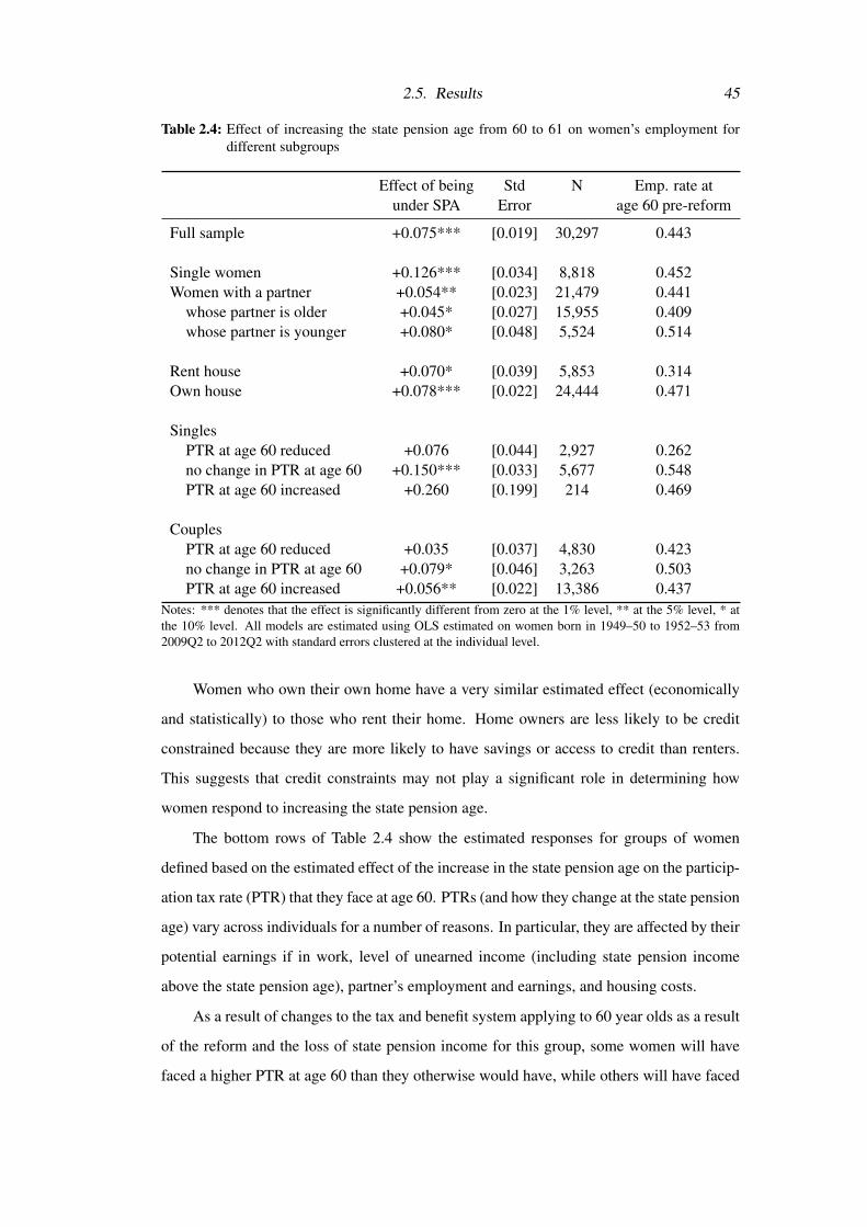
2.5. Results 45
Table 2.4: Effect of increasing the state pension age from 60 to 61 on women’s employment fordifferent subgroups
Effect of being Std N Emp. rate atunder SPA Error age 60 pre-reform
Full sample +0.075*** [0.019] 30,297 0.443
Single women +0.126*** [0.034] 8,818 0.452Women with a partner +0.054** [0.023] 21,479 0.441
whose partner is older +0.045* [0.027] 15,955 0.409whose partner is younger +0.080* [0.048] 5,524 0.514
Rent house +0.070* [0.039] 5,853 0.314Own house +0.078*** [0.022] 24,444 0.471
SinglesPTR at age 60 reduced +0.076 [0.044] 2,927 0.262no change in PTR at age 60 +0.150*** [0.033] 5,677 0.548PTR at age 60 increased +0.260 [0.199] 214 0.469
CouplesPTR at age 60 reduced +0.035 [0.037] 4,830 0.423no change in PTR at age 60 +0.079* [0.046] 3,263 0.503PTR at age 60 increased +0.056** [0.022] 13,386 0.437
Notes: *** denotes that the effect is significantly different from zero at the 1% level, ** at the 5% level, * atthe 10% level. All models are estimated using OLS estimated on women born in 1949–50 to 1952–53 from2009Q2 to 2012Q2 with standard errors clustered at the individual level.
Women who own their own home have a very similar estimated effect (economically
and statistically) to those who rent their home. Home owners are less likely to be credit
constrained because they are more likely to have savings or access to credit than renters.
This suggests that credit constraints may not play a significant role in determining how
women respond to increasing the state pension age.
The bottom rows of Table 2.4 show the estimated responses for groups of women
defined based on the estimated effect of the increase in the state pension age on the particip-
ation tax rate (PTR) that they face at age 60. PTRs (and how they change at the state pension
age) vary across individuals for a number of reasons. In particular, they are affected by their
potential earnings if in work, level of unearned income (including state pension income
above the state pension age), partner’s employment and earnings, and housing costs.
As a result of changes to the tax and benefit system applying to 60 year olds as a result
of the reform and the loss of state pension income for this group, some women will have
faced a higher PTR at age 60 than they otherwise would have, while others will have faced
46 Chapter 2. Increasing the female state pension age
no change or a decrease in their PTR.
It is not trivial to estimate the PTR that our sample of women faces before and after the
state pension age. There are two main complexities in doing so. First, in order to estimate
Equation 2.1, we need to know the PTR faced not only by women who are in work but also
by those who are not working when observed in the survey.22 Second, PTRs depend on a
wide range of circumstances, not all of which are observed in the LFS data – such as housing
costs and state pension entitlement. We therefore have to make use of supplementary data
to estimate the PTRs, following a three-step process to divide our sample into groups that
face a higher/same/lower PTR at age 60 as a result of the increase in the state pension age.
First, we estimate an equation for median earnings of women aged 57 to 59 from
the LFS who are in work, as a function of their education level, their partner’s education
level (or whether they are single),23 housing tenure, and whether they live in London or
the South East. We use the coefficients from this regression to impute ‘potential’ earnings
for all women aged 60 to 64 in the 2008–09 and 2009–10 waves of the Family Resources
Survey (FRS).
The second step is to use the Institute for Fiscal Studies’ (IFS’) tax and benefit mi-
crosimulation model (TAXBEN) to calculate the PTR for each of these women in the FRS
– first assuming that they are aged over the state pension age, and then assuming that they
are aged under the state pension age.
Based on these estimated PTRs, we identify three groups that broadly are likely to face
a higher/same/lower PTR at age 60 as a result of the increase in the state pension age. We
do this separately for singles and couples. The groups we distinguish are based on own
education level, housing tenure, and whether their partner will be aged under or over 65
when they reach age 60. (The last of these is a proxy for partner’s employment status,
which is particularly important in determining out-of-work benefit eligibility.) Importantly,
these are all characteristics that we also observe in the LFS data. Dividing the groups up
requires an element of judgment. Table 2.A.3 in Appendix 2.A describes the mean and
distribution of the estimated change in PTRs among each group. The broad distinguishing
22Not only are the earnings of women who are not in work not observed, but women who work past theage of 60 may be a selected group of women. This means that their earnings may be a poor guide to whatnon-working women could earn were they to work.
23In order to measure education the same way in the LFS and FRS, we use a slightly different measure ofeducation than used elsewhere in this paper. Specifically, we define education groups based on age left full timeeducation, where the ‘low educated’ left at age 15 or below, ‘mid educated’ at age 16 to 18, and ‘high educated’at ages 19 and above.
2.5. Results 47
characteristics of each group are as follows:
• Lower PTR at age 60 as a result of increasing the state pension age
– Singles: mid/low educated renters
– Couples: partner will be aged 65 or over
• No change in PTR at age 60 as a result of increasing the state pension age
– Singles: home owners
– Couples: high educated and partner will be aged under 65
• Higher PTR at age 60 as a result of increasing the state pension age
– Singles: high educated renters
– Couples: mid/low educated and partner will be aged under 65
The final step of the process is to divide our sample of LFS respondents into these same
groups.
If changes in marginal financial incentives were a strong driver of the response to the
policy, we would expect the increase in employment rate to be largest among the group
of women who saw a decrease in their PTR. However, the point estimates are actually
smallest for these groups, although we cannot reject that the coefficients are the same at
normal levels of statistical significance. In other words, we find no evidence that changes in
financial incentives have been an important driver of the responses we observe.
Our calculations suggest that, on average, the increase in the state pension age led to a
small fall in the gain to work (1−PT R) at age 60 of 0.8 percentage points. Therefore, the
large increase in employment that we find implies that the elasticity is substantially larger
and of the opposite sign than credible values of the elasticity estimated previously (see,
for example, Adam and Phillips, 2013). This supports our conclusion that the changes in
financial incentives to work from the increase in the state pension age cannot explain the
large increase in employment seen for women aged 60.
2.5.3 Effect on broader measures of economic status
The effect of increasing the state pension age on employment is important in determining
how raising the state pension age will affect the public finances by generating additional
tax revenues. However, the larger public finance picture and individuals’ welfare will also
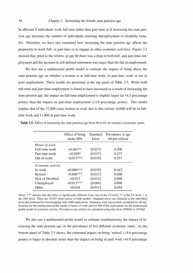
48 Chapter 2. Increasing the female state pension age
be affected if individuals work full-time rather than part-time or if increasing the state pen-
sion age increases the number of individuals claiming unemployment or disability bene-
fits. Therefore, we have also examined how increasing the state pension age affects the
propensity to work full- or part-time or to engage in other economic activities. Figure 2.2
showed that, prior to the reform, at age 60 there was a drop in both full- and part-time em-
ployment and the increase in self-defined retirement was larger than the fall in employment.
We first use a multinomial probit model to estimate the impact of being above the
state pension age on whether a woman is in full-time work, in part-time work or not in
paid employment. These results are presented in the top panel of Table 2.5. While both
full-time and part-time employment is found to have increased as a result of increasing the
state pension age, the impact on full-time employment is slightly larger (at +4.3 percentage
points) than the impact on part-time employment (+3.0 percentage points). This model
implies that of the 27,000 extra women in work due to this reform 16,000 will be in full-
time work and 11,000 in part-time work.
Table 2.5: Effect of increasing the state pension age from 60 to 61 on women’s economic status
Effect of being Standard Prevalence at ageunder SPA Error 60 pre-reform
Hours of workFull time work +0.043** [0.017] 0.206Part time work +0.030* [0.017] 0.237Out of work –0.073*** [0.019] 0.557
Economic activityIn work +0.060*** [0.019] 0.443Retired –0.096*** [0.017] 0.400Sick or Disabled +0.013 [0.012] 0.098Unemployed +0.013*** [0.004] 0.006Other +0.010 [0.011] 0.054
Notes: *** denotes that the effect is significantly different from zero at the 1% level, ** at the 5% level, * atthe 10% level. There are 30,297 observations in both models. Standard errors are clustered at the individuallevel and estimated by bootstrapping with 1000 replications. Estimates were successfully produced for all rep-lications for the multinomial probit model of hours of work and for 990 of the replications for the multinomialprobit model of economic activity. Prevalences pre-reform are calculated using data from 2008Q2 to 2010Q1
We also use a multinomial probit model to estimate simultaneously the impact of in-
creasing the state pension age on the prevalence of five different economic states. As the
bottom panel of Table 2.5 shows, the estimated impact on being ‘retired’ (–9.6 percentage
points) is larger in absolute terms than the impact on being in paid work (+6.0 percentage
2.5. Results 49
points). This model also suggests that there was a significant increase in the proportion of
women reporting being unemployed when the state pension age was increased (+1.3 per-
centage points).24 These estimates imply that a one-year increase in the state pension age led
to an additional 22,000 women in work, 5,000 more women unemployed and 36,000 fewer
women reporting themselves to be retired.25 The increase in prevalence of unemployment
when the state pension age is increased could arise because individuals continue actively
seeking work until they reach state pension age, when they qualify for non-employment
income sources (such as state and private pensions), which do not have the same job search
requirements as working-age out-of-work benefits.26
2.5.4 Effect on the economic status of men
It is also possible to estimate the effect of changing the female state pension age on (male)
partner’s employment. It is unlikely that there is an impact of this change on partners who
are particularly young (because they are likely to work, whether or not their partner is over
the state pension age) or particularly old (because they are likely to be retired whatever the
age of their partner). We therefore restrict our attention to men aged 55 to 69. Results from
estimating probit models of husband’s behaviour are presented in Table 2.6. Full results for
a specification estimated using OLS are reported in Table 2.A.4 in Appendix 2.A.
The impact on men’s employment of increasing the female state pension age is es-
timated to be between 4.2 and 4.5 percentage points, depending on whether a probit or
multinomial probit is used. This effect is consistently significant at the 5% level.27 Our
preferred model, the probit, gives an estimated impact of 4.2 percentage points, which is
consistent with a one-year increase in the female state pension age from 60 to 61 leading to
8,300 more men in paid work. The results suggest that this is mainly due to an increase in
the number of men in full-time work rather than an increase in part-time work. There are24Using labour force participation as the outcome variable in a probit model, we estimate that being under
the state pension age increases labour force participation by 8.2 percentage points, significant at below the 1%level.
25The increase in employment derived from this specification is different from that quoted above because ofthe different methodology used to estimate the answer.
26By February 2012, (the last month for which the Department for Work and Pensions release data onnumber of benefit recipients before the state pension age reaches 61) 1.1% of 60 year olds who were under thestate pension age were on JSA. This figure is consistent with our estimate of a 1.3 percentage points increasein the proportion of women who are unemployed due to the increase in the state pension age. 13.2% of thesame group were claiming disability benefits (incapacity benefit or ESA). Offsetting this to a large extent, therewill have been a reduction in the numbers able to claim pension credit. However, published administrative datasources do not allow us to observe this.
27The point estimate is also robust to using just the first wave of data on each individual (although signi-ficance is reduced due to the lower sample size) and no evidence is found of any impact on male partners’employment rates of a pseudo female state pension age reform introduced two years earlier in 2008.

50 Chapter 2. Increasing the female state pension age
Table 2.6: Effect of increasing partner’s state pension age on men’s economic status
Effect of partner Standardbeing under SPA Error
In work +0.042** [0.022]
Hours of workFull time work +0.037* [0.022]Part time work +0.008 [0.015]Not in work –0.045** [0.022]
Economic activityIn work +0.044** [0.021]Retired –0.026 [0.017]Sick or Disabled –0.024 [0.014]Unemployed +0.003 [0.007]Other +0.004 [0.006]
Notes: ** denotes that the effect is significantly different from zero at the 5% level, * at the 10% level. Thereare 18,776 observations in all models. Estimation run on men aged 55–69 who have partners born between1949–50 to 1952–53 and are observed 2009 Q2 to 2012 Q2. Standard errors are clustered at the individuallevel and estimated by bootstrapping with 1000 replications. Estimates were successfully produced on allreplications of the probit (‘in work’) and multinomial probit model of hours of work and on 911 replicationsfor the multinomial probit of economic activity.
no statistically significant impacts on any other reported economic statuses of men.
As mentioned above, there are two possible reasons that husbands may have changed
their employment behaviour in response to the increase in the female state pension age.
First, there may be complementarities of leisure within couples. Second, couples might
choose to adjust the husband’s employment to compensate for the policy change rather
than the wife working more. The results presented in Table 2.6 are consistent with both of
these explanations. To unpick which of these alternative explanations is most important,
we estimate a multinomial model of the joint work behaviour of couples. The dependent
variable can take four possible values: both members of a couple in paid work, only husband
works, only wife works, neither works. Summary results from estimating this model are
presented in Table 2.7. (The sample and the other covariates included in the regression are
the same as used in the models reported in Table 2.6.)
The right-hand column of Table 2.7 shows the prevalence of different joint working
behaviours among couples (prior to the reform) in which the wife was aged 60 (and the
husband was aged between 55 and 69). This shows that 33.7% of such couples had no one
in work, 11.6% had just the wife working, 25.1% had just the husband working, and 29.7%

2.5. Results 51
Table 2.7: Effect of increasing female state pension age on employment of couples
Effect of wife Standard Prevalence whenbeing under SPA Error wife aged 60
No one in work –0.047** [0.021] 0.337Wife only in work +0.003 [0.017] 0.116Husband only in work –0.010 [0.020] 0.251Both in work +0.054** [0.025] 0.297
Notes: ** denotes that the effect is significantly different from zero at the 5% level. Sample size = 18,766.Estimation run on couples in which the man was aged 55–69 and in which the woman was born in 1949–50 to195253 and are observed 2009Q2 to 2012Q2. Standard errors are clustered at the couple level and estimatedby bootstrapping with 1,000 replications. Estimates were successfully produced on 989 replications of themultinomial probit. Figures for prevalence pre-reform are calculated from data covering 2003–2009.
had both partners working.
Complementarities of leisure within couples would suggest we should see an increase
in the number of two-earner couples and a corresponding decrease in the number of couples
where neither partner is in paid work in response to the reform. The alternative explanation
instead suggests that we would expect to see a decrease in the number of couples where the
husband does not work and an increase in both the number of couples where both partners
work and the number of couples where just the husband works.
The coefficient estimates in Table 2.7 suggest that increasing the female state pension
age reduced the number of couples in which neither partner was in paid work and increased
the number in which both were working, while having no significant effect on the percentage
of couples with just the wife or just the husband working. (If anything, the percentage of
couples in which just the husband worked declined in response to the reform.)
One way of assessing whether this pattern of changes reflects complementary re-
sponses within couples is to compare the change in the prevalence of joint work behaviour
shown in the second column of Table 2.7 to what one would expect to see if the responses
of women and their husbands to this policy (presented in Tables 2.3 and 2.6) were inde-
pendent of one another. If the responses were independent, based on the prevalence of joint
employment behaviour shown in the last column of Table 2.7, we would expect to have seen
a 5.9 percentage point decline in the fraction of couples where no one worked, and an in-
crease in the prevalence of the other groups shown in Table 2.7 by (in order) 1.7 percentage
points, 0.5 percentage points, and 3.7 percentage points. In other words, comparing this to
the second column of Table 2.7, we would instead see a pattern in which much more of the

52 Chapter 2. Increasing the female state pension age
response comes from one or other partner in the couple (rather than both) responding. If
partners’ responses were actually substitutes for one another (that is, negatively correlated),
we would expect to see an even larger increase in the prevalence of one-earner couples and
a smaller increase in the prevalence of two-earner couples. These results suggest that com-
plementarities of leisure within couples dominate any substitution that may have occurred.
2.5.5 Effect on the public finances
Our estimates of the labour supply effect of increasing the female state pension age can
be used to inform a costing of how much an increase in the female state pension age might
strengthen the public finances. In this subsection, we compare a simple costing of a one-year
increase in the female state pension age from 60 to 61 based on no change in labour market
behaviour and a costing that incorporates the increased numbers in paid work implied by
the estimates earlier in this section.
On average, those women aged between 60 and 64 receiving the state pension receive
just over £100 a week in state pension income. Given there are about 370,000 women aged
60, removing this amount of state pension from them would save the Exchequer £2.0 bil-
lion a year. Taking into account a reduction in income tax revenues from this state pension,
reduced spending on means-tested retirement benefits, increased spending on working-age
benefits (JSA and ESA), an increase in payroll taxes from those women aged 60 in paid
work, and a fall in indirect taxes from the fall in net household incomes, the overall estim-
ated strengthening in the public finances falls slightly to £1.9 billion a year.28
However, this figure does not allow for any additional tax revenue from individuals
increasing their employment and earnings in response to the increase in the state pension
age. Controlling for age, cohort, time and background variables in the same functional
form as in Section 2.4, we use OLS to estimate the impact of increasing the female state
pension age on the weekly earnings of 60-year-old women (those not in paid work are
included, having earnings of zero) and find that increasing the state pension age increases
the earnings of 60-year-old women by an average of £22.36 a week and that of their partners
by an average of £24.02 a week. Under the assumption that this comes entirely from those
28These figures are all based on calculations using the Department for Work and Pensions tabulation tool(http://research.dwp.gov.uk/asd/index.php?page=tabtool). The increases in JSA andESA spending (of £36 million and £12 million) are taken directly from information on the amounts now re-ceived by women aged 60. We assume that women only have a high enough income to pay income tax on theirstate pension if they have other income from employment. NICs revenues estimated using the LFS. Indirecttaxes assumed to fall by 10% of the fall in net incomes.
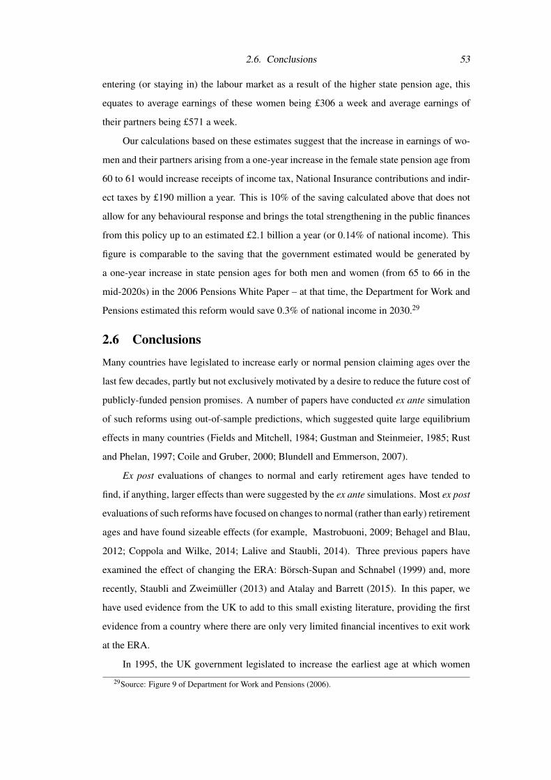
2.6. Conclusions 53
entering (or staying in) the labour market as a result of the higher state pension age, this
equates to average earnings of these women being £306 a week and average earnings of
their partners being £571 a week.
Our calculations based on these estimates suggest that the increase in earnings of wo-
men and their partners arising from a one-year increase in the female state pension age from
60 to 61 would increase receipts of income tax, National Insurance contributions and indir-
ect taxes by £190 million a year. This is 10% of the saving calculated above that does not
allow for any behavioural response and brings the total strengthening in the public finances
from this policy up to an estimated £2.1 billion a year (or 0.14% of national income). This
figure is comparable to the saving that the government estimated would be generated by
a one-year increase in state pension ages for both men and women (from 65 to 66 in the
mid-2020s) in the 2006 Pensions White Paper – at that time, the Department for Work and
Pensions estimated this reform would save 0.3% of national income in 2030.29
2.6 Conclusions
Many countries have legislated to increase early or normal pension claiming ages over the
last few decades, partly but not exclusively motivated by a desire to reduce the future cost of
publicly-funded pension promises. A number of papers have conducted ex ante simulation
of such reforms using out-of-sample predictions, which suggested quite large equilibrium
effects in many countries (Fields and Mitchell, 1984; Gustman and Steinmeier, 1985; Rust
and Phelan, 1997; Coile and Gruber, 2000; Blundell and Emmerson, 2007).
Ex post evaluations of changes to normal and early retirement ages have tended to
find, if anything, larger effects than were suggested by the ex ante simulations. Most ex post
evaluations of such reforms have focused on changes to normal (rather than early) retirement
ages and have found sizeable effects (for example, Mastrobuoni, 2009; Behagel and Blau,
2012; Coppola and Wilke, 2014; Lalive and Staubli, 2014). Three previous papers have
examined the effect of changing the ERA: Borsch-Supan and Schnabel (1999) and, more
recently, Staubli and Zweimuller (2013) and Atalay and Barrett (2015). In this paper, we
have used evidence from the UK to add to this small existing literature, providing the first
evidence from a country where there are only very limited financial incentives to exit work
at the ERA.
In 1995, the UK government legislated to increase the earliest age at which women
29Source: Figure 9 of Department for Work and Pensions (2006).
54 Chapter 2. Increasing the female state pension age
could claim a state pension from 60 to 65 between April 2010 and March 2020. This paper is
the first to examine (ex post) the impact of this policy on women’s economic activity at older
ages and that of their partners, using data covering the period up to June 2012. Our results,
which allow for a flexible specification of cohort effects, suggest that employment rates did
increase significantly as a result of the change in state pension age – by 7.3 percentage points
using our preferred specification. We find statistically significant rises in both full-time and
part-time female employment as a result of the reform.
In addition to the impact on employment rates, we find the policy has also led to a
1.3 percentage point increase in the fraction of women who are unemployed and actively
seeking work at age 60. These increases in employment and unemployment are offset by
a reduction in the proportion reporting themselves to be retired. No significant differences
were found in other economic activities (sick/disabled and looking after home/other).
Subgroup analysis provides some tentative evidence on which mechanisms may be
important in explaining the changes in behaviour that we observe. There is no signific-
ant difference in the response among owner-occupiers and renters, which we interpret as
suggestive evidence that credit constraints may not be the primary driver. We also find no
evidence that the increase in employment is largest among those who are likely to have
faced the largest decrease in participation tax rates. This is suggestive that marginal finan-
cial incentives are also not a major explanatory factor. In addition, the cohort fixed effects
included in our model control for differences in state pension wealth across cohorts that are
a direct result of the increase in the state pension age. Therefore, unless wealth effects affect
behaviour in a non-linear way that is not allowed for in our model, we can also rule out that
these are the major driving force of the response we see.
Overall, we find a large impact of the increase in the state pension age on female labour
market behaviour despite the UK system having no earnings test for receipt of state pension
income. Together with the suggestive evidence on the importance (or lack thereof) of credit
constrains, marginal financial incentives, and wealth effects in explaining the response we
see, this suggests that the role of the state pension age in providing a signal about the
appropriate retirement age may be an important reason why increasing the state pension
age feeds through into such a sizeable effect on labour force participation.
We also find a significant effect of the policy on employment rates of affected women’s
partners, with men’s employment rates being found to increase by 4.2 percentage points as
2.6. Conclusions 55
a result of their female partners’ state pension age increasing. This suggests that the policy
of increasing the female state pension age has had a knock-on effect on men’s employment
rates.
In principle this knock-on effect on partners could reflect either complementarities in
leisure or the fact that couples who make joint financial decisions decide to cushion the
impact of the woman’s higher state pension age through a combination of both the man
and the woman working for longer, rather than adjusting solely on the female labour supply
margin. Evidence from looking at the employment of both members of the couple suggests
that the increase in the female state pension age has led to an increase in two-earner couples,
a decrease in the fraction of couples where neither is in paid work and no significant change
in the fraction of couples where only the husband or only the wife is in paid work. We
interpret this as evidence that complementarities of leisure within couples dominates any
tendency for couples to use alternative margins (male and female labour supply) to respond
to the policy change.
Taken together these results suggest that the increase in the female state pension age
will have strengthened the UK’s public finances not only by reducing payments to pension-
ers but also by increasing tax revenues from earned income among older women and their
partners. Our estimates suggest that a one-year increase in the female state pension age
from 60 to 61 led to 27,000 more women, and 8,300 more men, being in paid work. The
overall saving to the Exchequer (both from changes in spending and changes in tax rev-
enues) from this one-year increase in the female state pension age is estimated to be £2.1
billion a year after taking the resulting increase in earnings into account. This is 10% higher
than an estimate that does not take into account any change in labour market behaviour.
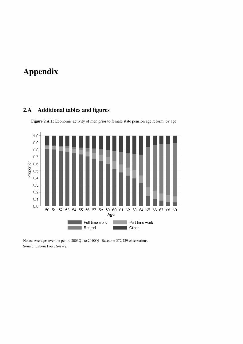
Appendix
2.A Additional tables and figures
Figure 2.A.1: Economic activity of men prior to female state pension age reform, by age
Notes: Averages over the period 2003Q1 to 2010Q1. Based on 372,229 observations.
Source: Labour Force Survey.

2.A. Additional tables and figures 57
Figure 2.A.2: Employment rates of older men, 2003–2012
Notes: Based on 160,114 observations.
Source: Labour Force Survey, 2003 to 2012.

58 Chapter 2. Increasing the female state pension age
Tabl
e2.
A.1
:Num
bero
fwom
enob
serv
edab
ove
and
belo
wst
ate
pens
ion
age
Bir
thA
gein
year
and
quar
ters
coho
rt58
Q1
58Q
258
Q3
58Q
459
Q1
59Q
259
Q3
59Q
460
Q1
60Q
260
Q3
60Q
461
Q1
61Q
261
Q3
61Q
4
1949
Q2
7316
515
915
815
516
816
616
413
719
49Q
373
154
149
139
134
155
137
128
125
147
1949
Q4
7615
315
717
215
716
215
014
414
113
416
119
50Q
192
171
186
174
159
169
154
151
129
138
129
147
1950
Q2
8018
117
917
517
817
116
915
815
514
616
315
113
519
50Q
375
173
170
159
148
142
121
128
119
138
147
163
146
8419
50Q
460
154
152
149
137
134
120
120
115
131
140
157
134
7819
51Q
172
145
137
137
139
138
121
123
123
126
150
152
154
7619
51Q
216
116
718
918
417
715
715
513
213
313
814
914
875
1951
Q3
139
129
133
131
121
125
110
112
128
144
141
8219
51Q
413
614
215
012
911
712
513
013
413
712
757
1952
Q1
158
153
137
151
129
122
142
150
145
8219
52Q
214
913
814
413
413
614
217
014
184
1952
Q3
141
130
114
126
137
142
126
6319
52Q
414
914
112
613
013
213
369
1953
Q1
117
132
129
144
132
84
Not
es:
Dar
ksh
aded
cells
indi
cate
wom
enw
hoar
eal
love
rthe
irst
ate
pens
ion
age.
Lig
htsh
aded
cells
indi
cate
com
bina
tions
ofag
ean
dco
hort
whe
reso
me
wom
enar
eab
ove
and
som
ew
omen
are
belo
wth
est
ate
pens
ion
age.
Em
pty
cells
exis
tbec
ause
coho
rts
are
noto
bser
ved
atal
lage
sin
the
peri
od20
09Q
2to
2012
Q2
whi
chw
eus
ein
our
estim
atio
n.N
umbe
rof
wom
enre
fers
tonu
mbe
rofo
bser
vatio
nsin
the
LFS
with
outd
ata
prob
lem
s,an
dw
hich
are
ther
efor
eus
edin
estim
atio
nof
impa
ctof
bein
gag
edun
dert
hest
ate
pens
ion
age.

2.A. Additional tables and figures 59
Table 2.A.2: Effect of state pension age on female employment: OLS regression
Effect on female Standardemployment error
Under SPA 0.075*** [0.019]Cohabiting 0.063*** [0.024]Single –0.065** [0.030]Widowed –0.047* [0.028]Divorced/separated 0.019 [0.025]Other HE –0.069*** [0.018]A level or equivalent –0.034* [0.019]O level or equivalent –0.065*** [0.017]Other –0.094*** [0.019]No qualifications –0.245*** [0.018]Non-white –0.095*** [0.023]Rents house –0.172*** [0.013]Partner’s age (years and quarters) –0.015 [0.013]Partner’s age squared 0.000 [0.000]Partner’s age: 60–64 –0.040** [0.017]Partner’s age: 65–69 –0.094*** [0.029]Partner’s age: 70+ –0.073 [0.057]Partner’s education: other HE 0.069*** [0.023]Partner’s education: A level 0.070*** [0.018]Partner’s education: O level 0.076*** [0.023]Partner’s education: other 0.091*** [0.022]Partner’s education: no qualifications 0.058*** [0.022]
Notes: *** denotes that the effect is significantly different from zero at the 1% level, ** at the 5% level, * at the10% level. Estimated by OLS with standard errors clustered at the individual level. This regression model useswomen born in 1949–50 to 1952–53 from 2009Q2 to 2012Q2. Nineteen geographical area dummy variables,12 year and quarter dummy variables, dummies for age in years and quarters, dummies for financial year ofbirth, and a constant also included in the model. Effects estimated relative to baseline of cohort 1949–50, age60Q1, married, white, owns house, with a degree, and with a partner with a degree. Number of observations:30,297.
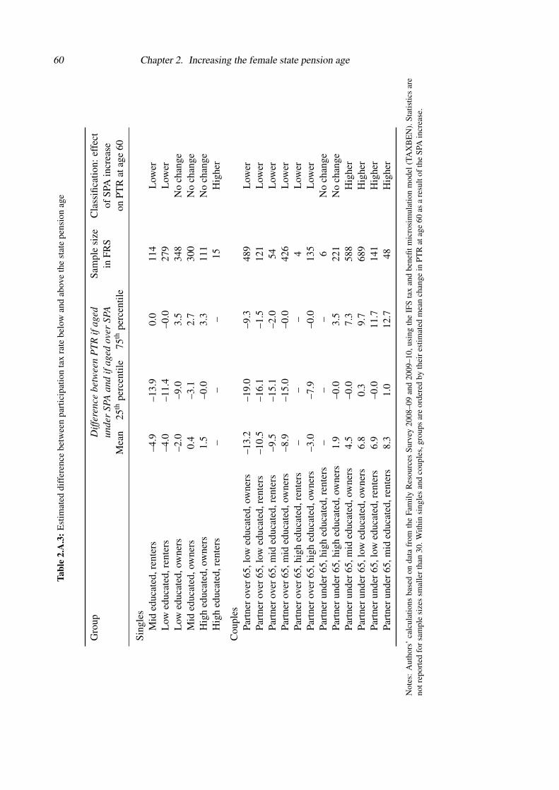
60 Chapter 2. Increasing the female state pension ageTa
ble
2.A
.3:E
stim
ated
diff
eren
cebe
twee
npa
rtic
ipat
ion
tax
rate
belo
wan
dab
ove
the
stat
epe
nsio
nag
e
Gro
upD
iffer
ence
betw
een
PTR
ifag
edSa
mpl
esi
zeC
lass
ifica
tion:
effe
ctun
der
SPA
and
ifag
edov
erSP
Ain
FRS
ofSP
Ain
crea
seM
ean
25th
perc
entil
e75
thpe
rcen
tile
onPT
Rat
age
60
Sing
les
Mid
educ
ated
,ren
ters
–4.9
–13.
90.
011
4L
ower
Low
educ
ated
,ren
ters
–4.0
–11.
4–0
.027
9L
ower
Low
educ
ated
,ow
ners
–2.0
–9.0
3.5
348
No
chan
geM
ided
ucat
ed,o
wne
rs0.
4–3
.12.
730
0N
och
ange
Hig
hed
ucat
ed,o
wne
rs1.
5–0
.03.
311
1N
och
ange
Hig
hed
ucat
ed,r
ente
rs–
––
15H
ighe
r
Cou
ples
Part
nero
ver6
5,lo
wed
ucat
ed,o
wne
rs–1
3.2
–19.
0–9
.348
9L
ower
Part
nero
ver6
5,lo
wed
ucat
ed,r
ente
rs–1
0.5
–16.
1–1
.512
1L
ower
Part
nero
ver6
5,m
ided
ucat
ed,r
ente
rs–9
.5–1
5.1
–2.0
54L
ower
Part
nero
ver6
5,m
ided
ucat
ed,o
wne
rs–8
.9–1
5.0
–0.0
426
Low
erPa
rtne
rove
r65,
high
educ
ated
,ren
ters
––
–4
Low
erPa
rtne
rove
r65,
high
educ
ated
,ow
ners
–3.0
–7.9
–0.0
135
Low
erPa
rtne
rund
er65
,hig
hed
ucat
ed,r
ente
rs–
––
6N
och
ange
Part
neru
nder
65,h
igh
educ
ated
,ow
ners
1.9
–0.0
3.5
221
No
chan
gePa
rtne
rund
er65
,mid
educ
ated
,ow
ners
4.5
–0.0
7.3
588
Hig
her
Part
neru
nder
65,l
owed
ucat
ed,o
wne
rs6.
80.
39.
768
9H
ighe
rPa
rtne
rund
er65
,low
educ
ated
,ren
ters
6.9
–0.0
11.7
141
Hig
her
Part
neru
nder
65,m
ided
ucat
ed,r
ente
rs8.
31.
012
.748
Hig
her
Not
es:
Aut
hors
’ca
lcul
atio
nsba
sed
onda
tafr
omth
eFa
mily
Res
ourc
esSu
rvey
2008
–09
and
2009
–10,
usin
gth
eIF
Sta
xan
dbe
nefit
mic
rosi
mul
atio
nm
odel
(TA
XB
EN
).St
atis
tics
are
notr
epor
ted
fors
ampl
esi
zes
smal
lert
han
30.W
ithin
sing
les
and
coup
les,
grou
psar
eor
dere
dby
thei
rest
imat
edm
ean
chan
gein
PTR
atag
e60
asa
resu
ltof
the
SPA
incr
ease
.

2.A. Additional tables and figures 61
Table 2.A.4: Effect of female state pension age on male employment: OLS regression
Effect on male Standardemployment error
Partner under SPA 0.044* [0.023]Own age –0.086 [0.076]Own age squared 0.000 [0.001]Is 65 or older –0.126*** [0.029]Is over female SPA –0.016 [0.021]Cohabiting 0.019 [0.030]Other HE –0.017 [0.024]A level or equivalent –0.019 [0.019]O level or equivalent –0.033 [0.024]Other 0.031 [0.023]No qualifications –0.076*** [0.024]Non-white –0.117*** [0.034]Rents house –0.160*** [0.020]Partner’s education: other HE –0.001 [0.023]Partner’s education: A level or equivalent 0.040* [0.024]Partner’s education: O level or equivalent 0.012 [0.022]Partner’s education: other 0.028 [0.024]Partner’s education: no qualifications –0.011 [0.023]
Notes: *** denotes that the effect is significantly different from zero at the 1% level, * at the 10% level.Estimated by OLS with standard errors clustered at the individual level. Regression model using men aged55–69 with female partners born in 1949–50 to 1952–53 from 2009Q2 to 2012Q2. Nineteen geographicalarea dummy variables, 12 year and quarter dummy variables, dummies for partner’s age in years and quarters,dummies for partner’s financial year of birth, and constant also included in the model. Effects estimated relativeto baseline of partner’s cohort 1949–50, partner’s age 60Q1, married, white, owns house, with a degree, andwith a partner with a degree. Number of observations: 18,774.

62 Chapter 2. Increasing the female state pension age
2.B Effect of increasing the state pension age on employment
rates before age 60
Raising the state pension age from 60 to 61 could potentially have an impact on women’s
labour supply and retirement before age 60. Our model, as laid out in Equation 2.1, rules
out any labour supply impact of the increase in the state pension age prior to age 60. Any
response before age 60 will be subsumed within the cohort fixed effects included in the
model and, as a result, the estimates we produce for the impact on employment above the
old state pension age are over and above any increase that occurred at earlier ages. However,
using a different methodology (that used by Mastrobuoni, 2009), we can estimate whether
there has been any change in labour supply at other ages. In particular, we estimate whether
there has been any change in employment rates of women between the ages of 55 and 59.
We first estimate the average retirement rates for each cohort of women at each age between
55 and 59 using Equation 2.2.
yi =59Q4
∑a=55Q1
1(Ai = a)[αa + ∑
c 6=1949−50βa,c1(Ci = c)
]+ γ
′Xi + εi (2.2)
Equation 2.2, which we estimate using OLS, includes a cohort-specific age (in year
and quarter) effect βa,c. The dependent variable is an indicator of not being in work (i.e.
retirement). The vector of control variables (Xi) contains an indicator of owning a house, a
measure of highest educational qualification, an indicator of being married, regional dum-
mies, and the regional unemployment rate of women aged 45 to 54 in the quarter of observa-
tion. The last of these variables is included in order to pick up any potentially confounding
macroeconomic trends. We estimate this model for all women born in the financial years
1945–46 to 1952–53. Using the results of this estimation, we can calculate the change in the
average retirement age between cohorts, using women born in the 1949–50 financial year
(i.e. the latest cohort to have a state pension age of 60) as the comparison group. In other
words, βa,1949−50 = 0 ∀a. The change in average retirement age (that manifests between
ages 55 and 59) can be calculated using Equation 2.3.
∆c =59Q4
∑a=55Q1
1(Ai = a)[αa +βa,c1(Ci = c)
]−
59Q4
∑a=55Q1
1(Ai = a)αa
= β55Q1,c +β55Q2,c + · · ·+β59Q4,c (2.3)
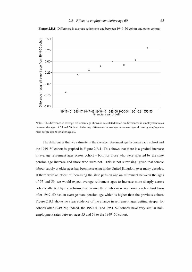
2.B. Effect on employment before age 60 63
Figure 2.B.1: Difference in average retirement age between 1949–50 cohort and other cohorts
Notes: The difference in average retirement age shown is calculated based on differences in employment rates
between the ages of 55 and 59, it excludes any differences in average retirement ages driven by employment
rates before age 55 or after age 59.
The differences that we estimate in the average retirement age between each cohort and
the 1949–50 cohort is graphed in Figure 2.B.1. This shows that there is a gradual increase
in average retirement ages across cohort – both for those who were affected by the state
pension age increase and those who were not. This is not surprising, given that female
labour supply at older ages has been increasing in the United Kingdom over many decades.
If there were an effect of increasing the state pension age on retirement between the ages
of 55 and 59, we would expect average retirement ages to increase more sharply across
cohorts affected by the reforms than across those who were not, since each cohort born
after 1949–50 has an average state pension age which is higher than the previous cohort.
Figure 2.B.1 shows no clear evidence of the change in retirement ages getting steeper for
cohorts after 1949–50; indeed, the 1950–51 and 1951–52 cohorts have very similar non-
employment rates between ages 55 and 59 to the 1949–50 cohort.


Chapter 3
Can dynamic financial incentives explain
older workers’ labour supply?
3.1 Introduction1
Developed countries face rapidly ageing populations, as longer life expectancies and de-
clining fertility serve to increase the average age of their populations. As people live for
longer, they are faced with a choice between three options: consuming less while work-
ing in order to support an increasingly lengthy retirement, consuming less each year while
retired, and/or working for longer.2 There has been concern among policymakers that too
much of the adjustment will happen on the second margin (perhaps putting pressure on the
government to divert a greater share of tax revenues to support older people), which has led
to considerable interest in what determines the third margin – working for longer – and how
policy might encourage this.
Over the last two decades, increases in life expectancy have been accompanied by
rising employment rates among older people in many developed countries (Wise, 2015).
An interesting question is to what extent (changes in) financial incentives to retire have
affected individuals’ labour force participation. A lot of attention has been paid in the
economic literature and also among policymakers to how individuals respond to dynamic
financial incentives towards the end of their working lives. But to what extent can such fin-
1This chapter is based on earlier joint work with James Banks and Carl Emmerson, which has been pub-lished as Banks, Emmerson, and Tetlow (2007b, 2015). I am grateful to Richard Blundell, Andrew Chesher,Richard Disney, Eric French and Guy Laroque for comments and to Rowena Crawford for comments and forhelping with the calculation of pension entitlements in ELSA waves 2–5. This paper has also benefited fromhelpful discussions with participants in the NBER’s International Social Security project and from commentsreceived from seminar participants at University College London.
2Individuals could end up consuming less while working either voluntarily or as a result of being requiredto pay higher taxes in order to finance state-provided benefits for retirees.

66 Chapter 3. Dynamic financial incentives and labour supply
ancial incentives explain individual behaviour, particularly in a world where – increasingly
– incentives to draw pension income are being decoupled from decisions about labour force
participation?
In this paper, I use detailed information from an English household panel survey to
estimate how much older men and women’s retirement decisions have responded to the
dynamic financial incentives that they face from public and private pensions and the tax
and benefit system in the United Kingdom (UK) over the last decade. I examine whether
responses differ between those in better and worse health and whether responsiveness to
financial incentives has changed over time. Using my estimation results, I simulate the effect
of a reform that increases the state pension age by one year. This illustrative reform has the
effect of delaying the point at which individuals are eligible to receive their state pension
and increasing the incentive for people to continue working in order to accrue additional
state pension entitlements.
When individuals decide whether or not to continue working at older ages, they must
solve an inherently forward-looking, dynamic problem. Many public and private pension
schemes have highly non-linear patterns of accrual with age. Therefore, the relevant ques-
tion for an older individual when deciding whether or not to work next year is not simply
whether the additional benefit obtained in that year sufficiently outweighs the cost, but rather
whether the future ‘path’ that it would put her on would be more attractive than the other
paths that would remain open to her if she chose instead to keep working. Two main types
of approach have been taken in the literature to estimating this forward-looking individual
retirement decision.
One branch of the literature has constructed and estimated stochastic dynamic pro-
gramming models – explicitly modelling individuals’ decision rules. Early contributions
to this literature include Rust (1989), Berkovec and Stern (1991) and Daula and Moffitt
(1992). Since then, rapidly improving computing power has allowed researchers to estim-
ate increasingly complex models. More recent contributions to this literature include French
(2005), Gustman and Steinmeier (2005) and Bound, Stinebrickner, and Waidmann (2010).
These papers fully specify the decision problem and uncertainty facing the individual and
assume that – in deciding which options to choose – the individual solves this dynamic
programming problem.
A second branch of the literature has instead followed the ‘option value’ approach

3.1. Introduction 67
suggested by Stock and Wise (1990). The option value model is similar in spirit to the full
dynamic programming approach but involves a less complex decision rule. A number of
papers have adopted a variant of this approach. For example, Coile and Gruber (2007) look
at retirement in the United States, Blundell, Meghir, and Smith (2004) examine retirement
of older men in the UK, Belloni and Alessie (2009, 2013) examine retirement of men and
women in Italy, and the papers included in Gruber and Wise (2004) apply this model to a
further nine developed countries.
Neither of these approaches is a perfectly ‘correct’ approximation to underyling indi-
vidual behaviour, each imposes some assumptions about how individuals make decisions.
Dynamic programming models have the advantage of being able to incorporate clearly spe-
cified dynamics and decision rules, and improved computer power in recent years has al-
lowed researchers to incorporate increasing realism into such models. However, such mod-
els also assume that individuals have the capacity to solve these complex decision rules
when making their choices.
The option value model, in contrast, is more restrictive in how it allows for dynamics.
However, because of its simpler structure, it can incorporate some features of reality that are
more difficult to incorporate in dynamic programming models – for example, few dynamic
programming models incorporate separate defined benefit and defined contribution pension
assets, despite the fact that these assets have very different characteristics.3 Furthermore, as
the option value model is computationally less complex, it assumes less numerical ability
on the part of individuals, which may be more realistic.
It is not clear ex ante therefore which type of model will be a better approximation to
individual behaviour. This is an empirical question. Lumsdaine, Stock, and Wise (1992),
for example, find that the option value model and two alternative dynamic programming
models performed similarly well in predicting how individuals would respond to changes
in the incentives facing members of a particular firm’s pension plan in the early 1980s.
Daula and Moffitt (1992) find that a model akin to the option value model fits their data
on exits from the military slightly better than their dynamic programming model, though
they argue that simulated behaviour from their dynamic programming model is qualitatively
more plausible than that implied by the option value-type model.
Since the option value model evaluates the maximum of the expected values while
3Blau (2015) is one very recent exception.

68 Chapter 3. Dynamic financial incentives and labour supply
the dynamic programming approach evaluates the expected value of the maximum, the op-
tion value model will tend to understate the value of postponing retirement if the dynamic
programming rule is actually correct. This understatement will be greater if future uncer-
tainty about the value of retirement is large relative to the change in the expected value from
delaying retirement. Dynamic programming models typically make some (unverifiable) as-
sumption about how much the future is uncertain and how much it is predictable, and thus
how large uncertainty is relative to expected changes.
In this paper I estimate a variant of the option value model proposed by Stock and Wise
(1990) to examine the response to financial incentives among older men and women in Eng-
land between 2002 and 2012. I am not able directly to test whether a dynamic programming
model would perform better than the option value model I present here. However, I discuss
at the end of this chapter how a dynamic programming model might fare relative to my
option value approach.
No similar estimation of the importance of dynamic financial incentives for the retire-
ment decisions of older people in England has been done since Blundell, Meghir, and Smith
(2002, 2004).4 They examined the behaviour of older men in the early 1990s. The current
paper is a considerable advance on what Blundell, Meghir, and Smith (2002) were able to
do. In particular, I add to what they did in four main ways. First, I use more recent data.
This is interesting not only because the structure of the pension, tax and benefit systems has
changed quite significantly over recent decades but also because overall employment rates
of older people have changed, suggesting that the dynamics of labour force participation
may be different now. Employment rates of older men have been increasing steadily since
the mid-1990s, having fallen dramatically between the late 1960s and early 1990s.5
Second, the household survey data I use contains much richer data on pension rights
and scheme rules than was available to Blundell, Meghir, and Smith (2002). I am, therefore,
able to model much more accurately individuals’ incentives. Third, I examine the retirement
behaviour of women as well as men. To my knowledge no previous work has examined the
responsiveness of older women in England to financial incentives.6 This is a significant
omission since women in their fifties are now as likely as men of the same age to be in
4The only exceptions are earlier versions of my own work, of which this paper is the culmination (Banks,Emmerson, and Tetlow, 2007b, 2015).
5For a description of how employment rates evolved from the late 1960s to the 2010s and some possibleexplanations for these trends, see, for example, Chandler and Tetlow (2014b).
6Again, the exceptions are earlier versions of my own work (Banks, Emmerson, and Tetlow, 2007b, 2015).

3.1. Introduction 69
employment (although they are somewhat less likely to be in self-employment). This means
that, to understand how overall labour supply of older people might respond to financial
incentives, we need to understand how both men and women will react to changes in these
incentives. Fourth, I model more precisely eligibility for non-pension out of work benefits,
which affect the option value particularly for low wage individuals for whom means-tested
out of work benefits can provide a relatively high replacement rate.
The UK is an interesting case to study as, unlike many other countries, the pen-
sion schemes to which individuals belong differ markedly from one another (as pensions
provided by individual employers, and not just public pension schemes, play a major role in
providing retirement income) and there have been a series of reforms over the last few dec-
ades that have affected the pension wealth and incentives faced by different groups. There
is therefore considerable exogenous variation in pension wealth and incentives among older
workers in the UK, which facilitates the identification of the model presented here.
The UK is also an interesting case because, while there are financial incentives to
draw pensions at particular ages, the link between this and exiting work has become (in
theory) increasingly weak, as a result of a series of reforms over the last decade. It is
therefore interesting to examine whether individuals’ labour supply is responsive to the
pension-drawing incentives, even in an environment where this link is, in principle, weak.
Exploiting variation across individuals in the financial incentives they face, I find that
on average older workers’ retirement decisions respond in an economically and statistically
significant way to the financial incentives captured by the option value. I find no evidence
that the responsiveness of retirement decisions to financial incentives has changed over
the time period I examine, despite reforms that have (in theory) weakened the relationship
between financial incentives to draw a pension and incentives to leave work.
Despite the fact that financial incentives significantly affect the timing of retirement,
they cannot explain the large spikes seen in retirement at specific ages – notably ages 60
and 65. This suggests that other factors – in addition to financial incentives – are important
for determining the timing of retirement. Understanding more about these factors should be
a priority for future work.
Section 3.2 starts by describing the institutional arrangements in the UK and high-
lights those which generate exogenous variation in financial incentives, which is required
to identify the model. Section 3.3 then describes how I model the financial incentives that

70 Chapter 3. Dynamic financial incentives and labour supply
individuals face when making their retirement decisions and my empirical specification.
Section 3.4 describes the data used and presents descriptive statistics, with estimation res-
ults presented in Section 3.5. In order to illustrate the implications of my results, in Section
3.6 I use the estimated coefficients to simulate what the effect would be of increasing the
state pension age by one year. This is similar to the reform to the female state pension age
that is currently being implemented in the UK, which was evaluated in Chapter 2; I discuss
how my simulation results compare to those findings. Section 3.7 concludes.
3.2 Institutional details
In the UK there are two main sources of retirement income for older people – state pensions
and private pensions. However, individuals’ income also depends on the tax and benefit
system. In this section I describe the main non-earned income sources that are available
to older people and the relevant features of the direct personal tax system that affect the
attractiveness of retiring at different future dates.
3.2.1 State pensions
The UK state pension has two parts: the basic state pension (BSP) and the second-tier
state pension.7 People can accrue partial or full entitlement to each of these components
depending on their employment and earnings history and other behaviour during working
life. A full BSP in 2015–16 is worth £115.95 per week (or around 18% of average weekly
earnings).8 This amount is currently increased each year in line with the greatest of price
inflation, average earnings growth and 2.5%.
People receive the full amount of BSP if they have at least 30 years of contributions
or credits.9 The contribution conditions are broad, meaning that most men and women now
reaching the state pension age qualify for the full award. Contributions include (among
other things) being employed or self-employed, caring for children or disabled adults, and
receiving unemployment or disability-related benefits.
The second-tier pension, currently known as the state second pension (S2P), is re-
lated to earnings across the whole of working life (from 1978 onwards). Enhancements
7For full details of the UK state pension system and how the rules have changed over time, see Bozio,Crawford, and Tetlow (2010).
8See Table 2.1a of Department for Work and Pensions (2014).9The pension rules described here relate to the pension system in place prior to the 2013 Pensions Act.
This is because the data I use in estimating my model were collected between spring 2002 and summer 2013,before Pensions Act 2013 took effect. Pensions Act 2013 legislated for significant reforms but these will onlyaffect those reaching state pension age from April 2016 onwards.

3.2. Institutional details 71
are also awarded for periods since April 2002 spent out of work due to some formal caring
responsibilities. The second-tier pension scheme replaces 20% of earnings within a certain
band. The maximum total weekly benefit that could have been received from the second-tier
pension by someone reaching the state pension age in 2012–13 was £161.94.10 However,
historically, the majority of employees have opted out of this second-tier pension and in-
stead built up a private pension (of approximately equal value) in return for paying a lower
rate of the payroll tax (known as National Insurance Contributions, or NICs). Therefore,
the majority of pensioners receive far less than this maximum amount.
The state pension is payable from the state pension age onwards. It cannot be received
before this age but recipients can choose to defer receipt of their state pension. If they do
so, they receive an uplift of 10.4% per year that they defer.11 Between 1948 and April 2010,
the state pension age was 65 for men and 60 for women. Since April 2010 the state pension
age for women has been rising and the intention is that by 2018 it will be equalised at age
65 for both men and women. There is no ‘earnings test’ for receipt of the state pension: that
is, the amount received is not reduced if the individual also has earned income (although
receipt of state pension may result in an increase in the marginal tax rate on earned income,
discussed below).
During the period covered by the data I use here, most individuals faced some incentive
to continue ‘contributing’ to the system until they reached the state pension age, because
additional contributions will have increased the amount of state pension income they would
receive. However, once an individual has accrued 30 years of BSP entitlement, the marginal
accrual of additional pension declines. Furthermore, individuals can potentially accrue extra
state pension entitlement not only through paid work but also through various non-paid work
activities.
Since the same amount of state pension can be received from the state pension age
regardless of whether the individual has actually left the labour market or not, there is no
financial incentive from the state pension system actually to leave the labour market at this
point – aside from the fact that receiving state pension benefits may ease credit constraints
or affect marginal tax rates for some people at this point. Despite this, the state pension age
10See page 8 of Pensions Policy Institute (2013).11In practice, very few people exercise this option. For example, among ELSA respondents aged over the
state pension age but less than age 75 in 2008–09, just 4.3% reported having deferred receipt of their statepension for any period. Nonetheless I allow for it in the calculation of the option values.

72 Chapter 3. Dynamic financial incentives and labour supply
is the single most common age for men and women to withdraw from the labour market.12
Previous legislation (passed in 1975, 1986, 1995 and 2000) has changed the generosity
of the state pension significantly, with the changes varying by individuals’ date of birth, sex,
history of caring responsibilities and earnings. The 1975 and 2000 reforms significantly in-
creased the average generosity of the state pension system, while the 1986 and 1995 reforms
significantly reduced it. These changes have generated differences in the lifetime wealth of
individuals born at different points in time and have also induced differences in the rate at
which additional state pension rights accrue at the margin for different cohorts, meaning
that retirement incentives differ across cohorts. This is one of the sources of exogenous
variation that I exploit to identify my model.
The state pension system has become increasingly generous over time to low earners
and some groups not in paid work, but the generosity of the system to higher earners peaked
among those reaching state pension age in 2000.13 My data cover cohorts born between
1933 and 1958, who will reach state pension age between 1993 and 2024 and have all faced
a variety of state pension rules.
3.2.2 Private pensions
Private pensions are more important for some people in the UK than state pensions in
providing incentives to stay in or leave paid work. Private pensions have always played
a significant part in retirement income provision in the UK, being probably both an ex-
planation for and a consequence of the low level of state pension provision. In 2011–12,
60% of employees aged between 55 and 59 had some form of private pension coverage.14
For some people, part of this private pension provision will be a direct substitute for state
pension provision since, as mentioned above, many individuals choose to opt out of the
second-tier state pension and instead save in a private pension. This has been possible for
members of defined benefit (DB) schemes since 1978 and was also possible for defined
contribution (DC) scheme members between 1987 and 2012. But many employees also
have additional private pension saving – either in DB or DC pensions – above the minimum
required second-tier pension provision.
12As Figures 2.2 and 2.A.1 in Chapter 2 show, the employment rates of men and women drop by around14 percentage points at their respective state pension ages. These are larger falls than seen between any otherconsecutive ages but nonetheless the majority of people exit work at other ages.
13For a description of the generosity of the state pension system to high and low earners born in differentyears, see Crawford, Keynes, and Tetlow (2013).
14See Chapter 6 of Department for Work and Pensions (2013).

3.2. Institutional details 73
Different types of private pension arrangements can and do lead to significant differ-
ences in the financial incentives that those in paid work face to start drawing their pension
at particular ages. Figure 3.1 shows how annual pension income and the present discounted
value of that income stream would evolve for an example individual in a stylised DB pen-
sion scheme, which has a normal pension age of 60. This shows that continuing to work and
accrue pension entitlements results in an increase in the annual pension income that will be
received when the individual starts drawing and that this increase is larger before age 60
than after. This is because, up to age 60, deferring for a year allows the scheme member
not only to accrue an additional year’s entitlement but also to avoid an actuarial reduction in
benefits (of 4% in this example), which is more than sufficient to offset the loss of a year’s
receipt of benefits. This means that the present discounted value of the benefits (described
as pension wealth in Figure 3.1) increases for each year that receipt of benefits is delayed
up to age 60. However, from age 60 onwards the actuarial adjustment no longer applies,
and so the boost to pension income after that point is not sufficient to compensate for the
loss of one year’s pension income and so the present discounted value declines. This is just
a stylised example but in practice most DB schemes do have this feature – that benefits are
actuarially adjusted if the individual takes ‘early’ retirement but are not if the individual
chooses to claim his pension after the normal pension age – though normal pension ages
vary across schemes.
Figure 3.2 shows how annual pension income and the present discounted value of that
income stream (i.e. pension wealth) would evolve for an example individual in a stylised
DC pension scheme. This shows that continuing to work and accrue pension entitlements
results in an increase in the annual pension income that will be received when the individual
starts drawing, reflecting additional contributions, further investment returns, and the fact
that annuity rates offered to older people are higher than those offered to younger people.
Under the assumptions made in Figure 3.2, at all ages this extra income is sufficient to offset
the loss of a year’s receipt of benefits – meaning that the present discounted value of the
benefits increases for each year that receipt of benefits is delayed.
These different types of pension scheme and the different rules of each individual
scheme generate variation across individuals in the incentives they face to retire. I argue that
this variation is largely exogenous to any unobserved individual heterogeneity that might
also be correlated with retirement behaviour. The scheme that an individual belongs to in

74 Chapter 3. Dynamic financial incentives and labour supply
Figure 3.1: Pension income and pension wealth for a stylised DB pension scheme member
Note: Profiles shown are for a fifty year old man who joined a final salary defined benefit scheme at age 25,
currently earns £25,000 a year, receives pay increases in line with inflation, pension scheme has a normal
retirement age of 60 and an accrual rate of 1/60th.
their later working life (and thus the incentives they face) depend, for example, on whether
they chose to enter an industry that had (and, more importantly, retained) DB pension cov-
erage, and the precise details of the scheme rules in their organisation. It seems unlikely that
individuals would have chosen their career path solely or largely on the basis of the precise
pension scheme offered and even less likely that they would have anticipated the closure of
DB pension schemes in some firms and industries but not others.
Until April 2006, employees were not legally allowed to draw a pension from an em-
ployer while continuing to work for that same employer. Therefore, up to this point, these
incentives to draw a pension at a particular time translated quite directly into incentives to
leave work (or at least leave one’s current employer) at that point as well. However, since
April 2006 it has been possible for an individual to continue working for an employer while
also drawing a pension from them. Therefore, from that point onwards the incentive to draw
a private pension at a particular age continued to exist but it became (in theory, at least) dis-
connected from the decision about whether or not to remain in paid work. In the empirical

3.2. Institutional details 75
Figure 3.2: Pension income and pension wealth for a stylised DC pension scheme member
Note: Profiles shown are for a fifty year old man who has a defined contribution pension fund currently worth
£100,000, receives a 2.5% real investment return, currently earns £25,000, receives pay increases in line with
inflation and contributes 10% of earnings to his pension and annuitises his fund on retirement at the second best
age- and gender-specific annuity rate shown on the Financial Services Authority website in January 2005.
analysis below I include time dummies in the regressions to allow for behaviour to differ
over time, potentially as a result of this and other policy reforms. I also test whether the
effect of the financial incentive measure changes over time.
Table 3.1 summarises the factors that generate differences between people in the state
and private pension accrual they enjoy from working an extra year. It is these features that
I exploit to identify exogenous variation in accrual, having controlled for other factors that
may affect retirement behaviour directly.
3.2.3 Taxes and benefits
Other features of the tax and benefit system also affect the financial incentives that different
individuals face to be in paid work at particular ages. The main benefit that varies by age
– and therefore could be significant for some groups in incentivising them to leave work at
older ages – is the system of means-tested support for those on low incomes and not in paid

76 Chapter 3. Dynamic financial incentives and labour supply
Table 3.1: Variation in pension accrual over and above scheme type
Pension type Variation exploited in modelling
All pension types Accumulated fundEarningsMarital status
Defined benefit pensions Normal Pension AgeAccrual fractionPension tenure
Defined contribution pensions Contribution rateWhether or not a smoker
State pension Date of birth
work.15
Those who are aged below the female state pension age and who are actively seeking
paid work may be eligible for jobseeker’s allowance (JSA), which in 2015–16 is paid at
£73.10 per week. Those who have made sufficient contributions are able to receive this
for up to six months, while a means-tested payment of the same amount is available from
six months onwards (and is available immediately for those who have not made sufficient
contributions). Recipients are required actively to seek work. Those who are out of work
but not actively seeking work may be eligible for income support instead. This is a means-
tested, non-contributory benefit, which is worth the same amount as JSA.
For those who are aged above the female state pension age (or with a partner aged
over the female state pension age) the means-tested payment (known as pension credit) is
more generous: the weekly amount is much higher (£151.20 per week for a single person)
and there is no requirement for recipients to be actively seeking paid work. As Figure 3.3
shows, only a small proportion of older men and women receive JSA but a greater number
of individuals aged over the female state pension age are in receipt of the means-tested
pension credit.
Out of work benefits will reduce the financial incentive to work. The relatively low
level of JSA available before the state pension age, in addition to the job search require-
15In this paper I abstract from eligibility for health-related benefits. A related paper Banks, Emmerson,and Tetlow (2015), which incorporates eligibility for disability benefits, finds qualitatively and quantitativelysimilar results to those presented here for the population as a whole. The similarity between the two sets ofresults reflects the fact that the majority of people would not expect to be eligible for health-related benefits andso these benefits have limited effect on retirement behaviour overall.

3.2. Institutional details 77
Figure 3.3: Proportion receiving jobseeker’s allowance and pension credit
Note: Figures show the percentage claiming jobseeker’s allowance (JSA) and pension credit (PC).
Sources: Author’s calculations using claims data from Department for Work and Pensions tabulation tool and
data on population by age group from the Office for National Statistics.
ments, will mean that this financial disincentive to work will be small for many workers.
This is reflected in the relatively low numbers of men and women receiving these benefits.
For those aged above the female state pension age – or with a partner aged above the fe-
male state pension age – the more generous pension credit will provide a stronger financial
disincentive to be in paid work and one that is potentially important, at least for lower wage
workers.
Individuals’ income is also subject to income tax, while income from earnings are
subject to NICs. However, marginal tax rates change as individuals get older. First, during
the period under consideration here, those aged 65 and over had a higher tax-free personal
allowance than those aged under 65. Second, those aged over the state pension age do not
have to pay employees’ NICs. Both of these features of the tax system mean that – for a
given gross wage – someone aged 65 or over (or, for women, above their state pension age)
will receive a higher net wage than a younger person (all else equal).

78 Chapter 3. Dynamic financial incentives and labour supply
3.3 Methodology
3.3.1 The option value model
The model of retirement estimated in this paper is based on the option value model proposed
by Stock and Wise (1990). This assumes that, when making their decision about whether
to retire this year or continue in paid work, individuals compare the value of retiring in the
current period with the expected value of retiring at all possible dates in the future.
In the option value model, the value of retiring in period r depends on the discounted
utility that is expected from income up to the point of retirement plus the discounted utility
from income received after retirement until death, as shown in Equation 3.1. Individuals
have a probability of surviving from period t to period s (πs,t), but die with certainty by age
T .
Vt(r) =r−1
∑s=t
βs−t
πs,tUw(Y ws )+
T
∑s=r
βs−t
πs,tUr(Y Rs ) (3.1)
The expected utility function allows for separate functions for utility derived from
income received while working (Uw(Y ws )) and income received after retirement (Ur(Y R
s )).
My approach is somewhat different to previous papers using option values in that I distin-
guish between the utility received from income while in work and income received while
not working, rather than distinguishing between ‘earned income’ and ‘pension benefits’ as
Stock and Wise (1990) did. I do this so that I can take into account more complex features
of the UK tax, benefit and pensions system. Future utility is discounted by a factor β .
The option value at time t is the difference between the maximum utility that can be
obtained from retirement in the future (in period r∗) and the utility that can be derived from
retirement in the current period; this is shown in Equation 3.2.
OVt = EtVt(r∗)−EtVt(t) (3.2)
Where r∗ = argmaxEtVt(r).
In this model, the decision to retire is assumed to be irreversible, which is what gives
the model its name. The original option value model set out by Stock and Wise (1990) was
estimated by maximum likelihood. Here I estimate a simplified formulation of the model,
making assumptions about the key parameters rather than estimating them. In particular, I
assume that the utility of income while working and during retirement are given by Equa-
tions 3.3 and 3.4, respectively. It is assumed that there is some disutility from working and

3.3. Methodology 79
so income received during retirement is assumed to generate higher utility than the same
income received while working (that is, κ > 1). The coefficient of relative risk aversion (γ)
captures diminishing marginal utility of income. I follow Stock and Wise (1990) and assume
that κ = 1.5 and γ = 0.75. κ = 1.5 implies that individuals value £1 of income received
while retired the same as £1.50 received while working. γ < 1 implies that individuals are
risk averse. I assume that the discount factor, β , is equal to 1/1.03.16
Uw(Y ws ) = (Y w
s )γ (3.3)
Ur(Y Rs ) = (κY R
s )γ (3.4)
The stream of income that someone will receive in retirement (Y R) will depend on
what pension scheme they have contributed to and for how long, and whether or not they
are eligible for other out of work benefits, as described in Section 3.2. This income will
depend on the age at which the individual retires.
3.3.2 Empirical implementation
I estimate a simplified probit formulation of the option value model – estimating retirement
as a function of the forward-looking financial incentives and other characteristics. As well
as being affected by forward-looking financial incentives (captured by the option value,
OVit), retirement behaviour will also depend on individuals’ other circumstances, their pref-
erences, and also wealth effects from accrued pension wealth (PWit). The empirical strategy
I use endeavours to isolate the effect of forward-looking financial incentives on retirement
behaviour, while controlling carefully for other factors that may be important in determ-
ining the timing of retirement, which I would not want spuriously to attribute to financial
incentives. The underlying model that I would like to estimate is shown in Equation 3.5.
y∗it = αOVit +βPWit + x′itγ +νit (3.5)
Where y∗it is the latent probability of individual i moving out of paid work between period
t and period t + 1, PWit is accrued pension wealth at time t, OVit is the option value of
remaining in work in period t +1, xit is a vector of other explanatory variables and νit is an
error term.
16These are the same parameter values as used by Blundell, Meghir, and Smith (2002, 2004).

80 Chapter 3. Dynamic financial incentives and labour supply
The latent probability is not observed. Instead I only observe whether or not an indi-
vidual actually moves out of paid work (yit). I estimate Equation 3.6 using a probit regres-
sion.
yit =
1 if αOVit +βPWit + x
′itγ +νit > 0
0 otherwise(3.6)
Controlling for other covariates
The main coefficient of interest is α . However, it is important also to control for other
differences between individuals, which may be correlated with both the option value and
retirement behaviour, to avoid biasing the coefficient on the option value.
In particular, as is suggested by Equation 3.1, the option value is a complex non-linear
function of earnings and age at retirement. However, earnings variation across individuals
may also reflect differences in tastes for work (as Coile and Gruber (2007) emphasise), while
age may have important independent effects on retirement behaviour that are unrelated to
the financial incentives from pensions. This suggests I may need to control separately for
these factors to avoid incorrectly attributing these effects of individual heterogeneity to the
option value. On the other hand, doing this will make it harder to estimate the effects of
earnings and age that truly operate through the option value: that is, controlling for these
variables separately may cause me to under-estimate the true effect of the option value.
Since the case for including these variables is ambiguous, in Section 3.5 I present alternative
specifications containing a number of different controls for earnings and age and discuss the
sensitivity of my findings to adopting these alternative specifications.
I also control for a number of other individual characteristics that are likely to affect
retirement behaviour but are not part of the option value measure. These are education level,
health, smoking behaviour,17 whether self-employed, and time dummies. As mentioned
in Section 3.2, time dummies are included to capture changes in the policy environment
over time and will also control for aggregate macroeconomic shocks. I also control for
partners’ characteristics and behaviours – specifically, whether the individual is married
and their partner’s work status. I also include interaction terms between all of the non-
financial variables and sex, to allow for the effect of these other factors to be different for
17Smoking behaviour is included because, as mentioned in Table 3.1, smoking behaviour affects the incent-ives to retire from DC pension schemes but could also be correlated with retirement behaviour for other reasons– for example, if it also correlates with having a high present bias, which might cause someone to value highlycurrent leisure.

3.3. Methodology 81
men and women.
The definition of each of these measures is described in Section 3.4. If these other
variables are uncorrelated with the financial incentive, their inclusion or omission should
not bias the coefficient of interest (α). However, the relationships between these other
variables and retirement are interesting in their own right.
A model of individual decision-making
The model that I estimate is a model of individual retirement – that is, I do not incorporate
the possible effect of joint decision-making within couples. Many papers have now doc-
umented the fact that partners tend to retire at the same time as each other (Blau, 1998;
Baker, 2002; Michaud, 2003; Blau and Gilleskie, 2006; Banks, Blundell, and Casanova,
2010). Although I do not explicitly model joint decision making, my approach would still
be consistent with this observation if the joint retirement is driven either by common eco-
nomic variables (e.g. availability of asset income) or by common preferences which affected
who partnered with whom in the first place (e.g. preferences for leisure). Failing to account
for common variables or for the fact that the error terms in the retirement equations for hus-
band and wife will be correlated might reduce the efficiency of the estimation but it would
not bias the coefficients of interest.
However, my approach may be invalid if the utility of retirement for each spouse is sim-
ultaneously determined – e.g. if each individuals’ utility of retirement depends on whether
or not their spouse actually retires. This could bias the coefficients of interest in my model,
though it is not clear how large this bias would be.18 Estimating behaviour separately, as
I do here, essentially assumes that each individual takes their partner’s behaviour as given
when they make their own decision.
Accounting for unobserved individual heterogeneity
One potential concern with estimating the model described here is that it could yield biased
and inconsistent estimates of the coefficients of interest if there is unobserved individual
heterogeneity. The advantage of using panel data, as I do here, is that it is possible to
control for such unobserved effects without using proxy or instrumental variables, provided
the unobserved effects are time-constant. Following the methodology set out by Wooldridge
(2002) – and similar to Belloni and Alessie (2009) – I estimate a random effects probit
model to account for time-constant unobserved differences between individuals.
18Hurd (1990) looks at this issue, though for a specific selected sample of pension benefit claimants.

82 Chapter 3. Dynamic financial incentives and labour supply
Specifically, I assume that the error term in Equation 3.6 can be decomposed as shown
in Equation 3.7, where ci captures unobserved differences between individuals and zit ≡
(OVit ,PWit ,xit).
νit = ci +ζit where ζit |z′itδ ,ci ∼ N(0,1) (3.7)
Under the following assumptions, I can obtain a consistent estimate for δ , even in
the presence of unobserved individual heterogeneity, by using the random effects probit
estimator.
P(yit = 1|zi,ci) = P(yit = 1|zit ,ci) = Φ(z′itδ + ci) (3.8a)
yi1, . . . ,yiT are independent conditional on (zi,ci) (3.8b)
ci|zi ∼ N(0,σ2c ) (3.8c)
The first of these conditions is the strict exogeneity condition and means that, once zit
and ci have been controlled for, zis has no partial effect on yit for s 6= t. The last of the con-
ditions in Equation 3.8 is a particularly strong assumption – that ci and zi are independent.
That is, the unobserved heterogeneity must be uncorrelated with the included regressors (as
may be the case with, for example, some elements of preferences). This estimation strategy
will not prevent bias from unobserved heterogeneity that is correlated with the included re-
gressors. However, estimating a fixed effects probit (as would be required to address that
concern) is infeasible.19 To loosen this assumption somewhat, I expand the variables con-
tained in zi to include the initial value of pension wealth and initial option value (that is,
PWi1 and OVi1).
Under these assumptions, a conditional maximum likelihood approach can be used to
estimate α by integrating out ci, using a procedure suggested by Butler and Moffitt (1982)
to approximate the integral. The likelihood contribution of individual i is shown in Equation
3.9. This provides a consistent estimate of δ at the average value of c (i.e. c = 0).
Li(α,σ2c ) =
∞∫−∞
[T
∏t=1
Φ(z′itδ + ci)yit [1−Φ(z′itδ + ci)]
1−yit
](1σc
)φ
(c
σc
)dc (3.9)
19See, for example, Arellano and Hahn (2007) for a discussion.

3.4. Data and descriptives 83
3.4 Data and descriptives
I use data from the first six waves of the English Longitudinal Study of Ageing (ELSA)
to estimate older workers’ responsiveness to financial incentives to retire. ELSA is a bi-
ennial panel survey of a representative sample of the household population aged 50 and
over in England. The survey started in 2002–03 with 12,099 respondents, including core
sample members and their (age-ineligible) partners. The same people have been followed
up every two years since and additional sample members were added in 2006–07, 2008–09
and 2012–13 in order to add later cohorts and compensate for attrition from the survey.
ELSA is a multidisciplinary study, which collects information on a wide range of top-
ics, including employment, income, wealth, physical and mental health, sociodemographic
characteristics, expectations of the future, and social participation. Importantly for the pur-
poses of this paper, ELSA collects detailed information on all private pension arrangements
– including what type of schemes individuals belong to, how long they have been a member,
the rules of the scheme and the value of funds held (if relevant).
3.4.1 Sample selection
The base sample of interest is all those who were in paid work in one of the waves of the
data and who are observed again in the next wave of data. I restrict attention to those who
are aged under 70, as the vast majority of people exit the labour market before this age
(Chandler and Tetlow, 2014a). The first five waves of ELSA data contain 15,794 observa-
tions on people aged between 50 and 69 who are in paid work; these observations relate to
6,304 different men and women.
Tables 3.2 and 3.3 describe the characteristics of working and non-working men and
women, respectively.20 These tables show that the sample of those who are initially ob-
served not to be working are, on average, older, less highly educated, have lower wealth and
worse health than the full population of those aged 50–69.
Although the first five waves of ELSA contain 15,794 observations on people who are
in paid work, some of these individuals are not followed up in the next wave – due to a
combination of sample attrition and death. After dropping those who die, I am left with
15,702 observations on 6,268 individuals.21 Excluding from the sample those who die is
20The sample size in this table is somewhat smaller than the figure mentioned above because the table isrestricted to those respondents for whom all relevant variables are observed.
21ELSA is linked to official death records from the NHS Central Register, which ensures that all deathsof sample members are captured, including those that happen after the survey agency has lost touch with therespondent.

84 Chapter 3. Dynamic financial incentives and labour supply
Table 3.2: Characteristics of workers and non-workers (men, 50–69)
% (except where otherwise stated) Not working Working Diff. p-value
Age (years) 62.9 57.9 5.0 0.000***Married/cohabiting 64.8 72.3 –7.5 0.000***Partner is in work 20.4 62.1 –41.7 0.000***
Education levelLow 54.1 40.6 13.5 0.000***Mid 30.9 36.2 –5.2 0.000***High 15.0 23.3 –8.3 0.000***
Quintile of net financial and physical wealthLowest wealth 27.3 13.6 13.7 0.000***Quintile 2 18.4 20.2 –1.9 0.007**Quintile 3 16.8 22.2 –5.4 0.000***Quintile 4 18.2 22.4 –4.2 0.000***Highest wealth 19.3 21.6 –2.3 0.001**
Quintile of overall healthWorst health 31.4 5.9 25.5 0.000***Quintile 2 19.1 15.8 3.2 0.000***Quintile 3 17.4 22.1 –4.7 0.000***Quintile 4 18.2 27.3 –9.1 0.000***Best health 14.0 28.9 –14.9 0.000***
Attrits from sample 12.6 12.9 –0.3 0.607Dies before next wave 3.4 0.7 2.7 0.000***
Sample size 5,594 7,553
Source: English Longitudinal Study of Ageing, waves 1–5 (2002–03 to 2010–11).
defensible as the estimated responsiveness of retirement behaviour to financial incentives
(and other factors) conditional on survival is arguably of greater interest than the uncon-
ditional responsiveness. However, there are a further 960 individuals who attrit from the
survey for reasons other than death. Excluding these people leaves 13,643 observations on
5,308 individuals. My final estimation sample is slightly smaller than this again (12,454 ob-
servations on 5,002 unique individuals) as some of the relevant variables are not observed
for some individuals.
Sample attrition may be of concern if it is related to the outcome of interest (namely,
retirement). It is plausible to think that this might be a problem – for example, if those who
leave work are more likely to move house at the same time and are therefore more likely to
lose touch with the survey agency. Tables 3.4 and 3.5 show how the observed characteristics
of those who attrit compare to those who do not, among the sub-sample of respondents who
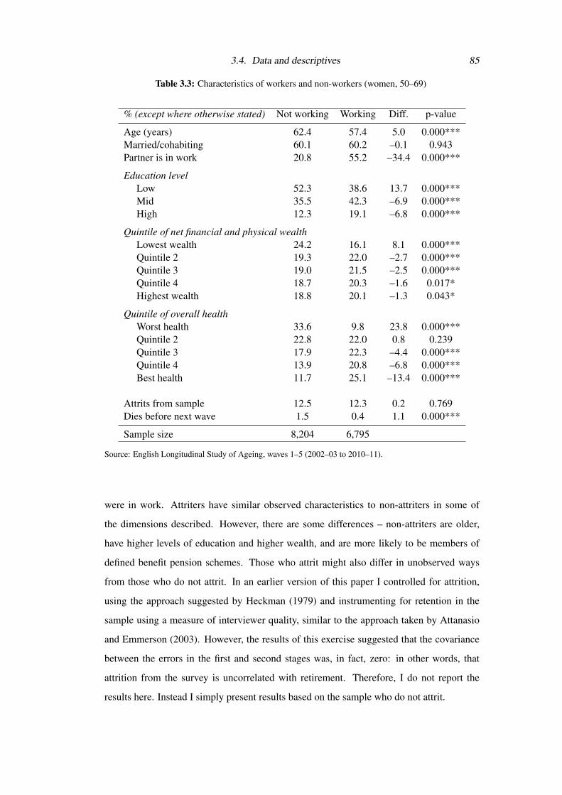
3.4. Data and descriptives 85
Table 3.3: Characteristics of workers and non-workers (women, 50–69)
% (except where otherwise stated) Not working Working Diff. p-value
Age (years) 62.4 57.4 5.0 0.000***Married/cohabiting 60.1 60.2 –0.1 0.943Partner is in work 20.8 55.2 –34.4 0.000***
Education levelLow 52.3 38.6 13.7 0.000***Mid 35.5 42.3 –6.9 0.000***High 12.3 19.1 –6.8 0.000***
Quintile of net financial and physical wealthLowest wealth 24.2 16.1 8.1 0.000***Quintile 2 19.3 22.0 –2.7 0.000***Quintile 3 19.0 21.5 –2.5 0.000***Quintile 4 18.7 20.3 –1.6 0.017*Highest wealth 18.8 20.1 –1.3 0.043*
Quintile of overall healthWorst health 33.6 9.8 23.8 0.000***Quintile 2 22.8 22.0 0.8 0.239Quintile 3 17.9 22.3 –4.4 0.000***Quintile 4 13.9 20.8 –6.8 0.000***Best health 11.7 25.1 –13.4 0.000***
Attrits from sample 12.5 12.3 0.2 0.769Dies before next wave 1.5 0.4 1.1 0.000***
Sample size 8,204 6,795
Source: English Longitudinal Study of Ageing, waves 1–5 (2002–03 to 2010–11).
were in work. Attriters have similar observed characteristics to non-attriters in some of
the dimensions described. However, there are some differences – non-attriters are older,
have higher levels of education and higher wealth, and are more likely to be members of
defined benefit pension schemes. Those who attrit might also differ in unobserved ways
from those who do not attrit. In an earlier version of this paper I controlled for attrition,
using the approach suggested by Heckman (1979) and instrumenting for retention in the
sample using a measure of interviewer quality, similar to the approach taken by Attanasio
and Emmerson (2003). However, the results of this exercise suggested that the covariance
between the errors in the first and second stages was, in fact, zero: in other words, that
attrition from the survey is uncorrelated with retirement. Therefore, I do not report the
results here. Instead I simply present results based on the sample who do not attrit.
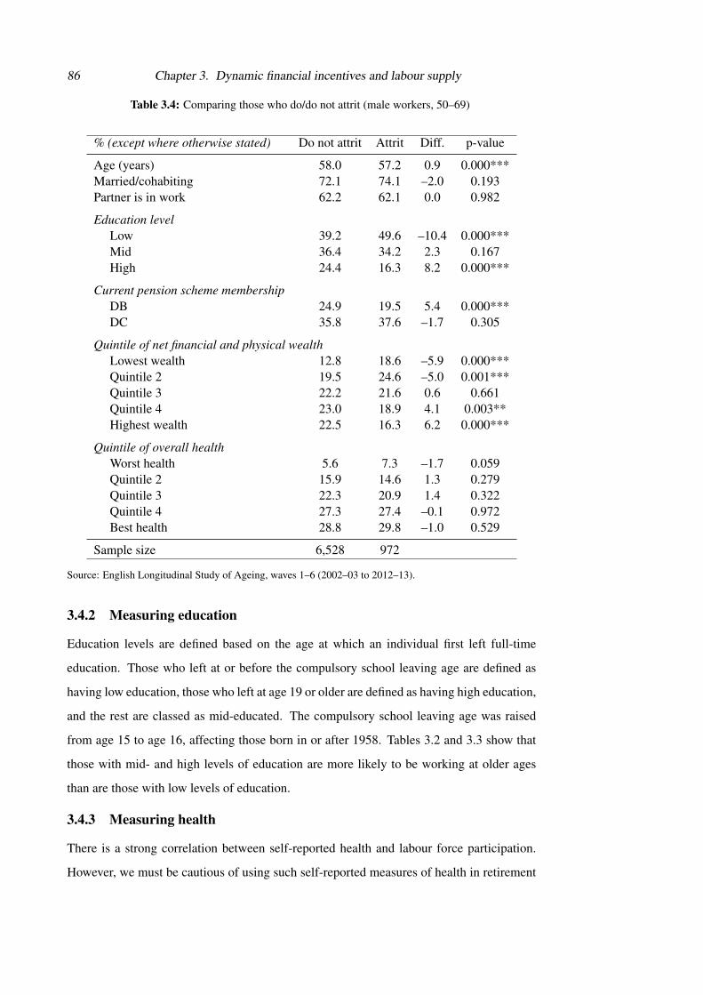
86 Chapter 3. Dynamic financial incentives and labour supply
Table 3.4: Comparing those who do/do not attrit (male workers, 50–69)
% (except where otherwise stated) Do not attrit Attrit Diff. p-value
Age (years) 58.0 57.2 0.9 0.000***Married/cohabiting 72.1 74.1 –2.0 0.193Partner is in work 62.2 62.1 0.0 0.982
Education levelLow 39.2 49.6 –10.4 0.000***Mid 36.4 34.2 2.3 0.167High 24.4 16.3 8.2 0.000***
Current pension scheme membershipDB 24.9 19.5 5.4 0.000***DC 35.8 37.6 –1.7 0.305
Quintile of net financial and physical wealthLowest wealth 12.8 18.6 –5.9 0.000***Quintile 2 19.5 24.6 –5.0 0.001***Quintile 3 22.2 21.6 0.6 0.661Quintile 4 23.0 18.9 4.1 0.003**Highest wealth 22.5 16.3 6.2 0.000***
Quintile of overall healthWorst health 5.6 7.3 –1.7 0.059Quintile 2 15.9 14.6 1.3 0.279Quintile 3 22.3 20.9 1.4 0.322Quintile 4 27.3 27.4 –0.1 0.972Best health 28.8 29.8 –1.0 0.529
Sample size 6,528 972
Source: English Longitudinal Study of Ageing, waves 1–6 (2002–03 to 2012–13).
3.4.2 Measuring education
Education levels are defined based on the age at which an individual first left full-time
education. Those who left at or before the compulsory school leaving age are defined as
having low education, those who left at age 19 or older are defined as having high education,
and the rest are classed as mid-educated. The compulsory school leaving age was raised
from age 15 to age 16, affecting those born in or after 1958. Tables 3.2 and 3.3 show that
those with mid- and high levels of education are more likely to be working at older ages
than are those with low levels of education.
3.4.3 Measuring health
There is a strong correlation between self-reported health and labour force participation.
However, we must be cautious of using such self-reported measures of health in retirement
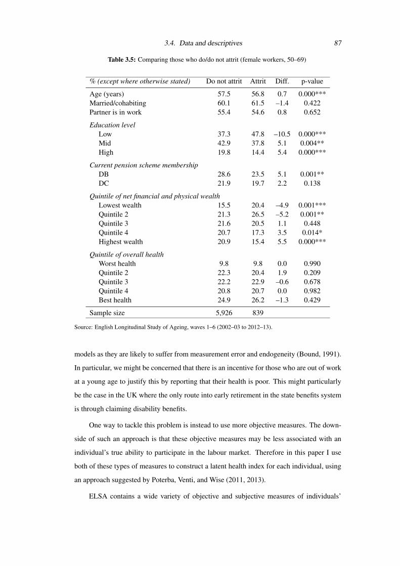
3.4. Data and descriptives 87
Table 3.5: Comparing those who do/do not attrit (female workers, 50–69)
% (except where otherwise stated) Do not attrit Attrit Diff. p-value
Age (years) 57.5 56.8 0.7 0.000***Married/cohabiting 60.1 61.5 –1.4 0.422Partner is in work 55.4 54.6 0.8 0.652
Education levelLow 37.3 47.8 –10.5 0.000***Mid 42.9 37.8 5.1 0.004**High 19.8 14.4 5.4 0.000***
Current pension scheme membershipDB 28.6 23.5 5.1 0.001**DC 21.9 19.7 2.2 0.138
Quintile of net financial and physical wealthLowest wealth 15.5 20.4 –4.9 0.001***Quintile 2 21.3 26.5 –5.2 0.001**Quintile 3 21.6 20.5 1.1 0.448Quintile 4 20.7 17.3 3.5 0.014*Highest wealth 20.9 15.4 5.5 0.000***
Quintile of overall healthWorst health 9.8 9.8 0.0 0.990Quintile 2 22.3 20.4 1.9 0.209Quintile 3 22.2 22.9 –0.6 0.678Quintile 4 20.8 20.7 0.0 0.982Best health 24.9 26.2 –1.3 0.429
Sample size 5,926 839
Source: English Longitudinal Study of Ageing, waves 1–6 (2002–03 to 2012–13).
models as they are likely to suffer from measurement error and endogeneity (Bound, 1991).
In particular, we might be concerned that there is an incentive for those who are out of work
at a young age to justify this by reporting that their health is poor. This might particularly
be the case in the UK where the only route into early retirement in the state benefits system
is through claiming disability benefits.
One way to tackle this problem is instead to use more objective measures. The down-
side of such an approach is that these objective measures may be less associated with an
individual’s true ability to participate in the labour market. Therefore in this paper I use
both of these types of measures to construct a latent health index for each individual, using
an approach suggested by Poterba, Venti, and Wise (2011, 2013).
ELSA contains a wide variety of objective and subjective measures of individuals’

88 Chapter 3. Dynamic financial incentives and labour supply
Figure 3.4: Average health percentile, by age and sex
Notes: Individuals are ranked according to their health, as measured by the health index, from the least healthy
to the healthiest. Figures are unweighted.
Source: English Longitudinal Study of Ageing, waves 1–6 (2002–03 to 2012–13).
physical and mental health and cognition. I use 23 separate measures of health to estimate
a principal components model and use the first principal component to rank individuals
according to their health level. The 23 health indicators that I use are shown in Table 3.6,
along with the estimated factor loadings. The health measures included in the index are not
a comprehensive list of all the measures available from ELSA but are those that are most
likely to be related to labour force participation. Tables 3.2 and 3.3 show that there is a
strong relationship between this summary measure of health and employment among those
aged 50–69: among both men and women, workers have much better health on average than
non-workers according to this index.
The index estimated varies across individuals and over time. To illustrate how this
index varies with age and across men and women, Figure 3.4 shows the average rank of
individuals of a given age and sex, according to this index – where a higher rank indicates
better health. This figure shows that, at a given age, men’s health is better on average than
women’s and that on average health deteriorates with age.

3.4. Data and descriptives 89
Table 3.6: First principal component of health: men and women
Factor loading
Has difficulty...walking quarter of a mile 0.289lifting or carrying 0.289pushing or pulling 0.284climbing several flights of stairs 0.283stooping/kneeling/crouching 0.278getting up from a chair 0.274reaching/extending arms 0.209sitting for two hours 0.222picking up a 5p piece 0.159with any ADL 0.281
Self-rated health: fair, poor 0.248
Ever been diagnosed with...Arthritis 0.205Psychological conditions 0.059Stroke 0.092Hypertension 0.142Lung disease 0.095Cancer 0.039Heart problems 0.123Diabetes 0.086
BMI 0.111BMI squared 0.112
Experiences any pain 0.249Experiences moderate or severe pain 0.260
Sample size 63,227
Notes: Table reports the factor loading of each indicator for the first principal component of health. Source:
English Longitudinal Study of Ageing, waves 1–6 (2002–03 to 2012–13).

90 Chapter 3. Dynamic financial incentives and labour supply
The health index is estimated separately for each individual in each wave using a
pooled sample of observations from all the waves. The ranking of individuals into quin-
tiles is then done using the pooled sample of individual observations of people aged 50–69
who are in work to ensure that one-fifth of my regression sample is assigned to each quintile.
3.4.4 Survival probabilities
The value that an individual will place on additional accrual of pension entitlements depends
importantly on how long she expects to live for. As shown in Equation 3.1, I assume that
individuals weight income in future years by the probability that they will still be alive at
that point. I base these probabilities on sex-specific period life tables produced by the Office
for National Statistics (Office for National Statistics, 2012).22 However, I adjust these life
tables to take account of differences in life expectancy between socioeconomic groups.
The ONS do not produce full life tables separately for different socioeconomic groups.
However, they do periodically publish figures comparing the average life expectancy of dif-
ferent groups. These suggest, in keeping with other evidence (see, for example, Attanasio
and Emmerson, 2003), that those in the highest socioeconomic groups live longer, on aver-
age, than those in lower socioeconomic groups.23 For example, figures from the ONS sug-
gest that, at the age of 65, men in the highest social class have a life expectancy that is 23%
longer than those in the lowest social class (Office for National Statistics, 2011). Failing to
account for this variation across socioeconomic groups would lead me to under-estimate the
value of accrued pension rights and future accrual for those in the highest socioeconomic
groups, and to over-estimate it for those in the lowest socioeconomic groups.
I adjust the official life table survival probabilities to account for these differences. To
do this I assume that the life table survival probabilities for each group follow a Weibull
distribution, with a common shape parameter but group-specific scale parameter. I use
the average social class-specific life expectancies published by the ONS to calculate the
resultant group-specific survival probabilities from the population-average life tables.
22Specifically, I use mortality probabilities based on data from 2007 to 2009. Unfortunately, official UK lifetables on a cohort basis are not available for the cohorts I examine here. The period life tables that I use maysomewhat understate the true value of individuals’ future pension income, although the additional years of life(which occur many years post-retirement) will be heavily discounted in the option value.
23It is worth noting, however, that this correlation is not necessarily causal. The evidence presented inChapter 4, suggests that there is little residual relationship between mortality and indicators of socioeconomicstatus once one has controlled for differences in diagnosed health conditions and health behaviours.
3.4. Data and descriptives 91
3.4.5 Calculating private pension entitlements
To identify the effect of pension incentives on individual retirement behaviour, I require
variation in the pension incentives that individuals face. As mentioned in Section 3.2, there
is considerable variation in the pension incentives that workers in England face. Much of
this is likely to be exogenous to individuals’ preferences for work. However, in order to
exploit this variation, I need accurate measures of pension entitlements and incentives for
respondents to the ELSA survey. This subsection explains how I have calculated private
pension entitlements and the next subsection describes the calculation of state pension enti-
tlements.
There are two main types of private pension – DB and DC – and I take a different
approach to calculating respondents’ entitlement to each of these types of scheme. DB
pensions are ones from which the benefit received depends on some function of (typically,
final)24 salary and years of membership. ELSA respondents are asked to report all the main
details of their DB pension scheme, including the measure of salary that benefits depend
on, the accrual fraction, years of membership, the normal pension age, and how benefits are
uprated post-retirement. These pieces of information are crucial if one wants accurately to
calculate the accrual incentives inherent in DB pension schemes. ELSA is the first survey
in the UK to provide this level of detail.
Using this information, it is relatively easy to calculate the level of annual pension
income that the individual could expect to get if she retired immediately.25 In order to
simulate what pension she would get if she were to continue working, I have to make some
assumption about future earnings growth. Based on earnings growth observed among ELSA
respondents who remain in work, I assume that earnings growth is 2.5% above inflation in
each year until the age of 55, after which I assume individuals experience no real earnings
growth.26
DC pensions involve contributions being made to a fund, which is invested and then
used to purchase an annuity at retirement.27 The pension income ultimately received from
24Recent reforms to public sector DB pension schemes have changed the rules so that pension benefits willin future depend on career-average, rather than final, salary. However, these changes were only implementedafter the period I am studying.
25I assume that drawing a pension before the normal pension age incurs an actuarial reduction of 4% peryear. This is the most common reduction used by schemes (Government Actuary’s Department, 2003).
26These assumptions are based on the changes observed between the first and second waves of ELSA,described in Banks, Emmerson, and Tetlow (2007a).
27Until April 2015 it was a legal requirement in the UK that at least three-quarters of the funds held in aDC pension be used to purchase an annuity by the time the pension holder reached age 75. The remaining

92 Chapter 3. Dynamic financial incentives and labour supply
a DC pension therefore depends on the level of contributions made, the investment returns
received, and the annuity rates available at the point of annuitisation. ELSA respondents
are asked to report the current value of their pension fund. To calculate the pension income
that an individual would receive if she retired immediately, I multiply this fund value by an
age- and sex-specific annuity rate.28
Calculating the pension income that would be received if an individual continued to
work requires some assumptions about how contributions will evolve in future and what
the investment return on the fund will be. I assume that pension funds will receive a real
investment return of 2.5% and that individuals will continue contributing to their pension
fund in the way that they did in the year prior to interview. Specifically, I assume that in-
dividuals who reported a cash amount for their pension contributions continue contributing
the same cash amount, while those who reported contributing an amount as a percentage of
salary continue contributing the same percentage of salary.29 I make the same assumptions
as outlined above about the future evolution of earnings.
If a sample member was unable to report any of the key pension scheme details, I
imputed the missing values using a conditional hotdeck. Further details on how private
pension entitlements are calculated is provided in Banks, Emmerson, and Tetlow (2005)
and Crawford (2012).
3.4.6 Calculating state pension entitlements
State pension entitlements depend on individuals’ employment, earnings and various other
activities (such as looking after children) over their lifetimes.30 Therefore, in order to es-
timate individuals’ state pension entitlements, I had to construct lifetime employment and
earnings profiles for all sample members. I did this in two steps: first estimating what an
individual’s earnings would have been in each previous year if she had been in work, then
determining whether or not she was in work in each year.
one-quarter could be taken as a tax-free lump sum. In March 2014 the government (unexpectedly) announcedthat these rules would be changed, with effect from April 2015. However, the data used in this paper relate to aperiod before this policy change was announced.
28The annuity rate used is the second-best rate for a level (i.e. not inflation-indexed) annuity that wasavailable in January 2005.
29These assumptions are based on the behaviour observed over time among the ELSA sample – see Banks,Emmerson, and Tetlow (2007a) for a description of changes in DC pension contributions between the first andsecond waves of ELSA.
30This method of computing future state pension entitlements assumes that individuals understand the rulesof the system and hold static expectations about future policy. Chan and Stevens (2004) and Bottazzi, Jappelli,and Padula (2006) demonstrate that individuals respond more strongly to what they believe the rules of thesystem are, rather than the actual rules. However, I do not attempt here to take account of any misperceptionsabout the rules of the state pension system.

3.4. Data and descriptives 93
Following a similar method to that employed by Blundell, Meghir, and Smith (2002,
2004), I assume that the potential earnings of individual i in cohort/education group g in
period t can be expressed as shown in Equation 3.10.
Wigt = θiWgt (3.10)
where θi is a constant individual fixed effect and Wgt is median earnings of cohort/education
group g estimated using data from the Living Costs and Food Survey (formerly the Ex-
penditure and Food Survey and, before that, the Family Expenditure Survey). θi is cal-
culated as the ratio between each individual’s earnings in ELSA and their group’s median
earnings in the same year.
Individuals are divided into three education groups, as described above. In order to
boost sample sizes, I pool together three consecutive year-of-birth cohorts and three consec-
utive years of observed earnings, with earnings from different years being inflated/deflated
using average earnings growth to make them comparable.
I assume that everyone was in work (and earning the wages just described) in each year
since leaving full-time education. This is a rather crude assumption, especially for women
in these cohorts. It could be improved upon by making use of linked administrative data that
is now available from individuals’ NI records. This should be a priority for future work.
If anything, the crude assumptions I make here are likely to lead to me over-estimating
accrued state pension entitlements, particularly for women; therefore, I may under-estimate
the true option value of remaining in work for an additional year.31 However, the assump-
tions I make about past earnings have less impact on the estimation of accrued state pension
entitlements than might be expected because the state pension system in the UK contains
significant ‘crediting’, which means that many individuals have accrued entitlement in past
years even if they were not in paid work.
It is worth emphasising, however, that the estimates of private pension entitlements and
accruals do not rely on these earnings and employment histories, since individuals report
directly their membership of and entitlements to private pension schemes (as described
above).
Table 3.7 describes the distribution of private and state pension wealth and measures
31See Bozio et al. (2010) for a description of how state pension entitlements calculated using the methoddescribed here compare to those calculated from the administrative records for the subset of ELSA respondentsfor whom linked administrative data are available.

94 Chapter 3. Dynamic financial incentives and labour supply
Table 3.7: Distribution of earnings, pension wealth and accrual measures
p25 Median p75 Mean St. dev.
MenEarnings (£000s) 17.6 26.7 40.3 34.3 45.8Private pension wealth (£000s) 31.1 125.2 294.9 220.9 415.5State pension wealth (£000s) 79.0 106.6 145.9 115.8 49.0One-period accrual (£000s) 1.4 3.7 7.8 5.6 13.2One-period accrual (as % of earnings) 4.5 16.0 30.3 15.5 448.8Peak value accrual (£000s) 2.5 9.1 21.8 20.2 43.3Peak value accrual (as % of earnings) 10.7 36.8 81.0 86.5 647.5Option value 2.5 7.9 14.7 10.4 12.3
WomenEarnings (£000s) 7.3 14.1 23.5 20.1 37.4Private pension wealth (£000s) 0.0 33.7 130.1 103.6 237.7State pension wealth (£000s) 70.3 105.6 137.7 105.2 56.2One-period accrual (£000s) 0.0 3.4 6.9 4.7 10.3One-period accrual (as % of earnings) 0.0 23.0 44.8 24.7 696.3Peak value accrual (£000s) 1.1 9.9 21.9 16.4 25.4Peak value accrual (as % of earnings) 10.3 73.6 140.5 148.9 1,377.1Option value 1.3 5.0 10.0 7.1 9.7
Notes: Monetary figures are expressed in 2015 prices.
Source: English Longitudinal Study of Ageing, waves 1–5 (2002–03 to 2010–11).
of pension accrual among my sample. As well as showing the distribution of the option
value, the table also shows the distribution of two other simpler financial incentive measures.
These are the one-period accrual (i.e. the present discounted value of the additional future
pension income accrued from one more year’s work) and the peak value accrual (i.e. the
maximum additional present discounted value of extra future pension income that could be
accrued by continuing to work). This shows that most men and women have some private
and state pension wealth. Among men, private pension entitlements are on average higher
than state pension entitlements. Among women the reverse is true. However, among both
men and women there is much greater dispersion of private pension rights than state pension
rights, which is to be expected given the institutional structures.
3.4.7 Constructing the option value
Calculating the option value of remaining in work requires examining the stream of income
that individuals receive from the age that they appear in the survey until they die. This
income stream will depend on the age at which they choose to retire. In calculating the
option values, I assume that individuals claim any private and state pensions to which they

3.4. Data and descriptives 95
are entitled at the point they ‘retire’.32 I also assume that families claim any means- and
asset-tested benefits to which they are entitled in each year.
In practice, individuals can choose to draw their state and private pensions at different
points in time – for example, deferring their state pension while starting to receive income
from a private pension. There are potentially financial incentives to do this (e.g. in order
to smooth marginal tax rates over time). Here I make the simplifying assumption that all
pensions are drawn at the same time, since incorporating different claiming dates is not
really consistent with the underlying spirit of the option value model. Modelling separate
claim dates would also be computationally difficult in a dynamic programming model, as
it would expand the choice set and state space. I am not aware of any papers that have
estimated a stochastic dynamic programming model of consumption and labour supply of
older people that incorporates separate choices about claiming state and private pensions.
As described in Section 3.3, the (utility) value to an individual of retiring at a particular
point in time is a function of the earned income that she will receive until she retires and the
retirement income she receives thereafter. I estimate the value of retiring at each age from
50 to 69, using the formula outlined in Equation 3.1. The option value is then calculated
as the difference between the value of retiring at the age that maximises this value function
and the value of retiring immediately (Equation 3.2).
In the ELSA data I observe current earnings for my baseline sample. In constructing
the option value measures, I assume that those who remain in paid work will receive the
same real terms income in every future year; the exception to this is that I assume individuals
receive 2.5% a year real earnings growth between the ages of 50 and 54.33 Private and state
pension entitlements, conditional on some future date of retirement, are calculated in the
way described in Sections 3.4.5 and 3.4.6, respectively.
The availability of (non-time-limited) means-tested benefits is factored into potential
income both before and after retirement in the option value calculations. Entitlement to
means-tested benefits depends on total family income (and assets). Therefore, in order to
calculate how much means-tested benefit income an individual might receive if she were not
working, I need to make some assumptions about her partner’s earnings and other income
32The only exception to this is private pensions to which individuals have retained rights but that they nolonger contribute to and from which they are not yet drawing an income. I assume that these are drawn at thestate pension age (regardless of the age of retirement).
33As mentioned above, this assumption is based on the changes in earnings that were observed between thefirst two waves of ELSA (see Banks, Emmerson, and Tetlow, 2007a).

96 Chapter 3. Dynamic financial incentives and labour supply
as well. To calculate family means-tested benefit income, if the individual’s partner is in
work at baseline, I assume that the partner remains in work until their state pension age. If
the partner is not working at baseline, I assume he remains out of work.
For each future year I calculate the means-tested benefit income that the family would
be entitled to by applying the rules of the benefit system to the income (from state and
private pensions) that the family would have in a particular year under each possible as-
sumption about the timing of retirement. There is also an asset test for receipt of means-
tested benefits in the UK – that is, assets above a certain threshold are assumed to generate
an income, which results in the withdrawal of some or all of the benefit. Therefore, I also
assess the family’s net financial wealth holdings against this asset test. To do this, I assume
that families’ wealth remains constant in real terms in future. The two main means-tested
benefits that I model are JSA (for working age individuals) and pension credit (for those
aged over the female state pension age), as described in Section 3.2.
Finally, I calculate sample members’ net income from all of the above sources by
calculating their liability to income tax and employee’s social insurance contributions. The
latter only applies to earnings received while aged below the state pension age. This allows
me to take into account the fact that additional accrual of pension rights would be valued
less by someone who faced a high marginal tax rate in retirement than by someone who
faced a low marginal rate.
Table 3.7 shows that there is considerable variation in the option values that individuals
face.
3.4.8 Prevalence of retirement
In this paper, the outcome that I examine is whether or not older people remain in or leave
paid work. Figure 3.5 shows what fraction of those aged between 50 and 69, who were in
work in one wave of ELSA, had ‘retired’ over the following two years, where ‘retirement’ is
defined as no longer doing any paid work. This is based on a question which asks individuals
whether they had done any work for pay in the last month prior to the survey – this includes
both working as an employee and being self-employed. The figure shows, as expected, that
older individuals are much more likely than younger individuals to leave work. Exit rates
are only slightly higher for women than men in almost all these age groups. The major
exception is at ages 55–59 when women are much more likely than men to leave work; this
reflects the fact that the state pension age for women was age 60 for most of the period
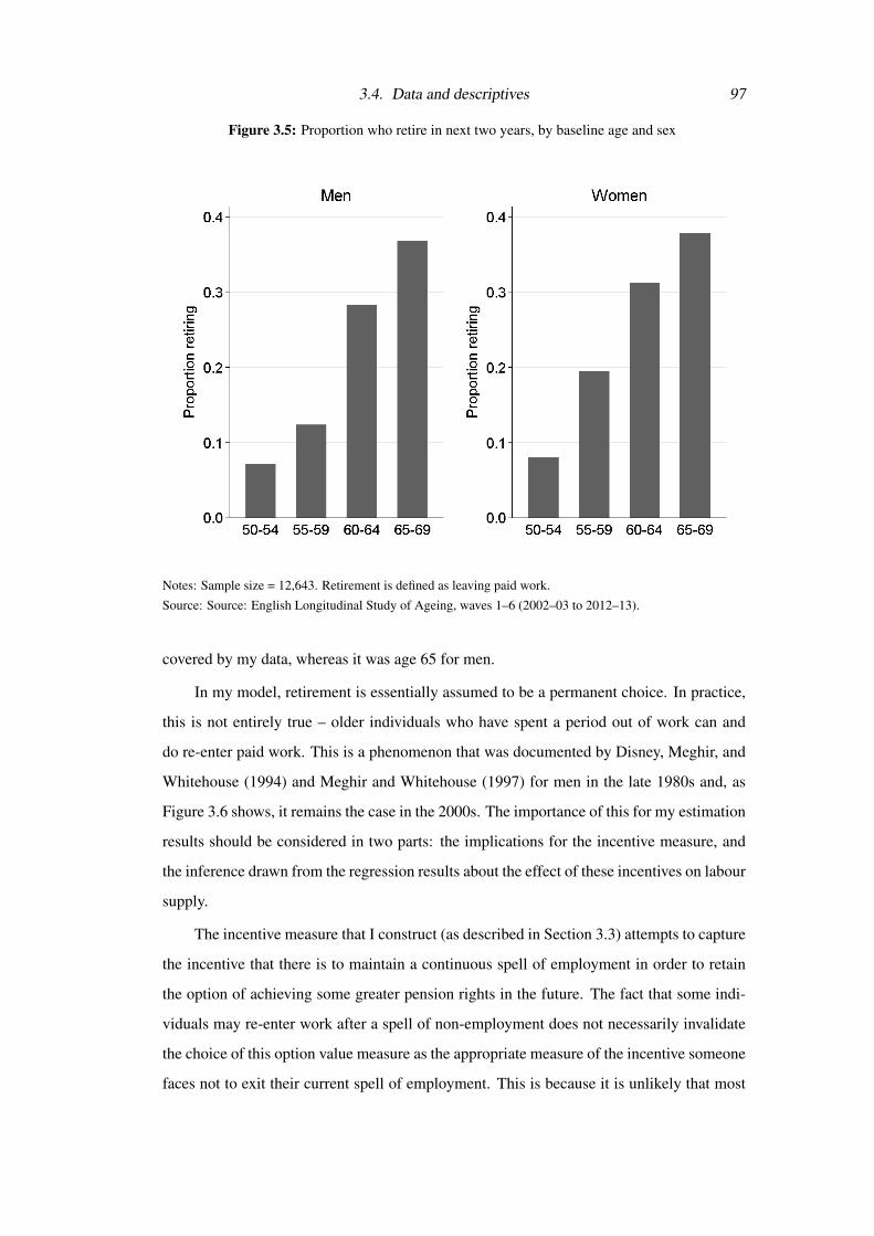
3.4. Data and descriptives 97
Figure 3.5: Proportion who retire in next two years, by baseline age and sex
Notes: Sample size = 12,643. Retirement is defined as leaving paid work.
Source: Source: English Longitudinal Study of Ageing, waves 1–6 (2002–03 to 2012–13).
covered by my data, whereas it was age 65 for men.
In my model, retirement is essentially assumed to be a permanent choice. In practice,
this is not entirely true – older individuals who have spent a period out of work can and
do re-enter paid work. This is a phenomenon that was documented by Disney, Meghir, and
Whitehouse (1994) and Meghir and Whitehouse (1997) for men in the late 1980s and, as
Figure 3.6 shows, it remains the case in the 2000s. The importance of this for my estimation
results should be considered in two parts: the implications for the incentive measure, and
the inference drawn from the regression results about the effect of these incentives on labour
supply.
The incentive measure that I construct (as described in Section 3.3) attempts to capture
the incentive that there is to maintain a continuous spell of employment in order to retain
the option of achieving some greater pension rights in the future. The fact that some indi-
viduals may re-enter work after a spell of non-employment does not necessarily invalidate
the choice of this option value measure as the appropriate measure of the incentive someone
faces not to exit their current spell of employment. This is because it is unlikely that most

98 Chapter 3. Dynamic financial incentives and labour supply
Figure 3.6: Proportion of non-workers who were in work two years later
Notes: Sample size = 17,590. Figure shows the proportion of non-workers who enter work over a two-year
period, split by whether or not they belong to a private pension scheme when they are in work.
Source: Source: English Longitudinal Study of Ageing, waves 1–6 (2002–03 to 2012–13).
individuals would be able to rejoin their pension scheme on the same terms as they are cur-
rently on, if they were to leave. Indeed, as Figure 3.6 shows, only a minority of those who
re-enter work at older ages gain private pension coverage of any sort. This same argument
does not apply to the state pension scheme. However, the financial incentives that individu-
als face to continue accruing state pension rights at the end of working life are rather small
in many cases because, as mentioned above, many individuals accrue little or no additional
state pension rights once they have achieved their full 30 years of contributions to the BSP.
Overall, therefore, the option value measure remains a reasonable measure of the incent-
ive someone faces not to exit their current employment spell even if some individuals do
re-enter the labour market after a spell of non-employment.
However, my regression results may nonetheless overstate the effect of financial in-
centives from pensions on labour supply of older people if some of those who are incentiv-
ised to leave work subsequently return. Meghir and Whitehouse (1997) adopted an alternat-
ive approach to allow for returns to, as well we exits from, work among men born between

3.5. Results 99
1919 and 1933 who were not members of an occupational pension scheme. They found that
the availability of out of work benefits, health and age were all important determinants of
the likelihood of re-entering work. However, they were not able to incorporate incentives
from pension schemes. Re-estimating a similar type of analysis using the more detailed,
more recent data available from ELSA would be an interesting exercise for future work but
is beyond the scope of this paper. To the extent that some of those who are incentivised (by
the option value) to end their current spell of employment subsequently return to work, my
regressions results may overstate the (negative) effect of financial incentives on the labour
supply of older workers. This should be borne in mind when interpreting the results.
3.5 Results
This section presents results from the model described in Section 3.3.2. I start by presenting
results from a random effects probit model for the relationship between financial incentives
and the probability of moving out of paid work for the sample as a whole (Section 3.5.1).
Section 3.5.2 examines whether the responsiveness of behaviour to financial incentives has
changed over time, while Section 3.5.3 examines whether the effects of financial incentives
differ for those in better and worse health.
3.5.1 Exits from paid work
Tables 3.8 and 3.9 present the results from four separate random effects probit models,
estimated using the sample of respondents aged under 70 in the first five waves of ELSA.
The standard errors are constructed in a way that allows for dependence over time in the
unobservables for the same individual.
The four models differ from one another in the way that they control for age and
earnings. Each of the models includes interaction terms between sex and the non-financial
variables – to allow for these variables to affect the labour supply behaviour of men and
women differently. The financial variables are not interacted with sex, thus restricting the
response to financial incentives to be the same for men and women. In an earlier version
of this paper, I also allowed for the effect of financial incentives to differ between men and
women but I found that there was not a statistically significant difference between the effects
for each.
Table 3.8 reports the average marginal effects for each of the regressors among men,
while Table 3.9 reports the average marginal effects among women. The marginal effect
100 Chapter 3. Dynamic financial incentives and labour supply
of each variable is calculated for each individual in the sample (first setting male = 1 and
then setting male = 0) and the figures reported in Tables 3.8 and 3.9 are the average of these
marginal effect values across the whole estimation sample.
Specification (1) includes a quadratic in age and no control for current earnings. Spe-
cification (2) includes dummy variables for each individual age group and no control for
earnings. Specification (3) includes a quadratic in age and a log earnings term, and Spe-
cification (4) includes age dummies and log earnings.
As discussed in Section 3.3, it is not entirely clear what the correct way to control for
age and earnings is. On the one hand, to the extent that individuals retire at a specific age
because of financial incentives to do so provided by their pension plan and/or remain in
work because of the financial incentive provided by high earnings, then these effects should
properly be captured by the option value term. In this case, controlling for age and earnings
separately will cause me to under-estimate the effect of the option value. On the other hand,
if (for example) the spikes in retirement at particular ages reflect social norms or higher
earners earn more because they have a higher preference for work than lower earners, then
excluding these variables from the regression would cause me incorrectly to assign these
effects to the option value. This is because both age and earnings feature in the option
value. I compare and discuss the four sets of results below.
The marginal effects of the non-financial variables in Tables 3.8 and 3.9 largely have
the signs that we would expect. Among both men and women, those in the worst health
quintile are significantly more likely to retire over the following two years than healthier
people. They are around 11 percentage points more likely to retire than the mid-health
group among both men and women and the size of this effect is largely invariant to the way
in which age and earnings are controlled for. This 11 percentage point effect compares to
an average exit probability of 17.6% among men and 20.3% among women in the sample.
Single men and men whose partner does not work have similar exit probabilities to one
another. In contrast, men whose wife was working are 7 percentage points less likely to exit
work over the following two years than the other groups. A different pattern is seen among
women. Single women and women with a working partner have similar exit probabilities,
while women with non-working partners are around 4 percentage points more likely to
retire than the others. However, it is not possible to tell from these results alone whether
the correlation is the result of a direct effect of partners’ work on individuals’ retirement
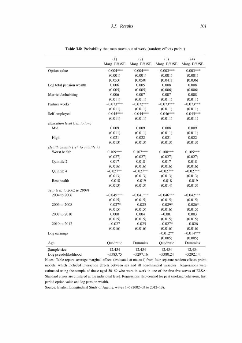
3.5. Results 101
Table 3.8: Probability that men move out of work (random effects probit)
(1) (2) (3) (4)Marg. Eff./SE Marg. Eff./SE Marg. Eff./SE Marg. Eff./SE
Option value –0.004*** –0.004*** –0.003*** –0.003***(0.001) (0.001) (0.001) (0.001)[0.053] [0.050] [0.041] [0.036]
Log total pension wealth 0.006 0.005 0.008 0.008(0.005) (0.005) (0.006) (0.006)
Married/cohabiting 0.006 0.007 0.007 0.008(0.011) (0.011) (0.011) (0.011)
Partner works –0.073*** –0.072*** –0.073*** –0.073***(0.011) (0.011) (0.011) (0.011)
Self-employed –0.045*** –0.044*** –0.046*** –0.045***(0.011) (0.011) (0.011) (0.011)
Education level (rel. to low)Mid 0.009 0.009 0.008 0.009
(0.011) (0.011) (0.011) (0.011)High 0.021 0.022 0.021 0.022
(0.013) (0.013) (0.013) (0.013)Health quintile (rel. to quintile 3)
Worst health 0.109*** 0.107*** 0.108*** 0.105***(0.027) (0.027) (0.027) (0.027)
Quintile 2 0.017 0.018 0.017 0.018(0.016) (0.016) (0.016) (0.016)
Quintile 4 –0.027** –0.027** –0.027** –0.027**(0.013) (0.013) (0.013) (0.013)
Best health –0.018 –0.019 –0.018 –0.019(0.013) (0.013) (0.014) (0.013)
Year (rel. to 2002 to 2004)2004 to 2006 –0.045*** –0.041*** –0.046*** –0.042***
(0.015) (0.015) (0.015) (0.015)2006 to 2008 –0.027* –0.025 –0.029* –0.026*
(0.015) (0.015) (0.016) (0.015)2008 to 2010 0.000 0.004 –0.001 0.003
(0.015) (0.015) (0.015) (0.015)2010 to 2012 –0.027 –0.025 –0.027* –0.026
(0.016) (0.016) (0.016) (0.016)Log earnings –0.012** –0.014***
(0.005) (0.005)Age Quadratic Dummies Quadratic Dummies
Sample size 12,454 12,454 12,454 12,454Log pseudolikelihood –5383.75 –5297.16 –5380.24 –5292.14
Notes: Table reports average marginal effects (evaluated at male=1) from four separate random effects probit
models, which included interaction effects between sex and all non-financial variables. Regressions were
estimated using the sample of those aged 50–69 who were in work in one of the first five waves of ELSA.
Standard errors are clustered at the individual level. Regressions also control for past smoking behaviour, first
period option value and log pension wealth.
Source: English Longitudinal Study of Ageing, waves 1–6 (2002–03 to 2012–13).

102 Chapter 3. Dynamic financial incentives and labour supply
behaviour or whether it simply reflects other differences between those with working and
non-working partners.
Among both men and women, those who are self-employed are found to be less likely
to exit paid work than those who are employees, all else equal. However, this effect is only
statistically significantly different from zero for men.
Among women (but not men) those with higher levels of education are more likely to
retire than those with lower levels of education. However, it is worth noting that (as Table
3.3 showed) low educated women are less likely than those with mid and high levels of
education to be in work in the first place.
Finally, there is no clear pattern to the time dummies. In general, it appears that retire-
ment rates were lower from 2004 onwards than between 2002 and 2004. This is broadly in
keeping with the observed growth in employment rates above age 50 over the last decade.
However, the marginal effects for the latest two periods (that is, 2008–09 to 2012–13) are
not statistically significantly different from the first period. Of course it is possible that this
reflects the net effect of off-setting factors – perhaps a general trend towards lower rates of
retirement being offset by the macroeconomic effects of the recession and weak economic
growth on job availability after 2008.
The main marginal effects of interest are those on the financial incentive measures.
The wealth effect is found to have the expected (positive) sign but not to be statistically
significantly different from zero in any of the specifications. The marginal effect of the
accrual incentive (captured by the option value) also has the expected sign – that is, a larger
option value of remaining in work is associated with a lower probability of retiring – and
this is strongly statistically significant in all the specifications.
For ease of interpretation, the figures reported in square brackets (below the marginal
effects and standard errors for the option value) show the average effect on the retirement
probability of a one standard deviation change in the option value – that is, moving everyone
from one standard deviation above their actual option value to one standard deviation below
it. Such a change would increase the retirement probability of men and women by between
3 and 5 percentage points (depending on the specification). This is an economically, as
well as statistically, significant effect. For example, it is equal to about a third to a half
of the difference in retirement rates seen between those in the worst health and those with
middling levels of health.

3.5. Results 103
Table 3.9: Probability that women move out of work (random effects probit)
(1) (2) (3) (4)Marg. Eff./SE Marg. Eff./SE Marg. Eff./SE Marg. Eff./SE
Option value –0.005*** –0.005*** –0.004*** –0.003***(0.001) (0.001) (0.001) (0.001)[0.047] [0.045] [0.036] [0.032]
Log total pension wealth 0.006 0.005 0.009 0.008(0.006) (0.006) (0.006) (0.006)
Married/cohabiting 0.040*** 0.041*** 0.037*** 0.038***(0.012) (0.012) (0.012) (0.012)
Partner works –0.043*** –0.042*** –0.043*** –0.041***(0.012) (0.012) (0.012) (0.012)
Self-employed –0.022 –0.021 –0.024 –0.023(0.016) (0.016) (0.015) (0.015)
Education level (rel. to low)Mid 0.022* 0.023* 0.023** 0.024**
(0.012) (0.012) (0.012) (0.012)High 0.045*** 0.047*** 0.048*** 0.050***
(0.016) (0.017) (0.016) (0.017)Health quintile (rel. to quintile 3)
Worst health 0.111*** 0.117*** 0.109*** 0.114***(0.022) (0.022) (0.022) (0.022)
Quintile 2 0.011 0.015 0.011 0.014(0.015) (0.015) (0.015) (0.015)
Quintile 4 –0.025* –0.022 –0.025 –0.021(0.015) (0.015) (0.015) (0.015)
Best health –0.030** –0.028* –0.029* –0.028*(0.015) (0.015) (0.015) (0.015)
Year (rel. to 2002 to 2004)2004 to 2006 –0.054*** –0.043*** –0.054*** –0.044***
(0.016) (0.016) (0.016) (0.016)2006 to 2008 –0.004 –0.008 –0.005 –0.009
(0.017) (0.017) (0.017) (0.017)2008 to 2010 –0.004 0.005 –0.006 0.002
(0.017) (0.017) (0.016) (0.016)2010 to 2012 –0.034* –0.029 –0.034* –0.029
(0.018) (0.018) (0.018) (0.018)Log earnings –0.013** –0.015***
(0.005) (0.005)Age Quadratic Dummies Quadratic Dummies
Sample size 12,454 12,454 12,454 12,454Log pseudolikelihood –5383.75 –5297.16 –5380.24 –5292.14
Notes: Table reports average marginal effects (evaluated at male=0) from four separate random effects probit
models, which included interaction effects between sex and all non-financial variables. Other notes as Table
3.8.
Source: As Table 3.8.

104 Chapter 3. Dynamic financial incentives and labour supply
Figure 3.7: Actual and predicted retirement hazards
Notes: Hazards shown are based on specifications (3) and (4) shown in Table 3.8 and 3.9.
Source: English Longitudinal Study of Ageing, waves 1–6 (2002–03 to 2012–13).
Comparing specifications (1) and (2), and (3) and (4), it is clear that adding age dum-
mies improves the fit of the model significantly compared to a quadratic specification – as
indicated by the log likelihoods. However, the alternative ways of controlling for age have
little effect on the marginal effect of the option value. This suggests that we may not be too
concerned about the option value inappropriately picking up an ‘age’ effect. It also suggests
that there may be two different types of people – those for whom focal ages are important
in determining the timing of retirement and those for whom financial incentives matter.
The failure of financial incentives to explain the pronounced spikes in retirement at
specific ages is further highlighted in Figure 3.7, which shows the predicted retirement
hazards from models (3) and (4) for men and women, compared to the observed retirement
hazards. This shows that the model with an age quadratic does not pick up the large spike
in retirements at around ages 60 (for women) and 65 (for both men and women). For this
reason, it seems better to use the model including full age dummies rather than the more
parsimonious specification of age.
Comparing specifications (2) and (4) shows the effect of controlling separately for log

3.5. Results 105
earnings. For women (though less so for men), including log earnings reduces the absolute
size of the marginal effect of the option value on retirement. As Coile and Gruber (2007)
point out, the option value can be dominated by the earnings that a person receives while
in work. However, high earners may also differ from low earners in other ways – such as
in their preference for work. It seems more cautious, therefore, to focus on the marginal
effects from specification (4), which controls separately for earnings, to minimise such
concerns about other unobserved heterogeneity being attributed to the option value. In an
earlier version of this paper I also estimated the alternative peak value model proposed
by Coile and Gruber (2007). The peak value measure of financial incentives, which does
not incorporate the value of future earnings, was also found to be a statistically significant
predictor of retirement for both men and women. For brevity I do not report the results here.
Even controlling separately for age dummies and for earnings, however, the option
value is found to have a statistically and economically significant effect on retirement prob-
abilities. The retirement hazards implied by specification (4) are shown for both men and
women in Figure 3.7.
3.5.2 Importance of financial incentives over time
As Section 3.2 described, the relationship between drawing a pension and quitting work
has been gradually weakened over time. The most significant change during the period I
examine here was the reform in 2006 to allow individuals to claim a pension from their
employer’s scheme while continuing to work for the same employer. Table 3.10 reports
the average marginal effects of the option value in each of the two-year periods covered by
my dataset. These average marginal effects are from a model similar to specification (4) in
Tables 3.8 and 3.9 but also including full interactions between the time period dummies and
the option value term.
A likelihood ratio test of this fully interacted model against the restricted model above
suggests that I cannot reject that the restricted model presented above is the correct model –
the p-value of this test is 0.284. In other words, there is no significant evidence that the aver-
age response to financial incentives was different across the different time periods covered
by the ELSA survey waves. It is not clear therefore that policy reforms that have weakened
the theoretical relationship between drawing a pension and leaving work have actually res-
ulted in a systematically weaker relationship between the dynamic financial incentives and
retirement over time.

106 Chapter 3. Dynamic financial incentives and labour supply
Table 3.10: Probability of leaving work: effect of the option value over time
2002 to 2004 2004 to 2006 2006 to 2008 2008 to 2010 2010 to 2012Marg. Eff./SE Marg. Eff./SE Marg. Eff./SE Marg. Eff./SE Marg. Eff./SE
Option value –0.005*** –0.003* –0.004*** –0.002* –0.003(0.002) (0.001) (0.001) (0.001) (0.002)[0.040] [0.028] [0.040] [0.029] [0.041]
Sample size 12,454 12,454 12,454 12,454 12,454Notes: Table reports average marginal effects (evaluated at each value of the time dummies) from a random
effects probit model, which includes all the same regressors as Specification (4) in Tables 3.8 and 3.9 plus
full interactions between time, sex, and the option value. The regression was estimated using the sample of
those aged 50–69 who were in work in one of the first five waves of ELSA. Standard errors are clustered at the
individual level. Regression also controls for past smoking behaviour, first period option value and log pension
wealth.
Source: As Table 3.8.
Table 3.11: Probability of leaving work: effect of the option value for different health quintiles
Worst Quintile 2 Quintile 3 Quintile 4 BestMarg. Eff./SE Marg. Eff./SE Marg. Eff./SE Marg. Eff./SE Marg. Eff./SE
Option value –0.002 –0.002 –0.004*** –0.003** –0.004***(0.002) (0.002) (0.001) (0.001) (0.001)[0.021] [0.027] [0.037] [0.031] [0.045]
Sample size 12,454 12,454 12,454 12,454 12,454Notes: Table reports average marginal effects (evaluated at each value of the health quintile) from a random
effects probit model, which includes all the same regressors as Specification (4) in Tables 3.8 and 3.9 plus
full interactions between health, sex, and the option value. The regression was estimated using the sample of
those aged 50–69 who were in work in one of the first five waves of ELSA. Standard errors are clustered at the
individual level. Regression also controls for past smoking behaviour, first period option value and log pension
wealth.
Source: As Table 3.8.
3.5.3 Does the importance of incentives vary with health?
The results presented in Tables 3.8 and 3.9 suggest that financial incentives are important,
on average, for explaining exits from work. However, it is also clear that other factors –
notably health – also affect employment of older people. Therefore, one interesting question
is whether financial incentives are important for all groups or whether there are some groups
for whom other considerations dominate. For example, do those in poor health respond in
the same way to financial incentives as those in good health?
There are a number of possible reasons why those in worse health may respond dif-
ferently to the financial incentive measure that I use than those in better health. First, those
in the worst health are likely to have shorter life expectancies than the average, meaning
that the measure of option value that I have constructed here may overstate the true value to

3.6. Simulating an increase in the state pension age 107
them of delaying retirement. Second, those in worse health may place different weights on
income versus leisure than those in better health. Third, it could be that the relevant option
for this group is to take disability benefits, which have not been factored into the modelling
here.
To examine this question, I re-estimated specification (4) including interaction terms
between the option value measure and the health quintile indicators. The average marginal
effects of the option value for each of the health quintile groups from this model are shown
in Table 3.11.
Interestingly, the marginal effect of the option value is estimated to have a smaller (and
not statistically significant) effect for those in the two worst health quintiles. However, a
likelihood ratio test suggests that I cannot reject the hypothesis that the coefficients on the
option value for each health group are the same (the p-value for this test is 0.554). This
suggests that those in poor health respond in the same way as those in better health to
financial incentives from state and private pension schemes.
3.6 Simulating an increase in the state pension age
One of the major reforms that has been made to the state pension system in the UK in recent
decades is to increase the age at which people can claim their pension. The state pension
age for women is currently increasing from age 60 (in 2010) to age 66 (in 2020), while
the state pension age for men will increase from age 65 to age 66 between 2018 and 2020.
Evaluating the actual effect of the increase in the female state pension age from 60 to 61 is
the subject of Chapter 2. However, in that chapter – to the extent that I attempt to unpick the
mechanisms driving the responses – I focus only on the impact of static financial incentives.
It is interesting therefore to use the model estimated here to simulate what effect this reform
might have through the dynamic financial incentives that it induces.
To do this, I re-computed the option value facing each individual under the assumption
that the state pension age for both men and women was increased by one year. This means
that the state pension age for men in the sample is increased to age 66 and the state pen-
sion age for (most) women in the sample is raised to age 61.34 I then simulate retirement
probabilities based on these new option values using the coefficients from specification (4)
in Tables 3.8 and 3.9. Figure 3.8 shows the resulting 2-year retirement hazards. Figure 3.9
34Women born from 1950 onwards actually face a state pension age above 60 and so in my simulation willface a state pension age above 61.

108 Chapter 3. Dynamic financial incentives and labour supply
Figure 3.8: Predicted effect of increasing the state pension age by one year on retirement hazards
Notes: Hazards calculated from marginal effects using specification (4) shown in Tables 3.8 and 3.9. The figures
shows two alternative predictions for the effect of increasing the SPA by one year: (i) assuming that the age
effects remain the same, (ii) assuming that the age effects are also delayed by one year.
Source: English Longitudinal Study of Ageing, waves 1–6 (2002–03 to 2012–13).
uses these hazards to construct a survival curve – showing what fraction of those who were
in work at age 51 would still be in work at later ages.
In each figure I present two alternative simulations. The first assumes that only the
option value changes when the pension age increases (i.e. the age effects remain fixed).
The second assumes that the age effects also shift by one year – this is akin to believing
that the age effects capture ‘the effect of being X years from the state pension age’. It is
clear that changes to the option value alone have very little effect on simulated retirement
behaviour. The reform marginally increases the option value of remaining in work and so
the predicted retirement rates are slightly lower than those based on the original data, with
this effect being larger for men than for women. The impact of the reform is, unsurprisingly,
far more pronounced if I also move the age effects.
It is interesting to compare these predictions to the findings in Chapter 2. Figure 3.9
suggests that, under the reformed system, by the age of 60, 50% of those who were in
work at the age of 51 would still be working (if we do not shift the age dummies). The

3.7. Conclusions 109
figure would be 59% if we do shift the age dummies. This compares to 47% based on the
actual data. 84% of 51 year-old women were in work in 2012–13. This suggests that the
difference in the employment rate at age 60 between the reformed and unreformed systems
would be 3 percentage points, assuming the age effects do not shift, or 10 percentage points,
if the age effects do shift. This compares to a 7 percentage point effect found in Chapter
2. This suggests that the change in the dynamic financial incentives alone are not sufficient
to explain the size of the increase in female employment that was seen in response to the
recent increase in the female state pension age.
3.7 Conclusions
This paper presents evidence on the dynamic financial incentives facing older workers in
England and evaluates what effect these have on retirement behaviour. I do this using a
version of the option value model proposed by Stock and Wise (1990). I find that the dy-
namic financial incentives inherent in the state and private pension systems and the tax and
benefit system have had an economically and statistically significant effect on the retirement
behaviour of men and women aged between 50 and 69 over the last decade.
This suggests that changes to the dynamic financial incentives that individuals face
could further increase employment rates of older people. Some changes are already hap-
pening. In particular, DB pensions are increasingly rare in the private sector and are instead
being replaced by DC pensions, which have different incentive structures. Changes are also
being made to the state pension – increasing the state pension age but also reducing the mar-
ginal accrual for many people at the end of working life. The results presented here suggest
that these sorts of changes to financial incentives will have some effect on retirement be-
haviour – the increase in the state pension age is likely to raise retirement ages, while the
reduced accrual is likely to lower retirement ages as it reduces the incentive to remain in
work.
However, despite the significant relationship that I find between financial incentives
and retirement, I still find that these financial incentives alone are unable to explain the most
striking patterns in retirement behaviour in England. In particular, the dynamic financial
incentives do not predict the large spikes in retirement at the male and female state pension
ages. Since these age ‘effects’ appear to be uncorrelated with the financial incentives, it
appears that there are two distinct types of people – those who retire at focal ages and those
who respond to financial incentives.

110 Chapter 3. Dynamic financial incentives and labour supply
Figure 3.9: Predicted effect of increasing the state pension age by one year on fraction remaining inwork
Notes: Survival curves based on marginal effects using specification (4) shown in Tables 3.8 and 3.9. The
figures shows two alternative predictions for the effect of increasing the SPA by one year: (i) assuming that the
age effects remain the same, (ii) assuming that the age effects are also delayed by one year.
Source: English Longitudinal Study of Ageing, waves 1–6 (2002–03 to 2012–13).

3.7. Conclusions 111
While it is possible that a full dynamic programming model of retirement decision-
making could fit observed behaviour more closely than the option value approach here, it
seems unlikely that financial incentives alone can explain the patterns of retirement beha-
viour that are observed. There are no strong financial incentives for most individuals in the
UK to retire at ages 60 or 65 and yet this has remained the predominant pattern over the
last decade. This suggests that a priority for future work should be to understand better the
other non-financial factors that determine when many older individuals retire.

Chapter 4
Misperceived chances of survival:
Implications for economic behaviour
4.1 Introduction1
The life-cycle model of consumption and saving is well-established in the economic literat-
ure (Fischer, 1930; Modigliani and Brumberg, 1954). Such models have formed the back-
bone of work in economics seeking to understand how individuals make decisions about
consumption, saving and labour supply over their lifetimes. Yaari (1965) was the first to in-
corporate an uncertain length of life into a model of optimal lifetime consumption and this
feature of life-cycle models has since become commonplace. Such models make important
assumptions about the probability distribution over individuals’ future survival and what
individuals know about this. These assumptions are important because, as Arthur (1981)
showed, changing survival probabilities in such a model affects life-cycle maximisation.
Most life-cycle models in the literature (see, for example, Rust and Phelan, 1997) as-
sume that individuals face the average age- and sex-specific survival probabilities in their
country and that they have rational expectations about their chances of survival. Both of
these are potentially strong assumptions. On the one hand, there is a wealth of epidemi-
ological evidence that suggests that survival probabilities vary systematically with certain
characteristics (for example, socioeconomic status and health behaviours). Individuals have
a lot of information about their own circumstances and behaviour and may take the effect
of these on their survival chances into account when making decisions. On the other hand,
1I am grateful to Richard Blundell, Richard Disney and Carl Emmerson for helpful comments on earlierdrafts of this paper, to Cormac O’Dea for helpful comments and for his help in solving the example life-cyclemodels of behaviour and to Soumaya Keynes for providing me with access to her derived variables on theprevalence of health conditions in the English Longitudinal Study of Ageing.
114 Chapter 4. Misperceived chances of survival
particularly given the fairly rapid improvements that there have been over recent decades in
life expectancies, it is perhaps heroic to assume that all individuals are well informed about
the population average figures for people like them.
As Manski (2004) discusses, since observed choices may be consistent with many
alternative specifications of preferences and expectations, assuming erroneously that in-
dividuals hold rational expectations about population average survival probabilities may
lead to preference parameters (in particular, discount rates and risk aversion) being mis-
estimated. While quite a lot of attention has been devoted in the literature to estimating
variation in discount rates in the population (Samwick, 1998; Gustman and Steinmeier,
2005; Hendricks, 2007; Alan and Browning, 2010; Bozio, Laroque, and O’Dea, 2013), less
effort has been focussed on the potential importance for life-cycle behaviour of differences
in expected chances of survival.2 This is despite the fact that a number of household sur-
veys now attempt to elicit information on individuals’ own expectations of future survival.
Building heterogeneity in future survival probabilities into life-cycle models of consump-
tion and saving could be very important for helping to understand heterogeneous individual
responses, which could in turn affect how individuals respond to policy changes, and what
role there might be for further policy interventions.
In this paper, I use data from the English Longitudinal Study of Ageing (ELSA) to
show that on average people believe they face survival curves that are ‘flatter’ than life
tables suggest. I then use two simple life cycle models to demonstrate the implications
of this for consumption and saving and show that this phenomenon could help explain a
number of apparently puzzling aspects of individual behaviour: why people ‘undersave’
for retirement, why consumption drops sharply at retirement, why demand for annuities
is lower than standard models suggest it should be and why people decumulate wealth so
slowly at the end of life.
Section 4.2 starts by reviewing the existing literature on individuals’ expectations of
survival. Section 4.3 describes the ELSA survey data and Section 4.4 examines in detail
the responses provided to questions about survival to future older ages. Based on these
responses, Section 4.5 estimates the shape of individuals’ perceived survival curves and
discusses how much flatter these are than official life tables. Section 4.6 then presents
two simple life cycle models to show what implications these flatter survival curves could
2Gan, Hurd, and McFadden (2004) and van der Klaauw and Wolpin (2008) are exceptions.
4.2. Related literature 115
have for individuals’ behaviour compared to the standard assumption that individuals hold
rational expectations about their chances of survival based on life table values. Section 4.7
concludes.
4.2 Related literature
As Manski (2004) sets out, attitudinal researchers have for a long time tried to measure
individuals’ expectations using verbal questions – that is, asking individuals to express the
likelihood of some future event by picking from a range of categories, such as ‘very likely’,
‘fairly likely’, ‘not at all likely’. However, questions of this sort are difficult to use to
understand heterogeneity in individual behaviour and preferences for at least two reasons.
First, the response scales are very coarse and so the responses provide limited information.
Second, it is likely that respondents interpret these descriptive tags in different ways from
one another – meaning that the response scale may not be comparable across people (or,
indeed, for the same person at different points in time).
An alternative method that has been used to elicit individuals’ expectation of certain
economically relevant events is to ask individuals when they ‘expect’ an event to happen.
However, as Bernheim (1989) discusses, asking about individuals’ ‘expectation’ of an event
in this way may be problematic as they may not interpret this term in the way an economic
researcher means it. For example, if asked at what age they ‘expect’ to retire, individuals
appear to report the modal age even if the economic researcher was attempting to elicit
the mean value. As a result of these concerns, economists have increasingly focussed on
attempting to elicit the construct that matches most closely the input required for models
of economic decision-making – that is, individuals’ probabilistic expectation of some event
occurring in the future.3
The idea of trying to elicit individuals’ probabilistic expectations of future events in
surveys dates back to Juster (1966) but it took several decades before questions about in-
dividuals’ expectations of survival were included in large-scale household surveys.4 Using
data from early one-off surveys of individuals’ (mainly economists’) expected longevity,
Hamermesh and Hamermesh (1983) and Hamermesh (1985) conclude that individuals tend
3I focus here on reviewing the existing evidence on individuals’ expectations of survival. There is a widerliterature on self-reported expectations of other events. This is summarised by Manski (2004). This broaderliterature generally concludes that respondents are able and willing to report probabilistic expectations and thatsuch answers are typically sensible and internally consistent.
4As Manski (2004) discusses, the tradition of eliciting and examining individuals’ probabilistic expecta-tions has a longer history in the field of cognitive psychology.

116 Chapter 4. Misperceived chances of survival
to underestimate the chances of surviving to age 60 but overestimate the chances of surviv-
ing to age 80 – in other words, individuals’ own perceived survival curves are flatter than
those from actuarial life tables.5 However, they find that longevity expectations do cov-
ary with other observed characteristics in the way that would be expected – for example,
smokers expect to live less long than non-smokers.
More recently, several papers have used data from the HRS to look at the properties
of self-reported expectations of survival. Hurd and McGarry (1995), using data from the
first wave of the HRS, concluded that self-reported chances of survival to age 75 and 85 in
the Health and Retirement Study (HRS) were on average similar to period life table values.
However, Elder (2013) points out that average age-specific self-reports of the probability of
survival to age 75 did not increase significantly between 1992 and 2006 – indeed, for men,
they decreased somewhat. This suggests (and indeed Elder, 2013, concludes) that, even
if self-reported survival expectations seem to match period life table values on average in
1992, by 2006 they would be an underestimate – given the improvements in life expectancy
that occurred between 1992 and 2006.
Using a rather different approach but applied to the same set of data as Elder (2013)
used, Khwaja, Sloan, and Chung (2007) instead conclude that subjective expectations are
on average accurate. Rather than comparing self-reported expectations to population-based
period life tables, Khwaja, Sloan, and Chung (2007) instead estimate objective survival
probabilities using mortality among HRS respondents (allowing for unobserved heterogen-
eity). They then compare predicted survival probabilities from this objective distribution
to individuals’ subjective reports. Specifically, they compare the objective and subjective
probabilities of surviving for ten years, conditional on surviving for 9 years. The subjective
measure is calculated using the assumption that respondents’ reported probabilities of sur-
viving to two different older ages (75 and 85) are drawn from the same underlying Weibull
distribution (which is just identified by these two moments).
Whether self-reported survival expectations are right or wrong on average, a number
of papers have consistently found that they do covary with other characteristics in ways
that would be expected (Hurd and McGarry, 2002; Khwaja, Sloan, and Chung, 2007; Elder,
2013). Furthermore, they have also been found to correlate strongly with mortality out-
comes, although there is some disagreement about whether they provide useful additional
5This is a finding corroborated by, among others, Ludwig and Zimper (2013) using data from the Healthand Retirement Study collected almost two decades later.

4.3. Data 117
information over and above objective estimates of survival chances. Hurd and McGarry
(2002) and Khwaja, Sloan, and Chung (2007) conclude that they do, while Elder (2013)
concludes instead that the useful information is swamped by measurement error.
Concerns about response ‘error’ have also been raised by other authors. Bassett and
Lumsdaine (2001) find that there are individual ‘fixed effects’ in responses to questions
about expectations of the future – that is, systematic differences between individuals in
how they respond to questions about expectations of the future, which are correlated with
characteristics that also predict the outcomes of interest. They conclude that, while apply-
ing adjustments to individual responses does not significantly improve the power to predict
subsequent behaviour for the HRS sample as a whole, it can improve the power to predict
subsequent behaviour for certain subgroups that are particularly prone to errors in report-
ing.6 Gan, Hurd, and McFadden (2005) also note that there are an implausibly large number
of individuals who report 0% or 100% chances of surviving. They propose a Bayesian up-
date model to recover individuals’ ‘true’ survival expectations from these survey responses.
One approach to assessing whether the survey answers truly reflect the beliefs that
individuals act on – as opposed to capturing errors in reporting – is instead to examine
whether self-reported expectations predict subsequent behaviours. A number of papers have
adopted this approach. Hurd, Smith, and Zissimopoulos (2004) looked at the relationship
between self-reported survival expectations in the HRS and the timing of retirement and
social security claiming. O’Donnell, Teppa, and van Doorslaer (2008) use ELSA data to
examine whether the timing of retirement is responsive to subjective survival expectations.
Bloom et al. (2007) use HRS data to look at the effect of survival expectations on retirement
and accumulated wealth. I adopt this type of approach in Chapter 5, which looks at annuity
purchases among the ELSA sample.
4.3 Data
ELSA was the first (and is currently the only) large-scale household survey in the United
Kingdom (UK) to include questions of the sort described here and we now have data on
survival for a decade after the baseline survey, which allows a thorough examination of the
relationship between the answers provided and actual outcomes.7 ELSA is a biennial survey
6Bassett and Lumsdaine (2001) look at expectations and outcomes of working full-time and giving a trans-fer or gift to a family member.
7To my knowledge, the only other paper that has looked in detail at reported survival expectations in ELSAis Adams et al. (2014).

118 Chapter 4. Misperceived chances of survival
of the English household population aged 50 and over. The original ELSA sample is rep-
resentative of the household population but not of the institutional population – including,
for example, those living in nursing homes.8
Currently six waves of ELSA data are available, from 2002–03 to 2012–13. ELSA
contains information on a wide range of individual and family circumstances, covering
(among other things) demographics, subjective and objective health, cognitive functioning,
work, pensions, income and assets, social participation, and expectations of the future.
In this paper, I mainly use data from waves 1 and 3 of ELSA (collected in 2002–03
and 2006–07, respectively), along with later information on respondents’ survival. The
advantage of wave 1 over the later waves is that we observe the longest window of deaths.
The attraction of wave 3 is that it is the first wave in which a subset of individuals were asked
about their chances of surviving to two different older ages. This allows me to estimate
complete survival curves for these individuals (as described in Section 4.5).
4.3.1 Self-reported expectations
ELSA was the first large household survey in England to elicit individuals’ subjective ex-
pectations of survival to older ages. The questions asked in ELSA were modelled on those
fielded in the HRS in the United States, which are described in detail in Hurd and McGarry
(1995). The questions aim to capture individuals’ self-perceived probability of surviving to
some specific future age, rather than their ‘expected’ age of death.
Before being asked a series of questions about their expectations of future events, in-
dividuals were told:
‘Now I have some questions about how likely you think various events
might be. When I ask a question I’d like you to give me a number from 0 to
100, where 0 means that you think there is absolutely no chance an event will
happen, and 100 means that you think the event is absolutely certain to happen.’
Individuals aged 65 and under were then asked to report ‘the chance that you will live
to be 75 or more’. Older individuals were asked to report the chances of living to some
older age. For example, those aged between 66 and 69 were asked about survival to age 80,
8This is an important distinction to bear in mind since the survival experience of the older householdpopulation is likely to differ from that of the institutional population. In particular, someone of a given age andsex who lives in a nursing home is likely to have a lower chance of surviving than someone of the same age andsex who does not live in a nursing home. Therefore, we should be cautious when comparing population lifetables – which are estimated using the entire population – to the experience of ELSA respondents, particularlyat the oldest ages.

4.3. Data 119
Figure 4.1: Expectations questions show card
Source: English Longitudinal Study of Ageing, interviewer show cards.
those aged between 70 and 74 were asked about survival to age 85, and so on. From wave 3
onwards, those aged under 70 were also asked a second question about their expectation of
surviving to age 85. This question was only asked of those who reported a non-zero chance
of surviving to age 75/80.
As an aid to thinking about their answers, respondents were shown a diagram, which
is reproduced as Figure 4.1.
Respondents seem to be willing and able to answer this type of question. Table 4.1
shows the distribution of responses to questions about living to some older age, among all
wave 1 respondents.9 The response rate to this question is reassuringly high. Across the
sample as a whole, just 2.2% of men and 2.9% of women said that they did not know what
the chance was that they would survive to some future age. This was much more common at
older ages. For example, among those aged 85 and over, 8.4% of men and 8.5% of women
did not know, compared to 0.4% and 0.9% (respectively) of those aged 50–54. Throughout
the remainder of this paper, I focus on responses among those who did answer the question
– in other words, I exclude those who said ‘don’t know’.
As Figure 4.2 shows, respondents tend to report answers that are multiples of 10 or 25.
Answers of 50% are particularly common.
In addition to these questions on survival expectations, respondents are also asked
about their expectations of various other future events. These are listed in Table 4.2, which
groups the questions into those that relate to ‘negative’ events, those that relate to ‘positive’
events, and those which relate to events that are neither unambiguously positive nor unam-
biguously negative. Looking at individuals’ responses to all of these questions, it appears
that most respondents use a large part of the potential range of answers available to them.
As Figures 4.A.1–4.A.3 show, over three-quarters of respondents who answered all the ex-
9Descriptive analysis of the wave 1 subjective survival expectations was also presented by Banks, Emmer-son, and Oldfield (2004).
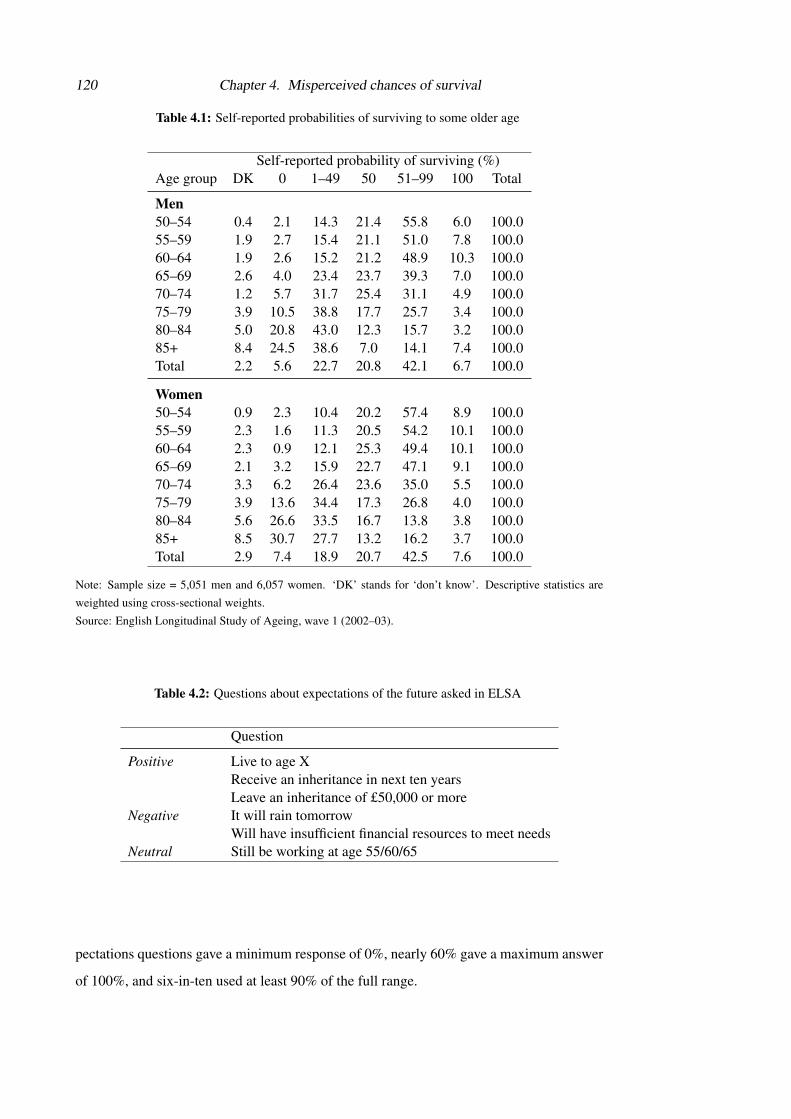
120 Chapter 4. Misperceived chances of survival
Table 4.1: Self-reported probabilities of surviving to some older age
Self-reported probability of surviving (%)Age group DK 0 1–49 50 51–99 100 Total
Men50–54 0.4 2.1 14.3 21.4 55.8 6.0 100.055–59 1.9 2.7 15.4 21.1 51.0 7.8 100.060–64 1.9 2.6 15.2 21.2 48.9 10.3 100.065–69 2.6 4.0 23.4 23.7 39.3 7.0 100.070–74 1.2 5.7 31.7 25.4 31.1 4.9 100.075–79 3.9 10.5 38.8 17.7 25.7 3.4 100.080–84 5.0 20.8 43.0 12.3 15.7 3.2 100.085+ 8.4 24.5 38.6 7.0 14.1 7.4 100.0Total 2.2 5.6 22.7 20.8 42.1 6.7 100.0
Women50–54 0.9 2.3 10.4 20.2 57.4 8.9 100.055–59 2.3 1.6 11.3 20.5 54.2 10.1 100.060–64 2.3 0.9 12.1 25.3 49.4 10.1 100.065–69 2.1 3.2 15.9 22.7 47.1 9.1 100.070–74 3.3 6.2 26.4 23.6 35.0 5.5 100.075–79 3.9 13.6 34.4 17.3 26.8 4.0 100.080–84 5.6 26.6 33.5 16.7 13.8 3.8 100.085+ 8.5 30.7 27.7 13.2 16.2 3.7 100.0Total 2.9 7.4 18.9 20.7 42.5 7.6 100.0
Note: Sample size = 5,051 men and 6,057 women. ‘DK’ stands for ‘don’t know’. Descriptive statistics are
weighted using cross-sectional weights.
Source: English Longitudinal Study of Ageing, wave 1 (2002–03).
Table 4.2: Questions about expectations of the future asked in ELSA
Question
Positive Live to age XReceive an inheritance in next ten yearsLeave an inheritance of £50,000 or more
Negative It will rain tomorrowWill have insufficient financial resources to meet needs
Neutral Still be working at age 55/60/65
pectations questions gave a minimum response of 0%, nearly 60% gave a maximum answer
of 100%, and six-in-ten used at least 90% of the full range.

4.3. Data 121
Figure 4.2: Self-reported expectations of surviving to age 75
Notes: Sample is all core sample members aged between 50 and 65.
Source: English Longitudinal Study of Ageing, wave 1 (2002–03).
4.3.2 Mortality outcomes
For the purposes of this paper, it is crucial that I can identify deaths among ELSA respond-
ents. Deaths among ELSA respondents are tracked through two methods. First, respondents
are asked for permission to link their survey responses to the National Health Service Cent-
ral Register (NHSCR), which is run by the Office for National Statistics. This register keeps
track of death registrations made with General Practitioners and also official death registra-
tions, including for those people who leave the UK health system. The vast majority of
ELSA respondents (95%) gave permission for their data to be linked to this register.
Second, ELSA respondents are asked to provide the name of an appropriate friend or
relative who can be contacted if the survey agency is unable to contact the original respond-
ent. These contacts are a second source of information about deaths among respondents.
We therefore have almost complete information about the mortality of ELSA respondents,
even if they have attrited from the survey.
Information from the NHSCR is currently available on deaths up to February 2013.
Up to that point, 5,246 ELSA respondents had died. This included 2,576 (22.6%) of the
original 11,391 core sample members. Of those sample members who were aged 65 and

122 Chapter 4. Misperceived chances of survival
under in the first wave of ELSA, 7.7% (or 478 individuals) had died.
4.3.3 Other covariates
I construct a number of other important covariates using responses from ELSA. The most
important of these are described here.
Education is defined based on the age that individuals left full-time education. Those
who left at (or before) the earliest legally allowable age (which varied across cohorts) are
defined as having ‘low’ education. Those who continued in education to age 19 or above
are defined as having ‘high’ education. The remainder are defined as ‘mid’ educated.
Numeracy is defined based on individuals’ responses to a series of increasingly com-
plex mathematical questions, which are based on everyday situations. I use the four-way
grouping that was originally presented by Banks and Oldfield (2007). The best numeracy
group, for example, includes those who were able to answer correctly a question requiring
understanding of compound interest in a bank account.
Income and wealth quintiles are defined within each five-year age band. The measure
of income used is total equivalised household income. The measure of wealth used is total
household net non-pension wealth – that is, the sum of wealth held in financial and physical
assets, housing and other property, less any outstanding (secured or unsecured) debts.
ELSA includes a wide range of measures of physical and mental health. I focus in
this paper on a subset of these. I include measures of whether or not a doctor has previ-
ously diagnosed specific health conditions (e.g. diabetes and cancer) and health behaviours
(smoking and drinking alcohol). I also include measures of cognitive functioning based on
individuals’ ability to recall items from a list of words (both immediately and with a delay).
I also use information about whether respondents’ parents are still alive and, if not, at what
age they died. Some ELSA respondents did not know whether or not their parents were still
alive – this was more common in the case of respondents’ fathers than mothers.
4.4 Evaluating self-reported survival probabilities
There are several related, but potentially slightly different, constructs that we might be in-
terested in as economic researchers hoping to understand economic behaviour. There are at
least five items of potential interest: (i) the individual’s stated subjective expectation; (ii) the
individual’s actual subjective expectation (i.e. that which she uses when making decisions);
(iii) the best objective estimate of her chance of survival, given her information set; (iv) the

4.4. Evaluating self-reported survival probabilities 123
best objective estimate of her chance of survival, given the researcher’s information set; (v)
her mortality outcome.
ELSA provides direct observations of (i) and (v). Using data on (v) for all sample
members, one can estimate (iv).10 Furthermore, to the extent that (i) is predictive of (v),
over and above the results of (iv), we can infer that (iii) and (iv) are not identical – that
is, respondents have some ‘private’ information that is not in the researchers’ information
set.11 I focus here on examining the relationship between (i), (iii), (iv) and (v). In Chapter
5 I demonstrate that reported expectations are predictive of economic behaviour – thus
suggesting that (i) conveys information about (ii).
4.4.1 Nature of responses
As has been found in other surveys asking questions of this type (see Gan, Hurd, and Mc-
Fadden (2005) for a discussion), there is a significant amount of bunching in subjective
survival expectations at focal point answers. For example, there are a surprisingly large
number of people reporting a 100% chance of surviving to age 75. This answer cannot be
an accurate reflection of any respondent’s true survival probability (given that they are all
at least ten years from age 75), and yet 8.1% of men and 9.8% of women aged 50–65 gave
this answer in wave 1 (as Table 4.3 shows).
People reporting 0% or 100% chances of survival appear to be demonstrating implaus-
ible levels of certainty about the future. Answers of 0% and 100% may be indicative of
some respondents not understanding the concept of probabilities and/or not understanding
the true risk they face. Clearly in reality there are not so many people who face exactly 0%
or 100% chances of survival.
There are also a large number of people who report a 50% chance of survival. Un-
like a response of 100%, 50% could reflect an individuals’ true chance of surviving to age
75. The fraction of people reporting this answer is high: 21.1% of men and 21.6% of wo-
men aged 50–65 reported that there was a 50:50 chance that they would survive to age 75.
Such answers could reflect individuals approximating appropriately in the face of consider-
able future uncertainty – indeed, respondents giving answers of (say) 47% or 51% may be
10Alternatively, one could use population life tables. However, these may not be ideal for two reasons. First,population life tables are typically period, rather than cohort, based – that is, they do not factor in expectedfuture improvements in life expectancy. Second, population life tables only distinguish between individuals onthe basis of sex – there are no more detailed, characteristic-specific official life tables available for England.
11Survey methodologists are likely to be interested in developing techniques to ensure that (iv) is as closeas possible to (iii).

124 Chapter 4. Misperceived chances of survival
Table 4.3: Reported chance of surviving to age 75
Percentage who reported...DK ps
75 = 0 ps75 = 50 ps
75 = 100 Mean N
Men
Education levelLow 1.5 3.5 23.3 8.7 58.7 1,340Mid 0.8 1.7 20.2 8.5 66.2 881High 2.0 1.3 16.9 5.7 65.4 501
Total 1.4 2.5 21.1 8.1 62.4 2,722
Numerical abilityWorst 8.7 4.5 25.5 11.8 57.9 1782 1.2 3.7 24.0 9.5 59.1 9433 0.4 2.0 19.9 7.5 64.5 948Best 1.0 1.0 17.5 5.7 65.1 653
Total 1.4 2.5 21.1 8.1 62.4 2,722
Women
Education levelLow 2.1 2.3 23.4 11.9 63.6 1,556Mid 0.9 1.4 21.8 8.5 66.6 1,162High 2.3 0.3 14.0 5.7 71.3 414
Total 1.7 1.7 21.6 9.8 65.7 3,132
Numerical abilityWorst 6.8 3.5 21.2 11.7 59.7 4442 0.9 1.9 22.8 10.6 65.2 1,6003 0.4 0.8 20.7 8.5 68.4 821Best 1.0 0.0 17.8 6.3 70.3 267
Total 1.7 1.7 21.6 9.8 65.7 3,132
Note: ‘DK’ stands for ‘don’t know’. ps75 stands for the self-reported probability of surviving to age 75. De-
scriptive statistics are weighted using cross-sectional weights.
Source: English Longitudinal Study of Ageing, wave 1 (2002–03).
providing spuriously precise answers.
What is of interest for many research questions is not the individuals’ true chances of
survival, but rather what individuals think are their chances of survival. Here I present ana-
lysis to provide some validation of individuals’ answers – trying to shed light on whether
they appear to understand the concept of probabilities and thus are able to provide mean-
ingful responses to questions of this sort.
Table 4.3 summarises the answers provided by those with different education and nu-
meracy levels. The prevalence of 0% and 100% responses is similar among men (10.6%)

4.4. Evaluating self-reported survival probabilities 125
and women (11.5%).12 However, it is clear that these focal point answers are much more
common among those with lower educational attainment and those with lower levels of
numeracy than the high educated and/or more numerate. For example, among men in the
lowest numeracy group, 16.3% reported 0% or 100%, compared to 6.7% of men with the
highest education levels – these figures are different from one another at the 1% signific-
ance level. There are also differences in the prevalence of 50% responses among more and
less numerate individuals. However, even among the most numerate men and women, a
significant minority give this answer (17.5% and 17.8%, respectively), suggesting that such
answers do not simply reflect a lack of understanding of the concept of probabilities.
Figure 4.3 shows what fraction of respondents reported a 0% or 100% chance of sur-
vival, split by the number of other 0% and/or 100% answers they gave to the other questions
about expectations of the future (see Table 4.2). This suggests that there is a correlation
(although not a perfect one) between the tendency to report focal answers on other expect-
ational questions and the tendency to report a focal answer when asked about chances of
survival. Around a third of men and women who gave focal answers to all the other ques-
tions they were asked also gave a focal answer about their survival chances. This compares
to less than three in one hundred of those who did not give any other focal answers.
4.4.2 How do expectations correlate with risk factors?
One test of the informational content of self-reported survival expectations is to examine
how expectations relate to known risk factors. A number of factors – both health-related
and socioeconomic – are known to be associated with lower chances of living to old age.
In the case of health risks – such as smoking (Lew and Garfinkel, 1987) and having various
pre-existing health conditions – there are well-established causal pathways between these
health behaviours or conditions and subsequent mortality. In the case of socioeconomic
characteristics, the causality is less clear, though much debated (Smith, 1998). It is of in-
terest to examine whether individuals’ subjective expectations display the same correlations
with individual characteristics as we know mortality outcomes do.
I present the results of multivariate analysis to assess which factors are most strongly
related to the self-reported expectation of surviving to age x (henceforth, psx), where x varies
depending on the age of the respondent at the time of interview.
I use data on psx from each of the first five waves of ELSA to estimate the regression
12I cannot reject that these figures are the same at standard levels of significance.

126 Chapter 4. Misperceived chances of survival
Figure 4.3: Whether report 0% or 100% chance of survival, by number of other focal answers given
Notes: Sample is all core sample members who responded to all expectations questions.
Source: English Longitudinal Study of Ageing, wave 1 (2002–03).
shown in Equation 4.1 using Ordinary Least Squares. The dependent variable takes values
between 0 and 100. The equation is estimated separately for men and women. age ∗wave
is a full set of interactions between dummy variables for each single year of age and each
wave of the data. This allows for average survival probabilities to differ between men and
women of different ages (and to change for each group over time), in the way that life table
mortality rates do. (For brevity, these coefficients are not reported.) X is a vector of other
individual characteristics that have been shown in other work to be correlated with survival.
(psx)it = β (ageit ∗waveit)+X
′itγ + εit (4.1)
The results of this regression are shown in Table 4.4 for men and Table 4.5 for wo-
men. Two alternative specifications are presented – one excluding self-rated health and one
including this. We might expect self-reported life expectancy and self-rated health to be
strongly correlated for a number of reasons. First, those who think their health is bad may
well not expect to live for that long. Second, those who are generally pessimistic may report
both poor current health and low chances of survival. On the other hand, there ought to be

4.4. Evaluating self-reported survival probabilities 127
an expectational component of psx that need not also manifest in self-rated current health.
Any relationship between psx and known mortality risk factors over and above self-rated
health is suggestive of psx containing an additional expectational component.
Table 4.4: Deviation of self-reported chance of survival from age/sex group average (men)
Objective measures Incl. SAHCoeff. Std error Coeff. Std error
Couple 0.997 (0.746) 1.092 (0.722)Education level (rel. to mid)
Low –1.095* (0.658) –0.654 (0.636)High 0.185 (0.763) 0.094 (0.739)
Income quintile (rel. to quintile 3)Lowest –0.876 (0.761) –0.545 (0.740)2 0.310 (0.662) 0.391 (0.643)4 0.549 (0.623) 0.460 (0.603)Highest –0.017 (0.675) –0.040 (0.656)
Wealth quintile (rel. to quintile 3)Lowest 0.844 (0.909) 2.210** (0.879)2 0.230 (0.732) 0.660 (0.712)4 –0.036 (0.677) –0.289 (0.653)Highest 0.396 (0.749) –0.126 (0.726)
Working 3.064*** (0.641) 1.199* (0.620)Smoking (rel. to non-smoker)
Ex-occasional smoker –2.994** (1.286) –2.672** (1.244)Ex-regular smoker –1.645*** (0.631) –1.096* (0.609)Ex-smoker (DK frequency) –2.628** (1.331) –2.102 (1.306)Current smoker –8.177*** (0.875) –6.563*** (0.847)
Frequency of alcohol consumption (rel. to once or twice a month)At least 3-4 days a week –0.131 (0.790) –0.827 (0.770)Once or twice a week 0.110 (0.758) –0.071 (0.741)A few times a year –0.910 (0.968) –0.214 (0.941)Not at all –2.539** (1.209) –1.380 (1.178)
Doctor diagnosed conditionsHypertension –2.293*** (0.558) –0.936* (0.546)Heart condition –3.446*** (0.988) –1.843* (0.957)Angina –4.279*** (1.019) –2.276** (0.979)Stroke –2.146 (1.485) –0.215 (1.440)Diabetes –3.418*** (0.950) –1.334 (0.920)Asthma –0.571 (0.872) 1.053 (0.850)Lung disease –6.974*** (1.239) –3.437*** (1.203)Cancer –6.450*** (1.134) –4.279*** (1.099)Arthritis –1.843*** (0.614) 0.118 (0.603)Osteoporosis –0.976 (2.158) 0.620 (2.140)Alzheimer’s –5.580 (7.387) –6.065 (7.136)Dementia –4.150 (3.979) –1.058 (3.886)Parkinson’s –2.126 (3.001) 2.137 (2.938)

128 Chapter 4. Misperceived chances of survival
Table 4.4 – continued from previous pageObjective measures Incl. SAHCoeff. Std error Coeff. Std error
Psychological problems –3.214*** (0.986) –1.379 (0.956)Immediate recall – no. words –0.047 (0.170) –0.177 (0.165)Delayed recall – no. words 0.523*** (0.151) 0.350** (0.147)Age father died (rel. to 60–64)
<50 1.577 (1.587) 1.874 (1.528)50–59 –0.060 (1.348) 0.295 (1.298)65–69 0.824 (1.318) 0.759 (1.277)70–74 2.818** (1.257) 2.809** (1.225)75–79 4.281*** (1.228) 4.297*** (1.195)80–84 4.593*** (1.252) 4.352*** (1.205)85+ 8.022*** (1.283) 7.923*** (1.256)Still alive 8.635*** (1.296) 8.378*** (1.260)Don’t know 1.065 (1.547) 1.390 (1.497)
Age mother died (rel. to 60–64)<50 1.623 (1.755) 1.803 (1.697)50–59 1.351 (1.691) 1.069 (1.637)65–69 3.642** (1.694) 3.599** (1.657)70–74 2.792* (1.533) 2.803* (1.493)75–79 2.499* (1.509) 2.080 (1.475)80–84 3.307** (1.446) 2.983** (1.416)85+ 6.391*** (1.419) 5.932*** (1.380)Still alive 5.091*** (1.386) 4.549*** (1.348)Don’t know 4.449** (1.905) 4.705** (1.835)
Non-white –0.883 (1.665) –0.115 (1.583)Self-rated health (rel. to good)
Excellent 9.634*** (0.696)Very good 4.731*** (0.488)Fair –6.421*** (0.666)Poor –14.672*** (1.096)
Sample size 17,927 17,927
Notes: Results are from an OLS regression. *** denotes that the effect is significantly different from zero at
the 1% level, ** at the 5% level, * at the 10% level. Standard errors are clustered at the individual level.
Source: English Longitudinal Study of Ageing, waves 1–6.
I start by discussing the results when self-rated health is not included. For both men and
women, there is a strong correlation between health and health behaviours and expectations
of survival. In contrast, most of the socioeconomic variables are not significant. This is des-
pite the fact that there are strong unconditional correlations between socioeconomic status
and survival expectations.13 The fact that the correlation between socioeconomic status and
survival expectations is attenuated by including controls for health and health behaviours
indicates that the raw correlation is largely driven by those with lower levels of education,
13For brevity, these univariate descriptives are not reported.

4.4. Evaluating self-reported survival probabilities 129
income and/or wealth being in worse health and more likely to engage in dangerous health
behaviours – in particular, smoking.
Only the following significant differences remain between socioeconomic status and
survival expectations. Men in the lowest education group report lower than average life
expectancies, with an average self-reported chance of surviving to age 75 that is 1.1 per-
centage points lower than mid-educated men of the same age at the same point in time (all
else equal). There is also a significant difference between those who are in work compared
to non-workers. Men who are working report average psx that is 3.1 percentage points higher
than non-workers, while for women the difference is 2.4 percentage points.
Among men, but not among women, former smokers report significantly lower chances
of survival than those who have never smoked. For example, men who used to smoke regu-
larly report psx that is on average 1.6 percentage points lower than non-smokers. This com-
pares to a difference of 8.2 percentage points for current smokers, suggesting that former
smokers believe their survival chances are much closer to those of non-smokers than to
those of current smokers. (However, as I show in Section 4.4.4, subsequent deaths suggest
that former male and female smokers in fact have death rates equidistant between those of
smokers and non-smokers, all else equal.)
The relationships between many specific health diagnoses and psx are significant after
controlling for other characteristics and conditions. It is men and women who have pre-
viously been diagnosed with lung disease or cancer who, all else equal, have the lowest
expectations of survival. For example, women who have been diagnosed with cancer report
psx that is on average 3.9 percentage points lower than those who have not been diagnosed
with any of the conditions listed.
Finally, parents’ age at death is significantly related to respondents’ survival expecta-
tions, even after controlling for objective measures of respondents’ current health. In par-
ticular, those whose mother and/or father survived to age 70+ (for men) or 80+ (for women)
report significantly higher average psx than those whose parents died in their early sixties.
Comparing the coefficients in the two alternative specifications shown in Tables 4.4
and 4.5 provides some interesting insights. As would be expected, adding controls for
self-rated health attenuates the coefficients on the objective health conditions. That is, the
difference in psx between those with and without (for example) a diagnosis of lung disease,
is smaller when I also control for individuals’ perceived current general health than when

130 Chapter 4. Misperceived chances of survival
I do not. In contrast, the coefficients on parents’ age at death (and, to a lesser extent, past
smoking behaviour) are little changed by the inclusion of self-rated health – suggesting that
these measures contain information about expected future longevity that is not captured by
self-reported current health.
Table 4.5: Deviation of self-reported chance of survival from age/sex group average (women)
Objective measures Incl. SAHCoeff. Std error Coeff. Std error
Couple 0.915 (0.558) 1.083** (0.541)Education level (rel. to mid)
Low –0.268 (0.552) 0.091 (0.535)High 0.980 (0.688) 0.607 (0.664)
Income quintile (rel. to quintile 3)Lowest –0.466 (0.607) –0.565 (0.591)2 –0.244 (0.551) –0.156 (0.539)4 0.341 (0.550) 0.382 (0.542)Highest –0.080 (0.613) –0.332 (0.598)
Wealth quintile (rel. to quintile 3)Lowest –0.829 (0.750) 0.060 (0.730)2 –0.523 (0.603) –0.184 (0.586)4 0.299 (0.581) –0.034 (0.568)Highest 0.429 (0.665) –0.169 (0.647)
Working 2.419*** (0.544) 0.849 (0.529)Smoking (rel. to non-smoker)
Ex-occasional smoker –0.401 (0.920) 0.079 (0.898)Ex-regular smoker –0.341 (0.542) –0.022 (0.526)Ex-smoker (DK frequency) –1.630 (1.353) –1.146 (1.325)Current smoker –6.893*** (0.744) –5.731*** (0.719)
Frequency of alcohol consumption (rel. to once or twice a month)At least 3-4 days a week 0.395 (0.659) –0.020 (0.640)Once or twice a week 0.197 (0.608) –0.073 (0.589)A few times a year –1.074* (0.641) –0.698 (0.623)Not at all –1.725** (0.817) –0.632 (0.789)
Doctor diagnosed conditionsHypertension –2.617*** (0.484) –1.499*** (0.471)Heart condition –2.217*** (0.846) –1.244 (0.821)Angina –3.263*** (1.006) –1.520 (0.982)Stroke –0.402 (1.329) 1.381 (1.284)Diabetes –1.425 (0.952) 0.337 (0.928)Asthma –2.538*** (0.682) –1.157* (0.668)Lung disease –3.803*** (1.159) –1.486 (1.115)Cancer –3.886*** (0.852) –2.585*** (0.824)Arthritis –1.464*** (0.479) 0.519 (0.472)Osteoporosis –1.471* (0.797) 0.302 (0.777)Alzheimer’s –3.301 (7.191) –2.734 (7.001)

4.4. Evaluating self-reported survival probabilities 131
Table 4.5 – continued from previous pageObjective measures Incl. SAHCoeff. Std error Coeff. Std error
Dementia –3.591 (4.386) –1.784 (4.337)Parkinson’s –3.605 (5.150) 0.290 (4.738)Psychological problems –2.174*** (0.726) –0.721 (0.697)
Immediate recall – no. words 0.183 (0.148) 0.074 (0.144)Delayed recall – no. words 0.511*** (0.132) 0.356*** (0.130)Age father died (rel. to 60–64)
<50 0.648 (1.297) 0.743 (1.256)50–59 0.989 (1.155) 1.084 (1.113)65–69 –0.790 (1.151) –0.480 (1.102)70–74 1.857* (1.062) 1.715* (1.016)75–79 3.398*** (1.070) 3.399*** (1.034)80–84 2.931*** (1.090) 2.860*** (1.048)85+ 4.883*** (1.093) 4.779*** (1.051)Still alive 4.058*** (1.109) 3.678*** (1.067)Don’t know 0.662 (1.258) 1.053 (1.222)
Age mother died (rel. to 60–64)<50 1.988 (1.566) 2.186 (1.530)50–59 –2.141 (1.529) –2.043 (1.484)65–69 –1.540 (1.408) –1.304 (1.365)70–74 –0.383 (1.313) –0.276 (1.268)75–79 0.705 (1.278) 0.707 (1.239)80–84 2.732** (1.215) 2.884** (1.176)85+ 7.286*** (1.169) 7.361*** (1.137)Still alive 5.867*** (1.155) 5.938*** (1.120)Don’t know 0.782 (1.553) 0.983 (1.516)
Non-white –7.682*** (1.660) –6.253*** (1.625)Self-rated health (rel. to good)
Excellent 9.579*** (0.590)Very good 5.090*** (0.434)Fair –4.761*** (0.564)Poor –10.807*** (0.989)
Sample size 21,843 21,843
Notes: Results are from an OLS regression. *** denotes that the effect is significantly different from zero at
the 1% level, ** at the 5% level, * at the 10% level.
The analysis presented in this section suggests that self-reported survival expectations
do correlate with known risk factors. Furthermore, it appears that this measure conveys
information about future chances of survival that are not captured by measures of current
health (either objectively measured or self-reported).
4.4.3 Comparing self-reports to life table values
Assuming that individuals’ expectations of surviving to a given age, x, reflect the probability
of a binomial random variable taking the value 1, we would expect the number of survivors
132 Chapter 4. Misperceived chances of survival
to age x in the population to be equal to ∑ psx. Thus the average expected survival rate
would be ∑ps
xn , which would be the value given by a cohort-specific life table for the relevant
population.
Official life tables available for England – produced by the Office for National Statistics
– are period-specific. That is, they estimate the probability of surviving to a particular future
age based on the mortality experience of current older individuals, rather than factoring in
potential future improvements in life expectancy. There are therefore three weaknesses in
comparing ELSA respondents’ self-reported expectations of survival to life table values.
First, the period life table values are based on mortality among individuals of different ages
at a point in time – therefore, they do not factor in potential improvements in survival rates
across cohorts. Second, the population to which the life table applies may not be the same
as the sample captured by ELSA – for example, because ELSA is representative only of the
household population and not those in institutions, who are likely to have lower survival
probabilities. Third, there is considerable heterogeneity in individual survival probabilities
that cannot be gleaned from these population life tables, which distinguish only between
men and women.
Despite these weaknesses there are some interesting lessons to be learned from com-
paring ELSA responses to life table figures, which I do in this subsection. In the next
subsection I then examine how survival expectations relate to outcomes for the same group
of people, which overcomes many of the concerns just mentioned.
Bearing the aforementioned caveats in mind, Figure 4.4 compares survival probabilit-
ies taken from contemporaneous life tables to average self-reported expectations of survival
for men (left-hand panel) and women (right-hand panel). Different age groups are asked
about survival to different target ages; therefore four pairs of lines are shown in each panel.
This figure pools data from all six waves of ELSA and compares the self-reported figures
to the equivalent figures from the contemporaneous population life table (e.g. self-reported
answers in wave 1 are compared to the 2002-based period life table).
It appears that individuals, on average, underestimate their chances of surviving to
younger ages (75 and 80) but over-estimate their chances of surviving to ages 85 and 90.
The under-estimate at younger ages is larger for women than men, while the overestimate
at older ages is larger for men than women. The apparent underestimate at younger ages
would be exacerbated if we took into account future improvements in longevity, while the
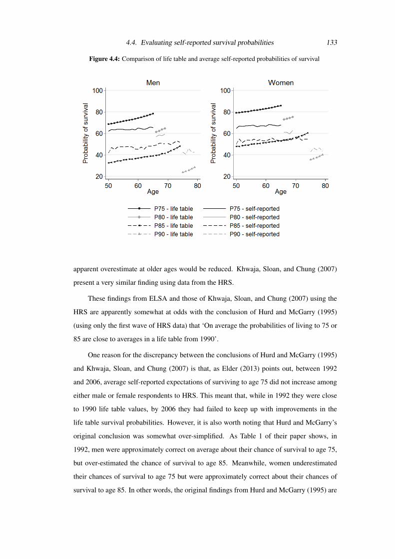
4.4. Evaluating self-reported survival probabilities 133
Figure 4.4: Comparison of life table and average self-reported probabilities of survival
apparent overestimate at older ages would be reduced. Khwaja, Sloan, and Chung (2007)
present a very similar finding using data from the HRS.
These findings from ELSA and those of Khwaja, Sloan, and Chung (2007) using the
HRS are apparently somewhat at odds with the conclusion of Hurd and McGarry (1995)
(using only the first wave of HRS data) that ‘On average the probabilities of living to 75 or
85 are close to averages in a life table from 1990’.
One reason for the discrepancy between the conclusions of Hurd and McGarry (1995)
and Khwaja, Sloan, and Chung (2007) is that, as Elder (2013) points out, between 1992
and 2006, average self-reported expectations of surviving to age 75 did not increase among
either male or female respondents to HRS. This meant that, while in 1992 they were close
to 1990 life table values, by 2006 they had failed to keep up with improvements in the
life table survival probabilities. However, it is also worth noting that Hurd and McGarry’s
original conclusion was somewhat over-simplified. As Table 1 of their paper shows, in
1992, men were approximately correct on average about their chance of survival to age 75,
but over-estimated the chance of survival to age 85. Meanwhile, women underestimated
their chances of survival to age 75 but were approximately correct about their chances of
survival to age 85. In other words, the original findings from Hurd and McGarry (1995) are

134 Chapter 4. Misperceived chances of survival
actually more consistent with my findings and those of Khwaja, Sloan, and Chung (2007)
than they might first appear.
One interpretation of Figure 4.4 is that respondents simply have a tendency to report
answers to probabilistic questions that are ‘too close’ to 50%. Certainly the figure suggests
subjective survival expectations are most ‘accurate’ when the ‘true’ probability is close to
50%. However, if these responses simply reflected a general bias in responding to questions
of this type, we might expect it also to affect responses to other questions about expectations
of the future. In practice, this tendency to report answers that are too close to 50% is not
evident in Figure 4.5, which compares actual and self-reported chances of rain.14
The figure shows that the average individual self-reported chance of rain (among those
individuals interviewed in the same region and in the same month) is correlated with the
actual historic average. The line of best fit through the mean self-reported probabilities
shown in Figure 4.5 has a slope of 0.6 and an R2 of 21.9%. However, whereas the ‘true’
chance of rain was below 50% for virtually all groups, respondents’ average answers were
above 50% in most cases.
Unfortunately, at the moment it is only possible to match historic rainfall data to ELSA
respondents at a very coarse geographic level. A priority for future work, which I am
currently pursuing, is to match rainfall probabilities at a finer geographic level to allow for
a more robust assessment of my assertion that individuals do not appear to suffer merely
from a general tendency to report answers that are too close to 50%.
If the self-reported survival expectations in ELSA reflect individuals’ true perceptions
of their chances of survival (and if younger individuals respond in a similar way in future to
current older individuals) then it suggests that ELSA respondents’ self-perceived survival
curves are flatter than the life table survival curves. That is, ELSA respondents perceive
that they face greater uncertainty about their future age of death than the life tables would
suggest they do. This is perhaps somewhat surprising if (as seems likely) individuals know
more about their own health and behaviour than is conveyed by their age and sex alone.
Given this additional information, we would expect them to face less, not more, uncertainty
about their chances of survival.
This conclusion that individuals believe they face flatter survival curves is reinforced
14The historic average chance of rain is calculated based on the fraction of days in a given month, in a givenregion on which there was at least 1mm of rain – using data on rainfall collected between 1961 and 2013. Ifocus here on expectations of rain because it is not possible to construct an estimate of the true chance of anyof the other outcomes that are asked about.

4.4. Evaluating self-reported survival probabilities 135
Figure 4.5: Comparing historic average chances of rain to mean self-reported probabilities
Notes: Mean self-reported chances are calculated across individuals interviewed in the same month and in the
same region. These are compared to the average of the proportion of days in that month in that region that there
has been at least 1mm of rain, based on data from 1961– 2013.
Source: English Longitudinal Study of Ageing, wave 1 (2002–03); Met Office rainfall data.
by evidence from a sub-group of ELSA respondents – those aged under 70 in waves 3–6 –
who were asked a second question about their survival expectations. They were also asked
about their expectations of surviving to age 85. As shown in Figure 4.4, this subgroup not
only under-estimate the chances of surviving to 75/80 but also over-estimate the chances
of surviving to age 85. For this group, the combination of the two answers potentially
provides information about the shape of the individuals’ perceived survival curve. Section
4.5 presents estimates of the shape of these underlying survival curves. Section 4.6 then
shows what the implications of such flat survival curves would be for economic behaviour
in a simple life-cycle model.
4.4.4 Validating survival expectations using outcomes
The previous subsection compared self-reported survival expectations to life table values.
However, as noted above, there are a number of potential drawbacks to using life tables
as the point of reference. Therefore, it is also worth looking at how expectations relate to
mortality outcomes for the same sample.

136 Chapter 4. Misperceived chances of survival
One test of the value of self-reported survival expectations is whether or not they pre-
dict actual mortality outcomes and – as a stronger test – whether self-reported survival
expectations predict outcomes over and above what would be predicted from objectively
measured characteristics. With ten years of mortality follow-up since the first wave of
ELSA, we now have considerable information on actual outcomes to be able to examine
self-reported measures in this way.
In wave 1 of ELSA (collected between spring 2002 and spring 2003), those aged under
66 were asked about their chances of surviving to age 75. With the mortality data we now
have (which covers the period up to February 2013), 511 of the original 6,010 wave 1 sample
members who reported an expectation of surviving to age 75, had (or would have, if they
survived) reached age 75. For this subgroup, I can compare their answers in wave 1 to their
outcomes for the exact risk about which they were asked (namely, survival to age 75).15 For
the others, I can only look at their survival over a fixed time window (up to February 2013 at
the latest) and, therefore, have to make the assumption that this outcome is correlated with
survival to age 75. This is true for commonly used survival curves, such as the Weibull or
Gompertz distributions.
Surviving to age 75: expectations and outcomes
Figure 4.6 shows the relationship between baseline self-reported expectations of dying be-
fore age 75 and actual deaths before that age. Owing to small sample sizes, I group together
quite wide ranges of baseline answers. The ‘dots’ show the mean of (1− ps75) reported
by the group in wave 1, while the ‘bars’ show the actual fraction who died before reach-
ing age 75. There is clearly a correlation between baseline expectations and subsequent
outcomes. However, on average individuals were pessimistic – that is, for all but the bot-
tom two groups, the actual proportion dying was lower than the original average expected
death rate. This is in keeping with the analysis above comparing to life table values, which
also suggested that respondents were pessimistic about their chances of surviving to age 75.
There appears, however, to be little correlation between actual survival rate and self-reported
expectations among those who reported less than a 40% chance of dying at baseline. How-
ever, there is still only a small sample for whom we can compare the baseline expectation
to the actual outcome that was asked about.
15None of the respondents who were asked about survival to older ages (e.g. 80 or 85) would have reachedthat age by February 2013 so I cannot compare expectations and outcomes for any of these older ages.

4.4. Evaluating self-reported survival probabilities 137
Figure 4.6: Fraction of respondents dying by age 75, by self-reported chances of dying before age75
Notes: Sample is core sample members who were aged 65 and under in wave 1 and who (or would have, had
they survived) reached age 75 by February 2013. Those who did not report their expected chance of survival to
age 75 in wave 1 are excluded.
Source: English Longitudinal Study of Ageing, wave 1 (2002–03).
Correlation between survival expectations and 10-year mortality
For the full sample of wave 1 respondents, I can compare 10-year mortality to original self-
reported expectations of survival. This is done in Figure 4.7, which shows what fraction
of respondents had died within ten years of their wave 1 interview, split by their reported
chances of dying by age 75 (i.e. 1− ps75) in wave 1.16 This figure is reassuring about the
value of the information conveyed by self-reported chances of survival. In particular, it
is worth noting that death rates among those who reported a 50:50 chance of survival are
similar to those for people reporting (non-focal) answers somewhat higher or lower than
this, suggesting that the 50% response may not simply reflect ‘noise’. Similarly, those who
report 100% chances of dying do have the highest death rates. However, Figure 4.7 suggests
that those who report the lowest probabilities of dying (less than 10%) may misperceive
their true chances of survival, since more of them died than did those who reported slightly
higher probabilities.
16The groupings shown in Figure 4.7 are chosen to avoid sample sizes of less than 30.

138 Chapter 4. Misperceived chances of survival
Figure 4.7: Fraction of respondents dying within ten years, by self-reported chances of dying byage 75
Notes: Sample is all core sample members aged 65 and under in wave 1 who responded to the question about
expected survival to age 75. Sample size = 6,010.
Source: English Longitudinal Study of Ageing, wave 1 (2002–03).
This raw correlation suggests that individuals’ expectations are correlated with their
subsequent outcomes and this is reassuring evidence that these answers convey meaningful
information. However, it is also interesting to ask whether self-reported survival expecta-
tions are predictive of subsequent survival over and above other observed characteristics at
baseline. To do this, I estimate equations of the following form for wave 1 sample members
aged 50–65, using a probit model.
Di,t+10 = X′itβ +ηit (4.2)
where Di,t+10 is a variable taking the value 1 if the individual dies within ten years of their
wave 1 interview and 0 otherwise, and X is a vector of covariates, which differs across
specifications. This model is estimated separately for men and women.
Results are presented in Tables 4.6 and 4.7 for men and women, respectively. Specific-
ation (1) includes only self-reported expectations of survival, specification (2) adds other
observed risk factors from wave 1 (including a full set of age dummies, which are not

4.4. Evaluating self-reported survival probabilities 139
reported in the table), and specification (3) adds a measure of baseline self-rated general
health.
Table 4.6: How well does self-reported life expectancy predict 10-year mortality? (men)
(1) (2) (3)Marg. effect Marg. effect Marg. effect(Std error) (Std error) (Std error)
ps75 –0.1445*** –0.0615*** –0.0421*
(0.0224) (0.0217) (0.0223)Couple –0.0149 –0.0170
(0.0136) (0.0135)Education level (rel. to mid)
Low –0.0113 –0.0114(0.0138) (0.0138)
High –0.0691*** –0.0677***(0.0151) (0.0151)
Income quintile (rel. to quintile 3)Lowest –0.0064 –0.0073
(0.0176) (0.0177)2 0.0015 –0.0025
(0.0174) (0.0173)4 –0.0066 –0.0088
(0.0171) (0.0171)Highest –0.0140 –0.0154
(0.0184) (0.0183)Wealth quintile (rel. to quintile 3)
Lowest 0.0333* 0.0280(0.0193) (0.0193)
2 –0.0016 –0.0063(0.0167) (0.0167)
4 –0.0129 –0.0148(0.0170) (0.0170)
Highest –0.0084 –0.0087(0.0186) (0.0188)
Working –0.0443*** –0.0327**(0.0135) (0.0139)
Smoking (rel. to non-smoker)Ex-occasional smoker 0.0073 0.0092
(0.0250) (0.0257)Ex-regular smoker 0.0453*** 0.0431***
(0.0127) (0.0127)Ex-smoker (DK frequency) –0.0196 –0.0203
(0.0197) (0.0197)Current smoker 0.0757*** 0.0725***
(0.0160) (0.0160)Frequency of alcohol consumption (rel. to once or twice a month)
At least 3-4 days a week 0.0188 0.0206
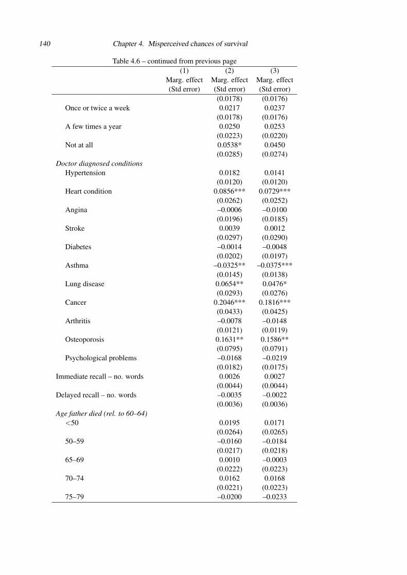
140 Chapter 4. Misperceived chances of survival
Table 4.6 – continued from previous page(1) (2) (3)
Marg. effect Marg. effect Marg. effect(Std error) (Std error) (Std error)
(0.0178) (0.0176)Once or twice a week 0.0217 0.0237
(0.0178) (0.0176)A few times a year 0.0250 0.0253
(0.0223) (0.0220)Not at all 0.0538* 0.0450
(0.0285) (0.0274)Doctor diagnosed conditions
Hypertension 0.0182 0.0141(0.0120) (0.0120)
Heart condition 0.0856*** 0.0729***(0.0262) (0.0252)
Angina –0.0006 –0.0100(0.0196) (0.0185)
Stroke 0.0039 0.0012(0.0297) (0.0290)
Diabetes –0.0014 –0.0048(0.0202) (0.0197)
Asthma –0.0325** –0.0375***(0.0145) (0.0138)
Lung disease 0.0654** 0.0476*(0.0293) (0.0276)
Cancer 0.2046*** 0.1816***(0.0433) (0.0425)
Arthritis –0.0078 –0.0148(0.0121) (0.0119)
Osteoporosis 0.1631** 0.1586**(0.0795) (0.0791)
Psychological problems –0.0168 –0.0219(0.0182) (0.0175)
Immediate recall – no. words 0.0026 0.0027(0.0044) (0.0044)
Delayed recall – no. words –0.0035 –0.0022(0.0036) (0.0036)
Age father died (rel. to 60–64)<50 0.0195 0.0171
(0.0264) (0.0265)50–59 –0.0160 –0.0184
(0.0217) (0.0218)65–69 0.0010 –0.0003
(0.0222) (0.0223)70–74 0.0162 0.0168
(0.0221) (0.0223)75–79 –0.0200 –0.0233

4.4. Evaluating self-reported survival probabilities 141
Table 4.6 – continued from previous page(1) (2) (3)
Marg. effect Marg. effect Marg. effect(Std error) (Std error) (Std error)
(0.0208) (0.0209)80–84 0.0331 0.0303
(0.0245) (0.0245)85+ 0.0441 0.0397
(0.0275) (0.0274)Still alive 0.0368 0.0340
(0.0266) (0.0265)Don’t know –0.0310 –0.0355
(0.0280) (0.0274)Age mother died (rel. to 60–64)
<50 0.0020 0.0034(0.0313) (0.0307)
50–59 –0.0253 –0.0238(0.0272) (0.0266)
65–69 0.0322 0.0326(0.0320) (0.0313)
70–74 0.0196 0.0239(0.0284) (0.0280)
75–79 –0.0042 –0.0007(0.0265) (0.0260)
80–84 0.0149 0.0181(0.0269) (0.0264)
85+ 0.0084 0.0112(0.0275) (0.0270)
Still alive –0.0089 –0.0050(0.0240) (0.0235)
Don’t know –0.0407 –0.0383(0.0445) (0.0444)
Non-white –0.0931** –0.0901**(0.0410) (0.0413)
Self-rated health (rel. to good)Excellent –0.0335**
(0.0161)Very good –0.0077
(0.0145)Fair 0.0007
(0.0166)Poor 0.0866***
(0.0315)Sample size 2,596 2,596 2,596R2 0.026 0.202 0.213
Notes: Results are from a probit regression. *** denotes that the effect is significantly different from zero at
the 1% level, ** at the 5% level, * at the 10% level.

142 Chapter 4. Misperceived chances of survival
Table 4.7: How well does self-reported life expectancy predict 10-year mortality? (women)
(1) (2) (3)Marg. effect Marg. effect Marg. effect(Std error) (Std error) (Std error)
ps75 –0.0669*** –0.0146 –0.0062
(0.0168) (0.0164) (0.0164)Couple 0.0006 0.0009
(0.0095) (0.0094)Education level (rel. to mid)
Low –0.0040 –0.0046(0.0091) (0.0091)
High 0.0236 0.0277(0.0179) (0.0184)
Income quintile (rel. to quintile 3)Lowest –0.0093 –0.0084
(0.0130) (0.0132)2 0.0026 –0.0007
(0.0135) (0.0133)4 –0.0074 –0.0083
(0.0137) (0.0137)Highest –0.0115 –0.0134
(0.0144) (0.0143)Wealth quintile (rel. to quintile 3)
Lowest 0.0179 0.0157(0.0147) (0.0143)
2 0.0031 0.0027(0.0131) (0.0128)
4 –0.0105 –0.0087(0.0126) (0.0126)
Highest –0.0129 –0.0090(0.0131) (0.0134)
Working –0.0173* –0.0105(0.0097) (0.0098)
Smoking (rel. to non-smoker)Ex-occasional smoker 0.0106 0.0100
(0.0183) (0.0184)Ex-regular smoker 0.0160 0.0156
(0.0098) (0.0099)Ex-smoker (DK frequency) 0.0152 0.0102
(0.0257) (0.0241)Current smoker 0.0318*** 0.0288**
(0.0116) (0.0114)Frequency of alcohol consumption (rel. to once or twice a month)
At least 3-4 days a week 0.0104 0.0132(0.0138) (0.0137)
Once or twice a week 0.0071 0.0111(0.0126) (0.0126)

4.4. Evaluating self-reported survival probabilities 143
Table 4.7 – continued from previous page(1) (2) (3)
Marg. effect Marg. effect Marg. effect(Std error) (Std error) (Std error)
A few times a year 0.0094 0.0086(0.0133) (0.0130)
Not at all 0.0344** 0.0304*(0.0175) (0.0166)
Doctor diagnosed conditionsHypertension –0.0047 –0.0081
(0.0086) (0.0084)Heart condition 0.0254 0.0220
(0.0203) (0.0195)Angina 0.0207 0.0096
(0.0220) (0.0196)Stroke 0.0490 0.0308
(0.0350) (0.0306)Diabetes 0.0212 0.0095
(0.0210) (0.0187)Asthma 0.0014 –0.0051
(0.0117) (0.0110)Lung disease 0.0606** 0.0486**
(0.0245) (0.0227)Cancer 0.0913*** 0.0826***
(0.0232) (0.0221)Arthritis 0.0034 –0.0062
(0.0087) (0.0087)Osteoporosis –0.0130 –0.0198
(0.0147) (0.0131)Psychological problems 0.0213 0.0144
(0.0138) (0.0130)Immediate recall – no. words –0.0027 –0.0020
(0.0033) (0.0033)Delayed recall – no. words –0.0009 –0.0009
(0.0028) (0.0028)Age father died (rel. to 60–64)
<50 –0.0137 –0.0112(0.0231) (0.0230)
50–59 –0.0282 –0.0276(0.0194) (0.0192)
65–69 –0.0097 –0.0097(0.0205) (0.0202)
70–74 –0.0376** –0.0349**(0.0176) (0.0175)
75–79 –0.0250 –0.0246(0.0184) (0.0181)
80–84 –0.0235 –0.0233(0.0195) (0.0192)

144 Chapter 4. Misperceived chances of survival
Table 4.7 – continued from previous page(1) (2) (3)
Marg. effect Marg. effect Marg. effect(Std error) (Std error) (Std error)
85+ –0.0195 –0.0171(0.0216) (0.0216)
Still alive –0.0326* –0.0295(0.0193) (0.0193)
Don’t know –0.0169 –0.0180(0.0273) (0.0265)
Age mother died (rel. to 60–64)<50 –0.0002 –0.0063
(0.0315) (0.0305)50–59 –0.0020 0.0007
(0.0281) (0.0281)65–69 –0.0592*** –0.0588***
(0.0221) (0.0218)70–74 –0.0363 –0.0359
(0.0224) (0.0222)75–79 –0.0256 –0.0249
(0.0233) (0.0231)80–84 –0.0358 –0.0326
(0.0225) (0.0226)85+ –0.0357 –0.0335
(0.0231) (0.0231)Still alive –0.0405* –0.0407*
(0.0210) (0.0208)Don’t know –0.0460 –0.0454
(0.0333) (0.0332)Non-white 0.0003 –0.0090
(0.0281) (0.0287)Self-rated health (rel. to good)
Excellent –0.0171(0.0107)
Very good 0.0025(0.0096)
Fair 0.0392***(0.0137)
Poor 0.0769***(0.0271)
Sample size 2,968 2,968 2,968R2 0.013 0.158 0.176
Notes: Results are from a probit regression. *** denotes that the effect is significantly different from zero at
the 1% level, ** at the 5% level, * at the 10% level.
The first specification confirms that ps75 does predict subsequent mortality. For ex-
ample, for women, each 10 percentage point increase in ps75 is associated with a 0.67 per-
centage point reduction in the chance of dying within ten years. The 10-year mortality

4.4. Evaluating self-reported survival probabilities 145
rate among this sample of women was 5.5%. However, the pseudo R2 for this specifica-
tion suggests that self-reported expectations of survival to age 75 explain only 1.3% of the
variation in 10-year survival probabilities. In other words, while ps75 is correlated with out-
comes, there is a significant amount of variation in survival chances that is not captured by
individuals’ expectations.
Among men, the relationship between expectations and outcomes is stronger than
among women, with a 10 percentage point increase in ps75 being associated with a 1.4 per-
centage point decrease in the chance of dying within ten years. The 10-year mortality rate
among this sample of men was 9.5%. The R2 suggests that self-reported expectations ex-
plain 2.6% of the variation in outcomes among men.
Adding in controls for other observed characteristics (including age dummies) in-
creases the R2 significantly and reduces the marginal effect for the self-reported expecta-
tions to less than half its previous value for men and less than a quarter for women. For
women, adding these other variables also causes the marginal effect of ps75 to become insig-
nificant, suggesting that women’s own survival expectations have no significant explanatory
power for future survival over and above the other observed characteristics.
Finally, adding self-rated current health reduces the marginal effect of self-reported
survival further. However, for men, ps75 continues to be significant. This suggests that,
for men, ps75 captures both an expectational component that is not captured by other self-
reported indicators of current health, and a degree of individual heterogeneity in survival
chances that cannot be picked up by the observed characteristics considered here. In other
words, men appear to have ‘private’ information about their chances of surviving that are
not conveyed by their observed characteristics or by their self-rated current health.
4.4.5 Summary
This section has shown that individuals are willing and able to answer questions about
their expectations of survival and that these answers are meaningful, in the sense of being
correlated with known risk factors and subsequent outcomes. I have also presented evidence
to suggest that individuals underestimate their chances of surviving to younger ages but
overestimate the chances of survival to older ages – and that this is not merely driven by a
tendency to report answers that are too close to 50% when asked probabilistic questions.
A further test of the validity of self-reported survival expectations is to examine
whether they actually predict behaviour in the way we would expect. Chapter 5 presents the
146 Chapter 4. Misperceived chances of survival
results of exactly this type of exercise and shows that those who expect to live for longer
are more likely to purchase annuities, as we would expect.
4.5 Inferring the shape of individual survival curvesSection 4.4 presented evidence that individuals appear to underestimate their chances of
surviving to younger ages but overestimate their chances of surviving to older ages. For a
subsample of ELSA respondents, who were asked to report their expectations of surviving
to two future ages, it is possible to estimate complete survival curves. This can only be done
under the maintained (but unverifiable) assumptions that: (i) these two answers are derived
from a single underlying distribution, and (ii) this distribution has a particular shape.17
From the third wave of ELSA onwards, those who were aged under 70 at the time
of interview were asked two questions about their chances of surviving to future old age.
As well as being asked the question that was included in waves 1 and 2, they were also
asked about their chance of surviving to age 85. I can use these responses to estimate each
individual’s self-perceived survival curve.
I assume that an individual’s mortality hazard follows a Weibull distribution. The
cumulative density function for the Weibull distribution is given by Equation 4.3, where
k is the shape parameter and λ is the scale parameter (both of which are positive). The
corresponding hazard (that is, the chance of dying at exactly t) is given by Equation 4.4.
The Weibull distribution is convenient and commonly used to describe mortality haz-
ards but it does impose certain restrictions. In particular, the Weibull distribution has a
hazard that changes monotonically with age – whether it is monotonically increasing or de-
creasing depends on whether k is greater than or less than one (if k = 1, it is equivalent to the
exponential distribution and the hazard will be constant with age). While this monotonicity
might be an unattractive feature when examining survival from birth, it seems a reasonable
assumption when considering survival from age 50 onwards as I do here.
S (t) = exp(− (λ t)k
)(4.3)
h(t) = λktk−1 (4.4)
For each individual, using the answers provided about their expectations of surviving
to age 75/80 (S(t1)) and age 85 (S(t2)), I can estimate the shape and scale parameters of
17In particular, I only have enough information to fit distributions with at most two parameters.

4.5. Inferring the shape of individual survival curves 147
their underlying survival distribution by solving the following equations.
ki =ln(
lnSi(t1)lnSi(t2)
)ln t1− ln t2
(4.5)
1λi
=1t1(− lnSi(t1))
1ki (4.6)
In wave 3, there were 4,321 age-eligible respondents (who did not receive proxy inter-
views) who were asked about their expectations of surviving to age 75 or 80, and (poten-
tially) also about their probability of surviving to age 85. However, respondents were not
asked the second question if they were unable to answer the first or if they said there was
no chance of them surviving to the younger age. As Table 4.8 shows, there were 66 men
and 47 women who responded in this way. I also exclude those who said there was a 100%
chance of their surviving to the younger age, since such a response is not consistent with
the distributions normally used to approximate survival curves.18 This restriction excludes
a further 309 individuals. I also have to exclude those individuals who gave 0%, 100% or
no answer to the question about surviving to age 85, or an answer that was higher than or
identical to their reported chance of living to age 75/80. The first of these restrictions ex-
cludes a further 183 individuals (as shown in Table 4.9), while the latter excludes a further
744 individuals – leaving a final sample size of 2,970.
The results from estimating Equations 4.5 and 4.6 for each respondent are summarised
in Table 4.10. From this table it is clear that, on average, men believe that mortality hazards
increase more rapidly with age than women do. Among all women aged 50–69, the median
(mean) implied shape parameter is 1.1 (1.4), compared to 1.4 (1.6) for men. But younger
individuals on average expect mortality hazards to rise more rapidly with age than older
individuals do – as seen by the fact that the median and mean shape parameters are larger
for those aged 50–54 (1.7 and 2.0, respectively) than for those aged 65–69 (1.0 and 1.4). In
fact, a shape parameter of 1.0 implies that the survival curve has an exponential form – that
is, a constant chance of dying at each age.
The scale parameters (1/λ ) implied by women’s responses are on average larger than
those for men. For a given shape parameter, a larger scale parameter implies that the expec-
ted years to death will be greater. Therefore this is consistent with women of a given age
18An alternative approach would be to recode responses of 0% and 100%. This would, for example, beconsistent with a view that these answers reflect rounding as a result of respondents being limited to use a101-point scale.

148 Chapter 4. Misperceived chances of survival
Table 4.8: Expectations of surviving to age 75/80 in wave 3
Expected chance of surviving at age 75/80Age group DK 0% Between 0% and 100% 100% Total
Men50–54 0 1 42 4 4755–59 3 19 677 37 73660–64 4 9 593 47 65365–69 6 24 475 26 531Total 13 53 1787 114 1967
Women50–54 0 2 62 3 6755–59 7 6 808 85 90660–64 4 9 664 72 74965–69 5 14 578 35 632Total 16 31 2112 195 2354
Note: Sample sizes are unweighted.
Source: English Longitudinal Study of Ageing, wave 3 (2006–07).
Table 4.9: Expectations of surviving to age 85 in wave 3
Expected chance of surviving to age 85Age group DK 0% Between 0% and 100% 100% Total
Men50–54 0 3 39 0 4255–59 1 39 637 0 67760–64 1 30 559 2 59265–69 0 18 457 0 475Total 2 90 1692 2 1786
Women50–54 1 4 57 0 6255–59 0 30 778 0 80860–64 1 29 633 1 66465–69 1 21 554 1 577Total 3 84 2022 2 2111
Note: Sample is all those who provided a non-zero response when asked about their chances of surviving to
age 75/80. Sample sizes are unweighted.
Source: English Longitudinal Study of Ageing, wave 3 (2006–07).
expecting to live longer than men of the same age, on average, as is observed in practice.
Figure 4.8 compares the Weibull distributions estimated using the median shape and
scale parameters for men and women age 60–64 (who were, on average, aged 62 when
interviewed) to those for 62-year-olds from official period life tables. There are several
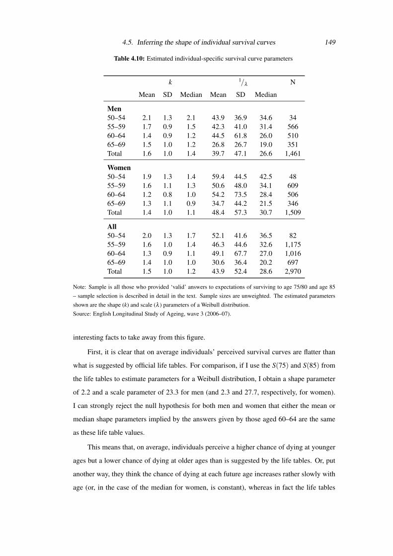
4.5. Inferring the shape of individual survival curves 149
Table 4.10: Estimated individual-specific survival curve parameters
k 1/λ N
Mean SD Median Mean SD Median
Men50–54 2.1 1.3 2.1 43.9 36.9 34.6 3455–59 1.7 0.9 1.5 42.3 41.0 31.4 56660–64 1.4 0.9 1.2 44.5 61.8 26.0 51065–69 1.5 1.0 1.2 26.8 26.7 19.0 351Total 1.6 1.0 1.4 39.7 47.1 26.6 1,461
Women50–54 1.9 1.3 1.4 59.4 44.5 42.5 4855–59 1.6 1.1 1.3 50.6 48.0 34.1 60960–64 1.2 0.8 1.0 54.2 73.5 28.4 50665–69 1.3 1.1 0.9 34.7 44.2 21.5 346Total 1.4 1.0 1.1 48.4 57.3 30.7 1,509
All50–54 2.0 1.3 1.7 52.1 41.6 36.5 8255–59 1.6 1.0 1.4 46.3 44.6 32.6 1,17560–64 1.3 0.9 1.1 49.1 67.7 27.0 1,01665–69 1.4 1.0 1.0 30.6 36.4 20.2 697Total 1.5 1.0 1.2 43.9 52.4 28.6 2,970
Note: Sample is all those who provided ‘valid’ answers to expectations of surviving to age 75/80 and age 85
– sample selection is described in detail in the text. Sample sizes are unweighted. The estimated parameters
shown are the shape (k) and scale (λ ) parameters of a Weibull distribution.
Source: English Longitudinal Study of Ageing, wave 3 (2006–07).
interesting facts to take away from this figure.
First, it is clear that on average individuals’ perceived survival curves are flatter than
what is suggested by official life tables. For comparison, if I use the S(75) and S(85) from
the life tables to estimate parameters for a Weibull distribution, I obtain a shape parameter
of 2.2 and a scale parameter of 23.3 for men (and 2.3 and 27.7, respectively, for women).
I can strongly reject the null hypothesis for both men and women that either the mean or
median shape parameters implied by the answers given by those aged 60–64 are the same
as these life table values.
This means that, on average, individuals perceive a higher chance of dying at younger
ages but a lower chance of dying at older ages than is suggested by the life tables. Or, put
another way, they think the chance of dying at each future age increases rather slowly with
age (or, in the case of the median for women, is constant), whereas in fact the life tables

150 Chapter 4. Misperceived chances of survival
Figure 4.8: Comparison of 2006 official life tables and median self-reported survival curves
Notes: Life table values are take from 2006 period life tables, for someone aged 62, produced by the Office for
National Statistics. The self-reported survival curves shown are Weibull distributions using the median shape
and scale parameters estimated from the sample of respondents aged 60–64 in ELSA wave 3 (2006–07), as
shown in Table 4.10.
suggest that mortality hazards increase much more rapidly with age. Among men, the cross-
over point – that is, the point at which individuals’ perceived probability of being dead falls
below the probability suggested by the life tables – happens at around age 82, while among
women it happens at around age 88.
The second point to note is that men’s and women’s perceived survival curves are more
similar to one another than are the life tables for men and women. Finally, among men,
although the shape of the official life table and self-perceived survival curves are different,
the average age at death is almost identical for each – at around 82 years old. (For women
the average age at death is about 3 years older according to the life tables than suggested by
the self-perceived survival curve shown in Figure 4.8.)
4.6 Implications for behaviour: two simple models
The differences between individuals’ perceived survival curves and what is suggested by life
tables have interesting and potentially important implications for life-cycle behaviour. This
section examines these. I start by presenting results from two very simple life-cycle models
4.6. Implications for behaviour: two simple models 151
of consumption and saving behaviour to highlight how different assumptions about expected
survival probabilities would affect behaviour. Based on the results of these models, I then
discuss the implications of altering assumptions about survival probabilities for life-cycle
behaviour.
4.6.1 Model 1: consumption and saving through working life and retirement
The first simple model looks at consumption and saving during working life and into retire-
ment for individuals who face uncertain income while working and an uncertain length of
life. Each individual aims to maximise his expected discounted lifetime utility, subject to
an asset accumulation process. Utility of consumption is assumed to have a constant relat-
ive risk aversion form, as shown in Equation 4.7, and individuals are assumed not to value
bequests. The coefficient of relative risk aversion (γ) is set equal to 3 (as used by Hubbard
et al., 1995; Engen et al., 1999; Scholz et al., 2006).
u(ct) =c1−γ
1− γ(4.7)
The model has 104 periods (years). t = 1 corresponds to age 25 and t = 104 ≡ T
corresponds to age 128. This upper age limit is chosen since this is the point at which
the probability of survival implied by the ‘self-perceived’ survival curve (described below)
falls below 1%. The probability of surviving from period t to period s is given by πt,s and
individuals are assumed to die with certainty by period T . Individuals are also assumed to
discount the future by a discount factor β = 0.99.
The asset accumulation process is shown in Equation 4.8, where R is a known, time-
constant rate of return on assets (2%). I also impose a no-borrowing constraint.
at+1 = R(at + yt − ct) (4.8)
Individuals face an AR(1) income process during working life, which is shown in
Equation 4.9. Where et ∼ N(0,σ2e ). Following French (2005), I set ρ = 0.977 and σ2
e =
0.0141. Individuals retire with certainty at age 65 (t = 41) and receive no more income after
this point.
lnyt = ρ lnyt−1 + et (4.9)
152 Chapter 4. Misperceived chances of survival
The resulting Bellman equation for this problem is given by Equation 4.10.
V (at ,yt) = maxat+1
(u(at ,yt ,at+1)+βπt,t+1Et
[V (at+1,yt+1)
])(4.10)
The key focus of the results from this simple life-cycle model – presented below – is to
show how simulated consumption and saving behaviour differs when different assumptions
are made about the distribution of πt,s.19 I compare the results from simulating this model
under two alternative sets of assumptions: (i) using the survival probabilities provided by
the 2006-based period life tables for men from the Office for National Statistics; (ii) us-
ing a Weibull distribution adjusted to match the properties of men’s self-reported survival
expectations described in the previous section.
Developing an appropriate distribution for (ii) is not straight-forward. The evidence
presented in the previous section relates to the shape of individuals’ perceived survival
curves from age 50 onwards. In contrast, for the model estimated here, I must specify
survival probabilities from age 25 onwards.20 I followed a three-step procedure.
First, I estimated a Weibull distribution using the S(75) and S(85) from the official
2006-based life tables (conditional on survival to age 25). This is shown, alongside the
actual life table values, in Figure 4.9. This Weibull distribution has a shape parameter (k) of
5.7 and a scale parameter(
1/λ
)equal to 59.1.
I then adjusted the shape parameter of this distribution by the ratio between the shape
parameters for the self-reported Weibull distribution shown in Figure 4.8 and the Weibull
distribution that approximates the life table survival curve also shown in Figure 4.8.21 This
adjustment gives a shape parameter of 3.1.
The third and final step was to choose a scale parameter for the self-perceived distri-
bution. The value I picked is that which ensures that the average age of death is the same
under the ‘life table’ curve and the alternative self-perceived curve. The scale parameter
that satisfies this condition is 1/λ = 62.8. The resulting alternative, self-perceived mortality
19I focus here on showing what the implications are of deviating from the standard assumption that indi-viduals have rational expectations about their chances of survival based on life table values. Of course, in themodel shown here, individuals not only face uncertainty about future survival but also about future income. AsDominitz and Manski (1997) discuss, individuals’ expectations about this may also deviate from the standardrational expectations assumption, which would also have implications for life-cycle behaviour. Considerationof this aspect of uncertainty is beyond the scope of this paper.
20To my knowledge no other survey in the UK contains questions of the sort described here for ELSA.Consequently there are no similar direct observations of the survival expectations of younger people.
21The parameters of this Weibull curve were also estimated using the S(75) and S(85) implied by the officiallife tables for a man aged 62 in 2006.

4.6. Implications for behaviour: two simple models 153
curve is shown by the dashed line in Figure 4.9.
Figure 4.9: Comparison of alternative mortality curves for 25 year-old men
Notes: Life table values are taken from 2006-based period life tables for men, conditional on survival to age 25,
produced by the Office for National Statistics. The self-perceived survival curve shown is a Weibull distribution
estimated in the way described in the text.
4.6.2 Model 2: consumption and saving through retirement
The second simple model looks specifically at consumption and saving during retirement –
taking as given that an individual arrives at the point of retirement with some stock of assets
(a0). In other words, this is a simple ‘cake-eating’ problem: the individual simply has to
decide how quickly to consume his assets. The individual aims to maximise his expected
discounted lifetime utility, given his beliefs about his chances of surviving to future periods.
Utility of consumption is again assumed to have the constant relative risk aversion form
shown in Equation 4.7, individuals are assumed not to value bequests, and the coefficient
of relative risk aversion (γ) is set equal to 3. Assets accrue a return of 2% each period
and individuals are again assumed to discount the future by a factor β = 0.99. The asset
accumulation process is shown in Equation 4.11.
at+1 = R(at − ct) (4.11)
The model has 64 periods (years). t = 1 corresponds to age 65 (i.e. the assumed date

154 Chapter 4. Misperceived chances of survival
of retirement) and t = 64 ≡ T corresponds to age 128. This upper age limit is chosen to
be consistent with the first model. The probability of surviving from period t to period s is
give by πt,s and individuals are assumed to die with certainty by period T . The resulting
Bellman equation for this problem is given by Equation 4.12.
V (at) = maxat+1
(u(at ,at+1)+βπt,t+1
[V (at+1)
])(4.12)
I estimate this model under two alternative sets of assumptions about future survival
akin to those described for the first model. The first assumption is that individuals face the
mortality probabilities suggested by the official 2006-based period life tables for English
men, conditional on having survived to age 65. The second assumption is that individu-
als face some flatter self-perceived mortality curve, estimated in an analogous way to that
described above for the first model. Both these survival curves are shown in Figure 4.10.
Figure 4.10: Comparison of alternative mortality curves for 65 year-old men
Notes: As Figure 4.9.
4.6.3 Implications for life-cycle behaviour
The key results from these two models are presented in Figures 4.11 and 4.12. Each of these
highlights interesting predictions for life-cycle behaviour if we deviate from the standard
assumption that individuals hold rational expectations about population-average survival
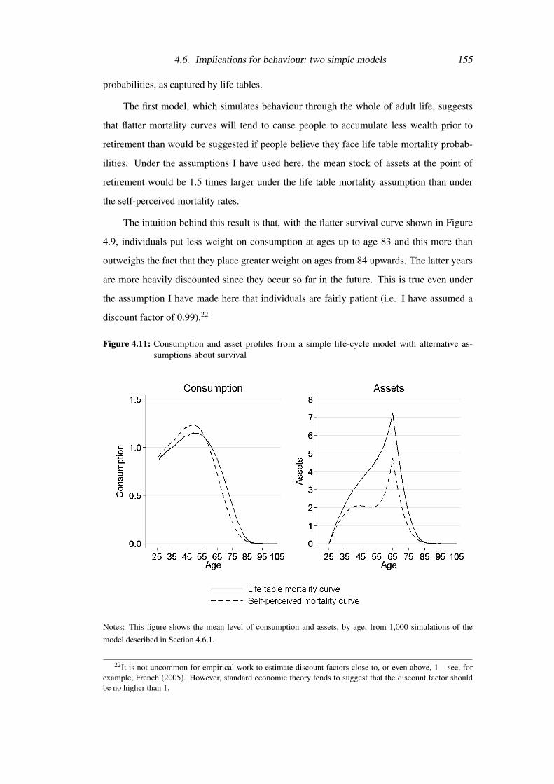
4.6. Implications for behaviour: two simple models 155
probabilities, as captured by life tables.
The first model, which simulates behaviour through the whole of adult life, suggests
that flatter mortality curves will tend to cause people to accumulate less wealth prior to
retirement than would be suggested if people believe they face life table mortality probab-
ilities. Under the assumptions I have used here, the mean stock of assets at the point of
retirement would be 1.5 times larger under the life table mortality assumption than under
the self-perceived mortality rates.
The intuition behind this result is that, with the flatter survival curve shown in Figure
4.9, individuals put less weight on consumption at ages up to age 83 and this more than
outweighs the fact that they place greater weight on ages from 84 upwards. The latter years
are more heavily discounted since they occur so far in the future. This is true even under
the assumption I have made here that individuals are fairly patient (i.e. I have assumed a
discount factor of 0.99).22
Figure 4.11: Consumption and asset profiles from a simple life-cycle model with alternative as-sumptions about survival
Notes: This figure shows the mean level of consumption and assets, by age, from 1,000 simulations of the
model described in Section 4.6.1.
22It is not uncommon for empirical work to estimate discount factors close to, or even above, 1 – see, forexample, French (2005). However, standard economic theory tends to suggest that the discount factor shouldbe no higher than 1.

156 Chapter 4. Misperceived chances of survival
The second model focuses on asset decumulation during retirement. The results shown
in Figure 4.12 demonstrate that a flatter survival curve leads to individuals consuming more
in the early years of retirement but then decumulating assets less rapidly after age 80. For
example, as the left-hand panel of Figure 4.12 shows, desired consumption in the first year
of retirement would be 20% higher under the flatter survival curve than if the individual
believed he faced the life table mortality probabilities.
Figure 4.12: Consumption and asset profiles from a simple cake-eating model with alternative as-sumptions about survival
Notes: This figure shows the level of consumption and assets, by age, from 1,000 simulations of the model
described in Section 4.6.2.
These insights have potentially important implications for understanding individual
behaviour. The models’ results also hint at a potential explanation for some puzzles that
have been widely debated in the economic literature.
First, Figure 4.11 suggests that individuals will tend to save less for their retirement
than they otherwise would because they over-estimate their chance of dying young. This
could provide a rationale for governments intervening to encourage or force people to save
more in pensions during their working lives. This has been the direction of travel for UK
public policy over recent years, with the introduction of automatic enrolment into workplace
pension schemes. Alternatively, the government could try to address the same issue by

4.6. Implications for behaviour: two simple models 157
helping to ensure people are better informed about their chances of survival.
Second, Figure 4.11 also suggests that consumption would drop more sharply after
retirement under the self-perceived survival curves than under the life table curves. This
could provide a partial explanation for the much-debated retirement-savings puzzle (Banks,
Blundell, and Tanner, 1998).
Third, the insights from the second model could also help explain why demand for
annuities is lower than standard economic models suggest (Fang, 2014) and why (in the UK
at least) the vast majority of people purchasing annuities have opted to purchase nominal
annuities – that is, annuities that pay out higher real income upfront and lower real income
later on – even though price-indexed annuities are readily available.
In determining the price for an annuity, insurance companies will incorporate their best
estimate of the chance that the purchaser will survive to future years. If their assessment
of the mortality curve is steeper than individuals’ own perceptions, then the price offered
may prove unattractive to the individual, even though it may be a fair offer (on the basis
of the information available to the insurer). For example, a recent paper by Lowe (2014)
concluded that many annuity rates offered in the UK provided fair value for money, but that
there was still a widespread public perception that this was not the case.
Fourth, the insights from the second model could help explain why people decumulate
wealth more slowly towards the end of life than many life-cycle models suggest. This is
an alternative explanation to that suggested by De Nardi, French, and Jones (2010), who
highlight the importance of the risk of large medical expenses towards the end of life in ex-
plaining slow wealth decumulation among older American households. It is also potentially
consistent with the related finding from Blundell et al. (2016) that wealth decumulation is, if
anything, even slower among older English households than among American households –
despite the fact that (arguably) the former face lower risk of high end-of-life medical costs.
Fifth, flatter survival curves would also imply that individuals should value highly
insurance against the costs of late-life medical expenses and long-term care. This is not
captured by the very simple models presented here. However, since these are costs that
typically occur after age 80,23 the flatter self-perceived survival curves shown in Figures
4.9 and 4.10 would imply that individuals should place more weight on costs occurring at
those older ages than would be the case if they acted according to life table values. In other
23Figure 9 of Blundell et al. (2016) shows that this is the case for older American households.

158 Chapter 4. Misperceived chances of survival
words, this is a market where we would expect to find the reverse of what is seen in the
annuity market. That is, individuals will tend to value this insurance quite highly – since
they expect a relatively high chance of surviving to old age – while insurers will tend to
expect purchasers to die more quickly.24
The results presented above were estimated using survival curves that approximate
those reported on average by men in the ELSA data. However, as highlighted in the previous
section, if anything women appear to underestimate their chances of surviving to younger
ages more severely than men (and overestimate their chances of surviving to very old age
less severely). Indeed men and women appear to hold beliefs about their chances of survival
that are more similar to one another than life tables suggest. This means that, if anything,
the first three behaviours described above would be more exaggerated for women than for
men. This suggests that there might be a particular concern about women under-saving for
retirement and under-valuing annuities when they reach retirement.
4.7 Conclusions
Individuals’ expectations of the probability that they will survive to future periods play an
important role in life-cycle models of behaviour, when individuals are assumed to make
decisions in the presence of partial information about future events, including their own
survival. Optimal decisions about how much to work, consume and save in any period will
depend importantly on how likely someone thinks it is that she will be alive in the future. It
is well established that, in practice, survival rates are very different across different groups
– for example, certain health conditions and behaviours are known to affect chances of
survival directly, while a number of other socioeconomic characteristics are also known to
be related to (though possibly not causal of) shorter life expectancy.
Despite the importance of this, most papers that estimate life-cycle models of beha-
viour do so assuming that individuals face population average, sex-specific life tables and
that they have rational expectations about this. Such models typically infer individual pref-
erences from observed behaviour, assuming individuals aim to maximise expected utility
with expectations of survival given by population life tables.
However, in practice, observed behaviour may be consistent with a number of differ-
ent sets of expectations and preferences. Therefore, if in fact expectations are not well-
24This line of argument relies on individuals having good information about the risk of nursing home costsand the age at which these are likely to be incurred. In practice individuals may not be well-informed aboutthis.

4.7. Conclusions 159
approximated by the life table values, the inferred preference parameters will be incorrect.
In recognition of the importance of individuals’ own survival expectations in explaining
their behaviour, a number of surveys have now attempted to elicit information on these –
Manski (2004) provides a useful summary of the literature. In particular, a number of sur-
veys now seek to elicit individuals’ probabilistic expectations of future events, including
their own survival to certain older ages, which can be used to relax the standard assump-
tions.
This paper has shown that individuals’ expectations of survival do not match the shape
of official life tables. In particular, people appear to underestimate the chances of surviving
to younger ages but overestimate the chances of surviving to very old age. Incorporating
such survival expectations into a life-cycle model would have important implications for
the interpretation and prediction of behaviour. Flatter survival curves imply that individuals
face greater uncertainty about the age at which they will die. Depending on an individual’s
degree of risk aversion, this will affect how they will behave.
Using two simple life cycle models of consumption and saving I show that these flatter
survival curves could help explain a number of apparently puzzling aspects of individual
behaviour. This includes under-saving for retirement, sharp drops in consumption at retire-
ment, low demand for annuities and slow wealth decumulation in old age.
The results from these simple models suggest that there could be significant value in
attempting to build heterogeneity in survival expectations and systematic deviations from
life table values into more complex dynamic life cycle models to help better understand
individuals’ behaviour. This driver of individuals’ behaviour deserves some of the same
attention that has been devoted to understanding heterogeneity in discount rates.
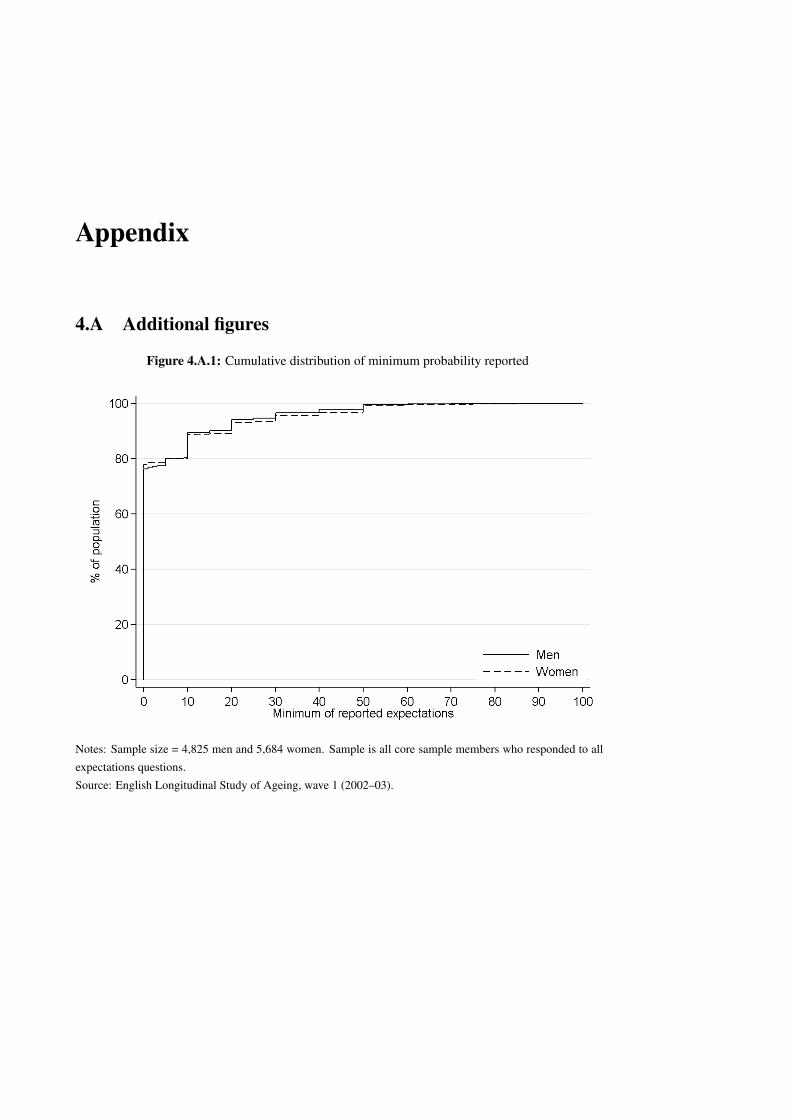
Appendix
4.A Additional figures
Figure 4.A.1: Cumulative distribution of minimum probability reported
Notes: Sample size = 4,825 men and 5,684 women. Sample is all core sample members who responded to all
expectations questions.
Source: English Longitudinal Study of Ageing, wave 1 (2002–03).

4.A. Additional figures 161
Figure 4.A.2: Cumulative distribution of maximum probability reported
Notes and sources: As Figure 4.A.1.
Figure 4.A.3: Cumulative distribution of range of probabilities reported
Notes and sources: As Figure 4.A.1.


Chapter 5
Private information and adverse selection in
the market for annuities
5.1 Introduction1
Private information can affect the existence, nature and efficiency of market equilibria. In
some circumstances this can justify a role for government intervention to improve effi-
ciency. However, what intervention is appropriate will depend on the nature and extent of
the private information. In this paper, I test for the existence of informational asymmetries
– in particular about risk type – in the annuity market in the United Kingdom (UK). I am
able to shed interesting new light on this question by making use of detailed household
survey data which allows me to observe not only the characteristics of individuals that are
used in pricing annuities but also individuals’ own expectations of the insured risk, other
characteristics, behaviours, preferences and experience of the relevant risk (i.e. survival to
older ages).
This is a market in which it is easy to believe that there could be a problem of private
information. Most annuity policies are priced only on the basis of age, sex and location
of residence, while purchasers may well know much more about (for example) their state
of health, whether they engage in good health behaviours and whether they take prevent-
ative health measures. Indeed, as Chapter 4 showed, individuals’ expectations of their
own longevity are predictive of subsequent survival over and above age, sex and numer-
ous doctor-diagnosed health conditions.
The analysis presented here is only possible with the unique combination of data and
1I am very grateful to James Banks and Agar Brugiavini for detailed discussions about this work. Thischapter has also benefited from comments received from seminar participants at University College Londonand the Superintendencia de Pensiones, Santiago.
164 Chapter 5. Private information and adverse selection
institutional framework that exists in England. The specific pensions policies in the UK
mean that a much larger fraction of the older population buy annuities than in most other
countries. As a result, it is possible to use household microdata to compare annuitants and
non-annuitants. These detailed microdata contain considerably richer information than is
typically available from insurance companies’ administrative data, which has been used in
previous work on this subject (for example, Finkelstein and Poterba, 2002, 2004, 2014).
Many empirical studies of adverse selection in the annuity market (and in other in-
surance markets) have been based on the theoretical observation that, if adverse selection
exists, among observationally equivalent individuals2 those who purchase insurance should
be found to have a higher (ex post) incidence of the (potentially) insured risk than those
who do not have insurance. As Chiappori and Salanie (2000) argue, this relationship should
hold under quite general conditions.
Using tests of this type, a number of papers have found evidence of adverse selection
in the market for annuities and, in particular, the UK annuity market. Using data from indi-
vidual insurance companies in the UK, Finkelstein and Poterba (2002, 2004) find evidence
that is consistent with standard models of adverse selection. Using data on mortality of
annuitants and non-annuitants in the United States (US) Friedman and Warshawsky (1990)
find that annuitants live longer than non-annuitants; a similar result is found by McCarthy
and Mitchell (2003) for annuitants in the US and UK. Using data on life annuities sold
by the UK government in the nineteenth century, Rothschild (2009) also finds evidence of
significant adverse selection.
However, this type of test suffers from two potential drawbacks.3 First, the positive
correlation test could be invalid if there are multiple dimensions of private information. As
de Meza and Webb (2001) point out, if there are multiple dimensions of private inform-
ation, the positive correlation test may be spuriously passed/failed even if there is not/is
2More specifically, one should focus on comparing the riskiness of individuals with and without insurancewho would be offered the same contract by an insurance company – that is, they are identical to one another interms of all characteristics that insurers use in pricing insurance policies.
3A third drawback of these positive correlation tests in most insurance markets is that they cannot dis-tinguish between adverse selection and moral hazard. Moral hazard would also lead to this same positiverelationship between the amount of insurance purchased and the probability of experiencing a loss (Arnott andStiglitz, 1988): the larger the quantity of insurance an individual buys, the less incentive they have to try tomitigate their exposure to risk. However, it seems unlikely that moral hazard will be a serious concern in themarket for annuities. In this market moral hazard would require that people take additional care to keep them-selves alive simply in order to be able to receive larger sums from their annuities. It seems unlikely that thiswould be a serious concern. (This is notwithstanding Mrs Dashwood’s observation in Sense and Sensibility that‘people always live forever when there is an annuity to be paid them’ (Austen, 1811, chapter 2).)

5.1. Introduction 165
adverse selection. In particular, if individuals differ in their degree of (privately known) risk
aversion and this is negatively correlated with their riskiness, lower risk individuals will
tend to demand more insurance (Jullien, Salanie, and Salanie, 2007). This phenomenon
has been termed ‘advantageous’ or ‘propitious’ selection.4 In most insurance markets this
advantageous selection will tend to counteract any adverse selection, thus diminishing (or
even reversing) the expected positive correlation between insurance coverage and riskiness
(Chiappori et al., 2006). However, in the market for annuities these effects are likely to act
in the same direction.
Second, it is not clear from standard positive correlation tests whether adverse selection
is ‘active’ or ‘passive’ (Finkelstein and Poterba, 2002). That is, whether individuals who
buy annuities are aware that they are likely to live a relatively long time or whether they
simply have other characteristics (such as higher wealth) that are correlated with survival
but (for whatever reason) are not used by insurers in pricing annuities.
In this paper I use household survey data from England to test for evidence of inform-
ational asymmetries – and in particular adverse selection – in the market for annuities. I
provide some important contributions to the existing literature. First, I show that there is
still a positive correlation between annuity purchase and survival even taking into account
detailed measures of residential location and current health and health behaviours. Previous
work by Finkelstein and Poterba (2002, 2004, 2014) used data from a period when insurers
used (surprisingly) little information in distinguishing prices of annuities. More recently,
pricing formulae have become significantly more sophisticated in the UK. Second, by look-
ing directly at the relationship between survival expectations and annuity purchases, I show
that this selection into annuity purchase is active – that is, annuity holders expect to live
longer than their (observationally equivalent) counterparts who do not purchase annuities. I
also use complementary survey data to shed some light on the source of the private informa-
tion that individuals appear to have about their chances of survival. Finally, for a subsample
of individuals I am also able to look at financial risk preferences, which provides tentative
evidence on the potential additional importance of differences in risk preferences in driving
the observed patterns of annuity holding.
I choose to focus on annuity markets for a number of reasons. First, the insured risk
in annuity markets (survival) is easily observed and so I can obtain a good measure of indi-
4The first paper to describe this phenomenon was Hemenway (1990).

166 Chapter 5. Private information and adverse selection
viduals’ experience of this (binary) risk (and thus their actual claims on their ‘insurance’),
which is often not the case in other insurance markets. Second, as discussed above, private
information about preference heterogeneity has different implications in annuity markets
than it does in other insurance markets. Third, and most importantly, studying annuity mar-
kets is of significant interest in its own right. In 2013 there were over 350,000 annuities
sold in the UK, worth a total of £11.9 billion or 0.7% of GDP (Association of British In-
surers, 2014). Furthermore, given the growing debates worldwide about how to avoid public
pension expenditure becoming unsustainable and how encouraging private saving can help
this, annuity products are likely to play an increasingly important role in helping individuals
achieve their desired standard of living through retirement in many countries.
Having said this, while many countries are shifting towards a greater role for annuities
in providing retirement income, the UK has actually recently implemented reforms that
move in the opposite direction. At the end of this paper I discuss the importance of my
findings in the context of these reforms.
Section 5.2 starts by reviewing the existing related literature. Section 5.3 then describes
the important features of the annuity market in the UK. Section 5.4 describes the data that I
use and presents descriptive statistics on the sample. Section 5.5 describes the econometric
methodology for testing for adverse selection and other forms of informational asymmetry
in detail, with results presented in Section 5.6. Section 5.7 presents evidence on the rela-
tionship between riskiness and risk preferences. Section 5.8 discusses the implications of
the results and concludes.
5.2 Related literature
5.2.1 Adverse selection in annuity markets
Following the seminal work of Akerlof (1970), a large literature has grown up examining
informational asymmetries between economic agents and situations in which these affect
the existence and efficiency of the competitive equilibrium. One example of this is private
information in insurance markets: that is, the possibility that purchasers of insurance have
more information about their own risk type (and, therefore, the expected pay-off to any
contract signed) than insurers do.
The potential for adverse selection to exist has been clearly demonstrated in theory
(Rothschild and Stiglitz, 1976) and is often used by economists to justify government inter-
vention in these markets. However, empirical evidence on the existence of adverse selection

5.2. Related literature 167
in insurance markets has been rather mixed – with studies finding evidence of it in some in-
surance markets and/or within some risk pools but absent elsewhere (Cohen and Siegelman,
2010).
Using the positive correlation test suggested by Chiappori and Salanie (2000), a num-
ber of papers have found results that are inconsistent with the presence of adverse selection
in a number of different insurance markets. These include Cawley and Philipson (1999) and
Hendel and Lizzeri (2003) on the US life insurance market, Chiappori and Salanie (2000)
on the French automobile insurance market and Cardon and Hendel (2001) on the US health
insurance market. However, other studies have concluded that asymmetries in information
are important in some settings. For example, He (2009) finds evidence of adverse selection
in the US life insurance market when she focuses on the population of potential purchasers.
The market for annuities is the exception in the sense that positive correlation tests
have consistently pointed towards the presence of adverse selection (Finkelstein and Po-
terba, 2002, 2004; McCarthy and Mitchell, 2003; Rothschild, 2009). Finkelstein and Po-
terba (2014) confirm this finding and demonstrate that it is not merely driven by differences
in preferences between annuitants and non-annuitants by using an ‘unused observables’
test. The unused observables test they propose relies on finding some characteristic that
is known to be correlated with survival but which is not used in pricing annuities. Using
data on annuities sold by a particular insurance company in the late 1980s and 1990s, they
show that residential location was just such an unused observable and that it is significantly
correlated with annuity demand – thus indicating the presence of adverse selection. Wup-
perman (2010) also shows that one reason for the greater adverse selection found in annuity
markets compared to life insurance markets may be the more limited underwriting criteria
used in the former market than the latter.
One question raised by Finkelstein and Poterba (2014)’s analysis is why insurers did
not use residential location information when pricing annuities, given that it was easily
observed. (Indeed the reason Finkelstein and Poterba were able to conduct their test at all
was because they had data from the insurer on purchasers’ addresses even though it had not
been used in setting the price.) Over the last decade (after the period that Finkelstein and
Poterba studied in their papers) annuity pricing in the UK has become more sophisticated.
It is now common for annuity providers to offer different prices to people living in different
areas and there are also a number of providers who specialise in offering ‘impaired’ and

168 Chapter 5. Private information and adverse selection
‘enhanced’ life annuities to those who can show they are in poor health or engage in life-
limiting behaviours (such as smoking). In this paper I demonstrate that even these more
sophisticated underwriting criteria are unlikely to have completely mitigated the adverse
selection in this market.
While Finkelstein and Poterba (2014) show that adverse selection does exist, they can-
not establish whether it is ‘active’ or ‘passive’. As Finkelstein and Poterba (2002) discuss,
active adverse selection would occur when individuals know their risk type, whereas passive
selection would occur if annuity purchases are correlated with some other factor that is also
related to the probability of surviving, even if the individuals are unaware of this. Both of
these types of adverse selection could lead to welfare losses but the appropriate response to
each may be different. Here I look directly at the relationship between annuity purchase and
individuals’ actual knowledge of the insured risk (i.e. survival to old age); to my knowledge
no other paper has done this.
It has also been hypothesised that multiple dimensions of private information may be
at work in insurance markets. One particular form of private information that has been
discussed is differences in risk preferences among more and less risky types (Hemenway,
1990). If individuals differ in their degree of (privately known) risk aversion and this is
negatively correlated with riskiness, lower risk individuals will tend to demand more insur-
ance (de Meza and Webb, 2001; Jullien, Salanie, and Salanie, 2007) – this has been termed
‘advantageous’ or ‘propitious’ selection.
In most markets, this advantageous selection will counteract any adverse selection. For
example, using evidence on long-term care insurance in the US, Finkelstein and McGarry
(2006) find that – even though individuals’ own assessments of their riskiness are positively
correlated with both their probability of experiencing a loss and their insurance coverage –
there is no evidence of a direct positive correlation between the amount of insurance that
an individual has and their chance of experiencing a loss. They conclude that this failure
of the positive correlation test is indicative of the existence of advantageous selection in the
market as well: that is, there is a negative correlation between individuals’ actual riskiness
and their risk aversion. This negative correlation offsets the expected positive correlation
arising from adverse selection.
While advantageous selection will offset adverse selection in most insurance markets,
the reverse is true in the annuity market. It has, therefore, been suggested that this could

5.3. Institutional background 169
explain the apparently contradictory empirical evidence that there is adverse selection in
annuity markets but not in the market for life insurance – two products that, in theory, insure
opposite sides of the same risk (Finkelstein and McGarry, 2006; Finkelstein and Poterba,
2014).
5.2.2 Private information about health
To the extent that I examine the size and nature of individuals’ private information about
their health, this paper also contributes to a related but separate literature that has looked
directly at private information about health. Idler and Benyamini (1997) provide a use-
ful review of many older papers. More recent work, which has also attempted to examine
whether the degree of private information about health changes with age, include Burstrom
and Fredlund (2001), van Doorslaer and Gerdtham (2003) and Banks, Crossley, and Gos-
hev (2007). Papers in this literature have mainly focussed on exploring to what extent
self-assessed health is predictive of future health and mortality over-and-above diagnosed
conditions.
The existence of ‘private’ information about health (whether in the sense of being
unknown to other market players, to researchers or to both) has potentially important im-
plications beyond insurance markets, since expectations of future health may affect (among
other things) individuals’ decisions about precautionary saving, investment in human cap-
ital and wealth decumulation. However, my discussion in the rest of this paper focusses on
the existence and importance of private information about health specifically in the annuity
market.
5.3 Institutional background5
Pension saving in the UK attracts EET tax treatment – that is, contributions are made from
pre-tax income, interest earned on pension investments is also tax-free, but pension in-
come is taxed on receipt.6 Until April 2015, the UK government required individuals who
had accumulated funds in tax-favoured defined contribution (DC) pension savings vehicles
(similar to IRAs or 401(k)s in the US) to purchase an annuity with at least 75% of the fund
before the age of 75. As a result, the UK annuity market is better developed and ‘thicker’
than most other developed countries’ annuity markets. Therefore, while the functioning of
5The description in this section relates to policies in place prior to April 2011, as the data I use was collectedbefore that date. Some major policy changes have been announced and enacted since then. These are discussedin Section 5.8.
6The one exception is that up to 25% of pension funds can be withdrawn tax free.
170 Chapter 5. Private information and adverse selection
annuity markets is of concern to a large number of countries, it is the UK annuity market
that has received a lot of attention in the economic literature.
At first glance, it may seem odd to look for adverse selection in a market where pur-
chase of insurance is ‘compulsory’. However, there are two opportunities for ‘selection’ in
the sample I examine which could cause annuitants to be found to have higher survival rates
than observationally-equivalent non-annuitants.
First, for the cohorts I examine, there may have been a degree of selection into DC
pension saving in the first place. The DC pension market only expanded significantly from
the late 1980s onwards.7 Therefore, among the sample I examine (those born between 1933
and 1956), many will have been relatively old when they first opted to put money into a DC
pension. In other words, their choice to save in a DC pension at all may reflect knowledge
about their own expected longevity.
Second, annuitisation was only compulsory at the age of 75. Prior to that age, indi-
viduals could choose to leave their funds in their DC pension and thus retain the option of
bequeathing the funds to their heirs when they died. Therefore, in the empirical analysis, I
focus just on those aged under 70, thereby contrasting those who chose to annuitise earlier
than they were required to with those who avoided doing so.
In addition to this ‘compulsory’ annuity market in the UK there is also a separate ‘vol-
untary’ annuity market. That is, there are a separate set of annuity products that individuals
can choose to buy using a cash lump sum, which has not been taken out of a DC pension.
This is an entirely separate market. The prices charged in this market are different from
those charged to people buying an annuity using DC pension funds (Cannon and Tonks,
2006). Income from these annuities is also taxed differently from income from DC pen-
sion annuities – because voluntary annuities are purchased using funds saved from taxed
income, income from voluntary annuities is taxed at a much lower rate than income from
DC pension annuities.
In principle, we might expect more severe adverse in the voluntary annuity market than
the compulsory market (as Finkelstein and Poterba, 2002, found) and comparing behaviour
and experience between purchasers in the two markets should provide an additional test
of private information. However, purchases of voluntary annuities are uncommon and so
7From 1987 onwards it became possible to opt out of the state second tier pension, in return for a reductionin social insurance contributions, and instead make contributions to a DC pension scheme. As a result, DCpension saving expanded significantly after 1987 but had been very limited before then.

5.4. Data 171
the survey data I use does not provide sufficient power to distinguish differences between
these two groups. Therefore I examine both types of annuitants and compare them to non-
annuitants.
5.4 Data
I use data from the first five waves of the English Longitudinal Study of Ageing (ELSA),
collected between 2002–03 and 2010–11. These data provide four key pieces of informa-
tion that are crucial to the analysis. First, I observe whether or not respondents hold any
form of annuity. Second, I observe detailed information on individuals’ circumstances that
allow me to proxy insurers’ risk categorisations. Third, I have very accurate information on
whether or not respondents die and, if so, when. Fourth, I observe individuals’ self-reported
expectations of surviving to older ages, allowing me to examine what (potentially private)
information individuals have about their future longevity. The rest of this section describes
each of these elements in some more detail and presents descriptive statistics on the sample
used.
ELSA is a survey of a representative sample of the household population in England
aged 50 and over. Respondents have been interviewed every two years since 2002–03, with
refreshment samples added in the third and fourth waves to account for attrition and also to
add in later cohorts to retain representation of the age 50+ population.
Information on mortality is gathered from official death records (from the National
Health Service Central Register, NHSCR) and/or from respondents’ surviving family or
friends. 95% of ELSA respondents gave permission for their outcomes to be tracked through
the NHSCR even if they attrit from the survey. I therefore have virtually complete informa-
tion on the subsequent mortality of all respondents. This information is currently available
up to February 2013 – that is, providing a minimum of two years’ mortality follow-up for
each survey respondent since their interviews in waves 1–5.8
The ELSA questionnaire is modelled on the US Health and Retirement Study and con-
tains detailed questions on a range of areas, including the economic, social and demographic
circumstances, health, cognitive functioning and expectations of the older population. In
addition, respondents were visited by a nurse after their interviews in waves 2 and 4.
In this paper, I focus on the sample of individuals aged between 55 and 69. Age 55
8Data from the sixth wave of ELSA (2012–13) are also available. However, I do not use them in this paperas I only have information on deaths up to February 2013. Therefore I do not discuss the sixth wave of datahere.

172 Chapter 5. Private information and adverse selection
is chosen as the bottom of the age range because, since April 2010, individuals have not
been able to access their tax-favoured pension savings until age 55. The age of 69 is chosen
as the upper age cut-off to avoid including those people who may have been compelled to
annuitise by their proximity to age 75.
In total there were 25,198 observations (on 9,821 distinct core sample members aged
between 55 and 69) in waves 1–5. However, for 3,689 of these observations (on 1,725 indi-
viduals) at least one of the required question responses was missing. The most commonly
missing piece of information was father’s age at death, followed by mother’s age at death.
In addition, there are two pieces of information that are not available in every wave of
the survey: these are body mass index (BMI) and quintile of the index of multiple depriva-
tion.9 For waves where these are missing, I have used responses to earlier or later waves as a
proxy. However, since some individuals did not respond in other waves, this further reduces
the available sample size to a total of 17,290 observations on 5,565 unique individuals.
5.4.1 Identifying annuity holders in the ELSA data
Compulsory annuities are those purchased from funds accumulated in tax-favoured DC
pensions, while voluntary annuities are those purchased using any other funds. Identifying
holders of voluntary annuities in the ELSA data is straightforward. However, the questions
asked in the first two waves of ELSA do not allow me to identify compulsory annuities
perfectly. By making use of information collected in subsequent waves, I am able to fill
in this information for most of my sample. For those for whom the information is still
missing – that is, some individuals who are known to be receiving an income from a pension
product, but where I do not know whether or not any part of this comes from a compulsory
annuity or whether it is all being provided by defined benefit (DB) pension schemes – I
classify these individuals as not having an annuity. This assumption will tend to bias my
results to finding smaller differences between annuitants and non-annuitants, as I may have
misclassified these individuals.
5.4.2 Self-reported expectations of survival
Respondents to ELSA are asked a series of questions about what chance they think there is
of certain future events happening. This includes their expectation that they will live to some
specific future age. Those aged under 66 were asked about survival to age 75; those aged
9The latter is in principle available for all waves but a special licence is required to use these data. I am stillawaiting permission to use the more detailed geographic data for some of the waves of ELSA.

5.4. Data 173
66–69 were asked about survival to age 80. This means that all the respondents included in
my sample were asked about their chances of surviving for somewhere between 10 and 20
years.
The way that these questions were asked and the patterns of response are described
in considerably more detail in Chapter 4. The analysis presented there suggests that, on
average, self-reported expectations of survival appear sensible. Expectations are correlated
with known risk factors and with subsequent outcomes. It also appears that survival ex-
pectations include an ‘expectational’ component that is not fully explained by measures of
current health. This suggests that there is scope for adverse selection to be a problem in the
annuity market.
5.4.3 Measuring health
ELSA contains a wide range of indicators of individuals’ health. In this paper, I focus on
those measures that are used in underwriting some types of annuity policies. Most annuity
policies do not explicitly factor purchasers’ health into the price. However, over the last
decade an increasingly sophisticated market providing ‘enhanced’ or ‘impaired’ life annuit-
ies has developed. This market (which accounted for 2% of annuities sold in 2003, rising to
24% in 2012, (Association of British Insurers, 2014)) offers lower-priced annuities specific-
ally to individuals whose life expectancy is likely to be limited, either because they engage
in unhealthy behaviours (enhanced life annuities) or because they have been diagnosed with
some life-limiting condition (impaired life annuities). Appendix 5.B provides a full list of
conditions that would typically qualify someone for an enhanced or impaired life annuity.
Diagnoses of most of these conditions are reported in ELSA and can be controlled for in
the analysis.
Enhanced life annuities are available to those who smoke or who are overweight. I
use indicators of self-reported smoking behaviour and nurse measurements of BMI to cap-
ture these factors. Measures of BMI are only available from the ELSA nurse visits, which
were conducted in waves 2, 4 and 6. For waves where this information is missing, I proxy
contemporaneous BMI using the measurement taken in the closest available nurse visit. A
more extensive description of the nurse visits and how height and weight were measured is
provided in Appendix 5.C.
Impaired life annuities are available to those who have been diagnosed with one of a
range of serious health conditions. Virtually all of the relevant conditions are asked about

174 Chapter 5. Private information and adverse selection
in the ELSA survey. I can therefore control for them using self-reported doctor diagnoses.
5.4.4 Measuring risk preferences
In the fifth wave of ELSA (2010–11) an experimental module was fielded, which aimed to
assess respondents’ time and (financial) risk preferences. This was done using a series of
choice tasks (or games).10 Attached to these tasks were small but real pay-offs. In total
1,063 respondents aged between 50 and 75 took part in this module.
Financial risk tolerance was measured experimentally using ten Eckel-Grossman tasks
(Eckel and Grossman, 2002, 2008). In these tasks, respondents are given a choice between
six lotteries, each of which gives a 50:50 chance of winning one of two different amounts
of ‘money’.11 The options given range from complete certainty to lotteries with greater
variance in the potential pay-off.
In this paper, I focus on choices made in the ‘baseline’ task, which was adopted from
Dave et al. (2010). This gave respondents the choice between the following six lotteries
(with a 50:50 chance of each outcome in each lottery): 28/28, 24/26, 20/44, 16/52, 12/60,
2/70. It is worth noting that the final two options provide the same expected pay-off but the
2/70 lottery offers greater variance in the outcome than the 12/60 lottery. In other words,
choosing the final option would suggest the respondent is risk loving.
In addition to this task-based measure of risk preference, respondents were also asked
to rate their own attitude to risk. The wording of this question was not explicitly about
financial risk taking but rather about risk taking in general. Specifically, they were asked to
rate (on a scale from 0 to 10) whether ‘you are generally a person who is fully prepared to
take risk or do you try to avoid taking risks?’. Where 0 denoted ‘avoid taking risks’ and 10
denoted ‘fully prepared to take risks’.12
Of the 1,106 respondents who were randomised into the module, 43 refused to take
part. Of the 1,063 who agreed to participate, all completed the baseline risk preference task
and all but 2 reported an answer about their own perceptions of their willingness to take
risks. In this paper I focus on responses provided by the 792 respondents who were aged
10A full description of the questions asked can be found in National Centre for Social Research (2012). Apreliminary description of the results from this module can be found in Alan et al. (2012).
11At the end of the module, the computer randomly picked one of the games played by the respondent andthe respondent won the amount of money corresponding to the choices they made in that game. There weretherefore real (though small) rewards attached to the choices made. Respondents were told that this wouldhappen at the start of the module.
12This question wording was adopted from the Understanding Society survey, which is a panel study of theBritish household population, covering all age groups.

5.4. Data 175
between 55 and 69.
5.4.5 Descriptive statistics
Tables 5.1–5.3 compare the characteristics between my sample of annuitants and non-
annuitants. Table 5.1 shows that 21.5% of my sample have some sort of annuity. 11.9%
of my sample of annuitants holds a voluntary annuity, while 93.7% hold a compulsory an-
nuity – implying that 5.6% hold both types of annuities. On average annuitants are slightly
older than non-annuitants. Men are also much more likely than women to hold annuities.
Table 5.1 also describes individuals’ responses to a question about their expectations of
surviving to a future age. First, the table describes the average self-reported expectations of
surviving in each group. This shows that the average self-reported chance is not statistically
significantly different between annuitants and non-annuitants – non-annuitants on average
report a 65.1% chance of survival, while annuitants report on average a 65.2% chance. This
is consistent with the evidence in the bottom row of the table that both groups were equally
likely to survive for at least two years following interview. However, this comparison of
self-reported expectations of survival appears to hide differences in the age/sex composi-
tion of annuitants and non-annuitants. Also reported in the table is an alternative measure
of expectations – the residual from a regression of self-reported survival expectations on
dummies for each sex/year-of-age/year-of-interview combination. This measure captures
the deviation between each person’s answer and the average answer among other people of
the same age and sex interviewed in the same wave. This suggests that annuitants on aver-
age report survival expectations that are 1.0 percentage points higher than other people of
the same age and sex. If age and sex were the only characteristics used in pricing annuities,
this in itself would be evidence of adverse selection.
There are also some interesting differences in health and health behaviours between
annuitants and non-annuitants (Table 5.2). Annuitants and non-annuitants are equally as
likely as one another never to have smoked. However, annuitants are more likely than non-
annuitants to be former smokers, while non-annuitants are more likely still to be smoking.
The patterns of diagnosed health conditions are mixed. Annuitants are more likely
than non-annuitants to have been diagnosed with hypertension (high blood pressure), vari-
ous heart conditions, diabetes, cancer and Parkinson’s disease but less likely to have been
diagnosed with asthma, osteoporosis or psychiatric problems. Overall, non-annuitants are
significantly more likely to describe themselves as being in ‘fair’ or ‘poor’ health than an-

176 Chapter 5. Private information and adverse selection
Table 5.1: Demographic characteristics
% (except where otherwise stated) No annuity Has annuity Diff. p-value
Age (years) 61.4 64.0 –2.6 0.000***
Date of interview2002–03 24.3 18.3 6.0 0.000***2004–05 22.9 20.5 2.4 0.002***2006–07 22.4 19.9 2.5 0.001***2008–09 15.8 19.4 –3.6 0.000***2010–11 14.6 21.8 –7.3 0.000***
Male 43.1 54.3 –11.2 0.000***
RegionNorth East 6.7 5.2 1.4 0.001***North West 11.5 12.6 –1.1 0.068*Yorkshire and the Humber 11.6 10.7 0.9 0.119East Midlands 10.9 10.2 0.6 0.266West Midlands 10.5 10.7 –0.2 0.755East of England 12.5 14.4 –1.9 0.003***London 9.4 7.2 2.2 0.000***South East 16.3 17.1 –0.8 0.248South West 10.7 11.8 –1.1 0.056*
Area-level deprivationLeast deprived 25.5 26.3 –0.8 0.303Quintile 2 24.6 25.7 –1.1 0.185Quintile 3 20.2 21.2 –1.0 0.185Quintile 4 17.5 17.5 0.0 0.976Most deprived 12.2 9.3 2.9 0.000***
Education levelLow 47.8 47.4 0.4 0.686Mid 35.3 35.8 –0.4 0.625High 16.9 16.8 0.1 0.931
Total BU net wealth, £000s 583.5 640.4 –56.9 0.039**
Annuity holdingsVoluntary annuity 0.0 11.9 –11.9 0.000***Compulsory annuity 0.0 93.7 –93.7 0.000***
Expectation of surviving 10–20 yearsSelf-reported answer 65.1 65.2 –0.2 0.684Deviation from group average –0.3 1.0 –1.3 0.002***
Survives for 2 years 99.1 99.3 –0.2 0.207
Sample size 13,493 3,700
Source: English Longitudinal Study of Ageing, waves 1–5 (2002–03 to 2010–11).

5.4. Data 177
Table 5.2: Health characteristics
% No annuity Has annuity Diff. p-value
Smoking behaviourNon-smoker 37.8 36.6 1.1 0.214Former occasional smoker 5.6 5.9 –0.3 0.513Former regular smoker 40.4 44.6 –4.2 0.000***Current smoker 16.2 12.8 3.4 0.000***
Body mass indexNormal weight (<25) 26.5 23.9 2.6 0.001***Overweight (25-29.9) 41.8 47.0 –5.2 0.000***Obese (≥30) 31.6 29.0 2.6 0.002***
Self-assessed general healthExcellent 17.2 18.1 –0.9 0.204Very good 34.5 35.1 –0.6 0.499Good 29.4 31.0 –1.6 0.060*Fair 14.6 12.7 1.9 0.003***Poor 4.4 3.1 1.2 0.000***
Ever been diagnosed with...Hypertension 39.1 41.6 –2.5 0.007***Heart condition 8.1 9.2 –1.1 0.046**Angina 7.1 6.8 0.3 0.570Stroke 2.9 2.7 0.1 0.684Diabetes 7.4 8.4 –1.0 0.048**Asthma 13.6 11.9 1.7 0.006***Lung disease 5.7 5.9 –0.3 0.516Cancer 7.3 8.2 –0.9 0.080*Arthritis 35.3 36.4 –1.1 0.211Osteoporosis 5.2 4.1 1.1 0.005***Alzheimers 0.0 0.0 0.0 0.083*Dementia 0.4 0.3 0.1 0.352Parkinsons 0.3 0.6 –0.3 0.012**Psychiatric problems 13.5 11.1 2.4 0.000***
Sample size 13,493 3,700
Source: English Longitudinal Study of Ageing, waves 1–5 (2002–03 to 2010–11).

178 Chapter 5. Private information and adverse selection
Table 5.3: Parents’ mortality
% No annuity Has annuity Diff. p-value
Age mother died<50 3.8 4.9 –1.1 0.007***50–59 6.0 5.2 0.8 0.058*60–64 5.4 6.2 –0.8 0.056*65–69 6.3 6.1 0.1 0.77570–74 10.6 9.6 1.1 0.056*75–79 11.8 12.8 –1.1 0.083*80–84 15.2 17.6 –2.5 0.000***85+ 17.5 21.4 –3.9 0.000***Still alive 23.4 16.1 7.3 0.000***
Age father died<50 5.7 5.9 –0.2 0.57950–59 10.3 10.1 0.2 0.73060–64 9.6 9.5 0.1 0.83865–69 11.5 11.6 –0.1 0.84770–74 14.7 14.2 0.5 0.45575–79 15.4 14.6 0.8 0.24780–84 13.0 14.9 –1.9 0.003***85+ 11.4 14.3 –2.9 0.000***Still alive 8.5 4.9 3.6 0.000***
Whether either parent died of...Heart attack 25.2 24.6 0.6 0.451Stroke 14.6 14.0 0.6 0.343Other cardiovascular disease 12.4 12.7 –0.2 0.689Cancer 32.7 30.4 2.2 0.010***Lung disease 13.8 13.9 –0.1 0.901
Sample size 13,493 3,700
Source: English Longitudinal Study of Ageing, waves 1–5 (2002–03 to 2010–11).
nuitants.
5.5 Econometric approach
My analysis proceeds in three steps. The first is to conduct a standard positive correlation
test – examining whether annuity holders are more likely to survive than non-annuitants,
after controlling for the risk classification used by annuity providers. A finding of a positive
correlation suggests the presence of informational asymmetries. However, it does not shed
light on the nature of these asymmetries.
The second step of my analysis uses individuals’ self-reported expectations of survival

5.5. Econometric approach 179
to look directly for the presence of active adverse selection. I examine whether there is
a correlation between annuity-holding and expectations of survival. I also provide some
evidence on the nature of this private information.
The third step of my analysis looks at whether – in addition to private information about
longevity – there is also evidence of differences in risk preferences between annuitants and
non-annuitants.
5.5.1 Positive correlation test for informational asymmetries
Probably the most commonly used test for information asymmetries in insurance markets
is the positive correlation test, which was first formalised by Chiappori and Salanie (2000).
This test is based on the observation that standard models of competitive insurance markets
with only one dimension of private information – that being about the insured’s riskiness
– suggest that those who buy more insurance should be more likely to experience a loss,
conditional on all observable characteristics that insurers use in pricing the insurance. In
the case of annuity markets, this translates into stating that those who purchase annuities that
provide greater longevity insurance should live for longer than observationally equivalent
individuals who do not.
In reality, the amount of insurance provided by an annuity will depend on the initial
annual payment received, how this sum is indexed over time, and whether or not the annu-
ity has a minimum guaranteed payment period. Unfortunately, not all of this information is
available from the ELSA data. I therefore focus simply on differences between those who
hold any annuities (the insured) and those who hold none (the uninsured). This limitation is
the disadvantage of using survey data compared to the administrative data from insurance
companies that Finkelstein and Poterba (2002, 2004, 2014) used. However, this disadvant-
age is outweighed by the considerably greater detail that is available from survey data on
individuals’ characteristics, expectations, other behaviour and preferences.
The positive correlation test that I perform consists of estimating two reduced form
models: one for annuity purchase (Equation 5.1) and the other for survival (Equation 5.2).
The results presented below focus specifically on two-year survival – calculated using in-
formation on month of interview and month of death. However, my results are robust to

180 Chapter 5. Private information and adverse selection
some alternative time horizons.13 I estimate these as a bivariate probit model.
Ait = Φ(Xitβ ,εit) (5.1)
Sit = Φ(Xitδ ,ηit) (5.2)
Ai and Si are binary indicators of having an annuity and surviving for the following
two years, respectively. The explanatory variables in each of the models (X) are the set
of characteristics used by annuity providers in categorising individuals into risk classes.
Section 5.5.3 discusses in more detail the variables that I control for.
Under the null hypothesis of symmetric information, εit and ηit should be uncorrelated.
A significant positive correlation indicates the presence of informational asymmetries, al-
though not necessarily adverse selection.
An alternative way of implementing the positive correlation test, suggested by Finkel-
stein and Poterba (2004), is to regress survival directly on an indicator of whether an indi-
vidual has an annuity. The difference between these two approaches is in the distributional
assumptions they make conditional on the covariates. I estimate this alternative model
(shown in Equation 5.3) using a probit. In such a specification, a statistically significant
finding of γ > 0 would be indicative of informational asymmetries. Results from estimating
these models are presented in Section 5.6.1.
Sit = Φ(Aitγ,Xitδ ,νit) (5.3)
5.5.2 A direct test for adverse selection
One drawback of the positive correlation test is that it can spuriously be rejected/accepted
if individuals’ preferences for insurance differ in a way that is also correlated with their
riskiness. The case most commonly discussed in the literature is where those who have
lower probabilities of experiencing adverse events are also more risk averse. In the case
of annuities, if individuals’ risk aversion is negatively correlated with their probability of
dying (and not observed by the annuity provider), the test described above could find a pos-
itive correlation between survival and annuity purchase even in the absence of any adverse
13The advantage of looking at mortality over (no more than) a two-year horizon is that it allows me toinclude data from wave 5. Looking at longer time horizons reduces the sample size significantly because onlyearlier waves’ data can be used.
5.5. Econometric approach 181
selection. To address this problem, I pursue an alternative method of testing for adverse
selection, which circumvents this problem.
Following a similar approach to Finkelstein and McGarry (2006), I test whether there is
a direct correlation between individuals’ self-reported expectations of the insured risk (that
is, survival) and whether or not they have purchased an annuity. I do this by estimating the
probit model shown in Equation 5.4. Pi is a measure of the deviation between an individual’s
expectation of surviving to some future older age and the average expectation reported by
people of their age and sex in the same wave of ELSA. In other words, it provides a measure
of how much higher/lower a specific individual thinks their survival chances are than those
of other people of the same age and sex.
Ait = Φ(Pitν ,Xitκ,ζit) (5.4)
By testing directly for a relationship between individuals’ expectation of the insured
event and their annuity purchase decision, this test is not confounded by differences in
risk preferences. However, for this approach to be an appropriate test of adverse selection,
individuals’ reported survival expectations must convey meaningful information about their
actual expectations of survival and be correlated with their true chance of survival. Chapter
4 presents a range of evidence on the answers given to this question and how it relates to
individuals’ subsequent mortality. Those results suggest that individuals’ expectations of
survival are indeed predictive of their actual survival.
In Section 5.6.2 I report results from estimating Equation 5.4 using a probit model in-
cluding a linear term for the deviation in individuals’ reported expectations of survival from
the group mean, plus a dummy variable to indicate whether a respondent reported a 100%
chance of survival. This specification is motivated by the evidence presented in Chapter
4. In particular, Figure 4.7 shows that there is broadly a monotonic relationship between
reported expectations and 10-year survival rate, with the exception of those individuals re-
porting the very highest chances who (I find) are more likely to have died than those who
reported slightly lower answers. However, my main conclusions are robust to a number of
alternative specifications.

182 Chapter 5. Private information and adverse selection
5.5.3 Controlling for risk classification
Results from the type of analysis just discussed can only credibly test for private inform-
ation if I control comprehensively for the risk classification that insurers would apply to a
particular individual when pricing annuities. The range of characteristics used by insurance
companies in pricing annuities has expanded quite considerably over the last decade. It was
historically common for insurers to differentiate annuity prices solely on the basis of the
purchasers’ age and sex.14 However, over the last decade it has become increasingly com-
mon for insurers to use characteristics of an individual’s area of residence to charge higher
prices to purchasers from more affluent, healthier areas. The last decade has also seen the
growth of a market for enhanced and impaired life annuities (Cannon and Tonks, 2011).
The data I use includes individuals who may have purchased annuities both recently
and much longer ago and thus are likely to have faced different underwriting criteria de-
pending on when the annuities were bought. Three alternative sets of results are presented
below, incorporating increasingly detailed information to capture insurers’ risk classifica-
tions. First, I control only for age and sex (using a full set of interactions between single
year of age and sex) and whether or not the individual is in a couple.15 Second, I add
controls for characteristics of where individuals live (region of residence, index of mul-
tiple deprivation quintile). These types of geographic indicators are now commonly used
by insurers to price annuities. Finally, I also control for a range of objective measures of
health and health behaviours. This comprises all the measures described in Table 5.2, which
are used by some specialist annuity providers to price enhanced or impaired life annuities.
In the regression analysis I group together some of the health conditions because of very
low prevalence of some of the conditions. The groupings chosen were motivated both by
the nature of the conditions and by the relationship observed between the conditions and
subsequent mortality.
The approach I take assumes a particular functional form for the relationship between
characteristics and risk (albeit one that allows for considerable flexibility in the relationship
to age and sex). If the functional form I allow for is the same as that used by insurers in
pricing annuity products, then any residual relationship that I find between annuity pur-
chase and survival can be attributed to private information that is not used by the insurer
14In addition, insurers offer both single and joint-life annuities. If someone applies for the latter, they wouldalso have to provide information about their partner, which would be used in pricing the annuity.
15The indicator of being in a couple is also interacted with sex.

5.6. Results 183
in pricing the products. However, one critique of my approach would be that I have not
accurately captured insurers’ pricing formulae. Ideally one would like to know what these
formulae are (i.e. how insurers map characteristics into expected riskiness). Unfortunately,
these formulae are closely guarded by insurance companies, as they are believed to be of
significant commercial value. I have not therefore been able to access any of them. This
could be an avenue for future work.
5.6 Results
5.6.1 Positive correlation tests
The results of estimating Equations 5.1 and 5.2 are presented in Table 5.4. Each of the
regressions includes full interactions with sex and single year of age dummies, and between
sex and whether in a couple. The figures reported in Table 5.4 are the average marginal
effects of each variable, which have been calculated by averaging across the marginal effects
for each individual in the sample.
The regressors included typically have the expected relationship with both holding an
annuity and survival. Men are significantly more likely to buy an annuity and less likely to
survive than women. Those in couples are more likely to survive than singles – interestingly,
this remains true even after controlling for a rich set of health indicators. Those living in
the most deprived areas are significantly less likely to have an annuity than those living in
less deprived areas, although there is no significant relationship between area deprivation
and survival after controlling for other characteristics.
The relationship between health conditions and behaviours and annuity purchase is,
in most cases, statistically insignificant. The exceptions are that overweight people are
found to be 2 percentage points more likely to have annuities, while those with asthma
and those with osteoporosis are around 3 percentage points less likely to have one. This
compares to an overall prevalence of annuities of 21.5% among the sample. The first of
these relationships seems likely to reflect other factors that are correlated with both body
weight and annuity purchase.
There are, however, strong relationships between health conditions and behaviours and
subsequent survival. Both current smokers and former regular smokers are found to be 0.6
percentage points less likely to survive for 2 years than non-smokers, all else equal. This
compares to an average 2-year mortality rate among the sample of 0.9 percentage points.
Those who have been diagnosed with cancer, Alzheimer’s disease, dementia or Parkinson’s

184 Chapter 5. Private information and adverse selection
disease are 2.3 percentage points less likely to survive. Those who have been diagnosed
with a serious heart condition or lung disease are 1.2 percentage points less likely to survive.
Perhaps somewhat surprisingly, those who have been diagnosed with diabetes or asthma are
found to be more likely to survive, after controlling for all the other health and background
characteristics.
Table 5.5 shows the correlation coefficient (ρ) for each of the three specifications. Even
controlling for a large set of health measures, I reject the null of symmetric information at
the 1% level. In other words, those who choose to purchase an annuity are more likely to
survive than those who do not, even controlling for age, sex, place of residence and health.
The correlation between the residuals in the two regressions does, however, fall
between specifications (1) and (3), suggesting that the use of more extensive underwrit-
ing on the basis of area characteristics and health should have reduced the amount of private
information that purchasers have. Distinguishing prices based on area of residence has be-
come fairly standard practice over the last decade in the UK. However, only a minority of
policies that are purchased are priced based on purchasers’ health or health behaviours.
I find a very similar result using the approach suggested by Finkelstein and Poterba
(2004). Average marginal effects calculated from regressing survival on whether individuals
hold annuities and other characteristics are shown in Table 5.6. This table only reports the
marginal effect on the annuity holding term. Marginal effects of the other variables included
in the regression were very similar in this model to that shown in Table 5.4. Full results for
the model summarised in Table 5.6 are provided in Table 5.A.1 in Appendix 5.A.
Those with annuities are found to be 0.5 percentage points more likely to survive for
the following two years than those who do not; this falls to 0.4 percentage points after con-
trolling for detailed measures of health and health behaviours. This is not only a statistic-
ally significant difference but an economically significant one: for example, this difference
is about the same magnitude as the difference in survival chances between smokers and
non-smokers.

5.6. Results 185
Tabl
e5.
4:Po
sitiv
eco
rrel
atio
nte
st:b
ivar
iate
prob
it
(1)
(2)
(3)
Has
annu
itySu
rviv
esH
asan
nuity
Surv
ives
Has
annu
itySu
rviv
esM
arg.
Eff
./SE
Mar
g.E
ff./S
EM
arg.
Eff
./SE
Mar
g.E
ff./S
EM
arg.
Eff
./SE
Mar
g.E
ff./S
EC
oupl
e–0
.015
0.00
7***
–0.0
20*
0.00
6***
–0.0
24**
0.00
6***
(0.0
12)
(0.0
02)
(0.0
12)
(0.0
02)
(0.0
12)
(0.0
02)
Men
0.07
5***
–0.0
07**
*0.
076*
**–0
.007
***
0.07
1***
–0.0
06**
*(0
.010
)(0
.002
)(0
.010
)(0
.002
)(0
.010
)(0
.002
)R
egio
n(r
el.t
oN
orth
Wes
t)N
orth
Eas
t–0
.054
**0.
004
–0.0
54**
0.00
2(0
.024
)(0
.003
)(0
.024
)(0
.004
)Y
orks
hire
and
the
Hum
ber
–0.0
35*
0.00
1–0
.033
0.00
0(0
.020
)(0
.003
)(0
.020
)(0
.003
)E
astM
idla
nds
–0.0
280.
002
–0.0
260.
002
(0.0
21)
(0.0
03)
(0.0
21)
(0.0
03)
Wes
tMid
land
s–0
.020
0.00
3–0
.021
0.00
3(0
.021
)(0
.003
)(0
.020
)(0
.003
)E
asto
fEng
land
–0.0
030.
006*
*–0
.002
0.00
6**
(0.0
20)
(0.0
03)
(0.0
20)
(0.0
03)
Lon
don
–0.0
63**
*0.
002
–0.0
62**
*0.
002
(0.0
20)
(0.0
03)
(0.0
20)
(0.0
03)
Sout
hE
ast
–0.0
180.
002
–0.0
180.
002
(0.0
19)
(0.0
03)
(0.0
19)
(0.0
03)
Sout
hW
est
–0.0
15–0
.000
–0.0
14–0
.000
(0.0
21)
(0.0
03)
(0.0
21)
(0.0
03)
Inde
xof
mul
tiple
depr
ivat
ion
(rel
.to
quin
tile
3)L
east
depr
ived
–0.0
020.
002
–0.0
040.
000

186 Chapter 5. Private information and adverse selectionTa
ble
5.4
–co
ntin
ued
from
prev
ious
page
(1)
(2)
(3)
Has
annu
itySu
rviv
esH
asan
nuity
Surv
ives
Has
annu
itySu
rviv
esM
arg.
Eff
./SE
Mar
g.E
ff./S
EM
arg.
Eff
./SE
Mar
g.E
ff./S
EM
arg.
Eff
./SE
Mar
g.E
ff./S
E(0
.015
)(0
.002
)(0
.015
)(0
.002
)Q
uint
ile2
–0.0
010.
002
–0.0
020.
001
(0.0
15)
(0.0
02)
(0.0
14)
(0.0
02)
Qui
ntile
4–0
.005
–0.0
00–0
.003
–0.0
00(0
.016
)(0
.002
)(0
.016
)(0
.002
)M
ostd
epriv
ed–0
.045
***
–0.0
03–0
.041
**–0
.001
(0.0
17)
(0.0
03)
(0.0
18)
(0.0
02)
Smok
ing
beha
viou
r(r
el.t
ono
n-sm
oker
)E
x-oc
casi
onal
smok
er0.
008
0.00
0(0
.021
)(0
.002
)E
x-re
gula
rsm
oker
0.00
3–0
.006
***
(0.0
11)
(0.0
01)
Cur
rent
smok
er–0
.018
–0.0
06**
*(0
.015
)(0
.002
)B
ody
mas
sin
dex
(rel
.to
norm
alw
eigh
t)O
verw
eigh
t0.
021*
0.00
2(0
.012
)(0
.002
)O
bese
0.00
2–0
.001
(0.0
13)
(0.0
02)
Doc
tor
diag
nose
dhe
alth
cond
ition
sH
eart
cond
ition
/lung
dise
ase
0.00
6–0
.012
***
(0.0
14)
(0.0
03)
Dia
bete
s–0
.010
0.00
4**
(0.0
16)
(0.0
02)

5.6. Results 187
Tabl
e5.
4–
cont
inue
dfr
ompr
evio
uspa
ge(1
)(2
)(3
)H
asan
nuity
Surv
ives
Has
annu
itySu
rviv
esH
asan
nuity
Surv
ives
Mar
g.E
ff./S
EM
arg.
Eff
./SE
Mar
g.E
ff./S
EM
arg.
Eff
./SE
Mar
g.E
ff./S
EM
arg.
Eff
./SE
Stro
ke–0
.038
–0.0
02(0
.026
)(0
.004
)A
ngin
a/hy
pert
ensi
on–0
.006
–0.0
01(0
.010
)(0
.001
)A
sthm
a–0
.026
*0.
005*
**(0
.014
)(0
.001
)A
rthr
itis
0.00
4–0
.000
(0.0
10)
(0.0
01)
Ost
eopo
rosi
s–0
.035
*–0
.007
*(0
.020
)(0
.004
)C
ance
r/A
lzhe
imer
’s/D
emen
tia/P
arki
nson
’s0.
003
–0.0
23**
*(0
.016
)(0
.005
)Ps
ycho
logi
calc
ondi
tion
–0.0
070.
001
(0.0
15)
(0.0
02)
Sam
ple
size
17,1
9317
,193
17,1
9317
,193
17,1
9317
,193
Not
es:
Coe
ffici
ents
are
from
abi
vari
ate
prob
it.D
epen
dent
vari
able
sar
eha
ving
anan
nuity
and
2-ye
arsu
rviv
al.
Mar
gina
lef
fect
sre
port
edar
eav
erag
em
argi
nal
effe
cts
acro
ssth
e
estim
atio
nsa
mpl
e.St
anda
rder
rors
are
clus
tere
dat
the
indi
vidu
alle
vela
ndar
esh
own
inpa
rent
hese
s.**
*de
note
sth
atth
eef
fect
issi
gnifi
cant
lydi
ffer
entf
rom
zero
atth
e1%
leve
l,**
atth
e5%
leve
l,*
atth
e10
%le
vel.
Sour
ce:E
nglis
hL
ongi
tudi
nalS
tudy
ofA
gein
g,w
aves
1–5
(200
2–03
to20
10–1
1).

188 Chapter 5. Private information and adverse selection
Table 5.5: Positive correlation test: correlation coefficients from bivariate probit
(1) (2) (3)
Age and sex controls Yes Yes YesGeographical controls No Yes YesHealth controls No No Yes
ρ .146 .143 .127p-value of χ2 test .001 .002 .008
N 17,193 17,193 17,193
Notes: Correlation coefficients shown correspond to the bivariate probit specifications reported in Table 5.4.
Source: English Longitudinal Study of Ageing, waves 1–5 (2002–03 to 2010–11).
Together these positive correlation tests suggest that there is private information in this
market. This is consistent with the findings of many previous papers. However, the weak-
ness of this type of test is that it cannot distinguish the nature of this private information:
that is, whether it reflects active adverse selection, passive adverse selection or differences
in preferences. The next subsections seek to unpick these alternative potential causes.
5.6.2 Testing for adverse selection using self-reported survival expectations
The tests presented so far could be confounded by the existence of preference heterogen-
eity that is correlated with individuals’ riskiness. One way to address this problem – and
test directly for (active) adverse selection – is to examine directly the relationship between
individuals’ purchases of annuities and their expectations of the insured risk (i.e. survival).
Table 5.6: Positive correlation test: probit of survival on annuity holdings
(1) (2) (3)Marg. Eff./SE Marg. Eff./SE Marg. Eff./SE
Has an annuity 0.005*** 0.005*** 0.004***(0.001) (0.001) (0.001)
Age and sex controls Yes Yes YesGeographical controls No Yes YesHealth controls No No Yes
Sample size 17,193 17,193 17,193
Notes: Dependent variable is 2-year survival. Marginal effects reported are average marginal effects across
the estimation sample. Standard errors are clustered at the individual level and are shown in parentheses.
Regression also controls for region and quintile of index of multiple deprivation. *** denotes that the effect is
significantly different from zero at the 1% level, ** at the 5% level, * at the 10% level.
Source: English Longitudinal Study of Ageing, waves 1–5 (2002–03 to 2010–11).

5.6. Results 189
Table 5.7: Relationship between annuity purchase and expectations of survival
(1) (2) (3)Marg. Eff./SE Marg. Eff./SE Marg. Eff./SE
Chance of surviving 10-20 yearsDeviation from group mean 0.054*** 0.046** 0.035*
(0.020) (0.019) (0.019)Reported chance = 100% –0.018 –0.014 –0.011
(0.014) (0.014) (0.014)
Age and sex controls Yes Yes YesGeographical controls No Yes YesHealth controls No No Yes
Sample size 17,193 17,193 17,193
Notes: Dependent variable is having an annuity. Marginal effects reported are average marginal effects across
the estimation sample. Standard errors are clustered at the individual level and are shown in parentheses.
Regression also controlled for region, quintile of index of multiple derivation, health and health behaviours.
Full results are provided in Table 5.A.2 in Appendix 5.A. *** denotes that the effect is significantly different
from zero at the 1% level, ** at the 5% level, * at the 10% level.
Source: English Longitudinal Study of Ageing, waves 1–5 (2002–03 to 2010–11).
Results from estimating Equation 5.4 are shown in Table 5.7.
The specification shown in Table 5.7 controls for the same variables as are included in
the regressions shown in Table 5.4 but controls in addition for self-reported expectations of
survival, as described above. Table 5.7 reports only the marginal effects of the terms related
to survival expectations, full regression results are provided in Table 5.A.2 in Appendix 5.A.
I find strongly significant evidence of adverse selection. Each 10 percentage point
increase in individuals’ expectations of surviving 10–20 years, relative to the mean for their
age/sex group, is associated with a 0.54 percentage point increase in the chance that an
individual has purchased an annuity, when I control only for age, sex and couple status. The
marginal effect reduces when geographical and health controls are added. Specification (3)
suggests that a 10 percentage point increase in expected chance of survival, relative to the
age/sex group mean, is associated with a 0.35 percentage point increase in the probability
of purchasing an annuity. This effect is significant at the 10% level. The attenuation of the
effect of self-reported survival expectations when health controls are included suggests that
individuals’ expectations are correlated with their current health and health behaviours, as
was also shown in Chapter 4.
This marginal effect indicates that a one standard deviation increase in survival expect-

190 Chapter 5. Private information and adverse selection
ation relative to the group mean (22 percentage points) is associated with a 0.8 percentage
point increase in the probability of having an annuity, even allowing for comprehensive un-
derwriting on the basis of health and health behaviours. This is in the context of 21.5% of
individuals in my sample having an annuity. However, the majority of annuities sold do
not discriminate in price on the basis of health, meaning that the results from specification
(2) are the most relevant for understanding potential selection among purchasers of those
policies.
These results suggest that the observed (positive) relationship between annuity pur-
chase and subsequent survival is not purely driven by differences in risk preferences that
are also correlated with mortality probability. The results also demonstrate that the selec-
tion is, in part at least, active. This provides stronger evidence in favour of there being
adverse selection in the UK annuity market than has been provided by previous papers.
Much early work relied on testing for a positive correlation between annuity purchase and
subsequent survival (Finkelstein and Poterba, 2002, 2004; McCarthy and Mitchell, 2003).
This method could find a positive correlation even in the absence of adverse selection if
people also differ in their risk preferences and these are negatively correlated with riskiness
(that is, being likely to die).
As described above, Finkelstein and Poterba (2014) use an alternative approach, which
should not be confounded by difference in preferences. However, the unused observable that
they used to demonstrate the presence of adverse selection (residential location) is now used
by many insurance companies in pricing annuities. If this was the only source of private
information, the expansion of underwriting criteria during the 2000s to include geographic
variation ought to have substantially reduced adverse selection in the market. However, my
results suggest that, even after controlling for geographic indicators, there is still residual
private information among annuity purchasers about their longevity. This suggests that the
adverse selection in the annuity market that Finkelstein and Poterba (2014) find was not
simply driven by factors that were ignored by insurers in the 1990s despite being relatively
easy to observe.
5.6.3 The nature of private information about survival
The results in the previous subsection beg the question of what the nature and source is
of the private information that individuals appear to have about their chances of survival,
which is not captured by the type of (fairly comprehensive) direct health measures that

5.6. Results 191
insurers sometimes use in pricing annuities. The rich data available in ELSA allows me to
look at the importance of some other factors that might give individuals further information
about their own chances of survival.
I explore three categories of information. These are: the age at which the respondent’s
parents died and their cause of death, respondents’ perception of their own current state
of health, and other indicators of annuitants’ socioeconomic circumstances that may be
correlated with both preference for annuities and survival.
Tables 5.8 and 5.9 present results from a probit regression of annuity-holding on self-
reported expectations of survival and other covariates. Specification (3) is the same as
specification (3) shown in Table 5.7; the other specifications add successively more detailed
measures of the private information that individuals may be using in forming their expecta-
tions of their own survival and then additional measures of socioeconomic status.
The causes of parental death that are controlled for in specification (4) are: respiratory
disease, cancer, heart attack, stroke and other cardiovascular-related diseases.16 All of these
are conditions that are potentially (though not necessarily) hereditary (Anand et al., 2008;
Marciniak and Lomas, 2010; Kathiresan and Srivastava, 2012). Therefore knowing that
one’s parent died from one of these conditions may give one information about one’s own
chances of dying. Similarly, parents’ age at death may also provide information about one’s
own chances of surviving to old age.
Specification (4) shows that parents’ cause of death is significantly associated with the
likelihood of having an annuity and has the expected sign. All else equal, if a respondent’s
mother or father died from one of the conditions listed above, he/she is 1.9 percentage points
less likely to hold an annuity. However, the age at which respondents’ parents died are not
statistically significant over and above the cause of death – I cannot reject that the dummy
variables for parents’ age at death are jointly equal to zero.
Adding parents’ age at death and whether they died from certain diseases attenuates
somewhat the marginal effect of expectations of survival. The marginal effect of own sur-
vival expectations is reduced from 0.035 to 0.033. However, the relationship between sur-
vival expectations and annuity holding is not completely attenuated, suggesting that parents’
experiences do not reflect the sum total of individuals’ private information.
16The ELSA questionnaire did not specify what these ‘other’ cardiovascular diseases were, it was up tothe respondent to determine whether their parent’s cause of death fell into this category. This category couldinclude conditions such as angina, congestive heart failure and abnormal heart rhythm.
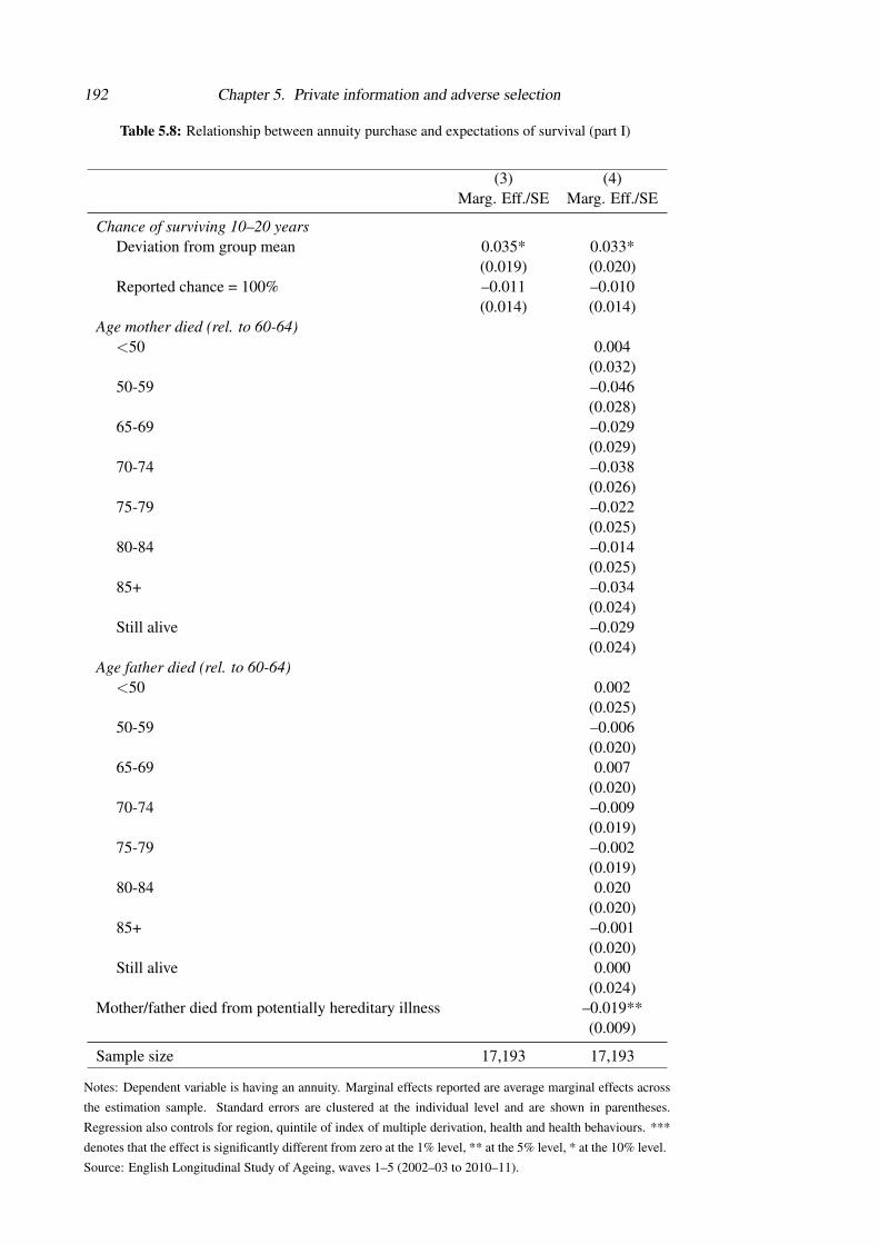
192 Chapter 5. Private information and adverse selection
Table 5.8: Relationship between annuity purchase and expectations of survival (part I)
(3) (4)Marg. Eff./SE Marg. Eff./SE
Chance of surviving 10–20 yearsDeviation from group mean 0.035* 0.033*
(0.019) (0.020)Reported chance = 100% –0.011 –0.010
(0.014) (0.014)Age mother died (rel. to 60-64)
<50 0.004(0.032)
50-59 –0.046(0.028)
65-69 –0.029(0.029)
70-74 –0.038(0.026)
75-79 –0.022(0.025)
80-84 –0.014(0.025)
85+ –0.034(0.024)
Still alive –0.029(0.024)
Age father died (rel. to 60-64)<50 0.002
(0.025)50-59 –0.006
(0.020)65-69 0.007
(0.020)70-74 –0.009
(0.019)75-79 –0.002
(0.019)80-84 0.020
(0.020)85+ –0.001
(0.020)Still alive 0.000
(0.024)Mother/father died from potentially hereditary illness –0.019**
(0.009)
Sample size 17,193 17,193
Notes: Dependent variable is having an annuity. Marginal effects reported are average marginal effects across
the estimation sample. Standard errors are clustered at the individual level and are shown in parentheses.
Regression also controls for region, quintile of index of multiple derivation, health and health behaviours. ***
denotes that the effect is significantly different from zero at the 1% level, ** at the 5% level, * at the 10% level.
Source: English Longitudinal Study of Ageing, waves 1–5 (2002–03 to 2010–11).

5.6. Results 193
Table 5.9: Relationship between annuity purchase and expectations of survival (part II)
(4) (5) (6)Marg. Eff./SE Marg. Eff./SE Marg. Eff./SE
Chance of surviving 10–20 yearsDeviation from group mean 0.033* 0.021 0.013
(0.020) (0.020) (0.020)Reported chance = 100% –0.010 –0.008 –0.000
(0.014) (0.014) (0.015)Mother/father died from potentially hereditary illness –0.019** –0.019** –0.018**
(0.009) (0.009) (0.009)Self-rated general health (rel. to good)
Excellent 0.009 0.004(0.012) (0.012)
Very good 0.002 –0.002(0.008) (0.008)
Fair –0.031*** –0.024**(0.011) (0.011)
Poor –0.045** –0.033*(0.019) (0.019)
Quintile of total wealth (rel. to quintile 3)Lowest –0.072***
(0.014)Quintile 2 –0.015
(0.012)Quintile 4 –0.003
(0.012)Highest 0.028**
(0.014)
Sample size 17,193 17,193 17,193Notes: Dependent variable is having an annuity. Marginal effects reported are average marginal effects across
the estimation sample. Standard errors are clustered at the individual level and are shown in parentheses.
Regression also controls for region, quintile of index of multiple derivation, health and health behaviours,
parents’ age at death. *** denotes that the effect is significantly different from zero at the 1% level, ** at the
5% level, * at the 10% level.
Source: English Longitudinal Study of Ageing, waves 1–5 (2002–03 to 2010–11).
Specification (5) adds indicators for individuals’ self-reported general health. Even
after controlling for detailed measures of objectively diagnosed health conditions and health
behaviours, individuals’ self-reported health is a significant predictor of annuity purchase.
The addition of this measure substantially attenuates the marginal effect of self-reported sur-
vival expectations (reducing it from 0.033 to 0.021, the latter being not statistically signific-
antly different from zero). This suggests that part of the private information that individuals
have is greater information about their current state of health. This is consistent with the
evidence reviewed by, for example, Idler and Benyamini (1997), that self-assessed health
is predictive of mortality even after controlling for a comprehensive set of other health and
socioeconomic variables.

194 Chapter 5. Private information and adverse selection
Idler and Benyamini (1997) suggest a number of reasons why self-assessed health
might have additional predictive power for future mortality. First, it may capture differences
in the severity of conditions that are not reflected in simple prevalence measures. Second,
self-assessed health may pick up as-yet-undiagnosed conditions. Third, believing that your
health is poor may be a direct cause of subsequent mortality – either because it motivates
people to invest less in health improving activities because they think their lifespan is limited
anyway, or because it contributes to depression which (it has been shown) can weaken the
immune system. It is beyond the scope of this paper to attempt to disentangle which of
these effects (or others) is important.
It would also be interesting to examine how the relationship between self-assessed
health and longevity differs if we were to account for the types of differences in response
scales that (among others) King et al. (2004), van Doorslaer and Lindeboom (2004) and
Grol-Prokopczyk, Freese, and Hauser (2011) have suggested are important. This could be
explored in future work.
Specification (6) adds indicators of which quintile of the wealth distribution the indi-
vidual falls in. This quintile is calculated based on the family’s total net wealth, including
private pension wealth but excluding wealth implicit in publicly funded pension promises.
The marginal effect of this variable is highly significant. This is one of the sources of poten-
tially ‘passive’ selection that Finkelstein and Poterba (2002) discuss. However, the results
in Table 5.9 suggest that it is not wholly passive, in the sense that wealth is correlated with
individuals’ expectations of their own survival – adding this regressor reduces the marginal
effect of respondents’ self-reported survival expectations from 0.021 to 0.013. It also re-
duces the marginal effect of the self-reported health status indicators.
It would be implausible for insurers to be able to elicit information on self-assessed
health from annuity purchasers. It would be unverifiable and the incentives for potential
purchasers to lie would be great. It might also be difficult for insurers to distinguish between
more and less wealthy individuals when setting annuity rates. It would not, for example,
be credible for insurers to offer lower prices to people purchasing smaller annuities since
someone wishing to buy a large annuity could always instead purchase multiple smaller
ones.17 While insurers could try to gather information on purchasers’ entire wealth port-
folios before they buy, it would be hard for them to verify this information and purchasers
17In practice, if anything, insurers tend to offer bulk discounts, suggesting that the additional costs of ad-ministering smaller annuities dominates any concern about those with more money being longer lived.

5.7. Riskiness and risk preferences 195
may not be happy to provide it.18
5.7 Riskiness and risk preferences
A number of papers have suggested that part of the explanation for the relationship seen
between insurance purchase and experience of adverse outcomes might be a result of un-
observed heterogeneity in risk preferences, as opposed to (only) differences in individuals’
riskiness. The results presented above show that, in the UK annuities market, there is at
least some active adverse selection. However, it is also interesting to know whether there
is an additional correlation between risk preferences and expectations of experiencing the
insured risk that might reinforce the positive correlation between holding an annuity and
being likely to survive to older ages.
In order to examine whether there is an additional correlation between risk preferences
and expectations of experiencing the insured risk, we ideally need to observe some indicator
of individuals’ preferences for risk-taking. For a subsample of ELSA respondents indicators
of this sort are available. A random sub-sample of respondents to the fifth wave were invited
to take part in an experimental module which aimed to gauge their time- and (financial)
risk-preferences. In this section I provide some tentative evidence on how financial risk
preferences relate to individuals’ perception of their own riskiness using data from this
experimental module. This provides a preliminary assessment of how private information
about financial risk preferences might add to the private information that individuals have
about their risk type that is not observed by insurers.
Figure 5.1 starts by comparing the distribution of self-assessed risk tolerance between
those who have higher and lower expectations of surviving. Individuals are grouped accord-
ing to how their expectations of survival compare to their age/sex group average.
Among men there is no clear relationship between expectations of survival and self-
assessed risk tolerance. Those who expect to live less long are more likely to say that they
‘avoid taking risks’ or to put themselves in the category just above this than are people who
expect to live for longer. The pattern across other responses is mixed.
Among women there is a clearer pattern, with those who expect to live for less long be-
ing more likely to put themselves in the bottom half of the available scale. 55% of women in
the lowest quintile of survival expectations ranked their willingness to take risk somewhere
18In an earlier version of this paper, I made use of the more detailed health measures from the wave 2 and4 nurse visits to examine whether any of these additional measures could mitigate the private information heldby respondents. However, the results of this exercise were inconclusive and so are not reported here.

196 Chapter 5. Private information and adverse selection
Figure 5.1: Self-assessed risk tolerance, by quintile of deviation between own and age/sex groupaverage expectations of survival
Notes: Sample is those aged 55–69 who completed the experimental risk module in ELSA wave 5. Individuals
are grouped according to how their self-reported expectation of surviving to a future age compares to the average
reported by other people of the same sex and age in wave 5.
Source: English Longitudinal Study of Ageing, wave 5 (2010–11).
between zero and five out of ten. This compares to 40% of those in the highest quintile of
survival expectations.
Figure 5.2 presents similar descriptive analysis but based on the measure of risk tol-
erance derived from the baseline experimental task. The ‘no risk’ group shown in Figure
5.2 are those who chose the lottery which gave them a guaranteed payout of 28. The ‘risk
loving’ group are those who chose the lottery that had a 50% chance of a pay-off of 2 and a
50% chance of a pay-off of 70.
The relationship between survival expectations and risk tolerance as measured by the
experimental task is unclear. Among men, those with the lowest survival expectations were
the most likely to take the no-risk or less risky options. However, among both men and
women, there appears to be a non-monotonic relationship between the likelihood of picking
the safe option and survival expectations: it is those in the middle of the distribution of
survival expectations who seem most likely to choose the riskier options.
It is difficult to draw concrete conclusions from this analysis, owing to the small sample
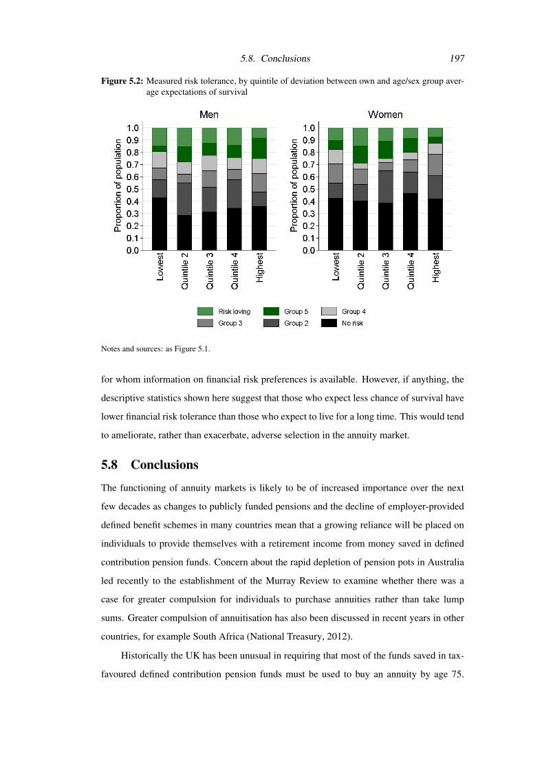
5.8. Conclusions 197
Figure 5.2: Measured risk tolerance, by quintile of deviation between own and age/sex group aver-age expectations of survival
Notes and sources: as Figure 5.1.
for whom information on financial risk preferences is available. However, if anything, the
descriptive statistics shown here suggest that those who expect less chance of survival have
lower financial risk tolerance than those who expect to live for a long time. This would tend
to ameliorate, rather than exacerbate, adverse selection in the annuity market.
5.8 Conclusions
The functioning of annuity markets is likely to be of increased importance over the next
few decades as changes to publicly funded pensions and the decline of employer-provided
defined benefit schemes in many countries mean that a growing reliance will be placed on
individuals to provide themselves with a retirement income from money saved in defined
contribution pension funds. Concern about the rapid depletion of pension pots in Australia
led recently to the establishment of the Murray Review to examine whether there was a
case for greater compulsion for individuals to purchase annuities rather than take lump
sums. Greater compulsion of annuitisation has also been discussed in recent years in other
countries, for example South Africa (National Treasury, 2012).
Historically the UK has been unusual in requiring that most of the funds saved in tax-
favoured defined contribution pension funds must be used to buy an annuity by age 75.

198 Chapter 5. Private information and adverse selection
This requirement has led to a much more developed annuity market existing in the UK
than elsewhere and consequently much of the academic work on the functioning of annuity
markets has focussed on the market in the UK. This paper continues that tradition.
Using detailed household microdata I have demonstrated that the adverse selection
found in this market is, at least in part, active. Individuals do appear to have private inform-
ation about their future longevity that is not fully captured by measures that are typically
used by insurers in pricing annuities. This private information appears to reflect partly
greater information about their current state of health and partly information about their
family history which is not observed by insurers. My analysis suggests comprehensive un-
derwriting on the basis of health (as is already used by some specialist providers) reduces
the degree of private information but insurers are likely to struggle to replicate fully indi-
viduals’ private information, even if they were to adopt more stringent underwriting criteria
than currently used.
One obvious question, in light of the evidence of adverse selection that I present here,
is what the efficiency cost of this might be. The evidence I present here is, unfortunately, not
sufficient to quantify the welfare effects of the adverse selection. As Einav, Finkelstein, and
Schrimpf (2007) show, the reduced form equilibrium relationship between annuity holding
and risk experience is not sufficient to infer the size of the efficiency cost of the asymmetric
information. In particular, the size of the distortion will depend on individuals’ elasticity of
demand for annuities and thus quantifying the efficiency cost requires knowledge not only
of risk types but also of risk preferences. Quantifying the efficiency costs would therefore
require further strong assumptions.
A further potential issue in knowing how private information on mortality risks affects
equilibrium pricing, choices and efficiency in the annuity market is raised by the analysis in
Chapter 4. That analysis shows that, while individuals do appear to have private information
about their relative risk (that is, how their survival chances compare to other people of the
same age and sex), they are not well-informed about the average mortality risks facing the
population. This suggests that the survival curve that individuals have in mind when they
evaluate the price offered to them by an insurer is different from the one that the insurer
uses in setting the price. An interesting avenue for future work would be to bring together
the insights from these two papers to understand better the equilibrium in this market.
While the UK government has historically had much stricter mandating of annuitisa-

5.8. Conclusions 199
tion than most other countries, these have recently been abolished – meaning that the UK
is somewhat swimming against the tide of reforms proposed elsewhere in the world. In
March 2014, the UK government unexpectedly announced that (from April 2015 onwards)
people would no longer be required to annuitise their pension fund by the age of 75. In-
stead individuals would be able to withdraw funds from their pension as and when they
wanted and simply face tax at their marginal rate on any income withdrawn. This reform
will potentially have a significant effect on the functioning of the UK annuity market. It
certainly had a significant immediate effect on some annuity providers – for example, the
share price of two specialist annuity providers (of enhanced and impaired life annuities) was
cut in half in the aftermath of the unexpected announcement by the Chancellor in the March
2014 Budget.19 It will be interesting and important to examine how the characteristics of
annuity purchasers and prices offered in the market change as individuals are given greater
flexibility about when and how to withdraw their accrued funds.
19See http://citywire.co.uk/new-model-adviser/news/partnership-drops-out-of-ftse-250-as-budget-bites/a754848?section=new-model-adviser.
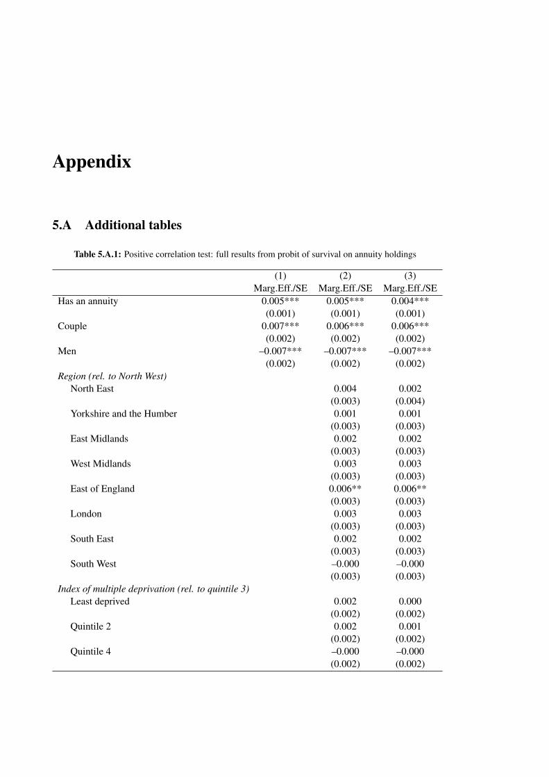
Appendix
5.A Additional tables
Table 5.A.1: Positive correlation test: full results from probit of survival on annuity holdings
(1) (2) (3)Marg.Eff./SE Marg.Eff./SE Marg.Eff./SE
Has an annuity 0.005*** 0.005*** 0.004***(0.001) (0.001) (0.001)
Couple 0.007*** 0.006*** 0.006***(0.002) (0.002) (0.002)
Men –0.007*** –0.007*** –0.007***(0.002) (0.002) (0.002)
Region (rel. to North West)North East 0.004 0.002
(0.003) (0.004)Yorkshire and the Humber 0.001 0.001
(0.003) (0.003)East Midlands 0.002 0.002
(0.003) (0.003)West Midlands 0.003 0.003
(0.003) (0.003)East of England 0.006** 0.006**
(0.003) (0.003)London 0.003 0.003
(0.003) (0.003)South East 0.002 0.002
(0.003) (0.003)South West –0.000 –0.000
(0.003) (0.003)Index of multiple deprivation (rel. to quintile 3)
Least deprived 0.002 0.000(0.002) (0.002)
Quintile 2 0.002 0.001(0.002) (0.002)
Quintile 4 –0.000 –0.000(0.002) (0.002)

5.A. Additional tables 201
Table 5.A.1 – continued from previous page(1) (2) (3)
Marg.Eff./SE Marg.Eff./SE Marg.Eff./SEMost deprived –0.002 –0.001
(0.003) (0.002)Smoking behaviour (rel. to non-smoker)
Ex-occasional smoker 0.000(0.002)
Ex-regular smoker –0.006***(0.001)
Current smoker –0.006***(0.002)
Body mass index (rel. to normal weight)Overweight 0.002
(0.002)Obese –0.001
(0.002)Doctor diagnosed health conditions
Heart condition/lung disease –0.012***(0.003)
Diabetes 0.004**(0.002)
Stroke –0.002(0.004)
Angina/hypertension –0.000(0.001)
Asthma 0.005***(0.001)
Arthritis –0.000(0.001)
Osteoporosis –0.007*(0.004)
Cancer/Alzheimer’s/Dementia/Parkinson’s –0.023***(0.005)
Psychological condition 0.001(0.002)
Sample size 17,193 17,193 17,193
Notes: Dependent variable is 2-year survival. Marginal effects reported are average marginal effects across
the estimation sample. Standard errors are clustered at the individual level and are shown in parentheses.
Regression also controls for region and quintile of index of multiple deprivation. *** denotes that the effect is
significantly different from zero at the 1% level, ** at the 5% level, * at the 10% level.
Source: English Longitudinal Study of Ageing, waves 1–5 (2002–03 to 2010–11).

202 Chapter 5. Private information and adverse selection
Table 5.A.2: Relationship between annuity purchase and expectations of survival (full results)
(1) (2) (3)Marg.Eff./SE Marg.Eff./SE Marg.Eff./SE
Couple –0.018 –0.022* –0.024**(0.012) (0.012) (0.012)
Men 0.075*** 0.076*** 0.071***(0.010) (0.010) (0.010)
Chance of surviving 10–20 yearsDeviation from group mean 0.054*** 0.046** 0.035*
(0.020) (0.019) (0.019)Reported chance = 100% –0.018 –0.014 –0.011
(0.014) (0.014) (0.014)Region (rel. to North West)
North East –0.054** –0.053**(0.024) (0.024)
Yorkshire and the Humber –0.034* –0.032(0.020) (0.020)
East Midlands –0.027 –0.026(0.021) (0.021)
West Midlands –0.020 –0.021(0.020) (0.020)
East of England –0.004 –0.002(0.020) (0.020)
London –0.063*** –0.062***(0.020) (0.020)
South East –0.019 –0.019(0.019) (0.019)
South West –0.015 –0.014(0.021) (0.021)
Index of multiple deprivation (rel. to quintile 3)Least deprived –0.002 –0.004
(0.015) (0.015)Quintile 2 –0.001 –0.001
(0.015) (0.014)Quintile 4 –0.003 –0.002
(0.016) (0.016)Most deprived –0.043** –0.040**
(0.017) (0.018)Smoking behaviour (rel. to non-smoker)
Ex-occasional smoker 0.009(0.021)
Ex-regular smoker 0.004(0.011)
Current smoker –0.016(0.015)
Body mass index (rel. to normal weight)Overweight 0.021*

5.A. Additional tables 203
Table 5.A.2 – continued from previous page(1) (2) (3)
Marg.Eff./SE Marg.Eff./SE Marg.Eff./SE(0.012)
Obese 0.003(0.013)
Doctor diagnosed health conditionsHeart condition/lung disease 0.007
(0.014)Diabetes –0.009
(0.016)Stroke –0.037
(0.026)Angina/hypertension –0.005
(0.010)Asthma –0.025*
(0.014)Arthritis 0.004
(0.010)Osteoporosis –0.034*
(0.020)Cancer/Alzheimer’s/Dementia/Parkinson’s 0.004
(0.016)Psychological condition –0.007
(0.015)
Sample size 17,193 17,193 17,193
Notes: Dependent variable is having an annuity. Marginal effects reported are average marginal effects across
the estimation sample. Regression also controlled for region and quintile of index of multiple derivation. Stand-
ard errors are clustered at the individual level and are shown in parentheses. *** denotes that the effect is sig-
nificantly different from zero at the 1% level, ** at the 5% level, * at the 10% level.
Source: English Longitudinal Study of Ageing, waves 1–5 (2002–03 to 2010–11).

204 Chapter 5. Private information and adverse selection
5.B Pricing annuities: underwriting practices in the UK
Annuity prices typically depend on the purchasers age and sex and, in the case of joint life
annuities, on their partners age and sex as well. Prices also often vary depending on the
purchasers address, with those living in more affluent areas facing higher prices than those
living in poorer areas.
In addition, some annuity products offer lower prices to those who can demonstrate
they are in poor health or engage in longevity decreasing activities – these are known as
impaired or enhanced life annuities. Enhanced life annuities are for smokers and those who
are over-weight. Impaired life annuities are for people with serious pre-existing medical
conditions. Health issues and medical conditions which would qualify for impaired life
annuities include, but are not limited to:20
• Blood Pressure (tablet controlled)
• Diabetes (In particular tablet controlled or Insulin dependent)
• Stroke
• High Cholesterol (tablet controlled)
• Asthma (controlled with medication)
• Cancer
• Smoking (manufactured cigarettes 10 per day for last 10 years, pipes, cigars, rolled
tobacco)
• Heart Attack (at any time)
• Atrial Fibrillation
• Angina (controlled with medication)
• Other Heart Conditions
• Organ replacements
• Bypass surgery and Angioplasties
20This list was taken from: http://www.nononsenseannuities.co.uk/impaired-life-annuities/.

5.B. Pricing annuities: underwriting practices in the UK 205
• Emphysema
• Rheumatoid Arthritis
• Parkinson’s Disease
• Alzheimer’s and Dementia
• Multiple Sclerosis
• COPD (chronic obstructive pulmonary disease), and other lung conditions
• Bronchitis
• Obesity (depending on height weight ratios)

206 Chapter 5. Private information and adverse selection
5.C ELSA nurse visitsAfter the second and fourth waves of ELSA (2004–05 and 2008–09), eligible respondents
also received a visit from a qualified nurse, who measured a number of aspects of their
health and also collected blood and saliva samples that were later analysed in a laboratory.
In wave 2, 89.3% of core sample members aged between 55 and 69 received a nurse visit;
in wave 4 the figure was 84.5%.
During the visit, the nurses took a number of measures of respondents’ physical condi-
tion and functioning. Specifically, measuring blood pressure, height, weight, waist circum-
ference, lung function, grip strength, balance and ability to stand from a chair repeatedly.
The nurse also collected blood and saliva samples that were later analysed in a laboratory
Standing height and weight were measured for all those who were able to stand for
sufficiently long. Weight was measured for those weighing no more than 130kg. If height
or weight could not be measured then an estimate was obtained from the respondent instead.
If the nurse thought the measurement was likely to be more than 2cm from the true figure
for height or more than 1 kg from the true figure for weight, it was marked as unreliable.
These height and weight measurements can be used to calculate BMI. These values can
then be grouped according to the World Health Organisation definitions of obesity. There
are some concerns about the BMI measure and recent evidence suggests that waist-to-height
ratio or waist circumference may be a better predictor of health problems than BMI (Ash-
well, Gunn, and Gibson, 2012). Respondents’ waist measurement was also recorded. In
the analysis presented in this paper, I only include controls for respondents’ BMI. I ex-
perimented with alternative specifications, controlling for BMI and/or waist circumference.
Waist circumference was found not to be predictive of survival over-and-above BMI and the
other included regressors.
Individuals are grouped according to whether they are obese (BMI>30), overweight
(BMI between 25 and 29.9), or normal weight (BMI under 25). Normal practice is also to
distinguish between those of normal weight and those who are underweight (usually defined
as BMI<18.5). However, there are so few people who are underweight in the ELSA sample
that I group these people with the normal weight group.
Chapter 6
Conclusions
The papers in this thesis address questions about individuals’ financial-related decisions
towards the end of working life and in early retirement using detailed household microdata.
The first half of the thesis looks the timing of retirement. The second half of the thesis looks
at how expectations of future survival affect economic behaviour.
The contributions of this thesis are four-fold. First, this thesis confirms that older men
in the United Kingdom (UK) are responsive to dynamic financial incentives to remain in
work at older ages and extends this finding to show that it also applies to women. Second,
I confirm earlier findings that increasing the early retirement age in a state pension scheme
has a significant effect on labour force participation of women. More importantly, I extend
the existing literature by showing that such an effect is seen even in a context (as in the UK)
where there are very limited financial incentives to retire at the early retirement age.
There has been a lot of focus in the economic literature (as there is in the first half of
this thesis) on how individuals respond to financial incentives around retirement. However,
the evidence presented in this thesis suggests that financial incentives alone cannot explain
how many people behave. Therefore, a fruitful avenue for future work would be to examine
the potential other mechanisms that may be at work. For example, over the next few years
more detailed household survey data (including panel data) should allow us to look at how
the date of exit from the labour market relates to the date at which women reach the early
retirement age and how this has been changing as the early retirement age for women has
increased.
The third contribution of the thesis is to show how systematic deviations of perceived
survival from life table values that are commonly assumed in dynamic models of behaviour
could help to explain some puzzling aspects of behaviour. In doing this I have also provided

208 Chapter 6. Conclusions
evidence on individuals’ expectations of survival in the UK, which is interesting in its own
right. This driver of individuals’ behaviour deserves some of the same attention that has
been devoted to understanding heterogeneity in discount rates. An interesting direction for
future work would be to build the estimates of individuals’ perceived survival curves that
I present into a structural dynamic model of behaviour and examine the implications for
estimated preference parameters, in particular discount rates and risk aversion.
The final contribution of this thesis is to the literature on adverse selection in insurance
markets. I show that there is a direct correlation between individuals’ expectation of survival
and the probability of purchasing an annuity, even after controlling for the increasingly
detailed underwriting criteria that are now used in pricing some annuities. This adds to
what had previously been established in the literature by showing that adverse selection
remains even after more extensive underwriting and that this adverse selection is active.
The analysis presented here is only possible with the unique combination of policy and data
availability that exists in the UK.
There is further work to be done to understand the nature of equilibrium in this market.
In particular, it would be interesting to give further thought to the nature of the equilibrium in
this market when it appears that buyers have private information but that buyers and sellers
hold systematically different beliefs about the risks facing the pool of potential purchasers.
There could also be value in learning more about individuals’ risk preferences to allow us to
estimate the welfare loss from adverse selection in this market. Understanding more about
the equilibrium in this market could be very important as many countries look to expand
the role of individually purchased annuities in providing longevity insurance. In the UK
the policy trend has been in the opposite direction, with new freedoms for people not to
purchase annuities. How will the market adapt to these changes, which may lead to even
greater selectivity?
The findings presented here provide many important lessons for policymakers, both in
the UK and beyond. First, Chapter 2 shows that changing the early retirement age can have
a significant effect on labour supply, even without associated strong financial incentives.
This suggests: (i) that this is an effective tool for increasing labour force participation of
older people, and (ii) that some of the financial disincentives to work past pension age that
exist in many countries’ systems could be removed without eliminating the effectiveness of
these focal ages in influencing labour force participation.

209
A second important lesson for policymakers is that, while individuals understand how
their potential longevity compares to others like them, they do not have a good sense of the
shape of survival curves. This has implications for how they will behave. Policymakers
could either adjust policy to help people make better decisions, given their lack of under-
standing – for example, introducing greater compulsion in pension saving to overcome the
problem that people tend to under-estimate their chances of surviving to younger old age –
or they could try to improve people’s knowledge or a combination of the two.
A third important lesson for policymakers is that active adverse selection occurs in
annuity markets. This is mitigated to some extent but not eliminated by more sophisticated
underwriting criteria. Understanding this and how it affects pricing and product offers in
this market will be important for policymakers in many countries that are looking to shift
the burden of providing longevity insurance from the public sector to individuals.
This thesis has made heavy use of data from a longitudinal study of the older household
population in England. The English Longitudinal Study of Ageing (ELSA), which was
modelled on the Health and Retirement Study in the United States, collects a wide range
of information about individuals’ characteristics, expectations, preferences and behaviour.
With ten years of data now available, it is becoming an increasingly invaluable tool for
helping to understand behaviour among this group. Chapters 3-5 demonstrate some of the
ways in which ELSA can be used. However, there is much of the data that remains under-
exploited. Work that is in progress to link ELSA data to administrative records from tax,
benefit and health authorities should also provide many new avenues for research, including
providing a better understanding of how individuals respond to policy and interact with
public institutions.


Bibliography
Adam, S. and D. Phillips (2013). An ex-ante analysis of the effects of the UK government’s
welfare reforms on labour supply in Wales. Report R75, Institute for Fiscal Studies.
Adams, J., E. Stamp, D. Nettle, E. M. G. Milne, and C. Jagger (2014). Socioeconomic pos-
ition and the association between anticipated and actual survival in older English adults.
Journal of Epidemiology and Community Health 68, 818–825.
Akerlof, G. A. (1970). The market for ‘lemons’: qualitative uncertainty and the market
mechanism. Quarterly Journal of Economics 84, 488–500.
Alan, S., J. Banks, S. Choi, T. F. Crossley, A. Rustichini, and N. Woods (2012). Risk and
time preferences in older persons: an experimental module in ELSA. mimeo.
Alan, S. and M. Browning (2010). Estimating intertemporal allocation parameters using
synthetic residual estimation. Review of Economic Studies 77, 1231–1261.
Anand, P., A. B. Kunnumakara, C. Sundaram, K. B. Harikumar, S. T. Tharakan, O. S. Lai,
B. Sung, and B. B. Aggarwal (2008). Cancer is a preventage disease that requires major
lifestyle changes. Pharmaceutical Research 25(9), 2097–2116.
Arellano, M. and J. Hahn (2007). Understanding bias in nonlinear panel models: some
recent developments. In R. Blundell, W. Newey, and T. Persson (Eds.), Advances in
Economics and Econometrics, pp. 381–409. Cambridge University Press.
Arnott, R. and J. Stiglitz (1988). The basic analytics of moral hazard. Scandinavian Journal
of Economics 90, 383–413.
Arthur, W. B. (1981). The economics of risks to life. American Economic Review 71,
54–64.

212 BIBLIOGRAPHY
Asch, B., S. J. Haider, and J. Zissimopoulos (2005). Financial incentives and retirement:
evidence from federal civil service workers. Journal of Public Economics 89(2), 427–
440.
Ashwell, M., P. Gunn, and S. Gibson (2012). Waist-to-height ratio is a better screening
tool than waist circumference and BMI for adult cardiometabolic risk factors: systematic
review and meta-analysis. Obesity Review 13(3), 275–286.
Association of British Insurers (2014). The UK annuity market: Facts and figures. Technical
report.
Atalay, K. and G. F. Barrett (2015). The impact of age pension eligibility age on retirement
and program dependence: evidence from an Australian experiment. Review of Economics
and Statistics 97(1), 71–87.
Attanasio, O. and C. Emmerson (2003). Mortality, health status and wealth. Journal of the
European Economic Association 1, 821–50.
Austen, J. (1811). Sense and Sensibility. Wordsworth Classics.
Baker, M. (2002). The retirement behavior of married couples: Evidence from the spouse’s
allowance. Journal of Human Resources 37(1), 1–34.
Banks, J., R. Blundell, and M. Casanova (2010). The dynamics of retirement behavior in
couples: Reduced-form evidence from England and the US.
Banks, J., R. Blundell, and S. Tanner (1998). Is there a retirement-savings puzzle? Amer-
ican Economic Review 88(4), 769–788.
Banks, J., T. F. Crossley, and S. Goshev (2007). Looking for private information in self-
assessed health. HEDG Working Paper 07/09, University of York.
Banks, J., C. Emmerson, and Z. Oldfield (2004). Not so brief lives: longevity expectations
and wellbeing in retirement, pp. 28–31. Economic and Social Research Council.
Banks, J., C. Emmerson, and G. Tetlow (2005). Estimating pension wealth of ELSA re-
spondents. IFS Working Paper WP05/09.

BIBLIOGRAPHY 213
Banks, J., C. Emmerson, and G. Tetlow (2007a). Better prepared for retirement? Using
panel data to improve wealth estimates of ELSA respondents. Working Paper WP07/12,
Institute for Fiscal Studies.
Banks, J., C. Emmerson, and G. Tetlow (2007b). Healthy retirement or unhealthy inactivity:
How important are financial incentives in explaining retirement? Conference Paper.
Banks, J., C. Emmerson, and G. Tetlow (2015). Effect of pensions and disability benefits
on retirement in the UK. In D. A. Wise (Ed.), Social Security programs and retirement
around the world: Disability insurance programs and retirement. University of Chicago
Press.
Banks, J. and Z. Oldfield (2007). Understanding pensions: cognitive function, numerical
ability and retirement saving. Fiscal Studies 28(2), 143–170.
Bassett, W. and R. Lumsdaine (2001). Probability limits: are subjective assessments ad-
equately accurate? Journal of Human Resources 36, 327–363.
Behagel, L. and D. Blau (2012). Framing Social Security reform: Behavioral responses to
changes in the full retirement age. American Economic Journal: Economic Policy 4(4),
41–67.
Belloni, M. and R. Alessie (2009). The importance of financial incentives on retirement
choices: New evidence for Italy. Labour Economics 16, 578–588.
Belloni, M. and R. Alessie (2013). Retirement choices in Italy: What an option value model
tells us. Oxford Bulletin of Economics and Statistics 75, 499–527.
Berkovec, J. and S. Stern (1991). Job exit behavior of older men. Econometrica 59(1),
189–210.
Bernheim, B. D. (1989). The timing of retirement: a comparison of expectations and real-
izations. In D. A. Wise (Ed.), The Economics of Aging. University of Chicago Press.
Bertrand, M., E. Duflo, and S. Mullainathan (2004). How much should we trust differences-
in-differences estimates? Quarterly Journal of Economics 119(1), 249–275.
Blau, D. M. (1998). Labor force dynamics of older married couples. Journal of Labor
Economics 16(3), 595–629.

214 BIBLIOGRAPHY
Blau, D. M. (2015). Pension, household saving, and welfare: A dynamic analysis of crowd
out. Quantitative Economics forthcoming.
Blau, D. M. and D. B. Gilleskie (2006). Health insurance and retirement of married couples.
Journal of Applied Econometrics 21, 935–953.
Bloom, D. E., D. Canning, M. Moore, and Y. Song (2007). The effect of subjective survival
probabilities on retirement and wealth in the united states. In R. Clark, A. Mason, and
N. Ogawa (Eds.), Population Aging, Intergenerational Transfers and the Macroeconomy.
Elgar Press.
Blundell, R., R. Crawford, E. French, and G. Tetlow (2016). Comparing retirement wealth
trajectories on both sides of the pond. Fiscal Studies forthcoming.
Blundell, R. and C. Emmerson (2007). Fiscal effects of reforming the UK state pension sys-
tem. In J. Gruber and D. Wise (Eds.), Social Security Programs and Retirement Around
the World. University of Chicago Press.
Blundell, R., C. Meghir, and S. Smith (2002). Pension incentives and the pattern of early
retirement. Economic Journal 112, C153–70.
Blundell, R., C. Meghir, and S. Smith (2004). Pension incentives and the pattern of re-
tirement in the United Kingdom. In J. Gruber and D. A. Wise (Eds.), Social Security
programs and retirement around the world: micro-estimation, pp. 643–689. University
of Chicago Press.
Borsch-Supan, A. and R. Schnabel (1999). Social security and retirement in Germany. In
J. Gruber and D. Wise (Eds.), Social Security and Retirement Around the World. Univer-
sity of Chicago Press.
Bottazzi, R., T. Jappelli, and M. Padula (2006). Retirement expectations, pension reforms,
and their impact on private wealth accumulation. Journal of Public Economics 90, 2187–
2212.
Bound, J. (1991). Self-reported versus objective measures of health in retirement models.
Journal of Human Resources 26, 106–138.
Bound, J., T. Stinebrickner, and T. Waidmann (2010). Health, economic resources and the
work decisions of older men. Journal of Econometrics 156, 106–129.
BIBLIOGRAPHY 215
Bozio, A., R. Crawford, C. Emmerson, and G. Tetlow (2010). Retirement outcomes and
lifetime earnings: descriptive evidence from linked ELSA–NI data. DWP Working Pa-
per 81.
Bozio, A., R. Crawford, and G. Tetlow (2010). The history of state pensions in the UK:
1948 to 2010. Briefing Note 105, Institute for Fiscal Studies.
Bozio, A., G. Laroque, and C. O’Dea (2013). Discount rate heterogeneity among older
households: A puzzle? Working Paper W13/02, Institute for Fiscal Studies.
Burstrom, B. and P. Fredlund (2001). Self-rated health: is it a good predictor of subsequent
mortality among adults in lower as well as in higher social classes? Epidemiology and
Community Health 55(11), 836–840.
Butler, J. S. and R. A. Moffitt (1982). A computationally efficient quadrature procedure for
the one-factor multinomial probit model. Econometrica 50, 761–764.
Cameron, A., J. Gelbach, and D. Miller (2008). Bootstrap-based improvements for infer-
ence with clustered errors. Review of Economics and Statistics 90(3), 414–427.
Cannon, E. and I. Tonks (2006). Survey of annuity pricing. Research Report 318, Depart-
ment for Work and Pensions.
Cannon, E. and I. Tonks (2011). Compulsory and voluntary annuities markets in the UK.
In O. Mitchell, J. Piggott, and N. Takayama (Eds.), Securing lifelong retirement income:
Global annuity markets and policy, pp. 171–194. Oxford University Press.
Cardon, J. H. and I. Hendel (2001). Asymmetric information in health insurance: Evidence
from the National Medical Expenditure Survey. RAND Journal of Economics 32(3),
408–427.
Cawley, J. and T. Philipson (1999). An empirical examination of information barriers to
trade in insurance. American Economic Review 89(4), 827–846.
Chan, S. and A. H. Stevens (2004). What you don’t know can’t help you: Pension know-
ledge and retirement decision-making. Review of Economics and Statistics 90(2), 253–
266.

216 BIBLIOGRAPHY
Chandler, D. and G. Tetlow (2014a). Employment of older people in England: 2012–13.
Briefing Note BN153, Institute for Fiscal Studies.
Chandler, D. and G. Tetlow (2014b). Retirement in the 21st century. Report R98, Institute
for Fiscal Studies.
Chiappori, P.-A., B. Jullien, B. Salanie, and F. Salanie (2006). Asymmetric information in
insurance: General testable implications. RAND Journal of Economics 37, 783–798.
Chiappori, P.-A. and B. Salanie (2000). Testing for asymmetric information in insurance
markets. Journal of Political Economy 108(1), 56–78.
Cohen, A. and P. Siegelman (2010). Testing for adverse selection in insurance markets.
Journal of Risk and Insurance 77(1), 39–84.
Coile, C. (2004). Retirement incentives and couples’ retirement decisions. The B.E. Journal
of Economic Analysis and Policy 4(1), 1–30.
Coile, C. and J. Gruber (2000). Social security and retirement. Working Paper 2000-11,
Center for Retirement Research at Boston College.
Coile, C. and J. Gruber (2007). Future Social Security wealth and the retirement decision.
Review of Economics and Statistics 89, 234–246.
Coppola, M. and C. Wilke (2014). At what age do you expect to retire? Retirement expect-
ations and increases in the statutory retirement age. Fiscal Studies 35(2), 165–188.
Crawford, R. (2012). ELSA pension wealth derived variables (waves 2 to 5): Methodology.
Technical report.
Crawford, R., S. Keynes, and G. Tetlow (2013). A single-tier pension: What does it really
mean? IFS Report R82.
Crawford, R. and G. Tetlow (2010). Employment, retirement and pensions. In J. Banks,
C. Lessof, J. Nazroo, N. Rogers, M. Stafford, and A. Steptoe (Eds.), Financial circum-
stances, health and well-being of the older population in England: The 2008 English
Longitudinal Study of Ageing (Wave 4). Institute for Fiscal Studies.

BIBLIOGRAPHY 217
Cribb, J., C. Emmerson, and G. Tetlow (2013). Incentives, shocks or signals: Labour supply
effects of increasing the female state pension age in the UK. Working Paper W13/03,
Institute for Fiscal Studies.
Daula, T. V. and R. A. Moffitt (1992). Estimating dynamic models of quit behavior: the
case of military reenlistment. Mimeo, United States Military Academy.
Dave, C., C. Eckel, C. Johnson, and C. Rojas (2010). Eliciting risk preferences: when is
simple better? Journal of Risk and Uncertainty 41, 219–243.
de Meza, D. and D. Webb (2001). Advantageous selection in insurance markets. RAND
Journal of Economics 32, 249–262.
De Nardi, M., E. French, and J. B. Jones (2010). Why do the elderly save? The role of
medical expenses. Journal of Political Economy 118, 39–75.
Department for Work and Pensions (2006). Security in retirement: Towards a new pensions
system. White Paper Cm 6841.
Department for Work and Pensions (2013). Family resources survey 2011/12. Technical
report.
Department for Work and Pensions (2014). The annual abstract of statistics for benefits,
national insurance contributions, and indices of prices and earnings. Technical report.
Disney, R., C. Meghir, and E. Whitehouse (1994). Retirement behaviour in Britain. Fiscal
Studies 15(1), 24–43.
Disney, R. and S. Smith (2002). The labour supply effect of the abolition of the earnings
rule for older workers in the United Kingdom. Economic Journal 112, C136–C152.
Dominitz, J. and C. Manski (1997). Using expectations data to study subjective income
expectations. Journal of the American Statistical Association 92, 855–867.
Donald, S. and K. Lang (2007). Inference with difference-in-differences and other panel
data. Review of Economics and Statistics 89(2), 221–233.
Eckel, C. and P. Grossman (2002). Sex differences and statistical stereotyping in attitudes
toward financial risk. Evolution and Human Behavior 23(4), 281–295.

218 BIBLIOGRAPHY
Eckel, C. and P. Grossman (2008). Forecasting risk attitudes: an experimental study us-
ing actual and forecast gamble choices. Journal of Economic Behavior and Organiza-
tion 68(1), 1–17.
Einav, L., A. Finkelstein, and P. Schrimpf (2007). The welfare cost of asymmetric inform-
ation: Evidence from the UK annuity market. Working Paper 13228, National Bureau of
Economc Research.
Elder, T. E. (2013). The predictive validity of subjective mortality expectations: Evidence
from the Health and Retirement Study. Demography 50, 569–589.
Engen, E. M., W. G. Gale, C. E. Uccello, C. D. Carroll, and D. I. Laibson (1999). The
adequacy of household saving. Brookings Papers on Economic Activity 1999(2), 65–187.
Fang, H. (2014). Insurance markets for the elderly. Working Paper 20549, National Bureau
of Economic Research.
Fields, G. and O. Mitchell (1984). The effects of social security reforms on retirement ages
and retirement incomes. Journal of Public Economics 25, 143–159.
Finkelstein, A. and K. McGarry (2006). Mutliple dimensions of private information from
the long-term care insurance market. American Economic Review 96(4), 938–958.
Finkelstein, A. and J. Poterba (2002). Selection effects in the United Kingdom individual
annuities market. Economic Journal 112(476), 28–50.
Finkelstein, A. and J. Poterba (2004). Adverse selection in insurance markets: Policyholder
evidence from the UK annuity market. Journal of Political Economy 112(1), 183–208.
Finkelstein, A. and J. Poterba (2014). Testing for adverse selection using ‘unused observ-
ables’ in insurance markets: Evidence from the UK annuity market. Journal of Risk and
Insurance 81(4), 709–734.
Fischer, I. (1930). The Theory of Interest. New York: MacMillan.
French, E. (2005). The effects of health, wealth, and wages on labour supply and retirement
behaviour. Review of Economic Studies 72, 395–427.
Friedman, B. M. and M. J. Warshawsky (1990). The cost of annuities: Implications for
saving behavior and bequests. Quarterly Journal of Economics 105(1), 135–154.

BIBLIOGRAPHY 219
Gan, L., M. Hurd, and D. McFadden (2004). Individual subjective survival curves. In D. A.
Wise (Ed.), Analyses in the Economics of Aging. University of Chicago Press.
Gan, L., M. Hurd, and D. McFadden (2005). Subjective mortality risk and bequests. Work-
ing Paper 10789, National Bureau of Economic Research.
Government Actuary’s Department (2003). Occupational pension schemes 2000: Eleventh
survey by the Government Actuary. Technical report.
Grol-Prokopczyk, H., J. Freese, and R. M. Hauser (2011). Using anchoring vigenttes to
assess group differences in general self-rated health. Journal of Health and Social Beha-
vior 52(2), 246–261.
Gruber, J. and D. A. Wise (Eds.) (2004). Social Security programs and retirement around
the world: Micro-estimation. Chicago: University of Chicago Press.
Gustman, A. and T. Steinmeier (1985). The 1983 social security reforms and labor supply
adjustments of older individuals in the long run. Journal of Labor Economics 3(2), 237–
253.
Gustman, A. L. and T. L. Steinmeier (2005). The social security early entitlement age in a
structural model of retirement and wealth. Journal of Public Economics 89, 441–463.
Hamermesh, D. S. (1985). Expectations, life expectancy and economic behavior. Quarterly
Journal of Economics 100, 389–408.
Hamermesh, D. S. and F. W. Hamermesh (1983). Does perception of life expectancy reflect
health knowledge? American Journal of Public Health 73, 911–914.
Hanel, B. and R. T. Riphahn (2012). The timing of retirement: New evidence from Swiss
female workers. Labour Economics 19, 718–728.
He, D. (2009). The life insurance market: Asymmetric information revisited. Journal of
Public Economics 93, 1090–1097.
Heckman, J. (1979). Sample selection bias as a specification error. Econometrica 47, 153–
161.
Hemenway, D. (1990). Propitious selection. Quarterly Journal of Economics 105(4), 1063–
1069.

220 BIBLIOGRAPHY
Hendel, I. and A. Lizzeri (2003). The role of commitment in dynamic contracts: Evidence
from life insurance. Quarterly Journal of Economics 118(1), 299–327.
Hendricks, L. (2007). How important is discount rate heterogeneity for wealth inequality.
Journal of Economic Dynamics and Control 31, 3042–3068.
Hubbard, R. G., J. Skinner, and S. P. Zeldes (1995). Precautionary saving and social insur-
ance. Journal of Political Economy 103(2), 360–399.
Hurd, M. (1990). The joint retirement decision of husbands and wives. In D. A. Wise (Ed.),
Issues in the Economics of Aging, pp. 231–258. University of Chicago Press.
Hurd, M. and K. McGarry (1995). Evaluation of the subjective probabilities of survival in
the Health and Retirement Study. Journal of Human Resources 30, S268–S292.
Hurd, M. and K. McGarry (2002). The predictive validity of subjective probabilities of
survival. Economic Journal 112, 966–985.
Hurd, M., J. P. Smith, and J. Zissimopoulos (2004). The effects of subjective survival on
retirement and social security claiming. Journal of Applied Econometrics 19, 761–775.
Idler, E. L. and Y. Benyamini (1997). Self-rated health and mortality: A review of twenty-
seven community studies. Journal of Health and Social Behaviour 38(1), 21–37.
Jullien, B., B. Salanie, and F. Salanie (2007). Screening risk-averse agents under moral
hazard. Economic Theory 30, 151–169.
Juster, F. T. (1966). Consumer buying intentions and purchase probabilitie: an experiment
in survey design. Journal of the American Statistical Association 61.
Kathiresan, S. and D. Srivastava (2012). Genetics of human cardiovascular disease.
Cell 148(6), 1242–1257.
Khwaja, A., F. Sloan, and S. Chung (2007). The relationship between individual expecta-
tions and behaviors: Mortality expectations and smoking decisions. Journal of Risk and
Uncertainty 35, 179–201.
King, G., C. J. L. Murray, J. A. Salomon, and A. Tandom (2004). Enhancing the validity
and cross-cultural comparability of measurement in survey research. American Political
Science Review 98(1), 567–583.

BIBLIOGRAPHY 221
Kopczuk, W. and J. Song (2008). Stylized facts and incentive effects relating to claiming of
retirement benefits based on Social Security Administration data. Working Paper 2008-
200, Michigan Retirement Research Centre.
Lalive, R. and S. Staubli (2014). How does raising women’s full retirement age affect labor
supply, income, and mortality: evidence from Switzerland. Conference paper, Retirement
Research Consortium.
Lazear, E. P. (1979). Why is there mandatory retirement? Journal of Political Eco-
nomy 87(6), 1261–1284.
Lew, E. A. and L. Garfinkel (1987). Differences in mortality and longevity by sex, smoking
habits and health status. Journal of the Society of Actuaries 39, 107–130.
Liang, K. and S. Zeger (1986). Longitudinal data analysis using generalized linear models.
Biometrika 73(1), 13–22.
Lowe, J. (2014). Whither UK annuities? Report, International Longevity Centre.
Ludwig, A. and A. Zimper (2013). A parsimonious model of subjective life expectancy.
Theory 75, 519–541.
Lumsdaine, R., J. Stock, and D. Wise (1996). Why are retirement rates so high at age 65?
In D. Wise (Ed.), Advances in the Economics of Aging. University of Chicago Press.
Lumsdaine, R. L., J. H. Stock, and D. A. Wise (1992). Three models of retirement: Com-
putational complexity versus predictive validity. In D. A. Wise (Ed.), Topics in the Eco-
nomics of Aging, pp. 21–60. University of Chicago Press.
Manski, C. (2004). Measuring expectations. Econometrica 72, 1329–1376.
Marciniak, S. J. and D. A. Lomas (2010). Pulmonary Disorders: Hereditary. John Wiley
& Sons, Ltd.
Mastrobuoni, G. (2009). Labor supply effects of the recent social security benefit cuts:
Empirical estimates using cohort discontinuities. Journal of Public Economics 93, 1224–
1233.
McCarthy, D. and O. S. Mitchell (2003). International adverse selection in life insurance
and annuities. Working Paper 9975, National Bureau of Economic Research.

222 BIBLIOGRAPHY
Meghir, C. and E. Whitehouse (1997). Labour market transitions and retirement of men in
the uk. Journal of Econometrics 79, 327–354.
Michaud, P.-C. (2003). Joint labour supply dynamics of older couples. Discussion Paper
832, IZA.
Modigliani, F. and R. Brumberg (1954). Utility analysis and the consumption function: an
interpretation of cross-section data. In K. Kurihara (Ed.), Post-Keynsian Economics, pp.
388–436. Rutgers UP.
Moulton, B. (1990). An illustration of a pitfall in estimating the effects of aggregate vari-
ables on micro units. Review of Economics and Statistics 72(2), 334–338.
National Centre for Social Research (2012). English Longitudinal Study of Ageing: Wave
five interview questionnaire. Survey documentation.
National Treasury (2012). Preservation, portability and governance for retirement funds.
Technical discussion paper, South African National Treasury.
O’Donnell, O., F. Teppa, and E. van Doorslaer (2008). Can subjective survival expectations
explain retirement behaviour? Working Paper 188, DNB.
Office for National Statistics (2011). Trends in life expectancy by the national statistics
socio-economic classification 1982–2006. Statistical Bulletin.
Office for National Statistics (2012). Interim life tables, England, 1980–82 to 2008–10.
Technical report.
Pensions Policy Institute (2013). The pensions primer: A guide to the UK pension system
– historical annex. Technical report.
Poterba, J. M., S. F. Venti, and D. A. Wise (2011). Family status transitions, latent health,
and the post-retirement evolution of assets. In D. A. Wise (Ed.), Explorations in the
Economics of Aging. University of Chicago Press.
Poterba, J. M., S. F. Venti, and D. A. Wise (2013). Health, retirement, and the post-
retirement evolution of household assets. Working Paper 18695, National Bureau of
Economic Research.

BIBLIOGRAPHY 223
Rothschild, C. G. (2009). Adverse selection in annuity markets: Evidence from the British
Life Annuity Act of 1808. Journal of Public Economics 93, 776–784.
Rothschild, M. and J. Stiglitz (1976). Equilibrium in competitve insurance markets: Essay
on the economics of imperfect information. Quarterly Journal of Economics 90, 630–
649.
Rust, J. and C. Phelan (1997). How Social Security and Medicare affect retirement behavior
in a world of incomplete markets. Econometrica 65(4), 781–831.
Rust, J. P. (1989). A dynamic programming model of retirement behavior. In D. A. Wise
(Ed.), The Economics and Aging, pp. 359–404. University of Chicago Press.
Samwick, A. (1998). Discount rate heterogeneity and social security reform. Journal of
Development Economics 57, 117–146.
Scholz, J. K., A. Seshadri, and S. Khitatrakun (2006). Are Americans saving ‘optimally’
for retirement? Journal of Political Economy 114(4), 607–643.
Smith, J. P. (1998). Socioeconomic status and health. American Economic Review 88,
192–196.
Stancanelli, E. (2012). Spouses’ retirement and hours outcomes: Evidence from twofold
regression discontinuity with differences-in-differences. Discussion Paper 6791, IZA.
Staubli, S. and J. Zweimuller (2013). Does raising the retirement age increase employment
of older workers? Journal of Public Economics 108, 17–32.
Stock, J. H. and D. A. Wise (1990). Pensions, the option value of work, and retirement.
Econometrica 58, 1151–1180.
van der Klaauw, W. and K. I. Wolpin (2008). Social Security and the retirement and savings
behavior of low-income households. Journal of Econometrics 145, 21–42.
van Doorslaer, E. and U.-G. Gerdtham (2003). Does inequality in self-assessed health
predict inequality in survival by income? Evidence from Swedish data. Social Science
and Medicine 57(9), 1621–1629.
van Doorslaer, E. and M. Lindeboom (2004). Cut-point shifts and index shift in self-
reported health. Journal of Health Economics 23, 1083–1099.
224 BIBLIOGRAPHY
Wise, D. A. (Ed.) (2015). Social Security programs and retirement around the world: dis-
ability insurance programs and retirement. University of Chicago Press.
Wooldridge, J. M. (2002). Econometric analysis of cross section and panel data. Mas-
sachusetts Institute of Technology.
Wupperman, A. (2010). Empirical Essays in Health and Education Economics. Ph. D.
thesis, Ludwigs-Maximilians-Universitat, Munich.
Yaari, M. E. (1965). Uncertain lifetime, life insurance, and the theory of the consumer.
Review of Economic Studies 32, 137–150.