
Essays on Sustainability and Poverty
123
Essays on Sustainability and Poverty Tianshu Li Shenyang, China Master of Economics, University of Tokyo, 2010 M.A. Economics, University of Virginia, 2012 A Dissertation presented to the Graduate Faculty of the University of Virginia in Candidacy for the Degree of Doctor of Philosophy Department of Economics University of Virginia May, 2016
Transcript of Essays on Sustainability and Poverty

Essays on Sustainability and Poverty
Tianshu LiShenyang, China
Master of Economics, University of Tokyo, 2010
M.A. Economics, University of Virginia, 2012
A Dissertation presented to the Graduate Faculty
of the University of Virginia in Candidacy for the Degree of
Doctor of Philosophy
Department of Economics
University of Virginia
May, 2016

UNIVERSITY OF VIRGINIA
AbstractDepartment of Economics
Doctor of Philosophy
by Tianshu Li
The three chapters of my dissertation mainly study two related issues. Chapter 1 focuses
on the sustainability problem concerning inter-generational welfare disparity, and Chap-
ters 2 and 3 focus on the poverty problem concerning cross-sectional welfare disparity.
In Chapter 1, “Protecting the Breadbasket with Trees? The Effect of the Great Plains
Shelterbelt Project on Agricultural Production”, I empirically estimate the short- and
long-term effects of planting windbreak trees on agricultural revenue by analyzing the
Great Plains Shelterbelt Project implemented in 1935-1942 in the US. In order to address
the endogeneity problem in the location choice of tree planting, I use a 100-mile-wide
belt-shaped shelterbelt zone designated by the program as the instrument. My estimates
show that a 10% increase in shelterbelt coverage in a county leads to a 7-10% increase in
agricultural revenue. This increase is attributable to animal products rather than crops,
and farmers in the treated counties were more likely to switch from cropland to pasture,
especially for cattle ranching. In addition, I find heterogeneous effects by levels of soil
erosion caused by the 1930s Dust Bowl. The regions with lower levels of soil erosion
benefit from shelterbelts, whereas highly eroded regions do not.
In Chapter 2, “Poverty Targeting and Income Distribution: Evidence from China’s Na-
tional Designated Poor Counties”, we study the impact of poverty targeting on house-
hold income using three natural experiments through adjustments in China’s National
Designated Poor Counties program between 1988 and 2008, in combination with agri-
cultural promotion policies. With difference-in-difference analyses, we consistently find
that when government publicity promoted agriculture, agricultural income of households
in newly designated counties increased, while non-agricultural income declined. In ad-
dition, we examine the redistributive effects of the policy: an increase in agricultural
income benefited the rich rather than the poor while a decline in non-agricultural in-
come (mainly wage income) affected both the rich and the poor. More interestingly,
once the designation ceased, people received less income from both agricultural and
non-agricultural sources. Overall, this regional targeting policy led to an inter-sectoral

ii
distortion favoring agricultural production and provided no evidence that its policy
package benefited the poorest households in the poor county.
In Chapter 3, “The Unintended Consequences of Employment-Based Safety Net Pro-
grams”, we examine the consequences of increasing rural employment opportunities for
the human capital accumulation of children in rural areas as employment guarantee
program are widely used as an anti-poverty lever in the developing world. We evaluate
the impact of India’s flagship Mahatma Gandhi National Rural Employment Guaran-
tee Scheme (MGNREGA) on school enrollment. We exploit the timing of roll-out of
MGNREGA across Indian districts and find that introduction of MGNREGA results in
lower relative enrollment in treated districts. Using nationally representative employ-
ment data, we find consistent evidence indicating an increase in child labor highlighting
the unintentional perverse effects of the employment guarantee schemes.

Acknowledgements
Pursuing a Ph.D. degree in economics has been an enlightening, inspiring, and challeng-
ing experience. As one of my most important accomplishment, it would not have been
possible without the guidance, encouragement, and support from my advisors, family,
and friends.
The exposure to economics that I received from Yasuyuki Sawada, Motoshige Itoh,
and R. Anton Brown at the University of Tokyo has opened my door to this engaging
field. Moreover, it is my advisors at the University of Virginia that have enlightened me
with the thoughts, tools, and consciousness as an economist. Leora Friedberg provides
me tirelessly advise and always had an open door when I needed help. Sheetal Sekhri
entrusted me with many opportunities and has been a nurturing teacher to my academic
career. Peter Debaere has helped me broaden my scope in viewing economic problems
and provides fruitful collaboration and devoted mentorship. Jay Shimshack gives me
altruistic help supporting my research and career, and I always cherish his insightful
opinion and judgment. I also sincerely appreciate Molly Lipscomb, Sarah Turner, Heidi
Schramm, Sisir Debnath, Sangui Wang, Kelsey Jack, Dennis Yang, Wallace Huffman,
David Hennessy, Kathy Baylis, Ken Leonard, Albert Park, Xiaohuan Lan, as well as
other professors and scholars who shared their wisdom over these years. In addition,
I would like to thank the Research Center for Rural Economy in China for providing
access to data. I am also grateful for financial support from the Center for International
Studies, the Steer Family Endowed Fund, and the Department of Economics at the
University of Virginia.
I am fortunate to have been through this process together with all my friends at the
University of Virginia, including Xiuchang Yang, Ce Shi, Li Zhang, Scott Laughery,
Tianying He, Xiaping Tang, Jimiao Du, Xian Zhou, Shuhui Chen, Xiaoyuan Wang, as
well as many others that I met in Charlottesville. Their company has made the burden
on the road seem much lighter.
I also appreciate a lifetime of encouragement and unabated support from my parents.
Ultimately, it is my wife, Zhengzheng, who has stood by me throughout this process.
Her love, comfort, and trust has kept me motivated and committed to my work and life.
I dedicate this dissertation to her.
iii

Contents
Abstract i
Acknowledgements iii
List of Figures vi
List of Tables vii
1 Protecting the Breadbasket with Trees? The Effect of the Great PlainsShelterbelt Project on Agricultural Production 1
1.1 Introduction . . . . . . . . . . . . . . . . . . . . . . . . . . . . . . . . . . . 1
1.2 Contextual Information . . . . . . . . . . . . . . . . . . . . . . . . . . . . 4
1.2.1 Background of the Program . . . . . . . . . . . . . . . . . . . . . . 4
1.2.2 Trade-offs of the Shelterbelts . . . . . . . . . . . . . . . . . . . . . 5
1.3 Conceptual Framework . . . . . . . . . . . . . . . . . . . . . . . . . . . . . 6
1.4 Data . . . . . . . . . . . . . . . . . . . . . . . . . . . . . . . . . . . . . . . 7
1.5 Estimation Strategy . . . . . . . . . . . . . . . . . . . . . . . . . . . . . . 8
1.5.1 Endogeneity Concerns and the Instrumental Variable . . . . . . . . 8
1.5.2 Validity of the Instrumental Variable . . . . . . . . . . . . . . . . . 9
1.5.3 Estimation Procedure . . . . . . . . . . . . . . . . . . . . . . . . . 10
1.6 Results . . . . . . . . . . . . . . . . . . . . . . . . . . . . . . . . . . . . . . 11
1.6.1 Main Results . . . . . . . . . . . . . . . . . . . . . . . . . . . . . . 11
1.6.2 Additional Results about Mechanisms . . . . . . . . . . . . . . . . 12
1.6.3 Results by Different Erosion Categories . . . . . . . . . . . . . . . 13
1.7 Robustness Checks . . . . . . . . . . . . . . . . . . . . . . . . . . . . . . . 14
1.7.1 The East and the West of the Shelterbelt Zone . . . . . . . . . . . 14
1.7.2 Alternative Channel: Labor and Capital Input . . . . . . . . . . . 15
1.7.3 Alternative Channel: Irrigation . . . . . . . . . . . . . . . . . . . . 15
1.7.4 Alternative Channel: the Great Plains Conservation Program andOther Programs . . . . . . . . . . . . . . . . . . . . . . . . . . . . 16
1.8 Conclusion . . . . . . . . . . . . . . . . . . . . . . . . . . . . . . . . . . . 17
iv

Contents v
2 Poverty Targeting and Income Distribution: Evidence from China’sNational Designated Poor Counties(co-authored with Sangui Wang) 39
2.1 Introduction . . . . . . . . . . . . . . . . . . . . . . . . . . . . . . . . . . . 39
2.2 Contextual Information . . . . . . . . . . . . . . . . . . . . . . . . . . . . 42
2.2.1 Background of the Targeting Program . . . . . . . . . . . . . . . . 42
2.2.2 Criteria for the Designation of the Poor Counties . . . . . . . . . . 43
2.3 Model . . . . . . . . . . . . . . . . . . . . . . . . . . . . . . . . . . . . . . 44
2.4 Data . . . . . . . . . . . . . . . . . . . . . . . . . . . . . . . . . . . . . . . 47
2.5 Estimation Strategy . . . . . . . . . . . . . . . . . . . . . . . . . . . . . . 48
2.5.1 Three Experiments and the Selection Problem . . . . . . . . . . . 48
2.5.2 Estimation Procedure . . . . . . . . . . . . . . . . . . . . . . . . . 49
2.6 Results . . . . . . . . . . . . . . . . . . . . . . . . . . . . . . . . . . . . . . 50
2.6.1 Inter-sectoral Effect under the Experiments . . . . . . . . . . . . . 50
2.6.2 Within County Distributional Effect . . . . . . . . . . . . . . . . . 52
2.6.3 Overall Effect and the Effect of Political Background . . . . . . . . 53
2.7 Robustness Checks . . . . . . . . . . . . . . . . . . . . . . . . . . . . . . . 54
2.8 Conclusion . . . . . . . . . . . . . . . . . . . . . . . . . . . . . . . . . . . 56
3 The Unintended Consequences of Employment-Based Safety Net Pro-grams(co-authored with Sheetal Sekhri) 74
3.1 Introduction . . . . . . . . . . . . . . . . . . . . . . . . . . . . . . . . . . . 74
3.2 Contextual Information . . . . . . . . . . . . . . . . . . . . . . . . . . . . 78
3.2.1 Background-National Rural Employment Guarantee Act . . . . . 78
3.2.2 Roll-out of the MGNREGA Program . . . . . . . . . . . . . . . . . 79
3.3 Conceptual Framework . . . . . . . . . . . . . . . . . . . . . . . . . . . . . 80
3.4 Data . . . . . . . . . . . . . . . . . . . . . . . . . . . . . . . . . . . . . . . 81
3.5 Estimation Strategy . . . . . . . . . . . . . . . . . . . . . . . . . . . . . . 82
3.5.1 Roll-out and Selection . . . . . . . . . . . . . . . . . . . . . . . . . 83
3.5.2 Estimation Procedure . . . . . . . . . . . . . . . . . . . . . . . . . 84
3.6 Results . . . . . . . . . . . . . . . . . . . . . . . . . . . . . . . . . . . . . . 85
3.6.1 Overall Enrollment . . . . . . . . . . . . . . . . . . . . . . . . . . . 85
3.6.2 Effects on Enrollment by Type of Schools . . . . . . . . . . . . . . 86
3.6.3 Schooling Outcomes . . . . . . . . . . . . . . . . . . . . . . . . . . 86
3.6.4 Mechanisms . . . . . . . . . . . . . . . . . . . . . . . . . . . . . . . 87
3.7 Robustness Checks and Sensitivity Analysis . . . . . . . . . . . . . . . . . 88
3.8 Alternative Channels . . . . . . . . . . . . . . . . . . . . . . . . . . . . . . 89
3.8.1 Other Programs . . . . . . . . . . . . . . . . . . . . . . . . . . . . 89
3.8.2 Growth and Demand for Private Schools . . . . . . . . . . . . . . . 90
3.8.3 Migration and Population Changes . . . . . . . . . . . . . . . . . . 90
3.9 Caveats . . . . . . . . . . . . . . . . . . . . . . . . . . . . . . . . . . . . . 91
3.10 Conclusion . . . . . . . . . . . . . . . . . . . . . . . . . . . . . . . . . . . 91

List of Figures
1.1 100-mile-wide Belt and Counties in Treatment and Control Groups . . . . 22
1.2 The Effect of Windbreaks on Wind Velocity . . . . . . . . . . . . . . . . . 23
1.3 An Example of Shelterbelt Planting . . . . . . . . . . . . . . . . . . . . . 24
1.4 The Pre-treatment Trends for Agricultural Revenue per Acre . . . . . . . 25
1.5 The Location of the Ogallala Aquifer and the 100-mile-wide Belt . . . . . 26
1.6 Designated Counties under the Great Plains Conservation Program . . . . 27
2.1 Treated and Selected Control Counties in Experiment I . . . . . . . . . . 59
2.2 Treated and Selected Control Counties in Experiment II . . . . . . . . . . 60
2.3 Treated and Selected Control Counties in Experiment III . . . . . . . . . 61
3.1 Districts in Different Phases of NREGA . . . . . . . . . . . . . . . . . . . 98
3.2 Total Enrollment by Phases . . . . . . . . . . . . . . . . . . . . . . . . . . 99
3.3 Total Number of Schools by Phases . . . . . . . . . . . . . . . . . . . . . . 99
3.4 Year Wise Impact . . . . . . . . . . . . . . . . . . . . . . . . . . . . . . . 100
3.5 Phase Wise Expansion in Different Types of Schools . . . . . . . . . . . . 101
vi

List of Tables
1.1 Comparison of Treated and Control Counties in 1930 (weighted by farm-land area) . . . . . . . . . . . . . . . . . . . . . . . . . . . . . . . . . . . . 28
1.2 OLS and 2SLS Regression Results on Farm Revenue per Acre . . . . . . . 29
1.3 Effect of Shelterbelt-planting on Other Related Outcome Variables (2SLS) 30
1.4 Effect of Shelterbelt-planting on Major Crops and Livestock (2SLS) . . . 31
1.5 2SLS Regression Results on Farm Revenue by Soil-erosion Level . . . . . 32
1.6 East versus West on Farm Revenue per Acre: log(Total revenue per acre) 33
1.7 Effect of Shelterbelt-planting on Labor and Capital (2SLS) . . . . . . . . 34
1.8 Effect of Shelterbelt-planting and the Great Plains Conservation Program 35
1.9 Comparison of Treated and Control Counties in 1930 by Different Cutoff . 36
1.10 Effect of Shelterbelt-planting Comparing Counties along the Eastern Bound-ary of the Belt . . . . . . . . . . . . . . . . . . . . . . . . . . . . . . . . . 37
1.11 Effect of Shelterbelt-planting Comparing Counties along the Western Bound-ary of the Belt . . . . . . . . . . . . . . . . . . . . . . . . . . . . . . . . . 38
2.1 Summary Statistics by Treated and Control Groups . . . . . . . . . . . . 62
2.2 Seemingly Unrelated Regressions for NDP Counties on Agricultural andSelf-employed Industrial Income . . . . . . . . . . . . . . . . . . . . . . . . 63
2.3 Seemingly Unrelated Regressions for NDP Counties on Agricultural andNon-agricultural Income . . . . . . . . . . . . . . . . . . . . . . . . . . . . 64
2.4 Quantile Regression Results for the Treatment in 1993: Newly Designatedvs Never Designated . . . . . . . . . . . . . . . . . . . . . . . . . . . . . . 65
2.5 Quantile Regression Results for the Treatment in 2001: Newly Designatedvs Never Designated . . . . . . . . . . . . . . . . . . . . . . . . . . . . . . 66
2.6 Quantile Regression Results for the Treatment in 2001: Ceased Designa-tion vs Always Designated . . . . . . . . . . . . . . . . . . . . . . . . . . . 67
2.7 Quantile Regression Results on Household Gross Income . . . . . . . . . . 68
2.8 OLS Regressions for Households with Political Background for the Treat-ment Groups of National Designated Poor Counties . . . . . . . . . . . . . 69
2.9 Seemingly Unrelated Regressions for Placebo Test I on Agricultural andSelf-employed Industrial Income . . . . . . . . . . . . . . . . . . . . . . . . 70
2.10 Seemingly Unrelated Regressions for Placebo Test I on Agricultural andNon-agricultural Income . . . . . . . . . . . . . . . . . . . . . . . . . . . . 71
2.11 Seemingly Unrelated Regressions for Placebo Test II on Agricultural andSelf-employed Industrial Income . . . . . . . . . . . . . . . . . . . . . . . . 72
vii

List of Tables viii
2.12 Seemingly Unrelated Regressions for Placebo Test II on Agricultural andNon-agricultural Income . . . . . . . . . . . . . . . . . . . . . . . . . . . . 73
3.1 Summary Statistics Outcome variables (All phases, all years) . . . . . . . 102
3.2 Summary Statistics- Outcome Variables by NREGA Phases . . . . . . . . 103
3.3 Comparison of District Level Characteristics across NREGA Phases . . . 104
3.4 The Impact of Introduction of NREGA on Enrollment (2005-08) . . . . . 105
3.5 Heterogneous Impact of the Introduction of NREGA on Enrollment (2005-08) . . . . . . . . . . . . . . . . . . . . . . . . . . . . . . . . . . . . . . . . 106
3.6 The Impact of the Introduction of NREGA on Performance Outcomes(2005-08) . . . . . . . . . . . . . . . . . . . . . . . . . . . . . . . . . . . . 107
3.7 Linear Probability Regression Results on Child Labor (Age: 5 - 15) . . . . 108
3.8 The Impact of the Introduction of NREGA on Enrollment (2005-08) Con-trolling Pre-trends from 2003 to 2005 . . . . . . . . . . . . . . . . . . . . . 109
3.9 Placebo Test for Child Labor Using Pre-period Data (Age: 5 - 15) . . . . 110
3.10 The Impact of Introduction of NREGA on Enrollment (2005-08) Exclud-ing States for Which 2003-2005 Data Is Unavailable . . . . . . . . . . . . 111
3.11 Heterogeneous Impact of the Introduction of NREGA on Enrollment(2005-08) Excluding States for Which 2003-2005 Data Is Unavailable . . . 112
3.12 The Impact of the Introduction of NREGA on Additional PerformanceOutcomes (2005-08) . . . . . . . . . . . . . . . . . . . . . . . . . . . . . . 113

Dedicated to Princess Sophie for her birthday and the 2ndanniversary of our marriage. . .
ix

Chapter 1
Protecting the Breadbasket with
Trees? The Effect of the Great
Plains Shelterbelt Project on
Agricultural Production
1.1 Introduction
Wind erosion degrades the environment and is detrimental for agricultural production. It
widely affects many arid and semi-arid areas and is a global policy concern (Toy, Foster,
and Renard, 2002). One of the most famous examples, the 1930s American Dust Bowl,
is estimated to have persistently decreased annual agricultural revenue and farmland
value by 20-30% from the 1940s to the 1990s in highly eroded Great Plains areas in the
US (Hornbeck, 2012). Historically, several countries including the United States and the
Soviet Union used forestation as a strategy to counter the adverse effect of wind erosion.
One such endeavor on a large scale, the Great Plains Shelterbelt Project was initiated
by President Franklin D. Roosevelt in 1934. A total of 220 million trees were planted
in the American Midwest at a cost of nearly $20 million of federal and local investment
from 1935 to 1942 (Droze, 1977).1 Similar projects are being undertaken today in many
developing countries experiencing wind erosion, such as the Three North Shelterbelts
1Perry (1942) recorded that the gross federal expenditure was $13,882,419, and estimated other localand individual donation and cooperation cost at about $5 million.
1

Chapter 1. Protecting the Breadbasket with Trees? The Effect of the Great PlainsShelterbelt Project on Agricultural Production 2
planned to cover the whole northern half of China and the Great Green Wall along the
southern edge of the Sahara.
Agroforestry based benefits of shelterbelts include reducing wind velocity and wind-
related damage, maintaining moisture in the soil, protecting livestock, and improving
air quality and irrigation efficiency; on the other hand, potential harmful effects from
shelterbelts include occupying arable land as well as sapping and shading effects that
take away water and sunlight from the crops nearby even if properly maintained (Nat-
ural Resources Conservation Service, 2011). Thus, we do not know in practice whether
shelterbelts are worth the investment. Existing scientific literature has only focused on
determining the technological effects of shelterbelts from small scale field experiments,
leaving a paucity of empirical evidence on the actual effects of shelterbelts on agricul-
tural production. My paper sheds light on the efficacy of new programs promoting
tree planting by assessing the short- and long-run economic consequences of one such
program in the US, the Great Plains Shelterbelt Project.
In order to prevent the breadbasket of the US from detrimental effects of severe dust
storms, President Roosevelt initiated this project in 1934 by planting windbreaks to
protect farms in the Plains states. The United States Forest Service (USFS) proposed
a shelterbelt zone forming a 100-mile-wide belt that stretched 1,150 miles from the
Canadian border into northern Texas as shown in Figure 1.1 (Droze, 1977). This north-
to-south belt was determined by pushing as far westward as possible, considering the
feasibility of climate and soil conditions. Figure 1.1 shows that a majority of the shel-
terbelts were planted within the proposed belt.
The location choice of tree planting is endogenous. For example, they may be planted
where the opportunity cost of planting is low. To tackle this endogeneity problem, I
use the historical variation arising from the 100-mile-wide Belt designated as a feasible
shelterbelt zone in the Great Plains Shelterbelt Project as an instrumental variable to
predict the actual region where shelterbelts were planted. The identifying assumption
is that the proportion of a county included in the Belt was exogenous conditional on
relevant climate and soil conditions.
The main data set I use is the US Census of Agriculture and Population from 1910
to 1992. This county-level panel on agricultural production allows me to evaluate the
short- and long-term effects of the shelterbelts. In addition, I digitized the proportion
of each county affected by the Great Plains Shelterbelt Project from the maps provided
in USFS (1935) and Droze (1977) using Geographic Information Systems (GIS) tools.

Chapter 1. Protecting the Breadbasket with Trees? The Effect of the Great PlainsShelterbelt Project on Agricultural Production 3
The information on soil erosion in the 1930s Dust Bowl is from Hornbeck (2012), and
the information on the Ogallala Aquifer from Hornbeck and Keskin (2014).
My first-stage regression shows that counties within the 100-mile-wide Belt are nearly
twice as likely to be covered by shelterbelts (or 14.9 percentage points higher in coverage)
as the neighboring counties outside the Belt. The second-stage results show that a 10%
increase in shelterbelt coverage in a county leads to a 7-10% increase in agricultural
revenue in the long run. This increase is attributable to cattle ranching rather than crops,
and farmers in the treated counties are more likely to switch from cropland to pasture.
Therefore, the shelterbelts help to generate more agricultural surplus, although they
are not literally protecting the bread in the basket, but animal products. In addition,
I find heterogeneous effects by levels of soil erosion caused by the 1930s Dust Bowl.
The regions with lower levels of soil erosion benefit from shelterbelts, whereas highly
eroded regions do not. My estimates are robust when examining different subsamples
and alternative channels that can potentially confound the main results, including other
inputs, irrigation, and other related government programs.
To the best of knowledge, this paper is the first empirical evaluation of the long-term
effects of a large-scale forestation program. One closely related literature is the eval-
uation of payments for ecosystem service (PES) programs, including Uchida, Rozelle,
and Xu (2005, 2009), Xu et al (2006), and Jack (2013), etc. Different from the PES
literature where the participation of ecosystem service programs is compensated, my
paper focuses on evaluating the private benefit directly generated by the ecosystem ser-
vice. Meanwhile, forests and trees have also drawn a lot of interest as outcome variables
in the economics literature. Foster and Rosenzweig (2003) finds that an increase in
the demand for forest products leads to more forestation. There is also a literature on
deforestation and illegal logging, such as Deng et al (2011), Burgess et al (2012), and
Baylis, Fullerton, and Shah (2015). In addition, two papers on agriculture in the Great
Plains area are highly relevant to my research: Hornbeck (2012) evaluates the impact of
soil erosion caused by the 1930s Dust Bowl and finds that it has persistent detrimental
effects on agricultural production; and Hornbeck and Keskin (2014) examines the effects
of the availability of groundwater irrigation from the Ogallala Aquifer.
The remainder of this article is organized as follows. In Section 1.2, I provide detailed
information about the program and discuss all effects of shelterbelts from the scien-
tific literature. Section 1.3 outlines a simple conceptual framework that captures the
economic mechanism in planting shelterbelts. Section 1.4 provides an introduction of
data used. Section 1.5 discusses the endogeneity problems in identifying the effects of

Chapter 1. Protecting the Breadbasket with Trees? The Effect of the Great PlainsShelterbelt Project on Agricultural Production 4
planting shelterbelts and explains my empirical strategy to resolve these problems. Sec-
tion 1.6 shows my results assessing the impact of sheltetbelts on various agricultural
outcomes. Section 1.7 examines the robustness of my results by analyzing subsamples
and by checking alternative channels. Section 1.8 provides an approximate cost-benefit
analysis and offers concluding remarks.
1.2 Contextual Information
1.2.1 Background of the Program
In response to the most severe drought and wind erosion in the history of the Great
Plaines area in 1932, the Great Plains Shelterbelt Project, or officially the Prairie States
Forestry Project, was initiated by President Franklin D. Roosevelt in July 1934, aiming
to substantially reduce the wind erosion in the region. After careful field survey and
experiment, the United States Forest Service (USFS) published a formal report in 1935,
which contains comprehensive details to guide the whole project (Droze, 1977).2 One
of the most important issues settled in this report was the proposed region where the
shelterbelts would be planted. The shelterbelt zone could not be placed too far to the
west as the seedlings would die due to the lack of water. Neither could it go too far to
the east as trees were less necessary. As a result, USFS (1935) advocates a 100-mile-
wide belt stretching 1,150 miles from the Canadian border into northern Texas, totaling
114,700 square miles as shown in Figure 1.1. The western limit of the Belt was generally
within the sufficient precipitation boundary (the blue line in Figure 1.1) accounting for
varying evaporation from the north to the south. In addition, It was also acknowledged
that some 56% of the proposed land area had desirable soil condition for shelterbelt
planting while 5% was entirely unfit. Hence, the proposed Belt did not actually form
continuous parallel strips of windbreaks, but “each planting must be adapted to the
condition of each farm” (USFS, 1935).
Due to financial and legal difficulties, the project simply worked under cooperative
agreements with land owners although the USFS initially wanted the federal government
to directly acquire ownership of the land (Zon, 1935; Ballantyne, 1949). Participating
farmers needed to prepare their land for planting in return for a shelterbelt, fences, and
rodent control. Taking the opportunity cost of the land that the farmers sacrificed for
2This report is called Possibilities of Shelterbelt Planting in the Plains Region prepared by the LakeStates Forest Experiment Station, United States Forest Service.

Chapter 1. Protecting the Breadbasket with Trees? The Effect of the Great PlainsShelterbelt Project on Agricultural Production 5
tree planting into calculation, the project financed the participants roughly half of the
entire costs for planting shelterbelts around their farms (Droze, 1977). Each contract
was signed with the owner of individual farms, although it was made clear to the public
that ”the best results are obtained by grouping belts on a number of adjoining farms”
(USFS, 1935).
The actual shelterbelt planting started from 1935, peaked in 1938, and eventually ceased
in 1942 as funds were cut off after the United States entered World War II (Droze, 1977).
Because USFS (1935) estimated that it would take about five years for newly-planted
shelterbelts to grow high enough “to achieve some degree of effectiveness”, one would
expect the effect of the project appear after 1940. By 1942, 30,233 shelterbelts containing
220 million trees had been planted within the actual covered area shown in Figure 1.1
(Droze, 1977). One can see that most of the shelterbelts were planted within the 100-
mile-wide Belt with some exceptions.3 My estimation indicates that counties within
the 100-mile-wide Belt are nearly twice as likely to be covered by shelterbelts (or 14.9
percentage points higher in coverage) as the neighboring counties outside the belt..
Another concern that may arise is the low survival rates of trees in the semi-arid Plains
area. However, the USFS achieved a survival rate as high as 73% with over half the
trees rated good or excellent while less than 5% disappeared in 1954. Even until the
1970s, about 75% still remains in Oklahoma (Droze, 1977). Therefore, we can conclude
that a majority of the shelterbelts still exist and are functioning after decades of the
establishment.
1.2.2 Trade-offs of the Shelterbelts
Natural Resources Conservation Service (2011) lists the purpose for growing windbreaks
as reducing soil erosion and wind related damage (such as windfall in orchards), protect-
ing properties and livestock, and improving air quality and irrigation efficiency. Figure
1.2 illustrates how shelterbelts can reduce wind velocity. The protected zone extends 20
times height of the trees so the benefits are basically localized within each treated county.
An example of shelterbelt planting and protected areas are shown in Figure 1.3. One can
see that the effects of shelterbelt are actually quite localized. Moreover, in the literature
of animal science, field experiment shows that providing shade to cattle improves their
dry matter intake (DMI) by 6% and average daily gain (ADG) by 9% (Barajas, Garces,
3Some shelterbelts were planted in the Sand Hills country of the Nebraska Panhandle. In addition,Congress passed the Norris-Doxey Cooperative Farm Forestry Act which widened the shelterbelt zoneto 200 miles on May 18, 1937, but couldn’t provide additional funding (Wessel, 1969).

Chapter 1. Protecting the Breadbasket with Trees? The Effect of the Great PlainsShelterbelt Project on Agricultural Production 6
and Zinn, 2013). Shade of the shelterbelts also help suppress heat stress, a problem that
can reduce cow’s milk production and increase their risk of lameness in dairy industry
(Allen et al, 2013).(?)
On the other hand, potential harm can also be generated from shelterbelts. First of all,
shelterbelts must unavoidably occupy some arable land. In practice, two major reasons
for the destruction of shelterbelts are: freeing land for crop production and eliminating
obstacles to sprinkle irrigation systems. Other problems may occur if the shelterbelts do
not receive proper maintenance. For example, sapping and shading from the shelterbelts
can take away water and sunlight from the crops nearby if the trees are not pruned and
thinned periodically (Droze, 1977; NRCS, 2011). Therefore, one can see that most harm
generated by shelterbelts mainly affects crops, but not livestock.
1.3 Conceptual Framework
Here, I present a simple model to show the mechanisms supporting my empirical anal-
yses on responses to the shelterbelts. The effects described in the previous subsection
suggest that shelterbelts cause differential shocks to the production of crops and animal
products. Suppose a farm can allocate its land to produce two types of goods with
different technologies, X1 = F1(θ,A1) and X2 = F2(1 − θ,A2), where θ is the share of
land allocated to produce Good 1 and Ai measures the productivity producing Good
i for i=1 or 2. A farmer’s objective function is to allocate land so as to maximize the
total profit generated by the two goods:
Max{θ}Π(X1, X2) = π1(θ,A1) + π2(1− θ,A2), (1.1)
Assume the profit maximization problem leads to an interior solution so the farmer is
always producing positive quantities of Goods 1 and 2.4 The first order condition of θ
solves π′1(θ,A1)− π′2(1− θ,A2) = 0. Let the initial equilibrium level of θ be θ such that
π′1(θ, A1) = π′2(1− θ, A2).
4Possible corner solutions are that the farmer produces only Good 1 or only Good 2. With a techno-logical shock favoring the production of Good 2, some farmers initially producing only Good 1 may beinduced to move to an interior solution producing both of the goods; farmers initially producing onlyGood 2 will continue to stick to their corner solution. These two occasions will not change the qualitativeoutcomes of the model. Hence, to simplify the discussion, I only focus on the interior solution.

Chapter 1. Protecting the Breadbasket with Trees? The Effect of the Great PlainsShelterbelt Project on Agricultural Production 7
Suppose there is a technology that improves the productivity of Good 2 (i.e. A2 in-
creases to A2).5 However, farmers need to pay a one-time fixed cost in order to adopt
this technology. Because this is a period of hardship after a natural disaster, farmers
facing liquidity constraints are less likely to adopt the technology without help from the
government. The government decides to provide a subsidy to the farmers who want to
adopt the technology as long as their farms are located within a designated zone, which
is determined exogenously conditional on explicit criteria. Therefore, the farms within
the designated zone are more likely to adopt this technology.
Once a farm adopts the technology, A2 goes to A2, but assume that the adjustment of
land allocation (θ) is also costly and cannot be done immediately after the adoption.
Consequently, π2(1− θ, A2) increases instantaneously to π2(1− θ, A2), but there is also
a dead weight loss in total profit under this occasion because θ = θ is not the optimal
level after adopting the new technology. Eventually, the farmer is able to adjust the
land allocation to its new equilibrium level θ. This will lead to a further increase in
total profit due to the efficiency gain comes from eliminating the dead weight loss when
θ = θ. After the adjustment of θ among the farmers whose farms are located within the
designated zone, we are more likely to see an increase in π2 as it goes to π2(1− θ, A2),
as well as an increase in total profit.
1.4 Data
The main data set that I use is a county-level panel from the USDA Census of Agriculture
and Population, which is collected decennially from 1910 to 1940 and approximately
every five years from 1945 to 1992. Although most of the shelterbelts were planted
in the late 1930s, most trees needed 5 years to “achieve some degree of effectiveness”
(USFS, 1935). Thus, I have 3 waves of data until 1930 before the treatment occurred
and 14 waves after although I do not expect to see any positive effect in 1940.6
This data set contains detailed information on agriculture production and revenue. As
for the information on the treatment, I constructed the data on the 100-mile-wide Belt
and the actual planted regions of shelterbelts under the Great Plains Shelterbelt Project
according to the maps provided by USFS (1935) and Droze (1977). I digitized the maps
5From the scientific literature, shelterbelts are likely to be improve the productivity of animal productsbut their effects on crops are ambiguous.
6Specifically, the years included are 1910, 1920, 1930, 1940, 1945, 1950, 1954, 1959, 1964, 1969, 1978,1982, 1987, and 1992. There is another wave taken in 1974, but the main outcome variable, total farmrevenue per acre, is not available.

Chapter 1. Protecting the Breadbasket with Trees? The Effect of the Great PlainsShelterbelt Project on Agricultural Production 8
from the Forest Service’s documentation and calculated the proportion of each county
within the Belt as well as the shelterbelt planted region, as shown in Figure 1.1. The
100-mile-wide Belt ran from the Canadian border into northern Texas with occasional
bends that shifted it to the east or west due to local geographic conditions. In addition,
I utilize the county-level soil erosion data constructed by Hornbeck (2012) according to
the Soil Conservation Service. The information on the Ogallala Aquifer is from Hornbeck
and Keskin (2014) based on the United States Geological Survey, and the precipitation
and temperature data come from the database at the University of Delaware.
Table 1.1 shows the summary statistics of the more and less (or not) treated counties
in 1930, the baseline year. In this comparison, the more treated group consists of 117
counties whose area is covered by the 100-mile-wide Belt by over 50%; the less (or not)
treated group includes 117 counties with less than 50% covered by the Belt and the
neighboring counties to the east and west of the Belt.7 From the table, the two groups
were generally similar to each other in most variables. There is a mere 4 percentage
point difference in the fraction of rural population although it is statistically significant
at 95%. In terms of land allocation for crops, the more treated counties planted slightly
more cotton and less barley/oats/rye than the less treated counties. Despite statistical
significance, the scale of these differences is not large either, leaving the only striking
difference in shelterbelt coverage as shown in the first row. All the observations above
are not sensitive to the arbitrary cutoff at 50%. I show that the qualitative features do
not change in Table 1.9 as I adjust the cutoff for more treated counties to be over 60%
covered by the Belt and the cutoff for less (or not) treated counties to be less than 40%
covered by the Belt. In my regression analyses, I will control for all these pre-treatment
characteristics listed in Table 1.1 in order to account for differential initial conditions.
The main outcome variable is the overall farmland productivity calculated from per acre
total revenue. The pre-treatment status of the outcome variable is shown in Figure 1.4
with its discussion detailed in 1.5.
1.5 Estimation Strategy
1.5.1 Endogeneity Concerns and the Instrumental Variable
I am interested in the effect of shelterbelt planting on agricultural production. It is
difficult to empirically assess this effect because the decision concerning where to plant
7The same numbers of counties in the two groups are a coincidence.

Chapter 1. Protecting the Breadbasket with Trees? The Effect of the Great PlainsShelterbelt Project on Agricultural Production 9
the trees is endogenous: Trees survive in natural conditions that are also favorable for
other crops. Hence, simply comparing the areas with and without trees may lead to an
upward bias. On the other hand, if farmers do not want to sacrifice their best land to
grow trees, this could lead to a downward bias.
I use the geographical neighbors of counties covered by the 100-mile-wide Belt chosen
by the Great Plains Shelterbelt Project as the control group. In the Plains area, ge-
ographically neighboring counties almost always have fairly similar natural conditions.
Therefore, the concerns about the upward and downward biases mentioned above are
mitigated. Moreover, I include county-fixed effect to purge out such differences. How-
ever, another concern that may potentially lead to downward bias still exists: Consid-
ering that this project was initiated in response to the crisis caused by the Dust Bowl,
so the farmers who suffered more from the Dust Bowl were more likely to cooperate in
planting shelterbelts. Therefore, an Ordinary Least Squares (OLS) estimation using the
actual planted region of shelterbelts is expected to be downward-biased.
I adopt an Instrumental Variable (IV) method to address the endogeneity concerns
above. The instrument that I use is the proportion of a county’s area within the 100-
mile-wide Belt determined by the Great Plains Shelterbelt Project. In other words, I
instrument the actual take-up of the treatment (the proportion of a county’s area within
the actual planted region of shelterbelts) with the eligibility measure (the proportion of
a county’s area within the proposed 100-mile-wide shelterbelt zone).
1.5.2 Validity of the Instrumental Variable
From Figure 1.1, a majority of the shelterbelts were planted within the 100-mile-wide
Belt. Moreover, my estimates show that counties within the Belt are on average 14.9
percentage points higher in shelterbelt coverage and is statistically significant at 1%
level. Thus, there is little doubt about the high correlation between the proportion
covered by the Belt and the proportion actually covered by shelterbelts.
In order to establish that the exclusion restrictions are met, I focus on the determinants
of selection. When policy makers determined the location of the 100-mile-wide Belt, they
took three factors into account: adequate rainfall under local temperature, soil quality,
and longitude. The first two factors ensured the trees’ survival within the Belt while
the third factor, longitude, was important in determining how far west they could go
(Droze, 1977). These criteria are easily controlled with annual rainfall and temperature
data as well as a county fixed effect.

Chapter 1. Protecting the Breadbasket with Trees? The Effect of the Great PlainsShelterbelt Project on Agricultural Production 10
Conditional on these criteria, the proportion within the Belt is potentially a good instru-
ment with one remaining concern that there are time varying characteristics of counties
that matter for selection.8 I also account for this by controlling for differential trends
for the proportion within and outside the shelterbelt zone. In Figure 1.3, I show that
conditional on these control variables, the farmland productivity measured as per acre
total revenue, establishes parallel pre-treatment trends.
1.5.3 Estimation Procedure
As stated in Section 1.4, the shelterbelts were planted from 1935 to 1942 with the peak
year in 1938. However, the USFS (1935) says that it generally would take at least five
years for the trees to become effective windbreaks. Hence, although I use 1910 - 30
as pre-treatment years and 1940 - 92 as post-treatment years for the project, I do not
expect to see much of the treatment effect right after the shelterbelts were planted in
1940. From 1940 to 1992 (i.e. t > 1930), the first stage of my 2SLS regression is a
cross-sectional regression for each year since 1940 and is estimated as follows:
PropShltrBltc = cont.+ αPropBeltc + γErosionc + δControlc + ec, (1.2)
where PropShltrBltc is the proportion of shelterbelt coverage in county c under the
project; PropBeltc is the proportion of county c within the 100-mile-wide Belt; Erosionc
is the proportions of high- and medium-eroded regions in county c in the 1930s (with
the proportion of low-eroded regions as the baseline category); Controlc is a whole
set of control variables on pre-treatment characteristics in 1910 - 1930, and ec is an
idiosyncratic error term.
To estimate the time varying effect of PropShltrBltc on the annual county-level agricul-
tural revenue, I need to interact all time invariant variables, PropShltrBltc, PropBeltc,
Erosionc, and Controlc, with corresponding dummies for post years, 1(year = t).
Hence, the baseline empirical model for my second stage estimation is
Yct = Σt≥1940βt{PropShltrBltc ∗ 1(year = t)}+ θControlct + Fc + Tt + εct, (1.3)
8Figure 1.3 shows that the raw pre-treatment trends of total agricultural revenue for the treatedand control groups. The treated group seems to have suffered more from the Great Depression in the1920s. No official document that I know mentions that the policy makers in charge of the Great PlainsShelterbelt Project chose the area suffered more during the 1920s, but it is clearly the fact from data.

Chapter 1. Protecting the Breadbasket with Trees? The Effect of the Great PlainsShelterbelt Project on Agricultural Production 11
where Yct is the outcome variable in county c in year t; PropShltrBltc is instrumented
by PropBeltc, both interacted with 1(year = t), for each t ≥ 1940. Controlct is a set of
control variables including a treatment-specific pre-trend, and Erosionc and Controlc
defined in the first stage, both interacted with corresponding dummies for post years.
Fc is a set of county-fixed effects, Tt a set of year-fixed effects, and εct an idiosyncratic
error term. Hence, the effects after the shelterbelts planted, βt for all t ≥ 1930, are
coefficients of interest.
In addition, I am also interested in the differential effects at various soil erosion levels.
I take the sum of the proportions of high-eroded and medium-eroded regions during the
Dust Bowl and categorized it into four quantiles: (1) Less than 16.83% (59 counties),
(2) 16.83 - 58.18% (58 counties), (3) 58.18 - 99.9% (58 counties), and (4) over 99.9% (59
counties). The empirical model with the interaction terms is
Yct = Σt≥1940Σq=1,2,3,4{βqtPropShltrBltc ∗ ErosionQuantilesqc ∗ 1(year = t)}+θtControlct + Fc + Tt + εct,
where ErosionQuantilesqc is the indicator of erosion quantile q for county c, for all
q =1, 2, 3, or 4. The coefficients of interest are βqt, for all q and t > 1930.
To further investigate the mechanism behind the impact on agricultural revenue, I run
similar regressions on other outcome variables including the revenue from crops and
from livestock, the land allocation of cropland and pasture, yields of several major crops,
the inventory of major livestock, the population, the value of farming equipments, and
farmland area in each county.
1.6 Results
1.6.1 Main Results
The main results are shown in Table 1.2. The OLS regression in Column (1) shows
the effects of shelterbelt coverage in a county on agricultural productivity in each time
period. These coefficients are potentially downward biased because farmers in the coun-
ties that were affected more during the Dust Bowl should be more likely to cooperate
in shelterbelt planting, as explained in Section 1.5. Even so, we can still see that the
treated counties only exhibit negative and statistically significant effect from 1945 to the
1950s and recover in later decades when comparing with those in the control group.

Chapter 1. Protecting the Breadbasket with Trees? The Effect of the Great PlainsShelterbelt Project on Agricultural Production 12
As stated in the previous section, I use an instrumental variable method to deal with
endogeneity problem. The first stage of 2SLS regressions as shown in Column (5) in-
dicates that the counties covered by the 100-mile-wide Belt are 14.9 percentage points
higher in shelterbelt coverage than (or nearly twice as likely as) those not covered. This
coefficent is statistically significant at 99%, which gives me more confidence about the
instrument.
Columns (2) - (4) indicate the baseline Two-stage Least Squares results with different
control variables. In Column (2), I control for year- and county-fixed effects, treatment-
specific pre-trends, the outcome variable and other control variables listed in Table 1.1
in all pre-treatment years interacted with each post-decade dummy. The coefficients are
positive and mean that a 10% increase in shelterbelt coverage leads to approximately
a 9 - 12% increase in farmland productivity since the 1960s.9 Column (3) in addition
controls for the soil erosion levels from the 1930s Dust Bowl, and the results do not
change much from Column (2). This offers more confidence that my results are not
driven by the recovery from the Dust Bowl. To address the concern about irrigation and
the availability of water, I also control for the proportion of each county that is above
the Ogallala Aquifer and show robust results in Column (4). I will discuss more about
this point in Section 6.2 as an alternative channel.
Overall, these results suggest positive long-run effects of the shelterbelt on agricultural
revenue. Next, I consider possible mechanisms driving these effects.
1.6.2 Additional Results about Mechanisms
In order to shed light on the mechanism behind the overall positive effect on agricultural
productivity, I break down the total agricultural revenue into revenues from crops and
animal products in Table 1.3, and further look into individual crops and livestock in
Table 1.4. Note that the results from these outcome variables are not entirely comparable
to the main results in Table 1.2 because a little less data are available.10
Columns (1) and (2) report the decomposition of the effects of shelterbelt coverage on
total revenue per acre from crops and animal products, respectively. It is apparent
that animal products are the main contributor to the positive effect of the project.
9The reason for the muted effect in the 1950s is potentially due to the lag in costly adjustment ofagricultural production, which will be detailed in the next subsection.
10The area of cropland and pasture was not reported before 1930, and I also have to interpolate toget data on pasture area in 1969.

Chapter 1. Protecting the Breadbasket with Trees? The Effect of the Great PlainsShelterbelt Project on Agricultural Production 13
Specifically, the effects in Column (2) are statistically significant from the 1950s on,
with the scale of coefficients growing over time although imprecisely measured after
1978. On the other hand, Column (1) shows that the revenue from crops is not growing
with higher shelterbelt coverage, potentially due to the negative effect from the sapping
and shading effects of trees. However, I do not have data to explore this in detail.
Column (3) indicates the effects of shelterbelt coverage on the fraction of cropland
relative to the total area of cropland and pasture. The results show that the farmers
in treated counties have switched from cropland to pasture since the 1950s with the
fraction of pasture around 35 percentage points higher in treated counties since 1978,
while Column (4) exhibits no statistically significant effect on overall farmland area in
the treated counties.
Moreover, in Table 1.4, I look at the effects of shelterbelt-planting on several major crops
and livestock. Columns (1)-(3) show the effects on the yields of wheat, corn, and hay,
respectively. Overall, there is no positive and statistically significant effect for wheat
and corn in Columns (1) and (2). In Column (3), the yield of hay shows an increase of
around 6% from 10% shelterbelt coverage but it is only significant at a 10% level. In
addition, I use the log of the numbers of cattle, pigs, and chickens in each county as the
outcome variables in Columns (4)-(6). The number of cattle in the treated counties in
Column (4) is about 10% higher than in the control counties since the 1960s with a 10%
higher coverage of shelterbelts. On the other hand, the numbers of pigs and chickens do
not exhibit a robust and statistically significant increase in Columns (5) and (6).
To sum up, I can conclude that cattle are likely to be the main contributor to the positive
effect on animal product from shelterbelt-planting. Compared with the main results in
Table 1.2, the increase in per acre total revenue since the 1960s occurred after cropland
started to be replaced by pasture since the 1950s as shown in Table 1.3. At the same time,
the number of cattle started to be significantly higher in treated counties since the 1960s
as shown in Table 1.4. Similarly, hay production may rise in order to help feed the cattle.
Therefore, from my findings, the shelterbelts do not automatically increase agricultural
revenue. The farmers need to adjust their agricultural production by replacing cropland
with pasture and raise more cattle in order to adapt to the environment with more trees.
1.6.3 Results by Different Erosion Categories
I also examine the responsiveness to shelterbelts depending on the prior soil erosion level.
The 2SLS regression results are shown in Table 1.5 by four quantiles of soil erosion

Chapter 1. Protecting the Breadbasket with Trees? The Effect of the Great PlainsShelterbelt Project on Agricultural Production 14
caused by the 1930s Dust Bowl. From Columns (1)-(4), the statistically significant
effects appear in the two lower quantiles, especially in Column (2), where 16.83 - 58.18%
of land is high- or medium-eroded. Although the coefficients are also positive in the
two higher quantiles in Columns (3) and (4), they are not statistically significant. In
conclusion, the positive effect from growing shelterbelts is mainly contributed by the
area experiencing less severe soil erosion. Growing shelterbelts may not be as helpful if
a region has already suffered from severe soil erosion.
1.7 Robustness Checks
1.7.1 The East and the West of the Shelterbelt Zone
One may be concerned that some geographic feature to the east or the west of the
shelterbelt zone is causing the effects so the results in the previous section are only
driven by one side of the shelterbelt zone. In particular, considering that the prevailing
winds in the Great Plains area generally bring dry air masses from the west to the east,
the counties to the west can be more likely to suffer from drought (Leathers, 2011).
To address this concern about the robustness of my main results, I divide the treatment
and control groups into the eastern half and the western half in the 100-mile-wide Belt
and show the regression results in Table 1.6. Column (1) copies the baseline results in
Table 1.2 for comparison purposes. Column (2) compares the more treated counties in
the eastern half of the Belt with control counties to the east. The treated counties show
a statistically significant 8-14% increase with a 10% increase in shelterbelt coverage,
although the first stage effect is only statistically significant at 10%. This results help
me rule out the possibility that prevailing winds from the west may be driving my main
results. If my results were indeed driven by prevailing winds, then the more treated
counties in the eastern half the Belt in this column, which are located more westwards
than the less treated counties to the east of the Belt, should have suffered more from
the dry air masses from the west. However, Column (2) proves that this is not what
happens.
On the other hand, when comparing the counties in the western half with control counties
to the west in Columns (3), the coefficients exhibit larger effects than in Column (2)
and are mostly significant at 5-10% levels. Overall, these two columns mean the results
are robust and are not solely driven by the counties on one side of the shelterbelt

Chapter 1. Protecting the Breadbasket with Trees? The Effect of the Great PlainsShelterbelt Project on Agricultural Production 15
zone. In addition, I show that the main results are robust when comparing the counties
along the eastern and western boundaries of the shelterbelt zone in Tables1.10 and 1.11,
respectively.
1.7.2 Alternative Channel: Labor and Capital Input
Table 1.7 shows some additional checks related to labor and capital inputs.11 From
Columns (1) and (2), the shelterbelts do not cause significantly different growth in total
population or rural population. Hence, the baseline results in Table 1.2 showing a
persistent increase in agricultural revenue in treated counties are not likely to be either
caused by migration or an increase in labor inputs. Meanwhile, the muted results in
Column (3) indicate that the value of farming equipment per acre in the treated counties
is not significantly higher than the control counties so the increase in agricultural revenue
is not driven by more investment in equipment either.
1.7.3 Alternative Channel: Irrigation
The availability of water can be a factor that potentially confound the main results. On
the one hand, planting shelterbelts can be more feasible in the area where more water
is available, which may lead to an overestimation of the actual effect of shelterbelts
elsewhere. On the other hand, irrigation directly ensures sufficient water in the soil so
the shelterbelts’ benefit of containing moisture in the soil can be compromised.
Surface water has been used for irrigation for over a hundred years in this area so the
effect of its availability can be absorbed by a county-fixed effect. However, one po-
tential concern is from the availability of groundwater because large-scale groundwater
use in agriculture was enabled by the adoption of new irrigation technology since the
1950s, which is after the shelterbelts were planted. Meanwhile, another difficulty is that
the adoption of irrigation technology is an endogenous decision for farmers, so I need
to find an arguably exogenous proxy for irrigation to do the analysis. Hornbeck and
Keskin (2014) provide suitable variation. The Ogallala Aquifer is the most important
water source for irrigation in the Great Plains area, and Hornbeck and Keskin (2014)
shows that irrigated farmland area has been significantly higher in the counties above
the aquifer since the 1950s. The geographic coverage of the Ogallala Aquifer from the
11Population data are only available decennially. Data on the value of equipment is missing in the1950s, 1964, and the 1980s

Chapter 1. Protecting the Breadbasket with Trees? The Effect of the Great PlainsShelterbelt Project on Agricultural Production 16
US Geological Survey is shown in Figure 1.5. In Table 1.1, I show that the coverage
of the Ogallala Aquifer is not statistically different for the treated and control coun-
ties. Moreover, my main results are robust after controlling for the proportion above
the aquifer as shown in Table 1.2. Therefore, the adoption of groundwater irrigation
technology during the period is not likely to be the channel driving my main results.
1.7.4 Alternative Channel: the Great Plains Conservation Program
and Other Programs
Multiple conservation programs were implemented by the Soil Conservation Service (cur-
rently the Natural Resources Conservation Service) and other agencies under the United
States Department of Agriculture, including the Soil Bank Program (1956-1973) and the
Agricultural Conservation Program (1936-1996).12 Considering the mechanism and the
geographic coverage of the programs, an important one that requires special attention
is the Great Plains Conservation Program (currently replaced by the Environmental
Quality Incentive Program).
Under the Great Plains Conservation Program (GPCP), the Soil Conservation Service
provided cost sharing and technical assistance for various conservation practices in-
cluding reseeding of grassland, erosion-control dam and windbreaks (Soil Conservation
Service, 1982). This program was approved in 1956 with its first contract signed in
1957, and 519 counties were designated by 1982 as shown in Figure 1.6 (Helms, 1981;
Soil Conservation Service, 1982). Hence, my main conclusion can be threatened if the
increases in pasture land and the number of cattle since the 1950s shown in Tables 3
and 4 are driven by this program. I test this possibility formally by using spatial and
temporal variation of the GPCP.
From Figure 1.6, the designation of GPCP covers almost of all the counties in my sample.
For the counties with over 50% covered by the shelterbelt zone, the proportion with the
GPCP designation is 91.45%; for those with less than 50% covered, the proportion is
12The Soil Bank initiated by the Agricultural Act of 1956 were designed to reduce production of basiccrops, maintaining farm income, and conserving soil. It includes two components: the Acreage ReserveProgram implemented 1956-1958 for the immediate reduction of basic crops and the Conservation Re-serve Program for an enduring reduction in cropland acreage. The signing of new contracts for thelater component ceased in 1960 although payments continued until 1973. A contemporary version ofthe program is simply called the Conservation Reserve Program which started in 1985 (Helms, 1985).The Agricultural Conservation Program administered by the Farm Service Agency offered cost-sharingand technical support to farmers who adopt approved land conservation practices (such as practices toincrease the efficiency of fertilizer and pesticide use). This program was replaced by the EnvironmentalQuality Incentive Program under the terms of the 1996 Farm Bill (National Center for EnvironmentalEconomics, 2015).

Chapter 1. Protecting the Breadbasket with Trees? The Effect of the Great PlainsShelterbelt Project on Agricultural Production 17
79.49%. This difference between the two groups is statistically significant. To alleviate
the concern that this difference is not driving my main results, I test the robustness for
all my main outcome variables controlling for the GPCP designation status interacted
with dummies for all years after 1957 in Table 1.8. To separate the effects before and
after the implementation of the GPCP, I show coefficients for the proportion protected
by shelterbelts in 1954 and those in later years in different rows. One can see from
Columns (3) and (4) that the revenue from animal products increased and the share of
cropland dropped in 1954 before the GPCP was initiated. Meanwhile, even after the
GPCP was initiated, the effects from 1959 to 1992 in the two columns are still robust
after controlling the designation of GPCP. Hence, across all the columns in Table 1.8,
the qualitative results are basically consistent with those in the previous tables. The
GPCP may be a factor enhancing the effects from shelterbelts but the main driver is
still the mechanism as explained in Section 1.6.
1.8 Conclusion
My paper empirically estimates the short- and long-term effects of windbreak planting
on agricultural revenue under the the Great Plains Shelterbelt Project. In order to
address the endogeneity problem in the location choice of tree-planting, I use a 100-
mile-wide belt-shaped shelterbelt zone designated by the program as the instrument.
Counties within the Belt are nearly twice as likely to be covered by shelterbelts as their
neighboring counties outside the Belt with a confidence interval over 99%. Meanwhile,
this instrument is also arguably exogenous conditional on covariates. My estimates
show that a 10% increase in shelterbelt coverage in a county leads to a 7-10% increase in
agricultural productivity. This increase is attributable to animal products rather than
crops, and farmers in the treated counties are more likely to switch from cropland to
pasture, especially cattle raising. In addition, I find heterogeneous effects by levels of
soil erosion caused by the 1930s Dust Bowl. The regions with lower levels of soil erosion
benefit from shelterbelts, whereas highly eroded regions do not.
From a rough cost-benefit analysis, I find that the $20 million of federal and local in-
vestment in the program in 1940 leads to on average $39 million increase in annual agri-
cultural revenue from 1940 to 1992 (at the 1940 price level and assuming 0.95 discount
rate). I do not observe the maintenance cost of the shelterbelts paid by participating
farmers after the program ends in 1942 as well as the adjustment cost in production
and land allocation so the amount of investment given above marks a lower bound for

Chapter 1. Protecting the Breadbasket with Trees? The Effect of the Great PlainsShelterbelt Project on Agricultural Production 18
the overall cost. However, an average annual benefit of $39 million still indicates the
great success of the program. This is not only meaningful for understanding the effect
of shelterbelts on the Great Plains, but also for sustaining the financial viability of on-
going large scale project in other arid or semi-arid regions in the world, such as the
Three-North Shelter Forest in China and the Great Green Wall in the Sahara. Thus,
the findings can also be helpful from public finance point of view. Another issue worth
noticing is that the benefit from the shelterbelts only started to appear after the farmers
in treated area adjusted their land and production allocation. This means the policy
makers should provide more information and support to help the farmers to adapt to
an agricultural environment with the protection of shelterbelt.

Chapter 1. Protecting the Breadbasket with Trees? The Effect of the Great PlainsShelterbelt Project on Agricultural Production 19
Bibliography
Allen, J.D., S.D. Anderson, R.J. Collier, and J.F. Smith (2013), “Managing Heat Stress
and Its Impact on Cow Behavior”, Western Dairy Management Conference.
Ballantyne, John N. (1949), “The Prairie States Shelterbelt Project”, Master’s thesis,
Yale University.
Barajas, R., P. Garces, and R. A. Zinn (2013), “Interactions of shade and feeding man-
agement on feedlot performance of crossbred steers during seasonal periods of high am-
bient temperature”, The Professional Animal Scientist, Vol. 29, pp. 645-651.
Baylis, Kathy, Don Fullerton, and Payal Shah (2015), ‘What Drives Forest Leakage?”,
Working Paper, University of Illinois at Urbana-Champaign.
Burgess, Robin, Matthew Hansen, Benjamin A. Olken, Peter Potapov, and Stefanie
Sieber (2012), “The Political Economy of deforestation in the Tropics”, The Quarterly
Journal of Economics, Oct 2012, pp. 1707-1754.
Deng, Xiangzheng, Jikun Huang, Emi Uchida, Scott Rozelle, John Gibson (2011), “Pres-
sure cookers or pressure valves: Do roads lead to deforestation in China?”, Journal of
Environmental Economics and Management, Vol. 61, pp. 79-94.
Droze, Wilmon H. (1977), Trees, Prairies, and People: A History of Tree Planting in
the Plains States, Denton, TX: Texas Woman’s University.
Foster, Andrew D. and Mark R. Rosenzweig (2003), “Economic Growth and the Rise
of Forests”, The Quarterly Journal of Economics, Vol. 118, No. 2 (May, 2003), pp.
601-637.
Helms, J. Douglas (1981), ”Great Plains Conservation Program, 1956-1981”, Great
Plains Conservation Program: 25 Years of Accomplishment, SCS National Bulletin
Number 300-2-7. November 24, 1981. Retrieved from http://www.nrcs.usda.gov/
wps/portal/nrcs/detail/national/about/history/?cid=nrcs143_021382.
Helms, J. Douglas (1985), Brief History of the USDA Soil Bank Program, NRCS His-
torical Insights Number 1, Original Issue January 1985. Retrieved from http://www.
nrcs.usda.gov/Internet/FSE_DOCUMENTS/stelprdb1045666.pdf.
Hornbeck, Richard (2012), “The Enduring Impact of the American Dust Bowl: Short-
and Long-Run Adjustments to Environmental Catastrophe”, American Economic Re-
view, Vol. 102, No. 4, pp. 1477-1507.

Chapter 1. Protecting the Breadbasket with Trees? The Effect of the Great PlainsShelterbelt Project on Agricultural Production 20
Hornbeck, Richard and Pinar Keskin (2014), “The Historically Evolving Impact of the
Ogallala Aquifer: Agricultural Adaptation to Groundwater and Drought”, American
Economic Journal: Applied Economics, Vol. 6, No. 1, pp. 190-219.
Jack, Kelsey (2013), “Private Information and the Allocation of Land Use Subsidies in
Malawi”, American Economic Journal: Applied Economics, Vol. 5, No. 3, pp. 113-135.
Lake States Forest Experiment Station, United States Forest Service (1935), Possibilities
of Shelterbelt Planting in the Plains Region, Washington: United States Government
Printing Office.
Lang, James B. (1970), “The Shelterbelt Project in the Southern Great Plains–1934-
1970–A Geographic Appraisal”, Master’s thesis, University of Oklahoma.
Leathers, Daniel J. (2011), “Encyclopedia of the Great Plains: Climate”, University of
Nebraska, Lincoln. Retrieved from http://plainshumanities.unl.edu/encyclopedia/
doc/egp.pe.019.
Mader, Terry L., J. M. Dahlquist, G. L. Hahn and J. B. Gaughan (1999), “Shade
and wind barrier effects on summertime feedlot cattle performance”, Journal of Animal
Science, Vol. 77, pp. 2065-2072.
Munns, E.N. and J. H. Stoeckeler (1946), “How Are the Great Plains Shelterbelts”,
Journal of Forestry, Vol. 237.
National Center for Environmental Economics (2015), Economic Incentives for Pollution
Control: 7.4.3. Agricultural Conservation Program. Retrieved from http://yosemite.
epa.gov/ee/epa/eed.nsf/fa6512c6e51c4a208525766200639df2/e66918a9e140d8a785257746000afe95!
OpenDocument.
Natural Resources Conservation Service (2011), Conservation Practice Standard: Wind-
beak / Shelterbelt Establishment, Code 380, May 2011. Retrieved from http://www.
nrcs.usda.gov/Internet/FSE_DOCUMENTS/stelprdb1046943.pdf.
Perry, E.L. (1942), History of the Prairie States Forestry Project, U.S. Department of
Agriculture, Forest Service.
Prairie States Forestry Project (1937), Forestry for the Great Plains, National Archives
Record Group 114, Lincoln, Nebraska.
Soil Conservation Service (1982), The Great Plains conservation program, Washington,
D.C.: U.S. Dept. of Agriculture.

Chapter 1. Protecting the Breadbasket with Trees? The Effect of the Great PlainsShelterbelt Project on Agricultural Production 21
Toy, Terrence J., George R. Foster, and Kenneth G. Renard (2002), Soil erosion : pro-
cesses, prediction, measurement, and control, New York, NY: Wiley.
Uchida, Emi, Scott Rozelle, and Jintao Xu (2009), “Conservation Payments, Liquidity
Constraints, and Off-Farm Labor: Impact of the Grain-for-Green Program on Rural
Households in China”, American Journal of Agricultural Economics, Vol. 91, No. 1, pp.
70-86.
Uchida, Emi, Jintao Xu, and Scott Rozelle (2005), “Grain for Green: Cost-Effectiveness
and Sustainability of China’s Conservation Set-Aside”, Land Economics, Vol. 81, pp.
247-264.
Wessel, Thomas R. (1969), “Roosevelt and the Great Plains Shelterbelt”, Great Plains
Journal, Vol. 8, Spring 1969.
Xu, Zhigang, Jintao Xu, Xiangzheng Deng, Jikun Huang, Emi Uchida, and Scott Rozelle
(2006), “Grain for Green versus Grain: Conflict between Food Security and Conservation
Set-Aside in China”, World Development, Vol. 34, No. 1, pp. 130-148.
Zon, Raphael (1935), “Shelterbelts–Futile Dream or Workable Plan”, Science, Vol. 81,
April 26, 1935.

Chapter 1. Protecting the Breadbasket with Trees? The Effect of the Great PlainsShelterbelt Project on Agricultural Production 22
Figure 1.1: 100-mile-wide Belt and Counties in Treatment and Control Groups
Source: US Forest Service; digitized from “Trees, Prairies, and People: A History of Tree Planting inthe Plains States” by Wilmon Henry Droze (1977)

Chapter 1. Protecting the Breadbasket with Trees? The Effect of the Great PlainsShelterbelt Project on Agricultural Production 23
Figure 1.2: The Effect of Windbreaks on Wind Velocity
Source: US Forest Service; “Trees, Prairies, and People: A History of Tree Planting in the PlainsStates” by Wilmon Henry Droze (1977)

Chapter 1. Protecting the Breadbasket with Trees? The Effect of the Great PlainsShelterbelt Project on Agricultural Production 24
Figure 1.3: An Example of Shelterbelt Planting
NOTE: Shaded areas show protected zone where wind velocity is reduced by 50%, assuming due southwind and 50 feet effective height.Source: US Forest Service; “Trees, Prairies, and People: A History of Tree Planting in the PlainsStates” by Wilmon Henry Droze (1977)

Chapter 1. Protecting the Breadbasket with Trees? The Effect of the Great PlainsShelterbelt Project on Agricultural Production 25
Figure 1.4: The Pre-treatment Trends for Agricultural Revenue per Acre
year treated_50pctvalue_revenue_fres_value_revenue_f1res_value_revenue_f2res_value_revenue_f3res_value_revenue_f4res_value_revenue_f5
1910 0 1.659891 0.032722 0.036676 0.033622 0.103904 0.125773
1920 0 2.57403 0.034978 0.039747 0.041167 0.147844 0.123218
1930 0 2.088303 0.085465 0.089778 0.091783 0.09171 0.118264
1940 0 1.273719 0.153786 0.159568 0.152776 0.152576 0.149816
1945 0 2.3283 0.098363 0.101512 0.100503 0.100581 0.12831
1950 0 2.578288 0.133929 0.140862 0.138652 0.138418 0.164492
1954 0 2.554421 0.148865 0.152441 0.152665 0.152492 0.142314
1959 0 2.814056 0.152722 0.154418 0.153203 0.153328 0.144385
1964 0 2.919428 0.141558 0.143128 0.140757 0.140797 0.134074
1969 0 3.28905 0.118393 0.119596 0.118527 0.118657 0.127135
1978 0 4.166004 0.126978 0.130064 0.131632 0.131586 0.134963
1982 0 4.434318 0.140325 0.140502 0.139672 0.139899 0.129319
1987 0 4.476117 0.150266 0.149811 0.147271 0.147512 0.139715
1992 0 4.64226 0.123438 0.122692 0.122796 0.123074 0.121114
1910 1 1.70318 0.076011 0.127397 0.160182 0.081325 0.374533
1920 1 2.73048 0.191428 0.235911 0.249973 0.131777 0.372051
1930 1 2.100371 0.097533 0.15059 0.160348 0.158165 0.37507
0
0.05
0.1
0.15
0.2
0.25
0.3
0.35
0.4
1910
0.14
0.16
0.18
0
0.5
1
1.5
2
2.5
3
1910 1920 1930
Pre-treatment trends for log(total revenue/acre)
less treated (<50% covered by the Belt)
more treated (>50% covered by the Belt)
0
0.5
1
1.5
2
2.5
3
1910 1920 1930
Pre-treatment trends for log(total revenue/acre)
conditional on all control variables
less treated (<50% covered by the Belt)
more treated (>50% covered by the Belt)
Note: All control variables used in the graph to the right include the list of control variables reportedTable 1.1 and the outcome variables from 1910-30 interacted with the year dummies, the treatment-specific pre-trends, the county-, and year-fixed effects.

Chapter 1. Protecting the Breadbasket with Trees? The Effect of the Great PlainsShelterbelt Project on Agricultural Production 26
Figure 1.5: The Location of the Ogallala Aquifer and the 100-mile-wide Belt
Source: US Geological Survey and US Forest Service.

Chapter 1. Protecting the Breadbasket with Trees? The Effect of the Great PlainsShelterbelt Project on Agricultural Production 27
Figure 1.6: Designated Counties under the Great Plains Conservation Program
Source: “The Great Plains conservation program”, Washington, D.C.: U.S. Dept. of Agriculture, SoilConservation Service, [1982]; US Forest Service.

Chapter 1. Protecting the Breadbasket with Trees? The Effect of the Great PlainsShelterbelt Project on Agricultural Production 28
Table 1.1: Comparison of Treated and Control Counties in 1930 (weighted by farm-land area)
Table 1: Comparison of Treated and Control Counties in 1930 (weighted by farmland area)
Variables Obs Mean s.d. Obs Mean s.d. Difference
Proportion in planted area 117 0.30 0.28 117 0.19 0.28 0.11 *
Other Right-hand-side Variables:
Proportion mediumly-eroded 117 0.41 0.35 117 0.38 0.35 0.03
Proportion highly-eroded 117 0.20 0.32 117 0.13 0.26 0.07
Proportion above the Ogallala Aquifer 117 0.32 0.42 117 0.37 0.45 -0.05
Total precipitation in recent two years (mm) 117 1,114.28 166.05 117 1,118.22 239.92 -3.94
Avg temperature in recent two years (°C) 117 10.51 4.35 117 9.82 3.99 0.69
Farmland/County area 117 0.91 0.07 117 0.89 0.09 0.02
Woodland/County area 117 0.01 0.02 117 0.02 0.04 -0.01
Cropland/Farmland 117 0.58 0.17 117 0.57 0.18 0.00
Population per 1000 Acre 117 21.22 11.38 117 26.15 29.24 -4.93
Fraction of rural population 117 0.90 0.16 117 0.86 0.22 0.04
Fraction of farming population 117 0.62 0.11 117 0.58 0.16 0.04 *
No. of farms/1000 Acre 117 2.64 1.23 117 2.63 1.50 0.01
Avg Farm Size (in Acre) 117 443.19 323.11 117 508.53 460.90 -65.33
Area of corn/Cropland 117 0.17 0.19 117 0.17 0.17 0.00
Area of wheat/Cropland 117 0.29 0.27 117 0.31 0.24 -0.02
Area of hay/Cropland 117 0.11 0.13 117 0.13 0.14 -0.02
Area of cotton/Cropland 117 0.12 0.25 117 0.05 0.15 0.07 *
Area of oat, barley, and rye/Cropland 117 0.12 0.12 117 0.15 0.12 -0.03 *
No. of cows/1000 Acre 117 52.24 17.45 117 53.83 23.79 -1.60
No. pigs/1000 Acre 117 52.38 63.31 117 57.40 76.20 -5.03
No. of chickens/1000 Acre 117 241.55 159.19 117 245.50 189.27 -3.95
Note: * means t-test with p-value<0.05.
Less (or not) Treated
Proportion within 100-mile-wide
Belt>50%
Proportion within 100-mile-wide
Belt<50%
More Treated
Notes: * means t-test with p-value<0.05.

Chapter 1. Protecting the Breadbasket with Trees? The Effect of the Great PlainsShelterbelt Project on Agricultural Production 29
Table1.2:
OL
San
d2S
LS
Reg
ress
ion
Res
ult
son
Farm
Rev
enu
ep
erA
cre
T
able
2: O
LS
and
2SL
S R
egre
ssio
n R
esul
ts o
n Fa
rm R
even
ue p
er A
cre
Out
com
e V
aria
bles
Prop
ortio
n in
Pl
ante
d R
egio
nO
LSFi
rst S
tage
(1)
(2)
(3)
(4)
(5)
Prop
. with
She
lterb
elt P
lant
ed*
0.17
4*-0
.493
-0.1
74-0
.112
1940
(0.0
939)
(0.4
21)
(0.3
36)
(0.3
01)
-0.1
34**
*0.
398
0.38
90.
431*
(0.0
486)
(0.2
84)
(0.2
67)
(0.2
51)
-0.1
71**
*-0
.017
9-0
.094
80.
0286
(0.0
584)
(0.2
93)
(0.2
70)
(0.2
36)
-0.1
110.
876*
*0.
681*
*0.
736*
*(0
.072
2)(0
.388
)(0
.347
)(0
.329
)-0
.081
51.
009*
*0.
940*
*1.
142*
**(0
.093
8)(0
.498
)(0
.468
)(0
.443
)-0
.051
61.
158*
*1.
048*
*1.
260*
*(0
.111
)(0
.554
)(0
.525
)(0
.491
)Pr
op. i
n th
e 10
0-m
ile-w
ide
Bel
t*0.
149*
**Ea
ch p
ost y
ear
(0.0
13)
Yea
r and
Cou
nty
Dum
mie
sY
esY
esY
esY
esY
esO
utco
me
Var
iabl
es in
191
0-30
Yes
Yes
Yes
Yes
Yes
Oth
er C
ontro
l Var
iabl
esY
esY
esY
esY
esY
esEr
osio
n fr
om th
e D
ust B
owl
Yes
-Y
esY
esY
esPr
opor
tion
abov
e O
galla
la A
quife
rY
es-
-Y
esY
es
Obs
erva
tions
3,27
63,
276
3,27
63,
276
3,27
6N
umbe
r of c
ount
ies
234
234
234
234
234
Kle
iber
gen-
Paap
rk L
M st
atis
tic18
.59
20.5
620
.56
R-s
quar
ed0.
973
0.95
20.
957
0.95
70.
659
Not
e: i)
Sta
ndar
d er
rors
clu
ster
ed a
t cou
nty
leve
l in
pare
nthe
ses.
***
p<0.
01, *
* p<
0.05
, * p
<0.1
;
ii) "
Eros
ion
from
Dus
tbow
l" in
clud
e pr
opor
tions
of h
igh-
and
med
ium
- ero
ded
as in
Tab
le 1
; "O
ther
Con
trol V
aria
bles
" inc
lude
rain
fall
and
te
mpe
ratu
re fo
r eac
h ye
ar, p
re-tr
eatm
ent t
rend
, and
all
the
othe
r var
iabl
es li
sted
in T
able
1 fr
om 1
910-
30;
iii
) Pre
-trea
tmen
t out
com
e va
riabl
es, o
ther
con
trol v
aria
bles
, and
ero
sion
from
the
Dus
t Bow
l are
all
inte
ract
ed w
ith y
ear-
dum
mie
s.
1978
-82
1987
-92
log(
Tota
l rev
enue
per
acr
e)
2SLS
1945
1950
-59
1964
-69
Note
s:i)
Sta
nd
ard
erro
rscl
ust
ered
at
cou
nty
level
inp
are
nth
eses
.***
p¡0
.01,
**
p¡0
.05,
*p
¡0.1
;ii)
“E
rosi
on
from
Du
stb
ow
l”in
clu
de
pro
port
ion
sof
hig
h-
an
dm
ediu
m-
erod
edas
inT
ab
le1.1
;“O
ther
Contr
ol
Vari
ab
les”
incl
ud
era
infa
llan
dte
mp
eratu
refo
rea
chyea
r,p
re-t
reatm
ent
tren
d,
an
dall
the
oth
ervari
ab
les
list
edin
Tab
le1.1
from
1910-3
0;
iii)
Pre
-tre
atm
ent
ou
tcom
evari
ab
les,
oth
erco
ntr
ol
vari
ab
les,
an
der
osi
on
from
the
Du
stB
ow
lare
all
inte
ract
edw
ith
yea
r-d
um
mie
s.

Chapter 1. Protecting the Breadbasket with Trees? The Effect of the Great PlainsShelterbelt Project on Agricultural Production 30
Table1.3:
Eff
ect
ofS
hel
terb
elt-
pla
nti
ng
on
Oth
erR
elate
dO
utc
om
eV
ari
ab
les
(2S
LS
)
Tab
le 3
: Eff
ect o
f She
lterb
elt-
plan
ting
on O
ther
Rel
ated
Out
com
e V
aria
bles
(2SL
S)
Var
iabl
eslo
g(R
even
ue fr
om
Cro
ps /
Farm
land
)
log(
Rev
enue
from
A
nim
al P
rodu
cts /
Fa
rmla
nd)
Cro
plan
d /
(Cro
plan
d+Pa
stur
e)Pr
opor
tion
of
Farm
land
(1)
(2)
(3)
(4)
Prop
. with
She
lterb
elt P
lant
ed*
-1.8
89**
0.10
8-0
.075
8*0.
136
1940
(0.7
59)
(0.2
45)
(0.0
452)
(0.0
912)
0.89
6*0.
139
-0.0
0797
0.06
93(0
.466
)(0
.207
)(0
.038
0)(0
.088
1)-0
.442
0.49
9*-0
.140
***
0.12
0(0
.389
)(0
.283
)(0
.049
9)(0
.087
4)-0
.004
950.
953*
*-0
.297
***
0.08
17(0
.432
)(0
.438
)(0
.077
7)(0
.081
0)0.
0969
1.07
9*-0
.364
***
0.05
78(0
.476
)(0
.607
)(0
.094
4)(0
.091
1)0.
408
1.15
8*-0
.348
***
0.04
77(0
.534
)(0
.679
)(0
.093
8)(0
.097
5)
Yea
r and
Cou
nty
Dum
mie
sY
esY
esY
esY
esO
utco
me
Var
iabl
es in
191
0-30
Yes
Yes
Yes
Yes
Oth
er C
ontro
l Var
iabl
esY
esY
esY
esY
esEr
osio
n fr
om th
e D
ust B
owl
Yes
Yes
Yes
Yes
Obs
erva
tions
3,27
03,
270
2,66
73,
276
Num
ber o
f cou
ntie
s23
423
423
423
4R
-squ
ared
0.89
80.
956
0.17
80.
715
Not
e: i)
Dat
a fr
om 1
910
and
1920
are
mss
ing
in C
olum
ns (3
) bec
ause
the
area
of c
ropl
and
and
past
ure
is n
ot re
porte
d.
ii
) Sta
ndar
d er
rors
clu
ster
ed a
t cou
nty
leve
l in
pare
nthe
ses.
***
p<0.
01, *
* p<
0.05
, * p
<0.1
;
iii)
"Ero
sion
from
Dus
tbow
l" in
clud
e pr
opor
tions
of h
igh-
and
med
ium
- ero
ded
as in
Tab
le 1
; "O
ther
Con
trol V
aria
bles
" inc
lude
rain
fall
and
te
mpe
ratu
re fo
r eac
h ye
ar, p
re-tr
eatm
ent t
rend
, and
all
the
othe
r var
iabl
es li
sted
in T
able
1 fr
om 1
910-
30;
iv
) Pre
-trea
tmen
t out
com
e va
riabl
es, o
ther
con
trol v
aria
bles
, and
ero
sion
from
the
Dus
t Bow
l are
all
inte
ract
ed w
ith y
ear-
dum
mie
s.
1945
1950
-59
1964
-69
1978
-82
1987
-92
Note
s:i)
Data
from
1910
an
d1920
are
mss
ing
inC
olu
mns
(3)
bec
au
seth
eare
aof
crop
lan
dan
dp
ast
ure
isn
ot
rep
ort
ed;
ii)
Sta
nd
ard
erro
rscl
ust
ered
at
cou
nty
level
inp
are
nth
eses
.***
p¡0
.01,
**
p¡0
.05,
*p
¡0.1
;iii)
“E
rosi
on
from
Du
stb
ow
l”in
clu
de
pro
port
ion
sof
hig
h-
an
dm
ediu
m-
erod
edas
inT
ab
le1.1
;“O
ther
Contr
ol
Vari
ab
les”
incl
ud
era
infa
llan
dte
mp
eratu
refo
rea
chyea
r,p
re-t
reatm
ent
tren
d,
an
dall
the
oth
ervari
ab
les
list
edin
Tab
le1.1
from
1910-3
0;
iv)
Pre
-tre
atm
ent
ou
tcom
evari
ab
les,
oth
erco
ntr
ol
vari
ab
les,
an
der
osi
on
from
the
Du
stB
ow
lare
all
inte
ract
edw
ith
yea
r-d
um
mie
s.

Chapter 1. Protecting the Breadbasket with Trees? The Effect of the Great PlainsShelterbelt Project on Agricultural Production 31
Table1.4:
Eff
ect
ofS
hel
terb
elt-
pla
nti
ng
on
Ma
jor
Cro
ps
an
dL
ives
tock
(2S
LS
)
T
able
4: E
ffec
t of S
helte
rbel
t-pl
antin
g on
Maj
or C
rops
and
Liv
esto
ck (2
SLS)
Var
iabl
eslo
g(Y
ield
of
Whe
at /A
cre)
log(
Yie
ld o
f C
orn
/ Acr
e)lo
g(Y
ield
of
Hay
s / A
cre)
log(
# of
Cat
tle
/ Acr
e)lo
g(#
of P
igs /
A
cre)
log(
# of
C
hick
ens /
A
cre)
(1)
(2)
(3)
(4)
(5)
(6)
Prop
. with
She
lterb
elt P
lant
ed*
-1.5
13-1
.523
**0.
0139
-2.4
40*
-0.3
82*
1940
(1.0
91)
(0.5
99)
(0.2
51)
(1.2
54)
(0.2
18)
-1.0
32-0
.261
0.11
0-0
.357
-0.3
08(0
.652
)(0
.239
)(0
.196
)(0
.415
)(0
.271
)-2
.184
*-0
.196
0.64
0*0.
492*
*0.
132
-0.2
06(1
.119
)(0
.349
)(0
.386
)(0
.230
)(0
.434
)(0
.270
)-0
.368
-0.7
100.
656*
1.11
4***
0.26
30.
784
(0.7
32)
(0.5
03)
(0.3
57)
(0.3
60)
(0.6
39)
(0.6
67)
0.25
0-0
.226
0.63
4*1.
148*
**-0
.379
1.58
4(0
.653
)(0
.310
)(0
.331
)(0
.395
)(0
.744
)(1
.337
)0.
104
0.22
20.
667*
1.23
0***
-0.3
301.
332
(0.6
17)
(0.3
26)
(0.3
47)
(0.4
47)
(0.8
27)
(1.7
23)
Yea
r and
Cou
nty
Dum
mie
sY
esY
esY
esY
esY
esY
esO
utco
me
Var
iabl
es in
191
0-30
Yes
Yes
Yes
Yes
Yes
Yes
Oth
er C
ontro
l Var
iabl
esY
esY
esY
esY
esY
esY
esEr
osio
n fr
om th
e D
ust B
owl
Yes
Yes
Yes
Yes
Yes
Yes
Obs
erva
tions
3,06
52,
819
2,79
43,
276
3,24
92,
868
Num
ber o
f cou
ntie
s23
023
423
423
423
423
4R
-squ
ared
0.79
70.
914
0.86
20.
711
0.94
0.91
7N
ote:
i) D
ata
for l
og(Y
ield
of C
orns
/Acr
e) in
Col
umns
(2) a
re m
issi
ng fo
r 196
9 an
d 19
74; D
ata
for l
og(Y
ield
of H
ays/
Acr
e) in
Col
umns
(3) a
re m
issi
ng fo
r 194
0
a
nd 1
945;
Dat
a fo
r log
(# o
f Chi
cken
s/A
cre)
in C
olum
ns (6
) are
mis
sing
for 1
910.
ii
) Sta
ndar
d er
rors
clu
ster
ed a
t cou
nty
leve
l in
pare
nthe
ses.
***
p<0.
01, *
* p<
0.05
, * p
<0.1
;
iii)
"Ero
sion
from
Dus
tbow
l" in
clud
e pr
opor
tions
of h
igh-
and
med
ium
- ero
ded
as in
Tab
le 1
; "O
ther
Con
trol V
aria
bles
" inc
lude
rain
fall
and
te
mpe
ratu
re fo
r eac
h ye
ar, p
re-tr
eatm
ent t
rend
, and
all
the
othe
r var
iabl
es li
sted
in T
able
1 fr
om 1
910-
30;
iv
) Pre
-trea
tmen
t out
com
e va
riabl
es, o
ther
con
trol v
aria
bles
, and
ero
sion
from
the
Dus
t Bow
l are
all
inte
ract
ed w
ith y
ear-
dum
mie
s.
1945
1950
-59
1964
-69
1978
-82
1987
-92
Note
s:i)
Data
for
log(Y
ield
of
Corn
s/A
cre)
inC
olu
mn
s(2
)are
mis
sin
gfo
r1969
an
d1974;
Data
for
log(Y
ield
of
Hays/
Acr
e)in
Colu
mn
s(3
)are
mis
sin
gfo
r1940
an
d1945;
Data
for
log(#
of
Ch
icken
s/A
cre)
inC
olu
mn
s(6
)are
mis
sin
gfo
r1910;
ii)
Sta
nd
ard
erro
rscl
ust
ered
at
cou
nty
level
inp
are
nth
eses
.***
p¡0
.01,
**
p¡0
.05,
*p
¡0.1
;iii)
“E
rosi
on
from
Du
stb
ow
l”in
clu
de
pro
port
ion
sof
hig
h-
an
dm
ediu
m-
erod
edas
inT
ab
le1.1
;“O
ther
Contr
ol
Vari
ab
les”
incl
ud
era
infa
llan
dte
mp
eratu
refo
rea
chyea
r,p
re-t
reatm
ent
tren
d,
an
dall
the
oth
ervari
ab
les
list
edin
Tab
le1.1
from
1910-3
0;
iv)
Pre
-tre
atm
ent
ou
tcom
evari
ab
les,
oth
erco
ntr
ol
vari
ab
les,
an
der
osi
on
from
the
Du
stB
ow
lare
all
inte
ract
edw
ith
yea
r-d
um
mie
s.

Chapter 1. Protecting the Breadbasket with Trees? The Effect of the Great PlainsShelterbelt Project on Agricultural Production 32
Table1.5:
2SL
SR
egre
ssio
nR
esu
lts
on
Farm
Rev
enu
eby
Soil
-ero
sion
Lev
el
T
able
5: 2
SLS
Reg
ress
ion
Res
ults
on
Farm
Rev
enue
by
Soil-
eros
ion
Lev
el
0-25
per
cent
ile25
-50
perc
entil
e50
-75
perc
entil
e75
-100
per
cent
ile
Less
than
16.
83%
hi
gh- o
r med
ium
-er
oded
16.8
3 - 5
8.18
%
high
- or m
ediu
m-
erod
ed
58.1
8 - 9
9.9%
hi
gh- o
r med
ium
-er
oded
Ove
r 99.
9% h
igh-
or
med
ium
-ero
ded
(1)
(2)
(3)
(4)
Pane
l A: 1
st S
tage
Prop
. in
the
100-
mile
-wid
e B
elt*
0.27
4***
0.24
9***
0.25
1***
0.12
2***
Post
Yea
rs(0
.016
)(0
.012
)(0
.013
)(0
.012
)
Pane
l B: 2
nd S
tage
Prop
. with
She
lterb
elt P
lant
ed*
-0.6
03-0
.238
0.60
50.
496
1940
(0.4
13)
(0.3
65)
(0.6
36)
(0.8
95)
-0.1
340.
239
0.92
61.
544
(0.3
65)
(0.3
28)
(0.6
18)
(0.9
59)
-0.2
77-0
.040
50.
348
0.11
3(0
.292
)(0
.272
)(0
.484
)(0
.701
)0.
724*
0.94
8***
0.74
90.
436
(0.4
33)
(0.3
51)
(0.6
61)
(0.9
92)
1.27
1**
1.30
3***
0.78
80.
0527
(0.6
05)
(0.4
59)
(0.8
62)
(1.4
17)
1.22
8*1.
355*
**1.
156
0.44
2(0
.672
)(0
.505
)(0
.986
)(1
.607
)
Num
ber o
f cou
ntie
s59
5858
59
Not
e: i)
Rob
ust s
tand
ard
erro
rs c
lust
ered
at c
ount
y le
vel i
n pa
rent
hese
s. **
* p<
0.01
, **
p<0.
05, *
p<0
.1
ii) C
ontro
l var
iabl
es in
clud
ed a
re th
e sa
me
as C
olum
n (3
) in
Tabl
e 2.
ii
i) Pr
e-tre
atm
ent o
utco
me
varia
bles
, oth
er c
ontro
l var
iabl
es, a
nd e
rosi
on fr
om th
e D
ust B
owl a
re a
ll in
tera
cted
with
yea
r-du
mm
ies.
1978
-82
1987
-92
Qua
ntile
s of H
igh-
and
Med
ium
-ero
sion
Lev
el
1945
1950
-59
1964
-69

Chapter 1. Protecting the Breadbasket with Trees? The Effect of the Great PlainsShelterbelt Project on Agricultural Production 33
Table1.6:
Eas
tver
sus
Wes
ton
Farm
Rev
enu
ep
erA
cre:
log(T
ota
lre
venu
ep
eracr
e)
T
able
6: E
ast v
ersu
s Wes
t on
Farm
Rev
enue
per
Acr
e: lo
g(T
otal
rev
enue
per
acr
e)
Bas
elin
e (a
s in
Tabl
e 2)
East
ern
half
of th
e co
untie
sW
este
rn h
alf o
f the
co
untie
s
(1)
(2)
(3)
Pane
l A: 1
st S
tage
Prop
. in
the
100-
mile
-wid
e B
elt*
0.14
9***
0.16
1*0.
136*
**Po
st Y
ears
(0.0
13)
(0.0
97)
(0.0
43)
Pane
l B: 2
nd S
tage
Prop
. with
She
lterb
elt P
lant
ed*
-0.1
740.
0238
0.61
619
40(0
.336
)(0
.269
)(0
.735
)0.
389
0.10
70.
981
(0.2
67)
(0.2
11)
(0.6
87)
-0.0
948
0.16
20.
450
(0.2
70)
(0.2
35)
(0.6
55)
0.68
1**
0.82
5**
1.59
9*(0
.347
)(0
.372
)(0
.895
)0.
940*
*1.
418*
*2.
393*
*(0
.468
)(0
.575
)(1
.179
)1.
048*
*1.
411*
**2.
345*
(0.5
25)
(0.5
38)
(1.2
07)
Yea
r and
Cou
nty
Dum
mie
sY
esY
esY
esO
utco
me
Var
iabl
es in
191
0-30
Yes
Yes
Yes
Oth
er C
ontro
l Var
iabl
esY
esY
esY
esEr
osio
n fr
om th
e D
ust B
owl
Yes
Yes
Yes
Obs
erva
tions
3,27
61,
610
1,66
6N
umbe
r of c
ount
ies
234
115
119
R-s
quar
ed0.
957
0.97
20.
955
Not
e: i)
Sta
ndar
d er
rors
clu
ster
ed a
t cou
nty
leve
l in
pare
nthe
ses.
***
p<0.
01, *
* p<
0.05
, * p
<0.1
;
ii) "
Eros
ion
from
Dus
tbow
l" in
clud
e pr
opor
tions
of h
igh-
and
med
ium
- ero
ded
as in
Tab
le 1
; "O
ther
Con
trol V
aria
bles
" inc
lude
rain
fall
and
te
mpe
ratu
re fo
r eac
h ye
ar, p
re-tr
eatm
ent t
rend
, and
all
the
othe
r var
iabl
es li
sted
in T
able
1 fr
om 1
910-
30;
iii
) Pre
-trea
tmen
t out
com
e va
riabl
es, o
ther
con
trol v
aria
bles
, and
ero
sion
from
the
Dus
t Bow
l are
all
inte
ract
ed w
ith y
ear-
dum
mie
s.
1978
-82
1987
-92
1945
1950
-59
1964
-69
Note
s:i)
Sta
nd
ard
erro
rscl
ust
ered
at
cou
nty
level
inp
are
nth
eses
.***
p¡0
.01,
**
p¡0
.05,
*p
¡0.1
;ii)
“E
rosi
on
from
Du
stb
ow
l”in
clu
de
pro
port
ion
sof
hig
h-
an
dm
ediu
m-
erod
edas
inT
ab
le1.1
;“O
ther
Contr
ol
Vari
ab
les”
incl
ud
era
infa
llan
dte
mp
eratu
refo
rea
chyea
r,p
re-t
reatm
ent
tren
d,
an
dall
the
oth
ervari
ab
les
list
edin
Tab
le1.1
from
1910-3
0;
iii)
Pre
-tre
atm
ent
ou
tcom
evari
ab
les,
oth
erco
ntr
ol
vari
ab
les,
an
der
osi
on
from
the
Du
stB
ow
lare
all
inte
ract
edw
ith
yea
r-d
um
mie
s.

Chapter 1. Protecting the Breadbasket with Trees? The Effect of the Great PlainsShelterbelt Project on Agricultural Production 34
Table1.7:
Eff
ect
of
Sh
elte
rbel
t-p
lanti
ng
on
Lab
or
an
dC
ap
ital
(2S
LS
)
T
able
7: E
ffec
t of S
helte
rbel
t-pl
antin
g on
Lab
or a
nd C
apita
l (2S
LS)
Out
com
e V
aria
bles
log(
Popu
latio
n D
ensi
ty)
log(
Rur
al
Popu
latio
n D
ensi
ty)
log(
Val
ue o
f Eq
uipm
ent p
er
Acr
e)
(1)
(2)
(3)
Prop
. with
She
lterb
elt P
lant
ed*
0.31
3*0.
163
-0.0
633
1940
(0.1
78)
(0.1
45)
(0.2
54)
0.05
99(0
.214
)0.
202
0.20
6(0
.210
)(0
.211
)0.
0633
0.19
90.
247
(0.2
84)
(0.3
13)
(0.2
28)
-0.0
771
-0.0
315
0.04
88(0
.320
)(0
.339
)(0
.263
)-0
.219
0.39
8(0
.369
)(0
.293
)
Yea
r and
Cou
nty
Dum
mie
sY
esY
esY
esO
utco
me
Var
iabl
es in
191
0-30
Yes
Yes
Yes
Oth
er C
ontro
l Var
iabl
esY
esY
esY
esEr
osio
n fr
om th
e D
ust B
owl
Yes
Yes
Yes
Obs
erva
tions
2,10
61,
872
1,87
2N
umbe
r of c
ount
ies
234
234
234
R-s
quar
ed0.
805
0.83
30.
990
Not
e: i)
Dat
a fo
r pop
ulat
ion
only
exi
st d
ecen
nial
ly, a
nd ru
ral p
opul
atio
n is
als
o m
issi
ng fo
r 199
0.
ii) l
og(V
alue
of E
quip
men
t per
Acr
e) in
Col
umn
(3) i
s mis
sing
in th
e 19
50s,
1964
, and
the
1980
s.
iii)
"Ero
sion
from
Dus
tbow
l" in
clud
e pr
opor
tions
of h
igh-
and
med
ium
- ero
ded
as in
Tab
le 1
; "O
ther
Con
trol V
aria
bles
" inc
lude
rain
fall
and
te
mpe
ratu
re fo
r eac
h ye
ar, p
re-tr
eatm
ent t
rend
, and
all
the
othe
r var
iabl
es li
sted
in T
able
1 fr
om 1
910-
30;
iv
) Pre
-trea
tmen
t out
com
e va
riabl
es, o
ther
con
trol v
aria
bles
, and
ero
sion
from
the
Dus
t Bow
l are
all
inte
ract
ed w
ith y
ear-
dum
mie
s.
1945
1950
-59
1964
-69
1978
-82
1987
-92
Note
s:i)
Data
for
pop
ula
tion
on
lyex
ist
dec
enn
ially,
an
dru
ral
pop
ula
tion
isals
om
issi
ng
for
1990;
ii)
log(V
alu
eof
Equ
ipm
ent
per
Acr
e)in
Colu
mn
(3)
ism
issi
ng
inth
e1950s,
1964,
an
dth
e1980s;
iii)
Sta
nd
ard
erro
rscl
ust
ered
at
cou
nty
level
inp
are
nth
eses
.***
p¡0
.01,
**
p¡0
.05,
*p
¡0.1
;iv
)“E
rosi
on
from
Du
stb
ow
l”in
clu
de
pro
port
ion
sof
hig
h-
an
dm
ediu
m-
erod
edas
inT
ab
le1.1
;“O
ther
Contr
ol
Vari
ab
les”
incl
ud
era
infa
llan
dte
mp
eratu
refo
rea
chyea
r,p
re-t
reatm
ent
tren
d,
an
dall
the
oth
ervari
ab
les
list
edin
Tab
le1.1
from
1910-3
0;
v)
Pre
-tre
atm
ent
ou
tcom
evari
ab
les,
oth
erco
ntr
ol
vari
ab
les,
an
der
osi
on
from
the
Du
stB
ow
lare
all
inte
ract
edw
ith
yea
r-d
um
mie
s.

Chapter 1. Protecting the Breadbasket with Trees? The Effect of the Great PlainsShelterbelt Project on Agricultural Production 35
Table1.8:
Eff
ect
ofS
hel
terb
elt-
pla
nti
ng
an
dth
eG
reat
Pla
ins
Con
serv
ati
on
Pro
gra
m
Ta
ble
8:
Eff
ect
of
Sh
elte
rbel
t-p
lan
tin
g a
nd
th
e G
rea
t P
lain
s C
on
serv
ati
on
Pro
gra
m
Var
iab
les
log(T
ota
l re
ven
ue
per
acr
e)
log(R
even
ue
fro
m
Cro
ps
/ F
arm
land
)
log(R
even
ue
fro
m
Anim
al P
rod
uct
s /
Far
mla
nd
)
Cro
pla
nd
/
(Cro
pla
nd
+P
astu
re)
(1)
(2)
(3)
(4)
Pro
p. w
ith S
hel
terb
elts
Pro
tect
ed*
-0.1
15
-1.8
13***
0.0
964
-0.0
29
4
19
40
(0.3
02)
(0.6
77)
(0.2
29)
(0.0
37
6)
0.0
660
0.0
234
0.1
24
-0.0
14
1
(0.2
13)
(0.2
99)
(0.2
02)
(0.0
32
9)
0.0
740
-0.2
26
0.6
18
**
-0.0
99
0*
*
(0.2
67)
(0.3
64)
(0.2
75)
(0.0
44
3)
0.5
93*
-0.0
706
0.8
38
**
-0.1
93
**
*
(0.3
11)
(0.4
04)
(0.4
13)
(0.0
56
2)
1.1
65**
0.3
38
1.0
65*
-0.2
87
**
*
(0.4
62)
(0.4
43)
(0.5
88)
(0.0
73
1)
1.2
58**
0.5
74
0.9
98
-0.2
46
**
*
(0.5
07)
(0.4
93)
(0.6
56)
(0.0
65
9)
GP
CP
Des
ign
atio
n*
-0.0
0112
-0.1
35
0.1
19
-0.0
39
4*
**
19
59-6
9(0
.0660)
(0.1
03)
(0.1
05)
(0.0
10
7)
-0.0
405
-0.2
67**
0.3
89**
*-0
.05
42
**
*
(0.1
15)
(0.1
15)
(0.1
49)
(0.0
16
9)
-0.0
0837
-0.2
65**
0.5
89**
*-0
.06
57
**
*
(0.1
23)
(0.1
35)
(0.1
68)
(0.0
15
5)
All
the
bas
elin
e co
ntr
ol
var
iab
les
Yes
Yes
Yes
Yes
Pro
port
ion
ab
ove
the
Ogal
lala
Aqu
ifer
Yes
Yes
Yes
Yes
Ob
serv
atio
ns
3,2
76
3,2
70
3,2
70
2,6
67
Nu
mber
of
coun
ties
234
234
23
42
34
No
te:
i) D
ata
fro
m 1
91
0 a
nd
19
20
are
mis
sing i
n C
olu
mns
(4)
bec
ause
the
area
of
cro
pla
nd
and
pas
ture
is
no
t re
po
rted
.
ii
) S
tand
ard
err
ors
clu
ster
ed a
t co
unty
lev
el i
n p
aren
thes
es.
*** p
<0
.01
, ** p
<0
.05
, * p
<0
.1;
ii
i) "
All
the
bas
elin
e co
ntr
ol
var
iab
les"
incl
ud
e p
rop
ort
ions
of
hig
h-
and
med
ium
- er
od
ed a
s in
Tab
le 1
, ra
infa
ll a
nd
te
mp
erat
ure
, p
re-t
reat
men
t tr
end
,
co
unty
- an
d y
ear-
fix
ed e
ffec
ts,
outc
om
e var
iab
les
and
all
the
oth
er v
aria
ble
s li
sted
in T
able
1 f
rom
19
10
-30
;
iv)
Pre
-tre
atm
ent
outc
om
e var
iab
les,
oth
er c
ontr
ol
var
iab
les,
and
ero
sio
n f
rom
the
Dust
Bo
wl
are
all
inte
ract
ed w
ith y
ear-
dum
mie
s.
19
87-9
2
19
45-5
0
19
54
19
59-6
9
19
78-8
2
19
87-9
2
19
78-8
2
Note
s:i)
Data
from
1910
an
d1920
are
mss
ing
inC
olu
mn
s(3
)b
ecau
seth
eare
aof
crop
lan
dan
dp
ast
ure
isn
ot
rep
ort
ed;
ii)
Sta
nd
ard
erro
rscl
ust
ered
at
cou
nty
level
inp
are
nth
eses
.***
p¡0
.01,
**
p¡0
.05,
*p
¡0.1
;iii)
“E
rosi
on
from
Du
stb
ow
l”in
clu
de
pro
port
ion
sof
hig
h-
an
dm
ediu
m-
erod
edas
inT
ab
le1.1
;“O
ther
Contr
ol
Vari
ab
les”
in-
clu
de
rain
fall
an
dte
mp
eratu
refo
rea
chyea
r,p
re-t
reatm
ent
tren
d,
an
dall
the
oth
ervari
ab
les
list
edin
Tab
le1.1
from
1910-3
0;
iv)
Pre
-tre
atm
ent
ou
tcom
evari
ab
les,
oth
erco
ntr
ol
vari
ab
les,
an
der
osi
on
from
the
Du
stB
ow
lare
all
inte
ract
edw
ith
yea
r-d
um
mie
s.

Chapter 1. Protecting the Breadbasket with Trees? The Effect of the Great PlainsShelterbelt Project on Agricultural Production 36
Table 1.9: Comparison of Treated and Control Counties in 1930 by Different Cutoff Appendix Table 1: Comparison of Treated and Control Counties in 1930 (weighted by farmland area)
Variables Obs Mean s.d. Obs Mean s.d. Difference
Proportion in planted area 114 0.30 0.29 110 0.18 0.28 0.12 *
Other Right-hand-side Variables:
Proportion mediumly-eroded 114 0.41 0.35 110 0.36 0.33 0.05
Proportion highly-eroded 114 0.20 0.32 110 0.13 0.27 0.07
Proportion above the Ogallala Aquifer 114 0.33 0.42 110 0.37 0.45 -0.04
Total precipitation in recent two years (mm) 114 1113.42 167.55 110 1110.24 242.79 3.18
Avg temperature in recent two years (°C) 114 10.49 4.37 110 9.64 3.99 0.85
Farmland/County area 114 0.91 0.08 110 0.89 0.09 0.02
Woodland/County area 114 0.01 0.02 110 0.02 0.04 -0.01
Cropland/Farmland 114 0.58 0.16 110 0.58 0.18 0.00
Population per 1000 Acre 114 20.93 11.06 110 26.42 30.01 -5.49
Fraction of rural population 114 0.90 0.16 110 0.86 0.22 0.04
Fraction of farming population 114 0.62 0.12 110 0.58 0.17 0.04 *
No. of farms/1000 Acre 114 2.61 1.20 110 2.63 1.52 -0.02
Avg Farm Size (in Acre) 114 445.82 325.17 110 513.88 471.65 -68.05
Area of corn/Cropland 114 0.17 0.19 110 0.17 0.18 0.00
Area of wheat/Cropland 114 0.30 0.26 110 0.31 0.24 -0.01
Area of hay/Cropland 114 0.11 0.14 110 0.13 0.14 -0.02
Area of cotton/Cropland 114 0.12 0.25 110 0.05 0.13 0.07 *
Area of oat, barley, and rye/Cropland 114 0.12 0.11 110 0.16 0.12 -0.04 *
No. of cows/1000 Acre 114 51.43 16.76 110 54.18 24.24 -2.76
No. pigs/1000 Acre 114 49.32 58.19 110 59.42 77.93 -10.10
No. of chickens/1000 Acre 114 233.59 142.41 110 247.92 193.95 -14.33
Note: * means t-test with p-value<0.05.
More Treated Less (or not) Treated
Proportion within 100-mile-wide
Belt>60%
Proportion within 100-mile-wide
Belt<40%
Notes: * means t-test with p-value<0.05.

Chapter 1. Protecting the Breadbasket with Trees? The Effect of the Great PlainsShelterbelt Project on Agricultural Production 37
Table1.10:
Eff
ect
ofS
hel
terb
elt-
pla
nti
ng
Com
pari
ng
Cou
nti
esalo
ng
the
East
ern
Bou
nd
ary
of
the
Bel
tA
ppen
dix
Tab
le 2
-1: E
ffec
t of S
helte
rbel
t-pl
antin
g C
ompa
ring
Cou
ntie
s alo
ng th
e E
aste
rn B
ound
ary
of th
e B
elt
Var
iabl
eslo
g(To
tal r
even
ue
per a
cre)
log(
Rev
enue
from
C
rops
/ Fa
rmla
nd)
log(
Rev
enue
from
A
nim
al P
rodu
cts /
Fa
rmla
nd)
Cro
plan
d /
(Cro
plan
d+Pa
stur
e)
(1)
(2)
(3)
(4)
Prop
. with
She
lterb
elt P
lant
ed*
0.11
4-0
.748
0.99
4-0
.173
**19
40(0
.792
)(1
.920
)(0
.877
)(0
.087
4)0.
0326
0.32
80.
408
-0.0
528
(0.5
46)
(0.9
69)
(0.5
73)
(0.0
647)
0.48
70.
382
1.11
6-0
.201
**(0
.787
)(1
.012
)(1
.018
)(0
.085
6)1.
588
0.80
32.
053
-0.3
98**
*(1
.431
)(1
.234
)(1
.615
)(0
.153
)1.
699
0.53
43.
015
-0.5
47**
*(1
.773
)(1
.286
)(2
.398
)(0
.212
)1.
670
1.14
72.
565
-0.5
59**
*(1
.642
)(1
.474
)(2
.089
)(0
.213
)
Yea
r and
Cou
nty
Dum
mie
sY
esY
esY
esY
esO
utco
me
Var
iabl
es in
191
0-30
Yes
Yes
Yes
Yes
Oth
er C
ontro
l Var
iabl
esY
esY
esY
esY
esEr
osio
n fr
om th
e D
ust B
owl
Yes
Yes
Yes
Yes
Obs
erva
tions
1,68
01,
678
1,67
81,
423
Num
ber o
f cou
ntie
s12
012
012
012
0N
ote:
i) D
ata
from
191
0 an
d 19
20 a
re m
issi
ng in
Col
umns
(4) b
ecau
se th
e ar
ea o
f cro
plan
d an
d pa
stur
e is
not
repo
rted.
ii) S
tand
ard
erro
rs c
lust
ered
at c
ount
y le
vel i
n pa
rent
hese
s. **
* p<
0.01
, **
p<0.
05, *
p<0
.1;
ii
i) "E
rosi
on fr
om D
ustb
owl"
incl
ude
prop
ortio
ns o
f hig
h- a
nd m
ediu
m- e
rode
d as
in T
able
1; "
Oth
er C
ontro
l Var
iabl
es" i
nclu
de
r
ainf
all a
nd te
mpe
ratu
re fo
r eac
h ye
ar, p
re-tr
eatm
ent t
rend
, and
all
the
othe
r var
iabl
es li
sted
in T
able
1 fr
om 1
910-
30;
iv
) Pre
-trea
tmen
t out
com
e va
riabl
es, o
ther
con
trol v
aria
bles
, and
ero
sion
from
the
Dus
t Bow
l are
all
inte
ract
ed w
ith y
ear-
dum
mie
s.
1945
1950
-59
1964
-69
1978
-82
1987
-92
Note
s:i)
Data
from
1910
an
d1920
are
mss
ing
inC
olu
mn
s(3
)b
ecau
seth
eare
aof
crop
lan
dan
dp
ast
ure
isn
ot
rep
ort
ed;
ii)
Sta
nd
ard
erro
rscl
ust
ered
at
cou
nty
level
inp
are
nth
eses
.***
p¡0
.01,
**
p¡0
.05,
*p
¡0.1
;iii)
“E
rosi
on
from
Du
stb
ow
l”in
clu
de
pro
port
ion
sof
hig
h-
an
dm
ediu
m-
erod
edas
inT
ab
le1.1
;“O
ther
Contr
ol
Vari
ab
les”
incl
ud
era
infa
llan
dte
mp
eratu
refo
rea
chyea
r,p
re-t
reatm
ent
tren
d,
an
dall
the
oth
ervari
ab
les
list
edin
Tab
le1.1
from
1910-3
0;
iv)
Pre
-tre
atm
ent
ou
tcom
evari
ab
les,
oth
erco
ntr
ol
vari
ab
les,
an
der
osi
on
from
the
Du
stB
ow
lare
all
inte
ract
edw
ith
yea
r-d
um
mie
s.

Chapter 1. Protecting the Breadbasket with Trees? The Effect of the Great PlainsShelterbelt Project on Agricultural Production 38
Table1.11:
Eff
ect
ofS
hel
terb
elt-
pla
nti
ng
Com
pari
ng
Cou
nti
esalo
ng
the
Wes
tern
Bou
nd
ary
of
the
Bel
tA
ppen
dix
Tab
le 2
-2: E
ffec
t of S
helte
rbel
t-pl
antin
g C
ompa
ring
Cou
ntie
s alo
ng th
e W
este
rn B
ound
ary
of th
e B
elt
Var
iabl
eslo
g(To
tal r
even
ue
per a
cre)
log(
Rev
enue
from
C
rops
/ Fa
rmla
nd)
log(
Rev
enue
from
A
nim
al P
rodu
cts /
Fa
rmla
nd)
Cro
plan
d /
(Cro
plan
d+Pa
stur
e)
(1)
(2)
(3)
(4)
Prop
. with
She
lterb
elt P
lant
ed*
0.90
1-2
.361
0.04
010.
234
1940
(0.8
62)
(2.1
54)
(1.6
92)
(0.2
19)
0.66
20.
591
-0.9
140.
311
(0.7
45)
(1.1
86)
(1.4
20)
(0.2
60)
-0.6
41-1
.865
2.31
3-0
.001
51(0
.714
)(1
.354
)(2
.126
)(0
.263
)1.
210
-0.1
103.
356
-0.3
23(0
.933
)(1
.157
)(3
.069
)(0
.392
)2.
409
0.48
82.
980
-0.3
73(1
.513
)(1
.390
)(4
.082
)(0
.369
)2.
232
0.41
82.
412
-0.3
29(1
.475
)(1
.226
)(4
.251
)(0
.316
)
Yea
r and
Cou
nty
Dum
mie
sY
esY
esY
esY
esO
utco
me
Var
iabl
es in
191
0-30
Yes
Yes
Yes
Yes
Oth
er C
ontro
l Var
iabl
esY
esY
esY
esY
esEr
osio
n fr
om th
e D
ust B
owl
Yes
Yes
Yes
Yes
Obs
erva
tions
1,59
61,
592
1,59
21,
244
Num
ber o
f cou
ntie
s11
411
411
411
4N
ote:
i) D
ata
from
191
0 an
d 19
20 a
re m
issi
ng in
Col
umns
(4) b
ecau
se th
e ar
ea o
f cro
plan
d an
d pa
stur
e is
not
repo
rted.
ii) S
tand
ard
erro
rs c
lust
ered
at c
ount
y le
vel i
n pa
rent
hese
s. **
* p<
0.01
, **
p<0.
05, *
p<0
.1;
ii
i) "E
rosi
on fr
om D
ustb
owl"
incl
ude
prop
ortio
ns o
f hig
h- a
nd m
ediu
m- e
rode
d as
in T
able
1; "
Oth
er C
ontro
l Var
iabl
es" i
nclu
de
r
ainf
all a
nd te
mpe
ratu
re fo
r eac
h ye
ar, p
re-tr
eatm
ent t
rend
, and
all
the
othe
r var
iabl
es li
sted
in T
able
1 fr
om 1
910-
30;
iv
) Pre
-trea
tmen
t out
com
e va
riabl
es, o
ther
con
trol v
aria
bles
, and
ero
sion
from
the
Dus
t Bow
l are
all
inte
ract
ed w
ith y
ear-
dum
mie
s.
1945
1950
-59
1964
-69
1978
-82
1987
-92
Note
s:i)
Data
from
1910
an
d1920
are
mss
ing
inC
olu
mn
s(3
)b
ecau
seth
eare
aof
crop
lan
dan
dp
ast
ure
isn
ot
rep
ort
ed;
ii)
Sta
nd
ard
erro
rscl
ust
ered
at
cou
nty
level
inp
are
nth
eses
.***
p¡0
.01,
**
p¡0
.05,
*p
¡0.1
;iii)
“E
rosi
on
from
Du
stb
ow
l”in
clu
de
pro
port
ion
sof
hig
h-
an
dm
ediu
m-
erod
edas
inT
ab
le1.1
;“O
ther
Contr
ol
Vari
ab
les”
incl
ud
era
infa
llan
dte
mp
eratu
refo
rea
chyea
r,p
re-t
reatm
ent
tren
d,
an
dall
the
oth
ervari
ab
les
list
edin
Tab
le1.1
from
1910-3
0;
iv)
Pre
-tre
atm
ent
ou
tcom
evari
ab
les,
oth
erco
ntr
ol
vari
ab
les,
an
der
osi
on
from
the
Du
stB
ow
lare
all
inte
ract
edw
ith
yea
r-d
um
mie
s.

Chapter 2
Poverty Targeting and Income
Distribution: Evidence from
China’s National Designated Poor
Counties
(co-authored with Sangui Wang)
2.1 Introduction
Poverty alleviation remains one of the most pressing problems in developing countries.
Even when a country is achieving sustained economic growth, people residing in impov-
erished regions may have few economic opportunities. Many countries have implemented
regional development programs to alleviate income inequality and poverty in targeted
areas. Although recent studies shows that region-based poverty alleviation policies are
potentially wasteful (Glaeser and Gottlieb, 2008), many major policies are still region-
based due to political concerns (Greenbaum and Landers, 2009).1
It is important to understand the effect of regional targeting, but solid evaluation of
those programs is rare (Greenstone and Looney, 2010). China’s large-scale poverty al-
leviation program, the National Designated Poor Counties (NDP counties, hereafter),
1Some well-known examples include the Appalachian Regional Development Program in the US,SUDENE in Brazil, and Structural Funds and Cohesion Funds in the EU (Wei, 2011).
39

Chapter 2. Poverty Targeting and Income Distribution: Evidence from China’sNational Designated Poor Counties (co-authored with Sangui Wang) 40
offers a good opportunity to evaluate regional poverty targeting. In order to resolve the
growing inter-regional disparity accompanying the reforms and opening-up policies ini-
tiated in the late 1970s, China implemented three waves of poverty alleviation programs
in 1986, 1994, and 2001, eventually covering about 28% of all county-level administra-
tive regions and roughly 72% of the rural poor (Park et al, 2002; Li and Meng, 2008).
Most previous studies used data at the regional level, but I have household-level data
geographically identified by county. Results from earlier studies show a moderate in-
crease in per capita income and agricultural production using the variation in 1986 and
1994 (Rozelle et al, 1998; Park et al, 2002; Zhang et al, 2003; Li and Meng, 2008).
Wei (2011) finds that the government’s political preference for food security since the
mid-1990s biased the inter-sectoral allocation of inputs towards agricultural production
under the expansion of the program in 1994. Using village-level data aggregated from
households in the NDP villages, Park and Wang (2010) use the timing of implementation
in treated villages from 2001 to 2004 to show that the benefits of the program accrue to
high-income households.2 However, previous studies provide little evidence about the
mechanism at the sub-regional level and fail to consider the demographic features of
households, as well as redistributive consequences of agricultural and non-agricultural
income separately. Therefore, our study offers the first estimates of the effect of China’s
NDP county designation on heterogeneous households.
Our main household-level data come from the National Fixed-point Survey (NFS), taken
annually from over 350 rural villages all over the country since 1988. This panel data
enable us to investigate three natural experiments using the designation adjustments
in 1994 and 2001. The first experiment compares the newly designated counties in
1994 with those never designated before; similarly, the second experiment compares
those newly designated in 2001 with those never designated; lastly, the third experiment
compares the counties lost their designation in 2001 with those continuously designated
since 1994.3
From our difference-in-difference analyses on the three experiments described above, we
consistently find that when government publicity promoted agriculture, agricultural in-
come of households in newly designated counties increased while non-agricultural income
declined, which is consistent with the county-level analyses in Wei (2011). In addition,
2We are not accounting for the timing of actual project implementation among treated villages for tworeasons. First, it is not clear what leads to differential timing of implementation; in addition, Park andWang (2010) shows that the variation in timing happened mainly within each county, so my observationsat the county level do not capture much of the variation.
3We do not observe a similar experiment in 1994 as the third one because no county lost designationstatus in 1994.

Chapter 2. Poverty Targeting and Income Distribution: Evidence from China’sNational Designated Poor Counties (co-authored with Sangui Wang) 41
we examine the redistributive effects of the policy: an increase in agricultural income
benefited the rich rather than the poor while a decline in non-agricultural income (mainly
wage income) affected both the rich and the poor. More interestingly, once the desig-
nation ceased, people received less income from both agricultural and non-agricultural
sources. Overall, this regional targeting policy led to an inter-sectoral distortion favoring
agricultural production and provided no evidence that its policy package benefited the
poorest households in the poor county.
Our paper contributes to two strands of literature. First, we contribute to the literature
evaluating the impact of poverty targeting. Mansuri and Rao (2004) summarize the
mixed results about regional poverty targeting. Our analysis at the household-level in
China confirms the ambiguous findings and sheds lights on channels, indicating differen-
tial effects across varying income levels caused by the households’ distorting investment
towards agriculture and away from non-agricultural sectors. Meanwhile, we find evi-
dence suggesting differential responses from households with political connections under
the policy package, which supports the argument that the success of decentralized re-
gional targeting programs depends on its susceptibility to elite capture (Bardhan and
Mookherjee, 2000, 2002, 2005). In addition, we contribute to the limited evidence on
how politicians’ preferences affect public policy. Chattopadhyay and Duflo (2004) show
that having more women on village councils raises investment in public goods which
women hold in higher value. We find that the central government’s concerns about food
security distort inter-sectoral investment under the poverty alleviation program.
The remainder of this article is organized as follows. In Section 2.2, we provide detailed
information about the program and the criteria used to select the NDP counties. Section
2.3 outlines a simple theoretical framework that captures the economic mechanism under
the policy package. Section 2.4 provides an introduction of data used. Section 2.5
discusses three policy experiments to be examined and our empirical strategy. Section
2.6 shows the results assessing the impact of the program on agricultural and non-
agricultural income and the distributional effects across different quantiles. Section 2.7
examines the robustness of our main results through two placebo tests, and Section 2.8
offers concluding remarks.

Chapter 2. Poverty Targeting and Income Distribution: Evidence from China’sNational Designated Poor Counties (co-authored with Sangui Wang) 42
2.2 Contextual Information
2.2.1 Background of the Targeting Program
In 1986, the Chinese government designated 258 counties as officially poor to target
an ambitious series of poverty alleviation policies. The number of NDP counties had
increased to 328 by 1988, then to 592 in 1994, constituting roughly 28% of all county-level
administrative regions in China (Park et al, 2002). About 72% of the rural poor lived in
the designated counties in 1994 according to government estimates (Li and Meng, 2008).
Since then, the list of the designated counties was slightly adjusted twice in 2001 and in
2012, but the total number has been fixed at 592.
The support package for the officially designated poor counties includes three compo-
nents, so the analyses of this paper necessarily estimate the overall effect of combination
of all of them. The specific programs include subsidized loans, a Food-for-Work program,
and a budgetary grant program (Park et al, 2002).
The first component covering over half of the total expenditure in the package is subsi-
dized loans, which are offered to rural households and firms at well below market rate.4
The loans can be used in both agriculture and industry.5 The second component, the
Food-for-Work program, develops infrastructure such as roads, terraced fields, irrigation
and drinking-water systems by hiring local labor (Wang et al, 2004; Wei, 2011). The
last tool, the budgetary grant for local government, is used to finance a wide range of
issues including agriculture, infrastructure, industry, education, and health (Park et al,
2002). Since the mid-1990s, the emphasis of the latter two components have been used
on projects favoring agricultural production in response to increasing grain prices. The
shift is marked by the keynote speech given by Former Chairman Jiang Zemin at the
Poverty Reduction Conference in 1996, emphasizing grain production and agriculture.
We study this last policy change, which seems to have been particularly effective in
altering spending goals.
4The nominal interest rate of subsidized loans has been fixed at 2.88%, while the nominal interestrate of commercial loans was 8 - 12% during most of the 1990s and around 6% after 1999. Hence, thereal interest rate of the loans had been negative until late 1990s, given the high CPI during the decade(Wei, 2011).
5The program initially tended to finance household agriculture production, but in the late 1980’s thefocus switched to support of rural industry (Wang et al, 2004; Rozelle et al, 1998). Park et al (2002)report that 56% of the loans went to industry and 35% to agriculture from 1991 to 1995. During theperiod we are interested in, Wang et al (2004) stated that the loans are mainly given to households withactivities in industry and agriculture.

Chapter 2. Poverty Targeting and Income Distribution: Evidence from China’sNational Designated Poor Counties (co-authored with Sangui Wang) 43
Total funding of the project is 5-6% of the annual central government’s budget.6 The
usage of funds from 1986 to 2002 shows that over half of the total funding was spent on
subsidized loans, over 22% on the Food-for-Work program, and the remaining funds are
for the government budgetary grant. 7
2.2.2 Criteria for the Designation of the Poor Counties
The first wave of the NDP counties in 1986 covered those with rural net income per
capita below 150 CNY in 1985.8 A higher poverty line was applied to “old revolutionary
base” counties (that supported the Communist Party’s guerrilla warfare before 1949),
minority counties, and inland border counties. Similar criteria were used in 1994 based
on 1992 income. Among the 592 NDP counties 18% were “old revolutionary base”
counties, 43% were minority counties, and 6% were inland border counties, all under
looser criteria. In determining the 2001 designation, the central government adopted
mixed indicators in 2000 and allowed the local governments to adopt different weights
for the indicators in determining the designation (Park and Wang, 2010).9 In addition,
all designations in comparatively rich coastal provinces were eliminated so that the NDP
counties were concentrated in inland provinces. Meanwhile, villages became the basic
targeting unit, although the list of designated poor counties were updated accordingly
(Wang et al, 2004). Because the list for NDP villages is not available for public use, the
effect of the adjustment in 2001 is assessed at the county-level as a proxy for the village-
level actual treatment. In addition to the announced official criteria, evidence suggests
that political appeal by individual counties sometimes affected designation (Park et al,
2002). Despite the lack of uniformly-enforced criteria, Park et al (2002) show that
detailed control variables can explain 88% of the designation in 1994.10 We address this
concern by controlling for a selected set of control variables similar to Park et al (2002).
6Wang et al (2004) reports that the central government funding of poverty programs totaled CNY113 billion ($13.6 billion) from 1994 to 2000. Park and Wang (2010) states that the central governmentannually spent about CNY 30 - 33 billion (about $4 billion) from 2001 to 2004.
7Other inter-regional, international, and non-governmental poverty reduction activities also exist,and support programs ranging from education, professional training, and health care, to micro-credit,economic and technical cooperation. Wang et al (2004) gives more details about all those programs butalso states that data on these programs are rarely available.
8County-level data we have show that the national average was 338 CNY.9Official guidelines give 8 indicators: grain production per capita, cash income per capita, percent of
low quality houses, percent of households with poor access to potable water, percent of natural villageswith reliable access to electricity, percent of natural villages with all-weather road access to the countyseat, percent of women with long-term health problems, percent of eligible children not attending school(Park and Wang, 2010).
10These variables are income per capita, grain production per capita, industrial share of total income,status as minority county or revolutionary base county, and provincial dummy variables.

Chapter 2. Poverty Targeting and Income Distribution: Evidence from China’sNational Designated Poor Counties (co-authored with Sangui Wang) 44
More importantly, our data allow us to include county fixed effects, which will absorb
all the unobserved time-invariant characteristics in each county.
2.3 Model
We introduce a general equilibrium model with two representative households and two
sectors, agricultural and non-agricultural production. This will allow us to explain the
labor allocation and resulting income flows from each sector, which will generate the
heterogeneous responses to the program within a community.11 Specifically, the subsi-
dized loans reduce the interest rate for both agricultural and non-agricultural sectors;
the Food-for-Work program occupies some of the labor supply, especially from poorer
households (for simplicity, we assume here the labor used in the Food-for-Work pro-
gram is solely from the poor household in the model); most importantly, the budgetary
grant leads to infrastructure construction favoring agriculture so increases agricultural
productivity.
In rural China, suppose there exist two sectors, agriculture (sector 1) and non-agriculture
(sector 2). Suppose we have two representative households, one rich and one poor. The
rich household is self-employed in both agriculture and non-agriculture, while the poor
is only self-employed in agriculture but can also be hired to work in non-agriculture.
We assume that the poor are not self-employed in non-agriculture because the fixed cost
is too high to afford and the poor may have limited access to capital due to lack of
collateral.12 The two sectors have Cobb-Douglas production functions as follows for F
agriculture and M non-agriculture:
Fx = A1xKα1xL
β1x, ∀x = r, p (2.1)
M = A2Kγ2L
δ2 (2.2)
L2 = L2p + L2r (2.3)
where A1x represents the Total Factor Productivity (TFP), and K1x and L1x are the
inputs in capital and labor in agriculture for x=rich (r) or poor (p), respectively; A2
11This model is extended from the model with one homogeneous agent constructed by Wei (2011).Including two agents adds the heterogeneity that it is important to study the impact on income re-distribution in this paper.
12On the other hand, all land in rural area of China is collectively owned so most households areassigned to cultivate some land. Hence, we assume that both the rich and the poor are self-employed inagriculture.

Chapter 2. Poverty Targeting and Income Distribution: Evidence from China’sNational Designated Poor Counties (co-authored with Sangui Wang) 45
is the TFP for non-agriculture, K2 the total investment in non-agriculture by the rich.
Equation (3) means the total labor input in non-agriculture comes from both the rich
and the poor.13
In addition, the government hires a certain amount of labor in the Food-for-work Pro-
gram in communities that are designated. We assume only the poor can be hired to
work in the Food-for-work Program and the labor used (l) is exogenously determined
by the government (i.e. l > 0 if designated, and l = 0 otherwise).
To achieve an interior solution, we assume decreasing returns to scale for both of the two
sectors, i.e. α+ β < 1, γ + δ < 1. In addition, we assume the total amount of labor for
each household is fixed, i.e. L1r+L2r = L for the rich and L1p+L2p+ l = L for the poor.
The interest rate for capital is r, and the wage rate for labor is w. Because a county
is only one of the 2,862 county-level regions in China, it is reasonable to regard it as a
“small economy” where r is exogenous. However, it is not the same case for w because
the labor market is assumed to be closed within the county. Then, a representative
rich household who can allocate labor and capital to both sectors and hire labor for
non-agricultural production solves
Max{K1r,K2,L1r,L2} A1rKα1rL
β1r + pA2K
γ2L
δ2 − r(K1r +K2)− w(L2 − L2r) (2.4)
s.t. L1r + L2r = L, where p is the relative price of non-agricultural goods compared to
agricultural goods (the price for agricultural goods is assumed to be 1). On the other
hand, a representative poor household who can only invest their capital in agriculture
solves
Max{K1p,L1p} A1pKα1pL
β1p + w(L2p + l)− rK1p (2.5)
s.t. L1p+L2p+ l = L. In addition, considering the economy with one rich and one poor
household, we need L2 = L2r + L2p to make the labor market clear. According to the
policy package described above, one would expect r to be lowered by subsidized loans.
Moreover, the Food-for-work Program and government grant finance the construction of
infrastructure, especially terraced fields and irrigation appliances favoring agricultural
production. Hence, A1x and A2 may both have been raised, for x=r or p, but after the
government started to emphasize agriculture-related infrastructure in 1996, A1x should
have increased more than A2. For simplicity, we assume that A2 stays the same and
A1x increases in the model.
13The mobility of labor in China is comparatively low due to the household registration system. Hence,we assume that the labor market is closed within the county.

Chapter 2. Poverty Targeting and Income Distribution: Evidence from China’sNational Designated Poor Counties (co-authored with Sangui Wang) 46
By solving for the first order conditions for two types of households, we have
rγ−α1−γ A1x = BL1−α−β
1x L− (1−δ−γ)(1−α)
1−γ2 . (2.6)
where B = α−αβ−(1−α)δ1−αγγ
(1−γ)(1−α) (pA2)1−α1−γ , for x = r or p.
From the equation above, we have L1r/L1p = (A1r/A1p)1
1−α−β . Then, L2 = 2L− l− [1 +
(A1p/A1r)1
1−α−β ]L1r. We get ∂L1x/∂A1x > 0 for x=r or p by plugging these equations
back into (5). Hence, when agricultural productivity A1x increases in designated counties
due to the improvement in agricultural infrastructure, we expect to see that agriculture
production expands while non-agriculture production is crowded out as A1x increases
(i.e. ∂Fx/∂A1x > 0, ∂M/∂A1x < 0, for x = r or p). Moreover, assume the rich are
more productive than the poor in agriculture (i.e. A1r > A1p), one can show that
∂Fr/∂A1r > ∂Fp/∂A1p > 0, so the rich expand their agriculture production more than
the poor.
On the other hand, the effect of a decrease in r due to subsidized loans is not clear as it
depends on the sign of (γ−α), or the relative capital intensity of agriculture versus non-
agriculture. If we can assume that non-agricultural production is more capital intensive
than agricultural production (i.e. γ > α), then the subsidized loans are more likely to
benefit the non-agricultural sector. Meanwhile, because some poor people in designated
counties are hired in the Food-for-Work Program, an increase in l would crowd out labor
input in both agricultural and non-agricultural sectors. Thus, ∂Fx/∂l < 0, ∂M/∂l < 0,
for x = r or p.
Because being chosen as a National Designated Poor County leads to increases in A1x for
x=r or p and a positive l, but lowers r, agriculture production will increase if the effect
of raising A1x dominates the effect of a positive l and lowering r under the assumption
that non-agricultural production is more capital intensive than agricultural production.
On the other hand, non-agriculture production will decline if the effect of raising A1x
and a positive l dominates the effect of lowering r under the same assumption.
As for the wage income, the first order conditions show that
w = δ(γ/r)γ
1−γ (pA2)1
1−γL− 1−γ−δ
1−γ2 . (2.7)
One can see that the wage rate w should decrease as labor demand in the non-agriculture
sector decreases (i.e. ∂w/∂L2 < 0), but should increase as the interest rate r is lowered
by subsidized loans (i.e. ∂w/∂r < 0). Hence, the overall effect on the wage rate living

Chapter 2. Poverty Targeting and Income Distribution: Evidence from China’sNational Designated Poor Counties (co-authored with Sangui Wang) 47
in the NDP communities is ambiguous. However, because the increase in agricultural
productivity in agricultural sector under the designation may decrease non-agricultural
labor input, (L2p + l), the poor’s non-agricultural income, w(L2p + l), is ambiguous but
more likely to decrease under previous conditions.
2.4 Data
The household level data used in the main analysis of the paper come from the National
Fixed-point Survey (NFS), housed at the Research Center of Rural Economy under
China’s Ministry of Agriculture. This is a restricted-access annual panel data set that
only scholars from domestic institutions are allowed to use at the Center. The NFS offices
located all over the country have endeavored to visit the same households from over 350
villages repeatedly every year since 1986, except for 1992 and 1994 when the annual
survey could not be executed. We use annual data from 1988 - 91, 1995 - 1998, 2000,
and 2002 - 08, disregarding data from a few years around each time the designations
are adjusted to avoid ambiguity in the timing of treatment (1986, 87, 93, and 2001)
and those with quality problem (1999). In addition, we exclude villages from suburban
districts because the NDP counties are usually located in remote areas. All villages
from Tibet are also excluded because there is a separate poverty alleviation program
designed there.14 The annual number of villages left is around 330 with 36, 83, and
79 located within the NDP counties in Phases I - III, respectively. As a village is an
administrative unit under a county, at which the policy was designated, the data set
enables us to construct a village-level panel to test the effect of the policy package at
the household-level within villages in treated counties.
To control for the selection criteria of the NDP counties as described in Section 2.2, we
use pre-1995 county level data collected by China’s Ministry of Agriculture and obtain
additional information on the NDP counties from Park et al (2002). In addition, we use
data from the village-level survey in NFS to account for the adjustment after 1995.
14Tibet initially took up 5 out of the 592 NDP counties, then the Chinese government decided todesign a program targeting the whole Tibet including all counties since 2001 so that Tibetan countiesare no longer included in the 592 designations (Yang and Wang, 2005).

Chapter 2. Poverty Targeting and Income Distribution: Evidence from China’sNational Designated Poor Counties (co-authored with Sangui Wang) 48
2.5 Estimation Strategy
2.5.1 Three Experiments and the Selection Problem
Using the NFS data from 1988 to 2008, we investigate the effect of three experiments.
Firstly, using data from 1988 - 1991 and 1995 - 2000, we look at the effect of the desig-
nation in 1993 by comparing the newly designated counties with those never designated
before (Experiment I). Similarly, using data from 1995 - 2000 and 2002 - 08, we can
analyze two experiments. First, the effect of the designation in 2001 can be measured
by comparing the newly designated counties in 2001 with those never designated be-
fore (Experiment II). Second, we can study the effect of losing designation in 2001 by
comparing counties that ceased to be NDP counties in 2001 and those continuously
designated since 1994 (Experiment III). The outcome variables we are interested in are
agricultural income, industrial income, and non-agricultural income at the household
level.15 In the first two experiments of the program, we anticipate an increase in agri-
cultural income and a decrease in non-agricultural income, while Experiment III should
mirror the second one with a drop in agricultural income.16
Simply comparing the difference between designated and non-designated counties is in-
appropriate to estimate the treatment effect on the treated because the designated coun-
ties are generally more backward by definition. However, with a difference-in-difference
(DID) estimation, the identification of the causal treatment effect relies on the condition
that the treatment and the control groups share the same trends. Unfortunately, choos-
ing all other non-designated counties as the control group may not satisfy this condition
because the richer coastal areas had a higher trend in economic development than the
lagging inland areas before the program started. As a result, we ended up with 61 - 94
counties with roughly 10 - 20% in treated group for the three experiments.
In order to choose a comparable control group, we eliminate the control counties that do
not share common support with the treated counties in selected variables. In particular,
for the first experiment of the treatment in 1994, we use county-level per capita total
income and grain output in 1993. On the other hand, in the other two experiments of
15Agricultural income is from household managed farm, livestock, forest, etc; industrial income is fromhousehold managed factories and shops in food processing, construction, trade, etc; non-agriculturalincome refers to all sources of income other than agricultural income, which include wage earnings,government transfers, and others in addition to industrial income.
16Non-agricultural income may not increase due to losing benefits from the Food-for-work Programand other government expenditure in Experiment III.

Chapter 2. Poverty Targeting and Income Distribution: Evidence from China’sNational Designated Poor Counties (co-authored with Sangui Wang) 49
the treatment in 2001 we use village-level per capita net income and grain output in
2000 from the NFS data.17
Figures 2.1, 2.2, and 2.3 show the maps of selected counties covered by the NFS data
for the three experiments, with summary statistics of all control variables before each
experiment shown in Table 2.1 by treated and control groups. Each panel of Table
2.1 represents statistics for one of the policy experiments, with each panel showing first
household-level and then community-level statistics (Panel I at county-level; Panel II and
III at village-level). Across Panels 1 - 3, most statistics are similar in magnitude and
statistically indistinguishable in treatment and control counties. These include charac-
teristics like household size, household infrastructure like access to water and electricity,
school enrollment, and infant mortality. Meanwhile, in Panels 1 and 2, county-level
per capita income is statistically higher in designated counties, although we already re-
stricted the non-designated counties to those with common support as the designated
counties. Hence, we also control for those county-level variables in Table 2.1 to ad-
dress remaining concerns that differences in income rather than differences in treatment
might explain outcomes for treated counties. In addition, we further test the robustness
of our core results with a placebo test by comparing poorer and richer villages within
the control group as specified in Section 2.7. The results of the placebo test give us more
confidence that the differences in per capita income between treated and control groups
are not driving our main results under the real treatment.
2.5.2 Estimation Procedure
The baseline OLS regression is estimated as the following:
Yhct = β0 + β1PostTreatmentct +Xhct β2 + Zct β3 + Y eart + V illagec + εhct (2.8)
where Yhct is the outcome variable for household h living in county c in year t; PostTreatmentct
is 1 if county c is treated in an experiment in year t, and 0 otherwise; Xhct is a vector
of household-level demographic controls (numbers of members in household, of working
age, and illiterate); Zct is a vector of regional level controls determining designation as
an NDP county and a village-level pre-treatment trend;18 Y eart is a vector of the year-
fixed effect; V illagec is a vector of the village-fixed effect to control for time-invariant
17Other relevant backwardness measures are highly correlated with the variables we are using.18The validity of my identification strategy would be threatened if the trends over the pre- and post-
treatment time period were not parallel. Hence, we control for those pre-treatment trends in case thereare differences between the treatment and control groups.

Chapter 2. Poverty Targeting and Income Distribution: Evidence from China’sNational Designated Poor Counties (co-authored with Sangui Wang) 50
county-specific factors including indicators for minority or old revolutionary base coun-
ties, as well as other unobserved static factors affecting a county’s lobbying ability; and
εhct is the idiosyncratic error term clustered at the county-level.
Because the main outcome variables we are interested in, agricultural and industrial (or
non-agricultural) earnings, are determined jointly by each household, we use seemingly
unrelated regression to estimate the mean outcomes jointly. The regression expression
for each outcome variable is the same as Equation (8), but we assume the two error
terms are correlated for each household, rather than clustering them at the county-level.
In addition, in order to measure how the treatment affects the distribution of welfare
from the program, we will also perform the same regressions at different quantiles of the
outcome variables.19
2.6 Results
2.6.1 Inter-sectoral Effect under the Experiments
The results in the three experiments as discussed in Section 2.5 are shown in Tables 2.2
and 2.3 using Seemingly Unrelated Regressions on the income sources from agricultural
and non-agricultural sectors.
The logarithmic values of agricultural and self-employed industrial income are regressed
jointly in Table 2.2 to estimate the trade-off between self-employed income sources within
households. Columns (1) and (2) show results for the first experiment. Living in a
newly-designated NDP county leads to an average of 8.3% increase in agricultural in-
come and the coefficient is statistically significant at 99%. This is caused by subsidized
loans and the increase in agricultural productivity due to government investment in
agriculture-related infrastructure. On the other hand, its effect on industrial income is
not statistically significant, which is potentially because the positive impact from sub-
sidized loans is offset by the negative crowding-out effect from agriculture (due to the
increase in agricultural productivity) as well as the Food-for-work program. As for the
second experiment in Columns (3) and (4), the effect of the designation on agricultural
19In particular, the estimation of αq, the vector for all corresponding coefficients in Equation (8) atquantile q is
argmin Q(αq) = ΣNj:Yj≥W ′jαq q | Yj −W ′jαq | +ΣNj:Yj<W ′
jαq (1− q) | Yj −W ′jαq | (2.9)
where j represents the subscript “hct” in Equation (8), and W ′j contains all the right-hand-side variablesin Equation (8).

Chapter 2. Poverty Targeting and Income Distribution: Evidence from China’sNational Designated Poor Counties (co-authored with Sangui Wang) 51
income is consistently positive and statistically significant, but the scale is estimated
to be as large as 38.8% in Column (3). Meanwhile, its effect on industrial income is
estimated to be a 64.5% increase. The differences between Experiments I and II can
potentially be caused by the change in the targeted geographic unit from county level to
village level in Experiment II: Poverty targeting at the village level can be more effective
than at the county level; meanwhile, because the policy variation in Experiment II is
inaccurately captured at the county level, the estimates in Experiment II may also in-
clude the spill-over effects to richer non-designated villages in targeted counties. Hence,
we observe larger positive impacts in both of the two sectors.
From the results in Columns (5) and (6) for the third experiment, losing the designation
as an NDP county causes an average of 15.9% drop in agricultural income. This effect is
statistically significant at 99%, which mirrors those in the first and second experiments.
Meanwhile, losing the designation increases industrial income although the coefficient is
not statistically significant. Please note that the policy variation here is also inaccurately
captured at the county level as in Experiment II, so the richer non-designated villages
in designated counties are also included.
Table 2.3 shows the results for the joint regressions of agricultural income and the overall
non-agricultural income including self-employed industrial income (estimated in Table
2.2), wage earnings, government transfer, and any other income source. The results
in Columns (1) and (2) show that new designation in Experiment I leads to an 8%
increase in agricultural income and a 18.7% decrease in non-agricultural income, and
both of the coefficients are statistically significant at 95% or more. Comparing with
corresponding columns for Experiment I in Table 2.2, we can see the negative impact on
non-agricultural income is not driven by self-employed industrial income, but rather by
other sources where wage income is usually the most important one. Columns (3) and (4)
for Experiment II show qualitatively the same outcomes as in Experiment I although
the scale of the effects is larger. Lastly, the results for Experiment III are shown in
Columns (5) and (6). What is worth noticing here is that the overall non-agricultural
income decreases by 43.8% in Column (6) in Experiment III although one would expect a
positive sign if Experiment III is supposed to mirror Experiments I and II. This negative
impact may be caused by a loss in the benefit from government expenditures, such as
the Food-for-Work program, and the difficulties in restoring wage income due to the
substitution effect from extra investment in capital previously under the designation
or the attrition in searching for new jobs (comparing with the much easier cases when
quitting jobs as in Experiment I and II). This negative impact is contributed by the

Chapter 2. Poverty Targeting and Income Distribution: Evidence from China’sNational Designated Poor Counties (co-authored with Sangui Wang) 52
comparatively poorer households (or poorer villages) with evidence provided in the next
subsection.
2.6.2 Within County Distributional Effect
The distributional effect of the designation within each county is estimated by quantile
regressions on each of the three outcome variables at the 25th, 50th, and 75th percentiles
as shown in Tables 2.4, 2.5, and 2.6.
The regression results for Experiment I are in Table 2.4. The increase in agricultural
income shown in Columns (1)-(3) is mainly driven by the higher quantile: the coefficient
at the 25th percentile is almost zero; the coefficient at the 50th percentile is positive but
only statistically significant at 90%; yet, the coefficient at the 75th percentile is around
3% and is statistically significant at 95%. This means households with lower agricultural
income are not as benefited as those with higher agricultural income. On the other
hand, the change in industrial income is nearly zero at the 25th or the 50th percentiles
in Columns (4) and (5) and is not statistically significant at the 75th percentile in
Column (6). Columns (7)-(9) show that the decrease in total non-agriculture income is
around 10 - 13% across the quantiles with the largest magnitude appearing at the lowest
quantile in Column (7). Consistent with our previous results in Tables 2-1 and 2-2,
the first experiment shows that the designation of NDP counties increases agricultural
income, but does not raise self-employed industrial income and further reduces other
non-agricultural income, mostly wage income. Specifically, the increase in agricultural
income is contributed by higher quantiles while the decrease in non-agricultural income
affects all the three quantiles at approximately the same scale although the larger loss
of households are likely to appear at the lowest quantile.
In Table 2.5 for Experiment II, the increase in agricultural income is only statistically
significant at the lowest quantile, with a value of 29.4% in Column (1). This may be be-
cause the adjustment in 2001 targeting low-income households in poorer villages became
more effective than the previous round of adjustment in 1993 when the policy package
was implemented at the county level. As for self-employed industrial income, we can
see a huge decrease at the 50th percentile but a huge increase at the 75th percentile.
This could be driven by some non-agricultural business relocating from middle-level in-
come designated villages to higher income non-designated villages, which suggests the
policy package under the designation can potentially drive away non-agricultural busi-
ness, although we do not have the information to test this possibility directly. Columns

Chapter 2. Poverty Targeting and Income Distribution: Evidence from China’sNational Designated Poor Counties (co-authored with Sangui Wang) 53
(7)-(9) for total non-agricultural income exhibits negative impact at all quantiles. The
scale of decrease at the 25th percentiles is especially large in Column (7) because the
implementation of the policy package was mainly concentrated in the poorest villages
and the crowding-out effect of wage income for the households in those villages were
much stronger. Meanwhile, the non-agricultural income for the richer households at the
50th and the 75th percentiles also decreases even if less likely to be directly under the
designation. This is possibly due to decreasing employment opportunity caused by the
crowding out effect on non-agricultural business in nearby designated villages.
Table 2.6 shows the results for Experiment III where the treated counties lose their
designation. The decrease in agricultural income appears at the 10th percentile and is
33.5% in Column (1) with 95% confidence. This is the mirrored effect for Column (1)
in Table 2.5, as the poor households appear to have been more effectively targeted since
2001. As for industrial income in Columns (5)-(7), we can infer from the huge coefficient
in Column (7) that the benefit is concentrated among households at the highest quantile,
who can presumably expand their non-agriculture business in richer (=less likely to be
originally designated) villages by taking advantage of the extra labor supply; this is
caused by the elimination of the crowding-out effect from the Food-for-Work program
and other government support for agriculture in poorer designated villages. Lastly, total
non-agriculture income decreases by 12-39% in Columns (8)-(10) with households at the
two lower quantiles suffered more from this negative impact. Consistent with the results
in Table 2.3, these outcomes do not mirror those in Experiment II for the same reason.
Meanwhile, the households that are more likely to be living in originally designated
villages are more severely affected by this negative impact as shown in Columns (8) and
(9).
2.6.3 Overall Effect and the Effect of Political Background
(Please note that the results in this subsection are not updated with the preferred set
of controls as in the previous two subsections.)
The effects on gross income are reported in Table 2.7. From Columns (1)-(6), we can see
that the first two experiments show overall muted effects. In Experiment III, Columns
(8) and (9) exhibit a 5-8% increase at the 50th and the 75th percentile, which means
the households who live in richer (less likely to be designated) villages in originally
designated counties experience an increase in gross income. One possible explanation is

Chapter 2. Poverty Targeting and Income Distribution: Evidence from China’sNational Designated Poor Counties (co-authored with Sangui Wang) 54
that more labor and investment is available when neighboring poorer (more likely to be
designated) villages ceased to receive the preferential policy package.
Moreover, it is also interesting to learn whether households’ political background matters
in designated counties as in Table 2.8.20 From the results for the interaction term of the
DID variable and an indicator for political background, we find that households with
political background generally earn more non-agricultural income in Experiments I and
II as in Columns (3) and (7). Note that the sources contributing to this increase in non-
agricultural income are not self-employed industrial income because the corresponding
coefficients in Columns (4) and (8) are not statistically significant, but more likely to
be wage income or transfers. This suggests political connections affect the allocation
of resources from the program within designated communities. As for Experiment III,
we find that there is a switch from agriculture to non-agriculture for households with
political background from the results for the interaction term of the DID variable and
the indicator for political background in Columns (10) and (11). One caveat worths
noticing here is that the political background of the households is not an exogenous
variation, but the results above still suggest differential effects for households with and
without political background.
2.7 Robustness Checks
As robustness check, we do two placebo tests by altering cross-sectional variation and
longitudinal variation, respectively.
In the first placebo test, we restrict the sample to the control group and re-assign
treated counties for the placebo test based on their county level per capita income in
the baseline years. In Experiment I, counties with per capita income lower than 441
CNY (the 25th percentile) in 1992 are assigned to be “treated”. In Experiments II,
counties with per capita income lower than 1,464 CNY (the 25th percentile) in 2001 are
assigned to be “treated”. In Experiment III, counties with per capita income higher
than 1,585 CNY (the 75th percentile) in 2001 are assigned to be “treated”. Regression
results for this placebo test are reported in Tables 2.9 and 2.10, which compare to
the results under real treatment in Tables 2.2 and 2.3. Table 2.9 shows the results
for the Seemingly Unrelated joint regressions for logarithmic values of self-employed
agricultural income and industrial income. Across all three experiments in Columns
20Households with a political background refer to households with government officers, local cadres,or party/military members.

Chapter 2. Poverty Targeting and Income Distribution: Evidence from China’sNational Designated Poor Counties (co-authored with Sangui Wang) 55
(1) - (6), the placebo treatment for households from hypothetically treated counties
generates no similar results as real treatment in Table 2.2. As for Table 2.10 where
the logarithmic values of agricultural income and non-agricultural income are regressed
jointly in Seemingly Unrelated Regressions, no similar results as real treatment in Table
2.3 can be found except for Column (6). Experiments III under the placebo test and real
treatment both cause a drop in non-agricultural income at somewhat close magnitude
and are both statistically significant at 99% as in Column (6) of Table 2.3 and the
same column of Table 2.10. However, if we put it together with the previous set of
tables, we can see this seemingly close results are actually driven by different factors.
The effect of real treatment on self-employed industrial income under Experiment III
is positive and statistically insignificant as shown in Column (6) of Table 2.2. Hence,
its negative impact on non-agricultural income as in Column (6) of Table 2.3 is not
driven by self-employed industrial income, but other factors such as wage earnings. On
the other hand, the effect of the placebo test on self-employed industrial income under
Experiment III exhibits a huge negative impact and is statistically significant at 99% as
shown in Column (6) of Table 2.9, which is highly likely to be the main driver of the
negative impact on non-agricultural income shown in Column (6) of Table 2.10. Overall,
the placebo test does not generate similar results as the real treatment for any of the
three experiments. Therefore, the core results of the paper as in Tables 2.2 and 2.3 are
not driven by the fact that the designated counties are on average poorer.
In the second placebo test, we restrict the sample to pre-treatment years and use the
same sets of treated and control counties as in the real experiments. Specifically, 1990
and 1991 are assumed to be post-“treatment” years in Experiment I, while 1998 - 2000
are assumed to be post-“treatment” years in Experiments II and III. Similar to the pre-
vious placebo test, the regression results for this second test are reported in Tables 2.11
and 2.12, which compares to the results under real treatment in Tables 2.2 and 2.3. Ta-
ble 2.11 shows the results for logarithmic values of self-employed agricultural income and
industrial income and Table 2.12 shows the results for logarithmic values of agricultural
income and non-agricultural income with both tables regressed jointly under Seemingly
Unrelated Regressions. We can see that there is no statistically significant result in either
of the two tables, which means this placebo test generates completely muted outcomes
for all the three experiments. Through this placebo test, we demonstrate that the core
results in Tables 2.2 and 2.3 are not likely to be driven by pre-treatment trends that
originally existed between treated and control counties.

Chapter 2. Poverty Targeting and Income Distribution: Evidence from China’sNational Designated Poor Counties (co-authored with Sangui Wang) 56
2.8 Conclusion
This paper studies the impact of poverty targeting on household income using policy
adjustments in China’s National Designated Poor Counties program between 1988 and
2008. By setting up a two-sector two-agent general equilibrium model, we find theoreti-
cally ambiguous effects under the policy package. Then, we use the National Fixed-point
Survey, an annual household-level data set from 1988 to 2008 covering over 350 rural
villages all over the country to exploit three natural experiments generated by the ad-
justments in the NDP Counties in 1994 and 2001. Two of the experiments compare the
newly designated counties with those never designated before, and the third experiment
compares the counties that lost their designation with those continuously designated.
We consistently find that when government publicity promoted agriculture, agricultural
income of households in newly designated counties increased, while non-agricultural in-
come declined. In addition, we examine the redistributive effects of the policy: an
increase in agricultural income benefited the rich rather than the poor while a decline in
non-agricultural income (mainly wage income) affected both the rich and the poor. More
interestingly, once the designation ceased, people received less income from both agri-
cultural and non-agricultural sources. Overall, this regional targeting policy led to an
inter-sectoral distortion favoring agricultural production and provided no evidence that
its policy package benefited the poorest households in the poor county. Meanwhile, we
check the robustness of the results with two placebo tests by altering the cross-sectional
and longitudinal variations, respectively. Results from the two placebo tests verify that
the core results of the paper are not driven by the difference in per capita income across
treated and control counties or by pre-existing trends before the designations adjusted.
Policy implications of this paper are two-folded as summarized below. Firstly, govern-
ment publicity promoting agriculture through poverty alleviation program can lead to a
decline in non-agricultural income. Overall, the designation of the program may not in-
crease the gross income in the poor region. Secondly, regional poverty targeting policies
may not benefit the poorest within the targeted poor region. The government needs to
think carefully about the redistributive effect of the policy package in order to achieve
its goal effectively.

Chapter 2. Poverty Targeting and Income Distribution: Evidence from China’sNational Designated Poor Counties (co-authored with Sangui Wang) 57
Bibliography
Bardhan, Pradan, and Dilip Mookherjee (2000), “Capture and Governance at the Local
and National Levels”, American Economic Review Papers and Proceedings, Vol. 90, No.
2, pp 135139.
Bardhan, Pradan, and Dilip Mookherjee (2002), “Decentralization of Governance and
Development”, Journal of Economic Perspectives, Vol. 16, No. 4, pp 185205.
Bardhan, Pradan, and Dilip Mookherjee (2005), “Decenteralizing Antipoverty Program
Delivery in Developing Countries”, Journal of Public Economics, Vol. 89, pp 675704.
Chattopadhyay, Raghabendra and Esther Duflo (2004), “Women as Policy Makers: Ev-
idence from a Randomized Policy Experiment in India”, Econometrica, Vol. 72, No. 5,
pp 1409-1443.
Glaeser, Edward L. and Joshua D. Gottlieb (2008), “The Economics of Place-Making
Policies”, Brookings Papers on Economic Activity, Economic Studies Program, The
Brookings Institution, Vol. 39, No. 1, pp 155-253.
Greenbaum, Robert T. and Jim Landers (2009), “Why are State Policy Makers Still
Proponents of Enterprise Zones? What Explains Their Action in the Face of a Prepon-
derance of the Research?”, International Regional Science Review, Vol. 32, No. 4, pp
466-479.
Greenstone, Michael and Adam Looney (2010), An Economic Strategy to Renew Amer-
ican Communities, The Hamilton Project.
Li, Hongbin, Lingsheng Meng (2008), “Evaluating China’s Poverty Alleviation Program:
A Regression Discontinuity Approach”, Working Paper.
Mansuri, Ghazala, and Vijayendra Rao (2004), “Community-based and -driven Devel-
opment: a Critical Review”, The World Bank Research Observer, Vol. 19, No. 1, pp
1-39.
Park, Albert, Sangui Wang, and Guobao Wu (2002), “Regional Poverty Targeting in
China”, Journal of Public Economics, Vol. 86, pp 123-153.
Park, Albert, and Sangui Wang (2010), “Community-based Development and Poverty
Alleviation: An Evaluation of China’s Poor Village Investment Program”, Journal of
Public Economics, Vol. 94, pp 790-799.

Chapter 2. Poverty Targeting and Income Distribution: Evidence from China’sNational Designated Poor Counties (co-authored with Sangui Wang) 58
Ravallion, Martin and Jyotsana Jalan (1999), “China’s Lagging Poor Area”, American
Economic Review, Vol. 89, No. 2, pp 301-305.
Rozelle, Scott, Albert Park, Vincent Benziger, and Changqing Ren (1998), “Targeted
Poverty Investment and Economic Growth in China”, World Development, Vol. 26, No.
12, pp 2137-2151.
Wang, Sangui, Zhou Li, and Yanshun Ren (2004), “The 8-7 National Poverty Reduc-
tion Program in China - The National Strategy and Its Impact”, Scaling Up Poverty
Reduction: A Global Learning Process and Conference.
Wei, Zhichao (2011), “ Blessing or Curse: A Study of China’s Place-based Pro-agriculture
Poverty Alleviation Program” Job Market Paper.
Yang, Hongming and Yongli Wang (2005), Zhongguo Xibu Jingji Fazhan Baogao (Report
on Economic Development in Western China), 2005, Social Science Academic Press
(China).
Zhang, Linxiu, Jikun Huang, and Scott Rozelle (2003), “China’s War on Poverty: As-
sessing Targeting and the Growth Impacts of Poverty Programs” Journal of Chinese
Economics and Business Studies, pp 301-317.

Chapter 2. Poverty Targeting and Income Distribution: Evidence from China’sNational Designated Poor Counties (co-authored with Sangui Wang) 59
Figure 2.1: Treated and Selected Control Counties in Experiment I

Chapter 2. Poverty Targeting and Income Distribution: Evidence from China’sNational Designated Poor Counties (co-authored with Sangui Wang) 60
Figure 2.2: Treated and Selected Control Counties in Experiment II

Chapter 2. Poverty Targeting and Income Distribution: Evidence from China’sNational Designated Poor Counties (co-authored with Sangui Wang) 61
Figure 2.3: Treated and Selected Control Counties in Experiment III

Chapter 2. Poverty Targeting and Income Distribution: Evidence from China’sNational Designated Poor Counties (co-authored with Sangui Wang) 62
Table 2.1: Summary Statistics by Treated and Control Groups Table 1: Summary Statistics by Treated and Control Groups
Variables Obs Mean Std. Obs Mean Std. Difference
Panel 1: Baseline for Experiment I (in 1991)Household size 1,322 4.86 1.95 6,368 4.79 1.78 0.07Per capita income (CNY) 17 460.47 79.33 77 617.58 137.90 -157.11 *Per capita grain output (kg) 17 342.92 103.36 77 367.16 95.21 -24.25Per capita industrial income (CNY) 17 168.83 129.40 77 447.16 469.79 -278.33 *Grain yield 17 188.59 85.28 77 263.92 65.50 -75.33
Panel 2: Baseline for Experiment II (in 2000)Household size 310 4.49 1.59 5,460 4.36 1.76 0.13Per capita net income (CNY) 6 1,212.83 595.06 84 1,766.18 428.93 -553.35 *Per capita grain output (kg) 6 518.24 304.18 84 576.64 215.32 -58.40Prop. with house in good condition 6 1.40 1.03 84 1.37 1.18 0.03Prop. with safe water 6 0.50 0.55 84 0.67 0.43 -0.17Prop. with electricity 6 0.99 0.01 84 0.99 0.02 0.00Distance to highway 6 1.00 1.26 84 2.04 3.29 -1.04School enrollment rate 6 0.99 0.02 83 0.98 0.11 0.01Enfant mortality rate 6 0.04 0.06 74 0.04 0.12 0.01
Panel 3: Baseline for Experiment III (in 2000)Household size 751 4.15 1.48 2,931 4.22 1.59 -0.07Per capita net income (CNY) 13 1,157.39 806.07 48 1,148.75 608.07 8.63Per capita grain output (kg) 13 388.43 315.28 48 400.18 296.34 -11.75
Prop. with house in good condition 13 1.33 1.20 48 1.29 1.42 0.03Prop. with safe water 13 0.44 0.50 48 0.47 0.44 -0.03Prop. with electricity 13 0.98 0.03 48 0.97 0.07 0.01Distance to highway 13 3.62 4.79 48 2.98 7.22 0.64School enrollment rate 13 0.84 0.37 47 0.95 0.15 -0.11Enfant mortality rate 13 0.06 0.11 47 0.05 0.10 0.00Note: * means statistically significant over 5%.
Treated Control

Chapter 2. Poverty Targeting and Income Distribution: Evidence from China’sNational Designated Poor Counties (co-authored with Sangui Wang) 63
Table2.2:
See
min
gly
Un
rela
ted
Reg
ress
ion
sfo
rN
DP
Cou
nti
eson
Agri
cult
ura
lan
dS
elf-
emp
loye
dIn
du
stri
al
Inco
me
Tab
le 2
-1: S
eem
ingl
y U
nrel
ated
Reg
ress
ions
for
ND
P C
ount
ies o
n A
gric
ultu
ral a
nd S
elf-
empl
oyed
Indu
stri
al In
com
e
Yea
r
Trea
tmen
t
Out
com
e V
aria
ble
Log
Agr
icul
tura
l In
com
e
Log
Indu
stria
l In
com
e
Log
Agr
icul
tura
l In
com
e
Log
Indu
stria
l In
com
e
Log
Agr
icul
tura
l In
com
e
Log
Indu
stria
l In
com
e(1
)(2
)(3
)(4
)(5
)(6
)
0.08
3***
-0.0
460.
388*
**0.
645*
**-0
.159
***
0.16
2(0
.034
)(0
.087
)(0
.090
)(0
.086
)(0
.054
)(0
.121
)
Stan
dard
Err
or
# of
cou
ntie
s inc
lude
d94
9488
8861
61O
bser
vatio
ns57
,671
57,6
7143
,864
43,8
6429
,713
29,7
13R
-squ
ared
0.46
310.
2518
0.19
260.
2484
0.21
450.
2759
NO
TE: i
) Con
trol v
aria
bles
incl
ude
villa
ge-f
ixed
eff
ect,
year
-fix
ed e
ffec
t, vi
llage
-leve
l pre
-trea
tmen
t tre
nds,
the
num
ber o
f mem
bers
in th
e ho
useh
old,
the
num
ber o
f wor
king
-age
and
illit
erat
e w
orki
ng-a
ge m
embe
rs,
and
all
the
regi
onal
leve
l var
iabl
es d
eter
min
ing
the
sele
ctio
n of
the
treat
men
t sta
tus i
nter
acte
d w
ith
the
pos
t-tre
atm
ent y
ear d
umm
ies.
For C
olum
ns (1
) and
(2),
thes
e re
gion
al le
vel c
ontro
l var
iabl
es in
clud
e
p
er c
apita
inco
me,
per
cap
ita in
dust
ry in
com
e, p
er c
apita
gra
in p
rodu
ctio
n, a
nd g
rain
yie
ld;
for C
olum
ns (3
) - (6
), th
ese
cont
rol v
aria
bles
incl
ude
per c
apita
inco
me,
per
cap
ita g
rain
pro
duct
ion,
th
e di
stan
ce fr
om th
e vi
llage
to h
ighw
ay, s
choo
l enr
ollm
ent r
ate,
enf
ant m
orta
lity
rate
, and
the
perc
enta
ges
of
hous
ehol
ds w
ith h
ouse
s in
good
con
ditio
n, w
ith a
cces
s to
safe
wat
er, a
nd w
ith e
lect
ricity
, res
pect
ivel
y.
iii)
***
p<0.
01, *
* p<
0.05
, * p
<0.1
.
ii
) Sta
ndar
d er
rors
in p
aren
thes
es.
DID
var
iabl
e
Cor
rela
ted
Cor
rela
ted
Cor
rela
ted
1988
- 20
00 (p
oole
d)19
95 -
2008
(poo
led)
Expe
rimen
t I: N
ewly
-de
sign
ated
Expe
rimen
t II:
New
ly-
desi
gnat
edEx
perim
ent I
II: S
topp
ed
bein
g de
sign
ated

Chapter 2. Poverty Targeting and Income Distribution: Evidence from China’sNational Designated Poor Counties (co-authored with Sangui Wang) 64
Table2.3:
See
min
gly
Un
rela
ted
Reg
ress
ion
sfo
rN
DP
Cou
nti
eson
Agri
cult
ura
lan
dN
on
-agri
cult
ura
lIn
com
eT
able
2-2
: See
min
gly
Unr
elat
ed R
egre
ssio
ns fo
r N
DP
Cou
ntie
s on
Agr
icul
tura
l and
Non
-agr
icul
tura
l Inc
ome
Yea
r
Trea
tmen
t
Out
com
e V
aria
ble
Log
Agr
icul
tura
l In
com
e
Log
Non
-ag
ricul
tura
l In
com
e
Log
Agr
icul
tura
l In
com
e
Log
Non
-ag
ricul
tura
l In
com
e
Log
Agr
icul
tura
l In
com
e
Log
Non
-ag
ricul
tura
l In
com
e(1
)(2
)(3
)(4
)(5
)(6
)
0.08
0**
-0.1
87**
*0.
361*
**-0
.758
***
-0.1
56**
*-0
.438
***
(0.0
34)
(0.0
42)
(0.0
91)
(0.0
88)
(0.0
54)
(0.0
63)
Stan
dard
Err
or
# of
cou
ntie
s inc
lude
d94
9488
8861
61O
bser
vatio
ns57
,671
57,6
7143
,864
43,8
6429
,713
29,7
13R
-squ
ared
0.46
310.
3073
0.19
240.
3748
0.21
340.
4727
NO
TE: i
) Con
trol v
aria
bles
incl
ude
villa
ge-f
ixed
eff
ect,
year
-fix
ed e
ffec
t, vi
llage
-leve
l pre
-trea
tmen
t tre
nds,
the
num
ber o
f mem
bers
in th
e ho
useh
old,
the
num
ber o
f wor
king
-age
and
illit
erat
e w
orki
ng-a
ge m
embe
rs,
and
all
the
regi
onal
leve
l var
iabl
es d
eter
min
ing
the
sele
ctio
n of
the
treat
men
t sta
tus i
nter
acte
d w
ith
the
pos
t-tre
atm
ent y
ear d
umm
ies.
For C
olum
ns (1
) and
(2),
thes
e re
gion
al le
vel c
ontro
l var
iabl
es in
clud
e
p
er c
apita
inco
me,
per
cap
ita in
dust
ry in
com
e, p
er c
apita
gra
in p
rodu
ctio
n, a
nd g
rain
yie
ld;
for C
olum
ns (3
) - (6
), th
ese
cont
rol v
aria
bles
incl
ude
per c
apita
inco
me,
per
cap
ita g
rain
pro
duct
ion,
th
e di
stan
ce fr
om th
e vi
llage
to h
ighw
ay, s
choo
l enr
ollm
ent r
ate,
enf
ant m
orta
lity
rate
, and
the
perc
enta
ges
of
hous
ehol
ds w
ith h
ouse
s in
good
con
ditio
n, w
ith a
cces
s to
safe
wat
er, a
nd w
ith e
lect
ricity
, res
pect
ivel
y.
iii)
***
p<0.
01, *
* p<
0.05
, * p
<0.1
.
Cor
rela
ted
Cor
rela
ted
Cor
rela
ted
ii) S
tand
ard
erro
rs in
par
enth
eses
.
DID
var
iabl
e
1988
- 20
00 (p
oole
d)19
95 -
2008
(poo
led)
Expe
rimen
t I: N
ewly
-de
sign
ated
Expe
rimen
t II:
New
ly-
desi
gnat
edEx
perim
ent I
II: S
topp
ed
bein
g de
sign
ated

Chapter 2. Poverty Targeting and Income Distribution: Evidence from China’sNational Designated Poor Counties (co-authored with Sangui Wang) 65
Table2.4:
Qu
anti
leR
egre
ssio
nR
esu
lts
for
the
Tre
atm
ent
in1993:
New
lyD
esig
nate
dvs
Nev
erD
esig
nate
d
Tab
le 3
-1. Q
uant
ile R
egre
ssio
n R
esul
ts fo
r th
e T
reat
men
t in
1993
: New
ly D
esig
nate
d vs
Nev
er D
esig
nate
d
Yea
r
Trea
tmen
t
Out
com
e V
aria
ble
25%
50%
75%
25%
50%
75%
25%
50%
75%
(1)
(2)
(3)
(4)
(5)
(6)
(7)
(8)
(9)
-0.0
030.
024*
0.03
3**
0.00
00.
010
-0.1
03-0
.134
***
-0.1
19-0
.106
***
(0.0
18)
(0.0
15)
(0.0
17)
(0.0
00)
(0.0
23)
(0.0
81)
(0.0
49)
(104
9)(0
.020
)
# of
cou
ntie
s inc
lude
d94
9494
9494
9494
9494
Obs
erva
tions
57,6
7157
,671
57,6
7157
,671
57,6
7157
,671
57,6
7157
,671
57,6
71
NO
TE: i
) Con
trol v
aria
bles
incl
ude
villa
ge-f
ixed
eff
ect,
year
-fix
ed e
ffec
t, vi
llage
-leve
l pre
-trea
tmen
t tre
nd, t
he n
umbe
r of m
embe
rs
in
the
hous
ehol
d, th
e nu
mbe
r of w
orki
ng-a
ge a
nd il
liter
ate
wor
king
-age
mem
bers
, and
all
the
regi
onal
leve
l var
iabl
es d
eter
min
ing
the
sele
ctio
n of
the
treat
men
t sta
tus i
nter
acte
d w
ith th
e po
st-tr
eatm
ent y
ear d
umm
ies.
Thes
e re
gion
al le
vel c
ontro
l var
iabl
es
i
nclu
de p
er c
apita
inco
me,
per
cap
ita in
dust
ry in
com
e, p
er c
apita
gra
in p
rodu
ctio
n, a
nd g
rain
yie
ld.
DID
var
iabl
e
Qua
ntile
sQ
uant
iles
1988
- 20
00 (p
oole
d)
Qua
ntile
s
Log
Agr
icul
ture
Inco
me
Log
Indu
stria
l Inc
ome
Log
Non
-agr
icul
ture
Inco
me
Expe
rimen
t I: f
rom
non
-trea
ted
to n
ewly
-trea
ted
ii) S
tand
ard
erro
rs in
par
enth
eses
.
ii
i) **
* p<
0.01
, **
p<0.
05, *
p<0
.1.

Chapter 2. Poverty Targeting and Income Distribution: Evidence from China’sNational Designated Poor Counties (co-authored with Sangui Wang) 66
Table2.5:
Qu
anti
leR
egre
ssio
nR
esu
lts
for
the
Tre
atm
ent
in2001:
New
lyD
esig
nate
dvs
Nev
erD
esig
nate
d
Tab
le 3
-2. Q
uant
ile R
egre
ssio
n R
esul
ts fo
r th
e T
reat
men
t in
2001
: New
ly D
esig
nate
d vs
Nev
er D
esig
nate
d
Yea
r
Trea
tmen
t
Out
com
e V
aria
ble
25%
50%
75%
25%
50%
75%
25%
50%
75%
(1)
(2)
(3)
(4)
(5)
(6)
(7)
(8)
(9)
0.29
4***
-0.0
27-0
.029
-0.0
00-1
.191
***
1.28
2***
-1.2
69**
*-0
.396
***
-0.2
48**
*(0
.066
)(0
.021
)(0
.030
)(0
.000
)(0
.207
)(0
.320
)(0
.138
)(0
.056
)(0
.077
)
# of
cou
ntie
s inc
lude
d88
8888
8888
8888
8888
Obs
erva
tions
61,4
0861
,408
61,4
0861
,385
61,3
8561
,385
61,3
8661
,386
61,3
86
NO
TE: i
) Con
trol v
aria
bles
incl
ude
villa
ge-f
ixed
eff
ect,
year
-fix
ed e
ffec
t, vi
llage
-leve
l pre
-trea
tmen
t tre
nd, t
he n
umbe
r of m
embe
rs
in th
e ho
useh
old,
the
num
ber o
f wor
king
-age
and
illit
erat
e w
orki
ng-a
ge m
embe
rs, a
nd a
ll th
e re
gion
al le
vel v
aria
bles
det
erm
inin
g
th
e se
lect
ion
of th
e tre
atm
ent s
tatu
s int
erac
ted
with
the
post
-trea
tmen
t yea
r dum
mie
s. Th
ese
regi
onal
leve
l con
trol v
aria
bles
incl
ude
per c
apita
inco
me,
per
cap
ita g
rain
pro
duct
ion,
the
dis
tanc
e fr
om th
e vi
llage
to h
ighw
ay, s
choo
l enr
ollm
ent r
ate,
e
nfan
t mor
talit
y ra
te, a
nd th
e pe
rcen
tage
s of h
ouse
hold
s with
hou
ses i
n go
od c
ondi
tion,
with
acc
ess t
o sa
fe w
ater
,
a
nd w
ith e
lect
ricity
, res
pect
ivel
y.
Log
Agr
icul
ture
Inco
me
Log
Indu
stria
l Inc
ome
Log
Non
-agr
icul
ture
Inco
me
Expe
rimen
t II:
from
non
-trea
ted
to n
ewly
-trea
ted
1995
- 20
08 (p
oole
d)
Qua
ntile
s
DID
var
iabl
e
Qua
ntile
sQ
uant
iles
i
ii) *
** p
<0.0
1, *
* p<
0.05
, * p
<0.1
.
ii)
Stan
dard
err
ors i
n pa
rent
hese
s.

Chapter 2. Poverty Targeting and Income Distribution: Evidence from China’sNational Designated Poor Counties (co-authored with Sangui Wang) 67
Table2.6:
Qu
anti
leR
egre
ssio
nR
esu
lts
for
the
Tre
atm
ent
in2001:
Cea
sed
Des
ign
ati
on
vs
Alw
ays
Des
ign
ate
d
Tab
le 3
-3. Q
uant
ile R
egre
ssio
n R
esul
ts fo
r th
e T
reat
men
t in
2001
: Cea
sed
Des
igna
tion
vs A
lway
s Des
igna
ted
Yea
r
Trea
tmen
t
Out
com
e V
aria
ble
10%
25%
50%
75%
25%
50%
75%
25%
50%
75%
(1)
(2)
(3)
(4)
(5)
(6)
(7)
(8)
(9)
(10)
-0.3
35**
-0.0
64-0
.013
-0.0
370.
000
-0.2
651.
447*
**-0
.255
**-0
.387
***
-0.1
15**
(0.1
55)
(0.0
42)
(0.0
28)
(0.0
23)
(0.0
00)
(0.1
82)
(0.2
54)
(0.1
06)
(0.0
52)
(0.0
47)
# of
cou
ntie
s inc
lude
d61
6161
6161
6161
6161
61O
bser
vatio
ns33
,048
33,0
4833
,048
33,0
4833
,040
33,0
4033
,040
33,0
3533
,035
33,0
35
NO
TE: i
) Con
trol v
aria
bles
incl
ude
villa
ge-f
ixed
eff
ect,
year
-fix
ed e
ffec
t, vi
llage
-leve
l pre
-trea
tmen
t tre
nd, t
he n
umbe
r of m
embe
rs
in th
e ho
useh
old,
the
num
ber o
f wor
king
-age
and
illit
erat
e w
orki
ng-a
ge m
embe
rs, a
nd a
ll th
e re
gion
al le
vel v
aria
bles
det
erm
inin
g
th
e se
lect
ion
of th
e tre
atm
ent s
tatu
s int
erac
ted
with
the
post
-trea
tmen
t yea
r dum
mie
s. Th
ese
regi
onal
leve
l con
trol v
aria
bles
incl
ude
per c
apita
inco
me,
per
cap
ita g
rain
pro
duct
ion,
the
dist
ance
from
the
villa
ge to
hig
hway
, sch
ool e
nrol
lmen
t rat
e,
enf
ant m
orta
lity
rate
, and
the
perc
enta
ges o
f hou
seho
lds w
ith h
ouse
s in
good
con
ditio
n, w
ith a
cces
s to
safe
wat
er,
and
with
ele
ctric
ity, r
espe
ctiv
ely.
Log
Agr
icul
ture
Inco
me
Log
Indu
stria
l Inc
ome
Log
Non
-agr
icul
ture
Inco
me
Expe
rimen
t III
: sto
pped
bei
ng tr
eate
d
1995
- 20
08 (p
oole
d)
Qua
ntile
s
DID
var
iabl
e
Qua
ntile
sQ
uant
iles
i
ii) *
** p
<0.0
1, *
* p<
0.05
, * p
<0.1
.
ii)
Stan
dard
err
ors i
n pa
rent
hese
s.

Chapter 2. Poverty Targeting and Income Distribution: Evidence from China’sNational Designated Poor Counties (co-authored with Sangui Wang) 68
Table2.7:
Qu
anti
leR
egre
ssio
nR
esu
lts
on
Hou
seh
old
Gro
ssIn
com
e T
able
4. Q
uant
ile R
egre
ssio
n R
esul
ts o
n H
ouse
hold
Gro
ss In
com
e
Out
com
e V
aria
ble
Yea
r
Trea
tmen
t
25%
50%
75%
25%
50%
75%
25%
50%
75%
(1)
(2)
(3)
(4)
(5)
(6)
(7)
(8)
(9)
0.02
10.
006
-0.0
27*
-0.0
090.
028
0.03
90.
011
0.05
6***
0.08
8***
(0.0
16)
(0.0
15)
(0.0
16)
(0.0
24)
(0.0
23)
(0.0
29)
(0.0
16)
(0.0
14)
(0.0
14)
# of
cou
ntie
s inc
lude
d94
9494
8888
8861
6161
Obs
erva
tions
62,0
8762
,087
62,0
8756
,471
56,4
7156
,471
38,8
9738
,897
38,8
97
NO
TE: i
) Con
trol v
aria
bles
incl
ude
villa
ge-f
ixed
eff
ect,
year
-fix
ed e
ffec
t, vi
llage
-leve
l pre
-trea
tmen
t tre
nds,
the
num
ber o
f mem
bers
,
i
n th
e ho
useh
old,
the
num
ber o
f wor
king
-age
and
illit
erat
e w
orki
ng-a
ge m
embe
rs, a
nd a
ll th
e re
gion
al le
vel v
aria
bles
det
erm
inin
g th
e se
lect
ion
of t
he tr
eatm
ent s
tatu
s int
erac
ted
with
the
post
-trea
tmen
t yea
r dum
mie
s.
F
or C
olum
ns (1
) - (3
), th
ese
regi
onal
leve
l con
trol v
aria
bles
incl
ude
per c
apita
inco
me,
per
cap
ita in
dust
ry in
com
e,
per
cap
ita g
rain
pro
duct
ion,
and
gra
in y
ield
; for
Col
umns
(4) -
(9),
thes
e co
ntro
l var
iabl
es i
nclu
de p
er c
apita
inco
me,
p
er c
apita
gra
in p
rodu
ctio
n, th
e di
stan
ce fr
om th
e vi
llage
to h
ighw
ay, s
choo
l enr
ollm
ent r
ate,
enf
ant m
orta
lity,
and
the
perc
enta
ges o
f ho
useh
olds
with
hou
ses i
n go
od c
ondi
tion,
with
acc
ess t
o sa
fe w
ater
, and
with
ele
ctric
ity, r
espe
ctiv
ely.
i
i) St
anda
rd e
rror
s in
pare
nthe
ses.
i
ii) *
** p
<0.0
1, *
* p<
0.05
, * p
<0.1
.
Log
Gro
ss In
com
e
Expe
rimen
t I: f
rom
non
-tre
ated
to n
ewly
-trea
ted
Expe
rimen
t II:
from
non
-trea
ted
to n
ewly
-trea
ted
Expe
rimen
t III
: sto
pped
bei
ng
treat
ed
1988
- 20
00 (p
oole
d)19
95 -
2008
(poo
led)
Qua
ntile
sQ
uant
iles
Qua
ntile
s
DID
var
iabl
e

Chapter 2. Poverty Targeting and Income Distribution: Evidence from China’sNational Designated Poor Counties (co-authored with Sangui Wang) 69
Table2.8:
OL
SR
egre
ssio
ns
for
Hou
seh
old
sw
ith
Poli
tica
lB
ack
gro
un
dfo
rth
eT
reatm
ent
Gro
up
sof
Nati
on
al
Des
ign
ate
dP
oor
Cou
nti
esT
able
5. O
LS
Reg
ress
ions
for
Hou
seho
lds w
ith P
oliti
cal B
ackg
roun
d fo
r th
e T
reat
men
t Gro
ups o
f Nat
iona
l Des
igna
ted
Poor
Cou
ntie
s
Trea
tmen
t
Out
com
e V
aria
ble
Log
Gro
ss
Inco
me
Log
Agr
icul
tur
al In
com
e
Log
Non
-ag
ricul
tura
l In
com
e
Log
Indu
stria
l In
com
e
Log
Gro
ss
Inco
me
Log
Agr
icul
tur
al In
com
e
Log
Non
-ag
ricul
tura
l In
com
e
Log
Indu
stria
l In
com
e
Log
Gro
ss
Inco
me
Log
Agr
icul
tura
l Inc
ome
Log
Non
-ag
ricul
tura
l In
com
e
Log
Indu
stria
l In
com
e
(1)
(2)
(3)
(4)
(5)
(6)
(7)
(8)
(9)
(10)
(11)
(12)
-0.0
320.
140
-0.2
75*
-0.2
67-0
.055
-0.2
06-0
.160
-0.3
980.
024
-0.0
40-0
.177
0.01
4(0
.072
)(0
.125
)(0
.145
)(0
.302
)(0
.214
)(0
.483
)(0
.466
)(1
.190
)(0
.072
)(0
.198
)(0
.202
)(0
.357
)
0.03
1-0
.076
0.22
8**
0.28
90.
123*
**-0
.312
0.34
3***
-0.4
250.
0003
-0.4
81**
0.30
6**
0.24
5(0
.041
)(0
.099
)(0
.096
)(0
.214
)(0
.031
)(0
.328
)(0
.113
)(0
.670
)(0
.047
)(0
.211
)(0
.123
)(0
.331
)
# of
cou
ntie
s inc
lude
d94
9494
9488
8888
8961
6161
61O
bser
vatio
ns62
,087
62,0
8862
,087
62,0
8856
,471
56,4
9356
,471
56,4
7238
,897
38,7
8938
,771
38,7
78R
-squ
ared
0.61
890.
4124
0.33
420.
2563
0.50
460.
1881
0.37
110.
2366
0.57
360.
2303
0.48
510.
307
NO
TE: i
) Hou
seho
lds w
ith p
oliti
cal b
ackg
roun
d re
fer t
o ho
useh
olds
with
gov
ernm
ent o
ffic
ers,
loca
l cad
res,
party
, or m
ilita
ry m
embe
rs.
ii) C
ontro
l var
iabl
es in
clud
e vi
llage
-fix
ed e
ffec
t, ye
ar-f
ixed
eff
ect,
villa
ge-le
vel p
re-tr
eatm
ent t
rend
s, th
e nu
mbe
r of m
embe
rs in
the
hous
ehol
d,
the
num
ber o
f wor
king
-age
and
illit
erat
e w
orki
ng-a
ge m
embe
rs, a
nd a
ll th
e re
gion
al le
vel v
aria
bles
det
erm
inin
g th
e se
lect
ion
of
the
trea
tmen
t sta
tus i
nter
acte
d w
ith th
e po
st-tr
eatm
ent y
ear d
umm
ies.
For C
olum
ns (1
) - (4
), th
ese
regi
onal
leve
l con
trol v
aria
bles
incl
ude
per
cap
ita in
com
e, p
er c
apita
indu
stry
inco
me,
per
cap
ita g
rain
pro
duct
ion,
and
gra
in y
ield
; for
Col
umns
(5) -
(12)
, the
se c
ontro
l var
iabl
es
inc
lude
per
cap
ita in
com
e, p
er c
apita
gra
in p
rodu
ctio
n, t
he d
ista
nce
from
the
villa
ge to
hig
hway
, sch
ool e
nrol
lmen
t rat
e, e
nfan
t mor
talit
y,
a
nd th
e pe
rcen
tage
s of
hous
ehol
ds w
ith h
ouse
s in
good
con
ditio
n, w
ith a
cces
s to
safe
wat
er, a
nd w
ith e
lect
ricity
, res
pect
ivel
y.
iii
) Sta
ndar
d er
rors
in p
aren
thes
es.
iv) *
** p
<0.0
1, *
* p<
0.05
, * p
<0.1
.
Expe
rimen
t I: f
rom
non
-trea
ted
to n
ewly
-tre
ated
Expe
rimen
t II:
from
non
-trea
ted
to n
ewly
-tre
ated
Expe
rimen
t III
: sto
pped
bei
ng tr
eate
d
DID
var
iabl
e
DID
var
iabl
e*H
H w
/ po
litic
al b
ackg
roun
d

Chapter 2. Poverty Targeting and Income Distribution: Evidence from China’sNational Designated Poor Counties (co-authored with Sangui Wang) 70
Table2.9:
See
min
gly
Un
rela
ted
Reg
ress
ion
sfo
rP
lace
bo
Tes
tI
on
Agri
cult
ura
lan
dS
elf-
emp
loye
dIn
du
stri
al
Inco
me
Tab
le 6
-1: S
eem
ingl
y U
nrel
ated
Reg
ress
ions
for
Plac
ebo
Tes
t I o
n A
gric
ultu
ral a
nd S
elf-
empl
oyed
Indu
stri
al In
com
e(S
ampl
e re
stri
cted
to c
ontr
ol g
roup
; cou
ntie
s with
per
cap
ita in
com
e lo
wer
than
the
25 p
erce
ntile
in th
e ba
selin
e ye
ar a
ssum
ed to
be
trea
ted
in E
xper
imen
ts I
& II
; cou
ntie
s with
per
cap
ita in
com
e hi
gher
than
the
75 p
erce
ntile
in th
e ba
selin
e y
ear a
ssum
ed to
be
trea
ted
in E
xper
imen
t III
.)
Yea
r
Trea
tmen
t
Out
com
e V
aria
ble
Log
Agr
icul
tura
l In
com
e
Log
Indu
stria
l In
com
e
Log
Agr
icul
tura
l In
com
e
Log
Indu
stria
l In
com
e
Log
Agr
icul
tura
l In
com
e
Log
Indu
stria
l In
com
e(1
)(2
)(3
)(4
)(5
)(6
)
-0.1
27**
*-0
.838
***
0.02
1-0
.146
-0.0
49-1
.10*
**(0
.047
)(0
.114
)(0
.062
)(0
.100
)(0
.140
)(0
.213
)
Stan
dard
Err
or
# of
cou
ntie
s inc
lude
d77
7782
8248
48O
bser
vatio
ns48
,300
48,3
0041
,127
41,1
2723
,212
23,2
12R
-squ
ared
0.47
370.
2359
0.19
370.
2439
0.20
820.
2458
NO
TE: i
) Con
trol v
aria
bles
incl
ude
villa
ge-f
ixed
eff
ect,
year
-fix
ed e
ffec
t, vi
llage
-leve
l pre
-trea
tmen
t tre
nds,
the
num
ber o
f mem
bers
in th
e ho
useh
old,
the
num
ber o
f wor
king
-age
and
illit
erat
e w
orki
ng-a
ge m
embe
rs,
and
all
the
regi
onal
leve
l var
iabl
es d
eter
min
ing
the
sele
ctio
n of
the
treat
men
t sta
tus i
nter
acte
d w
ith
the
pos
t-tre
atm
ent y
ear d
umm
ies.
For C
olum
ns (1
) and
(2),
thes
e re
gion
al le
vel c
ontro
l var
iabl
es in
clud
e
p
er c
apita
inco
me,
per
cap
ita in
dust
ry in
com
e, p
er c
apita
gra
in p
rodu
ctio
n, a
nd g
rain
yie
ld;
for C
olum
ns (3
) - (6
), th
ese
cont
rol v
aria
bles
incl
ude
per c
apita
inco
me,
per
cap
ita g
rain
pro
duct
ion,
th
e di
stan
ce fr
om th
e vi
llage
to h
ighw
ay, s
choo
l enr
ollm
ent r
ate,
enf
ant m
orta
lity
rate
, and
the
perc
enta
ges
of
hous
ehol
ds w
ith h
ouse
s in
good
con
ditio
n, w
ith a
cces
s to
safe
wat
er, a
nd w
ith e
lect
ricity
, res
pect
ivel
y.
ii
) Sta
ndar
d er
rors
in p
aren
thes
es.
iii)
***
p<0.
01, *
* p<
0.05
, * p
<0.1
.
DID
var
iabl
e
Cor
rela
ted
Cor
rela
ted
Cor
rela
ted
1988
- 20
00 (p
oole
d)19
95 -
2008
(poo
led)
Expe
rimen
t I: N
ewly
-de
sign
ated
Expe
rimen
t II:
New
ly-
desi
gnat
edEx
perim
ent I
II: S
topp
ed
bein
g de
sign
ated

Chapter 2. Poverty Targeting and Income Distribution: Evidence from China’sNational Designated Poor Counties (co-authored with Sangui Wang) 71
Table2.10:
See
min
gly
Un
rela
ted
Reg
ress
ion
sfo
rP
lace
bo
Tes
tI
on
Agri
cult
ura
lan
dN
on
-agri
cult
ura
lIn
com
eT
able
6-2
: See
min
gly
Unr
elat
ed R
egre
ssio
ns fo
r Pl
aceb
o T
est I
on
Agr
icul
tura
l and
Non
-agr
icul
tura
l Inc
ome
(Sam
ple
rest
rict
ed to
con
trol
gro
up; c
ount
ies w
ith p
er c
apita
inco
me
low
er th
an th
e 25
per
cent
ile in
the
base
line
year
ass
umed
to b
e tr
eate
d in
Exp
erim
ents
I &
II; c
ount
ies w
ith p
er c
apita
inco
me
high
er th
an th
e 75
per
cent
ile in
the
base
line
yea
r ass
umed
to b
e tr
eate
d in
Exp
erim
ent I
II.)
Yea
r
Trea
tmen
t
Out
com
e V
aria
ble
Log
Agr
icul
tura
l In
com
e
Log
Non
-ag
ricul
tura
l In
com
e
Log
Agr
icul
tura
l In
com
e
Log
Non
-ag
ricul
tura
l In
com
e
Log
Agr
icul
tura
l In
com
e
Log
Non
-ag
ricul
tura
l In
com
e(1
)(2
)(3
)(4
)(5
)(6
)
-0.1
42**
*-0
.012
40.
008
-0.0
74-0
.006
-0.4
87**
*(0
.047
)(0
.056
)(0
.062
)(0
.047
)(0
.139
)(0
.137
)
Stan
dard
Err
or
# of
cou
ntie
s inc
lude
d77
7782
8248
48O
bser
vatio
ns48
,300
48,3
0041
,127
41,1
2723
,212
23,2
12R
-squ
ared
0.47
370.
3123
0.19
340.
3712
0.20
790.
5053
NO
TE: i
) Con
trol v
aria
bles
incl
ude
villa
ge-f
ixed
eff
ect,
year
-fix
ed e
ffec
t, vi
llage
-leve
l pre
-trea
tmen
t tre
nds,
the
num
ber o
f mem
bers
in th
e ho
useh
old,
the
num
ber o
f wor
king
-age
and
illit
erat
e w
orki
ng-a
ge m
embe
rs,
and
all
the
regi
onal
leve
l var
iabl
es d
eter
min
ing
the
sele
ctio
n of
the
treat
men
t sta
tus i
nter
acte
d w
ith
the
pos
t-tre
atm
ent y
ear d
umm
ies.
For C
olum
ns (1
) and
(2),
thes
e re
gion
al le
vel c
ontro
l var
iabl
es in
clud
e
p
er c
apita
inco
me,
per
cap
ita in
dust
ry in
com
e, p
er c
apita
gra
in p
rodu
ctio
n, a
nd g
rain
yie
ld;
for C
olum
ns (3
) - (6
), th
ese
cont
rol v
aria
bles
incl
ude
per c
apita
inco
me,
per
cap
ita g
rain
pro
duct
ion,
th
e di
stan
ce fr
om th
e vi
llage
to h
ighw
ay, s
choo
l enr
ollm
ent r
ate,
enf
ant m
orta
lity
rate
, and
the
perc
enta
ges
of
hous
ehol
ds w
ith h
ouse
s in
good
con
ditio
n, w
ith a
cces
s to
safe
wat
er, a
nd w
ith e
lect
ricity
, res
pect
ivel
y.
Cor
rela
ted
Cor
rela
ted
ii) S
tand
ard
erro
rs in
par
enth
eses
.
ii
i) **
* p<
0.01
, **
p<0.
05, *
p<0
.1.
Cor
rela
ted
DID
var
iabl
e
1988
- 20
00 (p
oole
d)19
95 -
2008
(poo
led)
Expe
rimen
t I: N
ewly
-de
sign
ated
Expe
rimen
t II:
New
ly-
desi
gnat
edEx
perim
ent I
II: S
topp
ed
bein
g de
sign
ated

Chapter 2. Poverty Targeting and Income Distribution: Evidence from China’sNational Designated Poor Counties (co-authored with Sangui Wang) 72
Table2.11:
See
min
gly
Un
rela
ted
Reg
ress
ion
sfo
rP
lace
bo
Tes
tII
on
Agri
cult
ura
lan
dS
elf-
emp
loye
dIn
du
stri
al
Inco
me
Tab
le 7
-1: S
eem
ingl
y U
nrel
ated
Reg
ress
ions
for
Plac
ebo
Tes
t II o
n A
gric
ultu
ral a
nd S
elf-
empl
oyed
Indu
stri
al In
com
e(S
ampl
e re
stri
cted
to a
ctua
l pre
-trea
tmen
t yea
rs; 1
990
& 9
1 ar
e as
sum
ed to
be
post
-"tr
eatm
ent"
yea
rs in
Exp
erim
ent I
; 1
998
- 200
0 ar
e as
sum
ed to
be
post
-"tr
eatm
ent"
yea
rs in
Exp
erim
ents
II &
III.)
Yea
r
Trea
tmen
t
Out
com
e V
aria
ble
Log
Agr
icul
tura
l In
com
e
Log
Indu
stria
l In
com
e
Log
Agr
icul
tura
l In
com
e
Log
Indu
stria
l In
com
e
Log
Agr
icul
tura
l In
com
e
Log
Indu
stria
l In
com
e(1
)(2
)(3
)(4
)(5
)(6
)
-0.0
08-0
.034
0.00
20.
010
-0.0
29-0
.032
(0.0
37)
(0.1
10)
(0.0
99)
(0.2
45)
(0.0
56)
(0.1
54)
Stan
dard
Err
or
# of
cou
ntie
s inc
lude
d94
9488
8861
61O
bser
vatio
ns29
,031
29,0
3125
,639
25,6
3916
,211
16,2
11R
-squ
ared
0.52
630.
2726
0.21
380.
2691
0.31
470.
349
NO
TE: i
) Con
trol v
aria
bles
incl
ude
villa
ge-f
ixed
eff
ect,
year
-fix
ed e
ffec
t, vi
llage
-leve
l pre
-trea
tmen
t tre
nds,
the
num
ber o
f mem
bers
in th
e ho
useh
old,
the
num
ber o
f wor
king
-age
and
illit
erat
e w
orki
ng-a
ge m
embe
rs,
and
all
the
regi
onal
leve
l var
iabl
es d
eter
min
ing
the
sele
ctio
n of
the
treat
men
t sta
tus i
nter
acte
d w
ith
the
pos
t-tre
atm
ent y
ear d
umm
ies.
For C
olum
ns (1
) and
(2),
thes
e re
gion
al le
vel c
ontro
l var
iabl
es in
clud
e
p
er c
apita
inco
me,
per
cap
ita in
dust
ry in
com
e, p
er c
apita
gra
in p
rodu
ctio
n, a
nd g
rain
yie
ld;
for C
olum
ns (3
) - (6
), th
ese
cont
rol v
aria
bles
incl
ude
per c
apita
inco
me,
per
cap
ita g
rain
pro
duct
ion,
th
e di
stan
ce fr
om th
e vi
llage
to h
ighw
ay, s
choo
l enr
ollm
ent r
ate,
enf
ant m
orta
lity
rate
, and
the
perc
enta
ges
of
hous
ehol
ds w
ith h
ouse
s in
good
con
ditio
n, w
ith a
cces
s to
safe
wat
er, a
nd w
ith e
lect
ricity
, res
pect
ivel
y.
ii
) Sta
ndar
d er
rors
in p
aren
thes
es.
iii)
***
p<0.
01, *
* p<
0.05
, * p
<0.1
.
DID
var
iabl
e
Cor
rela
ted
Cor
rela
ted
Cor
rela
ted
1988
- 19
91 (p
oole
d)19
95 -
2000
(poo
led)
Expe
rimen
t I: N
ewly
-de
sign
ated
Expe
rimen
t II:
New
ly-
desi
gnat
edEx
perim
ent I
II: S
topp
ed
bein
g de
sign
ated

Chapter 2. Poverty Targeting and Income Distribution: Evidence from China’sNational Designated Poor Counties (co-authored with Sangui Wang) 73
Table2.12:
See
min
gly
Un
rela
ted
Reg
ress
ion
sfo
rP
lace
bo
Tes
tII
on
Agri
cult
ura
lan
dN
on
-agri
cult
ura
lIn
com
eT
able
7-2
: See
min
gly
Unr
elat
ed R
egre
ssio
ns fo
r Pl
aceb
o T
est I
I on
Agr
icul
tura
l and
Non
-agr
icul
tura
l Inc
ome
(Sam
ple
rest
rict
ed to
act
ual p
re-tr
eatm
ent y
ears
; 199
0 &
91
are
assu
med
to b
e po
st-"
trea
tmen
t" y
ears
in E
xper
imen
t I;
199
8 - 2
000
are
assu
med
to b
e po
st-"
trea
tmen
t" y
ears
in E
xper
imen
ts II
& II
I.)
Yea
r
Trea
tmen
t
Out
com
e V
aria
ble
Log
Agr
icul
tura
l In
com
e
Log
Non
-ag
ricul
tura
l In
com
e
Log
Agr
icul
tura
l In
com
e
Log
Non
-ag
ricul
tura
l In
com
e
Log
Agr
icul
tura
l In
com
e
Log
Non
-ag
ricul
tura
l In
com
e(1
)(2
)(3
)(4
)(5
)(6
)
-0.0
08-0
.009
0.00
10.
024
-0.0
29-0
.041
(0.0
37)
(0.0
56)
(0.0
99)
(0.1
28)
(0.0
57)
(0.0
90)
Stan
dard
Err
or
# of
cou
ntie
s inc
lude
d94
9488
8861
61O
bser
vatio
ns29
,031
29,0
3125
,639
25,6
3916
,211
16,2
11R
-squ
ared
0.46
310.
3073
0.21
380.
3262
0.31
470.
4815
NO
TE: i
) Con
trol v
aria
bles
incl
ude
villa
ge-f
ixed
eff
ect,
year
-fix
ed e
ffec
t, vi
llage
-leve
l pre
-trea
tmen
t tre
nds,
the
num
ber o
f mem
bers
in th
e ho
useh
old,
the
num
ber o
f wor
king
-age
and
illit
erat
e w
orki
ng-a
ge m
embe
rs,
and
all
the
regi
onal
leve
l var
iabl
es d
eter
min
ing
the
sele
ctio
n of
the
treat
men
t sta
tus i
nter
acte
d w
ith
the
pos
t-tre
atm
ent y
ear d
umm
ies.
For C
olum
ns (1
) and
(2),
thes
e re
gion
al le
vel c
ontro
l var
iabl
es in
clud
e
p
er c
apita
inco
me,
per
cap
ita in
dust
ry in
com
e, p
er c
apita
gra
in p
rodu
ctio
n, a
nd g
rain
yie
ld;
for C
olum
ns (3
) - (6
), th
ese
cont
rol v
aria
bles
incl
ude
per c
apita
inco
me,
per
cap
ita g
rain
pro
duct
ion,
th
e di
stan
ce fr
om th
e vi
llage
to h
ighw
ay, s
choo
l enr
ollm
ent r
ate,
enf
ant m
orta
lity
rate
, and
the
perc
enta
ges
of
hous
ehol
ds w
ith h
ouse
s in
good
con
ditio
n, w
ith a
cces
s to
safe
wat
er, a
nd w
ith e
lect
ricity
, res
pect
ivel
y.
Cor
rela
ted
Cor
rela
ted
ii) S
tand
ard
erro
rs in
par
enth
eses
.
ii
i) **
* p<
0.01
, **
p<0.
05, *
p<0
.1.
Cor
rela
ted
DID
var
iabl
e
1988
- 19
91 (p
oole
d)19
95 -
2000
(poo
led)
Expe
rimen
t I: N
ewly
-de
sign
ated
Expe
rimen
t II:
New
ly-
desi
gnat
edEx
perim
ent I
II: S
topp
ed
bein
g de
sign
ated

Chapter 3
The Unintended Consequences of
Employment-Based Safety Net
Programs
(co-authored with Sheetal Sekhri)
3.1 Introduction
Employment Guarantee Schemes have been widely used as anti-poverty policies both
in developed and developing countries.1 As one of the most successfully implemented
safety net schemes, these programs smooth income shocks for vulnerable populations.
Consequently, these schemes can affect what beneficiaries spend on their children directly
through income and substitution effects. We focus on schooling outcomes, which involve
an investment in the human capital of the next generation. This paper uses the temporal
and spatial variation in the roll-out of the Indian government’s 2005 National Rural
Employment Guarantee Act (NREGA, now named MGNREGA) to evaluate the impact
of the policy on children’s educational and employment outcomes.
1The earliest experiments with this policy lever date back to the 1817 Poor Employment Act and the1834 Poor Law Amendment Act in Great Britain (Blaug, 1963, 1964), and the New Deal program ofthe 1930s in the United States (Kesselman, 1978; Bernstein, 1970). More recently Chile in 1987, Indiain 1978 and 2001, Pakistan in 1992, Bangladesh in 1983, Philippines in 1990, Botswana in 1960, andKenya in 1992 have implemented variants of employment grantee schemes. See Mukherjee and Sinha(2013) for details.
74

Chapter 3. The Unintended Consequences of Employment-Based Safety Net Programs(co-authored with Sheetal Sekhri) 75
Employment guarantee schemes can influence schooling outcomes in opposite directions.
The schooling outcomes can improve due to an income effect. However, if adult’s work
on government program sites, labor becomes scarce, increasing the shadow value of
children’s time to work either on farms or in the household. The resulting substitution
effect arising from intra-household reallocation of labor, could result in deterioration of
schooling outcomes. The net result is theoretically ambiguous and depends on which
effect dominates.2 This paper evaluates the impact of MGNREGA on school enrollment
in rural India, shedding light on relative magnitude of the income effect versus the
substitution effect.
A number of factors make India’s flagship MGNREGA program an ideal setting to study
the impact of employment guarantee schemes on schooling and child labor. First, the
massive scale of this program makes India a compelling case to study. The program
started in 2006, and by the school year 2010-11 the program provided employment
opportunities to 53 million households for 2.3 billion man-days, making it the world’s
largest operating employment guarantee scheme. Second, the program was gradually
rolled out in the districts of India as per their “backward” status, which was defined on
the basis of pre-determined characteristics measured 10-15 years prior to the program.
This variation provides an excellent opportunity to evaluate the impact of this program.
Using a longitudinal data set of 1.13 million primary and upper-primary schools in India,
we compare within school enrollment across the districts which received the program
early versus late. We find that, conditional on school characteristics, post treatment
growth in enrollment slows down in districts where the program is phased in early, and
this result is driven by primary schools rather than upper primary schools. This sug-
gests that primary school aged children are either substituting for adults in household
production, out of home production, or are being withdrawn from school due to lack
of after school adult supervision at home. Qualitative reports indicate that primary
age children are substituting for in home production such as taking care of younger sib-
lings and animals or escorting parents to the work sites. Using data from employment-
unemployment surveys of India, we directly examine the effect on children’s employment
and doing chores. We find consistent evidence. Children’s likelihood of being employed
increases in early phase districts post treatment, whereas the effect on chores is statis-
tically insignificant. Responses to the program are heterogeneous. The effect is driven
2Alternatively, if parents participate in the program, they may not be able to pick up the childrenfrom school and provide after-school supervision, preferring to withdraw them entirely and bring themto work sites.

Chapter 3. The Unintended Consequences of Employment-Based Safety Net Programs(co-authored with Sheetal Sekhri) 76
by enrollment in private schools.3 On the intensive margin, we observe deterioration in
the performance of students in grade 7 but not in grade 5.
In order to address non-random placement of the program, we control for the three
characteristics that determine the program roll out: district Schedule Caste and Tribe
population in the 1991 Census of India, 1996-97 agricultural wages, and the 1990-1993
output per agricultural worker. We include both school and year fixed effects to control
for school specific time invariant heterogeneity, and macro trends in enrollment. We also
include state-by-year time trends to control for state-specific funding decisions that may
impact schooling outcomes. In order to control for supply side effects, we include a very
comprehensive set of school- and district-level controls. We also include school type by
year fixed effects to allow for differential enrollment trends in government and private
schools. Using the data for three years before the policy was implemented (2003-2005)
for a large sub-sample of the states,4 we also compare the pre-trends in the districts
that received the program early to the ones that received it late. We do not see any
evidence of differential pre-trends in enrollment. Using this sample, we demonstrate that
controlling for changes in yearly enrollment from 2003 to 2005 and allowing the trend
to vary over time in subsequent years does not change our results. We show that results
are similar in the full sample and in the sub-sample for which we have pre-treatment
data to rule out bias emerging from selection into the sample. We also show that the
timing of the change in enrollment coincides with the introduction of MGNREGA in
early districts.
Our paper contributes to four strands of literature. The first strand examines the causal
effects of employment guarantee schemes and other safety net programs on development
outcomes. Several other studies have evaluated safety net programs, and in particu-
lar, this program.5 Previous evaluation has shown that MGNREGA increased unskilled
wages (Imbert and Papp, 2015; Azam, 2012; Berg et al, 2012) and female labor force
participation (Azam, 2012). Imbert and Papp (2015) develop a theoretical model of
labor markets. They use their model to isolate the general equilibrium effects on wages
and quantify the redistributive welfare effects of the program. Using survey data, Ravi
3 A number of surveys in India show that the quality of private schools in India is much better thanpublic schools and private schools are much more expensive (Muralidharan and Kremer (2007); Desiaet al (2008))
4Only 10 states and union territories covering a very small fraction of rural India are excluded in thepre-trend comparison.
5 See Skoufias and Parker(2003) for an in-depth analysis of the effects of Mexico’s PROGRESA onchild outcomes. PROGRESA is a conditional cash transfer program where transfers to the householdswere conditioned on children’s attending school. So the incentives households face are very differentfrom MGNREGA.

Chapter 3. The Unintended Consequences of Employment-Based Safety Net Programs(co-authored with Sheetal Sekhri) 77
and Engler (2009) evaluate the effect on the consumption of the participating house-
holds relative to non-participants. Afridi et al (2012) examine the effects of a relative
increase in mothers’ income on schooling outcomes exploiting the increase in women’s
employment resulting from MGNREGA in a few districts in one state. We complement
this literature and examine the effects of the program on schooling outcomes more gen-
erally.6 Further more, we show that the program has an unintended effect on child labor
increasing likelihood of being employed. Our findings have important policy implica-
tions: without adequate changes in incentives to attend school, large scale safety net
programs designed to smooth household consumption may result in decreased school
enrollment.
Our study also contributes to the literature on identifying general equilibrium effects
of social programs. Angelucci and Giorgi (2009) show that cash transfer programs can
increase the consumption of non-beneficiaries through transfers within social networks.
Jayachandran et al (2011) find that food subsidy programs can affect prices of food
and other durable household purchases. Ardinton et al (2009) find that social transfers
affect labor supply in South Africa. More closely related to this paper, Imbert and Papp
(2015) show that employment guarantee programs affect rural wages and employment.
They find that MGNREGA had re-distributive effects on rural wealth. We examine the
consequences of this widely used program on schooling and employment outcomes of
children.
We also contribute to a growing body of research on targeting in social programs. Nichols
and Zeckhauser (1982) and Besley and Coate (1992) present theoretical arguments for
using micro-ordeals such as work for benefits in designing poverty alleviation programs.
Alatas et al (2013) and Dupas et al (2013) empirically study the efficacy of micro-ordeals
in welfare targeting. Our study has important implications for policy design. We show
that micro-targeting that involves work for benefit can have perverse effects on children
and lower their human capital accumulation. This effect needs to be factored in welfare
calculations.
6Unlike Afridi et al (2012), we do not find an improvement in schooling outcomes. There are a numberof differences between our paper and their study. While Afridi et al (2012) focus on one state, we use datafrom the entire country from 2005 to 2008. Their study uses data from 5 districts in Andra Pradeshfrom 2007 and 2009. Hence, our design allows us to understand nation wide effects of the program.By 2007, MGNREGA was already implemented in the poorest parts of the country, and was beingimplemented in the rest of the districts. Hence, their study only makes post introduction comparisonand uses the intensity of exposure for identification. We use the roll-out timing for identification andcompare outcomes pre- and post-implementation. We also examine a very rich set of schooling outcomes,whereas they focus on time spent in school.

Chapter 3. The Unintended Consequences of Employment-Based Safety Net Programs(co-authored with Sheetal Sekhri) 78
Finally, our paper also contributes to the literature on child labor.7 Basu and Van (1998)
provide a theoretical model that examines conditions under which children work in the
labor market. Edmonds (2005) uses data from Vietnam to examine whether improving
standards of living reduces child labor. Edmonds and Pavnick (2004) examine the effect
of international trade on children’s outcomes. Jacoby and Skoufias (1997) study the
effects of financial market incompleteness and human capital accumulation. Their main
finding is that seasonal fluctuation in school attendance is a form of self-insurance by
households. We contribute to this literature by examining the effects of a permanent
increase in household income on decision to enroll in school or participate in labor
market. Our findings indicate that children are induced to substitute for adults in
other activities in response to increased labor opportunities for adults resulting from the
program’s introduction.
The rest of the paper is organized as follows: In Section 3.2, we offer more detailed
information on the MGNREGA in India. Section 3.3 discusses a simple conceptual
framework to motivate the empirical analysis. Section 3.4 presents the data used and
Section 3.5 presents the empirical strategy. Section 3.6 documents the results. Section
3.7 provides the results of the robustness tests. Sections 3.8 and 3.9 rule out alternate
explanations and highlight the caveats. Section 3.10 offers concluding remarks.
3.2 Contextual Information
3.2.1 Background-National Rural Employment Guarantee Act
The National Rural Employment Guarantee Act, passed in 2005 (now called Mahatma
Gandhi National Rural Employment Guarantee Act), provides 100 days of guaranteed
wage employment per financial year to every individual residing in rural India. The
program provides unskilled manual work at the officially determined minimum wage of
about 2 USD per day. In a district covered by the program, an adult can apply for
work under MGNREGA and is entitled to public works employment works within 15
days; otherwise, the state government provides a payment of unemployment allowance
(Ministry of Rural Development, 2008b). Typical projects under MGNREGA are road
construction, earthworks related to irrigation, water conservation, or other rural public
projects (Azam, 2012). Any households living in the rural area can apply to work,
but they cannot choose what type of project to work on. To become a beneficiary of
7See Basu (1999) for a review of this literature.

Chapter 3. The Unintended Consequences of Employment-Based Safety Net Programs(co-authored with Sheetal Sekhri) 79
NREGA, adults residing in rural household need to apply for a job card (free of cost) at
the local Gram Panchayat where they reside.8 Within 15 days of application, the Gram
Panchayat issues the Job Card, which bears the photographs of all adult members of
the household willing to work under MGNREGA. Meanwhile, a 33% participation rate
for women is mandatory under MGNREGA (Ministry of Rural Development, 2008b).
While the wage is set by each state government, the central government is responsible
for the entire cost of wages of unskilled manual workers and 75% of the cost of material
and wages of skilled and semi-skilled workers. On the other hand, the state governments
bear the cost of material and wages of skilled and semi-skilled workers, as well as the
cost of the unemployment allowance (Ministry of Rural Development, 2008b). Wages are
typically paid by piece-rate, but some areas also pay fixed daily wages. Daily earnings
are below the set wage due to theft and leakage in the program.9 Imbert and Papp
(2015) claim that despite its shortcomings, the program is effective at attracting casual
labor relative to the private sector.
The budget for MGNREGA is almost 4 billion USD, 2.3 percent of total central gov-
ernment spending, which makes the program the best endowed anti-poverty program
in India (Ministry of Rural Development, 2008a; Azam, 2012). The program provided
2.27 billions person-days of employment to 53 millions households in 2010-11 with the
whole budget in the country Rs. 345 billions (7.64 billions USD); representing 0.6% of
the GDP (Imbert and Papp, 2015).
3.2.2 Roll-out of the MGNREGA Program
MGNREGA was implemented in three phases. Backwardness status of the districts was
used to determine roll-out priority with representation in Phase-I provided to each state.
The Planning Commission of India explicitly calculated and ranked the backward status
of Indian districts (Planning Commission, 2003). The official ranking of backwardness
of the districts in each state was based on the Scheduled Caste and Tribe population in
1991, agricultural wages in 1996-97, and output per agricultural worker in 1990-93. In
the first phase of the program, 200 backward districts were notified to implement the
policy in February 2006. The program was then introduced in additional 130 districts
8A Gram Panchayat usually comprises of a group of villages, and is the lowest level of administrationin the Indian government (Azam, 2012).
9See Niehaus and Sukhtankar, 2008 for details.

Chapter 3. The Unintended Consequences of Employment-Based Safety Net Programs(co-authored with Sheetal Sekhri) 80
in the second phase in April 2007,10 and all the remaining 270 districts received the
program in the last phase in April 2008.11 Figure 3.1 shows a map of the districts cov-
erage by phases. Currently, the scheme covers the entire country with the exception of
districts that have one hundred percent urban population (Ministry of Rural Develop-
ment, 2008b). This variation in the introduction of the program enables us to identify
the causal effect of this scheme on schooling outcomes.12
3.3 Conceptual Framework
Decision to Enroll in School: A number of research studies have shown that rural
wages increased in response to the introduction of the program (Azam, 2012; Berg et al,
2012; Imbert and Papp, 2015). In a framework where rural households are choosing to
send their children to school or not, this would result in an increase in the income and
liquidity of the rural households, and hence have a positive effect on enrollment. The
program also mandated that 33 percent of the jobs be reserved for women. An increase
in the income of the mother may have an independent positive effect on children’s
enrollment in school due to improved bargaining power within the household (Qian,
2008; Duflo, 2003 ; Thomas, 1994). On the other hand, there are several factors that can
reduce enrollment. Women’s labor force participation may adversely affect enrollment
by raising the shadow value of children’s time working in the household. Children of
school going age may substitute for adults to provide child care for younger siblings. In
the absence of availability of after school care, women may want to take their children
to work sites. Finally, if labor farm becomes scarce, children may work in the farms
while adults find jobs under MGNREGA. Thus, children may substitute for adult labor
in the farm sector or household production. These factors may reduce the enrollment
in school.13 Thus, given these opposing effects, the program yields ambiguous effects
theoretically.
10The program commenced in May in 17 Phase-II districts in Uttar Pradesh due to state legislativeassembly elections
11Due to splitting of districts for which data for the parent and split district was not available in allyears, the number of districts in our sample are 193, 123, and 254, respectively.
12Prior to February 2006, the government experimented with a pilot program (the Food for WorkProgram) in November 2004 in 150 of the 200 Phase-I districts. Field observations (Dreze, 2005) andresearch studies (Imbert and Papp, 2015) have found little evidence of increase in public works due tothis pilot.
13Note that liquidity constraints can impede households from sending their children to school (Ed-monds, 2006). Households will also weigh the immediate pecuniary benefits of enrolling children in theschools against the cost. Thus, the pecuniary benefits of school enrollment (for example- if midday mealis offered) will have an impact on the enrollment decision.

Chapter 3. The Unintended Consequences of Employment-Based Safety Net Programs(co-authored with Sheetal Sekhri) 81
We use school level enrollment data to understand the relative importance of the above
mentioned mechanisms. An increase in enrollment will imply that the income effect
dominates. However, a decline in enrollment is consistent with four possible explana-
tions: (1) Children substitute in for adults outside the house, (2) Children substitute in
household production, (3) Adults are unable to find suitable after school child care so
they take their children to work sites with them, (4) Returns to schooling fall locally due
to the program so children are withdrawn from school.14 It is also possible that among
those who are enrolled, children could be reducing the hours devoted to school work. We
also examine schooling outcomes to explore this intensive margin effect. We use data
from the National Sample Survey Organization (NSSO) employment and unemployment
surveys (rounds from 2004-05 to 2008-09) to shed light on these mechanisms.
3.4 Data
The principal source of data is the annual panel of Indian elementary schools called the
District Information System for Education (DISE).15 The data covers grades 1 through
8 in 1.13 million schools in the country. School characteristics include: staff charac-
teristics such as gender and qualification of teachers, infrastructure measures including
availability of common toilets, gender specific toilets, drinking water facilities, and elec-
trification, and enrollment by gender and grade. The data also include appearance
and pass rates for school examinations for grades 5 and 7 and grade repetition for all
grades. Primary schools in India may have only primary classes (grades 1 through 5),
only upper-primary classes (grade 6 through 8), or both (grade 1 through 8). The data
provide information about whether the school offers only primary classes, only upper-
primary classes, or both. The school management categories in the data include (1)
Department of Education, (2) Tribal/Social Welfare Department, (3) Local body, (4)
Private Aided, (5) Private Unaided, (6) Others, and (7) Un-recognized. We construct
three aggregate categories - government run schools (1 and 2), private schools (4 and
5) and others (3 , 6, and 7). In addition to these features, the data report ongoing
incentive schemes in various schools to increase enrollment. Various schemes running in
14Jensen (2010) shows the enrollment in India responds to information about returns to education.15DISE is collected every year in a joint collaboration between the Government of India, UNICEF, and
the National University of Educational Planning and Administration (NUEPA). The data is publiclyavailable from NEUPA.

Chapter 3. The Unintended Consequences of Employment-Based Safety Net Programs(co-authored with Sheetal Sekhri) 82
schools before MGNREGA provide free uniforms, textbooks, stationery, and attendance
fellowships.16
The district level characteristics are from the Census of India 1991 and 2001. These
include total population, population growth rate, percentage of female population, lit-
eracy rate, female literacy rate, percentage of Scheduled Caste and Scheduled Tribe
population, and percentage of working population. Agricultural wages 1996-97 and to-
tal output per agricultural worker for 1990-93 are from the Planning Commission’s 2003
report. Tables 3.1, 3.2, and 3.3 present the summary statistics.
Table 3.1 provides the summary statistics for the outcome variables for the schools in
the sample period. The average enrollment is 220.22 students per school, of these 114.8
are boys and 106 are girls. Average enrollment in primary classes is higher at 214
students compared to 108 in upper primary classes. The pass rate for enrolled students
is approximately 90 percent for grade 5 and 87 percent for grade 7. Some children do
not take exams and the pass rate in grades 5 and 7 conditional on taking exams is 96
and 91 percent, respectively. Passing with 60 percent or above marks is around 43% in
grade 5, and falls to 39% for grade 7.
Table 3.2 provides the summary statistics of outcome variables by phases of MGNREGA
districts. Consistent with the roll-out criterion, Phase-III districts have better educa-
tional outcomes. Finally, Table 3.3 compares the overall characteristics of the districts
in the three phases of MGNREGA. While there is no difference in the population growth
rate, the literacy rate is much higher in Phase-III districts. The three criteria used to
determine the roll-out confirm that Phase-I districts are the most “backward”. Average
Schedule Castes and Tribes population at 38.4 percent is the highest, while agricultural
wages and output per worker are the lowest.
3.5 Estimation Strategy
We use the timing of roll-out of the MGNREGA program across districts of India for
identification. Phase-I districts received the program in February 2006, Phase-II in
2007, and Phase-III in April 2008. We use 2005 as the baseline year and include data
16These data are collected using a district level administrative structure. School principals fill astandardized survey about the school. The data are manually checked at various levels for completeness,accuracy, and inconsistencies. States also implement checks. NEUPA has commissioned an externalaudit of the school data. These audits check 5 percent of the schools chosen randomly from at least 10percent of the districts from each state. The auditors also visit the schools. These audits have establishedthat the enrollment data reported by the principals are remarkably accurate.
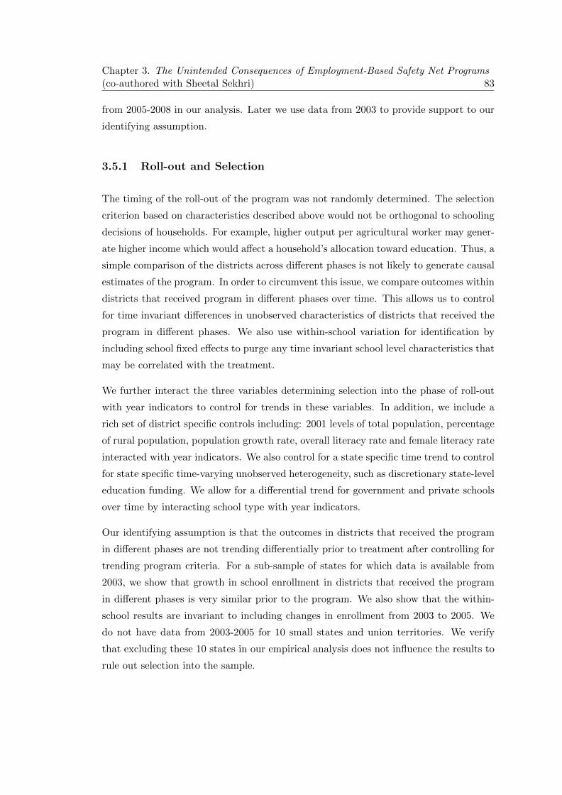
Chapter 3. The Unintended Consequences of Employment-Based Safety Net Programs(co-authored with Sheetal Sekhri) 83
from 2005-2008 in our analysis. Later we use data from 2003 to provide support to our
identifying assumption.
3.5.1 Roll-out and Selection
The timing of the roll-out of the program was not randomly determined. The selection
criterion based on characteristics described above would not be orthogonal to schooling
decisions of households. For example, higher output per agricultural worker may gener-
ate higher income which would affect a household’s allocation toward education. Thus, a
simple comparison of the districts across different phases is not likely to generate causal
estimates of the program. In order to circumvent this issue, we compare outcomes within
districts that received program in different phases over time. This allows us to control
for time invariant differences in unobserved characteristics of districts that received the
program in different phases. We also use within-school variation for identification by
including school fixed effects to purge any time invariant school level characteristics that
may be correlated with the treatment.
We further interact the three variables determining selection into the phase of roll-out
with year indicators to control for trends in these variables. In addition, we include a
rich set of district specific controls including: 2001 levels of total population, percentage
of rural population, population growth rate, overall literacy rate and female literacy rate
interacted with year indicators. We also control for a state specific time trend to control
for state specific time-varying unobserved heterogeneity, such as discretionary state-level
education funding. We allow for a differential trend for government and private schools
over time by interacting school type with year indicators.
Our identifying assumption is that the outcomes in districts that received the program
in different phases are not trending differentially prior to treatment after controlling for
trending program criteria. For a sub-sample of states for which data is available from
2003, we show that growth in school enrollment in districts that received the program
in different phases is very similar prior to the program. We also show that the within-
school results are invariant to including changes in enrollment from 2003 to 2005. We
do not have data from 2003-2005 for 10 small states and union territories. We verify
that excluding these 10 states in our empirical analysis does not influence the results to
rule out selection into the sample.

Chapter 3. The Unintended Consequences of Employment-Based Safety Net Programs(co-authored with Sheetal Sekhri) 84
3.5.2 Estimation Procedure
We use school level data from 1.13 million schools from 2005 to 2008 to test our hy-
potheses. Our empirical specification is as follows:
Yidst = α0 +α1MGNREGAdt+α2 Xidst+α3 Zds∗Tt+α4 States∗trend+Tt+Iids+εidst
(3.1)
where Yidst is the outcome variable for school i in district d in state s in year t.
MGNREGAdt is an indicator that takes value 1 if district d in state s has started
the MGNREGA program in year t, and 0 otherwise; Xidst is a vector of school level
controls including different kinds of incentives received by the students, and the charac-
teristics of the teachers and infrastructure of the school i in district d in state s in year t;
Zds is a vector of district-level controls for demographic characteristics, and is interacted
with year indicators to control for trends; States is a vector of state indicators, and is
interacted with time trends to control for state-specific trends; Tt and Iids are year- and
school-fixed effects,respectively, and εidst is the idiosyncratic error term. We drop the
MGNREGA phase indicators due to multi-collinearity in our school fixed effects model.
We cluster errors at the district level to account for arbitrary correlation over time.
In order to examine the school choices by school type, we interact the introduction of
MGNREGA with the type of school. The empirical model is as follows:
Yidst = β0 + β1MGNREGAdt + β2 Pids ∗MGNREGAdt + β3 Gids ∗MGNREGAdt
+β4 Xidst + β5 Zds ∗ Tt + β6 States ∗ trend+ β7 Schooltypei ∗ Tt + Tt + Iids + εidst
where Yidst is the outcome variable for school i in district d in state s in year t. Pids
is an indicator equal to 1 for private schools and 0 otherwise and Gids is an indicator
which takes value 1 for government schools and 0 otherwise. The omitted category is
others. We include the the interaction of the MGNREGA policy indicator with each of
these type indicators to examine whether enrollment differs by school type. Schooltypei
are indicators for government and private schools, and these are interacted with year
indicators to control for differential trends in different types of schools. Note that once
we include the school fixed effects, indicators for school type (private and government)
are not included as these are time invariant properties of schools. As before, we also
drop the phase indicators due to multi-collinearity in the school fixed effects model.
The outcomes we examine are: enrollment, pass rate, pass rate conditional on taking
the exams, pass rate of those who pass with more than 60 percent marks.

Chapter 3. The Unintended Consequences of Employment-Based Safety Net Programs(co-authored with Sheetal Sekhri) 85
3.6 Results
3.6.1 Overall Enrollment
We test the implications of the the conceptual framework we presented in Section 3.3.
First, in order to evaluate the effect of MGNREGA on equilibrium overall enrollment,
we estimate equation 1 and present the results in Table 3.4. Column (i) presents the
basic difference-in-difference specification with school and year fixed effects. This result
is robust to controlling for state specific time trends as reported in Column (ii), which
may capture state spending priorities. Both specifications control for district level con-
trols that influenced the roll-out priorities. We control for the Scheduled Castes and
Tribes population as per Census of India 1991, agricultural wage in 1996-97, and out-
put per agricultural worker in 1990-93, interacted with time indicators to account for
the backward district status that influenced selection into the program. In addition,
we also control for the districts level total population, percentage of urban population,
population growth rate, overall literacy rate, and women’s literacy rate. The school-
level controls include any attendance scholarships being offered at the time, uniform,
books, stationery and other such subsidies offered to girls, the number of classrooms,
the number of classrooms in good condition, availability of common toilets, girls toilets,
drinking water facilities, electrification status, number of male teachers, and number of
female teachers.
The coefficient in Column (i) is -2.23 and is statistically significant at the 5 percent level.
Overall, enrollment in this period is increasing and thus this coefficient indicates that
introduction of MGNREGA results in a smaller increase in within school enrollment in
treated districts across the years in the sample. Hence, implementation of MGNREGA
results in relative slower growth in enrollment, with 2 fewer children enrolled per school
in the treated districts.
When split by primary and upper primary grades, it is clear that this effect is driven
by primary classes where the magnitude is 2.23 (Columns (iii) and (iv)). This implies
that young children either substitute for adults in home production or are being taken
to work sites due to unavailability of suitable after school child care. We do not find
any change in the enrollment of children in upper-primary classes. Since these children
are already past elementary school (which is free in case of government schools), it is

Chapter 3. The Unintended Consequences of Employment-Based Safety Net Programs(co-authored with Sheetal Sekhri) 86
possible that households do not want to withdraw these children from schools as they
have invested in their schooling substantially. 17
3.6.2 Effects on Enrollment by Type of Schools
In order to examine if the type of school that children attend is affected due to an
increase in the income of the parents, we evaluate equation 2 and report the results in
Table 3.5. In Table 3.5, we show the interaction of the MGNREGA implementation
policy dummy interacted with government school indicator and private school indicator.
The excluded category is ‘other types’ schools. Columns (i), (iii), and (v) repeat the
results of the estimation of equation 1 for overall enrollment, primary enrollment and
upper-primary enrollment with additional controls for school type by year fixed effects.
Overall enrollment in government schools is not influenced, whereas there is a signifi-
cant reduction in enrollment for private schools (Column (ii)). The coefficient on the
interaction term with the private school indicator is significant at the 5 percent level.
This result is driven by primary schools (Columns (iii) - (vi)). Since 66 percent schools
in the data are government schools and only 13 percent are private schools, the decrease
in enrollment per private school is much larger in magnitude. The effect of the program
on overall enrollment is small in magnitude. Using the average number of government,
private and other schools per district in the sample period, our results indicate that
9,824 children per district are not attending school due to the program.18
3.6.3 Schooling Outcomes
We examine the effect on schooling outcomes to determine if the program has intensive
margin effects. Data reports passing outcomes and passing with more than 60 percent for
grade 5 and grade 7. In Table 3.6, we show that the passing rate in government schools
falls by 1.8 percent for grade 7 students (Columns (ii) and (iv)) with the coefficient
significant at the 10 percent significance level , whereas there is no effect on grade 5
(Columns (i) and (iii)). Passing with more than 60 percent marks undergoes a significant
change. For grade 7 students, both in private and government schools, there is a decline
17 However, it is also possible that households who are employed in MGNREGA sites are younger anddo not have children beyond the primary grades. In our subsequent analysis, we do observe heterogenouseffects on children in upper primary schools as well. Hence we do not think that participating household’sdemographic composition is driving these results.
18In results not shown, we do not find any differences in effects for girls versus boys.

Chapter 3. The Unintended Consequences of Employment-Based Safety Net Programs(co-authored with Sheetal Sekhri) 87
in pass rate with more than 60 percent marks. This effect is almost twice as large for
government schools than the private schools and the difference is statistically significant
(Columns (vi) and (viii)).
Thus, younger children seem to be effected on the extensive margin and their enrollment
falls. Older children, on the other hand, continue in school but their schooling outcomes
deteriorate.
3.6.4 Mechanisms
Several qualitative findings corroborate our quantitative finding that the program in-
duces primary school aged children to withdraw from school.19 In order to shed direct
light on the mechanism, we examine the employment outcomes of children in our DID
framework. The data on child labor come from the National Sample Survey Organiza-
tion (NSSO) employment and unemployment surveys (rounds 2004-05 to 2008-09) and
we employ earlier rounds to carry out a falsification check. The data asks individuals
to identify their principal occupation in the last month. We examine two outcome vari-
ables: Child reports working (employed, self employed or unpaid family labor) and child
reports doing chores (housework or free collection of goods). We restrict our sample to
206,321 non-disabled children aged between 5 and 15 from the two rounds and look at
their reported principle activities. The indicator for ‘working’ equals to 1 if a child’s
reported principle activity is working in the household enterprises (paid or unpaid), as
wage employee, or in other types of work, and 0 otherwise. The indicator for doing
chores is 1 if a child’s reported principle activity is attending to domestic duty or doing
any other housework, and 0 otherwise. 20
The empirical model is as follows:
Lidst = γ0 + γ1 PhaseI ∗Post+ γ2 PhaseII ∗Post+ γ3 Zds ∗ Tt + Tt + Ids + εidst (3.2)
19The field work conducted by Centre for Social Protection (Sudarshan, 2011) indicates that a majorityof women who work in MGNREGA projects take their primary school aged children to work sites orleave them at home to provide child care for younger siblings. The study conducted semi-structuredinterviews of the women on NREGA sites in various districts. One woman reported “Nobody is there tolook after the child. Women have to take care of their own children. Some women do come with a smallbaby but they bring along an older son or daughter to take care of the infant while the woman carriesout her work.” The field investigators reported that older children seemed to be 10 to 12 years old.When the interviewer asked if these children go to school, one woman said, “Madam jo site par jayegawoh school kaise ja sakta hai?” (If a child has to go to the site how can she go to school?). At anotherplace, the response was, “Women do not come with their children but leave their children at home withother siblings who look after them.” Other field studies have reported similar findings (Bhatty, 2006).
20Other alternatives for principle activity include attending educational institution, seeking jobs, ren-tiers, pensioners, remittance recipients, and others.

Chapter 3. The Unintended Consequences of Employment-Based Safety Net Programs(co-authored with Sheetal Sekhri) 88
where Lidst is the reported labor outcome of child i in district d in state s at time
t. PhaseI and PhaseII are the indicators for the respective phases; Zds is a vector
of district-level controls for demographic characteristics, and is interacted with year
indicators to control for trends; Tt and Ids are year- and district-fixed effects, respectively,
and εidst is the idiosyncratic error term.
After the program, there is a 1.33 percent increase in the likelihood of child reporting
working in Phase-I districts relative to Phase-III districts (Column (i) of Table 3.7).
This is significant at the 5 percent significance level. In Phase-II districts, this effect
is 1.17 percent increase marginally significant at the 10 percent significance level. We
cannot reject the equality of these two coefficients. In column (ii), we do not find any
changes in reporting doing chores. Hence, these effects are driven by increase in labor
substitution. Our findings indicate that child labor supply increases in response to the
program.
3.7 Robustness Checks and Sensitivity Analysis
Our identifying assumption is that there are no pre-trends in enrollment in districts
belonging to different phases prior to MGNREGA’s implementation. DISE data is not
available for all states prior to 2005, although major states are covered since 2003. We
use data from 2003 to 2005 to check if there are differential pre-trends in enrollment by
phases of MGNREGA roll-out. Since we are using a sub-sample of states from our main
sample to conduct this test, we first show that this sub-sample is not selected in any
way that can confound our results. There are 10 states or Union Territories for which
data is not available in years subsequent to 2003 but prior to 2005 and are thus used
in the empirical analysis in the paper.21 We exclude these states from our sample and
replicate the analysis from Table 3.4 and Table 3.5 for only the states for which DISE
data is available since 2003. The results from this exercise are reported in Tables 3.10
and 3.11 and are remarkably similar to those reported in Tables 3.4 and 3.5. This test
assures that selection into the sample does not confound our results.
Given that our main results are no different if we exclude or include these states, we
proceed to show that for the sample for which we have the pre-program data, the pre-
trends in enrollment are similar. Phase-III districts are better in levels. But the growth
21 These states or Union territories are: Jammu and Kashmir, Haryana, Arunachal Pradesh, Manipur,Daman and Diu, Dadra and Nagar Haveli, Goa, Lakshadweep, Pondicherry, and Andaman and NicobarIslands.

Chapter 3. The Unintended Consequences of Employment-Based Safety Net Programs(co-authored with Sheetal Sekhri) 89
rate in enrollment is similar. Figures 3.2 and 3.3 show that between 2003 and 2005, the
growth in enrollment and number of schools looks similar across districts in different
phases. 22 In Table 3.8, we control for district-specific changes in enrollment from 2003
to 2005 (pre-treatment years) and allow this to vary over time by interacting with year
indicators for the states for which we have pre-program data.23 The overall effect on
enrollment and enrollment by primary and upper primary are similar to those reported
in Table 3.5 and Table 3.11. These two tests together show that pre-trends in enrollment
are not biasing our results.
We also conduct an event study analysis to examine the timing of the effects for the states
that we have the data from 2003 onwards. We run a year-by year difference-in-difference
model comparing early versus late MGNREGA districts and plot the coefficients in
Figure 3.4. We observe a large decline in enrollment in 2006, the year MGNREGA was
introduced and subsequently enrollment in early phase districts continues to be lower
relative to the pre-program years. This further substantiates our study design.24
In Table 3.9, we run a placebo falsification exercise to test if the increase in likelihood
of employment post treatment in Phase-I and Phase-II districts relative to Phase-III
districts is due to a pre-trend. We use 1998-99 and 2004-05 years and run the same
equation (3) DID empirical specifications as Table 3.7. The results from this placebo
test reveal insignificant effects on child employment in in Phase-I and Phase-II districts
unlike the results reported in Table 3.7.
3.8 Alternative Channels
3.8.1 Other Programs
The Government of India introduced two programs in the early 2000s to promote direct
enrollment in schools. The first program, the Sarva Shiksha Abhiyan (SSA, was intended
to provide universal access to elementary education for children between 6-14 years.
SSA directly aimed to increase enrollment, retention, and the quality of education in
22Limited data for a few states is also available for 2001 and 2002 but the coverage is not as expansive.Since data for many states and many variables is not available, we do not use these years.
23We lose 0.7 percent of our sample schools as new districts were carved in 2004 and we are unable touse their pre-trend data.
24Note that for 2003 and 2004, we do not have several school level control variables in the data.Specifically, we do not have data on teacher characteristics and school infrastructure variables. Thus,the regression analysis in this event study excludes these variables. Also, we get the same patterns if weuse 2002 as baseline year instead of 2003.

Chapter 3. The Unintended Consequences of Employment-Based Safety Net Programs(co-authored with Sheetal Sekhri) 90
elementary schools by infrastructure provision and scholarships for marginalized social
groups. The provisions also aimed to eliminate gender differences. This program was
started in 2001, much earlier than the launch of MGNREGA. Although this program
targeted educationally backward blocks, these did not coincide with the districts in
a particular phase of MGNREGA. Another government of India program, the Midday
meal scheme, was also intended to increase school enrollment. This program was in effect
prior to 2000 and following a 2001 Supreme Court directive, states increased outlays for
this program. Thus the intensity of coverage increased sharply in many states following
this directive. This program was in place for several years before the introduction of
MGNREGA. In addition, many states increased provision of midday meals at the same
time. Therefore, the timing did not coincide with MGNREGA’s phased roll-out and we
do not think that our results are confounded by these programs.
3.8.2 Growth and Demand for Private Schools
One concern might be that the increase in private schools driven by growth in the private
school market, independent of the program, affects our results. For example, economic
growth may increase the demand for private schooling. During this time, the Indian
economy was growing very rapidly and the demand for schooling maybe increasing as
well. We see significant declines in the enrollment in the private schools. Hence, an
increase in number of schools cannot be causing this decline. Nevertheless, we address
this concern. Any global economic shocks are captured by the time fixed effects. In
addition, the estimates are robust to including state specific trends, and school type
by year fixed effects. Therefore, different trajectories of growth across states is not
generating our results and it is unlikely that growth driven demand for private schools
drives our results. In addition, we examine trends in expansion of schools visually.
Figure 3.5 shows phase wise trends in expansion of schools. Panel A shows trends for
government schools and Panel B shows the trends for private schools. Regardless of the
school type, these trends are very similar across early and late MGNREGA districts.
Thus, an independent increase in demand for private schools is unlikely to be driving
our results.
3.8.3 Migration and Population Changes
Anecdotal evidence suggests that MGNREGA reduced out-migration from poor districts
to richer ones. To the extent that this does not change the composition of the districts

Chapter 3. The Unintended Consequences of Employment-Based Safety Net Programs(co-authored with Sheetal Sekhri) 91
before and after the program, this should not be a concern for our analysis. One concern
is that we show changes in enrollment but not enrollment rate. We address this using the
baseline district population from the Census of India 2001 and interacting it with time
indicators to control flexibly for trends in population. If MGNREGA attracts migrants
into districts, then the results could be driven by changes in population. Across district
migration in India is very low (Topolova, 2010). Land markets are thin so households
do not tend to permanently migrate, at least in the short run. Finally, if migration were
responsible for the changes in enrollment, then we would expect similar sized effects
for primary and upper primary grades and individual classes within these grades. As
shown in Tables 3.4 and 3.5 and Tables 3.10 and 3.11, the size of the effect is much
larger in primary school with no effect discerned in upper primary school. It seems
implausible that households with children only in specific age groups would migrate into
the MGNREGA districts to find work, especially since the early phase districts were
poorer and have worse infrastructure. It is less likely that our results are confounded by
the changes in population due to massive in-migration.25
3.9 Caveats
We do not have age specific population data. Ideally, we should normalize our results
by this age specific population data. But since we do not have this data, we control for
trends in district specific total population. In addition, as argued above, any changes
in population growth cannot explain all our findings.26 But our results should be inter-
preted in light of this limitation.
3.10 Conclusion
We use the phased roll-out of MGNREGA to estimate the impact of safety net programs
such as employment guarantee schemes on schooling outcomes of children. Our findings
have important policy implications. We find that the enrollment in primary grades in-
creases less due to the program. Our results show that the program induces younger
25 Also, anecdotal evidence suggests that beneficiaries use the employment guarantee in summermonths. One concern might be that schools are already closed for vacation. However, schools in Indiagenerally close for only around 40 days and the timing varies spatially ranging from mid-May to endof June in North to mid-June to end-July in the South. Also, Imbert and Papp (2015) show that theprogram impacts rural wages in a general equilibrium framework. Given that there is an incentive tosubstitute for adult labor year round.
26 We also get similar results using log specifications.

Chapter 3. The Unintended Consequences of Employment-Based Safety Net Programs(co-authored with Sheetal Sekhri) 92
children to substitute for adults in employment outside the house. Among those already
enrolled, school pass rate with more than 60 percent marks declines for grade 7 but not
grade 5 students. Hence, these older children are influenced on the intensive margin.
Unless state or market institutions increase support to offset this perverse effect, such
safety programs are not likely to improve the schooling outcomes of children. Social wel-
fare programs are increasingly becoming reliant on micro-ordeals like work for benefits.
Our study shows that these programs can have unintended consequences for children of
the beneficiaries, which are not accounted for in welfare calculations.

Chapter 3. The Unintended Consequences of Employment-Based Safety Net Programs(co-authored with Sheetal Sekhri) 93
Bibliography
Afridi, F. , A.p Mukhopadhyay, and S. Sahoo (2012), “ Female Labour Force Partic-
ipation and Child Education in India: The Effect of the National Rural Employment
Guarantee Scheme”, IZA Discussion Paper No. 6593.
Alatas, V., A. Banerjee, R. Hanna, B. Olken, R. Purnamasari, and M. Wai-poi (2013),
“Ordeal Mechanisms In Targeting: Theory And Evidence From A Field Experiment In
Indonesia”, NBER working paper 19127.
Angelucci, M. and G. Giorgi (2009), “ Indirect Effects of an Aid Program: How do Cash
Injections Affect Ineligibles’ Consumption?”, American Economic Review, Vol. 99 (1),
pp.486-508.
Ardington, C., A. Case, and V. Hosegood (2009), “ Labor Supply Responses to Large So-
cial Transfers: Longitudinal Evidence from South Africa,” American Economic Journal:
Applied Economics, Vol. 1 (1), pp. 22-48.
Azam, M. (2012),“ The Impact of Indian Job Guarantee Scheme on Labor Market
Outcomes: Evidence from a Natural Experiment,” IZA Discussion Paper.
Basu, A. K. (2011), “ Impact of Rural Employment Guarantee Schemes on Seasonal
Labor Markets: Optimum Compensation and Workers’ Welfare” IZA Discussion Paper
No. 5701.
Basu, A. K., N. H. Chau, and R. Kanbur (2009), “ A Theory of Employment Guarantees:
Contestability Credibility and Distributional Concerns,” Journal of Public economics,
Vol. 93 (4), pp. 482-497.
Basu, K. (1999), “Child Labor: Cause, Consequence, and Cure, with Remarks on Inter-
national Labor Standards,” Journal of Economic Literature, vol. 37(3), pp. 1083-1119.
Basu, K. and P. H. Van(1998), “The Economics of Child Labor”, American Economic
Review, vol. 88, pp. 412-27.
Berg, E., S. Bhattacharyya, R. Durgam, and M. Ramachandra (2012), “ Can Rural
Public Works Affect Agricultural Wages? Evidence from India”, CSAE Working Paper
2012-05.
Bernstein, Barton J. (1968), “ The New Deal: The Conservative Achievements of Lib-
eral Reform” Towards a New Past: Dissenting Essays in American History, edited by
Bernstein, Barton J., New York: Pantheon Books.

Chapter 3. The Unintended Consequences of Employment-Based Safety Net Programs(co-authored with Sheetal Sekhri) 94
Besley, T. and S. Coate (1992), “ Workfare versus Welfare: Incentive Arguments for
Work Requirements in Poverty-Alleviation Programs,” American Economic Review, Vol.
82 (1), 249-261.
Bhatty, K. (2006) “Employment guarantee and child rights”, Economic and Political
Weekly, pp. 1965-1967.
Blaug, M. (1963),“ The Myth of the Old Poor Law and the Making of the New,” Journal
of Economic History Vol. 23, 151 - 184.
Blaug, M. (1964), “ The Poor Law Report Re-examined,” Journal of Economic History
Vol. 24, 229 - 245.
Datt, G. and M. Ravallion (1994), “ Transfer Benefits from Public-Works Employment:
Evidence for Rural India,” The Economic Journal,Vol. 104 (427), 1346-1369.
Desia, S., Dubey,A., Vanneman,R. and R. Banerji (2008), “Private Schooling in India:
A New Educational Landscape”, India Human Development Survey Working Paper 11.
Dreze, J. and A. Goyal (2003), “ The future of mid-day meals, Economic and Political
Weekly November 1, 4673-4683.
Duflo, E. (2003), “Grandmothers and Granddaughters: Old-Age Pensions and Intra-
household Allocation in South Africa”, World Bank Economic Review, Vol. 17, pp.
1-25.
Dupas, P., V. Hoffmann, M. Kremer, and A. Zwane (2013), “Micro-ordeals and preven-
tive health products: Evidence on short-term take-up and habit formation”.
Edmonds, E. (2006), “Child Labor and Schooling Responses to Anticipated Income in
South Africa,” Journal of Development Economics, vol. 81(2), pp. 386-414.
Edmonds, E. and N. Pavnick (2004), “The Effect of Trade Liberalization on Child La-
bor,” Journal of International Economics.
Edmonds,E. (2005), “Does Child Labor Decline with Improving Economic Status?,”
Journal of Human Resources,vol. 40(1).
Imbert, C. and J. Papp (2015), “Labor market effects of social programs: Evidence from
Indias Employment Guarantee” American Economic Journal:Applied Economics, Vol.
7(2), pp. 233-263

Chapter 3. The Unintended Consequences of Employment-Based Safety Net Programs(co-authored with Sheetal Sekhri) 95
Institute of Applied Manpower Research (2009), “ All-India Report on Evaluation of
NREGA: A Survey of Twenty Districts”.
Kremer, M. and K. Muralidharan (2007) ,“ Public and Private Schools in Rural India”,
Harvard University unpublished manuscript.
Jacoby, H. and E. Skoufias (1997), “Risk, Financial Markets, and Human Capital in a
Developing Country”, Review of Economic Studies, vol. 64, pp. 311-335.
Jayachandran, S., J. Cunha, and G. D. Giorgi (2010), “ The Price Effect of Cash Versus
In-Kind Transfers”, CEPR Development Economics Workshop Working Paper.
Jensen, R. (2010), “The (Perceived) Returns to Education and the Demand for School-
ing,” Quarterly Journal of Economics, Vol. 125(2), pp. 515-548.
Kesselman, Jonathan R. (1978), “ Work relief programs in the Great Depression” Cre-
ating Jobs: Public Employment Programs and Wage Subsidies, edited by Palmer, J.L.,
Washington, D.C.: Brookings Institution.
Khera, R. (Ed.) (2011). The Battle for Employment Guarantee. Oxford University
Press.
Ministry of Rural Development (2008a), “Annual Report (2007-2008)”, Government of
India.
Ministry of Rural Development (2008b), “The National Rural Employment Guarantee
Act 2005 (NREGA): Operational Guidlines 2008”, Government of India.
Mukherjee, D. and U. B. Sinha (2013), “ Understanding NREGA: A Simple Theory and
Some Facts” Human Capital and Development: The Indian Experience, Ch 7, 103 - 128.
Murgai, R. and M. Ravallion (2005), “ Employment Guarantee in Rural India: What
Would It Cost and How Much Would It Reduce Poverty?” Economic and Political
Weekly, Vol.40 (31), 3450-3455.
Nichols, A. and R. Zeckhauser (1982), “Targeting Transfers through Restrictions on
Recipients,” American Economic Review, Papers and Proceedings, Vol. 72, pp. 372-7.
Niehaus, P. and S. Sukhtankar (2009), “ Corruption Dynamics: The Golden Goose
Effect”, BREAD Working Paper 223.
Psacharopoulos, G. (1997), “Child Labor versus Educational Attainment: Some Evi-
dence from Latin America”, Journal of Population Economics, vol. 10.

Chapter 3. The Unintended Consequences of Employment-Based Safety Net Programs(co-authored with Sheetal Sekhri) 96
Planning Commision (2003), “Identification of Districts for Wage and Self employment
programmes”.
Qian, Nancy (2008), “Missing Women and the Price of Tea in China: The Effect of
Sex-Specific Income on Sex Imbalance”, The Quarterly Journal of Economics, Vol. 123
(3).
Rogers, C. and K. Swinnerton, K. (2004), “Does Child Labor Decrease when Parental
Incomes Rise”, Journal of Political Economy, vol. 112.
Rosenzweig, M. and R. Evenson (1977), “Fertility, Schooling and the Economic Contri-
bution of Children in Rural India: An Econometric Analysis”, Econometrica, vol. 45,
1065-1079.
Ravi, S. and M. Engler (2009), “ Workfare in Low Income Countries: An Effective Way
to Fight Poverty? The Case of NREGS in India” Working paper.
Ravallion, M. (1991), “Reaching the Rural Poor Through Public Employment: Argu-
ments, Evidence, and Lessons from South Asia,” World Bank Research Observer Vol.
6(2), pp. 153175.
Ray, R. (2000), “Child Labor, Child Schooling and Their Interaction with Adult Labor
: Empirical Evidence for Peru and Pakistan”, World Bank Economic Review, vol. 14.
Schultz, T. P. (2004), “School Subsidies for the Poor: Evaluating the Mexican Progresa
Poverty Program”, Journal of Development Economics, vol. 74.
Shastry, G. (2012), “Human Capital Response to Globalization: Education and Infor-
mation Technology in India, ” Journal of Human Resources, Vol. 47(2), pp. 287-330.
Skoufias, E. (1993) , “Labor Market oppurtunities and Intrafamily time allocation in
Rural households in South Asia, ” Journal of Development Economics, Vol. 40(2), pp.
277-310.
Skoufias, E. and Parker, S. (2003), “The Impact of Progressa on Child Work and School-
ing” in P.F. Orazem, G. Sedlacek and Z. Tzannatos (eds.; forthcoming) ’Child Labor
and Education in Latin America’. Washington DC: InterAmerican Development Bank
and World Bank.
Sudarshan, R. (2011), “India’s National Rural Employment Guarantee Act: women’s
participation and impacts in Himachal Pradesh, Kerala and Rajasthan” , CSP Research
Report 06.

Chapter 3. The Unintended Consequences of Employment-Based Safety Net Programs(co-authored with Sheetal Sekhri) 97
Sharma, A. (2009),“ NCAER-PIF Study on Evaluating Performance of National Rural
Employment Guarantee Act,” National Council of Applied Economic Research.
Thomas, D. (1994), “Like Father Like Son; Like Mother Like Daughter: Parental Re-
sources and Child Height”, The Journal of Human Resources, Vol. 29, pp. 950-988.
Topalova, P. (2010), “ Factor Immobility and Regional Impacts of Trade Liberalization:
Evidence on Poverty and Inequality from India, American Economic Journal: Applied
Economics, Vol. 2 (4), pp. 1-41.

Chapter 3. The Unintended Consequences of Employment-Based Safety Net Programs(co-authored with Sheetal Sekhri) 98
Figure 3.1: Districts in Different Phases of NREGA
LegendCity DistrictsPhase IPhase IIPhase III

Chapter 3. The Unintended Consequences of Employment-Based Safety Net Programs(co-authored with Sheetal Sekhri) 99
Figure 3.2: Total Enrollment by Phases
Figure 3.3: Total Number of Schools by Phases

Chapter 3. The Unintended Consequences of Employment-Based Safety Net Programs(co-authored with Sheetal Sekhri) 100
Figure 3.4: Year Wise Impact
Figure 4: The figure plots year by year DID coefficients relative to baseline year 2003. NREGA was introduced in February, 2006. We observe a significant relative decline in enrollment in 2006 in early
NREGA districts relative to later ones. Subsequently, the enrollment is lower compared to pre‐program
years.
‐10
‐9
‐8
‐7
‐6
‐5
‐4
‐3
2004 2005 2006 2007 2008
Figure 4: Year Wise Impact
DID Coefficients, Phase I and II relative to Phase III
Note: The figure plots year by year DID coefficients relative to baseline year 2003. NREGA wasintroduced in February, 2006. We observe a significant relative decline in enrollment in 2006 in earlyNREGA districts relative to later ones. Subsequently, the enrollment is lower compared to pre-programyears.

Chapter 3. The Unintended Consequences of Employment-Based Safety Net Programs(co-authored with Sheetal Sekhri) 101
Figure 3.5: Phase Wise Expansion in Different Types of Schools
Figure 5: Phase Wise Expansion in Different Types of Schools
100000
150000
200000
250000
300000
2005 2006 2007 2008
Number of Government Schools by NREGA Phases
Phase 1 Phase 2 Phase 3
0
10000
20000
30000
40000
50000
60000
70000
80000
2005 2006 2007 2008
Number of Private Schools by NREGA Phases
Phase 1 Phase 2 Phase 3

Chapter 3. The Unintended Consequences of Employment-Based Safety Net Programs(co-authored with Sheetal Sekhri) 102
Table3.1:
Su
mm
ary
Sta
tist
ics
Ou
tcom
eva
riab
les
(All
ph
ase
s,all
years
)T
able
1: S
umm
ary
Stat
istic
s Out
com
e va
riab
les (
All
phas
es, a
ll ye
ars)
Obs
Mea
nSt
d. d
ev.
Min
Max
Tota
l3,
583,
317
220.
2221
5.20
116
155
Prim
ary
Cla
sses
3,05
3,18
021
4.50
194.
991
1614
5
Upp
er-p
rimar
y C
lass
es1,
113,
283
108.
7311
2.48
135
17
Gov
ernm
ent S
choo
ls2,
366,
670
222.
7121
1.16
116
155
Priv
ate
Scho
ols
471,
220
286.
8627
9.26
113
841
Oth
er S
choo
ls74
5,42
717
0.39
162.
481
8040
Gra
de 5
2,67
3,49
20.
900.
190
1
Gra
de 7
898,
816
0.87
0.21
01
Gra
de 5
2,74
4,76
30.
960.
140
1
Gra
de 7
921,
451
0.91
0.19
01
Gra
de 5
2,48
6,18
70.
430.
350
1
Gra
de 7
898,
816
0.39
0.33
01
Gra
de 5
2,54
6,73
70.
450.
350
1
Gra
de 7
921,
451
0.40
0.34
01
Enr
ollm
ent
Pass
ing
Rat
e co
nditi
onal
on
bei
ng e
nrol
lmen
t
Pass
ing
Rat
e co
nditi
onal
on
app
eari
ng in
the
exam
Pass
ing
60 c
ondi
tiona
l on
bein
g en
rollm
ent
Pass
ing
60 c
ondi
tiona
l on
appe
arin
g in
the
exam

Chapter 3. The Unintended Consequences of Employment-Based Safety Net Programs(co-authored with Sheetal Sekhri) 103
Table3.2:
Su
mm
ary
Sta
tist
ics-
Ou
tcom
eV
ari
ab
les
by
NR
EG
AP
hase
sT
able
2: S
umm
ary
Stat
istic
s- O
utco
me
Var
iabl
es b
y N
RE
GA
Pha
ses
Obs
Mea
nSt
d.O
bsM
ean
Std.
Obs
Mea
nSt
d.
Tota
l1,
427,
624
223.
7621
9.23
811,
704
230.
6421
7.60
1,34
3,98
920
9.82
207.
79Pr
imar
y1,
232,
837
219.
4019
8.22
690,
974
228.
0919
7.33
1,11
6,97
420
1.57
190.
42U
pper
-prim
ary
390,
848
113.
0111
7.09
231,
646
113.
0270
.65
490,
679
102.
1210
3.60
Gov
ernm
ent
1,00
6,79
523
3.43
224.
016
576,
487
242.
6022
1.81
578
3,38
819
4.43
181.
14Pr
ivat
e 13
3,14
629
3.19
281.
5994
,408
266.
9326
2.3
243,
666
291.
2228
4.06
Oth
ers
287,
683
158.
7214
4.31
140,
809
159.
3014
5.04
316,
935
185.
5418
2.38
Gra
de 5
996,
134
0.88
0.21
556,
877
0.90
0.19
928,
972
0.92
0.17
Gra
de 7
284,
491
0.86
0.23
170,
904
0.87
0.21
388,
192
0.88
0.20
Gra
de 5
1,02
3,75
80.
950.
1657
8,72
00.
960.
1494
7,59
10.
960.
12
Gra
de 7
290,
747
0.90
0.20
176,
551
0.91
0.19
397,
070
0.91
0.18
Gra
de 5
997,
423
0.38
0.34
558,
074
0.44
0.34
930,
690
0.49
0.35
Gra
de 7
285,
758
0.36
0.34
171,
654
0.36
0.32
389,
877
0.43
0.33
Gra
de 5
1,02
1,69
30.
400.
3557
8,10
30.
460.
3594
6,94
10.
510.
35
Gra
de 7
290,
652
0.37
0.35
176,
552
0.37
0.33
397,
220
0.44
0.33
Phas
e II
I
Pass
ing
Rat
e C
ondi
tiona
l on
Bei
ng
Enr
olle
d
Pass
ing
Rat
e C
ondi
tiona
l on
App
eari
ng in
Exa
ms
Phas
e I
Phas
e II
Pass
ing
60 C
ondi
tiona
l on
Bei
ng E
nrol
led
Enr
ollm
ent
Pass
ing
60 C
ondi
tiona
l on
App
eari
ng in
Exa
ms

Chapter 3. The Unintended Consequences of Employment-Based Safety Net Programs(co-authored with Sheetal Sekhri) 104
Table3.3:
Com
par
ison
of
Dis
tric
tL
evel
Ch
ara
cter
isti
csacr
oss
NR
EG
AP
hase
sT
able
3: C
ompa
riso
n of
Dis
tric
t Lev
el C
hara
cter
istic
s acr
oss N
RE
GA
Pha
ses
Yea
r of
M
easu
rem
ent
Mea
nSt
d D
ev.
Mea
nSt
d. D
ev.
Mea
nSt
d. D
ev.
Tot
al P
opul
atio
n (1
,000
peo
ple)
2001
1,83
11,
112
2,04
71,
429
1,99
21,
119
Popu
latio
n G
row
th r
ate
(%)
1991
-200
121
.13
6.96
21.1
88.
0320
.75
9.67
Ove
rall
Lite
racy
Rat
e (%
)20
0147
.16
10.4
552
.51
12.3
958
.23
10.3
2
Perc
enta
ge o
f Fem
ale
Popu
latio
n (%
)20
0148
.68
1.24
48.3
11.
2748
.04
1.98
Fem
ale
Lite
racy
rat
e (%
)20
0143
.55
12.5
549
.32
15.3
258
.46
14.1
7
Perc
enta
ge o
f Wor
king
Pop
ulat
ion
(%)
2001
42.2
56.
6540
.01
6.94
40.3
57.
12
Perc
enta
ge S
ched
uled
Cas
te19
9138
.42
20.7
431
.27
21.6
325
.76
20.8
7 a
nd S
ched
uled
Tri
be P
opul
atio
n (%
)
Agr
icul
tura
l wag
es (R
s/pe
rson
/Day
)19
96-9
732
.14
9.58
37.7
29.
8446
.44
18.4
8
Out
put p
er A
gric
ultu
ral W
orke
r19
90-1
993
5,19
63,
401
7,02
55,
212
11,8
689,
521
(Rs/
wor
ker)
Phas
e I
Phas
e II
Phas
e II
I

Chapter 3. The Unintended Consequences of Employment-Based Safety Net Programs(co-authored with Sheetal Sekhri) 105
Table3.4:
Th
eIm
pact
of
Intr
od
uct
ion
of
NR
EG
Aon
En
roll
men
t(2
005-0
8)
T
able
4: T
he Im
pact
of I
ntro
duct
ion
of N
RE
GA
on
Enr
ollm
ent (
2005
-08)
Dep
ende
nt V
aria
ble:
Tot
al E
nrol
lmen
t
Prim
ary
Upp
er P
rim
ary
(i)(ii
)(ii
i)(iv
)
-2.2
3**
-1.9
6**
-2.2
3**
-0.4
2(1
.02)
(0.9
5)(1
.04)
(0.5
6)
Yea
r Fix
ed E
ffec
tsY
esY
esY
esY
esSc
hool
Fix
ed E
ffec
tsY
esY
esY
esY
esD
istri
ct D
emog
raph
ics
Yes
Yes
Yes
Yes
Con
trols
for B
ackw
ardn
ess
Yes
Yes
Yes
Yes
Ince
ntiv
esY
esY
esY
esY
esSc
hool
Infr
ustru
ctur
eY
esY
esY
esY
esN
umbe
r of T
each
ers
Yes
Yes
Yes
Yes
Stat
e Ti
me
Tren
dN
oY
esY
esY
es
Obs
erva
tions
3,05
3,18
01,
113,
283
Num
ber
of S
choo
ls94
1,39
037
8,32
4N
otes
:*** p<
0.01
, ** p<
0.05
, * p<0.1
i) Sc
hool
Ince
ntiv
e pr
ogra
ms i
nclu
de te
xtbo
oks,
stat
iona
ry, u
nifo
rms,
atte
ndan
ce sc
hola
rshi
p, a
nd o
ther
ince
ntiv
es; t
each
er c
hara
cter
istic
sin
clud
e th
e nu
mbe
r of m
ale
and
fem
ale
teac
hers
; inf
rast
ruct
ure
incl
udes
the
num
ber o
f cla
ssro
oms,
clas
sroo
ms i
n go
od c
ondi
tion,
the
exis
tenc
e of
com
mon
toile
t, w
omen
's to
ilet,
elec
trici
ty, a
nd w
ater
faci
litie
s; a
nd d
istri
ct le
vel d
emog
raph
ic c
hara
cter
istc
s inc
lude
tota
l pop
ulat
ion,
per
cent
age
of u
rban
pop
ulat
ion,
pop
ulat
ion
grow
th ra
te, o
vera
ll lit
erac
y ra
te, a
nd w
omen
's lit
erac
y ra
te.
ii) E
ach
regr
essi
on c
ontro
ls fo
r yea
r fix
ed e
ffec
ts a
nd sc
hool
fixe
d ef
fect
s. In
add
ition
, we
also
con
trol f
or
Sche
dule
d ca
stes
and
trib
es p
opua
tion
a pe
r Cen
sus o
f Ind
ia 1
991,
agr
icul
tura
l wag
e in
199
6-97
, and
out
put p
er a
gric
ultu
ral w
orke
r in
1990
-93,
inte
ract
ed w
ith ti
me
indi
cato
rs to
acc
ount
for t
he b
ackw
ard
dist
rict s
tatu
s tha
t inf
luen
ced
sele
ctio
n in
to th
e pr
ogra
m.
iii) R
obus
t sta
ndar
d er
rors
clu
ster
ed a
t dis
trict
leve
l are
repo
rted
in p
aran
thes
es.
3,58
3,31
71,
106,
957
NR
EGA
Com
men
ced
Ove
rall
Enr
olm
ent

Chapter 3. The Unintended Consequences of Employment-Based Safety Net Programs(co-authored with Sheetal Sekhri) 106
Table3.5:
Het
erog
neo
us
Imp
act
of
the
Intr
od
uct
ion
of
NR
EG
Aon
En
roll
men
t(2
005-0
8)
Tab
le 5
: Het
erog
neou
s Im
pact
of t
he In
trod
uctio
n of
NR
EG
A o
n E
nrol
lmen
t (20
05-0
8)
Prim
ary
Enr
ollm
ent
(i)(ii
)(ii
i)(iv
)(v
)(v
i)
-1.9
5**
-1.4
4-2
.20*
*-1
.59
-0.4
30.
15(0
.96)
(1.2
6)(1
.04)
-1.2
4(0
.68)
-0.8
3
0.39
0.74
-1.0
7(1
.83)
(1.9
0)(1
.03)
-8.2
1**
-12.
49**
*-0
.38
(3.3
8)(4
.10)
(1.4
6)
Gvt
Sch
ool*
Yea
r Dum
mie
sN
oY
esN
oY
esN
oY
esPv
t Sch
ool*
Yea
r Dum
mie
sN
oY
esN
oY
esN
oY
esIn
cent
ives
Yes
Yes
Yes
Yes
Yes
Yes
Teac
her C
hara
cter
istic
s Y
esY
esY
esY
esY
esY
esSc
hool
Infr
ustru
ctur
eY
esY
esY
esY
esY
esY
esD
istri
ct D
emog
raph
ics
Yes
Yes
Yes
Yes
Yes
Yes
Con
trols
for B
ackw
ardn
ess
Yes
Yes
Yes
Yes
Yes
Yes
Yea
r Fix
ed E
ffec
tsY
esY
esY
esY
esY
esY
esSc
hool
Fix
ed E
ffec
tsY
esY
esY
esY
esY
esY
esSt
ate
Tim
e Tr
end
Yes
Yes
Yes
Yes
Yes
Yes
Obs
erva
tions
Num
ber o
f Sch
ools
i) Sc
hool
Ince
ntiv
e pr
ogra
ms i
nclu
de te
xtbo
oks,
stat
iona
ry, u
nifo
rms,
atte
ndan
ce sc
hola
rshi
p, a
nd o
ther
ince
ntiv
es; t
each
er c
hara
cter
istic
sin
clud
e th
e nu
mbe
r of m
ale
and
fem
ale
teac
hers
; inf
rast
ruct
ure
incl
udes
the
num
ber o
f cla
ssro
oms,
clas
sroo
ms i
n go
od c
ondi
tion,
the
exis
tenc
e of
com
mon
toile
t, w
omen
's to
ilet,
elec
trici
ty, a
nd w
ater
faci
litie
s; a
nd d
istri
ct le
vel d
emog
raph
ic c
hara
cter
istc
s inc
lude
tota
l pop
ulat
ion,
per
cent
age
of u
rban
pop
ulat
ion,
pop
ulat
ion
grow
th ra
te, o
vera
ll lit
erac
y ra
te, a
nd w
omen
's lit
erac
y ra
te.
ii) E
ach
regr
essi
on c
ontro
ls fo
r yea
r fix
ed e
ffec
ts, s
choo
l fix
ed e
ffec
ts a
nd st
ate-
spec
ific
time
trend
s. Ea
ch re
gres
sion
als
o in
clud
esin
dica
tors
for t
he ty
pe o
f sch
ool a
nd w
heth
er sc
hool
off
ers p
rimar
y cl
asse
s and
\or u
pper
prim
ary
clas
ses.
In a
dditi
on, w
e al
so c
ontro
l for
Sche
dule
d ca
ste
popu
atio
n a
per C
ensu
s of I
ndia
199
1, a
gric
ultu
ral w
age
in 1
996-
97, a
nd o
utpu
t per
agr
icul
tura
l wor
ker i
n 19
90-9
3,in
tera
cted
with
tim
e in
dica
tors
to a
ccou
nt fo
r the
bac
kwar
d di
stric
t sta
tus t
hat i
nflu
ence
d se
lect
ion
into
the
prog
ram
.iii
) Rob
ust s
tand
ard
erro
rs c
lust
ered
at d
istri
ct le
vel a
re re
porte
d in
par
anth
eses
.
Upp
er P
rim
ary
Enr
ollm
ent
***
p<0.
01, *
* p<
0.05
, * p
<0.1
NR
EGA
Com
men
ced
NR
EGA
Com
men
ced
*
Gov
ernm
ent S
choo
l
NR
EGA
Com
men
ced
*Pr
ivat
e Sc
hool
Tot
al E
nrol
lmen
t
3,58
3,31
71,
106,
957
1,11
3,28
337
8,32
43,
053,
180
941,
390

Chapter 3. The Unintended Consequences of Employment-Based Safety Net Programs(co-authored with Sheetal Sekhri) 107
Table3.6:
Th
eIm
pac
tof
the
Intr
od
uct
ion
of
NR
EG
Aon
Per
form
an
ceO
utc
om
es(2
005-0
8)
Tab
le 6
: The
Impa
ct o
f the
Intr
oduc
tion
of N
RE
GA
on
Perf
orm
ance
Out
com
es (2
005-
08)
Gra
de 5
Gra
de 7
Gra
de 5
Gra
de 7
Gra
de 5
Gra
de 7
Gra
de 5
Gra
de 7
(i)(ii
)(ii
i)(iv
)(v
)(v
i)(v
ii)(v
iii)
0.39
-0.3
40.
34-0
.06
0.42
3.52
**0.
363.
75**
(0.4
2)(0
.63)
(0.3
4)(0
.62)
(0.7
3)(1
.73)
(0.7
4)(1
.78)
-0.4
7-1
.84*
-0.4
3-1
.71*
-0.2
5-5
.98*
**-0
.28
-6.1
1***
(0.6
7)(1
.01)
(0.5
8)(0
.98)
(0.8
8)(1
.83)
(0.8
9)(1
.89)
-0.3
5-0
.54
-0.2
5-0
.43
0.85
-3.8
0**
0.85
-4.0
2**
(0.5
3)(0
.65)
(0.3
7)(0
.56)
(0.8
7)(1
.70)
(0.8
7)(1
.74)
Gvt
Sch
ool*
Yea
r Dum
mie
sY
esY
esY
esY
esY
esY
esY
esY
esPv
t Sch
ool*
Yea
r Dum
mie
sY
esY
esY
esY
esY
esY
esY
esY
esIn
cent
ives
Yes
Yes
Yes
Yes
Yes
Yes
Yes
Yes
Teac
her C
hara
cter
istic
s Y
esY
esY
esY
esY
esY
esY
esY
esSc
hool
Infr
ustru
ctur
eY
esY
esY
esY
esY
esY
esY
esY
esD
istri
ct D
emog
raph
ics
Yes
Yes
Yes
Yes
Yes
Yes
Yes
Yes
Con
trols
for B
ackw
ardn
ess
Yes
Yes
Yes
Yes
Yes
Yes
Yes
Yes
Yea
r Fix
ed E
ffec
tsY
esY
esY
esY
esY
esY
esY
esY
esSc
hool
Fix
ed E
ffec
tsY
esY
esY
esY
esY
esY
esY
esY
esSt
ate
Tim
e Tr
end
Yes
Yes
Yes
Yes
Yes
Yes
Yes
Yes
Obs
erva
tions
2,41
2,91
080
7,70
92,
398,
334
807,
994
2,47
1,12
282
5,39
32,
450,
877
826,
621
Num
ber o
f Sch
ools
834,
812
311,
403
833,
173
314,
233
839,
023
313,
675
836,
656
316,
481
i) Sc
hool
Ince
ntiv
e pr
ogra
ms i
nclu
de te
xtbo
oks,
stat
iona
ry, u
nifo
rms,
atte
ndan
ce sc
hola
rshi
p, a
nd o
ther
ince
ntiv
es; t
each
er c
hara
cter
istic
sin
clud
e th
e nu
mbe
r of m
ale
and
fem
ale
teac
hers
; inf
rast
ruct
ure
incl
udes
the
num
ber o
f cla
ssro
oms,
clas
sroo
ms i
n go
od c
ondi
tion,
the
exis
tenc
e of
com
mon
toile
t, w
omen
's to
ilet,
elec
trici
ty, a
nd w
ater
faci
litie
s; a
nd d
istri
ct le
vel d
emog
raph
ic c
hara
cter
istc
s inc
lude
tota
l pop
ulat
ion,
per
cent
age
of u
rban
pop
ulat
ion,
pop
ulat
ion
grow
th ra
te, o
vera
ll lit
erac
y ra
te, a
nd w
omen
's lit
erac
y ra
te.
ii) E
ach
regr
essi
on c
ontro
ls fo
r yea
r fix
ed e
ffec
ts, s
choo
l fix
ed e
ffec
ts a
nd st
ate-
spec
ific
time
trend
s. Ea
ch re
gres
sion
als
o in
clud
esin
dica
tors
for t
he ty
pe o
f sch
ool a
nd w
heth
er sc
hool
off
ers p
rimar
y cl
asse
s and
\or u
pper
prim
ary
clas
ses.
In a
dditi
on, w
e al
so c
ontro
l for
Sche
dule
d ca
ste
popu
atio
n a
per C
ensu
s of I
ndia
199
1, a
gric
ultu
ral w
age
in 1
996-
97, a
nd o
utpu
t per
agr
icul
tura
l wor
ker i
n 19
90-9
3,in
tera
cted
with
tim
e in
dica
tors
to a
ccou
nt fo
r the
bac
kwar
d di
stric
t sta
tus t
hat i
nflu
ence
d se
lect
ion
into
the
prog
ram
.iii
) Rob
ust s
tand
ard
erro
rs c
lust
ered
at d
istri
ct le
vel a
re re
porte
d in
par
anth
eses
.
Pass
60/
App
eari
ng a
t E
xam
Pass
60/
Enr
ollm
ent
Pass
/App
eari
ng a
t E
xam
***
p<0.
01, *
* p<
0.05
, * p
<0.1
NR
EGA
Com
men
ced
(uni
t: %
)
NR
EGA
Com
men
ced
*G
ov't
Scho
ol (u
nit:
%)
NR
EGA
Com
men
ced
*Priv
ate
Scho
ol (u
nit:
%)
Pass
/Enr
ollm
ent

Chapter 3. The Unintended Consequences of Employment-Based Safety Net Programs(co-authored with Sheetal Sekhri) 108
Table3.7:
Lin
ear
Pro
bab
ilit
yR
egre
ssio
nR
esu
lts
on
Ch
ild
Lab
or
(Age:
5-
15)
Tab
le 7
: Lin
ear
Prob
abili
ty R
egre
ssio
n on
Chi
ld L
abor
(Age
: 5 -
15)
Usi
ng N
SSO
Dat
a R
ound
61
(200
4-05
) and
Rou
nd 6
6 (2
008-
09)
Out
com
e V
aria
bles
Chi
ld re
porte
d w
orki
ng
(em
ploy
ed, s
elf-
empl
oyed
, or
unpa
id fa
mily
labo
r)
Chi
ld re
porte
d do
ing
chor
es
(hou
sew
ork
or fr
ee c
olle
ctio
n of
goo
ds)
(i)(ii
)
1.33
**0.
43(0
.634
)(0
.56)
1.17
*0.
36(0
.67)
(0.5
1)
Dis
trict
FE
and
Yea
r FE
Yes
Yes
Dis
trict
-leve
l Con
trols
Yes
Yes
Obs
erva
tions
206,
321
206,
321
# of
Dis
trict
s43
843
8**
* p<
0.01
, **
p<0.
05, *
p<0
.1i)
Each
regr
essi
on c
ontro
ls fo
r yea
r fix
ed e
ffec
ts a
nd d
istri
ct fi
xed
effe
cts.
Dis
trict
-leve
l con
trols
incl
ude
sche
dule
d ca
ste
popu
atio
n a
per C
ensu
s of I
ndia
199
1, a
gric
ultu
ral w
age
in 1
996-
97, a
nd o
utpu
t per
agr
icul
tura
l wor
ker
in 1
990-
93, i
nter
acte
d w
ith ti
me
indi
cato
rs to
acc
ount
for t
he b
ackw
ard
dist
rict s
tatu
s tha
t inf
luen
ced
sele
ctio
n in
to th
e pr
ogra
m.
ii) R
obus
t sta
ndar
d er
rors
clu
ster
ed a
t dis
trict
leve
l are
repo
rted
in p
aran
thes
es.
Phas
e 1*
Post
(Uni
t: %
)
Phas
e 2*
Post
(Uni
t: %
)

Chapter 3. The Unintended Consequences of Employment-Based Safety Net Programs(co-authored with Sheetal Sekhri) 109
Table3.8:
Th
eIm
pac
tof
the
Intr
od
uct
ion
of
NR
EG
Aon
En
roll
men
t(2
005-0
8)
Contr
oll
ing
Pre
-tre
nd
sfr
om
2003
to2005
Con
trolli
ng p
re-tr
ends
from
200
3 to
200
5, e
xclu
ding
stat
es fo
r whi
ch 2
003-
2005
dat
a is
una
vaila
ble.
Tab
le 6
: The
Impa
ct o
f the
Intr
oduc
tion
of N
RE
GA
on
Enr
ollm
ent (
2005
-08)
(i)(ii
)(ii
i)(iv
)(v
)(v
i)-1
.91*
*-1
.345
-2.1
5**
-1.5
49-0
.43
0.39
1(0
.97)
(1.3
00)
(1.0
6)(1
.304
)(0
.61)
(0.8
37)
0.31
40.
755
-1.4
08(1
.903
)(1
.975
)(1
.078
)-8
.183
**-1
2.43
***
-0.4
91(3
.387
)(4
.183
)(1
.466
)
Gvt
Sch
ool*
Yea
r Dum
mie
sN
oY
esN
oY
esN
oY
esPv
t Sch
ool*
Yea
r Dum
mie
sN
oY
esN
oY
esN
oY
esIn
cent
ives
Yes
Yes
Yes
Yes
Yes
Yes
Teac
her C
hara
cter
istic
s Y
esY
esY
esY
esY
esY
esSc
hool
Infr
ustru
ctur
eY
esY
esY
esY
esY
esY
esD
istri
ct D
emog
raph
ics
Yes
Yes
Yes
Yes
Yes
Yes
Con
trols
for B
ackw
ardn
ess
Yes
Yes
Yes
Yes
Yes
Yes
Con
trols
for P
re-tr
end
Yes
Yes
Yes
Yes
Yes
Yes
Yea
r an
d Sc
hool
Fix
ed E
ffec
Yes
Yes
Yes
Yes
Yes
Yes
Stat
e Ti
me
Tren
dY
esY
esY
esY
esY
esY
esO
bser
vatio
ns
i) Ex
clud
ed Ja
mm
u an
d K
ashm
ir, H
arya
na, A
runa
chal
Pra
desh
, Man
ipur
, Dam
an a
nd D
iu, D
adra
and
Nag
ar H
avel
i, G
oa,
Laks
hadw
eep,
Pon
dich
erry
, and
And
aman
and
Nic
obar
Isla
nds,
to fo
rm a
con
sist
ent p
anel
with
Fig
ures
1-6
.ii)
We
also
add
the
cont
rols
for d
istri
ct-le
vel p
re-tr
ends
, whi
ch in
clud
e th
e ch
ange
s fro
m 2
003-
04, a
nd 2
004-
05, i
nter
acte
d w
ith y
ear d
umm
ies.
iii) S
choo
l Inc
entiv
e pr
ogra
ms i
nclu
de te
xtbo
oks,
stat
iona
ry, u
nifo
rms,
atte
ndan
ce sc
hola
rshi
p, a
nd o
ther
ince
ntiv
es; t
each
er c
hara
cter
istic
sin
clud
e th
e nu
mbe
r of m
ale
and
fem
ale
teac
hers
; inf
rast
ruct
ure
incl
udes
the
num
ber o
f cla
ssro
oms,
clas
sroo
ms i
n go
od c
ondi
tion,
the
exis
tenc
e of
com
mon
toile
t, w
omen
's to
ilet,
elec
trici
ty, a
nd w
ater
faci
litie
s; a
nd d
istri
ct le
vel d
emog
raph
ic c
hara
cter
istc
s inc
lude
tota
l pop
ulat
ion,
per
cent
age
of u
rban
pop
ulat
ion,
pop
ulat
ion
grow
th ra
te, o
vera
ll lit
erac
y ra
te, a
nd w
omen
's lit
erac
y ra
te.
iv) E
ach
regr
essi
on c
ontro
ls fo
r yea
r fix
ed e
ffec
ts, s
choo
l fix
ed e
ffec
ts a
nd st
ate-
spec
ific
time
trend
s. Ea
ch re
gres
sion
als
o in
clud
esin
dica
tors
for t
he ty
pe o
f sch
ool a
nd w
heth
er sc
hool
off
ers p
rimar
y cl
asse
s and
\or u
pper
prim
ary
clas
ses.
In a
dditi
on, w
e al
so c
ontro
l for
Sche
dule
d ca
ste
popu
atio
n a
per C
ensu
s of I
ndia
199
1, a
gric
ultu
ral w
age
in 1
996-
97, a
nd o
utpu
t per
agr
icul
tura
l wor
ker i
n 19
90-9
3,in
tera
cted
with
tim
e in
dica
tors
to a
ccou
nt fo
r the
bac
kwar
d di
stric
t sta
tus t
hat i
nflu
ence
d se
lect
ion
into
the
prog
ram
.v)
Rob
ust s
tand
ard
erro
rs c
lust
ered
at d
istri
ct le
vel a
re re
porte
d in
par
anth
eses
.
NR
EGA
Com
men
ced
NR
EGA
Com
men
ced
*
Gov
ernm
ent S
choo
lN
REG
A C
omm
ence
d
*
Priv
ate
Scho
ol
***
p<0.
01, *
* p<
0.05
, * p
<0.1
3,46
9,99
5
Prim
ary
Enr
ollm
ent
Tot
al E
nrol
lmen
tU
pper
Pri
mar
y E
nrol
lmen
t
2,95
3,31
71,
072,
039

Chapter 3. The Unintended Consequences of Employment-Based Safety Net Programs(co-authored with Sheetal Sekhri) 110
Table3.9:
Pla
ceb
oT
est
for
Ch
ild
Lab
or
Usi
ng
Pre
-per
iod
Data
(Age:
5-
15)
T
able
9: P
lace
bo T
est f
or C
hild
Lab
or U
sing
Pre
-Per
iod
Dat
a (A
ge: 5
- 15
)
Usi
ng N
SSO
Dat
a R
ound
55
(199
8-99
) and
Rou
nd 6
1 (2
004-
05)
Out
com
e V
aria
bles
Chi
ld re
porte
d w
orki
ng
(em
ploy
ed, s
elf-
empl
oyed
, or
unpa
id fa
mily
wor
k)
Chi
ld re
porte
d do
ing
chor
es
(hou
sew
ork
or fr
ee c
olle
ctio
n of
go
ods)
(i)(ii
)
0.40
-1.7
2***
(0.7
2)(0
.60)
0.33
-1.7
8***
(0.6
0)(0
.52)
Dis
trict
FE
and
Yea
r FE
Yes
Yes
Dis
trict
-leve
l Con
trols
Yes
Yes
Obs
erva
tions
155,
916
155,
916
# of
Dis
trict
s43
843
8**
* p<
0.01
, **
p<0.
05, *
p<0
.1i)
Each
regr
essi
on c
ontro
ls fo
r yea
r fix
ed e
ffec
ts a
nd d
istri
ct fi
xed
effe
cts.
Dis
trict
-leve
l con
trols
incl
ude
sche
dule
d ca
ste
popu
atio
n a
per C
ensu
s of I
ndia
199
1, a
gric
ultu
ral w
age
in 1
996-
97, a
nd o
utpu
t per
agr
icul
tura
l w
orke
r in
1990
-93,
inte
ract
ed w
ith ti
me
indi
cato
rs to
acc
ount
for t
he b
ackw
ard
dist
rict s
tatu
s tha
t inf
luen
ced
selection into th
e program.
ii) R
obus
t sta
ndar
d er
rors
clu
ster
ed a
t dis
trict
leve
l are
repo
rted
in p
aran
thes
es.
Phas
e 1*
Post
(Uni
t: %
)
Phas
e 2*
Post
(Uni
t: %
)

Chapter 3. The Unintended Consequences of Employment-Based Safety Net Programs(co-authored with Sheetal Sekhri) 111Table3.10:
Th
eIm
pac
tof
Intr
od
uct
ion
ofN
RE
GA
on
En
roll
men
t(2
005-0
8)
Excl
ud
ing
Sta
tes
for
Wh
ich
2003-2
005
Data
IsU
nav
ail
ab
leEx
clud
ing
Stat
es fo
r whi
ch 2
003-
2005
dat
a is
una
vaila
ble.
App
endi
x T
able
1: T
he Im
pact
of I
ntro
duct
ion
of N
RE
GA
on
Enr
ollm
ent (
2005
-08)
Dep
ende
nt V
aria
ble:
Tot
al E
nrol
lmen
t
Prim
ary
Upp
er P
rim
ary
(i)(ii
)(ii
i)(iv
)
-2.2
3**
-1.9
3**
-2.2
0**
-0.4
2(1
.04)
(0.9
8)(1
.06)
(0.5
9)
Yea
r Fix
ed E
ffec
tsY
esY
esY
esY
esSc
hool
Fix
ed E
ffec
tsY
esY
esY
esY
esD
istri
ct D
emog
raph
ics
Yes
Yes
Yes
Yes
Con
trols
for B
ackw
ardn
ess
Yes
Yes
Yes
Yes
Ince
ntiv
esY
esY
esY
esY
esSc
hool
Infr
ustru
ctur
eY
esY
esY
esY
esN
umbe
r of T
each
ers
Yes
Yes
Yes
Yes
Stat
e Ti
me
Tren
dN
oY
esY
esY
es
Obs
erva
tions
2,96
1,39
51,
073,
974
Num
ber
of S
choo
ls90
8,53
136
2,13
2N
otes
:**
* p<
0.01
, **
p<0.
05, *
p<0
.1i)
Excl
uded
Jam
mu
and
Kas
hmir,
Har
yana
, Aru
nach
al P
rade
sh, M
anip
ur, D
aman
and
Diu
, Dad
ra a
nd N
agar
Hav
eli,
Goa
, La
ksha
dwee
p, P
ondi
cher
ry, a
nd A
ndam
an a
nd N
icob
ar Is
land
s, to
form
a c
onsi
sten
t pan
el w
ith F
igur
es 1
-6.
ii) S
choo
l Inc
entiv
e pr
ogra
ms i
nclu
de te
xtbo
oks,
stat
iona
ry, u
nifo
rms,
atte
ndan
ce sc
hola
rshi
p, a
nd o
ther
ince
ntiv
es; t
each
er c
hara
cter
istic
sin
clud
e th
e nu
mbe
r of m
ale
and
fem
ale
teac
hers
; inf
rast
ruct
ure
incl
udes
the
num
ber o
f cla
ssro
oms,
clas
sroo
ms i
n go
od c
ondi
tion,
the
exis
tenc
e of
com
mon
toile
t, w
omen
's to
ilet,
elec
trici
ty, a
nd w
ater
faci
litie
s; a
nd d
istri
ct le
vel d
emog
raph
ic c
hara
cter
istc
s inc
lude
tota
l pop
ulat
ion,
per
cent
age
of u
rban
pop
ulat
ion,
pop
ulat
ion
grow
th ra
te, o
vera
ll lit
erac
y ra
te, a
nd w
omen
's lit
erac
y ra
te.
iii) E
ach
regr
essi
on c
ontro
ls fo
r yea
r fix
ed e
ffec
ts a
nd sc
hool
fixe
d ef
fect
s. In
add
ition
, we
also
con
trol f
or
Sche
dule
d ca
stes
and
trib
es p
opua
tion
a pe
r Cen
sus o
f Ind
ia 1
991,
agr
icul
tura
l wag
e in
199
6-97
, and
out
put p
er a
gric
ultu
ral w
orke
r in
,19
90-9
3 in
tera
cted
with
tim
e in
dica
tors
to a
ccou
nt fo
r the
bac
kwar
d di
stric
t sta
tus t
hat i
nflu
ence
d se
lect
ion
into
the
prog
ram
.iv
) Rob
ust s
tand
ard
erro
rs c
lust
ered
at d
istri
ct le
vel a
re re
porte
d in
par
anth
eses
.
NR
EGA
Com
men
ced
3,47
8,37
61,
068,
298
Ove
rall
Enr
olm
ent

Chapter 3. The Unintended Consequences of Employment-Based Safety Net Programs(co-authored with Sheetal Sekhri) 112
Table3.11:
Het
erog
eneo
us
Imp
act
ofth
eIn
trod
uct
ion
of
NR
EG
Aon
Enro
llm
ent
(2005-0
8)
Excl
ud
ing
Sta
tes
for
Wh
ich
2003-2
005
Data
IsU
nav
ail
ab
leEx
clud
ing
Stat
es fo
r whi
ch 2
003-
2005
dat
a is
una
vaila
ble.
A
ppen
dix
Tab
le 2
: Het
erog
eneo
us Im
pact
of t
he In
trod
uctio
n of
NR
EG
A o
n E
nrol
lmen
t (20
05-0
8)Pr
imar
y E
nrol
lmen
t
(i)(ii
)(ii
i)(iv
)(v
)(v
i)-1
.93*
*-1
.07
-2.2
0**
-1.3
4-0
.42
0.39
(0.9
7)(1
.24)
(1.0
6)(1
.26)
(0.5
9)(0
.88)
-0.0
20.
43-1
.32
(1.8
5)(1
.94)
(1.0
9)
-8.4
1**
-12.
74**
*-0
.43
(3.3
8)(4
.18)
(1.4
8)
Gvt
Sch
ool*
Yea
r Dum
mie
sN
oY
esN
oY
esN
oY
esPv
t Sch
ool*
Yea
r Dum
mie
sN
oY
esN
oY
esN
oY
esIn
cent
ives
Yes
Yes
Yes
Yes
Yes
Yes
Teac
her C
hara
cter
istic
s Y
esY
esY
esY
esY
esY
esSc
hool
Infr
ustru
ctur
eY
esY
esY
esY
esY
esY
esD
istri
ct D
emog
raph
ics
Yes
Yes
Yes
Yes
Yes
Yes
Con
trols
for B
ackw
ardn
ess
Yes
Yes
Yes
Yes
Yes
Yes
Yea
r and
Sch
ool F
ixed
eff
ects
Yes
Yes
Yes
Yes
Yes
Yes
Stat
e Ti
me
Tren
dY
esY
esY
esY
esY
esY
esO
bser
vatio
nsN
umbe
r of S
choo
ls
i) Ex
clud
ed Ja
mm
u an
d K
ashm
ir, H
arya
na, A
runa
chal
Pra
desh
, Man
ipur
, Dam
an a
nd D
iu, D
adra
and
Nag
ar H
avel
i, G
oa,
Laks
hadw
eep,
Pon
dich
erry
, and
And
aman
and
Nic
obar
Isla
nds,
to fo
rm a
con
sist
ent p
anel
with
Fig
ures
1-6
.ii)
Sch
ool I
ncen
tive
prog
ram
s inc
lude
text
book
s, st
atio
nary
, uni
form
s, at
tend
ance
scho
lars
hip,
and
oth
er in
cent
ives
; tea
cher
cha
ract
eris
tics
incl
ude
the
num
ber o
f mal
e an
d fe
mal
e te
ache
rs; i
nfra
stru
ctur
e in
clud
es th
e nu
mbe
r of c
lass
room
s, cl
assr
oom
s in
good
con
ditio
n,th
e ex
iste
nce
of c
omm
on to
ilet,
wom
en's
toile
t, el
ectri
city
, and
wat
er fa
cilit
ies;
and
dis
trict
leve
l dem
ogra
phic
cha
ract
eris
tcs i
nclu
deto
tal p
opul
atio
n, p
erce
ntag
e of
urb
an p
opul
atio
n, p
opul
atio
n gr
owth
rate
, ove
rall
liter
acy
rate
, and
wom
en's
liter
acy
rate
.iii
) Eac
h re
gres
sion
con
trols
for y
ear f
ixed
eff
ects
, sch
ool f
ixed
eff
ects
and
stat
e-sp
ecifi
c tim
e tre
nds.
Each
regr
essi
on a
lso
incl
udes
indi
cato
rs fo
r the
type
of s
choo
l and
whe
ther
scho
ol o
ffer
s prim
ary
clas
ses a
nd\o
r upp
er p
rimar
y cl
asse
s. In
add
ition
, we
also
con
trol f
orSc
hedu
led
cast
e po
puat
ion
a pe
r Cen
sus o
f Ind
ia 1
991,
agr
icul
tura
l wag
e in
199
6-97
, and
out
put p
er a
gric
ultu
ral w
orke
r in
1990
-93,
inte
ract
ed w
ith ti
me
indi
cato
rs to
acc
ount
for t
he b
ackw
ard
dist
rict s
tatu
s tha
t inf
luen
ced
sele
ctio
n in
to th
e pr
ogra
m.
iv) R
obus
t sta
ndar
d er
rors
clu
ster
ed a
t dis
trict
leve
l are
repo
rted
in p
aran
thes
es.
***
p<0.
01, *
* p<
0.05
, * p
<0.1
Tot
al E
nrol
lmen
tU
pper
Pri
mar
y E
nrol
lmen
t
NR
EGA
Com
men
ced
NR
EGA
Com
men
ced
*
Gov
ernm
ent S
choo
l
NR
EGA
Com
men
ced
*Pr
ivat
e Sc
hool
3,47
8,37
61,
068,
298
2,96
1,39
590
8,53
11,
073,
974
362,
132

Chapter 3. The Unintended Consequences of Employment-Based Safety Net Programs(co-authored with Sheetal Sekhri) 113
Table3.12:
Th
eIm
pac
tof
the
Intr
od
uct
ion
of
NR
EG
Aon
Ad
dit
ion
al
Per
form
an
ceO
utc
om
es(2
005-0
8)
A
ppen
dix
Tab
le 3
: The
Impa
ct o
f the
Intr
oduc
tion
of N
RE
GA
on
Perf
orm
ance
Out
com
es (2
005-
08)
App
eari
ng a
t exa
m/E
nrol
lmen
tG
rade
5G
rade
7(i)
(ii)
0.22
-0.1
7(0
.23)
(0.1
9)
-0.2
5-0
.40
(0.3
5)(0
.30)
-0.1
5-0
.07
(0.3
4)(0
.29)
Gvt
Sch
ool*
Yea
r Dum
mie
sY
esY
esPv
t Sch
ool*
Yea
r Dum
mie
sY
esY
esIn
cent
ives
Yes
Yes
Teac
her C
hara
cter
istic
s Y
esY
esSc
hool
Infr
ustru
ctur
eY
esY
esD
istri
ct D
emog
raph
ics
Yes
Yes
Con
trols
for B
ackw
ardn
ess
Yes
Yes
Yea
r Fix
ed E
ffec
tsY
esY
esSc
hool
Fix
ed E
ffec
tsY
esY
esSt
ate
Tim
e Tr
end
Yes
Yes
Obs
erva
tions
2,41
2,91
02,
398,
334
Num
ber o
f Sch
ools
834,
812
833,
173
***
p<0.
01, *
* p<
0.05
, * p
<0.1
i) Sc
hool
Ince
ntiv
e pr
ogra
ms i
nclu
de te
xtbo
oks,
stat
iona
ry, u
nifo
rms,
atte
ndan
ce sc
hola
rshi
p, a
nd o
ther
ince
ntiv
es; t
each
er c
hara
cter
istic
sin
clud
e th
e nu
mbe
r of m
ale
and
fem
ale
teac
hers
; inf
rast
ruct
ure
incl
udes
the
num
ber o
f cla
ssro
oms,
clas
sroo
ms i
n go
od c
ondi
tion,
the
exis
tenc
e of
com
mon
toile
t, w
omen
's to
ilet,
elec
trici
ty, a
nd w
ater
faci
litie
s; a
nd d
istri
ct le
vel d
emog
raph
ic c
hara
cter
istc
s inc
lude
tota
l pop
ulat
ion,
per
cent
age
of u
rban
pop
ulat
ion,
pop
ulat
ion
grow
th ra
te, o
vera
ll lit
erac
y ra
te, a
nd w
omen
's lit
erac
y ra
te.
ii) E
ach
regr
essi
on c
ontro
ls fo
r yea
r fix
ed e
ffec
ts, s
choo
l fix
ed e
ffec
ts a
nd st
ate-
spec
ific
time
trend
s. Ea
ch re
gres
sion
als
o in
clud
esin
dica
tors
for t
he ty
pe o
f sch
ool a
nd w
heth
er sc
hool
off
ers p
rimar
y cl
asse
s and
\or u
pper
prim
ary
clas
ses.
In a
dditi
on, w
e al
so c
ontro
l for
Sche
dule
d ca
ste
popu
atio
n a
per C
ensu
s of I
ndia
199
1, a
gric
ultu
ral w
age
in 1
996-
97, a
nd o
utpu
t per
agr
icul
tura
l wor
ker i
n 19
90-9
3,in
tera
cted
with
tim
e in
dica
tors
to a
ccou
nt fo
r the
bac
kwar
d di
stric
t sta
tus t
hat i
nflu
ence
d se
lect
ion
into
the
prog
ram
.iii
) Rob
ust s
tand
ard
erro
rs c
lust
ered
at d
istri
ct le
vel a
re re
porte
d in
par
anth
eses
.
NR
EGA
Com
men
ced
(uni
t: %
)
NR
EGA
Com
men
ced
*G
ov't
Scho
ol (u
nit:
%)
NR
EGA
Com
men
ced
*Priv
ate
Scho
ol (u
nit:
%)


