ESSAYS ON SUBSIDIZED HEALTH INSURANCE AND HEALTH … · Manila) Co-supervisors: Jeremiah Hurley...
165
Ph.D. Thesis – Valerie Gilbert Ulep McMaster University- Health Policy ESSAYS ON SUBSIDIZED HEALTH INSURANCE AND HEALTH-RELATED QUALITY OF LIFE
Transcript of ESSAYS ON SUBSIDIZED HEALTH INSURANCE AND HEALTH … · Manila) Co-supervisors: Jeremiah Hurley...

Ph.D. Thesis – Valerie Gilbert Ulep McMaster University- Health Policy
ESSAYS ON SUBSIDIZED HEALTH INSURANCE AND HEALTH-RELATED QUALITY OF LIFE

Ph.D. Thesis – Valerie Gilbert Ulep McMaster University- Health Policy
iii
ESSAYS ON SUBSIDIZED HEALTH INSURANCE AND HEALTH-RELATED QUALITY OF LIFE By VALERIE GILBERT ULEP, B.Sc., M.Sc. A Thesis Submitted to the School of Graduate Studies in Partial Fulfillment of the Requirements for the Degree Doctor of Philosophy
McMaster University © Copyright by Valerie Gilbert Ulep, July 2018

Ph.D. Thesis – Valerie Gilbert Ulep McMaster University- Health Policy
iv
Doctor of Philosophy (2018) McMaster University (Health Policy Program) Hamilton, Ontario Title: Essays on subsidized health
insurance and health-related quality of life
Author: Valerie Gilbert Ulep, B. Sc., M.Sc.
(University of the Philippines -Manila)
Co-supervisors: Jeremiah Hurley Arthur Sweetman Committee members: David Feeny Emmanuel Guindon Number of pages: 165

Ph.D. Thesis – Valerie Gilbert Ulep McMaster University- Health Policy
v
Abstract
This dissertation comprises three main chapters, book-ended by an introduction
and a concluding chapter. Chapters 2 and 3 examine the impacts of health insurance
programs in the Philippines and Indonesia on healthcare utilization, healthcare
expenditures, and health outcomes. Chapter 4 then examines the age-related
trajectories of health-related quality of life of Canadians with diabetes.
In Chapter 2, we examine the impact of the national health insurance program of
The Philippines on maternal and health outcomes among poor mothers. We find that
the program is associated with greater likelihood of prenatal care visits, facility-based
birth delivery, and post-natal care, and the impact is most pronounced among the
poorest women, but we do not observe improvements in birthweight. In Chapter 3, we
evaluate the impact of Jamkesmas, the largest subsidized health insurance in Indonesia,
on healthcare utilization, health outcomes, and healthcare expenditures. We find that
Jamkesmas is associated with higher probability of using outpatient care and inpatient
care and lower out-of-pocket healthcare expenditures, but no significant impact on
catastrophic healthcare expenditures and health outcomes. In Chapter 4, we
characterize the age-related-trajectories of health-related quality of life of Canadians
with diabetes. We find that women and low-income individuals with diabetes
experience a lower health-related quality of life trajectories, but there is no evidence

Ph.D. Thesis – Valerie Gilbert Ulep McMaster University- Health Policy
vi
that the rate of deterioration of their health-related quality of life is faster than their
counterparts without diabetes.

Ph.D. Thesis – Valerie Gilbert Ulep McMaster University- Health Policy
vii
Acknowledgement
I would like to express my gratitude to the following people who have supported me not
only during the course of writing this thesis but throughout the PhD degree.
Firstly, I would like to thank my supervisors, Prof. Jerry Hurley and Prof. Arthur
Sweetman. To Prof. Hurley for his guidance, humility and compassion that will resonate
throughout my career as a researcher. I consider him as one of my greatest mentors. I
thank him for teaching me the value of a good story and precision in academic research.
To Prof. Sweetman for helping me develop many of the econometric skills I know today.
I thank him for constantly pushing me to do better.
To my committee members, Prof. David Feeny and Prof. Emmanuel Guindon for their
intellectual guidance. I had many memorable interactions with Prof. Feeny. I must say
he is the man behind why I finished my PhD in four years. I admire his remarkable
wisdom and passion. He taught me how to listen and discern. I will always be a student
of Prof. Feeny.
To CHEPA and the HP Program under the leadership of Prof. Schwartz and Prof. Abelson
for creating an excellent learning environment. To Ms. Lydia Garland for her unwavering
support. Like any PhD student, I had many ups and downs, but Lydia was always there
cheering for us. To my classmates and friends in the program for making my PhD life
interesting. I cannot name all of them, but I want to mention Christina Hackett and
Young Jung. Without these two amazing people, this important chapter of my life will

Ph.D. Thesis – Valerie Gilbert Ulep McMaster University- Health Policy
viii
never be complete. Christina is one of the most intelligent and caring person I know.
Young is not only my roommate, but a brother (from another mother).
To my roommate and friend in Toronto, Rishab Mehan for all the fun memories. I have
learned from him the importance of solitude, humility, and compassion, which are the
essential qualities of a truly great researcher. To my relatives in Hamilton for being my
second family. They took care of me when I was still navigating my new life in cold
Canada. To my former colleagues, mentors and friends at CGHR- University of Toronto,
Prof. Prabhat Jha, Sujata Mishra and Hyacinth Irving for giving me the platform to pursue
my passion for global health. To Beverly Ho for being my inspiration, and for pushing me
to do better. She was always there from start to finish.
Lastly, to my family for their never-ending support and understanding. I dedicate my
PhD degree to my parents. Without them this accomplishment is worthless.

Ph.D. Thesis – Valerie Gilbert Ulep McMaster University- Health Policy
ix
Disclaimer
The analysis of Chapter 4 was conducted at Statistics Canada’s Research Data
Centre (RDC) at McMaster University. The RDC is supported by funds to the Canadian
Research Data Centre Network (CRDCN) from the Social Sciences and Humanities
Research Council (SSHRC), the Canadian Institute for Health Research (CIHR), the
Canadian Foundation for Innovation (CFI), and Statistics Canada. Although the research
and analysis are based on data from Statistics Canada, the opinions expressed do not
represent the views of Statistics Canada.

Ph.D. Thesis – Valerie Gilbert Ulep McMaster University- Health Policy
x
Preface
Chapter 2 was written under the supervision of Prof. Arthur Sweetman and Prof. David
Feeny.
Chapter 3 was written under the supervision of Prof. Jeremiah Hurley, Prof. David
Feeny, Prof. Arthur Sweetman, and Prof. Emmanuel Guindon.
Chapter 4 was written under the supervision of Prof. David Feeny.

Ph.D. Thesis – Valerie Gilbert Ulep McMaster University- Health Policy
xi
Table of Contents
Abstract ..................................................................................................................... v
Disclaimer ................................................................................................................. ix
Preface ....................................................................................................................... x
List of Tables ........................................................................................................... xiii
List of Figures .......................................................................................................... xiv
List of Appendices .................................................................................................... xv
Chapter 1: Introduction .............................................................................................. 1
Chapter 2: Impact of the Philippine health insurance program on maternal and infant health outcomes among poor mothers ....................................................................... 5
2.1. Introduction .................................................................................................... 6
2.2. Philippine health sector and the National Health Insurance Program................ 7
2.3. Literature review ............................................................................................. 9
2.3.1. Impact on the use of maternal healthcare services ......................................... 10
2.3.2 Impact of health insurance on health outcomes................................................ 12
2.4. Methods ....................................................................................................... 13
2.4.1. Specification of propensity score function ...................................................... 16
2.4.2. Matching estimators...................................................................................... 17
2.4.3. Data .............................................................................................................. 19
2.5. Results .......................................................................................................... 23
2.6. Discussion ..................................................................................................... 26
2.7. Conclusion..................................................................................................... 30
2.8. Reference ...................................................................................................... 32
Chapter 3: The impacts of subsidized health insurance expansion in Indonesia on healthcare use, health and healthcare expenditures ................................................. 44
3.1. Introduction .................................................................................................. 45
3.2. Impact of health insurance in low and middle-income countries .................... 47
3.3. Indonesia: general information ...................................................................... 52
3.3.1. Indonesia: healthcare delivery system ........................................................... 53
3.3.2. Indonesia: healthcare financing system ......................................................... 55

Ph.D. Thesis – Valerie Gilbert Ulep McMaster University- Health Policy
xii
3.3.3. Description of Jamkesmas ............................................................................. 57
3.4. Conceptual framework .................................................................................. 60
3.5. Data .............................................................................................................. 61
3.6. Dependent Variables ..................................................................................... 62
3.6.1. Healthcare use .............................................................................................. 63
3.6.2. Health outcomes ........................................................................................... 63
3.6.3. Healthcare expenditures and financial protection .......................................... 65
3.7. Empirical strategy .......................................................................................... 66
3.7.1. Modelling healthcare use and healthcare expenditures.................................. 66
3.7.2. Modelling health outcomes ........................................................................... 69
3.8. Results .......................................................................................................... 70
3.9. Discussion ..................................................................................................... 77
3.10. Conclusion..................................................................................................... 81
3.11. Reference ...................................................................................................... 83
Chapter 4: The age-related trajectories of health-related quality of life among persons with diabetes: evidence based on 16 years of Canadian longitudinal data ............... 109
4.1. Introduction ................................................................................................ 110
4.2. Methods ..................................................................................................... 112
4.2.1. Data ............................................................................................................ 112
4.2.2. Inclusion and exclusion criteria .................................................................... 113
4.2.3. Dependent variable and covariates .............................................................. 114
4.3. Results ........................................................................................................ 118
4.4. Discussion ................................................................................................... 121
4.5. Reference .................................................................................................... 127
Chapter 5: Conclusion ............................................................................................. 150

Ph.D. Thesis – Valerie Gilbert Ulep McMaster University- Health Policy
xiii
List of Tables
Table 2.1. Unconditional probability and means of the outcomes, by health insurance membership status
............................................................................................................................................................... 38
Table 2.2. Descriptive statistics of selected variables, by health insurance membership status .................. 39
Table 2.3. Balancing covariates ...................................................................................................................... 40
Table 2.4. Average treatment effects of health insurance on maternal health outcomes............................ 42
Table 2 5. Average treatment effects of health insurance on maternal health outcomes, by sub-group .... 43
Table 3.1. Coverage rate, by health insurance by income group (tercile) and year ..................................... 89
Table 3.2. Baseline characteristics of respondents ........................................................................................ 90
Table 3.3. Descriptive statistics of dependent variables, by survey year....................................................... 91
Table 3.4. Descriptive statistics of dependent variables, by survey year and Jamkesmas membership ....... 92
Table 3.5. Descriptive statistics of independent variables, by survey year and Jamkesmas membership .... 93
Table 3.6. Marginal effects of Jamkesmas on healthcare use ...................................................................... 94
Table 3.7a. Marginal effects of Jamkesmas on health outcomes (disease) ................................................. 96
Table 3.7b. Marginal effects of Jamkesmas on health outcomes (health and function) ............................. 97
Table 3.8. Marginal effects of Jamkesmas on out-of-pocket healthcare expenditures and catastrophic
health expenditures .............................................................................................................................. 98
Table 4.1. Descriptive statistics at baseline ................................................................................................. 132
Table 4.2. Fixed effects coefficients and fit indices of growth models of HUI3 trajectories, by sex............ 134
Table 4.3. Fixed effects coefficients and fit indices of growth models of HUI3 trajectories, by education
attainment and income ....................................................................................................................... 136

Ph.D. Thesis – Valerie Gilbert Ulep McMaster University- Health Policy
xiv
List of Figures
Figure 3.1. Relationships among insurance, healthcare and health ............................................................ 98
Figure 4.1. Predicted HUI3, by sex ............................................................................................................... 137

Ph.D. Thesis – Valerie Gilbert Ulep McMaster University- Health Policy
xv
List of Appendices
Appendix 3.1.a. Number of beds (public and private), indonesia, 1990-2014 ............................................ 100
Appendix 3.1.b. Number of government clinic beds, indonesia, 1990-2014 .............................................. 100
Appendix 3.2. Sources of health financing, indonesia, 2000-2014 .............................................................. 101
Appendix 3.3. Jamkesmas membership by income group (decile), indonesia, 2007 and 2014 ................. 102
Appendix 3.4. Attrition of respondents ........................................................................................................ 103
Appendix 3.5. Association of non-response and baseline characteristics (2000) ........................................ 104
Appendix 3.6. Association of Jamkesmas membership (2007) and future mortality (2014) ....................... 105
Appendix 3.7. Association of Jamkesmas and healthcare use using logit probability model (odds ratio) .. 106
Appendix 3.8. Modified Park’s test............................................................................................................... 107
Appendix 3.9. Distribution of self-related health categories in 2014, by self-rated health and age group in
2007 ..................................................................................................................................................... 108
Appendix 4.1.a. Mortality rates, attrition rates............................................................................................ 138
Appendix 4.1.b. Analysis of missing treatment type .................................................................................... 140
Appendix 4.2. Association of HUI3 and covariates at baseline .................................................................... 141
Appendix 4.3.a. Fixed effects coefficients and fit indices of growth models of HUI3 trajectories, by sex .. 143
Appendix 4.3.b. Fixed effects coefficients and fit indices of growth models of HUI3 trajectories using
diabetes with treatment type ............................................................................................................. 145
Appendix 4.4. Unpacking HUI3 ..................................................................................................................... 147

Ph.D. Thesis – Valerie Gilbert Ulep McMaster University- Health Policy
1
Chapter 1: Introduction
This dissertation comprises three main chapters. The first two main chapters
examine the impacts of expanding health insurance programs in the Philippines and
Indonesia on healthcare utilization, healthcare expenditures, and health outcomes. The
last main chapter examines the age-related trajectories of health-related quality of life
of Canadians with diabetes.
The two chapters on expanding health insurance evaluate the policy
interventions of two countries in various stages on the path towards universal health
coverage. Philippines and Indonesia, both low- and middle-income countries, have
rapidly expanded government-sponsored health insurance targeted at the poor
population. With respect to third main chapter, Canada, a high-income country has a
long history and tradition of universal health coverage. The focus is on the burden of
disease over time in a population with universal health coverage in a high-income
country.
Chapter 2 evaluates the impact of the national health insurance program in The
Philippines on maternal and child health outcomes among poor women. The Philippines
was one of the first developing countries to introduce a health insurance program as
part of the government’s promise of universal health coverage. The strategy used
progressive targeting: identify the poor households and subsidize their health insurance
premiums. However, almost 20 years after the program’s inception, there is little

Ph.D. Thesis – Valerie Gilbert Ulep McMaster University- Health Policy
2
empirical evidence on the effectiveness of the program in reducing inequalities in
maternal and child health outcomes among the poor. We use semi-parametric and non-
parametric propensity score matching estimators to examine the impact of the national
health insurance program on pre-natal care car visits, facility-based birth delivery, post-
natal care and birthweight among poor Filipino mothers.
Chapter 3 examines the impact of the expansion of Jamkesmas, the largest
subsidized health insurance scheme in Indonesia, which targets the poor and near-poor
population. Jamkesmas shares many similar features with the national health insurance
program in the Philippines, particularly the decentralized identification of beneficiaries.
In this study, we use a fixed-effects model applied to a 15-year of longitudinal data to
examine the impact of Jamkesmas on healthcare use, health outcomes, and out-of-
pocket healthcare expenditures. The unusual richness of the dataset allows us to
examine the impact of Jamkesmas on a wide-range of healthcare utilization and health
outcomes variables, including anthropometric, biochemical, clinical, and self-reported
measures. Using these different measures allows us to examine the impact of health
insurance from different viewpoints regarding the individual’s health status, which is
important given the multi-dimensional concept of health. We also examine the
temporal effects of Jamkesmas, which is a longstanding limitation in many empirical
studies on health insurance.
In recent years, the global push towards universal health coverage has
encouraged many governments in low- and middle-income countries to expand

Ph.D. Thesis – Valerie Gilbert Ulep McMaster University- Health Policy
3
subsidized health insurance programs. Philippines and Indonesia are examples of these
countries. The goals of these programs are to improve healthcare access, financial
protection, and health outcomes. Despite the rapid adoption of health insurance
programs in many low- and middle-income countries, their impacts are not well
understood. The findings in Chapters 2 and 3 provide an important insight: despite the
promising impacts of health insurance on healthcare use, health insurance expansion
alone may not improve health outcomes. This finding should stir discussions, especially
in low- and middle countries that consider health insurance expansion as the primary
(even sufficient) intervention required to improve health outcomes. In addition to
supply-side reforms such as ensuring availability and quality of healthcare facilities,
population-based non-healthcare interventions are critical. The social determinants
framework identifies factors that influence the health of the population such as income
and social status; employment and working conditions; physical environments; personal
health practices and coping skills; healthy child development; gender; and culture
(Marmot, 2005).
Chapter 4 provides an understanding of dynamics of health in Canada. Although
Canada has yet to complete its “not-yet” universal health coverage—which is currently
limited mainly to physician and hospital services, it has a long history of progressive and
inclusive social protection policies (Ross et al., 2011). In this chapter, we use a multi-
level model on 16-years of longitudinal data to characterize the age-related trajectories
of health-related quality of life of Canadians with diabetes. We found that women and

Ph.D. Thesis – Valerie Gilbert Ulep McMaster University- Health Policy
4
low-income individuals with diabetes experience a lower health-related quality of life
(i.e., Health Utilities Index Mark III) trajectories, but there is no evidence that the rate of
deterioration of their health-related quality of life is faster than that for their non-
diabetic counterparts. Our finding differs from a trajectory study conducted in the
United States, where significantly faster deterioration was observed among persons
with diabetes than persons without diabetes (Chiu & Wray, 2010). This is consistent with
the findings by Papanicolas, Woskie & Jha (2018) that American with diabetes are 90
percent more likely to have avoidable hospitalization compared to their Canadian
counterparts. The study provides evidence that persons with diabetes have the ability
the ‘compress morbidity’ and sustain a rate of deterioration similar to healthy
individuals, perhaps because of universal coverage and/or progressive social policies.
In conclusion, the three main chapters are motivated by a desire to understand
government efforts in improving healthcare access, financial protection and health
outcomes of its citizens. Although we only examine three countries, their experiences
should provide valuable lessons for governments in strengthening their own health
systems.

Ph.D. Thesis – Valerie Gilbert Ulep McMaster University- Health Policy
5
Chapter 2: Impact of the Philippine health insurance
program on maternal and infant health outcomes
among poor mothers

Ph.D. Thesis – Valerie Gilbert Ulep McMaster University- Health Policy
6
2.1. Introduction
Universal health coverage (UHC) is now part of many global commitments
including the 2030 Sustainable Development Goals (World Health Organization, 2015;
United Nations, 2017). UHC aims to provide access to needed healthcare services to all
citizens without financial hardship (World Health Organization, 2010). In recent years,
many low and middle-income countries, where access to basic healthcare services
remains a problem, have introduced government-sponsored health insurance programs
as a strategy to achieve UHC (World Health Organization, International Bank for
Reconstruction and Development & World Bank, 2017).
The Philippines was one of the first developing countries to adopt a government-
sponsored health insurance program when, in 1995, the Philippine Congress enacted a
national health insurance program. The introduction of the program was part of the
government’s promise of UHC. The Philippine Health Insurance Corporation or
PhilHealth, a government-owned corporation acts as a third party payer. It collects
premiums from members as well as premium subsidies from local and national
governments and reimburses accredited private and public healthcare facilities.
However, almost twenty years after its inception, there is little empirical evidence
regarding the extent to which the national health insurance program has improved
access to healthcare and health outcomes among the poor population.
The Philippines is committed to improving maternal and child health. The
national strategy is to improve healthcare access by increasing the national health

Ph.D. Thesis – Valerie Gilbert Ulep McMaster University- Health Policy
7
insurance program coverage rate among poor households and by including maternity
care services in the benefits package. To achieve this, mothers are encouraged to obtain
the recommended number of prenatal care visits, deliver newborns in healthcare
facilities and to have postnatal check-ups. In 2003, PhilHealth started paying for family
planning, pregnancy and delivery services (Philippine Health Insurance Corporation,
2003).
In this study, we estimate the impact of national health insurance on maternal
and infant health outcomes among poor mothers who delivered newborns from 2010 to
2013. Using semi-parametric and non-parametric matching to estimate average
treatment effects, we analyze data from the 2013 National Demographic and Health
Survey (NDHS) which contains five outcomes that cover the spectrum of pregnancy: (1)
obtaining the recommended number of prenatal care visits, (2) birthweight
(continuous), (3) low birthweight (binary), (4) healthcare facility-based delivery and (5)
postnatal care visits.
2.2. Philippine health sector and the National Health Insurance Program
Infant and maternal mortality remain a problem in the Philippines. There has
been no remarkable reduction in maternal and infant mortality in the country from 2000
to 2014 compared to countries in southeast Asia. In fact, maternal mortality surprisingly
increased from 162 to 221 per 100,000 live births between 2006 and 2011 (Picazo, Ulep
& de la Cruz, 2013). Disaggregating these national averages by socio-economic status

Ph.D. Thesis – Valerie Gilbert Ulep McMaster University- Health Policy
8
reveals substantial inequalities. In 2013, infant mortality in the poorest wealth quintile
was 54 infant deaths per 1000 livebirths compared to 11 infant deaths per 1000
livebirths in the richest quintile (Philippine Statical Authority & ICF International, 2014).
The Philippines has a mixed public-private healthcare system. In 2010, almost 60
percent of hospitals and primary care clinics were privately owned, while most of the
rest were controlled by local governments. The healthcare system is decentralized, with
provinces and municipalities delivering health services. The distribution of healthcare
facilities is uneven. In affluent provinces, there can be up to 2 beds per 1,000
population compared to 0.2 beds per 1,000 in poor provinces (Lavado, Ulep, Pantig, dela
Cruz, Aldeon & Ortiz, 2011).
The national health insurance was to have been the major source of healthcare
financing, with PhilHealth as the sole purchaser of healthcare services. However, the
program has suffered from a low coverage rate, shallow benefits, and limited financial
support (Romualdez, dela Rosa, Flavier, Quimbo, Hartigan-Go, Lagrada & David, 2011).
There are four types of national health insurance program membership based on
premium payments: (1) mandatory for formal employees, (2) voluntary for informal
employees, (3) non-paying for senior citizens, and (4) sponsored for subsidized
households. Members’ children aged 21 years and below are covered as beneficiaries. In
2013, only 65% of the population was covered by the program. The sponsored program
allows poor households to be included. Local governments identify and enroll poor
households, with the premium subsidy cost-shared with the national government.

Ph.D. Thesis – Valerie Gilbert Ulep McMaster University- Health Policy
9
However, local government units have leeway in identifying and enrolling households,
which led to high variation across provinces. In practice, local governments can actively
identify and enroll eligible households, or passively let households approach local
government units to be included in the program. Silfverberg (2014) finds that a
significant number of eligible poor households were not enrolled and that there were
also households enrolled in the program that are not considered poor. The latter is the
so-called “political poor”.
2.3. Literature review
Universal health coverage (UHC) has a long history in many industrialized
countries. However, in developing countries, it only started gaining momentum at the
turn of the 2ist century (World Health Organization, International Bank for
Reconstruction and Development & World Bank, 2017). In the last two decades, UHC
has been adopted as a national policy in many low- and middle-income countries, and is
now part of many global commitments including the 2030 Sustainable Development
Goals (United Nations, 2017). UHC provides access to needed healthcare services to all
citizens and serves a strategy to achieving health system goals that all countries should
aim for, which are better health outcomes, improved financial protection, and a
responsive health system (World Health Organization, 2000).
Each country has its own mechanism for providing access to needed healthcare
services. However, in most low- and middle-income countries, the common approach to

Ph.D. Thesis – Valerie Gilbert Ulep McMaster University- Health Policy
10
UHC is through demand-side programs. These programs often entail progressive
targeting: identifying a specific population (usually the poor, near-poor and vulnerable
population groups), and purchasing health care services on their behalf via output-based
payments (Cotlear, Nagpal, Smith, Tandon & Cortez, 2013).
Despite the growing number of countries that implemented government-
sponsored health insurance as a strategy to achieve UHC, the impacts of these
programs remain inconclusive (Giedion, Alfonso & Diaz, 2013; Lagarde & Palmer, 2011;
Spaan et al., 2012). In Chapter 3, we provide a more detailed review of the impacts of
health insurance programs on healthcare utilization and health outcomes in low- and
middle-income countries. We only focus on maternal and child health outcomes in this
section.
2.3.1. Impact on the use of maternal healthcare services
There are a few studies that evaluate the impacts of government-sponsored
health insurance on maternal and child outcomes in low-and middle-income countries.
All the studies we found in the literature are descriptive without any attempt to elicit
causal impacts, and none is based on random controlled trials. It is also hard to draw
general conclusions from limited empirical studies because the findings vary across
outcome measures, and even within specific outcome measure, the findings vary across
context or scheme.
Ph.D. Thesis – Valerie Gilbert Ulep McMaster University- Health Policy
11
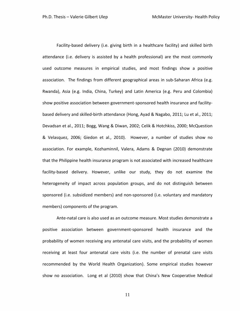
Facility-based delivery (i.e. giving birth in a healthcare facility) and skilled birth
attendance (i.e. delivery is assisted by a health professional) are the most commonly
used outcome measures in empirical studies, and most findings show a positive
association. The findings from different geographical areas in sub-Saharan Africa (e.g.
Rwanda), Asia (e.g. India, China, Turkey) and Latin America (e.g. Peru and Colombia)
show positive association between government-sponsored health insurance and facility-
based delivery and skilled-birth attendance (Hong, Ayad & Nagabo, 2011; Lu et al., 2011;
Devadsan et al., 2011; Bogg, Wang & Diwan, 2002; Celik & Hotchkiss, 2000; McQuestion
& Velasquez, 2006; Giedon et al., 2010). However, a number of studies show no
association. For example, Kozhaminnil, Valera, Adams & Degnan (2010) demonstrate
that the Philippine health insurance program is not associated with increased healthcare
facility-based delivery. However, unlike our study, they do not examine the
heterogeneity of impact across population groups, and do not distinguish between
sponsored (i.e. subsidized members) and non-sponsored (i.e. voluntary and mandatory
members) components of the program.
Ante-natal care is also used as an outcome measure. Most studies demonstrate a
positive association between government-sponsored health insurance and the
probability of women receiving any antenatal care visits, and the probability of women
receiving at least four antenatal care visits (i.e. the number of prenatal care visits
recommended by the World Health Organization). Some empirical studies however
show no association. Long et al (2010) show that China’s New Cooperative Medical

Ph.D. Thesis – Valerie Gilbert Ulep McMaster University- Health Policy
12
Systems (NCMS) has no detectable impact on the use of antenatal care. Similarly, Smith
& Sulbach (2008) demonstrate no detectable effects of health insurance on the
probability of receiving at least four antenatal care visits or receiving antenatal during
the first trimester in Ghana and Mali.
2.3.2 Impact of health insurance on health outcomes
There is little empirical evidence in the literature about the relationship between
health insurance and maternal and child health outcomes in low- and middle-income
countries, and research findings show contradictory results. We only found one study
that investigates the impact of government-sponsored insurance on maternal mortality
that addresses endogeneity. Chen & Jing (2012) find China’s NCMS has no detectable
impact on maternal mortality. Barros et al (2002) also find that neonatal mortality
decreased over time as insurance coverage expanded. However, their analysis is
descriptive, and is based on trend data.
Similarly, the evidence for the relationship between health insurance and
birthweight is limited in developing countries. We only found two studies. Cercone et al.
(2012) show that insured mothers in Costa Rica had a lower probability of having a low
birthweight newborn. In contrast, Gideon et al. (2010) find that insured mothers in
Colombia are more likely to have low birthweight. The authors do not explain this
unexpected finding.

Ph.D. Thesis – Valerie Gilbert Ulep McMaster University- Health Policy
13
2.4. Methods
In the impact evaluation literature (e.g., Heckman, Ichimura & Todd, 1997;
Caliendo & Kopenig, 2008; Imbens & Rubin, 2015; Smith & Sweetman, 2016), the effect
of a policy or program intervention is counterfactually described as the expected value
of the difference between a relevant outcome, Y, for each member i of the treated
group, (i.e. Yi1, which measures the health outcome of public insurance plan member i),
less the predicted outcome for that same individual if not treated (i.e. Yi0, the outcome
for the same member i if that person were not a member):
∆i= E[(Yi1) − (Yi0)]. (1)
While equation (1) cannot be estimated for any individual, its average can be
estimated using data from a successfully executed analysis with a sufficiently large
sample because the distribution of observed and unobserved characteristics for the
treated and non-treated groups are, on average, the same except for the treatment.
High-quality non-experimental sources of exogenous variation may also be used to
obtain estimates of causal impacts because, like well-executed experiments, they
provide treatment and comparison groups that, on average, have (perhaps conditional
on covariates) the same distributions of unobserved characteristics.
In observational data where there is no source of exogenous variation,
estimating program effects is not straightforward due to, especially, the presence of

Ph.D. Thesis – Valerie Gilbert Ulep McMaster University- Health Policy
14
selection into treatment which results in biased estimates if not adequately addressed.
At issue is that the treated and non-treated groups may differ on unobserved
dimensions that affect the outcome of interest. Under certain conditions, we can elicit
causal impact of the program by first estimating their counterfactual outcome of
members assuming they had not joined the national health insurance and then
differencing it from their observed outcome. The identifying assumption, sometimes
called conditional independence, is that the conditioning variables employed are
sufficient to render the distributions of unobserved variables in both the treatment and
comparison group approximately the same in large samples. Beyond the concept of
conditional independence, the potential outcome observed on one unit is also assumed
to be unaffected by the particular assignment to treatments of other units (known as
the Stable Treatment Value Assumption or SUTVA in statistics, and as the assumption of
no general equilibrium effects in economics).
In all three cases – experiments, quasi-experiments and situations without a
source of exogenous variation – if the identification is credible, the estimated difference
is commonly called the average treatment effect for the treated (ATET). If M=1 for
members and M=0 for non-members, then
∆i= E(Yi1 |Mi = 1) − E(Yi0 |Mi = 1) (2)

Ph.D. Thesis – Valerie Gilbert Ulep McMaster University- Health Policy
15
where the right-hand side is a counterfactual estimate of members’ expected outcome if
they had not been treated. The credibility of the impact estimate depends on the quality
of the counterfactual with well-executed randomized experiments or credible sources of
naturally occurring exogenous variation providing high-quality counterfactuals. For
estimates without a source of exogenous variation, that is for those relying on the
conditional independence assumption such as in this study, the identification of causal
impacts relies on conditioning on observable variables (using matching and/or
regression techniques) that render the treatment variable independent of the error
term.1 If the identifying assumption is thought not to be credible, then the estimates can
be interpreted as descriptive differences (i.e. conditional correlations that are not
causal) in outcomes conditional on observed characteristics.
In our context, E(Yi0|Mi = 1) is estimated using those who are not treated to
generate a counterfactual for those who are treated. In recent years, there have been
many methodological advances to address this problem, and propensity score matching
(PSM) is the most widely used technique in the impact evaluation literature when there
is not exogenous variation. A propensity score is the probability of joining the program
conditional on a given set of explanatory variables (Rosenbaum & Rubin, 1983). It can be
defined as e(X) = Probability(W=1|X). The propensity score is then used to balance
1 According to Heckman & Robb (1985), conventional selection bias approaches rely on strong distributional assumption. In practice, regressors (X’s) are assumed to be independent of the error term. However, in theory, they do not need to be independent. See Heckman & Robb (1985; 250). See also Smith & Sweetman (2016) for an interpretive introduction to these issues.
Ph.D. Thesis – Valerie Gilbert Ulep McMaster University- Health Policy
16
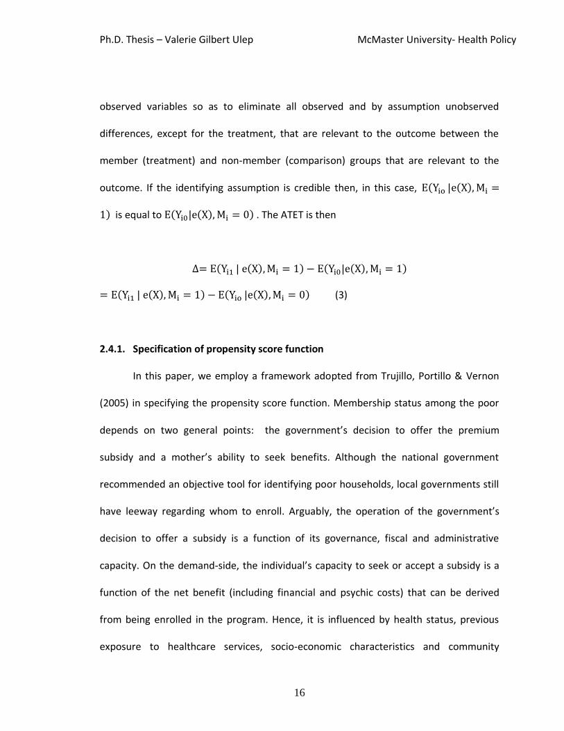
observed variables so as to eliminate all observed and by assumption unobserved
differences, except for the treatment, that are relevant to the outcome between the
member (treatment) and non-member (comparison) groups that are relevant to the
outcome. If the identifying assumption is credible then, in this case, E(Yio |e(X), Mi =
1) is equal to E(Yi0|e(X), Mi = 0) . The ATET is then
∆= E(Yi1 | e(X), Mi = 1) − E(Yi0|e(X), Mi = 1)
= E(Yi1 | e(X), Mi = 1) − E(Yio |e(X), Mi = 0) (3)
2.4.1. Specification of propensity score function
In this paper, we employ a framework adopted from Trujillo, Portillo & Vernon
(2005) in specifying the propensity score function. Membership status among the poor
depends on two general points: the government’s decision to offer the premium
subsidy and a mother’s ability to seek benefits. Although the national government
recommended an objective tool for identifying poor households, local governments still
have leeway regarding whom to enroll. Arguably, the operation of the government’s
decision to offer a subsidy is a function of its governance, fiscal and administrative
capacity. On the demand-side, the individual’s capacity to seek or accept a subsidy is a
function of the net benefit (including financial and psychic costs) that can be derived
from being enrolled in the program. Hence, it is influenced by health status, previous
exposure to healthcare services, socio-economic characteristics and community

Ph.D. Thesis – Valerie Gilbert Ulep McMaster University- Health Policy
17
characteristics. In the estimation of propensity scores, we use a logit regression model
for the semi-parametric matching, and a kernel smoothing regression for the non-
parametric matching. The logit regression model is:
Pr (Enrolled = 1) = F(a + b1X1 + b2X2 + b3X3) (4)
Where F is the cumulative distribution function for the logistic distribution, “a” is an
intercept, the “Xn” are vectors of variables with “n” indexing the three groups of
characteristics, and the “b” are coefficients to be estimated.
2.4.2. Matching estimators
After estimating the propensity scores using a logit regression model, we
investigate whether the average propensity score and the mean of each explanatory
variable are approximately equal for members and non-members. In practice, a variety
of matching techniques are commonly used including nearest neighbor, stratification
and kernel weighting. Caliendo & Kopenig (2008), and Frolich, Huberg & Wiesenfarth
(2015) provide details about the advantages and disadvantages, estimation procedures,
conditions and assumptions for each matching method. In this study, we employ local
linear matching (LLM), which is a non-parametric estimator that uses a prediction from a
local linear regression for each counterfactual estimate. One of the advantages of using
LLM is lower variance as more information is used (Caliendo & Kopenig, 2008). We then

Ph.D. Thesis – Valerie Gilbert Ulep McMaster University- Health Policy
18
check if the means of the covariates are equal for member and non-members are
balanced using t-tests. If the means are not statistically significantly different, or if the
difference is less than 10 percent, the means of the covariates are regarded as
approximately equal for members and non-members.
Inference for the ATET uses non-parametric percentile-t clustered bootstrapping
with 999 replications to estimate the p-values and confidence intervals. We re-center
each bootstrap t-statistic around the sample’s coefficient estimate (Cameron & Trivedi,
2010; Signh & Xie, 2010). Cluster bootstrapping is required since we include province-
level (macro) variables in regressions using individual-level data. Cluster bootstrapping
accounts for intra-cluster (intra-province) correlations that might otherwise render our
standard error estimates inconsistent.
As an alternative to semi-parametric PSM, we also use inverse probability
weighting (IPW). IPW assigns greater weight to those comparison group members with
higher estimated propensity scores (Hirano & Imbens, 2001; Imbens, 2004). We derive
weights from the propensity score, e (X) using the following IPW estimator:
△= N−1 ∑MiYi
e(X)− N−1 ∑
(1−Mi )Yi
1−e(X)
Ni=1
Ni=1 (4)
where N is the total number of subjects. M is the treatment and Y is the outcome.
The aforementioned estimators use a parametric logit regression model to
estimate the propensity score. Although parametric models can provide estimates of the

Ph.D. Thesis – Valerie Gilbert Ulep McMaster University- Health Policy
19
true propensity score, they do not usually guarantee suitable approximations.
Estimators based on a non-parametric propensity score have demonstrated the lowest
possible asymptotic variance (Li, Racine & Woolridge, 2008; Hahn, 1998). In Monte
Carlo trials, Frolich, Huberg & Wiesenfarth (2015) find that non-parametric regression
outperforms all other semi-parametric estimators in estimating ATET. As a third option,
we therefore follow the method of Li, Racine & Woolridge (2008) and Hall, Racine & Li
(2007) in estimating the propensity scores using a kernel smoothing non-parametric
regression model.
For all three estimators, we estimate the effect of national health insurance on
the abovementioned maternal and infant health outcomes across subgroups. These
include the difference in the ATET between the 1st and 2nd wealth quintiles, the
difference between urban and rural, the difference between uniparous and multiparous,
as well as the difference between low and high educational attainment. We also
calculate the effect size (Cohen’s d) to examine the clinical importance of our estimates.
Cohen’s d is calculated using the following formula: ([MeanGroup1- Mean Group2)]/SD pooled.).
Cohen arbitrarily classifies effect size as small, medium or large using the cut-off values
of 0.2, 0.5 and 0.80, respectively (Cohen, 1988).
2.4.3. Data
We use the nationally representative 2013 National Demographic and Health
Survey (NDHS) conducted by the National Statistics Office of the Philippines. The NDHS

Ph.D. Thesis – Valerie Gilbert Ulep McMaster University- Health Policy
20
has households’, individuals’ and women’s modules; 14,808 households were
interviewed with a 99.4 percent response rate. Among those interviewed, 16, 437
women of reproductive age were identified as eligible respondents for the women’s
module with a 98.4 percent response rate. It is possible that more than one woman in a
household were interviewed. On average, there are 2 women of reproductive age per
household in the Philippines (Philippine Statistical Authority and ICF International 2014).
In this study, the household and women’s modules are merged. We also employ
aggregate data such as the prevalence of poverty, a governance index,2 public health
expenditure per capita and the number of hospital beds per capita for the 81 provinces
from the websites of the Philippine Statistical Authority and Department of Health.
Because it is more policy relevant, the study focuses only on poor mothers who
experienced at least one pregnancy in the three years prior to the survey. Mothers
belonging to the first and second quintiles of wealth scores are considered poor and
mothers belonging to higher socio-economic quintiles are excluded from the sample.
The variable wealth score was generated by the Philippine Statistical Authority using
principal component analysis of selected tangible household assets. The sample size for
2 Governance index (GI) is a weighted arithmetic average of the Economic Governance Index (EGI), the Political Governance Index (PGI) and the Administrative Governance Index (AGI). The Economic Governance Index is calculated using fiscal-related indicators such as revenue collection, social services expenditures, and macro-economic indicators (e.g. inflation, unemployment, poverty gap). The Political Governance Index (PGI) is calculated using the following indicators: crime solution efficiency and voter’s turn out rates. The Administrative Governance Index is calculated using school-related (e.g. drop-out rates, classroom-student ratio) and road, electricity and telephone-density indicators. The Philippine Statistical Authority officially releases the GIs of provinces.
Ph.D. Thesis – Valerie Gilbert Ulep McMaster University- Health Policy
21
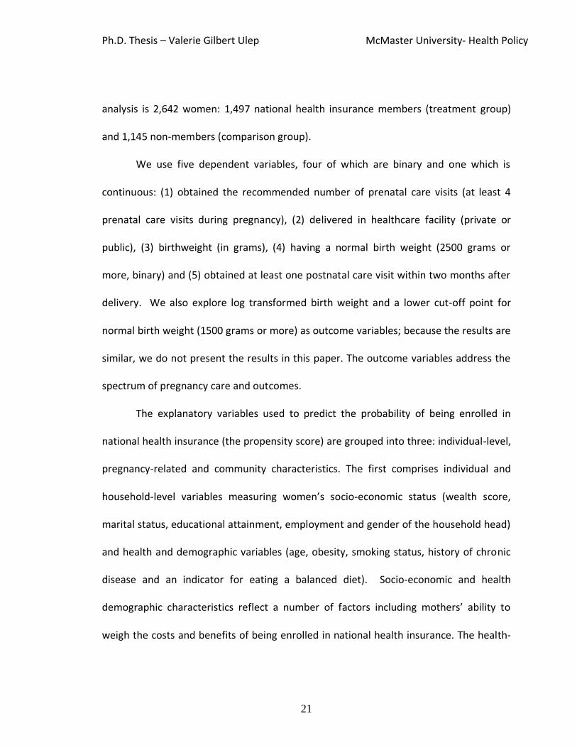
analysis is 2,642 women: 1,497 national health insurance members (treatment group)
and 1,145 non-members (comparison group).
We use five dependent variables, four of which are binary and one which is
continuous: (1) obtained the recommended number of prenatal care visits (at least 4
prenatal care visits during pregnancy), (2) delivered in healthcare facility (private or
public), (3) birthweight (in grams), (4) having a normal birth weight (2500 grams or
more, binary) and (5) obtained at least one postnatal care visit within two months after
delivery. We also explore log transformed birth weight and a lower cut-off point for
normal birth weight (1500 grams or more) as outcome variables; because the results are
similar, we do not present the results in this paper. The outcome variables address the
spectrum of pregnancy care and outcomes.
The explanatory variables used to predict the probability of being enrolled in
national health insurance (the propensity score) are grouped into three: individual-level,
pregnancy-related and community characteristics. The first comprises individual and
household-level variables measuring women’s socio-economic status (wealth score,
marital status, educational attainment, employment and gender of the household head)
and health and demographic variables (age, obesity, smoking status, history of chronic
disease and an indicator for eating a balanced diet). Socio-economic and health
demographic characteristics reflect a number of factors including mothers’ ability to
weigh the costs and benefits of being enrolled in national health insurance. The health-
Ph.D. Thesis – Valerie Gilbert Ulep McMaster University- Health Policy
22
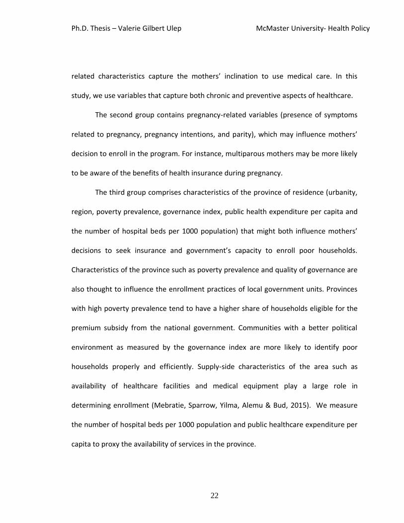
related characteristics capture the mothers’ inclination to use medical care. In this
study, we use variables that capture both chronic and preventive aspects of healthcare.
The second group contains pregnancy-related variables (presence of symptoms
related to pregnancy, pregnancy intentions, and parity), which may influence mothers’
decision to enroll in the program. For instance, multiparous mothers may be more likely
to be aware of the benefits of health insurance during pregnancy.
The third group comprises characteristics of the province of residence (urbanity,
region, poverty prevalence, governance index, public health expenditure per capita and
the number of hospital beds per 1000 population) that might both influence mothers’
decisions to seek insurance and government’s capacity to enroll poor households.
Characteristics of the province such as poverty prevalence and quality of governance are
also thought to influence the enrollment practices of local government units. Provinces
with high poverty prevalence tend to have a higher share of households eligible for the
premium subsidy from the national government. Communities with a better political
environment as measured by the governance index are more likely to identify poor
households properly and efficiently. Supply-side characteristics of the area such as
availability of healthcare facilities and medical equipment play a large role in
determining enrollment (Mebratie, Sparrow, Yilma, Alemu & Bud, 2015). We measure
the number of hospital beds per 1000 population and public healthcare expenditure per
capita to proxy the availability of services in the province.

Ph.D. Thesis – Valerie Gilbert Ulep McMaster University- Health Policy
23
2.5. Results
Table 2.1 displays the unconditional means of these outcome variables and tests
whether they differ by health insurance membership status. The percent of mothers
with both the recommended number of visits and facility-based delivery are higher
among members compared to non-members, but the means for postnatal visits and
birthweight are not statistically significantly different. The smaller sample size for
birthweight is due to a large number of missing observations. Table 2.2 presents a
descriptive analysis of health insurance membership status and individual explanatory
variables.
For semi-parametric propensity score matching, we estimate the propensity
score of being enrolled in the national health insurance using a logit regression model.
This is followed by matching the treatment and comparison groups using local linear
regression to re-weight the comparison group. One necessary condition for matching to
work is common support in the data for the two groups (i.e. overlapping propensity
score distributions). After exploring our data, we impose common support by trimming
the one percent of treated observations for which the propensity score density of the
comparison is lowest; fourteen observations are removed because there are not
comparable comparison group members. Lastly, we check the quality of matching by
assessing the extent of balancing achieved on the two matched samples (i.e., t-tests for
equality of means in the two samples). Table 2.3 shows that the characteristics of
covariates of health insurance members (treatment) and non-members (comparison)

Ph.D. Thesis – Valerie Gilbert Ulep McMaster University- Health Policy
24
are balanced as ascertained by statistically insignificant p-values (except for mother’s
education) and less than 10 percentage bias in all covariates, which is the most
commonly used cut-off point.
Table 2.4 presents the ATET of health insurance for different maternal and infant
health outcomes using three estimators. Out of the five outcome variables, only the
three utilization measures are statistically significantly different for the member and
non-member groups: recommended prenatal care visits, healthcare facility-based
delivery and postnatal care visit. Poor mothers enrolled in the national health insurance
display a higher probability of obtaining the number of recommended prenatal care
visits, of delivering newborns in healthcare facilities and obtaining at least one postnatal
care visit within two months after delivery (except for postnatal care visit using semi-
parametric estimator for which the ATET is not statistically different from zero).
Turning to birthweight (see the discussion section regarding sample size), the
coefficients are all statistically insignificant; this is consistent across the three estimators
of ATET. Further, the point estimates suggest national health insurance coverage
actually reduces birthweight. The large standard error and wide confidence intervals of
the average treatment effects on birthweight might be in part attributable to small
sample size. Of the 2, 642 sample, 792 were excluded due to non-response.
We also estimate the effect of national health insurance coverage across
potentially important subgroups. These include the difference in the ATET between the
first and second wealth quintiles, urban and rural geographies, uniparous and

Ph.D. Thesis – Valerie Gilbert Ulep McMaster University- Health Policy
25
multiparous mothers, as well as mothers with low and high educational attainment.
Results show that in all subgroups, the effects of national health insurance on
recommended prenatal care visits, healthcare facility-based delivery and postnatal care
visit are each statistically significant for at least one of the three ATET estimators (Table
2.5). However, the effect of national health insurance on birthweight (both continuous
and binary specifications) in all subgroups is consistently statistically insignificant across
the three estimators. In urban areas, the ATET of national health insurance on
healthcare facility-based delivery is higher than in rural. The ATET of national health
insurance on the recommended number of prenatal care visits is also higher among
mothers belonging to the first wealth quintile compared to the second. Similarly, the
ATET for recommended prenatal care visits is also higher among mothers with low
educational attainment. Among uniparous mothers, the ATET on healthcare facility-
based delivery is larger compared to multiparous mothers, and the ATET of national
health insurance on recommended prenatal care visits is smaller. Although it may
appear that there are differences in the point estimates between subgroups, these are
statistically insignificant as witnessed by the overlapping confidence intervals.
For the three estimators to provide results that may be interpreted as causal, an
assumption that is referred to using terms such as unconfoundedness or conditional
independence is required. It means that selection bias is only due to observed
characteristics (Imbens and Rubin, 2015). We argue that the NDHS includes the variables
Ph.D. Thesis – Valerie Gilbert Ulep McMaster University- Health Policy
26
needed for the empirical strategy to, at least approximately, satisfy this condition in
accordance with the framework by Trujillo, Portillo & Vernon (2005).
2.6. Discussion
Our study reveals that poor mothers who are covered with the Philippines’
national insurance program have a higher probability of obtaining the recommended
number of prenatal care visits, of giving birth in a healthcare facility and of having a
postnatal care visit within two months after delivery. However, there is no statistically
significant effect on birthweight. There are several explanations for why the program did
not produce a health improvement on this dimension. First, public health insurance can
increase healthcare utilization, but healthcare services may not be a major determinant
of health status (e.g., Smith, 1999; Chen et al., 2007). The social determinants of health
framework suggests that health is determined not only by healthcare interventions but
by a plethora of physical, environmental and other socio-economic conditions (Smith,
1999; Evans & Stoddart, 1990). Second, the lack of program effect on health status
might be a reflection of the poor quality of healthcare services. Limited policy attention
is given to the quality of healthcare services especially in government-run hospitals and
clinics where poor mothers usually seek maternal and childcare services. Hence, despite
the higher quantity, the poor quality of healthcare services may have limited the effects
on health status (Chen et al., 2007).

Ph.D. Thesis – Valerie Gilbert Ulep McMaster University- Health Policy
27
Our study also shows that the effect of the national health insurance program is,
on two dimensions, somewhat larger for the most vulnerable population. The effect of
the program on recommended prenatal care and postnatal visits is larger among
mothers in the poorest quintile and among mothers with low education. In contrast,
while positive for our entire sample, the effect on healthcare facility-based delivery is
statistically insignificant for this subgroup. Healthcare facility-based delivery might be
prohibitively expensive because of the high non-medical and medical costs incurred
outside the insurance benefit (e.g. transportation costs). More importantly, the lack of
effect of the program on healthcare facility-based delivery may also signal the lack of
healthcare facilities in poor areas. This is consistent with the lack of a significant effect
of health insurance on facility-based delivery among mothers living in rural areas.
Although there is an interesting pattern in the point estimates, the overlapping
confidence intervals suggest that the differences in ATET between subgroups are not
statistically significant. We conducted an ex-post power calculation to determine if the
statistical insignificance can be attributed to the small sample size. Our calculation
indicated that with our current sample size the power of the test is low (less than
80%);hence, we cannot make airtight inferences.
From clinical and economic standpoints, it is important to assess not only
statistical significance but also how quantitatively meaningful the average treatment
effects of the program are. Unfortunately, clinical importance is not always well-defined.
As described above, one common, if ad hoc, the method for assessing a “minimal

Ph.D. Thesis – Valerie Gilbert Ulep McMaster University- Health Policy
28
clinically important difference” or a “clinically meaningful difference” is to calculate
Cohen’s d. By this metric, the effect of the program on prenatal care visits is clinically
important. The Cohen’s d from the IPW and non-parametric estimators are above the
cut-off point recommended for an effect size (ATET) to be considered clinically
important (a Cohen’s d of ≥ 0.2 is considered clinically important). In contrast, the
Cohen’s d for healthcare facility-based delivery and postnatal care visits is < 0.2 for all
estimators. This suggests that even though the ATET estimates for healthcare facility-
based delivery and a postnatal care visit are statistically significant, they may not be
“clinically” important. Comparing across groups, while the effect sizes of the program
on optimal prenatal care visits in the lowest wealth quintile and low education groups
are clinically important, they are not for the second lowest wealth quintile and high
education groups. The effect sizes on other outcomes are not clinically important in
both wealth quintile and education groups.
Despite the judgment of potential importance for the recommended prenatal
care visit following from Cohen’s d, the lack of a statistically significant effect of the
program on birthweight suggests that the overall effect does not have much policy
relevance – at least not on this important dimension. However, some might argue that
this statistical insignificance might be due to the small sample size – assuming an
“important” effect to be quite modest given that our point estimate is quite close to
zero. We, therefore, conducted an ex-post power calculation to determine how large
the sample size would need to be to detect a clinically important difference. In the case

Ph.D. Thesis – Valerie Gilbert Ulep McMaster University- Health Policy
29
of the proportion with normal birthweight (i.e., above 2500 grams), we would need a
sample size of approximately 1, 052 to detect a clinically important difference. Assuming
a 0.20 Cohen’s d, the clinically important difference between health insurance members
and non-members is 0.10. However, we observed a statistically insignificant ATET of
about 0.01 with our current sample size (n=1.810). The difference between the observed
ATET and the clinically important ATET (0.01 vs. 0.10) is statistically significant (p
value=0.000). Our interpretation is that the “true” impact of health insurance on
birthweight is zero to trivially small. If there were a clinically important difference in the
proportion of normal birthweight between member and non-member, the model should
have detected it with our current sample size.
Overall, our study supports the literature in questioning the effectiveness of
health insurance, or at least these particular insured services, as the only policy tool for
improving population health status, especially in developing countries. Also the results
support further discussions on the feasibility of health insurance as a conduit for the
delivery of effective interventions in the health insurance benefit plan.
In terms of research implications, our study calls for a more rigorous impact
evaluation of health insurance in developing countries. In spite of our efforts to use
propensity score matching to identify the causal relationship between the national
health insurance program and maternal and child outcomes, we might have not fully
met the assumption of unconfoundedness. Our results might, therefore, be interpreted
by some readers as identifying correlations (or covariance) conditional on the regressors

Ph.D. Thesis – Valerie Gilbert Ulep McMaster University- Health Policy
30
in our model rather than as causal parameters. While this modifies the interpretation of
our results, we think that the questions about the program’s effectiveness in improving
birthweight – a common and useful proxy for health status – remain. An implication of
this argument is that governments should engage in a well-designed community
effectiveness experiments (or, more broadly, introduce some source of exogenous
variation in treatment) to evaluate this important initiative. Such experiments would
convincingly reduce the effects of selection bias and generate valid evidence on the
causal impacts of programs such as the one studied here.
Lastly, there is also a limitation inherent in our data that might affect the validity
of our estimates. In this study, we used self-reported birth weight as a child health
outcome and, given the low response rate (792 respondents out of 2, 642 did not
report), aside from measure error our estimates might be biased because of who
responds. There is a systematic difference between mothers who reported birthweight
and those who did not. Mothers who did not report birthweight are more likely from
the poorest wealth quintile, have low educational attainment, and living in rural areas.
2.7. Conclusion
Our key conclusion is that the Philippines’ national health insurance program
moderately increases the utilization of healthcare services among poor women during
pregnancy. This impact is somewhat larger for the most vulnerable population --
mothers in the poorest quintile and/or with low education. With these findings, we can

Ph.D. Thesis – Valerie Gilbert Ulep McMaster University- Health Policy
31
say that the Philippine national health insurance program improved healthcare access
among the poor, which supports the main thrust of UHC. However, the lack of
detectable impact on the health status of infants as measured by birthweight for any
group suggests that health insurance expansion alone might not be a sufficient to
improve health outcomes. A policy implication of our results is that it is important for
less developed countries like the Philippines to complement health insurance expansion
with other effective interventions.

Ph.D. Thesis – Valerie Gilbert Ulep McMaster University- Health Policy
32
2.8. Reference
Barros C., Victora G., Barros J., Santos S., Albernaz E., Matijasevich A et al. (2005). The
challenge of reducing neonatal mortality in middleincome countries: findings from
three Brazilian birth cohorts in 1982, 1993, and 2004. Lancet, 365, pp. 847-54
Bogg L., Huang K., Long Q., Shen Y. & Hemminki E. (2010). Dramatic increase of cesarean
deliveries in the midst of health reforms in rural China. Social Science and Medicine,
pp. 1544-9.
Caliendo, M. & Kopenig, S. (2008). Some practical guidance for the implementation of
propensity score matching. Journal of Economic Surveys, 22(1), pp. 31-72.
Cameron, A. & Trivedi, P. (2010). Microeconometrics using STATA. STATA Press.
Cotlear, D., Nagpal, S., Smith, O., Tandon, T. & Cortez, D. (2013). Going Universal: How
24 Developing countries are implementing UHC reforms from the Bottom up.
Washington DC: World Bank.
Celik, Y. & Hotchkiss, D. (2000). The socio-economic determinants of maternal health
care utilization in Turkey, 50(12), 1797-1809.
Cercone J., Pinder E., Jimenez J. & Briceno R. (2010). Impact of health insurance on
access, use, and health status in Costa Rica. In: Escobar M-L, Griffin CC, Shaw RP,
editors. The impact of health insurance in low- and middle-income countries.
Washington, DC: Brookings Institution Press, pp. 89-105.
Chen, L., Yip, W., Chang, M., Lin, H., Lee, S., Chiu, Y. & Lin, Y. (2007). The effects of
Taiwan’s National Health Insurance on access and health status of the elderly.

Ph.D. Thesis – Valerie Gilbert Ulep McMaster University- Health Policy
33
Health Economics, 16(3), 223–242.
Chen, Y. & Jin, Z. (2012). Does health insurance coverage lead to better health and
educational outcomes? Evidence from rural China. Journal of Health Economics,31,
pp. 1-14.
Cohen, J. (1988). Statistical power analysis for the behavioral sciences. Second ed.
Hillsdale, NJ: Lawrence Earlbaum Associates.
Comfort, A., Peterson, L. & Hatt, L. (2013). Effect of health insurance on the use and
provision of paternal health services and maternal and neonatal health outcomes:
A systematic review. Journal Health Population Nutrition, 31(4), pp. 81-105.
Devadasan N., Criel B., Van Damme W., Manoharan S., Sarma P., Van der Stuyft P.
(2010). Community health insurance in Gudalur, India, increases access to hospital
care. Health Policy Planning, 25:145-54.
Frolich, M., Huberg, M. & Wiesenfarth, M. (2015). The finite sample performance of
semi- and nonparametric estimators for treatment effects and policy evaluation.
Bonn: IZA Working Paper No. 8756.
Giedon, U., Alfonso, E. & Diaz, Y. (2013). The impact of universal coverage schemes in
the developing world: A review of the existing evidence. Washington DC: World
Bank.
Giedion U., Florez C., Diaz Y., Alfonso E., Pardo R &, Villar M. (2010). Colombia’s big bang
health insurance reform. In: Escobar M-L, Griffin CC, Shaw RP, editors. The impact
of health insurance in low- and middle-income countries. Washington, DC:

Ph.D. Thesis – Valerie Gilbert Ulep McMaster University- Health Policy
34
Brookings Institution Press, pp. 155-77.
Hahn, J. (1998). On the role of the propensity score in efficient semiparametric
estimation of average treatment effects. Econometrica, 66(2), pp. 315–331.
Hall, P., Racine, J. & Li, Q. (2007). Nonparametric estimation of regression functions in
the presence of irrelevant regressors. Review of Economics and Statistics, 89(7), pp.
784–89.
Heckman, J., Ichimura, H. & Todd, P. (1997). Matching as an econometric evaluation
estimator: evidence from evaluating a job training program. Review of Economics
and Statisitcs, 64(4), pp. 605-54.
Hong R., Ayad M. & Ngabo F. (2011). Being insured improves safe delivery practices in
Rwanda. J Community Health;36, pp. 779-84.
Hirano, K. & Imbens, G. (2001). Estimation of causal effects using propensity score
weighting: an application to data on right heart catheterization. Health Services
Outcomes Research Methodology, 2(3), pp. 259-78.
Imbens, G. & Rubin, D. (2015). Causal Inference for Statistics, Social, and Biomedical
Sciences: An Introduction. New York: Cambridge University Press.
Imbens, G. (2004). Non-parametric estimation of average treatment effects under
exogeniety: a review. Review of Economics and Statistics, 86(1), pp.4-29.
Kozhimannil, K., Valera, M., Adams, A. & Degnan, D. (2009). The population-level
impacts of a national health insurance program and franchise midwife clinics on
achievement of prenatal and delivery care standards in the Philippines. Health

Ph.D. Thesis – Valerie Gilbert Ulep McMaster University- Health Policy
35
Policy, 92(1), pp. .55-64.
Lagarde, M. & Palmer, N. (2006). Evidence from systematic reviews to inform decision
making regarding financing mechanisms that improve access to health services for
poor people. Khon Kaen, Thailand: Alliance for Health Policy and System Research.
Lavado, R., Ulep, V., Pantig, I., dela Cruz, N., Aldeon, M. & Oriz, D. (2011). Profile of
private hospitals in the Philippines. Makati: PIDS Working Paper no. 2011-5.
Li, Q., Racine, J. & Woolridge, J. (2008). Estimating average treatment effects with
continuous and discrete covariates: the case of swan-ganz catheterization.
American Economic Review, 98(2), pp. 357–362.
Lu C., Chin B, Lewandowski J., Basinga P., Hirschhorn L., Hill K. et al. (2012). Towards
universal health coverage: an evaluation of Rwanda Mutuelles in its first eight
years. PLoS One
McQuestion, M & Velasquez, A. (2006). Evaluating program effects on institutional
delivery in Peru. Health Policy, 77(22), pp.221-232.
Mebratie, A., Sparrow, R., Yilma, Z et al. (2015). Enrollment in Ethiopia’s community-
based health insurance scheme. World Development, 74, 58–76.
Mensah, J., Oppong, J. & Schmidt, C. (2010). Ghana’s national health insurance scheme
in the context of the health MDGs: an empircal evaluation using Propensity Score
Matching. Health Economics, 19, pp. 95-106.
Philippine Health Insurance Corporation (2003). PhilHealth Maternity Care Package for
normal sontaneous delivery. [Online] Mandaluyong City: Philippine Health

Ph.D. Thesis – Valerie Gilbert Ulep McMaster University- Health Policy
36
Insurance Corporation Available at: www.philhealth.gov.ph [Accessed 5 June 2015].
Philippine Statistical Authority, ICF International (2014). 2013 Philippines National
Demographic and Health Surveys: key findings. Manila, Philipines and Bethesda,
Maryland: PSA and ICF International.
Picazo, O., Ulep, V. & dela Cruz, N. (2013). The puzzle of economic growth and stalled
health improvement in the Philippines. Makati: PIDS Working Paper no. 2013-7.
Republic of the Philippines (1995). National Health Insurance Act of 1995. Metro Manila.
Romualdez, R., dela Rosa, J., Flavier, J., Quimbo, S., Hartigan-Go, K., Lagrada, L. & David,
D. (2011). The Philippine health system review. Geneva: World Health
Organization.
Rosenbaum, P. & Rubin , D. (1983). The central role of propensity score in observational
studies for causal effects. Biometrika, 70(1), pp. 41-50.
Smith, J. (1999). Healthy bodies and thick wallets: The dual relation between health and
economic status. Journal of Economic Perspectives, 13(2), pp. 145-66.
Smith, J., Sweetman, A. (2016). Viewpoint: Estimating the causal effects of policies and
programs. Canadian Journal of Economics, forthcoming.
Smith K. & Sulzbach S. (2008). Community-based health insurance and access to
maternal health services: evidence from three West African countries. Social
Science & Medicine. 66, pp. 2460–73.
Silfverberg, R. (2014). The Sponsored Program of the Philippine National Health
Insurance – analyses of the actual coverage and variations across regions and

Ph.D. Thesis – Valerie Gilbert Ulep McMaster University- Health Policy
37
provinces. Makati: Philippine Institute for Development Studies.
Trujillo, A., Portillo, J. & Vernon, J. (2005). The impact of subsidized health insurance for
the poor: evaluating the Colombian experience using Propensity Score Matching.
International Journal of Health Care Financing and Economics, 5, pp. 211-39.
Ulep, V. & dela Cruz, N. (2014). Analysis of out-of-pocket payments in the Philippines.
Makati: Philippine Institute for Development Studies Working Paper no.15.
United Nations. (2017). The 2030 Agenda for sustanainable developoment. New York
World Health Organization. (2010). Health systems financing: a path to universal
coverage. Geneva, Switzerland.
World Health Organization (2015). Health in 2015: from MDGs, Millennium
Development Goals to SDGs, Sustainable Development Goals. Geneva: World
Health Organization.
World Health Organization and International Bank for Reconstruction and Development
/World Bank (2017). Tracking universal health coverage: 2017 global monitoring
report. Geneva, World Health Organization.

Ph.D. Thesis – Valerie Gilbert Ulep McMaster University- Health Policy
38
Table 2.1. Unconditional probability and means of the outcomes, by health insurance membership status
Member (n) Non-member (n)
% of women with recommended number of prenatal visit
0.80 (1,497) 0.73 (1,145)*
% women who delivered in healthcare facility
0.49 (1,496) 0.47 (1,145)*
% women with normal birthweight children
0.78 (774) 0.78 (1,036)
Mean birthweight (in grams) 2952.2 (1,036) 2929.2 (774)
% of women with post-natal visits within two months after delivery
0.86 (1,496) 0.84 (1,141)
Notes:
1. Source of data: 2013 National Demographic and Health Survey 2. The number of observations are in parenthesis (n). The lower sample size for
birthweight is due to missing observation and non-response. 3. Recommended number of prenatal visit means at least four visits, while post-natal visit
means at least one visit to a health facility within two months after delivery. 4. Birthweight in grams 5. Asterisk (*) means there is statistically significant difference (p<0.05). Chi-square or t-
test

Ph.D. Thesis – Valerie Gilbert Ulep McMaster University- Health Policy
39
Table 2.2. Descriptive statistics of selected variables, by health insurance membership status
Explanatory Variables Member Non-member p value Age during pregnancy (Mean) 1 29.99 26.26 0.000 Currently working (%)2 0.51 0.39 0.000 Marital status
Single (%) 0.01 0.03 0.002 Married (%) 0.97 0.93 0.000 Others (%) 0.02 0.04 0.002
Wealth index scores1 -106,488.10 -99,298.49 0.001 Mother’s education
No education (%) 0.02 0.05 0.001 Primary (%) 0.36 0.34 0.220 Secondary (%) 0.49 0.52 0.250 Tertiary (%) 0.12 0.10 0.060
Female as head2 0.07 0.10 0.007 Experience symptoms during pregnancy2 0.66 0.67 0.530 Parity (number of births) 1 4.15 2.97 0.000 Pregnancy intentions
Wanted (%) 0.69 0.73 0.016 Unwanted (%) 0.14 0.17 0.130 Mistimed (%) 0.17 0.10 0.000
Current smoker (%)2 0.05 0.06 0.130 Obese (%)2 0.10 0.09 0.300 Eat balanced-diet (%)2 0.23 0.22 0.700 Family history of chronic illness (%)2 0.28 0.26 0.210 Living in urban (%)2 0.19 0.29 0.000 Poverty prevalence of the province1 36.57 35.95 0.350 Governance index of the province4, 116.97 119.62 0.000 Public health expenditure of the province 1 145.77 148.86 0.570 Number of hospital bed per 1000 population1 0.86 0.86 0.930
Notes:
1. Continuous variables. The values are expressed as means 2. Binary variable. The values are expressed as proportions 3. Region variable is not included to maximize space 4. The higher the governance index, the better governance level.
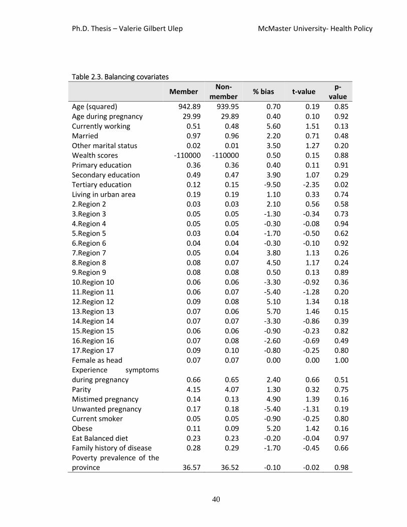
Ph.D. Thesis – Valerie Gilbert Ulep McMaster University- Health Policy
40
Table 2.3. Balancing covariates
Member
Non-member
% bias t-value p-
value Age (squared) 942.89 939.95 0.70 0.19 0.85 Age during pregnancy 29.99 29.89 0.40 0.10 0.92 Currently working 0.51 0.48 5.60 1.51 0.13 Married 0.97 0.96 2.20 0.71 0.48 Other marital status 0.02 0.01 3.50 1.27 0.20 Wealth scores -110000 -110000 0.50 0.15 0.88 Primary education 0.36 0.36 0.40 0.11 0.91 Secondary education 0.49 0.47 3.90 1.07 0.29 Tertiary education 0.12 0.15 -9.50 -2.35 0.02 Living in urban area 0.19 0.19 1.10 0.33 0.74 2.Region 2 0.03 0.03 2.10 0.56 0.58 3.Region 3 0.05 0.05 -1.30 -0.34 0.73 4.Region 4 0.05 0.05 -0.30 -0.08 0.94 5.Region 5 0.03 0.04 -1.70 -0.50 0.62 6.Region 6 0.04 0.04 -0.30 -0.10 0.92 7.Region 7 0.05 0.04 3.80 1.13 0.26 8.Region 8 0.08 0.07 4.50 1.17 0.24 9.Region 9 0.08 0.08 0.50 0.13 0.89 10.Region 10 0.06 0.06 -3.30 -0.92 0.36 11.Region 11 0.06 0.07 -5.40 -1.28 0.20 12.Region 12 0.09 0.08 5.10 1.34 0.18 13.Region 13 0.07 0.06 5.70 1.46 0.15 14.Region 14 0.07 0.07 -3.30 -0.86 0.39 15.Region 15 0.06 0.06 -0.90 -0.23 0.82 16.Region 16 0.07 0.08 -2.60 -0.69 0.49 17.Region 17 0.09 0.10 -0.80 -0.25 0.80 Female as head 0.07 0.07 0.00 0.00 1.00 Experience symptoms during pregnancy 0.66 0.65 2.40 0.66 0.51 Parity 4.15 4.07 1.30 0.32 0.75 Mistimed pregnancy 0.14 0.13 4.90 1.39 0.16 Unwanted pregnancy 0.17 0.18 -5.40 -1.31 0.19 Current smoker 0.05 0.05 -0.90 -0.25 0.80 Obese 0.11 0.09 5.20 1.42 0.16 Eat Balanced diet 0.23 0.23 -0.20 -0.04 0.97 Family history of disease 0.28 0.29 -1.70 -0.45 0.66 Poverty prevalence of the province 36.57 36.52 -0.10 -0.02 0.98

Ph.D. Thesis – Valerie Gilbert Ulep McMaster University- Health Policy
41
Governance index of the province 116.97 117.35 -1.90 -0.54 0.59 Public health expenditure of the province 145.77 146.30 -0.50 -0.14 0.89 Number of hospital bed per 1000 population 0.86 0.87 -3.80 -1.13 0.26
Note:
1. The values for member and non-member are expressed as either means (continuous variable) or proportion (binary variable).
2. We impose less than 10 percent as acceptable percentage bias 3. t- value and p-value use to compare the equality of two means

Ph.D. Thesis – Valerie Gilbert Ulep McMaster University- Health Policy
42
Table 2.4. Average treatment effects of health insurance on maternal health outcomes
Outcomes
Semi-parametric PSM (local linear regression)
IPW Non-parametric
ATET 95CI Effect size ATET 95CI Effect size ATET 95CI Effect size
Recommended prenatal care visit
0.07*** 0.06 0.12 0.16 0.12* 0.08 0.17 0.27# 0.11* 0.08 0.14 0.25#
Facility-based delivery 0.06*** 0.02 0.10 0.13 0.08* 0.04 0.12 0.17 0.05 0.02 0.07 0.10
Birth weight (in grams) -29.88 -100.45 50.56 -0.03 -35.20 -129.56 69.83 -0.04 -7.44 -42.93 30.75 -0.01
Birth weight (binary) 0.01 -0.02 0.04 0.012 -0.00 -0.04 0.04 -0.01 0.00 -0.02 0.02 0.01
Postnatal visit 0.03 0.00 0.06 0.07 0.03* 0.00 0.06 0.08 0.05* 0.00 0.09 0.13
* p<0.05, ** p<0.01, *** p<0.001,
Note:
1. ATET means average treatment effect of the treated
2. Bootstrapped standard error from 999 replications taking into account the clustering effects of provincial level
variables
3. Number sign (#) means clinically important estimates
4. Effect size is calculated using the formula: ATET/standard deviation. The difference of two groups is clinically
importance if the effect size is ≥0.20.
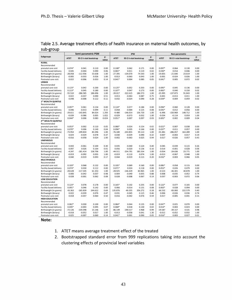
Ph.D. Thesis – Valerie Gilbert Ulep McMaster University- Health Policy
43
Table 2.5. Average treatment effects of health insurance on maternal health outcomes, by sub-group
Subgroups Semi-parametric PSM IPW Non-parametric
ATET 95 CI t-stat bootstrap p-
value ATET 95 CI t-stat bootstrap
p-value
ATET 95 CI t-stat bootstrap p-
value
RURAL Recommended prenatal care visit 0.074* 0.041 0.110 0.00 0.108* 0.062 0.171 0.00 0.097* 0.064 0.130 0.00 Facility-based delivery 0.045 -0.004 0.090 0.06 0.065* 0.011 0.119 0.02 0.030* 0.014 0.046 0.00 Birthweight (in grams) -28.058 -112.936 53.638 1.00 -27.395 -134.070 74.543 1.00 -19.835 -21.640 23.619 1.00 Birthweight (binary) -0.005 -0.033 0.026 1.00 -0.013 -0.063 0.043 1.00 -0.001 -0.024 0.026 1.00 Postnatal care visit 0.022 -0.006 0.053 0.14 0.041* 0.004 0.085 0.05 0.041* 0.005 0.072 0.02 URBAN Recommended prenatal care visit 0.123* 0.042 0.200 0.00 0.125* 0.052 0.203 0.00 0.095* 0.045 0.136 0.00 Facility-based delivery 0.113* 0.045 0.180 0.00 0.107* 0.047 0.173 0.00 0.065* 0.040 0.150 0.02 Birthweight (in grams) -55.510 -286.585 186.696 1.00 -39.017 -322.615 186.573 1.00 -25.995 -137.873 91.843 1.00 Birthweight (binary) 0.022 -0.037 0.090 0.51 0.013 -0.063 0.087 0.75 -0.001 -0.013 0.011 1.00 Postnatal care visit 0.048 -0.008 0.112 0.11 0.032 -0.024 0.090 0.28 0.034* 0.004 0.059 0.02 1st WEALTH QUINTILE Recommended
prenatal care visit 0.097* 0.061 0.134 0.00 0.124* 0.077 0.186 0.00 0.096* 0.060 0.128 0.00 Facility-based delivery 0.046 -0.013 0.099 0.11 0.058 -0.004 0.125 0.08 0.035* 0.012 0.056 0.00 Birthweight (in grams) -29.611 -143.845 84.024 1.293 -9.480 -146.014 156.720 1.00 -6.496 -150.969 148.712 1.00 Birthweight (binary) -0.039 -0.086 0.005 1.022 -0.029 -0.073 0.032 1.00 -0.034 -0.114 0.059 1.00 Postnatal care visit 0.044* 0.006 0.083 0.024 0.051* 0.007 0.097 0.03 0.005* 0.002 0.009 0.04 2nd WEALTH QUINTILE Recommended prenatal care visit 0.053* 0.002 0.110 0.05 0.080* 0.024 0.154 0.02 0.022* 0.007 0.038 0.00 Facility-based delivery 0.070* 0.006 0.140 0.04 0.096* 0.035 0.166 0.00 0.037* 0.011 0.057 0.00 Birthweight (in grams) -73.954 -199.834 83.396 1.00 -76.180 -243.855 59.113 1.00 -55.481 -286.057 163.289 1.00 Birthweight (binary) 0.024 -0.029 0.078 0.37 0.030 -0.029 0.090 0.32 0.007 -0.003 0.017 0.19 Postnatal care visit -0.016 -0.058 0.024 1.00 0.002 -0.063 0.025 0.94 0.017 -0.026 0.057 0.43 UNIPAROUS Recommended prenatal care visit 0.043 -0.061 0.100 0.30 0.035 -0.040 0.124 0.40 0.045 -0.039 0.115 0.26 Facility-based delivery 0.097 0.026 0.164 0.01 0.056 -0.020 0.136 0.16 0.014 -0.001 0.028 0.06 Birthweight (in grams) -4.247 -181.414 158.706 1.00 -44.511 -254.791 185.554 1.00 -0.054 -24.636 23.771 1.00 Birthweight (binary) -0.019 -0.092 0.055 1.00 -0.019 -0.110 0.074 1.00 -0.013 -0.067 0.048 1.00 Postnatal care visit 0.040 -0.019 0.093 0.17 0.044 -0.019 0.115 0.20 0.032* 0.003 0.066 0.05 MULTIPAROUS Recommended prenatal care visit 0.103* 0.068 0.132 0.00 0.105* 0.069 0.160 0.00 0.085* 0.058 0.115 0.00 Facility-based delivery 0.074* 0.030 0.112 0.00 0.071* 0.024 0.118 0.00 0.053* 0.026 0.079 0.00 Birthweight (in grams) -28.628 -117.335 61.353 1.00 -28.925 -146.429 83.965 1.00 -0.523 -46.301 40.878 1.00 Birthweight (binary) 0.000 -0.042 0.037 0.98 0.004 -0.040 0.055 0.88 0.008 -0.035 0.052 0.74 Postnatal care visit 0.028 -0.001 0.062 0.08 0.028 -0.008 0.067 0.14 0.037 -0.003 0.072 0.06 LOW EDUCATION Recommended prenatal care visit 0.123* 0.078 0.178 0.00 0.165* 0.102 0.255 0.00 0.122* 0.077 0.165 0.00 Facility-based delivery 0.091* 0.046 0.142 0.00 0.066 -0.014 0.131 0.08 0.063* 0.028 0.094 0.00 Birthweight (in grams) 43.363 -165.839 244.612 0.69 135.876 -40.355 356.272 0.18 66.532 -83.083 222.579 0.40 Birthweight (binary) 0.022 -0.039 0.076 0.47 0.031 -0.045 0.115 0.46 0.006 -0.026 0.036 0.74 Postnatal care visit 0.018 -0.037 0.064 0.50 0.016 -0.042 0.076 0.59 0.017 -0.005 0.041 0.15 HIGH EDUCATION Recommended prenatal care visit 0.062* 0.030 0.100 0.00 0.084* 0.044 0.135 0.00 0.047* 0.025 0.070 0.00 Facility-based delivery 0.045* -0.003 0.095 0.07 0.068* 0.018 0.130 0.02 0.014* 0.003 0.023 0.00 Birthweight (in grams) -72.126 -159.398 15.146 1.00 -86.149 -190.517 3.968 0.99 -19.587 -39.157 4.531 0.98 Birthweight (binary) -0.018 -0.052 0.017 1.00 -0.013 -0.058 0.041 1.30 -0.012 -0.052 0.032 1.00 Postnatal care visit 0.025 -0.007 0.060 0.14 0.041* 0.001 0.090 0.05 0.016* 0.003 0.027 0.01
Note:
1. ATET means average treatment effect of the treated
2. Bootstrapped standard error from 999 replications taking into account the
clustering effects of provincial level variables

Ph.D. Thesis – Valerie Gilbert Ulep McMaster University- Health Policy
44
Chapter 3: The impacts of subsidized health
insurance expansion in Indonesia on healthcare
use, health and healthcare expenditures
Ph.D. Thesis – Valerie Gilbert Ulep McMaster University- Health Policy
45
3.1. Introduction
Out-of-pocket health spending has adverse effects on healthcare access and use,
and these effects can be catastrophic for the poor. According to the World Health
Organization, in low and middle-income countries 400 million people do not have access
to basic healthcare services, and 150 million people fall into extreme poverty every year
because of healthcare-related spending. In response to these challenges, in recent years,
governments around the world have channeled more resources into the health sector in
an effort to achieve universal health coverage (UHC) (World Health Organization, 2010).
As a first step to achieve UHC, given their limited resources, a common strategy
of governments in LMICs is the expansion of health insurance for the poor and
vulnerable populations. While this falls short of the ultimate goal of UHC, which is to
ensure health insurance for all citizens regardless of socio-economic status, it allocates
resources to the population with the greatest needs (Giedion, Alfonso & Diaz, 2013).
Indonesia exemplifies this pattern. In 2005 the government introduced a public
insurance program—Askeskin—targeted at the poor. In 2007, the Indonesian
government renamed the program—to Jamkesmas—and expanded its coverage to
include both the poor and near-poor (Harimurti, Pigazzini, Pambudi & Tandon, 2013;
Mahendradhata, Trisnantoro, Listyadewi, Harimurti & Prawira, 2017). These initiatives
played a central role in increasing the national insurance coverage rate from 20% in
2000 to 50% in 2014.

Ph.D. Thesis – Valerie Gilbert Ulep McMaster University- Health Policy
46
The Indonesian government invested heavily in the Jamkesmas program, and
while the increase in the share of the population covered suggests that it was a success,
the large investment warrants a rigorous impact evaluation, which is the purpose of our
study. It is to the best of our knowledge the first to examine the impact of the
introduction and expansion of Indonesia’s subsidized health insurance from 2004 to
2014. In addition to its targeted approach, which is shared with many low and middle-
income countries, Indonesia is an interesting case to examine because of its
decentralized healthcare system. While targeting criteria are developed nationally, their
interpretation and implementation occur at the local level. This introduces variation
across local governments and admits a larger role for subjective and political
considerations in its implementation. Finally, because enrolment is not mandatory—
again, a feature shared with many other low and middle-income countries’ programs—
enrolment in Jamkesmas is subject to selection problems that can compromise both its
effectiveness and the ability to assess it.
In this study, we use a 15-year panel dataset (waves in 2000, 2007 and 2014) to
examine the impact of Jamkesmas on healthcare use, health outcomes, and catastrophic
healthcare expenditures. The long follow-up period allows us to account for its long-
term effects, especially on slow-moving conditions such as chronic illness and associated
risk factors. Importantly, our data include detailed measures of the use of healthcare
and health status, including anthropometric, biochemical and self-reported measures.
Using these different measures allow us to examine the impact of health insurance from

Ph.D. Thesis – Valerie Gilbert Ulep McMaster University- Health Policy
47
different viewpoints regarding patient health status, which is important given a multi-
dimensional concept of health.
3.2. Impact of health insurance in low and middle-income countries
General systematic reviews on the impact of insurance coverage on healthcare
demand and on health status are available elsewhere (Chollet, 2006; Ringel, Hosek,
Vollaard & Mahnovski, 2002; Zweifel & Manning, 2000). Here, we only focus on studies
conducted in low and middle-income countries.
Despite the growing number of empirical studies on the impact of health
insurance in low and middle-income countries, the impacts of health insurance
programs remain inconclusive (Giedion, Alfonso & Diaz, 2013; Lagarde & Palmer, 2011;
Spaan et al., 2012). As we describe below, the reasons for this are numerous, but a
fundamental problem is that weak study designs undermine the quality of the evidence
and what we can conclude (Giedion, Alfonso & Diaz, 2013).
These weak designs are rooted in a number of factors. First, because most health
insurance programs in low and middle-income countries are not mandatory, and
therefore prone to selection bias, a key challenge to evaluation is endogenous
participation. Second, while a few randomized controlled trials have been implemented,
they often suffer from limited external validity. Generalizability is further challenged by
the fact that the design of health insurance programs in low and middle-income
countries reflect contextual differences, particularly in terms of target population,

Ph.D. Thesis – Valerie Gilbert Ulep McMaster University- Health Policy
48
services covered, funding mechanisms, and the structure of the healthcare system (i.e.,
the role of public and private sectors in service delivery and financing). Third, most
studies are confounded by changes in the delivery system such as the introduction of
supply-side reforms in parallel with health insurance expansion, which is one of the
reasons for variation in the results across studies. Finally, variation across studies in the
(often limited) data available and in the health-related outcomes that can be studied,
further make it challenging to draw general lessons regarding the impact of health
insurance programs.
3.2.1. Impact on healthcare use
In light of the above, it is hard to make a general statement regarding the effect
of health insurance on healthcare use because the impact varies considerably across
different measures of healthcare use, population groups and context. For instance, the
impact can differ for general measures compared to specific measures of healthcare use.
General measures include consumption of non-specific healthcare services or goods,
such as healthcare facility visits or hospital admissions. Specific measures include
consumption of well-defined goods and services such as immunization, pap smear, and
hypertensive drugs. Health insurance introduced in Gansu Province, China, for example,
increased immunization rates but had no significant impact on inpatient or outpatient
care visits (Wagstaff & Yu, 2007). Johar (2009) shows that an Indonesian health
insurance program increased the consumption of contraceptives, but had no significant

Ph.D. Thesis – Valerie Gilbert Ulep McMaster University- Health Policy
49
impact on the use of preventive services. In explaining the results, Johar (2009) notes
that demand for some healthcare services and goods might be highly price inelastic.
Hence, consumption remains the same with or without health insurance. Second,
supply-side issues can sometimes explain these differences. Health insurance has a
greater impact on healthcare use under service-specific “vertical programs” focused in
services such as immunization, tuberculosis treatment, family planning, and maternal
and healthcare services because they are often better able to respond to demand
created by health insurance.
Health insurance does not always increase overall healthcare use because it can
increase the use of some services, but decrease the use of other services. The
introduction of health insurance could increase the consumption of outpatient care,
while reducing inpatient care (or vice versa). In Thailand, the insurance benefit of UC
Program Scheme was designed to increase outpatient care and decrease inpatient care
as a strategy to contain cost (Limwattananon et al., 2015; Panpiemras, Puttitanun,
Samphantharak & Thampanishvong, 2011). In contrast, health insurance programs in
Colombia and Ecuador were more focused on inpatient care benefits, which led to
higher hospitalization rates and lower outpatient care visits (Trujillo, 2003; Waters,
1999). Introduction of health insurance can also decrease the use of non-formal
healthcare services (Wang, Yip, Zhang & Hsiao, 2009) and differentially change the use
of public and private healthcare facilities (Thornton et al., 2010).

Ph.D. Thesis – Valerie Gilbert Ulep McMaster University- Health Policy
50
Lastly, the impact of health insurance also varies across socio-economic groups.
Low-income individuals, for example, are generally more sensitive to a reduction in the
price of healthcare because of health insurance. But the ultimate impact can depend on
the design of insurance programs and the availability of services among different groups
in society. One of the major factors that determine the impact among poor is the level of
copayment. Cost-sharing and low maximum coverage limits can make healthcare
unaffordable despite the availability of health insurance. Further, in some settings,
informal payments to health workers and other non-medical costs (e.g. transportation
costs) keep healthcare unaffordable even for poor with health insurance (Wagstaff,
Lindelow, Jun, Ling & Juncheng, 2009).
In summary, the expansion of insurance appears to affect use, but the precise
ways it does so depends importantly on the nature of the health insurance provided –
the services covered, rates of cost-sharing –and the nature of the delivery system.
3.2.2. Impact on health outcomes
In most jurisdictions, the ultimate goal of health insurance is to improve health.
Increased healthcare utilization and reduced out-of-pocket expenditures are the
intermediate goals. However, studies of the impact of health insurance on health
outcomes in low and middle-income countries are quite limited. This is due in part to
limited availability of appropriate outcome measures (Giedion, Alfonso & Diaz, 2013).

Ph.D. Thesis – Valerie Gilbert Ulep McMaster University- Health Policy
51
The available studies show mixed findings. Here, we identify two general issues that
make it challenging to draw a definitive conclusion.
First, studies that demonstrate significant impacts of health insurance programs
on health outcomes are often confounded by healthcare delivery reforms. Wagstaff &
Yu (2007) show that a health insurance program in China reduced the number of sick
days among the poor, but in addition to expanding health insurance, the government
simultaneously infused large capital investments for hospital infrastructure and
introduced reforms to improve the efficiency and quality of healthcare services.
Quimbo, Peabody, Shimkhada, Florentino & Solon (2011) show that subsidized health
insurance decreased the likelihood of Filipino children having infections and muscle
wasting, however, the intervention also included an information and education
campaign for mothers receiving the health insurance cards. Gertler, Giovagnoli &
Martinez (2014) show that the expansion of Plan Nacer, which extended health
insurance to Argentinian women, reduced the probability of extremely low birthweight
and infant mortality, but the program also introduced pay-for-performance programs to
local governments.
Second, studies suffer from methodological limitations. To observe the impact of
Health insurance, the outcome measure of choice should be relevant. Some outcome
measures remain unaffected even after the introduction of health insurance programs.
Cuevas & Parker (2010) do not find an impact of health insurance on obesity. They
argue that obesity, although an important factor of health is “notoriously difficult” to

Ph.D. Thesis – Valerie Gilbert Ulep McMaster University- Health Policy
52
overcome no matter how much attention is received. Also, health is multi-dimensional
in concept. Health insurance could have a different impact on subjective health and
objective health outcomes. In practice, self-rated health is commonly used to measure
health status because it is easier to collect in population surveys, while objective
measures of health are seldom collected because they require clinical measurement and
testing. The timing of measurement of health outcomes also appears to be crucial. The
impact of health insurance on chronic conditions and behavior may take some time to
have detectable changes. In some empirical studies, researchers have noted short follow
up as a potential reason for the lack of an observable impact of health insurance on
health outcomes (Chen et al., 2007; Quimbo, Peabody, Shimkhada, Florentino & Solon
(2011). For example, King et al. (2009) examine the impact of Mexico’s health insurance
program for the poor (Seguro Popular) on health outcomes using a community
experiment. The program shows effects on healthcare utilization, but not on health
outcomes. The authors argue that the lack of detectable impact on health outcomes is
possibly due to the short duration of treatment (10 months), and longer assessment
periods are needed to ascertain the long-term effects of the program.
3.3. Indonesia: general information
Indonesia is a nation of islands, with a population of 250 million, making it the
fourth most populous country in the world. The World Bank classifies Indonesia as a low
middle-income country. Like many countries in Asia, Indonesia has experienced rapid

Ph.D. Thesis – Valerie Gilbert Ulep McMaster University- Health Policy
53
economic growth in the last 15 years. The average annual economic GDP growth rate (in
constant prices) from 2000 to 2015 was 5.8%, well above the global average of 2.8%.
The GDP per capita income (in constant prices) increased from 2,143 USD in 2000 to
3,974 USD in 2015 (World Bank, 2017). Despite the rapid economic growth, poverty
remains a major challenge. Eleven percent of the population (28 million people) are still
considered poor, and a large portion of the population, known as near-poor, is
vulnerable to falling into poverty as their income is just above the national poverty line.
In 2012, the World Bank estimated that 40% of the population is considered poor or
near-poor (Aji, 2015; World Bank, 2012).
In recent years, Indonesia has made remarkable progress in improving health
outcomes. The infant mortality rate (IMR), one of the most sensitive measures of
general health status, decreased from 41 infant deaths per 1000 livebirths in 2000 to 21
infant deaths per 1000 livebirths in 2015 (World Bank, 2017), meeting Indonesia’s
Millennium Development Goal, which was to reduce IMR from 68 in 1990 to 23 by 2015
(Association of Southeast Asian Nations, 2017). Despite the improvement in health
outcomes, Indonesia still faces geographic and income-related health inequalities. For
instance, the IMR among the poorest wealth quintile is 52 compared to 17 among the
richest wealth quintile (Statistics Indonesia, 2013).
3.3.1. Indonesia: healthcare delivery system
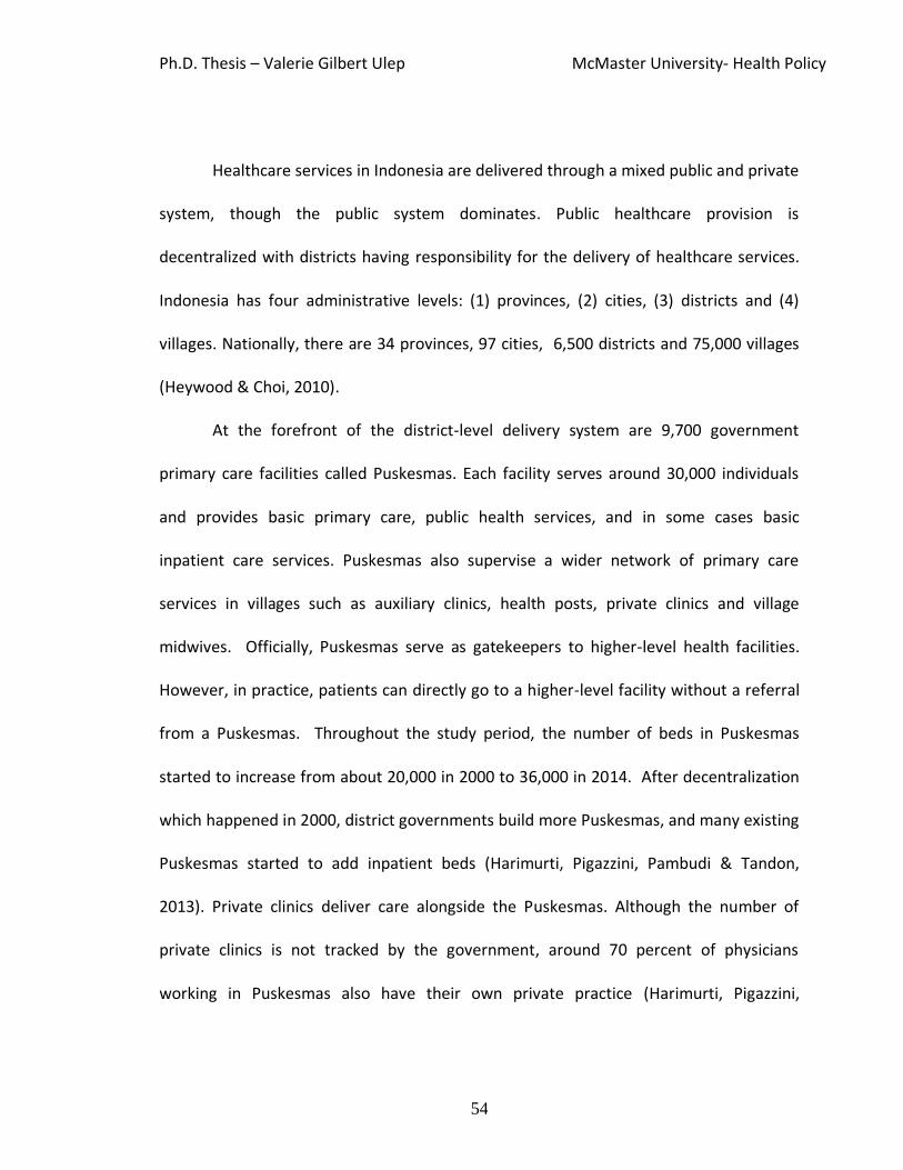
Ph.D. Thesis – Valerie Gilbert Ulep McMaster University- Health Policy
54
Healthcare services in Indonesia are delivered through a mixed public and private
system, though the public system dominates. Public healthcare provision is
decentralized with districts having responsibility for the delivery of healthcare services.
Indonesia has four administrative levels: (1) provinces, (2) cities, (3) districts and (4)
villages. Nationally, there are 34 provinces, 97 cities, 6,500 districts and 75,000 villages
(Heywood & Choi, 2010).
At the forefront of the district-level delivery system are 9,700 government
primary care facilities called Puskesmas. Each facility serves around 30,000 individuals
and provides basic primary care, public health services, and in some cases basic
inpatient care services. Puskesmas also supervise a wider network of primary care
services in villages such as auxiliary clinics, health posts, private clinics and village
midwives. Officially, Puskesmas serve as gatekeepers to higher-level health facilities.
However, in practice, patients can directly go to a higher-level facility without a referral
from a Puskesmas. Throughout the study period, the number of beds in Puskesmas
started to increase from about 20,000 in 2000 to 36,000 in 2014. After decentralization
which happened in 2000, district governments build more Puskesmas, and many existing
Puskesmas started to add inpatient beds (Harimurti, Pigazzini, Pambudi & Tandon,
2013). Private clinics deliver care alongside the Puskesmas. Although the number of
private clinics is not tracked by the government, around 70 percent of physicians
working in Puskesmas also have their own private practice (Harimurti, Pigazzini,

Ph.D. Thesis – Valerie Gilbert Ulep McMaster University- Health Policy
55
Pambudi & Tandon, 2013; Mahendradhata, Trisnantoro, Listyadewi, Harimurti &
Prawira, 2017).
Inpatient care is provided by public and private hospitals. Indonesia has 1,632
secondary hospitals, of which 50% are public, and 372 tertiary hospitals providing high-
level and specialized care, 80% of which are public. Almost all public hospitals are
controlled by district governments. Most hospitals, particularly the privately-owned
ones, are located in cities, and access to inpatient care is a major problem in many rural
areas. In the last 15 years, the number of hospitals has increased and the associated
number of inpatient beds per 1000 population increased from 0.97 in 2000 to 1.26 in
2014 (Appendix 2.1). The growth was partly because of private sector investments that
increased the number of beds in private hospitals. The use of private and public
hospitals varies by income group, with the rich tending to use private hospitals and the
poor tending to use public facilities (Harimurti, Pigazzini, Pambudi & Tandon, 2013;
Mahendradhata, Trisnantoro, Listyadewi, Harimurti & Prawira, 2017; Mahendradhata,
Trisnantoro, Listyadewi, Harimurti & Prawira, 2017). Indonesia comprises 17,000 islands,
making it hard for those living on remote islands to access healthcare services, especially
hospitals.
3.3.2. Indonesia: healthcare financing system
From 2000 to 2014, the average annual growth rate in healthcare expenditure
per capita (in constant prices) in Indonesia was 9.5% (91 USD in 2000 to 299 in 2014).

Ph.D. Thesis – Valerie Gilbert Ulep McMaster University- Health Policy
56
Over the same period, the share of health expenditure to GDP increased from 2% in
2000 to 2.8%, although this level remains relatively low compared to countries in Asia
(World Bank, 2016; Mahendradhata, Trisnantoro, Listyadewi, Harimurti & Prawira,
2017). The low share is attributed to low public spending. The share of public spending
to total healthcare expenditure remained relatively stable: 36% in 2000 and 38% in
2014. The majority of private spending (70%) was out-of-pocket payments
(Mahendradhata, Trisnantoro, Listyadewi, Harimurti & Prawira, 2017); Panpiemras et al.,
2011; Rokx, Schieber, Harimurti, Tandon & Somanathan, 2009) (Appendix 3.2).
In Indonesia, the flow of financing is complex and overlapping. District
governments directly finance public health services, capital outlays for public healthcare
facilities and salaries of healthcare workers in clinics. However, district governments
receive grants from the provincial and national governments to augment their public
health programs. Public health insurance, which included a number of distinct
programs, is financed by a mixture of national and subnational governments.
The public health insurance system includes a set of distinct health insurance
programs. Each program has its own management and source of financing, and attempts
to cover specific population groups. Jamsotek and Askes are longstanding mandatory
health insurance schemes of the national government that cover the private and public
formal sector employees. Jamkesmas is a health insurance program of the national
government that covers the poor and near-poor informal workers. In 2007, some local
governments also introduced a health insurance program called Jamkesda, which covers

Ph.D. Thesis – Valerie Gilbert Ulep McMaster University- Health Policy
57
poor households that are not captured by Jamkesmas program due to mistargeting, and,
in some districts, it supplements Jamkesmas. The introduction of Jamkesda in parallel
with Jamkesmas is regarded as politically motivated. Jamkesda has provided some local
governments the opportunity to use “free healthcare services” as a popular campaign
tagline (Dwicaksono, Nurman & Prasetya, 2012). In 2011, the national government also
introduced Jampersal, a health insurance program for poor mothers not covered by
Jamkesmas, again because of mistargeting. Because Jamkesmas failed to cover a
significant number of poor mothers, Jampersal is an effort to reduce maternal and infant
deaths through a scheme solely devoted to identifying and enrolling poor mothers, and
covering only maternal and child-related services (Achadi, Achadi, Pambudi & Marzoeki,
2014).
In addition to public health insurance programs, there are private sources of
financing such as private health insurance and savings-related insurance. However, only
a small portion of the population is covered by private health insurance plans (usually
the rich). Table 3.1 shows the different coverage rates by income tercile of different
health insurance programs in Indonesia for the period 2000 to 2014. Pro-poor health
insurance programs such as Jamkesmas, Jamkesda, and Jampersal are seemingly
mistargeted since a meaningful portion of the rich population is covered by these
targeted health insurance programs.
3.3.3. Description of Jamkesmas

Ph.D. Thesis – Valerie Gilbert Ulep McMaster University- Health Policy
58
Jamkesmas is the primary government health insurance program targeted at
poor (those below the poverty line) and near-poor (those just above the poverty line
and at risk of falling into poverty) informal workers. Originally introduced as Askeksin in
2005 and targeted at only the poor, in 2007, it was renamed as Jamkesmas and was
expanded to cover the near-poor as well. Although the expansion started in 2007, large
enrollment increases only occurred in the succeeding years. In 2011, the Indonesian
government estimated 76.4 million (out of 240 million) individuals were considered poor
or near-poor and were eligible beneficiaries of Jamkesmas. Harimurti, Pigazzini, Pambudi
& Tandon (2013) estimated that 40% of the poor and near-poor were covered by the
program in 2012.While the national government facilitates the identification of eligible
beneficiaries, the districts determine eligibility and enroll beneficiaries. In 2004 and
2011, Statistics Indonesia (BPS) conducted a national poverty survey. It provided the
number of poor and near-poor for each district. Districts then validated the data from
Statistics Indonesia using their own methods. As a consequence, the specific definition
of poor and near-poor used for means testing and local government eligibility criteria
varied by district. If the number of poor and near-poor was greater than the BPS district
allocation numbers, these individuals were encouraged to enroll in other local
government health insurance programs such as Jamkesda (Harimurti, Pigazzini, Pambudi
& Tandon, 2013).
The Jamkesmas insurance premium is fully subsidized by the government, but
enrolment is not mandatory. Beneficiaries hold a Jamkesmas insurance card making

Ph.D. Thesis – Valerie Gilbert Ulep McMaster University- Health Policy
59
them eligible to receive services under the program. Some individuals opt not to be
enrolled because of stigma as bearers of Jamkesmas cards, since having the card signals
the socio-economic status of the individual. Others do not enroll because of the
administrative and bureaucratic hurdles in claiming benefits. One of the issues with
enrollment is the discretion of the enroller. In practice, the enroller has flexibility, and
the targeting criteria are partially subjective (Harimurti, Pigazzini, Pambudi & Tandon,
2013; Simmonds & Hort, 2013; Suryahadi, Febriany & Yumna, 2014). One-fifth (21%) of
all Jamkesmas holders belonged to the top three economic deciles (Harimurti, Pigazzini,
Pambudi & Tandon, 2013). We estimate from the 2014 Indonesia Family Life Survey
(IFLS) approximately 25% of the richest income decile was enrolled in Jamkesmas, and
approximately 45% of the poorest income decile was enrolled in Jamkesmas, indicating
low uptake among the poor and evidence of mistargeting (Appendix 3.3).
The Ministry of Health at the national level defines the benefits package, which is
meant to be comprehensive. The benefits include outpatient and inpatient care in public
healthcare facilities and enlisted private healthcare facilities. On paper, all inpatient and
outpatient care services are covered except for the following: general check-ups,
cosmetic services, traditional medicines, fertility programs and dental services. Generic
versions of prescription drugs are also included as long they are on the formulary. The
MOH reimburses primary care facilities using fee-for-service and reimburses private and
public hospitals using case rates. The program does not require cost-sharing at the point
of service. However, in practice, informal payments exist and are rampant. They can

Ph.D. Thesis – Valerie Gilbert Ulep McMaster University- Health Policy
60
take different forms such as payments to health providers to cut waiting time or to
acquire additional services in healthcare facilities. They also include direct payments by
patients to health providers for certain drugs or medical services that are not in
healthcare facilities. The actual amount of informal payments is hard to estimate
(Ministry of Health, 2014).
3.4. Conceptual framework
Levy & Meltzer (2001) provide a useful conceptualization of the inter-
relationships of health insurance, healthcare utilization and health status, reproduced
below as Figure 3.1. Health depends not only on healthcare, but also on many factors
such as health behaviors, observable characteristics such as age, sex, education, income,
and unobservable characteristics such as genetic endowment and beliefs. In the case of
Jamkesmas, where participation is non-random, some of these factors (e.g. income and
education) are also likely correlated with health insurance coverage. The health status
of an individual also affects the consumption of healthcare; individuals who are
unhealthy are far more likely to seek care. In this framework, factors that affect health
insurance, healthcare and health can be observed (e.g., education, income or sex) or
unobserved (e.g., genetic endowment, belief system).
The relationship between healthcare and health in Figure 3.1 does not fully
differentiate the concept of disease, health and function. It is useful however, to
distinguish the difference between the two concepts: Evans & Stoddart (1990) define

Ph.D. Thesis – Valerie Gilbert Ulep McMaster University- Health Policy
61
“disease” as an abnormal physiologic function, and “health and function” as the
experience of the disease by an individual. In the early stages, many diseases (e.g.,
elevated blood pressure or insufficient hemoglobin) are asymptomatic and have yet to
be translated to detectable changes in health and function (e.g., self-rated health,
unproductive work days). Our outcome measures include indicators of both disease and
health and function.
3.5. Data
We use the longitudinal individual component of the Indonesian Family Life
Survey (IFLS) conducted by the RAND Corporation. IFLS is an on-going longitudinal socio-
economic and health survey. Some provinces were not surveyed because of limited
resources and it was unsafe for interviewers to go to some provinces. The survey
represents 13 of the 34 provinces, and 83% of the population. The survey collects data
on individual respondents, their families, their households, and the communities in
which they live. The first wave was administered in 1993 to 7,224 households (Strauss,
Witoelar & Bondan, 2016), and succeeding waves were conducted in 1997, 2000, 2007
and 2014. IFLS is a dynamic panel. New family or household members are interviewed
and tracked in the succeeding waves. Household or family members who appear in a
previous cohort, but who move to another place or household were tracked and
interviewed.

Ph.D. Thesis – Valerie Gilbert Ulep McMaster University- Health Policy
62
We use the 2000, 2007 and 2014 cycles of IFLS in the analysis. We link 30,815
adults (15 years old and above) in the 2000 wave with the 2007 wave. Defining non-
response to include baseline respondents who could not be located during the follow-up
survey, who died, or who were found but completely declined to participate, the non-
response rate between 2000 and 2007 was 25% (n= 7,693), of whom 6% (n= 1,930) were
reported to have died. We delete non-response between 2000 and 2007 (n=7,693), then
linked the remaining individuals to the 2014 wave. The non-response rate between 2007
and 2014 was 22% (n=5,019), of whom 7% (n=1,696) were reported to have died. Finally,
we delete non-response between 2007 and 2014 (n=5,019). The overall attrition is 41%
(7,693+5,091=12,717). At this stage, respondents who did not respond to a subset of
specific questions are still included (see Appendix 3.4 for details).
Table 3.2 shows the baseline characteristics (the year 2000) of respondents in
the sample. Excluding those who died, those lost to follow-up in either 2007 or 2014 are
more likely to be rich, a university graduate, male, and living in urban areas (see
Appendix 3.5 for the complete results of the logistic regression model). We found no
significant association between enrolment in Jamkesmas and mortality (see Appendix
3.6 for the complete results of the regression model).
3.6. Dependent Variables
We use various measures of healthcare use, health outcomes and out-of-pocket
healthcare expenditures to examine the impact of Jamkesmas.

Ph.D. Thesis – Valerie Gilbert Ulep McMaster University- Health Policy
63
3.6.1. Healthcare use
Measures of healthcare use include use of inpatient care, number of inpatient
days, use of outpatient care, and number of outpatient care visits. We also examine non-
formal healthcare use: self-medication and traditional medicine. The inpatient care
variable is a dummy variable equal to 1 if an individual was admitted to a hospital in the
12 months prior to the survey, and equal to 0 otherwise. The number of inpatient days
(conditional on having been admitted) during the most recent admission is a count
variable. The outpatient care variable is a dummy variable equal to 1 if an individual
visited an outpatient health facility in the 4 weeks prior to the survey, and equal to 0
otherwise. The number of times visited a healthcare facility for outpatient care
(conditional on having at least one visit) in the 4 weeks prior to the survey is a count
variable. We focus only on needed care (treatment to illness and injury and
consultation) and exclude visits for massage and cosmetic services. The self-medication
variable is a dummy variable equal to 1 if an individual engaged in self-medication using
a modern medicine in the 6 weeks prior to the survey, and is equal to 0 otherwise. The
traditional medicine variable is a dummy variable equal to 1 if an individual used herbal
medicine or visited a traditional healer in the 6 weeks prior to the survey, and is equal to
0 otherwise.
3.6.2. Health outcomes

Ph.D. Thesis – Valerie Gilbert Ulep McMaster University- Health Policy
64
As noted, following Evans & Stoddart (1990), we differentiate disease, health,
and function. The measures of disease were based on the anthropometric, biochemical
and clinical components of the survey for which healthcare workers collected blood
samples and performed anthropometric and clinical testing. The measures of disease
include systolic blood pressure (mmHg), hemoglobin (mg/dl), lung capacity (liter/min)
and Body Mass Index (kg/m2). Variables are specified both as continuous (in the
conventional units) and as categorical variables. High blood pressure is equal to 1 if
systolic blood pressure is more than 120 mmHg, and is otherwise 0. The variable for
anemia is equal to 1 if hemoglobin is less than 12 mg per dl and is otherwise 0. BMI is
usually classified into four categories: underweight (<18.5), normal (18.5 – 24.9),
overweight (25.0 – 29.9) and obese (>30). In this study, we re-categorize the variable
into a dummy equal to 1 if BMI is underweight and equal to 0 otherwise. We choose to
model underweight because it is more prevalent than obesity among the poor in
Indonesia. Also, we re-categorize BMI into a dummy to avoid complexity in modeling
ordinal dependent variable with fixed effects.
We select blood pressure, anemia, lung capacity and underweight as measures of
disease because they are known to affect long-term health and function. High blood
pressure is a major risk factor for ischemic heart disease and stroke, which are
associated with chronic disability and mortality. Anemia is a condition in which there
are not enough red blood cells to carry oxygen to tissues. Several infectious and chronic
conditions can cause anemia. Persistent anemia can lead to physical weakness and

Ph.D. Thesis – Valerie Gilbert Ulep McMaster University- Health Policy
65
cognitive impairment due to lack of iron. Lung capacity as measured by Peak Expiratory
Flow (PEF) indicates obstructions in the respiratory pathway caused by chronic and
acute conditions such as Chronic Obstructive Pulmonary Disease (COPD), asthma,
respiratory infection, and malnutrition. A poor cardio-pulmonary function can severely
affect physical performance and activity. Underweight could severely affect physical
function and mental health (e.g., depression).
We use two measures of health and function: self-rated health and number of
missed days of primary daily activities in a month because of illness. For the former,
individuals subjectively assess their health using four ordinal categories (i.e., healthy,
somewhat healthy, somewhat unhealthy and unhealthy). Like BMI, we re-categorize
self-rated health into a dummy equal to 1 if ‘healthy’ and ‘somewhat healthy’, otherwise
0, again to reduce the complexity in modeling an ordinal variable with fixed effects. For
the latter, individuals should report the number of days missed because of illness in the
past month (range: 0 to 30 days). Our data do not contain questions to determine their
daily activities, but it should pertain to a wide range of activities including school
attendance or employment (e.g., farming, fishing, construction, household keeping).
3.6.3. Healthcare expenditures and financial protection
The survey includes information on out-of-pocket spending incurred during the
last hospital admission and last outpatient care visit. Therefore, our measure of
healthcare expenditure is the actual out-of-pocket spending (adjusted to 2010 prices)
Ph.D. Thesis – Valerie Gilbert Ulep McMaster University- Health Policy
66
incurred during the most recent hospital admission in the last 12 months prior to the
survey, and the most recent outpatient care visit in the 4 weeks prior to the survey. For
the measure of financial protection, we follow the World Bank and World Health
Organization’s definition of catastrophic healthcare expenditure. We create a dummy
variable equal to 1 if the out-of-pocket healthcare expenditures during the last
admission exceeded 10% of household expenditure per capita per year3, equal to 0
otherwise.
3.7. Empirical strategy
3.7.1. Modelling healthcare use and healthcare expenditures
In modeling healthcare use and out-of-pocket healthcare expenditures, we use a
two-part model within a generalized linear model framework. A two-part model allows
us to model the two processes of healthcare use and healthcare spending. The first part
of a two-part model predicts whether or not an individual used healthcare or reported a
healthcare expenditure due to the last outpatient care or admission. The response
variable for the first part is binary. The second part of a two-part model predicts the
intensity of healthcare use and the actual expenditures conditional on healthcare use.
Modeling the second part is challenging because observations are not normally
distributed. Intensity and expenditure variables usually have restricted range and are
3 Household expenditure is the sum of food and non-food expenditures in a given year. In IFLS, depending on the expenditure item, the recall period varies from week to year. RAND Corporation annualized all the expenditures, but not seasonally-adjusted.

Ph.D. Thesis – Valerie Gilbert Ulep McMaster University- Health Policy
67
highly skewed, which makes OLS estimation biased and efficient. One can address the
skewed distribution using generalized linear models (GLM) (Manning, Basu & Mullahy,
2005; Manning & Mullahy, 2001), and we use these (GLM) with pooled data to predict
the intensity of healthcare use and out-of-pocket healthcare expenditures. Within the
GLM framework, we need to specify the mean and variance functions. Following Jones,
(2010) and Buntin & Zaslavsky (2003), we specify log link function in modeling for the
expected mean, which is the commonly chosen link function in healthcare utilization and
expenditure applications. In specifying the variance function, we use Modified Park’s
test, and gamma distribution seems to be the most appropriate function (Appendix 3.8).
We use the following specification for Parts 1 and 2:
Part 1: linear probability model
𝐸(𝑌𝑖𝑡|𝑋) = 𝛽0 + 𝛽1𝐽𝑎𝑚𝑘𝑒𝑠𝑚𝑎𝑠𝑖𝑡 + 𝛽2𝑂𝑡ℎ𝑒𝑟𝐼𝑛𝑠𝑢𝑟𝑎𝑛𝑐𝑒𝑖𝑡 + 𝛽3𝑌𝑒𝑎𝑟𝑠𝑀𝑒𝑚𝑏𝑒𝑟𝑖𝑡 +
𝛽4(𝑌𝑒𝑎𝑟𝑠𝑀𝑒𝑚𝑏𝑒𝑟𝑖𝑡𝑥 𝑌𝑒𝑎𝑟𝑠𝑀𝑒𝑚𝑏𝑒𝑟𝑖𝑡) + 𝐼𝑛𝑑𝑖 + 𝐷𝑖𝑠𝑡𝑟𝑖𝑐𝑡𝑖 + 𝛽5𝑋𝑖𝑡 (Equation 1)
Part 2: GLM log link function
log (𝐸(𝑌𝑖|𝑋)) = 𝛼0 + 𝛼1𝐽𝑎𝑚𝑘𝑒𝑠𝑚𝑎𝑠𝑖 + 𝑎2𝑂𝑡ℎ𝑒𝑟𝐼𝑛𝑠𝑢𝑟𝑎𝑛𝑐𝑒𝑖 + 𝑎3𝑌𝑒𝑎𝑟𝑠𝑀𝑒𝑚𝑏𝑒𝑟𝑖 +
𝛼4(𝑌𝑒𝑎𝑟𝑠𝑀𝑒𝑚𝑏𝑒𝑟𝑖𝑥 𝑌𝑒𝑎𝑟𝑠𝑀𝑒𝑚𝑏𝑒𝑟𝑖 + 𝐷𝑖𝑠𝑡𝑟𝑖𝑐𝑡𝑖 + 𝛼5𝑋𝑖 (Equation 2)
In part 1, we use a panel fixed-effects (FE) model to estimate the marginal effects
of Jamkesmas on positive use of healthcare utilization and positive out-of-pocket

Ph.D. Thesis – Valerie Gilbert Ulep McMaster University- Health Policy
68
healthcare expenditures. 𝑌𝑖𝑡 is the dichotomous outcome of interest for individual i (𝑖
=1…n) at time t (t = 1, 2, 3). We model the following outcome of interests: visited an
outpatient healthcare facility in the last 4 weeks, admitted in a hospital in the last 12
months, and incurred positive out-of-pocket healthcare expenditures due to outpatient
care or inpatient care. 𝐽𝑎𝑚𝑘𝑒𝑠𝑚𝑎𝑠𝑖𝑡 is a dummy variable that indicates whether i
individual at time t is enrolled in Jamkesmas. Because individuals could be enrolled in
multiple insurance programs, 𝑂𝑡ℎ𝑒𝑟𝐼𝑛𝑠𝑢𝑟𝑎𝑛𝑐𝑒𝑖𝑡 indicates membership in public or
private health insurance other than Jamkesmas. 𝑌𝑒𝑎𝑟𝑠𝑀𝑒𝑚𝑏𝑒𝑟𝑖𝑡 is the number of
years an individual has been enrolled in Jamkesmas. 𝐼𝑛𝑑𝑖 is the individual FE. 𝐷𝑖𝑠𝑡𝑟𝑖𝑐𝑡𝑖
is the district FE. We include individual FE to control for unobserved individual
heterogeneity. To produce an unbiased estimate, the identification assumption in a FE
model is that there is no correlation between the error and Jamkesmas because all the
relevant unobservables are “absorbed” by the FE. We include the following time-varying
covariates (𝑋𝑖𝑡): age, marital status, education, log per capita household expenditure,
employment, urbanity and survey cycle. For part 2, in addition to these variables, we
include the following health outcomes in the model: high blood pressure, lung capacity,
anemia, abnormal BMI, and self-rated health status.
We use linear probability models (OLS) in estimating the marginal effects
because it is convenient and computationally tractable. Also, the results of linear
probability model are easier to interpret, which is one key advantage of linear
probability models over logit probability models. One disadvantage of linear probability

Ph.D. Thesis – Valerie Gilbert Ulep McMaster University- Health Policy
69
models, however, is they impose heteroscedasticity in the case of a dummy variable. We
address this problem by using heteroscedasticity-consistent robust standard error
estimates. For comparison, we run logit probability models, and we observe similar
results (Appendix 3.7).
In parts 1 and 2, we run five models for each outcome of interest to see the
changes in marginal effects as we include covariates in the model. In the first model, we
only control for socio-demographic covariates. In the second model, we control health-
related variables including risky behaviors (e.g. smoking) in addition to socio-
demographic variables. In the third model, we use the same set of covariates in the
second model, but we also include duration (in years) of membership in Jamkesmas up
to second-degree polynomials. We highlight the results of the third model because in
this model we have potentially controlled not only for socio-demographic
characteristics, but also health variables, and possible temporal effects of Jamkesmas
membership. The fourth and fifth models are similar to the third model, but we stratify
the sample by poor (first tercile) and non-poor (second and third income tercile). Income
group is based on household consumption per capita at baseline.
We model the use of non-formal healthcare, self-medication, and use of
traditional medicine, for which we have only a measure of whether there was any use
(no intensity of use). We specify the model using equation 1.
3.7.2. Modelling health outcomes

Ph.D. Thesis – Valerie Gilbert Ulep McMaster University- Health Policy
70
Modelling health outcomes
We use a panel FE OLS model to examine the impact of Jamkesmas on the
following health outcomes: systolic blood pressure (continuous), lung capacity
(continuous), anemia (binary), hypertension (binary) and underweight (binary). For the
number of missed primary daily activities in the last month, a count variable, we use a
negative binomial FE model. In specifying the model, we include the following time-
varying covariates: years of membership in Jamkesmas, age, marital status, education,
log per capita household expenditure, employment, urbanity, survey cycle, and
comorbidities. We also include district fixed effects. We run five models for each
outcome of interest to see how the incremental inclusion of additional covariates
changes the estimated impact of Jamkesmas on health outcomes.
3.8. Results
Table 3.2 presents the characteristics of the respondents at baseline. Of the 18,
103, fifty-four percent are males, approximately 40% had grade school as the highest
level of attainment, 30% were formal sector workers, 70% were married, and 65% were
smokers. The distribution of respondents living in urban and rural areas was
approximately the same. Table 3.3 presents the distribution of dependent variable:
healthcare use, health outcomes and out-of-pocket healthcare expenditures of
respondents by survey wave. Among healthcare utilization variables, we observe a
monotonic upward trend over time only for inpatient care. The percentage of

Ph.D. Thesis – Valerie Gilbert Ulep McMaster University- Health Policy
71
respondents who had inpatient care increased from 2.0% in 2000 to 5.0% in 2014.
Although the percentage of respondents who had inpatient care increased, the average
inpatient days during the last admission remained the same. Unlike inpatient care,
outpatient care visits decreased over the period. The percentage of respondents with
outpatient care visits decreased from 11% in 2000 to 6.0% in 2007, then slightly
increased to 8.0% in 2014. However, we observe no change in the average number of
outpatient care visits, conditional on having at least one visit.
We observe a SES-gradient in the share of respondents with inpatient and
outpatient care. The rich are more likely to have outpatient and inpatient care than the
poor, a consistent pattern in all three survey periods. However, there is no noticeable
SES-gradient in the number of inpatient days conditional on having been admitted or the
number of visits to a healthcare facility for outpatient care conditional on having at least
one visit. Nor is there a consistent SES-gradient for non-formal healthcare use in three
survey periods.
The prevalence of hypertension shows an upward trend, while the prevalence of
underweight shows a downward trend. The prevalence of hypertension increased from
49.0% in 2000 to 73.0% in 2014, while the prevalence of underweight decreased from
17.3% in 2000 to 9.8% in 2014. Self-rated health shows an interesting pattern. The
percentage of respondents who rated themselves ‘healthy’ (category 1) increased from
8.2% in 2000 to 16.6% in 2014. This is a large increase. At the same time, the share of
respondents who considered themselves ‘somewhat healthy’ decreased (category 2),

Ph.D. Thesis – Valerie Gilbert Ulep McMaster University- Health Policy
72
and the share of respondents who considered themselves ‘somewhat unhealthy’ and
‘unhealthy’ increased. The survey question on self-rated health did not change in the
three surveys waves so we investigated this movement of responses across the four
categories. Among those who reported to be ‘somewhat healthy’ in 2007 (n=2,198), 8%
moved up to ‘healthy’, 39% remained ‘somewhat healthy’, 69% moved down to
‘somewhat unhealthy,’ and no one moved down to ‘unhealthy’ category in 2014.
Stratifying by age group, among those who reported to be ‘somewhat healthy’ in 2007
and shifted to ‘healthy’ in 2014 were more likely from younger age groups, and those
who shifted from ‘somewhat healthy’ in 2007 to ‘somewhat unhealthy’ were from older
age groups (see Appendix 3.9 for the transition matrix by age group). The prevalence of
underweight was higher among the poor, and the prevalence of obesity was higher
among the rich, a consistent pattern in all survey waves
The average out-of-pocket healthcare expenditures (in 2010 prices) during last
visit increase over time. In contrast, out-of-pocket expenditures due to inpatient care
during last admission did not follow a monotonic trend. It increased from 2000 to 2007,
then decreased in 2014. The rich have higher out-of-pocket healthcare expenditures
compared to the poor, and the income gradient was consistent in all survey periods.
The share of respondents with catastrophic healthcare expenditures was consistent over
time, but the rich tend to have a higher share, a consistent pattern found in developing
countries.

Ph.D. Thesis – Valerie Gilbert Ulep McMaster University- Health Policy
73
Table 3.4 shows the descriptive statistics of dependent variables by Jamkesmas
membership for 2007 or 2014 as well as information from 2000 before the introduction
of Jamkesmas, and Table 3.5 does the same for the independent control variables. The
first and second columns of Tables 3.4 and 3.5 show the descriptive statistics of all
dependent and independent variables at baseline (2000) by future Jamkesmas
membership status in 2007 or 2014. The distribution of dependent variables at baseline
shows small differences between future Jamkesmas and non-Jamkesmas members.
However, over time, the difference between members and non-members widened for
use of outpatient care, use of inpatient care and use of self-medication.
There is some indication that Jamkesmas members were less healthy. At
baseline, future Jamkesmas and non-Jamkesmas members have lower lung capacity,
were underweight and had lower self-rated health compared to non-members.
However, the differences were small and not clinically important. We did not observe
any large changes in the difference between members and non-members over time in
any of the health outcomes except for the number of missed days of primary daily
activities because of illness. The average OOP healthcare expenditures due to
outpatient care and inpatient care were slightly different for future Jamkesmas and non-
Jamkesmas members, a difference that widened over time. However, we did not
observe large changes in the difference between catastrophic healthcare expenditure.
In summary, we did not observe a meaningful difference in the mean values of
the dependent variables by future Jamkesmas and non-Jamkesmas membership.

Ph.D. Thesis – Valerie Gilbert Ulep McMaster University- Health Policy
74
Table 3.5 shows the descriptive statistics for the independent variables by
Jamkesmas membership and survey period. At baseline, future Jamkesmas members
were more likely to have lower education, be poor and self-employed. Jamkesmas
targets poor and near-poor workers in the informal sector so systematic differences in
terms of education, income group and employment between Jamkesmas members and
non-members are expected. However, the difference in the distribution by Jamkesmas
membership widened over time in some independent variables such as employment and
income, but the difference for other variables remained relatively the same.
Regression results: outpatient and inpatient care
Table 3.6 shows the marginal effects of Jamkesmas on healthcare use from our
two-part model. Focusing first on outpatient care, we find an association between
Jamkesmas with higher likelihood of having an outpatient care even after controlling for
covariates including years of membership (Model 3; 𝛽1 = 0.023). If we stratify the
model by income group, the marginal effects are not statistically significant (Models 4
and 5; 𝛽1′𝑠). Also, the duration of Jamkesmas membership is not associated with the
likelihood of having an outpatient care (Model 1-5; 𝛽3, 𝛽4). The results for the part-2
GLM model indicate that although we observe higher likelihood of having an outpatient
care, Jamkesmas is not associated with the frequency of outpatient care among those
with at least one visit after controlling for years of membership (Model 3; 𝑎1). Although,

Ph.D. Thesis – Valerie Gilbert Ulep McMaster University- Health Policy
75
we find statistically significant marginal effects if we exclude years of membership as
one of the covariates (Models 1 and 2; 𝑎3, 𝑎4).
Jamkesmas is associated with higher likelihood of having an inpatient care. The
marginal effects are statistically significant in Models 1 to 3, and we observe a large
marginal effect in Model 3 (𝛽1=0.032). Interestingly, we observe heterogeneity of
marginal effects between poor and non-poor. We find large and statistically significant
marginal effects among the non-poor (Model 4; 𝛽1=0.042), but insignificant among the
poor. The duration of Jamkesmas membership is not associated with the likelihood of
inpatient care (Model 1-5; 𝛽3, 𝛽4). The results for the part-2 GLM model suggests that
Jamkesmas is not associated with duration of inpatient days (Model 3; 𝑎1).
Jamkesmas is not associated with the use of self-medication and traditional
medicine after controlling for covariates including years of membership (Model 3; 𝛽3 ).
However, we find positive marginal effects on self-medication if we exclude years of
membership as one of the covariates (Model 1-2; 𝛽3, 𝛽4). We find no impact on the use
traditional medicine in all models.
Regression results: health outcomes
Tables 3.7a and 3.7b show the marginal effects of Jamkesmas on our measures
of health outcomes. In Models 1 and 2 (𝛽1), the marginal effects of Jamkesmas on
systolic blood pressure and lung capacity (continuous) are significant, though the
statistical significance disappears in Model 3 (𝛽1). We did not observe any significant
Ph.D. Thesis – Valerie Gilbert Ulep McMaster University- Health Policy
76
impact for hypertension (binary), anemia (binary), underweight (binary), and self-rated
health (binary) in any model. To validate our estimates for underweight, we also ran a
pooled ordinal logit using BMI with four categories, and found no statistically significant
marginal effects (data not shown). The marginal effects for the duration of Jamkesmas
membership are not statistically significant for any of the health outcome measures in
all models (𝛽3, 𝛽4).
The marginal effects of Jamkemas on the number of missed days of primary daily
activities are statistically significant in Models 1 to 3, with Model 3 having the largest
marginal effects ((𝛽1, =0.204). When we stratify the model by income, we observe large
marginal effects among the poor (𝛽3, =0.312 days). and a non-statistically significant
effect among the non-poor (Model 5).
Regression results: OOP and financial protection
Table 3.8 shows the marginal effects of Jamkesmas on OOP and catastrophic
healthcare expenditures. Jamkesmas is associated with lower OOP incurred during the
last outpatient care and inpatient care in Models 1 and 2, but the effect decreases in
magnitude and becomes statistically non-significant when we include the full set of
covariates in Model 3. We observe a similar pattern for OOP incurred during the last
admission. The marginal effects are statistically significant in Models 1 and 2, but not
significant in Model 3, with decreasing marginal effects as we include more covariates.
When we stratify the model by income group, the marginal effects of Jamkesmas on

Ph.D. Thesis – Valerie Gilbert Ulep McMaster University- Health Policy
77
OOP incurred during outpatient or inpatient care are larger among the poor. We find no
evidence that Jamkesmas is associated with lower catastrophic healthcare expenditures.
3.9. Discussion
In this study, we investigated the impact of the expansion of Jamkesmas, a public
insurance program targeted at the poor and non-poor in Indonesia, on healthcare
utilization, health outcomes, and out-of-pocket healthcare expenditures. Jamkesmas is
the largest subsidized health insurance program in Indonesia. Although the program
targets the poor and near-poor population, we observed leakage, with a significant
portion of the Jamkesmas members being non-poor. Also, the program suffered from
low uptake. In 2014, only about 50% of the poorest decile were enrolled in the
program. Mistargeting is a problem shared by many subsidized health insurance
programs in low and middle-income countries. This problem opens important policy
questions about whether Jamkesmas is meeting its pro-poor objective.
One challenge in examining the causal impact of Jamkesmas is selection. As
discussed earlier, enrollment is voluntary and subject to some discretion by program
staff, resulting in non-random participation. Jamkesmas participation may be associated
with individual and district level-characteristics. However, the problem of selection in
this case does not appear to be large, at least on observables. The typical selection
problem in voluntary health insurance participation is that members are systematically

Ph.D. Thesis – Valerie Gilbert Ulep McMaster University- Health Policy
78
different from non-members. In the case of Jamkesmas, although the differences
between members and non-members for some health outcomes are statistically
significant, the differences are small and clinically unimportant. We only observed large
differences in income, education, and employment, which is expected given the
targeted nature of the program. This still leaves the possibility of selection on
unobservables. To the extent that such selection was based on invariant unobserved
effects, our use of fixed-effects models where possible can correct for such a problem.
During the period of our study, Indonesia experienced a significant supply-side
reform. As noted in our literature review, the number of government clinics (Puskesmas)
started to increase after decentralization in 2000. The increase in supply-side that
occurred in the last 15 years could have affected healthcare use with or without health
insurance. However, the impact of supply-side reforms may be considered random as it
affects both treatment and comparison group hence it should not bias our estimates.
Our findings suggest that Jamkesmas is associated with a higher probability of
having outpatient care. Our study also explored the intensity of healthcare use, which is
often not examined in empirical studies in low and middle-income countries because
such information is seldom collected. We found that Jamkesmas increases the frequency
of outpatient care. It is also associated with a higher probability of having inpatient care,
with a larger impact among the non-poor, but no significant impact on the number of
inpatient days during the most recent inpatient visit. This makes Jamkesmas a subsidized

Ph.D. Thesis – Valerie Gilbert Ulep McMaster University- Health Policy
79
health insurance program in a low and middle-income country with a positive impact on
healthcare use, and in particular a positive impact on both inpatient and outpatient care.
The positive impact of Jamkesmas on outpatient care is promising. The goal of a
health system is to expand outpatient care, particularly preventive, rather than inpatient
care and especially to population groups who are at more risk of serious conditions.
However, the positive impact of Jamkemas on inpatient care among the non-poor, and
the lack of impact among the poor is striking. If the benefits of an insurance program are
not accruing for the intended beneficiaries, this may be evidence of poor targeting. This
finding points to the seemingly pro-rich effects of a pro-poor program like Jamkesmas
when there is weak targeting and aspects of the delivery system favor the rich. It is
possible that this finding is a reflection of the differential access to inpatient care of poor
and non-poor other than health insurance.
In general, Jamkesmas is not associated with improvements in any health
outcomes even after controlling for temporal effects. The median duration of
membership is approximately 2 years, and longer duration may be needed to detect
changes, especially for chronic conditions.
There are several possible explanations for why Jamkemas improved healthcare
use but did not produce improvements in health. First, health insurance can increase
healthcare use, but healthcare services may not be a major determinant of health status
(Chen et al., 2007; Smith, 1999). The social determinants of health framework suggests
that health is determined not only by healthcare but by physical, environmental and
Ph.D. Thesis – Valerie Gilbert Ulep McMaster University- Health Policy
80
other socio-economic conditions (Smith, 1999; Evans & Stoddart, 1990). Second, the lack
of observable impact might be a reflection of the poor quality of healthcare services. In
low-resource settings, quantity is often prioritized over quality. Third, the increase in
healthcare use might be attributed to an increase in the use of marginally effective
services with small associated health benefits (Chen et al., 2007).
Although we found no evidence of an impact on health outcomes, our findings
show a significantly higher number of missed days of daily activities reported by
Jamkemas members, and the marginal effects are more pronounced among the poor.
Initially, we hypothesized that health insurance would reduce the number of reported
missed days of daily primary activity last month. However, our findings say otherwise.
Because ‘daily primary activity’ is a broad concept, it is hard to make a general
conclusion. In the case of informal workers who have health insurance, members who
are sick may have now have access to healthcare providers who will advise them to stop
working and rest to aid recovery. To our knowledge, no study has used this outcome
before hence our findings provide a new insight, which is worth exploring in future
research especially in other contexts.
Jamkesmas is associated with lower out-of-pocket healthcare expenditures, and
the poor seem to have benefitted more. However, we did not find evidence that
Jamkesmas is associated with lower catastrophic healthcare expenditures, meaning,
although OOP significantly decreased, it was not large enough to make a significant
reduction in the contribution of OOP relative to one’s total expenditure or income. This

Ph.D. Thesis – Valerie Gilbert Ulep McMaster University- Health Policy
81
finding is also observed in other empirical studies especially in programs with
unregulated copayments (Wagstaff, Lindelow, Jun, Ling & Juncheng, 2009).
There are numbers of limitations in the expenditure data of IFLS that might affect
the validity of our results. First, we only evaluated the OOP health expenditure during
the last admission in the past 12 months hence we might have not fully evaluated the
effects of health insurance on catastrophic health expenditures. The total OOP health
expenditures of respondents incurred the whole year with multiple inpatient visits are
not captured. Second, we used annualized household expenditure in estimating
catastrophic health expenditures. Household expenditure is the sum of food and non-
food expenditures in a given year. In IFLS, depending on the expenditure item, the recall
period varies from week to year. The RAND Corporation annualized all the expenditures
without seasonal adjustment, with the latter potentially introducing a type of
measurement error. The long duration of recall for some items might also have
underestimated household expenditures, and the lack of seasonal adjustment do not
take into account temporal variation in health expenditures, which could also affect the
validity of estimated household health expenditures.
3.10. Conclusion
In conclusion, despite the evidence of mistargeting, Jamkemas appear to have
improved healthcare use and reduced out-of-pocket expenditures. The lack of impact on
various health outcomes provides an important reminder for low and middle-income

Ph.D. Thesis – Valerie Gilbert Ulep McMaster University- Health Policy
82
countries that health insurance expansion alone may not improve health outcomes. The
Indonesian government should complement health insurance with other non-financial
interventions. Affordability is just one dimension of healthcare access, but other factors
such as geographical, cultural (e.g. stigma), and education and awareness can affect
healthcare use, which are critical determinants of access among the poor. Lastly, the
Indonesian government should explore complement health expansion with population-
based interventions and other non-healthcare interventions that are known to affect
health status.

Ph.D. Thesis – Valerie Gilbert Ulep McMaster University- Health Policy
83
3.11. Reference
Achadi, E., Achadi, A., Pambudi, E., & Marzoeki, P. (2014). A study on the
implementation of Jampersal policy in Indonesia. Washington D.C.
Aji, P. (2015). Summary of Indonesia’s poverty analysis (4). Asian Development Bank.
Manila, Philippines.
ASEAN. (2017). ASEAN Statistical Report on Millennium Development Goals 2017.
Jakarta.
Chen, L., Yip, W., Chang, M., Lin, H., Lee, S., Chiu, Y., & Lin, Y. (2007). The effects of
Taiwan’s National Health Insurance on access and health status of the elderly.
Health Economics, 16(3), 223–242. https://doi.org/10.1002/hec.1160
Chollet, D. (2006). Price and income elasticity of the demand for health insurance and
healthcare services : a critical review of the literature. Washington D.C.
Cuevas, F., & Parker, S. (2010).The impact of health insurance on health use, spending
and health in Indonesia. In M. Escobar, C. Griffin & P. Shaw (Eds.), The impact of
health insurance in low and middle-income countries (1st ed., pp. 122–136).
Washington D.C.: Brookings Institute Press.
Dwicaksono, A., Nurman, A., & Prasetya, P. Y. (2012). Jamkesmas and district healthcare
insurance schemes. Bandung.
Evans, R., & Stoddart, G. (1990). Producing health, consuming health care. Social Science
& Medicine, 31(12), 347–1363.

Ph.D. Thesis – Valerie Gilbert Ulep McMaster University- Health Policy
84
Gertler, P., Giovagnoli, P., & Martinez, S. (2014). Rewarding provider performance to
enable a healthy start to life: evidence from Argentina’s Plan Nacer. Policy Research
Working Papers. Washington D.C.: The World Bank.
https://doi.org/doi:10.1596/1813-9450-6884
Giedion, U., Alfonso, E., & Diaz, Y. (2013). The impact of universal coverage schemes in
the developing world: review of the existing evidence. Washington D.C.
Harimurti, P., Pigazzini, A., Pambudi, E., & Tandon, A. (2013). The nuts and bolts of
Jamkesmas - Indonesia’s government-financed health coverage program for the
poor and near-poor. World Bank, (8), 1–42. https://doi.org/74996
Heywood, P., & Choi, Y. (2010). Health system performance at the district level in
Indonesia after decentralization. BMC International Health and Human Rights,
10(3), 1–12.
Johar, M. (2009). The impact of the Indonesian health card program : a matching
estimator approach. Journal of Health Economics, 28, 35–53.
https://doi.org/10.1016/j.jhealeco.2008.10.001
Jones, A. (2010). Models for healthcare (1 No. 10). York.
King, G., Gakidou, E., Imai, K., Lakin, J., Moore, R. T., Nall, C., … Llamas, H. H. (2009).
Public policy for the poor? A randomised assessment of the Mexican universal
health insurance programme. The Lancet, 373(9673), 1447–1454.
https://doi.org/10.1016/S0140-6736(09)60239-7
Lagarde, M., & Palmer, N. (2011). The impact of user fees on access to health services in
Ph.D. Thesis – Valerie Gilbert Ulep McMaster University- Health Policy
85
low- and middle-income countries. Cochrane Database of Systematic Reviews.
https://doi.org/10.1002/14651858.CD009094.www.cochranelibrary.com
Levy, H., & Meltzer, D. (2001). What do we really know whether health insurance affects
health? (Catherine McLaughlin, Ed.), Health Policy and the Uninsured. Stanford, CA:
The Urban Institute Press.
Limwattananon, S., Neelsen, S., O’Donnell, O., Prakongsai, P., Tangcharoensathien, V.,
van Doorslaer, E., & Vongmongkol, V. (2015). Universal coverage with supply-side
reform: The impact on medical expenditure risk and utilization in Thailand. Journal
of Public Economics, 121, 79–94. https://doi.org/10.1016/j.jpubeco.2014.11.012
Mahendradhata, Y. D., Trisnantoro, L., Listyadewi, S., Harimurti, P. W., & Prawira, J.
(2017). The Republic of Indonesia Health System Review (Vol. 7).
Manning, W. G., Basu, A., & Mullahy, J. (2005). Generalized modeling approaches to risk
adjustment of skewed outcomes data. Journal of Health Economics, 24, 465–488.
https://doi.org/10.1016/j.jhealeco.2004.09.011
Manning, W. G., & Mullahy, J. (2001). Estimating log models : to transform or not to
transform ? ଝ. Journal of Health Economics, 20, 461–494.
Panpiemras, J., Puttitanun, T., Samphantharak, K., & Thampanishvong, K. (2011). Impact
of Universal Health Care Coverage on patient demand for health care services in
Thailand. Health Policy, 103(2–3), 228–235.
https://doi.org/10.1016/j.healthpol.2011.08.008
Quimbo, S., Peabody, J., Shimkhada, R., Florentino, J., & Solon, O. (2011). Evidence of a
Ph.D. Thesis – Valerie Gilbert Ulep McMaster University- Health Policy
86
causal link between health outcomes, insurance coverage, and a policy to expand
access: experimental data from children in the Philippines. Health Economics, 20,
620–630. https://doi.org/10.1002/hec
Ringel, J., Hosek, S., Vollaard, B. A., & Mahnovski, S. (2002). A review of the literature
and Its application to the military health system. Sta. Monica, California.
Rokx, C., Schieber, G., Harimurti, P., Tandon, A., & Somanathan, A. (2009). Health
Financing in Indonesia. Washington D.C.
Simmonds, A., & Hort, K. (2013). Institutional analysis of Indonesia’s proposed road map
to universal health coverage (33). Melbourne.
Smith, J. P. (1999). Healthy bodies and thick wallets : the economic status. Journal of
Economic Perspectives, 13(2), 145–166.
Spaan, E., Mathijssen, J., Tromp, N., McBain, F., Have, A., & Baltussen, R. (2012). The
impact of health insurance in Africa and Asia: a systematic review. Bulletin of the
World Health Organization, 90(9), 685–692. https://doi.org/10.2471/BLT.12.102301
Statistics Indonesia (Badan Pusat Statistik), National Population and Family Planning
Board (BKKBN), Indonesia Ministry of Health (Depkes RI), & ICF International.
(2013). Indonesia Demographic and Health Survey 2012. Jakarta. Retrieved from
http://www.dhsprogram.com
Strauss, J., Witoelar, F., & Bondan, S. (2016). The Fifth Wave of the Indonesia Family Life
Survey: Overview and Field Report, 1(March), 5. https://doi.org/10.7249/WR1143.1
Suryahadi, A., Febriany, V., & Yumna, A. (2014). Expanding Social Security in Indonesia

Ph.D. Thesis – Valerie Gilbert Ulep McMaster University- Health Policy
87
(14 No. 2014). Geneva.
Thornton, R., Hatt, L., Field, E., Islam, M., Dias, F., & Gonzales, M. (2010). Social security
health insurance for the informal sector in Nicaragua: a randomized evaluation.
Health Economics, 19, 181–206. https://doi.org/10.1002/hec
Trujillo, A. J. (2003). Medical care use and selection in a social health insurance with an
equalization fund: evidence from Colombia. Health Economics, 12(3), 231–246.
https://doi.org/10.1002/hec.711
Wagstaff, A., Lindelow, M., Jun, G., Ling, X., & Juncheng, Q. (2009). Extending health
insurance to the rural population: an impact evaluation of China’s new cooperative
medical scheme. Journal of Health Economics, 28(1), 1–19.
https://doi.org/10.1016/j.jhealeco.2008.10.007
Wagstaff, A., & Yu, S. (2007). Do health sector reforms have their intended impacts?
TheWorld Bank’s Health VIII project in Gansu province, China. Journal of Health
Economics, 26(3), 505–535. https://doi.org/10.1016/j.jhealeco.2006.10.006
Wang, H., Yip, W., Zhang, L., & Hsiao, W. (2009). The impact of Rural Mutual Health Care
on health status: evaluation of a social experiment in rural China. Health
Economics, 18(8), S37–S54. https://doi.org/10.1002/hec
Waters, H. R. (1999). Measuring the impact of health insurance with a correction for
selection bias — a case study of Ecuador. Health Economics and Econometrics,
483(September 1998), 473–483.
World Bank. (2012). Protecting poor and vulnerable household in Indonesia. Washington

Ph.D. Thesis – Valerie Gilbert Ulep McMaster University- Health Policy
88
(DC).
World Bank. (2017). World Bank Data. Retrieved January 1, 2018, from
http://databank.worldbank.org/data/reports.aspx?source=world-development-
indicators
World Health Organization. (2010). Health systems financing: a path to universal
coverage. Geneva, Switzerland.
Zweifel, P., & Manning, W. G. (2000). Moral hazard and consumer incentives in health
care. In J. P. Newhouse & A. J. Culyer (Eds.), Handbook of Health Economics (1st
ed., pp. 410–460). Amsterdam: Elsevier.

Ph.D. Thesis – Valerie Gilbert Ulep McMaster University- Health Policy
89
Table 3.1. Coverage rate, by health insurance by income group (tercile) and year
Insurance Poor Middle Rich
2000 2007 2014 2000 2007 2014 2000 2007 2014
Jamkesmas/Askesin 18.7% 39.0% 10.7% 28.1% 5.3% 22.3%
Askes 2.4% 2.2% 4.3% 6.5% 7.7% 9.0% 14.0% 17.7% 19.5% Jamsostek 1.9% 2.2% 2.4% 3.5% 5.5% 4.7% 5.3% 7.2% 6.4% Employer provided benefits (private) 1.4% 0.5% 0.9% 2.8% 1.6% 2.3% 4.0% 2.2% 3.5% Private health insurance 0.1% 0.2% 0.2% 0.1% 0.6% 1.2% 0.9% 1.9% 3.9% Savings-related insurance
0.0% 0.1% 0.2% 0.4%
0.3% 1.5%
Jamkesda
5.5%
7.0%
6.1% Jampersal
0.2%
0.2%
0.1%
Uninsured 93.8% 76.4% 51.1% 87.9% 74.2% 52.3% 77.8% 66.2% 44.3%
Note: blank means not available Source: Authors’ estimates using Indonesia Family Life Survey (various rounds)

Ph.D. Thesis – Valerie Gilbert Ulep McMaster University- Health Policy
90
Table 3.2. Baseline characteristics of respondents Variable Category Frequency Percentage/mean Range
Age 18,103 34.6 15-101 Sex Male 9,824 54.3 0-1 Female 8,279 45.7 0-1 Education No education 1,632 9.1 0-1 Grade school 7,650 42.5 0-1 Junior HS 3,068 17.0 0-1 Senior HS 2,469 13.7 0-1 Vocational 2,462 13.7 0-1 University 722 4.0 0-1 Employment Self-employed 4,940 28.78 0-1 Government 811 4.73 0-1
Private 4,336 25.27 0-1
Unpaid worker 4,866 28.35 0-1
Unemployed 2,108 12.28 0-1
Retired 101 0.59 0-1 Marital status Single 4,287 24.1 0-1 Married 12,611 70.9 0-1
Separated 101 0.6 0-1
Widow 796 4.5 0-1 Urbanity Rural 8,741 48.3 0-1 Urban 9,362 51.7 0-1
Income group* Poor 6871 38.2 0-1 Middle 6312 35.1 0-1 Rich 4825 26.8 0-1 Tobacco Not smoker 5,395 32.0 0-1 Former smoker 357 2.1 0-1 Current smoker 11,113 65.9 0-1
Note: *Distribution not equal because of systemic differences in attrition

Ph.D. Thesis – Valerie Gilbert Ulep McMaster University- Health Policy
91
Table 3.3. Descriptive statistics of dependent variables, by survey year (n=18,103)
Dependent variables 2000 2007 2014 Poor Middle Rich Total Poor Middle Rich Total Poor Middle Rich Total
Healthcare utilization Outpatient care 8.7% 11.9% 14.2% 11.0% 5.5% 6.2% 7.6% 6.0% 6.4% 8.1% 9.6% 8.0% Number of outpatient visits* 1.4 1.4 1.5 1.4 1.4 1.4 1.4 1.4 1.8 1.8 2.0 1.9 Inpatient care 1.4% 2.0% 2.7% 2.0% 1.8% 2.7% 3.6% 3.0% 4.0% 4.3% 6.3% 5.0% Number of inpatient days (during last admission) * 5.7 4.4 4.9 4.9 4.3 5.2 4.7 4.8 4.4 4.6 5.2 4.8 Traditional medicine 13.1% 14.4% 14.4% 14.0% 13.6% 15.3% 14.2% 14.0% 13.5% 15.3% 14.2% 14.0%
Self-medication 53.1% 57.1% 55.9% 55.2% 49.9% 51.5% 50.1% 50.1% 53.4% 53.1% 50.7% 52.6%
Disease Systolic BP (mmHg) 121.8 121.6 120.5 121.4 129.2 129.6 129.7 129.5 136.1 134.2 133.8 134.8 High blood pressure (>120 mmHg) 49.9% 49.6% 47.0% 49.0% 65.1% 65.8% 66.5% 66.0% 74.0% 71.4% 71.8% 73.0% Anemia (<13mg/dl) 49.0% 45.3% 42.8% 46.0% 40.6% 38.0% 36.0% 39.0% 45.1% 43.6% 39.5% 44.0% Lung capacity (L) 320.9 332.4 339.5 329.9 308.7 320.8 333.3 319.6 319.7 341.2 356.2 337.2 BMI (underweight) 20.7% 16.6% 13.6% 17.3% 14.9% 11.7% 8.1% 12.0% 13.7% 9.0% 5.5% 9.8%
Normal 68.1% 67.2% 63.2% 66.5% 64.1% 59.8% 54.9% 60.5% 56.4% 53.0% 46.8% 52.6% Overweight 9.5% 13.7% 19.2% 13.6% 15.7% 22.8% 27.0% 21.4% 23.1% 28.4% 34.4% 28.0% Obese 1.8% 2.5% 4.0% 2.6% 5.3% 5.8% 9.9% 6.2% 6.8% 9.6% 13.3% 9.6%
Health and function Self-rated health (healthy) 8.0% 7.7% 9.1% 8.2% 9.1% 10.0% 10.6% 9.8% 16.4% 16.5% 16.9% 16.6%
Somewhat healthy 81.5% 82.0% 79.8% 81.2% 77.4% 75.3% 75.4% 76.1% 54.5% 57.8% 57.9% 56.6% Somewhat unhealthy 10.4% 10.1% 11.0% 10.5% 13.3% 14.4% 13.8% 13.8% 26.0% 23.6% 23.4% 24.5% Unhealthy 0.1% 0.1% 0.1% 0.1% 0.3% 0.3% 0.2% 0.3% 3.1% 2.1% 1.9% 2.4%
Healthy (Healthy + somewhat healthy) 83.4% 84.0% 83.9% 83.0% 80.1% 80.0% 79.9% 79.0% 67.5% 71.0% 71.0% 68.0% Number of missed days in a month 1.1 1.1 1.1 1.1 1.6 1.5 1.7 1.6 3.0 2.8 2.6 2.8
OOP Health expenditure/financial protection Inpatient expenditures (1000 Rupiah in 2010 prices) 1,488 1,290 2,261 1,695 1,234 1,677 2,515 1,860 916 1,302 1,388 1,200 Outpatient expenditures (1000 Rupiah in 2010 prices) 25 28 58 37 29 33 79 47 37 48 76 54 Catastrophic health expenditures 1.3% 1.5% 1.9% 1.5% 1.4% 1.9% 2.0% 1.7% 1.5% 1.5% 1.6% 1.5%
Note: * non-users are excluded in the mean

Ph.D. Thesis – Valerie Gilbert Ulep McMaster University- Health Policy
92
Table 3.4. Descriptive statistics of dependent variables, by survey year and Jamkesmas membership
Dependent variables
2000 2007 2014
Non-member
Future member (2007 or
2014)
Non-member
Member Non-
member Member
Healthcare utilization
Outpatient care 11.7% 11.8% 6.0% 7.0%* 8.0% 9.0%*
Number of outpatient visits 1.4 1.4 1.4 1.7 1.9 2.0
Inpatient care 1.9% 1.8% 3.0% 3.0% 4.0% 6.0%*
Number of hospital days 5.2 4.3 4.9 4.9 4.8 4.6
Traditional medicine 14.2% 14.0% 14.0% 14.0% 14.0% 14.0%
Self-medication 56% 57.8%* 51% 54.8%*** 52% 56.8%** Health outcomes Disease
Systolic BP (mmHg) 122.1 122.0 129.1 130.3* 135.1 134.2* High blood pressure (>120 mmHg) 48.6% 48.3% 63.0% 65.0% 71.0% 71.0% Anemia (<13mg/dl) 45.1% 47.8%** 38.0% 38.0% 42.0% 46.0%** Lung capacity (L) 333.2 322.6** 323.2 306.5*** 339.5 332.3* BMI (underweight) 18.9% 16.4%** 11.1% 15.5%** 9.2% 11.3%** Normal 66.0% 66.7% 60.1% 61.2% 51.9% 53.9%** Overweight 12.7% 14.2%** 21.9% 17.9%** 28.9% 26.1%** Obese 2.4% 2.8% 7.0% 5.3%** 9.9% 8.7%** Health and function
Self-rated health (healthy) 8.5% 8.2% 10.0% 9.1% 16.8% 16.1% Somewhat healthy 81.9% 80.0** 76.3% 74.15%** 57.5% 54.5%** Somewhat unhealthy 9.4% 11.0** 13.4% 16.3%* 23.5% 26.7%** Unhealthy 0.1% 0.1% 0.2% 0.4%*** 2.3% 2.7%* Healthy (Healthy + somewhat healthy) 88.3% 85.5% 86.0% 83.0%*** 74.0% 71.0%** Number of missed days in a month 1.09 1.18 1.55 1.86*** 2.71 3.06** Health expenditure/financial protection
Inpatient expenditures (2010 prices) 1,562,917 1,410,302*** 2,087,282 948,844*** 1,318,716 786,440***
Outpatient expenditures (2010 prices) 36,021 27,408*** 46,756 24,239*** 56,820 27,877***
Catastrophic expenditure 1.3% 1.1% 1.6% 1.4% 1.6% 1.7%
Note: Standard errors in parentheses. t-test are heteroskedastic clustered standard errors (at the level of household) * p<0.05, ** p<0.01, *** p<0.001 non-users are excluded in the mean

Ph.D. Thesis – Valerie Gilbert Ulep McMaster University- Health Policy
93
Table 3.5. Descriptive statistics of independent variables, by survey year and Jamkesmas membership
Dependent variables
2000 2007 2014
Non-member
Future member (2007 or
2014)
Non-member
Member Non-
member Member
Age (mean) 35.4 35.5 42.5 44.5** 50.1 49.4 Urban 47.1% 46.8% 57.5% 51.5%**** 55.5% 58.1** Education
No education 8.2% 10.7** 8.8% 13.1%*** 9.3% 10.3% Grade school 42.3% 53.0%*** 42.8% 62.0%*** 42.1% 50.6*** Junior HS 16.8% 16.6% 15.9% 12.8%*** 15.0% 15.9% Senior HS 13.7% 8.8%*** 12.6% 5.8%*** 13.5% 10.0%***
Vocational 14.9% 9.0%*** 14.1% 5.7%*** 12.4% 9.3%*** University 4.1% 1.9%*** 5.9% 0.8%*** 7.7% 4.1%*** Employment
Self-employed 30.6% 30.1% 39.9% 49.2%*** 43.2% 46.8%*** Government 6.6% 1.8%*** 6.2% 0.8%*** 5.7% 2.4%*** Private 23.6% 30.8%*** 20.5% 16.0%*** 19.2% 22.9%*** Unpaid worker 28.1% 27.8% 28.3% 29.1% 24.0% 21.8%** Unemployed 10.7% 9.2%** 2.9% 2.6% 2.7% 2.2% Retired 0.6% 0.3%** 2.2% 2.2% 5.2% 3.9%** Marital status
Single 21.7% 19.3%** 9.5% 8.7% 3.8% 3.1% Married 73.7% 75.5%* 82.5% 82.2% 82.6% 83.7% Separated 0.6% 0.6% 0.6% 0.8% 0.6% 0.7% Widow 4.1% 4.6% 7.4% 8.4%* 13.0% 12.6% Income
Poor 35.8% 50.0%*** 36.6% 59.1%*** 36.1% 50.5%*** Middle 36.7% 31.3% 35.7% 30.0%*** 34.9% 30.8%*** Rich 27.5% 18.8%*** 27.8% 11.0%*** 29.0% 18.8%*** Smoking
Not smoker 32.2% 34.3%** 34.0% 37.3%*** 32.5% 33.3% Former smoker 2.2% 2.2% 2.9% 2.0%* 6.8% 6.6%
Current smoker 65.6% 63.5%** 63.0% 60.6%** 60.8% 60.1% Insurance-related
members of other insurance 15.6% 8.3% 16.7% 2.0% 25.1% 10.2% Years of membership in Jamkesmas - - 0 2.3 0 3.8
Note: Standard errors in parentheses. Note: t-test are heteroskedastic clustered standard errors (at the level of household * p<0.05, ** p<0.01, *** p<0.001

Ph.D. Thesis – Valerie Gilbert Ulep McMaster University- Health Policy
94
Table 3.6. Marginal effects of Jamkesmas on healthcare use
Dependent variable Models
First stage (FE-OLS) use/no-
use
Marginal effects (pooled
GLM) Number of
nights/visits
Outpatient care Model 1: Socio-demographics (𝛽1; 𝛼1 ) 0.0113* 0.371*** Models1-3 (n=13,157) (0.005) (0.094)
Model 4 (n=5,067) Model 2: Socio-demographics + health variables (𝛽1; 𝛼1 ) 0.009 0.397 ***
Model 5 (n=8,160) (0.005) (0.096)
Model 3: Model 2 plus years of membership (𝛽1; 𝛼1 ) 0.0231* 0.220
Part 2 (0.012) (0.147) Models1-3 (n=3,156) Years of membership (𝛽3; 𝛼3 ) -0.007 0.109 Model 4 (n=909) (0.007) (0.088) Model 5 (n=2,247) Years of membership2 (𝛽4; 𝛼4 ) 0.000 -.0100 (0.001) (0.009) Model 4: Model 3 (poor) (𝛽1; 𝛼1 ) 0.024 0.332 (0.017) (0.238) Years of membership (𝛽3; 𝛼3 ) -0.006 0.181 (0.010) (0.134) Years of membership2 (𝛽4; 𝛼4 ) 0.000 (-0.017) (0.001) 0.013 Model 5: Model 4 (non-poor) ( 𝛽1; 𝛼1 ) 0.025 0.272 (0.015) (0.187) Years of membership (𝛽3; 𝛼3 ) -0.006 0.022 (0.009) (0.118) Years of membership2 (𝛽4; 𝛼4 ) 0.000 -0.001 (0.001) (0.014)
Inpatient care Model 1: Socio-demographics (𝛽1; 𝛼1 ) 0.0181*** 0.565 Part 1 (0.004) (0.378)
Models1-3 (n=13,972) Model 2: Socio-demographics + health variables (𝛽1; 𝛼1 ) 0.0179*** 0.556
Model 4 (n=5,376) (0.004) (0.337)
Model 5 (n=8,690) Model 3: Model 2 plus years of membership (𝛽1; 𝛼1 ) 0.0316*** 0.947
(0.009) (0.726) Part 2 Years of membership (𝛽3; 𝛼3 ) -0.007 -0.351 Models1-3 (n=1,224) (0.005) (0.449) Model 4 (n=346) Years of membership2 (𝛽4; 𝛼4 ) 0.000 0.046 Model 5 (n=877) (0.001) (0.053) Model 4: Model 3 (poor) (𝛽1; 𝛼1 ) 0.017 0.210 (0.012) (0.784) Years of membership (𝛽3; 𝛼3 ) -0.003 -0.429 (0.007) (0.430) Years of membership2 (𝛽4; 𝛼4 ) 0.000 0.084 (0.001) (0.047) Model 5: Model 4 (non-poor) 𝛽1; 𝛼1 ) 0.0417** 0.828 (0.014) (1.114) Years of membership (𝛽3; 𝛼3 ) -0.008 -0.005 (0.008) (1.084) Years of membership2 (𝛽4; 𝛼4 ) 0.000 -0.008 (0.001) (0.209)
Traditional medicine Model 1: Socio-demographics (𝛽1 ) -0.006

Ph.D. Thesis – Valerie Gilbert Ulep McMaster University- Health Policy
95
(0.009)
Models1-3 (n=13,840) Model 2: Socio-demographics + health variables (𝛽1 ) -0.009
Model 4 (n=5,284) (0.010) Model 5 (n=8,613) Model 3: Model 2 plus years of membership (𝛽1 ) -0.008 (0.019) Years of membership (𝛽3) -0.001 (0.001) Years of membership2 (𝛽4 ) 0.000 (0.000) Model 4: Model 3 (poor) (𝛽1 ) -0.034 (0.028) Years of membership (𝛽3 ) -0.002 (0.002) Years of membership2 (𝛽4 ) 0.000 (0.000) Model 5: Model 4 (non-poor) 𝛽1; 𝛼1 ) 0.009 (0.025) Years of membership (𝛽3 ) 0.000 (0.002) Years of membership2 (𝛽4) 0.000 (0.000)
Self-medication Model 1: Socio-demographics (𝛽1 ) 0.0261* (0.011)
Models1-3 (n=13,840) Model 2: Socio-demographics + health variables (𝛽1 ) 0.0226*
Model 4 (n=5,284) (0.011) Model 5 (n=8,613) Model 3: Model 2 plus years of membership (𝛽1 ) -0.012 (0.022) Years of membership (𝛽3) -0.002 (0.002) Years of membership2 (𝛽4 ) 0.000 (0.000) Model 4: Model 3 (poor) (𝛽1 ) 0.004 (0.034) Years of membership (𝛽3 ) -0.001 (0.002) Years of membership2 (𝛽4 ) 0.000 (0.000) Model 5: Model 4 (non-poor) 𝛽1 ) -0.021 (0.028) Years of membership (𝛽3 ) -0.001 (0.002) Years of membership2 (𝛽4) 0.000 (0.000)
Note: Standard errors in parentheses. Heteroskedastic clustered standard errors Model 1: Other insurance, age, age2, marital status, education, urbanity, cycle Model 2: Model 1 including: general health, log consumption per capita, BMI, lung capacity, anemia, diagnosed with chronic condition, tobacco smoking Model 3: Model 2 + years of membership in Jamkesmas Model 4: Model 3 + years of membership in Jamkesmas conditional of being poor at baseline (2000) Model 5: Model 3 + years of membership in Jamkesmas conditional of being non-poor at baseline (2000) * p<0.05, ** p<0.01, *** p<0.001

Ph.D. Thesis – Valerie Gilbert Ulep McMaster University- Health Policy
96
Table 3.7a. Marginal effects of Jamkesmas on health outcomes (disease)
Model Marginal effects
Systolic BP (FE-OLS)
Hypertension (FE-OLS)
Lung capacity (FE-OLS)
Anemia (FE-OLS)
Underweight (FE-OLS)
Model 1: Socio-demographics (𝛽1 ) -0.710** -0.005 2.232* 0.007 0.005 (0.261) (0.007) (1.096) (0.008) (0.004) Model 2: Socio-demographics + health variables (𝛽1 ) -0.610* -0.004 2.667* 0.006 0.005 (0.263) (0.008) (1.130) (0.008) (0.003) Model 3: Model 2 plus years of membership (𝛽1 ) -0.006 0.032 4.611 0.034 0.016 (0.565) (0.017) (2.535) (0.019) (0.010) Years of membership (𝛽3) -0.187 -0.0266* -1.424 -0.016 -0.005
(0.327) (0.011) (1.542) (0.012) (0.006) Years of membership2 (𝛽4 ) -0.033 0.003 0.252 0.003 0.000 (0.038) (0.001) (0.188) (0.002) (0.001) Model 4: Model 3 (poor) (𝛽1) 0.299 0.050 1.621 0.031 0.009 (0.876) (0.028) (3.775) (0.030) (0.017) Years of membership (𝛽3 ) 0.101 -0.024 -0.254 -0.016 0.004
(0.477) (0.017) (2.158) (0.018) (0.009) Years of membership2 (𝛽4 ) -0.035 0.003 0.212 0.002 -0.001
(0.054) (0.002) (0.250)
(0.002) (0.001) Model 5: Model 4 (non-poor) 𝛽1 ) -0.047 0.026 6.499 0.032 0.025 (0.740) (0.022) (3.404) (0.025) (0.013) Years of membership (𝛽3 ) -0.452 -0.0304* -2.048 -0.011 -0.015
(0.456) (0.015) (2.209) (0.017) (0.009) Years of membership2 (𝛽4) -0.040 0.002 0.207 0.002 0.001 (0.055) (0.002) (0.281) (0.002) (0.001)
Models 1-3 (n) 14,402 14,402 14,052 14,052 14,052 Model 4 (n) 5,477 5,477 5,348 5,348 5,348 Model 5 (n) 8,925 8,925 8,704 8,704 8,704
* p<0.05, ** p<0.01, *** p<0.001

Ph.D. Thesis – Valerie Gilbert Ulep McMaster University- Health Policy
97
Table 3.7b. Marginal effects of Jamkesmas on health outcomes (health and function)
Models
Marginal effects Self-rated health
(fixed-effects OLS) Missed days
(fixed-effects negative binomial)
Model 1: Socio-demographics (𝛽1 ) -0.0238 0.107*** (0.013) (0.029) Model 2: Socio-demographics + health variables (𝛽1 ) -0.021 0.0960** (0.013) (0.031) Model 3: Model 2 plus years of membership (𝛽1 ) -0.047 0.204** (0.027) (0.068)
Years of membership (𝛽3) 0.016 -0.066 (0.016) (0.041) Years of membership2 (𝛽4 ) -0.001 0.007
(0.002) (0.005) Model 4: Model 3 (poor) (𝛽1) -0.039 0.312** (0.039) (0.107)
Years of membership (𝛽3 ) 0.025 -0.106 (0.021) (0.061) Years of membership2 (𝛽4 ) -0.002 0.008
(0.002) (0.007) Model 5: Model 4 (non-poor) ( 𝛽1; 𝛼1 ) -0.046 0.145 (0.037) (0.088)
Years of membership (𝛽3 ) 0.003 -0.046 (0.025) (0.057)
Years of membership2 (𝛽4) -0.001 0.006 (0.003) (0.007)
Models 1-3 (n) 14,402 8181 Model 4 (n) 5,477 3010 Model 5 (n) 8,925 5071
* p<0.05, ** p<0.01, *** p<0.001 Note: Standard errors in parentheses. Heteroskedastic clustered standard errors (at the level of household) Model 1: Other insurance, age, age2, marital status, education, urbanity, cycle Model 2: Model 1 including: general health, log consumption per capita, BMI, lung capacity, anemia, diagnosed with chronic condition, tobacco smoking Model 3: Model 2 + years of membership in Jamkesmas Model 4: Model 3 + years of membership in Jamkesmas conditional of being poor at baseline (2000) Model 5: Model 3 + years of membership in Jamkesmas conditional of being non-poor at baseline (2000)

Ph.D. Thesis – Valerie Gilbert Ulep McMaster University- Health Policy
98
Table 3.8. Marginal effects of Jamkesmas on out-of-pocket healthcare expenditures and catastrophic health expenditures
Models
Marginal effects
OOP expenditures-
outpatient (pooled GLM)
OOP expenditures-
inpatient (pooled GLM)
Catastrophic expenditure (fixed-effects
OLS)
Model 1: Socio-demographics -14,063*** -827,463*** 0.00518* (3,904) (206,762) (0.003) Model 2: Socio-demographics + health variables -10,881** -789,590*** 0.004 (3,532) (216,827) (0.003) Model 3: Model 2 + years of membership -8,814 -431,779 0.008 (7,739) (433,929) (0.007) Years of membership 2,153 -249,038 -0.002
(4,790) (368,219) (0.003) Years of membership2 891 -23,312 0.000 (659) (62,764) (0.000) Model 4: Model 3 (poor) -10,091 -290,640 0.006 (8,146) (1,213,668) (0.008) Years of membership 3,740 -235,078 -0.002
(5,680) (838,285) (0.004) Years of membership2 -857 -43,738 0.000 (882) (113,718) (0.000) Model 5: Model 4 (non-poor) -6,937 -77,090 0.009 (9,396) (545,582) (0.010) Years of membership -1,315 -1,210,393 -0.003
(5,410) (625,044) (0.005) Years of membership2 -402 235,294 0.000 (698) (148,592) ((0.001)
Models 1-3 (n) 1224 1145 14172 Model 4 (n) 346 332 5382 Model 5 (n) 877 825 8778
Note: Standard errors in parentheses. Heteroskedastic clustered standard errors (at the level of household) Model 1: Other insurance, age, age2, marital status, education, urbanity, cycle Model 2: Model 1 including: general health, log consumption per capita, BMI, lung capacity, anemia, diagnosed with chronic condition, tobacco smoking Model 3: Model 2 + years of membership in Jamkesmas Model 4: Model 3 + years of membership in Jamkesmas conditional of being poor at baseline (2000) Model 5: Model 3 + years of membership in Jamkesmas conditional of being non-poor at baseline (2000) * p<0.05, ** p<0.01, *** p<0.001

Ph.D. Thesis – Valerie Gilbert Ulep McMaster University- Health Policy
99
Figure 3.1. Relationships among insurance, healthcare and health (Levy & Meltzer, 2001, page 4)
Observed characteristics (age, sex, income, education)
Health
Insurance
Healthcare
Unobserved characteristics (genetic endowment, belief
system)
Health behaviors

Ph.D. Thesis – Valerie Gilbert Ulep McMaster University- Health Policy
100
Appendix 3.1.a. Number of beds (public and private), Indonesia, 1990-2014
Appendix 3.1.b. Number of government clinic (Puskesmas) beds, Indonesia, 1990-2014
Source: Number of hospital beds and government clinic bed: Mahendradhata et al (2017);
population based from World Bank (2017).
0.96 0.95 0.96
1.131.21
1.25
0.00
0.20
0.40
0.60
0.80
1.00
1.20
1.40
0
50000
100000
150000
200000
250000
300000
350000
1990 2000 2005 2010 2013 2014
number of beds beds per 1000 population
0.080.09
0.10
0.13
0.14 0.14
0.00
0.02
0.04
0.06
0.08
0.10
0.12
0.14
0.16
0
5000
10000
15000
20000
25000
30000
35000
40000
1990 2000 2005 2010 2013 2014
number of government clinics number of government clinics per 1000 population

Ph.D. Thesis – Valerie Gilbert Ulep McMaster University- Health Policy
101
Appendix 3.2. Sources of health financing, Indonesia, 2000-2014
Source: Indonesia National Health Accounts (2017)
0%
10%
20%
30%
40%
50%
60%
70%
80%
90%
100%
2000 2005 2010 2014
Provincial governments District governments
Public health inusrance programs Private insurance enterprise
Private household out-of-pocket expenditure Non-profit institutions serving households
Corporations (other than health insurance)*** Rest of the world

Ph.D. Thesis – Valerie Gilbert Ulep McMaster University- Health Policy
102
Appendix 3.3. Jamkesmas membership by income group (decile), Indonesia, 2007 and 2014
Source: Authors’ estimates using Indonesia Family Life Survey (various rounds)
0.00
0.05
0.10
0.15
0.20
0.25
0.30
0.35
0.40
0.45
0.50
Decile 1 2 3 4 5 6 7 8 9 Decile 10
cove
rage
rat
e
Coverage rate (2007) Coverage rate (2014)

Ph.D. Thesis – Valerie Gilbert Ulep McMaster University- Health Policy
103
Appendix 3.4. Attrition of respondents
Year Frequency Share
2000 START 30,815
2007
Cannot be found/full-decline 5,763 19%
Died 1,930 6%
Total 7,693 25%
SAMPLE 23,122 75%
2014
Cannot be found/full-decline 3,323 14% Died 1,696 7%
Total 5,019 22%
GRAND SAMPLE 18,103 59%
Attrition 41%

Ph.D. Thesis – Valerie Gilbert Ulep McMaster University- Health Policy
104
We used logistic regression to determine the association of non-response with
baseline characteristics (i.e., outcome: 1-non-response in 2007 or 2014; 0 – with
response in 2007 and 2014. Deceased are excluded in the analysis).
Appendix 3.5. Association of non-response and baseline characteristics (2000)
Covariates OR SE p-value 95 CI
Age 0.903 0.006 0.000 0.891 0.914
age*age 1.001 0.000 0.000 1.001 1.001
Education (ref: No education) Grade school 0.933 0.065 0.316 0.814 1.069
Junior HS 1.031 0.080 0.692 0.885 1.201
Senior HS 1.039 0.084 0.640 0.886 1.218
Vocational 1.083 0.088 0.326 0.924 1.270
University graduate 1.812 0.175 0.000 1.499 2.190
Marital status (ref: single) Married 0.697 0.035 0.000 0.631 0.770
Separated 1.297 0.248 0.174 0.892 1.887
Widowed 0.963 0.092 0.692 0.798 1.162
Rural 0.661 0.023 0.000 0.618 0.706
Income group (ref: poor) Middle 1.067 0.042 0.098 0.988 1.152
Rich 1.644 0.067 0.000 1.517 1.781
Employment (ref: self-employed) Government 0.987 0.088 0.882 0.828 1.176
Private 1.392 0.068 0.000 1.264 1.533
Unpaid worker 1.525 0.078 0.000 1.380 1.685
Unemployed 2.079 0.124 0.000 1.849 2.338
Retired 2.064 0.346 0.000 1.486 2.866
Female 0.842 0.030 0.000 0.785 0.902
N= 23,195; R2: 0.0920

Ph.D. Thesis – Valerie Gilbert Ulep McMaster University- Health Policy
105
We used logistic regression to determine the association of Jamkesmas membership and
mortality (i.e., outcome: 1-dead in 2014; 0-alive; covariates in 2007).
Appendix 3.6. Association of Jamkesmas membership (2007) and future mortality (2014) OR SE p-value 95 CI
Jamkesmas 0.987 0.099 -0.130 0.895 0.811 1.201
Other insurance 1.043 0.122 0.360 0.718 0.829 1.313
Age 1.085 0.003 25.410 0.000 1.078 1.091
Female 0.634 0.057 -5.070 0.000 0.532 0.756
Rural 0.797 0.060 -3.030 0.002 0.688 0.923
Income group Middle 0.943 0.077 -0.730 0.468 0.804 1.105
Rich 0.908 0.087 -1.010 0.313 0.752 1.095 Marital status (ref: Single)
Married 0.521 0.093 -3.670 0.000 0.368 0.739
Separated 0.304 0.171 -2.120 0.034 0.101 0.915
Widow 0.486 0.100 -3.490 0.000 0.324 0.728 Education (ref: No education)
Grade school 1.065 0.106 0.640 0.525 0.877 1.294
Junior HS 1.154 0.165 1.010 0.314 0.873 1.527
Senior HS 0.734 0.133 -1.710 0.088 0.515 1.047
Vocational 0.702 0.123 -2.020 0.044 0.498 0.990
University 0.926 0.218 -0.330 0.745 0.584 1.469 Employment (ref: self-employed)
Government 1.180 0.242 0.810 0.420 0.789 1.765
Private 1.217 0.154 1.550 0.120 0.950 1.559
Unpaid worker 1.387 0.142 3.200 0.001 1.135 1.694 Unemployed 2.332 0.356 5.550 0.000 1.729 3.144
Retired 2.186 0.262 6.530 0.000 1.729 2.765
Healthy 0.564 0.044 -7.280 0.000 0.483 0.658
N= 16,861; R2:0.22

Ph.D. Thesis – Valerie Gilbert Ulep McMaster University- Health Policy
106
Appendix 3.7. Association of Jamkesmas and healthcare use using logit probability model (odds ratio)
Dependent variable Models First stage (FE-
Logit)
Outpatient care Model 1: Socio-demographics 1.29**
-0.13
Model 2: Socio-demographics + health variables 1.26*
-0.13
Model 3: Model 2 + years of membership 1.45
-0.33
Model 4: Model 3 (poor) 1.91
-0.74
Model 5: Model 4 (non-poor) 1.33
-0.39 Inpatient care Model 1: Socio-demographics 2.00***
-0.22
Model 2: Socio-demographics + health variables 2.10***
-0.26
Model 3: Model 2 + years of membership 1.92*
-0.49
Model 4: Model 3 (poor) 2.69
-1.38
Model 5: Model 4 (non-poor) 1.47
-0.5
Traditional medicine Model 1: Socio-demographics 0.92
-0.05
Model 2: Socio-demographics + health variables 0.9
-0.05
Model 3: Model 2 + years of membership 0.9
-0.11
Model 4: Model 3 (poor) 0.84
-0.17
Model 5: Model 4 (non-poor) 0.95
-0.15
Self-medication Model 1: Socio-demographics 1.09*
-0.05
Model 2: Socio-demographics + health variables 1.07*
-0.05
Model 3: Model 2 + years of membership 0.95
-0.1
Model 4: Model 3 (poor) 1.04
-0.16
Model 5: Model 4 (non-poor) 0.91 -0.12

Ph.D. Thesis – Valerie Gilbert Ulep McMaster University- Health Policy
107
Appendix 3.8. Modified Park’s Test
Number of visits (outpatient) Inpatient days
(inpatient) chi p value chi p value
Gaussian 637.83 0.000 7418.55 0.000 Poisson 166.54 0.000 1967.18 0.000 Gamma 0.31 0.579 6.63 0.010 Inverse Gaussian 139.13 0.000 1536.90 0.000

Ph.D. Thesis – Valerie Gilbert Ulep McMaster University- Health Policy
108
The table below shows the distribution of self-rated health categories in 2014 by
self-rated health and age group in 2007. We did not produce a transition matrix for 2000
and 2007 because the distribution is stable in both years.
Appendix 3.9. Distribution of self-related health categories in 2014, by self-rated health and age group in 2007
Age N
Healthy in 2007
healthy (2014) somewhat healthy (2014)
somewhat unhealthy (2014)
unhealthy (2014)
21-30 482 29% 59% 11% 1% 31-40 473 29% 56% 14% 1% 41-50 371 23% 58% 18% 1% 51-60 161 20% 50% 29% 1% 61-70 58 16% 50% 28% 7% 71-80 14 21% 50% 21% 7% 81-90 4 25% 50% 25% 0%
Age N
Somewhat healthy in 2007
healthy (2014) somewhat healthy (2014)
somewhat unhealthy (2014)
unhealthy (2014)
21-30 3140 18% 65% 16% 1% 31-40 3366 18% 62% 19% 1% 41-50 2764 18% 57% 23% 2% 51-60 1663 14% 54% 30% 2% 61-70 880 11% 54% 30% 5% 71-80 265 11% 44% 38% 7% 81-90 38 11% 32% 47% 11%
Age N
Somewhat unhealthy (2007)
healthy (2014) somewhat healthy (2014)
somewhat unhealthy (2014)
unhealthy (2014)
21-30 398 13% 57% 27% 3% 31-40 505 11% 48% 37% 4% 41-50 535 9% 39% 47% 4% 51-60 383 5% 38% 51% 7% 61-70 249 7% 30% 57% 7% 71-80 114 5% 32% 54% 10% 81-90 14 7% 29% 64% 0%
Age
N
Unhealthy (2007)
healthy (2014) somewhat healthy (2014)
somewhat unhealthy (2014)
unhealthy (2014)
21-30 4 0% 50% 50% 0% 31-40 13 23% 31% 15% 31% 41-50 8 25% 13% 63% 0%
51-60 9 11% 22% 33% 33%
61-70 4 0% 25% 75% 0% 71-80 3 0% 0% 33% 67%

Ph.D. Thesis – Valerie Gilbert Ulep McMaster University- Health Policy
109
Chapter 4: The age-related trajectories of health-
related quality of life among persons with diabetes:
evidence based on 16 years of Canadian
longitudinal data

Ph.D. Thesis – Valerie Gilbert Ulep McMaster University- Health Policy
110
4.1. Introduction
In developed countries, mortality rates attributed to cardio-vascular diseases
(CVD) had declined in the last 50 years. However, the rising prevalence of diabetes and
obesity coupled with ageing population may offset this gain as more people are at risk of
CVD (Organization for Economic Cooperation and Development, 2015). In OECD
countries, approximately 7% of adult population had diabetes in 2011, and the
prevalence is expected to increase to 11% by 2030 (Organization for Economic Co-
operation and Development, 2015). In Canada, diabetes is one of the leading causes of
morbidity. In 2015, approximately 9% of adults had diabetes, and the prevalence is
expected to increase to 12 percent by 2025 (Canadian Diabetes Association, 2016).
Diabetes when not controlled can lead to symptomatic health complications, which
could affect well-being and economic productivity (Minor & Macewan, 2016; Rodríguez-
Sánchez & Cantarero-Prieto, 2017). Diabetes can eventually lead to death. In 2015, one
in ten deaths in Canadian adults was attributed to diabetes complications (Canadian
Diabetes Association, 2016).
The complications associated with diabetes affect different dimensions of health-
related quality of life (HRQL) such as social function, cognitive function, role function,
physical function and general perception of health. Several studies show the negative
association between diabetes and HRQL (Akinci, Yildirim & Go, 2008; Maddigan, Feeny,
& Johnson, 2005; Maddigan, Feeny, Majumdar, Farris & Johnson, 2006; Ragnarson &

Ph.D. Thesis – Valerie Gilbert Ulep McMaster University- Health Policy
111
Apelqvist, 2000; Wu et al., 2002; Wexler, 2006). However most of these studies rely on
cross-sectional analyses to examine descriptive association (Chiu & Wray, 2010).
The growing literature in epidemiology on life course models suggests that
health status changes over time in response to shocks and exposures, recovery, and
resilience. The transition of health status over time is influenced by physical, socio-
economic, psychosocial, cultural and healthcare factor (Ben-Shlomo & Kuh, 2002; Evans
& Stoddart, 1990; Halfon & Hochstein, 2002).
Based on the life course model, we estimate the level and rate of deterioration
of HRQL among adults with diabetes over the lifespan. Such research is important in
designing clinical and policy interventions for slowing down the deterioration of HRQL.
With good glycemic control, adults with diabetes can potentially “compress morbidity”
by delaying the burden of their condition, and achieve a level of HRQL similar to adults
without diabetes (Fries, 1982).
There are limited studies on age-related trajectories focused on population with
type-2 diabetes. Available studies compare the HRQL scores of persons with and with
diabetes by age group using cross-sectional data. Such studies offer a crude depiction of
the changes of HRQL over the life course. However, the observed difference is
potentially biased because of differential survival and attrition between population with
and without diabetes. We found a study conducted in the United States that examines
the trajectory of HRQL among persons with type 1 and 2 diabetes using an 8-year
longitudinal data. Chui & Wray (2010) find that persons with diabetes had experienced

Ph.D. Thesis – Valerie Gilbert Ulep McMaster University- Health Policy
112
lower Activities of Daily Living (ADL) scores and a faster rate of deterioration than
persons without diabetes (Chiu & Wray, 2010). In Canada, we have not found a study
that examines the deterioration of HRQL among person with diabetes within a life
course framework.
In this study, we estimate the age-related trajectories of Health Utilities Index 3
(HUI3) from mid- to late-adulthood among Canadians with type-2 diabetes, and
compare the trajectories with persons without diabetes. We examine if these age-
related trajectories vary by sex, income and education. HUI3 is a multi-attribute utility
measure use of health status and HRQL(Horsman, Furlong, Feeny & Torrance, 2003). To
estimate the age-related trajectories, we use linear mixed model on and a data from 9-
wave (16 years) cohort sequential longitudinal dataset.
4.2. Methods
4.2.1. Data
We use the longitudinal data from the Statistics Canada’s National Population Health
Survey (NPHS). The target population of the survey was community-dwelling Canadian
residents of all ages from 10 provinces. Indian Reserves, Canadian Forces Bases, long-
term care institutions, and some remote areas of Ontario and Quebec were excluded
from the NPHS. The baseline survey was conducted in 1994/95, and the last follow-up
survey was conducted in 2010/11. The longitudinal data is composed of 9 cycles in
which the same individuals were surveyed every two years. The NPHS recorded all

Ph.D. Thesis – Valerie Gilbert Ulep McMaster University- Health Policy
113
deaths and non-responses after the baseline. For respondents who moved to long-term
care facilities, their responses were administered through the facility survey component
of the NPHS, and all information was retained in the longitudinal data (Tambay & Catlin,
1995).
4.2.2. Inclusion and exclusion criteria
The NPHS has 17,276 unique respondents in the baseline survey (year 1994/1995).
Because diabetes is rare among the young population (only 0.5% of below 40 population
have diabetes), we only include respondents 40 years old or above at baseline year,
which leaves 7,992 respondents. We exclude persons with diabetes who were
diagnosed before the age of 20 years to avoid potentially including persons with type-1
diabetes. In our study, we run two models that differed with respect to sample size. For
the first model (diabetes as binary variable; 1- with diabetes; 0- without diabetes), we
reshape the data from a person level (n=7,992) to time-person period (n=68,215).
Because of missing values (for HUI3 or covariates), we further exclude 10,153 time-
period person observation. We have 58,062 time-person period observations in our final
sample size. For the second model (diabetes as 4-category variable; 0-without diabetes;
1-with diabetes lifestyle; 2-with diabetes oral medication; 3-with diabetes insulin), our
baseline year is Cycle 3 (1998/1999) because Statistics Canada did not collect
information about treatment type in Cycles 1 and 2. From the original sample size of
7,992, we exclude all respondents who died in Cycles 2 and 3, which leaves 7,402
Ph.D. Thesis – Valerie Gilbert Ulep McMaster University- Health Policy
114
respondents. In both models, respondents who died or who were moved to long-term
care facilities are included in our analyses. Appendix 4.1a shows the attrition rates by
cycle.
4.2.3. Dependent variable and covariates
Our outcome of interest is HUI3, a multi-attribute and utility-based measure of
HRQL. HUI3 captures eight attributes, namely: vision, hearing, speech, ambulation,
dexterity, emotion, cognition, and pain and discomfort. Each attribute has 5 or 6 levels.
The HUI3 score is a continuous variable. It ranges from 1.00 (perfect health) to -0.36
(worst health). As defined in the HUI3 system, the overall HUI3 score for dead is 0.0
(Feeny et al., 2002).
We categorize respondents as diabetic if they answered, “yes” to the survey
question, “Do you have any of the following long-term conditions [Diabetes] that have
been diagnosed by a health professional?” We also construct another variable by
diabetes treatment following the recommendation of the Canadian Diabetes Association
for categorizing diabetes in population surveys. We identify the treatment type based
on the following question, “Do you take any other treatment or medication for your
diabetes? If Yes, what type of treatment?” We categorize treatment type into three:
lifestyle change (diet and exercise) only; oral medication (with or without lifestyle
change); and insulin (with or without lifestyle change and oral medication). Both
diabetes variables are time-varying.

Ph.D. Thesis – Valerie Gilbert Ulep McMaster University- Health Policy
115
We control for time-invariant and time-varying covariates, and use the social
determinants framework to identify covariates to be included in the model (Evans &
Stoddart, 1990; Marmot, 2005). For time- invariant variables, we include racial
background (1-white or 0-non-white), education (0-non high school or 1-graduated from
high school). We also include birth cohort to control for differences across age- groups
who experience an initial event such as birth in the same time period (Yang & Land,
2013). We categorize the respondents into 6 cohorts using the age at baseline year: 40-
50, 51-60, 61-70, 71-80, 81-90, and 91-up. For time varying variables, we include the
following: age terms (median-centered); rural residence (0-No or 1-Yes); income quintile
(0-lowest; 4-highest); smoking (0-No or 1-Yes); physical activity (0-low, 1-medium or 2-
high); Body Mass Index (0-normal and underweight, 1-overweight or 2-obese); has a
regular doctor (0-No or 1-Yes); institutionalized (0-No or 1-Yes); stroke (0-No or 1-Yes);
heart disease (0-No or 1-Yes); and depression (0-No or 1-Yes); and number of other
chronic conditions (0-none, 1-one chronic conditions, 2- two chronic conditions or 3-
three or more chronic conditions). We separate stroke, heart disease and depression
from the other chronic conditions because they are prevalent chronic conditions among
patients with diabetes, and have different mechanisms through which they affect HRQL.
We also include mortality as one of the covariates (1-dead or 0-alive) because HUI3
scores, age and other covariates we use in the model predict mortality (Asakawa et al.,
2012; Yang & Land, 2013). See Appendix 4.1b for the treatment of missing observations.
Ph.D. Thesis – Valerie Gilbert Ulep McMaster University- Health Policy
116
4.2.4. Statistical model
We use a linear mixed model (LMM) to estimate the age-related trajectories of
HUI3 among diabetics and non-diabetics. LMM has the ability to incorporate repeated
and correlated measures, model irregularly spaced measurement occasions, and to
include time-variant and invariant predictors. Linear mixed models incorporate fixed
and random effects simultaneously in one single regression equation (Asakawa et al.,
2012; Singer & Willett, 2003; Stephen & Bryk, 2002; Yang & Land, 2013).
Our model specification is demonstrated by a two-level equation. The level-1
equation (eq.1) is a repeated observation model. Each individual’s HUI3 trajectory is a
function of age and time-varying covariates (including diabetes variable).
Yij = α0j + β1jAgeij + β2jDiabetes ij + βpjΧpij + εij (eq.1)
where Yij is the HUI3 scores for individual j at cycle i, for j=1… N and i=1….9 (i.e. number
of cycles). Ageij is the mean-centered age of the individual j at cycle i. Diabetes ij is the
diabetes status for individual j at cycle i. We interact age and the diabetes variable to
estimate the rate of deterioration. Χpij is the time-variant covariates, for p=1...P (i.e., P
is the number of time-variant covariates). α0j is the level-1 intercept or the average
HUI3 when all covariates are at zero, and age is equal to the median age of the
population; β1j is the coefficient for the time predictor (age) or the average growth rate

Ph.D. Thesis – Valerie Gilbert Ulep McMaster University- Health Policy
117
of HUI3 for every year age of individual j; β2j is the coefficient for diabetes variable or
the average growth rate of HUI3 of individual j with diabetes; βpj are the coefficients for
other time-varying covariates; and εij is the level-1 error term or intra-individual error
term.
The individual growth parameters depend on individual-level characteristics. The
level-2 model specifies time-invariant covariates associated with each individual. The
intercept and slopes of randomly varying covariates in our level-1 equation are function
of time-invariant covariates (equation 2).
a0j = γ00 + σ01Z1 + σ0qZq + ζ0j (equation 2)
βpj = γp0 + σp1Z1 + σpqZq + ζpj
where intercept a0j and slopes βpj in level-1 are functions of the following level-2
parameters: intercepts, γ00, and γp0; time-invariant covariates, Z and their respective
slopes σ; and intra-individual error terms ζ. Hence if we combined the equations 1 and
2, Yij is a function of fixed and random effects arising from intra- and inter-individual
error terms; p is the number of time- varying covariates; and q is the number of time-
invariant covariates.
To account for the complex sampling design of the NPHS, we use population
weights that represent Canadian population in the first survey cycle. We determine the
statistical significance of the fixed effect estimates using two-tailed test. We consider

Ph.D. Thesis – Valerie Gilbert Ulep McMaster University- Health Policy
118
differences in mean HUI3 overall scores of 0.03 or more as clinically important (Horsman
et al., 2003).
4.3. Results
Table 4.1 shows the distribution of respondents by socio-demographic
characteristics, risk factors and comorbidities at baseline. The average HUI3 score was
0.81 (SD: 0.228). The prevalence of diabetes was 6.8%. In Cycle 3 (1998/1999), the
prevalence of the diabetes is 9.1%. We can categorize respondents with diabetes by
treatment. Four (4) percent are on lifestyle change only (through diet and exercise); 52%
on oral medication; and 20% on insulin therapy. Twenty-four (24) percent respondents
with diabetes did not state a specific treatment. Appendix 4.2 shows the bivariate
relationship between HUI3 scores and covariates at baseline. The median HUI3 scores is
lower among individuals with diabetes than individuals without diabetes (with diabetes:
0.66 v. without diabetes: 0.82; p<0.001). There are also significant differences in scores
across treatments. Individuals with diabetes on insulin therapy have significantly lower
HUI3 scores compared to those who were on lifestyle or on oral medication (no
diabetes: 0.74 v. lifestyle change: 0.71 v. oral medication: 0.66 v. insulin: 0.55; p<0.001).
Mean HUI3 score is significantly higher among males, high school graduates, married, or
those in higher socio-economic status. The mean HUI3 score of is lower among
respondents who are smokers and physically inactive. In terms of co-morbidities, mean
HUI3 score is significantly lower among respondents with depression, heart disease and

Ph.D. Thesis – Valerie Gilbert Ulep McMaster University- Health Policy
119
stroke. The number of other chronic conditions is negatively correlated with HUI3
scores.
4.3.1. Diabetes by sex
Figure 4.1 shows the unconditional age-related trajectories of persons with and
without diabetes by sex. Table 4.2 are the coefficients of the conditional models
disaggregated by sex (Appendix 4.3.a for the estimates with standard errors). Controlling
for time-varying and time-invariant socio-demographic, risk factor, co-morbidity and
mortality covariates, the diabetes term is statistically significant and clinically important
among females (-0.04; p <0.001), but not among males significant (-0.02; p>0.05). The
diabetes term interacted with age is not significant both for males and females. The
coefficients of covariates in the model follow the same pattern as observed in literature.
High education, higher socio-economic status or being white is associated with higher
HUI3 scores. Risk factors such as smoking, physical inactivity or obesity are associated
with lower HUI3. Having a regular physician is not associated with HUI3 scores.
Depression, heart disease and stroke are also associated with lower HUI3 scores. There
is also a clear dose-response relationship between number of other chronic conditions
and HUI3 scores. The higher the number of other chronic conditions, the lower the HUI3
scores. For females, the significant change of coefficients for diabetes terms when the
dead variable is included (from -0. 06 to -0.04) reflects the importance of including
mortality in the model to correct the otherwise biased trajectory (Asakawa et al., 2012;

Ph.D. Thesis – Valerie Gilbert Ulep McMaster University- Health Policy
120
Yang & Land, 2013). There is also an improvement in the goodness of fit after
controlling for mortality.
4.3.2. Diabetes by education and income
Table 4.3 shows the conditional models disaggregated by income and
educational attainment. For this particular analysis, we re-categorize income quintiles
into two categories. We consider income quintiles 1 and 2 as low-income, and quintiles
3, 4 and 5 as non-low-income. After controlling for socio-demographic characteristics,
risk factors, chronic conditions and mortality covariates in the model, the coefficients of
the diabetes and interaction terms are not statistically significant in both groups of
educational attainment. On the other hand, there is a statistically significant and
clinically important difference between adults with diabetes and without diabetes
among low-income population (-0.04; p<0.001), but the diabetes–time interaction term
is not significant. For educational attainment, there is no significant difference between
adults with diabetes and without diabetes among high school and non-high school
graduates.
4.3.3. Diabetes using treatment type
We also run a conditional model using the diabetes treatment type (No diabetes,
Diabetes – lifestyle change only; Diabetes – oral medication; and Diabetes –insulin). We
created a dummy for each category including respondents who have diabetes but

Ph.D. Thesis – Valerie Gilbert Ulep McMaster University- Health Policy
121
information on intervention is missing (Diabetes-missing). We included the Diabetes-
missing in the model to control for possible systematic selection of respondents who did
not report their treatment type. Because of sample size limitation, we decided not to
run separate regression models by sex, income and education. After controlling for time-
varying and non-varying socio-demographic, risk factor and comorbidity covariates, the
coefficients of Diabetes- lifestyle change and Diabetes – oral medication are statistically
not significant. Diabetes – insulin is statistically significant and clinically important (-0.04;
p<0.05). None of the diabetes terms interacted with age is statistically significant (see
Appendix 4.3.b).
4.4. Discussion
We estimate the age-related trajectories of Canadian adults with diabetes and
compared the trajectories to those without diabetes. Our result suggests that after
controlling for time-varying and –invariant covariates, the level of HUI3 among female or
low-income individuals with diabetes are significantly lower than their counterparts
without diabetes over the life course. The coefficients in females (-0.04) and low-
income individuals with diabetes (-0.04) are also clinically important (>0.03 is considered
as clinically important) (Horsman et al., 2003). If we compare the effects associated with
other chronic condtions, diabetes poses a serious threat in the reduction of HRQL
scores. The effect asociated with diabetes is more or less similar to that of depression (-
Ph.D. Thesis – Valerie Gilbert Ulep McMaster University- Health Policy
122
0.05), and to that of chronic heart disease (i.e. our estimate is -0.07, and in another
study is -0.05) (Garster, Palta, Sweitzer, Kaplan & Fryback, 2009).
There is a lack of consensus on the association of diabetes on HRQL in the
literature. Diabetes, in general, has a small to moderate impact on HRQL after
controlling for confounders (Hiltunen, Keinanen-Kiukaaniemi, Laara & Kivela, 1996;
Wändell, 2005). Wandell (2005) concluded that the HRQL scores of adults with diabetes
is similar to those without diabetes after controlling for stroke and depression.
However, our findings suggest that even after controlling for stroke and depression, we
still observed a statistically significant and clinically important difference. What drives
the reduced HUI3 scores among females? The complications associated with diabetes
might be more debilitating among females, which may not occur with a similar gravity
among males. Wexler (2006) also identified that female sex an independent correlate of
HRQL among persons with diabetes, and argued that the association can be explained, in
part, by the severity of complications experience by females. Unfortunately, we do not
have information on the severity complications in the dataset to examine this. To have a
sense of the severity of other chronic conditions affecting females, we determined the
number of chronic conditions among females with diabetes and compared it to men
with diabetes. Females with diabetes have more chronic conditions than males with
diabetes. We also unpack the eight attributes of HUI3 among adults with diabetes. We
found that female without diabetes have higher prevalence of impaired cognition and
mobility, and pain than their male counterparts (see Appendix 4.4).

Ph.D. Thesis – Valerie Gilbert Ulep McMaster University- Health Policy
123
Although HUI3 scores are lower among female adults with diabetes compared to
those without diabetes over time, we found no evidence of significant difference in the
rate of deterioration. This is a departure from the findings by Chiu & Wray (2010) in the
US wherein they found lower levels of Activities of Daily Living (ADL) scores, and
significantly higher rate of deterioration among adults with diabetes even after
controlling for other chronic conditions (Chiu & Wray, 2010). Further investigation
whether the contextual and healthcare system differences might explain the faster rate
in the US and the lack of evidence of deterioration among adults with diabetes in
Canada. The difference in the performance of ADL and HUI3 could also affect the
comparison.
Our sub-group analyses also show that there is difference in HRQL between
individuals with diabetes and without diabetes, but it only occurs in the low-income
population. Although this gap persists over time, there is not enough evidence to
support that the rate of deterioration is different between low income individuals with
diabetes and non-low income individuals without diabetes. Our findings support the
previous work of Ross and colleagues. They found that the age-related decline in HRQL
do not appear to be different across income groups. This may be a reflection of a more
inclusive social policies such as universal health program and old age benefits in Canada
relative to the US and some other OECD countries (Ross et al., 2011).
If we categorize diabetes by treatment, only the coefficient of Diabetes-insulin is
statistically significant and clinically important difference. After controlling for

Ph.D. Thesis – Valerie Gilbert Ulep McMaster University- Health Policy
124
confounders, we do not have airtight evidence that individuals with diabetes under
lifestyle change or oral medication have lower HUI3 scores compared to persons
without diabetes. There is no consistent evidence on the association between treatment
type and HRQL. A study shows that oral treatment, whether combined with insulin or
not, was found to be predictive of worse outcome than diet treatment only. However,
Wandell (2005) find increasing impairment on HRQL by diet treatment, oral treatment,
and insulin treatment, this association disappeared when adjusting for confounders
(Wändell, Brorsson & Åberg, 1998). The UK Diabetes Prospective Study Group (1999)
did not confirm that insulin therapy had a greater effect on HRQL than other therapies.
Studies suggest how insulin therapy could potentially affect HRQL. Insulin therapy might
induce negative attitude particularly among chronic users. Technical concerns, anxiety
about the pain, proper use and difficulties of taking injections, and hypoglycemic
symptoms could affect HRQL (Hunt, Valenzuela & Pugh, 1997).
The gap in HRQL scores of individuals with and without diabetes that persists
over the life course highlights the importance of incorporating life-course perspective in
diabetes care. The adverse complications of diabetes start at midlife hence primary
prevention such as health promotion programs should start at an early age (Chiu &
Wray, 2010). The statistically significant and clinically important difference in HRQL
between individuals with and without diabetes, which was only detected among females
and low-income individuals, also highlights the need to adopt interventions that address
the biological, social and environmental factors such that persons with diabetes have
Ph.D. Thesis – Valerie Gilbert Ulep McMaster University- Health Policy
125
persistently lower HRQL over the lifespan, a pattern that was not detected among their
male or high-income individuals with diabetes. For countries with aging population,
diabetes prevention should be directed towards morbidity compression and HRQL
improvement. The study provides evidence that persons with diabetes have the ability
the compress morbidity, and sustain a rate of deterioration similar to non-diabetic
individuals possibly through a more inclusive and universal social policies (Fries, 1982).
There are number of limitations to our analyses. First, because we rely on self-
reported diabetes status, undiagnosed individuals might have been misclassified.
However, this might only constitute relatively small number of respondents because
Canada provides universal health coverage. Second, we might have misclassified type 1,
type 2 and gestational diabetes. We addressed this by excluding respondents who were
diagnosed with diabetes before the age of 20, but this algorithm has not been validated.
There is no way we can also isolate the those with gestational diabetes. Third, covariates
use in the study are also based on self-report. In particular, risk factors (e.g. smoking and
physical activity) and chronic conditions might not be highly accurate because of
possible over-reporting and underreporting. The dataset does not also include
information on the severity of chronic conditions, which limits our assessments as to
why there is differential effects on HRQL between males and females. In the case of
missing observation, we used Last Observation Carry Forward (LOCF) method, which
might not be not be the best method for imputing missing observation of time-varying
covariates. Lastly, we used LMM in estimating age-related trajectories, which follows
Ph.D. Thesis – Valerie Gilbert Ulep McMaster University- Health Policy
126
the assumption of normal distribution. However, HUI3 is not normally distributed, hence
we might have produced erroneous standard errors. We conducted a sensitivity analysis
by running separate models using arcsine-transformed HUI3. However, the results of
untransformed and transformed shows similar patterns. In future studies, researchers
might want to employ other methods such as Generalized Linear Models to address the
skewed HUI3 distribution.
In conclusion, HRQL declines with age at approximately the same rate among
individuals with diabetes and without diabetes. The HRQL burden of diabetes is higher
for females than for males and higher for individuals with low-income with diabetes
than high-income individuals with diabetes. These results underscore the importance of
primary prevention as well as chronic-care management.

Ph.D. Thesis – Valerie Gilbert Ulep McMaster University- Health Policy
127
4.5. Reference
Akinci, F., Yildirim, A., & Go, H. (2008). Assessment of health-related quality of life (
HRQoL ) of patients with type 2 diabetes in Turkey. Diabetes Research and Clinical
Practive, 79, 117–123. https://doi.org/10.1016/j.diabres.2007.07.003
Asakawa, K., Senthilselvan, A., Feeny, D., Johnson, J., & Rolfson, D. (2012). Trajectories of
Health-related Quality of Life Differ by Age Among Adults: Results From an Eight-
year Longitudinal Study. Journal of Health Economics, 31(1), 207–218.
https://doi.org/10.1016/j.jhealeco.2011.10.002
Ben-Shlomo, Y., & Kuh, D. (2002). A Life Course Approach to Chronic Disease
Epidemiology: Conceptual Models, Empirical Challlenges and Interdisciplinary
Prespectives. International Journal of Epidemiology, 31, 285–293.
Canadian Diabetes Association. (2016). Diabetes in Canada. Retrieved March 1, 2017,
from https://www.diabetes.ca/getmedia/513a0f6c-b1c9-4e56-a77c-
6a492bf7350f/diabetes-charter-backgrounder-national-english.pdf.aspx
Chiu, C., & Wray, L. A. (2010). Physical Disability Trajectories in Older Americans With
and Without Diabetes : The Role of Age , Gender , Race or ethnicity , and Education.
The Gerenotologist, 51(1), 51–63. https://doi.org/10.1093/geront/gnq069
Evans, R. G., & Stoddart, G. (1990). Producing Health, Consuming Health Care. Social
Science and Medicine, 31(12), 1347–1363.
Feeny, D., Furlong, W., Torrance, G., Goldsmith, C., Zhu, Z., DePauw, S., … Boyle, M.
(2002). Multiattribute and Single-Attribute Utility Functions for the Health Utilities

Ph.D. Thesis – Valerie Gilbert Ulep McMaster University- Health Policy
128
Index Mark 3 System. Medical Care, 40(2), 113–128.
Fries, J. (1982). The Compression of Morbidity. Milbank Q, 83(4), 397–419.
https://doi.org/10.1111/j.1468-0009.2005.00401.x
Garster, N. C., Palta, M., Sweitzer, ancy K., Kaplan, R. M., & Fryback, D. G. (2009).
Measuring health-related Quality of Life in Population-based Studies of Coronary
Heart Disease: Comparing Six Generic Indexes and a Disease-specific Proxy score.
Quality of Life Research, 18, 1239–1247. https://doi.org/10.1007/s11136-009-9533-
8
Halfon, N., & Hochstein, M. (2002). Life Course Health Development: An Integrated
Framework for Developing Health, Policy, and Research. Milbank Q., 80(3), 433–79,
iii. https://doi.org/10.1111/1468-0009.00019
Hiltunen, L., Keinanen-Kiukaaniemi, S., Laara, E., & Kivela, S.-Li. (1996). Self-perceived
Health and Symptoms of Elderly Persons with Diabetes and Impaired Glucose
Tolerance. Age and Ageing, 25, 59–66.
Horsman, J., Furlong, W., Feeny, D., & Torrance, G. (2003). The Health Utilities Index (
HUI3 ® ): Concepts, Measurement Properties and Applications. Health and Quality
of Life Outcomes, 1(54).
Hunt, L., Valenzuela, M., & Pugh, J. (1997). NIDDM Patients’ Fears and Hopes About
Insulin Therapy. Diabetes Care, 20(3), 292–298.
Maddigan, S. L., Feeny, D. H., & Johnson, J. A. (2005). Health-Related Quality of Life
Deficits Associated with Diabetes and Comorbidities in a Canadian National

Ph.D. Thesis – Valerie Gilbert Ulep McMaster University- Health Policy
129
Population Health Survey. Quality of Life Research, 14(5), 1311–1320.
https://doi.org/10.1007/sl
Maddigan, S. L., Feeny, D. H., Majumdar, S. R., Farris, K. B., & Johnson, J. A. (2006).
Understanding the determinants of health for people with type 2 diabetes.
American Journal of Public Health, 96(9), 1649–1655.
https://doi.org/10.2105/AJPH.2005.067728
Marmot, M. (2005). Social determinants of health inequalities. Lancet, 365, 1099–1104.
Minor, T., & Macewan, J. P. (2016). Economics and Human Biology A comparison of
diagnosed and undiagnosed diabetes patients. Economics and Human Biology, 20,
14–25. https://doi.org/10.1016/j.ehb.2015.10.003
Organization for Economic Cooperation and Development. (2015a). Cardiovascular
Disease and Diabetes: Policies for Better Health and Quality of Careitle. Paris.
Organization for Economic Co-operation and Development. (2015b). Health at a Glance
2013: OECD Indicators. Paris.
Ragnarson, G., & Apelqvist, J. (2000). Health-related Quality of Life in Patients with
Diabetes Mellitus and Foot Ulcers. Journal of Diabetes and Its Complications, 14,
235–241.
Rodríguez-Sánchez, B., & Cantarero-Prieto, D. (2017). Economics and Human Biology
Performance of people with diabetes in the labor market : An empirical approach
controlling for complications, 27, 102–113.
https://doi.org/10.1016/j.ehb.2017.05.005

Ph.D. Thesis – Valerie Gilbert Ulep McMaster University- Health Policy
130
Ross, N. A., Garner, R., Bernier, J., Feeny, D. H., Kaplan, M. S., Mcfarland, B., … Oderkirk,
J. (2011). Trajectories of health-related Quality of life by Socio-economic Status in a
Nationally Representative Canadian cohort. Journal of Epidemiology and
Community Health, 6(7), 593–598. https://doi.org/10.1136/jech.2010.115378
Singer, J., & Willett, J. (2003). Applied Longitudinal Data Analysis: Modeling Change and
Event Occurrence. Oxford: Oxford University Press, 2003.: Oxford University Press.
Stephen, R., & Bryk, A. (2002). Heirarchical Linear Models: Application and Data Analysis
Methods. Thousand Oaks, California: Sage Publishing.
Tambay, J., & Catlin, G. (1995). Sample Design of the National Population Health Survey.
Health Reports, 7(1), 29–38.
Koopsmanschap, M., Stolk, R., Rutten, G., Wolfenbuttel, B., & Niessen, L. (2002). Health-
Related Quality of Life and Treatment Satisfaction in Dutch Patients With Type 2
Diabetes. Diabetes Care, 25(3), 458–363.
Wändell, A. P. E., Brorsson, B., & Åberg, H. (1998). Quality of Life Among Diabetic
Patients in Swedish Primary Health Care and in the General Population: Comparison
between 1992 and 1995. Quality of Life Research, 7(8), 751–760.
Wändell, P. E. (2005). Quality of Life of Patients With Diabetes Mellitus: An Overview of
Research in Primary Health Care in the Nordic Countries. Scandinavian Journal of
Primary Health Care, 23, 68–74. https://doi.org/10.1080/02813430510015296
Wexler, A. (2006). Correlates of Health-related Quality of Life in Type-2 Diabetes.
Diabetologia, 49, 1489–1497. https://doi.org/10.1007/s00125-006-0249-9

Ph.D. Thesis – Valerie Gilbert Ulep McMaster University- Health Policy
131
Yang, Y., & Land, K. (2013). Age-Period-Cohort Analysis: New Methods, Models and
Empircal Applications. Boca Raton, Florida:

Ph.D. Thesis – Valerie Gilbert Ulep McMaster University- Health Policy
132
Table 4.1. Descriptive statistics at baseline (n=7,978; weighted) Variable Category Mean or Percent
Diabetes Yes 9.1
No 90.9
Diabetes by treatment type a No 90.9
Lifestyle 0.4
Oral medication 4.7
Insulin 1.8
no reported (but diabetic) 2.2
HUI3 (Mean)
0.812
Age (Mean)
61.7
Sex Male 41.6
Female 58.4
High school graduate No 58.7
Yes 41.3
Rural No 48.2
Yes 51.8
Income Poorest 11.3
Poor 27.1
Middle 11.9
Rich 18.9
Richest 30.8
Married No 53.1
Yes 46.9
Physical activity Low 69.9
Medium 18.2
High 11.9
Body Mass Index b Underweight 2.4
Normal 42.6
Overweight 39.7
Obese 15.4
Smoker No 72.9
Yes 27.1
Regular doctor No 7.8
Yes 92.2
Stroke No 98.4
Yes 1.6
Heart disease No 89.2
Yes 10.8
Depression No 90.6
Yes 9.4

Ph.D. Thesis – Valerie Gilbert Ulep McMaster University- Health Policy
133
Number of chronic conditions c
None 48.1
1 32.4
2 14.2
3 or more 5.2
Note: a Baseline is Cycle 3 because no treatment type in Cycles 1 and 2.b Body Mass Index– underweight is separated in this descriptive statistics, but combined with normal weight in the regression model due to sample size c Excluding stroke, heart disease and depression

Ph.D. Thesis – Valerie Gilbert Ulep McMaster University- Health Policy
134
Table 4.2. Fixed effects coefficients and fit indices of growth models of HUI3 Trajectories, by sex (n=7,978; weighted)
Variables Female Male
Model 1 Model 2 Model 1 Model 2
Fixed effects
Age X Age (centered)a -1.8 X 10-4* 0.00 -3.7 X 10⁻⁴*** -1.1 X 10⁻⁴* Age X Age X Age (centered) -2.8 X 10⁻⁵*** -7.3 X 10⁻⁶*** -2.7 X 10⁻⁵*** -5.9 X 10⁻⁶* Cohort 2 (Ref: Cohort 1) b
0.00 0.02 -0.02 -0.01
Cohort 3 0.00 0.03 0.02 -0.02 Cohort 4 0.16 0.02 0.353** -0.04 Cohort 5 0.26 -0.32* 0.37 -0.48** Cohort 6 0.43 -1.88*** -1.29 -1.17* Diabetes
-0.06**
-0.04**
-0.02
-0.01
Diabetes X age (centered) 0.00 0.00 0.00 0.00 White
0.25***
0.07***
0.27***
0.05***
High school graduate 0.07*** 0.05*** 0.07*** 0.02** Rural 0.04*** -0.01 0.06*** -0.01 Married 0.01 0.00 0.031* 0.02* Low income (Ref: Lowest Income)
-0.01
0.00
0.07***
0.03*
Middle income 0.02 0.02 0.05* 0.01 High income 0.00 0.02* 0.08*** 0.03* Highest income 0.01 0.03** 0.09*** 0.05*** Physical activity – Medium (Ref: Low)
0.05*** 0.04*** 0.03*** 0.01**
Physical activity - High 0.04*** 0.04*** 0.05*** 0.03*** Smoker
-0.02
-0.03***
-0.01
-0.01
BMI – Overweight (Ref: Underweight and normal)
0.03** 0.02** 0.05*** 0.01*
BMI - Obese 0.02 0.00 0.04* 0.00 Regular doctor
-0.02
-0.01
-0.01
-0.01
Heart disease
-0.07***
-0.04***
-0.04*
-0.03***
Stroke
-0.15***
-0.10***
-0.16***
-0.09***
Depression
-0.05*** -0.05*** -0.08*** -0.08***
1 chronic condition (Ref: None) c
-0.04***
-0.04***
-0.04***
-0.03***
2 chronic condition -0.08*** -0.06*** -0.08*** -0.06*** 3 or more chronic condition -0.16*** -0.12*** -0.13*** -0.12*** Institutionalized -0.04 -0.42*** -0.02 -0.42*** Dead -0.65***
-0.70***
Random Effects
Inter-individual variance Age (slope) 7.0 X 10⁻⁵ 4.1 X 10⁻⁷ 1.8 X 10⁻⁵ 1.5 X 10⁻¹³ Age X Age (slope) 1.2 X 10⁻⁷ 4.7 X 10⁻¹⁵ 9.6 X 10⁻⁸ 9.4 X 10⁻²¹ Age X Age X Age (slope) 3.2 X 10⁻¹⁰ 1.06 X 10⁻¹¹ 5.7 X 10⁻¹⁰ 1.23 X 10⁻¹¹ Intercept 0.03 0.01 0.03 0.01 Intra-individual variance 0.04 0.03 0.05 0.02

Ph.D. Thesis – Valerie Gilbert Ulep McMaster University- Health Policy
135
AIC d 90.2 47.8 91.6 51.6 BIC d 442.4 408.4 434.1 402.2
Note: Model 1 – controlled for all covariates except mortality. Model 2- controlled for all covariates including mortality. Standard errors are not shown (see appendix 4.1). a Median-centered. Median is 52. Age (centered) is removed from the table because it is not significant in both models. b We also interacted age and cohort but not shown in the table. The coefficients are not significant. c Chronic conditions other than stroke, heart disease and depression. d Akaike information criterion (AIC) and Bayesian information criterion (AIC) are criteria to measure goodness of fit, and are used for model selection. Lower values of AIC and BIC are desirable. * p<0.05, ** p<0.01, *** p<0.001

Ph.D. Thesis – Valerie Gilbert Ulep McMaster University- Health Policy
136
Table 4.3. Fixed effects coefficients and fit indices of growth models of HUI3 Trajectories, by education attainment and income (n=7,978; weighted)
Variables Non-high school High school Low-income Non-low income
Model 1 Model 2 Model 1 Model 2 Model 1 Model 2 Model 1 Model 2
Fixed effects
Diabetes -0.03 -0.03 -0.04 -0.02 -0.08** -0.04** -0.01 0.00 Diabetes X age 0.00 0.00 0.00 0.00 0.00 0.00 -0.003* 0.00 Random Effects (variance)
Inter-individual
Age (slope) 1.1 X 10⁻⁴ 1.9 X 10⁻²¹ 1.1 X 10⁻⁴ 7.9 X 10⁻⁶ 1.3 X 10⁻⁴ 2.4 X 10⁻¹⁷ 5.3 X 10⁻⁵ 7.9 X 10⁻⁶ Age X Age (slope) 1.5 X 10⁻⁷ 2.2 X 10⁻²³ 8.3X 10⁻¹⁴ 1.9 X 10⁻²³ 5.4 X 10⁻²⁰ 4.0 X 10⁻¹⁹ 6.7 X 10⁻⁸ 1.1 X 10⁻²³ Age X Age X Age (slope) 2.2X 10⁻¹⁰ 8.4 X 10⁻¹² 6.9 X 10⁻¹⁰ 1.4 X 10⁻⁴ 1.1 X 10⁻¹⁰ 6.2 X 10⁻¹² 3.1 X 10⁻¹⁰ 8.0 X 10⁻¹¹
Intercept 0.04 0.01 0.02 0.01 0.02 0.01 0.02 0.01
Intra-individual 0.05 0.03 0.03 0.02 0.05 0.03 0.03 0.02
AIC 102.6 42.5 77.7 45.7 93.0 43.4 69.9 37.1 BIC 449.9 356.8 425.6 401.8 405.9 324.3 390.9 366.4
Note:
Coefficients of the full models are not shown. Model 1 – controlled for all covariates except mortality. Model 2- controlled for all covariates including mortality.
* p<0.05, ** p<0.01, *** p<0.001

Ph.D. Thesis – Valerie Gilbert Ulep McMaster University- Health Policy
137
Figure 4.1. Predicted HUI3, by sex

Ph.D. Thesis – Valerie Gilbert Ulep McMaster University- Health Policy
138
Appendix 4.1.a. Mortality rates, attrition rates
The tables below show the number of deaths (cumulative) and number of drop-
outs (non-cumulative) per cycle. Drop-outs are respondents who were alive at the time
of survey, but did not respond to the entire questionnaire. The share of deaths is higher
among the group with diabetes
For subjects who died, we imputed missing values of all independent variables in
the model using Last Observation Carried Forward (LOCF) method. In the event of
death, the values of all independent variables for succeeding cycles will be constant
(including age). Following the HUI3 scoring system, the HUI3 score is 0 if the respondent
is dead. For subjects who are alive, but with missing covariates, we also use LOCF
method. In the event that there is no initial value, we dropped them from the sample.
Also, we did not impute missing values of HUI3. Missing HUI3 scores were also dropped
from the sample.
Cumulative Mortality (%)
Cycle Without diabetes With diabetes
Cumulative mortality (%) Cumulative mortality (%)
Cycle 2 4% 12% Cycle 3 9% 18% Cycle 4 15% 25% Cycle 5 21% 35% Cycle 6 28% 39% Cycle 7 34% 45% Cycle 8 42% 54% Cycle 9 46% 56%

Ph.D. Thesis – Valerie Gilbert Ulep McMaster University- Health Policy
139
Drop-out rates (%)
Cycle Rate of non-response (non-
cumulative) Cycle 2 9% Cycle 3 15% Cycle 4 11% Cycle 5 15% Cycle 6 16% Cycle 7 14% Cycle 8 14% Cycle 9 17%

Ph.D. Thesis – Valerie Gilbert Ulep McMaster University- Health Policy
140
Appendix 4.1.b. Analysis of missing treatment type
We checked if missing diabetes treatment type is associated with any socio-
demographic variables. We coded missing treatment type as 1 otherwise 0, and ran a
logistic regression (without diabetes are not included in the model). The table below
shows the regression results. High educational attainment, living in rural, or being white
is less likely to report their treatment type.
Odds Ratio SE p value 95 CI
age 1.00 0.02 0.85 0.97 1.04
High school graduate 0.29 0.13 0.00 0.12 0.67
Income quintile (ref: quintile 1) Income quintile 2 1.55 0.83 0.41 0.55 4.42
Income quintile 3 1.70 1.26 0.47 0.40 7.28
Income quintile 4 1.22 0.75 0.75 0.37 4.05
Income quintile 5 3.52 2.51 0.08 0.87 14.22
Rural 0.49 0.19 0.07 0.22 1.06
Married 1.01 0.41 0.97 0.46 2.25
Female 3.63 1.31 0.00 1.79 7.37
White 0.05 0.02 0.00 0.02 0.11
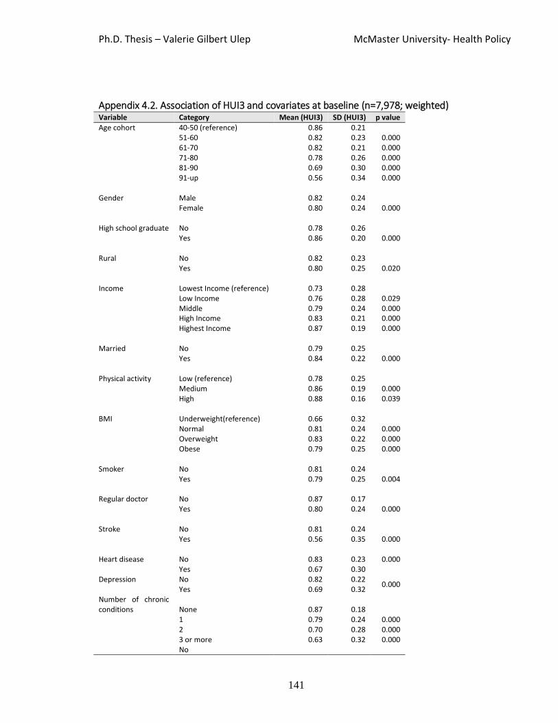
Ph.D. Thesis – Valerie Gilbert Ulep McMaster University- Health Policy
141
Appendix 4.2. Association of HUI3 and covariates at baseline (n=7,978; weighted) Variable Category Mean (HUI3) SD (HUI3) p value Age cohort 40-50 (reference) 0.86 0.21 51-60 0.82 0.23 0.000 61-70 0.82 0.21 0.000 71-80 0.78 0.26 0.000 81-90 0.69 0.30 0.000 91-up 0.56 0.34 0.000 Gender Male
0.82
0.24
0.000 Female 0.80 0.24 High school graduate No
0.78
0.26
0.000 Yes 0.86 0.20 Rural No
0.82
0.23
0.020 Yes 0.80 0.25 Income Lowest Income (reference)
0.73
0.28
Low Income 0.76 0.28 0.029 Middle 0.79 0.24 0.000 High Income 0.83 0.21 0.000 Highest Income 0.87 0.19 0.000 Married No
0.79
0.25
0.000 Yes 0.84 0.22 Physical activity Low (reference)
0.78
0.25
Medium 0.86 0.19 0.000 High 0.88 0.16 0.039 BMI
Underweight(reference)
0.66
0.32
Normal 0.81 0.24 0.000 Overweight 0.83 0.22 0.000 Obese 0.79 0.25 0.000 Smoker No
0.81
0.24
0.004 Yes 0.79 0.25 Regular doctor No
0.87
0.17
0.000 Yes 0.80 0.24 Stroke
No
0.81
0.24
0.000 Yes 0.56 0.35 Heart disease No
0.83
0.23 0.000
Yes 0.67 0.30 Depression No 0.82 0.22
0.000 Yes 0.69 0.32 Number of chronic conditions None
0.87
0.18
1 0.79 0.24 0.000 2 0.70 0.28 0.000 3 or more 0.63 0.32 0.000 No

Ph.D. Thesis – Valerie Gilbert Ulep McMaster University- Health Policy
142
Diabetes 0.82 0.23 0.000 Yes 0.66 0.33
Diabetes (Cycle 3) No (reference)
0.74
0.34
Lifestyle 0.71 0.34 0.003 Oral medication 0.66 0.35 0.000 Insulin 0.55 0.38 0.000 no reported 0.38 0.44
Note: We use Bonferroni’s pairwise comparison to test whether there is significant difference
between reference and a particular category

Ph.D. Thesis – Valerie Gilbert Ulep McMaster University- Health Policy
143
Appendix 4.3.a. Fixed effects coefficients and fit indices of growth models of HUI3 Trajectories, by sex (n=7,978; weighted)
Variables Female Male
Model 1 Model 2 Model 1 Model 2
Fixed effects
Age (centered) 1 0.00 0.00 0.00 0.00 0.00 0.00 0.00 (0.00) Age X Age (centered) -1.78X10-4* 0.00 -3.67X10⁻⁴*** -1.11X10-4* 0.00 0.00 0.00 0.00 Age X Age X Age (centered) -2.82X10⁻⁵*** -7.25X10⁻⁶*** -2.66X10⁻⁵*** -5.89X10-6* 0.00 0.00 0.00 0.00 Cohort 2 (Ref: Cohort 1) 2 0.00 0.02 -0.02 -0.01 (0.02) (0.01) (0.02) (0.01) Cohort 3 0.00 0.03 0.02 -0.02 (0.03) (0.02) (0.03) (0.02) Cohort 4 0.16 0.02 0.35** -0.04 (0.08) (0.06) (0.11) (0.07) Cohort 5 0.26 -0.32* 0.37 -0.48** (0.22) (0.14) (0.45) (0.17) Cohort 6 0.43 -1.88*** -1.29 -1.17* (0.70) (0.52) (0.94) (0.49) (0.02) (0.02) (0.03) (0.02) Diabetes -0.06** -0.04** -0.02 -0.01 (0.02) (0.02) (0.02) (0.01) Diabetes X Age (centered) 0.00 0.00 0.00 0.00 (0.00) (0.00) (0.00) (0.00) White 0.25*** 0.07*** 0.27*** 0.05*** (0.03) (0.01) (0.03) (0.01) High school graduate 0.07*** 0.05*** 0.07*** 0.02** (0.01) (0.01) (0.01) 0.01 Rural 0.04*** -0.01 0.06*** -0.01 (0.01) (0.01) (0.01) (0.01) Married 0.01 0.00 0.031* 0.02* (0.01) (0.01) (0.01) (0.01) Low Income (Ref: Lowest Income) -0.01 0.00 0.07*** 0.03* (0.01) (0.01) (0.02) (0.01) Middle Income 0.02 0.02 0.05* 0.01 (0.02) (0.01) (0.02) (0.02) High Income 0.00 0.02* 0.08*** 0.03* (0.02) (-0.01) (-0.02) (-0.01) Highest Income 0.01 0.03** 0.09*** 0.05*** (0.02) (0.01) (0.02) (0.01) Physical activity – Medium (Ref: Low) 0.05*** 0.04*** 0.03*** 0.01** (0.01) (0.01) (0.01) (0.01) Physical activity - High 0.04*** 0.04*** 0.05*** 0.03*** (0.01) (0.01) (0.01) (0.01) Smoker -0.02 -0.03*** -0.01 -0.01 (0.01) (0.01) (0.02) (0.01) BMI – overweight (Ref: Underweight and normal) 0.03** 0.02** 0.05*** 0.01* (-0.01) (-0.01) (-0.01) (-0.01) BMI - Obese 0.02 0.00 0.04* 0.00 (0.01) (0.01) (0.02) (0.01) Regular doctor -0.02 -0.01 -0.01 -0.01 (0.01) (0.01) (0.02) (0.01) Heart disease -0.07*** -0.04*** -0.04* -0.03***

Ph.D. Thesis – Valerie Gilbert Ulep McMaster University- Health Policy
144
(0.02) (0.01) (0.02) (0.01) Stroke -0.15*** -0.10*** -0.16*** -0.09*** (0.03) (0.02) (0.03) (0.02) Depression -0.05*** -0.05*** -0.08*** -0.08*** (0.01) (0.01) (0.02) (0.01) 1 chronic condition (Ref: None) 3 -0.04*** -0.04*** -0.04*** -0.03*** (0.01) (0.01) (0.01) (0.01) 2 chronic condition -0.08*** -0.06*** -0.08*** -0.06*** (0.01) (0.01) (0.01) (0.01) 3 or more chronic condition -0.16*** -0.12*** -0.13*** -0.12*** (0.02) (0.01) (0.02) (0.01) Institutionalized -0.04 -0.42*** -0.02 -0.42*** (0.03) (0.03) (0.04) (0.04) Dead -0.65***
-0.70***
(0.01) (0.01) Random Effects
Inter-individual variance Age (slope) 7.02X10⁻⁵ 4.11X10⁻⁷ 1.82X10⁻⁵ 1.51X10⁻¹³ Age X Age (slope) 1.15X10⁻⁷ 4.72X10⁻¹⁵ 9.62X10⁻⁸ 9.40X10⁻²¹ Age X Age X Age (slope) 3.21X10⁻¹⁰ 1.06X10⁻¹¹ 5.76X10⁻¹⁰ 1.23X10⁻¹¹ Intercept 0.03 0.01 0.03 0.01 Intra-individual variance 0.04 0.03 0.05 0.02 AIC 4 90.24 47.83 91.61 51.55 BIC 4 442.40 408.40 434.10 402.20
Note:
Model 1 – controlled for all covariates except mortality. Model 2- controlled for all covariates including mortality. Coefficients and standard error is in parenthesis.
* p<0.05 *** p<0.001 1Median-entered. Median is 52 2We also interacted age and cohort but not shown in the table 3 Chronic conditions other than stroke, heart disease and depression 4Akaike information criterion (AIC) and Bayesian information criterion (AIC) are criteria to measure goodness of fit, and use for model selection. Lower values of AIC and BIC are desirable.

Ph.D. Thesis – Valerie Gilbert Ulep McMaster University – Health Policy
145
Appendix 4.3.b. Fixed effects coefficients and fit indices of growth models of HUI3 Trajectories using diabetes with treatment type Variables Model 1 Model 2
Age X Age (centered)1 -0.0002* -0.000 (0.00) (0.00) Age X Age X Age (centered) 3.21x10⁻⁶*** 8.51X10⁻⁶*** (0.00) (0.00) Cohort 22 -0.015 0.01 (0.02) (0.01) Cohort 3 -0.12** -0.02 (0.04) (0.02) Cohort 4 -0.04 -0.08 (0.12) (0.07) Cohort 5 -0.13 -0.53** (0.30) (0.16) Cohort 6 -1.06 -1.06** (1.43) (0.35) Diabetes -lifestyle change (Ref: No diabetes) -0.06 -0.06 (0.04) (0.04) Diabetes-oral medication 0.01 0.00 (0.02) (0.01) Diabetes -insulin therapy -0.07 -0.04* (0.04) (0.02) Diabetes - no therapy reported -0.09** -0.01 (0.03) (0.01) Diabetes -lifestyle change X age 0.00 0.00 (0.01) (0.00) Diabetes -oral medication X age -0.00** -0.00 (0.00) (0.00) Diabetes -insulin therapy X age 0.00 0.00 (0.00) (0.00) Diabetes - no therapy reported X age 0.00 0.00* (0.00) (0.00) female 0.07*** 0.02** (0.01) (0.01) white 0.36*** 0.065*** (0.03) (0.01) High school graduate 0.07*** 0.04*** (0.01) (0.01) Rural 0.02* -0.00 (0.01) (0.00) Married 0.02* 0.01 (0.01) (0.01) Low Income (Ref: Lowest Income) 0.03* 0.01 (0.01) (0.01) Middle Income 0.03 0.02* (0.02) (0.01)

Ph.D. Thesis – Valerie Gilbert Ulep McMaster University – Health Policy
146
High Income 0.02 0.02* (0.01) (0.01) Highest Income 0.04** 0.04*** (0.01) (0.01) Physical activity – Medium (Ref: Low) 0.04*** 0.03*** (0.01) (0.00) Physical activity - High 0.04*** 0.03*** (0.01) (0.01) Smoker -0.02 -0.02*** (0.01) (0.01) BMI – overweight (Ref: Underweight and normal) 0.03*** 0.01* (0.01) (0.01) BMI - Obese 0.02* -0.01 (0.01) (0.01) Regular doctor -0.01 -0.01 (0.01) (0.01) Heart disease -0.06*** -0.03*** (0.01) (0.00) Stroke -0.14*** -0.10*** (0.02) (0.01) Depression -0.06*** -0.06*** (0.01) (0.01) 1 chronic condition (Ref: None)3 -0.04*** -0.03*** (0.01) (0.00) 2 chronic condition -0.08*** -0.06*** (0.01) (0.01) 3 or more chronic condition -0.16*** -0.12*** (0.02) (0.01) Institutionalized -0.03 -0.44*** (0.02) (0.03) Dead -0.67*** (0.01) AIC4 102.30 39.13 BIC4 528.50 474.00
Note: Model 1 – controlled for all covariates except mortality. Model 2- controlled for all covariates including mortality. Coefficients and standard error is in parenthesis
* p<0.05 *** p<0.001 1Median-entered. Median is 52 2We also interacted age and cohort but not shown in the table 3 Chronic conditions other than stroke, heart disease and depression 4Akaike information criterion (AIC) and Bayesian information criterion (AIC) are criteria to measure goodness of fit, and use for model selection. Lower values of AIC and BIC are desirable.

Ph.D. Thesis – Valerie Gilbert Ulep McMaster University – Health Policy
147
Appendix 4.4. Unpacking HUI3
The table below shows the prevalence of severity of individual attributes by diabetes
status. The proportion of population with severe problem is higher among persons with
diabetes. The relatively higher prevalence of severe problem among persons with
diabetes is noted on the following attributes: cognition (33.2%), pain (36.4%) and
ambulation (23.1%).
Distribution of the severity of HUI3 attributes, by diabetes status (Cycle 1)
Severity Vision Hearing Emotion Cognition Pain Speech Ambulation Dexterity
ND D ND D ND D ND D ND D ND D ND D ND D
No problem (%) 24 17 80 79 75 71 69 63 78 57 99 98 92 77 98 97 Moderate problem (%) 72 72 5 8 22 22 3 4 4 7
Severe problem (%) 5 11 6 14 4 8 29 33 18 36 1 2 8 23 2 3
Note: ND (Without diabetes); D (With diabetes). Each attribute has 6 levels. However, we re-categorized them to three because of sample size limitation. We further merged the categories moderate and severe in Speech, Ambulation and Dexterity into two.

Ph.D. Thesis – Valerie Gilbert Ulep McMaster University – Health Policy
148
The table below shows the prevalence of impaired attributes among persons with
diabetes disaggregated by gender. Note that impaired emotion, impaired cognition and
pain might be driving the lower HUI3 scores among females.
Prevalence (%) of impaired HUI3 attributes among persons with diabetes, by cycle and
gender
Attributes Cycle 1 Cycle 2 Cycle 3 Cycle 4 Cycle 5 Cycle 6 Cycle 7 Cycle 8 Cycle 9
M F M F M F M F M F M F M F M F M F
Vision 82 82 77 91 84 85 79 84 79 86 76 89 76 89 76 87 80 85 Hearing 9 9 12 8 13 12 8 6 11 8 10 9 8 8 9 9 14 13 Mobility 12 16 16 18 15 20 17 19 17 24 15 27 12 26 19 28 15 26 Emotion 26 35 26 32 33 30 34 32 32 29 34 33 25 29 32 33 29 28 Cognition 35 41 31 35 35 43 36 34 34 34 34 36 38 34 34 41 35 35 Pain 37 51 28 39 30 36 29 30 32 40 26 37 22 31 32 33 30 28
Note: M (Male); F(Female). We excluded speech and dexterity due to sample size limitation.

Ph.D. Thesis – Valerie Gilbert Ulep McMaster University – Health Policy
149
The table below shows that female with diabetes, on average, experience more number
of co-morbidities than males with diabetes. Further, the prevalence of chronic
conditions that are highly related to mortality is higher among female with diabetes
than male with diabetes.
Average number and prevalence of chronic condition among person with diabetes, by gender
Cycle 1 Cycle 2 Cycle 3 Cycle 4 Cycle 5 Cycle 6 Cycle 7 Cycle 8 Cycle 9
Average number of chronic condition among persons with diabetes
Male 1.3 1.8 1.7 1.8 1.8 1.8 2.1 2.0 2.2
Female 2.2 2.4 2.5 2.6 2.8 2.8 3.0 3.0 3.1
Chronic conditions related to mortality (%)
Male 37 45 42 47 49 51 60 55 57
Female 54 53 58 61 62 65 68 67 69
Chronic conditions that may be related to mortality (%)
Male 1 11 5 8 9 10 10 11 13
Female 8 15 16 17 18 20 21 22 22
Conditions not related to mortality (%)
Male 45 57 48 52 53 55 56 54 58
Female 59 66 72 68 70 72 72 72 73
Note: Conditions related to mortality include high blood pressure, chronic bronchitis or emphysema. Conditions that may be related to mortality include Asthma, Alzheimer’s disease or dementia. Conditions that not related to mortality include food allergies, allergies other than food allergies, arthritis or rheumatism, back problems excluding arthritis, migraine headaches, sinusitis, epilepsy, stomach or intestinal ulcers, urinary incontinence, cataracts, glaucoma, and other long-term condition.

Ph.D. Thesis – Valerie Gilbert Ulep McMaster University – Health Policy
150
Chapter 5: Conclusion
In Chapter 2, we examined the impact of the national health insurance program
of the Philippines on maternal and health outcomes among poor Filipino mothers. In
Chapter 3, we evaluated the impact of Jamkesmas, the largest subsidized health
insurance Indonesia on wide-range of healthcare utilization, health outcomes, and
healthcare expenditures. In Chapter 4, we characterized the age-related-trajectories of
health-related quality of life of Canadians with diabetes.
In Chapter 2, we found that national health insurance program in the Philippines
is associated with more prenatal care visits, greater likelihood of facility-based birth
delivery, and more post-natal care, and the impact is most pronounced among the
poorest women. However, we did not observe improvements in birthweight.
In Chapter 3, we found that Jamkesmas is associated with higher likelihood of
outpatient care, but we did not observe heterogeneity across income groups. Among
those who had outpatient care, Jamkesmas is also associated with higher number of
outpatient care visits. Jamkesmas is also associated with higher likelihood of inpatient
care, with larger impact among the rich. However, we did not observe a statistically
significant impact on health outcomes even adjusting for temporal effects. We observed
lower out-of-pocket healthcare expenditure but no impact on catastrophic healthcare
expenditures.

Ph.D. Thesis – Valerie Gilbert Ulep McMaster University – Health Policy
151
Our findings in Chapters 2 and 3 provide an important insight that despite
improvements in healthcare utilization and reduction in out-of-pocket healthcare
expenditures, health insurance may not improve health outcomes. In Chapter 3, we also
found heterogeneity in impact on inpatient care. We observed large and statistically
significant impact among the rich, but no statistically significant impact among the poor.
This is a potential indication that the poor might not have benefitted from the expansion
of Jamkesmas. We observe mistargeting in the program, meaning a number of the rich
population were covered, a problem also common in the Philippine national health
insurance.
In Chapter 4, we found that the poor and women with diabetes experience a
lower health-related quality of life trajectories, but there is no evidence that the rate of
deterioration of their health-related quality of life is faster than for individuals without
diabetes. Our finding differs from a trajectory study conducted in the United States,
where significantly faster deterioration was observed among individuals with diabetes
(Chiu & Wray, 2010). The study provides evidence that individuals with diabetes have
the ability the ‘compress morbidity’ and sustain a rate of deterioration similar to healthy
individuals.