Essays on Public and Environmental Economics

Item Type text; Electronic Dissertation

Authors Burr, Chrystie T.

Publisher The University of Arizona.

Rights Copyright © is held by the author. Digital access to this materialis made possible by the University Libraries, University of Arizona.Further transmission, reproduction or presentation (such aspublic display or performance) of protected items is prohibitedexcept with permission of the author.

Download date 11/07/2018 04:29:55

Link to Item http://hdl.handle.net/10150/293611

ESSAYS ON PUBLIC AND ENVIRONMENTAL ECONOMICS

by

Chrystie T. Burr

BY:© =©

A Dissertation Submitted to the Faculty of the

DEPARTMENT OF ECONOMICS

In Partial Fulfillment of the RequirementsFor the Degree of

DOCTOR OF PHILOSOPHY

In the Graduate College

THE UNIVERSITY OF ARIZONA

2013

2

THE UNIVERSITY OF ARIZONAGRADUATE COLLEGE

As members of the Dissertation Committee, we certify that we have read the dis-sertation prepared by Chrystie T. Burrentitled Essays on Public and Environmental Economicsand recommend that it be accepted as fulfilling the dissertation requirement for theDegree of Doctor of Philosophy.

Date: 29 April 2012Rabah Amir

Date: 29 April 2012Price Fishback

Date: 29 April 2012Gautam Gowrisankaran

Date: 29 April 2012Derek Lemoine

Date: 29 April 2012Paul Portney

Final approval and acceptance of this dissertation is contingent upon the candidate’ssubmission of the final copies of the dissertation to the Graduate College.I hereby certify that I have read this dissertation prepared under my direction andrecommend that it be accepted as fulfilling the dissertation requirement.

Date: 29 April 2012Dissertation Director: Gautam Gowrisankaran

3

STATEMENT BY AUTHOR

This dissertation has been submitted in partial fulfillment of requirements for anadvanced degree at the University of Arizona and is deposited in the UniversityLibrary to be made available to borrowers under rules of the Library.

Brief quotations from this dissertation are allowable without special permission,provided that accurate acknowledgment of source is made. This work is licensedunder the Creative Commons Attribution-No Derivative Works 3.0 United States Li-cense. To view a copy of this license, visit http://creativecommons.org/licenses/by-nd/3.0/us/ or send a letter to Creative Commons, 171 Second Street, Suite 300,San Francisco, California, 94105, USA.

SIGNED: Chrystie T. Burr

4

ACKNOWLEDGEMENTS

This dissertation would not have been possible without the guidance by GautamGowrisankaran and Rabah Amir. I also thank the support and comments fromFerenc Szidarovszky, Paul Portney, Derek Lemoine and Price Fishback.

5

DEDICATION

To my beloved family

6

TABLE OF CONTENTS

Page

LIST OF FIGURES . . . . . . . . . . . . . . . . . . . . . . . . . . . . . . . . 8

LIST OF TABLES . . . . . . . . . . . . . . . . . . . . . . . . . . . . . . . . . 9

ABSTRACT . . . . . . . . . . . . . . . . . . . . . . . . . . . . . . . . . . . . 10

CHAPTER 1 SUBSIDIES, TARIFFS AND INVESTMENTS IN THE SOLARPOWER MARKET . . . . . . . . . . . . . . . . . . . . . . . . . . . . . . 121.1 Introduction . . . . . . . . . . . . . . . . . . . . . . . . . . . . . . . . 121.2 Background Information . . . . . . . . . . . . . . . . . . . . . . . . . 16

1.2.1 The Characteristics of Solar Technology . . . . . . . . . . . . 161.2.2 Solar Power Markets . . . . . . . . . . . . . . . . . . . . . . . 181.2.3 Incentive Designs . . . . . . . . . . . . . . . . . . . . . . . . . 191.2.4 California Solar Initiative Program . . . . . . . . . . . . . . . 21

1.3 Data . . . . . . . . . . . . . . . . . . . . . . . . . . . . . . . . . . . . 231.4 The Structural Model . . . . . . . . . . . . . . . . . . . . . . . . . . . 281.5 Estimation . . . . . . . . . . . . . . . . . . . . . . . . . . . . . . . . . 321.6 Counterfactual Analysis . . . . . . . . . . . . . . . . . . . . . . . . . 37

1.6.1 Welfare Analysis of the Current Incentive Programs . . . . . . 371.6.2 Deadweightloss resulting from suboptimal siting . . . . . . . . 401.6.3 Impacts from Policy Changes . . . . . . . . . . . . . . . . . . 41

1.7 Conclusion . . . . . . . . . . . . . . . . . . . . . . . . . . . . . . . . . 42

CHAPTER 2 CORRUPTION AND SOCIALLY OPTIMAL ENTRY . . . . 442.1 Introduction . . . . . . . . . . . . . . . . . . . . . . . . . . . . . . . . 442.2 The model and the benchmarks . . . . . . . . . . . . . . . . . . . . . 49

2.2.1 Free entry . . . . . . . . . . . . . . . . . . . . . . . . . . . . . 512.2.2 Second best socially optimal entry . . . . . . . . . . . . . . . . 512.2.3 Corruption induced monopoly . . . . . . . . . . . . . . . . . . 52

2.3 Single official in a pre-existing market . . . . . . . . . . . . . . . . . . 552.4 Competition amongst officials . . . . . . . . . . . . . . . . . . . . . . 60

2.4.1 The case of a new industry . . . . . . . . . . . . . . . . . . . . 612.4.2 The case of a pre-existing industry . . . . . . . . . . . . . . . 65

2.5 Conclusion . . . . . . . . . . . . . . . . . . . . . . . . . . . . . . . . . 67

TABLE OF CONTENTS – Continued

7

APPENDIX A APPENDIX TO CHAPTER 1 . . . . . . . . . . . . . . . . . 70A.1 Hedonic Regression Results . . . . . . . . . . . . . . . . . . . . . . . 70

A.1.1 Factors that Influence Investment Decisions . . . . . . . . . . 70A.2 Full Tables . . . . . . . . . . . . . . . . . . . . . . . . . . . . . . . . . 74A.3 Calculating the equivalent CO2 prices from deadweightloss . . . . . . 81A.4 Parameter Calibration and Data Cleaning . . . . . . . . . . . . . . . 82A.5 On Deriving the Logit Inclusive Value . . . . . . . . . . . . . . . . . . 83A.6 Figures and Charts . . . . . . . . . . . . . . . . . . . . . . . . . . . . 84

APPENDIX B APPENDIX TO CHAPTER 2 . . . . . . . . . . . . . . . . . 93B.1 Proof of Lemma 1 . . . . . . . . . . . . . . . . . . . . . . . . . . . . . 93B.2 Proof of Proposition 1 . . . . . . . . . . . . . . . . . . . . . . . . . . 94B.3 Proof of Lemma 2 . . . . . . . . . . . . . . . . . . . . . . . . . . . . . 95B.4 Proof of Proposition 3 . . . . . . . . . . . . . . . . . . . . . . . . . . 96

REFERENCES . . . . . . . . . . . . . . . . . . . . . . . . . . . . . . . . . . . 98

8

LIST OF FIGURES

Figure 1.1 System price trend and number of installations . . . . . . . . 24Figure 1.2 Monthly installations in PG&E service territory . . . . . . . 26

Figure A.1 Grid-tied cumulative PV installed capacity in California,1996-2006 . . . . . . . . . . . . . . . . . . . . . . . . . . . . . . . . . 84

Figure A.2 Average module cost, 1975-2012 . . . . . . . . . . . . . . . 84Figure A.3 Average install system cost in the US, 1998-2012 . . . . . . 84Figure A.4 CSI 10 step subsidy schedule . . . . . . . . . . . . . . . . . 84Figure A.5 Subsidy degression in cumulative installed capacity . . . . . 84Figure A.6 Zip code map showing PV system adoptions in California . 84Figure A.7 Map showing the counties included in this study . . . . . . 84Figure A.8 Raw CSI installation data . . . . . . . . . . . . . . . . . . . 84Figure A.9 2010 benchmark residential PV system price components . 84Figure A.10 PV system size distribution . . . . . . . . . . . . . . . . . . 84Figure A.11 CSI subsidy by the three investor-owned utility territories . 84Figure A.12 Scatter plot of cost per watt versus system size . . . . . . . 84Figure A.13 System net cost and the number of installations in La Jolla,

San Diego . . . . . . . . . . . . . . . . . . . . . . . . . . . . . . . . . 84

9

LIST OF TABLES

Table 1. Summary statistics . . . . . . . . . . . . . . . . . . . . . . . . 26Table 2. Regression analysis on the installed cost per watt . . . . . . . . 34Table 3. Estimation results from the maximim likelihood estimation . . 36

Table A.1 Hedonic regression results . . . . . . . . . . . . . . . . . . . 73Table A2.1 Summary statistics (full table) . . . . . . . . . . . . . . . . 74Table A2.2 t test result of the average size from leased and non-leased

units . . . . . . . . . . . . . . . . . . . . . . . . . . . . . . . . . . . . 74Table A2.3 First stage regression result on cost per watt . . . . . . . . . 74Table A2.4 Estimation results from the maximum likelihood estimations

(full) . . . . . . . . . . . . . . . . . . . . . . . . . . . . . . . . . . . . 76Table A2.5 Welfare analysis of current subsidy programs . . . . . . . . 77Table A2.6 Counterfactual analysis with solar irradiation in Fankfur,

Germany . . . . . . . . . . . . . . . . . . . . . . . . . . . . . . . . . . 78Table A2.7 Welfare comparison between capacity-based and production-

based subsidies . . . . . . . . . . . . . . . . . . . . . . . . . . . . . . 79Table A2.8 Potential impact of the pending tariff on imported Chinese

solar cells . . . . . . . . . . . . . . . . . . . . . . . . . . . . . . . . . 79Table A2.9 Potential impacts from varying incentive levels . . . . . . . 79Table A4.1 Overall component DC-AC derate factor . . . . . . . . . . . 82Table A4.2 Assumption in simulating the future revenue and costs . . . 82

10

ABSTRACT

Over the last 10 years, the solar photovoltaic (PV) market has experienced tremen-

dous growth due in part to government incentive programs. However the effect and

welfare analysis of these policy instruments remain ambiguous. In the first chapter

of my dissertation, we estimate a dynamic model of household’s investment decisions

on rooftop PV systems to understand the impact of these programs on residential

solar installations and evaluate the outcome of alternative incentive policies. The

model separately evaluates the effect of system prices, up-front subsidies, tax credits

and production revenues using a 5-year data set collected by the California Solar

Initiative program, which subsidized solar installations in California. The results

indicate that capacity-based subsidies are equally effective as production-based sub-

sidies, but that the latter are more efficient. With a $100 social cost of carbon,

the total subsidies in California would be welfare neutral. If California were only

as sunny as Frankfurt, Germany, this value has to be $200 to be welfare neutral.

We find that without subsidies, 85% of the existing installations would not have

occurred. The second chapter of my dissertation is on the political economics of

corruption. This is a relevant question in the Environmental Economics due to

the human factors involved in government regulations. We investigate the effects

of unhindered corruption in the entry-certifying process of an industry on market

structure and social welfare. To gain entry, a firm must pay a bribe-maximizing

official an exogenous percentage of anticipated profit, in addition to the usual set

up cost. This would lead to a monopoly, but only in markets without pre-existing

firms. A benevolent social planner may use bribery to the benefit of society by

either manipulating the number of pre-existing firms in the market, or by setting

up independent (corrupt) licensing authorities. A socially optimal number of firms

in the market may be reached by choosing the right number of pre-existing firms

11

or by having exactly two licensing authorities. These mechanisms may be seen as

restoring second-best efficiency in settings characterized by two major sources of

distortion: Imperfect competition and corruption.

12

CHAPTER 1

SUBSIDIES, TARIFFS AND INVESTMENTS IN THE SOLAR POWER

MARKET

1.1 Introduction

”I’d put my money on the sun and solar energy. What a source of power! I

hope we don’t have to wait until oil and coal run out before we tackle that.”

-Thomas Edison, 1931

”Photovoltaics are threatening to become the costliest mistake in the history

of German energy policy.” -Der Spiegel, July 4, 2012

Over the past decade, solar photovoltaic (PV) became the fastest growing renewable

energy technology available, with an annual growth rate of 50%.1 There are two

primary drivers behind this growth: 1) a sharp reduction in the costs of solar PV

systems, and 2) government incentive programs to promote PV installations. Lev-

elized costs2 have dropped an order of magnitude in the last 30 years, from $2/kWh

in 1980 to $0.21/kWh in 2011. Even with this substantial decrease in costs, most

solar installations would still not be competitive however, since the levelized costs

of coal and natural gas remain lower, at about 6 cent/kWh (Borenstein, 2011). The

solar PV market has overcome this cost difference through government incentive

programs. In 2010, The U.S. federal government spent $14.67 billion on subsidizing

renewable energy (EIA, 2011).3 California set aside $3.35 billion dollars to subsidize

1The growth here refers to additional operating capacity installed. Internationally the growthrate of solar operating capacity is much higher at an average rate of 80%

2Levelized cost of energy or LCOE is the present value of the per unit electricity cost for thelifespan of the electricity generator. It reflects both fixed and variable costs.

3This subsidy amount includes direct expenditures to producers or consumers, tax expenditures,R&D, loans and loan guarantees. In particular, one billion dollars are spent on solar subsidies while6 billion dollars go towards subsidizing biofuels.

13

rooftop solar power system adoptions. Meanwhile Germany, the worlds leader in

solar adoptions, expects to invest over $11 billion on production subsidies in 2012.4

While various government entities in the U.S. and worldwide have spent huge

amounts subsidizing solar energy technologies, the effectiveness and the welfare

costs associated with the subsidy programs remain ambiguous. Many incentive pro-

grams, such as in California, provide upfront capacity-based subsidies that depend

on the size of the installed systems. Other programs, such as in Germany, pro-

vide production-based subsidies that depend on the amount of electricity generated.

The success in stimulating solar adoptions in Germany has lead to many inconclu-

sive discussions on whether production-based subsidies are the cost-effective policy

instruments to accelerate the diffusion of renewable energy technologies.5 More gen-

erally, little is known about the amount of CO2 that is offset by each subsidy dollar

under different programs.

In this paper, we develop a dynamic consumer demand model for rooftop solar

power systems. Each household solves an optimal stopping problem when making

the investment decision in solar power systems. The model assumes that house-

holds can perfectly forecast future system prices and subsidies while evaluating the

benefit of investing today versus the benefit of waiting. We use a nested fixed-point

maximum likelihood estimation on a 5-year data set from California to recover the

underlying structural parameters in the consumer demand function. The model

separately evaluates the impact of capacity-based subsidies, tax credits and the rev-

enues raised by electricity production. Since production-based subsidies provide a

premium over the retail electricity rate, the effect of the revenue generated from so-

lar electricity is assumed to be identical to the effect of revenue generated with the

additional premium. The variations in solar irradiation across California and the

4Germany has on average half of the solar resources, one quarter of the population and onefifth of the GDP compared to the U.S. However its solar deployment (in cumulative installed PVcapacity)is 6 times higher than it is in the U.S.

5Sir Nicholas Stern commented in his famous and controversial Stern Review that ”feed-in mech-anisms achieve larger deployment at lower costs”, when considering the long-term price guaranteeassurance affect, and by comparison with tradable renewable energy certificates (RECs). Manysubsequent policy discussions extend such favoritism to FIT, over all alternative instruments.

14

changes in PV module prices, capacity-based subsidies, tax credits and electricity

rates through time enable me to identify the impact of each variable.

We use this estimated model to address questions concerning the economic value

of solar PV incentive programs. The first goal of this paper is to investigate whether

there is any empirical evidence to support the claim that production-based subsidies

are cost-effective instruments to stimulate demand in the solar market. The second

goal is to study how each policy instrument affects social welfare and whether one

policy is more efficient than another. Efficiency in this context is measured by the

amount of CO2 displaced as the consequence of the incentive policy. The results

indicate that a capacity-based subsidy is at least as effective as a production-based

subsidy if not better. In terms of welfare however, production-based subsidies are

more efficient as they encourage more adoptions in optimal locations for solar elec-

tricity production.

Next, we examine demand-side responses to subsidy policy changes. These

changes include varying the subsidy level so that the implied CO2 price matches

the social cost of carbon6. The equivalent CO2 price of the aggregate subsidy in

California is currently at $100/ton. If the subsidies were to decrease to the equiva-

lent level of $21/ton social cost of carbon as suggested by Greenstone et al. (2011),

we can expect a drastic reduction of 85% in installations. A significant pending pol-

icy change for the solar PV market in the U.S. is an antidumping tariff on imported

Chinese solar cells. In October 2011, a coalition led by SolarWorld, a German-

headquartered solar manufacturer, filed an unfair competition complaint with the

U.S. Department of Commerce (DOC) and International Trade Commission (ITC),

which led to a ruling that will impose an up to 250% duty on solar cells manufac-

tured in China. It is a ruling that splits the U.S. solar industry between domestic

6The derivation of social cost of carbon (SSC) measures the economic damage that is associatedwith each ton7 of CO2 released into the atmosphere. It requires significant assumptions that covera wide range of fields, including: Atmospheric Science, Agriculture, Geosciences, Economics, etc.One of most important assumptions is on the discount rate used in order to calculate the presentvalue of future damages. Greenstone et al. (2011) used a 3% discount rate and found the SSC tobe the $21/ton (in 2007 dollar) while the Stern Review used a lower discount rate of 1.4% to findthe SSC price to be $111/ton (in 2011 dollars).

15

manufacturers and solar power system installers who depend on Chinese solar prod-

ucts. The latter group is concerned that the increase in solar system costs will have

a detrimental effect on the growth of the solar power market. This paper assesses

the potential impact of a higher system price induced by the pending tariff.

The quotes above encompass the conundrum in solar PV subsidies faced by

policy makers. On the one hand, there is a consensus to expedite the transition from

finite energy resources to renewable resources, with their reduced levels of criteria

pollutants and greenhouse gases. On the other hand, it is difficult to design and

implement a sustainable policy that balances growth with spending. The advantages

of any subsidy policy must be weighed by its costs, or it will be doomed to failure.

To assess the costs associated with solar adoptions in suboptimal locations, we

conducted a counterfactual analysis on the California market assuming the same

solar irradiation as in Frankfurt, Germany. We found that with the current subsidy

program, the implied CO2 price would effectively double. In addition, if the number

of installations and electricity production were to reach the current levels seen in

California, equivalent CO2 prices would increase to $450 and $600 respectively.

This paper contributes to the small number of studies on the solar power market.

Barbose et al. (2011) provides a detailed summary of PV system cost trends across

the U.S. since 2008. Dastrup et al. (2012) examines solar home resale values and

calculate a green home premium. Bollinger and Gillingham (2012) identifies peer

effects in consumers’ solar adoption decisions. In my analysis these aspects of home

resale are not addressed explicitly, but the revenue generated from a solar power

system should capture most of the solar home premium. We do not consider peer

effects in this model since the average market share8 of solar adopters within a zip

code is less than 0.1%. The peer effect therefore would be unlikely to be significant

in my model. Another related strand of literature studies the optimal instrument

choice in environmental regulations. It covers wide-ranging topics from normative

studies (Goulder and Parry, 2008) to positive studies (Keohane et al., 1998) that

8The market here is define by the number of owner occupied household in a zip code. Arguablythe actual market is smaller due to the building, shading, liquidity constraint and the solar powersystem market share is much higher=.

16

compare market-based instruments and command-and-control instruments. Fischer

and Newell (2008) ranks a comprehensive list of policy instruments based on emis-

sion reductions, induced technology innovation, government revenues and renewable

energy production. Goulder et al. (1998) consider program costs of alternative poli-

cies in a second-best setting. This paper examines a subset of the incentive-based

instruments that encompasses subsidies for pollution abatement and is among the

first papers to study the cost-effectiveness and efficiency of policy instruments using

empirical data.

The following section provides background information on solar power technol-

ogy, the solar PV market, and the California Solar Initiative program. Section 3

describes the data used in the estimation. Section 4 presents the structural model

and section 5 shows the result. We discuss the counterfactual analysis in section

6 and section 7 concludes. Appendix 3.1.1 includes the reduced form regression

analysis of the same data set for the interested readers.

1.2 Background Information

1.2.1 The Characteristics of Solar Technology

Solar power systems can be broadly separated into two categories - PV technologies

and concentrated solar power technologies. PV technologies commonly referred to as

”solar panel” systems feature an unusual attribute among all electricity generation

technologies inasmuch as they provide distributed power generation. Photovoltaic

technologies convert sunlight directly into electricity using semiconductors that ex-

hibit the photoelectric effect. This effect was first observed by Becquerel in the 19th

century and in 1921 a Nobel Prize was awarded to Albert Einstein for his mathe-

matical description of the effect. When Chapin, Fuller and Pearson patented their

PV cell in 1954, while working at Bell Laboratories, they adopted silicon as the

semiconducting material of choice. It achieved 6% efficiency at a cost of $1,720/W.

Since then, crystalline silicon (c-Si) cells have been the most widely deployed PV

technology reaching an average efficiency of 14.4% (Hand et al. 2012).

17

The dominant PV cell manufacturers in the U.S. include the Phoenix-based First

Solar Company that uses different semiconducting materials, such as cadmium tel-

luride (CdTe) or copper indium gallium selenide (CGIS) to produce solar cells.

These products are often called thin-film PV cells because of their physical char-

acteristics as they are thinner than traditional c-Si cells. Thin films are generally

cheaper to produce and easier to integrate into a housing structure. However, due

to their relatively low efficiency rate9 they currently do not have a cost advantage

over c-Si solar cells. PV panels or PV modules are connected assemblies of multiple

PV cells which make up components of a larger PV system. These PV systems can

be installed on any residential rooftop to generate electricity to supply household

electricity needs. They are referred to as distributed generation systems since the

electricity is generated at each node without the need of transporting electricity

from a central power generation plant to individual users through power transmis-

sion lines. PV technologies always have an economic advantage in rural areas with

no transmission lines (off-grid systems).

The main disadvantage of PV technologies is that they only generate electricity

when the sun is shining.10 PV systems cannot support modern household electric-

ity needs without an electrical storage system, which can be extremely expensive.

Therefore the systems of interest in this paper are ”grid-connected” systems. These

systems generate electricity to supply a household but when the demand is higher

than the solar system can deliver, the residual demand is supplied by the usual

sources through grid/transmission lines.

Concentrated solar power (CSP) technologies use mirrors or lenses to focus sun-

light onto a receiver. The receiver contains a working fluid which transfers the

thermal energy to a heat engine that drives an electrical generator. Examples of

9Thin-film efficiency rate is around 10% for most commercially available cells depending on thematerial that is used. Prof. Yablonovitch used gallium arsenide (GaAs) as the solar cell materialand reached a record of 28.3% efficiency approaching the 33.5% Shockley-Quiesser efficiency limitof single junction solar cell. Thin-film PV cells are considered by many to be the technology ofthe future, and are sometimes referred to as ”second generation” solar cells.

10The intermittency and integration issue with solar and wind power which is not in the scopeof this study is discussed in Gowrisankaran et al. (2011), EnerNex Corp (2010), and GE Energy(2010).

18

CSP technologies include the Solar Two, a 10 MW Department of Energy demon-

stration solar tower project, and parabolic trough systems. CSP experienced very

little growth since the mid-90s and its utility-scaled deployment excludes this tech-

nology from the consideration in this paper.

1.2.2 Solar Power Markets

In order to consider the effect of a tariff on system cost, it is important to address

the different segments that are included in the PV supply side. This consists of two

interdependent markets-one is the market with PV installers as suppliers and the

other is the market with wafer, cell and module manufactures as suppliers. The for-

mer is analogous to the retailers and the latter as the wholesalers in the conventional

setting. The most important distinction between the two markets is that the former

is organized as a domestic market whereas the latter is an international market. For

example, manufacturers in China and Taiwan produced 61% of the global supply

of PV modules in 2011. This is an important observation since the price of solar

modules doesn’t depend on the domestic activity to a large extend. This avoids

the potential endogeneity concern of unobservables that encourage installations also

leads to higher system prices. The production capacity followed a period of rapid

expansion, as worldwide module manufacturing capacity increased 100-fold from

2007 to 2011 after the relief from the global bottleneck in raw silicon production.

However, the excess built-up in capacity finally lead to numerous bankruptcies and

consolidations, and this led to the DoC complaint filed by Solar World, discussed

above.

The solar PV demand market can be broadly divided into three sectors - util-

ity, commercial and residential, based on the ownership of the solar power system.

Residential systems are generally less than 10 kW due its the limited rooftop space

available whereas commercial systems are generally between 10 kW and several

MW and utility systems are often several hundred MW. The residential market

contributes to one-fifth of the operating capacities in the U.S. In this paper, we will

19

focus on residential grid-connected systems.11

1.2.3 Incentive Designs

The myriad of solar monetary incentive programs implemented in the U.S. can

be categorized into four types: 1) capacity-based subsidies, 2) production-based

subsidies, 3) renewable energy certificates, and 4) tax incentive policies.12

The capacity-based subsidy is an incentive policy that rewards every system

owner through upfront lump-sum cash rebates that are tied to the system size. For

example, a $2/W subsidy of a 5 kW system amounts to $10,000 worth of rebate

for the system owner. The production-based subsidy is an incentive program that

rewards each unit of electricity produced measured in kilowatt-hours (kWh). This

means system owners in sunnier locations, such as in San Diego, receive a larger

subsidy than a system owner living in San Francisco. Feed-in-tariff (FIT) is a

prominent example of a production-based subsidy. This program purchases solar

electricity from the system owners with a premium over the retail electricity rate.

It is the most widely adopted policy instrument in Europe, in contrast to net-

metering programs that are common in the U.S. The main difference between the two

programs is that FIT is a form of formal long-term contract with a guaranteed above

retail electricity rate while the net-metering program subsidizes solar electricity at

the retail rate.13 One important factor that leads to the rare occurrence of FIT in

11While commercial sector could be potentially more important to study for its larger marketshare, its complex nature poses much more challenges than the residential households. For example,consider a company rents a office building from the owner and pays its own electricity bills. Theowner might has incentives to install solar power systems to differentiate their office building fromthe others and charge a premium in the rent but conceivably a rare situation. Meanwhile the rentermay not have the right to install solar power systems or unwilling to invest due to the uncertaintyin the office rental duration. In addition many subsidies programs have a funding cap thus posesa problem in identification. The CSI residential program is one of the few programs that doesn’thave such a constraint.

12There are also strong support for the R&D incentive programs to address the knowledgespillover effect which is not considered in this paper.

13Hempling et al., 2010 proposed a formal definition of state-level feed-in tariffs as ”a pub-licly available, legal document, promulgated by a state utility regulatory commission or throughlegislation, which obligates an electric distribution utility to purchase electricity from an eligiblerenewable energy seller at specified prices (set sufficiently high to attract to the state the types andquantities of renewable energy desired by the state) for a specified duration; and which, conversely,

20

the US is due to the Public Utility Regulatory Policies Act of 1978 (PURPA). While

Congress creates PURPA to encourage small-scale renewable adoptions, it also sets

the maximum rate that a utility must pay a small renewable energy producer at the

utility’s avoided cost.14 This creates a challenge in setting a premium rate for the

renewables that is above the avoided cost.

One of the perceivable advantages of production-based subsidies over capacity-

based subsidies is that they provide incentives for owners to choose higher quality

solar panel systems and to maintain their systems at the optimal production level.

Production-based subsidies are also politically attractive since policy makers do not

need to spend a massive chunk of funding during one budget year. Meanwhile the

upfront capacity-based subsidy helps to alleviate the financial hurdle of the steep

upfront cost which is often around $30,000.15

Another important policy instrument to support the development of renewable

energy technologies is through the legislation of Renewable Portfolio Standards

(RPS). This policy requires the electricity producers to supply a portion of the

electricity from renewable sources. Currently there are 29 states and Washington

DC that have adopted RPS (EIA, 2012). These mandates create an incentive for

the usage and trading of the renewable energy certificate which is a proof of gen-

erating 1 megawatt (MW) of electricity from renewable energy sources. In some

states, electricity suppliers can publicly purchase the certificates in order to satisfy

the RPS requirement. This provides additional financial incentives that is similar to

a production subsidy for an independent electricity producer. RPS often indirectly

supports other forms of subsidies such as the incentives program mentioned above.

entitles the seller to sell to the utility, at those prices for that duration, without the seller needingto obtain additional regulatory permission.

14The definition of avoided cost, according to 16 USC §824a-3(d) is ”the cost to the electricutility of the electric energy which, but for the purchase from such cogenerator or small powerproducer, such utility would generate or purchase from another source.”

15There are other ways to mitigate the system financing issue such as the Property AssessedClean Energy (PACE) financing which has passed in 28 states and Washington DC since 2008.It is an alternative for the adopter to secure a loan. Under PACE, the city offers the loan topurchase the solar power system and the household pays it back through property tax bills over15 to 20-year time-span.

21

Tax-based incentives are another common instruments to encourage solar adop-

tions. These could include property or sales tax exemptions or tax credits. The U.S.

federal government offers a 30% tax credit to system owners both in the commercial

and the residential sectors which is set to expire in 2016. The unused portion of the

federal renewable energy tax credits can be carried over for 5 years.

1.2.4 California Solar Initiative Program

California, with its scenic coastline and rich natural resources, has always exercised

progressive environmental policies. For example, California passed the Solar Rights

Act back in 1979. This establishes the right of homeowners and businesses to access

sunlight in order to generate solar energy and limits the ability of local governments

or homeowner associations to prevent solar system installations. In 1998, California

is one of the first states to provide a capacity-based solar incentive policy following

the electricity deregulation. The funding for these programs is supported by the

Public Benefit Fund. It is collected by each investor-owned utility (IOU) company

based on the ratepayer’s electricity usage16 through a ”public good charge”, created

by AB1890 in 1996. There were two parallel subsidy programs that were in effect

from 1998 to December 31, 2006. California Energy Commission’s (CEC) Emerging

Renewable Program (ERP) which targets residential and small commercial solar

systems that are under 30 kW. Larger commercial systems are funded through

California Public Utilities Commission’s (CPUC) self-generation incentive program

(SGIP). There were very few adoptions in the market despite the initial $3/W

subsidy17 and the preexisting net-metering rule. Cumulative installation increased

by a mere 43% from 6 MW in 1996 level to 8.7 MW at the end of 1999.

The 2000-2001 electricity crisis presented itself as a turning point for the solar

power market in California. It heightened the awareness of the benefits of self-

16This additional charge varies by utility and customer type. It is around 0.85 cents/kWh inaddition to the electricity rate. 18% of the fund is used to support renewable energy technologieswhile 63% is used for energy efficiency related programs and the remaining 18% is for research anddevelopment projects.

17Compare this to the average $10/W total system price. Note that in 1998 there was a 50%cap on the total subsidy amount relative to the total system cost.

22

generated electricity and shifted the public opinion on renewable energy policy.

Following the crisis, California provides a 15% state tax credit for renewable energy

investments and increased the upfront subsidy to $4.50/W in 2001. Later that

year, funding for mid-sized and large projects were depleted. Within the three-year

timespan from 2000 to 2003, the cumulative grid-tied PV capacity increased by

300% (see Figure A.1 on page 85).

Since 2007, the two programs had been replaced by the Go Solar California

campaign with a goal of installing 3 GW of solar generating capacity over 10 years

with a budget of $3.35 billion. A third of the goal is designed to be fulfilled by

the New Solar Homes Partnership program that focuses on integrating solar power

systems into new housing constructions thus at a lower installation cost. The rest

of the capacity is to be met under the California Solar Initiative (CSI) program.

Systems larger than 30 kW18 are required to take the 5-year performance-based in-

centive to receive monthly payments while smaller systems are to take the expected

performance-based buydown (EPBB) subsidy and receive a one-time lumpsum up-

front payment.19 This upfront capacity-based rebate starts at $2.50/W and declines

to nil following a block schedule as shown in Figure A.4 and Figure A.5. When

the aggregate installed capacity reached a present amount, the subsidy level moves

down to the next level. The block schedule (or subsidy degression) is a method to

reflect the declining system cost in the future and additionally it encourage adop-

tions to occur sooner, rather than later. Since the panel price continues to decline

over time (See Figure A.2 and A.3), a rational forward looking consumer will always

choose to adopt at a later date, should the subsidy stay constant over time. Each

of the three IOUs receives a pre-allocated target and follows its own subsidy sched-

ule (Figure A.11). The particular block schedule adopted by CSI means that the

financial incentive declines as more capacity is installed. This particular design also

18When the CSI launched in 2007, this threshold is set at 100MW. Subsequently, this is loweredto 50 MW during 2008-2009 and 30 MW starting in 2010.

19The EPBB program is essentially a capacity-based subsidy but it weights the final subsidyamount based on the quality and installation orientation of the solar power systems. Systems lessthan 10 kW in size have to take the capacity-based subsidy while systems between 10 kW and 30kW have the option to opt into the PBI program.

23

means the policy makers have precise information on the amount of subsidy that is

required to reach the 1.94 GW target level of adoption.

1.3 Data

As shown in Figure A.6, rooftop PV system adoptions in California are concentrated

in the three largest metropolitan areas, namely: San Diego, Los Angeles and the Bay

area, in addition to Fresno and Sacramento. The geometric spread of the adoption

pattern stays about the same during the period of interest. We focus on 347 zip

codes that belong to 9 counties - one in the San Diego Gas and Electric (SDG&E)

service area, two in the Southern Califonia Edison (SCE) service area and 6 in the

Pacific Gas and Electric (PG&E) service territory (Figure A.7). Half of the zip codes

and households are located in the northern California while the remaining half in

southern California. The finest geographic resolution we observe in the data is at

the zip code level which defines the market in this study.20 The variable that display

variation at the zip code level is solar irradiation, which measures the average solar

energy received per square-meter per day. Solar irradiation ranges from the lowest

5.08 kWh/m2/day in Sebastopol, Sonoma county to the highest 6.57 kWh/m2/day

in Essex, San Bernadino, with a mean of 5.55. The data on irradiation is from

NREL PVWatts v.2 based on 40 km grid cells. In summary, the study includes over

2 million owner-occupied households and we observe 28,103 solar system adoptions

during the 63 months from January 2007 to March 2012. During this period, the

average installed system price21 decreased by 40% from $8.40/W22 to $5.67/W.

During the same period solar module price underwent a much more precipitous

decline with an average price drop of 57%. Several solar modules reached the $1/W

20See Figure A.8 which shows the selected entries from the dataset downloaded fromhttp://www.californiasolarstatistics.ca.gov/

21The upfront PV system price includes both the module and balance of system (BOS) costs.The latter cost typically includes inverter, transformer, supporting structures, mounting hardware,electrical protection devices, wiring, monitoring equipment, shipping, land, installation labor, per-mitting and fees. See Figure A.9 for a detailed breakdown

22In 2012 dollar the average installed system cost per watt is $9.37/W.

24

threshold at the end of 2011.23

Figure 1.1: System price trend and number of installations during the sampling period

PV system size varies greatly from project to project. Larger systems are cheaper

on average due to the economy of scale in the installation process. For an average

household to supply 100% of their electricity needs, a 4 to 6 kW PV system is

required. The average annual household electricity consumption is 7000 kWh/year

in California (EIA, 2012). In a sunny location such as San Diego, a 4.3 kW system

installed under optimal condition can generate roughly 7300 kWh of electricity in a

year where as it requires a 6 kW system to generate the same amount of electricity

in the Richmond neighborhood of San Francisco. In addition to the consideration of

how much electricity is to be generated from solar, there is the physical constraint of

rooftop space that is available for the solar power system. A 1 kW system requires

roughly 100 square feet of the surface area so a 5 kW system will take about half

of the roof space for a 1000 square feet house. The CSI data (Figure A.10) shows

23Every module index is slightly different. Data for this study is from Solarbuzz. BloombergNew Energy also kept a proprietary PV module index. Sologico offers monthly average moduleprice on the international spot market.

25

that the most common size observed is less than 5 kW and the average size of a

system installed during the last 5 years is 5.59 kW, which is the size that we assume

each adoption is associated with for the estimation. One of the constraints imposed

by the binary logit model proposed here is that the investments have to be made

over the homogeneous products including the size specification of the system. This

assumption can be relaxed in the future by extending the binary logit model into

multinomial logit and to allow the system size to vary over each year and zip code.

We reconstruct the upfront cost for this average size system in each county. First,

we establish the relationship between system cost per watt with the actual system

size, construction worker’s wage by county and price of solar module in the month

using regression analysis (See Table A2.3). The average system cost by county in

each month can be derived using the observed values.

Assuming a 25-year system lifespan, we recovered the revenue by finding the

present value of the amount of electricity generated, multiplied by electricity price

while taking panel degradation into account:

Rzt =1− r25

1− rQ · IRz · Ce

z · 365

where Q is the size of the solar panel in (kW) and IR is the solar irradiation

measured in kWh/m2/day. Let αD denote the degrade factor, αe be the electricity

escalation rate β as the annual discount factor and finally r = (1 − αD)(1 + αe)β.

The range of the present value of the revenue stream is between $12,000 and $18,000

under a 10% discount rate and increases to $20,462 and $31,294 under a 3% discount

rate (See Appendix on calibrated parameter values). The present value of revenue

varies with the geographical location and also through the years due to the annual

electricity rate adjustment by the utility companies. We use the average electricity

rate in this study instead of the time-of-use rate. Since solar electricity is generated

when the electricity demand is the highest, it corresponds to a higher electricity rate

which should lead to a higher estimate of the revenue than what is shown here.24

24Initially, the CSI rebate recipients are required to switch to the time-of-use (TOU) pricing.This TOU mandate is subsequently eliminated in June, 2007 after LA Times reports that themandate decreases the economic value of solar power system in SCE district. Borenstein (2007)

26

Note that we do not make an assumption on the discount rate that a household use

when they make the investment decision. Instead we calculate the present value

using various discount rates ranging from 3% to 10%.

Table 1 Summary statistics

Variable Mean Std. Dev. Min Max Obs.

System price1 44,702 4,212 34,122 51,318 21,861

Capacity-based subsidy 8,083 4,516 1,398 13,975 21,861

Present value of future revenue stream

5%: 19,578 1,649 16,729 25,585 21,861

Present value of future O&M costs2

5%: 4,809 113.4 4,533 4,986 21,861

Tax credit 8,071 4,835 2000 14,193 21,861

Elec. rate3 16.06 1.02 14.8 18.68 21,861

Irradiation4 5.55 0.28 5.08 6.57 21,861

Wage5 1,085 120 930 1253 21,861

Cost per watt 7.4 0.7 5.67 8.62 21,861

# installations 1.34 2.30 0 42 21,861

The capacity-based subsidy decreases from $2.50/W to $0.25/W in the SDG&E

and PG&E service areas, accounting for an 80% decline. This decreasing schedule

is by design in part to reflect consumer’s forward-looking behavior, which can be

observed in the data. The number of installations almost always peaks one period

before the CSI subsidy begins to decline as shown in Figure 1.2. Go Solar California

website offers easily accessible information on the remaining capacity in the current

step which facilitates consumers’ forecasting ability.

shows that the majority of PG&E adopters would be better off under the TOU rate but not sofor SCE adopters. The reason is because the SCE’s original flat rate schedule is tiered (greatermonthly electricity consumption is associated with higher electricity rate) but the TOU scheduleis not tiered.

1Total upfront PV system price after city and county tax2Including one inverter replacement cost, regular panel maintenance and increase in property

insurance cost.3cents/kWh4Solar potential/irradiation measured by kWh/m2/day5Weekly wage of construction worker by county

27

Figure 1.2: Monthly installations in PG&E service territory (dashed lines for one periodbefore the decline in subsidy)

During the sample period, the federal residential renewable energy tax credit

remains constant at the 30% level. The change came in when the American Recovery

and Reinvestment Act of 2009 removes the maximum credit cap of $2000 and allowed

households to claim the full 30% credit which was around $10,000 for a 5.59 kW

system in 2012. This is a significant change from an effective 5% of tax credit in

2008 to the 30% credit in 2009. Other than this change, there is a perfect correlation

between the tax credit and the upfront system cost by design. Despite the increase

in tax credit, the annual growth rate in newly installed capacity and in number of

installations from 2008 to 2009 doesn’t change significantly from the growth rate

during the 2007-2008 period. The total installed capacity in 2009 is a 200% increase

from 2008 while there is a 180% increase from 2007 to 2008. Number of installation

increases by 45% from 2007 to 2008 and by 43% from 2008 to 20009. However,

it does contribute to the household’s investment decision on the system size. The

majority of consumers choose a size that is less than 5 kW before 2009 and the

pattern shifts significantly in 2009. The percent difference between people buying

0-5 kW and 5-10 kW shrinks from 27% in 2008 to 16% in 2009 (see Figure A.10).

As the systems become increasingly affordable, more and more households choose to

invest in a size that is between 5-10 kW in size. In 2012, the number of households

28

that invest in the larger size bracket exceed the number of households invest in the

smaller systems. This phenomenon can perhaps be explained by the observation that

over 70% of adopters chose a solar leasing program in 2012. That is, by removing

the financing constraint, people chose to install an optimal size which is larger than

5 kW.25

1.4 The Structural Model

Next, the household’s dynamic discrete choice model is discussed. In each time

period, households observe the cost26 of the rooftop solar power system (p), the

capacity-based subsidy (s), the discounted present value of the 25-year production

revenue associated with solar electricity generation net of the O&M cost (r), and the

federal tax credit (τ). These are the state variables observed both by households and

econometricians. Denote X := {p, s, r, τ}. Given X and the other state variable,

ε, each household decides whether to install a medium-sized rooftop solar power

system or to stay with the existing utility setup. The ε is observed by households

but not by econometricians. The discrete choice in time t can be formally expressed

as,

dt =

1, install a solar power system

0, not install.

The household exits the market forever once choosing to adopt. Given the states

(X, ε), the action d and the household income Yi, the per-period utility can be

decomposed into two components based on the observability of econometricians -

ν(X, d;θ) and ε(d). ν(X, d;θ) is the utility that a household receives from installing

25A simple two sample t-test on the mean installed capacity between the third-party ownedsystems (leased units) and the non-leased units shows that system size is significantly larger underthe leased ownership (See Table A2.2). A more thorough study is necessary in order to eliminatethe selection effect on the system size selection. For example, it’s possible that the householdswho choose the solar leasing option tend to have larger house. This issue is however beyond theinterest of this paper since we assume away the decision process on the solar panel size selection.

26This refers to the total cost including the installation cost.

29

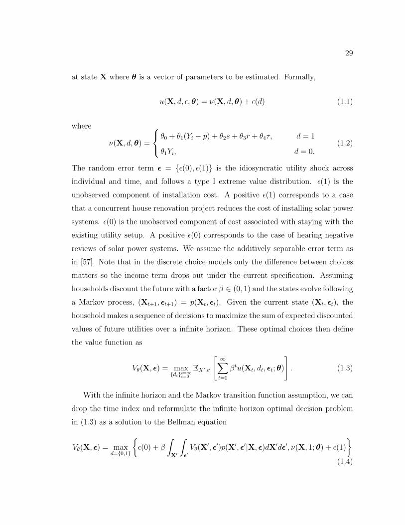
at state X where θ is a vector of parameters to be estimated. Formally,

u(X, d, ε,θ) = ν(X, d,θ) + ε(d) (1.1)

where

ν(X, d,θ) =

θ0 + θ1(Yi − p) + θ2s+ θ3r + θ4τ, d = 1

θ1Yi, d = 0.(1.2)

The random error term ε = {ε(0), ε(1)} is the idiosyncratic utility shock across

individual and time, and follows a type I extreme value distribution. ε(1) is the

unobserved component of installation cost. A positive ε(1) corresponds to a case

that a concurrent house renovation project reduces the cost of installing solar power

systems. ε(0) is the unobserved component of cost associated with staying with the

existing utility setup. A positive ε(0) corresponds to the case of hearing negative

reviews of solar power systems. We assume the additively separable error term as

in [57]. Note that in the discrete choice models only the difference between choices

matters so the income term drops out under the current specification. Assuming

households discount the future with a factor β ∈ (0, 1) and the states evolve following

a Markov process, (Xt+1, εt+1) = p(Xt, εt). Given the current state (Xt, εt), the

household makes a sequence of decisions to maximize the sum of expected discounted

values of future utilities over a infinite horizon. These optimal choices then define

the value function as

Vθ(X, ε) = max{dt}t=∞t=0

EX′,ε′[∞∑t=0

βtu(Xt, dt, εt;θ)

]. (1.3)

With the infinite horizon and the Markov transition function assumption, we can

drop the time index and reformulate the infinite horizon optimal decision problem

in (1.3) as a solution to the Bellman equation

Vθ(X, ε) = maxd={0,1}

{ε(0) + β

∫X′

∫ε′Vθ(X

′, ε′)p(X′, ε′|X, ε)dX′dε′, ν(X, 1;θ) + ε(1)

}(1.4)

30

where (X′, ε′) denotes the state variables in the next period. One of the critical

assumption proposed by [57] is the conditional independence assumption on the

transition probability p to in order to simplify the estimation complexity. This

assumption together with the additively separable error term assumption provide

the main identification strategy of the primitives.

Assumption 1. p(X′, ε′|X, ε) = pε(ε′|X′)pX(X′|X)

In another words, assumption 1 states that the unobserved state variable (by

econometricians) doesn’t affect the household’s ability to predict the future states.

Define the function, Fθ(X), as27

Fθ(X) =

∫X′

∫ε′Vθ(X

′, ε′)pε(ε′|X′)pX(X′|X)dX′dε′. (1.5)

and the choice specific value function as28

vθ(X, d) = ν(X, d, θ) + β

∫X′

∫ε′Vθ(X

′, ε′)pε(ε′|X′)pX(X′|X)dX′dε′

= ν(X, d, θ) + βFθ(X), (1.6)

or explicitly as

vθ(X, d) =

θ0 + θ1p+ θ2s+ θ3r + θ4τ, d = 1

βFθ(X), d = 0.(1.7)

The Bellman equation (1.4) can be rewritten as

Vθ(X) = maxd={0,1}

[vθ(X, d) + ε(d)] . (1.8)

Assume pε(ε′|X) is a multivariate extreme value distribution F (X) has a closed

27This function is sometimes called ”expected future utility”[65], the ”social surplusfunction”([58], McFadden 1981), or as the ”Emax function” [6] and denoted as EVθ(X, d). Inorder to avoid confusion and to emphasize that Fθ(X) is merely a function and not as a ”valuefunction”, we denote it as Fθ(X) instead.

28This term follows the common usage in the structural IO literature and with a slight abuse ofterminology since value function by definition is after choosing the optimal choice.

31

form expression which is the expected value of the maximum of 2 iid random vari-

ables.29

Fθ(X) =

∫X′

ln∑d∈0,1

evθ(X′,d)pX(X′|X)dX′ (1.9)

[58] and [59] showed (1.9) is a contraction mapping using the Blackwell’s sufficient

conditions. In addition, the conditional choice probability can now be characterized

by the binary logit formula:

Pr(d|X;θ) =exp{vθ(X, d)}

exp{vθ(X, 0)}+ exp{vθ(X, 1)}(1.10)

Pr(d = 1|Xzt ;θ) represents the probability of adopting a solar power system and

Pr(d = 0|Xzt ;θ) represents the probability of not adopting. Notice that it’s equiva-

lent to the market share definition as in [13] and therefore it’s homogeneous across

households in each zip code.

Rust(1987) proposed using the nested fixed point algorithm to estimate the struc-

tural parameter vector θ. The likelihood of observing data {Xz, di} for household i

in zip code z is

`i(Xz;θ) =

T∏t=2

Pr(dit|Xzt ;θ)p3(Xz

t |Xzt−1, d

it−1) (1.11)

The likelihood function over the whole data set is then

`θ =Z∏z=1

nz∏iz=1

`iz(Xz;θ) (1.12)

which is usually expressed as a log-likelihood function as

Lθ = log `θ =∑z

∑iz

∑t

logPr(dizt |Xzt ;θ) +

∑z

∑iz

∑t

log p3(Xzt |Xz

t−1) (1.13)

The second term is zero under the perfect foresight assumption.

29See Appendix 3.1.3 for a derivation or see Anderson et al. (1992).

32

In Rust’s nested fixed point algorithm, we optimize over (1.13) to find the deep

structural parameters θ. Formally,

maxθ

∑t

∑z

[nz(d

izt = 1) logPr(dizt = 1|Xz

t ;θ) + nz(dizt = 0) logPr(dizt = 0|Xz

t ;θ)],

(1.14)

where nz(dizt = 1) denote the total number of adoptions in a zip code, z, and

nz(dizt = 0) denote the total number of non-adopters in z. Meanwhile, in the inner

loop, the algorithm uses value function iteration to find a numerical value of Fθ(X)

computed for each value of parameters θ. Let F ζθ (X) denote numerical value during

ζth iteration. At ζ = 0, we make an initial guess of F0θ (X) = 0. At ζ = 1, we can

calculate F1θ (X) based on (1.9) and F0

θ (X), such that

F1θ (X) = T · ln

∑d∈0,1

eν(X′,d,θ)+βF0θ (X′), (1.15)

where T is the state transition matrix. Now check if the iteration has converged by

using the criterion

supX

∣∣F1θ (X)−F0

θ (X)∣∣ < ξ, (1.16)

where ξ needs to be very small such that we can minimize the amount of error

propagates from the inner-loop into the outer-loop otherwise would lead to difficulty

to converge in the outer-loop. In specific, we set ξ = 1e− 6. If the (1.16) is satisfied

then we had found the F1θ (X) to be used in (1.6) and (1.10) to go into the likelihood

function (outer-loop). If not, then repeat the iteration, let ζ = 2, 3... until the

convergence criterion (1.16) is satisfied.

1.5 Estimation

The estimation of the primitives is carried out in the following steps: In the first

stage, we recover the relationship between the dollar per watt (installed) cost of the

solar power system and its component costs. This cost per watt will be used in the

second stage in order to aggregate the data set from the individual level (however

lack of street address information) to the zip code level and in effect to conform to

33

the proposed binary logit model as discussed in the previous section. This allows us

to convert each installation observed in the data into a homogeneous medium-sized

system (5.59kW) and to derive the final installed cost associated with each system

in every zip code. The final cost can be roughly broken down into the solar module

cost (P pv), the labor cost (of installation and electricity connection) (L), the DC-

AC inverter cost(P inv), the permit fee (cfee) and electric wires and connectors cost

(BOS). We can write down the expression for cost per watt (cPw) as,

cPwizt = f(pre2007z, sizei, Ppvt , P

invt , Lcty, BOSi, c

feecty ) + εizt

Due to the economy of scale, cost per watt in general is higher for a small solar

power system and lower for a large system (see Figure A.12). It is therefore an

important factor influencing the final per watt cost. Let size denote the installed

system size observed in the data. The pre2007 variable provides the number of com-

pleted installations in a en zip code prior to the implementation of the California

Solar Initiative program in 2007. This variable is used as a proxy for many unob-

servables such as the general housing condition in a zip code or a low cost installer

located in the neighborhood. It can also potentially explain the learning by doing

effect of the installers who became more familiar with the neighborhood and the

peculiar electrical setup and thus require less time to complete the project.Sierra Club reports (2009, 2011) found that the permit fee varies from 0 to $1800

for a 3kW system with an average cost of $300.30 It’s desirable to include the permitfee in the regression however this variable is omitted due to the data constraint. Ifthe fees are constant before and after the implementation of CSI, the impact ofthis fee would be captured by the pre2007 installation term since the lower fee ina municipality/county, the more installations we would observe holding everythingelse constant. During this time period, the inverter cost remains roughly the same($.70/W according to SolarBuzz inverter retail price index) and so are the cost ofwires and connectors. In this case, the constant term captures the combined effectof these two factors. The construction workers weekly wage, published by Bureauof Labor and Statistics, acts as a proxy for the labor input cost. This wage staysabout the same in each county during the sampling period and the 5-year averagevalue is used here. Assuming linearity in all regressors except the quadratic sizeterms, the estimated result is shown in Table 2. The reconstructed system cost of a

30California state law (Government Code Section 66016) actually requires that the solar permitfee revenue can only be collected to defray the cost of processing and enforcement of the code butnot for the general revenue purpose.

34

medium-sized system is reported in Table 1. This cost is used in the second stageand also serves as the basis to derive the 30% Federal tax credits.

Table 2: Regression Analysis on Installed Cost per watt

cPw t-stat

pre2007 -0.00192∗∗∗ (-11.82)

size (kW) -0.0439∗∗∗ (-42.89)

sizeˆ2 (kW2) 0.0000508∗∗∗ (32.07)

wages 1.642∗∗∗ (36.59)

Module cost 0.936∗∗∗ (31.33)

Year FE Yes

Utility FE Yes

cons 2.016∗∗∗ (13.03)

N 73787

∗ p < 0.05, ∗∗ p < 0.01, ∗∗∗ p < 0.001

We use four specifications in the second stage structural estimation. The first

specification estimates the parameters in (1.2) and the second specification takes

into account the differences across the utility service areas. The third specification

extends the previous model to include the year fixed effects. The fourth specification

assumes that consumers don’t respond to different forms of subsidies differently. In

other words it states that a dollar from each subsidy program is treated equally as the

upfront cost. The estimation is carried out using the nested fixed point maximum

likelihood estimation of (1.13) in Matlab.31 The same results are returned under

both KNITRO and MATLAB FMINUNC optimization packages. Table A2.4 shows

the full result and Table 1 shows the results of specification 3 and 4. All estimates

have signs as expected - consumers prefer lower cost and larger subsidies except for

the tax credit term in the third specification under a 3% discount rate, which has a

insignificant negative coefficient. Under the first three specifications (I-III), upfront

31Note that the unconstrained nested fixed point MLE is identical to the constrained maximiza-tion with equality constraint (See Su and Judd (2012)). The latter has the advantage of beingfaster. Since the setup of the model is relatively simple and the contraction takes less than a halfan minute to converge, we stayed with the former approach. In the inner loop, the fixed pointalgorithm is carried out to find the expected future utility (1.5) and the outer-loop search over thewhole parameter space to find the parameter values that maximizes the log-likelihood function.

35

system cost consistently has 2 to 3 times greater adverse effect on the consumer’s

utility. Tax credit generally has the smallest impact on the household’s utility

however the relative magnitude of its effect differs across specifications.

The effect from the revenue varies under different discount rates. As expected,

the effect from the revenue becomes smaller when a low discount rate is used. This

is because with lower discount rate, the present value of the 25-year revenue stream

will be larger which leads to a smaller estimated impact coefficient. At a 10%

discount rate the revenue generates the same effect as the upfront subsidy in the

fourth specification.

The greater negative effect of the upfront system cost is as expected since it

is this particular barrier of entry that motivates creative financing strategies such

as the PACE program and solar leasing program (where consumers don’t pay the

upfront cost but pay the monthly equipment leasing fee for the next 20 years to

a commercial company). Timing that the cost incurred on the households and the

subsidies received plays a critical role on the estimated effects. Households generally

have to face the upfront cost, then the CSI rebate, follows by the tax credit and

at last the production revenue that spreads out over the next 25 years. There is

anecdotal evidence showing some installers would charge reduced upfront system

price and later collect the EPBB payment to offset this reduced charge. In that

case the timing for the upfront cost and the CSI rebate is simultaneous. However,

the most important factor that first attracts consumer’s attention is still arguably

the upfront cost. This would occur before the realization of the current CSI rebate

level. This fact remains to be verified and it can be implemented through surveying

the existing adopters.

The large variations in the estimated θ4, the tax credit effect, across models

can be contributed to the fact that the tax credit is almost perfectly correlated

with the upfront system cost. Other than the major change in 2009 when the

Federal government lifted the $2000 cap, installations would appear to be negatively

correlated with the tax credit. This is because there are more installations when the

system cost is lower and meanwhile the tax credit, as proportional to the system

cost, also appears to be lower. Figure A.13 shows that number of installations didn’t

pick up until the second quarter in 2009. Since tax credits are declared at the end of

the year, the delay in consumers’ response to the tax credit increase is reasonable.

36

Table 3: Estimation Results from Maximum Likelihood Estimation

Model Specifications with different discount rates

(III) (IV) (III) (IV) (III) (IV)

Variables 10% 10% 5% 5% 3% 3%

System cost -0.2798∗∗∗ -0.2823∗∗∗ -0.2357∗∗∗

(0.0094) (0.036) (0.0274)

Up-front subsidy 0.0996∗∗∗ 0.1023∗∗∗ 0.1244∗∗∗

(0.0104) (0.0151) (0.0131)

Revenue 0.0959∗ 0.0744 0.0707

(0.05) (0.0584) (0.0631)

Tax credit 0.1943∗∗∗ 0.1915∗ -0.0433

(0.0157) (0.0961) (0.0376)

Net cost -0.1706∗∗∗ -0.1575∗∗∗ -0.1485∗∗∗

(0.0161) (0.0178) (0.0166)

Year FE Y Y Y Y Y Y

Utility FE Y Y Y Y Y Y

constant -0.7442∗∗∗ -5.2117∗∗∗ -0.7559 -6.1794∗∗∗ -0.2214 -6.7065∗∗∗

(0.1307) (0.2495) (1.4646) (0.1708) (1.2967) (0.1356)

N observations 21861 21861 21861 21861 21861 21861

LR chi2 8410 7440 8415 7412 8364 7376

prob > chi2 0 0 0 0 0 0

standard errors in parentheses∗ p < 0.05, ∗∗ p < 0.01,∗∗∗ p < 0.001

For the first model where costs and subsidies are estimated separately, we con-

ducted three independent hypothesis testing on the null hypothesis:

(A) All four coefficients are equal (θ1 = θ2 = θ3 = θ4)

(B) three subsidy coefficients are equal (θ2 = θ3 = θ4) and,

(C) the revenue and EPBB coefficients are equal(θ2 = θ3).

With the 10% discount rate assumption, the chi-square statistic of the null hy-

pothesis C with one degree of freedom is not significant at any conventional level.

Therefore, we fail to reject the null hypothesis in this case. Null hypothesis B is

rejected at the 95% significance level and null hypothesis A is rejected at the 99.9%

significance level. This shows that if consumers use a 10% discount rate, the effect

from the capacity-based subsidy can be identical to the production-based subsidy.

37

However, capacity-based subsidy would be a cost-effective instrument if consumers

have lower discount rates. The hypothesis testing for the 5% discount rates reject

null hypothesis C at the 95% significance level and rejects the rest of the hypotheses

at the 99.9% significance level. Similar results holds for 3% discount rate as well.

The results suggest that when policy makers confront with choosing a ”cost-

effective” instrument between the capacity-based versus production-based subsidy,

the capacity-based subsidy is equally effective as production-based subsidies (at

10% discount) and more effective if consumers use a lower discount rate. Cost

effectiveness is define as the least-cost method to reach a preset target. In the case

of California Solar Initiative, this target is set at 1.94GW total installed solar power

capacities. Since this paper assumes all systems are equal in size, it is equivalent to

say that the cost-effectiveness policy here is the least-cost policy in order to reach

the target of 347,048 installations.

1.6 Counterfactual Analysis

Counterfactual analysis is carried out here to investigate 1) the welfare changes

associated with the subsidy programs and the equivalent CO2 prices and 2) the

impact of policy changes on the solar power market.

1.6.1 Welfare Analysis of the Current Incentive Programs

In order to provide a meaningful cost measure of solar incentive programs, we need

to clarify the purpose of such programs. The demand side subsidies are generally

designed to correct several types of market failures such as switching costs, liquid-

ity constraints, private discount rate being different than the public discount rate,

externalities (positive and negative), imperfect information, etc. The benefits, how-

ever, can be summarized to three common arguments that by switching to solar, we

are securing our energy independence, there will be new jobs created and the reduc-

tion in pollution emitted. The first two rationales are problematic since the main

carbon-based fuels that solar electricity substitutes for are coal and natural gas and

yet U.S. is a net exporter for both of these fuels. Although there will be new jobs

created by the green industry, there will also be jobs lost in the declining fossil fuel

sectors. Instead of creating jobs, it is perhaps more appropriate to be described as

38

shifting jobs. With regard to pollution reduction, we should focus our discussion on

the anthropogenic carbon dioxide emission since other types pollutants are mostly

under EPA regulations.32 With 40% of CO2 emission coming from the electric power

sector in the U.S., it’s reasonable to assume the main contribution of solar electric-

ity is to reduce CO2 emission and therefore to mitigate the global warming effect.

Under this measurement standard, the program cost of solar incentive programs can

be defined as the cost associated with displacing each ton of CO2 emission. The

simplest approach is to sum up the total program cost and divided the sum by the

total amount of CO2 displaced. This straightforward calculation doesn’t require

the aid of a structural model but fails to capture the change in consumer surplus

from owning a solar power system. A meaningful measure of the program cost is

then derived from finding the change in total surplus per unit pollutant avoided due

to the policy implementation. Under the assumption of a perfectly elastic supply

function, the loss in surplus is the difference between the total program spending

and the change in consumer surplus. A household makes an the investment decision

depending on which one of the two options provides the greatest utility. Yet since

there exists a part of the utility which remains unobserved to the econometrician,

the best we can do is to find the expected consumer surplus over all possible values

of ε.

E(CS) =1

θE{

maxd

[vθ(X, d) + ε(d)]}

(1.17)

where θ is the marginal utility of income and it is the marginal utility of net system

cost in the current setting. The division of θ translate utility into dollars.33 Given

the error specification of multivariate extreme value distribution, appendix A5 shows

that the expected consumer surplus has a closed form expression:

E(CS) =1

θln

[∑d=0,1

evθ(X,d)

](1.18)

Since the change in consumer surplus is derived from the dynamic model that cap-

tures the effect of a permanent change, government spending needs to be measured

32Although not addressed in this paper, the life-cycle analysis (LCA) of the technology is criticalin accessing the actual reduction in CO2 emission. NREL surveyed the past LCA studies and foundthat PV power production is similar to other renewables and much lower than fossil fuel in totallife cycle GHG emissions

33 θ = ∂U∂Y =⇒ 1

θ = ∂Y∂U

39

in the same time horizon. In order to match this long-term change in consumer sur-

plus, we aggregate the government spending over the next 100 years and discount

it with a 10%, 5% and 3% rate, respectively.34 The welfare cost associated with the

program is

PCO2 =G−4CSγ ×4Q

, (1.19)

where G is the present value of the total government spending, 4CS is change in

consumer surplus as the difference in (1.18) before and after the implementation of

the incentive policy. γ is the amount of CO2 displace by the solar power system in

its lifetime and4Q denotes the change in the number of installations due to subsidy.

Table A2.5 shows the welfare cost or the implied welfare-neutral CO2 price. With

a 3% discount rate35, the CO2 prices are $109/ton in SCE territory, $94/ton in

PG&E territory and $88/ton in SDG&E territory. The higher CO2 price in SCE

is associated with its higher upfront subsidy.36 The difference between PG&E and

SDG&E however comes solely from the difference in the ability to produce electricity.

A greater amount of electricity produced means more CO2 is abated, which serves

to lower the program cost per unit of CO2.37 This CO2 price is critical in designing

the optimal subsidy level since in the efficient outcome, the marginal abatement cost

(MAC) should equate the marginal benefit (MB). The CO2 price here is equivalent

to the MAC while the SSC is equivalent to MB.

To compare the efficiency of a production-based subsidy and a capacity-based

subsidy, we run a counterfactual analysis by investing the equivalent amount of

money into production subsidy (in present value terms) as in the current capacity-

based subsidy and observe the change in implied welfare-neutral CO2 prices. In-

tuitively a production subsidy encourages more adoptions in sunny locations and

34Discounting in itself is a subfield of environmental economics. There are many discussions onthe proper discount rate that should be used based on positive and normative arguments. See [7]for the latest summary. The broad discount rate range adopted here is in effort to provide a upperand lower bound for the impact.

35The following discussion follows the 3% discount rate scenario to be close to the discount rateused in the social cost of carbon literature

36Current CSI upfront subsidy level is still in step 7 and compared to step 9 in the other twodistricts at the end of my sample period

37In the current calculation, the average CO2 associated with each unit of electricity productionis an exogenously given constant. It’s easy to see that this value, γ, should go down as more solarpower systems are installed. However, given the solar electricity only contributes to 0.4% of totalelectricity generation. The change in γ would be insignificant for most of the years consideredhere.

40

results in a lower CO2 price. This is indeed what we observe in the analysis across all

discount rates however the difference between the capacity-based and production-

based subsidy is very small (less than $1). This is because of the relatively small

difference in solar irradiation between northern and southern California, the disutil-

ity that a consumer derives from installing solar power systems in the SCE service

area and the extremely simple (and nonoptimal) design of the FIT used in this ex-

ercise. We find that if northern California were as sunny as Newark, New Jersey

this difference will increase to a dollar. This is still not a major difference relative to

the wide range of estimated SSC prices38 calculated using different discount rates.

PVWatts data shows that there is only a 10% difference between the irradiation in

New Jersey versus the lowest radiation in the Bay area. We can expect the ineffi-

ciencies associated with capacity-based subsidy will be much greater when there is

a large variation of the solar irradiation over the country.39 The results thus show

that production-based subsidies are more efficient instrument than capacity-based

subsidies by associating with lower welfare costs.

1.6.2 Deadweightloss resulting from suboptimal siting

To address the question raised by Der Spiegel in the beginning of the paper, we

conduct a counterfactual analysis on the estimated model with the German solar

irradiation data. Suppose that the whole California is endowed with the solar ir-

radiation for Frankfurt, Germany which is 50% less than the CA solar resources.

In this case, we find the equivalent CO2 price under the current subsidy program

would be doubled to $200 (Table A2.6). In the case of having the same number

of installations as in the factual world (current point extends to the future), the

government would have to double the upfront subsidy which leads to the welfare

neutral CO2 price at $457/ton in the 3% discount rate scenario. Furthermore, in

order to have the same level of production as in the factual world, the government

has to increase the subsidy amount to three times the current level. The welfare

neutral CO2 price increases to an astonishing $600/ton under this scenario. The

38SSC estimates range from $5 to $3000. As Greenstone puts it, ”You feed a bunch of assump-tions into a machine, and out goes a number”.

39Also note that in this research, we do not incorporate the additional cost from the third-partyelectricity monitoring system that is sometimes required to report the electricity production underthe production-based subsidy. The simpler design of a capacity-based subsidy can potentiallyovercome this inefficiency.

41

result provides the first look into the high welfare cost associated with suboptimal

siting. However, the actual cost of the German subsidy program is very likely to be

smaller which ultimately depends on consumer attitudes and the amount of CO2

produced during electricity generation.40

1.6.3 Impacts from Policy Changes

The next series of counterfactual policies are conducted in order to find out the

impact of varying policy level has on the equilibrium demand.

In 2010, the interagency working group estimated the social cost of carbon to be

$21/ton under a 3% discount rate.41 It is then of interest to understand the impact

of lowering the welfare neutral CO2 price to $21/ton level since this is the optimal

level of subsidy by definition. We find that in order to lower the equivalent CO2

price, we will have to sacrifice much of the solar power market. With the upfront

subsidy set to a third of its current level, the number of installations in the first

month will reduce by 85% from 665 to 96 systems being installed.

Should the policy makers decide to double the amount of current installations,

the current subsidy will need to increase by 50%. The equivalent CO2 price increases

moderately to $186/ton.

Since the current model does not include the supply side of the solar power mar-

ket, we aren’t able to model the impact of the antidumping tariff on the equilibrium

price of solar modules. However, we can used the estimates from other reports and

feed into the model in this paper. For example, Brattle group estimated that the

equilibrium price of solar modules will increase by 25% given a 50% import duty.

Taking that as the hypothesized increase, we find the tariff will lead to a 8% change

in the upfront system cost and cause a 30% reduction in installations. Table A.2

also shows the low impact scenario when the solar module price increases by 10%.

It’s worthwhile to point out that the model assumes households are heteroge-

neous due to the random shock, ε. Therefore, many of the values derived from the

counterfactual analysis such as the welfare costs in section 1.6.2 doesn’t increase

40In 2011, the CO2 emission per kWh of electricity generation in Germany is 1.6 times higherthan in California. Therefore, the break-even German CO2 price here is biased upward.

41This is the central value (in 2007 dollar) of each additional ton of CO2 emitted in 2010 based onthe outputs of three Integrated Assessment Models-PACE, DICE and FUND. This value increasesas time evolves to $32.8 by 2030 and $44.9 by 2050. (Interagency Working Group, 2010)

42

linearly. In practice, this means the government need to spend more a lot more

money in order to make the ”low-valued” households to invest in solar power sys-

tems. These are the households who receive relatively low shock to their utility

function from investing.

1.7 Conclusion

The recent technology breakthrough that allows the exploitation of formerly unprof-

itabe natural gas reservoirs has led to increasing uncertainties in the development

of relatively expensive renewable energy technologies. Interests in renewables wax

and wane as they have been since the 70’s. However, the fact remains that the

amount of energy received on U.S. soil in a few hours of daylight is equivalent to

the annual electricity demand in the U.S. and a technology that can harvest this

everlasting energy will always be pursued. In its World Energy Outlook 2012, the

International Energy Agency (IEA) projected renewable energy sources will become

the second largest source of power generation after coal by 2015 and rival coal as the

primary source of global electricity by 2035. In particular solar power technology

is expected to maintain its rapid growth rate while subsidies continue to play a key

role in deployment.

This study uses the investment decisions in solar power systems from a large

pool of households in California during a 5-year period to recover the consumer

demand function. It provides one of the first economic evaluations of solar incentive

programs to address both normative and positive policy concerns. The results show

that an upfront capacity-based subsidy has at least the same effect as a production-

based subsidy on a household’s decision concerning PV system investments. From

a policy perspective this implies that a production-based subsidy such as feed-in

tariff program will not work any better than the upfront capacity-based subsidy to

encourage the adoptions of solar power systems. If however the policy makers’ ulti-

mate goal of encouraging the diffusion of renewable energy technology is to reduce

the quantity of CO2 emitted, then the production subsidy is a welfare improving

instrument over the capacity-based subsidy simply because it leads to better siting

locations and thus mitigate more CO2 emissions. The model shows that most of the

investments in solar power systems wouldn’t have been made without the CSI up-

front subsidy and the residential renewable energy tax credit. The potential impact

43

from the import tariff on solar market growth could be large if the solar module

price were to increase by 25% as suggested by Brattle group. In this case we would

expect to see a substantial drop in the number of installations. To respond to the

concern raised by Der Spiegel, this study also shows that the German subsidy pro-

gram for solar electricity could indeed be extremely expensive due to its suboptimal

solar resources. We may agree with Thomas Edison’s vision of switching over to

the solar power generated electricity before the exhaustion of fossil fuel resources.

However, it must be conducted in a sustainable manner that balances the benefits

and the costs of the programs. This paper provides the first quantitative results to

address these overarching questions.

44

CHAPTER 2

CORRUPTION AND SOCIALLY OPTIMAL ENTRY

2.1 Introduction

Corruption has been a pervasive phenomenon throughout human history. Docu-

mented evidence exists going back to the major empires of ancient times and con-

tinuing to the very present. From Prime Ministers accused of abuse of power to lowly

police officers seeking harassment bribes, corruption is a global phenomenon that

affects millions on a daily basis. Recent World Bank estimates put the value of the

global network of bribery at US$1 trillion [73]. While popular discourse on the sub-

ject treats corruption as a third world problem, the network that supports bribery is

global in nature, as illustrated for instance by a Transparency International survey

revealing that Belgian and Canadian companies pay the highest amount of bribes

(to secure contracts in third world nations) [67].

Corruption is an extremely complex phenomenon that raises a myriad of chal-

lenges for the social sciences and beyond. For economists, the importance of corrup-

tion has been noted in multiple areas of research, giving rise to various strands of

literature (Tullock, 1967; Rose-Ackerman, 1978; Lui, 1985; Beck and Maher, 1986).

However, in its predominantly normative outlook, much of traditional economic

analysis has tended to ignore the corruption dimension. Yet a positive perspective

in economics often must integrate the distortive effects of corruption to be able

to capture some essential features of economic activity, whenever actors other than

pure market forces are present. In particular, corruption has the potential to emerge

as a critical component whenever it can have a direct effect on important dimensions

of market outcomes. One of these is undeniably market structure. This paper is

an attempt to investigate the effects of corruption in the entry-certifying process on

the endogenous market structure of a given industry. As such, the present paper is

closest in spirit to the pioneering work of Bliss and Di Tella (1997), which considers

firms that are asymmetric in production costs and engage in perfect competition

upon entry. The paper joins a small but growing literature that restricts attention

45

to the effects of corruption on market outcomes, and thus defines corruption as the

sale by bureaucrats of public property for purely private gains. The prototypical

papers in this strand of literature also include Shleifer and Vishny (1993), Acemoglu

and Verdier (2000) and Choi and Thum (2003, 2005).

In contrast to Bliss and Di Tella (1997), we adopt as an appropriate baseline

setting the standard two stage entry game commonly used in industrial organization,

to allow for strategic behavior on the part of firms. In the first stage, a large number

of identical firms simultaneously decide whether or not to enter a market, with entry

requiring a fixed set-up cost. Upon entry, in the second stage, the firms compete in

the quantity dimension, in an industry with a homogeneous good. For tractability,

we consider the usual specification of linear demand and cost functions. Corruption

is introduced into this standard setting by positing that a corrupt official charges

a bribe to each firm in order to issue the requisite license for industry entry. The

official is postulated to be fully corrupt in that his goal is to maximize the total

revenue collected from these bribes, with a priori complete disregard for public

welfare. In addition, in line with Acemoglu and Verdier (2000), the bribes are taken

to be an exogenously fixed percentage of each firm’s final equilibrium profit. This

bribe-setting rule may be justified on multiple grounds. First, there is anecdotal

evidence that corrupt officials tend to set their fees in this manner, often in line

with historical practice in a given industry. Second, motivated by a natural desire

to lay low so as to be able to operate over the long run, a sophisticated corrupt

official might well understand at some level that this simple pricing rule actually

minimizes the distortionary consequences of his actions on firms’ behavior, by simple

analogy to ad valorem taxes.

It is quite intuitive that, under this benchmark formulation, the corrupt official

would allow exactly one firm into the industry, since his objective is to maximize (a

fixed proportion of) industry profit.1 The starting point for the present paper is the

observation that this drastic curtailment of competition in an industry is possible

only in cases where the corrupt official begins his tenure in the entry-certifying

office prior to the launch time of the industry at hand. Otherwise, in cases where

the official inherits an ongoing industry, there will be incumbent firms that typically

no longer require a license, and are thus beyond the reach of the official in terms of

1This observation was clearly hinted at by Bliss and Di Tella (1997) and formally proved inAhmad and Burguet (2012).

46

bribe extraction. In such cases, the official will still maximize personal revenue but

only from bribes extracted from new entrants. It turns out that this can dramatically

curtail his ability to limit competition. Indeed, instead of letting in one firm only,

the official will actually find it in his personal interest to allow many new entrants in

(as many as the number of existing firms in the industry plus one, when entry costs

are zero and under the present specification). Intuitively, this is because by allowing

one more firm in, he captures a percentage of a higher market share accruing to the

new firms together, but at the same time a lower bribe from each firm due to the

increased competition. Balancing these conflicting effects will generally give rise to

more than one new firm entering the market.

The second part of the paper proposes another policy response aimed at avoiding

corruption-induced monopoly in new industries. Instead of delegating the entry

process to a single official, the government could put in place multiple independent

officials, each fully empowered to certify entry. We assume that all officials would

charge the same percentage of each firm’s profit as entry-securing bribe, or some

variant thereof, so that the underlying competition amongst officials is not played

out in terms of fees but rather in the numbers of firms allowed in. Under this

mechanism, the firms allowed in by one official might be seen as playing the role

of the existing firms in the previous discussion for the other officials. While it is

intuitive then that this set up will give rise to more competition in the industry,

it turns out that, with exactly two officials, it will actually lead to the second-best

socially optimal number of firms, as defined in Mankiw and Whinston (1986) or

Suzumura and Kiyono (1987).

The intuition for this provocative result comes from the theory of Cournot merg-

ers and divisionalization (Corchon, 1991 and Baye et. al, 1996).2 Each official fore-

sees that by letting one more potential firm into the market, he lowers the profits of

the other firms he has already let in (“his firms”), but he increases the market share

of his firms relative to other officials’ firms. It turns out that these two conflicting

effects balance each other out for the case of two officials and induce socially optimal

behavior on the part of the two officials.

2The mathematical structures of the models used in the present papers are formally equivalentto models of divisionalization, even though the economic settings are drastically different. Thisequivalence can be seen by identifying a corrupt official in our model with a parent firm in thedivisionalization literature.

47

The conclusions of this paper reveal an interesting new finding with no existing

counterparts in this literature: That the number of existing firms in the industry

turns out to be an important determinant of the (endogenous) market structure

in corrupt environments. One consequence is that with existing firms, the opti-

mal number of officials is either two or one, depending on the number of existing

firms. This result sets welcome limits on the benefits of inter-official competition

in curtailing the negative consequences of corruption, thus making the idea more

realistically applicable. The fact that a ”monopoly official” will often emerge as

the socially optimal solution is rather counter-intuitive, and goes against what has

emerged as the conventional view on the benefits of inter-official competition in

corrupt environments (e.g., Rose-Ackerman, 1978 and Bardhan, 2006).

The importance of the number of existing firms opens up some important policy

options. To formulate these, we assume throughout this paper that, while the rele-

vant officials are always fully corrupt, the government in place is fully benevolent,

and aware of the presence and extent of corruption, though unable or unwilling

to implement any effective monitoring or eradication strategies. This dichotomy

is commonly postulated in the closely related literature, except for the last fea-

ture (monitoring), which is in line with Bliss and Di Tella (1997) and Shleifer and

Vishny (1993) but in contrast to Acemoglu and Verdier (2000). The first of the

policy options is to altogether avoid new industry launches under the institutional

arrangement of one entry-certifying officer, and to rely instead on two independent

officials for such launches. Alternatively, the second policy option is to issue a suit-

able number of initial ”special” licenses to enter a new industry through some other

(special) authority before placing that industry under the authority of a single cor-

rupt officer. This would clearly undermine the ability of the official(s) to curtail the

level of competition in the industry, in light of the aforementioned results. These

points will be discussed in more detail later on.

While the institutional arrangement of introducing “competition in corruption”

appears a priori to be of a normative nature, it may also be construed as a policy

measure that has been previously applied in real world settings, although the un-

derlying mechanism here may be substantially different from what was anticipated

in those settings. This issue figures prominently in Shleifer and Vishny (1993), who

refer to it as the industrial organization of corruption and emphasize its importance

in determining key market outcomes and the actual level of corruption. However, in

48

contrast to the present paper, the underlying mechanism in their perspective is sim-

ple Bertrand-style competition amongst officials, which drives would-be bribes down

to zero, thus increasing consumer surplus in the relevant markets.3 In their terminol-

ogy, one might rephrase the motivation of the present paper as being concerned with

the social efficiency effects of conducting some (discrete-type) comparative statics

of varying the industrial organization of corruption in an exogenous manner. As

such, the approach taken in this paper could also be construed as fitting the general

theme of mechanism design as it is commonly invoked in such fields as public and

industrial economics. The idea is indeed that the hidden principal (or benevolent

government leader) embeds the self-interested behavior of corrupt officials within a

suitably designed larger game to induce them to collectively take actions that mimic

those of an honest social planner in terms of the relevant outcome of interest: The

emerging market structure. There remains an important caveat of course: Bribes

are still collected in the process.

This brings us to the need to list important limitations of our analysis, which

lie well beyond the scope of this paper and of the closely related literature. Our

analysis is silent about the broader implications of corruption, e.g., in breeding more

corruption in other areas, in destroying citizens’ faith in government and its civil

servants, and in contributing to weakening the rule of law, among other factors.

More importantly, within the narrower present context of industry entry, our model

does not incorporate welfare losses related to allowing entry by firms that would

otherwise fail honest and often crucial health, environmental or safety tests, thereby

endangering consumers’ well-being and perhaps even lives. Indeed, our postulates

of purely selfish behavior on the part of the entry officials and of abscence of effec-

tive monitoring could hardly be consistent with the possibility that they might be

conducting their certification tasks with much conscientiousness.

The provocative result that competition amongst corrupt officials may indeed

restore efficiency in the entry process is an interesting and quite extreme illustration

of the view presented by Lipsey and Lancaster (1957) in their unified treatment

of the theory of second best. In the presence of imperfect competition as a key

distortion to the first best ideal for the entry process, it is not all that surprising

that corruption, treated as yet another distortion, might improve overall efficiency.

3For instance, they conjecture that the lack of bribes in issuing passports in the US is probablylinked to the fact that citizens can choose between several offices for this service.

49

Here, the right amount of corruption actually goes all the way to restoring (second-

best) efficiency, in yet another instance of a common theme in the broader literature

on corruption.4 What is much harder to anticipate is the main take-away message

of the paper: That the socially optimal ”industrial organization” of corruption is

achieved with only one or two independent certifying offices. Yet, in contrast to

the conventional wisdom, this optimal structure does not eradicate corruption in

any sense; bribes are still part of the solution. Instead, corruption is co-opted to

neutralize free entry, the other market imperfection in this economic environment.

The rest of the paper is organized as follows. The next section summarizes the

three well known benchmark cases for endogenous entry: Free entry, second best

socially optimal entry, and corruption-induced monopoly. Section 3 covers the novel

case of entry under a corrupt official when the market has pre-existing firms. Section

4 introduces competition in corruption and covers the case of entry under multiple

corrupt officials. A short conclusion follows in Section 5. Finally, an appendix

contains the proofs of all the results of the paper.

2.2 The model and the benchmarks

To study the effects of corruption on entry and market structure, we begin our

analysis with three benchmarks scenarios of interest: free entry, second-best socially

optimal entry, and corruption-induced monopoly. While the first two correspond to

standard concepts in the normative theory of industrial organization (e.g, Mankiw

and Whinston, 1986), the third scenario is a useful benchmark for the positive theory

of industry entry proposed in the present paper. This theory is laid out in the next

two sections.

All three benchmarks share the common features that entry is endogenous

(though entry decisions are made by different entities in different benchmarks) and

competition amongst firms in the market follows standard Cournot oligopoly. For

simplicity, the industry is characterized throughout the paper by a linear market

demand for a homogeneous good, given by P (Q) = max {a−Q, 0}, where Q is the

total output produced in the market, and a constant marginal cost of production

4For instance, in another context, Lien (1986) and Beck and Maher (1986) model the act ofseeking bribes as an auction for the sale of a single good, and argue that the firm with the lowestcost is able to outbid all its competitors, thus leading to an efficient allocation.

50

c > 0 (common to all firms).

Given the linear nature of demand, it is well known that at the unique and

symmetric equilibrium, the per firm profit in the Cournot stage of the game is given

by

πn =(a− c)2

(n+ 1)2, for all n = 1, 2, ... (2.1)

All the scenarios under consideration in this paper, with or without corruption,

are modeled as multi-stage games with Cournot competition among entrants, and

attention will be restricted to subgame perfect equilibrium outcomes. The scenarios

differ in (key aspects of) their entry processes only.

For those scenarios where corruption is an integral feature, bribery is introduced

in this model as an additional cost of entry for firms in the first stage. In order

to gain entry into the market, firms must pay a bribe to a corrupt official who

certifies their compliance with existing (safety or other) requirements. It is tacitly

assumed throughout the paper that corrupt officials operate with full impunity, and

that this is common knowledge amongst the various agents in the economy. In other

words, for political or practical reasons, there are no viable inspection or monitoring

measures to effectively prevent or even curtail corruption, at least in this particular

industry, even when the top government leader is a benevolent official (which we

assume where relevant).

To completely analyze the implications of this model in the setting with bribery,

the model will be modified case by case with regard to the entry process. We first

review as useful benchmarks the three simple cases of free entry, second best social

optimum and single corrupt official. The latter benchmark introduces corruption in

the entry process and was first suggested by Bliss and Di Tella (1997) in a related

model (positing perfect competition in the market). This benchmark may be viewed

as a first step in the study of corruption, setting up the case the two novel models

investigated in the next two sections.

In cases involving a corrupt official in charge of certifying entry, he is allowed full

control of the number of firms that enter the market by issuing a limited number of

licenses. In this capacity, he can then extract bribes from firms as a fixed proportion

(or commission) λ ∈ (0, 1) of their anticipated profits. As in the related literature,

we have in mind markets where entry requires an inspection procedure to determine

compliance with environmental, safety, hygiene or other requirements, and/or some

51

specific qualifications on the part of the applicants.

We begin by reviewing the two commonly used scenarios for endogenous market

structure without any role for corruption.

2.2.1 Free entry

This is the standard, pure market solution to the problem of endogenous entry into

an industry. There is no interference from the government or any corrupt official.

Formally, consider a two-stage game, where in the first (entry) stage a large (infinite)

number of potential entrants simultaneously decide whether to enter the market or

not. To enter each firm must incur a one time sunk cost of entry K > 0. In the

second (production) stage of the game, upon observing the number of entrants, the

firms that have entered compete amongst each other in Cournot fashion. Firms that

have decided not to enter the market in the first stage are assumed to get a payoff

of zero (as outside option).

Ignoring the integer constraint for simplicity, it is well known that at the

unique symmetric (subgame perfect) equilibrium, each firm is indifferent between

the choices of entering or not. Hence, the per firm profit in the second stage of the

game is equal to the cost of entry. Hence the uniquely defined free entry number of

firms in the market, n, is characterized by

πn =(a− c)2

(n+ 1)2= K or n =

a− c√K− 1 (2.2)

We now define the second-best solution to this market as our realistic ideal, as

in Mankiw and Whinston (1986) and Suzumura and Kiyono (1987).

2.2.2 Second best socially optimal entry

This is the standard, regulated solution to the problem of endogenous entry into

an industry. Consider a benevolent social planner who is empowered to control the

number of firms that can operate in an industry (e.g., by issuing a certain number

of licenses), but not to directly influence firms’ behavior once in the market.5 The

5We shall not consider the option of a first best social planner’s solution in the present paper,which postulates an omnipotent and benevolent social planner that can control both the numberof entrants and the outputs they must produce in the market. We uphold the widely held viewthat this is an unrealistic scenario for market economies. For interested readers, a characterization

52

entry cost is still assumed to be the same K > 0. Formally, this scenario is also

modeled as a two-stage game. In the first stage, the social planner decides on the

number of firms (out of a large number of potential entrants) to be allowed in the

market, with a view to maximize social welfare (see below). In the second stage, the

firms that have entered observe the number of firms chosen by the social planner

and compete in Cournot fashion.

Along a subgame perfect equilibrium, anticipating the firms’ equilibrium outputs

in the second stage, the social planner aims to maximize social welfare by choosing

the number of firms n. This amounts to solving

maxn

W (n) =

Qn∫0

P (z)dz − cQn − nK,

where Qn = n a−cn+1

is the usual Cournot equilibrium industry output in an n-firm

market. Solving yields the unique second best socially optimal number of firms as

n∗ =

[(a− c)2

K

] 13

− 1.

The above number of firms is taken as the (second best) “ideal” for the rest of

the paper. It maximizes the total welfare in the economy under the constraint of no

direct government interference in firms’ market conduct.

In the next benchmark, as well as in new models introduced in later sections, we

shall investigate how corrupt officials may distort the final number of firms in the

market for their own selfish gains.

2.2.3 Corruption induced monopoly

As a final benchmark and a first pass at corruption, we consider a modification of

the previous scenario wherein a corrupt official is fully in charge of the entry process

to the industry. Each firm needs a license to enter the market, and the license

can be acquired only upon approval from the official. It is assumed that there is

no intrinsic cost for the license itself or alternatively that the cost of the license is

already included in the entry cost K > 0.

of this scenario is given in Suzumura and Kiyono (1987).

53

In terms of formal structure, the model is a two-stage game analogous to the

preceding model of regulated entry but with the critical modification that the benev-

olent social planner is replaced by a corrupt official.6 However, instead of social

welfare, the latter’s goal, when choosing the number of firms to enter, is to max-

imize his private revenue from the bribes extracted from the firms that he allows

in the industry.7 Towards this goal, he is constrained only by historical practice,

which forces him to set the bribe he extracts from each firm at an exogenously fixed

percentage, λ ∈ [0, 1], of the firm’s profit.8

As described, the subgame perfect equilibrium of this simple two-stage game

captures precisely one of the possible effects of corruption on market structure that

we wish to begin with. However, some tacit assumptions therein warrant further

discussion and justification in terms of the plausibility and level of realism of this

model. These justifications apply equally well to the other two models with corrupt

officials presented in the next two sections.

First, as implied by the very structure of the two-stage game (which is common

knowledge), the official credibly commits to a set number of firms in the market in

the first stage of the game. Thus he cannot engage in one or more rounds of further

entry and bribe collection once the game as described above ends. The presence of

this commitment technology may be due to institutional details of the entry process

(e.g., the respective lists of the firms allowed and denied entry may be made public),

and/or reputational concerns on the part of the corrupt official.9

Second, the two-stage game at hand might include an additional middle period

6In practice, the socially optimal solution is of course implemented by a public official who issueslicenses to entering firms. So effectively, the two models may be regarded as being equivalent exceptfor the (key) fact that in the socially optimal solution, the official is fully honest and executes histrue mandate, whereas in the present model the official is fully corrupt and cares only about hispersonal gain.

7Since the official’s task is to verify compliance with government-mandated guidelines beforeissuing a license (and not to regulate entry per se), this model is perhaps more appropriately seena priori as a modification of the free entry model.

8There is anecdotal evidence suggesting that the value of λ is often of the order of 10% in somecountries that score high on the corruption index. As will become clear later, the specific valueof λ ∈ [0, 1] is irrelevant to the solution of the model. While λ = 1 is allowed, it is unrealisticin that the corrupt official is then able to extract all the surplus (profit) from the firms. Thoughindifferent, firms are then assumed to enter as a tie-breaking rule.

9There is some anecdotal evidence that corrupt official tend to keep their promises to firms andindividuals that paid their bribes. Their ability to continue extracting bribes depends critically ontheir credibility. Firms would not be willing to pay a bribe if they knew that the official might stilldeny their application or eventually let another wave of firms enter, thereby reducing their profits.

54

to allow for the firms selected to enter to either accept the official’s offer, pay the

bribe and enter or reject the offer and stay out. While this feature would make the

game more realistic, it would not change the equilibrium outcomes in any way.

We now characterize the subgame perfect equilibria of the game. The official

has direct control over how many firms he allows to operate in the equilibrium and

can foresee the profits of the firms in the final stage of the game. His objective is to

select n such that his graft income is maximized. It is trivial to see that the solution

n < n, since overall per firm profit is zero at the free entry equilibrium. In other

words, the official will deny entry to some firms wishing to enter. His optimization

problem can be expressed as

maxn

B(n) = λn(πn −K) = λn[(P (Qn)− c) qn −K], (2.3)

where qn is the per-firm equilibrium output in a market with n firms. Since the

official’s objective amounts to maximizing industry profits, the unique solution is to

pick n = 1, as observed next.10

Remart 1. Corruption in a new industry with a single licensing authority leads to

a monopoly.

Thus, perhaps not surprisingly, corruption too causes social inefficiency in the

form of extreme under entry into the market. Combining this with the main result

in Mankiw and Whinston (1986) yields (when ignoring the integer constraint)

n = 1 ≤ n∗ ≤ n.

In other words, when the public official in charge of the entry process is fully corrupt,

the resulting market structure is always monopoly, or under-entry at its extreme.

The outcome is thus what one may aptly term corruption-induced monopoly.11

In the next two sections, we present two new models based on the interplay

between corruption and endogenous entry.

10A version of this result was alluded to by Bliss and Di Tella (1997) in their discussion.11This result is clearly general in nature, since it holds whenever industry profit is maximized

by monopoly. This conclusion imposes no restriction on demand function and requires only thatthe cost function have constant or increasing (or even mildly decreasing) returns to scale, see Amir(2003).

55

2.3 Single official in a pre-existing market

In the next two sections, the third benchmark model is enriched in two different

directions. By their very definition, the three benchmark scenarios presented above

all tacitly assume that the industry is new, in the sense that no existing firms

were present in the market prior to the play of the two-stage game. For the third

benchmark, this amounts to positing that the tenure of the corrupt official (in the

entry-certifying office) began before the industry itself, or at least before its cer-

tifying process was instituted. One natural avenue of extension is to consider the

realistic case where there are pre-existing firms active in the market. Another ex-

tension of interest considers the situation where entry may be certified by any one

of several officials, who compete by choosing the number of licenses they would each

issue, independently of others (see Section 4).

We shall demonstrate that a benevolent government that has no means for eradi-

cating corruption may nevertheless design optimal institutions (choosing the correct

number of officials or allocating a number of special licenses) that yields the optimal

number of firms without direct interference. This is a common theme in the corrup-

tion literature, where optimal designs are suggested that integrate corruption as a

fact-of-life feature of the model, thereby leading to improved market performance or

even full social optimality (Banerjee, 1997; Jain, 1998; Shleifer and Vishny, 1993).

To study a market with pre-existing firms, we modify the model by positing that

a number ` of pre-existing firms in the market are currently in operation. Now, in

the first stage the official must choose the number of new firms, m, to issue licenses

to. To do so, as before, the official extracts a fixed proportion λ of firm profits as a

personal bribe. However only the new entrants pay the bribe, as pre-existing firms

are beyond the control of the official and thus not under any obligation to pay any

proportion of their profits to the official.12

The fact that the bribe is formulated in the form of an ad valorem tax is a

critical feature of this model. Such bribes tend to minimize distortions in economic

activity and are also observed in practice. This assumption is fully in line with the

formulation of Acemoglu and Verdier (2000) but departs in an essential way from

12While there is anecdotal evidence of officials harassing pre-existing firms for bribes to allowthem to continue operating in some industries, we tacitly assume here that firms’ licenses aregranted with an indefinite (or sufficiently long) horizon and need no renewal.

56

that of Bliss and Di Tella (1997), where entry bribes are modeled in the form of a

fixed cost that ends up driving inefficient firms out of the market.

The official’s maximization problem now adjusts for the change in market con-

ditions; new entrants face higher competition (than in the previous model) and

generate lower profits and thus bribe revenue. Given a small enough initial number

of firms and suitable market conditions that allow for further entry13, the official’s

maximization problem is given by

maxm

B(m; `) = λm (π`+m −K) = λm

[(a− c

1 + `+m

)2

−K

], (2.4)

where π`+m = (a−c)2(`+m+1)2

is the per firm profit in equilibrium when the official allows

m firms to enter the market, so that a total of (`+m) firms compete in the second

stage.

The following lemma yields that the optimal number of firms that maximize the

official’s bribe income is unique and independent of the bribe rate λ.14 Here, the

assumption ` <√

(a−c)2K− 1 is there to rule out the uninteresting cases where there

are more existing firms in the industry than under free entry. For such cases, we

always have the trivial solution m = 0.

Lemma 1. In a market with ` pre-existing firms and entry cost K such that ` <√(a−c)2K−1, the unique bribe maximizing number of licenses m(`) is implicitly defined

by the equation

(a− c)2(1 + `−m(`)) = K(1 + `+m(`))3. (2.5)

When K > 0, the solution is such that m(`) < `+ 1.

For the special case K = 0, this reduces to the closed-form solution m(`) = `+1.

The model is a generalization of the third benchmark (corruption-induced

monopoly) and so it is to be expected that m(0) = 1, that is when the market

is new the corrupt official allows the entry of only one new firm. However the pres-

ence of pre-existing firms changes the total number of licenses issued by the official

in a critical way.

13For example a natural monopoly with very high K would not allow entry of any new firms.14All the proofs of the paper are relegated to the Appendix.

57

While the result might come as a surprise at first glance, it is actually quite

intuitive on second thought, upon invoking basic insights from the Cournot theory of

mergers (Salant, Switzer and Reynolds, 1983) and divisionalization (Corchon, 1991;

Baye, Crocker and Ju, 1996). We first observe that since his objective function is

equivalent to maximizing the total profit generated by the entrants (mπ`+m), instead

of industry profit ((`+m)π`+m), he will select m > 1 firms. For otherwise, the choice

of one firm would mean that a merger of m firms is profitable in an industry with

(` + m) firms for any m > 1, a clear violation of the well known 80% rule (Salant,

Switzer and Reynolds, 1983). More generally, at an intuitive level, when considering

adding one more firm in, the official faces the following trade off: This action will

lower (his cut of) the profit of each of the new firms he has already allowed in, but

will also increase the overall market share of the new firms in the industry. In terms

of overall bribe revenue, the first effect is negative while the second is positive. For

the simple benchmark of zero entry cost (K = 0), he reaches the optimal trade off

between these two conflicting effects by letting in m(`) = ` + 1 firms, as is easily

seen from (2.5).

The interplay between the level of corruption and industry competitiveness has

long been a topic of major interest, both in policy circles and in (academic) de-

velopment economics. The above result suggests that the effects of corruption on

competition are more subtle than previously understood. Corruption indeed reduces

the level of competition in an industry when compared to the market solution of

free-entry, as the latter would by definition generate no bribe revenue at all for the

official. However, corruption does not always completely stifle competition; it does

so only for new industries, a somewhat exceptional case.15 Otherwise, the presence

of pre-existing competition reduces the effects of corruption on the final market out-

come. In fact, in case the initial number of firms is sufficiently high, it may even

lead to a final number of firms that exceeds the usual benchmark of the second-best

socially optimal number of firms.

As to the converse question of whether competition can alleviate or eradicate cor-

ruption, part of a prominent policy debate, the model at hand makes it clear that

the market structure and the level of corruption are co-determined endogenously in

15Indeed, many of the industries that ordinarily fall into the scope of this model would havebeen in existence long before a particular corrupt official takes office. These include taxi cabs,restaurants, pubs, night clubs, private detectives, and many others.

58

equilibrium, as previously pointed out by Bliss and Di Tella (1997) in their related

model.16 In addition, the present model posits a fully corrupt official as a primitive,

one who is in no way hindered in his search for personal gain, either by ethical

considerations or by monitoring and the threat of punishment (as in Acemoglu and

Verdier, 2000). Nevertheless, in order to address this policy question within this

model, we may consider total bribe revenue (the returns from corruption), as a

measure of the extent of corruption, and the number of firms in the industry as

a measure of competition. Then, clearly, our result establishes that high levels of

competition will be associated with low levels of corruption. Returning to the orig-

inal question here, one may be tempted to conclude that competition does alleviate

corruption. However, this would be a misplaced conclusion since the key underlying

causal factor in this setting is the existing number of firms. The higher the latter,

the higher the level of competition. As to the extent of corruption, it should per-

haps be viewed as constant and maximal in this setting, since the corrupt official

is limited solely by the economic constraints he faces, and by no other factors. In

other words, the existing number of firms can drastically curtail the negative effects

of corruption on market structure and social welfare, rather than on corruption per

se (which is taken as a given here).

In addition, if λ is taken as a measure of corruption, then since the equilibrium

number of firms in the market is independent of λ, i.e it does not matter if the

official charges 10% or 90%, the effect of corruption on market structure and on

social welfare will be constant.17

The result also suggests a way to harness an official’s desire to be corrupt to

benefit society as a whole. A benevolent social planner may choose to design an

optimal industry, such that the official lets in exactly the same number of firms as

would be socially optimal. This result is formalized in the following proposition.

Proposition 1. Consider an industry with ` ≥ 1 pre-existing firms in the market

satisfying ` < (a−c)2K− 1. Then

i) Corruption induces the second-best socially optimal number of firms if and only

16However, in contrast to Bliss and Di Tella (1997), the present model does not give rise to anyselection effect in industry entry since all firms are assumed identical.

17In the welfare evaluation, the bribe itself is a simple money transfer and thus, ceteris paribus,has no effect on welfare.

59

if ` = `∗ defined by

`∗ +m(`∗) = n∗.

ii) Corruption leads to more (less) firms than is socially optimal if

`+m(`) > (<) n∗.

The result of the above proposition is somewhat striking. It attributes a critical

role in understanding the effects of corruption on market structure to a seemingly

innocuous parameter of the model: The existing number of firms in an industry. If

this takes the particular value `∗, then the official will find it in his own interest to

simply mimic an honest social planner (while nevertheless collecting a percentage

bribe). Furthermore, if the existing number of firms exceeds `∗, then corruption will

give rise to a final number of firms intermediate between the second-best optimum

and free entry.

Proposition 1 also suggests a number of interesting policy options that a benev-

olent government leader with no direct control over the official’s behavior could

implement, depending on the specific conditions in a particular industry. For a ma-

ture industry, which is the prototypical case including restaurants and taxi cabs, the

initial number of firms may be close enough to `∗ that no particular intervention is

warranted.

For a new or emerging industry, the benevolent leader will be well advised not to

rely on a corrupt official, as the result will be corruption-induced monopoly. Instead,

such a leader should contemplate a number of possible fortuitous modifications to

this ordinary setting. He may deliver some initial licenses through special channels

connected to his office and not the official’s, the aim being to raise the initial number

of firms from none or a few to something close or equal to `∗. After this step is

completed, the entry process may be delegated to the corrupt official once more,

knowing that his interests are now more or fully aligned with those of society, as a

result of the mechanism in place here. Alternatively, to launch a new industry, the

benevolent leader may also reassign officials across different industries, anticipating

that the first official will let in one firm into the new industry (with no initial firms),

the second official two more firms (assuming K = 0 for the sake of this argument),

the third three more firms, and so on until the socially optimal number of firms is

60

reached as a total.

In the next section, we investigate an alternative measure suggested for combat-

ing bribery: Setting up competition among corrupt officials.

2.4 Competition amongst officials

Competition amongst officials has long been suggested as an antidote for corruption

in the economics literature. Rose-Ackerman (1978) introduced the concept of “over-

lapping jurisdictions” of licensing authorities, wherein multiple officials would be

granted the authority to independently issue licenses for the same industry.18 The

argument at its core relies on (Bertrand-style) price competition among officials un-

dercutting each other, until eventually bribe rates are driven to zero, spelling an

end to corruption. Shleifer and Vishny (1993) propound this view and theoretically

analyze overall market performance depending on the ”industrial organization of

corruption”.

While we utilize the concept of multiple licensing authorities with overlapping

jurisdiction in a direct manner here, we introduce a novel twist. We posit that

officials in fact charge identical bribe rates λ, but compete in the number of licenses

they issue.19

There are multiple reasons for positing that competition in quantity may con-

stitute a plausible alternative, at least for some potential settings captured by

this model. The first is that, due to the level of secrecy that typically surrounds

such transactions, the bribes actually paid by firms often remain unknown to non-

transacting parties. Yet, the standard Bertrand mechanism of price theory naturally

relies on the broad-based observability of actual prices. The second reason is that,

while this measure may lower the bribes, it need not drive them to zero altogether.

18The original recommendation is more far reaching then the scope of the current paper. Theargument extends to all matters of state where the corruption may hinder the business of the state,including licenses in an industry, the police force, etc.

19Interestingly, such “quantity” competition amongst officials can be seen as Cournot style com-petition (as opposed to the Bertrand style competition suggested previously in the literature), inthe mi variables, but with a downward-sloping ”demand function” given by the bribe function

λ

[(a− c

1 +mi +m−i

)2

−K

].

61

In many cases the officials actually incur a genuine cost in processing an application,

which includes their opportunity cost; filling out paperwork, conducting inspections,

interviewing applicants, and the like. Assuming they operate with full impunity, i.e,

they need not worry about detection and punishment, they can be expected to charge

at least their marginal cost even when Bertrand competition (amongst officials) has

considerable bite.20

Finally, in corrupt enviroments, equal bribes might also result from a partial

collusive agreement between the officials, which fixes a common level for the bribe

(say, at some historical, pre-competition level) without extending the deal to the

number of licensees each official may issue. Partial collusion of this sort seems like

a plausible reaction on the part of officials to the institution of competition in their

services, since they were assumed to be beyond any kind of monitoring in the first

place, including of the antitrust variety. In addition, we shall see that in relevant

cases, the number of officials will be small enough that partial collusion might well

be easily sustainable.

Alternatively, price competition of a limited sort may easily be accommodated

within the present model. The different officials may be seen as offering somewhat

differentiated services (in processing time, reputation, advice, ...), in which case

they may charge firms different proportions of their equilibrium profits (or different

λ’s), as long as all these λ’s remain fixed and not be subject to competitive forces.

In addition, even when services are homogeneous, secrecy and fear of retribution

may provide sufficient friction to prevent firms from shopping around for the lowest

bribes, so that different λ’s could still prevail. Our analysis is easily seen to extend

to such cases, as long as all the λ’s remain constant.

We now consider the two cases of new and pre-existing industries separately.

2.4.1 The case of a new industry

Formally, we modify the previous model by assuming that there are g ≥ 2 indepen-

dent (corrupt) officials in charge of regulating entry into a new industry. In the first

stage each official i ∈ G = {1, 2, · · · , g} simultaneously chooses mi, the number of

20This squares well with the fact that, in countries with high levels of corruption, casual empiri-cism points to the long run persistence of corruption in some settings with overlapping jurisdictions.In additions, examples from real life suggest that some “typical” bribe rates charged by specificdepartments remain stable over time.

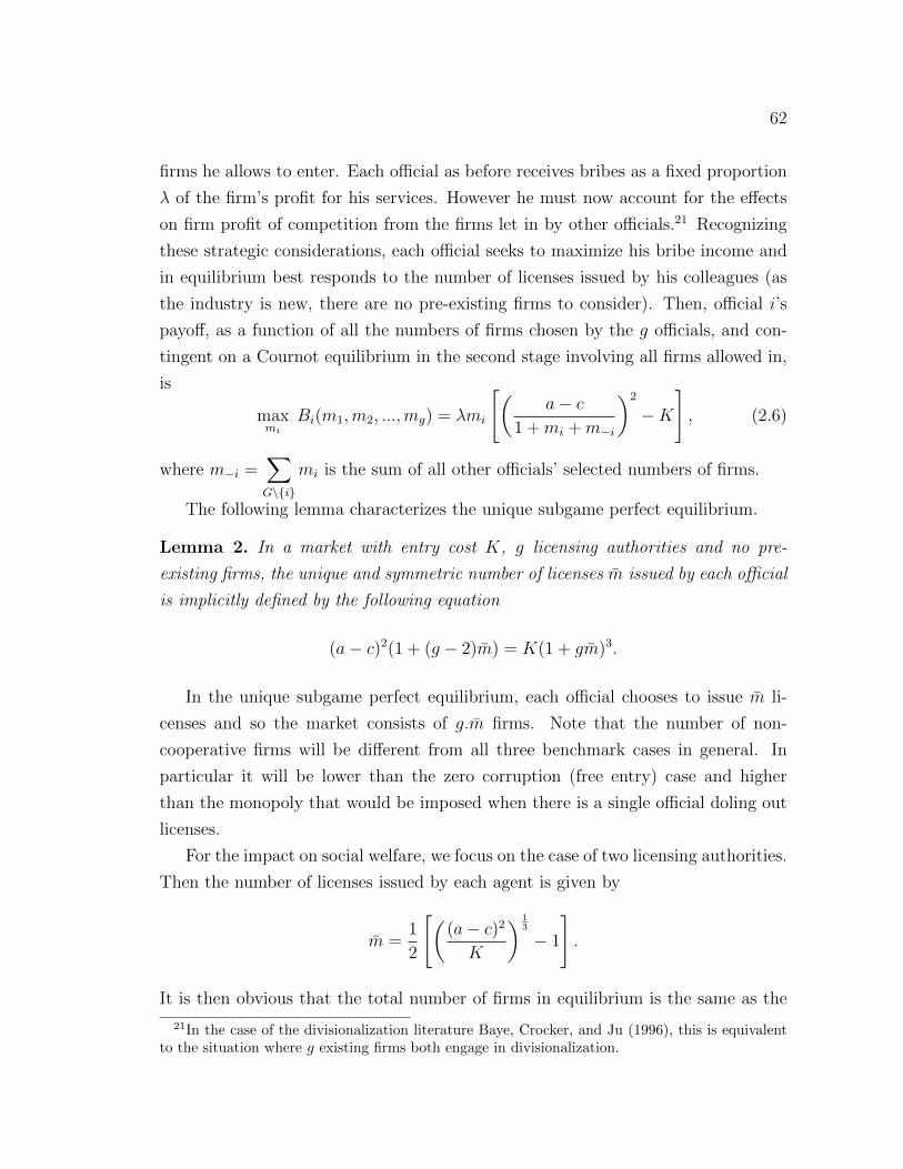
62

firms he allows to enter. Each official as before receives bribes as a fixed proportion

λ of the firm’s profit for his services. However he must now account for the effects

on firm profit of competition from the firms let in by other officials.21 Recognizing

these strategic considerations, each official seeks to maximize his bribe income and

in equilibrium best responds to the number of licenses issued by his colleagues (as

the industry is new, there are no pre-existing firms to consider). Then, official i’s

payoff, as a function of all the numbers of firms chosen by the g officials, and con-

tingent on a Cournot equilibrium in the second stage involving all firms allowed in,

is

maxmi

Bi(m1,m2, ...,mg) = λmi

[(a− c

1 +mi +m−i

)2

−K

], (2.6)

where m−i =∑G\{i}

mi is the sum of all other officials’ selected numbers of firms.

The following lemma characterizes the unique subgame perfect equilibrium.

Lemma 2. In a market with entry cost K, g licensing authorities and no pre-

existing firms, the unique and symmetric number of licenses m issued by each official

is implicitly defined by the following equation

(a− c)2(1 + (g − 2)m) = K(1 + gm)3.

In the unique subgame perfect equilibrium, each official chooses to issue m li-

censes and so the market consists of g.m firms. Note that the number of non-

cooperative firms will be different from all three benchmark cases in general. In

particular it will be lower than the zero corruption (free entry) case and higher

than the monopoly that would be imposed when there is a single official doling out

licenses.

For the impact on social welfare, we focus on the case of two licensing authorities.

Then the number of licenses issued by each agent is given by

m =1

2

[((a− c)2

K

) 13

− 1

].

It is then obvious that the total number of firms in equilibrium is the same as the

21In the case of the divisionalization literature Baye, Crocker, and Ju (1996), this is equivalentto the situation where g existing firms both engage in divisionalization.

63

second best optimal number of firms per Mankiw and Whinston (1986), i.e 2m = n∗.

The following Proposition formalizes this result and establishes the uniqueness of

the number of licensing agents that can give rise to the social optimal number of

firms.

Proposition 2. Competition among officials leads to the socially optimal number of

firms if and only if there are two independent officials in charge of issuing licenses.

To benevolent leaders of a country with known widespread corruption in govern-

ment services, the benchmark of second-best socially optimal number of firms can

only form an unattainable ideal. Yet, this simple institutional reform can actually

deliver this market ideal as a Nash equilibrium of the relevant strategic game, which

in addition does not require any form of costly monitoring or supervision. Such a

policy would be particularly beneficial in weak states where eradicating corruption

and finding ”officials of unquestioned integrity” are often fruitless endeavors, due to

political, cultural and historical factors. Once a government (or legislature) sets up

such an optimal institution, the rational forces of individual choice on the part of

all the players involved in the game yield the socially optimal outcome. In fact, the

underlying mechanism utilizes the officials’ compulsion to be corrupt for the benefit

of society, in providing a remedy to the inefficiency of the market solution to free

entry.

While the result might come as a surprise at first glance, it is actually quite intu-

itive, upon invoking known basic insights from the Cournot theory of mergers (see

Salant, Switzer and Reynolds, 1983) and divisionalization (Corchon, 1991 and Baye,

Crocker and Ju, 1996). The intuition described in the previous section pertained to

one official trading off the profit per firm allowed in and the market share of all his

firms in the total industry. With exactly two officials, the process of adjusting this

trade off creates the right incentives for the official to behave in a way compatible

with that of an honest social planner.

As discussed in more detail in a more general context in the next subsection, a

direct corollary of this result is that using three or more officials is socially subop-

timal, with welfare monotonically declining in the number of officials beyond two

(welfare is shown to be concave in the number of firms in the proofs).

The result does not depend on the value of the bribe, which can be interpreted

as one possible measure of the level of corruption. In such a case the government

64

may indeed doubly benefit, if it is the case that inter-officials competition lowers

the level of corruption. A social planner is then able to reduce both the size and

negative impact of corruption, while also avoiding the inefficiency caused by free

entry.

This solution shares one drawback with the benchmark of second-best social

optimum: They lead to market outcomes that are not entry proof. Once 2m firms

have entered, further entry remains profitable, and more firms would therefore wish

to enter. Thus, firms that have paid the bribe to enter must be guaranteed that the

officials will not allow further opportunistic rounds of entry and concomitant bribe

collection. In other words, there is an issue of credibility, some form of which is

common to most transactions under corruption. Within the two stage game model,

this issue is assumed away by construction, since officials commit to their chosen

numbers of firms in the first stage by the very structure of such games. From a

real-life point of view, such an assumption is motivated by reputational concerns on

the part of corrupt officials, a feature that is supported by anecdotal evidence.

Given the novel nature of the exercise, examples of direct application are difficult

to find. However a close example can be found in the experience of Singapore’s

custom department. Perceived as a corrupt department, the government introduced

a second (privately contracted) department with overlapping jurisdiction (Bardhan,

2006). This was done to reduce the level of corruption in the department and it is

believed it was successful in doing so. The proposition above however suggests a

more important effect of this change, the introduction of an additional official may

additionally have induced the socially optimal number of licenses to be issued.

Overall, this constitutes a novel approach of using market based mechanisms

to yield a socially optimal solution in markets characterized by two sources of in-

efficiency. This approach provides a single solution to two fundamental problems.

In one stroke it allows the social planner to avoid the disastrous consequence of a

monopoly in the market due to corruption and it also surprisingly rids the market of

inefficiency due to free entry by instituting the right amount of competition amongst

corrupt officials.

65

2.4.2 The case of a pre-existing industry

In case the industry has been in existence prior to the appointment of the current

officials, there will be some pre-existing (say `) firms operating in the market. This

feature will alter the game faced by the officials. While it is postulated here that they

will continue to charge a bribe equal to a fixed proportion of firms’ profits in period

2, they must take into consideration the effect of increased competition not only

from the firms allowed to enter by their colleagues, but also from the pre-existing

firms whom they have no control over.

In this case, official i’s payoff function (given ` pre-existing firms) is

maxmi

Bi(m1,m2, ...,mg; `) = λmi

[(a− c

1 +mi +m−i + `

)2

−K

]. (2.7)

The presence of ` pre-existing firms leads to an analytically less tractable problem

and alters the final conclusion only in a manner that goes against the conventional

wisdom on the benefits of competition in license provision in corrupt environments.

Proposition 3. In a market with pre-existing firms, the socially optimal number of

officials g∗ is either one or two, according as the existing number of firms is low or

high.

This conclusion is quite intuitive in light of the previous results of the paper. As

the proof formalizes, this conclusion rests on two key facts: (i) the final equilibrium

number of firms in the market is increasing in both the number of existing firms `

and the number of officials g, and (ii) social welfare is strictly jointly concave in the

same two variables. It follows directly from the former fact that choosing three or

more officials is never optimal, and then from the latter fact that one or two officials

might be optimal, depending on the value of `, when one keeps in mind that welfare

is maximal when there are g = 2 officials and ` = 0 existing firms (from Proposition

2).

In order to emphasize the point that monopoly in entry-certifying offices can

actually be socially optimal, we provide an explicit example.

Example. Let (a− c) = 40 and K = 1.

Short computations (with details left to the reader) establish the following compar-

isons:

66

(i) With ` = 3 pre-existing firms, welfare decreases from 780.11 with g = 2 officials

to 779.84 with g = 1 official.

(ii) With ` = 4 pre-existing firms, welfare increases from 779 with 2 officials to

782.61 with one official.

(ii) Welfare is maximized by having two officials for ` = 1, 2, 3 and one official for

` ≥ 4. In other words, g∗ = 2 for ` ≤ 3 and g∗ = 1 for ` ≥ 4

In conclusion, monopoly in entry certification is socially optimal whenever there

are at least 4 pre-existing firms in the market. Otherwise, duopoly is socially optimal.

In terms of policy prescriptions, the conclusion of this subsection is important

in a number of different dimensions. The first major implication is that the socially

optimal design for the entry certification process never calls for instituting three or

more certifying offices. From a social standpoint, the ideal ”industrial organization

of corruption” is always quite simple: Either a duopoly or a monopoly, depending

on the existing number of firms in the industry. Raising the extent of competition

amongst corrupt officials beyond duopoly is always detrimental to welfare, the more

so the further one gets from duopoly. All this would do is move the industry closer

to the free entry solution and away from the second best ideal (e.g., Mankiw and

Whinston, 1986). This conclusion is quite remarkable, particularly when one takes

into account the fact that the underlying competition is akin to Cournot, rather

than Bertrand, competition. In other words, competition proceeds not in terms of

bribe setting but rather in the ”quantities” of firms allowed in by each official. Recall

that the latter feature makes our use of competition among corrupt officials quite

distinct from what was widely envisaged in the extant literature. Nevertheless, the

conclusion that monopoly could easily emerge as the socially optimal form of entry

certification in a corrupt environment is certainly quite provocative and difficult to

anticipate on intuitive grounds.

Another implication of this result is that it cautions against the prior recommen-

dation based on the superiority of having two officials for industries with pre-existing

firms. As such, it is yet another reminder of the importance of the distinction be-

tween new and existing industries when designing optimal institutions to regulate

entry into markets when a necessary certification process must be delegated to cor-

rupt officials.

Naturally, if one were to take into account the (fixed) costs associated with

67

instituting certifying offices, the inedaquacy of oligopoly would become more pro-

nounced. In addition, the balance would tilt further in favor of having one office

instead of two, for markets with pre-existing firms.

In terms of limitations, it is fair to observe that this conclusion is predicated

on the mode of competition being in the numbers of firms as well as on the lack of

collusive behavior on the part of the officials involved. Admittedly, postulating non-

collusive behavior in this particular context is somewhat of a leap of faith. Indeed,

if these officials are assumed to operate with full impunity, they need not fear any

antitrust-like enforcement against collusive behavior. On the other hand, the social

planner will typically hold various suitable means to foster a climate of rivalry

between the competing officials. If one were to take into account the possibility of

collusive behavior, then a more diffuse industrial organization of corruption might

be to the advantage of society, simply because of the well known fact that collusion

is more difficult to sustain when more participants are involved.

2.5 Conclusion

The present paper joins a small but growing literature that adopts a positive per-

spective on market performance centered around the integration of corruption as a

key determinant of market structure. Corruption is viewed as the sale of govern-

ment property for purely selfish gain by mid-level officials, whose corrupt behavior

is limited only by the economic environment, but not by legal or ethical constraints.

The focus of the paper is on endogenous entry when firms require a license that the

official issues, but only upon charging a percentage of the firm’s profit as a bribe.

With no existing firms in the market, this scheme will always give rise to a

corruption-induced monopoly, and thus typically to drastic under entry. However,

in reality, a particular official will be faced with existing firms that are out of his reach

and may not be forced to pay a bribe. In such cases, the official’s ability to curtail

competition may be drastically reduced, and the outcome may exceed the socially

optimal number of firms. This result paves the way for some policy prescriptions

on the part of a benevolent head of government, including issuing special licenses

from his office to create or increase the number of existing firms before letting a

corrupt official take over, and timing officials’ nomination to particular industries

with a view to avoid any corruption-induced monopolies (in particular arrange for

68

the transfer of any official shortly after overseeing a new industry launch).

A benevolent leader may also delegate the authority to issue licenses to multiple

authorities, who then compete in the numbers of firms they allow in the market while

all charging the same type of bribe as before. The main result here is that, with

two officials, the outcome will be the socially optimal number of firms. This result

constitutes an extreme illustration of the theory of the second-best as envisioned

by Lipsey and Lancaster (1957): The two distortions at hand, free entry under

imperfect competition and the presence of fully corrupt officials, exactly offset each

other and yield an implementation of the second best solution, as defined by Mankiw

and Whinston (1986). With pre-existing firms in the market, the socially optimal

number of officials is always either one or two, implying a relatively simple and

realistic structure for the socially optimal industrial organization of corruption. The

latter relies on the presence of corruption, and is thus not aimed at eradicating it.

The results of the paper enlighten the much discussed relationship between com-

petition and corruption. As in Bliss and DiTella (1997), the two variables are

endogenously and simultaneously co-determined, rendering any comparative statics

perspective a rather complex issue. Nevertheless, for the discrete comparison of

entry under corruption and entry without corruption, one can conclude that cor-

ruption need not stifle competition. In fact, it may even partially or fully correct

the natural inefficiency inherent in free entry, depending on the number of initial

firms operating in the industry (Mankiw and Whinston, 1986). When no such firms

are present, corruption with two competing officials restores full (second-best) ef-

ficiency. With sufficiently many pre-existing firms, a monopoly official is socially

optimal, a rather surprising conclusion going against conventional wisdom on cor-

ruption (Rose-Ackerman, 1978). One key finding of the paper is that the number

of pre-existing firms emerges as a key parameter that may play a critical role in

this complex relationship. This realistic parameter is a priori exogenous in the basic

model, but may become endogenous as part of an active government intervention

scheme aiming at a socially efficient outcome.

Our analysis and conclusions suggest some testable implications of potential in-

terest for empirical work on corrupt economies, even though reliable data is difficult

to obtain for well known reasons, including the obvious secrecy requirements and the

developing state of most relevant economies. One testable implication is whether

a high rate of turnover of entry-certifying officials within industries with long-lived

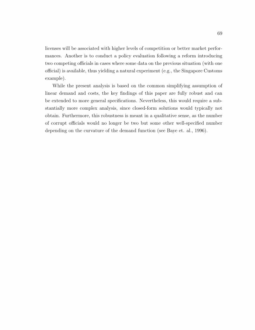
69

licenses will be associated with higher levels of competition or better market perfor-

mances. Another is to conduct a policy evaluation following a reform introducing

two competing officials in cases where some data on the previous situation (with one

official) is available, thus yielding a natural experiment (e.g., the Singapore Customs

example).

While the present analysis is based on the common simplifying assumption of

linear demand and costs, the key findings of this paper are fully robust and can

be extended to more general specifications. Nevertheless, this would require a sub-

stantially more complex analysis, since closed-form solutions would typically not

obtain. Furthermore, this robustness is meant in a qualitative sense, as the number

of corrupt officials would no longer be two but some other well-specified number

depending on the curvature of the demand function (see Baye et. al., 1996).

70

APPENDIX A

APPENDIX TO CHAPTER 1

A.1 Hedonic Regression Results

A hedonic analysis is presented here to gain an insight into the relationship between

the installation decisions and its potential factors at the zip code level. This allows

the use of household characteristics such as the income term that is left out by the

structural model.

A.1.1 Factors that Influence Investment Decisions

According to a CSI survey, consumers consider the following reasons when mak-

ing the investment in thtet solar power system- financial concern, environmental

concern and image/prestige effect. The variables that address the financial concern

include the median household income, solar power system price, CSI subsidy, federal

tax credit and the revenue generated by producing solar electricity. One potential

measure that could capture the environmental concern is to use the electric vehicle

ownership in a zip code. However, we currently don’t have access to this infor-

mation. The prestige factor is not addressed in this paper and we treat it as an

unobserved component in the error term.

• Model I

Let N be the number of adopters in a zip code z and time period t. M is the

number of owner occupied households in that zip code and Y is the median

household income among the owner occupied households in 2010 dollars. Let

N07 be the total cumulative number of adoption in that zip code prior to

the start of the CSI program. This variable can be view as the proxy that

captures many unobservables in a zip code such as the environmental attitude

or exposures to the solar rebate program due to the presence (or the lack of

it) of solar equipment retailing offices. Assuming a uniform size of 5.59kW for

each unit of system invested. Let p be the price per unit after the sales tax.

71

Let s be the total CSI EPBB subsidy, τ as the federal 30% tax credit and r

as the net present value of the electricity revenue for the next 25 years taken

out the future O&M costs.

The first regression equation that describes the potential consumer behavioras

Nzt = α0 + α1 Mz + α2 Yz + α3 N07z + α4 pzt + α5 st + α6 τt + α7 rzt + εzt (A.1)

Regression specification I-III are under this model where the first specification

is (A.1), the second specification includes the year fixed effects and the third

includes both year and utility fixed effects.

• Model II

The second model does away with the average size assumption and examinethe correlation between number of installations and per watt price (cPw), CSIsubsidy (slevel), percent of tax credit1(τ level). The revenue term is separatedinto the electricity price (ce) and solar potential (sun) in kWh/m2/day. In avariation to this model (spec 4), we used a measure of subsidy as the proportionto the price per watt (sprop).

Nzt = α0+α1 Mz+α2 Yz+α3 N07z +α4 cPwzt+α5 s

levelt +α6 τ

levelt +α7 c

et +α8 sunzt+εzt

(A.2)

Specification 4 and 5 are under the second model. The only difference is on

how the subsidy is measured, i.e. whether it’s by the dollar amount or as the

percentage discount relative to the original price. The latter addressed the

consumer behavior when they care more about the percent of discount that

they receive than the final price that they are paying. Following the classical

assumption of ordinary least square that the error term is uncorrelated across

time and zip codes. The concern for serial correlations across zip codes is

mitigated by the pre-2007 installations measure.

The regression results show that richer zip codes are more likely to have solar

installation. For each $1000 increase in the median household income, we

would expect to see 9 to 10 more units being installed. The unobserved zip

1Despite that tax credit has been set at the 30% rate during the period of 2007-2012, thereis one policy change in 2009. The original cap for the tax credit is at $2,000 and the AmericanRecovery and Reinvestment Act come in to effect on January 2009 to lift the cap. In effect, before2009 the tax credit is around 5% for a 5kW system and higher for a smaller unit.

72

code heterogeneity proxied by the pre-2007 cumulative installation number has

a significant effect on the outcome of subsequent investment choices in each zip

code. We found that for each additional unit being installed prior to 2007, we

would expect to see 0.02 more investment cases in solar power systems. This

could be explain by the peer effect discussed by [15], the environmental attitude

that is perchant to the zip code (example of the Berkeley neighborhoods) or

distance to the retailer/installer.

The reduced form results in the tax credit effect are similar to what we dis-

cussed in the structural form model that it is not well identified. It’s estimated

sign is positive and significant under the first specification and later changes

to negative and significant under the second specification. In the third specifi-

cation is negative and insignificant. The upfront system cost has the greatest

effect on the investment decision. For each $1000 increase in the system cost,

it leads to 168 to 248 less units being purchased and installed. Both solar

potential and electricity price, two crucial factors in determining the revenue

exhibits significant and large effects on the investment decisions.

73

Table A1.1 Regression results

(1) (2) (3) (4) (5)

install install install install install

# households 0.000144∗∗∗ 0.000147∗∗∗ 0.000146∗∗∗ 0.000141∗∗∗ 0.000141∗∗∗

(42.45) (42.57) (41.97) (40.86) (40.86)

income 0.00927∗∗∗ 0.00983∗∗∗ 0.0104∗∗∗ 0.0102∗∗∗ 0.0102∗∗∗

(20.20) (21.31) (22.19) (21.95) (21.96)

# pre2007 0.0243∗∗∗ 0.0239∗∗∗ 0.0241∗∗∗ 0.0242∗∗∗ 0.0242∗∗∗

(47.82) (46.56) (46.98) (47.30) (47.27)

system cost -0.168∗∗∗ -0.189∗∗∗ -0.248∗∗∗

(-22.00) (-14.79) (-16.36)

CSI subsidy 0.0692∗∗∗ 0.135∗∗∗ 0.0727∗∗∗

(8.31) (12.52) (5.42)

tax credit 0.00833∗ -0.287∗∗∗ -0.0880

(1.98) (-4.83) (-1.36)

revenue 0.404∗∗∗ 0.430∗∗∗ 0.418∗∗∗

(27.83) (28.61) (15.79)

2007 -2.909∗∗∗ 0.131 -14.02∗∗ -7.912

(-4.53) (0.17) (-2.71) (-1.61)

2008 -2.347∗∗∗ 0.557 -13.48∗∗ -7.375

(-3.72) (0.76) (-2.62) (-1.50)

2009 0.846∗∗∗ 1.323∗∗∗ 1.273∗∗∗ 1.347∗∗∗

(6.81) (9.52) (9.00) (9.61)

2010 0.657∗∗∗ 0.883∗∗∗ 0.918∗∗∗ 0.984∗∗∗

(6.79) (8.76) (9.04) (9.71)

2011 0.477∗∗∗ 0.529∗∗∗ 0.691∗∗∗ 0.716∗∗∗

(6.33) (6.99) (9.07) (9.34)

SDG&E 0.0576 -0.274∗∗∗ -0.280∗∗∗

(0.93) (-3.76) (-3.81)

SCE 0.441∗∗∗ 0.769∗∗∗ 0.802∗∗∗

(6.56) (10.64) (11.10)

cost/watt -1.623∗∗∗ -1.679∗∗∗

(-21.11) (-20.58)

subsidy % 4.405∗∗∗

(8.15)

tax credit(level) -60.52∗∗ -36.92

(-2.99) (-1.91)

elec. price 0.683∗∗∗ 0.689∗∗∗

(18.60) (18.62)

solar potential 0.408∗∗∗ 0.407∗∗∗

(5.58) (5.57)

subsidy 0.540∗∗∗

(7.21)

cons 0.745∗ 3.752∗∗∗ 4.027∗∗∗ 13.73∗ 6.953

(2.29) (7.70) (6.83) (2.19) (1.16)

N 20727 20727 20727 20727 20727

t statistics in parentheses∗ p < 0.05, ∗∗ p < 0.01, ∗∗∗ p < 0.001

74

A.2 Full Tables

Table A2.1 Summary statistics

Variable Mean Std. Dev. Min Max Obs.

System price 44,702 4,212 34,122 51,318 21,861

Capacity-based subsidy 8,083 4,516 1,398 13,975 21,861

Present value of 25-year production revenue

10%: 13,757 1,159 11,755 17,978 21,861

5%: 19,578 1,649 16,729 25,585 21,861

3%: 23,946 2,017 20,462 31,294 21,861

Present value of 25-year O&M costs

10%: 3,347 78.9 20,461 31,294 21,861

5%: 4,809 113.4 4,533 4,986 21,861

3%: 5,912 139.4 5,572 6,130 21,861

Tax credits 8,071 4,835 2000 14,193 21,861

Electricity rate (ave.) 16.06 1.02 14.8 18.68 18

PG&E: 15.77 0.57 15 16.3 6

SCE: 15.72 0.83 14.8 17.12 6

SDG&E: 17.41 1.30 15.6 18.68 6

Irradiation 5.55 0.28 5.08 6.57 21,861

Wage 1,085 120 930 1253 9

Cost per watt 7.4 0.7 5.69 8.5 21,861

# install 1.34 2.30 0 42 21,861

Table A2.2: Comparison of the average size from leased and non-leased units

(Two-sample t test with equal variances)

Group Obs Mean Std. Err. Std. Dev 95 % Conf. Interval

0 (non-leased) 50277 5590.47 32.207 7221.67 5527.35 5653.60

1 (leased) 27139 6456.40 88.27 14514.78 6283.38 6629.41

combined 77416 5894.03 37.38 10400.45 5820.77 5967.30

difference -865.93 78.28 -1019.35 -712.50

diff = mean(0) - mean(1) t=-11.06

Ho: diff = 0 degrees of freedom = 77414

Ha: diff < 0 Pr(T < t) = 0.0000

75

Table A2.3: Regression result on cost per watt and its factors

cPw t-stat

pre2007 -0.00192∗∗∗ (-11.82)

size (kW) -0.0439∗∗∗ (-42.89)

size2 (kW2) 0.0000508∗∗∗ (32.07)

wages 1.642∗∗∗ (36.59)

Module cost 0.936∗∗∗ (31.33)

2007 – omitted –

2008 0.162∗∗∗ (5.92)

2009 -0.0810∗∗ (-2.90)

2010 -0.0659 (-1.59)

2011 0.142∗ (2.25)

2012 -0.177∗ (-2.20)

PG&E – omitted –

SCE 0.688∗∗∗ (45.67)

SDG&E 0.276∗∗∗ (14.64)

cons 2.016∗∗∗ (13.03)

N 73787

∗ p < 0.05, ∗∗ p < 0.01, ∗∗∗ p < 0.001

76

Table

A2.

4:E

stim

atio

nR

esult

sfr

omM

axim

um

Lik

elih

ood

Est

imati

on

Model

Sp

ecifi

cati

ons

under

diff

eren

tdis

count

rate

s

null

III

III

IVnull

III

III

IVnull

III

III

IV

Var

iable

s10%

10%

10%

10%

10%

5%5%

5%5%

5%

3%

3%

3%

3%

3%

syst

emco

st-0

.123∗∗

∗-0

.154

8∗∗

∗-0

.279

8∗∗

∗-0

.123

8∗∗

∗-0

.153

5-0

.282

3∗∗

∗-0

.1244

-0.1

523∗∗

∗-0

.2357∗∗

∗

(0.0

151)

(0.0

220

)(0

.009

4)(0

.016

0)(0

.036

0)(0

.0166)

(0.0

274)

CSI

subsi

dy

0.04

09∗

0.08

64∗∗

∗0.0

996∗

∗∗0.

0432

∗0.

0860

0.10

23∗∗

∗0.0

455

0.0

853∗

∗∗0.1

244∗

∗∗

(0.0

165)

(0.0

187)

(0.0

104)

(0.0

173)

(0.0

151)

(0.0

136)

(0.0

131)

Rev

enue

0.10

18∗

0.0

795

0.09

59∗

0.0

735∗

0.05

92

0.0

744

0.0

668

0.0

527

0.0

707

(0.0

400

)(0

.078

4)(0

.050

0)

(0.0

334)

(0.0

584)

(0.0

492)

(0.0

631)

Tax

cred

it0.

031∗

∗∗0.

0522

∗∗∗

0.19

43∗∗

∗0.

0311

∗∗∗

0.05

120.

1915

∗0.0

309

0.0

504∗

∗∗-0

.0433

(0.0

073)

(0.0

108)

(0.0

157)

(0.0

092)

(0.0

961)

(0.0

116)

(0.0

376)

Net

cost

-0.1

706∗∗

∗-0

.1575∗∗

∗-0

.1485∗∗

∗

(0.0

161)

(0.0

178)

(0.0

166)

Y20

072.

4173

∗∗∗

0.20

21

2.42

32∗

0.2

209

-0.2

636

0.2

109

(0.0

348)

(0.1

655)

(1.0

835)

(0.1

883)

(0.4

043)

(0.1

599)

Y200

82.

9774

∗∗∗

0.93

38∗∗

∗2.

9929∗

∗0.9

359∗

∗∗0.3

566

0.9

117∗

∗∗

(0.0

339)

(0.1

966)

(1.0

723)

(0.2

226)

(0.3

799)

(0.2

033)

Y200

91.

0151

∗∗∗

-0.4

947∗∗

∗1.

042

7∗∗∗

-0.4

576∗∗

∗1.0

785∗∗

∗-0

.4419∗∗

∗

(0.1

296)

(0.0

621)

(0.1

700)

(0.0

562)

(0.1

674)

(0.0

448)

Y201

00.

7952

∗∗∗

-0.0

849

0.82

14∗∗

∗0.0

618

0.8

757∗∗

∗-0

.0559

(0.1

037)

(0.0

712)

(0.1

201)

(0.0

630)

(0.1

171)

(0.0

573)

Y20

110.

4133

∗∗∗

0.13

69∗∗

0.43

12∗∗

∗0.1

539∗

∗0.4

683∗∗

∗0.1

569∗∗

∗

(0.0

548)

(0.0

444)

(0.0

610)

(0.0

466)

(0.0

540)

(0.0

436)

SC

E-0

.340

7∗∗

-0.1

834

-0.7

517∗

∗∗-0

.357

30.

199

4-0

.7964∗

∗∗-0

.3664∗∗

-0.2

765

-0.8

092∗

∗∗

(0.1

129)

(0.1

202

)(0

.109

0)(0

.139

2)(0

.1150)

(0.1

415)

(0.1

552)

(0.1

456)

SD

G&

E0.

0781

0.1

303

-0.1

441

0.07

760.

1196

-0.2

721∗

0.0

866

0.1

02

-0.3

248∗

(0.1

719)

(0.6

903)

(0.1

290)

(0.2

050)

(0.1

180)

(0.2

448)

(0.2

463)

(0.1

605)

const

ant

-8.4

040

-4.5

518∗∗

∗-3

.403

8∗

-0.7

442∗∗

∗-5

.211

7∗∗

∗-8

.371

2-4

.564

7∗∗

∗-3

.477

9-0

.755

9-6

.1794∗

∗∗-8

.3383

-4.5

987

-3.5

217∗

∗-0

.2214

-6.7

065∗

∗∗

(0.7

148

)(1

.354

6)(0

.130

7)(0

.249

5)(0

.907

9)(1

.464

6)(0

.1708)

(1.2

967)

(1.8

019)

(0.1

356)

com

puti

ng

tim

e(m

ins)

1215

519

766

025

516

177

428

994

421

34

333

470

1370

534

Nob

serv

atio

ns

2186

121

861

2186

121

861

2186

121

861

2186

121861

21861

21861

21861

21861

Log

Lik

elih

ood

-264

894

-261

397

-261

171

-260

689

-261

174

-2648

94-2

6140

3-2

6118

3-2

6068

7-2

61188

-264894

-261405

-261195

-260712

-261207

LR

chi2

6995

744

784

1074

4069

8274

2284

157412

6977

7398

8364

7376

pro

b>

chi2

00

00

00

00

00

00

Pse

udoR

21.3

2E-0

21.

41E

-02

1.59

E-0

21.

40E

-02

1.32

E-0

21.

40E

-02

1.59E

-02

1.4

0E

-02

1.3

2E

-02

1.4

0E

-02

1.5

8E

-02

1.3

9E

-02

standar

der

rors

inpar

enth

eses

∗p<

0.05

,∗∗p<

0.01,

∗∗∗p<

0.0

01

77

Table A2.5: Welfare analysis of current subsidy programs

Without subsidies With current subsidies

10%

Purchase probability 2.82e-05 to 1.02e-04 2.93e-04 to 6.8e-04

# first month adopter 113 825

Change in purchase prob. 84-90%

Subsidy amount 11k - 14k

Government Spending $948 millions

Change in CS $418 millions

Implied CO2 price (/ton)

SCE $121 (0.76)

PG&E $105 (0.35)

SDG&E $100 (0.12)

Overall $107 (0.40)

5%

Purchase probability 3.43e-05 to 1.42e-04 2.86e-04 to 7.4e-04

# first month adopter 136 815

Change in purchase prob. 80-88%

Subsidy amount 11k - 14k

Government Spending $2.23 B

Change in CS $1.09 B

Implied CO2 price

SCE $116 (0.78)

PG&E $101 (0.35)

SDG&E $95 (0.12)

Overall $103 (0.40)

3%

Purchase probability 3.23e-05 to 1.7e-04 2.87e-04 to 7.59e-04

# first month adopter 159 816

Change in purchase prob. 77-86%

Subsidy amount 11k - 14k

Government Spending $3.30 billions

Change in CS $1.79 billions

Implied CO2 price

SCE $109 (0.79)

PG&E $94 (0.34)

SDG&E $88 (0.12)

Overall $96 (0.40)

All dollar values are in 2012 dollar. Standard errors to the prices are shown in bracket. The unit, ton, used in this paper refers to metric ton.

78

Table A2.6: Counterfactual with solar irradiation for Frankfur, Germany

Baseline Frankfurt irradiation Frankfurt irradiation/

same num. installations

Frankfurt irradiation/

same electricity prod.

10% + $6,800 + $11,200

Change in purchase prob. 84-90% 84-91% 95-97% 97-99%

Total Installations 776,486 292,342 773,313 1,256,789

Installations due to subsidy 646,307 250,355 731,326 1,214,802

Total electricity production 16.5 TWh 2.4 TWh 8.4 TWh 16.5 TWh

Upfront subsidy 11k - 14k 11k - 14k 18k-21k 22k-25k

Government spending 948 million 310 million 1.47 billion 3.55 billion

Change in CS 418 million 134 million 459 million 952 million

add. CO2 displaced 4.9 MMt 0.84 MMt 2.8 MMt 5.6 MMt

CO2 price (per ton) $107 (0.40) $209 (0.72) $362 (0.84) $461 (1.05)

5% + $10,100 + $15,700

Change in purchase prob. 82-89% 82-89% 96-98% 98-99%

Total Installations 775,854 205,023 772,698 1,298,345

Installations due to subsidy 617,585 171,145 738,820 1,264,467

Total electricity production 38.8 TWh 4 TWh 19 TWh 38.6TWh

Upfront subsidy 11k - 14k 11k - 14k 21k - 24k 27k - 30k

Government spending 2.2 billion 522 million 4.1 billion 9.9 billion

Change in CS 1.1 billion 241 million 1.25 billion 2.7 billion

add. CO2 displaced 11 MMt 1.4 MMt 6.6 MMt 13 MMt

CO2 price (per ton) $103 (0.40) $203 (0.70) $422 (1.03) $544 (1.08)

3% + $12,400 + $19,200

Change in purchase prob. 77-86% 80-87% 96-98% 98-99%

Total Installations 777,180 171,508 777,274 1,334,322

Installations due to subsidy 593,482 140,078 745,843 1,303,891

Total electricity production 57 TWh 5.978 TWh 29.5 TWh 57 TWh

Upfront subsidy 10,942-13,892 10,942-13,892 23,342-26,292 30,142-33,092

Government spending 3.3 billion 0.7 billion 6.7 billion 16.5 billion

Change in CS 1.8 billion 0.3 billion 2.1 billion 4.9 billion

add. CO2 displaced 15.7 MMt 1.7 MMt 10 MMt 19.5 MMt

CO2 price (per ton) $96 (0.40) $193 (0.69) $457 (1.00) $596 (1.17)

MMt refers to million metric tons

79

Table A2.7: Welfare comparison between capacity-based and production-based subsidies

Baseline Feed-in Tariff Baseline with NJ irradia-

tion in N. CA

FIT with greater disparity

between north and south

10% FIT=15.345/kWh FIT=15.71/kWh

Change in purchase prob. 84-90% 84-91% 84-90% 82-92%

Total Installations 776,486 770,797 685,614 670,066

Installations due to subsidy 646,307 640,619 574,540 558,992

Total electricity production 16.5 TWh 16.6 TWh 13.7 TWh 13,782

Per unit Subsidy 11k-14k 10874-14134 11k-14k 10376-14,723

Government spending 948 million 949 million 824 million 824 million

Change in CS 418 million 420 million 360 million 361 million

add. CO2 displaced 4.9 MMt 5 MMt 4 MMt 4 MMt

CO2 price (per ton) $107.25 (0.40) $106.58 (0.05) $112.96 (0.45) $111.86 (0.07)

5% FIT=9.8/kWh FIT=10.225/kWh

Change in purchase prob. 82-89% 81-88% 81-88% 79-89%

Total Installations 775,854 772,825 686,796 674,534

Installations due to subsidy 617,585 614,555 551,167 538,904

Total electricity production 38.8 TWh 38.9 TWh 32.7 TWh 32.8 TWh

Per unit Subsidy 11-14k 10930-14136 11k-14k 10,394- 14,749

Government spending 2.227 billion 2.232 billion 1.96 billion 1.96 billion

Change in CS 1.1 billion 1.1 billion 951 million 957.5 million

add. CO2 displaced 11 MMt 11 MMt 9.4 MMt 9.4 MMt

CO2 price (per ton) $102.7 (0.40) $102.12 (0.04) $108 (0.46) $107 (0.11)

3% FIT=8.025/kWh FIT=8.375/kWh

Change in purchase prob. 77-86% 78-85% 77-86% 77-86%

Total Installations 777,180 774,940 680,368 670,651

Installations due to subsidy 593,482 591,241 525,110 515,394

Total electricity production 57.43 TWh 57.46 TWh 48.02 TWh 48.12 TWh

Per unit Subsidy 10,942-13,892 10,947-14,158 10,942-13,892 10,419-14,784

Government spending 3.3 billion 3.3 billion 2.88 billion 2.89 billion

Change in CS 1.8 billion 1.8 billion 1.55 billion 1.56 billion

add. CO2 displaced 15.7 MMt 15.7 MMt 13.2 MMt 13.2 MMt

CO2 price (per ton) $96.06 (0.40) $95.47 (0.05) $101.09 (0.45) $100.13 (0.11)

Table A2.8: Potential impact of the pending tariff on imported Chinese solar cells

10% increase 25% increase

in module price in module price

10% discount rate

Increase in system price 2.61% to 3.45% 6.52% to 8.63%

# reduction in first month 129 293

% change in installations -15.64% -35.56%

5% discount rate

Increase in system price 2.61% to 3.45% 6.52% to 8.63%

# reduction in first month 114 265

% change in installations -13.84% -32.08%

3% discount rate

Increase in system price 2.61% to 3.45% 6.52% to 8.63%

# reduction in first month 103 243

% change in installations -12.48% -29.36%

All dollar values are in 2012 dollar

80

Table A2.9: Potential impacts from varying incentive levels

Current Lowering subsidy Doubling num.

Subsidy level match $21 SSC of installations

10%

Change in purchase prob. (from

baseline)

84-90% 38% 95-96%

Total Installations 776,486 204,600 1,556,341

Installations due to subsidy 646,307 74,422 1,426,163

Total electricity production 17 TWh 4 TWh 48 TWh

Upfront subsidy 11k-14k 2.8k 19.3k

Government spending 948 million 50 million 4.5 billion

Change in CS 418 million 40 million 1.5 billion

add. CO2 displaced 5 MMt 0.5 MMt 16 MMt

Equivalent CO2 price $107 (0.40) $21 (0.04) $187 (0.41)

5%

Change in purchase prob. 80-88% 36-37% 94-95%

Total Installations 775,854 244,741 1,556,710

Installations due to subsidy 617,585 86,472 1,398,441

Total electricity production 39 TWh 11 TWh 101 TWh

Upfront subsidy 11k-14k 3k 20.7k

Government spending 2.2 billion 158 million 10 billion

Change in CS 1.1 billion 128 million 3.9 billion

add. CO2 displaced 11 MMt 1.4 MMt 33 MMt

Equivalent CO2 price $103 (0.40) $21 (0.04) $187 (0.46)

3%

Change in purchase prob. 77-86% 37-39% 92-95%

Total Installations 777,180 288,560 1,554,408

Installations due to subsidy 593,482 104,901 1,370,709

Total electricity production 57 TWh 20 TWh 126 TWh

Upfront subsidy 11k-14k 3.4k 22k

Government spending 3.3 billion 322 million 14.6 billion

Change in CS 1.8 billion 270 million 6.5 billioin

add. CO2 displaced 15.7 MMt 2.6 MMt 44 MMt

Equivalent CO2 price $96 (0.40) $21 (0.04) $186 (0.48)

All dollar values are in 2012 dollar

81

A.3 Calculating the equivalent CO2 prices from deadweightloss

The deadweight loss (DL) can be derived by subtracting the increase in consumer

surplus (CS) due to the increase in subsidy from the total government spending on

subsidy (G).

DL = G−4CS

In the logit models, consumer surplus at the specified state (S) is the logit inclusive

value and θ.

CS(S) =1

θlog(eβEV (S) + eν(S)

)×M (A.3)

Let M denote the market size, S as the current subsidy amount. Since the consumers

are forward looking in the infinite horizon time span, we need to forward simulate the

government spending in a very long horizon (H), take 100 years for example. The

purchase probability stays constant in each period during the forward simulation

process, however the market size changes due to installers exiting the market. Let

nzt be the number of adopters in each zip code, z at time period (month) t. The

net present value of the total program spending can be expressed as

G = (1 β β2 · · · β12·H)

n11 n12 · · ·n1H·12

......

......

...

nz1 nz2 · · ·nzH·12

︸ ︷︷ ︸

zipcode×12·H

· S

′

, (A.4)

and the change in consumer surplus as (where S0 is the pre-policy change subsidy

amount)

4CS = CS(S)− CS(S0). (A.5)

The change in the number of installations due to the change in subsidy amount is

4Q =12·H∑h=1

[Qh(S)−Qh(S0)] . (A.6)

82

Finally the implied CO2 price can be derived as the loss in surplus per unit of CO2

displaced or formally as

PCO2 =G−4CSγ ×4Q

. (A.7)

γ is a constant which represents the amount of CO2 displaced due to the avoided

electricity generation from the fossil fuel based power plant. The average CO2 emis-

sion associated with each unit of electricity production is taken from the California

Air Resources Board report. Average amount of CO2 emission associated with each

MWh of electricity generation is 0.348 ton. Take San Diego vicinity for example,

γ = 73 ton/unit which means by installing a solar power system with the average

size of 5.59 kW, the system owner reduced the carbon dioxide emission by 73 tons

over the 25 year lifetime of the system.

A.4 Parameter Calibration and Data Cleaning

Table A4.1 Overall component DC-AC derate factor

Component Derate Factors Rate

PV Module nameplate DC rating 0.95

Inverter and Transformer 0.92

Diodes and connections 0.99

DC wiring 0.98

AC wiring 0.99

Soiling 0.95

System availability 0.98

Overall DC-AC derate factor 0.78

Assumption based on 25°C, no shading

Table A4.2 Assumptions in simulating the future revenue and costs

Inflation 1.20%

Annual O& M and insurance cost $250

Inverter Replacements Twice (8th and 17th year, 70/W)

Utility Electric rate escalation 1.09%

Demand rate escalation 0%

Photovoltaic degradation factor (per year) 0.8%

83

A.5 On Deriving the Logit Inclusive Value

From (1.5), the expected future utility function is

Fθ(X) =

∫X′

∫ε′

[maxd

[ν(X′, d, θ) + βFθ(X) + ε(d)]]pε(ε

′|X)dε′ · pX(X′|X)dX′.

(A.8a)

or

Fθ(X) =

∫X′Eε

[maxd

[ν(X′, d, θ) + βFθ(X′) + ε(d)]]pX(X′|X)dX′. (A.8b)

Since ε follows type I extreme value distribution,

Gε(y) = ee− y−ba = e−ke

− ya (A.9a)

and

gε(y) =k

ae−

ya e−ke

− ya (A.9b)

for k = ba. The distribution function of max

d=0,1Ui = max

d=0,1[vθ(X, d) + ε(d)] is equal to

H(y) =1∏d=0

Fε (y − vθ(X, d))

=∏

d={0,1}

e−ke− y−vθ(X,d)a

= e−kLe−xa .

(A.10)

where L =∑

d={0,1}evθ(X,d)

a . The corresponding pdf is

h(y) =kL

ae−

ya e−kLe

− ya (A.11)

84

The expected value of the maximum, i.e. Eε′

[maxd={0,1}

vθ(X, d) + ε(d)

]can be written

as ∫ ∞−∞

y h(y)dy

=

∫ ∞−∞

y · kLaeya e−kLe

− ya dy.

(A.12)

Let t = e−ya or −a ln t = y ⇒ dt = − 1

ae−

ya , using a change of variables (A.12) can

be solved by applying the Laplace transformation∫∞

0e−st ln tdt = − ln s+r

s,∫ 0

∞akL ln t e−kLtdt

=akLln kL+ r

kL

=ar + a(ln k + lnL)

=ar + a(b

a) + a lnL

=a ln1∑d=0

evθ(X,d)

a

(A.13)

the last equality is hold by the mean zero assumption, ar + b = 0. Therefore the

expected future utility is

F (X) =

∫X′a ln

1∑d=0

evθ(X,d)

a pX(X′|X)dX′

=

∫X′a ln

1∑d=0

eν(X′,d,θ)+βEV (X′)

a pX(X′|X)dX′

(A.14)

A.6 Figures and Charts

85

Figure A.1: Grid-tied cumulative PV installed capacity in California, 1996-2006

Figure A.2: Average module cost, 1975-2012

86

Figure A.3: Average install system cost in the US, 1998-2012. Source: SEIA Solar EnergyFacts: Q3 2012

Figure A.4: CSI 10 step subsidy schedule

87

Figure A.5: Subsidy degression in terms of cumulative installed capacity

88

Figure A.6: Zip code map showing PV system adoptions in California. Yellow indicatesinstallations occurred in 2011, green indicates installations in 2010.

89

Figure A.7: Map showing the counties included in the study

Figure A.8: Raw CSI installation data

90

Figure A.9: 2010 benchmark residential PV system price components, Goodrich et al.,2012

91

Figure A.10: PV system size distribution

Figure A.11: CSI subsidy by IOU territories

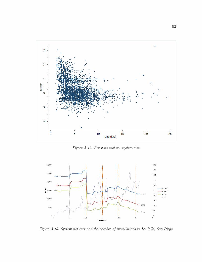
92

Figure A.12: Per watt cost vs. system size

Figure A.13: System net cost and the number of installations in La Jolla, San Diego

93

APPENDIX B

APPENDIX TO CHAPTER 2

This appendix contains the proofs of all the results of the paper, given in the same

order as in the text. For the sake of brevity, most of the computational details are

left to the interested reader.

B.1 Proof of Lemma 1

We first show that the objective function B(m; `) is a strictly quasi-concave function

of m. To this end, it is sufficient to show that the second derivative of B(m; `) is

strictly negative whenever the first derivative vanishes. To shorten notation, let

A := (a− c)2 and set λ = 1 w.l.o.g.

The first derivative of B(m; `) is

∂B(m; `)

∂m=

A

(1 + `+m)2−K − 2mA

(1 + `+m)3(B.1)

and the second derivative is

∂2B(m; `)

∂m2=

−4A

(1 + `+m)3+

6mA

(1 + `+m)4. (B.2)

Now consider

∂2B(m;`)∂m2

∣∣∣∂B`(m)/∂m=0

=−4A

(1 + `+m)3+

3A

(1 + `+m)3− 3K

1 + `+m

=−A

(1 + `+m)3− 3K

1 + `+m< 0

Hence B(m; `) is strictly quasi-concave in m. It follows that B(m; `) has a unique

argmax.

To guarantee the interiority of the maximum of B(m; `), it is sufficient to show

that its derivative is (strictly) positive at the left boundary (m = 0). In other words,

94

∂B(m; `)

∂m

∣∣∣∣m=0

=A

(1 + `)2−K > 0

since (by assumption) ` <√

AK−1, i.e., that the number of pre-existing firms is less

than the number of firms under free-entry.

To show that m ∈ [0, 1+`) when K > 0, it is sufficient to show that the derivative

of B(m; `) is strictly negative at m = 1 + `, i.e., that

∂B(m; `)

∂m

∣∣∣∣m=1+`

=A

(2(1 + `))2 −K −2(1 + `)A

(2(1 + `))3 = −K < 0.

Therefore, we always have m < 1 + `.

Finally, when K = 0, we have ∂B(m;`)∂m

∣∣∣m=1+`

= 0, so that (by the strict quasi-

concavity of B(m; `)) m = 1 + ` is the unique solution.

B.2 Proof of Proposition 1

Since (2.5) amounts to finding the zeros of a third-degree polynomial, solving yields

two complex roots and one real root. It can be verified that the unique real root is

m(`) =

(AK)13 ·[9L+

√3(A+27KL2)

K

] 23

− 313A

23

(3K)23 ·[9L+

√3(A+27KL2)

K

] 13

− L, for K > 0 (B.3)

where A = (a− c)2 and L = 1 + `. Let G(`) := `+m(`). It is easy to see that G(`)

is a continuous and strictly increasing function in ` since

G′(`) = 1+

313AK

(9 + 54

√3L

2

√A+27KL2

K

)9

[AK2

(9L+

√3(A+27KL2

K

)] 23

+

323A2K2

(9 + 54

√3L

2

√A+27KL2

K

)9

[AK2

(9L+

√3(A+27KL2

K

)] 43

−1 > 0

Recall that n = 1 ≤ n∗ ≤ n, and observe that n = 1 = G(0) < G(n) = n (the

latter inequality being due to the fact that m(n) = 0 by definition of n). Hence, by

the intermediate value theorem and the continuity and strict monotonicity of the

function G(`), there exists a unique (real number) `∗ such that G(`∗) = n∗.

95

The second part follows directly from the strict monotonicity of the function

G(`).

B.3 Proof of Lemma 2

The first-order condition in (2.6) reduces to

A(1−mi +m−i)

(1 +mi +m−i)3= K. (B.4)

This implicitly defines a reaction function mi = r(m−i), which is the same func-

tion for all players by symmetry. By differentiating and collecting terms, one can

easily check that r′i(m−i) > −1, so that the function mi + ri(m−i) is increasing in

mi. By a well known argument (see Amir and Lambson, 2000), this property implies

that no asymmetric equilibrium in the mi’s is possible.

Hence, we can assume symmetry, i.e. m−ig−1

= mi := m and simplify (B.4) to

obtain

A [1 + (g − 2)m] = (1 + gm)3K. (B.5)

Solving yields two complex roots and one real root, the latter being

m =(AKg)

13

(9 +

√3(27Kg+8A−Ag3+6Ag2−12Ag)

Kg

) 23

+ 313A

23 (g − 2)

323 g[K2g2

(9 +

√3(27Kg+8A−Ag3+6Ag2−12Ag)

Kg

)] 13

− 1

gfor K > 0

(B.6)

This completes the proof of Lemma 2.

Proof of Proposition 2

Assuming that there are g identical corrupt officials, where i chooses mi firms to

enter the market, the social welfare function is defined as (where π∗ is the profit per

firm)

W (g,m) =

g∑i=1

miπ∗ +

Q∗∫0

[P (Q)− P (Q∗)] dQ.

96

Substituting in the equilibrium profit and output from the second stage, we find

W (g,m) =

(g∑i=1

mi

)[(a− c)2

(1 +∑g

i=1 mi)2−K

]+

1

2

[(a− c)

∑gi=1mi

1 +∑g

i=1 mi

]2

.

Denoting the total number of firms in the market as n =∑g

i=1mi, welfare can be

written as

W (n) = n

[(a− c)2

(1 + n)2−K

]+

1

2

[(a− c)n

1 + n

]2

(B.7)

Differentiate (B.7) with respect to the number of firms n to get

W ′(n) =(a− c)2 −K (1 + n)3

(1 + n)3 = 0. (B.8)

The second order condition W ′′(n) < 0 is easily seen to hold, so welfare is strictly

concave in the total number of firms in the market. By symmetry, the socially

optimal number of firms let in by each official satisfies m∗ = n/g, and (B.8) yields

m∗(g) =1

g

[((a− c)2

K

) 13

− 1

]. (B.9)

Comparing (B.9) with (B.5), we have m = m∗ if and only if g = 2. Therefore

allowing exactly two officials to certify entry produces the socially optimal number

of firms in the market.

B.4 Proof of Proposition 3

The first order condition of (2.7) reduces to (with A := (a− c)2)

A(1 + `+m−i −mi)

(1 + `+mi +m−i)3= K.

With the same argument as in the proof of Lemma 2, one can rule out asymmetric

equilibria in the mi’s. Given symmetry, i.e. letting m−ig−1

= mi := m, and simplifying

yields

A[1 + `+ (g − 2)m] = K(1 + `+ gm)3. (B.10)

For clarity, denote the solution to (B.10) with its explicit arguments as m(`, g).

97

Let N(`, g) := ` + gm(`, g) denote the equilibrium total number of firms in the

market. We first show that N(`, g) is stricly increasing in both ` and g.

To this end, standard comparative statics on (B.10) with respect to ` (i.e. dif-

ferentiating once w.r.t. `) yields

∂m(`, g)

∂`=

A− 3K(1 + `+ gm)2

3Kg(1 + `+ gm)2 − A(g − 2)(B.11)

Via routine calculations, it is easy to check that ∂m(`,g)∂`

> −1g. Hence ∂N(`,g)

∂`=

1 + g ∂m(`,g)∂`

> 0.

Next, differentiating (B.10) once w.r.t. g yields

∂m(`, g)

∂g=

Am− 3Km(1 + `+ gm)2

3Kg(1 + `+ gm)2 − A(g − 2)

As before, it is easy to check that ∂m(`,g)∂g

> − mg

. Hence ∂N(`,g)∂g

= m+ g ∂m(`,g)∂g

> 0.

Hence we have shown that the final number of firms N(`, g) is stricly increasing in

both ` and g. We next make use of this result to finish the proof of the Proposition.

Social welfare is given by

W = (`+mg)

[A

(1 + `+mg)2−K

]+

1

2A

[`+mg

1 + `+mg

]2

.

Recall (from Proposition 2) that welfare is maximal when ` = 0 and g = 2, i.e.

when a total of 2m(0, 2) firms are in the market. As welfare is strictly concave in

the number of firms N = `+mg (as in the previous proof), it is also clearly strictly

concave jointly in the pair (`, g). Therefore, since N(`, g) is stricly increasing in

both ` and g, we can conclude that when ` > 0, welfare is maximized by having

either g = 2 or g = 1, according as ` is low or high.

98

REFERENCES

[1] Acemoglu, D. and T. Verdier (2000). The Choice between Market Failures andCorruption. American Economic Review, 90, pp. 194–211.

[2] Ahmad, H. and R. Burguet (2012). Institutionalising Bribery. Working Paper.

[3] Aidt, T. S. (2003). Economic analysis of corruption: a survey*. The EconomicJournal, 113(491), pp. F632–F652.

[4] Amir, R. and V. Lambson (2000). On the Effects of Entry in Cournot Markets.Review of Economic Studies, 67(2), pp. 235–254. ISSN 1467-937X.

[5] Anderson, S., A. de Palma, and J.-F. Thisse (1992). Discrete Choice Theory ofProduct Differentiation. The MIT Press.

[6] Aquirregabiria, V. and P. Mira (2010). Dynamic discrete choice structuralmodels: A survey. Journal of Econometrics, 156, pp. 38–67.

[7] Arrow, K. J., M. L. Cropper, C. Gollier, B. Groom, G. M. Heal, R. G. Newell,W. D. Nordhaus, R. S. Pindyck, W. A. Pizer, P. R. Portney, T. Sterner, R. S. J.Tol, and M. L. Weitzman (2013). How Should Benefits and Costs Be Discountedin an Intergenerational Context?

[8] Banerjee, A. V. (1997). A Theory of Misgovernance. The Quarterly Journal ofEconomics, 112(4), pp. 1289–1332. doi:10.1162/003355300555484.

[9] Barbose, G., N. Darghouth, R. Wiser, and J. Seel (2011). Tracking the SunIV: An Historical Summary of the Installed Cost of Photovoltaics in the UnitedStates from 1998 to 2010. Technical report, Lawrence Berkeley National Lab-oratory.

[10] Bardhan, P. (2006). The Economists Approach to the Problem of Corruption.World Development, 34, pp. 341–348.

[11] Baye, M. R., K. J. Crocker, and J. Ju (1996). Divisionalization, Franchising, andDivestiture Incentives in Oligopoly. The American Economic Review, 86(1),pp. pp. 223–236. ISSN 00028282.

[12] Beck, P. J. and M. W. Maher (1986). A comparison of bribery and bidding inthin markets. Economics Letters, 20(1), pp. 1 – 5. ISSN 0165-1765.

[13] Berry, S., J. Levinsohn, and A. Pakes (1995). Automobile Prices in MarketEquilibrium. Econometrica, 63, pp. 841–890.

99

[14] Bliss, C. and R. Di Tella (1997). Does Competition Kill Corruption. TheJournal of Political Economy, 105, pp. 1001–1023.

[15] Bollinger, B. and K. Gillingham (2012). Peer Effects in the Diffusion of SolarPhotovoltaic Panels. Marketing Science.

[16] Borenstein, S. (2007). Electricity Rate Structures and the Economics of SolarPV: Could Mandatory Time-of-Use Rates Undermine Californias Solar Photo-voltaic Subsidies?

[17] Borenstein, S. (2008). The Market Value and Cost of Solar Photovoltaic Elec-tricity Production.

[18] Borenstein, S. (2011). The Private and Public Economics of Renewable Elec-tricity Generation.

[19] Brattle Group, Inc., T. (2012). The Employment Impacts of Proposed Tariffson Chinese Manufactured Photovoltaic Cells and Modules. Technical report,Coalition for Affordable Solar Energy. Mark Berkman Lisa Cameron JudyChang.

[20] Burguet, R. and Y.-K. Che (2004). Competitive Procurement with Corruption.The RAND Journal of Economics, 35(1), pp. pp. 50–68. ISSN 07416261.

[21] California Energy Commission (2013). California Renewable Energy Overviewand Programs.

[22] CBO (2012). Federal Financial Support for the Development and Production ofFuels and Energy Technologies. Technical report, Congressional Budget Office.

[23] Choi, J. P. and M. Thum (2003). The dynamics of corruption with the ratcheteffect. Journal of Public Economics, 87, pp. 427–443.

[24] Choi, J. P. and M. Thum (2005). Corruption And The Shadow Economy.International Economic Review, 46, pp. 817–836.

[25] Clark, D. J. and C. Riis (2000). Allocation efficiency in a competitive briberygame. Journal of Economic Behavior and Organization, 42(1), pp. 109 – 124.ISSN 0167-2681.

[26] Corchon, L. (1991). Oligopolistic competition among groups. Economic Letters,36, pp. 1–3.

[27] Dastrup, S. R., J. G. Zivin, D. L. Costa, and M. E. Kahn (2012). Understandingthe Solar Home price premium: Electricity generation and Green social status.European Economic Review, 56, pp. 961–973.

100

[28] Dewees, D. N. (1983). Instrument choice in environmental policy. EconomicInquiry, 21, pp. 53–71.

[29] EIA (2011). Direct Federal Financial Interventions and Subsidies in Energy inFiscal Year 2010. Technical report, U.S. Energy Information Administration.

[30] EIA (2012). Annual Energy Outlook 2012. Technical report, U.S. EnergyInformation Administration.

[31] EIA (2012). Most states have Renewable Portfolio Standards.

[32] EnerNex Corp (2010). Eastern Wind Integration and Transmission Study. Tech-nical Report NREL/SR-550-47078, National Renewable Energy Laboratory.

[33] Fischer, C. and R. G. Newell (2008). Environmental and technology policiesfor climate mitigation. Journal of Environmental Economics and Management,55, p. 142162.

[34] GE Energy (2010). Western Wind and Solar Integration Study. TechnicalReport NREL/SR-550-47434, National Renewable Energy Laboratory.

[35] Goodrich, A., T. James, and M. Woodhouse (2012). Residential, Commercial,and Utility-Scale Photovoltaic (PV) System Prices in the United States: Cur-rent Drivers and Cost-Reduction Opportunities. Technical Report NREL/TP-6A20-53347, National Renewable Energy Laboratory.

[36] Goulder, L. and I. W. H. Parry (2008). Instrument Choice in EnvironmentalPolicy. Review of Environmental Economics and Policy, 2, pp. 152–174.

[37] Goulder, L. H., I. W. H. Parry, R. C. W. III, and D. Burtraw (1998). TheCost-Effectiveness of Alternative Instruments for Environmental Protection ina Second-Best Setting.

[38] Gowrisankaran, G., S. Reynolds, and M. Samano (2011). Intermittency andthe Value of Renewable Energy.

[39] Greenstone, M., E. Kopitz, and A. Wolverton (2011). ESTIMATING THE SO-CIAL COST OF CARBON FOR USE IN U.S. FEDERAL RULEMAKINGS:A SUMMARY AND INTERPRETATION.

[40] Hand, M., S. Baldwin, E. DeMeo, J. Reilly, T. Mai, D. Arent, G. Porro,M. Meshek, and D. Sandor (2012). Renewable Electricity Futures Study. Tech-nical report, National Renewable Energy Laboratory.

[41] IEA (2012). World Energy Outlook 2012. International Energy Agency.

101

[42] Jain, A. K. (1999). Models Of Corruption. In Jain, A. K., W. J. Samuels,and W. Darity (eds.) Economics of Corruption, volume 65 of Recent EconomicThought Series, pp. 13–34. Springer US. ISBN 978-1-4615-4935-2.

[43] Jain, A. K. (2001). Corruption: A Review. Journal of Economic Surveys,15(1), pp. 71–121. ISSN 1467-6419. doi:10.1111/1467-6419.00133.

[44] Johnson, L. and C. Hope (2012). The social cost of carbon in U.S. regulatoryimpact analyses: an introduction and critique. Journal of Envrieonmental StudyScience, 2, pp. 205–221.

[45] Keohane, N. O., R. Revesz, and R. Stavins (1998). The Choice of RegulatoryInstruments in Environmental Policy. Havard Environmental Law Review, 22,pp. 313–367.

[46] Kneese, A. and B. Bower (1968). Managing Water Quality: Economics, Tech-nology, Institutions. Johns Hopkins Press.

[47] Lien, D.-H. D. (1986). A note on competitive bribery games. Economics Letters,22(4), pp. 337 – 341. ISSN 0165-1765.

[48] Lien, D.-H. D. (1990). Corruption and allocation efficiency. Journal of Devel-opment Economics, 33(1), pp. 153 – 164. ISSN 0304-3878.

[49] Lipsey, R. G. and K. Lancaster (1957). The general theory of the second best.Review of Economics Studies, 24, pp. 11–32.

[50] Macrae, J. (1982). Underdevelopment and the economics of corruption: A gametheory approach. World Development, 10(8), pp. 677 – 687. ISSN 0305-750X.doi:10.1016/0305-750X(82)90093-6.

[51] Mankiw, N. G. and M. D. Whinston (1986). Free Entry and Social Inefficiency.The RAND Journal of Economics, 17(1), pp. pp. 48–58. ISSN 07416261.

[52] Marjit, S., V. Mukherjee, and A. Mukherjee (2000). Harassment, corruptionand tax policy. European Journal of Political Economy, 16(1), pp. 75 – 94.ISSN 0176-2680. doi:10.1016/S0176-2680(99)00048-8.

[53] McVeigh, J., D. Burtraw, J. Darmstadter, and K. Palmer (2000). Winner,Loser, or Innocent Victim: Has Renewable Energy Performed as Expected?Solar Energy, 68, pp. 237–255.

[54] R.Dastrup, S., J. G. Zivin, DoraL.Costa, and MatthewE.Kahn (2012). Un-derstandingtheSolarHomepricepremium:Electricity generationandGreensocial-status. European Economic Review, 56, pp. 961–973.

102

[55] Rickerson, W. and R. C. Grace (2007). The Debate over Fixed Price Incentivesfor Renewable Electricity in Europe and the United States: Fallout and FutureDirections. Technical report, The Heinrich Bll Foundation.

[56] Rose-Ackerman, S. (1978). Corruption: a study in political economy. AcademicPress.

[57] Rust, J. (1987). Optimal Replacement of GMC Bus Engines: An EmpiricalModel of Harold Zurcher. Econometrica, 55, pp. 999–1033.

[58] Rust, J. (1988). Maximum Likelihood Estimation of Discrete Control Processes.SIAM Journal on Control and Optimization, 26, pp. 1006–1024.

[59] Rust, J., J. F. Traub, and H. Wozniakowski (2002). Is There a Curse of Di-mensionality for Contraction Fixed Points in the Worst Case? Econometrica,70, pp. 285–329.

[60] Ryan Wiser, P. C., Mark Bolinger and R. Margolis (2006). Letting the SunShine on Solar Costs: An Empirical Investigation of Photovoltaic Cost Trendsin California. Technical report, Lawrence Berkeley National Laboratory.

[61] Salant, S. W., S. Switzer, and R. J. Reynolds (1983). Losses from horizontalmerger: The effects of an exogenous change in industry structure on Cournot-Nash equilibrium. The Quarterly Journal of Economics, 98, pp. 185–199.

[62] Sawin, J. L., L. Mastny, Bhattacharya, Galn, McCrone, Moomaw, Sims,Sonntag-OBrien, and Sverrisson (2012). Renewables Global Status Report.Technical report, REN21.

[63] Shleifer, A. and R. W. Vishny (1993). Corruption. The Quarterly Journal ofEconomics, 108(3), pp. pp. 599–617. ISSN 00335533.

[64] Stern, N. (2007). Stern Review: The economics of climate change. CambridgeUniversity Press.

[65] Su, C.-L. and K. L. Judd (2012). Constrained Optimization Approaches toEstimation of Structural Models. Econometrica, 80, pp. 2213–2230.

[66] Suzumura, K. and K. Kiyono (1987). Entry barriers and economic welfare.Review of Economic Studies, 54, pp. 157–167.

[67] Transparency International (2008). Bribe Payers Index 2008. TransparencyInternational.

[68] Transparency International (2011). Corruption Perceptions Index 2011. Trans-parency International.

103

[69] Triest, R. (1990). The Relationship Between the Marginal Cost of Public Fundsand Marginal Excess Burden. American Economic Review, 80, pp. 557–566.

[70] Tullock, G. (1967). The welfare cost of tariffs, monopoly and theft. EconomicInquiry, 5, pp. 224–232.

[71] Wiser, R., M. Bolinger, P. Cappers, and R. Margolis (2006). Letting the SunShine on Solar Costs: An Empirical Investigation of Photovoltaic Cost Trendsin California. Technical report, Lawrence Berkeley National Laboratory.

[72] Woodhouse, M., A. Goodrich, T. James, R. Margolis, D. Feldman, andT. Markel (2011). An Economic Analysis of Photovoltaics versus TraditionalEnergy Sources: Where are We Now and Where Might We Be in the NearFuture? Technical report, National Renewable Energy Laboratory.

[73] World Bank News & Broadcast (2004). The Costs of Corruption. Online.