Essays on Innovation and International Technology Diffusion:

An Empirical Investigation

DISSERTATION

Presented in Partial Fulfillment of the Requirements for the Degree Doctor of Philosophy

in the Graduate School of The Ohio State University

By

Minyu Zhou

Graduate Program in Agricultural, Environmental and Development Economics

The Ohio State University

2013

Dissertation Committee:

Ian M. Sheldon, Advisor

Brian Roe

Abdoul Sam

Copyrighted by

Minyu Zhou

2013

ii

Abstract

The two essays in this dissertation explore issues surrounding innovation and

international technology diffusion respectively.

In the first essay Chinese firm innovation within a geographic context is

investigated. A 2003 firm survey is used to first test if firm clustering may lead to greater

likelihood of new product introduction. When this hypothesis is rejected, the relationship

between firm clustering and an important source of innovation input R&D is then

explored. A positive and statistically significant causal effect is found. These results

suggest that co-location alone is not conducive to firm innovation, but it is through its

positive influence on innovation input that location and proximity matters in a firm’s

innovation performance.

In the second essay, the question of whether, intellectual property rights (IPRs)

promote or hinder seed technology diffusion through trade is investigated. Specifically a

country panel is analyzed to evaluate the impact of a country’s IPRs on U.S. field crop

seed exports by estimating a gravity equation using both linear and nonlinear (Poisson)

fixed-effects methods. In both the static and linear dynamic models, the variable for

World Trade Organization (WTO) member countries that have implemented the Trade-

Related Aspects of Intellectual Property Rights (TRIPs) Agreement consistently shows a

significantly positive effect on seed trade.

iii

Acknowledgments

I would like to thank my committee, Ian Sheldon, Brian Roe, and Abdoul Sam, for their

patience and advice in helping to guide me through my dissertation. I am particularly

grateful to my advisor Ian, for providing me with support for the past few years and

allowing me to pursue my research interests independently while continuing to push me

to be a better researcher, for caring about my overall well-being as I worked through this

project, giving me encouragement when I doubted myself and criticism when I needed it.

Finally I must also thank my classmates and professors at Ohio State for their assistance

and guidance over the past five years.

iv

Curriculum Vitae

1998................................................................B.A. Foreign Trade English

Jiangsu University

2001................................................................M.A. Library and Information Science

M.A. Business Administration

The University of Iowa

2009 ...............................................................M.A. Economics

The Ohio State University

Fields of Study

Major Field: Agricultural, Environmental and Development Economics

v

Table of Contents

Abstract ............................................................................................................................... ii

Acknowledgments.............................................................................................................. iii

Curriculum Vitae ............................................................................................................... iv

List of Tables ..................................................................................................................... vi

List of Figures .................................................................................................................. viii

Introduction ......................................................................................................................... 1

Essay 1: Chinese Firm Innovation – Do Location and Proximity Matter? ......................... 5

Essay 2: The Role of Intellectual Property Rights in Seed Technology Transfer through

Trade – Evidence from U.S. Field Crop Seed Exports ..................................................... 41

References ......................................................................................................................... 82

vi

List of Tables

Table 1.1. Distribution and innovation rates of firms in different industries ................... 33

Table 1.2. Summary statistics ........................................................................................... 33

Table 1.3. Average marginal effects for the Probit regressions (RDint) .......................... 34

Table 1.4. Average marginal effects for the Probit regressions (RD) ............................... 35

Table 1.5. Average marginal effects for the Probit regressions (RDint): subsamples 1 ... 36

Table 1.6. Average marginal effects for the Probit regressions (RD): subsamples 1 ....... 37

Table 1.7. Average marginal effects for the Probit regressions (RDint): subsamples 2 ... 38

Table 1.8 Average marginal effects for the Probit regressions (RD): subsamples 2 ........ 39

Table 1.9 Summary statistics ............................................................................................ 40

Table 1.10 Regression results (cluster – R&D) ................................................................ 40

Table 2.1: Data sources ..................................................................................................... 68

Table 2.2: Summary Statistics .......................................................................................... 69

Table 2.3: Fisher-type unit-root test statistics for seedIMP ............................................. 70

Table 2.4: Fisher-type unit-root test statistics for logGDP ............................................... 70

Table 2.5: Linear Fixed Effects models vs. Poisson Fixed Effects models (full sample)

........................................................................................................................................... 71

Table 2.6: Poisson Fixed Effects models (full sample vs. comparable sample) .............. 72

vii

Table 2.7: Linear Fixed Effects models vs. Poisson Fixed Effects models (full sample,

UPOV10, UPOV01, UPOV11) ......................................................................................... 73

Table 2.8: Poisson Fixed Effects models (full sample vs. comparable sample, UPOV10,

UPOV01, UPOV11) .......................................................................................................... 74

Table 2.9: Linear Fixed Effects models vs. Poisson Fixed Effects models (64-country

sample) .............................................................................................................................. 75

Table 2.10: Arellano-Bond estimator ............................................................................... 76

Table 2.11: Arellano-Bond estimator (all regressors lagged once) .................................. 77

Table 2.12: Arellano- Bover/Blundell- Bond estimator ................................................... 79

Table 2.13: Arellano- Bover/Blundell- Bond estimator (all regressors lagged once) ...... 80

viii

List of Figures

Figure 1. 18 Chinese cities in the sample ......................................................................... 32

1

Introduction

At the heart of economic growth, in Schumpeter’s (1942) view, is technological change.1

The Schumpeterian trilogy depicts technological change as a three-phase process:

invention – innovation – diffusion. Invention encompasses the generation of new ideas.

Innovation entails the development of new ideas into marketable products and processes,

which are then spread across potential markets during the diffusion stage (Stoneman,

1995). This dissertation consists of two essays, each of which is aimed at contributing

empirical evidence concerning innovation and international technology diffusion

respectively.

Innovation is widely considered as the catalyst for productivity growth. In an

integrated world, the ability to innovate is inextricably linked to the competitiveness of

both individual firms and entire nations (Atkinson and Ezell, 2010). Harnessing

innovation thus holds the key to driving long-run economic, employment and income

growth.

The economics of innovation, according to Swann (2009), has been concerned

with these main questions among others: how are innovations created? What can and

should governments do to support and direct innovation activities? The objective of the

first essay of this dissertation, “Chinese Firm Innovation – Do Location and Proximity

Matter?” is to address these questions.

1 In addition, there are evolving institutions and entrepreneurs.

2

Many firm innovation studies traditionally only look at factors internal to the

firm, however, external factors such as geographic configuration, also offer a platform for

the organization of industrial production and innovative activities. Both dimensions are

considered in this essay.

The unique combination of economic and political setup of China makes it an

interesting case to study the role of government in stimulating innovation. Numerous

economic development zones run by governments at various levels have sprung up since

the start of the economic reforms in the late-1970s and have made significant

contributions to China’s economic rise. In this essay, the question of whether such a

spatial setup contributes specifically to firm innovation is investigated, along with other

firm specific attributes.

Using manufacturing firm data from a 2003 World Bank survey conducted in

China, this essay first tests with a Probit model whether firm clustering leads to higher

probability of new product introduction, based on the knowledge spillover argument

originated in agglomeration economies. After controlling for innovation inputs, firm

attributes, city and industry effects, no discernible effect is found of clustering on firm

innovation. An alternative hypothesis is then tested, namely, if firm clustering results in

R&D investment decision or higher R&D intensity. This time a statistically significant

and positive effect is found. The overall results appear to suggest that in the Chinese data

co-location and proximity to other firms has not had a stand alone or direct effect on firm

innovation. Instead it has had an indirect effect on innovation through its influence on

R&D, an important source of innovation.

3

The true impact of an innovation cannot be known until it is widely diffused. It is

only as technological innovation is used and spread that economic benefits arise.

According to Keller’s (2004) research, presently only a small number of developed

countries are responsible for most of the world’s creation of new technology. For many

countries, foreign sources of technology are of dominant importance (90 percent or more)

for productivity growth. International technology diffusion is thus vital in determining

the pattern of worldwide technological change. A major channel of international

technology diffusion is through trade.

Intellectual property rights (IPRs) play an important role in innovation creation by

providing incentives for innovation, but its impact on technology diffusion is rather

ambiguous. The research presented in the second essay, “The Role of Intellectual

Property Rights in Seed Technology Transfer through Trade – Evidence from U.S. Field

Crop Seed Exports”, addresses this issue.

Seed is the embodiment of plant breeding technology. Access to improved seed

varieties is essential for feeding an increasing global population in a sustainable fashion.

Due to seeds’ ability to regenerate, IPRs are extremely important in protecting the

interests of plant breeders, facilitating seed innovation and technology transfer. As a

result of industry consolidation, seed technologies are concentrated in a few big firms

based in a small number of industrialized countries. The U.S. is a global leader in seed

production and exporting, such that over one third of the planting seeds it exports are

field crop seeds which also encompass the major genetically modified (GM) crops.

4

In this essay, an answer is sought as to whether and to what extent a country’s

IPRs affect U.S. field crop seed exports to this country. Two relevant international IPR

treaties are considered: the International Convention for the Protection of New Varieties

of Plant (UPOV), the other is the TRIPs Agreement of the WTO.

The analysis is conducted within the gravity model framework using a data set

comprising 134 countries over the period 1985-2010. In addition to controlling for each

country’s economic and market sizes, several variables are included as measures for

potential trade distortions including the two IPR treaties (UPOV and TRIPs) and a

country’s status in growing GM crops.

In order to account for the substantial portion of zero trade values (about half of

the export values) in the dataset, non-linear (Poisson) fixed effects models are also

estimated to compare with linear fixed effects models. For the linear method, a dynamic

model is also estimated. Results indicate the variable for WTO member countries that

have implemented the TRIPs agreement is consistent in showing a statistically significant

and positive impact on U.S. seed exports in both types of models. Previous studies are

improved on by focusing on one major type of planting seeds – field crop seeds, also

accounting for country status of growing GM crops, and utilizing the Poisson estimation

technique that is more viable in the handling of zero trade observations.

5

Essay 1: Chinese Firm Innovation – Do Location and Proximity Matter?

1. Introduction

“We will make China a country of innovation.” – Chinese Premier Wen Jiabao at the

World Economic Forum, September 10, 2009.

Innovation, broadly interpreted as “the attempt to try out new or improved products,

processes, or ways to do things” (Fagerberg, Srholec and Verspagen, 2010, p. 835), is a

driving force of technological progress and economic growth. China, in the pursuit to

transform itself from a low-cost labor-intensive economy to a higher-value-added

knowledge-driven economy, requires innovation for sustained economic development

(Wang, 2012). In order to get away from relying on foreign technologies, since 2006 the

Chinese government has been promoting enterprise-led (vs. government-led) innovation

to raise indigenous innovation capacity (Zhang et al., 2009).

In this essay Chinese firm innovation is studied within a geographic context.

Since the beginning of the reform era, a variety of development zones have been set up as

a major government strategy for economic development. The aim of this essay is to

evaluate whether firms benefit from this type of geographic configuration in terms of

innovation performance.

A stylized fact in the geography of innovation is that innovations are spatially

concentrated, that is, innovations have a proclivity to cluster spatially (Feldman and

6

Kogler, 2010). Business firms have long been the economic entities that “produce and

market the new products, operate the new production processes” (Dosi and Nelson, 2010,

p. 81). As a result, we often see spatial concentration of innovations reflected as a

clustering of innovative firms.

There are two distinctly different models of industrial cluster development

(Feldman and Kogler, 2010). One relies on self-organization and market-induced

initiatives. This model occurs mostly in the U.S. and other market economies, where a

government’s role is limited such that it cannot dictate the actions of private companies.

Nonetheless, the government may use policy tools (e.g., incentives) to influence

companies’ location and R&D decisions and to foster cluster development which is

usually a gradual process. Prominent examples in the U.S. include California’s Silicon

Valley, the Research Triangle Park in North Carolina, and Boston’s Route 128. The

other model of industrial cluster development prescribes to a top-down approach with

government dictating the formation and growth of designated clusters. The government

plans or builds clusters by picking target locations and industries, often selecting firms to

locate in the clusters. Firms may be mandated or receive government support to invest in

R&D. Subsequently, a cluster can be up and running in a relatively short period of time.

This model has been successful in places like Taiwan and Singapore and is practiced in

China as well.2

An important feature of China’s economic transition since the onset of the

reforms in the late-1970s has been the proliferation of special development zones of

2 Hsinchu Science and Industrial Park, nicknamed Taiwan’s “Silicon Valley”, and Singapore Science Park,

a research, development and technology hub in Singapore, were both established in 1980 by the

governments of Taiwan and Singapore respectively.

7

various kinds. When wide-scale implementation of an economic development strategy is

infeasible due to resource constraints or experimental nature, spatial clustering allows it

to be carried out within a geographically restricted area. The Chinese government, like

many country governments in their developing stage, has chosen to invest in the

clustering approach to boost innovation and economic growth. The numerous special

economic zones and industrial clusters have made significant contributions to China’s

economic success by attracting foreign direct investment (FDI) and improving trade.

They have also played vital roles in bringing in new foreign technologies and modern

management practices (Zeng, 2011). Several major types of development zones in China

will be illustrated in the next section.

The purpose of this essay is to find out whether Chinese firms located in these

development zones were more prone to innovate; and if so, what were the underlying

reasons. The goal is to contribute to the understanding of firm innovation in China,

particularly from a geographic angle. To that end, data from a 2003 Chinese firm survey

are used to study the effect of firm clustering on firm’s propensity to innovate.

Before proceeding any further, an important clarification needs to be made. In the

innovation literature, a cluster is normally defined as a geographic concentration of

interconnected firms in a particular field (Porter, 1990). The Chinese “specialty towns”

such as the Sock City in Datang, Zhejiang would fit this description. However, this type

of clusters is not the focus of this essay as they consist mostly of small and medium sized

firms operating in low technology fields. Rather, the focus is on the phenomenon of firm

8

clustering found in Chinese economic development zones, where multiple industrial

clusters can be stemmed from.

The rest of the essay is organized as follows: in section 2 a sketch is provided of

economic development zones in China followed by a review of the literature in section 3;

the data are then described in section 4, the model and regression results being outlined

and discussed in sections 5 and 6 respectively; this is followed by proposal and

discussion of an alternative hypothesis in section 7, while the essay is summarized and

conclusions are presented in section 8.

2. Economic Development Zones in China

Development zones are not unique to China. However, the special historical background

of their origin, the profound impact they have had on the course of Chinese economic

development, the sheer scale and scope as well as complexity in naming of these zones

all result in strong Chinese features, thereby warranting a brief explanation of major types

of development zones.

Permitting incremental progress within a rigid system, development zones were

initially set up in China in the early 1980s under the leadership of Deng Xiaoping to

attract and accommodate much needed foreign capital without interfering with the

general economy which was still under central planning at the time (Chan, Chen and

Chin, 1986). The success of the early zones have been replicated and extended across the

country. Governments, national or local, designate certain geographical areas to promote

the development of local economy or certain industrial sectors and increase employment

9

opportunities. Today most foreign investment is still located in such zones. Chinese

domestic enterprises have also had a substantial incentive to invest in these zones. Rules

of business are different to various degrees inside the zones: generally firms enjoy lower

tax rates, better infrastructure and transportation access, special business services, greater

administrative flexibility and a higher level of economic autonomy. The major types of

development zones at the national level include:

Special Economic Zones (SEZs) – In 1980, four SEZs were established along

China’s southeast coast, chosen for their proximity to sources of foreign investment

capital. In 1988, the entire province of Hainan was declared an SEZ. Chinese SEZs

offered a set of incentives for export promotion, most crucially, exemption from duties on

imported inputs. These first SEZs successfully tested the market economy and new

institutions and became role models for the rest of the country to follow (Zeng, 2011).

Economic and Technological Development Zones (ETDZs) – referred to by some

as national industrial parks. These are designated areas, starting first in 1984 within the

coastal “open cities” and later expanded to capital cities of inland provinces, aiming to

absorb foreign capital and foster development in the technology and knowledge intensive

sectors. The ETDZs offered many of the same provisions as the SEZs.

High-Tech Industrial Development Zones – also called Science and Technology

Industrial Parks (STIPs). They seek to take advantage of the spillover effect of

technology and weld academic research and commercial ventures by locating near a

university or research site. Beijing’s Zhongguancun Science and Technology Park, close

to Peking University and Qinghua University, pioneered the model in 1988.

10

Export Processing Zones (EPZs) – In order to promote the development of

processing trade and also encourage the expansion of exports, as well as standardize and

centralize the regulation of processing trade, in 2000 the State Council approved the

establishment of EPZs to be supervised by the Customs. To facilitate operation, EPZs are

set up in existing development zones.

So far at the national level there are 5 SEZs, around 200 ETDZs, 105 high-tech

industrial development zones and over 60 EPZs. Some of these overlap, but in addition

there are hundreds of development zones run by provincial and municipal governments,

and the local names vary by designation or affiliation. For instance, China-Singapore

Suzhou Industrial Park and Shanghai Jinqiao Export Processing Zone both fall into the

ETDZ category, despite the name disparity.

Besides significant contributions to GDP and employment, FDI in China and

Chinese exports are essentially driven by these economic development zones, according

to Xu’s (2011) calculation. In particular, when China became the largest FDI recipient

country in the world in 2005, 93% of incoming FDI was located in various economic

development zones where also 93% of China’s exports came from.

3. Firm Clustering and Innovation

The geography of innovation mainly concerns the importance of location and proximity

to innovative activity (Feldman and Kogler, 2010). How does innovation benefit from

location and proximity? Not all places are equal. Certain places offer greater

opportunities during certain time periods due to natural advantages or government

11

preferential treatment that make these locales more conducive to innovation than others.

A place such as a development zone houses a slew of firms, many of them in related

industries, generating enough demand to support specialized services, equipment and

better infrastructure, and also attracting a large and diverse workforce, thus reducing

firms’ risks in finding specialized skilled employees (Walcott, 2003). Moreover, spatial

proximity created by clustering allows firms to have regular encounters and frequent

face-to-face contact, which can lead to better exchange of tacit knowledge, an essential

component in an innovative economy (Saxenian, 1994).3

These benefits that firms obtain when they locate near one another – input

sharing, labor market pooling, and knowledge spillovers – are generally termed

“agglomeration economies” and were first discussed by Marshall (1890) in his

description of “industry localization”. But agglomeration or clustering is not without

costs, a major source of diseconomies of agglomeration is the offsetting congestion

effect.

Beaudry and Breschi (2003) argue that the impact of clustering on firm innovation

is broadly determined by both agglomeration economies and congestion externalities.

Therefore, clustering effects can in principle be positive or negative. They further

suggest that the advantages from clustering mainly concern knowledge spillovers.4

Marshall (1890) vividly described the interchange of ideas in a localized industry

as follows: “…The mysteries of the trade become no mysteries; but are as it were in the

3 The main distinction between tacit and codified knowledge (e.g. patents) is that tacit knowledge is not

written down, and is therefore best transferred through face-to-face interactions and, in general is difficult

to transmit over long distance (Gertler, 2003). 4 Gordon and McCann (2005), among others, have skepticism about knowledge spillovers.

12

air… if one man starts a new idea, it is taken up by others and combined with suggestions

of their own; and thus it becomes the source of further new ideas...” (p. 332)

Marshall regarded the source of knowledge externalities as arising from industry

specialization and is thus limited to firms within the same industry (also known as MAR

externalities after Marhsall-Arrow-Romer). Alternatively, Jacob (1969) considered

externalities to stem from industrial diversity and firms benefit from cross-industry

spillovers.

Regardless of the sources, Jaffe, Trajtenberg and Henderson (1993) argued that

knowledge spillovers are localized. When similar or related industries are more

geographically concentrated, there are opportunities for learning through observation and

interaction (Malmberg and Maskell, 2006). Interaction speeds the flow of ideas and also

increases the rate, at which new ideas are formed (Glaeser, 2010). The importance of

proximity also includes a lower cost of collaboration simply due to geographic proximity.

Note however, spatial proximity alone may not be sufficient for knowledge spillovers (or

agglomeration economies) to occur.

The existence of agglomeration economies tells us why firms tend to cluster. It

can then be argued that innovations are concentrated because production is concentrated.

Assuming that knowledge externalities are more prevalent in industries where new

economic knowledge plays a greater role, Audretsch and Feldman (1996) find evidence

that even after controlling for the degree of geographic concentration of production,

innovations are still more likely to occur in industries where the direct knowledge-

13

generating inputs are the greatest and knowledge spillovers are more prevalent, that is,

industry R&D, university research, and skilled labor are most important.

Does clustering then lead to more innovation? It should be noted that the

empirical literature offers diverse and often conflicting evidence on this hypothesis. One

group of studies finds a positive causal relationship between clustering and a higher rate

of innovation (Baptista and Swann, 1998; Beaudry, 2001). The other group finds clusters

have no discernibly positive effect on innovation, or clustering alone is not beneficial to

innovation (Harrision, Kelly and Gant 1996; Beaudry and Breschi, 2000, 2003).

Representing the first group, Baptista and Swann (1998) based their analysis on

innovation records of 248 UK manufacturing firms over a period of eight years, and

found firms are more likely to innovate in clusters where own-sector employment is

strong, their research attributing innovation to the effects of geographically localized

knowledge externalities or spillovers.

On the opposing side, Beaudry and Breschi (2000, 2003) used patent counts over

the period 1990-98 for firms in Italy and the UK, their main result being that clustering in

itself is not a source of benefit for firm’s innovative activities, and it may even be a

source of negative externalities. More specifically, co-location with strong presence of

innovative or non-innovation firms in the firm’s own sector both affects the likelihood of

innovation, but the two forces are in opposite directions.

To the best of our knowledge, no research seems to have been done using Chinese

data. Hence, the following hypothesis is formally tested - has clustering resulted in firms

having a higher probability of innovation?

14

4. Data Description

The data used in this essay come from the 2003 Investment Climate Survey (ICS)

administered by the World Bank in collaboration with the Chinese National Bureau of

Statistics.5 In this particular survey, 2400 firms were sampled from 14 industrial sectors

in 18 cities spread across the five main regions in China: Northeast, Coastal, Central,

Southwest, and Northwest (see Figure 1 for a map of the 18 cities). Industries from both

manufacturing and services were selected non-randomly in order to focus on the main

sectors in China, and on those sectors with high growth and innovation rates. Within

these sectors, firms were surveyed randomly. The survey comprised two parts: the first

part was a general questionnaire directed at the senior manager seeking information about

the firm concerning innovation, international trade, relations with clients, suppliers and

government, etc.; the second part was based on interviews with the accountant and/or

personnel manager, asking for information on firm ownership, finances and accounting,

labor and training. Firms were interviewed in 2003. While most of the qualitative

questions pertain only to the year 2002, some questions are quantitative and ask for up to

four years of data (1999-2002).

The Oslo Manual (OECD, 2005), the foremost international source of guidelines

for the collection and use of data on industrial innovation, distinguishes four types of

innovation: product innovation (new goods or services, or significant improvements in

existing ones), process innovation (changes in production or delivery methods),

organizational innovation (changes in business practices, in workplace organization or in

the firm’s external relations), and marketing innovation (changes in product design,

5 2003 is the last year the World Bank conducted such surveys in China.

15

packaging placement, promotion, or pricing). Based on data availability, the focus of this

essay is on new product introduction.6 For this reason, only manufacturing firms are

included in the analysis. There are 1586 of these firms corresponding to 10 different

industries in the manufacturing sector. The distribution and innovation rates of firms in

different industries are displayed in Table 1.1, where the innovation rate is measured as

the share of firms in each industry that introduced new products in 2002.

The dependent variable to be used in the analysis is NewProd, a binary outcome

variable corresponding to whether a firm introduced any new products in the year 2002.

The main predictor variable of interest is the location variable Cluster, another binary

choice variable indicating whether a firm was located in a cluster. The original survey

question was – “Is your plant located in an industrial park, science park, or export

processing zone?” Because of the way the question is framed, there is no way of

differentiating between different types of clusters, so the variable is generally referred to

as “cluster”. Another limitation is the lack of information on cluster characteristics, such

as size, age and composition of firms across industries, which may influence firm

outcome.

Of the 1586 manufacturing firms with valid information on innovation and

location, 776 introduced new products in 2002, 474 were located in a cluster, 304 firms

were both located in a cluster and had introduced new products. That makes the

innovation rate for clustered firms 64% versus 42% for non-clustered firms. At first

6 In the ICS survey it suffices for the innovation to be new to the firm, it does not necessarily have to be

new to the market. Thus innovation in this sense may include activities that are simply imitation.

16

glance it appears that firms located in clusters were more likely to innovate. But is there

a causal relationship?

5. Model

A binary Probit model, commonly used in dealing with a dichotomous outcome variable,

is employed to measure how the probability of innovation varies across firms as a

function of predictors. Specifically, the estimation equation takes the following form:

| ) ) (1)

where is the cumulative distribution function of the standard normal. i denotes firm.

xi is the vector of predictor variables, of which x1i is the vector of control variables. The

control variables are grouped into three categories: innovation input, firm attributes, city

and industry fixed effects. In order to reduce reverse causality, lagged values are used

wherever possible.

The innovation input measures are constructed based on Audretsch and Feldman’s

(1996) three sources of new economic knowledge, that is, R&D intensity (RDint), share

of skilled workers (skworker), and university link (univ):

– R&D intensity is measured by a firm’s R&D expenditure divided by sales.

Researchers often find a significantly positive correlation between innovation and

corporate R&D expenditures (Feldman, 1994). Here the average of 2000 and 2001

values are used to reduce the zero occurrences in the data;

– share of skilled workers derives from dividing engineering and technical

personnel by the total number of employees. Skilled workers endowed with a high level

17

of human capital are a mechanism by which economic knowledge is embodied and

transmitted. Among other things, Acs and Audretsch (1988) find the total number of

innovations is positively related to skilled labor;

– university link is a dummy variable referring to whether a firm engages in a

contractual or long-standing relationship with a local university. Building on earlier

work by Jaffe (1989), Acs, Audretsch and Feldman (1994a) find that new product

introductions are more geographically concentrated (than patents), with universities and

industrial R&D as important inputs.

To control for firm heterogeneity, the following firm attributes are included – firm

age (log age), firm size (log worker), foreign ownership (MNC), and corporate

governance (Board):

– firm age (years of establishment) is often found to have a significant association

with innovation, with younger firms more likely to innovate (Lee, 2009; Ayyagaria1,

Demirgüç-Kunta, and Maksimovica., 2007). Acs, Audretsch and Feldman (1994b) have

shown that the beneficial effect of clustering on firm performance tends to be greater for

young or small firms. All firms in the sample were established before 2001.

– firm size is measured as the total number of employees. Schumpeter (1942)

asserted that large firms are the driving force of innovation and the economy, as large

firms have advantages in R&D. Cohen and Levin (1989) summarize several arguments:

larger firms often have the resources and capital to invest in R&D because firm size is

positively correlated with the availability and stability of internally generated funds to

finance risky and costly R&D projects (Cohen, 2010), and there may also exist scale

18

economies in the R&D function itself and economies of scope to reduce the risk. Larger

firms have more output and products over which to achieve cost savings (Cohen and

Klepper, 1996). Baumol (2007) has also argued that big firms driven by the quest for

survival will constantly invest in the innovation process

Counter arguments to the Schumpeterian hypothesis includes efficiency loss and

lack of incentives. Arrow (1962) showed in his seminal article that large monopolistic

firms have less incentive to innovate than newer firms operating in a competitive market,

because they may be unable to respond to radical innovation due to organizational inertia.

Also, larger incumbent firms tend to pursue relatively more incremental and relatively

more process innovation than smaller firms – smaller firms spawn more radical or

distinctive innovations than large incumbents (Cohen, 2010; Baumol, 2007). The

consensus is that there is a threshold size of firms, below which formal R&D is hardly

conducted.7

– to account for foreign influence, a dummy variable MNC is used to indicate

whether a firm was a subsidiary, a division, or a joint venture of a multinational

corporation. MNCs are the focal entities in the investigation of global innovation

activities at the firm level (Pavitt and Patel, 1999). Brambilla (2009), using data from a

2001 Chinese Investment Climate Survey, demonstrated that affiliates of multinational

are more likely to introduce new product varieties than firms of other ownership

7 Market share, as a measure for market power or competition, was also considered. Market share is a self-

reported number for 2002, thus this gives rise to a potential endogeneity problem. Second of all, this

variable has less than 1,200 valid observations, so about one fifth of the observations would be lost.

Moreover, the mean difference of the variable is not significant between the innovative and non-innovative

groups, confirmed by its insignificance in the regressions. Hence it was decided not to include this variable

in the model.

19

structures due to development (R&D) and production efficiency (i.e., advantages in

productivity and cost of development). Note, however, that the development of new

products is not necessarily carried out by the local foreign affiliate, but might be done in

another firm location. MNCs can introduce the same product variety in several markets.

– for corporate governance, a dummy variable Board is used to indicate whether a

firm had a board of directors (BOD). The separation of ownership and control, a concept

introduced by Berle and Means (1932), is a central aspect of the Anglo-Saxon corporate

governance system. A chief cost associated with it gives rise to the agency problem

when the principals (investors) and agents (managers) have different risk preferences and

conflicting interests (Eisenhardt, 1989). Effective corporate governance helps attenuate

this problem by aligning the interest of a firm’s management with its owners. An

important mechanism to monitor and make managers accountable to investors is a board

of directors (Lee and O’Neill, 2003).

Corporate governance is a relatively new notion in China. Under central planning

all enterprises were owned and controlled by various levels of government. The passage

of the first Company Law in 1993 marked the beginning of China’s experimentation in

modern enterprise structure. Then starting in 2001, all publicly listed companies in China

were required to have independent directors on corporate board, a step aimed at bringing

Chinese firms in line with the western oversight mechanism.

The last category of control variable is a set of city and industry dummies to

control for differences in technological and economic environments across industries and

cities. Certain cities and industries may be the target of government programs to foster

20

growth. Cities and industries may also be in different stages of economic development or

industry life cycle that provide different levels of innovation opportunities. These

dummies capture demand, appropriability and technological opportunity conditions that

affect inter-city and inter-industry variation in innovative activity and performance.

Summary statistics of these variables are reported in Table 1.2. The mean

difference test between the innovation group and non-innovation group indicates that a

firm was more likely to innovate if it was located in a cluster, had higher R&D intensity

and a bigger share of skilled workers in its workforce. Such firms, also had links with a

local university, were younger, were larger in size, were part of a MNC and also had a

corporate board.

6. Regression Results

i. Full Sample

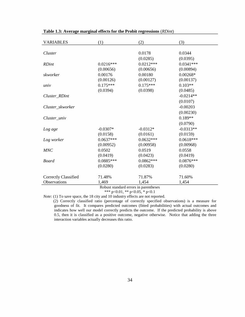
Three model specifications are estimated, the regression results being reported in Table

1.3: specification (1) is the baseline model; specification (2) includes the location

variable Cluster to establish whether being located in a cluster has any discernible effect

on new product introduction; and specification (3) also includes three interaction terms

for the variable Cluster and the three innovation input variables (Cluster_RDint,

Cluster_skworker, Cluster_univ) in order to establish whether being in a cluster changes

the effect innovation inputs have on innovation performance.

In a nonlinear model such as Probit, interpretation of the coefficients is not

straightforward instead marginal effects are more informative than coefficients.

21

Commonly used are marginal effects at means or at a representative set of values, as well

as average marginal effects. In this analysis average marginal effects are reported. For

purposes of interpretation, the baseline specification is used as an example. In this case,

if R&D intensity (RDint) had increased by 10 percentage points, then on average the

probability of innovation would have increased by about 21.6 percentage points. Having

a university link (univ) would on average have increased the likelihood of innovation by

17.5 percentage points. In other words, the predicted probability of introducing new

products would have been 17.5 percentage points higher for firms with a university link

than it would have been for firms without.

Of the three specifications, (1) and (2) generate very similar results in terms of

sign, magnitude, statistical significance and confidence intervals, suggesting that the

inclusion of the Cluster variable does not affect the baseline model results. This

similarity in results also extends to specification (3) for the four firm attribute control

variables. In other words, there are little changes to the coefficients of these four

variables in all three specifications. All the individual predictor variables have the

expected signs, among which the variables for RD intensity (RDint), university link

(univ), firm age (log age), firm size (log worker), and corporate governance (Board) are

statistically significant in all three specifications. One of the innovation input measures,

skilled worker (skworker), is only statistically significant in specification (3). The

foreign influence variable (MNC) shows no statistical significance in any of the

specifications. The main variable of interest Cluster is not found to be statistically

significant, either.

22

Of the three interaction terms, two of them are statistically significant.

Cluster_univ is positive and statistically significant, suggesting locating in a cluster and

having a university link boosts innovation. However, Cluster_RDint is negative and also

statistically significant, a result that would seem to suggest that being in a cluster reduced

the effectiveness of R&D on innovation. This result deserves more attention, which may

trace back to the quality of this variable.

In order to capture the extent of R&D effort, the ratio of R&D and sales provides

useful information. However, the R&D expenditure variable has excessive zeros. In

fact, 60 percent of the observations for this variable are zeros. It is hard to pin down

whether these are true values or measurement errors. Perhaps it is not surprising,

considering that the R&D spending variable in innovation surveys is often of low quality

or not even answered (Mairesse and Mohnen, 2010). In order to reduce variability in this

variable, a dummy variable called RD is created to replace the RDint variable. If a firm

incurred R&D expenditure in the previous two years (2000-2001), then RD is coded as 1,

and 0 otherwise. As a result, the firms are divided into two groups: R&D performers and

nonperformers. The regression results with the new RD variable are reported in Table

1.4.

Compared to the previous results reported in Table 1.3 (with R&D intensity), the

general pattern is very similar, except firm age (log age) and university link (univ) are no

longer statistically significant across all three specifications, in addition, the magnitude of

the consistently significant variables also see a reduction in magnitude. The major

differences are in specification (3): the variable for university link (univ) loses its

23

statistical significance and its magnitude drops quite a bit. Adding the interaction terms

seems to have a big effect on this variable, suggesting that many of the firms that had

university links were located in clusters. The interaction term Cluster_RD has a negative

coefficient but statistically insignificant. Like R&D intensity, the R&D dummy is

positive and consistently significant. Now if a firm conducted R&D (regardless of the

level), on average the probability of innovation is estimated to have increase by 20

percentage points (baseline specification result). But all in all, the Cluster variable is still

statistically insignificant when R&D intensity is replaced by R&D dummy.

ii. Subsamples

The results reported so far suggest that clustering does not have a discernible effect on

firm innovation. Next, to check if there will be any changes to statistical significance or

coefficient magnitude, the sample is broken down by region (coastal and inland) and by

industry (high-innovation and low-innovation rates).

Coast vs. inland

There exists a prominent coast-inland divide in China. It mainly refers to the gap in

economic development between these two regions (Démurger et al., 2002). Due to its

geographic advantage, the coastal area has received preferential treatment since the

beginning of the reform era in the late-1970s, the early clusters being concentrated in the

coastal region. Generally speaking, clusters in coastal areas are more mature, and

consequently, their effect on innovation may be different from that inland. Out of the 18

cities covered in the survey, 5 are on the coast: Wenzhou, Shenzhen, Jiangmen, Dalian,

and Hangzhou. These 5 cities account for 333 firms in the sample.

24

High-innovation vs. low-innovation industries

The sample is also grouped according to innovation rates: above average and below

average. The mean innovation rate is approximately 0.444 for the entire sample. The

four industries that have above average innovation rates are: electronic equipment,

electronic parts making, household electronics, auto & auto parts (see Table 1.1). These

four industries account for 882 firms in the sample.

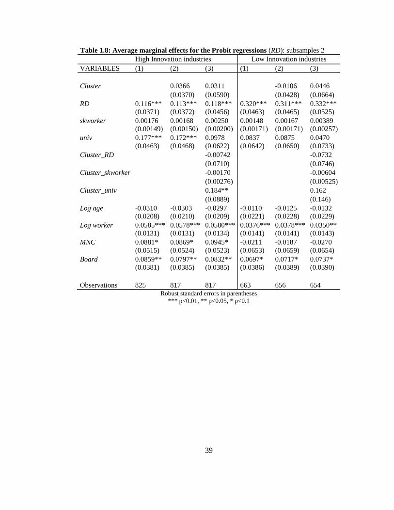
Regressions are then performed according to the above groupings of the sample,

with the results being reported in Tables 1.5-1.8, based on the split between either the

R&D intensity or the R&D dummy. Three variables are consistently positive and

statistically significant across subsamples and specifications: the R&D measures (both

R&D intensity and R&D dummy), firm size (log worker), and corporate governance

(Board). The Cluster variable remains statistically insignificant. It is worth noting that

the positive effect of Board on innovation was much stronger for firms in coastal cities

than for those in inland cities. This result seems to suggest that corporate governance is

more effective in firms on the coast. The coefficients for university link are only positive

and statistically significant for inland firms, indicating universities have a larger role in

helping inland firms developing new products. Also worth noting is that the impact of

R&D on new product introduction was larger for firms belonging to the low innovation

industries than those in high innovation industries. MNCs also had an edge in high

innovation industries even though the statistical significance is weak.

Cluster, the main variable of interest, is found to have no statistical significance,

either in the full sample or in the subsamples. This finding is in line with the group of

25

studies (discussed in section 3) that have found that, after controlling for firm-specific

factors, being located in a cluster per se does not have any discernibly positive effect on

firm innovation.

7. Alternative Hypothesis

On the one hand, we do observe in our sample that firms in clusters were more

innovative. The data clearly indicate that the innovation rate was much higher for firms

inside clusters than those outside clusters (64% vs. 42%). But on the other hand it has

also been established from the econometric analysis thus far that cluster location by itself

has no statistically significant effect on a firm’s propensity to innovate. So what is it

about clusters that result in firms possessing qualities that make them more innovative?

We will examine the predictor variables once again, this time focusing on the differences

between clustered and non-clustered firms. The summary statistics are presented in

Table 1.9.

Comparison between the two groups reveal that clustering firms were associated

with higher R&D intensity, a larger skilled worker ratio, they were younger and larger

firms that were more likely to have a university link, foreign ownership and corporate

board - all the features possessed by innovative firms in our sample. Is it coincidence?

What makes such firms locate in clusters? Alternatively, what makes firms in clusters

acquire such features? In other words, do clusters attract more innovative firms or

generate more innovations?

26

In a free market, private companies choose to congregate in order to take

advantage of “localization economies”. In China’s transitional economy, location

choices are still constrained and highly influenced by government directives. Firms are

often selected or admitted to be located in a cluster with various preferential supports by

government agencies. Based on interviews and survey responses, Walcott (2003) found

that location choices of MNCs within China for manufacturers were constrained by two

factors: government directives specifying the particular location(s) within a city; the other

major factor is the need to be close to a joint venture partner’s location. For Chinese

companies in industrial or science parks, the issue of affiliation ties to a region or

university is the deciding factor.

Given that firms generally do not self-select to be in a cluster, selection by the

government cannot be ruled out and could be a concern, however it cannot be observed.

Next we ask if and how cluster location shapes a firm’s innovative activity.

The most often reported explanation of innovation output is R&D effort

especially the fact of performing R&D on a continuous basis. This variable has a

statistically significant and positive effect on innovation in almost all studies (Mairesse

and Mohnen, 2010). This is also confirmed by our results. Of the three innovation input

variables used in our model, R&D (whether intensity or dummy) is consistently positive

and statistically significant across specifications and samples. Lee (2009) investigated

the causal effect between cluster and R&D intensity his results showing that being

located in a cluster per se actually has a negative effect on firm R&D intensity. Bagella

27

and Becchetti (2002) found that geographic proximity has a negative impact on both

firm’s RD expenditures and decision to invest in RD.

The above mentioned studies both seem to suggest a negative cluster-RD

relationship. However, their results are all based on analysis of market-induced clusters.8

As introduced earlier, Chinese economic zones are built and run on a different model that

involves strong government participation. Next, an alternative hypothesis is proposed:

clustering matters for innovation result through an indirect effect, that is, by influencing

innovation inputs (specifically R&D).

To test the cluster-R&D relationship, two more factors will be considered:

1) R&D financing: empirically there is a strong relationship between access to

finance and innovation. For internal finance, a commonly used indicator in the literature

is cash flows, a measure of liquidity. As a possible determinant of R&D, cash flow may

be the most thoroughly examined firm characteristics in the literature (Cohen, 2010).9

However, this exact measure is not collected by the ICS survey. Instead, the ratio of

profit to capital, a measure of profitability, is used to indicate a firm’s internal finance.

With regard to external finance, in their investigation of the determinants of firm

innovation in over 19,000 firms across 47 developing economies based on a cross-

country ICS, Ayyagari et al. (2007) find that access to external financing is associated

with greater firm innovation, with bank financing being the most dominant form relative

to financing from all other sources. Based on available data, a dummy variable Credit is

8 Lee (2009) tested a subsample that only included firms in China and India and found a statistically

insignificant cluster-R&D relationship. 9 In addition, size (and age) is correlated with a firm’s financial position. Compared with small and young

firms, large and established firms appear to prefer internal funds for financing R&D investments and they

manage their cash flow to ensure this (Hall and Lerner, 2010).

28

created to indicate whether a firm has an overdraft facility or line of credit. It is not hard

to imagine that a firm that has credit constraints will be less willing to invest in R&D and

have trouble making such investments.

2) Appropriability condition: the conditions governing an innovator’s ability to

capture the returns from innovation, that is, appropriability, are found to be a determinant

of innovation (Cohen, 2010). It is widely believed that under weak appropriability

regimes, firms will be less willing to invest in R&D because other firms can just free ride

on them. A question in the ICS survey asks “what’s the likelihood that the legal system

will uphold your contract and property rights in business disputes?”. Even though the

words “intellectual property rights” were not specifically mentioned in the question, this

variable is loosely used as a proxy for appropriability condition. The industry dummies

are supposed to pick up the general appropriability condition in each industry, however,

this self-perceived survey question answer directly reflects individual firms’ willingness

to invest in property (including intellectual property).

The regression results based on this analysis are presented in Table 1.10. The

dependent variable is RD (the dummy) or RD intensity, both 2002 values. RDint is left-

censored as a significant portion of the observed values are zero and the rest positive

values. Correspondingly, a Probit model and a Tobit model are estimated respectively,

each with two specifications – one includes the Cluster variable and the other does not.

Values of the predictor variables are lagged whenever possible. Of the three additional

variables, Profitability (internal finance) shows no statistical significance, but the dummy

variable Credit (access to external finance) turns out to be positive and statistically

29

significant, and the variable Property Rights has no statistically significant impact on

R&D. log age (negative effect), log worker (positive effect) and Board (positive effect)

are all statistically significant. The Cluster variable is positive and statistically

significant in both models.

The overall results suggest clustering by itself is not conducive to better

innovation performance. It is through its positive influence on important innovation

input such as R&D expenditure that firm clustering makes a difference in innovation

performance. In our sample, the Cluster variable does not seem to have the spillover

effect predicted by the geography of innovation theories, instead it positively affects

R&D input contrary to previous studies’ findings (of the negative cluster-R&D link). It

is suspected therefore that the nature of these clusters, namely, the strong and proactive

involvement by the governments at all levels, makes the difference. Firms in these

development zones are often mandated to make a certain amount of R&D investment to

be qualified to locate in these zones. In other cases, they receive government subsidies

for R&D investment. For instance, since 2000 the Tianjin Economic Development Area

(TEDA), China’s top industrial park, has officially made technology investment a

priority. Subsidies amounting to five percent of the zone’s revenues have been reinvested

in technology infrastructure. In the meantime, TEDA has offered grants worth millions

of RMB to incubate a wide range of companies, including startups, growing companies

and well established companies.

30

8. Summary and Conclusions

Since the early days of the economic reform, Chinese governments at different levels

have been building development zones of various kinds in order to accelerate growth in

designated locales and industries. This essay examines the impact of this spatial setup on

firm innovation based on theories in the geography of innovation and data from a 2003

Chinese firm survey. Initial analysis indicates that clustered firms are associated with a

higher rate of new product introduction. To test the first hypothesis of whether firm

clustering leads to higher propensity of innovation, a Probit model has been estimated.

When the effect of cluster is isolated, i.e., after innovation inputs, firm attributes, city and

industry effects are controlled for, the Cluster variable fails to show statistical

significance, in spite of different model specifications and sample groupings. Next,

following Lee (2009), a second hypothesis is tested to establish if clustering induces

better innovation performance by way of influencing R&D effort. The results indicate

that clustering does have a positive effect on both firm’s decision to invest in R&D and

R&D intensity.

The approach in this essay is different from many cluster studies in the sense that

it does not focus on any specific clusters, what was done instead was to assess the general

effect of locating in a cluster-like environment across China. While such an approach

inevitably produces rather generalized results, it does allow capture of an overall picture

of clustering effect on Chinese firm innovation.

Wang (2007) has emphasized that geographical proximity alone will not generate

agglomeration economies (proximity does not equal agglomeration). There should also

31

be close industrial linkages in order for the firms to enjoy external economies of scale.

Based on her field studies, she advised that governments should not just focus on creating

geographic proximity, but also on promoting industrial linkages among clustering firms.

Clustering can be a basis for stimulating the local innovation environment, but putting

firms in development zones to create “compelled proximity” often creates more problems

than what it solves. It is not surprising that in 2004 the central government started

curbing and shutting down development zones that were results of blind expansion. By

the end of 2006, the number of development zones/industrial parks had been reduced to

1,568 from nearly 7,000 at peak (Zeng, 2011).

In the analysis presented here, it is also revealed that the corporate governance

variable (Board) has a particularly strong effect on new product introduction for firms on

the coast, suggesting that a board of directors is not as widely implemented or not as

effectively implemented in inland firms. Also the impact of conducting R&D on new

product introduction is much stronger for firms in low-innovation industries than those in

high-innovation industries. Governments should strengthen incentives to encourage

firms in lagging industries to carry out more innovation activities.

All resources needed to generate innovation are hardly confined to individual

firms, thus a larger context should be considered. This essay adds a geographic context

to Chinese firm innovation studies. Our conclusion is that clustering does not necessarily

contribute directly to the innovative activities of firms, but it does influence firms R&D

input positively. Future direction will be focused on finding out specific channels

through which clustering affects R&D effort.

32

9. Figures and Tables

Figure 1. 18 Chinese cities in the sample

33

Table 1.1: Distribution and innovation rates of firms in different industries

Industry Number of

Firms

Percent

(%)

Innovation

rate

Garment & leather products 353 21.84 .2722063

Electronic equipment 185 11.45 .6

Electronic parts making 276 17.08 .5404412

Household electronics 63 3.90 .5806452

Auto & auto parts 358 22.15 .5354108

Food processing 71 4.39 .4153846

Chemical products & medicine 66 4.08 .3692308

Biotech products & Chinese

medicine

36 2.23 .4411765

Metallurgical products 158 9.78 .3227848

Transportation equipment 50 3.09 .244898

Total 1,586 100.00 .4440955 Source: Chinese Investment Climate Survey, 2003

Table1.2: Summary statistics

Variables Entire Sample Innovative firms Non-innovative firms

Mean Std. dev. Mean Std. dev. Mean Std. dev.

Cluster .2844444 .4512927 .3685714 .4827623 .2171429 .4125365

R&D intensity .0121522 .0485883 .0214119 .0689399 .0046698 .0174919

Skilled worker .1307023 .6908588 .1926834 1.018764 .0808512 .146702

University .1309599 .3374638 .2171429 .4125955 .0618557 .2410313

Age 15.48492 13.97523 14.85573 13.8311 15.98757 14.07691

Size 463.2215 1117.854 674.6176 1419.32 294.2005 758.4637

MNC .0998093 .2998409 .1432665 .3505956 .0651429 .2469189

Board .5282663 .4993572 .6633663 .472893 .420339 .4938924 Note: Number of observations varies depending on the variables.

34

Table 1.3: Average marginal effects for the Probit regressions (RDint)

VARIABLES (1) (2) (3)

Cluster 0.0178 0.0344

(0.0285) (0.0395)

RDint 0.0216*** 0.0212*** 0.0341*** (0.00656) (0.00656) (0.00894)

skworker 0.00176 0.00180 0.00268* (0.00126) (0.00127) (0.00137)

univ 0.175*** 0.175*** 0.103** (0.0394) (0.0398) (0.0485)

Cluster_RDint -0.0214**

(0.0107)

Cluster_skworker -0.00203

(0.00230)

Cluster_univ 0.189**

(0.0790)

Log age -0.0307* -0.0312* -0.0313** (0.0158) (0.0161) (0.0159)

Log worker 0.0637*** 0.0632*** 0.0618*** (0.00952) (0.00958) (0.00968)

MNC 0.0502 0.0519 0.0558 (0.0419) (0.0423) (0.0419)

Board 0.0885*** 0.0862*** 0.0876*** (0.0280) (0.0283) (0.0280)

Correctly Classified 71.48% 71.87% 71.60% Observations 1,469 1,454 1,454

Robust standard errors in parentheses

*** p<0.01, ** p<0.05, * p<0.1

Note: (1) To save space, the 18 city and 10 industry effects are not reported.

(2) Correctly classified ratio (percentage of correctly specified observations) is a measure for

goodness of fit. It compares predicted outcomes (fitted probabilities) with actual outcomes and

indicates how well our model correctly predicts the outcome. If the predicted probability is above

0.5, then it is classified as a positive outcome, negative otherwise. Notice that adding the three

interaction variables actually decreases this ratio.

35

Table 1.4: Average marginal effects for the Probit regressions (RD)

VARIABLES (1) (2) (3)

Cluster 0.0228 0.0343

(0.0282) (0.0425)

RD 0.196*** 0.192*** 0.206*** (0.0292) (0.0294) (0.0351)

skworker 0.00150 0.00154 0.00241 (0.00115) (0.00116) (0.00157)

univ 0.136*** 0.134*** 0.0681 (0.0384) (0.0388) (0.0482)

Cluster_RD -0.0414

(0.0524)

Cluster_skworker -0.00165

(0.00226)

Cluster_univ 0.179**

(0.0768)

Log age -0.0256* -0.0256 -0.0258 (0.0155) (0.0158) (0.0157)

Log worker 0.0491*** 0.0490*** 0.0482*** (0.00973) (0.00979) (0.00990)

MNC 0.0571 0.0570 0.0606 (0.0412) (0.0417) (0.0417)

Board 0.0791*** 0.0767*** 0.0786*** (0.0276) (0.0279) (0.0279)

Correctly Classified 71.51% 71.42% 71.24% Observations 1,488 1,473 1,471

Robust standard errors in parentheses

*** p<0.01, ** p<0.05, * p<0.1

36

Table 1.5: Average marginal effects for the Probit regressions (RDint): subsamples 1

Coast Inland

VARIABLES (1) (2) (3) (1) (2) (3)

Cluster -0.0475 -0.0768 0.0459 0.0750

(0.0570) (0.0760) (0.0334) (0.0471)

RDint 0.0300** 0.0297** 0.0235* 0.0204*** 0.0193*** 0.0417*** (0.0121) (0.0121) (0.0128) (0.00759) (0.00744) (0.0106)

skworker 0.00209 0.00237 0.00323 0.00176 0.00174 0.00271* (0.00258) (0.00260) (0.00378) (0.00142) (0.00144) (0.00145)

univ 0.131* 0.125 0.0383 0.191*** 0.194*** 0.119** (0.0787) (0.0826) (0.111) (0.0454) (0.0452) (0.0542)

Cluster_RDint 0.0464 -0.0319***

(0.0393) (0.0118)

Cluster_skworker -0.00240 -0.00254

(0.00480) (0.00271)

Cluster_univ 0.171 0.206**

(0.151) (0.0925)

Log age -0.0276 -0.0314 -0.0274 -0.0317* -0.0302* -0.0308* (0.0419) (0.0422) (0.0423) (0.0169) (0.0173) (0.0171)

Log worker 0.0693*** 0.0694*** 0.0721*** 0.0616*** 0.0611*** 0.0577*** (0.0223) (0.0227) (0.0227) (0.0106) (0.0106) (0.0106)

MNC -0.0470 -0.0278 -0.0239 0.0911* 0.0938* 0.0952* (0.0749) (0.0774) (0.0774) (0.0536) (0.0540) (0.0536)

Board 0.181*** 0.182*** 0.182*** 0.0695** 0.0648** 0.0635** (0.0653) (0.0659) (0.0648) (0.0313) (0.0316) (0.0311)

Observations 299 295 295 1,170 1,159 1,159

Robust standard errors in parentheses

*** p<0.01, ** p<0.05, * p<0.1

37

Table 1.6: Average marginal effects for the Probit regressions (RD): subsamples 1

Coast Inland

VARIABLES (1) (2) (3) (1) (2) (3)

Cluster -0.0446 -0.0741 0.0492 0.0736

(0.0567) (0.0861) (0.0331) (0.0497)

RD 0.221*** 0.223*** 0.217*** 0.192*** 0.182*** 0.201*** (0.0580) (0.0584) (0.0730) (0.0339) (0.0341) (0.0401)

skworker 0.00136 0.00162 0.00147 0.00169 0.00166 0.00281 (0.00247) (0.00248) (0.00374) (0.00129) (0.00131) (0.00171)

univ 0.0758 0.0626 -0.0309 0.155*** 0.157*** 0.0918* (0.0806) (0.0845) (0.110) (0.0439) (0.0438) (0.0536)

Cluster_RD 0.0217 -0.0550

(0.111) (0.0590)

Cluster_skworker -0.000250 -0.00227

(0.00444) (0.00265)

Cluster_univ 0.183 0.187**

(0.147) (0.0890)

Log age -0.0186 -0.0235 -0.0200 -0.0276* -0.0256 -0.0262 (0.0427) (0.0429) (0.0429) (0.0166) (0.0169) (0.0169)

Log worker 0.0527** 0.0529** 0.0544** 0.0470*** 0.0474*** 0.0461*** (0.0225) (0.0229) (0.0231) (0.0109) (0.0110) (0.0111)

MNC -0.00320 0.0137 0.0187 0.0805 0.0832 0.0876* (0.0738) (0.0768) (0.0768) (0.0526) (0.0534) (0.0530)

Board 0.179*** 0.179*** 0.182*** 0.0602** 0.0559* 0.0573* (0.0656) (0.0661) (0.0653) (0.0307) (0.0310) (0.0310)

Observations 300 296 296 1,188 1,177 1,175

Robust standard errors in parentheses

*** p<0.01, ** p<0.05, * p<0.1

38

Table 1.7: Average marginal effects for the Probit regressions (RDint): subsamples 2

High Innovation industries Low Innovation industries

VARIABLES (1) (2) (3) (1) (2) (3)

Cluster 0.0338 0.0430 -0.0236 0.0117

(0.0375) (0.0544) (0.0426) (0.0613)

RDint 0.0124* 0.0118* 0.0154 0.0446*** 0.0448*** 0.0793*** (0.00666) (0.00666) (0.0106) (0.0126) (0.0124) (0.0179)

skworker 0.00152 0.00144 0.00278 0.00331* 0.00351** 0.00365** (0.00155) (0.00156) (0.00201) (0.00171) (0.00171) (0.00170)

University link 0.200*** 0.196*** 0.125** 0.144** 0.149** 0.0783 (0.0465) (0.0469) (0.0613) (0.0688) (0.0697) (0.0773)

Cluster_RDint -0.00459 -0.0655***

(0.0133) (0.0210)

Cluster_skworker -0.00260 -0.00249

(0.00287) (0.00573)

Cluster_univ 0.179* 0.221

(0.0915) (0.153)

Log age -0.0330 -0.0323 -0.0314 -0.0221 -0.0256 -0.0282 (0.0208) (0.0211) (0.0209) (0.0232) (0.0238) (0.0237)

Log worker 0.0679*** 0.0670*** 0.0665*** 0.0576*** 0.0574*** 0.0551*** (0.0125) (0.0126) (0.0129) (0.0142) (0.0142) (0.0141)

MNC 0.0901* 0.0906* 0.0979* -0.0493 -0.0454 -0.0611 (0.0523) (0.0531) (0.0528) (0.0638) (0.0643) (0.0635)

Board 0.0953** 0.0893** 0.0924** 0.0732* 0.0754* 0.0781** (0.0383) (0.0387) (0.0384) (0.0394) (0.0396) (0.0391)

Observations 818 810 810 651 644 644

Robust standard errors in parentheses

*** p<0.01, ** p<0.05, * p<0.1

39

Table 1.8: Average marginal effects for the Probit regressions (RD): subsamples 2

High Innovation industries Low Innovation industries

VARIABLES (1) (2) (3) (1) (2) (3)

Cluster 0.0366 0.0311 -0.0106 0.0446

(0.0370) (0.0590) (0.0428) (0.0664)

RD 0.116*** 0.113*** 0.118*** 0.320*** 0.311*** 0.332*** (0.0371) (0.0372) (0.0456) (0.0463) (0.0465) (0.0525)

skworker 0.00176 0.00168 0.00250 0.00148 0.00167 0.00389 (0.00149) (0.00150) (0.00200) (0.00171) (0.00171) (0.00257)

univ 0.177*** 0.172*** 0.0978 0.0837 0.0875 0.0470 (0.0463) (0.0468) (0.0622) (0.0642) (0.0650) (0.0733)

Cluster_RD -0.00742 -0.0732

(0.0710) (0.0746)

Cluster_skworker -0.00170 -0.00604

(0.00276) (0.00525)

Cluster_univ 0.184** 0.162

(0.0889) (0.146)

Log age -0.0310 -0.0303 -0.0297 -0.0110 -0.0125 -0.0132 (0.0208) (0.0210) (0.0209) (0.0221) (0.0228) (0.0229)

Log worker 0.0585*** 0.0578*** 0.0580*** 0.0376*** 0.0378*** 0.0350** (0.0131) (0.0131) (0.0134) (0.0141) (0.0141) (0.0143)

MNC 0.0881* 0.0869* 0.0945* -0.0211 -0.0187 -0.0270 (0.0515) (0.0524) (0.0523) (0.0653) (0.0659) (0.0654)

Board 0.0859** 0.0797** 0.0832** 0.0697* 0.0717* 0.0737* (0.0381) (0.0385) (0.0385) (0.0386) (0.0389) (0.0390)

Observations 825 817 817 663 656 654

Robust standard errors in parentheses

*** p<0.01, ** p<0.05, * p<0.1

40

Table1.9: Summary statistics

Variables Entire Sample Innovative firms Non-innovative firms

Mean Std. dev. Mean Std. dev. Mean Std. dev.

RD .4182754 .4934347 .5717489 .495381 .3564982 .479181

RD intensity .0155229 .2545317 .0298944 .0784505 .0097352 .2971977

Profitability .0921647 .1058521 .1275551 .1359623 .0782155 .0875201

Credit .1373418 .3443168 .2008929 .401116 .1121908 .3157406

Property 63.27802 38.95964 68.86226 36.85075 58.62819 40.06632

Age 15.47055 13.94282 10.01762 9.394219 17.63835 14.83853

Size 463.5841 1117.007 550.3722 1321.649 429.0211 1022.8

MNC .0989848 .2987364 .196868 .3980773 .0602303 .2380185

Board .5269424 .4994301 .7555066 .4302605 .4360771 .4961143 Note: Number of observations varies depending on the variables.

Table 1.10: Regression results (cluster-R&D)

Probit Tobit

VARIABLES (1)

RD (2) RD

(3) RDint

(4) RDint

Cluster 0.0587* 2.620***

(0.0303) (0.711)

Profitability 0.00173 0.00233 0.0921 0.0985 (0.00618) (0.00621) (0.178) (0.173)

Credit 0.106*** 0.106*** 1.530** 1.425** (0.0292) (0.0294) (0.668) (0.660)

Property Rights 0.000535 0.000423 0.0128 0.00919 (0.000327) (0.000332) (0.00893) (0.00890)

Log age -0.0666*** -0.0625*** -1.231*** -0.973** (0.0160) (0.0163) (0.411) (0.394)

Log worker 0.0912*** 0.0908*** 1.072*** 1.081*** (0.00973) (0.00967) (0.281) (0.279)

MNC -0.0470 -0.0558 0.319 -0.00607 (0.0415) (0.0416) (1.189) (1.185)

Board 0.146*** 0.141*** 3.170*** 2.891*** (0.0290) (0.0292) (0.754) (0.731)

Observations 1,274 1,260 1,264 1,251

Robust standard errors in parentheses

*** p<0.01, ** p<0.05, * p<0.1

41

Essay 2: The Role of Intellectual Property Rights in Seed Technology Transfer through

Trade – Evidence from U.S. Field Crop Seed Exports

1. Introduction

Rising food prices driven up by food shortages in recent years have triggered social and

political unrest in some parts of the world (FAO, 2012). The importance of food security

is therefore, being brought back into the public policy spotlight. With a growing world

population but limited land and water resources, the world is increasingly reliant on

agricultural technology to raise food production. Seed is the basis of crop-based

agriculture. Together with other contributing factors such as fertilizers, pesticides,

herbicides and irrigation, improved seed varieties have been responsible for much of the

observed increases in global yields (UPOV, 2009).10

From conventional to hybrid to

genetically modified (GM) seeds, the plant breeding and seed industry has been

contributing to agricultural innovation.

The time-consuming nature and high costs associated with plant breeding puts

small companies in a disadvantaged position to take on formal research and development

(R&D) efforts. According to the International Seed Federation’s statistics, plant breeding

companies typically reinvest 12-15% of their sales in R&D with the top 20 companies

spending $4 billion every year on R&D. Moreover, the development cycle for a new

10

UPOV is the acronym for Union internationale pour la protection des obtentions végétales, the French

name of the International Union for the Protection of New Varieties of Plants.

42

variety usually takes 10-15 years. As a result, seed technologies are concentrated in a

relatively small number of large firms, most of them based in the U.S. or Europe. The

Big Six firms identified in a global seed industry study by Howard (2009) are split

equally between the U.S. and Europe. The self-replicating nature of (non-hybrid) seeds

makes plant breeding innovations embodied in seeds particularly susceptible to being

imitated or reproduced with minimal difficulty or at a low cost. Non-existent or

insufficient intellectual property (IP) protection will jeopardize breeders’ interests and

reduce private incentives for further innovation efforts. To recover costs and receive

proper returns on its R&D investment, the seed industry lobbies hard for stronger legal

protection of its innovations. With the advent of GM crops, the relevance and

significance of intellectual property rights (IPRs) have been intensified as more

proprietary seed technologies are involved. Over the years, IPRs such as patents and

plant breeder’s rights (PBRs) have been established to regulate the seed market and

confer exclusive rights, i.e., market power, for a limited period of time, thus giving the

incentive and means to finance R&D activities.

The form of intellectual property created by the conventions of the International

Union for the Protection of New Varieties of Plants (UPOV) is known as PBRs. As a

special purpose system, PBR laws only apply to plants and plant materials, whereas

under patent acts, almost everything is patentable. In addition to differences in protection

requirements, under PBR systems farmers are allowed to save seeds for future planting.

But under patents, seed saving would constitute infringement. Additionally, research

under PBR is a more clear-cut process than for patented inventions. Due to provisions

43

for farmer’s privilege and breeders’ rights, protection provided under PBRs is generally

considered to be weaker than under patents. This helps explain why commercial breeders

often prefer patents, or patents plus PBR, over PBR alone (Lesser, 2007).

Trade is an important channel through which technology gets transferred across

borders (Grossman and Helpman, 1995).11

Decisions by firms to export to a particular

market are influenced by the effectiveness of local IPRs. However, national laws vary.

To harmonize IPRs for cross-border trade, the World Trade Organization (WTO)

agreement on Trade Related Aspects of Intellectual Property Rights (TRIPs) went into

effect on January 1, 1995. It makes protection of IPRs an integral part of the multilateral

trading system. TRIPs, has made a set of minimum IP standards a requirement for all its

159 members, and is to date the most comprehensive multilateral agreement on

intellectual property. Furthermore, Article 27.3(b) of TRIPs also extends IPRs to new

plant varieties by stipulating that member states must provide for the protection of seeds

and plant varieties either by patents, or an effective sui generis system, i.e., a system

created especially for this purpose, such as the plant breeder’s rights provided in the

conventions of UPOV, or by any combination of the two. As a consequence, a country

might provide UPOV-like protection without joining UPOV as a result of being a

signatory of TRIPs.

If a country does not have legislation that is compliant with international IPR

standards or is lax in its enforcement of IRPs, seed companies may not want to sell to

11

Additional cross-border technology transfer mechanisms include licensing and foreign direct investment

(FDI).

44

growers in that country in order to retain control over proprietary information.12

But if

IPRs become too stringent, especially by developing countries standards, they may in fact

restrict market access. In either case, IPRs can act as a barrier to trade.

Another source of potential trade distortion is the acceptance or approval status of

GM crops in different countries.13

GM crops have been grown commercially since 1996,

initially in 6 countries on 1.7 million hectares to 29 countries with 160 million hectares

under cultivation by 2011 (James, 2011). Biotechnology innovations embodied in seeds

lower input and production costs as well as enhance crop quality and yield. However, not

all countries have embraced GM crops due to concerns over potential harmful effects on

human health and the environment (Singh et al., 2006). For instance, an EU moratorium

on approval of GM crops (1999-2004) caused trade disputes with the U.S., Canada and

Argentina that also affected seed trade (WTO DISPUTE DS291). The approval status of

GM crops therefore affects a country’s import decision with respect to transgenic seeds.

In order to contribute to the understanding of whether IPRs encourage or impede

seed technology transfer through trade, the objective of this essay is to assess the impact

of a country’s intellectual property rights (IPRs) on its seed imports from the U.S., a

global leader in seed production and exporting, and also to evaluate, if and how growing

GM crops affects this relationship. For two reasons, the focus is on one type of seeds –

field crop seeds. First, growth in the U.S. seed market has been particularly rapid for

12

Monsanto stopped selling soybean seeds in Argentina in the early 2000s when it could not enforce its

property rights (Kesan and Gallo, 2007). 13

Another possible non-tariff barrier is sanitary and phyto-sanitary standards (Jayasinghe, Beghin and

Moschini., 2009)

45

major field crops (Fernandez-Cornejo, 2004). Secondly, the four major GM crops are all

field crops – soybeans, maize, cotton and canola (James, 2011).

In this essay both linear and nonlinear fixed effects estimators are used to fit a

gravity model with data covering 134 countries over the period 1985-2010. The

remainder of the essay is organized as follows: in section 2, a review of a selected

number of key previous studies on IPRs and trade is presented; in section 3, the model

framework and data are outlined while in section 4 the estimation results and appropriate

robustness checks are discussed; finally section 5 contains a summary of the essay and

concluding remarks.

2. IPRs and Trade

With regard to how differing levels of IP protection across national borders influence

trade flows, theoretical work does not provide an unambiguous answer (Grossman and

Helpman, 1990; Grossman and Lai, 2004). Theoretical studies focus on two main

counteracting effects of IPRs on market access: market expansion and market power.

The market expansion effect increases trade flows toward countries with stronger IPRs

because of increased demand and lower marginal exporting costs as a result of a reduced

threat of imitation. In contrast, trade flows may decrease through the market power

effect, as IPRs provide monopolistic control of innovations and the holder of the IPR may

exercises their monopoly power by raising prices and restricting export volumes. IPR’s

net effect on trade depends on the relative magnitude of these two effects. It is further

46

complicated by firms’ decisions to engage in licensing or FDI rather than exporting.

Therefore, it is essentially an empirical question.

The empirical literature so far has been focused on manufactured goods, and

studies in this area generally find IPRs to have a significantly positive impact on either

OECD or U.S. exports in patent-sensitive sectors. Maskus and Penubarti (1995) present

the first systematic evidence on whether differential patent laws influence international

trade. Their analysis relies on trade data for a single year, 1984. Their results indicate

that stronger patent protection has a positive effect on manufacturing imports into both

small and large developing economies. Their finding also supports the view that trade

reduction through the exercise of enhanced market power is more important in patent-

sensitive sectors than in patent-insensitive sectors.

Using export data for 1992, Smith (1999) assesses the sensitivity of U.S. exports

to national differences in patent rights. He finds that in countries that pose a strong

threat-of-imitation, weak patent rights are a barrier to US exports, whereas in countries

that pose a weak threat-of-imitation, increasing patent rights reinforces monopoly power

and lowers U.S. exports to these markets.

Ivus (2010) evaluates the link between patent rights in developing countries and

exports from the developed world over the period 1962-2000. She finds strengthening of

IPR protection in response to TRIPs raised the value of patent-sensitive exports to

developing countries.

A few researchers have studied the relationship between IPRs and seed trade in

recent years. Yang and Woo (2006) is the first systematic study of IPRs and seed trade,

47

followed by Eaton (2009) and Galushko (2012). The first two articles utilize aggregate

seed data and fail to detect a significant effect of their IPR variables on trade in seeds.

The third article uses crop-level seed data and obtained different results. Using data on

60 countries over 1990-2000, Yang and Woo (2006) show that imports of planting seeds

from the US are not discernibly affected by a country’s adherence to international IPR

agreements, implying that agricultural trade does not seem sensitive to strengthening of

IPRs. With data spanning 19 years (1989-2007), Eaton (2009) also finds no significant

effect from UPOV membership on seed imports from 10 EU countries and the U.S. in 70

importing countries and suggests future research to narrow it to a single exporting

country and a specific category of seeds. Galushko (2012) analyzes U.S. seed exports of

11 crops to 137 countries over 1995-2005. She grouped these 11 crops by breeding

techniques and estimated a Heckman (1979) selection model, and showed that the impact

of plant related IPRs varies across different groups of crops. Her result being

encouraging, her method has an obvious limitation, namely, she did not control for fixed

effects (either country or time). This essay builds on these three studies by utilizing a

larger dataset and focusing on a subcategory of agricultural seeds – field crop seeds that

include seeds particularly susceptible to IPR infringement.

3. Model Framework and Data

Pioneered by Tinbergen (1962), the gravity model has been an empirical success in

explaining bilateral trade flows by exploring the impact of economic size and trade

48

barriers between countries. The model can be derived from a range of trade theories.14

The modularity of gravity also allows for disaggregation by goods which facilitates

analysis of frictions that are likely to differ markedly by product characteristics

(Anderson, 2011). A typical gravity equation resembles the following form:

)

X denotes trade volume; is a constant; Y denotes economic size; T represents trade

resistance or frictions such as distance-related transport costs between countries i and j.

The popularity of the gravity equation also lies in its flexibility. It can be augmented to

include a wide range of variables to capture country attributes and various measures of

trade barriers and enhancers such as tariffs, currency unions and preferential trade

agreements. Since the focus of the essay is on unilateral trade from the U.S. perspective,

only the variables of the destination country are included in the analysis. Essentially, a

crude import demand function is being estimated.

The dataset comprises a panel covering 134 countries spanning 26 years (1985-

2010). The 134 countries consist of any existing sovereign state that imported field crop

seeds from the U.S. at least once during the sample period and contains no missing values

in all the regression variables. 1985 was chosen as the sample starting point based on the

fact that it was the year when the global seed trade began growing rapidly (International

Seed Federation statistics). A description of data sources is included in Table 2.1, while

summary statistics are provided in Table 2.2. The dependent variable is the value of

14

See Anderson (1979), Bergstrand (1985), Deardorff (1998), Evenett and Keller (2002), Anderson and

van Wincoop (2003), Feenstra (2004).

49

annual national field crop seed imports from the U.S (seedIMP).15

The explanatory

variables can be grouped into two categories: (1) country economic and market sizes (2)

potential trade distortions (including both trade enhancers and barriers). The traditional

gravity equation also includes geographic distance between trading nations, but since

only fixed effects models will be used for analysis, this time-invariant factor will not be

identified, hence distance is not included in the models. Fixed effects (FE) models are

chosen over random effects (RE) models on the basis that the RE’s strong assumption of

zero correlation between the unobserved individual effects and explanatory variables is

hard to justify for practical reasons.

In variable category (1) the relevant economic and market size variables are

represented by country GDP (logGDP) and crop production (logCropProd) respectively.

GDP measures a nation’s economic size, with higher national incomes implying more

means to purchase. It is therefore expected to have a positive effect on seed imports from

the U.S. Gravity equations usually also include the exporting country’s GDP, but since

in this case there is only one exporting country, its coefficient is absorbed into the time

fixed effects. Crop production refers to a country’s combined production quantity of

cereals, coarse grain, and oilseed crops. This variable measures the size of a country’s

crop production sector, giving a sense of demand for field crop seeds. Crop production is

also highly correlated with arable land and population, two factors commonly seen in

gravity models to indicate a country’s market size.

In variable category (2) a dummy variable for Free Trade Agreements (FTA) with

the U.S. is included. FTAs generally open up foreign markets to US exporters by

15

U.S. planting seed export data are not detailed at the GM and non-GM level.

50

reducing barriers such as tariffs. According to calculations by the Office of the U.S.

Trade Representative, for 16 of the 20 countries that the U.S. has FTAs in force with,

U.S. exporters will face zero tariffs on 98% or more of agricultural goods once the

agreements are fully implemented. The top two field crop seed importers during the

sample period are Mexico followed by Canada, both are parties to NAFTA.

Also included in variable category (2) are dummies for UPOV and TRIPs

membership as well as planting status of GM crops (growGM). The first UPOV

Convention went into force in 1968. Its two most recent revisions are referred to as the

“1978 Act” and “1991 Act”, of which almost all of its 70 member states are signatories

(not including the EU).16

The 1991 Act is more-strict in terms of coverage, period, scope

and exemptions. The U.S. has been a UPOV member since 1981 and upgraded to the

1991 Act in 1999. It is reasonable to assume that U.S. seed companies will have more

IPR concerns when they decide to export to a country that is not a UPOV member or only

conforms to the 1978 Act. Even though new members can no longer sign up to the 1978

Act, existing members who still stick with the 1978 Act are not obligated to upgrade. As

of 2010, among the 134 countries considered for this study, 64 are UPOV members, 22

adhere to the 1978 Act, and 41 are signatories of the 1991 Act (of which 14 countries

upgraded from 78 Act to the 91 Act).

To capture the effect of TRIPs, a transition period is considered. Supposedly

TRIPs applies once a country joins the WTO. However, different transition periods of

time to delay applying its provisions are allowed for members based on levels of

economic development. Specifically, developed countries among the original members

16

Belgium is the only country that is still on the 1968/1972 Act.

51

(countries that joined the WTO on January 1, 1995) were granted one year (until January

1, 1996) to ensure that their laws and practices conform with the TRIPs agreement.

Developing countries and (under certain conditions) transition economies were given a

further period of four years to apply the TRIPs Agreement’s provisions by January 1,

2000. 63 countries in our sample fall into this category. Least developed countries

(those recognized by the United Nations) were initially allowed until January 1, 2006 to

apply the provisions, now extended to July 1, 2013 with the possibility of further

extension, and until January 1, 2016 for pharmaceutical patents. 24 countries in the

sample belong to this group. Thus, two indicator variables are employed. WTO_TRIPs

refers to WTO member countries that have implemented the TRIPs agreement, while

WTO_trans represents WTO member countries that have been granted a TRIPs transition

period. Note that many of these members put into effect national legislation to

implement much of the TRIPs Agreement before the allowed transitional period expired,

but information on the exact timing is unavailable. Instead of trying to disentangle the

separate effects of TRIPs and WTO on trade, the difference between these two variables

(both contain the effect of WTO on trade) may provide guidance on the effect of TRIPs,

as some countries are using the TRIPs transition period while others are not.

Unlike membership of UPOV or TRIPs, GM crop planting status is not invariant

once started. In some European countries such as France, planting of GM crops was

discontinued during the early 2000s as France and five other EU countries banned GM

crops around the time that the EU moratorium on GM crop approval was in effect (James,

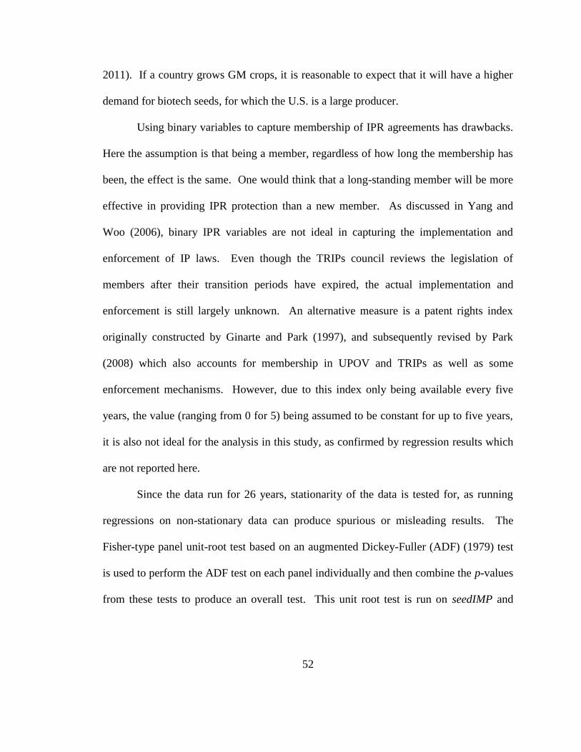
52

2011). If a country grows GM crops, it is reasonable to expect that it will have a higher

demand for biotech seeds, for which the U.S. is a large producer.

Using binary variables to capture membership of IPR agreements has drawbacks.

Here the assumption is that being a member, regardless of how long the membership has

been, the effect is the same. One would think that a long-standing member will be more

effective in providing IPR protection than a new member. As discussed in Yang and

Woo (2006), binary IPR variables are not ideal in capturing the implementation and

enforcement of IP laws. Even though the TRIPs council reviews the legislation of

members after their transition periods have expired, the actual implementation and

enforcement is still largely unknown. An alternative measure is a patent rights index

originally constructed by Ginarte and Park (1997), and subsequently revised by Park

(2008) which also accounts for membership in UPOV and TRIPs as well as some

enforcement mechanisms. However, due to this index only being available every five

years, the value (ranging from 0 for 5) being assumed to be constant for up to five years,

it is also not ideal for the analysis in this study, as confirmed by regression results which

are not reported here.

Since the data run for 26 years, stationarity of the data is tested for, as running

regressions on non-stationary data can produce spurious or misleading results. The

Fisher-type panel unit-root test based on an augmented Dickey-Fuller (ADF) (1979) test

is used to perform the ADF test on each panel individually and then combine the p-values

from these tests to produce an overall test. This unit root test is run on seedIMP and

53

logGDP. The null hypothesis is rejected in most cases, the conclusion being that not all

panels contain unit roots. The test results are presented in Tables 2.3 and 2.4.

4. Estimation

As explained earlier, the empirical analysis is based on the gravity model. To estimate

the gravity model of trade, the conventional approach is to first make the model linear by

taking logs and then estimate it through the ordinary least squares (OLS) method.

Although simple to implement, this approach becomes problematic when there are many

zero trade observations in the data because the log-linearized model is not defined for

observations with zero trade. 17

A common practice is to discard the zeros and run a

regression on the truncated and strictly positive data. Another approach is to add a small

positive value such as 1 to all the observations. If zeros either occur randomly or the

occurrence of zeros is small, then exclusion of these values should not significantly affect

the results. However, as Anderson (2011, p. 147) points out, “the prevalence of zeros

arises with disaggregation, so that in finely grained data, a large majority of bilateral

flows appear to be inactive.” Helpman, Melitz, and Rubinstein (2008) were confronted

with the problem of zeros (about half of the observations) in their analysis of country-

level trade flows. They admit the problem of zeros is even more severe at the industry

level. That is, in data sets of sectoral trade flows the fraction of zeros is much larger. If

the observations with zeros are dropped, that reduces the number of observations used in

actual estimation significantly and may lead to biased results. Consequently, an

17

Another problem is that the least squares estimator may be both biased and inefficient in the presence of

heteroskedasticity (Westerlund and Wilhelmsson, 2011).

54

estimation method is required that allows prediction of both zero and nonzero trade

values.

In this dataset, zeros constitute approximately 49 percent of the recorded import

observations. There is not a single missing value. A closer look reveals that zeros are

recorded for countries even before they came into existence. For instance, the Czech

Republic became an independent state in 1993 (after Czechoslovakia dissolved into two

constituent parts), so from 1985-1992 it should not have any observations, but in the

USDA export database they show up as zero trade flows. Of the 134 countries, 20 gained

independence after 1985. Such recording naturally leads to questioning of the validity of

all zero values. Some of these zeros might be true zeros, but others might represent

missing values. If the zeros are treated as missing values, then the gravity equation can

be log-linearized for estimation without rendering any observations invalid.

Alternatively, if the zeros are treated as true zeros, then they can be dealt with using

techniques such as Poisson regression model that predicts both zero and positive values.

Linear Fixed-Effects Model

This model is specified as:

)

where yit denotes field crop seed imports by country i during year t, αi is an unobserved

country fixed effect, is an error term, is a vector that contains the exogenous

explanatory variables.

More specifically, the following equation is estimated,

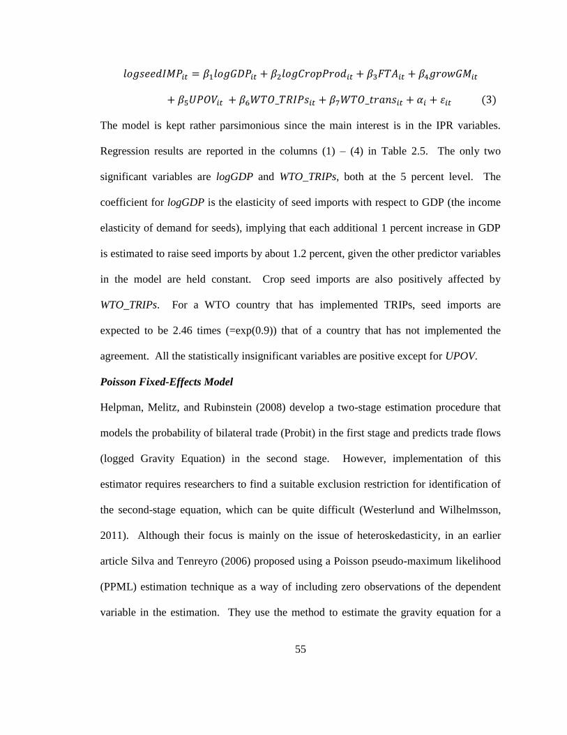
55

)

The model is kept rather parsimonious since the main interest is in the IPR variables.

Regression results are reported in the columns (1) – (4) in Table 2.5. The only two

significant variables are logGDP and WTO_TRIPs, both at the 5 percent level. The

coefficient for logGDP is the elasticity of seed imports with respect to GDP (the income

elasticity of demand for seeds), implying that each additional 1 percent increase in GDP

is estimated to raise seed imports by about 1.2 percent, given the other predictor variables

in the model are held constant. Crop seed imports are also positively affected by

WTO_TRIPs. For a WTO country that has implemented TRIPs, seed imports are

expected to be 2.46 times (=exp(0.9)) that of a country that has not implemented the

agreement. All the statistically insignificant variables are positive except for UPOV.

Poisson Fixed-Effects Model

Helpman, Melitz, and Rubinstein (2008) develop a two-stage estimation procedure that

models the probability of bilateral trade (Probit) in the first stage and predicts trade flows

(logged Gravity Equation) in the second stage. However, implementation of this

estimator requires researchers to find a suitable exclusion restriction for identification of

the second-stage equation, which can be quite difficult (Westerlund and Wilhelmsson,

2011). Although their focus is mainly on the issue of heteroskedasticity, in an earlier

article Silva and Tenreyro (2006) proposed using a Poisson pseudo-maximum likelihood

(PPML) estimation technique as a way of including zero observations of the dependent

variable in the estimation. They use the method to estimate the gravity equation for a

56

cross section of 136 countries in 1990. In comparison, they found biases present in both

the traditional specification of the gravity equation and in the Anderson-van Wincoop

(2003) specification (which includes country-specific fixed effects). Westerlund and

Wilhelmsson (2011) explore and extend upon an idea first pointed out by Wooldridge

(2002), namely that the fixed effects panel Poisson Maximum Likelihood (ML) estimator

can also be applied to continuous variables.18

They applied this technique with a panel

structure and suggest using the Poisson fixed effects estimator which performs well in

small samples in comparison to linear estimates. Their Poisson fixed effects approach is

also adopted in this study, the following equation being estimated in levels:

) )

The notation here is the same as in the linear model. More specifically, the following

equation is estimated:

) )

The fixed-effects Poisson regression results are reported in Table 2.5 columns (5) – (8).

As with the linear model, only logGDP and WTO_TRIPs are significant (at the 1 percent

and 5 percent levels respectively). While the number of countries stays the same, the

number of observations almost doubles. Using the results for specification (8) by way of

illustration, a 1 percent GDP increase leads to about a 2 percent increase in seed imports.

U.S. seed exports to a WTO member country that has implemented TRIPs is about 3.25

(=exp(1.18)) times that of a country that has not implemented TRIPs. All the statistically

18

It is also confirmed by Cameron and Trivedi (2010) that the Poisson FE estimator can be applied to any

model of multiplicative effects and an exponential conditional mean, essentially whenever the dependent

variable has a positive conditional mean.

57

insignificant variables are positive except for FTA. Compared to the linear model results,

the magnitude of the two significant variables are larger in the Poisson fixed effects

models – for logGDP it is 1.2 percent vs. 2 percent, and for WTO_TRIPs it is 2.46 times

vs. 3.25 times.

Robustness checks

The number of observations in the Poisson regression is almost twice that of the linear

regression. To make the results more comparable, the Poisson model is run again, this

time on the same observations used by the linear regression, i.e. the observations of

positive trade. The results are show in columns (5) – (8) of Table 2.6, the full-sample

results are included for comparison. The same result pattern is obtained except the

Poisson coefficients for the two significant variables have larger magnitudes than the

Poisson results on the full sample, which is expected.

Next a more detailed treatment of UPOV membership is considered. Eaton

(2009) differentiated between the 1978 Act and the 1991 Act. His coding of these two

variables is based on the assumption that if a country is a signatory of the 1991 Act, then

it also conforms to the 1978 Act since the 1991 Act is a stronger version of the 1978 Act.

But he does not account for the difference between a country that upgraded from the

1978 Act to the 1991 Act from a country that directly signed up to the 1991 Act. There

are four possible scenarios with regard to a country’s involvement in UPOV at different

points in time: 1) they are a signatory of the 1978 Act, but not the 1991 Act yet

(UPOV10); 2) they are a signatory of the 1991 Act, but previously did not sign up to the

1978 Act (UPOV01); 3) they are a signatory of the 1991 Act having upgraded from the

58

1978 Act (UPOV11); 4) they have no participation in either Act (the excluded group).

The idea is that there will be an additional effect for these countries who upgraded to the

1991 Act from the 1978 Act compared to those who signed up to the 1991 Act without

experiencing the 1978 Act. The models are refitted when UPOV is replaced with

UPOV10, UPOV01 and UPOV11 (the results being reported in Table 2.7). In the linear

models, the coefficient for UPOV01 is significantly negative, meaning this stringent act

probably reduces seed trade through the market power effect. But this result does not

carry over to the Poisson model. Other than that, logGDP and WTO_TRIPs are still the

only two statistically significant variables, maintaining the same signs and similar

magnitudes. The results from a comparable sample size are reported in Table 2.8.

The estimation method is then applied to a smaller set of countries: when

countries that have imported less than 10 times from the U.S. during the 26-year period

are discarded, with this filter 64 countries remain in the dataset. Because no country

traded 10 times, this serves as a natural gap. The numbers of observations are much

closer between the two models (1383 vs. 1582) once this criterion is applied. Even then,

a comparison shows the regression results, reported in Table 2.9, are very similar to those

of the full 134-country sample. This would seem to suggest that results of estimation of

the model do not depend on frequency of trading. The magnitudes of the two significant

variables are slightly larger. By reducing the sample size, there is potential for selection

bias to be introduced, as countries that import less may be excluded because they have

weak IPRs. Nonetheless, the hope is to reduce irregularity or idiosyncrasy by focusing

on countries on which there are more observations. Statistically speaking, the underlying

59

regression relationship can be better identified with data points of more regular

occurrences.

Linear Dynamic Panel Data Models

For countries that traded a lot in the past, exporters are likely to have set up distribution

and service networks in the partner country, resulting in entry and exit barriers due to

sunk costs. This argument can be traced back to the beachhead or sunk-cost effect

discussed in Baldwin’s article (1986) on hysteresis in import quantities. In addition,

consumers have grown accustomed to the partner country’s products (habit formation). It

is therefore very likely that trade patterns are highly persistent (Bun and Klaassen, 2002).

Olivero and Yotov (2012) have also argued that trade barriers imposed at time (t-1) might

still have an impact on trade volumes at time t. Consequently, it is important to evaluate

the effect of previous period(s) on subsequent period(s).

Statistically, in panel data y is observed over time, opening up the possibility that

y is dependent in part on its values in preceding periods. If in the true relationship the

dependent variable yi,t is partly dependent on the lagged dependent variable (yi,t-1 and so

on), then omitting yi,t-1 from the right hand side will cause the idiosyncratic errors to be

serially correlated (which will bias the standard errors). Wooldridge (2002) derives a

simple test for autocorrelation in panel-data models.19

Wooldridge’s test for within panel

serial correlation is run on the linear and nonlinear fixed effects models, and the null

hypothesis (of no autocorrelation) is strongly rejected. The most common solution is

adding a lagged dependent variable, that is, to run the dynamic model.

19

In this method, the first step is to run a regression of the pooled (OLS) model using first differences and

then predict the residuals. The second step is to run a regression of the residuals on their first lag and test

the coefficient on those lagged residuals.

60

Dynamic panel models include one or more lags of the dependent variable as

regressors. For a fixed effects (or random effects) model, consistent estimators can be

obtained by instrumental variable (IV) estimation in the first difference model, using

appropriate lags of regressors as the instruments (Cameron and Trivedi, 2009). Consider

an autoregressive model of order 1 (AR(1)) for yi,t (lgseedIMP) with 26 years of data

(1985-2010):

)

The notation here is the same as in the models previously introduced. Use first difference

to remove the fixed effect,

)

The first two years of data are lost in order to construct Δyi,t-1. Also, Δyi,t-1= yi,t-1 – yi,t-2 is

correlated with Δεi,t = ε i,t – εi,t-1 because yi,t-1 depends on εi,t-1.

Arellano and Bond (1991) developed a consistent generalized method of moments

(GMM) estimator that uses moment conditions in which lags of the dependent variable

and first differences of the exogenous variables are instruments for the first-differenced

equation. Specifically, Δyi,t-1 is instrumented using one or more subsequent lags, i.e., yi,t-2

and back, because they are uncorrelated with Δεi,t. Differences of the exogenous

variables serve as their own instruments.

The lagged levels can be rather poor instruments for first differenced variables,

especially if the variables are close to a random walk. A system estimator named after

Arellano and Bover (1995) and Blundell and Bond (1998) uses additional moment

conditions in which lagged first differences of the dependent variable are instruments for

61

the level equation. This estimator provides more precision, but the cost of the system

GMM estimator involves a set of additional restrictions on the initial conditions of the

process generating y.

Both estimators are built on a crucial assumption that the idiosyncratic errors are

serially uncorrelated otherwise the moment conditions of these GMM estimators will be

invalid. This assumption is testable by the Arellano-Bond test. This autocorrelation test

is a test of whether Δεi,t is correlated with Δεi,t-k for k ≥ 2, based on the correlation of the

fitted residuals. If εi,t are serially uncorrelated, it is expected to be rejected at order 1 but

not at higher orders because at order 1 the first differences are necessarily autocorrelated.

These two estimators are applied to the first differenced AR (1) model (6). The

regression results are reported in Tables 2.10 to 2.13. All regressions include the first lag

of y (yi,t-1) as a regressor. Unless otherwise noted, only the first available subsequently

lagged y are used as an instrument (so that just yi,t-2 is the instrument in period t).

The baseline results using the Arellano-Bond estimator are presented in Table

2.10. Columns (1) – (4) are based on the full sample covering 86 countries. Only two

variables, the lagged L.lgseedIMP and logCropProd, are consistently significant (both at

the 1 percent level). Their positive coefficients indicate that the more a country imports

seeds from the U.S. in previous year, the more it will import during the current year; the

higher the crop production capacity, the more the seed import. Columns (5) – (8) are

based on the reduced sample of countries that have imported seeds from the U.S. more

than 18 times during the 26-year sample period. The number of countries drops to 48

(from 86), but the number of observations decreases only by about 200. L.lgseedIMP and

62

logCropProd remain consistently significant and positive, with larger magnitudes. In

addition, the two WTO variables have gained in statistical significance (also at the 1

percent level). The coefficient of WTO_TRIPs is slightly higher than that of WTO_trans,

suggesting that WTO member countries that have implemented TRIPS have an advantage

in seed imports from the U.S. as compared to those member countries that are still in the

TRIPs transition period. By removing countries that trade less frequently, data

discontinuity decreases, and the instruments are more reliable.

Two post-estimation tests are performed, one being the Arellano-Bond test for

autocorrelation of order 3 in the first-differenced residuals, the other the Sargan (1958)

test of the validity of over-identifying restrictions (to determine if the instruments are

suitable) since more instruments are used than the parameters being estimated. The test

results (pass or fail) are reported in the tables. All the model specifications pass both

tests, confirming that there is no serial correlation in the errors and the over-identifying

restrictions are valid.20

In Table 2.11, results are presented for a similar estimator with the only difference

being inclusion of all the other regressors also lagged once. In the case of the lagged

exogenous variables, only L.logCropProd and L.FTA are consistently significant, with

negative and positive coefficients respectively. This seems to suggest that the more crop

a country produce last year, the less seeds it will import this year. L.FTA shows a

positive lagged effect, which is understandable as agreements take time to phase in.

Other than that, the pattern of results is the same as the baseline model, and this model

20

The model is also refitted with up to 2 lagged y as instruments. Very similar results are obtained, but this

model does not pass the Sargan test for over-identifying restrictions, hence the results are not reported.

63

also passes both specification tests. However, the baseline Arellano-Bover/Blundell-

Bond system estimator fails the Sargan test, but for completeness the results are included

in Table 2.12.

In Table 2.13 results are presented using the Arellano-Bover/Blundell-Bond

system estimator with all the regressors lagged once. All specifications pass the

Arellano-Bond test, but the first four specifications do not pass the Sargan test at any

level. For (5) – (6), the null hypothesis cannot be rejected at the 0.01 or the 0.05 levels.

The results pattern is very similar to that in the Arellano-Bond estimation with all the

regressors lagged once. There seems to be little efficiency gain in this estimation as the

standard errors only decrease for some coefficients.21

In summary, the results from the linear dynamic panel models indicate that seed

imports depend moderately on past imports and are positively affected by the

implementation of the TRIPs agreement.

5. Summary and Conclusions

In the trade arena, IP standards are a contentious issue between the North and the South,

especially when it comes to trade in goods that embody new technologies (Eaton, 2009).

The North argues that the South should adopt higher standards as stronger IPRs have a

stimulating effect on trade, investment and technology transfer; whereas the South is

concerned with tighter IPRs negatively affecting domestic industries and consumers. As

the embodiment of plant breeding technology that has huge implications for producer and

21

All the above linear dynamic estimators are one-step (instrumental variables estimation) estimators. The

more efficient two-step estimators are also applied, but the results became very unstable, hence the results

are not reported here.

64

consumer welfare especially in the developing countries, seed is ideal for a study of

IPRs’ effect on trade to understand the issues surrounding this debate better.

This study sheds light on an issue highly relevant to agricultural trade – whether

and how trade in agricultural seeds is sensitive to a country's level of intellectual property

rights (IPRs) protection. In other words, do IPRs stimulate or impede seed trade? Access

to improved seed varieties is essential for growers around the world to feed an increasing

global population in a sustainable fashion.

Like many other goods that embody technological innovations, an important

channel for seed technology to be transferred across borders is through trade. Depending

on the technology component, an exporter’s decision to serve and how to serve a

particular market is more or less influenced by the extent of IPR protection in that

market. This is particularly true for the seed industry as plant breeding involves costly

and lengthy investment, and the final product – seeds either reproduce on their own or

can be imitated at low costs. Weak IPRs are likely to deter exporters from entering

foreign markets or selling newest technology to those markets.

As a leader in seed technology, seeds produced by U.S. seed companies are

sought after by growers in other countries. In this essay, USDA’s seed export data to 134

countries are analyzed over the 1985-2010 period. Attention is limited to field crop seeds

only as this is a fast growing sector of seed trade. Moreover, the major genetically

modified (GM) crops are all field crops, i.e., corn, soybeans and cotton.

To further investigate the role of IPRs in seed technology transfer through trade,

this study builds on the research efforts of Yang and Woo (2006), Eaton (2009) and

65

Galushko (2012) by including a longer dataset and focusing on a subcategory of

agricultural planting seeds – the field crop seeds that include seeds particularly

susceptible to IPR infringement. A modified gravity model was fitted to a country panel.

Relevant economic size variables are represented by country GDP and quantity of crop

production. The IPR variables are included as a form of trade distortion, as are regional

free trade agreements between the U.S. and other countries, and a country’s status in

growing GM crops is also included.

In this study, the two most relevant international agreements relating to IPRs are

considered, both as membership dummies. The first is the International Convention for

the Protection of New Varieties of Plants (UPOV). The second is the World Trade

Organization’s (WTO) agreement on Trade-Related Aspects of Intellectual Property

Rights (TRIPs).

Due to the substantial presence of zeros in the trade data and the suspicion that

some of these zeros might actually be missing values, the fixed effects Poisson estimator

suggested by Westerlund and Wilhelmsson (2011) which can predict both zero and

positive trade values, is compared with the traditional linear fixed effects estimator. The

variable for WTO member countries that have implemented TRIPS (WTO_TRIPs) is

found to have a significantly positive impact on seed exports in both types of models,

with its magnitude larger in the Poisson models. Given the time-series dimension of the

data set, subsequently a linear dynamic model using the Arellano-Bond estimator and an

extension of this estimator is applied to the data. When the sample is restricted to

countries that have imported seeds from the U.S. on a more continuous basis (trade

66

frequency>18), both WTO_TRIPs and WTO_trans (WTO members that are in transition

for TRIPs) show up in the results as statistically positive, with the former’s magnitude

slightly larger than that of the latter, suggesting that seed trade is positively affected by

the implementation of TRIPs agreement. Quite different results have been found

compared to the previous studies on IPRs and seed trade by Yang and Woo (2006) and

Eaton (2009), i.e., importing country membership in international IPR agreements can

have a significant positive effect on seed exports. The results presented in this study will

generate discussion as they contribute to what is already a contentious debate between

developed and developing countries, i.e., trade in goods and new technologies.

The limitations of this research have a lot to do with the data. The accuracy of

growGM status may also be contaminated by measurement errors as field trials are

suspected to be misinterpreted as commercial release. The results are also complicated

by firm’s FDI and licensing efforts, as exports are not the only way to sell products and

technology. For example, Ferrantino (1993) was able to investigate the effects of

membership in intellectual property treaties in the context of U.S. exports, foreign

affiliate sales, and flows of royalties and license fees. He found the impact of national

membership in IPR treaties on arm’s length exports is minimal.

For future research, variables should be developed that better control for an

importing country's need for imported field crop seeds, particularly, need for seeds from

the U.S. Several factors affect the demand for seeds: demand for a commodity (price of

crops), government interventions such as quality standards, and the cost of other inputs

like fertilizers. Another area to consider is if and how IPRs influence the mode of

67

serving foreign markets. So far only national legislation for intellectual property

protection has been accounted for, but an index of the extent of enforcement of these IP

laws in each country would be relevant for the purpose of this essay. The aforementioned

patent index constructed by Park (2008) is one such example. Kaufmann, Kraay, and

Mastruzzi (2009) have also constructed a series of worldwide governance indicators, one

of which is “Rule of Law”. Even though this series only covers part of the sample period

(1998-2006) for the current study, it is worth exploring the potential significance of such

an indicator in future work. In terms of estimation techniques for the dynamic Poisson

fixed effects model, the methods developed for dynamic count data models, such as the

models and estimation methods described in Windmeijer and Santos Silva (1997) and

Blundell, Griffith and Windmeijer (2002), are worth exploring. Windmeijer (2002) has

written a Gauss program that provides estimation routines for non-linear generalized

method of moments (GMM) estimation of exponential models with endogenous

regressors for cross section and panel data. This technique will be adapted for

exploration in future work.

68

6. Tables

Table 2.1: Data sources

Variable Definition Data source

seedIMP,

logseedIMP

Field crop seed imports

from U.S. (US$)*

USDA’s GATS (Global Agricultural

Trade System)

logGDP GDP (constant 2000 US$) World Bank’s World Development

Indicators

logCropProd Combined production

quantity of cereals, coarse

grain and oil crops (tons)

FAOSTAT

FTA Free Trade Agreement Office of the United States Trade

Representative web site

growGM GM crops planting status James, C. Global Status of

Commercialized Biotech/GM Crops,

1996-2010.

UPOV UPOV member country UPOV web site

UPOV10 Signatory of UPOV 1978

Act but not 1991 Act

UPOV web site

UPOV01 Signatory of UPOV 1991

Act but not 1978 Act

UPOV web site

UPOV11 Signatory of both Acts UPOV web site

WTO_TRIPs WTO member countries that

have implemented TRIPs

WTO web site

WTO_trans WTO member countries that

are given transition time

WTO web site

*Adjusted to 2000 price using U.S. Bureau of Labor Statistics’ export price index for agricultural

commodities.

69

Table 2.2: Summary statistics

Variable Obs Mean Std. Dev. Min Max

seedIMP 3214 1760211 7441764 0 1.25e+08

logseedIMP 1643 12.57749 2.441212 7.039608 18.64305

logGDP 3214 23.63359 2.184026 19.16246 29.2831

logCropProd 3214 14.5309 2.666419 4.584968 20.36659

FTA 3214 .0364032 .1873205 0 1

growGM 3214 .0746733 .2629044 0 1

UPOV 3214 .2812694 .4496886 0 1

UPOV10 3214 .2710019 .4445462 0 1

UPOV01 3214 .0952085 .2935483 0 1

UPOV11 3214 .0472931 .2122981 0 1

WTO_TRIPs 3214 .3571873 .4792452 0 1

WTO_trans 3214 .183883 .387449 0 1

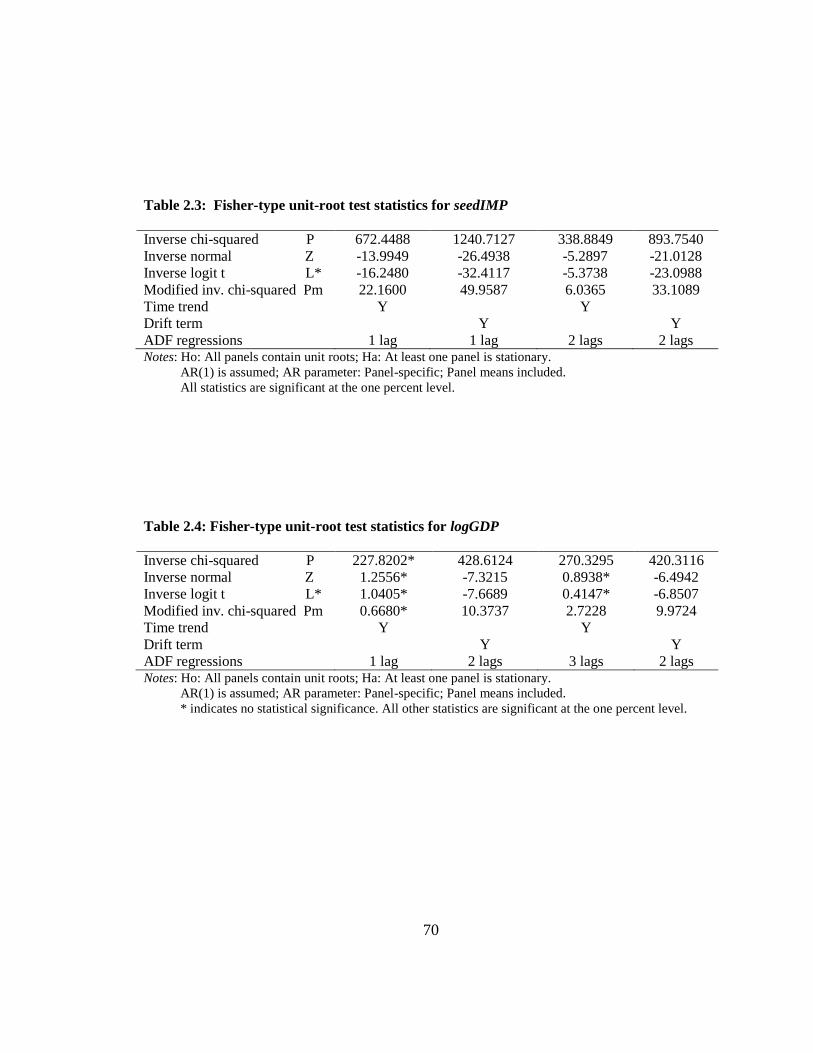
70

Table 2.3: Fisher-type unit-root test statistics for seedIMP

Inverse chi-squared P 672.4488 1240.7127 338.8849 893.7540

Inverse normal Z -13.9949 -26.4938 -5.2897 -21.0128

Inverse logit t L* -16.2480 -32.4117 -5.3738 -23.0988

Modified inv. chi-squared Pm 22.1600 49.9587 6.0365 33.1089

Time trend Y Y

Drift term Y Y

ADF regressions 1 lag 1 lag 2 lags 2 lags Notes: Ho: All panels contain unit roots; Ha: At least one panel is stationary.

AR(1) is assumed; AR parameter: Panel-specific; Panel means included.

All statistics are significant at the one percent level.

Table 2.4: Fisher-type unit-root test statistics for logGDP

Inverse chi-squared P 227.8202* 428.6124 270.3295 420.3116

Inverse normal Z 1.2556* -7.3215 0.8938* -6.4942

Inverse logit t L* 1.0405* -7.6689 0.4147* -6.8507

Modified inv. chi-squared Pm 0.6680* 10.3737 2.7228 9.9724

Time trend Y Y

Drift term Y Y

ADF regressions 1 lag 2 lags 3 lags 2 lags Notes: Ho: All panels contain unit roots; Ha: At least one panel is stationary.

AR(1) is assumed; AR parameter: Panel-specific; Panel means included.

* indicates no statistical significance. All other statistics are significant at the one percent level.

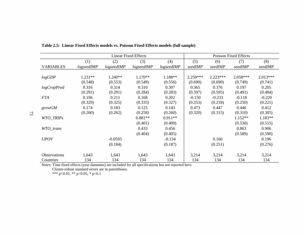
71

Table 2.5: Linear Fixed Effects models vs. Poisson Fixed Effects models (full sample)

Linear Fixed Effects Poisson Fixed Effects

(1) (2) (3) (4) (5) (6) (7) (8)

VARIABLES logseedIMP logseedIMP logseedIMP logseedIMP seedIMP seedIMP seedIMP seedIMP

logGDP 1.231** 1.240** 1.170** 1.188** 2.259*** 2.223*** 2.058*** 2.013*** (0.548) (0.553) (0.549) (0.556) (0.690) (0.690) (0.749) (0.741)

logCropProd 0.316 0.314 0.310 0.307 0.365 0.376 0.197 0.205 (0.291) (0.291) (0.284) (0.283) (0.597) (0.595) (0.491) (0.484)

FTA 0.196 0.211 0.168 0.202 -0.150 -0.233 -0.118 -0.220 (0.329) (0.325) (0.335) (0.327) (0.253) (0.218) (0.250) (0.221)

growGM 0.174 0.183 0.125 0.143 0.473 0.447 0.446 0.412 (0.260) (0.262) (0.258) (0.260) (0.320) (0.315) (0.310) (0.305)

WTO_TRIPs 0.881** 0.911** 1.152** 1.183**

(0.401) (0.409) (0.530) (0.515)

WTO_trans 0.433 0.456 0.863 0.906

(0.404) (0.405) (0.589) (0.590)

UPOV -0.0593 -0.134 0.160 0.196

(0.184) (0.187) (0.251) (0.276)

Observations 1,643 1,643 1,643 1,643 3,214 3,214 3,214 3,214 Countries 134 134 134 134 134 134 134 134 Notes: Time fixed effects (year dummies) are included for all specifications but not reported here.

Cluster-robust standard errors are in parentheses.

*** p<0.01, ** p<0.05, * p<0.1

71

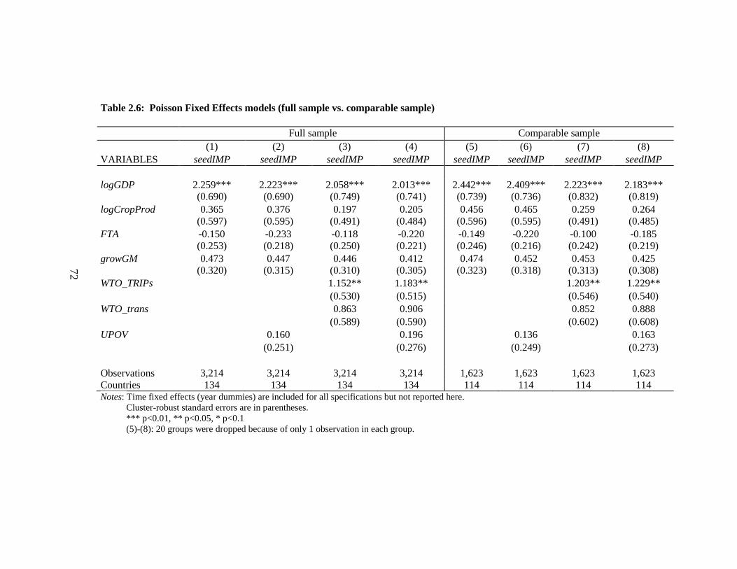
Table 2.6: Poisson Fixed Effects models (full sample vs. comparable sample)

Full sample Comparable sample

(1) (2) (3) (4) (5) (6) (7) (8)

VARIABLES seedIMP seedIMP seedIMP seedIMP seedIMP seedIMP seedIMP seedIMP

logGDP 2.259*** 2.223*** 2.058*** 2.013*** 2.442*** 2.409*** 2.223*** 2.183*** (0.690) (0.690) (0.749) (0.741) (0.739) (0.736) (0.832) (0.819)

logCropProd 0.365 0.376 0.197 0.205 0.456 0.465 0.259 0.264 (0.597) (0.595) (0.491) (0.484) (0.596) (0.595) (0.491) (0.485)

FTA -0.150 -0.233 -0.118 -0.220 -0.149 -0.220 -0.100 -0.185 (0.253) (0.218) (0.250) (0.221) (0.246) (0.216) (0.242) (0.219)

growGM 0.473 0.447 0.446 0.412 0.474 0.452 0.453 0.425 (0.320) (0.315) (0.310) (0.305) (0.323) (0.318) (0.313) (0.308)

WTO_TRIPs 1.152** 1.183** 1.203** 1.229**

(0.530) (0.515) (0.546) (0.540)

WTO_trans 0.863 0.906 0.852 0.888

(0.589) (0.590) (0.602) (0.608)

UPOV 0.160 0.196 0.136 0.163

(0.251) (0.276) (0.249) (0.273)

Observations 3,214 3,214 3,214 3,214 1,623 1,623 1,623 1,623 Countries 134 134 134 134 114 114 114 114 Notes: Time fixed effects (year dummies) are included for all specifications but not reported here.

Cluster-robust standard errors are in parentheses.

*** p<0.01, ** p<0.05, * p<0.1

(5)-(8): 20 groups were dropped because of only 1 observation in each group.

72

Table 2.7: Linear Fixed Effects models vs. Poisson Fixed Effects models (full sample, UPOV10, UPOV01, UPOV11)

Linear Fixed Effects Poisson Fixed Effects

(1) (2) (3) (4) (5) (6) (7) (8)

VARIABLES logseedIMP logseedIMP logseedIMP logseedIMP seedIMP seedIMP seedIMP seedIMP

logGDP 1.231** 1.387** 1.170** 1.316** 2.259*** 2.513*** 2.058*** 2.324*** (0.548) (0.538) (0.549) (0.539) (0.690) (0.662) (0.749) (0.748)

logCropProd 0.316 0.280 0.310 0.271 0.365 0.340 0.197 0.180 (0.291) (0.290) (0.284) (0.280) (0.597) (0.588) (0.491) (0.484)

FTA 0.196 0.280 0.168 0.270 -0.150 -0.253 -0.118 -0.221 (0.329) (0.300) (0.335) (0.303) (0.253) (0.200) (0.250) (0.202)

growGM 0.174 0.0916 0.125 0.0484 0.473 0.483 0.446 0.452 (0.260) (0.265) (0.258) (0.261) (0.320) (0.310) (0.310) (0.302)

UPOV10 0.244 0.173 0.275 0.278

(0.233) (0.234) (0.287) (0.306)

UPOV01 -0.663** -0.759** -0.210 -0.102

(0.286) (0.296) (0.354) (0.421)

UPOV11 0.369 0.241 0.946 0.890

(0.481) (0.485) (0.607) (0.622)

WTO_TRIPs 0.881** 0.924** 1.152** 1.046*

(0.401) (0.425) (0.530) (0.552)

WTO_trans 0.433 0.470 0.863 0.741

(0.404) (0.412) (0.589) (0.607)

Observations 1,643 1,643 1,643 1,643 3,214 3,214 3,214 3,214 Countries 134 134 134 134 134 134 134 134 Notes: Time fixed effects (year dummies) are included for all specifications but not reported here.

Cluster-robust standard errors are in parentheses.

*** p<0.01, ** p<0.05, * p<0.1

73

Table 2.8: Poisson Fixed Effects models (full sample vs. comparable sample, UPOV10, UPOV01, UPOV11)

Full sample Comparable sample

(1) (2) (3) (4) (5) (6) (7) (8)

VARIABLES seedIMP seedIMP seedIMP seedIMP seedIMP seedIMP seedIMP seedIMP

logGDP 2.259*** 2.513*** 2.058*** 2.324*** 2.442*** 2.796*** 2.223*** 2.600*** (0.690) (0.662) (0.749) (0.748) (0.739) (0.709) (0.832) (0.819)

logCropProd 0.365 0.340 0.197 0.180 0.456 0.423 0.259 0.235 (0.597) (0.588) (0.491) (0.484) (0.596) (0.585) (0.491) (0.483)

FTA -0.150 -0.253 -0.118 -0.221 -0.149 -0.246 -0.100 -0.196 (0.253) (0.200) (0.250) (0.202) (0.246) (0.197) (0.242) (0.202)

growGM 0.473 0.483 0.446 0.452 0.474 0.489 0.453 0.465 (0.320) (0.310) (0.310) (0.302) (0.323) (0.310) (0.313) (0.302)

UPOV10 0.275 0.278 0.267 0.267

(0.287) (0.306) (0.288) (0.314)

UPOV01 -0.210 -0.102 -0.307 -0.203

(0.354) (0.421) (0.328) (0.393)

UPOV78_91 0.946 0.890 0.982 0.934

(0.607) (0.622) (0.602) (0.620)

WTO_TRIPs 1.152** 1.046* 1.203** 1.078*

(0.530) (0.552) (0.546) (0.575)

WTO_trans 0.863 0.741 0.852 0.705

(0.589) (0.607) (0.602) (0.623)

Observations 3,214 3,214 3,214 3,214 1,623 1,623 1,623 1,623 Countries 134 134 134 134 114 114 114 114 Notes: Time fixed effects (year dummies) are included for all specifications but not reported here.

Cluster-robust standard errors are in parentheses.

*** p<0.01, ** p<0.05, * p<0.1

74

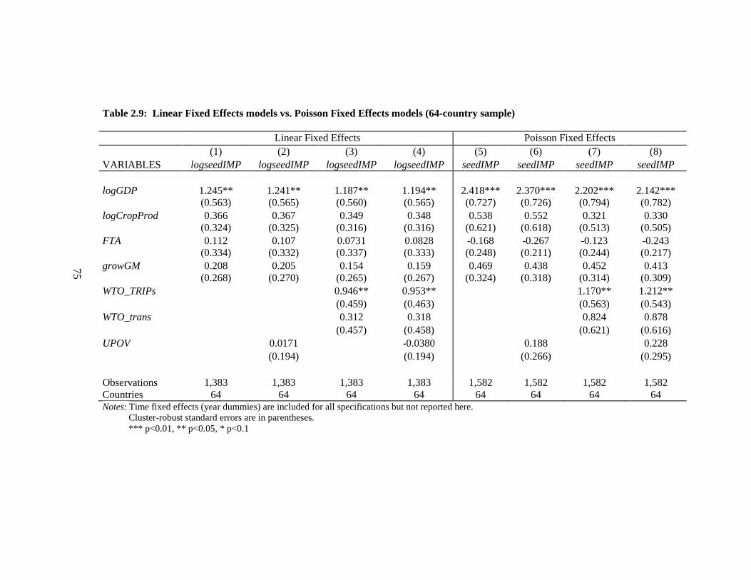
Table 2.9: Linear Fixed Effects models vs. Poisson Fixed Effects models (64-country sample)

Linear Fixed Effects Poisson Fixed Effects

(1) (2) (3) (4) (5) (6) (7) (8)

VARIABLES logseedIMP logseedIMP logseedIMP logseedIMP seedIMP seedIMP seedIMP seedIMP

logGDP 1.245** 1.241** 1.187** 1.194** 2.418*** 2.370*** 2.202*** 2.142*** (0.563) (0.565) (0.560) (0.565) (0.727) (0.726) (0.794) (0.782)

logCropProd 0.366 0.367 0.349 0.348 0.538 0.552 0.321 0.330 (0.324) (0.325) (0.316) (0.316) (0.621) (0.618) (0.513) (0.505)

FTA 0.112 0.107 0.0731 0.0828 -0.168 -0.267 -0.123 -0.243 (0.334) (0.332) (0.337) (0.333) (0.248) (0.211) (0.244) (0.217)

growGM 0.208 0.205 0.154 0.159 0.469 0.438 0.452 0.413 (0.268) (0.270) (0.265) (0.267) (0.324) (0.318) (0.314) (0.309)

WTO_TRIPs 0.946** 0.953** 1.170** 1.212**

(0.459) (0.463) (0.563) (0.543)

WTO_trans 0.312 0.318 0.824 0.878

(0.457) (0.458) (0.621) (0.616)

UPOV 0.0171 -0.0380 0.188 0.228

(0.194) (0.194) (0.266) (0.295)

Observations 1,383 1,383 1,383 1,383 1,582 1,582 1,582 1,582 Countries 64 64 64 64 64 64 64 64 Notes: Time fixed effects (year dummies) are included for all specifications but not reported here.

Cluster-robust standard errors are in parentheses.

*** p<0.01, ** p<0.05, * p<0.1

75

Table 2.10: Arellano-Bond estimator

Full Sample Trade Frequency > 18

(1) (2) (3) (4) (5) (6) (7) (8)

VARIABLES logseedIMP logseedIMP logseedIMP logseedIMP logseedIMP logseedIMP logseedIMP logseedIMP

L.logseedIMP 0.192*** 0.194*** 0.191*** 0.193*** 0.304*** 0.304*** 0.299*** 0.299*** (0.0710) (0.0706) (0.0694) (0.0689) (0.0875) (0.0869) (0.0850) (0.0845)

logGDP 1.858* 1.858 1.797 1.792 0.718 0.710 0.693 0.683 (1.127) (1.142) (1.141) (1.153) (1.139) (1.135) (1.137) (1.133)

logCropProd 0.697*** 0.698*** 0.694*** 0.694*** 0.862*** 0.861*** 0.851*** 0.849*** (0.184) (0.182) (0.185) (0.183) (0.225) (0.225) (0.232) (0.232)

FTA -0.747 -0.794 -0.743 -0.794 -0.842 -0.856 -0.843 -0.858 (0.538) (0.549) (0.536) (0.548) (0.548) (0.564) (0.545) (0.562)

growGM -0.0962 -0.107 -0.0924 -0.103 -0.178 -0.181 -0.175 -0.178 (0.242) (0.248) (0.241) (0.247) (0.165) (0.167) (0.166) (0.168)

WTO_TRIPs 0.346 0.368 1.129*** 1.139***

(0.533) (0.538) (0.356) (0.359)

WTO_trans 0.352 0.376 0.984*** 0.994***

(0.539) (0.539) (0.227) (0.231)

UPOV 0.198 0.217 0.0605 0.0637

(0.330) (0.337) (0.406) (0.407)

Arellano-Bond test Pass Pass Pass Pass Pass Pass Pass Pass Sargan test Pass Pass Pass Pass Pass Pass Pass Pass Observations 1,193 1,193 1,193 1,193 999 999 999 999 Countries 86 86 86 86 48 48 48 48 Notes: Time fixed effects (year dummies) are included for all specifications but not reported here.

Cluster-robust standard errors are in parentheses.

*** p<0.01, ** p<0.05, * p<0.1

76

Table 2.11: Arellano-Bond estimator (all regressors lagged once)

Full Sample Trade Frequency > 18

(1) (2) (3) (4) (5) (6) (7) (8)

VARIABLES logseedIMP logseedIMP logseedIMP logseedIMP logseedIMP logseedIMP logseedIMP logseedIMP

L.logseedIMP 0.188*** 0.189*** 0.189*** 0.190*** 0.302*** 0.302*** 0.306*** 0.306*** (0.0701) (0.0699) (0.0674) (0.0670) (0.0830) (0.0829) (0.0796) (0.0794)

logGDP 2.145 2.128 2.100 2.080 1.211 1.211 1.137 1.130 (1.365) (1.369) (1.368) (1.372) (1.576) (1.583) (1.565) (1.577)

L.logGDP -0.0725 -0.0561 -0.130 -0.106 -0.947 -0.961 -0.937 -0.953 (1.220) (1.223) (1.275) (1.279) (1.580) (1.574) (1.576) (1.563)

logCropProd 0.579*** 0.574*** 0.581*** 0.577*** 0.608*** 0.611*** 0.619*** 0.622*** (0.150) (0.152) (0.156) (0.160) (0.170) (0.172) (0.180) (0.183)

L.logCropProd -0.321* -0.321* -0.310* -0.309* -0.556** -0.552** -0.519** -0.514** (0.187) (0.186) (0.183) (0.183) (0.221) (0.219) (0.223) (0.221)

FTA -0.799 -0.839 -0.787 -0.833 -0.882 -0.896 -0.857* -0.879* (0.533) (0.545) (0.503) (0.520) (0.558) (0.573) (0.498) (0.523)

L.FTA 0.831*** 0.865*** 0.826*** 0.861*** 0.897*** 0.887*** 0.879*** 0.873** (0.288) (0.308) (0.289) (0.309) (0.320) (0.338) (0.322) (0.339)

growGM -0.0913 -0.104 -0.0853 -0.0994 -0.180 -0.185 -0.158 -0.166 (0.226) (0.234) (0.224) (0.232) (0.157) (0.157) (0.163) (0.161)

L.growGM -0.163 -0.158 -0.160 -0.156 -0.0116 -0.0165 0.000935 -0.00443 (0.190) (0.198) (0.190) (0.198) (0.226) (0.230) (0.222) (0.226)

WTO_TRIPs 0.364 0.384 1.106*** 1.110***

(0.558) (0.567) (0.386) (0.394)

L.WTO_TRIPs -0.206 -0.251 -0.586 -0.594

(0.683) (0.665) (1.238) (1.224)

WTO_trans 0.371 0.388 0.917*** 0.921***

(0.559) (0.554) (0.277) (0.276)

Continued

77

Table 2.11 continued

L.WTO_trans -0.151 -0.199 -0.423 -0.435

(0.643) (0.627) (1.205) (1.191)

UPOV 0.188 0.225 0.0576 0.0998

(0.321) (0.336) (0.393) (0.410)

L.UPOV -0.122 -0.129 0.0567 0.0429

(0.389) (0.391) (0.355) (0.369)

Arellano-Bond test Pass Pass Pass Pass Pass Pass Pass Pass Sargan test Pass Pass Pass Pass Pass Pass Pass Pass Observations 1,191 1,191 1,191 1,191 998 998 998 998 Countries 86 86 86 86 48 48 48 48 Notes: Time fixed effects (year dummies) are included for all specifications but not reported here.

Cluster-robust standard errors are in parentheses.

*** p<0.01, ** p<0.05, * p<0.1

78

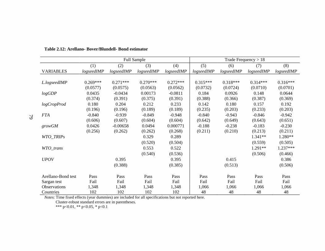
Table 2.12: Arellano- Bover/Blundell- Bond estimator

Full Sample Trade Frequency > 18

(1) (2) (3) (4) (5) (6) (7) (8)

VARIABLES logseedIMP logseedIMP logseedIMP logseedIMP logseedIMP logseedIMP logseedIMP logseedIMP

L.logseedIMP 0.269*** 0.271*** 0.270*** 0.272*** 0.315*** 0.318*** 0.314*** 0.316*** (0.0577) (0.0575) (0.0563) (0.0562) (0.0732) (0.0724) (0.0710) (0.0701)

logGDP 0.0435 -0.0434 0.00173 -0.0811 0.184 0.0926 0.148 0.0644 (0.374) (0.391) (0.375) (0.391) (0.388) (0.366) (0.387) (0.369)

logCropProd 0.180 0.204 0.212 0.233 0.142 0.180 0.157 0.192 (0.196) (0.196) (0.189) (0.189) (0.235) (0.203) (0.233) (0.203)

FTA -0.840 -0.939 -0.849 -0.948 -0.840 -0.943 -0.846 -0.942 (0.606) (0.607) (0.604) (0.604) (0.642) (0.649) (0.643) (0.651)

growGM 0.0426 -0.00658 0.0494 0.000771 -0.188 -0.238 -0.183 -0.230 (0.256) (0.262) (0.262) (0.268) (0.211) (0.210) (0.213) (0.211)

WTO_TRIPs 0.329 0.289 1.341** 1.280**

(0.520) (0.504) (0.559) (0.505)

WTO_trans 0.553 0.522 1.291** 1.237***

(0.540) (0.536) (0.506) (0.466)

UPOV 0.395 0.395 0.415 0.386

(0.388) (0.385) (0.513) (0.506)

Arellano-Bond test Pass Pass Pass Pass Pass Pass Pass Pass Sargan test Fail Fail Fail Fail Fail Fail Fail Fail Observations 1,348 1,348 1,348 1,348 1,066 1,066 1,066 1,066 Countries 102 102 102 102 48 48 48 48

Notes: Time fixed effects (year dummies) are included for all specifications but not reported here.

Cluster-robust standard errors are in parentheses.

*** p<0.01, ** p<0.05, * p<0.1

79

Table 2.13: Arellano- Bover/Blundell- Bond estimator (all regressors lagged once)

Full Sample Trade Frequency >18

(1) (2) (3) (4) (5) (6) (7) (8)

VARIABLES logseedIMP logseedIMP logseedIMP logseedIMP logseedIMP logseedIMP logseedIMP logseedIMP

L.logseedIMP 0.276*** 0.277*** 0.278*** 0.280*** 0.328*** 0.329*** 0.329*** 0.330*** (0.0541) (0.0542) (0.0519) (0.0520) (0.0683) (0.0682) (0.0672) (0.0670)

logGDP 1.225 1.179 1.213 1.154 1.032 1.064 0.975 0.999 (1.313) (1.307) (1.308) (1.301) (1.562) (1.543) (1.551) (1.533)

L.logGDP -0.903 -0.907 -0.912 -0.901 -0.633 -0.744 -0.605 -0.707 (1.260) (1.262) (1.255) (1.252) (1.508) (1.484) (1.513) (1.481)

logCropProd 0.509*** 0.516*** 0.514*** 0.519*** 0.642*** 0.657*** 0.639*** 0.654*** (0.168) (0.169) (0.160) (0.160) (0.192) (0.184) (0.193) (0.186)

L.logCropProd -0.553*** -0.543*** -0.543*** -0.534*** -0.713*** -0.692*** -0.693*** -0.672*** (0.173) (0.171) (0.179) (0.177) (0.215) (0.201) (0.210) (0.195)

FTA -1.031* -1.100* -1.033* -1.108* -1.146* -1.189* -1.125* -1.171* (0.591) (0.602) (0.570) (0.581) (0.644) (0.659) (0.588) (0.609)

L.FTA 0.998*** 1.024*** 0.987*** 1.014*** 1.029*** 0.973** 1.013*** 0.962** (0.358) (0.372) (0.361) (0.374) (0.394) (0.402) (0.389) (0.396)

growGM 0.0249 -0.00166 0.0360 0.00743 -0.160 -0.184 -0.137 -0.162 (0.235) (0.239) (0.237) (0.242) (0.186) (0.186) (0.191) (0.189)

L.growGM -0.0659 -0.0815 -0.0786 -0.0947 0.0348 0.00240 0.0393 0.00703 (0.249) (0.247) (0.249) (0.247) (0.250) (0.242) (0.248) (0.240)

WTO_TRIPs 0.238 0.244 1.159** 1.122***

(0.508) (0.523) (0.465) (0.435)

L.WTO_TRIPs -0.166 -0.239 -0.487 -0.543

(0.551) (0.545) (1.141) (1.137)

WTO_trans 0.477 0.481 1.057*** 1.027***

(0.516) (0.523) (0.393) (0.373)

Continued

80

Table 2.13 continued

L.WTO_trans -0.191 -0.264 -0.356 -0.409

(0.525) (0.515) (1.118) (1.106)

UPOV 0.309 0.343 0.174 0.199

(0.346) (0.357) (0.415) (0.433)

L.UPOV -0.102 -0.108 0.174 0.154

(0.414) (0.419) (0.399) (0.409)

Arellano-Bond test Pass Pass Pass Pass Pass Pass Pass Pass Sargan test Fail Fail Fail Fail Pass* Pass* Pass* Pass* Observations 1,345 1,345 1,345 1,345 1,064 1,064 1,064 1,064 Countries 102 102 102 102 48 48 48 48 Notes: Time fixed effects (year dummies) are included for all specifications but not reported here.

Cluster-robust standard errors are in parentheses.

*** p<0.01, ** p<0.05, * p<0.1

Pass*- reject at the 10 percent level

81

82

References

Acs, Z. J. and D. B. Audretsch. “Innovation in large and small firms: an empirical

analysis,” American Economic Review 78 (1988): 678-690.

Acs, Z. J., D. B. Audretsch, and M. P. Feldman. “R&D spillovers and innovative

activity,” Managerial and Decision Economics 15 (1994a): 131-138.

Acs, Z. J., D. B. Audretsch, and M. P. Feldman. “R&D spillovers and recipient firm

size,” Review of Economics and Statistics 76 (1994b): 336-340.

Anderson, J. “A theoretical foundation for the gravity equation,” American Economic

Review 69 (1979): 106-116.

Anderson, J. “The gravity model,” Annual Review of Economics 3 (2011): 133-160.

Anderson, J. and E. van Wincoop. “Gravity with gravitas: A solution to the border

puzzle,” American Economic Review 93 (2003): 170-192.

Arellano, M. and S. Bond. “Some tests of specification for panel data: Monte Carlo

evidence and an application to employment equations,” Review of Econometric

Studies 58 (1991): 277–297.

Arellano, M. and O. Bover. “Another look at the instrumental variable estimation of

error-components models,” Journal of Econometrics 68 (1995): 29-51.

Arrow, K. J. “Economic welfare and the allocation of resources for inventions,” in The

Rate and Direction of Inventive Activity: Economic and Social Factors, R. R.

Nelson (ed.), Princeton, NJ: Princeton University Press (1962).

Atkinson, R. D. and Ezell, S. J. Innovation economics: the race for global advantage.

New Haven: Yale University Press (2012).

Audretsch, D. B. and M. P. Feldman. “R&D spillovers and the geography of innovation

and production,” American Economic Review 86 (1996): 630-640.

83

Ayyagaria1, M., A. Demirgüç-Kunta, and V. Maksimovica. “Firm innovation in

emerging markets: the role of finance, governance, and competition,” Journal of

Financial and Quantitative Analysis 46 (2011): 1545-1580.

Bagella, M. and Becchetti, L. “The ‘geographical agglomeration-private R&D

expenditure’ effect: empirical evidence on Italian data,” Economics of Innovation

and New Technology 11 (2002): 233–247.

Baldwin, R. “Hysteresis in trade,” mimeo prepared for NBER Summer Institute,

International Studies (1986).

Baptista R. and P. Swann. “Do firms in clusters innovate more?” Research Policy 27

(1998): 525-540.

Baumol, W. J. “Entrepreneurship and innovation: The (Micro) theory of price and profit,”

unpublished paper (2007).

Beaudry, C. “Entry, growth, and patenting in industrial clusters: a study of the aerospace

industry in the UK,” International Journal of the Economics of Business 8 (2001):

405–435.

Beaudry, C. and S. Breschi. “Does ‘Clustering’ really help firms’ innovative activities?”

CESPRI Working Paper 111 (2000).

Beaudry, C. and S. Breschi. “Are firms in clusters really more innovative?” Economics of

innovation and New Technology 12 (2003): 325-342.

Bergstrand, J. H. “The generalized gravity equation, monopolistic competition, and the

factor-proportions theory in international trade,” Review of Economics and

Statistics 71 (1989): 143-153.

Bergstrand, J. “The gravity equation in international trade: some microeconomic

foundations and empirical evidence,” Review of Economics and Statistics 67

(1985): 474-481.

Berle, A. A. and G. G. C. Means. The Modern Corporation and Private Property. New

York: Commerce Clearing House (1932).

Blundell, R. and S. Bond. “Initial conditions and moment restrictions in dynamic panel

data models,” Journal of Econometrics 87 (1998): 115-143.

Blundell, R., R. Griffith, and F. Windmeijer. “Individual effects and dynamics in count

data models,” Journal of Econometrics 108 (2002): 113-131.

84

Brambilla, I. “Multinationals, technology, and the introduction of varieties of goods.”

Journal of International Economics 79 (2009): 89-101.

Bun, M. and F. Klaassen. “The importance of dynamics in panel gravity models of

trade,” unpublished paper, University of Amsterdam (2002).

Cameron, A. C. and P. K. Trivedi. Microeconometrics Using Stata. College Station, TX:

Stata Press (2009).

Chan, T., E. K. Y. Chen, and S. Chin. “China’s special economic zones: ideology, policy

and practice,” in China’s Special Economic Zones: Policies, Problems and

Prospects, Y. C. Jao and C. K. Leung (eds.), Hong Kong: Oxford University Press

(1986).

Cohen, W. M. “Fifty years of empirical studies of innovative activity and performance”

in vol. 1 of Handbook of The Economics of Innovation, B. H. Hall and N.

Rosenberg (eds.) Amsterdam: Elsevier (2010).

Cohen, W. M. and Klepper, S. “A reprise of size and R&D,” Economic Journal 106

(1996): 925-951.

Cohen, W. M. and R. C. Levin. “Empirical studies of innovation and market structure,”

in vol. 2 of Handbook of Industrial Organization, R. Schmalensee and R. W.

Amsterdam (eds.), New York: North-Holland (1989).

Deardorff, A. “Determinants of bilateral trade: Does gravity work in a neoclassical

world?” in The Regionalization of the World Economy, J. A. Frankel (ed.),

Chicago: University of Chicago Press (1998).

Démurger, S., J. D. Sachs, W. T. Woo, S. Bao, G. Chang, and A. Mellinger. “Geography,

economic policy, and regional development in China,” Asian Economic Papers 1

(2002): 146-197.

Dickey, D. A. and W. A. Fuller, “Distribution of the estimators for autoregressive time

series with a unit root,” Journal of the American Statistical Association 74 (1979):

427–431.

Dosi, G. and R. R. Nelson. “Technical change and Industrial dynamics as evolutionary

process” in vol. 1 of Handbook of The Economics of Innovation, B. H. Hall and

N. Rosenberg (eds.) Amsterdam: Elsevier (2010).

Eaton, D. “Trade and intellectual property rights in the agricultural seed sector,” paper

presented at the International Association of Agricultural Economists Conference,

Beijing, China, August 16-22 (2009).

85

Eisenhardt, K. “Agency theory: An assessment and review,” Academy of Management

Review, 14 (1989): 57-74.

Evenett, S. J. and W. Keller. “On theories explaining the success of the gravity equation,”

Journal of Political Economy 110 (2002): 281-316.

Fagerberg, J., M. Srholec, and B. Verspagen. “Innovation and economic development” in

vol. 2 of Handbook of The Economics of Innovation, B. H. Hall and N. Rosenberg

(eds.) Amsterdam: Elsevier (2010).

Feenstra, R. C. Advanced International Ttrade: Theory and Evidence. Princeton, NJ:

Princeton University Press (2004).

Feldman, M. P. The Geography of Innovation. Boston, MA: Springer (1994).

Feldman, M. P. and D. F. Kogler. “Stylized facts in the geography of innovation” in vol.

1 of Handbook of The Economics of Innovation, B. H. Hall and N. Rosenberg

(eds.) Amsterdam: Elsevier (2010).

Femandez-Cornejo, J. “The seed industry in US agriculture - an exploration of data and

information on crop seed markets, regulation, industry structure, and research and

development,” Agriculture Information Bulletin 786, Washington DC: Economic

Research Service, US Department of Agriculture (2004).

Ferrantino, M. J. “The effect of intellectual property rights on international trade and

investment,” Review of World Economics 129 (1993): 300-331.

Food and Agriculture Organization of the United Nations (FAO). The State of Food

Insecurity in the World. Rome: FAO (2012).

Galushko, V. "Do stronger intellectual property rights promote seed exchange: Evidence

from US seed exports?" Agricultural Economics 43 (2012): 59-71.

Gertler, M. S. “Tacit knowledge and the economic geography of context, or the

undefinable tacitness of being (there),” Journal of Economic Geography 3 (2003):

75-99.

Ginarte, J. C. and W. G. Park. “Determinants of patent rights: A cross-national study,”

Research Policy 26 (1997): 283-301.

Glaeser, E. “Introduction,” in Agglomeration Economies, E. Glaeser (ed.), Chicago:

University of Chicago Press (2010).

86

Gordon, I. R. and P. McCann. “Innovation, agglomeration, and regional development,”

Journal of Economic Geography 5 (2005): 523-543.

Grossman, G. M. and E. Helpman. “Trade, innovation, and growth,” American Economic

Review 80 (1990): 86-91.

Grossman, G. M. and E. Helpman. “Technology and trade,” in vol. 3 of Handbook of

International Economics, G. M. Grossman and K. Rogoff (eds.), Amsterdam:

North-Holland (1995).

Grossman, G. M. and E. L.-C. Lai. “International protection of intellectual property,”

American Economic Review 94 (2004): 1635-1653.

Hall, B. H and J. Lerner. “The financing of R&D and innovation,” in vol. 1 of Handbook

of The Economics of Innovation, B. H. Hall and N. Rosenberg (eds.) Amsterdam:

Elsevier (2010).

Harrison, B., M. R. Kelly, and J. Gant. “Innovative firm behavior and local milieu:

exploring the intersection of agglomeration, firm effects, and technological

change,” Economic Geography 72 (1996): 233–257.

Heckman, J. “Sample selection bias as a specification error,” Econometrica 47 (1979):

153-161.

Helpman, E., M. Melitz, and Y. Rubinstein. “Estimating trade flows: Trading partners

and trading volumes,” Quarterly Journal of Economics 123 (2008): 441-487.

Howard, P. H. “Visualizing consolidation in the global seed industry: 1996–2008,”

Sustainability 1 (2009): 1266-1287.

International Union for the Protection of New Varieties of Plants (UPOV). “Responding

to the challenges of a changing world: The role of new plant varieties and high

quality seed in agriculture,” Proceedings of the Second World Seed Conference,

Rome, Italy, September 8-10 (2009).

Ivus, O. “Do stronger patent rights raise high-tech exports to the developing world?”

Journal of International Economics 81 (2010): 38-47.

Jacobs, J. The Economy of Cities. New York: Vintage (1969).

Jaffe, A. B. “Real effects of academic research,” American Economic Review 79 (1989):

957-970.

87

Jaffe, A. B., M. Trajtenberg, and R. Henderson. “Geographic localization of knowledge

spillovers as evidenced by patent citations,” The Quarterly Journal of Economics

108 (1993): 577-598.

James, C. Global Status of Commercialized Biotech/GM Crops. ISAAA Brief 43 (2011).

Jayasinghe, S., J. C. Beghin and G. Moschini. “Determinants of world demand for U.S.

corn seeds: The role of trade costs,” American Journal of Agricultural Economics

92(2010): 999-1010.

Kaufmann, D., A. Kraay, and M. Mastruzzi. Governance matters VIII: aggregate and

individual governance indicators, 1996-2008. World Bank policy research

working paper 4978 (2009).

Keller, W. “International technology diffusion”, Journal of Economic Literature (2004):

752–782.

Kesan, J. P. and A. A. Gallo. “Insecure property rights and plant varieties: The effects on

the market for seeds and on farmers in Argentina,” in Agricultural Biotechnology

and Intellectual Property: Seeds of Change, J. P. Kesan (ed.), Wallingford, UK:

CABI (2007).

Lee, C. “Do firms in clusters invest in R&D more intensively? Theory and evidence from

multi-country data,” Research Policy 38 (2009): 1159-1171.

Lee, P. M. and H. M. O’Neill. “Ownership structures and R&D investments of U.S. and

Japanese firms: Agency and stewardship perspectives,” Academy of Management

Journal 46 (2003): 212-225.

Lesser, W. H. “Plant breeders’ rights: an introduction” in Intellectual Property

Management in Health and Agricultural Innovation: A Handbook of Best

Practices, A. Krattiger, R. T. Mahoney, L. Nelsen, et al. (eds.) Davis, CA: PIPRA

(2007).

Mairesse, J. and P. Mohnen. “Using innovation surveys for econometric analysis,” in vol.

1 of Handbook of The Economics of Innovation, B. H. Hall and N. Rosenberg

(eds.) Amsterdam: Elsevier (2010).

Malmberg, A. and P. Maskell. "Localized learning revisited." Growth and Change 37

(2006): 1-18.

Marshall, A. Principles of Economics. New York: Macmillan and Company (1890).

88

Maskus, K. E. and M. Penubarti. “How trade-related are intellectual property rights?”

Journal of International Economics 39 (1995): 227-248.

OECD. Oslo Manual (3rd

ed.) Paris: OECD (2005).

Olivero, M. P. and Y. V. Yotov. “Dynamic gravity: endogenous country size and asset

accumulation.” Canadian Journal of Economics 45 (2012): 64-92.

Park, W. G. “International patent protection: 1960–2005,” Research Policy 37 (2008):

761-766.

Pavitt, K. and P. Patel. “Global corporations and national systems of innovation: who

dominates whom,” in Innovation Policy in a Global Economy, D. Archibugi, J.

Howells and J. Michie (eds.), Cambridge, MA: Cambridge University Press

(1999): 94-119.

Porter, M. E. The Competitive Advantage of Nations. New York: Free Press (1990).

Sargan, J. D. “The estimation of economic relationships using instrumental variables,”

Econometrica 26 (1958): 393-415.

Saxenian, A. Regional Advantage: Culture and Competition in Silicon Valley and Route

128. Cambridge, MA: Harvard University Press (1994).

Schumpeter, J. A. Capitalism, Socialism and Democracy. New York: Harper & Row

(1942).

Silva, J. and S. Tenreyro. “The log of gravity,” Review of Economics and Statistics 88

(2006): 641-658.

Singh, O. V., S. Ghai, D. Paul, and R. K. Jain. “Genetically modified crops: Success,

safety assessment, and public concern,” Applied Microbiology and Biotechnology

71 (2006): 598-607.

Smith, P. J. “Are weak patent rights a barrier to US exports?” Journal of International

Economics 48 (1999): 151-177.

Stoneman, P. The Handbook of Economics of Innovation and Technological Change,

Cambridge, MA: Blackwell (1995).

Swann, G.M.P. The economics of innovation: an introduction. Cheltenham : Edward

Elgar (2009).

89

Tinbergen, J. “An analysis of world trade flows,” in Shaping the World Economy, J.

Tinbergen (ed.), New York: Twentieth Century Fund (1962).

Walcott, S. M. Chinese Science and Technology Industrial Parks. Burlington, VT:

Ashgate (2003).

Wang, J. “Industrial clusters in China: the low road versus the high road in cluster

development,” in Development on the Ground: Clusters, Networks and Regions in

Emerging Economies, A. J. Scott and G. Garofoli (eds.), New York: Routledge

(2007).

Wang, W. “Innovation enables sustainable development in China,” Chinese Journal of

Population Resources and Environment 10 (2012): 5-6.

Westerlund, J. and F. Wilhelmsson. “Estimating the gravity model without gravity using

panel data,” Applied Economics 43 (2011): 641-649.

Windmeijer, F, and J. M. C. Santos Silva. “Endogeneity in count data models: an

application to demand for health care.” Journal of Applied Econometrics 12

(1997): 281-294.

Windmeijer, F. “ExpEnd, a Gauss programme for non-linear GMM estimation of

exponential models with endogenous regressors for cross section and panel data.”

The Institute for Fiscal Studies, Department of Economics, University of College

London, Cemmap Working Paper, CWP14/02 (2002).

Wooldridge, J. M. Econometric Analysis of Cross Section and Panel Data. Cambridge,

MA: MIT Press (2002).

Xu, C. "The fundamental institutions of China’s reforms and development," Journal of

Economic Literature 49 (2011): 1076-1151.

Yang, C. H. and R. J. Woo. “Do stronger intellectual property rights induce more

agricultural trade? A dynamic panel data model applied to seed trade,”

Agricultural Economics 35 (2006): 91-101.

Zeng, D. Z. “How do special economic zones and industrial clusters drive China’s rapid

development?” World Bank Policy Research Working Paper 5583 (2011).

Zhang, C., D. Z. Zeng, W. P. Mako, and J. Seward. Promoting Enterprise-led Innovation

in China. Washington, DC: The World Bank (2009).