Essays on Inequality of Opportunity

in

Health and Human Development

João Pedro Cordas da Rosa Dias

Ph.D. Thesis

The University of York

Department of Economics and Related Studies

May 2010

2

Abstract This thesis comprises four essays on inequality of opportunity in health and human development. Chapter 2 proposes an empirical implementation of the concept of inequality of opportunity in health and applies it to data from the UK National Child Development Study. Drawing on the distinction between circumstance and effort variables in John Roemer's work on equality of opportunity, circumstances are proxied by parental socio-economic status and childhood health; effort is proxied by health-related lifestyles and educational attainment. Stochastic dominance tests are used to detect inequality of opportunity in the conditional distributions of self-assessed health in adulthood. Alternative measures of inequality of opportunity are proposed. Parametric models are estimated to quantify the triangular relationship between circumstances, effort and health. The results indicate considerable and persistent inequality of opportunity in health. Circumstances affect health in adulthood both directly and through effort factors such as educational attainment, suggesting complementary educational policies may be important for reducing health inequalities. Chapter 3 specifies a behavioural model of inequality of opportunity in health that integrates John Roemer’s framework of inequality of opportunity with the Grossman model of health capital and demand for health. The model generates a recursive system of equations for health and lifestyles, which is jointly estimated by full information maximum likelihood with freely correlated error terms. The analysis innovates by accounting for unobserved heterogeneity, thereby addressing the partial-circumstance problem, and by extending the analysis to health outcomes other than self-assessed health, namely long standing illness, disability and mental health. Chapter 4 explores the existence of long-term health returns to different qualities of education, and examines the role of quality of schooling as a source of inequality of opportunity in health. It provides corroborative evidence of a statistically significant and economically sizable association between quality of education and a number of health and health-related outcomes that remains valid beyond the effects of measured ability, social development and academic qualifications. The results also establish quality of schooling as a leading source of inequality of opportunity in health. Chapter 5 exploits a natural experiment provided by the fact that cohort-members attended different types of secondary school, as their schooling lay within the transition period of the comprehensive education reform in England and Wales that commenced in the 1960’s. This experiment is used to explore the impact of educational attainment and of school quality on health and health-related behaviour later in life. A combination of matching methods, parametric regressions, and instrumental variable approaches are used to deal with selection effects and to evaluate differences in adult health outcomes and health-related behaviour for cohort members exposed to the old (selective) and to the new (comprehensive) educational systems.

3

Contents

Abstract 2

Acknowledgements 8

Declaration 9

Chapter 1

Introduction 10

Chapter 2

Inequality of Opportunity in Health: Evidence from a UK Cohort Study 17 2.1 Introduction 17 2.2 Background 18

2.2.1 Equality of Opportunity: the Roemer model 18 2.2.2 Definitions and testable conditions 21 2.2.3 Measures of inequality of opportunity 22 2.2.3.1 The Gini-opportunity index 23 2.2.3.2 An alternative approach 24

2.3. Data 26 2.3.1 The National Child Development Study (NCDS) 26 2.3.2 Variables: health, circumstances and effort 27

2.4 Testing and measuring inequality of opportunity in health 29 2.5 Estimation results 31

2.5.1 Adult health and early life circumstances: direct and indirect effects 31 2.5.2 Circumstances and effort: primary pathways 34

2.6 Conclusions 36 Appendix A 38

Chapter 3

Modelling Opportunity in Health under Partial Observability of Circumstances 44

3.1 Introduction 44 3.2 Equality of opportunity: the Roemer model in the context of health 45 3.3 Outline of the structural model 47 3.4 Data 49 3.5 Methods 52 3.6 Results 53 3.7 Discussion and conclusions 58 Appendix B 60

Chapter 4

Quality of Schooling and Inequality of Opportunity in Health 62 4.1 Introduction 62 4.2 Quality of schooling 64

4.2.1 Primary education 64 4.2.2 Secondary education: the comprehensive reform and equality of opportunity 64

4.3 Data 65 4.3.1 Childhood health, parental background and neighbourhood characteristics 65 4.3.2 Cognitive ability, social development and educational achievement 66 4.3.3 Health-related behaviours, attitudes and outcomes 67 4.3.4 Sample selection and non-response 68

4.4 Methods 69 Inequality of opportunity in health 69

4

4.4.2 Regression analysis 70 4.5 Results 71

4.5.1 Quality of schooling and inequality of opportunity in health 71 4.5.2 Quality of schooling, health and lifestyle: primary schools 72 4.5.3 Quality of schooling, health and lifestyle: secondary schools 74

4.6 Conclusions 76 Appendix C 78

Chapter 5

The Impact of Childhood Cognitive Skills, Social Adjustment and Schooling on Adult Health and Lifestyle 90

5.1 Introduction 90 5.2 Comprehensive schooling reforms and the 1958 cohort 94 5.3 NCDS data and study design 96

5.3.1 Childhood health and parental background 98 5.3.2 Cognitive ability, non-cognitive skills and social adjustment 98 5.3.3 Local area characteristics 101 5.3.4 Educational attainment and quality of schooling 102 5.3.5 Intermediate outcomes: health-related behaviours 103 5.3.6 Main outcomes: adult health 104

5.4 Sample selection and balanced samples 106 5.4.1 Sample selection and non-response 106 5.4.2 Balance of covariates between selective and non-selective schools 107 5.4.3 ‘Coaching effects’: absolute and relative cognitive ability 111 5.4.4 Matched sub-samples 113

5.5 Econometric models and results 116 5.5.1 Pre-schooling characteristics 116 5.5.2 The impact of attainment and quality of schooling with controls for observables 118 5.5.3 Instrumental variables estimates 119 5.5.4 Heterogeneous effects by type of school 121

5. 6 Discussion 123 Appendix D 126

Chapter 6

Conclusions 127

Bibliography 132

 

5

List of tables

Chapter 2

Table 1: Summary statistics 38

Table 2: Tests of stochastic dominance between types 39

Table 3: Measures of inequalty of opportunity 40

Table 4: Adult health and circumstances 41

Table 5: Adult health, circumstances and effort 42

Table 6: The impact of circumstances on effort 43

Chapter 3

Table 1: System erros correlation matrix 60

Table 2: System estimates 61

Chapter 4

Table 1: NCDS cohort-members by type of primary school 78

Table 2: Secondary school characteristics 79

Table 3: Estimation sample vs full sample 80

Table 4: Quality of primary schooling, health and health-related

behaviours 81

Table 5: Quality of secondary schooling, health and health-related

behaviours 82

Table 6: Stochastic dominance tests for inequality of opportunity

in health 83

Chapter 5

Table 1: Characteristics of different types of schools

(as attended by NCDS cohort at age 16) 95

Table 2: Educational attainment: highest secondary qualification 102

Table 3: Breakdown of long-standing illness (LSI) by percentage with

specific main conditions (ICD-9) 105

Table 4: Sample means for outcomes 106

6

Table 5: Sample means for type of schooling and cognitive ability 107

Table 6: Percentage bias before and after pruning and matching

for key covariates 108

Table 7: Regressions for cognitive ability scores at ages 7 and 11:

full sample 113

Table 8: Percentage bias before and after pruning and matching

for key covariates: sub-sample of grammar and comprehensive

pupils 114

Table 9: Percentage bias before and after pruning and matching

for key covariates: sub-sample of secondary modern and

comprehensive pupils 114

Table 10: Selected regression results for pre-schooling characteristics

and health-related behaviours 116

Table 11: Selected regression results for pre-schooling characteristics

and health outcomes 117

Table 12: Effect of educational attainment and quality of schooling on

health-related behaviours 118

Table 13: Effect of educational attainment and quality of schooling on

health outcomes 119

Table 14 Effect of educational attainment on health-related behaviours:

IV estimates 120

Table 15: Effect of educational attainment on health outcomes:

IV estimates 121

Table 16: Effect of educational attainment on health-related behaviours:

matched sample of grammar and comprehensive pupils 122

Table 17: Effect of educational attainment on health-related behaviours:

matched sample of secondary modern and comprehensive

pupils 122

Table 18: Effect of educational attainment on health outcomes:

matched sample of grammar and comprehensive pupils 123

Table 19: Effect of educational attainment on health outcomes:

matched sample of secondary modern and comprehensive

pupils 123

7

List of figures  

Chapter 2

Figure 1: SAH (age 46) by parental socioeconomic group 39 Chapter 4

Figure 1: NCDS cohort-members by type of school (age 16) 84

Figure 2: Distribution of pupil-teacher ratios by type of primary

school 85

Figure 3: Distribution of pupil-teacher ratios by type of secondary

school 86

Figure 4: Distributions of cognitive and non-cognitive in the NCDS

cohort 87

Figure 5: Stochastic dominance: empirical distributions of SAH (age 46)

by type of secondary school 88

Figure 6: Stochastic dominance: empirical distributions of mental

illness (age 46) by type of secondary school 89

Chapter 5

Figure 1: Schematic view of study design and NCDS variables 97

Figure 2: Empirical distributions of cognitive ability scores by type

of school 100

Figure 3: Empirical density of Bristol Social Adjustment Guide

(BSAG) 101

Figure 4: Empirical QQ-plots for cognitive score at 7 and BSAG score:

before and after matching 109

Figure 5: Distribution of propensity score over selective (“untreated”)

and non-selective (“treated”) schools 111

Figure 6: Empirical distributions of relative ability by type of school 112

8

Acknowledgements

I would like to extend my gratitude to my thesis advisors Andrew Jones, Nigel Rice

and Peter Smith for providing outstanding guidance throughout my PhD. I would

also like to thank the Centre for Health Economics, especially the members of the

Health Econometrics and Data Group for invaluable encouragement and

camaraderie. Funding by Fundação para a Ciência e a Tecnologia is gratefully

acknowledged.

Very special thanks go to Dimitra for her loving support and understanding.

I dedicate this thesis to my parents.

9

Declaration

I confirm that the work presented in this thesis is my own, except where co-

authorship is explicitly acknowledged.

Chapter 2 has been published as a single authored peer-reviewed research article

under the title: Inequality of opportunity in health: evidence from a UK cohort

study. Health Economics 2009; 18(9):1057-74.

Chapter 3 has also been published as a single authored peer-reviewed research

paper under the title: Modelling opportunity in health under partial observability of

circumstances. Health Economics 2010; 19(3):252-64. During the Seventh World

Congress of the International Health Economics Association (iHEA), held in

Beijing in July 2009, an earlier version of this paper was awarded the prize of the

iHEA student competition “Young Researchers in Health Economics”. Candidates

were asked to submit full papers, which were judged by a competition committee

made up of Alistair McGuire (Chair), Terkel Christiansen, Bruce Hollingsworth, and

Hu Shanlian.

Chapter 4 is written in co-authorship with Professor Andrew Jones and Professor

Nigel Rice. I am the lead author, having identified the theme of research and the

original idea, prepared the data, carried out the empirical analysis and written the

first draft.

Chapter 5 is also written in co-authorship with Professor Andrew Jones and

Professor Nigel Rice. I contributed to the original research idea and to the choice of

methodological approach, prepared the data, performed part of the empirical

analysis and contributed towards the elaboration of the first draft. This research

paper is currently under review for publication in a peer-reviewed journal.

Preliminary versions of chapters 4 and 5 have been presented at the University of

Chicago, University of Lausanne, University of Manchester, University of Paris

Descartes, McMaster University, University of Wisconsin-Madison, University of

Coimbra and Korea University.

10

Chapter 1

Introduction This thesis consists of a collection of four essays on inequality of opportunity. It is

motivated by recent advances in the theory of distributive justice and contributes

towards an integrated normative analysis of inequalities in health, education and

other aspects of human development.

As asserted by Roemer (2005), equality of opportunity is to be contrasted with

equality of outcomes. The Achilles' heel of the advocacy of equality of outcomes

has traditionally been its failure to hold individuals accountable for their choices. In

light of this, the greatest recent progress in the egalitarian theory of justice, as

Cohen (1989) puts it, is arguably the co-option of the sharpest idea in the anti–

egalitarian arsenal: the notion of responsibility. By compensating for the impact of

circumstances beyond individual control, yet holding individuals responsible for the

consequences of their choices, equality of opportunity is an appealing compromise

between strict equality of outcomes and mere equity of formal rights. It has thus

attracted growing attention in the economics literature and is being increasingly

advocated by policy makers, as is made clear in The World Bank Development

Report 2006, Equity and Development, which focuses on the inequality issue (World

Bank, 2005).

This conceptual progress is the culmination of a series of developments in political

philosophy. Rawls’ (1971) pioneering work is credited with reinventing egalitarian

justice. Together with Amartya Sen’s concept of equality of capabilities, Rawls’

equality of social primary goods replaces subjective utility with an objective criterion.

Once these goods and capabilities are equally distributed, any residual inequality is

deemed a legitimate consequence of individual choice, hence of individual

responsibility. As Barry (1991) makes clear, between the polar extremes of the choicist

position, which attributes every individual outcome to free and unconstrained

choice, and the anti-choicist argument, which views outcomes as the reflection of

differences in the circumstances that determine choices, there are infinite

11

intermediate positions. Dworkin (1981; 2000) proposed a solution to this dilemma

by treating responsibility as the corner-stone of distributive justice. Like Rawls and

Sen before him, Dworkin rejects equality of welfare as a valid criterion since people

differ through dissimilar circumstances and handicaps, which determine, at least in

part, choices and outcomes. The problem thus becomes one of finding the

distribution of resources that appropriately compensates individuals for these

circumstances and handicaps. This approach leads to Dworkin’s widely debated

concept of equality of resources, which has attracted important criticisms, such as those

raised by Arneson (1989) and Cohen (1989) who address the intractable separation

between preferences and resources. This debate prompted key progresses in social

choice theory, rendering these new ideas operational within the analytical

framework known as the equal-opportunity approach.

Equality of opportunity has been given different formal expressions in the social

choice literature, such as those of Fleurbaey (1994) and Bossert (1995). These

contributions proved too abstract for empirical application, however, hence the vast

majority of the applied work on inequality of opportunity is based in the model

proposed by Roemer (1996; 1998; 2002). The four essays in this thesis are empirical

implementations of this version of the concept of equality of opportunity in the

field of health economics.

Arguably, inequality of opportunity is already the implicit equity concept in some

earlier contributions in health economics, such as Williams’ fair innings argument

(Williams, 1997) and the Rawlsian approach to the measurement of health

inequalities proposed in Bommier and Stecklov (2002). However, this normative

crucial shift in emphasis, from outcomes to opportunities, is still very scarcely

reflected in the latest empirical work on health inequalities. This thesis contributes

towards narrowing this gap in the health economics literature.

The relevance of the analysis of inequality of opportunity in health extends well

beyond its normative appeal. At the heart of the inequality of opportunity concept

lies the interaction between circumstances beyond individual control and effort

variables, for which individuals are at least partly responsible. In a health context,

early childhood circumstances, parental background, cognitive and non-cognitive

12

ability, as well as decisions regarding type and quality of schooling belong to the

first category, while lifestyle choices in adulthood belong to the second. The

relationship between each of these factors and health has been addressed

independently by well-developed strands of research: the literature on the long-

lasting impact of early childhood circumstances (e.g. Currie and Stabile (2004), Case

et al. (2005) and Lindeboom et al. (2006)), the empirical analysis of the relationship

between education and health (e.g. Lleras-Muney (2005), Arendt (2005; 2008),

Oreopoulos (2006), Silles (2009) and Van Kippersluis et al. (2009) and Cutler and

Lleras-Muney (2010)), the economics of human development (e.g. Heckman and

Rubinstein, 2001, Feinstein, 2000; Kuhn and Weinberger, 2005; Heckman et al.,

2006; Carneiro et al., 2007) and contributions on the relationship between health

and lifestyles (e.g. Mullahy and Portney (1990), Kenkel (1995), Contoyannis and

Jones (2004) and Balia and Jones (2008)). By establishing a bridge between these

different branches of applied research, the empirical analysis of inequality of

opportunity also contributes towards an integrated approach to the determinants of

health in a human development context.

Chapter 2 proposes an empirical implementation of the concept of inequality of

opportunity in health and applies it to data from a UK cohort study: the National

Child Development Study (NCDS). Drawing on the distinction between

circumstance and effort variables, circumstances are proxied by rich data on cohort-

members’ parental background and childhood health. Effort is proxied by a series

of health-related lifestyles in adulthood. The analysis innovates by:

• Implementing a series of stochastic dominance testable conditions in order

to detect the presence of inequality of opportunity in health amongst the

NCDS cohort-members.

• Proposing two alternative measures for the extent of inequality.

• Illuminating, by estimation of parametric models, the direct and indirect

channels through which unfair circumstances affect health outcomes later in

life.

• Contributing towards a joint analysis of the way childhood circumstances

and lifestyles interact, determining health outcomes in adulthood. Each of

these types of factors has been separately studied in the health economics

literature but little attention has been given to their interaction.

13

The results indicate the existence of considerable and persistent inequality of

opportunity in health among NCDS cohort-members. Part of the effect of

childhood circumstances is a direct one and thus only amenable to policy during the

early years of life. However, a significant part of this effect is channelled through

behavioural choices regarding education and lifestyle. This suggests an important

role for complementary policies to reduce health inequalities outside the health care

system, in particular, in the education sector.

Chapter 3 specifies and estimates a behavioural model of inequality of opportunity

in health in which the exertion of effort is the consequence of utility maximising

behaviour subject to constraints. The motivation for this is twofold. First, it

narrows the gap between the normative literature on health inequalities and the

positive economics research on health capital and demand for health. Second, it

proposes an empirical solution to a widely debated structural problem of the

equality of opportunity framework: in practice, the full set of circumstances

affecting health outcomes is typically only partially observable. This analysis

contributes to the existing literature by:

• Integrating John Roemer’s framework of inequality of opportunity with the

Grossman model of health capital and demand for health, thereby

narrowing the gap between the positive and normative dimensions of the

relationship between circumstances, effort and health.

• Accounting for the presence of unobserved heterogeneity that

simultaneously affects health and each of the effort factors, and hence

addressing the problem of partial observability of the set of circumstances.

• Extending the empirical analysis of inequality of opportunity to health

outcomes other than self-assessed health, such as the incidence of long

standing illness, disability and mental disorder.

The results indicate the presence of unobserved factors that impact simultaneously

on health outcomes and effort variables, corroborating the empirical relevance of

the theoretical problem of partial observability of circumstances. They also show

that different health outcomes in adulthood are affected by different subsets of

circumstance factors, suggesting that education1 and social development in

1 It should be noted that, from a normative perspective, educational attainment may be treated either as a circumstance or as an effort variable. On the one hand it is strongly influenced by circumstances

14

childhood have important implications for key lifestyle choices in adulthood,

thereby reinforcing the results of Chapter 2. This corroborates the potential for

complementary policies in the educational sector as an instrument for the reduction

of health inequalities.

Chapters 4 and 5 explore the interaction between education, cognitive skills, social

adjustment and health. Chapter 4 exploits well-defined differences in the

educational experience of NCDS cohort-members in order to analyse the

relationship between quality of schooling and health disparities. While there is a

large literature on the association between years of schooling, academic

qualifications and health, little is known about the existence of long-term health

returns to different qualities of education. This has important policy implications, as

evidence of such returns can inform the design of complementary policy

interventions linking the education and healthcare sectors. This chapter contributes

to the literature by:

• Examining the scarcely studied association between quality of education and

various health outcomes and health-related behaviours.

• Investigating the role of a series of potential mediating channels for these

relationships.

• Using the stochastic dominance testable conditions proposed in Chapter 1

to assess whether, from a normative standpoint, quality of schooling can be

considered a source of inequality of opportunity in health.

The results of Chapter 4 provide corroborative evidence for a statistically significant

and economically sizable association between quality of education and a number of

health and health-related outcomes. This association remains valid over and above

the effects of cognitive ability, social development and academic qualifications. The

results also establish quality of education as a source of inequality of opportunity in

beyond individual control: primary and secondary school quality are examples of such circumstances. On the other, it is reasonable to assume that, while impacted by external factors, educational attainment is also partly within individual control. Two approaches are thus possible. One may consider that, in practice, the influence of external factors overrides individual volition, hence educational attainment should, in the context of inequality of opportunity in health, be a circumstance. This approach is followed in Chapter 3. In contrast, one may postulate that despite the influence of circumstances, there remains an important element of individual free choice that needs to be accounted for. Since effort factors in the Roemer model are variables that are at least partly within individual control (E(C)), it follows that attainment can then be classed as one such variable. This is done in Chapter 2.

15

health, suggesting that equalising opportunities in health may require not only

longer schooling, but also better quality of schooling.

Chapter 4 establishes statistical associations, but these are not necessarily causal.

Chapter 5 advances this analysis by exploiting a natural experiment: the schooling

years of the NCDS cohort-members lie within the transition period of the

comprehensive education reform in England and Wales, which substantially

affected their individual educational experiences. A combination of matching

methods, parametric models and instrumental variables approaches are used to

evaluate differences in adult health-related behaviours and outcomes for the cohort

members exposed to the reform and for those unaffected by it. Chapter 5 also

innovates by analysing the role of non-cognitive skills and social adjustment, which

have received little attention in health economics, but which have been brought to

the fore in the recent literature on the economics of education and human

development (e.g. Heckman et al., 2006; Carneiro et al., 2007). The analysis

addresses four fundamental issues:

• The impact of non-cognitive ability on health outcomes in adulthood.

• The overall effect of educational attainment, captured by a detailed measure

of the highest qualification attained and of quality of schooling on adult

health and lifestyle.

• The way these impacts change once unobserved factors are taken into

account by means of an instrumental variables strategy.

• The existence of heterogeneity in the impact of educational attainment, in

particular according to the type of school attended.

The results corroborate key conclusions of recent applied work on human

development, showing that non-cognitive ability measured through social

adjustment as a child is strongly associated with physical and mental health

outcomes in adulthood. They also confirm the existence of a positive effect of

educational attainment on health-related behaviours and outcomes. This effect is

however heterogeneous: attainment has a much smaller impact on the lifestyles of

those who attended academically intensive schools than on the health-related

behaviours of those who did not attend them. The asymmetry in the impact of

attainment on health outcomes is even more striking, given that positive sizable

effects are found only for those who attended the most academically demanding

16

types of schools. Different interpretations of these results are proposed. One

possibility is that quality of schooling acts as a catalyst in the relationship between

attainment and health. An alternative interpretation is that this asymmetry reflects a

non-linearity in health returns of different levels of attainment.

Chapter 6 establishes a nexus between the findings of each chapter, drawing policy

implications and identifying avenues for future research.

Chapter 2

Inequality of Opportunity in Health: Evidence from

a UK Cohort Study

2.1 Introduction

Much of the attention traditionally given to equality of outcomes has shifted

towards equality of opportunities. This change of emphasis is the consequence of

the latest developments in political philosophy, inspired by the work of Rawls and

Sen, systematised by Dworkin (1981), and subsequently modified by Arneson

(1989) and Cohen (1989). In recent years, equality of opportunity prompted a series

of applications in different fields of economic research2 and attracted growing

interest of policy makers, as becomes clear in the World Bank Development Report

2006. Within health economics, Rosa Dias and Jones (2007) argued that equality of

opportunity is the implicit underlying concept of a broad range of inequality studies

published over the last decade. Despite this, the number of empirical applications

that explicitly apply this concept to health is still scarce3; this paper aims primarily at

narrowing this gap.

All conceptions of equal opportunity draw on some distinction between fair and

unfair sources of inequality. Environmental factors such as parental income are

largely seen as illegitimate sources of health inequalities. On the contrary, the

differences in health status that are due to lifestyles, are often seen as ethically

justified by individual choice. These contrasting sorts of factors have been studied

independently by two well developed strands of research: the literature on the

impact of childhood conditions on adult health and that concerned with health and

lifestyles. The interaction between the two is much less explored. Furthermore,

both strands were developed in relative isolation from the literature on health

2 For example Betts and Roemer (2001), Le Grand et al. (2002), Lefranc et al. (2004) and Bourguignon et al. (2005). 3 Zheng (2006) and Devaux et al. (2008) are two of the very few papers focused on inequality of opportunity in health.

18

inequalities. Establishing a bridge between all these branches of research is the

second purpose of this paper.

This paper is grounded on the framework proposed by Roemer (1998, 2002); this is

then augmented with a set of testable conditions defined in Lefranc et al. (2004,

2008a). The data used are from the UK National Child Development Study

(NCDS).

2.2 Background

2.2.1 Equality of Opportunity: the Roemer model

The empirical analysis developed in this paper is explicitly grounded on the

theoretical framework of the Roemer model (1998, 2002). It starts by sorting all

factors influencing individual attainment between a category of effort factors, for

which individuals should be held responsible and a category of circumstance factors,

which, being beyond individual control, are the only source of illegitimate

differences in outcomes. The outcome of interest is health as an adult (H). A health

production function ( ), ( )H C E C is defined, where C denotes individual circumstances

and E denotes effort.

The Roemer model does not specify which causal factors constitute circumstances

and effort4. In the case of inequality of opportunity in health, this dilemma is

facilitated by the existence of medical and economic evidence on the main

determinants of health in adulthood. There is a branch of economic literature

4 Within the responsibility-sensitive egalitarian literature, as made clear by Fleurbaey (2008, p. 247 – 248), there are two main positions regarding what should constitute circumstances (hence causes of illegitimate inequality). The first, often named “control approach” and defended by authors such as Cohen, Arneson and Roemer, asserts that individuals should be held responsible only for what lies within their control; grounded on the Roemer model, this thesis is in accord with this perspective. The second, known as the “preference approach” is proposed by authors such as Rawls, Dworkin and Van Parijs and specifies that individuals should only be made responsible for their preferences; but this includes preferences that were not chosen (as it can be the case of subjective time-discount rates) and which cannot be changed (such as genetic traits). These two approaches yield very different conclusions in cases in which individuals suffer disadvantages due to preferences (inborn or otherwise), which are beyond individual control. This thesis is explicitly grounded on the Roemer model, hence on the “control approach”. It is also believed that treating genetic disadvantages as circumstances is in line with the ethos professed by health systems and, more generally, public services in developed countries.

19

devoted to the impact of childhood circumstances on health outcomes: Currie and

Stabile (2004), Case et al. (2005) and Lindeboom et al. (2006) are recent examples.

Using different datasets, these studies appraise conflicting theories about the

channels by which childhood conditions influence long-term health. The most

prominent among these theories are: the fetal-origins hypothesis (Barker (1995), Raveli

et al (1998)) according to which parental socioeconomic characteristics influence the

in utero conditions for fetal growth which, in turn, condition long term health; the life

course models (Kuh and Wadsworth (1993)) which emphasise the impact of

deprivation in childhood on adult health and longevity; the pathways models (Marmot

et al. (2001)) which suggest that health in early life is important mainly because it

will condition the socioeconomic position in early adulthood, which explains

disease risk later in life.

This paper follows this strand of research: it considers as circumstances the parental

socioeconomic characteristics, spells of financial hardship during the cohort

members’ childhood and adolescence, proxies of congenital endowment such as the

prevalence of chronic conditions in the family and birth weight, as well as incidence

of acute conditions, chronic illnesses and obesity in childhood and early

adolescence. All these factors affect the cohort members before the age of 16,

reflecting conditions and choices that are largely beyond individual control.

There is also considerable work done on the relationship between health and

lifestyles; examples include Mullahy and Portney (1990), Kenkel (1995),

Contoyannis and Jones (2004) and Balia and Jones (2008). Lifestyles, such as

cigarette smoking, alcohol consumption, and diet are at least partially within

individual control, hence they constitute the primary effort factors. While the

literature has established that educational outcomes are impacted very strongly by

childhood circumstances, it remains plausible to postulate that a degree of

educational attainment lies within individual control. Because of this, and given that

it is a potential explanatory factor of health in adulthood, it is also taken here for an

effort factor.

The Roemer model defines social types consisting of the individuals who share

exposure to the same circumstances. The set of observed individual circumstances

20

allows the specification of these social types in the data. It is assumed that the

society has a finite number of T types and that, within each type, there is a

continuum of individuals. A fundamental aspect in this setting, is the fact that the

distribution of effort within each type ( tF ) is itself a characteristic of that type;

since this is beyond individual control, it constitutes a circumstance.

In order to make the degree of effort expended by individuals of different types

comparable, Roemer proposes the definition of quantiles of the effort distribution

(in this case, the number of cigarettes per day or number of units of alcohol

consumed per week) within each type: two individuals are deemed to have exerted

the same degree of effort if they sit at the same quantile ( )π of their type’s

distribution of effort. When effort is observed, this definition is directly applicable.

However, if effort is unobservable, an additional assumption is required: by

assuming that the average outcome, health in this case, is monotonically increasing

in effort, i. e. that healthy lifestyles are a positive contribution to the health stock,

effort becomes the residual determinant of health once types are fixed; therefore,

those who sit at the thπ quantile of the outcome distribution also sit, on average, at

the thπ quantile of the distribution of effort within his type.

The definition of equality of opportunity used in this paper also follows from the

Roemer model: equality of opportunity in health attains when average health

outcomes are identical across types at fixed levels of effort. This means that, on

average, all those who adopt identical lifestyles should be entitled to experience a

similar health status, irrespective of their circumstances. Such a situation

corresponds to a full nullification of the effect of circumstances, keeping untouched

the differences in outcome that are caused solely by effort.

When aggregating over different effort levels Roemer (2002) employs the Mean of

Mins social ordering criterion, as defined by Fleurbaey (2008, p. 201). This criterion

consists of maximizing the average (health) outcome of the whole population that

would result if each individual outcome were put at the minimum observed in its

own responsibility class. The model is nevertheless compatible with many

21

alternative criteria, as clarified in Roemer (2002, p. 459), so the adoption of the

Mean of Mins is not essential for any of the results in the following sections5.

2.2.2 Definitions and testable conditions

The definition of equality of opportunity given by Roemer (2002) is more

appropriate for the situation in which a public policy is being evaluated rather than

for inequality measurement from survey data. A set of alternative definitions was

recently proposed by Lefranc et al. (2008a) and Devaux et al (2008): these appeal to

the concept of stochastic dominance and are coherent with the rationale of the

previous section.

A lottery stochastically dominates another if it yields a higher expected utility. Several

orders of stochastic dominance may therefore be defined according to the

restrictions one is willing to make on the individual utility function. First order

stochastic dominance (FSD) holds for the whole class of increasing utility functions

(u’>0); this corresponds to simply comparing cdfs of the earnings paid by alternative

lotteries. Second order stochastic dominance (SSD) applies to utility functions

which are increasing and concave in income, reflecting the notion of risk aversion

(u’>0 and u’’<0); SSD evaluates integrals of the cdfs. While FSD implies SSD, the

converse is clearly not true.

These assumptions define broad classes of utility functions and are therefore

applicable to the case of health. The exposure to different circumstances defines

alternative lotteries; stochastic dominance allows the comparison of their health-

related outcomes under standard assumptions on preferences.

Roemer’s notion of inequality of opportunity applies to individuals who, having

expended the same effort, achieve different outcomes due to different

5 Roemer (2002) obtains an indirect outcome function ( ),tv π ϕ , defined for each type, and solves

for the equal-opportunity policyϕ that equalises ( ),tv π ϕ across types, at fixed levels of effort π ,

by using the Mean of Mins criterion: ( )1

0arg max min ,t

t v dϕϕ π ϕ π= ∫ . For an account of the

numerous alternative criteria, see Van de Gaer (2003) and Vallentyne (2008).

22

circumstances; inequalities due to effort are deemed acceptable. Denoting by F(.)

the cdf of health, a literal translation of this would mean saying that there is

inequality of opportunity whenever: ( ) ( )', .| .| 'c c F c F c∀ ≠ ≠ .

This condition is however too stringent to be useful in empirical work. Lefranc et

al. (2008a) consider that the data are consistent with the hypothesis of inequality of

opportunity if the social advantage provided by different circumstances can be

unequivocally ranked by SSD6, i.e. if the distributions of health conditional on

different circumstances can be ordered according to expected utility:

( ) ( )', . | . | 'SSDc c F c F c∀ ≠ .

In this paper the main outcome of interest is self-assessed health, which is

inherently ordinal. This fact dictates the need of redefining this condition in terms

of FSD:

( ) ( )', . | . | 'FSDc c F c F c∀ ≠ .

Since FSD implies SSD, this is a stronger condition, which necessarily satisfies the

requirements set by Lefranc et al. (2008a). This condition is statistically testable and

therefore it is used to assess the existence of inequality of opportunity7.

2.2.3 Measures of inequality of opportunity

The stochastic dominance conditions are testable, but do not provide a measure of

inequality of opportunity in health. For this purpose, this paper uses two alternative

measures. The first is the Gini-opportunity index, first put forward by Lefranc et al.

(2008b). It quantifies the health inequality between different social types, defined by

the researcher according to the exposure to particular circumstances. The second is

a measure that avoids the subjective definition of a discrete number of types,

inspired in the conditional equality approach proposed by Fleurbaey and Schokkaert

(2009).

6 SSD with equal means is equivalent to the Lorenz curve dominance criterion, which is widely used in health economics. 7 The cdf approach and FSD procedure do not hinge on the Mean of Mins criterion or any other aggregation method, as discussed by Fleurbaey (2008: p.218) and illustrated in Lefranc et al. (2004).

23

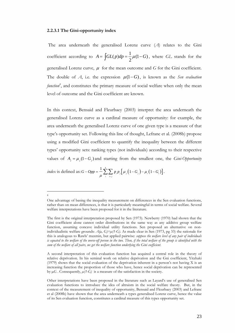
2.2.3.1 The Gini-opportunity index

The area underneath the generalised Lorenz curve (A) relates to the Gini

coefficient according to 1( ) (1 )2

A GL p dp Gµ= = −∫ , where GL stands for the

generalised Lorenz curve, µ for the mean outcome and G for the Gini coefficient.

The double of A, i.e. the expression (1 )Gµ − , is known as the Sen evaluation

function8, and constitutes the primary measure of social welfare when only the mean

level of outcome and the Gini coefficient are known.

In this context, Bensaid and Fleurbaey (2003) interpret the area underneath the

generalised Lorenz curve as a cardinal measure of opportunity: for example, the

area underneath the generalised Lorenz curve of one given type is a measure of that

type’s opportunity set. Following this line of thought, Lefranc et al. (2008b) propose

using a modified Gini coefficient to quantify the inequality between the different

types’ opportunity sets: ranking types (not individuals) according to their respective

values of (1 )j j jA Gµ= − and starting from the smallest one, the Gini-Opportunity

index is defined as: ( ) ( )[ ]11 1

k

i j j j i ii i j

G Opp p p G Gµ µµ <

− = − − −∑∑ .

8 One advantage of basing the inequality measurement on differences in the Sen evaluation functions, rather than on mean differences, is that it is particularly meaningful in terms of social welfare. Several welfare interpretations have been proposed for it in the literature. The first is the original interpretation proposed by Sen (1973). Newberry (1970) had shown that the Gini coefficient alone cannot order distributions in the same way as any additive group welfare function, assuming concave individual utility functions. Sen proposed an alternative on non-individualistic welfare grounds: A(µ, G)=µ(1-G). As made clear in Sen (1973, pg 33) the rationale for this is analogous to Rawls’ maxmin, but applied pairwise: suppose the welfare level of any pair of individuals is equated to the welfare of the worse-off person in the two. Then, if the total welfare of the group is identified with the sum of the welfare of all pairs, we get the welfare function underlying the Gini coefficient. A second interpretation of this evaluation function has acquired a central role in the theory of relative deprivation. In his seminal work on relative deprivation and the Gni coefficient, Yitzhaki (1979) shows that the social evaluation of the deprivation inherent in a person’s not having X is an increasing function the proportion of those who have, hence social deprivation can be represented by µG . Consequently, µ(1-G) is a measure of the satisfaction in the society. Other interpretations have been proposed in the literature such as Layard’s use of generalised Sen evaluation functions to introduce the idea of altruism in the social welfare theory. But, in the context of the measurement of inequality of opportunity, Bensaid and Fleurbaey (2003) and Lefranc et al (2008b) have shown that the area underneath a types generalised Lorenz curve, hence the value of its Sen evaluation function, constitutes a cardinal measure of this types opportunity set.

24

This index, gives the weighted average of the differences between the types’

opportunity sets in which the weights are the sample weights of the different types

( ),i jp . It increases in the number of types, therefore depending on the subjective

definition of these by the researcher9.

In the specific case of health, a potential limitation of this index concerns the fact

that the Gini coefficient, hence also the Gini-opportunity index, is not invariant to

the scale on which the health variable is measured. This is a well known fact, but the

use of mean based indices, such as Gini coefficients and concentration indices, as

well as of regression models that assume a particular scale of the health variable is

widespread: this is for example the approach used by Wagstaff et al. (1991),

Contoyannis et al. (2004) and Van Doorslaer and Koolman (2004) in the field of

health inequalities, and also the methodology implemented in many other papers

concerned with different aspects of health economics such as Case et al. (2005).

Resolving this limitation is therefore beyond the scope of this paper10. However, to

mitigate its impact and to ensure the robustness of the results, sensitivity analysis

was undertaken regarding the latent scale of the self-assessed health variable11.

2.2.3.2 An alternative approach

In some situations, the definition of social types has a clear intuitive appeal; in

others, however, it may be hard to justify. In order to avoid this downside, one may

treat each individual as a type: by assuming that the number of social types equals

the number of individuals, the Gini-opportunity index equals, by construction, the

conventional Gini coefficient.

9 The Gini-opportunity index also satisfies all the fundamental properties required by the indices of relative inequality: within type anonymity; between-type Pigou-Dalton principle of transfers; normalisation (if cdfs are equal, the index is equal to zero); homogeneity of degree zero; invariance to a replication of the population. For details see Lefranc et al. (2008b) and references therein. 10 A series of different possibilities to deal with this problem was recently proposed by Erreygers (2009). 11 A summary robustness check has been performed in order to assess the sensitivity of the inequality measures computed in the paper to different self-assessed health scales. This was carried-out using the McMaster Health Utility Index Mark III which is a truly cardinal health measure and has been used to cardinalise ordinal self-assessed health indices as shown in Van Doorslaer and Jones (2003). The McMaster Health Utility Index Mark III indicates lower and upper bounds for the health variable: in a five-point scale these are respectively [0; 0.428; 0 .756; 0.897; 0.947] and [0.428; 0.756; 0.897; 0.947; 1]. As a robustness check, the inequality measures computed in the chapter were recomputed using these alternative scales; the results were reassuring, showing that the reported measures are not significantly sensitive the use of these different health scales.

25

Fleurbaey and Schokkaert (2009) propose a range of different approaches to the

measurement of health inequalities that do not require the definition of a discrete

number of types. The measure used in this paper is inspired in one of them, the

conditional equality, and is computed as follows. After running i i ih Cα β ε= + + one

computes ˆ ˆ ˆβ ε= = −i i i ih C h . The pseudo-Gini coefficient12 is then applied directly

to ih , in order to measure the overall health inequality that is due to circumstances,

hence the extent of inequality of opportunity.

This approach diverges from Fleurbaey and Schokkaert (2009): the first stage

regression implemented in this paper omits all the effort variables; as pointed-out by

Gravelle (2003), this might lead to biased estimates, for the partial correlations

between circumstances and effort are not taken into account. However, in the

context of the Roemer model, these partial correlations should also be treated as

circumstances for they embody the indirect effect of the unjust circumstances on

health that is channelled through effort. This omission is therefore deliberate.

The value of this measure is directly comparable with that of the health pseudo-

Gini13 coefficient ( )iG h . The health pseudo-Gini coefficient has been used in the

literature to measure inequality of outcomes. It implicitly treats as circumstances all

the sources of variation in health and, therefore, the value of ( )iG h constitutes an

upper bound for inequality of opportunity. In turn, ( )iG h treats as circumstances

only the sources of unfair inequality that are labelled as such by the researcher; it is

therefore a lower bound for the extent of inequality of opportunity in health.

It is important to stress that these measures of inequality of opportunity are

inherently different and therefore do not necessarily bring about the same ranking

of social states. The Gini-opportunity index measures the inequality between a

discrete number of social types subjectively defined by the researcher. ( )iG h also

12 The outcome of interest in this paper is self-assessed health, measured in a discrete ordinal scale. Because of this, individuals cannot be simply ranked by health: grouped data is therefore used and pseudo-Lorenz curves and pseudo-Gini coefficients defined. 13 In this paper, ( )iG h denotes the pseudo-Gini coefficient.

26

requires a normative cut between circumstances and effort, but it respects the

continuous nature of these variables; it quantifies the overall contribution of

circumstances to the observed (health) outcome inequality. Finally, the pseudo-Gini

index is the standard tool for the measurement of pure health inequalities; it

implicitly assumes that all causes of inequality of opportunity are circumstances.

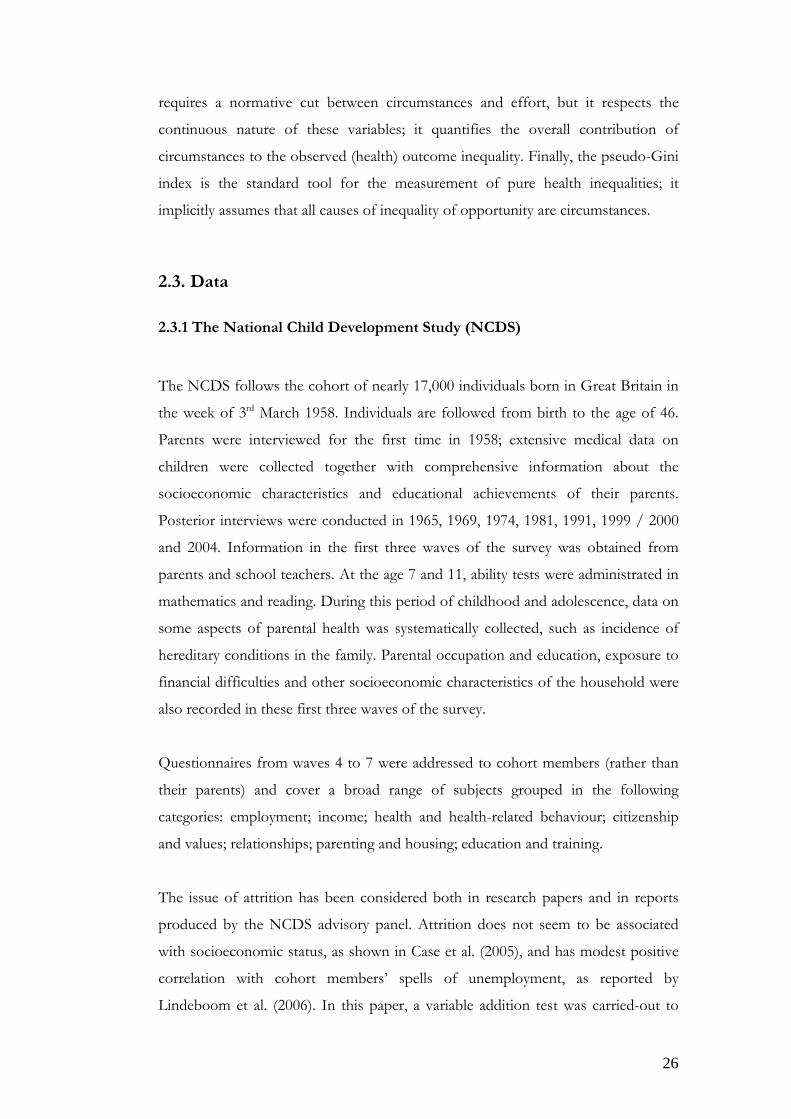
2.3. Data

2.3.1 The National Child Development Study (NCDS)

The NCDS follows the cohort of nearly 17,000 individuals born in Great Britain in

the week of 3rd March 1958. Individuals are followed from birth to the age of 46.

Parents were interviewed for the first time in 1958; extensive medical data on

children were collected together with comprehensive information about the

socioeconomic characteristics and educational achievements of their parents.

Posterior interviews were conducted in 1965, 1969, 1974, 1981, 1991, 1999 / 2000

and 2004. Information in the first three waves of the survey was obtained from

parents and school teachers. At the age 7 and 11, ability tests were administrated in

mathematics and reading. During this period of childhood and adolescence, data on

some aspects of parental health was systematically collected, such as incidence of

hereditary conditions in the family. Parental occupation and education, exposure to

financial difficulties and other socioeconomic characteristics of the household were

also recorded in these first three waves of the survey.

Questionnaires from waves 4 to 7 were addressed to cohort members (rather than

their parents) and cover a broad range of subjects grouped in the following

categories: employment; income; health and health-related behaviour; citizenship

and values; relationships; parenting and housing; education and training.

The issue of attrition has been considered both in research papers and in reports

produced by the NCDS advisory panel. Attrition does not seem to be associated

with socioeconomic status, as shown in Case et al. (2005), and has modest positive

correlation with cohort members’ spells of unemployment, as reported by

Lindeboom et al. (2006). In this paper, a variable addition test was carried-out to

27

investigate whether health-related attrition is a problem: ordered probit regressions

were used to determine whether being in subsequent waves of the panel is

correlated with health status. No evidence of health-related attrition was found.

2.3.2 Variables: health, circumstances and effort

The main health outcome considered in this paper is self-assessed health (SAH)

measured in a four-point scale: excellent, good, fair and poor health14. SAH is

measured when the cohort members are 23, 33, 42 and 46 years old. SAH is widely

used in health economics and was shown to predict mortality and deterioration of

health even after controlling for the medical assessment of health conditions: Idler

and Kasl (1995) provide an extensive literature review on this issue. In the specific

case of the NCDS, the focus on SAH is also corroborated by its high correlation

with reported disability and number of hospitalisations15.

Two sorts of circumstance variables are considered: the parental socioeconomic

background of the cohort members and their congenital and childhood health

conditions.

The socioeconomic background of the cohort members is characterised by a

comprehensive set of variables. The NCDS allows us to trace the social class of the

parents and of both grandfathers of the cohort members. This is derived from the

respective Registrar General’s Social Class in the first three waves of the survey (for

parents) and at the time in which parents left school (for the grandfathers).

Following the literature on the NCDS, data on wages were not taken directly into

account given substantial non-response. Along the lines of Case et al. (2005) and

Lindeboom et al. (2006), this was replaced by the incidence of financial difficulties

during the childhood of the cohort members. The number of years of schooling of

the mother and of the father is also included in the set of circumstances.

14 In the latest wave of the survey, SAH is however measured in a five-point scale which also includes the category of “very poor health”. 15 See Case et al. (2005, pp. 370).

28

The proxies for health endowment used in this paper have all been cited in the

literature as systematic determinants of adult health. Birthweight is taken as the

main indicator of health at birth; dummy variables for whether the mother smoked

after the fourth month of pregnancy and for whether the child was breastfed are

included as controls. The NCDS provides information about a comprehensive set

of morbidities experienced by the child up until the age of 16. Measures of

morbidity, which aggregate 12 categories of health conditions, are constructed

according to Power and Peckham (1987) and treated as circumstances. Dummy

variables for the occurrence of chronic diseases in the parents and for the incidence

of hereditary conditions such as diabetes and epilepsy in parents, brothers and

sisters of the cohort members complement the information on health endowments.

Dummy variables for whether the child was obese at age 16 and for whether both

parents were smokers in 1974 are also treated as circumstances.

The effort factors considered in the paper are health-related lifestyles such as

cigarette smoking, alcohol consumption, consumption of fried food and educational

attainment: these are strongly constrained by circumstances, but also reflect

individual choices.

All the variables used to proxy lifestyles are based on self-reported information. The

variable for cigarette smoking is the self-reported number of cigarettes smoked per

day. Alcohol consumption is measured by the number of units of alcohol consumed

on average per week: NCDS respondents are asked about their weekly consumption

of a wide range of alcoholic drinks (glasses of wine, pints of beer and so forth).

These were then converted to units of alcohol using the UK National Health

Service official guidelines16. Educational attainment is measured by the highest

academic qualification awarded to cohort members17. The summary statistics of the

main variables used in the paper is shown in Table 1.

16 These are publicly available at: http://www.nhsdirect.nhs.uk/magazine/interactive/drinking/index.aspx . 17 O-level (Ordinary levels) were a secondary education qualification corresponding, typically, to 11 years of education; A-levels (Advanced levels) are a qualification which corresponds to 13 years of education. Completion of A-levels is a prerequisite for university admission.

29

2.4 Testing and measuring inequality of opportunity in health

The existence of inequality of opportunity in health can be tested using the set of

conditions defined in Section 2.2.2. As explained above, the data are consistent with

inequality of opportunity if ( ) ( )', | | ' .FSDC C F H C F H C∀ ≠ In order to

illustrate the application of this condition to the NCDS data, three social types are

defined on the sole basis of the social class of the cohort members’ father in 1974: a

top class including professional and managerial workers, a middle class including

partially skilled non-manual and skilled manual workers, and a bottom class

including unskilled manual and unemployed workers.

The outcome of interest is self-assessed health at age 46, measured in a five-point

scale. Given the existence of a common discrete support, Kolmogorov-Smirnov

test procedures were carried-out to test for first degree stochastic dominance

between types; this approach was previously used in the literature by Lefranc et al.

(2004) and Devaux et al. (2008). Table 2 shows the results of these tests: the

distribution of health in the top social class dominates at first degree that of the

middle class which, in turn, dominates, also at first degree, the outcome distribution

of the bottom social type at the 5% significance level. These results establish the

existence of inequality of opportunity between types.

Two approaches to the measurement of inequality of opportunity were presented in

Section 2.2.3. The first of them, the Gini-opportunity index, is implemented using

the social types defined for testing for stochastic dominance, and its values

tabulated for the four latest waves of the NCDS in the first column of Table 3. This

index measures the extent of inequality of opportunity between the three social

types when the cohort members were 23, 33, 42 and 46 years old. To allow for

sampling error, the standard errors of the Gini-opportunity indices are

bootstrapped in each wave, with independent re-sampling within each of the three

types.

30

The second column of Table 3 presents the values of the pseudo-Gini coefficient

( )iG h , which measures the overall inequality that is attributable to circumstances,

avoiding the subjective definition of social types. It is computed as described in

Section 2.2.3. The circumstances used in the regression are the following18: gender,

regional dummies, socioeconomic status of the father and of both grandfathers,

number of years of education of the father and of the mother, indicators for

whether the father and the mother were smokers in 1974, birthweight, incidence of

physical and mental impairments during childhood and adolescence, exposure to

financial hardship at age 11 and at age 16, indicators for the prevalence of diabetes,

epilepsy and other (unspecified) chronic conditions in the family and a dummy

variable for whether the cohort member was obese at age 16. This equation is the

same for all the waves, making the values of ( )iG h directly comparable.

The third column of Table 3 displays the values of the health pseudo-Gini

coefficient ( )iG h . As seen in Section 2.2.3, this measure treats all the sources of

variation in health as circumstances, equating inequality of opportunity and

inequality of outcomes; ( )iG h is therefore an upper bound to the extent of

inequality of opportunity.

The Gini-opportunity index, exhibits a remarkable persistence over the time: it does

not change significantly over the last three waves of the survey. This suggests that

the long term association between parental socioeconomic status and the cohort

members’ health is far from being restricted to childhood and adolescence. The

values of ( )iG h and ( )iG h show an increasing trend, as the 1958 cohort ages and

the prevalence of illness mounts19.

18 As explained above, this procedure is in line with van Doorslaer et al. (2004), in the sense that only circumstance variables are used in the first stage regression. 19 It must be stressed that there is no theoretical reason ensuring that the three indices depict the same trend. For example, Lefranc et al. (2008b: p.539-540) use a dataset of 9 countries to compare the extent of income inequality (measured by the Gini coefficient) with that of the inequality of opportunity for the acquisition of income (measured by the Gini-opportunity index). Their results show that the correlation between the values of these two measures can be negative in practice.

31

The fourth column of Table 3 displays the ratio ( )iG h / ( )iG h ; this corresponds

to the proportion of total health inequality that is due to inequality of opportunity

(i.e. due to the direct and indirect effect of the observed circumstances). The

weight of inequality of opportunity in the total health inequality is relatively steady

across the four waves, assuming values between 21% and 26%. Since these

circumstances affect the cohort members before age 16, at least 21% of the health

inequalities observed in adulthood are due to factors which are only amenable to

policy interventions early in life.

2.5 Estimation results

So far the analysis has been focused on identifying and measuring inequality of

opportunity in health. The attention is now turned to explaining it. On a first stage,

a model of association between self-assessed health (SAH) at age 46 and a

comprehensive set of circumstances is estimated; this allows an assessment of the

global impact of circumstances on health. These estimates are then contrasted with

those of an alternative model, which controls for effort variables; this compares the

relative importance of the pathway of circumstance through effort, with its direct

effect. The estimates of the effort factors must however be seen as associations that do

not necessarily reflect causality. Finally, in order to illuminate further the triangular

relationship between circumstances, effort and health, a set of univariate equations is

estimated for each of the effort variables.

2.5.1 Adult health and early life circumstances: direct and indirect effects

Table 4 shows the results of the ordered probit regression of SAH at age 46 on

circumstances. A general-to-simple kitchen sink approach was followed, starting with

a large number of regressors, all of them potential circumstances. These

circumstance variables are also the ones used to compute ( )iG h in Table 3. The

reported marginal effects are computed by averaging across all the individual

marginal effects in the sample, and by taking excellent health as the reference category.

32

The estimated coefficients for the social class of the cohort member’s father are

positive and statistically significant. Compared with the bottom social class,

individuals whose father or male head of household is in the top occupational

category are 5.7 percentage points more likely to report excellent health. This partial

effect is of 4.1 percentage points for the middle social class. These facts are striking

given the large number of controls used and mirror the results of the stochastic

dominance analysis, confirming the existence of inequality of opportunity in health.

The number of years of education of the mother is significantly associated with

good health in adulthood; paternal education is however statistically insignificant

after controlling for paternal social class. This is in line with Case et al. (2005, pp

377); it is also a statistically significant result for women, but not for men.

Financial difficulties at age 16, are a statistically significant determinant of health

deterioration in adulthood, especially for men: spells of bad household finances at

age 16 are associated with a 13.4 percentage points lower probability of reporting

excellent health at age 46. Propper et al. (2004) show that spells of low income in

early years affect health in childhood and adolescence; the results in Table 4 make

clear that this association persists in adulthood.

Health endowments are also crucial: the incidence of illness in adolescence is

significantly correlated with a worsening of self-reported health at age 46. Marginal

effects are identical for men and women, corresponding to a nearly 2 percentage

points lower probability of reporting excellent health. The prevalence of obesity at

age 16 is also highly correlated with a deterioration of adult health. This effect is

statistically significant for women (but not for men) and accounts for a reduction of

around 8.4% in the probability of reporting excellent health in adulthood.

Table 4 accounts for the global impact of circumstances on SAH at age 46, but it

omits important determinants of health, namely effort factors. These are added to

the model in Table 5.

After controlling for many of the factors that individuals partially control, and

including among them educational attainment and even own social class at age 33,

most of the circumstances preserve their statistical significance. However, the size

33

of the marginal effects20 of circumstances such as parental social class and bad

finances at age 16 are strongly reduced. This indicates that only a fraction of the

effect of circumstances is a direct one: effort factors now capture part of their

impact on health.

The health endowment circumstances that were statistically significant in Table 4

remain significant in Table 5; their marginal effects are also reduced. Particularly

striking is the fact that obesity at age 16 remains statistically significant after

controlling for a series of lifestyles and dietary choices, carrying a negative partial

effect of nearly 4 percentage points. Although this is statistically significant only for

women, it suggests that childhood obesity has an important direct effect on adult

health, therefore amenable only to early policy interventions.

Amongst effort factors, the detrimental effect of cigarette smoking on SAH is

prominent. This is in line with most of the literature: Power and Peckham (1987),

Marmot et al. (2001), Contoyannis and Jones (2004) and Balia and Jones (2008)

report similar results. The avoidance of fried food is the only dietary choice that

shows a statistically significant positive impact on SAH at age 46.

After controlling for own social class in adulthood and for a commonly used proxy

of intellectual ability (maths test scores at age 11), the attainment of A-levels or

higher academic qualifications shows to be statistically significant: compared with

those with no secondary education, individuals attaining at least A-levels have an

approximately 1.3 percentage points higher probability of reporting excellent

health21. Finally, the effect of (own) social class is also statistically significant:

compared to the bottom social category, individuals in the top and middle classes

have a nearly 1.5 percentage points higher probability of reporting excellent health

at age 46. However, it must be noted that these results encase important gender

differences. The association between academic qualifications and self-assessed

health at age 46 is sizable and statistically significant for men, but not for women.

Also, the estimated marginal effect of own social class in adulthood is substantial

20 The marginal effects in Table 5 are also for the probability of reporting excellent health. 21 This makes clear that there is an association between educational attainment and self-assessed health at age 46 over and above the effect of professional occupation in adulthood. This would not occur if education were a pure job marketing signalling device.

34

for men but practically null for women. This is consistent with the existence of

marked differences in labour market opportunities between male and female

cohort-members, which may partly explain the observed gender-asymmetric health

returns by educational qualifications.

2.5.2 Circumstances and effort: primary pathways

In order to illuminate further the effect of circumstances on effort, single equations for

each of the most important effort variables are estimated in Table 6.

The first and second equations of the table concern cigarette smoking. The number

of cigarettes smoked per day shows a spike at zero, which is typical of cigarette

smoking data. In order to take this into account, two equations are estimated: the

first is a probit model, estimated for the whole sample, for whether an individual is

a smoker or a non-smoker; the second, features the logarithm of the number of

cigarettes smoked as the dependent variable and is estimated only for smokers.

Parental smoking, bad household finances at age 16 and the prevalence of

hereditary conditions in the family are chief determinants of cigarette smoking at

age 33. Parental smoking accounts for a statistically significant increase in the

probability of smoking of 3.6 percentage points, in the case of the father, and of

around 2.4 percentage points in the case of the mother. The partial effect of

financial difficulties in adolescence is even larger: 9.2 percentage points. Conversely,

the prevalence of chronic diseases in the family, other than diabetes and epilepsy,

has a statistically significant negative partial effect of 9.8 percentage points. This

corroborates the thesis that perceived physical frailty leads to the adoption of

healthy lifestyles to offset health risks.

Finally, the results suggest the existence of a socioeconomic and educational

gradient in the probability of smoking: those with higher qualifications are less likely

to smoke, even after controlling for own and parental socioeconomic status.

Although the estimates of academic qualifications should not be seen as causal

effects, this backs the idea that complementary educational policies may be crucial

to reduce inequality of opportunity in health.

35

The evidence concerning the number of cigarettes smoked per day is mixed: there is

neither a clear socioeconomic gradient nor an educational gradient. This is in accord

with papers such as Jones (1989): education and social status reduce the probability

of an individual becoming a smoker; however, for those who are already smokers,

tobacco is a normal good.

The third equation in Table 6 is an ordered probit with degrees of avoidance of

fried food as the dependent variable. The results suggest that males are less likely to

avoid fried food than females. Those hit by financial hardship at age 16 are

approximately 6.3 percentage points less likely to be in the highest category of fried

food avoidance. Education matters once more: individuals reporting at least O-

levels bear a positive and statistically significant association with the avoidance of

fried food. Of special interest, however, is the positive and statistically significant

effect of obesity at age 16; this corresponds to an estimated partial effect of

approximately 7 percentage points. This is once again in line with the rationale of

risk offsetting in face of perceived frailty, and confirms that the harmful impact of

child obesity on adult health is largely a direct one that needs to be tackled early in

life.

Given the substantial influence of education on other effort variables and on health,

a final note concerns the estimates of the impact of circumstances on the

probability of attaining each educational level. The last three columns of Table 6

give probit estimates for three levels of education: academic degree or equivalent,

A-levels or higher and O-levels or higher.

Women are more likely to report having at least O-levels; however, men are more

likely to attain a university degree. Ill health in childhood and obesity at age 16,

bear a negative but statistically insignificant association with the educational

outcomes. These are largely sensitive to the social position of the parents: parental

education has a positive and statistically significant impact on all levels of

educational attainment and bad finances at age 16 accounts for a statistically

significant reduction of roughly 4.6 percentage points of the probability of reporting

O-levels or a higher qualification. This suggests that equality of opportunity in

education may a key factor to reduce inequality of opportunity in health,

36

highlighting the potential for complementary policies between the educational and

health care sectors.

2.6 Conclusions

This paper proposes two approaches to measuring inequality of opportunity in

heath and finds evidence of such inequality among NCDS cohort members. The

results suggest that at least 21% of the health inequalities observed in adulthood are

due to inequality of opportunity.

Econometric models are used to identify the most influential circumstances beyond

individual control and to quantify their impact. Accounting for a comprehensive set

of controls, parental socioeconomic status is a crucial explanatory factor of self

assessed health in adulthood. The education of the mother (but not of the father) is

also crucial, but mostly for women. Spells of financial difficulties during childhood

and adolescence are particularly detrimental to men: alone, these are associated to a

13.4 percentage points reduction in the probability of reporting excellent health at

age 46. In terms of health endowments, ill health during childhood is negatively

associated with SAH at age 46, affecting both men and women. Obesity in

childhood and adolescence is negatively associated with health at age 46, and is

mainly detrimental to women.

Once effort factors, such as lifestyles and educational attainment, are added to the

model, most of the circumstances remain statistically significant, although their

marginal effects are reduced. This suggests that, although part of their effect is

channelled through effort, an important part of it is a direct one.

Separate equations are estimated for each of the effort factors, to illuminate the

indirect pathways of the effect of circumstances through effort. The results show

that the influence of circumstances on effort factors can be paramount, as for

example in the cases of cigarette smoking and educational attainment. They also

suggest that inequality of opportunity in the educational sector may exacerbate

health inequalities via the influence that education exerts on lifestyles.

37

Policy implications are inferred. Some unjust circumstances are only amenable to

policy during childhood. Moreover, given that parental characteristics are among

the most influential circumstances, policy interventions aimed at young adults, and

namely at young parents, may be crucial to prevent inequality of opportunity from

carrying over from one generation to the next. Finally, since the influence of

circumstances on health is often channelled through effort, key complementary

policies to reduce health inequalities may need to be implemented outside the health

care system and, in particular, in the educational sector.

38

Appendix A Table 1: Summary statistics

Variable Mean Std. Dev. Min MaxSelf-assessed health, age 46 3.987719 0.9302554 1 5Male 0.5171652 0.4997187 0 1Parental socioeconomic status at birth: high 0.2727015 0.4453612 0 1Parental socioeconomic status at birth: middle 0.49983 0.5000141 0 1Paternal grandfather's socioeconomic status 1.975576 0.7470104 1 3Maternal grandfather's socioeconomic status 2.04248 0.7366398 1 3Years of education: father 9.904075 1.621967 7 16Years of education: mother 9.916638 1.376012 7 16Indicator: mother smoker, age 16 0.7865378 1.010508 0 4Indicator: father smoker, age 16 1.119048 1.136957 0 4Indicator: maternal smoking after 4th month of pregnancy 0.3364165 0.472497 0 1Indicator: breastfead 0.6421394 0.4793864 0 1Birthweight 128.3177 72.43585 11 509Physical / mental impairments, age 16 2.236591 1.541278 0 10Indicator: financial hardship, age 11 0.0714425 0.2575708 0 1Indicator: financial hardship, age 16 0.0789546 0.269677 0 1Indicator: diabetes in parents, brothers or sisters 0.0212642 0.1442684 0 1Indicator: epilepsy in parents, brothers or sisters 0.073906 0.2616263 0 1Indicator: other hereditary chronic condition 0.025154 0.1565977 0 1Indicator: chronic conditions in cohort member's mother, age 16 0.0477003 0.2131386 0 1Indicator: obesity, age 16 0.0324388 0.1771673 0 1Indicator: university degree or equivalent 0.2313824 0.4217384 0 1Indicator: A-levels or higher qualification 0.3206419 0.4667478 0 1Indicator: O-levels, or higher qualification 0.8212712 0.3831451 0 1Mathematics test score, age 11 (scores range from 0 to 40) 15.23885 11.01308 0 40Indicator : smoker, age 33 0.3197992 0.4664195 0 1Number of cigarettes per day 5.543246 9.519264 0 70Arguments with parents about risks of smoking 0.0913892 0.2881695 0 1Avoidance of fried food in diet: weekly frequency (1 to 6), age 33 4.538137 0.9861445 1 6Weekly consumption of vegetables, age 33 0.6580174 0.638489 0 2Weekly alcohol consumption, age 33 2.453389 1.619937 0 4Sweets consumption: weekly frequency, age33 4.152178 1.667634 1 9Socioeconomic status: high (age 33) 0.5977131 0.4903824 0 1Socioeconomic status: middle (age 33) 0.2081837 0.4060281 0 1

Full sample

39

Table 2: Tests for stochastic dominance between types

Null hypothesis Corrected P valueNull: Type 1 FSD type 2 0.999Null: Type 1 FSD type 3 0.999Null: Type 2 FSD type 3 0.959

Figure 1: SAH (age 46) by parental socioeconomic group

40

Table 3: Measures of inequality of opportunity

Wave 4: 1981 (age 23) 0.0088496 0.02205 0.10257 0.21497

(0.0017707)Wave 5: 1991 (age 33) 0.0165535 0.02976 0.11304 0.26326

(0.0015658)Wave 6: 1999/2000 (age 42) 0.018381 0.03257 0.12765 0.25515

(0.0018364)Wave 7: 2004 (age 46) 0.0178522 0.0338 0.15405 0.2194

(0.0026443)Note: Bootstrapped standard errors in parentheses, with independent re-sampling within each of the three types.

Ratio: Health Pseudo-Gini:NCDS wave Gini-opportunity index ( )iG h ( )iG h( )( )

i

i

G h

G h

41

Table 4: Adult health and circumstances*. Ordered probit estimates

Dependent variable:Self-assessed health (age 46) Coefficient Marginal Eff.† Coefficient Marginal Eff.† Coefficient Marginal Eff.†

Parental SES at birth: High 0.202*** 0.0574 0.239*** 0.0401 0.163* 0.0616(0.0615) (0.0855) (0.0897)

Parental SES at birth: Middle 0.142*** 0.0414 0.185*** 0.0330 0.104 0.0394(0.0459) (0.0633) (0.0676)

Paternal grandfather SES -0.0287 -0.00836 -0.0374 -0.00665 -0.0137 -0.00520(0.0293) (0.0409) (0.0424)

Maternal grandfather SES -0.0171 -0.00498 0.00123 0.000220 -0.0392 -0.0149(0.0247) (0.0345) (0.0356)

Years of education: Father -0.0116 -0.00338 -0.00838 -0.00149 -0.0185 -0.00704(0.0130) (0.0184) (0.0186)

Years of education: Mother 0.0282* 0.00823 0.0378* 0.00672 0.0183 0.00697(0.0148) (0.0203) (0.0218)

Mother smoker (age 16) -0.0491** -0.0143 -0.0489 -0.00871 -0.0439 -0.0167(0.0221) (0.0307) (0.0321)

Father smoker (age 16) -0.0158 -0.00462 -0.0228 -0.00405 -0.0144 -0.00548(0.0158) (0.0218) (0.0230)

Maternal smoking during pregnancy 0.0132 0.00384 0.0229 0.00406 -0.00707 -0.00269(0.0450) (0.0622) (0.0656)

Breastfed 0.0541 0.0159 0.0845 0.0154 0.0181 0.00688(0.0371) (0.0523) (0.0529)

Birthweight 0.000377 0.000110 0.000987** 0.000176 -0.000115 -4.37e-05(0.000258) (0.000400) (0.000342)

Mathematics test score: age 11 0.00455*** 0.00133 0.00475** 0.000846 0.00468** 0.00178(0.00164) (0.00237) (0.00231)

Physical / mental impairments (age 16) -0.0760*** -0.0222 -0.0846*** -0.0151 -0.0647*** -0.0246(0.0109) (0.0150) (0.0162)

Financial hardship (age 11) -0.0653 -0.0195 -0.216** -0.0431 0.134 0.0502(0.0802) (0.110) (0.119)

Financial hardship (age 16) -0.201** -0.0627 -0.0825 -0.0153 -0.346*** -0.134(0.0791) (0.113) (0.112)

Diabetes in parents or siblings -0.0680 -0.0203 0.160 0.0260 -0.353** -0.137(0.110) (0.149) (0.164)

Epilepsy in parents or siblings -0.0856 -0.0256 0.00330 0.000587 -0.178* -0.0685(0.0640) (0.0910)

Other hereditary chronic condition -0.0685 -0.0205 -0.0483 -0.00884 -0.0566 -0.0216(0.107) (0.152) (0.152)

Chronic condition: Mother (age 16) -0.0880 -0.0264 -0.114 -0.0215 -0.0619 -0.0237(0.0801) (0.113) (0.115)

Obesity (age 16) -0.268*** -0.0848 -0.341*** -0.0724 -0.173 -0.0668(0.0788) (0.108) (0.116)

Number of observations 4408 2220 2188

Notes: Standard errors in parentheses; *** p<0.01, ** p<0.05, * p<0.1Coefficients and marginal effects for regional variables are suppressed here (due to statistical insignifiance) but available upon request.*The same circumstances used to compute in Table 3.† Marginal effects for the probability of reporting excellent health .

Full sample Women Men

( )iG h

42

Table 5: Adult health, circumstances and effortOrdered probit estimatesDep. Variable:SAH (age 46) Coefficient Marginal Eff.* Coefficient Marginal Eff.* Coefficient Marginal Eff.*

Circumstance variablesParental SES at birth: High 0.222*** 0.0274 0.315*** 0.00922 0.126 0.0336

(0.0696) (0.0957) (0.103)Parental SES at birth: Middle 0.104** 0.0137 0.150** 0.00518 0.0571 0.0154

(0.0523) (0.0711) (0.0780)Paternal grandfather SES 0.0178 0.00233 0.0282 0.000958 0.0220 0.00595

(0.0333) (0.0458) (0.0491)Maternal grandfather SES -0.0123 -0.00161 0.0106 0.000359 -0.0463 -0.0125

(0.0278) (0.0383) (0.0411)Years of education: Father -0.00986 -0.00129 -0.0214 -0.000727 0.000520 0.000140

(0.0144) (0.0203) (0.0207)Years of education: Mother 0.0254 0.00332 0.0438* 0.00149 0.00861 0.00233

(0.0166) (0.0229) (0.0245)Mother smoker (age 16) -0.0432* -0.00567 -0.0605* -0.00206 -0.0183 -0.00493

(0.0253) (0.0346) (0.0379)Father smoker (age 16) -0.00738 -0.000967 -0.0250 -0.000847 0.00699 0.00189

(0.0179) (0.0246) (0.0265)Maternal smoking during pregnancy 0.0355 0.00461 0.0808 0.00268 -0.0379 -0.0103

(0.0512) (0.0700) (0.0765)Breastfed 0.0630 0.00841 0.0833 0.00291 0.0542 0.0148

(0.0420) (0.0585) (0.0611)Birthweight 0.000645** 8.45e-05 0.000773* 2.62e-05 0.000430 0.000116

(0.000308) (0.000450) (0.000428)Physical / mental impairments (age 16) -0.0733*** -0.00962 -0.0660*** -0.00224 -0.0827*** -0.0223

(0.0123) (0.0169) (0.0185)Financial hardship (age 11) -0.0350 -0.00469 -0.185 -0.00742 0.185 0.0465

(0.0923) (0.124) (0.140)Financial hardship (age 16) -0.156* -0.0225 -0.0624 -0.00224 -0.292** -0.0870

(0.0911) (0.129) (0.131)Diabetes in parents or siblings -0.0832 -0.0115 0.108 0.00330 -0.341* -0.103

(0.123) (0.166) (0.187)Epilepsy in parents or siblings -0.0651 -0.00886 -0.0436 -0.00154 -0.105 -0.0293

(0.0741) (0.103) (0.109)Other hereditary chronic condition -0.103 -0.0144 -0.0377 -0.00133 -0.142 -0.0402

(0.122) (0.170) (0.179)Chronic condition: Mother (age 16) -0.130 -0.0185 -0.135 -0.00516 -0.142 -0.0402

(0.0942) (0.129) (0.141)Mathematics test score: age 11 0.000855 0.000112 0.000727 2.46e-05 0.00133 0.000359

(0.00203) (0.00283) (0.00295)Obesity (age 16) -0.268*** -0.0414 -0.393*** -0.0190 -0.119 -0.0336

(0.0877) (0.119) (0.132)Effort variablesUniversity degree or equivalent -0.0619 -0.00832 -0.0361 -0.00126 -0.126 -0.0347

(0.0700) (0.0948) (0.105)A-levels or higher qualification 0.104* 0.0132 0.0421 0.00140 0.192* 0.0508

(0.1102) (0.0892) (0.103)O-levels or higher qualification 0.0452 0.00606 0.141 0.00530 -0.0249 -0.00667

(0.0631) (0.0924) (0.0876)Indicator(smoker)*Log(cigarettes/day)† -0.124*** -0.0163 -0.104*** -0.00352 -0.145*** -0.0392

(0.0159) (0.0224) (0.0231)Fried food avoidance: frequency† 0.0549*** 0.00720 0.0782** 0.00266 0.0425 0.0115

(0.0206) (0.0311) (0.0291)Weekly vegetables consumption† -0.0224 -0.00293 -0.0476 -0.00162 0.0340 0.00917

(0.0302) (0.0411) (0.0463)Weekly alcohol consumption† 0.00296 0.000388 0.00127 4.30e-05 -0.00881 -0.00238

(0.0145) (0.0239) (0.0200)Sweets consumption: frequency† 0.00347 0.000455 0.00118 4.00e-05 0.00480 0.00130

(0.0117) (0.0161) (0.0172)Own socioeconomic status: High† 0.111** 0.0149 0.110 0.00385 0.0964 0.0262

(0.0550) (0.0685) (0.0945)Own socioeconomic status: Middle† 0.128** 0.0159 0.0984 0.00307 0.115 0.0305

(0.0633) (0.112) (0.0919)

Number of observations 3535 1833 1702

Notes: Standard errors in parentheses; *** p<0.01, ** p<0.05, * p<0.1Coefficients and marginal effects for regional variables are suppressed here (due to statistical insignifiance) but available upon request.*Marginal effects for the probability of reporting excellent health .† denotes 'at age 33'.

Full sample Women Men

43

Table 6: The impact of circumstances on effort

Coefficient Marg. Eff. Coefficient Marg. Eff. Coefficient Marg. Eff. Coefficient Marg. Eff. Coefficient Marg. Eff. Coefficient Marg. Eff.Male -0.0326 -0.0101 0.0655 0.0655 -0.573*** -0.222 0.0859* 0.0214 0.0399 0.0107 -0.179*** -0.0283

(0.0492) (0.0475) (0.0381) (0.0517) (0.0505) (0.0660)Parental SES at birth: High -0.0878 -0.0269 -0.0324 -0.0324 -0.0459 -0.0171 0.0507 0.0127 0.0965 0.0262 -0.0366 -0.00581

(0.0852) (0.0792) (0.0665) (0.0976) (0.0931) (0.111)Parental SES at birth: Middle -0.0384 -0.0119 -0.0521 -0.0521 -0.0320 -0.0120 0.0152 0.00377 0.0633 0.0169 0.0473 0.00747

(0.0637) (0.0581) (0.0504) (0.0780) (0.0735) (0.0772)Paternal grandfather SES -0.0278 -0.00858 0.0696* 0.0696 -0.0523* -0.0196 -0.0887* -0.0220 -0.119*** -0.0317 -0.0936* -0.0148

(0.0411) (0.0395) (0.0317) (0.0457) (0.0435) (0.0536)Maternal grandfather SES 0.0276 0.00853 0.0131 0.0131 -0.0217 -0.00811 0.000487 0.000121 -0.0121 -0.00323 0.0136 0.00214

(0.0344) (0.0331) (0.0263) (0.0374) (0.0361) (0.0451)Years of education: Father 0.0323* 0.00999 -0.0107 -0.0107 -0.00219 -0.000818 0.0435** 0.0108 0.0487*** 0.0130 0.0195 0.00308

(0.0180) (0.0167) (0.0137) (0.0176) (0.0181) (0.0294)Years of education: Mother 0.0597*** 0.0184 -0.0164 -0.0164 -0.0375** -0.0140 0.131*** 0.0326 0.164*** 0.0438 0.101*** 0.0159

(0.0206) (0.0195) (0.0157) (0.0201) (0.0209) (0.0343)Mother smoker (age 16) 0.0791*** 0.0244 0.0372 0.0372 -0.0222 -0.00832 0.00256 0.000636 -0.0414 -0.0111 -0.0782** -0.0123

(0.0303) (0.0268) (0.0241) (0.0350) (0.0339) (0.0382)Father smoker (age 16) 0.120*** 0.0369 0.0571*** 0.0571 -0.00447 -0.00167 -0.0493** -0.0122 -0.0633*** -0.0169 -0.0920*** -0.0145

(0.0216) (0.0198) (0.0170) (0.0247) (0.0236) (0.0276)Maternal smoking during pregnancy -0.0586 -0.0179 0.0810 0.0810 0.0491 0.0183 0.00978 0.00244 -0.0253 -0.00677 -0.00255 -0.000402

(0.0622) (0.0569) (0.0486) (0.0705) (0.0683) (0.0793)Breastfed 0.00416 0.00128 -0.00747 -0.00747 -0.000747 -0.000279 0.0391 0.00969 -0.0266 -0.00712 0.0260 0.00412

(0.0517) (0.0488) (0.0398) (0.0576) (0.0553) (0.0664)Birthweight -0.000152 -4.70e-05 0.000313 0.000313 0.000367 0.000137 -0.000178 -4.43e-05 0.000250 6.70e-05 0.00117* 0.000184

(0.000367) (0.000362) (0.000280) (0.000405) (0.000389) (0.000545)Physical/mental impairments (age 16) 0.00579 0.00179 0.00740 0.00740 0.00202 0.000756 -0.0114 -0.00283 -0.00889 -0.00238 0.00696 0.00110

(0.0152) (0.0143) (0.0117) (0.0167) (0.0162) (0.0200)Financial hardship (age 11) 0.280*** 0.0925 0.0913 0.0913 -0.171** -0.0637 -0.0267 -0.00660 -0.0734 -0.0195 -0.262** -0.0461

(0.106) (0.0855) (0.0868) (0.150) (0.141) (0.120)Financial hardship (age 16) 0.100 0.0318 -0.141 -0.141 0.0286 0.0107 -0.173 -0.0411 -0.112 -0.0295 -0.350*** -0.0638

(0.110) (0.0905) (0.0888) (0.162) (0.148) (0.119)Diabetes in parents or siblings 0.0747 0.0235 0.0929 0.0929 -0.00731 -0.00273 0.116 0.0297 0.0756 0.0204 -0.0461 -0.00741

(0.155) (0.143) (0.121) (0.170) (0.168) (0.201)Epilepsy in parents or siblings 0.00600 0.00186 -0.0762 -0.0762 -0.0103 -0.00386 -0.0412 -0.0102 0.120 0.0327 0.243 0.0345

(0.0905) (0.0838) (0.0703) (0.105) (0.0980) (0.122)Other hereditary chronic condition -0.358** -0.0989 0.0540 0.0540 -0.0429 -0.0160 -0.224 -0.0524 -0.264 -0.0680 -0.0146 -0.00231

(0.163) (0.169) (0.117) (0.188) (0.179) (0.189)Chronic condition: Mother (age 16) -0.0866 -0.0261 -0.0388 -0.0388 -0.0584 -0.0218 0.105 0.0267 0.126 0.0341 -0.0403 -0.00646

(0.119) (0.113) (0.0903) (0.129) (0.126) (0.146)Obesity (age 16) -0.120 -0.0360 0.0525 0.0525 0.188** 0.0697 -0.157 -0.0374 -0.0570 -0.0151 0.00271 0.000427

(0.110) (0.108) (0.0851) (0.130) (0.121) (0.135)Mathematics test score: age 11 -0.00341 -0.00105 -0.000888 -0.000888 -0.00108 -0.000403 0.0317*** 0.00789 0.0409*** 0.0109 0.0358*** 0.00564

(0.00251) (0.00247) (0.00191) (0.00255) (0.00248) (0.00339)University degree or equivalent -0.189** -0.0570 -0.151 -0.151 0.0853 0.0319 ______ ______ ______ ______ ______ ______

(0.0910) (0.0980) (0.0659) ______ ______ ______ ______ ______ ______A-levels or higher qualification -0.192** -0.0586 -0.101 -0.101 0.0868 0.0325 ______ ______ ______ ______ ______ ______

(0.0848) (0.0882) (0.0633) ______ ______ ______ ______ ______ ______O-levels or higher qualification -0.377*** -0.127 0.0167 0.0167 0.186*** 0.0698 ______ ______ ______ ______ ______ ______

(0.0728) (0.0611) (0.0598) ______ ______ ______ ______ ______ ______Own socioeconomic status: High† -0.234*** -0.0746 -0.108* -0.108 0.107** 0.0403 0.634*** 0.150 0.737*** 0.201 0.648*** 0.110

(0.0656) (0.0596) (0.0527) (0.0854) (0.0781) (0.0766)Own socioeconomic status: Middle† -0.0302 -0.00927 -0.0214 -0.0214 -0.129** -0.0486 -0.223* -0.0534 -0.213** -0.0566 0.270*** 0.0398

(0.0767) (0.0673) (0.0617) (0.114) (0.103) (0.0873)Constant -1.025*** 2.674*** -3.520*** -3.629*** -0.462

(0.296) (0.290) (0.312) (0.315) (0.441)

Number of observations 3660 994 3727 3738 3738 3738

Notes: Standard errors in parentheses; *** p<0.01, ** p<0.05, * p<0.1. Coefficients and marginal effects for regional variables are suppressed here (due to statistical insignifiance) but available upon request.† at age 33.‡ or equivalent.

(Probit estimates)A-levels or higherUniversity degree‡

(Probit estimates) (OLS estimates) (Ordered probit estimates) (Probit estimates) (Probit estimates)O-levels or higher

Dep. Variable Dep. VariableIndicator: Smoker Cigarettes / day Fried food

Dep. Variable Dep. Variable Dep. Variable Dep. Variable

Chapter 3

Modelling Opportunity in Health under Partial Observability of Circumstances

3.1 Introduction Recent empirical papers, such as Trannoy et al. (2009) and Rosa Dias (2009),

provide evidence of substantial and persistent inequality of opportunity in health in

European countries. They also suggest that unjust circumstances affect health

through a network of indirect effects whose causal nexus is often ambiguous. This

has lead authors such as Fleurbaey and Schokkaert (2009) to propose that such

complex interactions be clarified through the specification of a structural model of

unfair inequalities; this paper follows this line of research.

This paper is grounded on the framework of Roemer (1998, 2002), which draws a

distinction between circumstance and effort variables: the outcome of interest is health as an

adult; circumstances (beyond individual control) are proxied by parental socioeconomic

status and childhood health, while effort is proxied by factors that are at least partly within

individual control, such as health-related lifestyles and educational attainment. This

framework is then embedded in a structural model, along the lines of Fleurbaey and

Schokkaert (2009). Since the outcome of interest in this paper is health, the model is

a normative interpretation of Grossman’s (1972) model of health capital and

demand for health; this closes the gap between the literature on the production of

health and the normative literature on health inequalities22.

This structural model generates the demand for health and for each of the effort

factors. These define a recursive system of equations that is estimated jointly by full

information maximum likelihood (FIML), allowing the system error terms to be

freely correlated so as to account for unobserved common factors, such as

unobserved or unmeasured circumstances, that impact simultaneously on health

and effort factors. The purpose of this approach is twofold. First, it sheds light on

22 Other applications of the Grossman model to the analysis of health inequalities can be found in Dardanoni and Wagstaff (1987) and Contoyannis and Forster (1999).

45

the relationship between circumstances, effort and health. Second, it addresses the

problem posed by the partial observability of the relevant set of circumstances,

referred to in the literature as the partial-circumstance problem. The model is estimated

using data from the National Child Development Study (NCDS) which follows the

cohort of individuals born in the week of 3rd March 1958 up to age 46.

3.2 Equality of opportunity: the Roemer model in the context of health The Roemer model (1998, 2002) partitions all factors influencing individual

attainment into a category of effort factors, for which individuals should be held partly

responsible and a category of circumstance factors, which, being beyond individual

control, are the only source of illegitimate differences in outcomes. In this paper the

outcome of interest is health as an adult (H), which results from a health production

function, H C, E(C),µH( ), where C denotes individual circumstances, E denotes

effort, and in which it is explicitly recognised that effort can be shaped by

circumstances. µH reflects unobserved factors affecting the health production.

The specification of the causal factors that constitute circumstances in a health

context follows the vast published literature on the impact of childhood

circumstances on health outcomes in adulthood: for example, Kuh and Wadsworth

(1993), Barker (1995), Marmot et al. (2001), Case et al. (2005) and Lindeboom et al.

(2006) are key references. Following this strand of research, this paper treats as

circumstances parental socioeconomic characteristics, spells of financial hardship

during the cohort members’ childhood and adolescence, proxies of congenital

endowment such as the prevalence of chronic conditions in the family, and the

incidence of acute and chronic illnesses and obesity in childhood and early

adolescence. All these factors affect people before the age of 16, reflecting

conditions and behaviours that are largely beyond individual control. Since

cognitive ability, social development in childhood and educational attainment are

likely to be decisively influenced by parental and environmental factors, they are

also considered a circumstance in terms of its influence on health in adulthood.

46

The choice of the effort factors is also guided by the literature, namely by work

done on the relationship between health and lifestyles, such as Mullahy and Portney

(1990), Kenkel (1995), Contoyannis and Jones (2004) and Balia and Jones (2008).

This paper treats as effort a set of lifestyles, such as cigarette smoking, alcohol

consumption and dietary choices that are, at least partly, within individual control.

The Roemer model defines social types consisting of individuals who share

exposure to the same circumstances. The set of observed individual circumstances

allows the specification of these social types in the data. A fundamental aspect in

this setting, is the fact that the distribution of effort within each type ( tF ) is itself a

characteristic of that type; since this is beyond individual control, it constitutes a

circumstance.

In order for the degree of effort expended by individuals of different types to be

comparable, Roemer proposes the definition of quantiles of the effort distribution

(in this case, for example the number of cigarettes per day or number of units of

alcohol consumed per week) within each type: two individuals are deemed to have

exerted the same degree of effort if they sit at the same thπ quantile of their type’s

distribution of effort. When effort is observed, this definition is directly applicable.

However, if effort is unobservable, an additional assumption is required: by

assuming that the average outcome, health in this case, is monotonically increasing

in effort, i.e. that healthy lifestyles are a positive contribution to the health stock,

effort becomes the residual determinant of health once types are fixed; therefore,

those who sit at the thπ quantile of the outcome distribution also sit, on average, at

the thπ quantile of the distribution of effort within their type.

The definition of equality of opportunity used in the paper also follows from the

Roemer model: equality of opportunity in health attains when average health

outcomes are identical across types, at fixed levels of effort. This means that, on

average, all those who adopt identical lifestyles should be entitled to experience a

similar health status, irrespective of their circumstances. Such a situation

corresponds to a full nullification of the effect of circumstances, keeping untouched

the differences in health outcomes that are caused solely by effort.

47

3.3 Outline of the structural model Economists typically assume that levels of effort are the consequence of utility

maximisation subject to constraints, yet the determination of effort levels is omitted

by the Roemer model. Fleurbaey and Schokkaert (2009) propose the formulation of

a behavioural model to explain the interaction between legitimate and illegitimate

sources of inequality and hence the channels by which circumstances affect health

outcomes. The nature of the data used here also permits such a model to link the

literature on childhood circumstances to the research on health and lifestyles; these

have evolved in relative isolation. The structural model put forward in this paper is

a normative interpretation of Grossman’s (1972) seminal model, which also draws

on more recent variants of this specification, such as Lechene and Adda (2001),

Contoyannis and Jones (2004) and Balia and Jones (2008).

Following Grossman (1972), it is assumed that health is a fundamental commodity23

produced by inputs that are labelled either circumstances or effort by the researcher.

The production of health at date t is given by production function, f Et ,Ct ,µH( ),

where Et denotes observed effort expended at date t, Ct denotes observed

circumstances at date t and µH reflects unobserved factors affecting the production

of health. As in the original Grossman model, the health production function is

assumed to be increasing and concave in effort.

The health stock at any date t+1 is given by the production of health at date t+1

and the depreciated health stock from the previous time period (t), where the

depreciation rate (δ ) is positive and smaller than unity. The law of motion of the

health stock can thus be expressed by:

( )1

( , , ) 1 (1) µ δ+= + −

t t t H ttH f E C H

23 Two aspects deserve clarification. First, health constitutes a fundamental commodity in the sense that it is an argument of the (direct) utility function; no ethical judgment is attached to this assumption. Second, the literature encompasses more refined versions of the Grossman model than the one presented here: Dardanoni and Wagstaff (1987) and Forster (2001) explore modelling health as an investment good; Carbone et al. (2005) allow for individual adaptation to an anchoring health state. Also, the original Grossman model features specific details, such as the treatment of sickness time, which are left-out of our behavioural model. All these are not essential in this analysis, hence excluded for parsimony.

48

Effort factors are choice variables, by definition, and their marginal product is

assumed to be known to the individuals. Each individual chooses demand for a

vector of effort commodities and health to maximise lifetime utility, subject to

income and time constraints, as well as uncertainty regarding the time of death. This

uncertainty takes the form of a known hazard rate, ( )t tHσ , which denotes the

probability of surviving from date t to date t+1 and depends on the value of the

health stock at date t.

In each time period, instantaneous utility U (.) depends on observed effort,

observed circumstances, the health state variable and, given only partially

observable circumstances, on factors that are unobserved by the researcher

(although arguably known to the individual), Uµ . For example, genetic propensities

are circumstances that may condition effort responses aimed at offsetting the risk of

illness, but which are hidden to the researcher. Instantaneous utility is discounted by

a subjective discount factor, β , which lies between 0 and 1, and the probability of

survival until the next period, ( )t tHσ . Each individual’s maximisation problem can

thus be described by:

( ) ( ) ( ), 0

max , ; , 2tt t t t t tE H t

H U E H Cβ σ µ∞

=∑

Total expenditure at time t on commodities belonging to the effort vector, p jt E jt ,

needs to be met by exogenous income ( ty ) and labour income ( t tw L ), where

p jt denotes the price of commodity j, wt denotes the hourly wage and Lt denotes

labour supply. The amount of time required to consume a unit of commodity jtE is

denoted jtτ ; the total time available (T) net of working hours (Lt) therefore needs to

equal the time required for consumption. Hence, individuals maximise (2) subject to

the following within-period income and time constraints:

( )1

1

, 1,..., 3

J

jt jt t t tjJ

jt jt tj

p E y w L

E T L j Jτ

=

=

≤ +

= − =

∑

∑

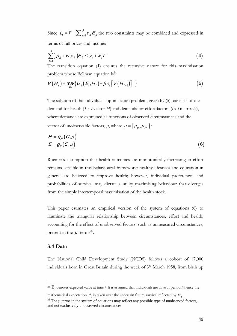
49

Since 1

Jt jt jtj

L T Eτ=

= −∑ the two constraints may be combined and expressed in

terms of full prices and income:

( ) ( )1

4J

jt t jt jt t tj

p w E y w Tτ=

+ ≤ +∑The transition equation (1) ensures the recursive nature for this maximisation

problem whose Bellman equation is24:

( ) { ( ) ( ) } ( )1max , 5t

t t t t t tEV H U E H V Hβ +⎡ ⎤= + Ε ⎣ ⎦

The solution of the individuals’ optimisation problem, given by (5), consists of the

demand for health (1 x t vector H) and demands for effort factors (j x t matrix E),

where demands are expressed as functions of observed circumstances and the

vector of unobservable factors, µ, where ,U Hµ µ µ= ⎡ ⎤⎣ ⎦ :

( )( ) ( )

,, 6

H

E

H g CE g C

µµ

=

=

Roemer’s assumption that health outcomes are monotonically increasing in effort

remains sensible in this behavioural framework: healthy lifestyles and education in

general are believed to improve health; however, individual preferences and

probabilities of survival may dictate a utility maximising behaviour that diverges

from the simple intertemporal maximisation of the health stock.

This paper estimates an empirical version of the system of equations (6) to

illuminate the triangular relationship between circumstances, effort and health,

accounting for the effect of unobserved factors, such as unmeasured circumstances,

present in the µ terms25.

3.4 Data The National Child Development Study (NCDS) follows a cohort of 17,000

individuals born in Great Britain during the week of 3rd March 1958, from birth up

24 Εt denotes expected value at time t. It is assumed that individuals are alive at period t, hence the

mathematical expectation Εt is taken over the uncertain future survival reflected by σ t . 25 The µ terms in the system of equations may reflect any possible type of unobserved factors, and not exclusively unobserved circumstances.

50

until age 46. The cohort members’ parents were interviewed for the first time in

1958 and extensive medical data on the children were collected; comprehensive

information about the cohort-members’ parental background, childhood health and

educational achievement was compiled during the first three waves of the study.

From wave four onwards, the NCDS questionnaires were addressed to the cohort

members and cover a broad range of subjects encompassing employment, health

and health-related behaviour, education, citizenship and values, parenting and

housing26.

Three separate health outcomes are used in the paper. The first is self-assessed

health (SAH) at age 46, measured on a five-point scale: excellent, good, fair, poor

and very poor health. SAH is widely used in health economics and has been shown

to predict mortality and deterioration of health even after controlling for the

medical assessment of health conditions; Idler and Kasl (1995) provide an extensive

literature review on this issue. In the specific case of the NCDS, the use of SAH is

also corroborated by its high correlation with reported disability and number of

hospitalisations27. The second health outcome is an indicator variable for whether

the individuals report to suffer from a long standing illness or disability at age 46.

The third health outcome used in the paper is an index of mental illness:

respondents answer a series of questions from the Cornell Medical Index

Questionnaire, each targeting a particular mental ailment; the number of positive

answers given at age 42 is then used as a malaise score, along the lines of Carneiro

et al. (2007).

Three main categories of circumstance variables are used in the paper: parental

socioeconomic background; congenital and childhood health of the cohort

members; cognitive ability, social development in childhood and educational

achievement. In terms of parental background, the NCDS contains rich information

26 The issue of attrition has been considered both in research papers and in reports produced by the NCDS advisory panel. Attrition does not appear to be associated with socioeconomic status, as shown in Case et al. (2005), and has modest positive correlation with cohort members’ unemployment as reported by Lindeboom et al. (2006). In this paper, a variable addition test was carried-out to investigate whether health-related attrition is a problem: ordered probit regressions were used to ascribe whether being in subsequent waves of the panel is a determinant of health status. The results show that, after controlling for a rich set of regressors, the fact that an individual is observed in subsequent waves of the NCDS is not significantly associated with their self-assessed health. 27 See Case et al. (2005, pp. 370).

51

that allows tracing the social class and years of schooling of the parents and of both

grandfathers of cohort members. Along the lines of Case et al. (2005) and

Lindeboom et al. (2006), this information is complemented by data on the incidence

of financial difficulties during cohort members’ childhood.

Cohort members’ childhood health is characterised by a set of morbidity measures,

aggregating twelve categories of acute and chronic health conditions, constructed

according to Power and Peckham (1987). Indicator variables for the occurrence of

diabetes, epilepsy and chronic heart conditions in parents and siblings are also

included in order to account for the incidence of hereditary conditions. Finally,

obesity at age 16 and parental smoking during the cohort members’ childhood and

adolescence are also treated as circumstances.

Recent research has provided evidence of a long term direct effect of cognitive

ability and social development in childhood on a wide range of behaviours in

adulthood with potential impacts on health28. These factors are largely beyond

individual control, hence can be regarded as circumstances. Scores of ability tests

taken at age 11 are used as proxies of cognitive ability, covering three fundamental

dimensions: mathematics, reading, and general ability. These test scores are highly

correlated at the individual level, leading to multicolllinearity in the econometric

models. To avoid this problem, the paper follows the approach of Galindo-Rueda

et al. (2005), using principal components analysis of the test scores to construct a

single measure of cognitive ability based on the first principal component.

To measure social development in childhood the paper uses scores of the Bristol

Social Adjustment Guide (BSAG), following Carneiro et al. (2007). These are used

as measures of social maladjustment at age 11: teachers are asked whether the child

has problems in twelve behavioural domains such as hostility towards children and

adults, anxiety, withdrawal, ‘writing off’ adults, unforthcomingness, depression,

restlessness, acceptance by adults, inconsequential behaviour and miscellaneous

psychological and nervous symptoms. One point is attributed to each positive

answer; the points are then summed to obtain the BASG social maladjustment

score.

28 See Heckman et al. (2006), Carneiro et al. (2007) and references therein.

52

The paper also treats as circumstances the highest educational qualifications attained

by the cohort members, since these are likely to be decisively influenced by parental

and environmental factors29. Cumulative indicator variables are used to categorise

the highest educational qualifications obtained: no formal qualifications; Certificates

of Secondary Education (CSE), O-levels or higher qualification; A-levels or higher

qualification; university degree or equivalent30.

The effort factors considered in the paper are health-related lifestyles. These may be

constrained by circumstances, but also reflect individual choices. The paper uses self

-reported individual data on cigarette smoking and on the consumption of alcohol

and fried food. Cigarette smoking is proxied by an indicator variable for whether

the individual is a smoker at age 33. Alcohol consumption is measured by the

number of units of alcohol consumed on average per week at age 33. NCDS

respondents are asked about their weekly consumption of a wide range of alcoholic

drinks (glasses of wine, pints of beer and so forth). These are then converted to

units of alcohol using the UK National Health Service (NHS) official guidelines31.

The consumption of fried food is measured by a categorical variable reflecting its

frequency in the individuals’ weekly diet at age 33. It should be noted that health

outcomes are measure either at age 46 or at age 42, but effort factors are measured

at age 33, so as to rule-out reverse causality due to a direct effect of the current

health status on behavioural choices.

3.5 Methods The empirical formulation of the model consists of a one-period version of the

system of reduced form equations (6) in which health outcomes and each of the

effort factors depend solely on circumstances and unobserved factors. Health is

represented by a vector with three components (SAH; long term illness and

29 In Chapter 2 the alternative approach is taken: instead of being treated as a circumstance, educational attainment is treated as an effort factor. That approach, is also defendable, since it is possible to postulate that, despite the influence of circumstances, there may remain an important element of individual free choice that needs to be taken into account. 30 CSEs and O-level (Ordinary levels) were secondary education qualifications corresponding, typically, to 11 years of education. A-levels (Advanced levels) are a qualification which corresponds to 13 years of education. Completion of A-levels is ordinarily a prerequisite for university admission. 31 These are publicly available at: http://www.nhsdirect.nhs.uk/magazine/interactive/drinking/index.aspx .

53

disability; mental illness) and effort by a vector composed of three lifestyles

(cigarette smoking; weekly consumption of fried food; weekly consumption of

alcohol).

This system is estimated by full information maximum likelihood, allowing the

system error terms to be freely correlated so as to account for unobserved common

factors that impact simultaneously on health and effort factors. This method of

dealing with selection on unobservables has been implemented in recent papers

such Pudney and Shields (2000), Vera Hernandez (2003), Deb and Trivedi (2006),

and Balia and Jones (2008), but not yet in the literature on inequality of opportunity.

However, as made clear by Roemer (2004), Lefranc et al.(2009) and Fleurbaey

(2008, p.240), accounting for this type of heterogeneity should be important in this

context since, in practice, it is often impossible to observe the entire set of relevant

circumstances likely to influence the outcome of interest. Although the theoretical

bounds for the error incurred through partial observation of circumstances have

not been derived, the several types of bias arising from this in the estimation and

measurement of inequality of opportunity are known as the partial-circumstance

problem and extensively discussed in Fleurbaey (2008, p.240-241).

The equations for SAH and for the consumption of fried food are estimated using

ordered probit models. The models for the incidence of long standing illness and

cigarette smoking are probits, and the equations for mental illness and alcohol

consumption are linear regressions. Multivariate normality of the error terms is

assumed and, given that the estimation of this system requires computation of

multidimensional integrals, a maximum simulated likelihood procedure is

implemented using the Geweke-Hajivassiliou-Keane (GHK) simulator32. The

system is intrinsically non-linear and hence identified by the set of functional

assumptions on the error term.

3.6 Results The importance of unobserved factors, which simultaneously affect both health

outcomes and lifestyles choices, can be evaluated by examining the estimates of the

32 Practical implementation was carried out using the Stata module cmp. Full details on this Stata module can be found in Roodman (2009).

54

correlation coefficients between the error terms of the system equations that are

shown in Table 1. The correlation coefficients between the errors of the SAH

equation and those of the equations for the incidence of long standing illness and

disability and for mental illness are negative and statistically significant; this indicates

the existence of unobserved factors that exert a positive effect on SAH and which,

simultaneously, reduce the incidence of long standing illness and mental health

conditions. The correlation between the error terms of the equation for long

standing illness and disability and of the equation for mental illness are positive and

statistically significant, due to third factors that favour the occurrence of both types

of health problems.

The correlation coefficients between the equation for cigarette smoking and the

equations for the consumption of fried food and alcohol are positive and

statistically significant. This is in line with evidence that suggests the existence of an

individual (genetic or otherwise) propensity for addictive behaviours, affecting

simultaneously the three detrimental lifestyles considered in the system.

Furthermore, the correlation between the error terms of the equations for SAH and

for each of these lifestyles is negative and statistically significant, confirming the

presence of unobservables that increase the probability of reporting good health

and that, at the same time, reduce the likelihood of individuals smoking, dinking

alcohol and consuming fried food. Finally, there are also unobserved factors that

jointly increase the incidence of mental illness and the consumption of alcoholic

drinks and cigarettes. These estimated correlations corroborate fully the relevance

of the partial-circumstance problem put forward in Fleurbaey (2008), highlighting

the vital importance of dealing with unobserved heterogeneity in the context of

inequality of opportunity. Previous work, such as Trannoy et al. (2009) and Rosa

Dias (2009), do not take this into account.

The estimated marginal effects33 for the one-period version of the system of

equations (6) are shown in Table 2. The estimates for the SAH equation are in line

with the previous literature that examines inequality of opportunity using self-

assessed health as the only proxy for health status in adulthood. After controlling

33 The marginal effects for the health equation are computed for the probability of reporting excellent health. The marginal effects for the equation for the consumption of fried food correspond to the probability of reporting to “eat fried food every day, more than once per day”.

55

for social class in adulthood, the cohort-members whose father was in the top

occupational category in 1958 are 6.2 percentage points more likely to report

excellent health at age 46 than those whose father was in the bottom social class.

This partial effect is 4.3 percentage points for those whose father was in the middle

social class. The incidence of childhood morbidities and the prevalence of chronic

illnesses such as epilepsy in the family have a large negative effect on SAH in

adulthood, in line with evidence provided by Case et al. (2005). Also in line with the

previous literature, obesity in adolescence is responsible for a 6 percentage points

reduction in the probability of reporting excellent health at age 46.

Educational qualifications are also positively associated to the probability of

reporting excellent health in adulthood. Conversely, there is a negative and

statistically significant effect of social maladjustment at age 11 on SAH at age 46,

after controlling for cognitive ability and for the highest academic qualifications

attained. Although this circumstance factor has received little attention in the

literature on inequality of opportunity, this result is in line with evidence provided

by Heckman et al. (2006) on the large impact of non-cognitive skills and social

development in childhood on a wide range of outcomes and behaviours in

adulthood.

The general pattern of how circumstances influence health outcomes changes

considerably once alternative components of the health vector are considered.

Contrary to the results obtained for SAH, parental social class, education and

household finances do not have a statistically significant effect on the incidence of

long standing illness and disability at age 46. This is mainly determined by gender,

with males being 5 percentage points more likely to be affected by these conditions,

childhood health and by a strong hereditary component: individuals in whose close

relatives suffer from epilepsy are 7 percentage points more likely to have developed

a chronic illness at age 46; this difference is of roughly 12 percentage points for

cohort-members whose close relatives suffer from chronic heart disease. Social

maladjustment at age 11 is also positive and statistically significantly associated with

the development of chronic illness in adulthood. Finally, the NCDS cohort

members who are in the top social class in adulthood are approximately 5

56

percentage points less likely to suffer from a long standing illness at age 46 than

those in the bottom social class.

The estimates for the occurrence of mental illness at age 46 also follow a different

pattern of influence to SAH, with parental social class found not to be statistically

significant. At age 46, the male cohort-members are less likely to report mental

health problems than females. The incidence of these has a positive and statistically

significant association with poor childhood health and with the prevalence of

chronic conditions in close relatives. Social maladjustment in childhood has a

statistically significant positive impact on mental illness in adulthood. Educational

attainment has a protective effect: the completion of O-levels or of a higher

qualification has a strong and statistically significant negative association with the

occurrence of mental health conditions at age 46.

These results show that while the three elements of the health vector are strongly

affected by unfair circumstances, each of them responds to a different subset of

circumstance factors. In particular, parental socioeconomic status and parental

education have a decisive effect on SAH at age 46 but no statistically significant

association with the remaining health outcomes.

The remaining three equations of the system concern effort factors. The first of

these is a probit model for the probability of an individual being a smoker at age 33.

This has a statistically significant association with parental smoking, but not with

parental socioeconomic status. Social maladjustment in childhood and differences in

educational achievement play a key role in explaining differences in the probability

of smoking in adulthood: cohort-members who obtained O-levels or a higher

qualification are 9.3 percentage points less likely to smoke at age 46 than those

without formal qualifications, after controlling for a wide set of childhood

circumstances, ability and social class in adulthood. This corroborates results from

the previous literature suggesting that complementary policies in the education

sector may be crucial for reducing inequality of opportunity in health. There is also

a clear socioeconomic gradient in the probability of smoking: those in the top social

class in adulthood are roughly 6 percentage points less likely to be smokers than the

cohort members in the bottom social class.

57

The fifth equation in the system is an ordered probit for the weekly frequency of

the consumption of fried food. The estimated marginal effects show gender

differences: male cohort members are around 4 percentage points more likely to

consume fried food every day than females. Similar to the case of cigarette smoking,

there is no statistically significant association between parental social class and the

consumption of fried food. Obesity at age 16 has a negative and statistically

significant effect on the consumption of fried food: on average, individuals who

were obese in adolescence are 1.2 percentage points less likely to consume fried

food every day than those who were not. This is in line with the rationale of

individual offsetting of health risks in the face of perceived frailty. It also confirms

that the harmful impact of childhood obesity on adult health is mainly a direct one,

which does not operate solely through dietary choices in adulthood; this favours

tacking childhood obesity as a policy objective in its own right.

Educational achievement is also found to have a negative impact on the

consumption of fried food: individuals who attained O-levels or a higher

qualification are approximately 1.5 percentage points less likely to eat fried food on

a daily basis than the cohort members without formal qualifications. In addition, the

results provide evidence of a negative association between this lifestyle and high

socioeconomic status in adulthood: the cohort members in the top social class at

age 42 are nearly 1 percentage point less likely than those in the bottom social class

to consume fried food daily.

Finally, the estimates for the weekly consumption of alcohol at age 33 show that

gender differences are decisive with respect to this lifestyle: males are associated

with a much higher consumption of alcohol than females. The estimates show

neither an association between parental social class at birth and the consumption of

alcohol in adulthood, nor a clear gradient defined in terms of the individuals’

educational qualifications and social class in adulthood. The results also do not

provide evidence of an ability gradient: both cognitive ability and social

maladjustment in childhood show a positive and statistically significant association

with the consumption of alcohol at age 33.

58

3.7 Discussion and conclusions

This paper develops a behavioural model of inequality of opportunity in health in

which lifestyle choices are the consequence of a utility maximising behaviour

subject to constraints. This integrates John Roemer’s framework of inequality of

opportunity with the Grossman model of health capital and demand for health. The

model generates a recursive system of equations for health and lifestyles which is jointly

estimated by full information maximum likelihood with freely correlated error terms. The

purpose of this approach is twofold. First, it sheds light on the triangular

relationship between circumstances, effort and health. Second, it addresses the

problem posed by partial observability of the relevant set of circumstances, known

as the partial-circumstance problem.

The results indicate the presence of unobserved factors that impact simultaneously

on the various health outcomes and effort factors considered in the system; this

confirms the crucial importance of taking into account unobserved heterogeneity in

a context of partially observed circumstances. This aspect, widely discussed in the

theoretical literature, has been ignored in earlier empirical work on inequality of

opportunity; it is therefore a promising avenue for further research.

Taking into account the effect of these unobserved factors, the system estimates for

SAH at age 46 corroborate the key results of the existing literature on inequality of

opportunity in health, which is almost exclusively focused on this health outcome.

SAH in adulthood is strongly impacted by circumstances such as parental

socioeconomic status and childhood health conditions, establishing the existence of

inequality of opportunity. However, once alternative health outcomes are

considered, such as the incidence of long standing illness, disability and mental

health problems, the pattern of inequality of opportunity changes substantially, with

no role for parental social class and education in the determination of these health

outcomes in adulthood. While the three elements of the health vector are strongly

affected by unfair circumstances, each of them responds to a different subset of

circumstance factors.

59

Finally, the results also show that circumstances affect health outcomes both

directly and indirectly, through their effect on effort. An important example relates

to social development in childhood and educational qualifications, which have

important implications for the lifestyle choices considered in this paper. This

corroborates evidence from earlier literature, suggesting that complementary

policies in the educational sector may be key to reducing health inequalities.

60

Appendix B Table 1: System errors correlation matrix

System equations Rho Std. Dev.SAH / Long standing illness -0.534*** 0.032SAH / Mental illnesss -0.267*** 0.023SAH / Smoker -0.181*** 0.034SAH / Consumption of fried food -0.07*** 0.024SAH / Alcohol consumption -0.051** 0.023Long standing illness / Mental illness 0.205*** 0.026Long standing illness / Smoker -0.034 0.040Long standing illness / Consumption of fried food -0.025 0.029Long standing illness / Alcohol consumption -0.034 0.028Mental illness / Smoker 0.068** 0.029Mental illness / Consumption of fried food 0.021 0.021Mental illness / Alcohol consumption 0.058*** 0.022Smoker / Consumption of fried food 0.177*** 0.032Smoker /Alcohol consumption 0.146*** 0.031Consumption of fried food / alcohol consumption 0.032 0.023

61

Table 2: System estimates (empirical version of the system of equations denoted (6) in Section 3)

Coefficient Marg. Eff. Coefficient Marg. Eff. Coefficient Marg. Eff. Coefficient Marg. Eff. Coefficient Marg. Eff. Coefficient Marg. Eff.Male 0.035 0.013 0.153*** 0.052 -0.678*** -0.678 -0.149 -0.03 0.646*** 0.0330 16.627*** 16.627

(0.0461) (0.055) (0.126) (0.062) (0.046) (1.544)Parental SES at birth: High 0.167** 0.061 -0.107 -0.036 -0.017 -0.017 -0.15 -0.038 -0.098 -0.0040 2.545 2.545

(0.0745) (0.089) (0.206) (0.101) (0.072) (2.045)Parental SES at birth: Middle 0.119* 0.043 -0.078 -0.027 0.069 0.069 -0.075 -0.019 -0.051 -0.0020 2.393 2.393

(0.065) (0.076) (0.173) (0.082) (0.06) (1.782)Years of education: Father -0.015 -0.005 -0.012 -0.004 0.049 0.049 -0.0002 -0.005 0.006 0.0003 0.167 0.167

(0.0171) (0.02) (0.05) (0.024) (0.018) (0.517)Years of education: Mother 0.018 0.006 -0.031 -0.010 0.008 0.008 0.08** 0.021 0.052** 0.0026 -0.321 -0.321

(0.0192) (0.023) (0.055) (0.025) (0.019) (0.583)Financial hardship (age 11) -0.121 -0.043 0.005 0.001 0.41 0.41 0.06 0.017 -0.0002 0.0000 1.466 1.466

(0.104) (0.131) (0.263) (0.138) (0.099) (2.707)Physical/mental impairments (age 16 -0.059*** -0.021 0.060*** 0.020 0.149*** 0.149 -0.009 -0.002 -0.014 -0.0007 0.233 0.233

(0.0180) (0.021) (0.046) (0.024) (0.017) (0.5)Number of hospitalisations (age 11) -0.054 -0.019 0.029 0.010 0.032 0.032 0.016 0.004 -0.001 -0.0001 -0.475 -0.475

(0.0383) (0.045) (0.1) (0.05) (0.036) (1.07)Diabetes in parents or siblings -0.134 -0.047 -0.053 -0.018 -0.152 -0.152 -0.08 -0.022 0.018 0.0009 0.898 0.898

(0.137) (0.191) (0.452) (0.211) (0.147) (4.52)Epilepsy in parents or siblings -0.170** -0.060 0.196* 0.070 -0.022 -0.022 0.15 0.041 0.016 0.0008 -0.442 -0.442

(0.086) (0.107) (0.243) (0.117) (0.085) (2.723)Chronic heart disease -0.080 -0.028 0.322* 0.119 1.009** 1.009 -0.279 -0.064 -0.01 -0.0005 -0.887 -0.887

(0.142) (0.174) (0.411) (0.262) (0.164) (4.5)Mother smoker (age 16) -0.007** -0.002 -0.002 -0.001 0.014 0.014 0.016*** 0.004 0.00008 4.42e-06 0.023 0.023

(0.003) (0.003) (0.008) (0.004) (0.003) (0.092)Obesity (age 16) -0.176 -0.061 0.105 0.037 -0.035 -0.035 0.228 0.065 -0.307*** -0.0120 -2.749 -2.749

(0.111) (0.134) (0.299) (0.142) (0.106) (3.254)Cognitive abiliy (age 11) 0.006 0.002 -0.009 0.000 0.03 0.03 0.018 0.004 0.01 0.0005 1.612*** 1.612

(0.020) (0.024) (0.054) (0.026) (0.019) (0.595)Social development (age 11) -0.007*** -0.002 0.008** 0.003 0.03*** 0.03 0.0187*** 0.004 0.001 0.0001 0.131* 0.131

(0.002) (0.003) (0.007) (0.003) (0.002) (0.0792)University degree or equivalent -0.038 -0.014 -0.037 -0.01 -0.149 -0.149 -0.171 -0.042 -0.054 -0.0020 -2.5 -2.5

(0.077) (0.095) (0.234) (0.121) (0.081) (2.285)A-levels or higher qualification 0.108* 0.039 0.06 0.02 -0.29 -0.29 -0.251** -0.06 -0.14** -0.0060 -1.527 -1.52

(0.112) (0.085) (0.204) (0.1009) (0.071) (1.959)O-levels or higher qualification 0.084 0.030 0.004 0.00 -0.356** -0.356 -0.32*** -0.093 -0.252*** -0.0154 -2.443 -2.443

(0.079) (0.095) (9.193) (0.099) (0.071) (2.048)Own socioeconomic status: High† 0.243*** 0.088 -0.155* -0.05 -0.133 -0.133 -0.235** -0.061 -0.143** -0.0070 0.087 0.087

(0.078) (0.091) (0.206) (0.102) (0.074) (2.178)Own socioeconomic status: Middle† 0.258*** 0.094 -0.112 -0.04 -0.093 -0.093 -0.039 -0.01 0.008 0.0004 0.031 0.031

(0.074) (0.086) (0.186) (0.093) (0.068) (2.089)Constant -0.255 2.88 2.88 -1.09*** 22.729*** 22.729

(0.282) (0.599) (0.312) (6.987)

Number of observations: 2665

Notes: Standard errors in parentheses; *** p<0.01. ** p<0.05. * p<0.1. Coefficients and marginal effects for regional variables are suppressed here (due to statistical insignifiance) but available upon request.† at age 33.

SAH(OLS estimates)(Ordered probit estimates) (Probit estimates) (OLS estimates) (Probit estimates) (Ordered probit estimates)

AlcoholMental illness

Dep. Variable Dep. Variable Dep. Variable Dep. Variable Dep. Variable Dep. Variable

Indicator: SmokerLong standing illness /

disability Fried food

62

Chapter 4

Quality of Schooling and Inequality of Opportunity in Health

4.1 Introduction

Recent empirical work, such as Trannoy et al. (2009) and Rosa Dias (2009), suggests

that differences in education are a leading cause of inequality of opportunity in

health. This is in line with the earlier literature on socioeconomic inequalities in

health, such as Wagstaff, van Doorslaer and Watanabe (2003) and van Doorslaer

and Jones (2003), and agrees with the large body of evidence emphasising the role

of complementary educational policies in reducing long-run health inequalities.

The issue of complementary policies has been brought to the fore in various fields

of economics, and the reciprocal association between health and education policy

has attracted particular attention. First, the way childhood health constitutes a pre-

requisite for the success of educational policy is well documented in empirical

papers such as Mayer-Foulkes (2001), Miguel (2005), Alderman et al (2006),

Contoyannis and Dooley (2010), in the official guidelines of policy makers (for

example the World Food Program (2006)) and in theoretical models of child

nutrition and human capital formation, such Currais et al. (2010) and De la Croix

and Doepke (2003). Second, the fact that education is a vital input in the health

production function has been established by papers such as Lleras-Muney (2005),

Arendt (2005; 2008), Oreopoulos (2006), Silles (2009) and Van Kippersluis et al.

(2009); these provide evidence of the existence of positive long term health effects

of successive increases in the number of years of compulsory education in Europe

and in the USA.

Cutler and Lleras-Muney (2010) recently added to this body of evidence by carrying

out an empirical assessment of the most common explanations for the relationship

between years of schooling and the wide disparities observed in individual health

63

related behaviours. Nonetheless, this literature leaves important questions

unanswered. One of such questions underlined in Cutler and Lleras-Muney (2008,

p.22), concerns the existence of health returns to different qualities of education.

This is a topical policy issue, since evidence on the existence of such returns is vital

to inform the design of complementary policy interventions connecting the

educational and the healthcare sectors. This paper seeks to narrow this gap. We

adapt the empirical strategy put forward by Cutler and Lleras-Muney (2010) to

examine the association between quality of schooling and health inequalities in

adulthood. This is done by exploiting the wide variation in quality of the primary

and secondary schools attended by cohort-members of the National Child

Development Study (NCDS). We address three main issues:

• Whether, from a normative standpoint, there is inequality of opportunity in

health by quality of education among NCDS cohort-members.

• The existence of a statistical association between quality of schooling and

health and lifestyle in adulthood.

• The identification of channels that mediate this association.

The NCDS cohort-members’ educational experience has some distinct features,

both at primary and secondary levels. To begin, some of them attended state

primary schools while others went to private primary schools; these schools were

typically different in terms of available resources, peer effects, and curricula.

Nonetheless, the main source of variability in the cohort members’ quality of

schooling relates to the very different types of secondary schools attended. This is

mainly due to the fact that the cohort’s secondary schooling years lie within a

transition period corresponding to the major comprehensive schooling reform,

implemented in England and Wales34. The reform was not introduced

simultaneously nationwide. Some pupils were unaffected by it and attended the pre-

existing, highly selective state-funded tri-partite system, which comprised grammar

schools, secondary modern schools and a small and declining number of technical

34 Data on Scotland are not used: the Scottish educational system of the 1960’s and 1970’s was structurally very different from the one experienced by all the other NCDS cohort-members, and comprehensive schooling was introduced earlier, preventing a legitimate comparison of types of school, educational qualifications and outcomes.

64

schools. The majority of the cohort was affected by the reform and attended

comprehensive schools. Also, a minority of NCDS cohort went to private fee-

paying schools, independent of the state schools educational systems and reforms.

The distribution of the NCDS cohort members by type of secondary school is

shown in Figure 1.

4.2 Quality of schooling

4.2.1 Primary education

Table 1 shows the breakdown of the type of primary education experienced by the

NCDS cohort-members, by type and characteristics of the schools. The mean pupil-

teacher ratios were different between state and private schools and their

distributions were markedly dissimilar, as made clear in Figure 2, which contrasts

state with private primary schools. The effect of these differences on educational

attainment and wages was examined using NCDS data by Dearden, Ferri and

Meghir (2005). However, their effect on health-related behaviours and outcomes

has not been taken into account by the existing literature.

4.2.2 Secondary education: the comprehensive reform and equality of opportunity

As shown in Figure 1, nearly 40 per cent of the state schools students were not

affected directly by the reform and attended the tri-partite system of state-funded

education. Grammar schools were academically oriented state schools that provided

teaching for the entire age range 11-18, including a sixth form for Advanced level

(‘A-level’) studies, and prepared pupils to go on to higher education. Admission into

these schools was determined by an exam taken at age 11 (the ‘Eleven Plus’ exam).

Pupils whose examination score did not permit entry into a grammar school went to

secondary modern schools, which were also state schools, but less academically

oriented and covered the ages 11-16 or, in a small minority of cases, vocational

schools aimed at providing training and technical apprenticeships35.

35 In a few cases, pupils whose grades were sufficient transferred to grammar schools or sixth form colleges to complete their A-levels.

65

A substantial share of the cohort members were affected by the reform, which was

explicitly designed to promote equality of opportunity between children of different

parental backgrounds. The reform replaced the selective educational system (both

grammar and secondary modern schools) by a unified mixed ability secondary

schools system (“comprehensive schools”) 36. The types of schools were

substantially different in their curriculum, examinations, and academic environment

and peer effects. Table 2 shows that, among the schools attended by the NCDS

cohort members at age 16, 79 per cent of private schools and 68 per cent of

grammar schools were single sex, while only 13 per cent of comprehensives were

single sex. Streaming of classes by academic ability was common in secondary

moderns and comprehensives but rare among grammar schools. Some

comprehensives were former secondary moderns (18 per cent) or grammar schools

(25 per cent) with rest being newly created. Furthermore, the distribution of the

pupil-teacher ratio also differs considerably across these four types of schools as

shown in Figure 3.

4.3 Data The National Child Development Study (NCDS) follows a cohort of nearly 17,000

individuals, who were born in Great Britain in the week of 3rd March 1958, from

birth up until age 46. Seven waves of interviews have been carried-out when cohort

members were 7, 11, 16, 23, 33, 42 and 46 years old. The study compiles in-depth

information on the cohort-members’ childhood health and parental background. It

comprehensively records cognitive ability and social development in childhood and

adolescence, and, crucially for this paper, quality of schooling at primary and

secondary levels together with overall educational achievement. It also includes

measures of social status in adulthood, and detailed information on health-related

behaviours and health outcomes in adulthood.

4.3.1 Childhood health, parental background and neighbourhood characteristics

36 Following much controversy over the Eleven Plus, the selective system went into decline in the 1960’s and 1970s, until it was abolished in England and Wales by the 1976 Education Act. The selective system has persisted in certain areas, such as Kent.

66

The NCDS data include extensive information on the cohort-members’ early health

endowments. In order to control for these we have constructed morbidity measures

that aggregate twelve categories of health conditions affecting the child at ages 7

and 11 (following Power and Peckham, 1987). We have also created indicator

variables for the occurrence of diabetes, epilepsy and other chronic conditions in

parents and siblings in order to account for the incidence of hereditary conditions in

the cohort members’ family. NCDS data on the height and weight of the cohort-

members also allows us to control for the long-term impact of obesity in childhood

and adolescence.

In terms of parental background, the NCDS allows us to trace the social class and

the years of schooling of both parents of the cohort members. Following Case et al.

(2005) and Lindeboom et al. (2009), we have complemented this information with

data on the incidence of household financial difficulties during the cohort member’s

childhood and adolescence.

The NCDS also includes rich information about the socioeconomic characteristics

of the cohort-members’ neighbourhood during childhood and adolescence. For the

years of 1971 and 1981, NCDS survey data was linked to census data37; this makes it

possible to use census enumeration district level data (the smallest unit for which

census statistics are available with an average population of about 460) to control

for geographic heterogeneity in the individual’s immediate social milieu.

4.3.2 Cognitive ability, social development and educational achievement

The NCDS is rich in measures of cognitive and social development prior to

secondary schooling. Scores of ability tests taken at ages 7 and 11 are available on a

series of cognitive dimensions: mathematics, reading, copying designs and general

ability. Since test scores are highly correlated, hence leading to multicollinearity in

econometric models, we follow Galindo-Rueda et al. (2005) and use principal

components analysis to construct a single measure of cognitive ability using the first

37 This small are data are available under a special licence, which imposes restrictions on the handling and usage of the data. Details can be found at http://www.cls.ioe.ac.uk/studies.asp?section=0001000200030015.

67

principal component. We use as controls both the individuals’ measure of cognitive

ability and their relative rank in the distribution of cognitive ability of their peers.

Social development has received growing attention as an explanatory factor for

behaviour, competence and achievement in adulthood. Following Carneiro et al.

(2007) the score for the Bristol Social Adjustment Guide (BSAG) is used as a

measure of social development at age 11: teachers are asked whether the child has

problems in twelve behavioural domains such as hostility towards children and

adults, anxiety, withdrawal, ‘writing off’ adults, unforthcomingness, depression,

restlessness, acceptance by adults, inconsequential behaviour and miscellaneous

psychological and nervous symptoms. One point is attributed to each positive

answer; points are then summed to obtain the BASG social maladjustment score.

The distribution of both cognitive and non-cognitive ability measures is shown in

Figure 4.

The NCDS also includes information on the educational attainment and

qualifications awarded to cohort members: no formal qualifications; Certificates of

Secondary Education (CSE), O-levels, A-levels and university degree or

equivalent38. We further disaggregate this information on educational achievement

into twelve categories, ordered according to the grades obtained and number of

passes.

4.3.3 Health-related behaviours, attitudes and outcomes

The NCDS contains self-reported information on a series of health-related

lifestyles: cigarettes smoked per day, average units of alcohol consumed per week39

and dietary choices, such as the frequency of consumption of fried food, vegetables

and sweets. These data are only available in the four most recent waves of the study,

once respondents are aged 23 and above. We also look at other health-related

38 CSEs and O-level (Ordinary levels) were secondary education qualifications corresponding, typically, to 11 years of education in total; CSEs were academically less demanding than O-levels. A-levels (Advanced levels) are a qualification which typically corresponds to 13 years of education. Completion of A-levels is ordinarily a prerequisite for university admission. 39 NCDS respondents are asked about their weekly consumption of a wide range of alcoholic drinks (glasses of wine, pints of beer and so forth). These are then converted to units of alcohol using the UK National Health Service official guidelines that are available at: http://www.nhsdirect.nhs.uk/magazine/interactive/drinking/index.aspx .

68

behaviours among women, such as teenage pregnancy and maternal smoking during

pregnancy, susceptible of being affected by qualitative aspects of education.

The effect of quality of schooling is examined for a range of health outcomes in

adulthood and late adolescence. The first of these is self-assessed health (SAH),

measured on a five-point scale: excellent, good, fair, poor and very poor health.

SAH is widely used in health economics and has been shown to predict mortality

and deterioration of health even after controlling for the medical assessment of

health conditions.

A more specific measure of health in adulthood is the incidence self-reported long

standing illness or disability at age 46. Information on the particular medical

condition associated with it is available and classified according to the International

Classification of Diseases (ICD-10).

Mental health in adulthood is taken into account as a separate outcome: NCDS

respondents answer to a series of questions from the Cornell Medical Index

Questionnaire, each targeting a particular mental ailment; the number of positive

answers given at age 42 is then used as a malaise score along the lines of Carneiro et

al. (2007).

4.3.4 Sample selection and non-response

The size of our final estimation samples was significantly affected by attrition and

especially by the patterns of item non-response. However, recent papers that

analyse NCDS data, such as Case et al. (2005) and Lindeboom et al. (2006),

recognise the problem but do not find evidence of non-random attrition. Table 3

contrasts the full NCDS sample with the estimation sample used in our

econometric analysis. On average, individuals in the estimation sample come from

slightly richer and better-educated backgrounds when compared with the full

sample. They score higher than the full sample in ability tests taken at age 11, but do

not have systematically better childhood health.

69

4.4 Methods We begin by using the stochastic dominance testable conditions defined in Chapter

2 (Section 2.2.2) to detect the presence of inequality of opportunity in health by

quality of schooling among NCDS cohort-members.Then we explore the existence

of a statistical association between quality of schooling and both health and lifestyle

in adulthood, adopting a similar approach to that of Cutler and Lleras-Muney

(2009).

4.4.1 Inequality of opportunity in health

To examine the role of quality of schooling as a source of inequality of opportunity

in health we adopt the framework of Roemer (2002); this has been the workhorse in

most of the applied literature on inequality of opportunity in health. Roemer (2002)

sorts all factors influencing individual attainment between a category of effort factors,

for which individuals should be held partly responsible for and a category of

circumstance factors, which, being beyond individual control, are a source of unfair

differences in outcomes. In our case, we assume that the type of secondary school

in which pupils are enrolled at age 11 is largely beyond their individual control and

therefore constitutes a circumstance. Since the outcome of interest is a range of

health outcomes in adulthood (H), a generalised health production function can be

defined along the lines of Roemer (2002) as H (C, E(C)) , where C denotes

individual circumstances and E denotes effort, which is itself a function of

circumstances.

Roemer (2002) defines social types consisting of individuals who share exposure to

the same circumstances, for example the attendance at the same type of secondary

school. Roemer’s definition of equality of opportunity is that, on average, all those

who exert the same effort should be entitled to equivalent health status, irrespective

of their circumstances. Such a situation corresponds to a full nullification of the

effect of circumstances, keeping untouched the differences in outcome that are

caused solely by effort.

Denoting by F H | C( ) the cumulative distribution function of the health outcome of

interest conditional on circumstances, a literal translation of Roemer’s notion of

70

inequality of opportunity would mean considering that there is inequality of

opportunity whenever: ∀C ≠ C ', F H | C( )≠ F H | C '( ). This condition is however too

stringent to be useful in empirical work. Lefranc et al. (2009) consider that the data

are consistent with the hypothesis of inequality of opportunity if the social

advantage provided by different circumstances can be unequivocally ranked by first

degree stochastic dominance40 (FSD), i.e. if the distributions of health conditional

on different circumstances can be ordered according to:

( ) ( )', | | ' .FSDC C F H C F H C∀ ≠

We follow this literature, carrying out stochastic dominance tests to detect inequality

of opportunity in a series of health outcomes. The testable condition for inequality

of opportunity is therefore:

( ) ( ) school type A, school type B, |school type A |school type B .FSDF H F H∀

4.4.2 Regression analysis

We estimate, for each outcome of interest, a model of the form:

health outcomei , age46

= α + β1, i∗ (type and characteristics of school) + β

2, i∗ (childhood health) +

+β3, i∗ (ability prior to enrolment) + β

4, i∗ (parental background) + β

5, i∗ (local area / other control variables) + ε

i

By exploiting the rich set of covariates that are observed prior to enrolment we

control for most of the potential confounders of the relationship between quality of

schooling and health in adulthood. While potentially over-controlling, this

specification establishes a conveniently stringent test for the statistical significance

of the association in question.

40 A lottery stochastically dominates another if it yields a higher expected utility. Several orders of stochastic dominance may therefore be defined according to the restrictions one is willing to make on the individual utility function. First order stochastic dominance (FSD) holds for the whole class of increasing utility functions (u’>0); this corresponds to simply comparing cdfs of the earnings paid by alternative lotteries. Second order stochastic dominance (SSD) applies to utility functions which are increasing and concave in income, reflecting the notion of risk aversion (u’>0 and u’’<0); SSD evaluates integrals of the cdfs. While FSD implies SSD, the converse is clearly not true. SSD cannot be defined for discrete and ordinal outcomes such as the ones used in this paper, hence all definitions and tests refer to FSD.

71

We then estimate a sequence of models in order to illuminate three possible

mediating channels for this association: academic qualifications; lifestyles;

socioeconomic status in adulthood. The models that account for all of these for

each health outcome are of the form:

health outcomei ,age46

= α + β1,i∗ (type and characteristics of school) + β

2,i∗ (childhood health) +

+β3,i∗ (ability) + β

4,i∗ (parental background) + β

5,i∗ (local area / other control variables) +

+β6,i∗ (highest edu. qualificationage42 )+β

7,i∗ (lifestylesage33/42 )+ β

8, i∗ (social classage42 ) + ε

i

4.5 Results

4.5.1 Quality of schooling and inequality of opportunity in health

Within the framework of Roemer (2002), quality of schooling, at both primary and

secondary levels, constitutes a circumstance. A general picture of its association

with health is patent in Figure 5, featuring the possible pairwise comparisons

between the empirical distributions of SAH at age 46 by type of secondary

schooling. When we contrast the SAH profiles of individuals who attended

secondary modern and grammar schools, the gap between the two empirical

distributions is remarkably wide. This is striking since it is attributable to one single

circumstance. Conversely, the empirical distributions of SAH for grammar and

private schools are very similar; the same happens when we compare the SAH

profiles for comprehensive and secondary moderns. Figure 6 features the same type

of pairwise comparisons applied to the empirical distributions of the mental illness

index at age 46; the gaps are slightly less pronounced, but still striking.

72

In order to formally assess the existence of inequality of opportunity using the

formulation presented in Section 4.4.1, Kolmogorov-Smirnov tests for first degree

stochastic dominance are carried-out; the statistically significant results at the 1%

significance level are shown in Table 6. The results for SAH at age 46 establish four

statistically significant dominance relationships: the self-assessed health of cohort-

members who attended at grammar and private schools dominates the one of those

who went to secondary modern and comprehensive schools. For detrimental

outcomes, this pattern is reversed: secondary modern schools dominate grammar

schools for cigarette smoking and incidence of chronic disease and mental illness

and private schools for cigarette smoking and incidence of chronic diseases.

Comprehensive schools dominate grammar schools at first order for all the

detrimental outcomes and private schools for cigarette smoking only. These results

establish the existence of inequality of opportunity in health and health-related

outcomes, favouring the cohort members who attended at grammar and private

schools relatively to their counterparts who attended comprehensive and secondary

modern schools.

4.5.2 Quality of schooling, health and lifestyle: primary schools

Table 4 shows estimates of the association between primary school characteristics

and a series of health-related behaviours and outcomes in adulthood. Models 1 to 5

each add an additional set of control variables to the preceeding models. Model 1

includes the rich set of pre-schooling control variables described in Section 4.2 and

listed in Appendix D: parental socioeconomic status and education, childhood

health and local area characteristics (census enumeration district). Model 2 controls,

aditionally, for cognitive and non-cognitive ability, measured at age 7. Models 3, 4

and 5 add, respectively, three potential channels of the influence of quality of

schooling on health: lifestyle in adulthood, highest academic qualifications attained

and socioeconomic group at age 42. Table 4 displays partial effects on the outcomes

of interest, computed by averaging across all individual marginal effects in the

sample. Models for self-assessed health and for the weekly consumption of fried

food are ordered probit specifications; partial effects correspond, respectively, to

the probability of reporting excellent health and of consuming fried food on a daily

basis at age 46. For the smoking status, incidence of chronic illness, teenage

73

pregnancy and maternal smoking during pregnancy probit specifications are used.

Finally, the models for the Cornell index of mental illness and for the number of

weekly units of alcohol are linear regressions.

The results do not indicate a statistically significant association between schools

being privately owned and operated, teacher-pupil ratios, and self-assessed health at

age 46. However, the indicator variable for whether pupils were happy at primary

school is a good predictor of health in adulthood: after controlling for parental

background, cognitive ability and social development, lifestyle and academic

qualifications, dissatisfaction at primary school is associated with a nearly 6

percentage points reduction on the probability of reporting excellent health at age

4641. In terms of prevalence of long standing illness and disability, the partial effects

of private school indicators and teacher-pupil ratios remain statistically insignificant

and generally small. Also, the pattern of large and statistically significant partial

effects of unhappiness in primary school persists; their magnitude and precision are

however attenuated once the effects of overall educational achievement and social

class in adulthood are controlled for (models 4 and 5).

The results for mental illness at age 46 show a different pattern. There is a clear

negative and statistically significant association between the teacher-pupil ratio and

the prevalence of mental illness in adulthood. The size of the partial effects is

roughly constant across models, whence lifestyle choices, educational qualifications

and social status in adulthood are not the chief mediators of this relationship. Also,

although imprecise, the partial effects of attendance at a private primary school are

consistently positive and large in all models42. Once more, unhappiness at school is

strongly and positively associated with the incidence of mental illness at age 46 in all

the models considered. Social status in adulthood appears to be an important

channel for this association given that partial effects are reduced by nearly 30

percentage points once we control for the effect of social class.

41 As emphasised by the large literature on the harmful impact of bad parenting on human development, this association should not be interpreted as a causal effect, since dissatisfaction at school is likely to also reflect the lack of family-based support for schooling and early learning. 42 Reverse causality may be a possible explanation for this association if mentally troubled children were relatively more likely to benefit from smaller class size and to attend to private schools.

74

In the models for these three health outcomes, self-reported health, chronic and

mental disorders, the magnitude of the estimated partial effects does not change

much once lifestyle choices are controlled for, suggesting that health related

behaviours do not mediate the effect of quality of primary schooling on health

outcomes. This fact is corroborated by the estimates obtained for the models for

cigarette smoking and consumption of alcohol and fried food. In almost all cases,

the partial effects for the quality of school indicators are statistically insignificant

and economically negligible.

The results also provide no evidence of an impact of quality of primary education

on the occurrence of teenage pregnancies and on cigarette smoking during

pregnancy. Due to the smaller size of the estimation samples for the last two

outcomes of Table 4 none of the female cohort-members who attended at private

primary school reported to have smoked during their pregnancies; we therefore

dropped the indicator for private school from the last model of the table.

4.5.3 Quality of schooling, health and lifestyle: secondary schools

Table 5 presents the results for the relationship between quality of secondary

education and the same range of outcomes and health-related attitudes considered

in section 4.5.243. The main variables of interest are now indicators for the four

types of schools described above (comprehensive schools, secondary modern

schools, grammar schools, private schools), school characteristics and resources.

The reference category for the comparisons between types of school is attendance

at a grammar school, which, on average, is associated with the best health

outcomes.

43 Table 5 also shows partial effects on the outcomes of interest, computed by averaging across all individual marginal effects in the sample. Models for self-assessed health and for the weekly consumption of fried food are ordered probit specifications; partial effects correspond, respectively, to the probability of reporting excellent health and of consuming fried food on a daily basis at age 46. For the smoking status, incidence of chronic illness, teenage pregnancy and maternal smoking during pregnancy probit specifications are used. Finally, the models for the Cornell index of mental illness and for the number of weekly units of alcohol are linear regressions.The set of control variables included in Models 1 to 5 is the same as in Table 4.

75

The estimates in the table show no evidence of a statistically significant association

between types of schools and SAH at age 46: the negative association with

attendance at secondary modern schools, found in Model 1, disappears after

controlling for differences in cognitive ability and social development. The only

school characteristic that bears a negative and statistically significant association

with SAH at age 46 is the schools’ student expulsion rate. This variable is

commonly used as a proxy for the school’s academic environment and peer effects,

which potentially shapes lifestyle and preferences such as risk aversion and

subjective valuation of the future. Interestingly, however, the size of its estimated

partial effects is relatively constant across the five models, suggesting that its

association with health is not mediated by lifestyles, academic achievement, or social

status in adulthood.

The models for the incidence of chronic illness and disability show a different

pattern. Attendance at comprehensive and secondary modern schools is associated

with a higher incidence of chronic illness and disability than grammar schools. The

size of these effects is substantial: nearly 11 per cent higher incidence in the case

comprehensives and roughly 8 percentage points higher incidence in the case of

secondary moderns, when the full set of controls is included in the model. This

constitutes evidence of a large association between quality of schooling and health,

over and above the effect of educational qualifications, ability and lifestyle.

The association between the attendance at different types of schools and the

occurrence of mental illness in adulthood is also sizable and statistically significant.

In line with the results obtained for primary education, the partial effect of

attendance at private secondary schools is positive and large, after controlling for

the entire available set of covariates. The relative constancy of these partial effects

across the five models suggests once more that lifestyle quality and academic

qualifications are not channels for this relationship. Indicator variables for whether

these schools were single-sex schools and boarding schools are not statistically

significant.

76

Attendance at boarding schools is a perfect predictor of the two maternity-related

outcomes in Table 5: none of the cohort-members educated in such schools

reported either to have been a mother during teenage years or to have ever smoked

during pregnancy. After controlling for ability at age 11, the female cohort-members

who attended at comprehensive and secondary modern schools are more likely to

be pregnant before age 18; however, this association disappears after controlling for

academic qualifications. Several qualitative characteristics of secondary schooling

are also statistically significantly associated with the probability of maternal smoking

during pregnancy. Expulsion rates are positively associated with this health-related

behaviour, although this relationship becomes statistically insignificant when

educational qualifications and social class in adulthood are used as controls in the

models. There is also a statistically significant positive partial effect of the pupil-

teacher ratio, which remains statistically significant in all the models.

4.6 Conclusions

We provide evidence of the existence of long-term health returns to different

qualities of education, over and above the effects of measured ability, social

development, years of schooling and academic qualifications. This association,

postulated but not explored in earlier literature, proves to be statistically significant

and economically sizable for several important health outcomes and health-related

behaviours, after controlling for a rich set of controls.

We use the analytical framework proposed by Roemer (2002), to examine the role

of quality of schooling as a source of inequality of opportunity in health. The results

show that conditioning solely on the type of secondary school attended by the

cohort-members is sufficient to formally establish first order stochastic dominance

relationships between the empirical distributions of most of their health outcomes.

The effect of the different qualitative dimensions of primary and secondary

education is uneven across the set of outcomes of interest. Our measures of quality

of primary school education are not significantly correlated either with SAH, or

77

with the occurrence of chronic conditions in adulthood. Conversely, the pupil-

teacher ratio in primary schools is strongly and negatively associated with the

incidence of mental illness at age 46. Unhappiness at school, interpreted in the

paper as a broad measure of adequacy of schooling, is associated with a significant

increase in the incidence of mental disorders at age 46 and with a reduction in the

probability of reporting excellent health at the same age of about 6 percentage

points. This association remains valid after controlling for lifestyle, overall

educational achievement, but social status is a possible mediating channel, linked to

a roughly 30 per cent reduction of the measured effect.

The main source of variation in quality of schooling is, in the NCDS, the attendance

at very dissimilar types of secondary schools. The association between types of

schools and health outcomes is also much stronger than in the case of primary

education. Measures of poor quality of schooling, such as the pupil expulsion rate,

are positively correlated with a deterioration of SAH in all the estimated models.

Attendance at particular types of schools, such as comprehensive and secondary

moderns, is associated to a much larger incidence of chronic illness than others,

such as grammar schools. Individuals who went to private secondary schools are

also associated to a higher prevalence of mental disorders in adulthood than those

who attended at grammar schools. No evidence was found to confirm the influence

of the hypothesised transmission channels of these effects, since they remain sizable

and statistically significant after controlling for health endowments, parental

background, ability, lifestyle, educational qualifications and social status in

adulthood. One explanation for this is the impracticality of controlling directly for

other potentially important transmission mechanisms of the effect of education,

such as subjective discount rates, risk aversion, information processing capacity,

health and health care-related knowledge44.

44 All these possibilities are discussed in Culer and Lleras-Muney (2009, p. 11-22).

78

Appendix C

79

Table 2: Secondary school characteristicsGrammar Sec Modern Comprehensive Private

% single sex 68.2 25.7 13.1 78.7% with ability streams 16.6 42.8 40.6 23.7% former grammar 24.7% former sec modern 18.3Observations 1314 2710 6134 706

80

81

Notes: 1.Model 1 includes the rich set of pre-schooling control variables listed in Appendix D: parental socioeconomic status and education, childhood health and local area characteristics (census enumeration district). Model 2 controls, aditionally, for cognitive and non-cognitive ability, measured at age 7. Model 3 controls, in addition to the covariates in Model 2, for lifestyle in adulthood (cigarette smoking, alcohol consumption and weekly consumption of fried food). Model 4 controls, in addition to the covariates in Model 3, for the highest academic qualifications attained. Model 5 controls, in addition to the covariates in Model 4, for socioeconomic group at age 42

2. The partial effects on the outcomes of interest are computed by averaging across all individual marginal effects in the sample. Models for self-assessed health and for the weekly consumption of fried food are ordered probit specifications; partial effects correspond, respectively, to the probability of reporting excellent health and of consuming fried food on a daily basis at age 46. For the smoking status, incidence of chronic illness, teenage pregnancy and maternal smoking during pregnancy probit specifications are used. Finally, the models for the Cornell index of mental illness and for the number of weekly units of alcohol are linear regressions.

82  

 

 

 

 

 

 

 

 

 

 

 

Notes:

1.Model 1 includes the rich set of pre-schooling control variables listed in Appendix D: parental socioeconomic status and education, childhood health and local area characteristics (census enumeration district). Model 2 controls, aditionally, for cognitive and non-cognitive ability, measured at age 7. Model 3 controls, in addition to the covariates in Model 2, for lifestyle in adulthood (cigarette smoking, alcohol consumption and weekly consumption of fried food). Model 4 controls, in addition to the covariates in Model 3, for the highest academic qualifications attained. Model 5 controls, in addition to the covariates in Model 4, for socioeconomic group at age 42.

2. The partial effects on the outcomes of interest are computed by averaging across all individual marginal effects in the sample. Models for self-assessed health and for the weekly consumption of fried food are ordered probit specifications; partial effects correspond, respectively, to the probability of reporting excellent health and of consuming fried food on a daily basis at age 46. For the smoking status, incidence of chronic illness, teenage pregnancy and maternal smoking during pregnancy probit specifications are used. Finally, the models for the Cornell index of mental illness and for the number of weekly units of alcohol are linear regressions.

Table 5: Quality of secondary schooling, health and health related behavioursModel 1 Model 2 Model 3 Model 4 Model 5 Model 1 Model 2 Model 4 Model 5

Dep. Variable: SAH, age 46 Dep. Variable: Units of alcohol / week, age 42 Comprehensive School -0.039 -0.014 -0.016 -0.021 -0.029 Comprehensive School -0.811 0.169 --- 0.095 -0.351Secondary Modern -0.060** -0.013 -0.013 -0.004 -0.025 Secondary Modern -2.339* -0.770 --- -0.878 -1.316Private School -0.018 -0.006 -0.011 -0.025 -0.034 Private School 0.023 1.480 --- 1.570 1.372singlesex 0.000 -0.006 -0.002 0.005 0.005 singlesex -1.325 -1.194 --- -1.281 -1.548Boarder -0.057 0.001 0.046 0.021 -0.052 Boarder 4.834 4.539 --- 0.456 1.151school class allocation -0.015 -0.015 -0.022 -0.027 -0.022 school class allocation -0.004 0.145 --- -0.449 -0.212# pupils at school / # teachers, age 16 -0.001 -0.002 -0.002 -0.002 -0.000 # pupils at school / # teachers, age 16 -0.020 -0.018 --- 0.036 0.109# expelled pupils / # pupils at school, age 16 -15.279*** -14.192*** -16.616** -20.020*** -14.747** # expelled pupils / # pupils at school, age 16 447.360 515.972 --- 225.261 536.518

Dep. Variable: Long standing illnesss / disability, age 46 Dep. Variable: Fried food / week, age 42 Comprehensive School 0.085*** 0.079** 0.108*** 0.108*** 0.111*** Comprehensive School 0.007* 0.002 --- 0.005 0.003Secondary Modern 0.083** 0.057 0.072* 0.071* 0.078* Secondary Modern 0.001 -0.004 --- 0.002 0.001Private School 0.031 0.032 0.042 0.059 0.087 Private School 0.009 0.005 --- 0.001 0.002singlesex 0.022 0.025 0.037 0.029 0.036 singlesex 0.002 0.001 --- 0.001 0.000Boarder -0.046 -0.033 -0.069 -0.010 -0.025 Boarder 0.009 0.011 --- 0.023 0.042school class allocation 0.006 0.001 0.003 0.015 0.004 school class allocation -0.000 -0.001 --- -0.001 -0.001# pupils at school / # teachers, age 16 -0.001 0.001 0.000 -0.001 -0.003 # pupils at school / # teachers, age 16 0.000 0.000 --- 0.000 0.000# expelled pupils / # pupils at school, age 16 11.364 12.334 16.478 17.956 11.922 # expelled pupils / # pupils at school, age 16 1.043 1.513 --- 1.224 1.784

Dep. Variable: Mental illness, age 46 Dep. Variable: Teenage pregnancy Comprehensive School 0.346* 0.052 0.058 0.137 0.211 Comprehensive School 0.079*** 0.040* --- 0.024 -0.001Secondary Modern 0.293 -0.241 -0.293 -0.163 -0.225 Secondary Modern 0.119*** 0.054* --- 0.020 -0.018Private School 0.729** 0.858** 0.918*** 1.161*** 0.993*** Private School 0.121** 0.084 --- 0.146 0.084singlesex 0.034 -0.019 -0.041 0.040 0.047 singlesex 0.011 0.018 --- 0.028 0.013Boarder 0.123 -0.229 -0.198 0.300 1.435 Boarder: dropped due to perfect collinearity --- --- ---school class allocation -0.062 -0.074 -0.035 0.098 0.198 school class allocation -0.004 -0.005 --- -0.007 -0.012# pupils at school / # teachers, age 16 0.025 0.024 0.011 0.028 0.029 # pupils at school / # teachers, age 16 -0.003 -0.003 --- -0.001 0.000# expelled pupils / # pupils at school, age 16 54.209 80.642 83.476 62.277 34.156 # expelled pupils / # pupils at school, age 16 -6.387 -3.915 --- -11.149 -4.585

Dep. Variable: Smoker, age 42 Dep. Variable: Smoking during pregnancy Comprehensive School 0.040 0.014 --- -0.012 -0.037 Comprehensive School 0.051 0.007 --- 0.005 0.007Secondary Modern 0.068** 0.013 --- -0.030 -0.050 Secondary Modern 0.095 0.006 --- 0.004 -0.042Public School -0.011 -0.010 --- -0.052 -0.055 Private School -0.071 -0.087 --- -0.044 -0.034singlesex -0.010 -0.009 --- -0.023 -0.026 singlesex 0.021 0.011 --- 0.021 0.077Boarder 0.091 0.032 --- 0.107 0.190 Boarder: dropped due to perfect collinearity --- --- ---school class allocation 0.010 0.011 --- 0.014 0.004 school class allocation -0.007 0.006 --- 0.059 0.027# pupils at school / # teachers, age 16 0.003 0.002 --- 0.001 0.002 # pupils at school / # teachers, age 16 0.012 0.013 --- 0.019* 0.033***# expelled pupils / # pupils at school, age 16 13.381** 4.700 --- 3.997 4.522 # expelled pupils / # pupils at school, age 16 33.131** 29.502* --- 17.366 18.244*** p<0.01, ** p<0.05, * p<0.1

83

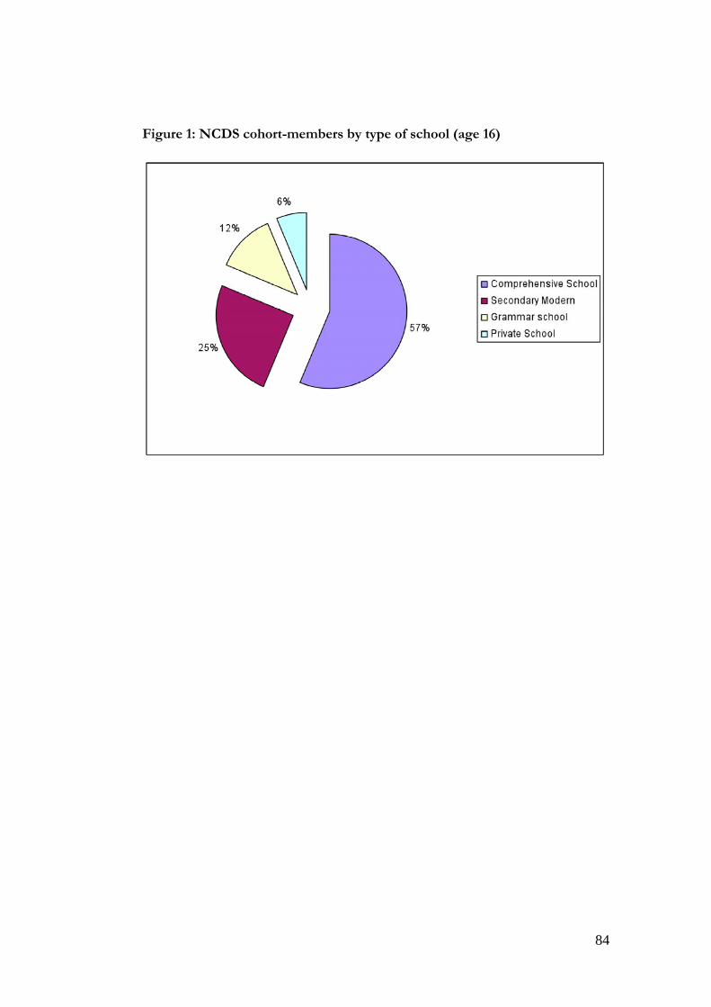
84

Figure 1: NCDS cohort-members by type of school (age 16)

85

Figure 2: Distribution of pupil-teacher ratios by type of primary school

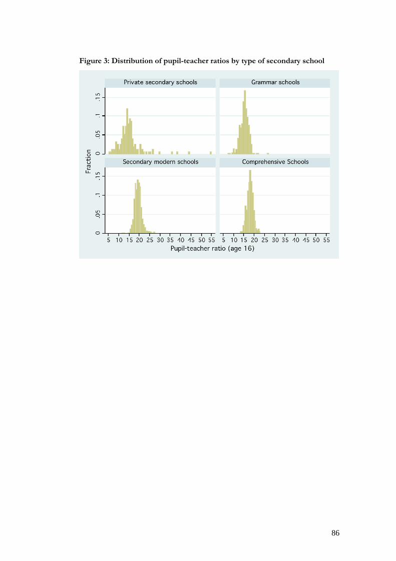
86

Figure 3: Distribution of pupil-teacher ratios by type of secondary school

87

Figure 4: Distribution of cognitive and non-cognitive ability in the NCDS cohort

88

Figure 5: Stochastic dominance: empirical distributions of SAH (age 46) by

type of secondary school

89

Figure 6: Stochastic dominance: empirical distributions of mental illness

(age 46) by type of secondary school

90

Chapter 5

The Impact of Childhood Cognitive Skills, Social Adjustment and Schooling on Adult Health and Lifestyle

5.1 Introduction The association between educational attainment and a range of health outcomes is

well documented in the economic literature, as reviewed by Grossman (2006) and

Cutler and Lleras-Muney (2008). Studies such as Currie and Moretti (2003), Lleras-

Muney (2005), Arendt (2005), Lindeboom et al. (2009), Kenkel et al. (2006),

Oreopoulous (2006), Grimard and Parent (2007), and Webbink et al. (2010)

additionally find evidence to suggest that part of this relationship may be causal.

Mazumder (2008) and Cutler and Lleras-Muney (2008, 2010) outline some of the

channels through which education may have an impact on health and health-related

behaviours: these include the effect of education on employment, both the type of

jobs available to people and their lifetime earnings; the effect on relative social

status; and the effect on use of health care and other health-related behaviours,

through the acquisition of specific health knowledge, through improved

information processing and decision-making skills, and through the influence on

behavioural responses to future costs and benefits and to perceived health risks.

Another recent strand of papers, such as Trannoy et al. (2009) and Rosa Dias

(2009), suggests that, in addition to family background, differences in education

may be a leading cause of inequality of opportunity in health. Less is known,

however, about whether quality of schooling also has an impact on health and how

this interacts with the effect of educational attainment45.

The National Child Development Study (NCDS) follows a cohort of

around 17,000 individuals, who were born in the week of 3rd March 1958, from

birth up until age 46. Members of the cohort were aged 11 in March 1969. They

went through secondary schooling during the 1970s and attended very different

types of school. The cohort’s secondary schooling lie within the transition period of 45 This gap in the literature is acknowledged in Cutler and Lleras-Muney (2008: p. 22).

91

the comprehensive education reform that was implemented in England and Wales

from the mid-1960s46. This was a major reform, aimed at reducing inequality of

opportunity, which transformed secondary education. Comprehensive schooling

was not implemented simultaneously nationwide, hence some of the cohort

members attended the highly selective tri-partite system of state-funded education,

which comprised grammar schools, secondary modern schools and a dwindling

number of technical schools. Among members of the NCDS cohort, 12 per cent

attended grammar schools at age 16, 25 per cent attended secondary moderns and

57 per cent attended comprehensives. A further 6 per cent of NCDS cohort

members attended private fee-paying schools, independent of the state educational

system and reforms47.

This paper is concerned with evaluating the impact of educational

attainment and of attending qualitatively different types of school on health

outcomes and health-related behaviour later in life. It contrasts the health outcomes

of the NCDS cohort members who experienced the selective system with those

who experienced the comprehensive system of education. This is in line with the

strategy of using major educational policy reforms to identify causal effects of

education on health. Similar identification strategies have been used in the recent

literature, often focusing on changes in the minimum school leaving age and related

reforms (see e.g., Lleras-Muney, 2005; Arendt, 2005, 2008; Oreopoulos, 2006;

Albouy and Lequien, 2008; Mazumder, 2008; Silles, 2009; Van Kippersluis et al.,

2009; Chou et al., 2010).

The comprehensive education reform was aimed at reducing inequality of

opportunity by improving the quality of schooling available to children from

disadvantaged backgrounds. These reforms have been evaluated in terms of their

direct impact on educational attainment and subsequent impact on labour market

outcomes (see e.g., Kerkchoff et al., 1996; Jesson, 2000; Dearden et al., 2002;

Galindo-Rueda and Vignoles, 2004, 2005; Pischke and Manning, 2006). Here we

46 Data on those who attended school in Scotland at age 16 are not used: the Scottish educational system of the 1960s and 1970s was structurally very different from the one experienced by the other NCDS cohort-members, and comprehensive schooling was introduced earlier, preventing a legitimate comparison of types of school, educational qualifications and outcomes. 47 Historically the leading private schools within the independent sector have been known as “public schools” in Britain. To avoid confusion we use the label “private schools” throughout. Most of our analysis focuses on those who went to state schools (grammar, secondary modern and comprehensive).

92

focus on a possible indirect consequence of the reform, by estimating the effect of

educational attainment and quality of schooling on adult health outcomes. We do

not evaluate the impact of comprehensive schooling per se but use the consequent

variation in quality of schooling and educational attainment as a natural experiment

to explore the impact on health and health-related behaviour.

We use a matching framework to pre-process the data: using a combination

of coarsened exact matching along with propensity score and Mahalanobis

matching (Ho et al., 2007). This is important because our own descriptive analysis,

as well as previous work with the NCDS, shows an imbalance between the

observed pre-schooling characteristics of those who attended comprehensive and

selective schools (Pischke and Manning, 2006). This is reinforced by regressions for

cognitive ability at age 7 and ‘value-added’ regressions of ability at age 11, given

ability at age 7, of the type used by Pischke and Manning (2006). First we use

matching to improve the balance of a broad set of observed pre-schooling

characteristics, including cognitive ability measured at age 7, between those who

attended comprehensive schools and a control group who attended selective state

schools. Then, to explore heterogeneity in the impact of attainment, those who

attended grammar schools are matched with a comparable group who attended

comprehensive schools and, likewise, those who went to secondary modern schools

are matched with a comparable group from comprehensive schools. A key

matching variable is ability at age 11, which is closely linked to likely performance in

the ‘Eleven Plus’ entry examination. But, rather than using absolute cognitive ability

at age 11, which is likely to be contaminated by a form of post-treatment bias due to

the ‘coaching effect’ for those who actually faced the Eleven Plus examination, we

use the relative ability ranking of those within the selective and non-selective

systems. The success of our matching strategy is assessed using value-added

regressions and other diagnostics.

The use of matched samples is coupled with parametric modelling of health

outcomes and health-related behaviour, using regression and instrumental variables

(IV) estimators. Our study design is structured to answer the following research

questions:

• On average, what is the overall impact of educational attainment, captured

by a detailed measure of the highest qualification attained, and of the quality

93

of schooling on adult health and health-related behaviour? This comparison

uses matching to balance the sample and controls for an extensive set of

observed pre-schooling characteristics using linear and nonlinear regression

methods.

• How do the estimated impacts of attainment and quality of schooling differ

when we take account of unobserved factors? This is addressed by adopting

an IV strategy, based on geographic variation in implementation of the new

policy and in the availability of comprehensive school places, that has been

used in earlier work.

• The key feature of the pre-comprehensive system was the distinction

between attending grammar and secondary modern schools: is there

heterogeneity in the impact of educational attainment, particularly according

to the type of school attended? This is explored by creating matched

samples, linking those who actually went to grammar or secondary modern

schools with comparable counterparts who went to comprehensive schools

and then applying parametric models to these matched sub-samples.

Our results show that cognitive ability at age 7 is not significantly associated

with health outcomes but there is a strong association with non-cognitive skills, as

reflected by social adjustment as a child. Those who had problems with social

adjustment are more likely to suffer both physical and mental illness as adults.

There is also evidence of a socioeconomic gradient in illness by father’s social class.

Those with poorer social adjustment as children are more likely to become smokers

and those whose father came from the higher or middle social classes are less likely

to become smokers. When those who went to grammar and to secondary modern

schools are matched separately to comparable groups who attended

comprehensives there is evidence of heterogeneity in the impact of educational

attainment, as measured by qualifications. Attainment has an impact on adult

health-related behaviours for both groups, in particular on smoking, drinking and

diet. But attainment only has an impact on adult health, both long-standing illness

and mental health problems, for those who either did or would have attended

grammar schools.

94

5.2 Comprehensive schooling reforms and the 1958 cohort The comprehensive education reform, put into place during the 1960s and 1970s in

England and Wales, replaced the selective educational system with a non-selective,

comprehensive system of secondary schooling. This policy reform was

implemented at different speeds at the local level: some local education authorities

(LEAs) implemented it quickly, but others resisted the change, some for decades.

Because of this slow and uneven transition, the two systems co-existed for a long

period of time and approximately 40 per cent of the NCDS cohort, who entered

state secondary schools in 1969, experienced the pre-reform selective system; the

remaining 60 per cent attended comprehensive schools.

Grammar schools were academically oriented state schools that provided

teaching for the entire age range 11-18, including a sixth form for Advanced level

(‘A-level’) studies, and prepared pupils to go on to higher education. Admission into

these schools was determined by an exam taken at age 11 (the ‘Eleven Plus’)48.

Pupils whose examination score did not permit entry into a grammar school

attended either secondary modern schools, which were less academically oriented

and covered the ages 11-16 or, in a small minority of cases, vocational schools

aimed at providing training and technical apprenticeships49.

The different types of schools varied in their curricula, examinations and

academic environment, along with other qualitative differences. Table 1 shows that,

among the schools attended by the NCDS cohort members used in our analysis at

age 16, 79 per cent of private schools and 69 per cent of grammar schools were

single sex, while only 13 per cent of comprehensive schools were single sex.

Streaming of classes by academic ability was common in secondary modern schools

(42 per cent) and comprehensive schools (39 per cent) but rare among grammar

schools (17 per cent). Some comprehensive schools were former secondary

moderns (26 per cent) or grammar schools (19 per cent), with the rest being newly

created.

48 Following much controversy, the selective system went into decline in the 1960s and 1970s, until the Eleven Plus was abolished as a national examination in England and Wales by the 1976 Education Act. Despite this, the selective system and the existence of grammar schools has persisted in certain areas, such as Kent. 49 In a few cases, pupils whose CSE grades were sufficient transferred to grammar schools or sixth form colleges to complete their A-levels.

95

Table 1 Characteristics of different types of schools (as attended by NCDS cohort at age 16)

Grammar Sec Modern Comprehensive Private % single sex 68.7 26.1 13.8 78.9 % with ability streams

16.6 42.3 38.8 22.8

% former grammar

- - 19.0 -

% former sec modern

- - 26.3 -

Note: The percentages are computed using all available observations for the relevant variables. The comprehensive reform has received considerable attention in the

literature and its impact on educational outcomes has been assessed. The evidence

for the impact on educational outcomes is mixed. Kerckhoff et al. (1996) review a

series of LEA case studies and use NCDS data to examine the association between

types of secondary schools and exam performance at age 18. After controlling for a

wide range of observables, including measures of cognitive ability prior to

secondary education, the authors find no association between the average academic

achievements of pupils in selective and in comprehensive schools. However, when

the impact of the reform is examined for different quantiles of ability, the study

finds that high-ability pupils performed relatively worse and low-ability pupils

performed relatively better in comprehensive schools. Jesson (2000) implements a

value-added approach that corroborates most of these results. Accounting for a rich

set of controls, the paper finds no significant differences between the exam

performance of pupils in the selective and comprehensive systems of education.

Nevertheless, pupils in secondary modern schools performed worse in exams than

their comprehensive school counterparts.

Galindo-Rueda and Vignoles (2004) investigate the causal effects of the

comprehensive reform on educational outcomes; the data used are from the NCDS

and their research strategy is based on matching and instrumental variables

estimators. Two instruments are used for type of schooling: Conservative Party

control of the cohort members’ LEA (which the authors claim to be negatively

correlated with the probability of attending a comprehensive school, but orthogonal

96

to the educational outcomes) and the share of comprehensive schools in a cohort-

member’s LEA. Although point estimates of the policy impact are shown to be

sensitive to the choice of instrument, the results suggest that the most able 20 per

cent of pupils did relatively better in the selective school system than they would

have done in a comprehensive one; no statistically significant effect of the reform

was found for pupils in the lower ability quantiles. Maurin and MacNelly (2007) add

to this body of evidence by evaluating a different school reform, implemented in

Northern Ireland in the late 1980s. The educational system in Northern Ireland

remained selective, with the policy reform designed to increase the number of

pupils allowed to attend a grammar school by 15%. The paper compares the

educational outcomes between Northern Ireland and England before and after the

reform (using the English comprehensive education system as a control group); the

wider access to grammar schools within the Northern Irish selective system is

found to have a large positive impact on educational attainment.

Pischke and Manning (2006) have raised a fundamental challenge to this

literature. They also use NCDS data but they question the main results of earlier

work. First, contrary to Kerckhoff et al. (1996), they find that comprehensive areas

were systematically poorer and populated by children with lower ability than

selective areas. The policy impacts reported in the literature may thus be the result

of selection bias. Second, using a series of placebo tests based on value-added

regression for ability, they find that the comparison between areas exposed to

different degrees of educational selectivity tend to produce the same results

regardless of whether the educational outcomes are measured after the reform or

before it. We draw on Pischke and Manning’s (2006) placebo tests to assess whether

our empirical strategy achieves the goal of making valid inferences about the impact

of educational attainment and of quality of schooling.

5.3 NCDS data and study design Members of the National Child Development Study (NCDS) cohort were all born

in the week of 3rd March 1958. Seven waves of interviews have been carried-out

when cohort members were 7, 11, 16, 23, 33, 42 and 46 years old. The study

compiles detailed information on the cohort-members’ childhood health, parental

background, and educational achievement. It also includes self-reported

97

information on social status in adulthood, health-related behaviour and a wide range

of health outcomes. The NCDS gathers data from a variety of sources. In the early

waves this includes information from parents, medical examinations, tests of ability

and from the child’s school. In the later waves these are augmented by interviews

with the cohort members and data linked from the Census.

Fig. 1. Schematic view of study design and NCDS variables

Family SES• Father’s SES(3 groups)• {Mother & father’s years of schooling}• Financial hardship (age 7)• Region• ED characteristics

Family & childhood health• Gender• Morbidity index (age 7)• Hospitalisations (age 7)• {Obesity (age 16)}• {Maternal smoking} • Family illness (diabetes, epilepsy, heart disease)

Ability:Cognitive

•Tests at age 11 & age7Non-cognitive

• BSAG at age 11

Schooling• Primary school (size of class at 7, unhappy, parents’ plans)• School type (age 16)• School characteristics• Qualifications

Adult lifestyle• Smoking (age 33, 42 & 46)• Drinking (age 42)• Vegetables (age 33)• Fried food (age 33)• Smoking during pregnancy

Adult health • Long-standing illness (age 46)• Malaise (age 42)

Note: Items in braces are not used in our main analysis but are used in the checks for robustness.

The structure of the NCDS is well-suited to our study design, which is

summarised in Figure 1. Our goal is to identify the impact of educational attainment

and of the characteristics of secondary schooling experienced by members of the

1958 cohort on outcomes later in life, with a focus on health-related behaviour and

adult health. The NCDS allows us to condition on a broad set of pre-treatment

factors that reflect early life circumstances, occur prior to secondary schooling, and

are not influenced by subsequent educational choices (Dearden et al., 2002). These

factors fall into three broad groups: measures of family socioeconomic status and

98

the local environment during early childhood; measures of childhood health and use

of health care and health within the family; and measures of cognitive and non-

cognitive skills and social adjustment of the child. In addition we condition on

characteristics of the individual’s primary education. The aim is to estimate the

impact of the type and characteristics of the secondary schooling experienced by

each individual on their adult outcomes, both the intermediate outcomes, such as

smoking at age 42, and final health outcome, such as long-standing illness at age 46.

The specific variables that are available within each of the broad categories are

described below and are listed in full in Table A.1 (Appendix D).

5.3.1 Childhood health and parental background

Rich information is available to characterise the cohort members’ childhood health

and parental circumstances, which have both been linked to adult health outcomes

(see e.g., Case et al., 2005; Currie and Stabile, 2004). Following Power and Peckham

(1987), indicators of morbidity are constructed by aggregating twelve categories of

health conditions, that affect the child at ages 7 and 11. Dummy variables for the

occurrence of diabetes, epilepsy and other chronic conditions among parents and

siblings are included in order to account for the incidence of hereditary conditions

in the cohort member’s family. Information on obesity at age 16 is also available, as

well as an indicator variable for maternal smoking after the fourth month of

pregnancy.

In terms of parental background, the NCDS allows us to trace the social class

and the years of schooling of the parents of cohort members. We use the father’s

occupational socioeconomic status (SES), measured in three groups (see Carneiro et

al., 2007). Following Case et al. (2005) and Lindeboom et al. (2009), this information

is complemented by data on the incidence of household financial difficulties during

the cohort member’s childhood and adolescence.

5.3.2 Cognitive ability, non-cognitive skills and social adjustment

Auld and Sidhu (2005) argue that failure to control for cognitive ability will

confound the relationship between health and education. Non-cognitive skills have

99

also received considerable attention in recent studies (see for example, Heckman et

al., 2006; Heckman, 2008) and have been linked to health and health-related

behaviours (see e.g., Carneiro et al., 2007; Coneus and Laucht, 2008; Cutler and

Lleras-Muney, 2010; Keaster, 2009). Among these non-cognitive skills, social

adjustment is of particular relevance for schooling and health (Carneiro et al., 2007).

The NCDS provides measures of cognitive and non-cognitive ability

collected before respondents began their secondary schooling. Scores of ability

tests taken at age 7 and 11 are available on a series of cognitive dimensions:

mathematics, reading, copying designs and general ability. These test scores are

highly correlated at the individual level leading to problems with precision in

econometric models, due to multicollinearity. To avoid this, we follow Galindo-

Rueda and Vignoles (2005) and use principal components analysis to construct a

single measure of cognitive ability using the first principal component50. The

empirical distributions of these combined scores, for the tests at ages 7 and 11, split

by type of secondary school attended at age 16 are presented in Figure 2.

The similarity of the distribution of scores between the two ages and the

pattern across schools provides confidence in their face validity: ability scores are

lowest among those who attended secondary moderns, followed by those who

attended comprehensives. The distributions for grammar and private schools are

similar, but with more children in both the lower and upper tails among private

school pupils.

It should be emphasised that the three dimensions of cognitive ability used

to construct our index – mathematics, reading and general ability – along with the

fact that the index derived from the first principal component gives equal weight to

each dimension, mirrors the three elements of the Eleven Plus examination. So the

cognitive ability score at age 11 can be viewed as a proxy for performance in the

Eleven Plus for those who took the examination.

50 For example, with the scores at age 11, the first principal component accounts for 85 per cent of the joint variation and, strikingly, the weights attached to the three dimensions – 0.583, 0.567 and 0.582 – are virtually identical.

100

Fig. 2. Empirical distributions of cognitive ability scores by type of school

(a) Age 7 scores

(b) Age 11 scores

Following Carneiro et al. (2007) the score for the Bristol Social Adjustment

Guide (BSAG) is used as a measure of social skills. This is a measure of problems

with social adjustment at age 11: teachers were asked to report whether the child

had problems in twelve behavioural domains such as hostility towards children and

adults, anxiety, withdrawal, ‘writing off’ adults, unforthcomingness, depression,

restlessness, acceptance by adults, inconsequential behaviour, as well as

miscellaneous psychological and nervous symptoms (Stott, 1987). One point is

101

attributed to each positive answer; points are then summed to obtain the BSAG

social maladjustment score51. The distribution of the BSAG measure is presented in

Figure 3, which shows that the distribution is highly skewed with relatively few

respondents having high scores for social maladjustment.

Fig. 3. Empirical density of Bristol Social Adjustment Guide (BSAG)

Note: The Figure shows the histogram of the BSAG score,

a kernel density estimate and a normal curve.

5.3.3 Local area characteristics

The NCDS includes information about the area in which the cohort-members lived,

aggregated at different geographic levels. Data on the cohort members’ UK

standard region is available for all the waves of the study. For the years 1971 and

1981, NCDS survey data was linked to the Census, allowing a detailed demographic

and socioeconomic characterisation of each individual’s local area, at the electoral

constituency level, local education authority level and census enumeration district

level (the smallest unit for which census statistics were then available, with an

average population of about 460) 52. Measures include the percentage of the local

51 The NCDS data dictionary notes that that this the scores “are added together to give a figure which indicates, fairly crudely, the total amount of behavioural deviance (maladjustment) as measured by the Guide”. 52 This small area data are available under a special licence, which imposes restrictions on the handling and usage of the data. Details can be found at: http://www.cls.ioe.ac.uk/studies.asp?section=0001000200030015.

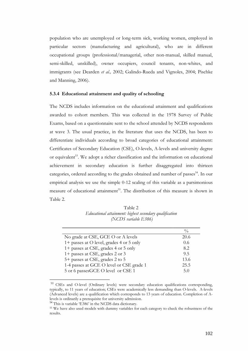
102

population who are unemployed or long-term sick, working women, employed in

particular sectors (manufacturing and agricultural), who are in different

occupational groups (professional/managerial, other non-manual, skilled manual,

semi-skilled, unskilled), owner occupiers, council tenants, non-whites, and

immigrants (see Dearden et al., 2002; Galindo-Rueda and Vignoles, 2004; Pischke

and Manning, 2006).

5.3.4 Educational attainment and quality of schooling

The NCDS includes information on the educational attainment and qualifications

awarded to cohort members. This was collected in the 1978 Survey of Public

Exams, based on a questionnaire sent to the school attended by NCDS respondents

at wave 3. The usual practice, in the literature that uses the NCDS, has been to

differentiate individuals according to broad categories of educational attainment:

Certificates of Secondary Education (CSE), O-levels, A-levels and university degree

or equivalent53. We adopt a richer classification and the information on educational

achievement in secondary education is further disaggregated into thirteen

categories, ordered according to the grades obtained and number of passes54. In our

empirical analysis we use the simple 0-12 scaling of this variable as a parsimonious

measure of educational attainment55. The distribution of this measure is shown in

Table 2.

Table 2 Educational attainment: highest secondary qualification

(NCDS variable E386)

% No grade at CSE, GCE O or A levels 20.6 1+ passes at O level, grades 4 or 5 only 0.6 1+ passes at CSE, grades 4 or 5 only 8.2 1+ passes at CSE, grades 2 or 3 9.5 5+ passes at CSE, grades 2 to 5 13.6 1-4 passes at GCE O level or CSE grade 1 25.5 5 or 6 passesGCE O level or CSE 1 5.0

53 CSEs and O-level (Ordinary levels) were secondary education qualifications corresponding, typically, to 11 years of education; CSEs were academically less demanding than O-levels. A-levels (Advanced levels) are a qualification which corresponds to 13 years of education. Completion of A-levels is ordinarily a prerequisite for university admission. 54 This is variable ‘E386’ in the NCDS data dictionary. 55 We have also used models with dummy variables for each category to check the robustness of the results.

103

7+ passes at GCE O level grades A-C, or CSE grade 1 3.5 1 pass at A level, grades A-E 2.9 2 passes at A levels, up to 8pts 3.7 3+ passes at A levels, up to 8pts 2.7 2 passes at A levels and 9+ pts 0.2 3+ passes at A levels and 9+pts 4.0 N=11,086

Note: A level points are allocated as 5, 4, 3, 2 and 1 for grades A-E

respectively.

Our analysis of the impact of secondary schooling controls for information

about the individual’s experience in primary school as well as their parents’

educational aspirations for their child (see Dearden et al., 2002). This includes the

number of children in the child’s primary school class at age 7 in 1965, whether

parents reported that their child was unhappy at school in 1965, and an indicator of

the parents’ aspirations for the child, indicating whether they wished the child to

continue beyond the minimum school leaving age.

Type of secondary schooling is captured by indicators of the school

attended at age 16 (in 1974): secondary modern, grammar, comprehensive or

private. This classification is augmented by information on the characteristics of the

school, including the teacher/pupil ratio, the ratio of expelled pupils to the total

number, and indicators of whether the school was single sex and whether classes

were streamed by ability (see Dearden et al., 2002). It is these measures that are used

to capture quality of schooling in the regression models56.

Geographic variation in the availability of comprehensive schooling

provides the instruments used in the IV strategy. These variables are described in

more detail below, but they include the percentage of the LEA that was

comprehensive in 1974 and a measure of local political affiliation based on

Conservative party control of electoral constituencies (as used by Galindo-Rueda

and Vignoles, 2004).

5.3.5 Intermediate outcomes: health-related behaviours

56 The literature on the impact of school resources, as reflected in the pupil-teacher ratio, on educational attainment in the NCDS provides mixed results (Feinstein and Symons, 1999; Dearden et al., 2002; Dustmann et al., 2003).

104

The NCDS contains self-reported information on a series of health-related

behaviours which may be influenced by schooling and go on to affect adult health.

The survey includes data on the number of cigarettes smoked per day, average units

of alcohol consumed per week57 and dietary choices, such as the frequency of

consumption of fried food and vegetables. These data are only available in the latter

four waves of the study, once respondents are aged 23 and above. The other

measure of health-related behaviour relates only to the women in the cohort: an

indicator for whether mothers, of any age up to 42, smoked during their

pregnancies.

A particular focus is on smoking which is the largest cause of avoidable

premature death in the UK. We have information on smoking at each of the waves

4-7, spanning ages 23 to 46. As there is item non-response at each wave using a

combined measure leads to loss of sample size, so we have decided to focus on

smoking at age 42 (wave 6). The prevalence of smoking at age 42 is 25 per cent. Of

those with available data on smoking for waves 5-7 (ages 33, 42 and 46) 69 per cent

never smoked. Among those who smoked at some point, 74 per cent reported

smoking at age 42. The remainder are mostly those who had smoked at age 33 but

not at 42 or 4658. So our measure captures those whose damaging health-related

behaviour persists into their mid-forties.

5.3.6 Main outcomes: adult health

Our principal measure of health in adulthood is self-reported long-standing illness

or disability at age 46. Information on the particular medical condition associated

with the long-standing illness is available and classified according to the

International Classification of Diseases (ICD-10). Table 3 shows that the

conditions most often listed as the source of the long-standing illness are problems

with the musculoskeletal system (25.7 per cent), circulatory system (11.8 per cent),

57 NCDS respondents are asked about their weekly consumption of a wide range of alcoholic drinks (glasses of wine, pints of beer and so forth). These are then converted to units of alcohol using the UK National Health Service official guidelines that are available at: http://www.nhsdirect.nhs.uk/magazine/interactive/drinking/index.aspx . 58 To check robustness all of our analyses were repeated with an indicator of smoking in any of the waves 5-7. The prevalence of smoking in any of these waves is 30 per cent. Results for these analyses are not presented here. The sample sizes are smaller but otherwise results are comparable to the ones for smoking at wave 6. The same applies to using the prevalence of smoking at wave 7 rather than wave 6.

105

respiratory system (11.4 per cent) and metabolic problems (9.5 per cent), of which

70 per cent suffer from diabetes.

Mental health in adulthood is also taken into account as an outcome

through respondents’ answers to a series of questions from the Cornell Medical

Index Questionnaire, each targeting a particular mental ailment. The number of

positive answers given, at age 42, is then used as a malaise score along the lines of

Carneiro et al. (2007). The malaise score is a measure of psychiatric morbidity (with

a special focus on depression), developed at the Institute of Psychiatry from the

Cornell Medical Index ( Rutter et al., 1970). The NCDS team suggest the use of a

severity scale: individuals are considered normal if they score between 0 and 7

points and depressed if they score between 8 and 24 points (Rodgers et al., 1999)59.

In our data the malaise index, at age 42, ranges from 0 to 23, with a mean of 3.4.

Table 3 Breakdown of long-standing illness (LSI) by percentage with specific main

conditions (ICD-9)

Wave 7 (age 46)

Infectious & parasitic diseases 0.7 Neoplasms 1.6 Diseases of blood & immune mechanism 1.5 Endocrine, nutritional and metabolic 9.5 Mental and behavioural disorders 5.9 Nervous system 5.9 Eye, ear and mastoid process 4.6 Circulatory system 11.8 Respiratory system 11.4 Digestive system 5.5 Skin 2.1 Muscoloskeletal system 25.7 Genitourinary system 2.0 Congenital malformations 0.3 Undiagnosed illness 1.8 Injury, poisoning etc 5.3 Other LSI/uncoded 4.3 N=2990

59 Carneiro et al. (2007) define an indicator variable for depression based on this rule of thumb.

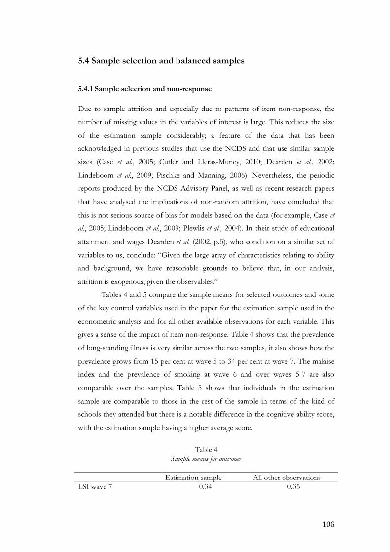
106

5.4 Sample selection and balanced samples

5.4.1 Sample selection and non-response

Due to sample attrition and especially due to patterns of item non-response, the

number of missing values in the variables of interest is large. This reduces the size

of the estimation sample considerably; a feature of the data that has been

acknowledged in previous studies that use the NCDS and that use similar sample

sizes (Case et al., 2005; Cutler and Lleras-Muney, 2010; Dearden et al., 2002;

Lindeboom et al., 2009; Pischke and Manning, 2006). Nevertheless, the periodic

reports produced by the NCDS Advisory Panel, as well as recent research papers

that have analysed the implications of non-random attrition, have concluded that

this is not serious source of bias for models based on the data (for example, Case et

al., 2005; Lindeboom et al., 2009; Plewlis et al., 2004). In their study of educational

attainment and wages Dearden et al. (2002, p.5), who condition on a similar set of

variables to us, conclude: “Given the large array of characteristics relating to ability

and background, we have reasonable grounds to believe that, in our analysis,

attrition is exogenous, given the observables.”

Tables 4 and 5 compare the sample means for selected outcomes and some

of the key control variables used in the paper for the estimation sample used in the

econometric analysis and for all other available observations for each variable. This

gives a sense of the impact of item non-response. Table 4 shows that the prevalence

of long-standing illness is very similar across the two samples, it also shows how the

prevalence grows from 15 per cent at wave 5 to 34 per cent at wave 7. The malaise

index and the prevalence of smoking at wave 6 and over waves 5-7 are also

comparable over the samples. Table 5 shows that individuals in the estimation

sample are comparable to those in the rest of the sample in terms of the kind of

schools they attended but there is a notable difference in the cognitive ability score,

with the estimation sample having a higher average score.

Table 4

Sample means for outcomes Estimation sample All other observations LSI wave 7 0.34 0.35

107

(n=2832) (n=4663) LSI wave 6 0.27

(n=2700) 0.29

(n=6159) LSI wave 5 0.15

(n=2593) 0.15

(n=6286) Malaise wave 6 3.35

(n=2689) 3.63

(n=6103) Smoker wave 6 0.21

(n=2698) 0.27

(n=6152) Smoker waves 5-7 0.28

(n=2377) 0.32

(n=3695)

Table 5

Sample means for type of schooling and cognitive ability Estimation sample All other observations Comprehensive 0.55 0.57 Secondary modern 0.24 0.25 Private school 0.06 0.07 Attainment 4.76 3.95 Single sex school 0.28 0.27 Ability streams 0.35 0.38 Pupil-teacher ratio 0.06 0.06 Expelled ratio 0.0003 0.0004 Cognitive ability age 7 0.25 -0.02

5.4.2 Balance of covariates between selective and non-selective schools

Pischke and Manning (2006) have drawn attention to the fact that there may be an

imbalance in the pre-schooling characteristics of the NCDS respondents who went

to selective versus non-selective schools. They find that comprehensive areas were

systematically poorer and populated by children with lower educational

achievement than selective areas. In this section we explore this imbalance and

adopt a matching approach to preprocess the data and improve balance.

One measure that is commonly used to assess the balance of the

distribution of covariates in a treated (x1) and a control group (x0), before and after

108

matching, is the percentage bias, or normalised difference in means (Rosenbaum

and Rubin, 1983; Lalonde, 1986)60: 1 0

1 0.100

( ( ) ( )x x

Var x Var x−

+ (1)

The first column of results in Table 6 shows the percentage bias measure

for the unmatched data in our estimation sample for some of the key pre-schooling

variables: cognitive ability at 7, the BSAG score, father’s social class and ill health at

age 7. These reveal fairly substantial imbalance between those who went to

comprehensive schools and those who went to selective state schools, with the

percentage bias being as high as -16.8 per cent for cognitive ability. It is notable that

the percentage bias is even greater, at -31 per cent, for cognitive ability at age 11.

The fact that the imbalance is greater for the score at age 11 than it is for age 7 is

explored below: in addition to the selection bias discussed by Pischke and Manning

(2006) there appears to be a ‘coaching effect’ - those in selective areas were more

likely to practice the kind of ability tests used in the NCDS as part of their

preparation for the Eleven Plus.

Table 6

Percentage bias (normalised difference in means between comprehensive and selective schools) before and after pruning and matching for key covariates

Unmatched Matched t-test (p value) Cognitive ability age 7 -16.8 -0.1 -0.02 (0.984) BSAG score 3.8 -0.9 -0.25 (0.799) Father’s social class high -12.3 0.7 0.19 (0.852) Father’s social class middle

11.6 2.5 0.70 (0.487)

Ill-health age 7 0.8 0.2 0.05 (0.964) Cognitive ability age 11 -31.0 -30.1 -8.30 (0.000) Note: Cognitive ability at age 11 is not used as a matching variable.

60 t-tests for the difference in means are often proposed as a way of checking for balancing. This approach is criticised by Ho et al. (2007) and Imbens and Wooldridge (2008): for example, “the critical misunderstood point is that balance is a characteristic of the observed sample, not some hypothetical population. The idea that hypothesis tests are useful for checking balance is therefore incorrect.” (Ho et al., 2007). They argue that this is compounded by the fact that pruning the sample affects the statistical power of the hypothesis tests and that it is therefore misleading to use tests, such as t-ratios for the difference in means, as a guide to the quality of matching. However this diagnostic is widely used and, for completeness, we do present t-ratios for the differences in means within the matched sample in the final column of Table 6 and subsequent tables.

109

As the balancing condition relates to the full empirical distribution, not just

the sample means, it is wise to check higher moments and cross-moments. Ho et al.

(2007) suggest that nonparametric density plots and quantile-quantile (QQ) plots

for each covariate and their interactions should be compared for the treated and

controls. Figure 4 shows the empirical QQ plots for cognitive ability at age 7 and

the BSAG score for the unmatched and matched samples. For the unmatched

sample the divergence between the distributions is most clear in the tails of the

distributions, especially for the upper tail of the distribution of the BSAG score.

Fig.4. Empirical QQ-plots for cognitive score at 7 and BSAG score:

Before (left panels) and after (right panels) matching

Perfect balancing is unlikely to be achieved in practice and, rather than

simply comparing means after matching, running parametric regression models on

the matched sample is likely to improve causal inferences (see e.g., Rubin, 1973,

1979, 2006; Heckman, Ichimura and Todd, 1998; Imbens, 2004; Abadie and

Imbens, 2006; Ho et al., 2007). In this sense, matching can be used as a

nonparametric preprocessing of the data to select observations prior to parametric

modelling. We adopt this approach here.

We implement the matching in two steps. In the first step coarsened exact

matching is applied to the key measures of cognitive and non-cognitive skills, the

110

ability score at age 7 and the BSAG score at age 1161. Then any observations that lie

outside the common support of their joint distribution are excluded: this is only 34

cases in our data. The second step uses a combination of propensity score and

Mahalanobis exact matching. The propensity score for attending a comprehensive

school, as a function of all of the pre-schooling variables, is estimated using a logit

model. The propensity score controls for the main pre-policy potential confounders

of the relationship between attendance at a particular type of school and the health

outcomes of interest. Figure 5 shows the distribution of the propensity score

among those who went to selective and to comprehensive schools. Those who went

to comprehensive schools are then matched with those who went to selective

schools using the propensity score, within the common support and with a caliper

of 0.1, combined with exact Mahalanobis matching for two key covariates, cognitive

ability at age 7 and the BSAG score. The matching weights are then used in the

subsequent regression analyses.

The normalised differences and t-ratios shown in Table 6 and the QQ plots

in Figure 4 show how the imbalance in the key covariates is largely removed by this

matching process. Table 6 also includes the cognitive ability scores at age 11, which

are not used in the matching process. The percentage bias remains substantial for

this variable (30.1 per cent) in the matched data. This is explored in the next

section.

61 Coarsened exact matching works by splitting the support of continuous covariates into discrete intervals and computing cell frequencies for the multivariate histogram (Blackwell et al., 2009).

111

Fig.5. Distribution of propensity score over selective (“untreated”) and non-selective (“treated”) schools

5.4.3 ‘Coaching effects’: absolute and relative cognitive ability

Cognitive ability at age 11 is not used in the matching process because there are

good reasons to suspect that matching on the score at age 11 may be a source of

post-treatment bias62. Those children who lived in areas which had not gone

comprehensive may have been exposed to ‘coaching’ to prepare them for the

Eleven Plus, both within their primary schools, where time was often set aside in

lessons to prepare for the test, and at home. The cognitive ability test, also

administered at age 11, have a lot in common with the components of the Eleven

Plus and the resulting scores may therefore be indirectly affected by the kind of

secondary school the child was likely to attend. In the matching approach described

above we avoid this post-treatment bias by matching on ability at age 7.

Another way of looking at the issue is to focus on relative ability. Figure 6

shows the empirical distributions for relative ability, where rank in the distribution

of ability is computed separately for those who went to comprehensive schools and

who went to selective schools. By construction the distribution is uniform among

the group who went to comprehensive schools, but among those who went to

62 In fact, in our checks for robustness, we have repeated the matching and regression analyses using absolute ability. This shows that the qualitative estimates of the impact of educational attainment and type of schooling are robust to using either absolute or relative measures and that changes in the magnitudes of the estimates are small.

112

selective schools there is a clear threshold, around the lower 60 per cent of ability

scores between those who went to secondary moderns and those who went to

grammar schools. Relative ability therefore plays a central role in creating matched

samples by type of school.

Fig.6. Empirical distributions of relative ability by type of school

This coaching effect is one way of explaining the results presented by

Pischke and Manning (2006) and this is now explored in more detail. First we

estimate simple regressions for cognitive ability at age 7 (Score7), conditioning on an

indicator of attending a comprehensive school (Comp) and the other pre-schooling

characteristics. The coefficient on Comp indicates any selection bias due to

systematic differences between those who attended selective versus comprehensive

schools, over and above the pre-schooling variables included in the equation, that

influence cognitive ability. Table 7 shows that there is a statistically significant

difference in the raw data but this disappears when the matched sample is used. The

second regression is a value-added specification that regresses cognitive ability at

age 11 on ability at age 7, the indicator for comprehensive schooling and an

interaction between the two, as well as the other pre-schooling characteristics.

Lagged ability captures any selection that has occurred up to age 7 as well as the

inherent persistence in cognitive ability, the coefficient on Comp is now interpreted

as capturing the ‘coaching effect’ and the coefficient on the interaction term

captures any difference in the value-added between those who went on to become

113

comprehensive pupils and others. The coaching effect is large and statistically

significant but we do not find evidence of a statistically significant interaction effect

for either the unmatched or matched data.

Table 7 Regressions for cognitive ability scores at ages 7 and 11: full sample

Score

Unmatched age 7

Matched Score

Unmatched age 11

Matched Comp -0.143

(-3.43) -0.020 (-0.36)

-0.252 (-5.79)

-0.438 (-7.58)

Score7

- - 0.785 (27.04)

0.732 (13.98)

Score7*comp

- - -0.028 (-0.78)

0.014 (0.25)

R2 0.135 0.147 0.514 0.493 Sample size 2657 2211 2657 2211 Notes:

i. All regressions also condition on the full set of pre-schooling covariates. See Table A.1 for a full list.

ii. Robust t-ratios are given in parentheses. Coefficients that are statistically significant at least a 10 per cent level are shown in bold.

5.4.4 Matched sub-samples

The impact of educational attainment and quality of schooling is likely to depend

on the particular type of school that is attended. The existence of heterogeneous

effects is explored using a further round of matching that exploits the natural

dividing in the population line drawn by the reform: the one separating those who

experienced, or would have experienced in the absence of the reform, a grammar

school education and those who attended, or would have attended, secondary

modern schools. The matching is based on the propensity score for the probability

of attending a grammar versus a secondary modern school. This is estimated by a

logit model using only the sample who attended selective schools. Predictions of the

propensity score are then computed for the whole sample, including those who

attended comprehensive schools. The key predictor, that dominates the predictions

from the logit model, is relative ability at age 11 (as shown in Figure 6). Those who

were exposed to the non-selective system but whose propensity score indicates that

114

they would have attended a grammar school (secondary modern) were they not

exposed to the reform, are then matched with those who actually attended at a

grammar school (secondary modern). The matching is over the common support

with a caliper of 0.1 and uses Mahalanobis matching on the propensity score and

exact matching on relative ability at age 11, absolute ability at age 7, the BSAG score

and father’s social class. Tables 8 and 9 compare the balancing of selected covariates

before and after matching for the two sub-samples and demonstrate that a good

balance is achieved for both. The final rows of the table show that balance in terms

of relative ability at age 11 does not imply balancing of absolute ability63.

Table 8 Percentage bias (normalised difference in means between grammar and comprehensive schools) before

and after matching for key covariates: sub-sample of grammar and comprehensive pupils Unmatched

sample Matched sample t-ratio (p value)

Relative ability age 11 107.3 2.1 0.43 (0.670) Cognitive ability age 7 93.2 1.8 0.35 (0.724) BSAG score -44.7 3.1 0.57 (0.569) Father’s social class high

47.4 0.0 0.00 (1.000)

Father’s social class middle

-31.9 0.0 -0.00 (1.000)

Ill-health age 7 -15.0 9.2 1.43 (0.152) Cognitive ability age 11 144.6 41.5 8.37 (0.000) Note: Cognitive ability at age 11 is not used as a matching variable.

Table 9 Percentage bias (normalised difference in means between secondary modern and comprehensive

schools) before and after matching for key covariates: sub-sample of secondary modern and comprehensive pupils

Unmatched

sample Matched sample t-ratio (p value)

Relative ability age 11 -66.3 -2.4 -0.51 (0.613) Cognitive ability age 7 -25.4 -0.8 -0.16 (0.873) BSAG score 21.1 3.2 0.55 (0.582) Father’s social class -13.6 0.0 0.00 (1.000) 63 This is to avoid the potential for post-treatment bias. We have done robustness checks that include an analysis of what happens when relative ability is replaced by absolute ability.

115

high Father’s social class middle

1.7 0.0 0.00 (1.000)

Ill-health age 7 9.2 1.7 0.31 (0.760) Cognitive ability age 11 -28.8 31.4 6.54 (0.000) Note: Cognitive ability at age 11 is not used as a matching variable.

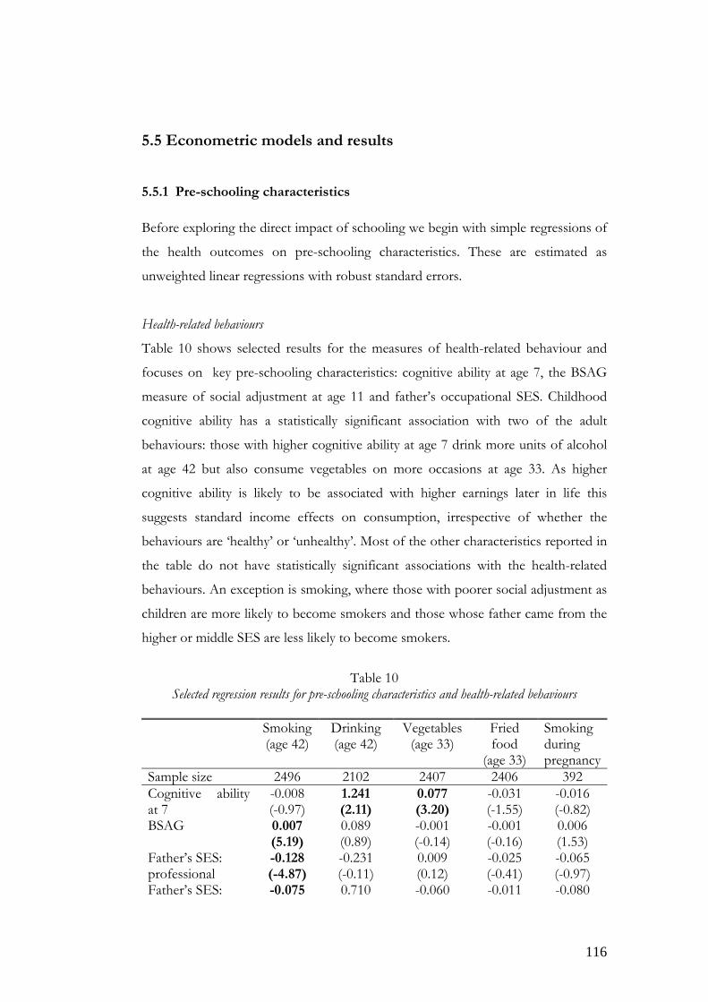
116

5.5 Econometric models and results

5.5.1 Pre-schooling characteristics

Before exploring the direct impact of schooling we begin with simple regressions of

the health outcomes on pre-schooling characteristics. These are estimated as

unweighted linear regressions with robust standard errors.

Health-related behaviours

Table 10 shows selected results for the measures of health-related behaviour and

focuses on key pre-schooling characteristics: cognitive ability at age 7, the BSAG

measure of social adjustment at age 11 and father’s occupational SES. Childhood

cognitive ability has a statistically significant association with two of the adult

behaviours: those with higher cognitive ability at age 7 drink more units of alcohol

at age 42 but also consume vegetables on more occasions at age 33. As higher

cognitive ability is likely to be associated with higher earnings later in life this

suggests standard income effects on consumption, irrespective of whether the

behaviours are ‘healthy’ or ‘unhealthy’. Most of the other characteristics reported in

the table do not have statistically significant associations with the health-related

behaviours. An exception is smoking, where those with poorer social adjustment as

children are more likely to become smokers and those whose father came from the

higher or middle SES are less likely to become smokers.

Table 10

Selected regression results for pre-schooling characteristics and health-related behaviours

Smoking (age 42)

Drinking (age 42)

Vegetables (age 33)

Fried food

(age 33)

Smoking during pregnancy

Sample size 2496 2102 2407 2406 392 Cognitive ability at 7

-0.008 (-0.97)

1.241 (2.11)

0.077 (3.20)

-0.031 (-1.55)

-0.016 (-0.82)

BSAG 0.007 (5.19)

0.089 (0.89)

-0.001 (-0.14)

-0.001 (-0.16)

0.006 (1.53)

Father’s SES: professional

-0.128 (-4.87)

-0.231 (-0.11)

0.009 (0.12)

-0.025 (-0.41)

-0.065 (-0.97)

Father’s SES: -0.075 0.710 -0.060 -0.011 -0.080

117

other non-manual (-3.00) (0.37) (-0.89) (-0.20) (-1.27)

Notes: i. The regression estimates are based on the un-weighted sample. ii. Robust t-ratios are given in parentheses. Coefficients that are statistically

significant at least a 10 per cent level are shown in bold. iii. All regressions also condition on the full set of pre-schooling covariates. See

Table A.1 (Appendix D) for a full list.

Health outcomes

Table 11 shows selected results for the health outcomes: long-standing illness at age

46 and malaise at age 4264. Cognitive ability is not significantly associated with

health outcomes but there is a strong association with social adjustment. Those with

more problems with social adjustment as children are more likely to suffer both

physical and mental illness as adults. There is also evidence of a socioeconomic

gradient in illness by father’s social class.

Table 11 Selected regression results for pre-schooling characteristics and health outcomes

LSI

LPM

Probit Malaise

Sample size 2623 2487 Cognitive ability at age 7 -0.008

(-0.87) -0.008 (-0.85)

-0.062 (-0.89)

BSAG score 0.005 (3.65)

0.005 (3.74)

0.050 (4.11)

Father’s SES: professional -0.036 (-1.23)

-0.035 (-1.22)

-0.376 (-1.78)

Father’s SES: other non-manual

-0.044 -0.043 -0.076

(-1.70) (-1.71) (-0.40)

See notes for Table 10.

64 The results show estimates for both a linear regression (linear probability) model and partial effects from a probit model, estimated at the mean of the regressors, for long-standing illness. The two specifications give virtually identical results and are presented to illustrate this finding. This applies to all of the nonlinear regression models we estimated and the rest of the paper focuses on linear regression results.

118

5.5.2 The impact of attainment and quality of schooling with controls for observables

We begin our analysis of the impact of educational attainment and the quality of

schooling by presenting parametric models of adult health-related behaviours and

health outcomes. These are estimated for the full matched sample and condition on

all of the pre-schooling variables that are also used in the matching process which

span parental socioeconomic status, childhood and family health, cognitive ability

(relative score at age 11 and absolute score at 7), social adjustment, experience of

primary schooling, and characteristics of the child’s neighbourhood (ED). The

models are estimated as linear regressions with robust standard errors65.

Health-related behaviours

Table 12 shows that educational attainment, measured by the 12-point scale for

highest secondary qualification, has a statistically significant association with

smoking, diet and maternal behaviour. Those with higher attainment are less likely

to be smokers and they consume vegetables more frequently. There is little

evidence of quality of schooling, as measured by single sex schools, academic

streaming, the pupil-teacher ratio and the ratio of expelled pupils, having a direct

effect on health-related behaviours.

Table 12 Effect of educational attainment and quality of schooling on health-related behaviours

Smoking

(age 42)Drinking (age 42)

Vegetables (age 33)

Fried food

(age 33)

Smoking during

pregnancySample size 2100 1772 2024 2023 319 Attainment -0.021

(-4.45) -0.243 (-0.61)

0.026 (1.99)

-0.012 (-1.09)

-0.025 (-2.31)

Single sex -0.011 (-0.47)

-0.237 (-0.12)

-0.112 (-1.29)

-0.090 (-1.44)

0.030 (0.54)

Streaming 0.030 (1.34)

-2.482 (-1.45)

-0.091 (-1.37)

0.092 (1.60)

0.045 (0.84)

Pupil-teacher 1.476 (0.73)

85.66 (0.57)

-5.493 (-0.93)

2.373 (0.51)

-7.105 (-1.96)

Expelled 10.20 -691.4 -22.326 30.39 26.45

65 Nonlinear versions of the models have been estimated as well and the partial effects from these models show little difference from the linear specifications.

119

(0.76) (-0.91) (-0.77) (0.80) (0.57)

Notes: i. The regression estimates are based on the matched sample. ii. Robust t-ratios are given in parentheses. Coefficients that are statistically

significant at least a 10 per cent level are shown in bold. iii. All regressions also condition on the full set of pre-schooling covariates. See

Table A.1 (Appendix D)for a full list.

Health outcomes

Table 13 shows that, on average, lower educational attainment is associated with

poorer mental health later in life. There is no evidence of a statistically significant

effect on long-standing illness or of an association between either of the health

outcomes and quality of schooling.

Table 13 Effect of educational attainment and quality of schooling on health outcomes

LSI

LPM

Probit Malaise

Sample size 2211 2092 Attainment -0.007

(-1.10) -0.007 (-1.10)

-0.096 (-2.40)

Single sex school -0.025 (-0.81)

-0.028 (-0.86)

-0.105 (-0.46)

Streaming 0.035 (1.36)

0.037 (1.39)

0.224 (1.18)

Pupil-teacher ratio 1.121 (0.48)

1.242 (0.52)

18.73 (1.13)

Ratio of pupils expelled 8.739 (0.67)

9.087 (0.72)

69.40 (0.91)

See notes for Table 12.

5.5.3 Instrumental variables estimates

The strategy of controlling for observables, implemented in Section 4.2 accounts

for many factors identified in the literature as potential joint determinants of

schooling and adult health. This section adopts an instrumental variables (IV)

120

strategy to complement the previous results. Due to the transition period following

the comprehensive education reform, some NCDS cohort members experienced

the pre-existing tri-partite selective system of education, but others experienced the

comprehensive system introduced by the reform. The literature devoted to the

impact evaluation of this policy reform raises concerns about the allocation of

pupils to one of these two educational systems; in particular, this could be guided by

self-selection on perceived gains. Following Vignoles and Galindo-Rueda (2004), an

instrumental variable strategy can be adopted that exploits geographic variation in

the availability of places at selective and non-selective schools. The most direct

measure is the percentage of the LEA that was comprehensive in 1974. The other

instrument used by Vignoles and Galindo-Rueda (2004) is based on the 1974

General Election results. The Conservative Party opposed the comprehensive

reform and the prevalence of selective system schools was higher in the

constituencies controlled by them than in other constituencies.

In practice we find that the share of comprehensive places in a LEA has far

greater predictive power in the first stage regressions than the indicator of

conservative controlled constituencies so we focus on results that use the former as

an instrument66. The IV estimates are substantially larger in absolute magnitude than

the non-IV estimates, but the standard errors are also proportionately larger so that

the estimated effects are not statistically significant. Other studies have reported

similarly large effects when an instrumental variable approach is applied, both in the

context of health (see e.g., Arendt, 2005, 2008; Lleras-Muney, 2005) and educational

attainment (e.g., Vignoles and Galindo-Rueda, 2004). But, even though these

estimates can be interpreted as local average treatment effects, the large magnitude

of the estimates casts some doubt on the validity of the IV identification conditions.

Table 14

Effect of educational attainment on health-related behaviours: IV estimates

Smoking Drinking Vegetables Fried Smoking 66 Following Galindo-Rueda and Vignoles (2004) and Pischke and Manning (2006) we have investigated heterogenity in the impact of the instrument by interacting it with cognitive ability. Reduced form regressions for educational attainment show that the share of comprehensives in a LEA is a significant predictor of attainment. When the models are extended to include interactions of the instrument with cognitive ability at age 11, either split into the bottom 60% and top 40% or split into deciles, these show that the impact of the instrument is relatively homogeneous across the distribution of ability.

121

(age 42) (age 42) (age 33) food (age 33)

during pregnancy

Non-IV -0.021 (-4.45)

-0.243 (-0.61)

0.026 (1.99)

-0.012 (-1.09)

-0.025 (-2.31)

IV -0.039 (-1.31)

-2.387 (-1.17)

-0.094 (-0.94)

-0.015 (-0.18)

0.118 (0.48)

Robust F 38.58 (0.000)

37.58 (0.000)

34.99 (0.000)

34.82 (0.000)

0.69 (0.406)

Notes: i. The regression estimates are based on the matched sample. Non-IV reports

the coefficient for educational attainment from the standard regression moldels IV reports the instrumental variable estimate.

ii. Robust t-ratios are given in parentheses. Coefficients that are statistically significant at least a 10 per cent level are shown in bold.

iii. All regressions also condition on the full set of pre-schooling covariates. See Table A.1 for a full list.

iv. Robust F is the robust F statistic for the predictive power of the instrument in the first stage regression.

Table 15 Effect of educational attainment on health outcomes: IV estimates

LSI Malaise Non-IV -0.007

(-1.10) -0.096 (-2.40)

IV -0.075 (-1.93)

-0.855 (-2.84)

Robust F 36.53 (0.000)

38.62 (0.000)

See notes for Table 14.

5.5.4 Heterogeneous effects by type of school

To explore heterogeneity in the impact of educational attainment by the type of

school attended we repeat the regressions using the matched sub-samples. The first

sub-sample consists of those who went or would have gone to grammar schools

and the second sub-sample consists of those who went or would have gone to

secondary moderns.

Tables 16 and 17 show selected results for the impact of educational

attainment on health-related behaviours. For both sub-samples educational

122

attainment has some statistically significant impacts on health-related behaviours:

reducing the likelihood of being a smoker and increasing the frequency of eating

vegetables. Among the secondary modern sub-sample educational attainment also

reduces the frequency of eating fried food but increases the weekly consumption of

alcohol, perhaps reflecting a standard income effect on consumption rather than a

health effect.

Table 16 Effect of educational attainment on health-related behaviours: matched sample of grammar and

comprehensive pupils

Smoking (age 42)

Drinking (age 42)

Vegetables (age 33)

Fried food

(age 33)

Smoking during

pregnancySample size 713 629 690 690 162 Attainment -0.010

(-1.99) -0.355 (-0.86)

0.036 (2.12)

-0.011 (-0.81)

-0.016 (-1.40)

Notes:

i. The regression estimates are based on the matched sub-sample. ii. Robust t-ratios are given in parentheses. Coefficients that are statistically

significant at least a 10 per cent level are shown in bold. iii. All regressions also condition on the full set of pre-schooling covariates. See

Table A.1 for a full list.

Table 17 Effect of educational attainment on health-related behaviours: matched sample of secondary modern

and comprehensive pupils

Smoking (age 42)

Drinking (age 42)

Vegetables (age 33)

Fried food

(age 33)

Smoking during

pregnancySample size 1063 873 1027 1027 125 Attainment -0.038

(-5.00) 0.959 (2.06)

0.064 (2.68)

-0.054 (-2.95)

-0.010 (-0.33)

See notes for Table 16.

Tables 18 and 19 show selected results for the impact of schooling on

health outcomes for the matched sub-samples. These reveal that the impact of

educational attainment on adult health is concentrated among those who either did

or would have attended grammar schools.

123

Table 18 Effect of educational attainment on health outcomes: matched sample of grammar and

comprehensive pupils

LSI LPM

Probit

Malaise

Sample size 743 710 Attainment -0.012

(-1.82) -0.012 (-1.78)

-0.110 (-2.39)

See notes for Table 16.

Table 19 Effect of educational attainment on health outcomes: matched sample of secondary modern and

comprehensive pupils

LSI LPM

Probit

Malaise

Sample size 1127 1059 Attainment 0.006

(0.67) 0.006 (0.66)

-0.012 (-0.19)

See notes for Table 16.

5. 6 Discussion The economic literature on human development was initially centred on

documenting the relationship between cognitive ability and a wide range of social

outcomes of interest. More recent work has additionally underlined the importance

of non-cognitive skills most notably in determining education (Heckman and

Rubinstein, 2001), and labour market outcomes (Carneiro et al., 2007; Heckman et

al., 2006; Kuhn and Weinberger, 2005; Feinstein, 2000). This literature has

suggested that cognitive and non-cognitive skills may act as substitutes in

determining some outcomes (e.g. employment) but complements for others (e.g.

wages) and that their impact operates both directly and through educational

attainment (Carneiro et al., 2007). Cognitive and non-cognitive skills have also been

linked to a series of health and health-related behaviours. Heckman et al. (2006) find

that both influence smoking in adolescence and teenage pregnancy with non-

cognitive skills being more important determinants than cognitive skills. Similarly

124

Carneiro et al. (2007) find a negative relationship between social skills and teenage

smoking and pregnancy but report cognitive and non-cognitive skills to be equally

important. In addition they find evidence of a link between cognitive and non-

cognitive skills and adult health status.

Our findings corroborate some of this earlier work. We find that non-

cognitive ability measured through social adjustment as a child is strongly associated

with health, with those who had problems with social adjustment being more likely

to suffer both physical and mental illness as adults. In addition there is also a strong

relationship with smoking age at 42 with those with poorer social adjustment as a

child more likely to be an adult smoker. In contrast, conditional on social

adjustment we find cognitive ability at age 7 is not significantly associated with

health outcomes in adulthood.

We find evidence of a socioeconomic gradient in health and health related

behaviours by father’s occupational SES, with those whose father had a non-manual

occupation less likely to report physical and mental illness and less likely to become

smokers. Taken together these results corroborate evidence for the existence of

inequality of opportunity in health among NCDS cohort members reported by

Rosa Dias (2009). Childhood health also has a statistically significant effect on adult

health, corroborating similar results from Case et al. (2005).

Members of the National Child Development Study (NCDS) cohort

attended very different types of secondary schools, as their schooling lie within the

transition period of the comprehensive reform in England and Wales. This

provides a natural experiment to explore the impact of educational attainment and

of school quality on health and health-related behaviour later in life. We use a

combination of matching methods, parametric regressions, and instrumental

variable approaches to evaluate differences in adult health outcomes for cohort

members exposed to the old selective and to the new comprehensive educational

systems.

We find educational attainment to have the expected association with

health-related behaviours (smoking, smoking in pregnancy and the consumption of

healthy foods) and to be negatively related to mental ill-health in adulthood but not

physical health. However, this overall net impact encases important heterogeneity

that we explore by splitting the sample across the key dividing line in the population

125

drawn by the reform, the one separating those who experienced, or would have

experienced, a grammar school education and those who attended, or would have

attended, secondary modern schools. When those who went to grammar are

matched to comparable individuals who attended comprehensives, higher

attainment is associated with lower rates of adult smoking, higher rates of the

consumption of vegetables and lower incidence of both physical and mental health.

Interestingly, however, the impact of attainment on health-related behaviours is

larger and covers a wider range of behaviours for those who attended (or would

have attended) secondary modern schools. Given that detrimental lifestyles are

more prevalent in the latter sub-sample, this may indicate the existence of

diminishing returns by level of educational attainment. Carneiro et al. (2007) report

findings that are akin to these, suggesting that the health returns to investments in

social adjustment may be diminishing in the relative social position of one’s parental

background.

The asymmetry in the impact of attainment on health outcomes is even

more striking. For the sub-sample in which cohort members who attended

grammar schools are matched with comparable individuals who attended

comprehensives we find positive and statistically significant effects both on physical

and on mental health. In contrast, no effects were found for those who attended

(or would have attended) secondary modern schools. Variation in attainment within

the former sub-sample, which is partly generated by the fact that some of the group

went to academically intensive grammar schools while the others went to

comprehensives, has more impact on health than variation in attainment in the

latter sub-sample. This may imply that quality of schooling works as a catalyst in the

relationship between attainment and health. Cutler and Lleras Muney (2010) point-

out a similar hypothesis, suggesting that peer effects do not explain why better

educated groups have better health to begin with, but are likely to magnify the

positive impact of education on health. Additionally, the different effect between

sub-samples may also reflect a non-linearity in the returns to different levels of

attainment, given that average attainment is lower, and its distribution more

compressed, in the latter group than in the former.

126

Appendix D

Table A.1 Full set of pre-schooling and secondary school characteristics

Variables Pre-schooling characteristics

Cognitive ability score (age 7) Relative rank of cognitive ability (age 11) BSAG score (age 11) Number of chldren in primary school class (age 7) Indicator for unhappy at primary school (age 7) Indicator for parents’ wanting child to stay in school Indicator for male Morbidity index (age 7) Number of hospitalisations (age 7) Indicator for diabetes in family Indicator for epilepsy in family Indicator for heart disease in family Indicator for father’s occupational SES professional Indicator for father’s occupational SES other non-manual Indicator for financial hardship in family (age 7) Enumeration district: percentage unemployed/long-term sick Enumeration district: percentage women working Enumeration district: percentage employed in manufacturing Enumeration district: percentage emplyed in agriculture Enumeration district: percentage in professional/managerial

occupations Enumeration district: percentage in other non-manual occupations Enumeration district: percentage in skilled manual occupations Enumeration district: percentage in semi-skilled manual occupations Enumeration district: percentage in unskilled manual occupations Enumeration district: percentage owner occupiers Enumeration district: percentage council tenants Enumeration district: percentage non-white Enumeration district: percentage immigrants Indicators for Standard Regions Secondary school characteristics

Indicator for single sex school Indicator for streaming by ability within school Pupil-teacher ratio Ratio of expelled to total pupils

127

Chapter 6

Conclusions

Inequality of opportunity in health and human development is the common thread

that connects the chapters in this thesis.

Chapter 2 shows that after accounting for differences in health outcomes arising

from individual choice, and despite largely free healthcare provision, there remains a

sizeable degree of inequality of opportunity among NCDS cohort members that

accounts for at least 21% of overall observed health inequalities. This corroborates

earlier contributions by confirming that parental socioeconomic status, health

endowments in early life and financial hardship in childhood have long-lasting

consequences on health. But it also adds to the literature, by focusing on the

complex network of channels through which these consequences arise. While part

of the effect of circumstances on health is shown to be a direct effect, the analysis

also finds an important part that is exerted by means of conditioning individual

choices and health-related behaviours later in life. This has clear policy implications.

For example, the case of childhood obesity is presented as an example of a

circumstance whose effect is mainly a direct one, hence amenable to policy only

during the early years of life; this lends support to a series of policies currently in

place to target childhood obesity as an objective in itself. Evidence on indirect

effects is also provided in Chapter 2, such as the effect of education, which affects

health through lifestyle choices. This suggests that educational policies may be an

important complement of health care interventions towards the reduction of health

inequalities.

An important aspect that is left unexplored in Chapter 2 concerns the role played

by health care use; this is dictated by the paucity of the NCDS data on key aspects

of health care received. Nonetheless, identifying, measuring and explaining

inequality of opportunity in health care use is a promising avenue for further

128

research, and the methods proposed in Chapter 2 can be readily extended for that

purpose67.

Chapter 3 proposes a behavioural model that integrates the normative framework

of inequality of opportunity with positive economic theory of health capital and

demand for health. This model is also built with the purpose of explicitly

addressing the widely discussed partial-circumstance problem. Chapter 3 confirms that

this problem is empirically relevant, but also shows that it can be dealt with through

standard econometric methods by implementing a FIML system estimation with

freely correlated errors.

The analysis in Chapter 3 also sheds further light on the triangular relationship

between circumstances, effort and health. First, it extends the analysis to a broader

set of health outcomes, comprising the incidence of long-standing illness, disability

and mental disorders, in addition to self-assessed health. Taking into account this

vector of outcomes makes clear that, while all of its elements are strongly affected

by unfair circumstances, each element responds to a different subset of

circumstance factors. Second, it corroborates the importance of indirect effects of

circumstances on health, such as those of social adjustment in childhood and

educational attainment on crucial lifestyle choices.

Two promising of avenues for future research can be devised as extensions to this

chapter. The first is theoretical and consists of the analytical derivation of

conjectural bounds for the error incurred, in the Roemer model, while ignoring the

partial observability of circumstances. This is an interesting, but especially complex,

mathematical problem, which is beyond the scope of this thesis. The second

consists of generalising the econometric approach implemented in this chapter so

that other instruments developed for tackling unobserved heterogeneity can be

made useful to surmount the partial circumstance problem. For example, in the

context of the Roemer model, latent class specifications might be particularly useful

67 Another interesting issue concerns the trajectory of inequality of opportunity in health after age 46: the prevalence of illness in a cohort tends to increase sharply after the mid-40’s and it would be interesting to analyse the way in which this affects the inequality of opportunity trends reported in Chapter 2.

129

for achieving a definition of social types reflecting both observed and unobserved

circumstances.

Chapters 4 and 5 explore the relationship between different aspects of human

development, education and health in adulthood. The motivation for this focus is

twofold. First, it allows the determination of the differences in education that are

leading sources of inequality in health; as suggested by the results of Chapters 2 and

3, understanding this relationship is vital if educational policy is to be used to

equalise opportunities in health. Second, despite a large literature on the relationship

between education and health, little is known about crucial aspects of this

relationship, such as the role played by quality of schooling. The analysis of such

aspects constitutes a separate contribution to this literature, independent from

normative considerations.

Chapter 4 examines the association between several dimensions of quality of

education and a range of health outcomes in adulthood. According to the stochastic

dominance conditions proposed in Chapter 2, conditioning on attendance at

different types of secondary schools is sufficient to establish inequality of

opportunity among NCDS cohort-members with regard to most health outcomes.

Overall, the results support the existence of long-term health returns to different

qualities of education, over and above the effects of measured ability, social

development, years of schooling and academic qualifications. However, the

association between different qualitative dimensions of primary and secondary

schooling is uneven across the set of outcomes of interest. For example, the

majority of proxies for quality of primary schooling do not have a statistically

significant association with self-assessed health and with the incidence of physical

long-term impairments in adulthood, but are closely associated with the incidence

of mental illness.

The main source of variation in school quality in the NCDS is attendance at

different types of secondary schools. The results show that after controlling for a

rich set of control variables, attendance at some types of schools, such as secondary

130

modern and comprehensive schools, is associated with a much higher incidence of

chronic illness and disability in adulthood, than others, such as grammar schools.

There is also a statistically significant and economically relevant association between

standard measures of poor quality of secondary schooling, such as the pupil

expulsion rate, and a deterioration of self-assessed health in adulthood.

The results in Chapter 4 do not, however, substantiate the statistical importance of

several hypothesised mediating channels between quality of schooling and health:

hard evidence is only found for the importance of socioeconomic status in

adulthood as a mechanism linking quality of primary schooling to health later in life.

This is likely to be due to the impracticality of using NCDS data to investigate

plausible mediating factors such as subjective discount rates, risk aversion patterns,

information processing capacity and health-related literacy. Information for

carrying-out this type of investigation is available in other datasets, such as the

National Survey of Midlife Development in the United States used recently in Cutler and

Lleras-Muney (2010), and can form the basis for future research in this area.

Chapter 5 advances the analysis of Chapter 4 in two ways. First, by exploiting the

natural experiment provided by the comprehensive education reform implemented

in England and Wales to investigate the existence of causal effects of educational

attainment and quality of schooling on health and health-related behaviour later in

life. Second, by extending the analysis to aspects such as non-cognitive ability,

which has recently been given centre stage in the economics of human

development.

Results show that non-cognitive ability as a child is strongly associated with health

and health-related behaviour in adulthood: those who had social maladjustment

problems in childhood are significantly more likely to suffer from physical illness,

mental disorders and to be smokers later in life. In contrast, conditional on non-

cognitive ability, cognitive skills at age 7 are not significantly associated with the

majority of the health outcomes at age 46.

131

Educational attainment is also found to have the expected association with health-

related behaviours (smoking, smoking in pregnancy and the consumption of healthy

foods) and to be negatively related to mental ill-health in adulthood. However, this

overall net impact encases important heterogeneity that is explored by splitting the

sample across the key dividing line drawn by the reform: that separating those who

experienced, or would have experienced, a grammar school education and those

who attended, or would have attended, secondary modern schools. When those

who went to grammar schools are matched to comparable individuals who attended

comprehensives, higher attainment is associated with lower rates of adult smoking,

higher rates of the consumption of vegetables and lower incidence of both physical

and mental health. Interestingly, the impact of attainment on health-related

behaviours is larger and covers a wider range of behaviours for those who attended

(or would have attended) secondary modern schools. The standard rationale of

diminishing returns by level of educational attainment is a plausible explanation for

this result.

The impact of attainment on health outcomes is even more markedly asymmetric:

large positive effects are found on physical and mental health for the sub-sample in

which individuals who attended grammar schools are matched with cohort-

members who attended comprehensives. In contrast, no effect is found for

individuals who attended, or would have attended, secondary modern schools. In

other words, variation in attainment within the former sub-sample, generated partly

by the fact that some in the group attended academically intensive grammar schools

while the others attended comprehensives, has a greater impact on health than

variation in attainment in the latter sub-sample. A range of possible interpretations

is suggested for this result. It may reflect a non-linearity in the returns to different

levels of attainment, since the distribution of attainment is considerably more

compressed for those who attended the least academically demanding types of

schools. Alternatively, this asymmetry may reflect that quality of schooling is a

catalyst in the relationship between attainment and health: it does not explain why

better educated sub-samples have better health to begin with, but is likely to

magnify the positive impact of education on health.

132

Bibliography

Abadie, A. and Imbens, G. 2006. Large sample properties of matching estimators

for average treatment effects, Econometrica, 74, 235-67.

Albouy, V. and Lequien, L. 2008. Does compulsory education lower mortality?

Journal of Health Economics, 28, 155-168.

Alderman, H., Hoddinott, J., Kinsey, B. 2006. Long term consequences of early

childhood malnutrition. Oxford Economic Papers 58, 450–474.

Arendt, J. N. 2005. Does education cause better health? A panel data analysis using

school reforms for identification. Economics of Education. 24(2), 149-160.

Arendt, J. N. 2008. In sickness and in health - Till education do us part: education

effects on hospitalization. Economics of Education Review (27) 161–172.

Arneson, R. 1989. Equality and equal opportunity for welfare. Philosophical Studies

56, 77-93.

Auld, M.C. and Sidhu, N. 2005. Schooling, cognitive ability and health, Health

Economics, 14, 1019-1034

Balia, S. and Jones, A. M. 2008. Mortality, lifestyle and socio-economic status.

Journal of Health Economics 27(1), 1-26.

Barker, D.J.P. 1995. Foetal origins of coronary disease. British Medical Journal 311,

171-174.

Barry, B. 1991. Chance, Choice and Justice in: Liberty and Justice: Essays in

Political Theory. 142-158. Oxford University Press, Oxford.

133

Bensaid, J. and Fleurbaey, M. 2003. La fiscalité des ensembles de budgets: Quelques

Betts, J. and Roemer, J. 1998. Equalizing opportunities through educational finance

reform. U. C. Davis Working Paper No. 99-08.

Blackwell, M., Iacus, S., King, G. and Porro, G. 2009. Cem: coarsened exact

matching in Stata, The Stata Journal, 9, 524-546.

Bommier, A. and Stecklov, G. 2002. Defining health inequality: why Rawls succeeds

where social welfare theory fails. Journal of Health Economics 21, 497-513.

Bossert, W. 1995. Redistribution mechanisms based on individual characteristics.

Mathematical Social Sciences 29, 1-17.

Bourguignon, F. Ferreira, F and Menéndez, M. 2005. Inequality of Opportunity in

Brazil. World Bank Policy Research Working Paper Series No. 3174.

Carbone, J. C., Kverndokk, S. and Rogeberg, O. J. 2005. Smoking, health, risk and

perception. Journal of Health Economics 24(4), 631-653.

Carneiro, P. Crawford, C. and Goodman, A. 2007. The impact of cognitive and

non-cognitive skills on later outcomes. CEE Discussion Papers.

Case, A. Ferting, A. and Paxon, C. 2005. The lasting impact of childhood health and

circumstance. Journal of Health Economics 24, 365-389.

Chou, S-Y. Liu, J-T. Grossman, M. and Joyce, T. 2010. Parental education and child

health: evidence from a natural experiment in Taiwan, American Economic Journal:

Applied Economics, 2, 33-61.

Cohen G. A. 1989. On the currency of egalitarian justice. Ethics 99, 906-944.

134

Coneus, K. and Laucht, M. 2008. The effect of early noncognitive skills on social

outcomes in adolescence, ZEW Centre for European Economic

ResearchDiscussion Paper No. 08-115.

Contoyannis, P. and Forster, M. 1999. The distribution of health and income: a

theoretical framework. Journal of Health Economics 18, 605-622.

Contoyannis, P. and Jones, A.M. 2004. Socio-economic status, health and lifestyle.

Journal of Health Economics 23(5), 965-995.

Contoyannis, P. Jones, A.M. and Rice, N. 2004. The dynamics of health in the

British Household Panel Survey. Journal of Applied Econometrics 19, 473-503.

Contoyannis, P. and Dooley, M. 2009. The Role of Child Health and Economic

Status in Educational, Health and Labour Market Outcomes in Young Adulthood.

Canadian Journal of Economics 43(1) 323-346.

Currie, J. and Moretti, E. 2003. Mother’s education and the intergenerational

transmission of human capital: evidence from college openings. Quarterly Journal

of Economics, 118(4), 1495–1532.

Currie, J. Stabile, M. 2004. Socioeconomic status and health: why is the relationship

stronger for older children? American Economic Review 93(5), 1813-1823.

Cutler, D. and Lleras-Muney, A. 2008. Education and Health: evaluating theories

and evidence, in (R.F. Schoeni, J.S. House, G. Kaplan and H. Pollack, eds), Making

Americans Healthier: Social and Economics Policy as Health Policy, New York:

Russell Sage Foundation.

Cutler, D. and Lleras-Muney, A. 2010. Understanding differences in health

behaviors by education. Journal of Health Economics, 29(1), 1-28.

135

Dardanoni, V. and Wagstaff, A, 1987. Uncertainty, inequalities in health and the

demand for health. Journal of Health Economics 6(4), 283- 290.

Dardanoni, V. and Wagstaff, A, 1990. Uncertainty and the demand for medical care.

Journal of Health Economics 9(1), 23-38.

De la Croix, D., Doepke, M. 2003. Inequality and growth: why differential fertility

matters. American Economic Review 93, 1090–1113.

Dearden, L. Ferri, J. And Meghir, C. 2002. The effect of school quality on

educational attainment and wages, Review of Economics and Statistics. vol.

LXXXIV, 1-20.

Deb, P and Trivedi, P. 2006. Specification and Simulated Likelihood Estimation of

a Non-normal Outcome Model with Selection: Application to Health Care

Utilization. Econometrics Journal, 9(2) 307-331.

Devaux M., Jusot F., Trannoy A. and Tubeuf S. 2008. La santé des séniors selon

leur origine sociale et la longévité de leurs parents. Economie et Statistique, in press.

Dustmann, C., Rajah, N. and van Soest, A. 2003. Class size, education and wages.

Economic Journal, vol. 113, F99-F120.

Dworkin, R. 1981. What is equality? Part 2: Equality of resources. Philosophy &

Public Affairs 10, 283-345.

Dworkin, R. 2000. Sovereign Virtue. The Theory and Practice of Equality, Harvard

University Press, Cambridge, Mass.

Dworkin, R. 2002. Sovereign Virtue revisited. Ethics. 113, 106-143.

Erreygers, G. 2009. Correcting the Concentration Index. Journal of Health

Economics 28(2), 504-15.

136

Feinstein, L. and Symons, J. 1999. Attainment in secondary school, Oxford

Economic Papers, 51, 300-321.

Feinstein, L. 2000. The relative economic importance of academic, psychological,

and behavioural attributes developed in childhood, CEP Discussion Paper.

Fleurbaey, M. 1994. On fair compensation. Theory and Decision 36, 277-307.

Fleurbaey, M. 2008. Fairness, responsibility and welfare. Oxford University Press

Fleurbaey, M. and Schokkaert, E. 2009. Unfair inequalities in health and health care.

Journal of Health Economics 28(1), 73-90.

Forster, M. 2001. The meaning of death: some simulations of a model of healthy

and unhealthy consumption. Journal of Health Economics 20, 613-638.

Galindo-Rueda, F. and Vignoles, A. 2004. The heterogeneous effect of selection in

secondary schools: understanding the changing role of ability. IZA Discussion

Paper No. 1245.

Galindo-Rueda, F. and Vignoles, A. 2005. The declining relative importance of

ability in predicting educational attainment. Journal of Human Resources 40(2), 335-353

Gravelle, H. 2003. Measuring income related inequality in health: standardisation

and the partial concentration index. Health Economics 12, 803-819.

Grimard, F. and Parent, D. 2007. Education and smoking: Were Vietnam War draft

avoiders also more likely to avoid smoking? Journal of Health Economics, 26(5),

896-926.

Grossman, M. 1972. On the concept of health capital and the demand for health.

Journal of Political Economy 80(2), 223-255.

137

Grossman, M. 2006. Education and nonmarket outcomes, in (E. Hanushek and F.

Welch, eds.), Handbook of the Economics of Education. Amsterdam: Elsevier.

Heckman, J.J., Ichimura, H. and Todd, P.E. 1998. Matching as an econometric

evaluation estimator, Review of Economic Studies, 65, 261-94.

Heckman, J.J. and Rubinstein, Y. 2001. The importance of noncognitive skills:

lessons from the GED testing program, American Economic Review, 91, 45-49.

Heckman, J., Stixurd, J. and Urzua, S. 2006. The effects of cognitive and

noncognitive abilities on labour market outcomes and social behavior. Journal of

Labor Economics 24(3), 411-482.

Heckman, J.J. 2008. Role of income and family influence on child outcomes, Annals

of New York Academy of Sciences, 1136, 307-323.

Ho, D.E., Imai, K., King, G. and Stuart, E.A. 2007. Matching as nonparametric

preprocessing for reducing model dependence in parametric causal inference,

Political Analysis, 15, 199-236.

Idler, E L. and Kasl, S. V. 1995. Self-ratings of health: do they also predict change

in functional ability? Journal of Gerontology 50(6), 344-53.

Imbens, G.W. 2004. Nonparametric estimation of average treatment effects under

exogeneity: a review, Review of Economics and Statistics, 86, 4-29.

Imbens, G.W. and Wooldridge, J.M. 2008. Recent developments in the

econometrics of program evaluation, NBER Working Paper 14251.

Jesson, D. 2000. The comparative evaluation of GCSE value-added performance by

type of school and LEA, University of York discussion paper No. 2000/52.

138

Jones, A. M. 1989. A double hurdle model of cigarette consumption. Journal of

Applied Econometrics 4, 23-39.

Keaster, R. 2009. Adolescent cognitive and non-cognitive correlates of adult health,

National Bureau of Economic Research, Working Paper 14924.

Kenkel, D. S. 1995. Should you eat breakfast? Estimates from health production

functions. Health Economics 5, 15-25.

Kerckhoff, A.C. Fogelman, K., Crook, D. and Reeder, D. 1996. Going

comprehensive in England and Wales: A Study of Uneven Change. London, The

Woburn Press.

Kuh, D. J. and Wadsworth, M. E. 1993. Physical health status at 36 years in a

British national cohort. Social Science and Medicine 37(7), 905-916.

Kuhn, P. and Weinberger, C. 2005. Leadership skills and wages’, The Journal of

Labor Economics, 23, 395-436.

Lalonde, R.J. 1986. Evaluating the econometric evaluations of training programs

with experimental data, American Economic Review, vol. 76, 604-20.

Lambert, P. J. 2001. The Distribution and Redistribution of Income. Manchester

University Press.

Le Grand, J. and Burchardt, T. 2002. Constraint and Opportunity: Identifying

Voluntary Unemployment. CASE discussion paper series No. 55, LSE.

Lechene, V. and Adda, J. 2004. On the identification of the effect of smoking on

mortality. CeMMAP working paper series No. CWP13/04.

Lefranc, A. Pistolesi, N and Trannoy, A. 2004. Le revenue selon l’origine sociale.

Économie et Statistique 31, p.49-88.

139

Lefranc, A., Trannoy, A. and Pistolesi, N. 2008a. Equality of opportunity:

Definitions and testable conditions with an application to income in France.

THEMA working papers series No. 2006-13, University of Cergy-Pontoise.

Lefranc, A., Trannoy, A., and Pistolesi, N. 2008b. Inequality of opportunities vs

inequality of outcomes: Are western societies all alike? Review of Income and

Wealth 54, 513-546

Lefranc, A., Pistolesi, N. and Trannoy, A. 2009. Equality of opportunity and luck:

Definitions and testable conditions, with an application to income in France.

Journal of Public Economics 93(11-12), 1189-1207.

Lindeboom, M., Llena-Nozal, A. and van der Klaauw, B. 2006. Disabiliy and work:

the role of childhood circumstances. Timbergen Institute discussion paper 06-

039/3, Tinbergen Institute.

Lindeboom, M., Llena-Nozal, A. and Van der Klaauw, B. 2009. Parental education

and child health: evidence from a schooling reform, Journal of Health Economics,

vol. 28, 109-131.

Lleras-Muney, A. 2005. The relationship between education and adult mortality in

the United States. Review of Economic Studies. 72(1) 189-221.

Marmot, M.G., Brunner, S., Hemingway, S. 2001. Relative contributions of early life

and adult socioeconomic factors to adult morbidity in the Whitehall II study.

Journal of Epidemiology and Community Health 55, 301-307.

Maurin, E. and McNally, S. 2007. Educational effects of widening access to the

academic track: a natural experiment, IZA DP No.2596.

Mayer-Foulkes, D. 2001. The long-term impact of health on economic growth in

Mexico, 1950-1995. Journal of International Development. 13(1), 123-126

140

Mazumder, B. 2008. Does education improve health? A re-examination of the

evidence from compulsory schooling laws. Economic Perspectives, Federal Reserve

Bank of Chicago Economic Perspectives, vol. Q2, 2-16.

Mullahy, J. and Portney, P. 1990. Air pollution, cigarette smoking and the

production of respiratory health. Journal of Health Economics 9, 193-205.

Oreopoulos, P. 2006. Estimating average and local average treatment effects of

education when compulsory schooling laws really matter. American Economic

Review, vol. 96(1), 152-175.

Pischke, S. and Manning, A. 2006. Comprehensive versus selective schooling in

England and Wales: what do we know? IZA DP No. 2072

Plewis, I . 2004. NCDS and 1970 BCS Technical Report: Changes in the NCDS and

BCS70 populations and samples over time. 1st Edition. Centre for Longitudinal

Studies.

Power, C. and Peckham, C. 1987. Childhood morbidity and adult ill-health, National Child

Development Study User Support Working Paper No. 37.

Propper, C., Burgess, S. and Rigg, J.A. 2004. The Impact of Low Income on Child

Health: Evidence from a Birth Cohort Study. CASE discussion paper series No.

085.

Pudney, S. and Shields, M. A. 2000. Gender and racial discrimination in pay and

promotion for NHS nurses. Oxford Bulletin of Economics and Statistics 62, 801-

35.

Ravelli, A.C.J., van der Meulen, J.H.P., Michels, R.P.J., Osmond, C., Barker, D.J.P.,

Hales, C.N., Bleker, O.P. 1998. Glucose tolerance in adults after prenatal exposure

to famine. The Lancet 351, 173-177.

141

Rawls, J. 1971. A Theory of Justice. Harvard University Press, Cambridge, Mass.

Rodgers, B., Pickles, A., Power, C., Collishaw, S. and Maughan, B. 1999. Validity of

the Malaise Inventory in general population samples, Social Psychiatry and

Psychiatric Epidemiology, vol. 34, pp.333-341.

Roemer, J.E. 1996. Theories of Distributive Justice, Harvard University Press,

Cambridge, Mass.

Roemer J. E. 1998. Equality of Opportunity. Harvard University Press.

Roemer J. E. 2002. Equality of opportunity: A progress report. Social Choice and

Welfare 19, 455-471.

Roemer, J. E. 2004. Equal opportunity and intergenerational mobility: Going

beyond intergenerational income transition matrices. In Miles Corak (ed.),

Generational income mobility in North America and Europe, Cambridge:

Cambridge University Press.

Roodman, D. 2009. Estimating fully observed recursive mixed-processes models

with cmp. Center for Global Development Working Paper No. 168.

Rosa Dias, P. and Jones, A. M. 2007. Giving equality of opportunity a fair innings

Health Economics 16, 109-112.

Rosa Dias, P. 2009. Inequality of opportunity in health: evidence from a UK cohort

study. Health Economics 18(9), 1057-1074.

Rosenbaum, P.R. and Rubin, D.B. 1983. The central role of the propensity score in

observational studies for causal effects, Biometrika, vol. 70, pp. 41-55.

Rubin, D.B. 1973. The use of matched sampling and regression adjustments to

remove bias in observational studies, Biometrics 29, 185-203.

142

Rubin, D.B. 1979. Using multivariate matched sampling and regression adjustment

to control bias in observational studies, Journal of the American Statistical

Association, 74, 318-328.

Rubin, D.B. 2006. Matched Sampling for Causal Effects. Cambridge: Cambridge

University Press.

Rutter, M., Tizard, J. and Whitemore K. 1970. Education, Health and Behaviour,

London.

Schokkaert, E. Dhaene, G. van de Voorde, C. 1998. Risk adjustment and the trade-

off between efficiency and risk selection: an application of the theory of fair

compensation. Health Economics 7, 465-480.

Sen, A.K. 2002. Why health equity? Health Economics 11, 659-666.

Silles, M. 2009. The causal effect of education on health: evidence from the United

Kingdom. Economics of Education Review 28 (1): 122-128.

Stott, D.H. 1987. The social adjustment of children: Manual to the Bristol Social

Adjustment Guides. London: Hodder and Stoughton.

Trannoy, A., Tubeuf, S., Jusot, F. and Devaux, M. 2009. Inequality of opportunities

in health in France: a first pass. Health Economics, DOI: 10.1002/hec.1528.

Vallentyne, P. 2008. Brute luck and responsibility. Politics, Philosophy and

Economics 7, 57-80.

Van de Gaer, D. 1993. Equality of opportunity and investment in human capital.

Ph.D. thesis, K. U. Leuven.

Van Doorslaer, E., Jones, A. 2003. Inequalities in self-reported health: validation of

a new approach to measurement. Journal of Health Economics, 22(1), 61-87.

143

Van Doorslaer, E. and Koolman, X. 2004. Explaining the differences in income-

related health inequalities across European countries. Health Economics 13, 609-

628.

Van Kippersluis, H., O’Donnell, O. and Van Doorslaer, E. 2009. Long run returns

to education: does schooling lead to an extended old age? Timbergen Institute

Discussion Paper 037/3.

Vera-Hernandez, M. 2003. Structural estimation of a principal agent model: moral

hazard in medical insurance. The RAND Journal of Economics 34, 670-93.

Wagstaff, A. Paci, P. and Van Doorslaer, E. 1991. On the measurement of

inequalities in health. Social Science and Medicine 33(5), 545-557.

Wagstaff, A. van Doorslaer, E. and Watanabe, N. 2003. On decomposing the

causes of health sector inequalities with an application to malnutrition inequalities in

Vietnam. Journal of Econometrics, 112(1), 207-223

Webbink, D., Martin ,N. G. and Visscher, P.M. 2010. Does education reduce the

probability of being overweight? Journal of Health Economics, 29, 29-38.

Williams, A. 1997. Intergenerational equity: an exploration of the “fair innings”

argument. Health Economics 6, 117-132.

World Bank. 2005. World Development Report 2006: Equity and Development.

Washington.

World Food Programme. 2006. World Hunger Series 2006: Hunger and Learning.

FAO - United Nations, Rome.

Zheng, B. 2006. Measuring Health Opportunity. Working Paper 06-06, Department

of Economics, University of Colorado at Denver and Health Sciences Centre.