Essays on Imperfect Competition - Academic Commons

Essays on Imperfect Competition

Colin Hottman

Submitted in partial fulfillment of the

requirements for the degree of

Doctor of Philosophy

in the Graduate School of Arts and Sciences

COLUMBIA UNIVERSITY

2015

c©2015

COLIN HOTTMAN

All rights reserved

ABSTRACT

Essays on Imperfect Competition

Colin Hottman

The three chapters of my dissertation study imperfect competition, multiproduct firms, and

consumer demand. Chapter 1 estimates a structural model of consumer demand and oligopolis-

tic retail competition in order to study three mechanisms through which retailers affect allocative

efficiency and consumer welfare. First, variable markups across retail stores within a location in-

duce a misallocation of resources. The deadweight loss from this retail misallocation can be large

since a significant fraction of household consumption comes from retail goods. Second, across

locations, retail markups may vary with market size. This regional variation plays an impor-

tant role in recent economic geography models as an agglomeration force. In the limit, models

predict that the distortion from variable markups disappears in large markets, although it is an

open question, How Large is Large? Third, since retail stores are differentiated, differences in

the variety of retail stores available to consumers matters for consumer welfare across locations.

To quantify the importance of these mechanisms, I estimate my model using retail scanner data

with prices and sales at the barcode level from thousands of stores across the US. I find that the

deadweight loss and consumption misallocation from variable retail markups are economically

significant. I estimate that retail markups are smaller in larger cities, and that markets the size of

New York City and Los Angeles are approximately at the undistorted monopolistically compet-

itive limit. My results show that retail store variety significantly impacts the cost of living and

could be an important consumption-based agglomeration force.

The second chapter of my dissertation develops and structurally estimates a model of het-

erogeneous multiproduct firms that can be used to decompose the firm-size distribution into

the contributions of costs, quality, markups, and product scope. In this joint work with Stephen

J. Redding and David E. Weinstein, we find that variation in firm quality and product scope

explains at least four fifths of the variation in firm sales using Nielsen barcode data on prices

and sales. We show that the imperfect substitutability of products within firms, and the fact that

larger firms supply more products than smaller firms, implies that standard productivity mea-

sures are not independent of demand system assumptions and probably dramatically understate

the relative productivity of the largest firms. Although most firms are well approximated by the

monopolistic competition benchmark of constant markups, we find that the largest firms that

account for most of aggregate sales depart substantially from this benchmark, and exhibit both

variable markups and substantial cannibalization effects.

The final chapter of my dissertation develops a new integrable demand system, called the

Doubly-Translated CDES demand system, which is well suited to theoretical and empirical work.

Commonly used analytically and computationally tractable demand systems severely restrict

key properties of demand, which parametrically pins down the answers to many important

economic questions. The Doubly-Translated CDES demand system is flexible in important ways

that common demand systems are not, while maintaining effective global regularity and global

consistency. Using data, I provide examples of this demand system’s flexibility by calibrating

different parameter values. I discuss how this demand system can be estimated with regularity

imposed and correcting for the endogeneity of prices using constrained Nonlinear GMM.

Contents

List of Figures iii

List of Tables v

1 Retail Markups, Misallocation, and Store Variety in the US 1

1.1 Introduction . . . . . . . . . . . . . . . . . . . . . . . . . . . . . . . . . . . . . . . . . . 1

1.2 Data . . . . . . . . . . . . . . . . . . . . . . . . . . . . . . . . . . . . . . . . . . . . . . . 6

1.3 Theoretical Framework . . . . . . . . . . . . . . . . . . . . . . . . . . . . . . . . . . . . 8

1.4 Structural Estimation . . . . . . . . . . . . . . . . . . . . . . . . . . . . . . . . . . . . . 17

1.5 Estimation Results . . . . . . . . . . . . . . . . . . . . . . . . . . . . . . . . . . . . . . 23

1.6 Conclusion . . . . . . . . . . . . . . . . . . . . . . . . . . . . . . . . . . . . . . . . . . . 41

2 What is ’Firm Heterogeneity’ in Trade Models? The Role of Quality, Scope, Markups,

and Cost (with Stephen J. Redding and David E. Weinstein) 45

2.1 Introduction . . . . . . . . . . . . . . . . . . . . . . . . . . . . . . . . . . . . . . . . . . 45

2.2 Related Literature . . . . . . . . . . . . . . . . . . . . . . . . . . . . . . . . . . . . . . . 48

2.3 Data . . . . . . . . . . . . . . . . . . . . . . . . . . . . . . . . . . . . . . . . . . . . . . . 51

2.4 Theoretical Framework . . . . . . . . . . . . . . . . . . . . . . . . . . . . . . . . . . . . 56


2.6 Estimation Results . . . . . . . . . . . . . . . . . . . . . . . . . . . . . . . . . . . . . . 77

2.7 Counterfactuals . . . . . . . . . . . . . . . . . . . . . . . . . . . . . . . . . . . . . . . . 93

2.8 Conclusions . . . . . . . . . . . . . . . . . . . . . . . . . . . . . . . . . . . . . . . . . . 96

3 A Flexible Elasticity Demand System With Integrability 98

3.1 Introduction . . . . . . . . . . . . . . . . . . . . . . . . . . . . . . . . . . . . . . . . . . 98

i

3.2 Doubly-Translated CDES Demand System . . . . . . . . . . . . . . . . . . . . . . . . 101

3.3 Example of DT-CDES Flexibility . . . . . . . . . . . . . . . . . . . . . . . . . . . . . . 105


3.5 Conclusion . . . . . . . . . . . . . . . . . . . . . . . . . . . . . . . . . . . . . . . . . . . 112

Bibliography 114

A Appendix to Chapter 1 121

A.1 Derivation of Equations (1.18)-(1.20) . . . . . . . . . . . . . . . . . . . . . . . . . . . . 121

A.2 List of 55 Metropolitan Statistical Areas in data . . . . . . . . . . . . . . . . . . . . . 122

B Appendix to Chapter 2 125

B.1 Derivation of Equations (2.7)-(2.9) . . . . . . . . . . . . . . . . . . . . . . . . . . . . . 125

B.2 Derivation of Equation (2.13) . . . . . . . . . . . . . . . . . . . . . . . . . . . . . . . . 126

B.3 Cournot Quantity Competition . . . . . . . . . . . . . . . . . . . . . . . . . . . . . . . 127

B.4 Relative Firm Markups Under Bertrand Competition . . . . . . . . . . . . . . . . . . 128

B.5 Relative Firm Markups Under Cournot Competition . . . . . . . . . . . . . . . . . . 128

C Appendix to Chapter 3 130

C.1 Proof of regularity . . . . . . . . . . . . . . . . . . . . . . . . . . . . . . . . . . . . . . 130

C.2 Proof of global consistency . . . . . . . . . . . . . . . . . . . . . . . . . . . . . . . . . 132

C.3 Oligopoly perceived elasticity of demand . . . . . . . . . . . . . . . . . . . . . . . . . 132

ii

List of Figures

1.1 Multi-stage Budgeting . . . . . . . . . . . . . . . . . . . . . . . . . . . . . . . . . . . . . . 9

1.2 Identification . . . . . . . . . . . . . . . . . . . . . . . . . . . . . . . . . . . . . . . . . . . . 19

1.3 Misallocation Deadweight Losses by City Size . . . . . . . . . . . . . . . . . . . . . . . . 29

1.4 Bertrand Markups by City Size . . . . . . . . . . . . . . . . . . . . . . . . . . . . . . . . . 30

1.5 Cournot Markups by City Size . . . . . . . . . . . . . . . . . . . . . . . . . . . . . . . . . 31

1.6 County Price Index by County Size . . . . . . . . . . . . . . . . . . . . . . . . . . . . . . 32

1.7 Average Store Price Index by County Size . . . . . . . . . . . . . . . . . . . . . . . . . . . 33

1.8 Store Variety Term by County Size . . . . . . . . . . . . . . . . . . . . . . . . . . . . . . . 34

1.9 Store Variety Term by County Size . . . . . . . . . . . . . . . . . . . . . . . . . . . . . . . 35

1.10 Bertrand Markups for Two σs Case . . . . . . . . . . . . . . . . . . . . . . . . . . . . . . . 37

1.11 Cournot Markups for MSA σs Case . . . . . . . . . . . . . . . . . . . . . . . . . . . . . . 38

1.12 County Price Indices for Two σs Case . . . . . . . . . . . . . . . . . . . . . . . . . . . . . 39

1.13 County Price Indices for MSA σs Case . . . . . . . . . . . . . . . . . . . . . . . . . . . . . 40

1.14 Bertrand Markups using MSA Markets . . . . . . . . . . . . . . . . . . . . . . . . . . . . 41

1.15 City Price Indices . . . . . . . . . . . . . . . . . . . . . . . . . . . . . . . . . . . . . . . . . 42

1.16 Cournot Markups using Store Market Shares . . . . . . . . . . . . . . . . . . . . . . . . . 43

2.1 Bias in Conventional Real Output Share . . . . . . . . . . . . . . . . . . . . . . . . . . . . 79

2.2 Price Elasticities Compared to Literature . . . . . . . . . . . . . . . . . . . . . . . . . . . 81

2.3 Kernel Densities of Quality and Cost Estimates . . . . . . . . . . . . . . . . . . . . . . . 82

2.4 Sales Decomposition by Firm Rank . . . . . . . . . . . . . . . . . . . . . . . . . . . . . . . 89

2.5 Growth Decomposition the Fifty Largest Firms . . . . . . . . . . . . . . . . . . . . . . . . 91

3.1 Within-store Elasticity Change for Case 2 (γs > 0 and αs = 0) . . . . . . . . . . . . . . . 107

iii

3.2 Within-store Elasticity Change for Case 3 (γs < 0 and αs = 0) . . . . . . . . . . . . . . . 108

3.3 Within-store Elasticity Change for Case 4 (γs = 0 and αs > 0) . . . . . . . . . . . . . . . 109

3.4 Within-store Elasticity Change for Case 5 (αs > 0 and γs < 0) . . . . . . . . . . . . . . . 110

iv

List of Tables

1.1 Sample Statistics . . . . . . . . . . . . . . . . . . . . . . . . . . . . . . . . . . . . . . . . . . 8

1.2 Distribution of σu and δg Estimates . . . . . . . . . . . . . . . . . . . . . . . . . . . . . . . 24

1.3 σg and σs . . . . . . . . . . . . . . . . . . . . . . . . . . . . . . . . . . . . . . . . . . . . . . 24

1.4 Distribution of Markup Estimates . . . . . . . . . . . . . . . . . . . . . . . . . . . . . . . 25

1.5 Distribution of Markups Relative to County Median . . . . . . . . . . . . . . . . . . . . 25

1.6 Welfare Gains from Removing Markup Dispersion . . . . . . . . . . . . . . . . . . . . . 27

1.7 Welfare Gains from Moving Markups to Monop. Comp. Limit . . . . . . . . . . . . . . 28

1.8 σs Estimates by City Size Dist. . . . . . . . . . . . . . . . . . . . . . . . . . . . . . . . . . . 36

1.9 σs Estimates by MSA . . . . . . . . . . . . . . . . . . . . . . . . . . . . . . . . . . . . . . . 36

2.1 Sample Statistics . . . . . . . . . . . . . . . . . . . . . . . . . . . . . . . . . . . . . . . . . . 53

2.2 Size Distribution by Decile . . . . . . . . . . . . . . . . . . . . . . . . . . . . . . . . . . . . 54

2.3 Size Distribution by Firm Rank . . . . . . . . . . . . . . . . . . . . . . . . . . . . . . . . . 54

2.4 Size Distribution by Number of UPCs . . . . . . . . . . . . . . . . . . . . . . . . . . . . . 55

2.5 Distribution of 100 GMM Estimates . . . . . . . . . . . . . . . . . . . . . . . . . . . . . . 77

2.6 Distribution of Markups . . . . . . . . . . . . . . . . . . . . . . . . . . . . . . . . . . . . . 84

2.7 Distribution of Markups Relative to Product Group Average . . . . . . . . . . . . . . . . 84

2.8 Markups and Cannibalization by Decile . . . . . . . . . . . . . . . . . . . . . . . . . . . . 85

2.9 Markups and Cannibalization by Firm Rank . . . . . . . . . . . . . . . . . . . . . . . . . 86

2.10 Variance Decompositions . . . . . . . . . . . . . . . . . . . . . . . . . . . . . . . . . . . . 88

2.11 Within Nest R2 . . . . . . . . . . . . . . . . . . . . . . . . . . . . . . . . . . . . . . . . . . 93

2.12 Counterfactual Exercises (Relative to Observed) . . . . . . . . . . . . . . . . . . . . . . . 95

3.1 Distribution of Elasticities (εs) . . . . . . . . . . . . . . . . . . . . . . . . . . . . . . . . . 106

v

Acknowledgements

I am deeply indebted to many people who helped make this possible. My advisor David Wein-

stein was a tremendous source of insight and advice. I have had the great privilege to work with

him. My committee members, Donald Davis, Amit Khandelwal, Michael Riordan, and Jonathan

Vogel, provided extremely helpful feedback and suggestions.

I thank my fellow students and friends, Keshav Dogra, Michael Mueller-Smith, Hyelim Son,

and Patrick Sun for their advice and support over the years.

I would also like to thank my family for their love and support.

vi

To my parents

vii

Chapter 1

Retail Markups, Misallocation, and Store Variety in the US

1.1 Introduction

Retailers have an important economic function. They transport, store, and display thousands of

products for consumers to browse and buy. Despite a clear role of retailers as intermediaries, it

is common in economic theory to model producers as if they sold costlessly and directly to con-

sumers. These models ignore how retailers influence consumption. There are three reasons why

retailers matter for economic outcomes. First, since 30% of US household consumption comes

from packaged goods bought from retailers, distortions in retail may be important for allocative

efficiency and consumer welfare. Second, variation in retail competition across locations may be

important for understanding regional variation in markups, which plays an important role in

recent economic geography models. Third, retail stores are differentiated, so differences in the

variety of retail stores available to consumers matters for consumer welfare across locations. I

analyze these three mechanisms through which retailers affect the U.S. economy and show them

all to be important channels affecting national welfare and the attractiveness of different cities.

I study all three mechanisms in a unified framework based on nested constant elasticity

of substitution (CES) demand. Retail markups are variable despite CES demand, because I

allow retailers to internalize their impact on the market price index. Retail competition is thus

oligopolistic, and retailers with larger market shares set higher markups. Distortions in retail

stem from variation in markups across stores within a location, resulting in an endogenous

misallocation of consumption across retail stores. Across locations, differences in retail market

concentration generate differences in retail markups. Under CES demand, the representative

consumer has a love for variety. All else equal, a greater number of retail stores operating in

a location will raise consumer welfare. The importance of all three mechanisms (misallocation,

markups, and retail store variety) for consumer welfare depends on one key parameter: the

1

substitutability across stores in a location. As stores become closer substitutes, retailers set lower

markups, the losses from consumption misallocation are smaller, and the consumer gains from

additional store variety become smaller.

Quantifying the importance of these three aspects of the retail sector requires estimating the

substitutability across stores. The ideal data to estimate this parameter would be measures of

store level price indices and store market shares. Previous studies had not been able to do

this because typically store-level prices are unobservable. In this paper, I use US retail store

scanner data where I observe prices and sales at the barcode level from about 16,000 stores from

72 retail chains across 55 metropolitan statistical areas in the US. Using this barcode data, one

could construct store price indices as a simple average of barcode prices or as a store-level unit

value. Instead, I use the structural model of nested CES to build up to store-level price indices

from barcode prices and sales, correcting for differences in product variety across stores. I then

estimate the substitutability across stores using generalized method of moments (GMM).

An important contribution of this paper is providing the first estimate of the deadweight

loss from retail misallocation. Although the mean retail markup matters because of the stan-

dard monopoly deadweight loss, what matters for retail misallocation is the dispersion of retail

markups. Variable markups across retail stores distort the relative prices faced by consumers

and thus the equilibrium share of retail sales across stores. Since more productive1 retail stores

will have higher markups, the equilibrium share of retail sales sold through the relatively pro-

ductive retail stores is too low relative to the first-best. This misallocation of sales across retail

stores makes consumers and society worse off relative to an undistorted equilibrium. Retail mis-

allocation can be the source of a large deadweight loss since a significant fraction of household

consumption comes from retail goods. Retail market concentration is also an active area of in-

terest for policymakers. For example, the Federal Trade Commission challenged supermarket

mergers in 134 of the 153 markets it investigated between 1998 and 2007 (Hanner et al. [2011]).

My framework allows me to quantify the deadweight loss from retail misallocation by using the

structural model to compute a counterfactual equilibrium in which I remove the dispersion in

retail markups while keeping the mean markup unchanged.

My results show that losses from retail misallocation are economically significant. Misallo-

1or higher quality.

2

cation losses for consumers are between 1% to 4.6% of aggregate packaged goods consumption,

depending on the nature of competition. The value to consumers of this lost consumption is $918

million to $4.4 billion per year. The social deadweight loss from retail misallocation is $302 mil-

lion to $2.2 billion per year. These deadweight losses represent between 0.3% and 2.3% of total

yearly sales. The consumption losses from retail misallocation are about the same magnitude as

the losses from producer misallocation in the US due to either: financial frictions (Gilchrist et al.

[2013]), job creation and destruction frictions (Hopenhayn and Rogerson [1993]), or consumer

packaged goods producers’ markups (Hottman et al. [2014]).

A second important contribution is that my framework allows me to estimate markup vari-

ation across locations. This markup heterogeneity plays an important role in many models

in international trade and economic geography that predict that larger markets feature lower

markups due to tougher competition. In economic geography models, the variation in com-

petition across cities acts as an agglomeration force because consumers benefit from the lower

markups in larger cities and only the most productive firms can produce there, further reducing

costs. This is the first paper to show that markups are lower in larger cities. Moreover, my

results on markups and market size also shed light on the question of how large a market size

is necessary for oligopolistic competition to converge to the monopolistically competitive limit.

As Dhingra and Morrow [2013] point out, “While the [monopolistically competitive] CES limit is

optimal despite imperfect competition, it is an open empirical question whether markets are suf-

ficiently large for this to be a reasonable approximation to use in lieu of richer variable elasticity

demand.” (page 22). I provide the first answer to this question, “How Large is Large?”

My results show that larger cities have significantly lower markups than smaller cities in the

US. New York City, with a population of about 19 million people, is estimated to have a lower

share weighted average markup by 10 to 30 percentage points relative to Des Moines, which has

a population of about 570,000 people. Additionally, New York City and Los Angeles are found

be approximately at the undistorted monopolistically competitive limit in terms of markups and

the deadweight loss from misallocation. These findings are robust to different market definitions

(county vs metropolitan statistical area) and assumptions about which decision-making unit sets

markups (eg. the retail chain or the individual stores).

My framework allows me to provide the first estimates of the consumer gain from having

3

a greater variety of retail stores available. To understand why consumers would gain from a

greater variety of stores, consider stores differentiated by location. When there are more stores

available, consumers then save on travel costs. Additionally, stores are differentiated by other

characteristics, such as store amenities. The gains from variety in my framework depend on the

substitutability across stores in a location. If stores are viewed by consumers as close substitutes,

then the consumer gains from additional retail stores will be small. By estimating the substi-

tutability across stores, I am able to construct retail store variety-adjusted consumer price indices

across locations.

My estimates imply that retail store variety has a significant impact on the cost of living and

could be an important consumption-based agglomeration force. Retail store variety-adjusted

county price indices are 50% lower in the largest counties (eg. Los Angeles County) relative

to counties with populations of 150,000 people (eg. Johnson County, Texas). I show that this

result is driven by differences in the number of available retail stores and not by differences in

available product variety within stores across counties. I find significantly larger differences in

my price indices across counties than in prior work focusing on differences in product variety-

adjusted price indices across cities (Handbury and Weinstein [forthcoming]). One concern with

my price index is that some counties are very large, like Los Angeles County, and consumers

may not actually shop far from where they live and work. To address this potential concern,

I alternatively construct price indices using truncated (first 3-digits) zip code areas instead of

counties. This breaks up Los Angeles County (and other counties) into smaller areas. My results

on the gains from retail store variety are unchanged by using these zip code areas instead of

counties.

My paper is related to several parts of the literature. My estimate of the importance of

retail misallocation complements the large literature studying misallocation across producers (eg.

Banerjee and Duflo [2005], Restuccia and Rogerson [2008], Hsieh and Klenow [2009], Bartelsman

et al. [2013]). In this literature, recent papers have focused on variable markups as a potential

source of endogenous misallocation (Epifani and Gancia [2011], Edmond et al. [2012], Peters

[2011], Holmes et al. [forthcoming], Dhingra and Morrow [2013]). However, these papers only

consider misallocation across producers and ignore retailers in their models. In contrast, I focus

on variable markups across retailers as a source of potential misallocation.

4

This paper also contributes to the literature on markups and market size. Standard models

of international trade (Melitz [2003] and economic geography (Krugman [1991]) feature constant

markups across markets of different sizes. Recent models predict that larger markets have lower

markups due to increased competition (eg. Melitz and Ottaviano [2008] and Feenstra [2014] in

international trade, and Baldwin and Okubo [2006], Behrens and Murata [2009], Combes et al.

[2012], Behrens and Robert-Nicoud [2013], and Behrens et al. [2013] in economic geography).

Prior work also studies theoretically what happens to markups as markets grow large in the

limit (eg. Hart [1979], Guesnerie and Hart [1985], Dhingra and Morrow [2013]). In terms of the

empirical literature on markups and market size, we have very little direct evidence.

Some papers examine indirectly how models with variable markups fit the data in terms

of other facts, such as how the number of establishments and establishment sizes vary with

city size (eg. Holmes and Stevens [2002], Campbell and Hopenhayn [2005], Campbell [2005],

Dunne et al. [2009], Manning [2010], Combes and Lafourcade [2011]). Syverson [2007] studies

ready-mix concrete and shows that average prices and price dispersion are both lower in denser

markets, although he does not estimate markups. Badinger [2007] uses aggregate manufacturing

data and a crude accounting measure of markups at the country-industry level to study how

markups vary with market size. Bellone et al. [2014] use French manufacturing data to examine

how production-function based estimates of firm-level markups vary with proxy measures of

domestic industry market size. Two other recent papers similarly use production data to examine

how estimated manufacturer markups vary with regional industry concentration in China (Zhao

[2011] and Lu et al. [2014]). These papers based on manufacturing data only observe plant level

unit values at best, typically use industry deflators, have relatively aggregated definitions of

products and face difficulties due to multi-product plants. Unlike these papers, I observe very

disaggregated prices and quantities within retail stores. I know that consumers are local and I

use retail market shares defined at the US county level.

My paper also contributes to the literature estimating consumer gains from variety. New

economic geography models predict that larger cities have lower price indices, and that this is

an important consumption-based agglomeration force (eg. Krugman [1991], Helpman [1998],

Glaeser et al. [2001], Ottaviano et al. [2002]). The existing evidence from product prices and prod-

uct variety is consistent with this prediction (Handbury and Weinstein [forthcoming], Li [2012],

5

Handbury [2013]), but differences in variety-adjusted price indices across cities are relatively

small. The gains to consumers from greater restaurant variety in larger cities appears larger

(Berry and Waldfogel [2010], Schiff [2012], and Couture [2013]). However, measuring restaurant

prices and controlling for differences in restaurant quality is difficult. This is the first paper to

estimate the consumer gains from the greater variety of retail stores in bigger cities, a setting in

which I can control for store prices and quality. I find larger gains from variety than in prior

work.

Lastly, a related paper is Atkin et al. [2014]. They use a similar retail scanner dataset in

Mexico and a similar Nested CES demand structure. However, their focus is different. They

investigate the welfare impacts of foreign retail entry in Mexico. I focus on retail markups, retail

misallocation, and the gains from store variety across US cities.

The rest of the paper is structured as follows. Section 1.2 describes the data used. Section 3.2

derives the structural model. Section 3.4 outlines the estimation strategy. Section 1.5 presents the

estimation results. Section 3.5 concludes.

1.2 Data

My main data comes from the Kilts retail database from Nielsen and contains barcode-level

point-of-sales data from 16,680 stores from 72 retail chains operating in 55 metropolitan statisti-

cal areas (MSAs) in the United States.2 A list of the 55 MSAs is given in the appendix. Nielsen

collects the retailer data directly from store point-of-sales systems. Some of the retailers that

Nielsen contracts with declined to make their data available to researchers. However, if a retailer

is in the Kilts retailer data, then generally the data contain all of that retailer’s store locations.

For each store, I observe the price and quantity sold for every barcoded product sold in a given

week from 2006 through 2010. There are approximately 3 million unique barcodes observed in

the database. Nielsen assigns the barcode-level products into product categories called product

groups based on where they are generally located within a retail store. The data are organized

into 106 product groups. For example, the data include health and beauty product groups such

2My results are calculated based on data from The Nielsen Company (US), LLC and provided by the MarketingData Center at The University of Chicago Booth School of Business. Information on availability and access to the datais available at http://research.chicagobooth.edu/nielsen

6

as cosmetics and over-the-counter pharmaceuticals, non-food grocery product groups such as

detergent, batteries, and pet care, household supply product groups such as cookware, com-

puter/electronic, film/camera, and grocery food product groups such as carbonated beverages

and bread. For the typical city, the observed store-level data contain about a third of all retail

grocery, pharmacy, and mass-merchandise sales occuring during this time period. This fraction

ranges from about 2/3rds to about 15% across the cities. The data are aggregated to the quarterly

frequency to avoid issues such as consumer stockpiling, store inventory management, temporary

promotional sales, and stickiness in price setting which would require the theoretical model to

feature dynamics.

I use two additional sources of data along with the Kilts scanner data. The first additional

data source is the 2007 Census of Retail Trade data on county-level sales by NAICS code for

grocery, pharmacy, and mass-merchandise retail stores3. Since the Kilts data do not contain the

universe of sales, I need the Census of Retail Trade data to define the total sales in a market. This

makes it possible to construct county-level market shares for the stores in the Kilts data. The

second additional data source is the 2009 Nielsen Market Scope data on market shares by retail

chain for each MSA. This data provides MSA market shares for the universe of retail chains and

thus includes the retail chains not observed in the Kilts scanner data.

Table 2.1 shows summary statistics on the Kilts retail data. The first thing the table shows

is that there is substantially more variation in the number of stores across markets than in the

number of retail chains. The 90th percentile market has more than ten times as many stores as

the 10th percentile market, but only about two times as many retail chains. This suggests that

while sales per store is falling as market size rises, the relationship between market size and sales

per chain is not as clear. Furthermore, the competitive model is unlikely to apply to this retail

sector, as even the largest market has only 16 retail chains.

Table 2.1 also demonstrates the importance of modeling grocery, pharmacy, and mass-merchandise

retailers as multi-category retailers. The average store in the data sells products in 98 product

groups, while the 10th percentile number of product groups offered by a store is 80. These retail

stores sell thousands of different barcodes, on average more than 19,000, with the 10th percentile

3The NAICS codes are: 445110 Supermarkets and Grocery Stores (excluding convenience stores), 446110 Drug-stores and Pharmacies, 452112 Discount Department Stores, and 452910 Warehouse Clubs and Supercenters.

7

number of barcodes sold being 4,683.

Table 1.1: Sample Statistics

Avg Median Std. Dev. 10th Percentile 90th Percentile Maximum

# Retail chains per county 7 7 2 5 10 12# Stores per county 62 36 82 9 138 679

# Retail chains per city 8 9 2 6 11 16# Stores per city 303 211 288 75 609 1555

# Product groups per store 98 100 10 86 105 106# UPCs per store 19,338 19,422 10,029 4,683 33,065 37,873

Note: Calculated based on data from The Nielsen Company (US), LLC and provided by the MarketingData Center at The University of Chicago Booth School of Business.

To summarize, my discussion of the data demonstrates key features of the data that my

model needs to incorporate. The model needs to allow retailers to sell products in many product

categories and provide a way to summarize the prices of thousands of barcoded products. The

model also needs to allow retail chains to internalize the impact of their price changes across

their many stores in the same market.

1.3 Theoretical Framework

The roadmap for this section is as follows: First, I describe my choice of market definition. Sec-

ond, I describe consumer preferences. I conclude this section by describing the retailer problem.

1.3.1 Market definition

The market definition I use for my benchmark case is the county, so stores only compete for

consumers within a county. This is the smallest market area in the publicly available Census

of Retail Trade data. In the Kilts data, I can observe store locations at the sub-county level, but

only at the truncated (first 3 digits) zip code level. As Hanner et al. [2011] note, “Many studies

which focus on localized competition between retailers use relatively small geographic market

definitions such as a county. This definition is reasonable when using a demand-side definition

of a market: consumers do not travel far to purchase food and are likely most familiar with the

retailers in operation near where they live and work” (page 9). The county market definition

is more disaggregated than using the metropolitan statistical area (MSA), the market definition

8

used in a recent FTC analysis of the impacts of grocery retail mergers (Hosken et al. [2012]). My

results will be robust to using the MSA as the relevant market definition instead of the county.

1.3.2 Consumer preferences

Consumer behavior features multi-stage budgeting which occurs in three stages. Figure 1.1

shows the stages of the budgeting process. In the first stage, consumers in a county decide which

store to buy from based on the store price indices. In the second stage, (conditional on shopping

at a given store) consumers decide in which product group (eg. carbonated beverages, bread) to

buy a product based on the product group price indices. In the third and final stage, (conditional

on shopping in a given store and product group) consumers decide which barcode (eg. 12 oz.

Coke) to purchase based on the barcode prices. The demand of the representative consumer will

be constant elasticity of substitution (CES) demand at every stage. This is isomorphic to a nested

logit model with a population of heterogenous consumers who each choose a single option at

each stage (Anderson et al. [1992]).

Figure 1.1: Multi-stage Budgeting

Two reasons motivate my choice of the nested CES functional form for consumer utility.

First, this allows my model to nest prior work in the literature as a special case. For example, my

framework will nest the constant markup CES model (used in Krugman [1991], Melitz [2003],

and in the misallocation literature by Hsieh and Klenow [2009]). The constant markup CES

model is an important benchmark and the monopolistically competitive limit case in Dhingra

and Morrow [2013]. The CES model is also used in the literature on consumer gains from variety

(Handbury and Weinstein [forthcoming], Li [2012], Couture [2013]. The second reason I use

nested CES is for analytical tractability. This functional form makes it possible to provide an

9

analytical solution to the multi-store, multi-product retail chain pricing problem. The functional

form also makes it possible to conduct an exact additive decomposition of consumer welfare.

1.3.2.1 Utility function

Utility of the representative consumer in county c at time t is assumed to be given by

Uct =

[∑

s∈Rct

(ϕstCst)σS−1

σS

] σSσS−1

, σS > 1, ϕst > 0, (1.1)

where Cst is the consumption index of store s at time t; ϕst is the quality of store s at time t;

Rct is the set of stores in county c at time t; and σS is the constant elasticity of substitution across

stores within the county. The consumption index of each store, Cst, is itself a CES aggregator and

is given by

Cst =

[∑

g∈Gst

(ϕgstCgst

) σG−1σG

] σGσG−1

, σG > 1, ϕgst > 0, (1.2)

where Cgst is the consumption index of product group g from store s at time t; ϕgst is the

quality of product group g at store s at time t; Gst is the set of product groups in store s at time t;

and σG is the constant elasticity of substitution across product groups within the store. As with

stores, the consumption index of each product group, Cgst, is itself also a CES aggregator and is

given by

Cgst =

[∑

u∈Ugst

(ϕustCust)

σUg−1

σUg

] σUgσUg−1

, σUg > 1, ϕust > 0, (1.3)

where Cust is the consumption of upc u from store s at time t; ϕust is the quality of upc u at

store s at time t; Ugst is the set of upcs within product group g in store s at time t; and σUg is the

constant elasticity of substitution across upcs within product group g within the store.

Since the utility function is homogeneous of degree one in quality, I will need to choose a

normalization of the quality parameters4. The following normalizations will prove convenient:

(∏

u∈Ugst

ϕust

) 1Ngst

=

(∏

g∈Gst

ϕgst

) 1Nst

= 1, (1.4)

4This will not matter for any of my main results.

10

where Ngst is the number of barcodes in product group g in store s at time t and Nst is

the number of product groups in store s at time t. Thus, I will normalize the geometric mean

barcode quality to be equal to one for each product group and time period. I also normalize the

geometric mean product group quality to be equal to one for each store and time period.

While I could choose the same normalization for store quality, I will instead choose a different

normalization. I pick the largest drugstore (by sales) which is present in every city in my data,

and for each county and time period, normalize the store quality of the highest selling store from

this drugstore chain to be equal to one. This means that my store quality parameters for each

county are all expressed relative to the store quality of the same drugstore chain.

Having defined the utility function, I next solve for the consumer budgeting decisions via

backward induction, starting from the problem of allocating expenditure across UPCs in a given

product group and store.

1.3.2.2 Lowest-Tier: Allocating expenditure across barcodes within product groups

In the lowest tier of demand, the representative consumer allocates expenditure across barcodes

within a given product group in a given store. Barcode u’s share of consumer spending in

product group g at store s in county c at time t is given by

Sust =(Pust/ϕust)

1−σu

∑k∈Ugst (Pkst/ϕkst)1−σu

, σu > 1, ϕkst > 0 (1.5)

where Pust is the retail price of upc u at store s at time t; ϕust is the quality of barcode u at

store s at time t; Ugst is the set of upcs within product group g at store s at time t; and σU is the

constant elasticity of substitution across barcodes in product group g.

The corresponding price index for product group g at store s at time t is then given by

Pgst =

∑k∈Ugst

(Pkst

ϕkst

)1−σu

11−σu

(1.6)

1.3.2.3 Middle-Tier: Allocating expenditure across product groups within stores

With the price indices for each product group known, I can now solve for the allocation of

expenditure across product groups in a given store. Product group g’s share of spending in store

11

s at time t is given by

Sgst =

(Pgst/ϕgst

)1−σg

∑k∈Gst (Pkst/ϕkst)1−σg

, σg > 1, ϕkst > 0 (1.7)

where Pgst is the product group price index given by equation 1.6; ϕgst is the quality of

product group g at store s at time t; Gst is the set product groups at store s at time t; and σg is

the constant elasticity of substitution across product groups within the store.

The price index for store s at time t is then given by

Pst =

[∑

k∈Gst

(Pkst

ϕkst

)1−σg] 1

1−σg

(1.8)

1.3.2.4 Highest-Tier: Allocating expenditure across stores within a county

With the price indices for each store known, I can now solve for the allocation of expenditure

across stores in a given county. The share of consumer spending on store s within county c at

time t is given by

Ssct =(Pst/ϕst)

1−σs

∑k∈Rct (Pkt/ϕkt)1−σs

, σs > 1, ϕkst > 0 (1.9)

where Pst is the store price index given by equation 1.8; ϕst is the quality of store s at time t;

Rct is the set of stores in county c at time t; and σs is the constant elasticity of substitution across

stores within the county.

The price index for county c at time t is then given by

Pct =

[∑

k∈Rct

(Pkt

ϕkt

)1−σs] 1

1−σs

(1.10)

1.3.2.5 Barcode quantity demand

Having solved for the expenditure shares at each stage of consumer budgeting, I can now solve

for the quantity demanded of each barcode in each store. The sales of barcode u in product

group g at store s in county c at time t is given by

Eust = SustSgstSsctEct (1.11)

12

where Eust is barcode u’s sales and Ect is the expenditure on retail in county c at time t.

Demand for barcode u in terms of quantities can be written as

Qust =Eust

Pust(1.12)

where substituting in for the share terms in equation 1.11 and re-writing gives the following

Qust = ϕσs−1st ϕ

σg−1gt ϕσu−1

ut EctPσs−1ct Pσg−σs

st Pσu−σggt P−σu

ust (1.13)

1.3.3 Retailer problem

I will define the retail chain as the parent company which owns the retail stores. This is a

substantive assumption only when the same parent company owns multiple retail banners (ie.

store brands). In my case, the retail chain market share in a county will be the sum of the

county market shares across all the stores owned by the same company. In this approach, the

parent company will be the decision-making unit setting optimal prices, taking into account

substitutability across all the stores its owns. I will consider the alternative case of each store

setting prices as a robustness check.

Importantly, I will allow retail chains to be large relative to the county retail market. Retail

chains will thus internalize their impacts on the county price index, the magnitude of which

will depend on retail chain market shares. Despite CES demand, the retail chains will thus face

perceived elasticities of demand that vary with chain market share. However, I will assume that

retail chains are small relative to the overall county economy, and thus take county expenditure

and factor prices as given.5

1.3.3.1 Retailer Technology

Retail store s in county c at time t has a total variable cost for supplying barcode u in product

group g of

Vust (Qust) = zustQ1+δgust (1.14)

5See D’Aspremont et al. [1996] for a discusson of the case when firms are allowed to internalize their impact onaggregate expenditure.

13

where Qust is the total quantity supplied of barcode u by store s; δg determines the convexity

of marginal cost with respect to output for barcodes in product group g; and zust is a store-

barcode-specific shifter of the cost function. Costs are incurred in terms of a composite factor

input that is chosen as the numeraire. One reason for δg > 0 is the presence of fixed factors in the

retailer production function. This type of convex cost function is also generated by inventory-

capacity problems (Gallego et al. [2006]). The same kind of cost function at the barcode level is

used in Burstein and Hellwig [2007] and Broda and Weinstein [2010].

Retail store s’s marginal cost of supplying barcode u depends on the quantity supplied and

is given by

must =(1 + δg

)zustQ

δgust (1.15)

Each retail store operating in county c at time t must also pay a fixed market access cost of

Hct > 0.

1.3.3.2 Profit Maximization

The total profit of retail chain r in county c at time t is as follows:

πrct = ∑uεUrct

[PustQust −Vust(Qust)]− Hct (1.16)

where Urct is the set of barcodes sold in county c at time t at stores owned by retail chain r.

In case of Bertrand competition, each retail chain chooses their prices {Pust} to maximize

profits. The first order conditions take the following form:

Qust + ∑kεUrct

[Pkst∂Qkst

∂Pust− ∂Vkst(Qkst)

∂Qkst

∂Qkst

∂Pust] = 0 (1.17)

Solving the first order conditions allowing retail chains to internalize their impact on the

county price index (derivation in the appendix), the optimal price is then given by

Pust = µrctmust (1.18)

where µrct is a markup over marginal cost which is the same across all products within retail

chain r in county c at time t.

This markup is given by

14

µrct =εrct

εrct − 1, (1.19)

where εrct is retail chain r’s perceived elasticity of demand in county c at time t and is given

by

εrct = σs − (σs − 1) Srct (1.20)

where σs is the constant elasticity of substitution across stores in the county and Srct is the

market share of retail chain r in county c at time t.

In the case of Cournot competition, the markup is given as in equation 1.19 where now the

retail chain r’s perceived elasticity of demand in county c at time t is given by

εrct =1

1σs−(

1σs− 1)

Srct

(1.21)

A key property of this setup is that while demand is CES, markups vary across retail chains in

a county. As can be seen in equation 1.20 for the Bertrand case or equation 1.21 for the Cournot

case, retail chains with higher market shares in a county face a lower perceived elasticity of

demand and thus set higher markups, as in prior work in the literature (Atkeson and Burstein

[2008], Edmond et al. [2012], Hottman et al. [2014]). A similar relationship between markups

and market shares arises under other commonly used demand systems such as linear demand,

Translog, or logit demand. This markup variation across retail chains within a county will be the

source of distortions in relative prices of retail stores and thus endogenous misallocation.

This model nests the standard CES monopolistic competition case of a constant markup

as a special case. As retail chain market shares approach zero, the markup approaches the

standard CES markup of σsσs−1 . The quantitative question of how close retail markups are to

the monopolistically competitive limit thus depends critically on the magnitude of retail chain

market shares in the data. The difference in absolute terms between oligopolistic retail markups

and the monopolistically competitive limit also depends on the magnitude of σs. Note that both

oligopolistic retail markups and monopolistically competitive retail markups converge to zero as

σs → ∞, when stores thus become perfect substitutes, and the retail market becomes perfectly

competitive.

15

In this setup, markups are constant across all products within a retail chain in a given county

at a given time because of the weak separability implied by multistage budgeting. There is

thus no within-store variable retail markup distortion. This analytic solution to the multi-store,

multi-product retail chain’s pricing problem will prove very convenient to work with in later

counterfactual exercises. Relaxing multistage budgeting and thus the constant markup within

the chain property would require solving for markups numerically and is computationally in-

tractable with the large number of products and stores in the data.

1.3.4 Decomposing the different channels for retail sector impacts on consumer

welfare

In this section I use the structure of the model to provide an exact decomposition of consumer

welfare. First, note that consumer welfare in county c at time t (denoted by Wct) is given by the

ratio of county expenditure to the county price index:

Wct =Ect

Pct(1.22)

Using equation 1.9 to express the share of store s as a fraction of the geometric mean share

of stores in county c, solving for the quality of store s, and substituting this into equation 1.10, I

can re-write the county price index as

ln Pct = ln P̃st −1

σs − 1ln Nct −

1σs − 1

ln

[1

Nct∑

k∈Rct

Skt

S̃st

]− ln ϕ̃st (1.23)

Equation 1.23 decomposes the county price index into four terms. The first term on the right

hand side is the log of the geometric mean of store price indices in the county. Since store price

indices reflect markups, this term captures the average retail markup in a county. Store price

indices also reflect product variety, so the first term also captures differences in available product

variety across counties.

The second term is the the log of the number of stores in the county. This term captures

consumer gains from differences in available retail store variety across counties. These gains

depend on σs, the elasticity of substitution across stores. As σs → ∞, so stores become perfect

substitutes, the second term disappears and there are no gains from retail store variety.

16

The third term is the log of the average ratio of store market share to the geometric mean store

market share in the county. This is a measure of share dispersion and will capture the consumer

losses from retail misallocation. Since retail chains with larger market shares set higher markups,

the retail stores from chains with higher markups have smaller market shares in equilibrium than

they would if all retail stores across all chains set the same markup. This substitution away from

higher productivity (or quality) retail stores towards lower productivity (or quality) retail stores

costs consumers in terms of welfare. The welfare effects of retail misallocation depends on the

elasticity of substitution across stores.

The fourth term is the log of the geometric mean store quality in the county. This captures

consumer gains from having higher quality stores on average in their county. This will not play

an important role in later analysis.

1.4 Structural Estimation

This section explains how I estimate the structural model. First, I explain how to recover the

unobserved qualities at a given tier of demand given the elasticity of substitution at that tier.

Second, I explain how to recover the unobserved markups and retailer marginal costs given the

elasticity of substitution across stores. The rest of this section explains the strategy for estimating

the elasticities of substitution at each tier of demand.

1.4.1 Recovering Unobservable Qualities, Retailer Markups, and Retailer Marginal

Costs

1.4.1.1 Quality

Consider the lowest-tier of the demand system. Given σu, equation 1.5 defines a relationship

between barcode prices and shares in which only the qualities are unobserved. This equation

can thus be used to solve for the unobserved qualities, up to the normalization discussed earlier.

After solving for the barcode qualities, the product group price index can then be constructed

from equation 1.6. This process for solving for unobservable qualities can then continue in the

same way at the next tier of the demand, given the elasticity of substitution for that tier.

17

1.4.1.2 Retailer Markups and Retailer Marginal Costs

Given σs, equation 1.20 then defines the perceived elasticity of demand facing the retail chain. The

perceived elasticity can then be used to compute the retail chain’s markup µrct for either Bertrand

or Cournot competition. Retailer marginal costs can then be computed from the observed retail

prices from musct =Pusctµrct

.

1.4.2 Estimating the elasticities of substitution

1.4.2.1 Lowest-tier of demand

Estimation of σu in the lowest-tier of demand follows the approach in Broda and Weinstein [2010],

based on Feenstra [1994]. A similar idea for achieving identification has also been proposed in

more recent papers (Rigobon [2003], Lewbel [2012]). The identification is as follows. The slope of

the demand and supply curves for a given product group, σu and δg, are assumed to be constant

across barcodes and over time but their intercepts are allowed to vary across barcodes and time.

As Leontief [1929]) points out, if the supply and demand intercepts for a given barcode are

orthogonal, there is a rectangular hyperbola in (σu, δg) space which best fits the observed price

and share data of that barcode. This can be seen in Figure 1.2. The orthogonality assumption

alone does not provide identification: a higher value of σu but a lower value of δg will keep the

expectation at zero. If the variances of the supply and demand intercepts are heteroskedastic

across barcodes in the product group, then the hyperbolas that fit the data are different for each

barcode.6 Since the slopes of the demand and supply curves are the same, the intersection of the

the hyperbolas of the different barcodes in the product group separately identifies the demand

and supply elasticities (Feenstra [1994]). The rest of this subsection defines the orthogonality

conditions for each barcode in terms of its double-differenced supply and demand intercepts

and outlines the generalized method of moments (GMM) procedure for estimating the slopes of

demand and supply for each product group.

Start from the demand equation 1.5, take the time difference and difference relative to another

barcode in the same brand, product group, and store. This double-differencing gives

6I can reject the null of homoskedasticity in a White test for generalized heteroskedasiticty for the product groupsin the data.

18

Figure 1.2: Identification

4k,t ln Sust = (1− σU)4k,t ln Pust + ωust, (1.24)

where the unobserved error term is ωust = (1− σU)[4t ln ϕkst −4t ln ϕust

].

Next, start from the pricing equation 1.18. Using equation 1.15 for marginal cost and the fact

that Qusct =SustPust

, the pricing equation can be written in double-differenced form as

4k,t ln Pust =δg

1 + δg4k,t ln Sut + κust, (1.25)

where the unobserved error term is κust =1

1+δg

[4t ln zusct −4t ln zksct

].

The orthogonality condition for each barcode is then defined as

G(βg) = ET

[xust(βg)

]= 0 (1.26)

where βg =

σU

δg

and xust = ωustκust.

This condition assumes the orthogonality of the idiosyncratic demand and supply shocks

at the barcode level, since barcode and brand-quarter fixed effects have been differenced out.

19

This orthogonality is plausible because product characteristics are fixed for each barcode and

advertising typically occurs at the level of the brand. Supply shocks such as labor strikes or

changes in manufacturing costs are unlikely to be correlated with quarterly barcode demand

shocks at the store-level.

For each product group, stack the orthogonality conditions to form the GMM objective func-

tion

β̂g = arg minβg

{G∗(βg)

′WG∗(βg)}

(1.27)

where G∗(βg) is the sample counterpart of G(βg) stacked over all barcodes in product group

g and W is a positive definite weighting matrix. Following Broda and Weinstein (2010), I give

more weight to barcodes that are present in the data for longer time periods.

1.4.2.2 Middle-tier of demand

Given estimates of σu, I can then construct product group price indices as outlined in section

1.4.1.1. Time difference the product group demand equation 1.7 and difference this relative to

another product group within the same store s to get

∆g,t ln Sgst =(1− σg

)∆g,t ln Pgst + ωgst, (1.28)

where the unobserved error term is ωgst = −(σg − 1

)∆g,t ln ϕgst.

Ordinary least squares estimation of equation 1.28 is expected to be biased due to endo-

geneity, since the unobserved error term is likely correlated with the double-differenced product

group price index. This correlation occurs because a relative increase in product group qual-

ity raises the quantity demanded of the barcodes within the product group and thus raises the

product group price index, since barcode supply curves are upward sloping. Estimation of σg

will therefore use an instrumental variables approach as in Hottman et al. [2014].

Note that the double-differenced CES product group price index can be written as7

∆g,t ln Pgst = ∆g,t ln P̃ust +1

1− σU∆g,t ln

[∑

u∈Ugst

Sust

S̃ust

](1.29)

7This is under the normalization that ϕ̃ust = 1.

20

where tilde indicates the geometric mean across the barcodes within product group g.

The first term on the right hand side is the natural log of the geometric mean of barcode

prices within the product group. This term is the reason why the product group price index

is correlated with the error term in equation 1.28. The increase in product group price from

movements along upward sloping barcode supply curves due to increases in product group

demand are fully captured in this term.

The second term on the right hand side is a term which reflects the dispersion of shares across

barcodes within the product group. This term captures how much lower the product group price

index is due to gains from barcode variety. This term is plausibly uncorrelated with the error

term in equation 1.28.

There are two reasons why the second term would not be uncorrelated with the error term

in the demand equation. Orthogonality would be violated if changes in the relative shares of ex-

isting barcodes were correlated with contemporaneous changes in the demand for one product

group relative to another within the store. This is unlikely since quality is fixed at the barcode

level and product group demand shocks are likely uncorrelated with idiosyncratic barcode sup-

ply shocks. Note that product group fixed effects and any common quarterly product group

demand and supply shocks within the store (eg. store advertising) will be differenced out in

the demand equation. The other reason orthogonality would be violated would be if the intro-

duction of new barcodes was correlated with contemporaneous changes in the demand for one

product group relative to another within the store. This is possibly an issue, although if there

is such a correlation, the most plausible case is that product groups which gain relative share

within the store add more barcodes relative to the other product groups. This would induce a

negative covariance between the instrumented value of the product group price index and the

error term in the second stage regression. In that case, this remaining endogeneity would bias

the estimated substitutability across product groups upwards (away from zero). Simulations

strongly suggest that the effect of an upwards bias in σg is to increase the estimated value of σs.

As I will discuss in the next section, an upwards bias in the substitutability across stores is not

a major problem. This would mean that my results about the distortions from misallocation, the

differences in markups across cities, and the gains from store variety are all biased towards zero

and thus are lower bound estimates.

21

Keeping this discussion in mind, I estimate σg using the second term in equation 1.29 as

an instrument for the product group price index in equation 1.28. The moment condition for

instrumental variables is

E

[ωgst∆g,t ln

[∑

u∈Ugst

Sust

S̃ust

]]= 0 (1.30)

1.4.2.3 Upper-tier of demand

Given an estimate of σg, I can then construct store price indices. Time difference the store demand

equation 1.9 and difference this relative to another store within the same chain and county c to

get

∆s,t ln Ssct = (1− σs)∆s,t ln Pst + ωst, (1.31)

where the unobserved error term is ωst = − (σs − 1)∆s,t ln ϕst.

As in the middle-tier of demand, estimation of σs will use an instrumental variables approach.

Note that the store price index can be written as8

∆s,t ln Pst =1

1− σg∆s,t ln

[∑

g∈Gst

Sgst

S̃gst

]+ ∆s,t{ 1

NGst∑

g∈Gst

11− σU

ln

∑u∈Ugst

Sust

S̃ust

}+ ∆s,t{ 1NGst

∑g∈Gst

ln P̃ust}

(1.32)

I estimate σs using the sum of the first two terms in equation 1.32 as an instrument for the

store price index in equation 1.31. The moment condition for instrumental variables is

E

[ωst∆s,t{ln

[∑

g∈Gst

Sgst

S̃gst

]+

1NGst

∑g∈Gst

ln

[∑

u∈Ugst

Sust

S̃ust

]}]= 0 (1.33)

This moment condition assumes that changes in the relative demands for product groups

within the store, changes in barcode assortment for the average product group, or changes in

the relative quality of existing barcodes for the average product group are uncorrelated with

the contemporaneous change in the demand for one store relative to another store within the

same chain in the same county. Note that store fixed effects and any common across the retail

8This is under the normalization that ϕ̃gst = 1.

22

chain quarterly demand and supply shocks within the county (eg. chain advertising, chain-level

product rollout) will be differenced out in the demand equation. Remember that I have excluded

variation in the price index due to movements along upward sloping barcode supply curves, the

likely source of endogeneity.

A possible concern with this identification strategy is that stores might stock more barcodes

when they experience positive demand shocks. This would induce a negative covariance between

the instrumented value of the store price index and the error term in the second stage regression.

In that case, this remaining endogeneity would bias the estimated substitutability across stores

upwards (away from zero). However, an upwards bias in the substitutability across stores is not a

significant problem. In that case, my results on the distortions from misallocation, the differences

in markups across cities, and the gains from store variety are all biased towards zero and thus

are lower bound estimates.

1.5 Estimation Results

1.5.1 Model parameters

Table 1.2 shows the results of estimating σu and δg for 106 product groups. As expected, OLS

estimates of σu are much lower than the GMM estimates based on Feenstra (1994). The GMM

estimates are reasonably precise. The confidence intervals for σu do not cross for the estimates

between the 10th and 90th percentile. I can also reject δg ≥ 1 for all product groups. Since

the estimates of δg are all less than 1, this implies that marginal cost is inelastic with respect

to quantity. This is consistent with the results in Gagnon and López-Salido (2014), who find

using different data and methods that supermarket supply curves are relatively flat in the short-

run. On the other hand, the median σu of 7 means that a one percent increase in the price of a

given barcode will reduce the quantity demanded of that barcode by 7%.9 The results show that

demand for a given barcode in a given category in a given store is very elastic. Consumers are

very willing to purchase different barcodes in a response to price changes.

The estimates of σu can also be compared to the estimated σg at the middle-tier of demand,

shown in Table 1.3. I estimate σg to be 4.8 using instrumental variables (IV). This is less than σu for

9This is assuming that the barcode has a near-zero market share within its product group.

23

Table 1.2: Distribution of σu and δg Estimates

Percentile σu OLS (95% CI) σu GMM (95% CI) δ GMM (95% CI)1 0.3 (-0.7, 0.5) 3.6 (3.4, 3.8) 0.01 (-0.004, 0.01)5 0.6 (0.3, 0.7) 3.8 (3.6, 3.9) 0.02 (0.01, 0.02)10 0.8 (0.6, 0.9) 4.3 (4.0, 4.4) 0.02 (0.02, 0.03)25 1.0 (0.9, 1.2) 5.4 (4.8, 5.6) 0.03 (0.03, 0.04)50 1.5 (1.4, 1.6) 7.0 (6.0, 7.6) 0.09 (0.07, 0.10)75 2.0 (2.0, 2.1) 10.6 (9.2, 11.8) 0.13 (0.11, 0.16)90 2.3 (2.2, 2.4) 16.0 (13.5, 18.4) 0.18 (0.15, 0.23)95 2.6 (2.5, 2.6) 22.8 (16.0, 27.4) 0.22 (0.19, 0.26)99 2.6 (2.6, 3.7) 31.7 (25.9, 37.4) 0.36 (0.27, 0.41)


the vast majority of product groups. This implies that barcodes are typically more substitutable

within product groups than they are across product groups.

Table 1.3 also shows the estimation result for σs in the upper-tier of demand. The estimated

σs is 4.5 using IV. This means that a one percent increase in a store’s price index reduces that

store’s market share by 4.5%. The point estimate of σs is less than σg, which implies that barcodes

are more substitutable within stores than across stores. However, I cannot statistically reject that

σs is equal to σg.

Table 1.3: σg and σs

σg (95% CI) σs (95% CI)OLS 1.1 (1.1, 1.1) 1.5 (1.4, 1.6)IV 4.8 (4.6, 5.0) 4.5 (4.3, 4.7)


1.5.2 Markup estimates

Table 1.4 shows the retail chain markups10 implied by the estimated model parameters. The

estimated markups are reasonable. The monopolistically competitive markup is 28%11. To get a

sense of the plausability of my parameter estimates, you can compare my markup estimates to

10Markups are defined as (price - marginal cost)/marginal cost.

11Note that my OLS estimate of σs would imply an absurd monopolistically competitive markup of 200%.

24

retail markup estimates obtained using very different data and methods. For comparison, in the

Census of Retail Trade, the average retail markup is 0.39 (Faig and Jerez [2005]). This is broadly

comparable to what I estimate.

Table 1.4: Distribution of Markup Estimates

Percentile Markup using Bertrand Markup using Cournot1 0.28 0.295 0.29 0.2910 0.29 0.2925 0.29 0.3050 0.29 0.3375 0.30 0.3890 0.33 0.5195 0.36 0.6299 0.44 0.99

Note: Markup = (Price-Marginal Cost)/(Marginal Cost). Calculated based on data from The NielsenCompany (US), LLC and provided by the Marketing Data Center at The University of Chicago BoothSchool of Business.

Table 1.5 shows the distribution across counties of the markup of the largest retail chain. For

the median county, the largest retail chain under Bertrand has a markup that is 21% higher than

the median markup. There are counties for which the largest retail chains have substantially

higher markups. However, the markups of the largest chains are still reasonable.

Table 1.5: Distribution of Markups Relative to County Median

Percentile Bertrand Markup Largest Chain Cournot Markup Largest Chain1 0.29 0.325 0.30 0.34

10 0.30 0.3625 0.31 0.4150 0.34 0.5275 0.38 0.7290 0.49 1.2295 0.71 2.1999 1.12 4.08

Note: Markup = (P-MC)/MC. Calculated based on data from The Nielsen Company (US), LLC andprovided by the Marketing Data Center at The University of Chicago Booth School of Business.

25

1.5.3 Quantifying the losses from retail misallocation

Having estimated the model parameters and retail markups, I am now in a position to be able to

quantify the misallocation from retailer markup dispersion. The procedure for doing this is as

follows. Remember that the county price index can be written as:


σs − 1ln Nct −

1σs − 1

ln

[1

Nct∑

k∈Rct

Skt

S̃st

]− ln ϕ̃st

where the first term is the log the geometric mean of store price indices and the third term

captures dispersion in market shares across retail stores. To quantify misallocation, we imagine

a price regulator forces every retailer to charge the county’s geometric mean markup. This holds

the level of markups and the first term in the county price index fixed (log of geometric mean of

store price indices). The consumer gains from removing markup distortion are captured in the

third term in county price index.

To find the consumer gain, start by recomputing each store’s price index using the geometric

mean markup. For this exercise, I will assume that barcode marginal costs are fixed with respect

to quantity. The estimation results suggest that marginal costs rise slowly with output. Allowing

barcode marginal costs to change would require solving a fixed point problem for barcode prices

and quantities that is difficult to do given the size of the data. From equation 1.9, solve for

the new equilibrium market shares for each store. Then use the new county price indices from

equation 1.10 to calculate the equivalent variation for consumers. The overall efficiency gain is the

equivalent variation of consumers net of compensating retailers for profit changes. To compute

the change in profits, use the estimated markups, the geometric mean markup, the observed firm

sales, and the firm sales implied by the new market shares to calculate the change in variable

profits for the retailers. In order to compute the change in aggregate consumer welfare, aggregate

utility will be Cobb-Douglas across counties.

Table 1.6 shows the results of this exercise. In the Bertrand case, consumer welfare rises by 1%

after removing markup dispersion. This change in markups benefits consumers by $918 million

dollars per year. For comparison, the total population in these 55 MSAs is about 187 million

people. Even after compensating retailers for lost profits, the net benefit to consumers and thus

the deadweight loss from misallocation is $302 million per year. This deadweight loss is equal to

26

0.3% of total sales.

Consumer welfare gains and the deadweight loss are larger in the Cournot case. This is

because under Cournot competition, markups are higher and there is greater markup dispersion.

In that case, consumer welfare rises by 4.6%, or $4.4 billion per year. The deadweight loss is also

larger, at $2.2 billion per year or 2.3% of total sales.

Table 1.6: Welfare Gains from Removing Markup Dispersion

%4 Consumer Welfare Consumer Surplus ($/Year) Total Surplus ($/Year) (% Total Sales)Bertrand 1% $918 million $302 million (0.3%)Cournot 4.6% $4.4 billion $2.2 billion (2.3%)


We can also quantify the monopoly distortion, in addition to the losses from misallocation.

This monopoly distortion arises because when holding wages fixed in counterfactual exercises,

I am implicitly assuming perfectly elastic labor supply. The level of (average) retail markups

therefore distorts equilibrium allocations through a labor wedge. The procedure for quantifying

this monopoly distortion is as follows. We imagine a price regulator forces each retailer to

charge the monopolistically competitive markup. This is equivalent to setting the chain’s market

share equal to zero in 1.20. Then, recompute each store’s price index using the monopolistically

competitive markup. As before, I will assume that barcode marginal costs are fixed with respect

to quantity. From equation 1.9, solve for new equilibrium market shares for each store. Next,

use the estimated markups, the monopolistically competitive markup, the observed firm sales,

and the firm sales implied by the new market shares to calculate the change in variable profits

for the retailers. Then use the county price indices from equation 1.10 to calculate the equivalent

variation for consumers.

Table 1.7 shows the results of this exercise. In the Bertrand case, consumer welfare rises by

2.6% after moving markups to the monopolistically competitive level. This change in markups

benefits consumers by $3 billion dollars per year. Remember, the total population in these 55

MSAs is about 187 million people. Even after compensating retailers for lost profits, the net

benefit to consumers and thus the total efficiency gain is $868 million per year. This efficiency

gain is equal to 0.8% of total sales. The losses from retail misallocation are about the same

27

magnitude as the losses from producer misallocation in the US due to either financial frictions

(Gilchrist et al. [2013]), job creation/destruction frictions (Hopenhayn and Rogerson [1993]), or

consumer packaged goods producers’ markups (Hottman et al. [2014]).

Consumer welfare gains and the efficiency gains are larger in the Cournot case. This is

because under Cournot competition, markups are higher and there is greater markup dispersion.

In that case, consumer welfare rises by 11.6%, or $14 billion per year. The efficiency gain is also

larger, at $6 billion per year or 5.3% of total sales.

Table 1.7: Welfare Gains from Moving Markups to Monop. Comp. Limit

%4 Consumer Welfare Consumer Surplus ($/Year) Total Surplus ($/Year) (% Total Sales)Bertrand 2.6 % $3 billion $868 million (0.8 %)Cournot 11.6 % $14 billion $6 billion (5.3 %)


Figure 1.3 plots the total efficiency gains of removing markup dispersion (deadweight loss)

for each city versus log city population for the Bertrand case. The Cournot case shows the

same pattern. The efficiency gains are smaller in larger cities. The regression line has a slope

of -0.005 and is significantly different from zero at the 1% level. These results also show that

the deadweight loss from markup dispersion is almost 0 for New York City and Los Angeles.

These two cities are close to being efficient. The next section of results explores this further by

highlighting the reason why the efficiency gains fall with city size.

1.5.4 Retail markups and city size

With estimated markups in hand, I can now investigate if markups fall with city size, as some

models predict. In this section, I consider how share weighted average markups under Bertrand

and Cournot competition vary with city size. This share weighted average markup exactly

corresponds to the theoretical counterpart in recent economic geography models with variable

markups (eg. Behrens and Murata [2009]).

Figure 1.4 shows the share weighted average markup by log city population for the Bertrand

case. The results show that larger cities have smaller weighted average markups. The regression

line has a slope of -0.018 and is significantly different from zero at the 1% level. The fitted values

28

Figure 1.3: Misallocation Deadweight Losses by City Size

Note: Calculated based on data from The Nielsen Company (US), LLC and provided by the Marketing Data Center at The University

of Chicago Booth School of Business.

imply that New York has a share weighted average markup about 10 percentage points lower

than Des Moines. This suggests that competition is indeed tougher in larger cities. Since σs

is common across cities, this result is driven by differences in retail chain market shares across

cities. The robustness of this result to heterogeneity in σs is considered at the end of the results

section. Furthermore, remember that the monopolistically competitive markup is 0.28. The

average markups in New York City and Los Angeles are quite close to this monopolistically

competitive limit.

Figure 1.5 shows the share weighted average markup for the case of Cournot competition.

Relative to the Bertrand case, the markups are higher, but the pattern across cities is unchanged.

Again, larger cities have smaller weighted average markups. The regression line has a slope of -

0.083 and is significantly different from zero at the 1% level. These results imply that Des Moines

has a share weighted average markup that is 30 percentage points higher than the markup in New

York. Markup differences across cities are larger in the Cournot case because the retail chain’s

perceived elasticity of demand varies more with chain market share than in the Bertrand case.

The average markups in New York City and Los Angeles are further from the monopolistically

competitive limit under Cournot than in the Bertrand case, but are still fairly close to the limit

29

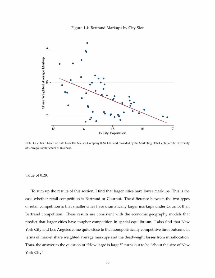
Figure 1.4: Bertrand Markups by City Size



value of 0.28.

To sum up the results of this section, I find that larger cities have lower markups. This is the

case whether retail competition is Bertrand or Cournot. The difference between the two types

of retail competition is that smaller cities have dramatically larger markups under Cournot than

Bertrand competition. These results are consistent with the economic geography models that

predict that larger cities have tougher competition in spatial equilibrium. I also find that New

York City and Los Angeles come quite close to the monopolistically competitive limit outcome in

terms of market share weighted average markups and the deadweight losses from misallocation.

Thus, the answer to the question of “How large is large?” turns out to be “about the size of New

York City”.

30

Figure 1.5: Cournot Markups by City Size



1.5.5 Gains from retail store variety

Next, I will consider the gains from retail store variety. The magnitude of differences in gains

from store variety across counties depends on differences in the number of stores across counties.

We saw earlier in the data section that there are large differences in the number of stores across

US counties. This suggests that we should expect that gains from store variety will be important.

Remember that the county price index can be written as:


σs − 1ln Nct −

1σs − 1

ln

[1

Nct∑

k∈Rct

Skt

S̃st

]− ln ϕ̃st

The first term captures the average product variety adjusted store price index. The second term

captures the gains from retail store variety. Since the estimated elasticity of substitution across

stores is estimated to be less than infinite, I expect there will be consumer gains from greater

retail variety in larger counties.

31

Figure 1.10 shows the overall county price indices (in levels), plotted by county population.

The figure shows that county price indices dramatically fall with county size. The regression

line has a slope of -0.0013 and is significantly different from zero at the 1% level. Los Angeles

County, the largest county, has a price index half that of counties with a population of 150,000

people. This is evidence for important consumption-based agglomeration forces in the US.

Figure 1.6: County Price Index by County Size



Since the county price index reflects both retail store variety and differences in tradable prod-

uct variety across counties, I will decompose it into the multiple terms to isolate the effects of

retail store variety. First, I will investigate differences in the first term of the welfare equation

which reflects differences in tradable product variety for the (geometric) average store in the

county. Then I will investigate specifically the consumer gains from store variety.

Figure 1.7 shows the log of the geometric mean store price index by log county population.

The figure shows that the average store price index is larger for larger counties. The regression

line has a slope of 0.013 and is significantly different from zero at the 5% level. This shows that

32

even accounting for product variety at the store level, the average store in the largest counties

has a higher price index than in smaller counties. Therefore, the negative relationship between

the county price index and county size is not driven by differences in tradable product variety

across counties.

Figure 1.7: Average Store Price Index by County Size



Figure 1.8 shows the gains from store variety by county size. The results show that the

county price index falls dramatically with county size because of large differences in retail store

variety. The regression line has a slope of -0.21 and is significantly different from zero at the 1%

level. These results suggest that non-tradable services, in this case retail services, are necessary

to generate large consumption-based agglomeration forces.

A concern one might have with this store variety result is that it may not be surprising that

large counties contain a lot more stores. The largest county in particular, Los Angeles County,

is very large. To consider the robustness of the variety result, Figure 1.9 shows the retail store

variety adjusted price index using truncated (first 3 digit) zip codes instead of counties. There

33

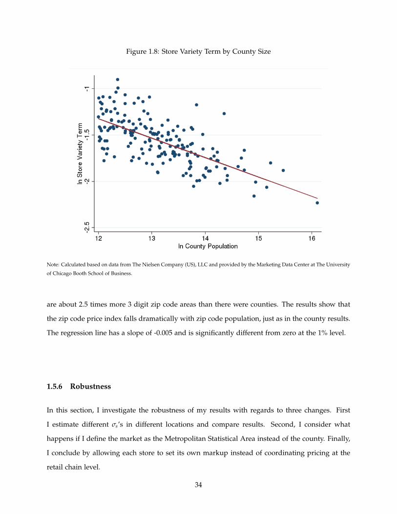
Figure 1.8: Store Variety Term by County Size



are about 2.5 times more 3 digit zip code areas than there were counties. The results show that

the zip code price index falls dramatically with zip code population, just as in the county results.

The regression line has a slope of -0.005 and is significantly different from zero at the 1% level.

1.5.6 Robustness

In this section, I investigate the robustness of my results with regards to three changes. First

I estimate different σs’s in different locations and compare results. Second, I consider what

happens if I define the market as the Metropolitan Statistical Area instead of the county. Finally,

I conclude by allowing each store to set its own markup instead of coordinating pricing at the

retail chain level.

34

Figure 1.9: Store Variety Term by County Size



1.5.6.1 Heterogeneity in σs

In the earlier results I relied on a common estimate of σs across locations. In this section, I inves-

tigate the robustness of my markup and price index results to allowing heterogeneity in σs across

locations. The misallocation results are qualitatively unchanged after relaxing the assumption of

a common σs.

Table 1.8 reports results for estimating different σs parameters for different portions of the

city size distribution. Splitting the set of cities in half and estimating a different σs for each

half produces estimates not too far on either side of the base σs estimate of 4.5. Larger cities

are estimated to have a higher elasticity of substitution across stores. The two estimates are

statistically different at the 5% level.

Table 1.8 also shows results after splitting the data into quartiles by city size. The results are

very similar to splitting the sample in half. In the point estimates, larger cities have a higher

35

Table 1.8: σs Estimates by City Size Dist.

1st Half of Cities by Size 2nd Half of Cities by SizeIV Estimate σs (95% CI) 3.9 (3.5, 4.3) 4.7 (4.5, 5.0)

City Size Dist. 1st Quartile 2nd Quartile 3rd Quartile 4th QuartileIV Estimate σs (95% CI) 3.9 (3.4, 4.5) 3.9 (3.4, 4.4) 4.5 (4.2, 4.9) 4.8 (4.5, 5.1)


elasticity of substitution across stores. However, the confidence intervals across quartiles almost

overlap for all quartiles. The benchmark σs estimate of 4.5 is contained in 3 out 4 quartile

confidence intervals, and almost contained in the remaining quartile confidence interval.

Table 1.9 shows results for estimating a different σs for every city. The median estimate is

very close to the benchmark estimate of 4.5. The confidence intervals overlap for nearly all

the percentiles shown. I cannot reject that the true σs equals 4.5 for the majority of the cities.

I conclude that the differences in the estimated σs parameters across cities are mostly due to

lack of precision from estimating on small sample sizes, since I find no correlation between the

estimated σs parameters and either city size or density (not shown).

Table 1.9: σs Estimates by MSA

Percentile σs10 3.6 (2.2, 4.2)25 3.8 (2.6, 5.1)50 4.7 (3.1, 6.0)75 5.7 (4.1, 7.9)90 7.1 (4.9, 10.1)


Having estimated different σs parameters across locations, I will next see how these differ-

ences matter for the markup results discussed earlier. I will first consider the two σs parameters

estimated by splitting the cities into two groups by size. I will then consider the set of city-level

σs estimates.

Figure 1.10 shows the relationship between the Bertrand markups and city size when using

the σs estimates from each half of the city size distribution. Since the point estimates imply that

larger cities have a higher elasticity of substitution across stores, these results only reinforce the

36

prior result that larger cities have lower markups. These two σs’s imply that even monopolis-

tically competitive retail chains (with near-zero market shares) charge lower markups in larger

cities. The monopolistically competitive markup in the smaller half of cities is about 0.35, while

the monopolistically competitive markup in the large half of cities is 0.26. With these estimates,

the share weighted average markup in Des Moines is now estimated to be about 17 percentage

points higher than in New York.

Figure 1.10: Bertrand Markups for Two σs Case



Figure 1.11 shows the relationship between the Cournot markups and city size when I es-

timate a different σs for every city. Larger cities are still estimated to have statistically and

economically significantly lower markups in the Cournot case. New York still has a markup

that is about 30 percentage points lower than Des Moines. In the Bertrand case, the slope of the

best fit line is nearly the same as in the benchmark one σs case. However, the large range of σs

estimates adds a lot of noise and the Betrand markup slope is no longer statistically significant.

Next, consider the robustness of the variation in county price indices to heterogeneity in σs.

37

Figure 1.11: Cournot Markups for MSA σs Case



Figure 1.12 plots the county price indices using the estimate of σs from each half of the city size

distribution. Despite differences in the gains from store variety across small versus large cities,

the results are nearly unchanged from the base case considered earlier. The largest county (Los

Angeles County) still has a price index that is half of counties with populations of 150,000 people.

This relationship is statistically significant at the 1% level.

Figure 1.13 plots the county price indices using the estimates of σs for each city. There is

significantly more variation in county price indices in this case relative to the base case, driven

by heterogeneity in the gains from retail store variety across cities. However, the relationship

between the price indices and county size remains robust. The regression slope is still negative

and statistically significant at the 1% level. The results still imply that counties with population

of 150,000 people have a price index twice as high as the price index for Los Angeles County.

38

Figure 1.12: County Price Indices for Two σs Case



1.5.6.2 MSA market definition

In the earlier results the relevant market is the county. I now consider the robustness of the

markup results if instead the market is defined as the metropolitan statistical area. I also con-

struct retail store variety-adjusted city price indices using the MSA as the relevant market and

compare these price indices with city size.

Figure 1.14 plots the Bertrand markups estimated using MSA retail chain market shares

versus city size. The results are very similar to the base case. Larger cities have lower retail

markups. This relationship is statistically significant at the 1% level. Des Moines is estimated

to have about 15 percentage points higher markups relative to New York. The results for the

Cournot markups share a similar pattern, with larger variation in markups across cities.

Figure 1.15 plots city-level price indices by city size. Similar to before, larger cities have

lower variety-adjusted price indices. The regression slope is the same as before: -0.001. This

39

Figure 1.13: County Price Indices for MSA σs Case



relationship is statistically significant at the 1% level. New York still has a price index which

is about a half the level of the price index in Des Moines. Surprisingly, using a larger market

definition (MSA vs county) did not result in larger differences in price indices across locations.

1.5.6.3 Store vs Chain Market Share

In this section, I investigate whether markups still fall with city size if I allow each store to set its

own markups instead of having constant markups at the chain level. Figure 1.16 plots the share

weighted average Cournot markup in this case by city size. The finding that larger cities have

lower markups is robust, although the difference aross cities is smaller. In this case, Des Moines

has about a 6 percentage point higher markup relative to New York, compared to a difference of

30 percentage points in the base case. The estimated Bertrand markups show the same pattern,

in that larger cities have lower markups. Howver, the difference in Bertrand markups across

cities is only a few percentage points in this case.

40

Figure 1.14: Bertrand Markups using MSA Markets



1.6 Conclusion

I provide a unified framework to study three aspects of the retail sector: consumption misallo-

cation from retail markups, markup variation with city size, and the consumer gains from retail

store variety. I use detailed retail store scanner data to structurally estimate the model of con-

sumer demand and oligopolistic retail competition for 55 MSAs in the US. I use counterfactual

exercises and decompositions of the consumer price index to quantify the importance of each of

the three retail mechanisms.

My estimates show that losses from retail misallocation are economically significant. Misal-

location losses are between 1% to 4.6% of aggregate packaged goods consumption, depending

on the nature of competition. The value to consumers of this lost consumption is $918 million to

$4.4 billion per year. The deadweight loss from retail misallocation is $302 million to $2.2 billion

per year. These deadweight losses represent between 0.3% and 2.3% of total yearly sales. The

41

Figure 1.15: City Price Indices



consumption losses from retail misallocation are about the same magnitude as the losses from

producer misallocation in the US.

I also find that New York City has a lower share weighted average markup by 10 to 30

percentage points relative to Des Moines, depending on the nature of competition. Cournot

competition features larger markup differences across cities than Bertrand competition. Ad-

ditionally, New York City and Los Angeles are found to be approximately at the undistorted

monopolistically competitive limit in terms of markups and the deadweight loss from misalloca-

tion. These findings are robust to different market definitions (county vs metropolitan statistical

area) and assumptions about which decision-making unit sets markups (eg. the retail chain or

the individual stores).

My estimates imply that retail store variety significantly impacts the cost of living and could

be an important consumption-based agglomeration force. Retail store variety-adjusted county

price indices are 50% lower in the largest counties (eg. Los Angeles County) relative to coun-

42

Figure 1.16: Cournot Markups using Store Market Shares



ties with populations of 150,000 people (eg. Johnson County, Texas). This result is driven by

differences in the number of available retail stores and not by differences in available product

variety within stores across counties. These results are robust to constructing price indices using

truncated 3-digit zip code areas instead of counties.

My results have important implications for policy. Any policy change that can reduce con-

centration (eg. loosening policies that prevent entry, such as the policies used by some localities

to prevent entry of big box retailers), may be welfare improving, particularly in the smallest

cities. Policies that prevent further concentration (eg. merger policy) are also important. On the

other hand, allowing entry of big box retailers, in so far as this leads incumbent retailers to exit,

may cost consumers in terms of reduced retail store variety. Policymakers should pay careful

attention to potential trade-offs of this type.

My results also raise questions for future work to address. For example, I find much larger

differences in consumer prices indices across locations in the US than prior work in the literature.

43

This suggests that consumption-based agglomeration forces may be even more important than

economists have previously realized. We know that agglomeration forces must be counteracted

by congestion costs in such a way as to prevent everyone from moving to the largest cities. I leave

it to future work to investigate whether congestion costs such as differences in housing costs (eg.

rents) across US cities are large enough to counteract the agglomeration forces suggested by this

paper, or whether we must look elsewhere for the dispersion forces that explain the observed

equilibrium population distribution across US cities.

44

Chapter 2

What is ’Firm Heterogeneity’ in Trade Models? The Role of Quality, Scope,

Markups, and Cost (with Stephen J. Redding and David E. Weinstein)

2.1 Introduction

Why are some firms larger than others? Some companies, such as the Coca Cola Corporation,

generate billions of dollars of sales and dominate the markets in which they operate. Other

companies account for only a small fraction of the sales of their larger competitors. What ex-

plains these vast differences in firm performance? Answering this question is important for

quantifying equilibrium models of firm heterogeneity developed in the recent trade and macro

literatures and for understanding the relationship between microeconomic firm performance and

macroeconomic outcomes.

Recent research on firm heterogeneity in trade and macroeconomics (e.g. Melitz [2003], Feen-

stra [2014], Manova and Zhang [2012]) points to four components of firm heterogeneity: costs,

quality, markups and product scope (i.e., the number of products produced by firms). We de-

velop a structural model of heterogeneous multiproduct firms that can be used to decompose

the firm-size distribution into the relative contributions of each component. We first use this

framework to structurally estimate elasticities of substitution across varieties between and within

multiproduct firms. We next implement our model-based decomposition for the just over 50,000

firms that supply goods with barcodes in the Nielsen HomeScan Database in a typical quarter.

This decomposition uses the structure of the model to isolate different margins in the data with-

out making assumptions about how those margins are related to one another (as in the business

cycle decomposition of Chari et al. [2007] in the macroeconomics literature). Our framework

requires only price and expenditure data and hence is widely applicable. We separate out the

contributions of price and quality using the exclusion restriction that marginal cost only affects

firm sales through price. In contrast, quality is a demand shifter that shifts sales conditional on

45

price.1

Our results point to quality differences, which we define as average consumer utility per

physical unit of output, as being the principal reason why some firms are successful in the

marketplace and others are not. Depending on the specification considered, we find that 50-70

percent of the variance in firm size can be attributed to differences in quality, about 23-30 percent

to differences in product scope, and less than 24 percent to cost differences. When we turn to

examine time-series evidence, the results become even more stark. Virtually all firm growth can

be attributed quality improvements with most of the remainder due to increases in scope. These

results suggest that most of what economists call differences in revenue productivity reflects

differences in quality rather than cost.

Our framework uses a nested constant elasticity of substitution (CES) utility system that

allows the elasticity of substitution between varieties within a firm to differ from the elasticity

of substitution between varieties supplied by different firms. Our choice of this CES demand

structure is guided by its prominence, tractability and empirical feasibility. Across international

trade, economic geography, and macroeconomics, there is little doubt that this framework is the

preferred approach to modeling product variety. Since our approach nests the standard CES-

monopolistic competition model as a special case, we can compare our results with those that

would obtain in a standard trade, macro or economic geography model. However, we generalize

this standard model to allow firms to supply multiple products (a pervasive feature of our data)

and to have market power (since the largest firms in our data are far from being measure zero).

Incorporating these features into our structural model yields a number of additional insights.

Our model makes clear a conceptual problem in the estimation of firm productivity that is likely

to bias existing estimates. Most productivity estimates rely on the concept of real output, which

is calculated by dividing nominal output by a price index. However, the formula for any eco-

nomically motivated price index, which is the same as a unit expenditure function, is dependent

on implicit assumptions about how the output of firms enters utility. Thus, one cannot move from

nominal output to real output without imposing assumptions about the structure of the demand system.2

1Our definition of quality is standard in the literature. For example Sutton [1986] defines “’vertical’ productdifferentiation...has the defining property that if two distinct products are offered at the same price, then all consumersprefer the same one (the higher-quality product)”

2This point was stressed by Aristotle in his Nicomachean Ethics (Book V, Section 5): ”Demand holds things together

46

Our results show theoretically and empirically that the CES measure of a multiproduct firm’s

price is highly sensitive to how differentiated its output is and how many products it supplies.

The sensitivity of the CES price index to demand parameters, such as the elasticity of substitution

and whether multiproduct firms exist, implies that estimates of real output are equally sensitive

to these demand parameters. We show that if demand has a nested CES structure, conventional

measures of real output will have a downward bias that rises with firm size with an elasticity

of around one third. In other words, real output variation is substantially greater than nominal

output variation. This bias also implies that true productivity differences are much larger than

conventionally measured productivity differences.

The bias is driven by two features of reality that are typically ignored in most analyses. First,

most analyses treat producers as single-product firms so they can avoid complications arising

from the challenges of measuring the real output of multiproduct firms. However, our results

indicate that multiproduct firms are the norm. For example, we document that 70 percent of

firms supply more than one barcode and these firms account for more than 99 percent of output

in their sectors.3 Therefore truly single product firms account for a negligible share of sales in

our data. Second, we show that if the output of multiproduct firms is differentiated, the common

assumption that total firm output is simply the sum of the output of each good understates real

output for multiproduct firms, and the degree of this downward bias rises in the number of

products supplied.

Our framework also provides a new metric for quantifying the extent to which a firm’s

products are differentiated from those of its rivals. If a firm’s products are perfectly substitutable

with each other but not with those of other firms, then 100 percent of a new product’s sales will

come from the firm’s existing sales, which implies a cannibalization rate of one. However, if a

firm’s market share is negligible (as it is for most firms) and its products are as differentiated

from each other as they are from products supplied by other firms, none of a new product’s sales

will come at the expense of the firm’s other products, which implies a cannibalization rate of

as a single unit.... In truth it is impossible that things differing so much should become commensurate, but withreference to demand they may become so.” (see http://classics.mit.edu/Aristotle/nicomachaen.5.v.html)

3By contrast, U.S. Census of Manufactures data indicates that producers of multiple five-digit Standard IndustrialClassification (SIC) products account for 37 percent of firms and 87 percent of shipments (Bernard et al. [2010]). Thedifference comes from defining single product firms as one-industry firms as opposed to one-barcode firms.

47

zero. We estimate that the cannibalization rate for the typical firm is about 50 percent, indicating

that although products supplied by the same firm are more substitutable with each other than

with those of other firms, it is not correct to think of them as perfect substitutes.

We find that the monopolistic competition benchmark of atomistic firms with constant markups

provides a good approximation for the vast majority of firms. The reason is simple. Most firms

have trivial market shares and hence are unable to exploit their market power. However, there

is substantial variation in markups for the very largest firms that account for disproportionate

shares of aggregate sales. This variation is greater under quantity competition than under price

competition. In most sectors, the largest firm has a market share above 20 percent, which enables

it to charge a markup that is thirty percent higher than that of the median firm under price

competition and double that of the median firm under quantity competition. We use the model

to undertake counterfactuals, in which we show that these variable markups for the largest firms

have quantitatively relevant effects on aggregate welfare and the firm sales distribution.

The remainder of the paper is structured as follows. Section 2.2 reviews the related literature.

Section 2.3 discusses the data. Section 2.4 introduces the model. Section 2.5 uses the structure of

the model to derive moment conditions to estimate elasticities of substitution and undertake our

decomposition of firm sales. Section 2.6 presents our estimation results. Section 2.7 undertakes

counterfactuals. Section 2.8 concludes.

2.2 Related Literature

Over the last decade, the fields of international trade and macroeconomics have undergone a

transformation as the dissemination of micro datasets and the development of new theories

has led to a shift in attention towards firm heterogeneity. Existing research has suggested a

number of candidate explanations for differences in firm performance, including differences in

production efficiency (e.g. Melitz [2003]), product quality (e.g. Eslava et al. [2014], Johnson [2012],

Khandelwal [2010], Schott [2004]), markups (e.g. De Loecker and Warzynski [2012], De Loecker

et al. [2014]), fixed costs (e.g. Das et al. [2007]), and the ability to supply multiple products (e.g.

Arkolakis and Muendler [2010], Bernard et al. [2010], Bernard et al. [2011], Eckel et al. [2013],

Eckel and Neary [2010], Mayer et al. [2014]). While existing research typically focuses on one or

48

more of these candidate explanations, they are all likely to operate to some degree in the data.

We develop a general theoretical model that incorporates each of these candidate explanations

and estimate that model structurally using disaggregated data on prices and sales by firm and

product. We use the estimated model to provide evidence on the quantitative importance of each

source of firm heterogeneity and the ways in which they interact with one another.

In much of the literature on firm heterogeneity following Melitz [2003] productivity and

product quality are isomorphic. Under the assumption of CES preferences and monopolistic

competition, productivity and product quality enter equilibrium firm revenue in exactly the

same way. However, these different sources of firm heterogeneity have different implications for

firm revenue conditional on prices (e.g. Berry [1994], Khandelwal [2010]). While productivity

only affects firm revenue through prices, product quality is a demand-shifter that shifts firm

revenue conditional on prices. An advantage of our approach is that we observe prices and sales

in our data, and hence we are able to separate these two sources of dispersion of firm sales.4

Most of the existing research on firm heterogeneity in trade and macroeconomics has as-

sumed that firms are atomistic and compete under conditions of monopolistic competition (e.g.

Melitz [2003] and Melitz and Ottaviano [2008]). In contrast, a small number of papers have al-

lowed firms to be large relative to the markets in which they operate (e.g. Atkeson and Burstein

[2008], Amiti et al. [forthcoming], and Edmond et al. [2012]). When firms internalize the effects

of their decisions on market aggregates, they behave systematically differently from atomistic

firms. Even under CES demand, firms charge variable mark-ups, because each firm internalizes

the effects of its pricing decisions on market price indices and these effects are greater for larger

firms.5 Furthermore, since firms are of positive measure, idiosyncratic shocks to these “granu-

lar” firms can affect aggregate outcomes, as in Gabaix [2011] and Di Giovanni and Levchenko

[forthcoming]. In contrast to these papers, we structurally estimate a model of heterogeneous

firms, and show how it can be used to recover the determinants of the dispersion of firm sales

and undertake counterfactuals.

4Our CES formulation of market demand can be derived from a discrete choice model of the demands of individ-ual consumers, as shown in Anderson et al. [1992].

5Our model generates variable mark-ups without a “choke price” above which demand is zero. Therefore thismodel lies outside the classes considered by Arkolakis et al. [2012a] and Arkolakis et al. [2012b], in which aggregatestatistics such as the trade share and trade elasticity are sufficient statistics for the welfare gains from trade.

49

To the extent that such large firms supply multiple products, they take into account the effect

of introducing new varieties on the sales of existing varieties. Most of the existing theoretical

research on multiproduct firms in trade and macroeconomics has abstracted from these canni-

balization effects by again assuming atomistic firms (e.g. Agur [2010], Allanson and Montagna

[2005], Arkolakis and Muendler [2010], Bernard et al. [2010], Bernard et al. [2011], Mayer et al.

[2014] and Nocke and Yeaple [2006]). Important exceptions that explore cannibalization effects

theoretically are Feenstra and Ma [2008] , Eckel and Neary [2010], and Dhingra [2013]. In contrast

to these theoretical studies, we develop a structural model that can be used to provide quanti-

tative evidence on how important it is to introduce such cannibalization effects into models of

firm behavior.

Most existing empirical research on multiproduct firms has measured products using pro-

duction classification codes (e.g. around 1,500 five-digit Standard Industrial Classification (SIC)

categories in Bernard et al. [2010]) or trade classification codes (e.g. around 10,000 Harmonized

System codes in Bernard et al. [2009] ). In contrast, we measure products at a much finer level

of resolution using what we term “barcodes”—either 12-digit Universal Product Codes (UPCs)

or 13-digit European Article Numbers (EANs)—in scanner data.6 This measure corresponds

closely to the level at which product choice decisions are made by firms, because it is rare for an

observable change in product attributes to occur without the introduction of a new barcode.

Our econometric approach builds on the literature estimating elasticities of substitution and

quantifying the contribution of new varieties to welfare following Feenstra [1994] and Broda and

Weinstein [2006]. We extend this estimation approach to allow firms to be of positive measure

relative to the market and to supply multiple products. We show how this extended approach

can be used to recover demand heterogeneity, marginal cost heterogeneity, variable markups,

and cannibalization effects. While a number of other studies have used scanner data, including

Broda and Weinstein [2010] and Chevalier et al. [2003], so far these data have not been used to

estimate a structural model of heterogeneous multiproduct firms and quantify the sources of

dispersion in the firm-size distribution.

6Recently, the 12-digit UPCs have been upgraded to 13-digit EAN-13s (European Article Numbers). The extradigit of the EAN-13 allows for more products and firms.

50

2.3 Data

Our data source is the Nielsen HomeScan database which enables us to observe price and sales

information for millions of products with a barcode.7 Barcode data have a number of advantages

for the purpose of our analysis. First, since barcodes are inexpensive but provide sellers access

to stores with scanners as well as internet sales, producers have a strong incentive to purchase

barcodes for all products that have more than a trivial amount of sales.8 This feature of the

data means that it is likely we observe all products supplied by firms. Second, since assigning

more than one product to a single barcode can interfere with a store’s inventory system and

pricing policy, firms have a strong incentive not to reuse barcodes. This second feature of the

data ensures that in general identical goods do not have different barcodes. Thus, a barcode is

the closest thing we have empirically to the theoretical concept of a good. Finally, since the cutoff

size for a firm is to make a sale rather than an arbitrary number of workers, we actually observe

something close to the full distribution of firms.

Nielsen collects its barcode data by providing handheld scanners to on average 55,000 house-

holds per year to scan each good purchased that has a barcode.9 Prices are either downloaded

from the store in which the good was purchased, or they are hand entered, and the household

records any deals used that may affect the price. These households represent a demograph-

ically balanced sample of households in 42 cities in the United States. Overall, the database

covers around 30 percent of all expenditure on goods in the CPI.10 We collapse the household

dimension in the data and collapse the weekly purchase frequency in order to construct a na-

tional quarterly database by barcode on the total value sold, total quantity sold, and average unit

value.11

7Our results are calculated based on data from The Nielsen Company (US), LLC and provided by the MarketingData Center at The University of Chicago Booth School of Business. Information on availability and access to the datais available at http://research.chicagobooth.edu/nielsen

8GS1 provides a company with up to 10 barcodes for a $250 initial membership fee and a $50 annual fee. There aredeep discounts in the per barcode cost for firms purchasing larger numbers of them (see http://www.gs1us.org/get-started/im-new-to-gs1-us)

9The data for 2004 through 2006 come from a sample of 40,000 households, while the data for 2007 through 2011come from a sample of 60,000 households.

10For further discussion of the Nielsen data, see Broda and Weinstein [2010].

11One question that naturally arises is whether it is appropriate to think of US firms competing in a national marketor in different regional markets. Handbury and Weinstein [forthcoming] argue there is not that much heterogeneity

51

Defining products as goods with barcodes has a number of advantages over defining goods

by industry classifications. While industry classifications aggregate products produced by a firm

within an industry, our data reveals that large firms typically sell hundreds of different products

within even a narrowly-defined sector. In other words, while prior work equates multiproduct

firms with multi-industry firms, our data hews extremely closely to what an economist would

call a multiproduct firm. In principle, it could be appropriate to aggregate all output of a firm

within an industry into a single good (Is whole milk the same as skim milk? Is a six-pack of

soda the same as a two-liter bottle?) However, as we will show theoretically, the validity of this

procedure depends on the elasticity of substitution between the products supplied by a firm,

which is an empirical question.

Instead of relying on product data for a single industry, we observe virtually the entire uni-

verse of goods purchased by households in the sectors that we examine. Our database covers

approximately 1.4 million goods purchased at some point by households in our sample. The data

were weighted by Nielsen to correct for sampling error. For example, if the response rate for a

particular demographic category is low relative to the census, Nielsen re-weights the averages so

that the price paid and the quantity purchased is representative of the United States as a whole.

Nielsen organizes the barcodes into product groups according to where they would likely

be stocked in a store. The five largest of our 100 product groups are carbonated beverages, pet

food, paper products, bread and baked goods, and tobacco. Output units are common within

a product group: typically volume, weight, area, length, or counts. Importantly, we deflate by

the number of units in the barcode, so prices are expressed in price per unit (e.g., price per

ounce). When the units are in counts, we also deflate by the number of goods in a multipack, so,

for instance, we would measure price per battery for batteries sold in multipacks. While about

two thirds of these barcoded items correspond to food items, the data also contains significant

amounts on information about non-food items like medications, housewares, detergents and

in the price levels of barcoded goods across cities. Similarly, we find that national and regional expenditure sharesand prices are strongly correlated in the data. National brands and firms (brands and firms that sell in 10 or morecities) account for 97 and 98 percent of expenditure respectively in cities with more than 1,000 households in theAC Nielsen data. Regressing city prices in these cities on national prices, quarter-year dummies, and barcode fixedeffects, we find a partial R2 (i.e., an R2 not inclusive of the fixed effects) of 0.88 and 0.73 for price levels and pricegrowth respectively. These results suggest that most of the variation in U.S. consumer prices reflects national shocksnot local ones.

52

electronics. The first few digits of the barcode identify the manufacturer.12

Table 2.1 presents descriptive statistics for our sample of firms and barcodes in the 100 prod-

uct groups. We weight the data by the sales of the product group in each year and average across

years because sectors like carbonated beverages are much larger economically than sectors like

“feminine hygiene.” There are on average 518 firms in each product group with 90 percent of the

product groups having more than 200 firms. We see enormous range in firm product scope. The

median number of products supplied by a firm is 3 and the average is 13. On average, 670,000

different UPCs were sold each quarter.

One of the most striking facts displayed in this table is the degree of firm heterogeneity. This

is manifest in the skewness of the size and barcode distributions. The largest firm in an industry

typically sells 2600 times more than the median firm. We see similar patterns in terms of product

scope and sales per product. The firm with the most products typically has 134 times more

products than the firm with the median number of barcodes, and the barcode with the most

sales on average generates almost almost a thousand times more revenue than the revenue of the

median barcode.

Table 2.1: Sample Statistics

Mean Median Std. Dev. 10thPercentile

90thPercentile Max Value

No. Firms per Product Group 518 416 309 200 942 1434Firm Sales 4141 152 25836 5 4599 402350

Log Firm Sales 12 12 3 8 15 19No. of UPCs per Firm 13 3 32 1 32 405

UPC Sales 314 40 1224 2 650 36590

Note: Weighted by product group. Firm and UPC sales in thousands. Calculations on data from The Nielsen Company (US), LLC

and provided by the Marketing Data Center at The University of Chicago Booth School of Business.

We see in Table 2.2 that almost 90 percent of sales in a product group was produced by firms

with sales in the top decile of sales. Table 2.3 provides a more detailed description of this firm

heterogeneity by focusing on the ten largest firms in each product group (where we weight the

averages by the sales of the product group). Table 2.3 reveals an almost fractal nature of firm

sales. Around two-thirds of all of the sales of firms in the top decile is produced by the ten largest

12Firm prefixes are usually seven digits but they can be as long as eleven digits, so we use GS1 data to map thebarcodes into firm identifiers. We could not obtain a firm identifier for just under 5 percent of the barcodes, and sowe dropped these products.

53

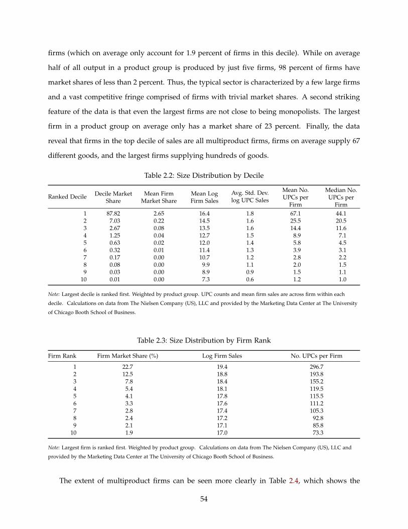
firms (which on average only account for 1.9 percent of firms in this decile). While on average

half of all output in a product group is produced by just five firms, 98 percent of firms have

market shares of less than 2 percent. Thus, the typical sector is characterized by a few large firms

and a vast competitive fringe comprised of firms with trivial market shares. A second striking

feature of the data is that even the largest firms are not close to being monopolists. The largest

firm in a product group on average only has a market share of 23 percent. Finally, the data

reveal that firms in the top decile of sales are all multiproduct firms, firms on average supply 67

different goods, and the largest firms supplying hundreds of goods.

Table 2.2: Size Distribution by Decile

Ranked Decile Decile MarketShare

Mean FirmMarket Share

Mean LogFirm Sales

Avg. Std. Dev.log UPC Sales

Mean No.UPCs per

Firm

Median No.UPCs per

Firm1 87.82 2.65 16.4 1.8 67.1 44.12 7.03 0.22 14.5 1.6 25.5 20.53 2.67 0.08 13.5 1.6 14.4 11.64 1.25 0.04 12.7 1.5 8.9 7.15 0.63 0.02 12.0 1.4 5.8 4.56 0.32 0.01 11.4 1.3 3.9 3.17 0.17 0.00 10.7 1.2 2.8 2.28 0.08 0.00 9.9 1.1 2.0 1.59 0.03 0.00 8.9 0.9 1.5 1.1

10 0.01 0.00 7.3 0.6 1.2 1.0

Note: Largest decile is ranked first. Weighted by product group. UPC counts and mean firm sales are across firm within each

decile. Calculations on data from The Nielsen Company (US), LLC and provided by the Marketing Data Center at The University


Table 2.3: Size Distribution by Firm Rank

Firm Rank Firm Market Share (%) Log Firm Sales No. UPCs per Firm

1 22.7 19.4 296.72 12.5 18.8 193.83 7.8 18.4 155.24 5.4 18.1 119.55 4.1 17.8 115.56 3.3 17.6 111.27 2.8 17.4 105.38 2.4 17.2 92.89 2.1 17.1 85.8

10 1.9 17.0 73.3

Note: Largest firm is ranked first. Weighted by product group. Calculations on data from The Nielsen Company (US), LLC and

provided by the Marketing Data Center at The University of Chicago Booth School of Business.

The extent of multiproduct firms can be seen more clearly in Table 2.4, which shows the

54

results of splitting the data by the number of UPCs supplied by a firm. While single product firms

constitute about one third of all firms on average, these firms account for less than one percent

of all output. In other words virtually all output is supplied by multiproduct firms. Moreover,

the fact that over ninety percent of output is sold by firms selling eleven or more varieties and

two-thirds of all output is supplied by firms selling more than fifty varieties, suggests that single

product firms are more the exception than the rule.

Large firms not only sell more products but they also sell a lot more of each product. The

penultimate column of Table 2.4 documents that while the typical barcode sold by a single-

product firm only only brings in $65,4000 in revenue, the typical barcode sold by a firm selling

over one hundred barcodes brings almost twice as much ($122,500). In other words, large firms

not only supply more products but they sell more of each product. If firms differed only in the

fixed cost of adding new varieties, one would not expect to see large firms sell more of each

variety. The fact that they do strongly suggests that large firms must also differ in the marginal

cost or quality of their output.

Table 2.4: Size Distribution by Number of UPCs

No. of UPCs No. of FirmsShare of Value

(%)Mean Sales

(Thousands)Median Sales(Thousands)

Avg. St. Dev.UPC Sales

1 165 0.9 73 654472–5 171 3.7 327 69802 1.31

6–10 63 4.9 1207 56096 1.5011–20 48 8.9 2924 66186 1.5721–50 44 19.1 7823 66474 1.65

51–100 18 18.7 23385 119190 1.73> 100 10 43.9 123156 122528 1.80

Note: Weighted by product group. To get last column, calculate standard deviation over log UPC sales by product group, then take

weighted average across product groups. Calculations on data from The Nielsen Company (US), LLC and provided by the

Marketing Data Center at The University of Chicago Booth School of Business.

In sum, our overview of the data reveals some key features that we model in our empirical

exercise. First, the vast majority of firms have trivial market shares, which means that if we

believe that all firms may have some market power, we need to work with demand systems that

do not imply that firms with trivial market shares have trivial markups. Second, the fact that

most economic output is produced by multiproduct firms impels us to build this feature directly

into the estimation system and allow for both differences in the fixed cost of developing new

products as well as cost and quality differences among products. Finally, the fact that there are

55

firms with non-trivial market shares implies that at least some firms are likely to have market

power. To the extent that these large firms internalize the effects of their price choices on market

aggregates, this concentration of market shares will induce departures from the monopolistic

competition benchmark.

2.4 Theoretical Framework

Our choice of functional forms is motivated not only by the data issues we identified above but

also by some theoretical concerns. Since much of the theoretical literature in international trade

and economic geography has worked with CES models, we want our results to nest this case (at

least within product groups), so that our results easily can be compared with existing work in

trade, macro and regional economics. However, we also need a framework that allows the elas-

ticity of substitution for products supplied by the same firm to be different than that for products

supplied by different firms, thereby to allow for the possibility of cannibalization effects. Finally,

we need a setup that can be applied to firm-level data without imposing implausible assump-

tions or empirical predictions. This last requirement rules out two common demand systems:

linear demand and the symmetric translog. A linear demand system would be problematic in

our setting because one needs to impose the assumption that income elasticities are equal to zero

and the estimation of marginal costs derived from a linear demand system can often result in

negative values. While the symmetric translog demand system improves on the linear demand

system in this regard, it is a difficult system to implement at the firm level because it has the

undesirable result that firms with negligible market shares have negligible markups.

Our estimation strategy therefore is based on an upper level Cobb-Douglas demand sys-

tem across product groups with CES nests below it. The upper-level Cobb-Douglas assump-

tion dramatically simplifies the estimation process because its implication of constant product

group expenditure shares allows us to assume that firms supplying different classes of prod-

ucts, e.g. carbonated beverages and pet food, do not interact strategically. However, the nested

CES structure within broadly defined “product groups” allows for strategic interactions among

firms supplying similar products. Within this structure the real consumption of each product

group is composed of the real consumption of each firm’s output, which itself is made up of the

56

consumption of each of the varieties supplied by the firm.

2.4.1 Demand

In order to implement this approach, we assume that utility, Ut, at time t is a Cobb-Douglas

aggregate of real consumption of each product group, Cgt:

Ut = ∏g∈G

Cϕgtgt , ∑

g∈Gϕgt = 1,

where g denotes each product group, ϕgt is the share of expenditure on product group g at time

t.13 Within product groups, we assume two CES nests for firms ( f ) and UPCs (u). The first nest

for firms enables us to connect with the existing literature on measuring firm productivity. The

second nest for UPCs enables us to incorporate multi-product firms. Therefore the consumption

indices for product groups and firms can be written as follows for tier of utility j ∈ {g, f }:

Cjt =

[∑

k∈Kt

(ϕktCkt)σKg−1

σKg

] σKgσKg−1

, σKg > 1, ϕkt > 0, (2.1)

where k is the tier of utility below j (i.e., if j corresponds to firm f , k corresponds to UPCs u,

and if j corresponds to a product group g, k corresponds to firms f ); Kt is the set of varieties

k; Ckt denotes consumption of variety k; ϕkt is the perceived quality of variety k; σKg is the

constant elasticity of substitution across varieties k for product group g. In other words, the real

consumption in any product group, g, is a function of the consumption of each firm’s output,

C f t, weighted by the quality consumers assign to that firm’s physical output at time t, ϕ f t, and

adjusted for the substitutability of the output of each firm, σFg.14 Similarly, we can write the sub-

utility derived from the consumption of a firm’s output, C f t, as a function of the consumption

of each UPC (i.e. barcode) supplied by that firm, Cut, multiplied by the quality assigned to the

13While we allow the Cobb-Douglas parameters ϕgt to change over time, we find that product-group expenditureshares are relatively constant over time, which suggests that a Cobb-Douglas functional form with time-invariantparameters would provide a reasonable approximation to the data.

14A small number of firms operate across multiple product groups. We assume that consumers view each of thesefirm-product-groups as a separate firm and that pricing and UPC introduction decisions are made for each firm-product-group separately. The Cobb-Douglas assumption for the upper tier of utility implies that no firm would havean incentive to price strategically across firm-product-groups, because product group expenditure shares are fixedby parameters. From now onwards, we refer to firm-product-groups as firms. These assumptions are also consistentwith product groups being quite distinct from one another (e.g. Carbonated Beverages versus Office Supplies) andthe vast majority of firms being active in only one product group.

57

physical output of that barcode, ϕut, and adjusted by the substitutability between the various

varieties supplied by the firm, σUg.15

There are a few features of this specification that are worth noting. First, if the elasticity of

substitution across varieties supplied by a firm, σUg, is finite, then the real output of a multiprod-

uct firm is not equal to the sum of the outputs of each product. For example, if the only reason

firms differ in size is that larger firms supply more varieties than smaller firms, then assuming

firm real output is the sum of the output of each variety will tend to understate the relative size

of larger firms. This size bias is a topic that we will explore in much more detail later. Second,

for much of what follows, we are focused on the sales decomposition within a given product

group (g), so for notational simplicity we can suppress the g subscript on σFg and σUg until we

need it again to pool results across sectors in Section 2.4.6. Third, we would expect (but do not

impose) that the elasticity of substitution across varieties is larger within firms than across firms,

i.e., σU ≥ σF. When the two elasticities are equal, our system will collapse to a standard CES

at the product-group level, and if the inequality is strict, we will show that our setup features

cannibalization effects. While our nested CES specification provides a parsimonious and natural

approach to modeling multi-product firms, we return to consider the robustness of our results

to alternative nesting structures in subsection 2.6.6 below.

Third, we allow firms to be large relative to product groups (and hence internalize their effects

on the consumption and price index for the product group). But we assume that the number

of product groups is sufficiently large that each firm remains small relative to the economy as a

whole (and hence takes aggregate expenditure Et and factor prices as given). Finally, since the

utility function is homogeneous of degree one in quality it is impossible to have a firm-quality,

ϕ f t, that is independent of the quality of the varieties produced by that firm, ϕut. We therefore

need to choose a normalization. It will prove convenient to normalize the geometric means of

the ϕut for each firm and the ϕ f t for each product group to equal one:

15Our definition of quality is the utility per common physical unit (e.g. utility per ounce of a firm’s output).However, variation in quality could either be interpreted as a difference in utility per physical unit or as variation inthe number of identical-quality unobservable sub-units within a physical unit. For example, it is isomorphic to saythat Firm A produces products with twice the utility per ounce as Firm B and to say that 1/2 an ounce of Firm A’sproduct generates as much utility as an ounce of Firm B’s product. In the latter case, an ounce of Firm A’s productwould contain two “1/2 ounce sub-units” each of which has identical quality to Firm B’s product. We think ourinterpretation of utility per physical unit is the most natural for our data.

58

∏u∈U f t

ϕut

1Nf t

=

∏f∈Fgt

ϕ f t

1Ngt

= 1, (2.2)

where U f t is the set of varieties supplied by firm f at time t, and N f t is the number of elements

of this set; Fgt is the set of firms in product group g at time t, and Ngt is the number of elements

of this set. Thus, firm average quality (ϕ f t) corresponds to a demand-shifter that affects all

products supplied by the firm proportionately, while product quality (ϕut) is a demand-shifter

that determines the relative sales of individual products within the firm.

We can gain some intuition for this framework by by using the product group “carbonated

beverages” as an example. Aggregate utility depends on the expenditure share (given by ϕgt)

and amount of consumption of goods in the carbonated-beverages product group, (given by

Cgt). The utility derived from the consumption of carbonated beverages depends on the quality

of Coke versus Perrier (ϕ f t), the amounts of each firm’s real output consumed (C f t), and the

degree of substitutability between Coke and Perrier (σF). Finally, the real amount of Coke or

Perrier consumed (C f t) depends on the number of different types of soda produced by each

company (U f t), the quality of each of these types of soda (ϕut), the consumption of each variety

of soda (Cut), and how similar varieties of Coke (or Perrier) products are with other varieties

offered by the same company (σU).

It turns out that it also will be useful to also work with the exact price index for consumption:

Pjt =

[∑k∈K

(Pkt

ϕkt

)1−σk] 1

1−σk

. (2.3)

Without loss of generality, we index varieties k in a given year t from the largest in terms of sales

to the smallest, and we denote the variety with the largest sales in a given year by k.

Using the properties of CES demand, the expenditure share of variety k within tier j (Skt) is

equal to the elasticity of the price index for tier j with respect to the price of variety k and is

given by the following expression:

Skt =(Pkt/ϕkt)

1−σK

∑k∈Kt (Pkt/ϕkt)1−σK

=dPjt

dPkt

Pkt

Pjt. (2.4)

Equation (2.4) makes clear exactly how we conceive of quality in this setup. Holding fixed prices,

a UPC with higher quality will have higher market shares. Similarly, holding fixed prices, firms

59

that supply higher quality goods will have greater market shares.

The role of both firm and product quality also can be seen by writing down the demand for

the output of each variety:

Cut = ϕσF−1f t ϕσU−1

ut EgtPσF−1gt PσU−σF

f t P−σUut , (2.5)

where Egt denotes total expenditure on product group g at time t. Equation (2.5) is critical in

determining how we can use this framework for understanding the different roles played by costs

and quality for understanding the sales of a firm. While quality has a direct effect on consumer

demand independent of price, cost only affects consumer demand through price. Thus, the

specification of how cost and quality affect firm pricing decisions is crucial for our identification

strategy.

2.4.2 Technology

We allow the costs of supplying products to the market to vary across UPCs, firm-product-groups

and firms. This specification encompasses both heterogeneity in productivity across firms (as in

Melitz [2003]) and heterogeneity in productivity within firms (as in Bernard et al. [2011]). All

costs are incurred in terms of a composite factor input that is chosen as our numeraire. We

assume that the variable cost function is separable across UPCs and that supplying Yut units of

output of UPC u incurs a total variable cost of Aut (Yut) = autY1+δgut , where aut is a cost shifter

and δg > 0 parameterizes the convexity of marginal costs with respect to output. Once again,

we will suppress the g subscript on δg until Section 2.4.6. In addition, each firm faces a fixed

market entry cost of H f t > 0 (e.g. the fixed costs of headquarters operations) and a fixed market

entry cost for each UPC supplied of h f t > 0 (e.g. the fixed costs of product development and

distribution).

2.4.3 Profit Maximization

In our baseline specification, we assume that firms choose prices under Bertrand competition,

though we also report results in which firms instead choose quantities under Cournot compe-

tition. Under our assumption of CES preferences, the decisions of any one firm only affect the

decisions of other firms through the product group price indices (Pgt). Each firm chooses the set

60

of UPCs u ∈{

u f t, . . . , u f t

}to supply and their prices {Pu} to maximize its profits:

maxN f t,{Put}

Π f t =u f t

∑u=u f t

[PutYut − Au (Yut)]− N f th f t − H f t, (2.6)

where we index the UPCs supplied by the firm from the largest to the smallest in sales, and the

total number of goods supplied by the firm is denoted by N f t, where u f t = u f t + N f t.

Multiproduct firms that are large relative to the market internalize the effect of their decisions

for any one variety on the sales of their other varieties. From the first-order conditions for profit

maximization, we can derive the firm markup for each UPC, as shown in Appendix B.1:

µ f t =ε f t

ε f t − 1, (2.7)

where we define the firm’s perceived elasticity of demand as

ε f t = σF − (σF − 1) S f t = σF(1− S f t

)+ S f t, (2.8)

and the firm’s pricing rule as

Put = µ f tγut, γut = (1 + δ) autYδut, (2.9)

where γut denotes marginal cost.

One of the surprising features of this setup is that markups only vary at the firm level within

product groups.16 The intuition is that the firm internalizes that it is the monopoly supplier of

its real output, which in our model equals real consumption of the firm’s bundle of goods, C f t.

Hence its profit maximization problem can be thought of in two stages. First, the firm chooses the

price index (Pf t) to maximize the profits from supplying real consumption (C f t), which implies

a markup at the firm level over the cost of supplying real output. Second, the firm chooses the

price of each UPC to minimize the cost of supplying real output (C f t), which requires setting the

relative prices of UPCs equal to their relative marginal costs. Together these two results ensure

the same markup across all UPCs supplied by the firm within a product group. However, for

firms that operate across multiple product groups, prices are chosen separately for each product

group. Therefore markups vary within firms across product groups.

The firm’s perceived elasticity of demand (2.8) is less than the consumer’s elasticity of sub-

stitution between firms, σF. The reason is that each firm is large relative to the market and hence

16This result would also hold if we substituted nested logit demand for nested CES.

61

internalizes the effect of its pricing choices on market price indices. When the firm raises the

price of a UPC (Put) and hence the firm price index (Pf t), it reduces demand for that UPC and

raises demand for the firm’s other UPCs in (2.5). Furthermore, the rise in the firm price index

also increases the product-group price index (Pgt), which raises demand for each UPC and for

the firm as a whole in (2.5). Finally, our assumption of a Cobb-Douglas functional form for the

upper tier of utility together with the assumption that each firm is small relative to the aggregate

economy ensures that total expenditure on each product group (Egt) in demand (2.5) is constant

and unaffected by firm decisions.

Although consumers have constant elasticity of substitution preferences (σF), each firm per-

ceives a variable elasticity of demand (ε f t) that is decreasing in its expenditure share (S f t), as in

Atkeson and Burstein [2008] and Edmond et al. [2012]. As a result, the firm’s equilibrium pricing

rule (2.9) involves a variable markup (µ f t) that is increasing in its expenditure share (S f t). For a

positive equilibrium price (2.9), we require that the perceived elasticity of demand (ε f t) is greater

than one (firms produce substitutes), which requires that the elasticity of substitution between

firms (σF) is sufficiently large. As a firm’s sales becomes small relative to the product group

(S f t → 0), the mark-up (2.7) collapses to the standard constant mark-up of price over marginal

cost under monopolistic competition with atomistic multiproduct firms and nested CES prefer-

ences (see for example Allanson and Montagna [2005] and Arkolakis and Muendler [2010]).

Using the above equilibrium pricing rule, overall UPC profits (Πut) are equal to UPC variable

profits (πut(

N f t)) minus fixed costs. UPC variable profits in turn can be written in terms of UPC

revenues (PutYut), the markup (µ f t), and the elasticity of costs with respect to output (ζu ):

Πut = πut(

N f t)− h f t, (2.10)

πut(

N f t)= PutYut − Au (Yut) =

(ζuµ f t − 1

ζuµ f t

)PutYut, where ζu =

dAu (Yut)

dYut

Yut

Au (Yut)= 1 + δ.

(2.11)

That is, πut(

N f t)

denotes the variable profits from UPC u when the firm supplies N f t UPCs.

2.4.4 Cannibalization Effects

The number of UPCs supplied by each firm, N f t, is determined by the requirement that the

increase in profits from introducing an additional UPC, u f t + 1, minus the reduction in profits

62

from reduced sales of existing UPCs u ∈{

u f t, . . . , u f t

}is less than the fixed cost of introducing

the new UPC, h f t. If a firm makes N f t products in equilibrium, then it must be the case that if it

were to introduce a new good, its profits would fall, i.e.,

u f t+1

∑u=u f t

πut(

N f t + 1)−(

N f t + 1)

h f t <u f t

∑u=u f t

πut(

N f t)− N f th f t

⇔ πu f t+1,t(

N f t + 1)−

u f t

∑u=u f t

{πut

(N f t)− πut

(N f t + 1

)}< h f t. (2.12)

In the case where the number of UPCs is large and can be approximated by a continuous variable,

we obtain after some manipulation (see Appendix B.2) an expression for the “cannibalization

rate”:

− ∂Yut

∂N f t

N f t

Yut=

[(σU − σF

σU − 1

)+

(σF − 1σU − 1

)S f t

]SN f t N f t > 0, f or σu ≥ σf > 1. (2.13)

where SN f t is the share of firm revenues from the new product when firm supplies N f t products,

and S f t is the share of consumer expenditure on firm f . This cannibalization rate is defined as

the partial elasticity of the sales of existing products with respect to the number of products. This

partial elasticity captures the direct effect of the introduction of a new product on the sales of

existing products, through the firm and product group price indices, holding constant the prices

and marginal costs of these existing products.

The first term on the right hand-side captures the cannibalization rate within firms: The

introduction of a UPC reduces the firm price index (Pf t), which reduces the revenue of existing

UPCs if varieties are more substitutable within firms than across firms (σU > σF). The second

term captures the cannibalization rate across firms: The introduction of the new UPC reduces

the product-group price index (Pgt), which reduces the revenue of existing UPCs if varieties are

more substitutable within product-groups than across product-groups (σF > 1).

There are two useful benchmarks for understanding the magnitude of the cannibalization

rate in equation (2.13). In both cases, it useful to think of the introduction of a “standardized”

product that has a market share equal to the average market share of the firms other goods

(SN f t N f t = 1). If firms are monopolistic competitors, S f t ≈ 0. Moreover, if we also assume

that all products supplied by a firm are as differentiated among themselves as they are with the

output of other firms, i.e., σU = σF, then the cannibalization rate will be zero because all sales

63

revenue arising from introducing a new product will come from the sales of goods supplied by

other firms. Thus, a world with monopolistic competition and equal product differentiation is

a world with no cannibalization. Clearly, the cannibalization rate will rise if firms cease being

small S f t > 0 or if goods supplied by the same firm are more substitutable with each other than

with goods supplied by different firms: σU > σF. At the other extreme, we can assume that

goods are “perfect substitutes” within firms, i.e., σU = ∞ > σf , so that varieties are differentiated

across firms but there is no difference between varieties supplied by the same firm. In this case

the cannibalization rate will be 1 because any sales of a new product will be exactly offset by a

reduction in the sales of existing products. Thus the cannibalization rate provides a measure of

where in the spectrum ranging from perfect substitutes to equal differentiation the output of a

firm lies.

2.4.5 The Sources of Firm Heterogeneity

In this section, we use the model to quantify the contribution of the different sources of firm

heterogeneity to the dispersion in sales across firms. Nominal firm sales, E f t, is the sum of sales

across UPCs supplied by the firm:

E f t ≡ ∑uεU f t

PutCut.

Using CES demand (2.5), firm sales can be re-written as:

E f t = ϕσF−1f t EgtP

σF−1gt PσU−σF

f t ∑uεU f t

(Put

ϕut)1−σU . (2.14)

Using the firm price index (2.3) to substitute for PσU−σFf and taking logarithms, we obtain:

ln E f t = (σF − 1) ln ϕ f t + ln Egt + (σF − 1) ln Pgt +

(1− σF

1− σU

)ln

∑uεU f t

(Put

ϕut

)1−σU

,

where the final term summarizes the impact of productivity, markups, UPC quality, and the

number of products on firm sales. This final term can be further decomposed into the contri-

butions of the number of UPCs supplied by a firm (N f t), the geometric mean of marginal costs

(γ̃ f t), relative quality-adjusted marginal costs across UPCs ((γut/γ̃ut) /ϕut), and the firm markup

64

(µ f t):

ln E f t ={

ln Egt + (σF − 1) ln Pgt}

(2.15)

+

{(σF − 1) ln ϕ f t +

(σF − 1σU − 1

)ln N f t

}

+

[− (σF − 1) ln γ̃ f t]+

(σF − 1σU − 1

)ln

1N f t

∑uεU f t

(γut/γ̃ f t

ϕut

)1−σU

+ (1− σF) ln µ f t,

where

γ̃ f t =

∏u∈U f t

γut

1Nf t

and recall that γut = (1 + δ) autYδut denotes marginal cost.

Equation (2.15) decomposes firm sales into seven terms that capture the various margins

through which firms can differ in sales. Clearly these margins are related to one another, since

both the number of products and the markup are endogenous to firm quality, product quality and

marginal cost. Nonetheless, the decomposition (2.15) isolates the direct effects of firm quality,

product quality and marginal cost from their indirect effects through the number of products

and the markup.

Although our decomposition is exact for any co-movement in variables, it is easiest to obtain

intuition for this equation if we consider one-at-a-time, small movements in each variable so

that we can safely ignore interactions between different variables. We therefore will explain the

intuition for this equation in terms of small movements in each variable, and note that in general

and in our empirical implementation we will allow all variables to move simultaneously.

The seven terms in equation (2.15) can be grouped into four main elements. The first element,

contained in the first set of braces, captures market size and relative pricing. Our demand system

is homogeneous of degree one in product group expenditures, so firm sales rise one to one with

aggregate expenditures. The second term captures the impact of the product group price index

that summarizes the prices of competing varieties. Holding fixed a firm’s characteristics, an

increase in the product group price level of one percent will cause the firm’s sales to rise by

(σF − 1) percent. Here, the elasticity of substitution between firm’s output and the output of

other firms, σF, plays the crucial role of explaining how much a relative price movement affects

firm sales.

65

“Total firm quality” is captured by the second two terms in braces, which capture the impacts

of the average quality of the firm’s output, “firm quality,”and the number of products the firm

offers holding fixed average quality, “product scope”. Consider two firms that supply the same

number of products, but one firm supplies higher quality varieties (measured in utility per unit),

meaning that ϕ f t > ϕ f ′t and N f t = N f ′t. Firm f will then have a higher market share; how

much depends on the elasticity of substitution between firm output, σF. For a larger value of this

elasticity, a given difference in firm average quality will translate into a larger difference in firm

market share.

Now consider two firms that supply products of identical quality but one firm supplies more

UPCs than another (N f t > N f ′t). Here, it is easiest to think about this term in a symmetric

world in which all goods and firms have identical quality (ϕut = ϕ f t = 1) and identical marginal

cost (γut = γt), so we can just focus on the role played by product scope. Although firms

have identical qualities, they do not have identical market shares because they differ in the

number of products they offer, i.e., ln N f t > ln N f ′t. For example, if consumers treated all UPCs

identically regardless of which firm supplied them, i.e., σU = σF, firm f would sell ln(

N f t/N f ′t)

percent more output than firm f ′. More generally, if the products supplied by a firm are more

substitutable with each other than with those of other firms, σU > σF, the percentage gain in

sales accruing to a firm that adds a product will be less than one reflecting the fact that a new

product will cannibalize the sales of its existing products. Indeed the degree of cannibalization

will depend on the magnitude of σU ; as this elasticity approaches infinity, the cannibalization rate

will approach one, and all sales of new products will come from the sales of the firm’s existing

products. Hence, in this limiting case of σu → ∞, adding product scope will have no impact on

sales.

The terms in the third set of braces capture the role played by marginal costs. These costs

can be divided into average marginal cost (γ̃ f t) and “cost dispersion”. Average marginal costs

(γ̃ f t) is the more conventional measure which captures the fact that high cost firms have lower

sales in equilibrium. The second term captures the fact that a firm sells more in equilibrium as

the dispersion in the cost-to-quality ratio across its products increases. The intuition is straight-

forward. The term in logs is a form of Theil index of dispersion with the numerator being the

cost of production of each variety relative to the average and the denominator being the quality

66

of the variety relative to the average (which is always normalized to one). Consider a firm that

supplies N f t varieties of identical quality at identical cost so that ϕut = γut = γ̃ f t = 1 . Now

consider a comparative static in which we multiply γut by τ > 1 and divide γkt for all k 6= u by

τN f t−1. This change has the property of keeping average marginal costs, γ̃ f t, equal to one while

increasing the dispersion in the cost of providing each element of the production bundle. Even

though average costs are unaffected by construction, firm sales will rise because the increase in

dispersion allows the firm to supply its production bundle more cheaply by shifting its output

towards the sales of cheaper varieties. This cost-dispersion term indicates that a firm sells more

if its costs relative to quality are less evenly distributed across its varieties. Here, we also see

the first instance of the insidiousness of demand for understanding multiproduct firms—in the

nested CES case, one cannot express firm-level marginal costs without reference to the demand

parameters σF and σU .

Finally, the last term captures the role played by firm markups (µ f t), which are themselves a

function of the elasticity of substitution between firms (σF) and firm market share (S f t).

2.4.6 Firm Sales Decompositions

While the decomposition given in equation (2.15) is exact for each sector, it is difficult to use

that specification to understand the general determinants of firm size because aggregate product

group expenditures are a major determinant of firm sales. Therefore we decompose firm sales

in each product group relative to the geometric mean for that product group. Notationally, the

algebra is clearer if we reintroduce the g subscript for all the relevant variables. We can write the

sales decomposition for the average firm in product group g as

ln Egt = (σFg − 1)ln ϕgt − (σFg − 1)ln γ̃gt + ln Egt + (σFg − 1) ln Pgt

+

(1− σFg

1− σUg

)ln Ngt +(1− σUg

)ln µgt + ln

1Nu f t

∑uεU f t

(γut/γ̃ f t

ϕut

)1−σUg

gt

, (2.16)

where we define X̄gt = 1Ft

∑ f∈g X f t and Ft is the number of firms in the product group. If we

subtract equation (2.16) from equation (2.15) we obtain

67

ln E f t − ln Egt = (σFg − 1){

ln ϕ f t − ln ϕgt

}+

(1− σFg

1− σUg

) [ln N f t − ln Ngt

](2.17)

−(σFg − 1){

ln γ̃ f t − ln γ̃gt

}+(1− σFg

) (ln µ f t − ln µgt

)+

(1− σFg

1− σUg

)ln

1Nu f t

∑uεU f t

(γut/γ̃ f t

ϕut

)1−σUg

− ln

1Nu f t

∑uεU f t

(γut/γ̃ f t

ϕut

)1−σUg

gt

,

which can be written more compactly as

∆g ln E f t =

{(σFg − 1)∆g ln ϕ f t +

(1− σFg

1− σUg

)∆g ln N f t

}(2.18)

+

[− (σFg − 1)

∆g ln γ̃ f t]+

(1− σFg

1− σUg

)∆g ln

1N f t

∑uεU f t

(γut/γ̃ f t

ϕut

)1−σU

+(1− σFg

)∆g ln µ f t.

The left-hand side of equation (2.18) is the sales of firm f relative to average firm sales in

the sector, and the five terms on the right-hand side tell us the importance of relative firm

average quality, scope, average marginal costs, cost dispersion, and markups in understanding

cross-sectional differences in firm size. Moreover, we can also undertake this decomposition

for a firm’s sales growth rate by taking the first difference of equation (2.18), which in our

notation simply involves replacing ∆g with ∆g,t in the equation. We now can decompose the

cross-sectional variation in firm sales using a procedure analogous to the Eaton et al. [2004]

variance decomposition commonly used in the international trade literature. In particular, we

regress each of the components of log firm sales on log firm sales as follows:

(σFg − 1)∆g ln ϕ f t = αϕ∆g ln E f t + εϕ, (2.19)

−(σFg − 1

)∆g ln γ̃ f t = αγ∆g ln E f t + εγ, (2.20)(

1− σFg

1− σUg

)∆g ln

1N f t

∑uεU f t

(γut/γ̃ f t

ϕut

)1−σU

= αD∆g ln E f t + εa, (2.21)

(1− σFg

1− σUg

)∆g ln N f t = αN∆g ln E f t + εN , (2.22)(

1− σFg)

∆g ln µ f t = αµ∆g ln E f t + εµ, (2.23)

where each firm’s log sales is differenced relative to the largest firm in its product group. By

the properties of OLS, αϕ + αγ + αD + αN + αµ = 1. The values for each of the α’s provide us

68

with a measure of how much of the variation in the distribution of firm sales can be attributed

to each factor. If we replace ∆g with ∆g,t in the above equations, we can determine how much of

the variance in sales growth rates can be attributed to each factor. Thus, estimation of these five

equations provides us with a simple way to decompose firm sales in the cross section and in the

time series.

2.4.7 Decomposing Changes in firm average quality

When decomposing firm growth, we can go one step further and understand how much of a

firm’s change in quality is due to the introduction of new products and how much is due to

demand factors for existing products. In order to see how to do this decomposition, note that

our normalization for UPC quality implies that the geometric mean of the ϕut equals one for

each firm in each period, i.e.,

ϕ f t = ϕ f t

∏u∈U f t

ϕut

1Nf t

(2.24)

We can then can take log differences of this equation over time to yield:

∆g,t ln ϕ f t ≡ ∆ ln ϕ f t − ∆ln ϕgt = ∆ ln ϕ f t +1

N f t∑

u∈U f t

ln ϕut −1

N f ,t−1∑

u∈U f ,t−1

ln ϕu,t−1 − ∆ln ϕgt,

(2.25)

where our normalization (2.2) implies that the second and third terms are both equal to zero.

To isolate the sources of changes in firm average quality, we distinguish between UPCs that

are supplied in both periods versus those that are supplied in only one of the two periods. Let

I f t = U f t ∩U f ,t−1 denote the set of UPC’s that are supplied by firm f in both periods t and t− 1.

Similarly, define U+f t to be the set of newly introduced UPCs, i.e., the set of UPCs in U f t but not

in U f ,t−1, and U−f t to be the set of disappearing UPCs, i.e., the set of UPCs in U f ,t−1 but not in

U f t.

Noting that∣∣U f t

∣∣ = ∣∣I f t∣∣+ ∣∣∣U+

f t

∣∣∣ and∣∣U f t−1

∣∣ = ∣∣I f t∣∣+ ∣∣∣U−f t

∣∣∣, we can decompose the change

in firm average quality into quality changes for a constant set of products and quality changes

from the adding and dropping of UPCs:

69

∆g,t ln ϕ f t =

∣∣I f t∣∣∣∣U f t∣∣ 1∣∣I f t

∣∣ ∑u∈I f t

ln ϕut

− ∣∣I f t∣∣∣∣U f ,t−1∣∣ 1∣∣I f t

∣∣ ∑u∈I f t

ln ϕu,t−1

+(

∆ ln ϕ f t − ∆ln ϕgt

)(2.26)

+

∣∣∣U+

f t

∣∣∣∣∣U f t∣∣ 1∣∣∣U+

f t

∣∣∣ ∑u∈U+

f t

ln ϕut

−∣∣∣U−f t

∣∣∣∣∣U f ,t−1∣∣ 1∣∣∣U−f t

∣∣∣ ∑u∈U−f t

ln ϕu,t−1

.

The first term in braces captures quality changes for a constant set of products, and includes

the change in firm average quality (∆ ln ϕ f t), as well as the difference between average product

quality for the common set of products (in square brackets) weighted by their relative importance

in the set of products in each year. This difference adjusts changes in our measure of firm quality

for changes in our normalization due to the entry and exit of new goods. We refer to the first

term in braces in equation (2.26) as the “demand effect”. It represents the change in consumers

perceived quality of the UPCs present in both periods. If the firm does not add or eliminate any

products, the summation terms will be zero since our normalization (2.2) means that average log

product quality must be zero in all periods.

However, if the set of products changes, the summation terms will not necessarily be zero.

Product turnover can influence sales either through product upgrading, which is measured in the

second term in braces in equation (2.26), as well as through changes in the number of products,

which enters separately into our decomposition of log firms sales (2.15) above. The “product

upgrading effect” (the second term in braces in (2.26) captures quality changes arising from the

adding and dropping of products. Product upgrading depends on average product quality for

the entering and exiting products (in square brackets) weighted by their relative importance in

the set of products in each year. For example, suppose a firm introduces a new high-quality

product and retires a low-quality product leaving the number of products unchanged. In this

case, the second term in braces will be positive reflecting the fact that the firm upgraded the

average quality of its product mix.

70


Our structural estimation of the model has two components. First, given data on expenditure

shares and prices{

Sut, S f t, Put}

and known values of the elasticities of substitution {σU , σF},

we show how the model can be used to determine unique values of firm average quality (ϕ f t),

product quality (ϕut), and marginal cost shocks (aut) up to our normalization of quality. These

correspond to structural residuals of the model that are functions of the observed data and pa-

rameters and ensure that the model exactly replicates the observed data. We use these structural

residuals to implement our decomposition of firm sales from Section 2.4.5 with our observed

data on expenditure shares and prices.

Second, we estimate the elasticities of substitution {σU , σF} using a generalization of Feenstra

[1994] and Broda and Weinstein [2006] to allow allow firms to be large relative to the markets in

which they operate (which introduces variable markups) and to incorporate multiproduct firms

(so that firm pricing decisions are made jointly for all varieties). This estimation uses moment

conditions in the double-differenced values of the structural residuals {ϕ f t, ϕut, aut} and also has

a recursive structure. In a first step, we estimate the elasticity of substitution across UPCs within

firms for each product group {σU}. In a second step, we use these estimates for UPCs to estimate

the elasticity of substitution across firms for each product group {σF}.

2.5.1 Structural Residuals

We begin by showing that there is a one-to-one mapping from the observed data on expenditure

shares and prices{

Sut, S f t, Put}

and the model’s parameters {σU , σF, δ} to the unobserved

structural residuals{

ϕut, ϕ f t, aut}

.

Given known values for the model’s parameters {σU , σF, δ} and the observed UPC expen-

diture shares and prices, we can use the expression for the expenditure share given in equation

(2.4) to determine UPC qualities {ϕut} up to our normalization that the geometric mean of UPC

qualities is equal to one. These solutions for UPC qualities and observed UPC prices can be sub-

stituted into the CES price index (2.3) to compute firm price indices{

Pf t}

. These solutions for

firm price indices and observed firm expenditure shares can be combined with the CES expen-

diture share (2.4) to determine firm qualities{

ϕ f t}

up to our normalization that the geometric

71

mean of firm qualities is equal to one. Furthermore observed firm expenditure shares and the

CES markup (2.7) are sufficient to recover firm markups{

µ f t}

. These solutions for markups

and observed UPC prices and expenditures can be substituted into the CES pricing rule (2.9) to

determine the marginal cost shock (aut).

Finally, our solutions for markups and observed UPC expenditures can be combined with

CES variable profits (2.11) to obtain upper upper bounds to the fixed costs of supplying UPCs

(h f t) and the fixed costs of operating a firm (H f t). The upper bound for UPC fixed costs for each

product group (h f t) is defined by the requirement that variable profits for the least profitable

UPC within a product group must be greater than this fixed cost. Similarly, the upper bound for

firm fixed costs for each product group (H f t) is defined by the requirement that variable profits

for the least profitable firm must be greater than this fixed cost.

This mapping from the observed data on expenditure shares and prices{

Sut, S f t, Put}

and

the model’s parameters {σU , σF, δ} to the unobserved structural residuals{

ϕut, ϕ f t, aut}

does

not impose assumptions about the functional forms of the distributions for the structural resid-

uals or about their correlation with one another. When we estimate the model’s parameters

{σU , σF, δ} below, we impose some identifying assumptions on the double-differenced values

of these structural results but not upon their levels. Therefore, having recovered these structural

residuals, we can examine the functional form of their distributions and their correlation with

one another.

2.5.2 UPC Moment Conditions

We now discuss our methodology for estimating the elasticities of substitution {σU , σF} and

the elasticity of marginal costs with respect to output (δ), which uses moment conditions in

double-differenced values of the structural residuals{

ϕ f t, ϕut, aut}

. This estimation again has a

recursive structure. In a first step, we estimate the elasticity of substitution across UPCs within

firms for each product group {σU} and the marginal cost elasticity (δ). In a second step, we use

these estimates for UPCs to estimate the elasticity of substitution across firms for each product

group {σF}.

In the first step, we double-difference log UPC expenditure shares (2.4) over time and relative

72

to the largest UPC within each firm to obtain the following equation for relative UPC demand:

4k,t ln Sut = (1− σU)4k,t ln put + ωut, (2.27)

where4k,t is the double-difference operator such that 4k,t ln Sut = 4 ln Sut−4 ln Skt; u is a UPC

supplied by the firm; k corresponds to the largest UPC supplied by the same firm (as measured

by the sum of expenditure across the two years); Sut and put are directly observed in our data;

ωut = (1− σU) [4 ln ϕkt −4 ln ϕut] is a stochastic error. Since we double difference the market

shares of two UPCs supplied by the same firm, we eliminate all demand shocks that are common

across a firm’s UPCs, which leaves only demand shocks that affect the sales of one a firm’s UPCs

relative to another. For example, random demand shocks and the timing of holidays, weekends,

and meteorological events might affect the success of certain products in a firm’s lineup relative

to others.

Double-differencing the UPC pricing rule (2.9) enables us to obtain an equation for relative

UPC supply. Using the cost function (Au (Yu) = autY1+δut ), and the relationship between output

and revenue (Yut = Sut/Put), the UPC pricing rule given in equation (2.9) can be re-written as:

Put = µ f tγut = µ1

1+δ

f t (1 + δ)1

1+δ a1

1+δut S

δ1+δut .

Taking logs and double-differencing, we obtain the following equation for relative UPC supply:

4k,t ln put =δ

1 + δ4k,t ln Sut + κut, (2.28)

where the markup µ f has differenced out because it is the same across UPCs within the firm;

Sut and put are again directly observed in our data; κut =1

1+δ [4 ln aut −4 ln aut] is a stochastic

error. Since the firm markup differences out and we observe prices, our estimation approach is

the same under either price or quantity competition, and hence is robust across these different

forms of competition. Once again the double differencing within a firm eliminates shocks that

are common across a firm’s products, and the fact that a barcode uniquely identifies a product

means that changes in observable product attributes will be manifest in a change of barcode but

not in a change in aut. Therefore the supply-side shocks κut correspond to factors that affect

one variety supplied by firm but not another. These might be problems in individual plants,

exchange rate movements in the countries supplying those products, etc. We assume that these

73

idiosyncratic shocks to marginal cost, κut, are orthogonal to the idiosyncratic demand shocks,

ωut.

Following Broda and Weinstein [2006], the orthogonality of idiosyncratic demand and supply

shocks defines a set of moment conditions (one for each UPC):

G(βg) = ET

[vut(βg)

]= 0, (2.29)

where βg =

σU

δ

and vut = ωutκut. For each product group, we stack all the moment

conditions to form the GMM objective function and obtain:

β̂g = arg minβg

{G∗(βg)

′WG∗(βg)}

∀g, (2.30)

where G∗(βg) is the sample analog of G(βg) stacked over all UPCs in a product group and W

is a positive definite weighting matrix. As in Broda and Weinstein [2010], we weight the data

for each UPC by the number of raw buyers for that UPC to ensure that our objective function is

more sensitive to UPCs purchased by larger numbers of consumers.

The moment condition (2.29) for each UPC involves the expectation of the product of the

double-differenced demand and supply shocks: υ = ωutκut. From relative demand (2.27) and

relative supply (2.28), this expectation depends on the variance of prices, the variance of expen-

diture shares, the covariance of prices and expenditure shares, and parameters. Our identifying

assumption that this expectation is equal to zero defines a rectangular hyperbola in (σU , δ) space

for each UPC, along which a higher value of σU has to be offset by a lower value of δ in order

for the expectation to be equal to zero (Leontief [1929]). Therefore, this rectangular hyperbola

places bounds on the demand and supply elasticities for each UPC, even in the absence of instru-

ments for demand and supply. Furthermore, if the variances for the double-differenced demand

and supply shocks are heteroskedastic across UPCs, the rectangular hyperbolas are different for

each pair of UPCs, and their intersection can be used to separately identify the demand and

supply elasticities (Feenstra [1994]). Consistent with these identifying assumptions in Broda and

Weinstein [2006], Broda and Weinstein [2010], and Feenstra [1994]), we find that the double-

differenced demand and supply shocks are in general heteroskedastic.17

17In a White test for heteroskedasticity, we are able to reject the null hypothesis of homoskedasticity at conventional

74

2.5.3 Firm Moment Conditions

We use our estimates of the UPC elasticities of substitution {σU} from the first step to solve for

UPC quality {ϕut} and compute the firm price indices{

Pf t}

using equations (2.3) and (2.4). In

our second step, we double difference log firm expenditure shares (2.4) over time and relative to

the largest firm within each product-group, f , to obtain the following equation for relative firm

market share:

∆ f ,t ln S f t = (1− σF)∆ f ,t ln Pf t + ω f t, (2.31)

where the stochastic error is ω f t ≡ − (σF − 1)∆ f ,t ln ϕ f t.

Estimating equation (2.31) using ordinary least squares would be problematic because changes

in firm price indices could be correlated with changes in firm average quality. To find a suitable

instrument for changes in firm price indices, we use the structure of the model to write changes

in firm price indices in terms of the underlying UPC characteristics of the firm. Using the CES

expenditure shares (2.4), we can write relative UPC expenditures in terms of relative UPC prices

and relative UPC qualities:

Sut

S̃ f t=

(Put/ϕut

P̃f t/ϕ̃ f t

)1−σU

, u ∈ U f , (2.32)

where here we compare each UPC to the geometric mean of UPCs within the firm, which is

denoted by a tilde so that S̃ f t = exp{

1Nu f t

∑u∈U f tln Sut

}and P̃f t = exp

{1

Nu f t∑u∈U f t

ln Put

}. Us-

ing this expression for relative expenditure shares to substitute for product quality (ϕut) in the

CES price index (2.3), we can write the firm price index solely in terms of observed relative

expenditures and the geometric mean of UPC prices:

ln Pf t = ln P̃f t +1

1− σUln

∑u∈U f t

Sut

S̃ f t

, (2.33)

where we have used our normalization that ϕ̃ f t = 1.

Equation (2.33) decomposes the firm price index into two terms. The first term is entirely con-

ventional: the geometric mean of the prices of all goods supplied by the firm. When researchers

approximate this firm price index using firm-level unit values or the prices of representative

goods supplied by firms they are essentially capturing this component of the firm price index.

significance levels for 94 percent of product groups.

75

The second term is novel and arises because the conventional price indexes are not appropriate

for multiproduct firms. The log component of the second term is a variant of the Theil index of

dispersion.18 If the shares of all products are equal, the Theil index will equal ln N f t, which is

increasing the number of products supplied by the firm, N f t. Since the Theil index is multiplied

by (1− σU)−1 ≤ 0, the firm’s price index falls as the number of goods supplied by the firm rises.

This Theil index also increases as the dispersion of the market shares across UPCs within the

firm rises.

One can obtain some intuition for this formula by comparing it to the conventional price

indexes commonly used in economics. Firm price indexes are typically constructed by making

at least one of two critical assumptions—firms only supply one product (N f t = 1), or the goods

supplied by firms are perfect substitutes (i.e., σU = ∞). Either of these assumptions is sufficient

to guarantee that the firm’s price level equals its average price level. However, both of these

assumptions are likely violated in reality. The average price of a firm’s output prices overstates

the price level for a multiproduct firms because consumers derive more utility per dollar spent

on a firm’s production if that production bundle contains more products. Thus, the (geometric)

average firm price is a theoretically rigorous way to measure the price level of firms that produce perfect

substitutes, it overstates the prices of firms that produce differentiated goods, and this bias will tend to rise

as the number of products supplied by the firm increases.

The structure of the model implies that the dispersion of the shares of UPCs in firm expen-

diture (Sut) only affects the shares of firms in product group expenditure (S f t) through the firm

price indices (Pf t). Double-differencing equation (2.33) for the log firm price index over time and

relative to the largest firm within each product-group, we obtain:

∆ f ,t ln Pf t = ∆ f ,t ln P̃f t +1

1− σU∆ f ,t ln

∑u∈U f t

Sut

S̃ f t

, (2.34)

where the model implies that the second term on the right-hand side containing the shares of

UPCs in firm expenditure is a suitable instrument for the double-differenced firm price index

in (2.31). We find that this instrument is powerful in the first-stage regression (2.34), with a

18The standard Theil index uses shares relative to simple average shares, while ours expresses shares relative tothe geometric mean.

76

first-stage F-statistic for the statistical significance of the excluded exogenous variable that is

substantially above the recommended threshold of 10 from Stock et al. [2002]

2.6 Estimation Results

We present our results in several stages. First, we present our elasticity and quality estimates

and show that they are reasonable. Second we use these estimates to examine cannibalization,

and finally we present our results on the sources of firm heterogeneity.

2.6.1 Estimated Elasticities of Substitution

Because we estimate 100 σU’s and σF’s, it would needlessly clutter the paper to present all of

them individually. Table 2.5 shows goods supplied by the same firm are imperfect substitutes.

For UPCs, the estimated elasticity of substitution ranges from 4.7 at the 5th percentile to 17.6 at

the 95th percentile with a median elasticity of 6.9. These numbers are large compared with trade

elasticities reflecting the fact that products supplied by the same firm are closer substitutes than

products supplied by different firms. The median elasticity implies that a one percent price cut

causes the sales of that UPC to rise by 6.9 percent.19

Table 2.5: Distribution of 100 GMM Estimates

Ranked Percentile σU σF σU − σF δ

1 24.4 12.8 16.8 0.625 17.6 8.5 9.4 0.42

10 14.0 7.3 6.6 0.3025 8.6 5.1 4.0 0.2050 6.9 3.9 2.6 0.1675 5.4 3.1 2.2 0.0990 5.0 2.6 1.8 0.0699 4.4 2.1 1.2 0.02

Note: Percentiles are decreasing: largest estimate is ranked first. Calculations on data from The Nielsen Company (US), LLC and

provided by the Marketing Data Center at The University of Chicago Booth School of Business.

The fact that we estimate the different products supplied by a given firm to be imperfect

substitutes for each other has profound implications for how we should understand firm pricing

19The UPC own price elasticity derived in equation (B.2) is given by

∂CutPut

PutCut

= (σF − 1) S f tSut + (σU − σF) Sut − σU .

77

and productivity. All productivity estimates are based on a concept of real output, which, in

index number theory, equals nominal output divided by the minimum expenditure necessary to

generate a unit of utility. According to equation (2.1) the quality-adjusted flow of consumption

from a firm’s output is ϕ f tC f t, so the corresponding expenditure function for a unit of quality-

adjusted consumption is Pf t/ϕ f t. However, for multiproduct firms, the formula for Pf t depends

on the demand system, and therefore the formula for a firm’s real output also depends on the

demand system. In other words, for multiproduct firms, the concept of real output is not independent

of the demand system, so all attempts to measure productivity based on a real output concept contain an

implicit assumption about the structure of the demand system.20

This problem is more pernicious than simply saying that firm prices are measured with error;

the errors are likely to be systematic. Equation (2.33) indicates that, in the CES system, the use of

average goods prices to measure firm-level prices will overstate the price level (and understate

real output) more for large multiproduct firms than for small single-product ones. Therefore,

if the true model is CES but a researcher uses a quantity-weighted average of the prices of the

goods supplied by the firm to measure firm prices—what we term a “conventional” price index

or PConvf t —the results are likely to underestimate productivity differences.

But how big is this problem in practice? If we denote the consumer’s expenditure on a firm’s

output by E f t, we can write the conventional measure of real output, QConvf t , as E f t/PConv

f t , and

the CES measure of real output, QCESf t , as E f t/

(Pf t/ϕ f t

). These measures will vary across sectors

due to the units, so in order to compare size variation across sectors we will work with unitless

shares of each firm in total output (i.e., QCESf t / ∑ f∈g QCES

f t and QConvf t / ∑ f∈g QConv

f t ). Figure 2.1

plots these two measures of real output. As one can see in Figure 2.1, the choice of price index

matters enormously for the computation of real output. Moreover, our estimate of σU suggests

that there are large downward biases in the measurement of real output of large firms. While,

on average, the conventional measure of real output is quite close to the CES measure for small

firms it systematically understates the value of real output for firms with large market shares. We

can econometrically measure the magnitude of this bias by regressing ln(

PConvf t /

(Pf t/ϕ f t

))on

ln E f t (with product group fixed effects) and examining the coefficient on log sales. If there were

20Since firms supply differentiated products, the relevant measure of productivity is TFPR (Foster et al. [2008]),which necessarily depends on prices and hence the specification of demand.

78

no bias, we would expect a coefficient of zero, but we actually obtain a coefficient of 0.3447 (s.e.

0.0004, R2 = 0.3) indicating that failing to take into account the multiproduct nature of firms

causes us to significantly underestimate the size of large firms. This estimate is economically

significant as well. It implies that holding fixed a firm’s conventional price index, every one

percent increase in firm sales is associated with a 1.3 percent increase in its real output in a CES

model. The difference between the two estimates reflects the importance of assumptions about

demand when constructing a firm price index.

Figure 2.1: Bias in Conventional Real Output Share


A second striking feature of our estimated results is that the elasticity of substitution among

varieties supplied by a firm is always larger than that that between firms (i.e., σU > σF). It is

important to remember that this is not a result that we imposed on the data. Moreover, most of

the elasticities are precisely estimated—in 82 percent of the cases, we can statistically reject the

hypothesis that σU = σF at the 5% level. The higher elasticities of substitution across UPCs than

across firms imply that varieties are more substitutable within firms than across firms, which

implies cannibalization effects from the introduction of new varieties by firms. Moreover, the

79

fact that the estimated elasticities of substitution are always greater than one implies that firms’

varieties are substitutes, which is required for positive markups of price over marginal costs (c.f.,

equation (2.9)).

In order to assess whether our elasticities are plausible, it is useful to compare our estimates

with those of other papers. In order to do this, we restricted ourselves to comparing our results

with studies that used US scanner data and estimated elasticities for the same product groups

as ours. We do this because, as Broda and Weinstein [2006] show, elasticity estimates for ag-

gregate data can look quite different than those for disaggregate data. Unfortunately, we did

not find studies estimating the elasticity of substitution within firms, but we did find studies

that examined elasticities akin to our cross-firm elasticity, σF. Figure 2.2 plots our estimates of

σF against other estimates from Gordon et al. [2013] and the literature review contained in the

web appendix to their paper. Although these other studies use different methods, we find that

our estimates are very similar with a statistically significant correlation of 0.59 and the points

arrayed fairly close to the 45-degree line. Therefore, while our empirical approach has a number

of novel features in modeling multiproduct firms that are of positive measure relative to the mar-

kets in which they operate, the empirical estimates generated by our procedure are reasonable

compared to the benchmark of findings from other empirical studies.

2.6.2 Quality

The quality parameters are a second key component of our decomposition. Our estimation

procedure allows us to estimate a different ϕut for every quarter in our dataset. We have strong

priors that the quality of each UPC should be fairly stable across time. One way to gauge this

stability is to regress these quality parameters on UPC fixed effects in order to determine how

much of a UPC’s quality is common across time periods. When we do this and include time

fixed effects to control for inflation and other common demand shocks, we find that the R2 is

0.84, which implies that very little of the variation in our quality measures arise from changes in

UPC quality. We should also expect firm average quality, ϕ f t, to exhibit a strong firm component

but to be less stable over time. This is exactly what the data reveals. Running the same regression

for firm average quality, we find that 83 percent of the variance can be explained by firm fixed

effects. Consistent with these results, we also estimate that firm average quality exhibits more

80

Figure 2.2: Price Elasticities Compared to Literature


variation overall (not just across time) than UPC quality or marginal cost. This can be seen

in Figure 2.3, which plots kernel density estimates of UPC quality, firm average quality, and

marginal cost.

2.6.3 Markups

Using our estimated elasticities of substitution, we can compute implied firm markups. As dis-

cussed above, multiproduct firms internalize the fact that they supply a firm consumption index

and hence choose a price for each UPC that depends on the perceived elasticity of demand for

the firm consumption index as a whole (ε f t). Although demand exhibits a constant elasticity

of substitution, this perceived elasticity of demand differs across firms because they internalize

the effect of their pricing decisions on market price indices. For any firm with a strictly posi-

tive expenditure share, the perceived elasticity of demand (ε f t) is strictly less than consumers’

elasticity of substitution across varieties (ε f t < σF). Larger firms that account for greater shares

of expenditure have lower perceived elasticities of demand and hence charge higher markups of

81

Figure 2.3: Kernel Densities of Quality and Cost Estimates

UPC Quality (ϕut )

Firm Quality (ϕ f t)

Marginal Cost (γut = (1 + δ) autYδut)

Note: The UPC quality is measured by ln ϕut . Firm quality is measured byln ϕ f t, and marginal cost is computed as ln(γut/γ̃ f t

).

Calculated based on data from The Nielsen Company (US), LLC and provided by the Marketing Data Center at The University of

Chicago Booth School of Business. 82

price over marginal costs (µ f t), as summarized in equations (2.7) and (2.8) that are reproduced

below:

µ f t =ε f t

ε f t − 1,

ε f t = σF − (σF − 1) S f t.

There are two important dimensions across which markups vary. The first is cross-sector

variation with captures the fact that σF varies systematically across product groups, and the

second is within-sector variation which captures the fact that larger firms have higher markups

within a sector than smaller firms. As discussed above, our procedure for estimating the elas-

ticities {σU , σF} is robust to the assumption of either price or quantity competition, because the

firm markup differences out in (2.27) and we observe prices. However, the markup formula, and

hence the decomposition of prices into markups and marginal cost, depends in an important

way on the form of competition. In our baseline specification, we assume Bertrand competition

in prices, but we report the derivation of the markup under Cournot competition in quantities

in the appendix. A key takeaway from this comparison is that Cournot competition generates

substantially higher markups for larger firms than Bertrand competition if goods are substitutes.

Additionally, as shown in the appendix, under Bertrand competition, the relative markups of

firms depend solely on the distribution of market shares (and hence are robust to different es-

timates of the elasticity of substitution between firms). In contrast, under Cournot competition,

the relative markups of firms depend on both the distribution of market shares and the elasticity

of substitution between firms.

Table 2.6 presents data on the distribution of markups across all firms in our 100 product

groups. The median markup is 33 percent, which is slightly lower than Domowitz et al. [1988]

estimate of 36 percent for U.S. consumer goods, and slightly above the median markups es-

timated by De Loecker and Warzynski [2012] for Slovenian data which range from 17 to 28

percent. This suggests that our markup estimates are reasonable in the sense that they do not

differ greatly from those found in prior work.

While the markups of most firms are essentially the same regardless of whether we assume

firms compete through prices or quantities, the markups of the largest firms are substantially

83

Table 2.6: Distribution of Markups

Ranked Percentile Cournot Using εF Bertrand Using εF Using σF Using σU

10 0.57 0.57 0.57 0.2425 0.45 0.45 0.45 0.2350 0.33 0.33 0.33 0.1775 0.24 0.24 0.24 0.1490 0.18 0.17 0.16 0.09

Note: Markup=(Price-Marginal Cost)/Marginal Cost. Calculations on data from The Nielsen Company (US), LLC and provided by

the Marketing Data Center at The University of Chicago Booth School of Business.

different. Table 2.7 shows the distribution of the markups for the largest and second largest

firms by product group. In each case, we report the markup relative to the average markup in

the product group, so that one can see how different the markup of the largest firm is. The

median largest firm within product groups has a markup that is 24 percent larger than average

if we assume competition is Bertrand and almost double the average if we assume competition

is Cournot. However, as one can also see from this table, these markups drop off quite rapidly

for the second largest firm. Therefore, both modes of competition suggest that very few firms

can exploit their market power.

Table 2.7: Distribution of Markups Relative to Product Group Average

Cournot Bertrand

Ranked Percentile Largest Firm Second Largest Largest Firm Second Largest

10 4.68 2.59 1.73 1.2825 2.98 1.72 1.41 1.1850 1.94 1.49 1.24 1.1375 1.54 1.32 1.16 1.0990 1.37 1.23 1.10 1.06

Note: Percentiles are decreasing: largest is ranked first. Markup=(Price-Marginal Cost)/Marginal Cost. Calculations on data from

The Nielsen Company (US), LLC and provided by the Marketing Data Center at The University of Chicago Booth School of

Business.

2.6.4 Cannibalization Rate

Our estimated elasticities of substitution also determine the magnitude of cannibalization effects

in the model. As discussed above, when a multiproduct firm chooses whether to introduce a new

variety, it takes into account the impact of this product introduction on the sales of its existing

varieties. The partial elasticity of the revenue of existing UPCs with respect to the introduction

of a UPC is given by (2.13), which is reproduced below:

84

Cannibalization rate ≡[(

σU − σF

σU − 1

)+

(σF − 1σU − 1

)S f t

]SN f t N f t.

Since this cannibalization rate is defined as the partial elasticity of the sales of existing products

with respect to the number of products, and can be expressed in terms of observed expenditure

shares, it takes the same value under both price and quantity competition, as shown in the

appendix.

As we mentioned earlier, a cannibalization level of 0 corresponds to equal differentiation of a

firm’s products from its rivals and a level of 1 corresponds to a world in which the products of

firms are perfect substitutes. In Table 2.8, we present the average estimated markups and canni-

balization levels for firms by decile of size. As one can see from the table, these are remarkably

stable, which reflects the fact that even in the upper decile of firms most firms have trivial market

shares (S f ≈ 0). Interestingly, we see that cannibalization levels lie almost exactly between the

benchmarks of perfect substitutes and equal differentiation. This cannibalization level implies

that about half of the sales of a new product introduced by a firm comes from the sales of exist-

ing products and half from the sales of other firms. The fact that these cannibalization rates are

much less than one, however, underscores the fact that it is not appropriate to treat the goods

supplied by a multiproduct firm as perfect substitutes nor is it appropriate to treat multiproduct

firms as if the introduction of a new good had no impact on the sales of existing goods.

Table 2.8: Markups and Cannibalization by Decile

Ranked Decile Average Cournot Markup Average Bertrand Markup Average CannibalizationRate

1 0.40 0.38 0.512 0.38 0.37 0.503 0.37 0.37 0.504 0.37 0.37 0.505 0.37 0.37 0.506 0.37 0.37 0.507 0.37 0.37 0.508 0.37 0.37 0.509 0.37 0.37 0.50

10 0.37 0.37 0.50

Note: Largest decile is ranked first. Weighted average across product groups. Calculations on data from The Nielsen Company

(US), LLC and provided by the Marketing Data Center at The University of Chicago Booth School of Business.

Moreover, there is a slight tendency for the markups and cannibalization levels to rise with

firm size reflecting the fact that large firms have higher markups and take into account the fact

85

that more of their sales of new products comes at the expense of their existing products. We

can see this more clearly in Table 2.9, where we focus on the ten largest firms in the sector.

We estimate that the markup of the largest firm is on average 32 and 120 percent larger than

the markups of firms in the first nine deciles under price and quantity competition respectively

(comparing Tables 2.9 and 2.8), but the markup of the fifth-largest firm is not very different.

Thus, the ability to exploit market power is a feature of very few firms on average. Similarly,

cannibalization levels tend to rise for the the very largest firms. We estimate that when the largest

firm in a sector, which has an average market share of 23 percent, introduces a new product, 62

percent of the sales of that product comes from from the sales of its existing products. Since we

saw from Table 2.3 that the largest firms typically have the most products per firm, this implies

that cannibalization is likely to be a first-order issue for them.

Table 2.9: Markups and Cannibalization by Firm Rank

Firm Rank Cournot Markup Bertrand Markup Cannibalization Rate

1 0.826 0.496 0.6172 0.576 0.428 0.5653 0.498 0.407 0.5444 0.455 0.397 0.5315 0.437 0.392 0.5256 0.424 0.388 0.5217 0.415 0.385 0.5188 0.413 0.384 0.5179 0.410 0.383 0.516

10 0.403 0.382 0.514

Note: Largest firm is ranked first. Weighted averages across product groups. Calculations on data from The Nielsen Company

(US), LLC and provided by the Marketing Data Center at The University of Chicago Booth School of Business.

2.6.5 Decomposing Firm Sales

The first panel of Table 2.10 presents the decompositions described in equations (2.19) to (2.23)

for the full sample of firms and the second presents the results for the largest firms (those with

a market share in excess of 0.5 percent). We run the results over both sets of firms to see if

there are any differences between them. Overall, the results suggest a powerful role for quality

in accounting for the size of firms. The variance decomposition indicates that 76 percent of the

overall size distribution can be attributed to average quality and 21 percent is attributed to scope.

Thus, total firm quality accounts for 97 percent of variation in firm sales. If we restrict ourselves

86

to looking at the data for the fifty largest firms we still find that firm average quality explains

on average 54 percent of the variation with scope accounting for 26 percent. In other words,

even if we restrict our sample to the largest firms, quality variation accounts for 80 percent of the

variation across firms.

What is perhaps most surprising is the small role played by cost in the determination of

firm size. There are two important features of this decomposition to bear in mind. First, a

positive coefficient means that larger firms have lower costs: i.e., cost differentials help explain

size differentials. Second, our decomposition allows us to split firm-cost differentials into two

components: average marginal cost differentials and the dispersion of costs across products

(“cost dispersion”). In all cross-sectional decompositions, the cost dispersion term is positively

correlated with firm size. The intuition is simple. Larger firms tend to sell more products and

therefore are better positioned to benefit from cost differentials in supplying their consumption

index. The results for average marginal costs are more mixed. In the full sample, we find almost

no association between firm size and average costs indicating that larger firms have essentially

the same average marginal costs as smaller firms. Their total costs are lower because they can

take advantage of the cost dispersion in their output. Interestingly, we find a much stronger

association with average costs when we restrict our sample to only the largest fifty firms. Here,

we find that 18 percent of the firm size distribution can be attributed to lower average costs of

large firms and a quarter of of the overall distribution due to these cost differences. Moreover, the

results lend support to the managerial competence approach to thinking about cost differences—

large firms tend to have higher quality and lower costs. Finally markup variation, which depends

on both quality and cost through expenditure shares, plays a very small role in understanding

the firm size distribution.21

Figure 2.4 presents the results of the cross-sectional decomposition for the largest 50 firms in

each product group. Each point represents the average contribution of a particular factor towards

understanding the relative level of sales in a sector. For example, the column of points at the right

of the figure indicate that the largest firm in a product group is on average almost nine log units

larger than the average firm. Of this nine-log-unit difference the diamond-shaped point indicates

21Consistent with these findings, Roberts et al. [2011] find substantial heterogeneity in demand across Chinesefootwear producers, while Foster et al. [2013] emphasize the role of demand in the growth of entering firms.

87

Table 2.10: Variance Decompositions

Panel A: All Firms

Decomposition Quality Scope AverageMC

CostDispersion Markup Upgrading

Cross-Sectional Coefficient 0.758 0.2090 −0.036 0.0707 −0.00195Std.Error 0.002 0.0002 0.002 0.0001 0.00001

Firm Growth Coefficient 0.905 0.1571 −0.131 0.0687 −0.00059 0.0003Std.Error 0.009 0.0012 0.008 0.0010 0.00004 0.0014

Panel B: Top 50 Firms

Decomposition Quality Scope AverageMC

CostDispersion Markup Upgrading

Cross-Sectional Coefficient 0.544 0.2637 0.175 0.0613 −0.04436Std.Error 0.013 0.0016 0.013 0.0008 0.00016

Firm Growth Coefficient 0.902 0.2597 −0.163 0.0278 −0.02619 0.0233Std.Error 0.053 0.0079 0.051 0.0082 0.00131 0.0138

Note: MC is marginal cost Calculations on data from The Nielsen Company (US), LLC and provided by the Marketing Data Center

at The University of Chicago Booth School of Business.

that on average about 4.9 log units (54 percent) can be attributed to average quality differences.

The circular point reveals that about 2.3 log units (25 percent) is on average attributable to scope

differences, while the triangular and square points indicate that lower average costs and greater

cost dispersion account for about 1.3 (14 percent) and 0.6 log units (7 percent) of the sales. These

percentages are extremely similar to the percentages for larger firms that we saw in Table 2.10.

However, the fact that each set of points is relatively tightly arrayed along a line indicates that

the results presented in Table 2.10 are not the result of any outlier but are a robust feature of the

data.

There are two other features of the data that this plot also makes clear. First, we can also

see that while there is a tendency for average marginal costs to fall with size for the four largest

firms, which accounts for the upward trend in the sequence of triangular points, this upward

trend is not a robust feature of the data. This pattern helps explain why we found in Table 2.10

that average marginal costs did not fall with firm size when we looked at the full sample of firms,

but did fall when we restricted our attention to the very largest firms. Moreover, we can see that

the gains from increasing cost dispersion are a very robust feature of the data.

A second feature of the data that suggests welfare implications of the ability of the largest

firms to exploit market power is also clearly seen in Figure 2.4. We saw in Table 2.10 that

while markup variation played almost no role in understanding the firm-size distribution when

88

Figure 2.4: Sales Decomposition by Firm Rank

Note: The graph contains the weighted average across product groups of the decomposition of firm salesinto firm average quality, marginal cost, markup and product scope for the fifty firms with the largestaverage market share in 2004 and 2011. The vertical axis measures the contribution of each factor givenby the left-hand sides of equations (2.19) to (2.23). The horizontal axis is the log difference between thefirm’s sales and that of the average firm defined by the right-hand side of these equations. Calculatedbased on data from The Nielsen Company (US), LLC and provided by the Marketing Data Center at TheUniversity of Chicago Booth School of Business.

we focused on the full sample of firms, it was negatively associated with firm sales when we

examined the largest firms. Figure 2.4 shows that this negative association comes from the fact

that if it were not for the fact that the very largest two or three firms had higher markups (a

result we also saw in Table 2.9), their output levels would be higher. The implied inefficiently

low levels of output of the largest firms suggests that the monopolistic competition model breaks

down for these firms and motivates our attempt to quantify the welfare impact of this pattern in

the data in Section 2.7.

As we showed in Section 2.4.6, we can also examine the time-series determinants of firm

growth by differencing with respect to time (i.e., using ∆g,t instead of ∆g in the decompositions).

As we can see in Table 2.10, the importance of quality rises when understanding firm growth.

Virtually all of a firm’s growth can be understood in terms of increases in quality and scope

89

with cost changes playing almost no role. Interestingly, quality upgrading—i.e., the addition of

new higher quality products—plays almost no role in the typical firm’s expansion. Most of the

expansion comes from shifts in demand towards the firm’s existing products, which may reflect

marketing and other taste shifts.

Figure 2.5 presents the results from this decomposition for the fifty firms whose average

market shares in 2004 and 2011 were the highest. Thus, the column of points on the right of the

figure indicates that on average the fastest growing firm in a product group on average had sales

growth that was 1.6 log units faster than the average firm (or about 26 percent per year). Of this

faster growth, the diamond-shaped point indicates that close to one log unit (about 50 percent)

was due to quality improvements, with most of the remainder due to scope changes. The points

in these scatters are a bit less tightly distributed, indicating that there is more volatility in the

estimated determinants of firm growth than in firm shares, but the results consistently show

that the two main determinants of firm growth are firm average quality and product scope.

These results are also quite similar to to those we saw in Table 2.10, with now the new piece of

information being that we can see that the earlier results are not being driven by any particular

firm or set of firms.

Taken together, the decomposition results are quite striking in their consistency about the

sources of firm heterogeneity. Regardless of whether we examine firms in the cross-section or

in the time-series, improvements in firm average quality followed by firm scope are the most

important drivers of firm sales for both small and large firms alike. The role played by average

cost differences tends to be small and depend on the sample and decomposition method used.

But we consistently find a positive contribution towards differences in firm size from the cost

dispersion term. Finally, we see that although markup differences are unimportant determinants

of firm sales for most firms, they do appear to be important for the very largest firms something

that suggests aggregate welfare implications from the exploitation of market power by these

firms.

2.6.6 Robustness

One limitation of our approach is that to structurally estimate the model we need to assume a

particular nesting structure for demand consisting of firms and products within firms. We choose

90

Figure 2.5: Growth Decomposition the Fifty Largest Firms

Note: The graph contains the weighted average across product groups of the growth decomposition ofthe growth rate in firm sales into estimated firm average quality, marginal cost, and product scope forthe top fifty firms by average market share in 2004 and 2011. The vertical axis measures the contributionof each factor given by the left-hand sides of equations (2.19) to (2.23). The horizontal axis is the logdifference between the firm’s sales and that of the average firm growth rate defined by the right-hand sideof these equations. Calculated based on data from The Nielsen Company (US), LLC and provided by theMarketing Data Center at The University of Chicago Booth School of Business.

this nesting structure to connect with the existing literature on measuring firm productivity

(which implicitly or explicitly treats firms as a nest) and as a natural approach to modeling

multi-product firms. But it is reasonable to wonder whether our results are robust to other

nesting structures. In this section, we undertake a robustness test, in which we demonstrate that

our main finding of the importance of quality in explaining sales variation is not sensitive to our

assumed nesting structure. To do so, we use the CES functional form to derive a reduced-form

equation that can be estimated for alternative nesting structures. Although this reduced-form

equation cannot be used to recover structural parameters, it can be used to provide a lower

bound on the importance of quality variation for alternative nesting structures.

To provide evidence on the role of quality variation under alternative nesting structures,

we combine the following two results for CES demand. First, from (2.31), double-differenced

91

expenditure shares depend on double-differenced price indices for any tier of utility j. Second,

from (2.33), the price index for one tier of utility j can be expressed in terms of expenditure

shares and the geometric mean of prices for the lower tier of utility k. Combining these results,

and reintroducing the product group subscript, we obtain the following reduced-form equation

that can be estimated using OLS:

4j,t ln Sjgt = αjg + β1jg4j,t ln P̃jt + β2jg4j,t ln

[∑u∈b

Skgt

S̃jgt

]+ εjgt, (2.35)

where 4j,t is again the double-difference operator; P̃jt = exp{

1Njt

∑Njtk=1 ln Pkt

}and the error term

εjgt captures double-differenced quality.

In our structural model, the coefficient β2jg can be related to structural parameters of the

model (β2jg = 1/(σkg − 1

)). In the reduced-form regression (2.35), this coefficient does not have

a structural interpretation, because quality for tier j (εjgt) can be correlated with the geometric

mean of prices in the lower tier k (P̃jgt). Therefore, if the reduced-form regression (2.35) is

estimated using OLS, the coefficient β2jg is subject to omitted variable bias and is not consistently

estimated. For this reason, we use our structural approach developed above to estimate the

elasticities of substitution and elasticity of marginal cost {σUg, σFg, δg} for our assumed nesting

structure.

Nonetheless, the reduced-form specification (2.35) can be used to provide a lower bound on

the importance of quality for alternative nesting structures. The reason that this specification

provides a lower bound is that quality is captured in the estimated residual (ε̂jgt). Therefore,

the component of quality that is correlated with the explanatory variables is attributed to the

coefficients {β1jg, β2jg} on these explanatory variables, leaving only the orthogonal component of

quality in the estimated residual (ε̂jgt).

In Table 2.11, we report the average R2 across all product groups (g) from estimating this

reduced-form regression for alternative nesting structures, where one minus this R2 corresponds

to the variance in double-differenced expenditure shares that is unexplained by the explanatory

variables (and is instead explained by quality). We estimate the regression separately for each

product group and year, and summarize the mean and standard deviation of the R2, weighting

each product group and year by their sales.

92

In the first row of the table, we report results for our assumed nesting structure. In the re-

maining rows of the table, we report results for a wide range of alternative nesting structures.

Some of these alternative nesting structures disaggregate firms relative to our baseline specifica-

tion (e.g. Specification II uses Product Group and Brand-Module instead of Product Group and

Firm, where Brand Module distinguishes between different brands supplied by a firm, such as

Coke and Sprite soda for the Coca-Cola corporation). Other alternative nesting structures omit

firms as a nest altogether (e.g. Specification IV uses Module and Brand Module, where Mod-

ule corresponds to different types of products within a product group, such as diet and regular

soda). Across this wide range of specifications, we find that quality accounts for at least 43

percent of the variation in double-differenced sales. Thus, regardless of one’s choice of nesting

structure, it is hard to escape the conclusion that around half of sales variation is attributable to

quality variation. Since this lower bound also leaves out the important role played by scope on

demand, this further reinforces the importance of overall quality (including scope) in explaining

sales variation.

Table 2.11: Within Nest R2

Specification Nest 1 Nest 2 Nest 3 Nest 4 Mean Std. Dev.

I Product Group Firm UPC N/A 0.53 0.05II Product Group Brand-Module UPC N/A 0.46 0.07

III Product Group Firm-Module UPC N/A 0.47 0.07V Module Firm-Module UPC N/A 0.48 0.06V Module Firm-Module UPC N/A 0.49 0.05

VI Module Firm-Module Brand UPC 0.57 0.07

Note: Calculations on data from The Nielsen Company (US), LLC and provided by the Marketing Data Center at The University


2.7 Counterfactuals

We found in Table 2.9 that the monopolistic competition benchmark breaks down substantially

for the largest firms. Moreover, we learned from Figure 2.4 that the estimated exploitation of

market power by the largest firms implies reductions in these firms’ sales. We now use the

structure of the model to undertake counterfactuals to assess the quantitative relevance of our

estimated departures from monopolistic competition for aggregate welfare. We consider two

types of counterfactuals. First, we consider the implications for consumers from a regulator

93

preventing large firms from exercising their market power and thereby requiring each firm to

compete under monopolistic competition. Second, we consider the implications of allowing

firms to supply a number of differentiated products. Thus, the second type of counterfactuals

examines the gains to consumers from the different varieties supplied by each firm.

In each of these counterfactual exercises, we examine the impact on consumers under both

Bertrand and Cournot competition. In all cases, we hold constant aggregate expenditure (Et),

the sets of active UPCs and firms{

U f t, Fgt}

, and the sets of firm qualities, UPC qualities and

cost shifters{

ϕ f t, ϕut, aut}

. Therefore we abstract from general equilibrium effects through

aggregate expenditure, factor prices, and entry and exit. Our goal is not to capture the full

general equilibrium effects of each counterfactual, but rather to show that our firm-level estimates

are of quantitative relevance for aggregate outcomes such as welfare.

In the first set of counterfactuals (Counterfactuals I-B and I-C), we compare the actual equi-

librium in which firms exploit their market power with a counterfactual equilibrium in which a

price regulator requires all firms to charge the same constant markup over marginal cost equal

to the monopolistically competitive firm markup:

µ f t =σF

σF − 1. (2.36)

Moving from the actual to the counterfactual markup reduces the relative prices of successful

firms with high market shares and hence redistributes market shares towards these firms. There-

fore, we expect these counterfactuals to increase welfare and the dispersion of firm sales, but the

magnitude of these effects depends on the estimated parameters {σU , σF, δ} and the sets of firm

qualities, product qualities and cost shocks{

ϕ f t, ϕut, aut}

.

Given the assumed constant markup in equation (2.36), we solve for the counterfactual equi-

librium using an iterative procedure to solve for a fixed point in a system of five equations for

expenditure shares and price indices{

Sut, Put, S f t, Pf t, Pgt}

. These five equations are the UPC

expenditure share (given by equation (2.4) for k = u), the UPC pricing rule (equation (2.9)), the

firm expenditure share (given by equation (2.4) for k = f ), the firm price index (given by (2.3) for

k = f ) and the product group price index (given by equation (2.3) for k = g). We use the result-

ing solutions for product group price indices together with aggregate expenditure to compute

94

counterfactual aggregate welfare:

Wt =Et

∏Gg=1 Pϕgt

gt. (2.37)

In Counterfactuals II-B and II-C, we examine the quantitative relevance of multiproduct firms.

We compare the actual equilibrium in which firms supply multiple products to a counterfactual

equilibrium in which firms are restricted to supply a single UPC (their largest). Counterfactual

II-B undertakes this comparison for the actual equilibrium under Bertrand competition, while

Counterfactual II-C undertakes the same comparison for the actual equilibrium under Cournot

competition. We again solve for the counterfactual equilibrium by solving for a fixed point in

the system of five equations for expenditure shares and price indices discussed above.

Table 2.12: Counterfactual Exercises (Relative to Observed)

Coef. Variation (Firm Sales) Aggregate Welfare

I-B: Bertrand to Monopolistic Comp. 1.10 1.04I-C: Cournot to Monopolistic Comp. 1.24 1.15

II-B: Multiproduct to Single-Product Bertrand 0.82 0.70II-C: Multiproduct to Single-Product Cournot 0.86 0.70

Note: Each statistic is expressed as the value in the counterfactual relative to the value in the observed data. Therefore relative

coefficient variation sales is the coefficient of variation of firm sales in the counterfactual divided by the coefficient of variation in

the observed data. Calculations on data from The Nielsen Company (US), LLC and provided by the Marketing Data Center at The

University of Chicago Booth School of Business.

Table 2.12 reports the results from both sets of counterfactuals. Each row of the table cor-

responds to a different counterfactual. The second column reports the coefficient of variation

of firm sales in the counterfactual relative to that in the actual data. The third column reports

aggregate welfare in the counterfactual relative to that in the actual data.

In Counterfactual I-B, we find that moving from Bertrand to monopolistic competition in-

creases aggregate welfare by 4 percent, which is comparable to standard estimates of the welfare

gains from trade for an economy such as the United States. In Counterfactual I-C, we find much

larger welfare effects of moving from Cournot to monopolistic competition, which increases ag-

gregate welfare by around 15 percent. These much larger welfare effects reflect the fact that

large firms charge much higher markups under Cournot than under Bertrand as we saw in Ta-

ble 2.7. This result implies larger price reductions from moving to monopolistically competitive

markups, and hence larger increases in welfare. In both Counterfactuals I-B and I-C, the rela-

tive prices of the largest firms fall and demand is elastic. Therefore, the coefficient of variation

95

of firms sales increases, by around 10 percent for Bertrand competition and around 24 percent

for Cournot competition. Again the larger effects for Cournot reflect the greater variation in

markups under this mode of competition.

In both Counterfactuals II-B and II-C, we find quantitatively large effects of multiproduct

firms. Restricting firms to supply a single product under Bertrand competition reduces aggregate

welfare by around 30 percent and reduces the coefficient of variation of firm sales by around 18

percent. The corresponding reductions in aggregate welfare and the coefficient of variation of

firm sales under Cournot competition are similar: 30 percent and 14 percent respectively. These

results suggest that consumers benefit enormously from the range of products supplied within

a single firm.

All of these counterfactuals are subject to a number of caveats. In particular, they do not allow

for firm entry or exit, because they hold the set of firms constant, and they abstract from general

equilibrium effects by holding aggregate expenditure and factor prices constant. Nonetheless,

these counterfactuals establish the quantitative relevance of our departures from the case of

atomistic monopolistic competition with single product firms.

2.8 Conclusions

We develop and structurally estimate a model of heterogeneous multiproduct firms that can

be used to decompose the firm-size distribution into the contributions of costs, quality, scope

and markups. Our framework requires only price and expenditure data and hence is widely

applicable. We use these price and expenditure data to estimate the key parameters of the model,

namely the elasticities of substitution between and within firms, and the elasticities of marginal

cost with respect to output. We use the resulting parameter estimates and the structure of the

model to recover overall firm average quality, the relative quality of firm products, marginal

costs, the number of products a firm supplies and the firm’s markup.

Our results point to quality differences as being the principal reason why some firms are large

and others are not. Depending on the specification considered, we find that 50-75 percent of the

variance in firm size can be attributed to quality differences, about 23-30 percent to differences

in product scope, and less than 20 percent to average marginal cost differences. If we use a broad

96

measure of total firm quality, which encompasses both average quality and scope, we find that

average quality accounts for almost all of firm size differences.

We estimate substantially higher elasticities of substitution between varieties within firms

than between firms (median elasticities of 6.9 and 4.3 respectively), implying that a firm’s intro-

duction of new product varieties cannibalizes the sales of existing varieties. We estimate that the

cannibalization rate for the typical firm is 0.45, roughly half-way in-between the extreme of no

cannibalization (equal elasticities of substitution within and between atomistic firms), and the

extreme of complete cannibalization (varieties perfectly substitutable within firms).

These findings that firms supply multiple imperfectly substitutable varieties have important

implications for the measurement of firm productivity, highlighting the role of assumptions

about demand in the measurement of productivity for multiproduct firms. Conventional price

indices based on a weighted average of firm prices do not take into account that the true ideal

price index for the firm depends on the number of products it supplies. This introduces a

systematic bias into the measurement of firm productivity, because larger firms supply more

products than smaller firms. We find this bias to be quantitatively large. An increase in firm

sales is associated with around a one third larger increase in true real output (using the ideal

price index) than in measured real output (using the conventional price index).

We find that most firms charge markups close to the monopolistic competition benchmark

of constant markups, because most firms have trivial market shares, and hence are unable to

exploit their market power. However, the largest firms that account for up to around 25 percent

of sales within sectors charge markups between 32 and 120 percent higher than the median firm.

Using the estimated model to undertake counterfactuals, we find that these departures from

the monopolistically competitive benchmark have quantitatively relevant effects on aggregate

welfare.

97

Chapter 3

A Flexible Elasticity Demand System With Integrability

3.1 Introduction

The answers to many important economic questions in both theory and structural empirical

work depend critically on properties of consumer demand. For example, how the price elasticity

of demand changes with sales determines1 the nature of market distortions in monopolistic

competition (Dhingra and Morrow [2013]), the competitive effects of opening to international

trade (Zhelobodko et al. [2012]), and the pass-through of cost shocks to firms’ profit margins

(Mrázová and Neary [2013]). As another example, the curvature (convexity) of demand matters

for tax incidence and the effects of a merger on prices (Weyl and Fabinger [2013]).

The existing approaches for modeling consumer demand make different trade-offs between

tractability and flexibility. On one extreme are the demand systems commonly used in monop-

olistically competitive general equilibrium theory (eg. Constant Elasticity of Substitution (CES)

demand, Linear demand, symmetric Translog demand, Logit demand). These demand systems

are analytically tractable, but have severely restricted properties (including how the price elas-

ticty of demand changes). The so-called ’flexible functional forms’ commonly used in structural

applied work (eg. Almost Ideal Demand), while flexibly capturing substitution patterns, suf-

fer from other important deficiencies. These functional forms remain restrictive with regards to

other key properties of demand (including how the price elasticity of demand changes). These

functional forms cannot be used for estimation on samples with product entry and exit (be-

cause the price indices contain reservation prices). Furthermore, their flexibility in substitution

patterns very often requires parameters to take on values that violate regularity conditions (so

the implied utility function isn’t well-behaved), which makes them difficult to use for welfare

1In general, the cost structure also matters for these questions. Following the literature, I have in mind the case ofmarginal costs constant with respect to output.

98

analysis. At the other extreme are discrete choice models such as the Random Coefficient Logit

demand model (Berry et al. [1995]). This demand system is substantially more flexible with

regards to the properties of demand, although it does have some undesirable restrictions (Ba-

jari and Benkard [2003], Ackerberg and Rysman [2005], Davis [2005], Steenburgh and Ainslee

[2011]). However, the Random Coefficient Logit model is computationally difficult to work with

empirically and not tractable for theoretical work.

I develop a new demand system that has several important properties. This demand system,

which I call the “Doubly-Translated CDES” demand system, is an integrable and generalized

version of the Doubly-Translated CES demand system briefly discussed in Mrázová and Neary

[2013]. CDES is a generalization of CES and stands for Constant Differences of Elasticities of Sub-

stitution2 (Jensen et al. [2011]). I show that the Doubly-Translated CDES (DT-CDES) demand sys-

tem can simultaneously satisfy integrability/regularity (DT-CDES demand can be derived from

a well-behaved underlying indirect utility function), global consistency (so reservation prices do

not enter the price index), and have a flexible elasticity in the sense that it can allow own-price

elasticities to have any relationship with sales (for different parameter values the elasticity can

rise with sales, fall with sales, or be independent). The DT-CDES demand system can also al-

low the curvature (own-convexity) of demand to have any relationship with sales (for different

parameter values convexity can be independent of sales, fall with sales, or rise with sales3). In

addition, the DT-CDES demand system can match all observed market shares with structural

errors, features asymmetric substitution patterns4 and is non-homothetic.

Using data, I provide examples of the DT-CDES demand system’s flexibility by calibrating

different parameter values. Regularity can easily be maintained for all observations of prices and

income in a given dataset. By changing the signs of a few key parameters, we can change how

the elasticity of demand varies with sales.

I show that the Doubly-Translated CDES demand system can be estimated with regularity

imposed and correcting for the endogeneity of prices using constrained Nonlinear GMM. The

intuition is simple and the identification of parameters is relatively transparent. The key idea is

2The CDES demand system is also known as Houthakker’s Indirect Addilog demand system (Houthakker [1960]).

3although the last case, where convexity rises with sales, violates regularity.

4but not fully flexible substitution patterns.

99

that conditional on the translation parameters, the demand system is log-linear in the remaining

parameters and these remaining parameters can be estimated correcting for the endogeneity of

prices using two-stage least squares (2SLS). The translation parameters are estimated by search-

ing for their values in an outer loop to minimize the J-statistic of the inner loop 2SLS.

My paper is related to several parts of the literature. First, my paper is related to the re-

cent literature on monopolistic competition (Ottaviano et al. [2002], Behrens and Murata [2007],

Mrázová and Neary [2013], Dhingra and Morrow [2013], Zhelobodko et al. [2012], Parenti et al.

[2014]). This literature has emphasized that monopolistic competition with CES demand is a very

special case and that many theoretical results depend on how the elasticity of demand varies with

sales. Despite these theoretical results, there has been no empirical work that estimates how the

elasticity of demand varies with sales.

My paper also contributes to the literature on demand systems. My paper is most closely

related to the recent contributions of Fabinger and Weyl [2012] and Mrázová and Neary [2013].

These papers have drawn attention to the fact that common demand systems are not flexible with

regards to how the elasticity of demand changes with sales, among other properties (ie. curvature

generally). Fabinger and Weyl [2012] propose a specific demand system they call Adjustable

Pass-Through (APT) demand as a replacement for common demand forms. However, little is

known about the integrability or consistency of their demand system. Furthermore, APT is an

inverse demand function, which is difficult to work with for structural estimation. In contrast

with their demand system, I show that DT-CDES is integrable (with a large regularity region),

globally consistent, and specifiable as a direct demand function with a structural error term.

Mrázová and Neary [2013] classify demand functions that are flexible with regards to curvature

and note that the Doubly-Translated CES demand function is in this class5. However, they write

down a version of the DT-CES demand system that doesn’t have a price index or income terms.

I generalize the DT-CES to the DT-CDES demand function and show the way in which the price

index and income terms must enter the demand function for integrability. I then characterize the

parameter restrictions required for regularity and show that the DT-CDES is globally consistent

and maintains elasticity flexibility despite these restrictions. I also go beyond their treatment of

the DT-CES by deriving the price elasticity of demand for the case in which firms internalize

5They refer to these demand systems as “not demand manifold invariant”.

100

their impact on the price index.

The rest of the paper is structured as follows. Section 3.2 derives the DT-CDES demand

system. Section 3.3 provides examples of the DT-CDES demand sytem’s flexibility using data.

Section 3.4 outlines a strategy for estimating the demand system. Section 3.5 concludes.

3.2 Doubly-Translated CDES Demand System

In this section, I first describe the properties of the Doubly-Translated CDES (DT-CDES) indirect

utility function. Second, I outline the DT-CDES demand function. I conclude this section by

deriving the key properties of the DT-CDES demand function.

3.2.1 Indirect Utility

Indirect utility of the representative consumer at time t is assumed to be given by

Vt = ∑s∈Rt

ϕst

σs[

Pst

(Yt −∑j∈RtαjPjt)

− γs]−σs , (3.1)

where Yt is income at time t; Pst is the price of product s at time t; ϕst is a demand shifter

for product s at time t; σS is the elasticity parameter of product s; αs is the subsistence quantity

required of product s; γs is the translation parameter for product s; and Rt is the set of products

with positive quantity sold at time t.

Note that the DT-CDES indirect utility function reduces to the CDES indirect utility function

if all the αj’s and γj’s are zero. If in addition, ∀s : σs = σ, the indirect utility reduces to the

CES indirect utility. The intermediate case, with ∀s : σs = σ but αj’s non-zero, is known as the

Generalized CES indirect utility function (Pollak and Wales [1992]).

Regularity (Diewert [1974]) where the indirect utility is well-behaved and satisfies continuity,

homogeneity, monotonicity, and curvature, requires the following parameter restrictions (proof

in the appendix):

∀s : σs > 0, ϕst > 0, 0 ≤ αs < Qst, γs <Pst


. (3.2)

The regularity region is defined by the set of prices and income such that

101

Yt > ∑j∈Rt

αjPjt, ∀s : Pst − γs(Yt − ∑j∈Rt

αjPjt) > 0. (3.3)

If ∀s : γs ≤ 0, then the indirect utility function satisfies effective global regularity (Cooper

and McLaren [1996]), so the regularity region grows with real expenditure. If in addition, all αj’s

are zero, then the indirect utility function satisfies global regularity (ie. utility is well behaved

for all positive prices and incomes). Note that the αj’s and γs’s can be chosen to define the

regularity region to include all observations of prices and income in a given dataset. This makes

the DT-CDES indirect utility function well suited for welfare analysis.

The parameter restrictions required for regularity also imply (proof in the appendix) that

the indirect utility function satisfies global consistency (Davis and Ribeiro [2010]). This means

that reservation prices are infinite for goods when they exit the sample. The price index at any

given time can thus be defined over the set of goods in the sample at that time. This makes the

DT-CDES demand function, which we turn to next, suitable for datasets with substantial entry

and exit of products.

3.2.2 Demand

By Roy’s identity, the quantity demanded of product s at time t is given by

Qst = αs +ϕst[

Pst(Yt−∑j∈Rt αjPjt)

− γs]−σs−1

∑j∈Rtϕjt

Pjt(Yt−∑j∈Rt αjPjt)

[Pjt

(Yt−∑j∈Rt αjPjt)− γj]

−σj−1. (3.4)

Mrázová and Neary [2013] observe that the simplified version of this demand system (written

without the price index or income terms) nests both the Pollak and Bulow-Pfleiderer families of

demand systems, which include the Linear demand, Log-linear demand, Quadratic, Stone-Geary,

and Constant Absolute Risk Aversion/Hyperbolic Absolute Risk Aversion demands as special

cases. I have shown that this demand system, with the addition of the given price index and

income terms, is integrable to a regular indirect utility function given the parameter restrictions

from the previous section. The parameter restrictions required for integrability restrict the set of

demand systems that can be nested as special cases in the DT-CDES demand system.

Now consider the role of the αs and γs parameters in the demand equation. The αs parameters

act like a constant term and define minimum quantities that must be consumed independent of

102

prices. These subsistence quantities adjust the income available for non-subsistence purchases.

The γs parameters are more subtle. They shift the price terms.

Note how ϕst enters the demand system. These demand shift parameters are structural

errors that allow the model to match all observed quantities. This would of course also be true

in the case of CES demand, but the ability of the demand shift terms to exactly match observed

quantities is unaffected by the DT-CDES generalization.

Following Mrázová and Neary [2013], I derive the own-price elasticity of demand (εs) per-

ceived by a monopolistically competitive firm6 which does not internalize its impact on the price

index. This perceived own-price elasticity of demand is given by

εs ≡ −∂Qst

∂Pst

Pst

Qst= (σs + 1)(

Qst − αs

Qst)(

Pst

Pst − γs[Yt −∑j∈RtαjPjt]

) (3.5)

Note that this is a generalization of the expression given on page 48 of Mrázová and Neary

[2013], with the addition that my integrable version requires that adjusted income enters the

elasticity.

From equation 5, we can see that the DT-CDES demand system can have a variable elasticity

of demand, so long as either αs or γs is not zero. Since the answers to a number of economic

questions hinge on how the elasticity of demand varies with sales (or quantities), it is important

to consider how flexible the DT-CDES demand system is in that regard. It is straightforward to

see that the elasticity of demand can rise with quantities for γs = 0 and αs > 0. The opposite is of

course true for γs = 0 and αs < 0, however this case violates regularity. I will thus transform the

elasticity equation to show how the demand system can handle the case of the elasticity falling

with quantities and still satisfy regularity.

Defining the price index as

PriceIndex ≡ ∑j∈Rt

ϕjtPjt


[Pjt


− γj]−σj−1 (3.6)

and using the inverse demand function to substitute for Pst

Pst = {[(Qst − αs)PriceIndex

ϕst]−1

σs+1 + γs}(Yt − ∑j∈Rt

αjPjt) (3.7)

6Technically this requires a continuum of firms.

103

we can re-write equation 5 as

εs = (σs + 1)(Qst − αs

Qst)((Qst − αs)

−1σs+1 + γs[

PriceIndexϕst

]1

σs+1

(Qst − αs)−1

σs+1

) (3.8)

which simplifies, assuming αs = 0, to

εs = (σs + 1)((Qst)

−1σs+1 + γs[

PriceIndexϕst

]1

σs+1

(Qst)−1

σs+1

) (3.9)

We can see from equation 9 how the elasticity of demand varies with quantities. If αs = 0 and

γs < 0, the elasticity of demand will fall with quantities (and the opposite for γs > 0). However,

the relationship between elasticity and quantities, either across firms or over time within a given

firm, will not be perfectly one-to-one because of some dispersion introduced by the PriceIndexϕst

term. However, both of the parameter cases (γs < 0 or γs > 0) satisfy regularity.

Following Mrázová and Neary [2013], I derive the curvature (convexity) of demand (ρs) per-

ceived by a monopolistically competitive firm:

ρs ≡ −Qst

∂2Pst(Qst)∂2Qst

∂Pst(Qst)∂Qst

=

−Pst

∂2Qst(Pst)∂2Pst

∂Qst(Pst)∂Pst

ε=

σs + 2σs + 1

Qst

Qst − αs(3.10)

which is the same as the expression they have on page 48.

One way to interpret the curvature of demand is in terms of pass-through. As Weyl and

Fabinger [2013] and Mrázová and Neary [2013] discuss, the pass-through of a marginal cost

change to price for a single-product firm is 12−ρ . We can thus immediately see that the DT-

CDES demand system in general implies variable pass-through. For parameter values in the

regularity region, pass-through is greater than or equal to 100% (ρε[1, 2)7) and either constant

or falling with quantities. If regularity is relaxed and αs < 0 is allowed, then pass-through will

rise with quantities and can be below 100% (as low as 50%, with ρε[0, 2)). From the elasticity

and curvature equations, we can see that the DT-CDES demand system has enough parameters

to simultaneously match an arbitrary elasticity and arbitrary (but feasible) curvature at a point

in (price, quantity) space.

7ρ < 2 is the region where the monopolistically competitive firm’s second order condition is satisfied.

104

To conclude this discussion, I will note three final properties of DT-CDES demand. First,

demand is nonhomothetic where (in the regularity region) every good is a normal good. Second,

the substitution patterns implied by the cross-elasticities of demand are not symmetric (as in

CES), although they are not fully flexible as they are related to market shares and the own-price

elasticities of demand. These derivations are omitted. Finally, in the appendix I derive the elas-

ticity of demand faced by a firm that internalizes its impact on the price index. This oligopoly

perceived elasticity of demand is approximately equal to the monopolistically competitive elas-

ticity with the addition of two terms which depend on firm s’s market share.

3.3 Example of DT-CDES Flexibility

In this section I show the flexibility of the DT-CDES demand system using different parameter

values and the retail store-level price index and sales data from Hottman [2014]. I primarily

focus on how the monopolistically competitive elasticity of demand varies with quantities using

different calibrated parameter values. I conclude this section by comparing the flexibility of the

DT-CDES demand system with some common demand systems.

3.3.1 Elasticity Flexibility

The data for this exercise comes from the retail store-level price index and sales data from

Hottman 2014. In that paper, store-level price indices take a Nested Constant Elasticity of Sub-

stitution form. I utilize the estimates of that paper and work directly with the store-level price

indices that are an aggregation of barcode level prices. Using these price indices, I define a store-

level quantity index as the store’s revenue divided by its price index. Note that I will redefine

the units of revenue in terms of millions of dollars. In addition, I stick to the market definition in

Hottman 2014 where counties are the relevant retail market. With these data and model assump-

tions, I have all the objects needed to work with the monopolistically competitive price elasticity

for the DT-CDES demand given parameter values.

Table 1 shows the distribution across the store-time observations of the own-price elasticity

of demand for different parameter values (all of which satisfy regularity for all observations in

the sample). This helps give context for when I show how the price elasticity of demand varies

105

with quantities. I assume parameter symmetry (except where noted) for simplicity. Column 1

reports the own-price elasticity of demand for the CES case (when αs and γs are zero), which

was estimated in Hottman 2014.

In Column 2 of Table 1, I keep everything the same from Column 1 except that I set γ equal

to 5. In this case, the lower bound on the elasticity is 4.5. The difference in elasticities between

the 99th and 1st percentiles is 1.95.


to -10. In this case, the upper bound on the elasticity is 4.5. The difference in elasticities between

the 99th and 1st percentiles is 1.70.

In Column 4 of Table 1, I keep everything the same from Column 1 except that I set αs equal to

0.5 ∗mint(Qst). In this case, the lower bound on the elasticity is 2.25. The difference in elasticities

between the 99th and 1st percentiles is 1.71.

In Column 5 of Table 1, I keep everything the same from Column 3 except that I set αs equal

to 0.033 ∗ mint(Qst). The difference in elasticities between the 99th and 1st percentiles is 1.68.

Relative to Case 3, the elasticites are always lower.


to 5. The difference in elasticities between the 99th and 1st percentiles is 2.13. Relative to Case 2,

the elasticites are substantially lower.

Table 3.1: Distribution of Elasticities (εs)

Percentile εs for Case 1 εs for Case 2 εs for Case 3 εs for Case 4 εs for Case 5 εs for Case 6

1 4.5 4.50 2.80 2.25 2.72 2.275 4.5 4.51 3.18 2.25 3.08 2.32

10 4.5 4.52 3.49 2.31 3.39 2.3825 4.5 4.55 4.12 2.43 4.00 2.5250 4.5 4.62 4.29 2.59 4.17 2.7175 4.5 4.72 4.40 2.80 4.28 2.9990 4.5 5.26 4.47 3.09 4.34 3.3995 4.5 5.69 4.49 3.38 4.36 3.7299 4.5 6.45 4.50 3.96 4.40 4.40

Note: Calculated based on data from The Nielsen Company (US), LLC and provided by the Marketing Data Centerat The University of Chicago Booth School of Business. Case 1: ∀s : σs = 3.5, αs = 0, γs = 0. Case 2: ∀s : σs = 3.5,αs = 0, γs = 5. Case 3: ∀s : σs = 3.5, αs = 0, γs = −10. Case 4: ∀s : σs = 3.5, αs = 0.5 ∗mint(Qst), γs = 0. Case 5:∀s : σs = 3.5, αs = 0.033 ∗mint(Qst), γs = −10. Case 6: ∀s : σs = 3.5, αs = 0.5 ∗mint(Qst), γs = 5.

With elasticities in hand for these parameter values, I can compute the within-store change

106

over time of the elasticity and store quantity indices. I will next present scatter plots of the

within-store elasticity change against the store’s change in quantity sold. In addition, I plot in

red the fitted values from a regression of the within-store elasticity change on the store’s change

in quantity sold. Note that I have also added a black horizontal line at an elasticity change of 0.

Figure 1 plots the within-store elasticity change against the store’s change in quantity sold for

Case 2 (γs > 0). As expected from the discussion earlier, the relationship is not a perfect linear

one because of the price index and demand shifter terms in the elasticity. However, as the mass

of points and the best fit line shows, the elasticity is rising in quantity sold for the typical store.

Figure 3.1: Within-store Elasticity Change for Case 2 (γs > 0 and αs = 0)

Note: Calculated based on data from The Nielsen Company (US), LLC and provided by the MarketingData Center at The University of Chicago Booth School of Business.Case 2: ∀s : σs = 3.5, αs = 0, γs = 5; black line is elasticity change of 0; red line is linear fit.

Figure 2 plots the within-store elasticity change against the store’s change in quantity sold

for Case 3 (γs < 0). As in the previous figure, the relationship is not a perfect linear one. As

expected, the mass of points and the best fit line shows that the elasticity is falling in quantity

sold for the typical store in this case. However, the relationship in this case is suprisingly less

107

noisy. Figures 1 and 2 show that the DT-CDES demand system is flexible with respect to the

relationship between the elasticity of demand and quantity sold, while still satisfying regularity.

Figure 3.2: Within-store Elasticity Change for Case 3 (γs < 0 and αs = 0)

Note: Calculated based on data from The Nielsen Company (US), LLC and provided by the MarketingData Center at The University of Chicago Booth School of Business.Case 3: ∀s : σs = 3.5, αs = 0, γs = −10; black line is elasticity change of 0; red line is linear fit.


for Case 4 (αs > 0). As expected, the elasticity is rising in quantity sold. In this case, the sign of

the elasticity change is exactly the same sign as the quantity change.


for Case 5 (αs > 0 and γs < 0). The parameter values are such that the best fit line shows the

elasticity to be falling with quantities. However, the relationship between the elasticity change

and the quantity change is close to zero.

Summarizing these figures, we can see the substantial elasticity flexibility of the DT-CDES

demand system while maintaining regularity. Remember, all the parameter values shown in

the six cases satisfied regularity. The DT-CDES demand system was still able to flexibly match

108

Figure 3.3: Within-store Elasticity Change for Case 4 (γs = 0 and αs > 0)

Note: Calculated based on data from The Nielsen Company (US), LLC and provided by the MarketingData Center at The University of Chicago Booth School of Business.Case 3: ∀s : σs = 3.5, αs = 0.5 ∗mint(Qst), γs = 0; black line is elasticity change of 0; red line is linear fit.

different patterns of own-price elasticity changes.

3.3.2 Comparison of Flexibility with Existing Demand Systems

Let’s summarize the properties of the DT-CDES demand system: it has a variable elasticity of

demand, can allow own-price elasticities to have any relationship with quantities, has a variable

pass-through rate (which can have any relationship with quantities if regularity is relaxed), can

generate pass-through rates greater than or equal to 100% (or 50% if regularity is relaxed), and

can match an arbitrary elasticity and (feasible) pass-through rate simultaneously at a point in

(price, quantity) space.

For comparison, consider the properties of several common demand systems (Mrázová and

Neary [2013]). The CES demand system has a constant elasticity with a constant pass-through

rate greater than or equal to 100%. Linear demand has a variable elasticity falling in quantities

109

Figure 3.4: Within-store Elasticity Change for Case 5 (αs > 0 and γs < 0)

Note: Calculated based on data from The Nielsen Company (US), LLC and provided by the MarketingData Center at The University of Chicago Booth School of Business.Case 3: ∀s : σs = 3.5, αs = 0.033 ∗ mint(Qst), γs = −10; black line is elasticity change of 0; red line islinear fit.

with a constant pass through rate of 50%. The symmetric Translog (Feenstra [2003]) has a variable

elasticity which falls in quantities and a variable pass-through rate rising in quantities that is

greater than or equal to 50%, with a one-to-one mapping from elasticity to pass-through. Finally,

Logit demand has a variable elasticity falling in quantities and variable pass-through rate falling

in quantities that is less than or equal to 100%, with a one-to-one mapping from elasticity to

pass-through. None of these demand systems can allow the elasticity to rise with quantities.

None of the common demand systems have a flexible elasticity in the sense that they can

allow elasticities to have any relationship with quantities for different parameter values. Without

this flexibility, the answers to many important economic questions are parametrically pinned

down. The DT-CDES demand system has a flexible elasticity in this sense.

Other flexible demand systems have been recently suggested in the literature. The Adjustable

110

Pass-Through demand system is one example (Fabinger and Weyl [2012]). A few additional flexi-

ble demand systems are mentioned in Mrázová and Neary [2013]. The DT-CDES is differentiated

from these other demand systems by: having been shown to be integrable with a regularity re-

gion (where indirect utility is well-behaved) that can include all price and income observations

in a dataset, being globally consistent, being specifiable as a direct demand function, and having

a structural error term. These properties make the DT-CDES demand system better suited for

structural estimation, which I discuss in the next section.


This section outlines a method to estimate the DT-CDES demand system. First, I explain how to

recover the unobserved demand shifters {ϕst} given estimates of the elasticity parameters {σs},

the translation parameters {γs}, and the second translation parameters {αs}. Second, I show

how to estimate the elasticity parameters {σs} given estimates of the translation parameters {γs}

and {αs}. I conclude this section by show how to recover estimates of the translation parameters

{γs}, and {αs}.

3.4.1 Recovering Unobservable Demand Shifters

Start with equation 4. Subtracting αs from both sides and taking logs gives

ln(Qst − αs) = ln(ϕst) + (−σs − 1)ln[ Pst(Yt−∑j∈Rt αjPjt)

− γs]

−ln{∑j∈Rtϕjt


[Pjt

(Yt−∑j∈Rt αjPjt)− γj]

−σj−1}(3.11)

Subtracting ln(Qkt − αk) from equation 11 gives

ln(Qst − αs)− ln(Qkt − αk) = ln(ϕst)− ln(ϕkt)

+(σk + 1)ln[ Pkt(Yt−∑j∈Rt αjPjt)

− γk]− (σs + 1)ln[ Pst(Yt−∑j∈Rt αjPjt)

− γs](3.12)

Normalizing ϕkt = 1, we can solve for ϕst using

ϕst = exp{ln(Qst − αs)− ln(Qkt − αk)

+(σs + 1)ln[ Pst(Yt−∑j∈Rt αjPjt)

− γs]− (σk + 1)ln[ Pkt(Yt−∑j∈Rt αjPjt)

− γk]}(3.13)

111

Thus, given estimates of the elasticity and translation parameters, we can recover all the

unobservable demand shifters up to a normalization.

3.4.2 Estimating the Elasticity Parameters

Now I will show how the elasticity parameters {σs} can be estimated given estimates of the

translation parameters {γs}, and {αs}. I consider the case where the researcher pools over K

subsets of observations and assumes a common αk, γk, and σk within each subset. In that case,

equation 12 can be written as

∆tln(Qst − αk)− ∆tln(Qmt − αk) =

−(σk + 1)∆t{ln[Pst − γk(Yt −∑j∈RtαjPjt)]− ln[Pkt − γk(Yt −∑j∈Rt

αjPjt)]}+ ξst

(3.14)

where ξst = ∆tln(ϕst)− ∆tln(ϕmt) is a structural error term.

Now, conditional on having estimates of the translation parameters, σk can be estimated via

two-stage least squares (2SLS) since equation 14 is linear in σk. It will be necessary for the

researcher to find suitable instruments for the price terms.

3.4.3 Estimating the Nonlinear Parameters

Note that the translation parameters {γk}, and {αk} enter equation 14 in a nonlinear way. I

propose estimating them using a Nonlinear GMM procedure. The regularity constraints can be

imposed directly on this Nonlinear GMM procedure. Note that it will be necessary to impose

some constraints on γk and αk to prevent ξst → 0 as γk → −∞ and αk → −∞. The parameters

are estimated by searching for their values in an outer loop to minimize the J-statistic of the

inner loop 2SLS. Given at least as many instruments as the total number of parameters to be es-

timated, then there are at least as many moment conditions defined by instrument orthogonality

as parameters and the system is identified.

3.5 Conclusion

I develop a new demand system, the Doubly-Translated CDES demand system, that has several

important properties. Prominent among these are regularity, global consistency, and a flexible

112

elasticity. For different parameter values, the own-price elasticity of demand can rise with sales,

fall with sales, or be independent of sales. Common demand systems do not have a flexible elas-

ticity, and the regularity regions and consistency of other flexible demand systems are unknown.

Using data on retail store prices and sales, I provide examples of the DT-CDES demand

system’s flexibility by calibrating different parameter values. Regularity can easily be maintained

for all observations of prices and income in a given dataset. By changing the signs of a few key

parameters, we can change how the elasticity of demand varies with sales.

I show that the Doubly-Translated CDES demand system can be estimated with regularity

imposed and correcting for the endogeneity of prices using constrained Nonlinear GMM. The

intuition is simple and the identification of parameters is relatively transparent. The key idea is

that conditional on the translation parameters, the demand system is log-linear in the remaining

parameters and these remaining parameters can be estimated correcting for the endogeneity of

prices using two-stage least squares (2SLS). The translation parameters are estimated by search-

ing for their values in an outer loop to minimize the J-statistic of the inner loop 2SLS.

Given its flexible elasticity and feasibility of estimation, the DT-CDES demand system ap-

pears well-suited for empirical work. Its regularity should also prove useful for welfare analysis.

Researchers should use it instead of common functional forms, whenever the answer to the

research question depends on how the elasticity of demand changes with sales.

113

Bibliography

D. Ackerberg and M. Rysman. Unobserved product differentiation in discrete choice models:Estimating price elasticities and welfare effects. Rand Journal of Economics, 36(4), 2005.

Itai Agur. Trade liberalization, firm selection and variety growth. Review of International Economics,18(3):582–594, 2010.

Paul Allanson and Catia Montagna. Multiproduct firms and market structure: An explorativeapplication to the product life cycle. International Journal of Industrial Organization, 23:587–597,2005.

Mary Amiti, Oleg Itskhoki, and Jozef Konings. Importers, exporters and exchange rate discon-nect,. American Economic Review, forthcoming.

Simon Anderson, André de Palma, and Jacques-François Thisse. Discrete Choice Theory of ProductDifferentiation. MIT Press, 1992.

Costas Arkolakis and Marc-Andreas Muendler. The extensive margin of exporting products: Afirm-level analysis. Working Paper 16641, National Bureau of Economic Research, 2010.

Costas Arkolakis, Arnaud Costinot, and Andres Rodriguez-Clare. New trade models, same oldgains? American Economic Review, 102(1):94–130, 2012a.

Costas Arkolakis, Arnaud Costinot, and Andres Rodriguez-Clare. The elusive pro-competitiveeffects of trade. Working paper, 2012b.

Andrew Atkeson and Ariel Burstein. Pricing to market, trade costs, and international relativeprices. American Economic Review, 98(5):1998–2031, 2008.

David Atkin, Benjamin Faber, and Marco Gonzalez-Navarro. Retail globalization and householdwelfare: Evidence from mexico. Working paper, 2014.

Harald Badinger. Market size, trade, competition, and productivity: Evidence from oecd manu-facturing industries. Applied Economics, 39(17):2143–2157, 2007.

P. Bajari and L. Benkard. Discrete choice models as structural models of demand: Some economicimplications of common approaches. Working paper, 2003.

Richard Baldwin and Toshihiro Okubo. Heterogenous firms, agglomeration, and economic ge-ography: Spatial selection and sorting. Journal of Economic Geography, 6:323–346, 2006.

Abhijit Banerjee and Esther Duflo. Growth theory through the lens of development economics. InPhilippe Aghion and Steven Durlauf, editors, Handbook of Economic Growth, volume 1A, pages473–552. North Holland, 2005.

114

Eric Bartelsman, John Haltiwanger, and Stefano Scarpetta. Cross-country differences in produc-tivity: The role of allocation and selection. American Economic Review, 103(1):305–334, 2013.

Kristian Behrens and Yasusada Murata. General equilibrium models of monopolistic competi-tion: A new approach. Journal of Economic Theory, 136(1):776–787, 2007.

Kristian Behrens and Yasusada Murata. City size and the henry george theorem under monopo-listic competition. Journal of Urban Economics, 65(2):228–235, 2009.

Kristian Behrens and Frédéric Robert-Nicoud. Survival of the fittest in cities: Urbanization andinequality. Working paper, 2013.

Kristian Behrens, Giordano Mion, Yasusada Murata, and Jens Südekum. Spatial frictions. Work-ing paper, 2013.

Flora Bellone, Patrick Musso, Lionel Nesta, and Frederic Warzynsk. International trade andfirm-level markups when location and quality matter. Working paper, 2014.

Andrew B. Bernard, J. Bradford Jensen, and Peter K. Schott. Importers, exporters, and multina-tionals: A portrait of firms in the u.s. that trade goods. In T Dunne, JB Jensen, and MJ Roberts,editors, Producer dynamics: New Evidence from Micro Data. University of Chicago Press, 2009.

Andrew B. Bernard, Stephen J. Redding, and Peter K. Schott. Multiproduct firms and productswitching. American Economic Review, 100(1):70–97, 2010.

Andrew B. Bernard, Stephen J. Redding, and Peter K. Schott. Multiproduct firms and tradeliberalization. Quarterly Journal of Economics, 126(3):1271–1318, 2011.

Steven Berry and Joel Waldfogel. Product quality and market size. Journal of Industrial Economics,58(1):1–31, 2010.

Steven Berry, James Levinsohn, and Ariel Pakes. Automobile prices in market equilibrium. Econo-metrica, 63:841–890, 1995.

Steven T. Berry. Estimating discrete-choice models of product differentiation. RAND Journal ofEconomics, 25:242–262, 1994.

Christian Broda and David E. Weinstein. Globalization and the gains from variety. QuarterlyJournal of Economics, 121(2):541–586, 2006.

Christian Broda and David E. Weinstein. Product creation and destruction: Evidence and priceimplications. American Economic Review, 100:691–723, 2010.

Ariel Burstein and Christian Hellwig. Prices and market shares in a menu cost model. WorkingPaper 13455, National Bureau of Economic Research, 2007.

Jeffrey Campbell. Competition in large markets. Working Paper 11847, National Bureau ofEconomic Research, 2005.

Jeffrey Campbell and Hugo Hopenhayn. Market size matters. Journal of Industrial Economics, 53:1–25, 2005.

V. V. Chari, Patrick J. Kehoe, and Ellen R. McGrattan. Business cycle accounting. Econometrica,75(3):781–836, 2007.

115

Judith A. Chevalier, Anil K. Kashyap, and Peter E. Rossi. Why don’t prices rise during periodsof peak demand? evidence from scanner data. American Economic Review, 93(1):15–37, 2003.

Pierre-Philippe Combes and Miren Lafourcade. Competition, market access, and economic geog-raphy: Structural estimation and predictions for france. Regional Science and Urban Economics,41:508–524, 2011.

Pierre-Philippe Combes, Gilles Duranton, Laurent Gobillon, Diego Puga, and Sébastien Roux.The productivity advantages of large cities: Distinguishing agglomeration from firm selection.Econometrica, 80:2543–2594, 2012.

D. Conniffe. Indirect addilog translation of indirect utility functions. The Canadian Journal ofEconomics, 39(4):1388–1397, 2006.

R. Cooper and K. McLaren. A system of demand equations satisfying effectively global regularityconditions. Review of Economics and Statistics, 78(2):359–364, 1996.

Victor Couture. Valuing the consumption benefits of urban density. Working paper, 2013.

M. Das, Mark J. Roberts, and James R. Tybout. Market entry costs, producer heterogeneity andexport dynamics. Econometrica, 75(3):837–873, 2007.

Claude D’Aspremont, Rodolphe Dos Santos Ferreira, and Louis-André Gérard-Varet. On thedixit-stiglitz model of monopolistic competition. American Economic Review, 86(3):623–629,1996.

P. Davis. Constraints on own and cross-price elasticities obtained from random coefficientmultinomial-logit models. Working paper, 2005.

P. Davis and R. Ribeiro. A simple globally consistent continuous demand model for market leveldata. Working paper, 2010.

Jan De Loecker and Frederic Warzynski. Markups and firm-level export status. American EconomicReview, 102(6):2437–2471, 2012.

Jan De Loecker, Penny Goldberg, Amit Khandelwal, and Nina Pavcnik. Prices, markups andtrade reform. Working paper, 2014.

Swati Dhingra. Trading away wide brands for cheap brands. American Economic Review, 103(6):2554–2584, 2013.

Swati Dhingra and John Morrow. Monopolistic competition and optimum product diversityunder firm heterogeneity. Working paper, 2013.

Julian Di Giovanni and Andrei Levchenko. Country size, international trade, and aggregatefluctuations in granular economies. Journal of Political Economy, forthcoming.

Erwin Diewert. Applications of duality theory. In M. Intriligator and D.A. Kendrick, editors,Frontiers in Quantitative Economics, pages 106–206. North Holland, 1974.

Ian Domowitz, R. Glenn Hubbard, and Bruce C. Petersen. Business cycles and the relationshipbetween concentration and price-cost margins. RAND Journal of Economics, 17(1):1–17, 1988.

116

Timothy Dunne, Shawn Klimek, Mark Roberts, and Daniel Xu. The dynamics of market struc-ture and market size in two health service industries. In Timothy Dunne, J. Bradford Jensen,and Mark J. Roberts, editors, Producer Dynamics: New Evidence from Micro Data. University ofChicago Press, 2009.

J. Eaton, S. Kortum, and F. Kramarz. Dissecting trade: Firms, industries, and export destinations.The American Economic Review Papers and Proceedings, 94(2):150–154, 2004.

Carsten Eckel and J. Peter Neary. Multiproduct firms and flexible manufacturing in the globaleconomy. Review of Economic Studies, 77(1):188–217, 2010.

Carsten Eckel, Leonardo Iacavone, Beata Javorcik, and J. Peter Neary. Multiproduct firms athome and away: Cost versus quality-based competence. Working paper, 2013.

Chris Edmond, Virgiliu Midrigan, and Daniel Yi Xu. Competition, markups, and the gains frominternational trade. Working Paper 18041, National Bureau of Economic Research, 2012.

Paolo Epifani and Gino Gancia. Trade, markup heterogeneity, and misallocations. Journal ofInternational Economics, 83(1):1–13, 2011.

Marcela Eslava, Cecilia Fieler, and Daniel Yi Xu. Trade, skills and quality upgrading: A theorywith evidence from colombia. Working paper, 2014.

M. Fabinger and E.G. Weyl. Pass-through and demand forms. Working paper, 2012.

Miquel Faig and Belén Jerez. A theory of commerce. Journal of Economic Theory, 122:60–99, 2005.

Robert Feenstra. New product varieties and the measurement of international prices. AmericanEconomic Review, 84(1):157–177, 1994.

Robert Feenstra. A homothetic utility function for monopolistic competition models, withoutconstant price elasticity. Economics Letters, 78(1):79–86, 2003.

Robert Feenstra. Restoring the product variety and pro-competitive gains from trade with hetero-geneous firms and bounded productivity. Working Paper 19833, National Bureau of EconomicResearch, 2014.

Robert Feenstra and Hong Ma. Optimal choice of product scope for multiproduct firms. InElhanan Helpman, Dalia Marin, and Thierry Verdier, editors, The Organization of Firms in aGlobal Economy. Harvard University Press, 2008.

Lucia Foster, John Haltiwanger, and Chad Syverson. Reallocation, firm turnover, and efficiency:Selection on productivity or profitability? American Economic Review, 98(1):394–425, 2008.

Lucia Foster, John Haltiwanger, and Chad Syverson. The slow growth of new plants: Learningabout demand. Working paper, 2013.

Xavier Gabaix. The granular origins of aggregate fluctuations. Econometrica, 79:733–772, 2011.

Guillermo Gallego, Woonghee Tim Huh, Wanmo Kang, and Robert Phillips. Price competitionwith the attraction demand model: Existence of unique equilibrium and its stability. Manufac-turing and Service Operations Management, 8(4):359–375, 2006.

117

Simon Gilchrist, Jae W. Sim, and Egon Zakrajsek. Misallocation and financial market frictions:Some direct evidence from the dispersion in borrowing costs. Review of Economic Dynamics, 16(1):159–176, 2013.

Edward L. Glaeser, Jed Kolko, and Albert Saiz. Consumer city. Journal of Economic Geography, 1:27–50, 2001.

Brett R. Gordon, Avi Goldfarb, and Yang Li. Does price elasticity vary with economic growth? across-category analysis. Journal of Marketing Research, L:4–23, 2013.

Roger Guesnerie and Oliver Hart. Welfare losses due to imperfect competition: Asymptoticresults for cournot nash equilibria with and without free entry. International Economic Review,26(3):525–545, 1985.

Jessie Handbury. Are poor cities cheap for everyone? non-homotheticity and the cost of livingacross us cities. Working paper, 2013.

Jessie Handbury and David E. Weinstein. Goods prices and product availability in cities. Reviewof Economic Studies, forthcoming.

Daniel Hanner, Daniel Hosken, Luke M. Olson, and Loren K. Smith. Dynamics in a matureindustry: Entry, exit, and growth of big-box retailers. Working Paper 308, FTC, 2011.

Oliver Hart. Monopolistic competition in a large economy with differentiated commodities.Review of Economic Studies, 46(1):1–30, 1979.

Elhanan Helpman. The size of regions. In David Pines, Efraim Sadka, and Itzhak Zilcha, editors,Topics in Public Economics, pages 33–54. Cambridge University Press, 1998.

Thomas J. Holmes and John Stevens. Geographic concentration and establishment scale. Reviewof Economics and Statistics, 84:682–690, 2002.

Thomas J. Holmes, Wen-Ta Hsui, and Sanghoon Lee. Allocative efficiency, mark-ups, and thewelfare gains from trade. Journal of International Economics, forthcoming.

Hugo Hopenhayn and Richard Rogerson. Job turnover and policy evaluation: A general equilib-rium analysis. Journal of Political Economy, 101(5):915–938, 1993.

Daniel Hosken, Luke M. Olson, and Loren K. Smith. Do retail mergers affect competition?evidence from grocery retailing. Working Paper 313, FTC, 2012.

Colin Hottman. Retail markups, misallocation, and store variety in the us. Working paper, 2014.

Colin Hottman, Stephen J. Redding, and David E. Weinstein. What is firm heterogeneity in trademodels? the role of quality, scope, markups, and cost. Working Paper 20436, National Bureauof Economic Research, 2014.

H.S. Houthakker. Additive preferences. Econometrica, 28(2):244–257, 1960.

Chang-Tai Hsieh and Peter Klenow. Misallocation and manufacturing tfp in china and india.Quarterly Journal of Economics, 124(4):1403–1448, 2009.

B. Jensen, P. de Boer, J. van Daal, and P. Jensen. Global restrictions on the parameters of the cdesindirect utility function. Journal of Economics, 12(3):217–235, 2011.

118

Robert C. Johnson. Trade and prices with heterogeneous firms. Journal of International Economics,86(1):43–56, 2012.

Amit K. Khandelwal. The long and short (of) quality ladders. Review of Economic Studies, 77(4):1450–1476, 2010.

Paul Krugman. Increasing returns and economic geography. Journal of Political Economy, 99(3):483–499, 1991.

Wassily Leontief. Ein versuch zur statistichen analyse von angebot und nachfrage.Weltwirtschaftliches Archiv, 30(1):1–53, 1929.

Arthur Lewbel. Using heteroskedasticity to identify and estimate mismeasured and endogenousregressor models. Journal of Business and Economic Statistics, 30:67–80, 2012.

Nicholas Li. Store variety and consumer welfare in canada-us retail. Working paper, 2012.

Yi Lu, Zhigang Tao, and Linhui Yu. The markup effect of agglomeration. Working paper, 2014.

Alan Manning. The plant size-place effect: Agglomeration and monopsony in labour markets.Journal of Economic Geography, 10:717–744, 2010.

Kalina Manova and Zhiwei Zhang. Export prices across firms and destinations. Quarterly Journalof Economics, 127:379–436, 2012.

Thierry Mayer, Marc Melitz, and Gianmarco I. P. Ottaviano. Market size, competition, and theproduct mix of exporters. American Economic Review, 104(2):495–536, 2014.

Marc Melitz. The impact of trade on intra-industry reallocations and aggregate industry produc-tivity. Econometrica, 71:1695–1725, 2003.

Marc Melitz and Gianmarco Ottaviano. Market size, trade, and productivity. Review of EconomicStudies, 75(1):295–316, 2008.

Monika Mrázová and J. Peter Neary. Not so demanding: Preference structure, firm behavior, andwelfare. Working paper, 2013.

Volker Nocke and Stephen R. Yeaple. Globalization and endogenous firm scope. Working Paper12322, National Bureau of Economic Research, 2006.

G. Ottaviano, T. Tabuchi, and J-F. Thisse. Agglomeration and trade revisited. International Eco-nomic Review, 43(2):409–435, 2002.

M. Parenti, P. Uschchev, and J-F. Thisse. Toward a theory of monopolistic competition. Workingpaper, 2014.

Michael Peters. Heterogeneous markups and endogenous misallocation. Working paper, 2011.

R. Pollak and T. Wales. Demand Specification and Estimation. Oxford University Press, 1992.

Diego Restuccia and Richard Rogerson. Policy distortions and aggregate productivity with het-erogenous establishments. Review of Economic Dynamics, 11(4):707–720, 2008.

Roberto Rigobon. Identification through heteroskedasticity. Review of Economics and Statistics, 85(4):777–792, 2003.

119

Mark J. Roberts, Xiaoyan Fan, Daniel Xu, and Shengxing Zhang. A structural model of demand,cost, and export market selection for chinese footwear producers. Working Paper 17725, Na-tional Bureau of Economic Research, 2011.

Nathan Schiff. Cities and product variety. Working paper, 2012.

Peter K. Schott. Across-product versus within-product specialization in international trade. Quar-terly Journal of Economics, 119:647–678, 2004.

T. Steenburgh and A. Ainslee. Substitution patterns of the random coefficients logit. Workingpaper, 2011.

James H. Stock, Jonathan H. Wright, and Motohiro Yogo. A survey of weak instruments and weakidentification in generalized method of moments. Journal of Business and Economic Statistics, 20(4):518–529, 2002.

John Sutton. Vertical product differentiation: Some basic themes. The American Economic ReviewPapers and Proceedings, 76(2):393–398, 1986.

Chad Syverson. Prices, spatial competition, and heterogeneous producers: An empirical test.Journal of Industrial Economics, 55(2):197–222, 2007.

E.G. Weyl and M. Fabinger. Pass-through as an economic tool: Principles of incidence underimperfect competition. Journal of Political Economy, 121(3):528–583, 2013.

Liqiu Zhao. Markups and agglomeration: Price competition versus externalities. Working paper,2011.

E. Zhelobodko, S. Kokovin, M. Parenti, and J-F. Thisse. Monopolistic competition: Beyond theconstant elasticity of substitution. Econometrica, 80(6):2765–2784, 2012.

120

Appendix A

Appendix to Chapter 1

A.1 Derivation of Equations (1.18)-(1.20)

The first-order condition with respect to the price of a given UPC is:

Qust + ∑kεUrct

[Pkst∂Qkst

∂Pust− ∂Vkst(Qkst)

∂Qkst

∂Qkst

∂Pust] = 0 (A.1)

Using equation (1.13) and the condition that UPC supply equals demand gives

∂Qkst

∂Pust= (σs − 1)

Qkst

Pct

∂Pct

∂Pust+(σg − σs

) Qkst

Pst

∂Pst

∂Pust+(σu − σg

) Qkst

Pgst

∂Pgst

∂Pust− σu

Qkst

Pust

∂Pkst

∂Pust.

Rewrite ∂Qkst∂Pust

as

∂Qkst∂Pust

= (σs − 1)(

∂Pct∂Pst

PstPct

) (∂Pst∂Pgt

PgtPst

) (∂Pgt∂Put

PutPgt

)QkstPust

+(σg − σs

) (∂Pst∂Pgt

PgtPst

) (∂Pgt∂Put

PutPgt

)QkstPust

+(σu − σg

) ( ∂Pgt∂Put

PutPgt

)QkstPust− σu

QkstPust

1{u=k}

Use the property of CES that dPjtdPkt

PktPjt

= Skt to solve for the elasticities to give:

∂Qkst

∂Pust= (σs − 1) SsctSgstSust

Qkst

Pust+(σg − σs

)SgstSust

Qkst

Put+(σu − σg

)Sust

Qkst

Put− σu

Qkst

Pust1{u=k}

(A.2)

If we now substitute equation (A.2) into equation (A.1) and divide both sides by Qust, we get

1 + ∑kεUrct (σs − 1) SsctSgstSustPkstQkstPustQust

+ ∑kεUst

(σg − σs

)SgstSust

PkstQkstPustQust

+∑kεUgst

(σu − σg

)Sust

PkstQkstPustQust

− σu −∑kεUrct (σs − 1) SsctSgstSust

∂Vkst(Qkst)∂Qkst

Qkst

PustQust

−∑kεUst

(σg − σs

)SgstSust


Qkst

PustQust−∑kεUgst

(σu − σg

)Sust


Qkst

PustQust+ σu

∂Vkst(Qkst)∂QkstPust

= 0.

Note the different sets over which the summations occur. This is a result of the weak separa-

bility from the multi-stage budgeting.

We define the markup at the retail chain or UPC level as µk ≡ Pk� ∂Vk(Qk)∂Qk

.

Since Sust1

PustQust= 1

∑kεUgst PkstQkstand therefore ∑kεUgst

SustPkstQkstPustQust

= 1, and analogously for the

upper tiers, we can rewrite the previous equation as

121

1 + (σs − 1) Srct +(σg − σs

)+(σu − σg

)− σu − (σs − 1) Srct

∑k∂Vkst(Qkst)

∂QkstQkst

∑k PkstQkst

−(σg − σs

) ∑k∂Vkst(Qkst)

∂QkstQkst

∑k PkstQkst−(σu − σg

) ∑k∂Vkst(Qkst)

∂QkstQkst

∑k PkstQkst+ σu

1µust

= 0.

Because we assume that σu, σg, and σs is the same for all u, g, and s within the retail chain,

µust is the only u-specific term in this expression. Hence, µust must be constant for all u produced

by retail chain r in time t; in other words, markups only vary at the retail chain level. Together these

two results ensure the same markup across all UPCs supplied by the chain.

We can now solve for µrct by

1 + (σs − 1) Srct +(σg − σs

)+(σu − σg

)− σu − (σs − 1) Srct

1µrct

−(σg − σs

) 1µrct−(σu − σg

) 1µrct

+ σu1

µrct= 0

⇒ µrct =σs − (σs − 1) Srct

σs − (σs − 1) Srct − 1.

A.2 List of 55 Metropolitan Statistical Areas in data

1. Albany-Schenectady-Troy, NY

2. Albuquerque, NM

3. Atlanta-Sandy Springs-Roswell, GA

4. Austin-Round Rock, TX

5. Birmingham-Hoover, AL

6. Boise City, ID

7. Boston-Cambridge-Newton, MA-NH

8. Buffalo-Cheektowaga-Niagara Falls, NY

9. Charleston, WV

10. Charleston-North Charleston, SC

11. Charlotte-Concord-Gastonia, NC-SC

12. Chicago-Naperville-Elgin, IL-IN-WI

122

13. Cleveland-Elyria, OH

14. Columbus, OH

15. Dallas-Fort Worth-Arlington, TX

16. Denver-Aurora-Lakewood, CO

17. Des Moines-West Des Moines, IA

18. Detroit-Warren-Dearborn, MI

19. Durham-Chapel Hill, NC

20. Grand Rapids-Wyoming, MI

21. Greensboro-High Point, NC

22. Greenville-Anderson-Mauldin, SC

23. Harrisburg-Carlisle, PA

24. Houston-The Woodlands-Sugar Land, TX

25. Huntington-Ashland, WV-KY-OH

26. Jacksonville, FL

27. Little Rock-North Little Rock-Conway, AR

28. Los Angeles-Long Beach-Anaheim, CA

29. Louisville/Jefferson County, KY-IN

30. Memphis, TN-MS-AR

31. Miami-Fort Lauderdale-West Palm Beach, FL

32. Milwaukee-Waukesha-West Allis, WI

33. Minneapolis-St. Paul-Bloomington, MN-WI

34. Nashville-Davidson–Murfreesboro–Franklin, TN

123

35. New Haven-Milford, CT

36. New Orleans-Metairie, LA

37. New York-Newark-Jersey City, NY-NJ-PA

38. Orlando-Kissimmee-Sanford, FL

39. Philadelphia-Camden-Wilmington, PA-NJ-DE-MD

40. Phoenix-Mesa-Scottsdale, AZ

41. Pittsburgh, PA

42. Portland-Vancouver-Hillsboro, OR-WA

43. Providence-Warwick, RI-MA

44. Raleigh, NC

45. Richmond, VA

46. Sacramento–Roseville–Arden-Arcade, CA

47. St. Louis, MO-IL

48. Salt Lake City, UT

49. San Antonio-New Braunfels, TX

50. San Diego-Carlsbad, CA

51. San Francisco-Oakland-Hayward, CA

52. Sioux Falls, SD

53. Tampa-St. Petersburg-Clearwater, FL

54. Virginia Beach-Norfolk-Newport News, VA-NC

55. Washington-Arlington-Alexandria, DC-VA-MD-WV

124

Appendix B


B.1 Derivation of Equations (2.7)-(2.9)

The first-order condition with respect to the price of an individual UPC implies:

Yut +

u f t+N f t

∑k=u f t

(Pkt

dYkt

dPut− dAk (Ykt)

dYkt

dYkt

dPut

)= 0. (B.1)

Using equation (2.5) and setting UPC supply equal to demand we have

∂Ykt

∂Put=(σf − 1

) Ykt

Pgt

∂Pgt

∂Put+(σu − σf

) Ykt

Pf t

∂Pf t

∂Put− σu

Ykt

Put

∂Pkt

∂Put.

We now can use equation (2.4) to solve for the elasticities and rewrite ∂Yk∂Pu

as

∂Ykt

∂Put=

(σf − 1

) (∂Pgt

∂Pf t

Pf t

Pgt

)(∂Pf t

∂Put

Put

Pf t

)Ykt

Put+(σu − σf

) (∂Pf t

∂Put

Put

Pf t

)Ykt

Put− σu

Ykt

Put1{u=k}

=(σf − 1

)S f tSut

Ykt

Put+(σu − σf

)Sut

Ykt

Put− σu

Ykt

Put1{u=k}. (B.2)

If we now substitute equation (B.2) into equation (B.1) and divide both sides by Yu, we get

1 + ∑k

(σf − 1

)S f tSut

PktYkt

PutYut+ ∑

k

(σu − σf

)Sut

PktYkt

PutYut− σu

−∑k

(σf − 1

)S f tSut

∂Ak(Ykt)∂Ykt

Ykt

PutYut−∑

k

(σu − σf

)Sut

∂Ak(Ykt)∂Ykt

Ykt

PutYut+ σu

∂Ak(Ykt)∂Ykt

Put= 0. (B.3)

We define the markup at the firm or UPC level as µk ≡ Pk� ∂Ak(Yk)∂Yk

. Since Su1

PuYu= 1

∑k PkYkand

therefore ∑k SuPkYkPuYu

= 1, we can rewrite equation (B.3) as

1+(σf − 1

)S f t +

(σu − σf

)−σu−

(σf − 1

)S f t

∑k∂Ak(Ykt)

∂YktYkt

∑k PktYkt−(σu − σf

) ∑k∂Ak(Ykt)

∂YktYkt

∑k PktYkt+σu

1µut

= 0.

Because we assume that σu is the same for all u produced by a firm, µut is the only u-specific term

in this expression. Hence, µut must be constant for all u produced by firm f in time t; in other

125

words, markups only vary at the firm level. Together these two results ensure the same markup

across all UPCs supplied by the firm.

We can now solve for µ f t by

1 +(σf − 1

)S f t +

(σu − σf

)− σu −

(σf − 1

)S f t

1µ f t−(σu − σf

) 1µ f t

+ σu1

µ f t= 0

⇒ µ f =σf −

(σf − 1

)S f t

σf −(σf − 1

)S f t − 1

.

B.2 Derivation of Equation (2.13)

Equilibrium prices Pgt and Pf t, but not Put, are functions of this N f t. Recall

Yut = ϕσf−1f t ϕσu−1

ut EgtPσf−1gt P

σu−σff t P−σu

ut .

Now suppose that the number of UPCs supplied by the firm (N f t) can be approximated by a

continuous variable and consider the partial elasticity of Yut with respect to this measure of

UPCs:

∂Yut

∂N f t=

(σf − 1

) Yut

Pgt

∂Pgt

∂N f t+(σu − σf

) Ykt

Pf t

∂Pf t

∂N f t,

=(σf − 1

) Yut

Pgt

N f t

Pf t

Pf t

N f t

∂Pgt

∂Pf t

∂Pf t

∂N f t+(σu − σf

) Ykt

Pf t

N f t

N f t

∂Pf t

∂N f t,

=(σf − 1

) (∂Pgt

∂Pf t

Pf t

Pgt

)(∂Pf t

∂N f t

N f t

Pf t

)Yut

N f t+(σu − σf

) ( ∂Pf t

∂N f t

N f t

Pf t

)Ykt

N f t,

where this partial elasticity holds constant the prices of existing UPCs. Using equation (2.3) for

the firm price index and (2.4) for the UPC expenditure share, we have:

∂Pf t

∂N f t

N f t

Pf t=

(PNf tϕNf t

)1−σu

1− σuPσu

f tN f t

Pf t=

N f t

1− σu

(PNf tϕNf t

)1−σu

∑N f tn=1

(Putϕut

)1−σu=

N f t

1− σuSN f t .

Recalling that expenditure shares are also the elasticities of the price index with respect to prices,

we obtain for σu ≥ σf > 1:

Cannibalization ≡− ∂Yut

∂N f t

N f t

Yut= −

(σf − 1

)S f t

N f t

1− σuSN f t −

(σu − σf

) N f t

1− σuSN f t

=

[(σu − σf

σu − 1

)+

(σf − 1σu − 1

)S f t

]SN f t N f t > 0.

126

Note that this derivation is based on solely on the derivatives of the CES price index with re-

spect to the measure of UPCs and observed prices. Since the assumption of Bertrand or Cournot

competition merely affects the decomposition of observed prices into markups and marginal

costs, these derivatives are the same under both forms of competition. Therefore the derivation

of the cannibalization rate is the same under both forms of competition.

B.3 Cournot Quantity Competition

In our baseline specification in the main text above, we assume that firms choose prices under

Bertrand competition. In this appendix, we discuss a robustness test in which we assume instead

that firms choose quantities under Cournot competition. Each firm chooses the number of UPCs

(N f t) and their quantities (Yut) to maximize its profits:

maxN f t,{Yut}

Π f t =

u f +N f t

∑u=u f

PutYut − Au (Yut)− N f thut − h f t, (B.4)

where we again index the UPCs supplied by the firm from the largest to the smallest in sales.

From the first-order conditions for profit maximization, we obtain the equilibrium markup:

µ f t =ε f t

ε f t − 1, (B.5)

where the firm’s perceived elasticity of demand is now:

ε f t =1

1σf−(

1σf− 1)

S f t

, (B.6)

and the firm’s pricing rule is:

Put = µ f tdAu (Yut)

dYut= µ f t

[(1 + δ) autYδ

ut

]. (B.7)

Therefore the analysis with Cournot competition in quantities is similar to that with Bertrand

competition in prices, except that firms’ perceived elasticities of demand (ε f t) and hence their

markups differ between these two cases. Since firms internalize their effects on product group

aggregates, markups are again variable. Furthermore, markups only vary at the firm level for

the reasons discussed in the main text above.

Our estimation procedure for {σU , σF, δ} remains entirely unchanged because the firm markup

differences out when we take double differences between a pair of UPCs within the firm over

127

time. Therefore our estimates of the parameters {σU , σF, δ} are robust to the assumption of either

Bertrand or Cournot competition. Our solutions for firm and product quality {ϕU , ϕF, δ} are also

completely unchanged, because they depend solely on observed expenditure shares and prices{Sut, S f t, Put

}and our estimates of the parameters {ϕU , ϕF, δ}. Therefore whether we assume

Cournot or Bertrand competition is only consequential for the decomposition of observed UPC

prices (Put) into markups (µut) and marginal costs (aut). Markups are somewhat more variable in

the case of Cournot competition, which strengthens our finding of substantial departures from

the atomistic monopolistically competitive markup for the largest firms within each product

group.

B.4 Relative Firm Markups Under Bertrand Competition

For firms with non-negligible shares of expenditure within a product group (0 < S f t < 1):

µ f t − 1 =

(σF − (σF − 1)S f t

σF − (σF − 1)S f t − 1

)− 1

For a firm with a negligible share of expenditure within a product group (S f t ≈ 0):

µ f t − 1 =

(σF

σF − 1

)− 1.

The ratio of the two markups (for σF finite and S f t < 1) is:

11− S f t

.

Therefore the dispersion of relative markups under Bertrand Competition depends solely on the

dispersion of expenditure shares.

B.5 Relative Firm Markups Under Cournot Competition

For firms with non-negligible shares of expenditure within a product group (0 < S f t < 1):

µ f t − 1 =

1

1σF−(

1σF−1)

S f t

11

σF−(

1σF−1)

S f t− 1

− 1.

For a firm with a negligible share of expenditure within a product group (S f t ≈ 0):

µ f t − 1 =

(σF

σF − 1

)− 1.

128

The ratio of the two markups (for σF finite and S f t < 1) is:

1 + S f t(σF − 1)1− S f t

.

Therefore, the dispersion of relative markups under Cournot Competition is increasing in the

elasticity of substitution (σF), and depends on both this elasticity and the dispersion of expendi-

ture shares.

129

Appendix C


C.1 Proof of regularity

The indirect utility for the Doubly-Translated CDES is given by

Vt = ∑s∈Rt

ϕst

σs[

Pst


− γs]−σs , (C.1)

Indirect utility needs to satisfy the following four conditions for regularity (Diewert [1974]):

1. Continuity: Continuous in positive prices and income

2. Homogeneity: Homogenous of degree zero in prices and income

3. Monotonicity: Nonincreasing in prices and increasing in income

4. Curvature: Quasiconvex in prices and income

C.1.1 Continuity

Observe that continuity is satisfied for positive prices and income given the following parameter

restrictions

∀s : 0 ≤ αs < Qst, γs <Pst


(C.2)

and in the region where income and prices satisfy:

Yt > ∑j∈Rt

αjPjt (C.3)

and

∀s : Pst − γs(Yt − ∑j∈Rt

αjPjt) > 0. (C.4)

130

Note that the αj’s can be chosen to satisfy equation C.2, and the γs’s chosen to simultaneously

satisfy equation C.3, thus defining the regularity region to include all observations of prices and

income in a given dataset. If ∀s : γs ≤ 0, this is effectively globally regular in the sense of Cooper

and McLaren [1996]. Note that if all αj’s equal zero, then ∀s : γs ≤ 0 will be sufficient for global

regularity (ie. for all positive prices and incomes).

C.1.2 Homogeneity

Homogeneity of degree zero in prices and income follows immediately.

C.1.3 Monotonicity

Note that

∂Vt

∂Yt= ∑

s∈Rt

ϕst[Pst


− γs]−σs−1 Pst

(Yt −∑j∈RtαjPjt)2 > 0 (C.5)

Given the conditions from section C.1.1 and σs > 0, ϕst > 0, the sign of equation 19 follows.

∂Vt∂Pst

= −ϕst[Pst

(Yt−∑j∈Rt αjPjt)− γs]−σs−1 1

(Yt−∑j∈Rt αjPjt)

−∑j∈Rtϕjt[


− γj]−σj−1 αjPjt

(Yt−∑j∈Rt αjPjt)2 < 0(C.6)

Given the conditions from section C.1.1 and σs > 0, ϕst > 0, the sign of equation 20 follows.

C.1.4 Curvature

First consider the case where all αj’s equal zero. Indirect utility is then

Vt = ∑s∈Rt

ϕst

σs[Pst

Yt− γs]

−σs (C.7)

We need to show that equation C.7 is quasiconvex in normalized prices ( PstYt

). For simplicity,

normalize Yt = 1. Differentiating with respect to normalized prices gives

∂2Vt

∂Pjt∂Pjt= ϕjt(σj + 1)[Pjt − γj]

−σj−2 > 0 (C.8)

∂2Vt

∂Pst∂Pjt= 0, ∀s 6=j (C.9)

131

Given the conditions from section C.1.1 and section A.1.3, the sign of equation C.8 follows.

This establishes that equation C.7 is convex and thus quasiconvex.

Having established that equation C.7 satisfies regularity, the quasiconvexity of equation C.1

follows by the regularity preserving properties of the Leontief translation on equation C.7 (Con-

niffe [2006]) if ∀s : 0 ≤ αs < Qs.

C.2 Proof of global consistency

Indirect utility V(p, y, θ, K), defined over the set of goods K, satisfies global consistency (Davis

and Ribeiro [2010]) when

V(p, y, θ, K′) = limpk→∞V(p, y, θ, K) (C.10)

where K′

is a strict subset of K.

Consider the Doubly-Translated CDES indirect utility defined over the set of K possible

goods:

Vt = ∑s∈Kt

ϕst

σs[

Pst

(Yt −∑j∈KtαjPjt)

− γs]−σs . (C.11)

Given the parameter restrictions required for regularity, and noting that they require αj = 0

for Qjt = 0, it follows that

limPj→∞Vt = ∑s∈K′t

ϕst

σs[

Pst

(Yt −∑k∈K′tαkPkt)

− γs]−σs (C.12)

where j /∈ K′t. Since the demand for any given good will be positive with a finite price, this

implies that reservation prices are infinite for goods when they exit the sample. The price index

for any given time period can thus be defined over the set of goods in the sample at that time

period. Therefore, the Doubly-Translated CDES demand system satisfies global consistency.

C.3 Oligopoly perceived elasticity of demand

Having considered the perceived elasticity of demand for the monopolistically competitive case,

let me now briefly outline the elasticity of demand faced by a firm that internalizes its impact on

132

the price index. This oligopoly perceived elasticity of demand is given by

εs = (σs + 1)(Qst−αsQst

)( PstPst−γs[Yt−∑j∈Rt αjPjt]

)(1− PstQstYt−∑j∈Rt αjPjt

)

+(Qst−αsQst

)[ PstQst+αsPstYt−∑j∈Rt αjPjt

] + Pst(Yt−∑j∈Rt αjPjt)2 ∑j∈Rt

αsPjtQjt(Qjt−αj

Qjt)(1− (σj + 1)( Pjt

Pjt−γj[Yt−∑j∈Rt αjPjt]))]

(C.13)

This formula is approximately equal to

εs ≈ (σs + 1)(Qst−αsQst

)( PstPst−γs[Yt−∑j∈Rt αjPjt]

)(1− PstQstYt−∑j∈Rt αjPjt

) + (Qst−αsQst

)[ PstQst+αsPstYt−∑j∈Rt αjPjt

]

where there are now two additional terms that depend on firm s’s (adjusted) market share.

133

Essays on Imperfect Competition - Academic Commons

Documents

Transcript of Essays on Imperfect Competition - Academic Commons