Essays on Expectations by Noah Swartz Smith

Essays on Expectations

by

Noah Swartz Smith

A dissertation submitted in partial fulfillment

of the requirements for the degree of

Doctor of Philosophy

(Economics)

in The University of Michigan

2012

Doctoral Committee:

Professor Miles S. Kimball, Chair

Professor Robert B. Barsky

Associate Professor Yusuf Can Masatlioglu

Associate Professor Uday Rajan

ii

For Kanua, as promised

iii

Acknowledgments

First and foremost, I would like to thank my committee chair, Miles Kimball, without

whose advice, encouragement, support, and general can-do attitude it would have been

infinitely harder to complete this dissertation.

I would like to thank Bob Barsky for introducing me to behavioral finance, for teaching

me about bubbles, and for introducing me to whole new worlds of ideas. Furthermore, I

would like to thank Uday Rajan for providing incisive commentary on all of my research,

for giving support and guidance when I was designing my experiments, and for opening

my eyes to new career possibilities.

I am extremely grateful to Akiko Kamesaka and Yoshiro Tsutsui for the use of their labs,

for funding, for general advice and constructive criticism, and for helping me navigate

the difficulties of doing research in a foreign country.

I am deeply indebted to Neslihan Uler and Roy Chen for showing me the ropes of

experimental economics. In addition, I owe a great deal to Mary Braun, whose logistical

abilities and willingness to help a grad student in need are unmatched.

I am also grateful to Steve Smith for nagging me to get the dissertation finished, and to

Ginger Turner and Dara Smith for inspiration and encouragement.

Finally, I would like to thank my friends in Ann Arbor, who gave me the motivation I

needed to finish. Anna K., Lora, Pacha, Prae, Joanna, Chate, Wise, Meredith, Lauren,

Masa, Michelle, Joon, Eric Y., Dan M., Andy, Dan L., Rachel E., Brad, Jenny, Kush,

Spencer, Teru, and Yuka. You know I love you all.

iv

Table of Contents

Dedication ……………………………………………………………………………..… ii

Acknowledgments ……………………………………………………………………… iii

List of Figures ………………………………………………………………………...… vi

List of Tables ……………………………….…………………………………………. viii

Chapter

I. Individual Trader Behavior in Experimental Asset Markets …….…………… 1

Introduction ……………………………………………………………… 1

Related Literature ………………………………………………………... 4

Experimental Setup ……………………………………………………… 8

Results …………………….………………………………………….… 15

Conclusion ……………………………………………………………... 38

Tables and Figures ……………………………………………………... 42

Appendices ……………………………………………………………... 68

Bibliography …………………………………………………………… 79

II. Private Information and Overconfidence in an Experimental

Asset Market .................................................................................................. 83

Introduction …………………………………………………………….. 83

Related Literature ……………………………………….……………… 86

Experimental Setup …………………………………………………….. 92

Theory and Hypotheses ………………………………………………… 99

Results and Discussion ……………………………………………..… 104

Conclusion ……………………………………………………………. 117

Tables and Figures ……………………………………………………. 121

Appendices ………………………………………………………….… 132

v

Bibliography ………………………………………………………..… 149

III. Affect and Expectations ………………………………………………….. 152

Introduction …………………………………………………………… 152

Literature ……………………………………………………………… 155

Data …………………………………………………………………… 159

Analysis ……………………………………………………………….. 161

Discussion …………………………………………………………..… 178

Conclusion ………………………………………………………….… 180

Tables and Figures ………………………………………………….… 182

Appendices ………………………………………………………….… 195

Bibliography ………………………………………………………..… 223

vi

List of Figures

Figure

I.1a. Prices and Fundamentals in Market 1 ……………………………………...… 42

I.1b. Prices and Fundamentals in Market 2 ……………………………………...… 43

I.2. Diagram of the Experimental Procedure ……………………………………… 44

I.3. Confused Traders’ Mistakes About FV in Market 1 ………………………….. 44

I.4a. Price Predictions vs. Lagged Prices, Market 1, All Subjects ………………… 45

I.4b. Price Predictions vs. Lagged Prices, Market 1, Smart Traders ……………… 45

I.5a. Average Net Buying in Market 1 ………………………………………….… 46

I.5b. Average Asset Shares in Market 1 …………………………………………... 46

I.6a. Average Net Buying in Market 1 (Extreme Groups) ………………………… 47

I.6b. Average Asset Shares in Market 1 (Extreme Groups) ………………………. 47

I.7a. Average Net Buying in Market 2 …………………………………………….. 48

I.7b. Average Asset Shares in Market 2 ………………………………………...… 48

II.1a. Average Market Prices in Round 1 ………………………………………... 121

II.1b. Average Market Prices in Round 2 ………………………………………... 122

II.1c. Average Market Prices in Round 3 ………………………………………... 123

II.2a. Volume vs. Better Than Average Effect … ………………………………...124

vii

II.2b. Volume vs. Miscalibration .………………………………………………... 124

III.1. Bus12 and Happiness (Monthly Aggregates) ……………………………… 182

viii

List of Tables

Table

I.1. Treatments …………………………………………………………………….. 49

I.2. Smartness Dummies …………………………………………………………... 50

I.3. Price Predictions ………………………………………………………………. 51

I.4. Variation of Price Predictions ………………………………………………….. 52

I.5. Net Asset Demand by Period ………………………………………………….. 53

I.6. Trading Behavior in Periods 7 and 8 ………………………………………….. 54

I.7. Net Buying in Periods 7 and 8 ………………………………………………… 55

I.8a. Determinants of Net Buying …………………………………………………. 56

I.8b. Determinants of Net Buying …………………………………………………. 57

I.9a. Determinants of Asset Holding ………………………………………………. 58

I.9b. Determinants of Asset Holding ……………………………………………… 59

I.10. Significance of Lagged Prices in Subgroup Regressions ……………………. 60

I.11a. Net Buying in Market 2 …………………………………………………….. 61

I.11b. Asset Holding in Market 2 ………………………………………………….. 62

I.12. Effect of Experimental Treatments on Fundamental Mistakes ……………… 63

I.13a. Differences in Period 7 and 8 Trading, Uncertain Treatment ………………. 64

ix

I.13b. Differences in Period 7 and 8 Trading, Pictures Treatment ………………... 65

I.14a. Net Buying, Pictures Treatment ……………………………………………. 66

I.14b. Asset Holding, Pictures Treatment …………………………………………. 67

II.1. Groups ………………………………………………………………………. 125

II.2. Confidence Test …………………………………………………………….. 125

II.3. Bubble Sizes ………………………………………………………………… 126

II.4. Tests for Buyer-Seller Forecast Spreads ……………………………………. 127

II.5. Forecasts and Trading Decisions ……………………………………………. 128

II.6. Forecasts and Prices ………………………………………………………… 129

II.7. Individual Outcomes ………………………………………………………... 130

II.8. Group Outcomes ……………………………………………………………. 131

III.1a. Text of Consumer Confidence Questions ………………………………… 183

III.1b. Text of Other Expectations Questions ……………………………………. 184

III.1c. Text of Happiness Questions ……………………………………………... 185

III.2. Descriptive Statistics ……………………………………………………….. 186

III.3. Happiness Question Correlations …………………………………………... 187

III.4. Autocorrelations of Aggregate Variables ………………………………….. 187

III.5. VAR of Bus12 and Happiness ……………………………………………... 188

III.6. OLS of Expectations on Happiness ………………………………………... 189

III.7. Estimated Variances of Happiness Components …………………………... 190

III.8. Effect of National Happiness ………………………………………………. 190

x

III.9. Effects of Personal Happiness Components ……………………………….. 191

III.10a. Covariance Matrix for Transitory Correction Factor ……………………. 192

III.10b. Covariance Matrix for Persistent Correction Factor …………………….. 192

III.11. Personal Happiness (With Response Errors) ……………………………... 193

III.12. Group Effects ……………………………………………………………... 194

Chapter I

Individual Trader Behavior in Experimental Asset

Markets

1 Introduction

Many severe and protracted recessions begin just after the occurrence of large and rapid

rises and crashes in asset prices, commonly known as asset-price "bubbles." In particular,

the U.S. financial crisis of 2008 and the deep recession that followed were immediately

preceded by a large rise and crash in U.S. housing prices. This begs the question: Do the

asset price movements actually cause the slumps in real output? That possibility makes the

"bubble" phenomenon an important target for research.

Disagreement exists as to whether these rises and crashes are rational responses to

information about asset fundamentals, or whether they represent large-scale mispricings.

In fact, some economists use the term "bubble" to refer only to episodes in which prices

exceed fundamentals. Thus, the literature contains (at least) two alternative definitions for

bubbles, one phenomenological and the other theoretical:

1. Definition 1 (phenomenological): A "bubble" is an "upward [asset] price movement

over an extended range that then implodes" (Kindleberger 1978).

2. Definition 2 (theoretical): A "bubble" is a sustained episode in which assets trade at

prices substantially different from fundamental values.

1

It is difficult to determine empirically whether bubbles in the sense of Definition 1 are

also bubbles in the sense of Definition 2, since real-world fundamentals are rarely known.

Laboratory experiments are thus an attractive technique for studying bubbles, since the ex-

perimenter knows fundamental values with certainty. Importantly, this represents a rare

instance in which lab experiments may have direct relevance for understanding macroeco-

nomic phenomena.

The classic "bubble experiments" of Smith, Suchanek, and Williams (1988) found dra-

matic mispricings that resembled real-world bubbles. However, the validity of these "lab

bubbles" has been questioned by subsequent research. Many researchers suggest that the

mispricing in these experiments is purely due to subject confusion about fundamental val-

ues - when subjects correctly understand fundamentals, these researchers say, "lab bubbles"

invariably disappear. This critique is closely related to a common theoretical argument

against the existence of bubbles, i.e. the idea that well-informed traders will "pop" bubbles

by selling when prices are above fundamentals (Abreu and Brunnermeier 2003). The ques-

tion of whether large, sustained asset mispricings can exist, in the lab or in the real world,

hinges on the question of whether traders with good information about fundamentals tend

to "join" bubbles.

Theories exist as to why they might. One idea is that well-informed traders may engage

in speculation, ignoring their understanding of fundamentals in order to bet on price move-

ments and reap a capital gain1. A second idea is herd behavior, in which traders choose to

ignore their own information about fundamentals in order to "follow the market". Herding

might apply to sophisticated traders directly, or could provide a coordination mechanism

for irrational "noise" traders whose collective action overwhelms the ability of sophisti-

cated traders to arbitrage against them.2 In order to determine which phenomena (if any)

causes sophisticated traders to ride bubbles, economists must identify the factors that drive

1Indeed, some economists consider speculation to be so central an explanation of bubbles that they define

a "bubble" only as a mispricing caused by speculation; see, for example, Brunnermeier (2007).2In general, this can happen when traders either are risk-averse or have constraints on short selling.

2

the asset demands of individual traders during bubble periods.

The present study thus addresses two important unanswered questions in the bubble

experiment literature:

1. Are subjects who understand fundamentals in asset market experiments willing to

pay prices in excess of those fundamentals?

2. What are the factors driving subjects’ asset demands during these bubbles?

To answer these questions, I study individual investor behavior in a new type of ex-

perimental asset market that has not previously been used in this literature3. Using prices

and dividends taken from a previous laboratory market in the style of Smith, Suchanek,

and Williams (1988), I confront subjects with these time series and give them the oppor-

tunity to trade the same asset at the given market prices; I call this a partial-equilibrium

setup. This unique setup confers at least two advantages in answering the two questions

listed above. First, because the subjects in the present experiment do not interact with one

another, the decisions of subjects who correctly understand asset fundamentals can be ana-

lyzed independently from the decisions of subjects who may be confused or mistaken about

fundamentals. Thus, the setup can determine whether sophisticated traders in a laboratory

setting regularly "buy into" bubbles. Second, the partial-equilibrium setup also allows me

to study the factors influencing individual traders’ asset demands. This is in contrast to the

group market setup normally used in the literature, in which feedback effects exist between

prices and expectations. These advantages make the partial-equilibrium setup an important

addition to the toolkit of experimental economists who study bubbles.

Using this setup, I find that:

1. "Smart traders" do buy into bubbles. Subjects who demonstrate clear understanding

of the risky asset’s fundamental value nevertheless tend to buy the asset at prices

3At least, to the author’s knowledge.

3

that they know to be well in excess of that value, thus passing up an opportunity for

certain gains. This buying is concentrated just after the peak of the price bubble.

2. "Smart traders" engage in speculation. There is a significant positive correlation

between a subject’s trading decisions and her predictions of short-term price move-

ments. This correlation is stronger for subjects who demonstrate understanding of

fundamentals than for those who do not.

3. There is a large and significant positive correlation between lagged average asset

prices and subjects’ decisions to buy the asset, independently of their price predic-

tions.

These results imply that the "bubble" result common to many asset-pricing experiments

need not be purely due to subject confusion about fundamentals, and probably has more

external validity than many now suppose. they also show that speculation by relatively

sophisticated subjects is present in laboratory asset bubbles. The third result indicates the

presence of a second source of asset mispricing, potentially related to herd behavior, that

merits further study.

Section 2 describes related literature and discusses how the present study relates to that

literature. Section 3 details the experimental setup and methodology. Section 4 presents

and discusses the results of the experiment. Section 5 concludes.

2 Related Literature

2.1 Bubbles in experimental asset markets

In a laboratory market, fundamental values are known to the experimenter, so mispricings

can be identified with certainty. The best-known instance in which this has occurred is

in the classic "bubble experiments" by Smith, Suchanek, and Williams (1988) (henceforth

SSW). In that study, small groups of subjects traded a single short-lived risky asset against

4

cash using a continuous double auction market. The asset paid a dividend after every

trading period, and the i.i.d. stochastic process governing the per-period dividend was told

to all traders before the experiment. The outcome was a large bubble, in which the price

of the asset diverged strongly from the fundamental value and then crashed at the end of

the market. The effect disappeared when subjects repeated the market several times. In the

next two decades, this fascinating bubble result was replicated by many other studies, and

proved robust to many changes in market institutions and asset fundamentals.4

However, many have questioned the external validity of this result. Although funda-

mentals in these studies are known to the experimenter, and are told to subjects, subjects

may be confused and fail to understand the dividend process. Laboratory "bubbles" may

therefore simply reflect subjects’ mistakes, rather than some more interesting phenomenon

like speculation. This was proposed by Fisher (1998), who wrote: "[Experimental asset

market] bubbles arise for two reasons. First, subjects take time to learn about the divi-

dends, not trusting initially the experiment’s instructions. Second, agents have heteroge-

neous prior beliefs." Hirota and Sunder (2007) go even further, calling the SSW result "a

laboratory artifact."

In the 2000s, a number of studies emerged that appeared to support this conclusion.

Lei, Noussair, and Plott (2001) showed that SSW-type bubbles can occur even when resale

of the asset (and, hence, speculation) is not allowed. That implies that subjects simply fail

to understand the experimental parameters. Lei and Vesely (2009) find that when subjects

are allowed to experience the dividend process before the experiment, they generate no

bubbles. Dufwenberg, Lindqvist, and Moore (2005) find that even when only two out of a

group of six subjects have recently participated in a similar experimental asset market (and

thus presumably understand the dividend process), bubbles do not occur. And Kirchler,

Huber, and Stockl (2010) find that simply giving the asset a different name dramatically

4See, for example, King, et. al. 1993; Van Boening, Williams, and LaMaster 1993; Porter and Smith 1994

and 1995; Ackert & Church 1998; Caginalp, Porter, and Smith 1998; Smith, van Boening, and Wellford 2000;

Noussair, Robin, and Ruffieux 2001; Ackert et. al. 2006a and 2006b; Oechssler, Schmidt, and Schnedler

2007; and Noussair and Tucker 2008.

5

reduces bubbles.5

These results6 suggest an emerging consensus that laboratory bubbles only occur when

most or all of a subject group fails to understand asset fundamentals. If true, that would

make the classic SSW result fairly uninteresting for the study of real financial markets,

since most professional investors presumably at least understand the basics of valuation of

the asset classes in which they invest.

However, this emerging consensus has not yet been tested conclusively. This is because

the type of asset market used in all of the aforementioned studies has inherent limitations

that make it difficult to systematically characterize the behavior of traders with different

levels of understanding. Because most markets involve a mix of subjects who understand

asset fundamentals and those who do not, the decisions of "smart" traders can both influ-

ence and be influenced by the decisions of "confused" traders. It is therefore difficult to

tell if bubbles in laboratory asset markets are occurring in spite of the actions of "smart"

traders, or because of them.

This is why the partial-equilibrium setup used in the present study has the potential to

shed new light on the by-now somewhat byzantine bubble experiment literature. By inde-

pendently observing the behavior of "smart" and "confused" traders, the setup can test the

notion that bubbles are merely the (uninteresting) result of confusion about fundamentals.

2.2 Theories of bubbles

Theories exist in which bubbles can form without the participation of traders who under-

stand fundamentals. "Heterogeneous belief" models obtain the result that if short selling

5The authors hypothesize that experimental subjects expect "stocks" to rise in value over time. It is easy

to show that any asset with a fixed lifetime and strictly positive dividends must fall in value over time. Hence,

the authors relabeled the asset "stock in a depletable gold mine," and found that bubbles were dramatically

reduced in size.6A few studies, however, hint that the SSW bubble result may not simply be an artifact. Haruvy, Lahav,

and Noussair (2007) elicit predictions of future prices from traders in a bubble experiment. They find that

after having once observed a price runup and crash, subjects predict price peaks and attempt (unsuccessfully)

to sell their holdings before the predicted peak.

6

is constrained, prices are determined by the valuations of the most optimistic investors

(Harrison and Kreps 1978, Morris 1996). These models occupy a middle ground between

the view that bubbles reflect the best available forecast of fundamentals and the view that

bubbles are large-scale mispricings (Barsky 2009). However, bubbles in these models are

not particularly robust to the presence of substantial percentages of traders who know true

fundamentals, or to the relaxation of constraints on short-selling.

Other models have been developed to show how well-informed traders may choose to

"buy into" bubbles rather than trade against what they know to be mispricings. These in-

clude the "noise trader" models of DeLong, et. al. (1990a and 1990b), and Abreu and

Brunnermeier (2003). In noise trader models, rational arbitrageurs interact with fundamen-

tally irrational "noise traders"; when the coordinated actions of the latter produce bubbles,

arbitrageurs may only be able to trade against the bubbles by accepting large amounts of

risk, including the risk inherent in the asset itself (fundamental risk), the risk that noise

trader demand for the asset will increase even further (noise trader risk), and the risk that

other arbitrageurs will choose to "ride" the bubble instead (coordination risk).

A third class of models exists. In models of "herd behavior," rational investors ignore

their private information about fundamentals, because market imperfections force them to

over-rely on the actions of other traders as a source of information about fundamentals

(Avery and Zemsky 1998). Because of the loss of information due to incomplete markets,

prices in these models do not reflect the best possible forecast of fundamentals given the to-

tal information present in the market. Models of herd behavior are typically highly stylized

and sensitive to market institutions; hence, they have received comparatively little attention

as an explanation for bubbles.

Each of these theories relies on a different factor that governs asset demands: beliefs

about fundamentals in the case of heterogeneous-prior models, price predictions in the case

of speculation models, and market prices and trades in the case of herding models. The

existing bubble experiment literature therefore has difficulty testing these theories, since

7

the factors listed above will in general be both endogenous to trading decisions and subject

to interaction effects between traders. Thus, identifying the factors governing asset demand

is another task at which the partial-equilibrium approach is a useful addition to what has

been used in the past.

3 Experimental Setup

The asset market in this study differs substantially from that found in most asset-market

experiments. The main difference is that in this experiment, subjects trade in a partial-

equilibrium market; i.e., prices are not affected by the actions of subjects. Because of

this, subjects do not interact, asset supply is not fixed, and markets do not clear. This

setup is similar to that used by Schmalensee (1976) and Dwyer (1993) to study expectation

formation. It has the advantage of being able to isolate the effects of prices on beliefs

and behavior, since prices are pre-determined. It also has the advantage of being able

to differentiate between the behavior of different types of subjects. Finally the effects of

experimental treatments on individual-level variables can be measured by cross-sectional

statistical analysis, without the presence of between-subject interaction effects. However,

these advantages come at a cost; because markets do not clear, equilibrium outcomes cannot

be observed. Thus, the partial-equilibrium setup is a complement to the typical setup, not

a substitute.

In addition, the setup in this experiment introduces a new way to measure understanding

of fundamentals. Understanding is verified dynamically by asking subjects to predict, each

period, the future dividend income stream associated with one share of the asset. This

approach has the advantage that it measures understanding of fundamentals at the time that

trading occurs, so that subjects who seem to understand fundamentals at the experiment’s

outset but who later question their understanding will not be mis-classified as understanding

fundamentals. Also, asking about dividend income as merely one prediction among many

8

reduces the possibility of leading subjects by emphasizing dividends as the sole measure of

fundamental value.

3.1 Source of the parameters

In order to maximize this study’s relevance to the existing literature, I use prices and div-

idends that correspond as closely as possible to what is seen in a typical "bubble experi-

ment." Before the experiment, I obtained a series of prices and dividends from a previous

asset market experiment, conducted on June 6, 2011 at the University of Michigan. That

experiment was a "group bubble experiment," extremely similar in nature to the original

SSW setup. For the details of that previous study, see Smith (2011).7 The market from

which the present study’s prices were taken will henceforth be referred to as the "Source

Market." The Source Market prices and dividends (each corresponding to one share of the

asset) can be seen in Figure I.1, along with the fundamental value of the asset. It is clear

that Market 1 produced a bubble, both in the sense of a rise and fall in prices, and also in

the sense of a mispricing. Market 2 produced what might or might not be called a bubble;

prices are flat, but are above fundamentals for most of the market.8 Both price series follow

the classic patterns for the first and second repetitions9 of a SSW-type asset market.

7Briefly, groups of 6 subjects traded a single risky asset with a lifetime of 10 periods, in a continuous

double auction market. Each share of the asset paid an i.i.d dividend each period, with a 50% chance of 10

cents and a 50% chance of 0 cents (dividends were identical across all shares in a period). The prices used for

the current experiment are the average prices from the control group of that previous experiment. The control

group was chosen because the setup was closest to the original SSW setup.8The subjects who produced the prices for Market 2 were the same group as for Market 1. Thus, the

experience level of the subjects in the source experiment roughly matched the experience level of the subjects

in the present experiment.9That is, the first and second times within the experiment that the subjects participate in an asset market

of this type.

9

3.2 Subjects and compensation

The experiment was conducted on five days, between July 15 and July 31, 2011, at Aoyama

Gakuin University in Tokyo, Japan. There were 83 experimental subjects, all Japanese.10

The majority (73) of these were university students from Aoyama Gakuin University, Keio

University, and Sophia University. The rest were graduate students and staff at the same

universities, except for one subject who was a business owner. The mean age of participants

was just under 22 years. Five subjects had participated in economics experiments before,

though none had participated in an asset market experiment. Seven had experience trading

assets in a real financial market. Thirty-eight, or slightly less than half, had taken a finance

class of some kind. The average total payment to each subject was 4323 yen, or about $56

at the then-prevailing exchange rate. Of this, 2500 yen (~$33) was paid as a "show-up fee,"

and the rest, averaging 1823 yen (~$24.30) per subject, as experimental incentives.

3.3 Experimental procedures

There were five experimental sessions, each two hours long, including the time to read and

explain the instructions (approximately 40 minutes). The number of subjects in each ses-

sion is listed in Table I.1. The experiment was carried out using the z-Tree software package

(Fishbacher 2007). An English translation of the experimental instructions is provided in

Appendix I.A.

Subjects participated in two experimental "markets," each of which lasted 10 periods.11

In each market, a subject was given an initial endowment of cash totaling 450 yen, and an

initial endowment of five shares of a risky asset (called simply "the asset"). Each period,

the subject was given the opportunity to buy or sell shares of the asset at a fixed "market

10One possible advantage of using Japanese subjects is that, at the time the experiment was conducted,

most asset prices in Japan had been trending down for over two decades. The possibility that American or

European subjects might have a tacit belief that "asset prices always go up in the long run" is therefore not

present here.11The term "market" is a bit of a misnomer, since the subjects did not interact with one another, but only

with a computer.

10

price." After observing the period’s price, as well as the "high" and "low" (see below),

the subject submitted an order to either buy or sell shares at that price. Subjects were not

allowed to sell more shares than they owned (no short selling), nor to buy more shares than

they could afford at the market price, given the cash in their account (no margin buying).

After the subject submitted his or her order, his or her account (amount of cash and number

of shares) was adjusted accordingly. Each trading period lasted 90 seconds, except for the

first two periods of Market 1, which were each 180 seconds.12

This partial-equilibrium setup is intended to simulate the situation of a small individual

investor in a large, liquid market. Small investors’ offers and trades do not affect market

prices. Also, in general, small investors do not see the flow of individual orders. In real-

world markets, even large investors’ actions may not substantially affect the movements of

entire stock indices like the S&P; thus, this setup may also shed light on the behavior of

institutional investors deciding what positions to take in a broad asset class such as U.S.

stocks.

After trading in each period, a subject received a dividend payment for each share of

the asset that he or she held in his or her account. The dividends were stochastic, and

each period’s dividend was determined according to an i.i.d distribution. Each period, the

dividend had a chance of being 10 yen per share, and a 50% chance of being 0 yen per

share.13 The dividends differed from period to period, but were the same for each share

and each subject within a period. The asset had no buyout value; that is, at the end of the

tenth and final period, after the tenth dividend was collected, all shares of the asset vanished.

Therefore the asset’s risk-neutral fundamental value per share in period t, assuming zero

12This was done despite the fact that a demonstration of the interface was conducted before the experiment.

As it turned out, nearly no subjects used the entire 180 seconds in the first or second trading periods of Market

1, nor all of the 90 seconds in any subsequent trading period.13These dividend values and probabilities, and indeed all parameters of the current experiment, are nearly

identical to the prior experiment from which the data was obtained. The single difference is that the values

for the current experiment are in yen, and the values for the previous experiment were in cents. Because

the Japanese after-tax median income in yen is very similar to the American median income in cents, the

per-dividend levels of risk and reward involved in the two experiments are extremely similar.

11

discounting, is given by:

FVt = 55−5t (1)

Subjects were repeatedly told that the prices and dividends they were observing were

taken from a previous group experiment at the University of Michigan, as described above.

In addition to the market price, while making his or her trading decision each subject

had the following additional information: A) a "high" and "low" price for the period, at

which the subjects were not allowed to trade, B) a history of the market price, high, and low

in past period (empty in the first period), and C) a graph displaying the market price in each

past period (empty in the first period). It was explained that the "high" and "low" prices

were the highest and lowest prices for which the asset had traded in the corresponding

period of the experiment from which the prices and dividends were obtained.

Therefore, in addition to the experimental parameters, a trader’s information set while

trading in Period n included:

• {P1,P2, ...,Pn}, where Pj is the market price of one share of the asset in Period j,

• {H1,H2, ...,Hn}, where H j is the "high" in Period j,

• {L1,L2, ...,Ln}, where L j is the "high" in Period j, and

• {D1,D2, ...,Dn−1}, where D j is the dividend per share paid to holders of the asset in

Period j.

Before each trading period, each subject was given a 90-second period in which to

make three predictions (180 seconds for each of the first two periods of Market 1). Each

was asked to predict:

1. P1: the price of the asset in the upcoming trading period,

2. P2: the price of the asset in the final trading period, and

12

3. P3: the total amount of dividend income that someone would receive from 1 share of

the asset, if (s)he were to buy that share in the upcoming period and hold onto it until

the end of the experiment.

P3 is the expected value of one share of the asset, i.e. the fundamental value.

An explanation of the flow of the experiment can be seen in Figure I.2.

Subjects were incentivized to make accurate predictions about price and fundamentals.

For each of the three predictions made in each period, subjects were paid according to the

following formula:

Payment= 25U−2U×|prediction - realized value|

The total maximum prediction incentive per period was slightly more than that paid in

Haruvy, Lahav, and Noussair (2007). In that paper, the authors pay for the percentage ac-

curacy of predictions, while I pay for absolute accuracy. I do this because natural cognitive

error makes more precise predictions more difficult.14 The theoretical maximum predic-

tion incentive received a subject who made perfect predictions throughout the experiment

was therefore equal to 1500 yen, or 100 yen more than the combined value of the subject’s

initial endowments in the two market repetitions. Thus, the incentive for predicting well

was roughly the same as the incentive for trading well.

3.4 Market 2

Subjects in this experiment participated in a repetition of the asset market. This was done

in order to ascertain what behavioral changes, if any, would be caused by "design expe-

rience."15 After a subject finished the first market (Market 1), she was allowed to begin

14A truly "fair" prediction payment scheme, in which ex post payments were roughly equal across predic-

tions, would probably be some combination of the two payment schemes. However, such a hybrid scheme

would be difficult to explain to subjects. Even the payment scheme used in this experiment had to be ex-

plained multiple times before subjects understood.15"Design experience" simply means "experience with a particular market setup."

13

Market 2 immediately16. Market 2 was identical to Market 1 in all respects, except that the

prices and dividends were different (subjects were told this). Subjects were not told that

the traders in the Source Market for Market 2 were the same individuals as the traders in

the Source Market for Market 1 (in fact, they were the same). Henceforth, I sometimes

refer to Market 2 traders as "design-experienced" traders, and Market 1 traders as "design-

inexperienced" traders.

3.5 Experimental Treatments

The above description completely describes the experimental setup for Treatment 1, the

"Basic" treatment. 44 of the subjects participated in this treatment. In addition, there were

two other experimental treatment conditions, the "Uncertain" treatment and the "Pictures"

treatment, which encompassed 20 and 19 subjects, respectively.

Treatment 2 is called the "Uncertain" treatment. In this treatment, the probabilities of

the dividend values were withheld from the subjects. Subjects were told that the dividends

were i.i.d., that 10 yen and 0 yen were the only possible values, and that the probabilities

were constant every period and between both markets; however, they did not know the

values of the probabilities. This treatment was included in order to test for the existence

of a particular form of herding: namely, whether or not subjects update their beliefs about

fundamental values to reflect observed market prices. This type of herding, however, was

not observed.

Treatment 3 is called the "Pictures" treatment. In this treatment, subjects were shown

images of price and dividend series from several other markets in the same experiment as

the Source Market.17 The idea was to give these subjects a general idea of what kind of

16This somewhat ameliorates the "active participation effect" proposed by Lei, Noussair, and Plott (2001).

Those authors suggested that sophisticated traders join bubbles in these experiments because otherwise they

would have nothing to do during the experiment and would hence become bored. In the present study, subjects

were able to rapidly click through to the end of a market and collect dividends rapidly without trading, if they

so chose.17Actually, these series were not perfectly representative of what the traders would encounter in the actual

market. The pictures shown to the traders came from markets in which traders received private forecasts of

14

price movements to expect in these markets, coupled with a (slightly) better understanding

of the dividend process; in general, it was thought that seeing the "pictures" would provide

these 19 subjects with a sort of market experience. The pictures shown to the subjects can

be seen in Appendix I.B. Three out of the four price series in these pictures included mis-

pricings, two included a rise-and-crash pattern, and one was close to rational pricing; the

pictures were thus fairly representative of the typical mix of results in a bubble experiment.

One hypothesis was that subjects in this treatment, knowing that prices often tended to rise

and then fall, would speculate more than subjects in other treatments; this would be consis-

tent with the results of Haruvy, Lahav, and Noussair (2007). An alternative hypothesis was

that seeing examples of dividends might make these subjects understand fundamentals bet-

ter, and that they would therefore avoid buying during bubbles, consistent with the result in

Lei and Vesely (2009). In fact, both of these hypotheses are formally rejected by the data.

4 Results

In this section I first describe some general features of the experimental data, and then

present the paper’s three key results:

Result 1: Even subjects who understand fundamentals well tend to buy at prices that

are well above fundamental value.

Result 2: Subjects who understand fundamentals well tend to trade based on their

predictions of short-term price movements.

Result 3: Lagged average prices are a significant predictor of trading decisions.

Throughout the rest of the paper, I use the terms "traders" and "subjects" interchange-

ably. I use the term "smart traders" to refer to subjects who understand fundamentals, and

dividend value, which was part of the experimental procedure of Smith (2011). In addition, one of the pictures

came from a market whose participants had already participated in one experimental market. However,

subjects in the current experiment were not told either of these things, as the idea behind the Pictures treatment

was merely to give these subjects a general idea of what they might encounter in the market.

15

the term "confused traders" to refer to subjects who do not demonstrate understanding of

fundamentals18.

Standard errors in all regressions are clustered at the individual (subject) level.

4.1 Description of the Data

Four kinds of data were collected in this experiment: predictions about asset fundamentals,

predictions about next-period prices, predictions of final-period prices, and trading deci-

sions. The following subsections describe some general features and interesting properties

of these variables.

4.1.1 Beliefs about fundamentals

Each period, subjects predict the expected future dividend income per share (fundamen-

tal value). This makes it possible to identify subjects who understand the fundamental

value well. To quantify how well a subject understands fundamentals, I define subject i’s

“mistake” about fundamentals at time t as the difference between her prediction of the

fundamental in period t and the correct value:

Mit ≡ Eit [FVt ]−FVt (2)

Since one primary purpose of this study is to analyze the behavior of subjects who

understand fundamentals "well," it is necessary to specify what size and frequency of mis-

takes disqualify a subject from this category. First, I introduce three categorizations of the

size of Mit , in increasing order of stringency:

1. "Small" mistake: abs(Mit)≤ FVt

18This terminology is not meant to indicate that traders who understand fundamentals necessarily trade in

a "smart" way. The term "smart traders" is meant to indicate that subjects who understand the experimental

parameters are "smart" relative to this experiment, while not necessarily being smarter in some more general

sense (higher I.Q., etc.).

16

2. "Smaller" mistake: abs(Mit) ≤ σFVt , where σ is an arbitrary parameter between 0

and 1, set to 0.5 for simplicity19

3. "Smallest" mistake: abs(Mit)≤ 5

A "small" mistake indicates that the subject predicted a value for the fundamental that

was possible at time t (since the maximum possible value of the per-share dividend is just

twice the expected value, and the minimum is zero). A "smaller" mistake indicates that

the subject’s prediction was reasonably close to the correct expected value; this makes al-

lowances for Bayesian updating of dividend probabilities.20 A "smallest" mistake indicates

that the subject’s prediction precisely equaled the correct expected value, with allowance

for convex preferences over prediction accuracy (i.e., a desire to guess the "exact right"

dividend value; in odd-numbered periods, the mathematical expected value of the total

remaining dividend is not actually a possible realization).

I then introduce two specifications for whether a subject "understands fundamentals or

not" at time t:

1. A subject is "correct" at time t if her mistake about fundamentals at time t is smaller

than a certain size, and "incorrect" otherwise.

2. A subject is "smart" at time t if her mistakes about fundamentals are smaller than a

certain size for all times earlier than or equal to t, and "confused" otherwise.

In other words, "correct"/"incorrect" measures whether a subject is currently mistaken

about fundamentals, and "smart"/"confused" measures whether a subject has ever been

mistaken about fundamentals during the current market. "Smart"/"confused" is therefore a

much more stringent criterion for understanding.

19All results in this paper continue to hold if the parameter σ is set at 0.2 instead of 0.5. Thus, setting

σ = 0.5 is done only for simplicity, not because the results for "smart traders" depend on using a lax criterion

for understanding of fundamentals.20In the Uncertain treatment, Bayesian updating is appropriate. In the other treatments, it is not, but I

consider it to be only a small departure from rationality.

17

Crossing the three mistake size categories by the two specifications of mistaken-ness

yields six dummy variables for understanding of fundamentals. These six dummies, which

I will henceforth call "smartness dummies," are listed in Table I.2, along with the number

of traders who meet each criterion in each period. For the rest of the analysis in this paper,

I generally use the smartness dummies D_MORECORRECTit and D_SMARTERit when

analyzing the data:

D_MORECORRECTit ≡

0 |Mt |> 0.5(55−5t)

1 |Mt | ≤ 0.5(55−5t)(3)

D_SMARTERit ≡

0 |Mτ |> 0.5(55−5τ)

1 |Mτ| ≤ 0.5(55−5τ)∀τ ≤ t (4)

These dummies, which use the middle category of mistake size, represent a compromise

between strictness and statistical power.

Although this study is focused on the behavior of subjects who understand fundamen-

tals well, it is also interesting to ask whether or not subjects who are confused about the

experimental parameters tend to become less confused over time. Figure I.3 plots average

mistakes vs. time in Market 1 for subjects for whom D_SMARTERi,10 = 0 (that is, sub-

jects who get the fundamentals wrong at least once). The average mistake falls over time.

A fixed-effects regression of mistakes on time for this subgroup confirms that mistakes

trend downward over the course of the market. This indicates that subjects learn about

fundamentals over time.21

21An alternate interpretation is that some of the "confused" subjects are simply reporting the expected total

dividend income for their portfolio, rather than the per-share dividend income. Such subjects, while confused

about the question being asked of them, would actually be less confused about the experimental parameters

than their predictions would suggest.

18

4.1.2 Beliefs about prices

Denote a subject’s period-t predictions of prices in period t and prices in period 10 by:

E_PNEXTit ≡ Ei,t+1[Pt+1] (5)

E_PFINALit ≡ Ei,t+1[P10] (6)

Here, Pt denotes the price at time t, and the expectation operator indicates a subject’s

stated prediction.

Note that the expectations at time t are defined using predictions given at the beginning

of period t+1. Because predictions are made before trading, but market prices are observed

only during trading, there exists the possibility that a trader updates his/her price predic-

tions after seeing the market price but before making his/her trading decision. In other

words, subjects’ true beliefs about future prices at the time they trade are not observed.

It is therefore necessary to proxy for beliefs during the trading stage of period t with the

predictions made at the beginning of period t+1. In the time between when trading occurs

and when this proxy is observed, the period t dividend is realized; also, subjects may revise

their beliefs for unobservable reasons. This will result in an errors-in-variables problem for

regression estimates using these price predictions as explanatory variables:

Ei,t+1[Pt+1] = E_PNEXT ∗it + f (Dt)+µ it (7)

Ei,t+1[P10] = E_PFINAL∗it+g(Dt)+ν it (8)

Here, E_PNEXT ∗it is the "true" prediction of one-period-ahead price appreciation at

the time that period t trading decisions are made, f (Dt) is some function of the realized

period-t dividend Dt , and µ it is a mean-zero error term; the terms in Equation 8 are de-

fined analogously. The presence of errors in variables will result in attenuation bias of the

19

estimates of the beta coefficients on E_PNEXTit and E_PFINALit when these variables

are used as regressors; the true values of the coefficients will be larger than the estimated

values. However, there is reason to believe that the systematic error from the observation

of period-t dividends is negligible, since regressions of Ei,t+1[Pt+1] and Ei,t+1[P10] on Dt do

not find effects of dividends on subsequent price predictions that are significantly different

from zero.

How do expectations evolve? Figure I.4 shows plots average values of E_PNEXTit

and E_PFINALit over time for Market 1, along with lagged prices (i.e. the most recently

observed price when the prediction was made). The figure suggests that next-period price

predictions are adaptive, i.e. that they track recently observed prices. That is the finding

of Haruvy, Lahav, and Noussair (2007). Those authors also find that price predictions are

extrapolative, i.e. that they incorporate the expectation that recent price movements will be

continued. To test for adaptive and extrapolative expectations, I regress upcoming period

price predictions on lagged prices and lagged price momentum, interacting momentum

with a dummy for whether subjects are "smart" about fundamentals:

E_PNEXTit = α i+β PPt−1+β M(Pt−1−Pt−2) (9)

+β SD_SMARTERit

+β SMD_SMARTERit(Pt−1−Pt−2)+ ε it

The results of this regression can be seen in Table I.3. The coefficient on the lagged

price is highly significant (p-value 0.000) and has a value of around 0.7, indicating that

price expectations have an adaptive component. The coefficient on lagged momentum is

not significantly different from zero, but the coefficient on the interaction term is positive

and significant at the 5% level, indicating that traders who understand fundamentals tend to

form extrapolative price expectations, but that traders who misunderstand fundamentals do

not. These results are highly robust to alternative regression specifications, and to the use

20

of an Arellano-Bond panel GMM estimator. These findings broadly confirm the findings

of Haruvy, Lahav, and Noussair (2007).

However, there is substantial cross-sectional variation in price predictions. To illustrate

this fact, Table I.4 shows the cross-sectional standard deviation of E_PNEXTit divided by

the price Pt for each period in Market 1.

4.1.3 Trading Decisions

I use three measures of subjects’ trading decisions. The first, NETBUYit , is simply the

number of shares bought or sold by trader i in period t. The second measure, ACTION, is

a dummy variable that measures whether a trader bought, sold, or held in period t:

ACTIONit ≡

−1 NETBUYit < 0

0 NETBUYit = 0

1 NETBUYit > 0

(10)

Since NETBUY is just demand for the asset at the given price, it measures whether

a trader’s actions would tend to inflate or deflate a bubble in a given period. However,

NETBUY is not a perfect measure of a subject’s desire to hold the asset, because it depends

on past trading decisions in a complex way. A subject who already has a large number of

shares, but who perceives an increase in risk, may choose to hold or even to sell a few shares

even if she believes the asset’s return is greater than its price. Thus, it is desirable to have a

measure of asset holdings that is not constrained by past decisions. Define ASSETSHARE

as:

ASSETSHAREit ≡SHARESit ∗Pit

SHARESit ∗Pit+CASHit

(11)

SHARESit and CASHit are defined after a subject’s trading decision has been made,

but before dividend income is received. Hence, ASSETSHAREit is the fraction of a sub-

21

ject’s beginning-of-period wealth that she chooses to hold in the risky asset. Although

psychological status quo bias may be present,22 subjects are formally free to choose any

ASSETSHARE they like in each period. I also define ˜ASSETSHARE it as the deviation of

a subject’s asset share at time t from her average asset share in the entire market:

˜ASSETSHARE it ≡ ASSETSHAREit−1

10

10

∑τ=1

ASSETSHAREiτ (12)

Figure I.5 plots the average values of NETBUY and ASSETSHARE across subjects for

each period in Market 1, along with the asset price. Net asset demand is positive at the start

of the bubble, near zero at the bubble peak, then strongly positive again directly after the

peak, before turning negative in the final period; average asset holdings follow a similar

path.

One interesting question is whether the price path imposed on the subjects in this exper-

iment would represent a market equilibrium if the subjects were allowed to trade with one

another. If net asset demand is zero (and assuming that asset demand doesn’t depend on

the trading process itself), then the given price would be an equilibrium23. For each period

in Market 1, I test the null hypothesis that net asset demand across all subjects is equal

to zero, using Wilcoxon signed-rank tests. The results of these tests can be seen in Table

I.5. For periods 3, 4, 5, 6, and 9, the null of zero net asset demand cannot be rejected at

the 10% level. For all periods when the null is rejected, asset demand was positive, except

in period 10, in which it was negative. Thus, the decisions of subjects in this experiment

are consistent with the formation of a bubble of approximately the size of the bubble that

emerged in the market from which the prices were taken.

22Indeed, a rational risk-neutral trader will always set ASSETSHARE equal to 0 or 1, depending on whether

she predicts a negative or positive return for the risky asset. In actuality, subjects in this experiment often

choose values of ASSETSHARE between 0 and 1, which may reflect status quo bias, non risk-neutrality over

small gambles, or both.23This is, of course, not sufficient to guarantee that a bubble would emerge if these subjects were allowed

to trade with each other. But if total asset demand among these subjects had been significantly negative for

this subject pool over the entire bubble, it would have indicated that the subjects in the present study were

less bubble-prone than the subjects in the Source Market.

22

4.1.4 Similarities and differences between subject types

From Figure I.5, it is apparent that the aggregate behavior of smart traders and confused

traders is broadly similar. In Figure I.6, I confirm the similarity, by plotting the aver-

age values of NETBUY and ASSETSHARE in Market 1 for two very different groups of

traders: the "smartest" traders (who got the fundamental within 5 of the correct value in

every period) and the "most confused" traders" (who never predicted a feasible value for the

fundamental). The broad similarity is still evident. This is itself an intriguing result. It sug-

gests that much of traders’ behavior in this type of market represents a reaction to factors

that are common across subjects - prices, dividends, and time - rather than to individual be-

liefs. That is not a result that would emerge from a "heterogeneous prior" model, in which

heterogeneity of actions is driven by heterogeneity of beliefs. A partial explanation for the

similarity will be given in Section 4.4.

Actually, the behavior of the two groups is measurably different. For any definition of

"smart" and "confused," a test will reject the null that smart traders and confused traders

buy the same amount (or hold the same amount) of the asset over the course of the market.

This is due primarily to the difference in behavior at the peak of the bubble, during periods

3-6. In these periods, smart traders sell on average, while confused traders on average

hold or buy. Because of this difference in buying behavior, a gap opens up between the

two groups’ ASSETSHARE that persists until the end of the market (see Figures I.5 and

I.6). In fact, during period 6, at the peak of the bubble, the "smartest" trader group actually

sells out completely (Figure I.6b). The difference indicates that fundamental-based buying

does indeed exist; smart traders arbitrage against the bubble while the bubble is inflating.

After the peak, however, the arbtrage no longer persists, as will be shown in the following

section.

I now turn to the key results of the experiment.

23

4.2 Bubble buying by smart traders

Result 1: Even subjects who understand fundamentals well tend to buy at prices that are

well above fundamental value.

The first question asked by this study is whether traders will buy into bubbles even

when they understand fundamentals well. In the present experiment, it is known which

subjects understand fundamentals at the time they make their trading decisions. Since

the asset’s price exceeds its fundamental value in all periods in Market 1, any nonzero

holdings of the risky asset by "smart" traders can technically be viewed as buying into

the bubble. The null hypothesis that subjects who understand fundamentals in every pe-

riod do not buy into the bubble can therefore be formally stated as: D_SMARTERit = 1

∀t ⇒ SHARESit = 0 ∀t. This hypothesis is easily rejected (Wilcoxon signed-rank test, p-

value=0.000). A far less restrictive version of the null is that subjects who understand fun-

damentals in all periods never hold more than 1 share of the risky asset: D_SMARTERit = 1

∀t⇒ SHARESit = 1 ∀t. This hypothesis is also easily rejected (two-sided Wilcoxon signed-

rank test, p-value=0.000).24 Smart traders are indeed willing to hold the asset at prices that

they know exceed fundamentals.

However, this null hypothesis may be viewed as too restrictive. A more dramatic

demonstration of the significant degree to which "smart" traders buy into the bubble is

provided by examining these traders’ behavior directly after the bubble peak in Market 1,

in periods 7 and 8. As Figures I.5 and I.6 show, smart traders’ asset demands appear to

explode upward in these periods. Table I.6 shows the percentages of smart and confused

traders who bought, sold, and held in periods 7 and 8; the after-peak buying appears to

persist across all levels of smartness.

To formally test that this is the case, I define two different versions of the null hypothesis

24The result is the same if smart traders are allowed a few periods to verify that their understanding of

fundamentals is indeed correct. The hypothesis that D_SMARTERit = 1 ∀t ⇒ SHARESit = 1 ∀t > t0 is

rejected for any t0 less than 8; in other words, only in the last two periods are smart traders unwilling to hold

more than one share of the risky asset.

24

that asset demand by smart traders does not increase in a given period:

1. H01: NETBUYit = 0

2. H02: ACTIONit = 0

I then test these hypotheses for periods 7 and 8, for two different groups of "smart"

traders: A) "more correct" traders (D_MORECORRECTit = 1), and B) "smarter" traders

(D_SMARTERit = 1). All tests are two-sided Wilcoxon signed-rank tests. The results of

these tests can be seen in Table I.7. In period 7, the null H01 of no net buying is rejected

both for "more correct" traders (p-value=0.000) and for "smarter" traders (p-value=0.021),

while the null H02 of no net buyers is rejected both for "more correct" traders (p-value=0.001)

and for "smarter" traders (p-value=0.007). In period 8, neither null can be rejected at the

5% level for either group; however, a third null hypothesis, that NETBUYi7+NETBUYi8=

0, is rejected for both groups (p-value=0.003 and p-value=0.046 for "more correct" and

"smarter" traders, respectively).

Why focus on periods 7 and 8? There are four reasons. The first is that Result 1 is

an existence result; if traders who understand fundamentals ever buy at prices in excess

of fundamentals, it means that arbitrage by smart traders is not guaranteed to prevent lab

bubbles, even if smart traders are present - and, in fact, that smart traders can be a source

of positive net asset demand during these bubbles. Second, in these periods the price is not

only above the fundamental value, but also above the maximum possible value of future

dividends, meaning that smart traders’ decision to buy represents a decision to forego cer-

tain gains. Third, although periods 7 and 8 are not the only periods in which smart traders

buy into the bubble - periods 1 and 2 yield similar results - periods 7 and 8 come late in

Market 1. This means that, by period 7, smart traders have had time to A) rebalance their

portfolios from their initial allocations, B) observe several periods of market prices, C) ob-

serve dividend series and verify that they are, in fact, smart, and D) familiarize themselves

completely with the trading system. This makes it very difficult to interpret the result as a

25

laboratory artifact. Finally, periods 7 and 8 come just after the price has begun to fall from

its peak; the fact that this is when both smart and confused traders tend to go on a buying

spree is itself a phenomenon worthy of investigation.

Buying in periods 7 and 8 was generally a poor decision in Market 1. The asset’s

realized return was negative in all subsequent periods. Nevertheless, the decision was con-

sistent with smart traders’ predictions. Define the one-period-ahead and final-period total

asset returns predicted by a smart trader25 as:

E_RETURN_1it ≡ E_PNEXTit+5−Pt (13)

E_RETURN_10it ≡ E_PFINALit+Et [FVt ]−5−Pt (14)

Almost all smart traders (all but one or two subjects) predicted positive values for both of

these asset returns in periods 7 and 8.

The result that smart traders buy into bubbles contradicts the conclusion of Lei and

Vesely (2009), Kirchler, Huber, and Stockl (2010), Fisher (1998), and others who argue

that laboratory asset bubbles are purely the result of subjects’ misunderstanding of funda-

mentals. It means that we must look elsewhere for an explanation for these bubbles. The

next result offers one such explanation.

4.3 Speculation by smart traders

Result 2: Subjects who understand fundamentals well tend to trade based on their pre-

dictions of short-term price movements.

"Speculation" can be defined in a number of ways. For the purposes of this study, I

25Note that this is only an approximation of the true predicted return, which is unobserved. These values

assume that the subject predicts a dividend of 5 in the upcoming period and 5 in the final period. But because

these quantities are defined only for smart traders, these approximations are reasonable.

26

define it as "buying an asset at a price exceeding what one believes to be the asset’s fun-

damental value, or selling at a price below what one believes to be the asset’s fundamental

value, in the hopes of reaping a capital gain." If subjects in an experimental asset market

are speculating, then their predictions of future price movements should be a significant

predictor of their trading behavior, even when their beliefs about fundamental values are

taken into account.

To determine if this is the case, I regress trading behavior on various factors. As mea-

sures of trading behavior, I use NETBUY and ˜ASSETSHARE.26 I will refer to these mea-

sures as "buying behavior" and "asset holding behavior," respectively. As explanatory vari-

ables, I use three measures of the income that traders expect to be able to receive from the

risky asset:

E_BUYANDHOLDit = Eit [FVt ]−Pit (15)

E_APPRECIATION_1it = E_PNEXTit−Pt (16)

E_APPRECIATION_Fit = E_PFINALit−E_PNEXTit (17)

The first of these is the expected buy-and-hold income, which is the difference between

the expected remaining dividend income per share and the current price, i.e. the income a

trader expects to be able to receive from buying a share of the asset in period t and holding

it through the end of the market. The second factor is the expected one-period appreciation,

i.e. the amount of capital gain a trader expects to be able to receive from buying a share of

the asset in period t and selling it in the following period. The third factor is the expected

26I use the deviation from individual mean asset shares, ˜ASSETSHARE, rather than the raw asset share,

ASSETSHARE, in order to allow for individual fixed effects in subjects’ desired levels of risk. However,

I do not account for fixed effects in net buying, because net buying is a flow measure rather than a stock

measure, and individual fixed effects in NETBUY do not have a clear interpretation. As a side note, all

results obtained in the regressions using NETBUY as the dependent variable also hold when fixed effects are

taken into account.

27

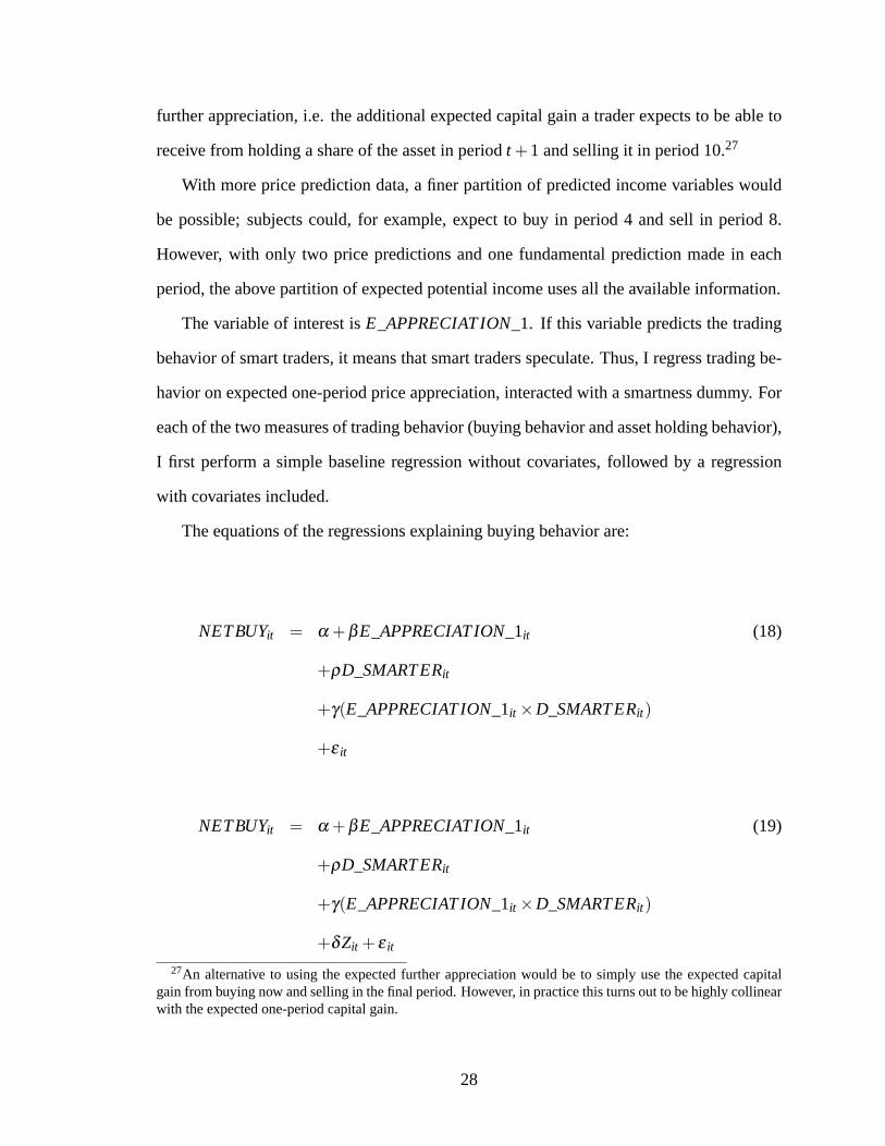
further appreciation, i.e. the additional expected capital gain a trader expects to be able to

receive from holding a share of the asset in period t+1 and selling it in period 10.27

With more price prediction data, a finer partition of predicted income variables would

be possible; subjects could, for example, expect to buy in period 4 and sell in period 8.

However, with only two price predictions and one fundamental prediction made in each

period, the above partition of expected potential income uses all the available information.

The variable of interest is E_APPRECIATION_1. If this variable predicts the trading

behavior of smart traders, it means that smart traders speculate. Thus, I regress trading be-

havior on expected one-period price appreciation, interacted with a smartness dummy. For

each of the two measures of trading behavior (buying behavior and asset holding behavior),

I first perform a simple baseline regression without covariates, followed by a regression

with covariates included.

The equations of the regressions explaining buying behavior are:

NETBUYit = α+βE_APPRECIATION_1it (18)

+ρD_SMARTERit

+γ(E_APPRECIATION_1it×D_SMARTERit)

+ε it

NETBUYit = α+βE_APPRECIATION_1it (19)

+ρD_SMARTERit

+γ(E_APPRECIATION_1it×D_SMARTERit)

+δZit+ ε it

27An alternative to using the expected further appreciation would be to simply use the expected capital

gain from buying now and selling in the final period. However, in practice this turns out to be highly collinear

with the expected one-period capital gain.

28

Where Zit is a vector of covariates that includes:

• CASHi,t−1, the cash in the subject’s account at the beginning of period t,

• SHARESit , the subject’s shares of the risky asset at the beginning of period t,

• E_BUYANDHOLDit , the predicted profit from buying in period t and holding through

the end of the market,

• E_APPRECIATION_Fit , the predicted further price appreciation (i.e., the predicted

capital gain from holding in period t+1 and selling in the final period,

• E_BUYANDHOLDit ×D_SMARTERit , the smartness dummy interacted with the

predicted buy-and-hold value,

• E_APPRECIATION_Fit ×D_SMARTERit , the smartness dummy interacted with

the predicted further price appreciation,

• Pt−1, the lagged average of past asset prices,

• Dt−1, the one-period lagged dividend, and

• t, a linear time trend.

I also run analogous regressions using D_MORECORRECT as the smartness dummy

instead of D_SMARTER.

29

Analogously, the equations of the regressions explaining asset holding behavior are:

ÃSSETSHARE it = α+β ˜E_APPRECIATION_1it (20)

+ρD_SMARTERit

+γ( ˜E_APPRECIATION_1it×D_SMARTERit)

+ε it

ÃSSETSHARE it = α+β ˜E_APPRECIATION_1it (21)

+ρD_SMARTERit

+γ( ˜E_APPRECIATION_1it×D_SMARTERit)

+δZit+ ε it

Where Zit is a vector of covariates that includes:

• ÃSSETSHARE i,t−1

• ÃSSETSHARE i,t−2

• ˜E_BUYANDHOLDit

• ˜E_APPRECIATION_F it

• ˜E_BUYANDHOLDit ×D_SMARTERit , the smartness dummy interacted with the

predicted buy-and-hold value,

• ˜E_APPRECIATION_F it ×D_SMARTERit , the smartness dummy interacted with

the predicted further price appreciation,

• Pt−1,

• Dt−1, and

30

• t.

Again I run analogous regressions using D_MORECORRECT as the smartness dummy

in place of D_SMARTER.

The coefficients that measure short-term price speculation are β and γ . A positive value

for the sum of these coefficients indicates speculation by smart traders.

Table I.8 shows the results for Equations 18 and 19, and Table I.9 shows the results for

Equations 20 and 21. The coefficients β and γ are positive and significant in all specifica-

tions28. γ , the interaction-term coefficient, is about one order of magnitude larger than β

in all specifications. The economic interpretation of the coefficients is as follows: a trader

who understood fundamentals well in all previous periods (including the current period), if

she predicted the price to go up by 20 more yen in the next period, bought about 1-4 more

shares of the asset, or held another 10-25% of her wealth in the risky asset. In contrast, a

trader who did not understand fundamentals bought approximately 0.1-0.4 more shares, or

held another 1-2% of her wealth in the risky asset, for a similar increase in predicted one-

period appreciation.29 Not only does a speculative motive exist, it is substantially stronger

for traders who understand fundamentals than for those who don’t. This may be because

smart traders have more confidence in their price predictions.

The result for β and γ is robust to a large set of alternative specifications, including the

omission of either or both of the other predicted income regressors, the use of lagged or

leading values of smartness dummies, more lags of dividends, lagged values of net buying,

quadratic time trends, and the use of an Arellano-Bond panel GMM estimator instead of

OLS.

28The coefficients β and γ are larger when the covariates are included. This is partly

because E_APPRECIATION_Fit , the expected further appreciation, is negatively correlated with

E_APPRECIATION_1it . If E_APPRECIATION_Fit is omitted as a covariate, β and γ are still larger in

the regression with covariates, but the difference is not as large.29Actually, the difference is not quite as large if we take into account the larger variance of price pre-

dictions among traders who do not understand fundamentals. A predicted 20 yen appreciation is about two

unconditional standard deviations of E_APPRECIATION_1 for smart traders, but only about 2/3 of a stan-

dard deviation for confused traders. Thus, the speculation motive is only about three times as strong for smart

traders, not ten times.

31

Thus, short-term speculation is a substantial motive for traders who understand funda-

mentals. Like Result 1, this is an existence result; the coefficients β and γ are not meant

to measure the total speculation motive, but to provide a lower bound (subjects may also

speculate on their predictions of more long-term price appreciation). The result does not

contradict the finding in Lei, Noussair, and Plott (2001) that laboratory bubbles do not

require speculation, but it shows that speculation nevertheless exists and is significant. Im-

portantly, speculation will tend to prevent smart traders from exerting deflating pressure on

bubbles.

4.4 Effect of past prices on trading behavior

Result 3: Lagged average prices are a significant predictor of trading decisions.

Although subjects in this market do speculate, their predictions of future asset returns

do not explain all of their trading behavior. In the regression results in Tables I.8 and I.9,

lagged average prices emerge as a significant regressor with a coefficient several times as

large as the coefficient on expected one-period price appreciation. This result persists in

all of the alternative regression specifications listed above. This result is consistent with

the broad features of observed trading behavior. Subjects tend to hold or sell the asset in

periods 3-6, when the price is higher than its recent values. They then tend to buy in periods

7 and 8, after prices have begun to decline.

An interesting question is whether smart traders differ from other traders in their use

of lagged prices. To assess whether they do, I run the regression in Equation 19 for

subsamples of smart traders only, using several definitions of "smart". The results can

be seen in Table I.10. For the stricter definitions of "smartness" used in most of this

paper (D_MORECORRECTit = 1 and D_SMARTERit = 1), significance cannot be es-

tablished; however, for looser definitions of "smartness" (D_MORECORRECTit = 1 and

D_SMARTERit = 1), lagged prices emerge as significant. This is perhaps not surprising;

32

because prices do not vary across subjects, the relatively small numbers of subjects who

meet the stricter "smartness" criteria result in this regression having low power. But if

smart traders do indeed trade based on lagged prices, it would explain much of the result

in Section 4.1.4; a broad similarity between trader types would be exactly what one would

observe if the price history itself was a significant factor influencing the asset demands of

all subjects. So although the data are insufficient to conclude that the very smartest traders

trade on lagged prices, they indicate that there is a strong possibility that this is happening.

However, even if smart traders do not trade based on lagged prices, the phenomenon

remains interesting and important, because it provides another mechanism by which price-

to-price feedback can cause bubble-shaped asset mispricings. If traders who observe higher

prices in the past are willing to accept higher prices in the future, temporary overpricings

due to mistakes about fundamentals will grow larger over time. Instead of being corrected

by a learning process, bubbles will be self-sustaining.

Why should average past asset prices predict traders’ decision to buy? Because this

experiment used the same price path for all subjects, it is only possible to conjecture. One

possible explanation might seem to be loss aversion. If prices fall, loss-averse subjects

whose wealth has declined may become risk-loving, buying in the hope that prices will rise

and they will recoup their losses. However, given that most smart traders (as well as most

traders in general) expect positive asset returns in periods 7 and 8, loss aversion seems like

an incomplete explanation. Additionally, loss aversion is unable to explain the substantial

nonzero asset holdings of many smart traders even at the bubble peak.

A second possible explanation is that a trader’s predictions of future prices may depend

on the prices she has observed in the past. Subjects may thus be engaging in a simple

form of technical analysis, in which they try to gauge "support levels." If the market has

demonstrated that it is willing to pay a price of 60 for the asset, and the price falls to 55,

the asset may look "cheap." In fact, lagged average prices are positively correlated with

predictions of future prices, as one would expect if subjects were forming their beliefs in

33

this way. However, this explanation too seems incomplete; even when expectations of final-

period prices are included as regressors, lagged average prices still emerge as significant.

If subjects believed in "support levels," this belief should reflect itself in their final-period

price predictions. Nor does error in the measurement of price predictions seem likely to

explain all of the result, since the coefficient on lagged prices is an order of magnitude

larger than the coefficients on price predictions.

There is a third possible reason for the "lagged price effect": herd behavior. Avery

and Zemsky (1998) define herd behavior in financial markets as occurring when a trader

reverses her trading decision (e.g. buys instead of sells) based on her observation of the

trading decisions of others30. In the present experiment, subjects do not directly observe

the actions of the others, only prices. However, note that observing a market price of 60 yen

conveys the information that there existed subjects in the Source Market who purchased the

asset for 60 or more yen in the given period31. If this observation affects the behavior of

traders in the present study, then herd behavior is present.

Why would traders "imitate" the traders in the Source Market? This would happen

if subjects do not equate the asset’s fundamental value with the dividend income that it

provides. Subjects may feel instinctively that if traders in the Source Market were willing

to pay 60 yen for the asset, the asset must be worth somewhere in the neighborhood of

60 yen, while not explicitly forming beliefs about why it would have this value. "Smart"

traders may understand all of the experimental parameters, yet fail to intuitively grasp that

dividend income and resale value are the asset’s only sources of value (alternatively, they

may understand that dividends equal fundamentals, but not have complete confidence in

this knowledge). While this type of herding would not fit the typical description of rational

information-based herding (see Hirshleifer and Teoh 2001), it would constitute "behav-

30This is similar to the definition of herding given in Bikhchandani, Hirshleifer, and Welch (1992). It is

unrelated to the notion of "managerial herding" in Scharfstein and Stein (1990). Note that the Avery and

Zemsky (1998) also includes the kind of "technical analysis" postulated above; however, since in Avery and

Zemsky’s (1998) highly stylized model, traders are not allowed to resell the asset, I consider "support levels"

and "herding" to be separate notions.31And, additionally, that the traders who bought at 60 were in some sense "average".

34

ioral" or "instinctual" herding.

Such behavior is irrational, but it closely matches a very plausible strategy for real-

world investing. A trader first assumes that the market is basically efficient, and that market

prices are close to "right." She then looks for information that indicates small differences

between the current price and the asset’s true fundamental value or future resale value.

When she is reasonably confident that such a difference exists, she makes a trade. This

type of behavior is entirely consistent with the actions of the individual investors in the

present experiment. However, though this strategy may sound reasonable, it represents

herd behavior. If market prices deviate from fundamentals due to heterogeneous beliefs or

mistakes, lagged asset prices no longer represent a good baseline for valuing an asset.

4.5 Design-experienced traders

Figure I.7 displays average net buying and average asset holdings for Market 2, along with

market prices. The pattern of net buying appears similar to that in Market 1, with strong ini-

tial asset demand, reduced demand in middle periods when prices are most different from

fundamentals, and then a positive spike in demand when prices begin to fall steeply. How-

ever, unlike in Market 1, ASSETSHARE falls steeply as prices fall; this happens because

the fall in prices overwhelms subjects’ after-peak buying.

Repeating the regressions from Equations 18-21 yields results that differ from the re-

sults in Market 1. Beliefs about future prices no longer emerge as a significant predictor of

trader behavior (see Table I.11). The impact of lagged prices in this market is difficult to

assess, since prices in Market 2 are highly collinear with time. When time is omitted from

the regressions, lagged prices become an important explanatory variable (Table I.11);32

however, it is impossible to tell whether this is due to an effect like that seen in Market 1,

or due to a time trend in asset demand.

These results indicate that design-experienced subjects rely less on their price predic-

32This is true even when the sample is restricted to smart traders.

35

tions than do design-inexperienced subjects; speculation is not obviously in evidence. This

is consistent with the smaller incidence of bubbles seen in market repetitions in most asset

pricing experiments.

4.6 Effects of experimental treatments

Table I.12 shows that the number of smart traders (D_SMARTERi,10 = 1) was significantly

higher (p-value=0.004) in the Pictures treatment, and insignificantly lower (p-value=0.134)

in the Uncertain treatment (Wilcoxon rank-sum tests).33 Showing subjects examples of

feasible price and dividend series does increase their understanding of fundamentals, a

result similar to that found by Lei and Vesely (2009).

However, NETBUY and ASSETSHARE are not significantly different across the three

treatment groups in period 7 or period 8 of Market 1 (see Table I.13). The greater un-

derstanding of fundamentals induced by the Pictures treatment does not stop traders from

buying into the bubble after the peak. When the sample is restricted to only smart traders

(D_SMARTERit = 1), smart traders in Treatment 3 are found to buy significantly fewer

shares in period 7 (p-value=0.045). Thus, there is some evidence that the Pictures treat-

ment prevented smart traders from joining the bubble.

To ascertain whether subjects in the different treatments speculated to different degrees,

33This result also holds for D_SMARTi,10. A similar result obtains for the null hypothesis that cumulative

mistakes ∑t Mit are the same across treatment groups; mistakes are insignificantly higher in the Uncertain

treatment and significantly lower in the Pictures treatment.

36

I use the following regressions:

NETBUYit = α+β ×E_APPRECIATION_1it (22)

+ρD_PICTURESi

+γ× (E_APPRECIATION_1it×D_PICTURESi)

+Zit+ ε it

˜ASSETSHARE it = α+β × ˜E_APPRECIATION_1it (23)

+ρD_PICTURESi

+γ× ( ˜E_APPRECIATION_1it×D_PICTURESi)

+Zit+ ε it

Here, D_PICTURESi is a dummy for the Pictures treatment, and Zit is a vector of

covariates34. Analogous regressions were run with D_UNCERTAINi, a dummy for the

Uncertain treatment, in its place. The Uncertain treatment is found to have no measurable

effect on the degree of speculation. The results of the estimations for the Pictures treatment

appear in Table I.14.. Subjects in the Pictures treatment were found to trade significantly

less in accordance with their predictions of one-period price appreciation, and significantly

more in accordance with their predictions of further price appreciation.

This result is perhaps surprising, since subjects who had seen examples of market price

paths had more information with which to speculate. In particular, they could see that prices

tended to display significant momentum, and that prices in bubble markets tended to peak

and decline in the middle of the market. However, these traders chose to speculate less (at

least in the short term) than traders who had no such information. This is contrary to the

result of Haruvy, Lahav, and Noussair (2007), who find that traders who have witnessed

34The covariates are the same as in Equations (*****) and (*****), except with treatment dummies instead

of smartness dummies.

37

bubbles try to "time the market," buying into a bubble and attempting to sell out just before

the peak.

I conjecture that the reason for the decreased speculation in the Pictures treatment is

greater attention to risk. Seeing a large array of different price paths informs subjects of

the potentially large variance of prices, and discourages speculative behavior. This could

also explain the decreased degree of speculation exhibited by all subjects in Market 2; after

having witnessed a rise and crash in prices, and after having traded on their own incorrect

price predictions, traders are more hesitant to trust their own judgment. This explanation

has the flavor of the "overconfidence" literature (e.g. Barber and Odean 2000, Scheinkman

and Xiong 2003), in which individual investors overestimate the precision of their own

forecasts.

5 Conclusion

What can bubble experiments tell us about real-world bubbles? If bubble-shaped mispric-

ings in real-world asset markets are caused primarily by feedback effects between non-

financial sectors and asset markets, then the answer is "little." But if bubbles are caused by

"price-to-price feedback," in which price movements themselves cause later price move-

ments, then it may be possible to increase our understanding of the bubble phenomenon by

studying simple, isolated financial markets like the one presented in this paper. The focus

of "bubble experiments" should therefore be on identifying the behavioral and institutional

sources of price-to-price feedback.

The first main contribution of this paper is to show that price-to-price feedback in simple

experimental asset markets is not purely a function of subject confusion. The tendency of

traders who understand fundamentals to buy just after the peak of a bubble shows that the

movement of prices alone is sufficient to make these "smart" traders knowingly overpay for

a risky asset - behavior that, in equilibrium, will have an effect on the price. This is the first

38

study to show conclusively that this is the case.

This paper’s second main contribution is to identify one source of price-to-price feed-

back, and to present evidence that a second source exists. "Smart" traders tend to trade

based on their predictions of short-term price appreciation, irrespective of their understand-

ing of fundamentals. This form of speculation may not be necessary for bubbles to appear

(as in Lei, Noussair, & Plott 2001), but it clearly has the potential to contribute to bubbles.

If smart traders predict that an already overpriced asset will continue to increase in price

(as they do in Market 1 of this experiment), short-term speculation will tend to reduce the

degree to which these smart traders pop bubbles through arbitrage.

The second source of price-to-price feedback in this experiment is unknown. In this

experiment, subjects were more likely to demand a risky asset at a given price when past

prices had been higher. This indicates the possibility that a form of herd behavior is at

work, in which subjects believe that the market price is "close to right." If further research

shows this to be the case, it will have profound implications for our understanding of how

asset markets function. Generally, we think of markets as aggregating information. But if

price bubbles - initiated, perhaps, due to heterogeneous beliefs or a burst of overconfident

speculation - cause traders to believe that the market price is the "right" price, it means

that financial markets have the capacity to aggregate misinformation. That is clearly a

phenomenon deserving of more study.

The third contribution of this paper is to identify a phenomenon of "after-peak buying."

In this experiment, a group of traders whose net demand was approximately zero at the

peak of a bubble began to buy strongly when the price began to fall. In a market equilib-

rium, this positive net demand would cause the price to rise, and thus sustain or reinflate

the bubble. Although many studies focus on the initial causes of mispricings, another in-

teresting question is why those mispricings are sustained. This question, too, is a goal for

future research.

Finally, this paper makes a methodological contribution to the asset-pricing experiment

39

literature. Whereas most asset market experiments use small markets as their unit of analy-

sis, this study uses non-interacting individual traders facing market prices that they are too

"small" to affect. Although this partial-equilibrium approach is not as useful as the typical

setup for studying the effects of institutions on market outcomes, it is potentially more use-

ful for studying the determinants of individual behavior, since it removes price endogeneity,

group fixed effects, and coordination effects from the analysis. In one regard, this approach

actually has more external validity than the traditional small-market general-equilibrium

setup, since real-world investors are often individually too "small" to affect prices. An-

other way of saying this is that in a traditional asset-pricing experiment individual behavior

is aggregated by a small, illiquid market, while a partial-equilibrium experiment provides

insight into the individual behavior patterns that will be aggregated by large, liquid markets

in the real world.

There are three fairly obvious extensions of this experiment that should be pursued

in order to better understand and extend the results. The first is to vary the price path,

using price series from a number of experimental "source" markets. This will allow a

clearer determination of the effect of past prices on expectations of future prices, as well

as on trading behavior. The second extension is to assess subjects’ willingness to pay

for the asset, using a call market setup. Such a setup would allow a determination of

the size of the mispricing that the most bullish traders would be willing to support for a

given history of prices and dividends. It would also allow computation of the hypothetical

equilibrium price that would emerge from an aggregation of individual trader demands, and

allow the experimenter to compare this price with the pre-determined market price, in order

to ascertain whether traders on average would tend to pop or further inflate a given bubble.

The third extension is to relax constraints on short selling and margin buying, as has been

done in some "group" bubble experiments.

The methodology in this study also has applicability beyond the bubble experiment lit-

erature. The partial-equilibrium approach used here represents an important complement

40

to traditional market-clearing experimental techniques, since it has the capability to isolate

the determinants of individual behavior and expectations. There are any number of ob-

served market phenomena that might be caused by a number of different types of behavior

at the individual level - excess volatility, under-saving, and large equity premia, to name

just a few. Additionally, although the process of individual expectation formation was not

a major focus of this paper, expectation formation under uncertainty is obviously another

area where a partial-equilibrium approach can be of use. These applications should be con-

sidered not only in terms of their relevance to financial economics, but to macroeconomics

in general.

41

42

Tables and Figures

Figure I.1a: Prices and Fundamentals in Market 1

0

20

40

60

80

100

120

1 2 3 4 5 6 7 8 9 10

Yen

Period

Dividend Price

Fundamental Value Maximum Value

43

Figure I.1b: Prices and Fundamentals in Market 2

0

20

40

60

80

100

120

1 2 3 4 5 6 7 8 9 10

Yen

Period

Dividend Price

Fundamental Value Maximum Value

44

Figure I.2: Diagram of the Experimental Procedure

Figure I.3: Confused Traders’ Mistakes About FV in Market 1

0

50

100

150

200

250

300

350

400

1 2 3 4 5 6 7 8 9 10

Yen

Period

Price FV Mistake

45

Fig. I.4a: Price Predictions vs. Lagged Prices, Market 1, All

Subjects

Fig. I.4b: Price Predictions vs. Lagged Prices, Market 1, Smart

Traders

0

50

100

150

200

250

300

1 2 3 4 5 6 7 8 9 10

Yen

Period

Lagged price

Prediction of upcoming period price

Prediction of final period price

0

50

100

150

200

1 2 3 4 5 6 7 8 9 10

Yen

Period

Lagged price

Prediction of upcoming period price

Prediction of final period price

Prediction of fundamental value

46

Figure I.5a: Average Net Buying in Market 1

Figure I.5b: Average Asset Shares in Market 1

0

10

20

30

40

50

60

70

80

-5

-4

-3

-2

-1

0

1

2

3

1 2 3 4 5 6 7 8 9 10

Yen

Shar

es

Bo

ugh

t

Period

All Subjects Smart Traders Price

0

10

20

30

40

50

60

70

80

0

0.1

0.2

0.3

0.4

0.5

0.6

0.7

1 2 3 4 5 6 7 8 9 10

Yen

Frac

tio

n o

f W

eal

th in

Ris

ky

Ass

et

Period


47

Figure I.6a: Average Net Buying in Market 1 (Extreme

Groups)

Figure I.6b: Average Asset Shares in Market 1 (Extreme

Groups)

0

10

20

30

40

50

60

70

80

-8

-6

-4

-2

0

2

4

6

8

10

1 2 3 4 5 6 7 8 9 10

Yen

Shar

es

Bo

ugh

t

Period

Smartest Traders Most Confused Traders Price

0

10

20

30

40

50

60

70

80

0

0.1

0.2

0.3

0.4

0.5

0.6

0.7

0.8

0.9

1

1 2 3 4 5 6 7 8 9 10

Yen

Frac

tio

n o

f W

eal

th in

Ris

ky

Ass

et

Period

Smartest Traders Most Confused Traders Price

48

Figure I.7a: Average Net Buying in Market 2

Figure I.7b: Average Asset Shares in Market 2

0

10

20

30

40

50

60

-10

-8

-6

-4

-2

0

2

4

6

1 2 3 4 5 6 7 8 9 10

Yen

Shar

es

Bo

ugh

t

Period


0

10

20

30

40

50

60

0

0.1

0.2

0.3

0.4

0.5

0.6

0.7

0.8

1 2 3 4 5 6 7 8 9 10

Yen

Frac

tio

n o

f W

eal

th in

Ris

ky

Ass

et

Period


49

Table I.1: Treatments

Day # of Subjects Treatment

1 26 Basic

2 3 Basic

3 20 Uncertain

4 19 Pictures

5 15 Basic

50

Table I.2: Smartness Dummies

# of Traders in Period

Smartness Dummy Definition 1 2 3 4 5 6 7 8 9 10

Prediction of

fundamental is

feasible

57 48 45 42 41 42 36 35 36 39

Prediction of

fundamental is less

than 50% from true

value

36 36 33 30 25 23 27 28 26 39

Prediction of

fundamental is less

than 5 yen from

true value

18 29 15 22 20 20 17 26 26 39

Prediction of

fundamental is

feasible in all

previous and

current periods

57 45 41 38 35 33 31 29 29 28

Prediction of

fundamental is less

than 50% from true

value in all

previous and

current periods

36 27 24 23 17 15 14 14 13 13

Prediction of

fundamental is less

than 5 yen from

true value in all

previous and

current periods

18 13 8 8 6 6 4 4 4 4

51

Table I.3: Price Predictions

LHS: E_PNEXTit

Regressor Coefficient p-value

Pt-1 0.681*** 0.000

Pt-1 – Pt-2 -0.547 0.112

D_MORECORRECTit 0.425 0.777

D_MORECORRECTit*( Pt-1 – Pt-

2) 0.874* 0.059

#obs = 664 R-squared: 0.382

LHS: E_PNEXTit


Pt-1 0.729*** 0.000

Pt-1 – Pt-2 -0.439 0.130

D_SMARTERit 0.914 0.665

D_SMARTERit*( Pt-1 – Pt-2) 0.758** 0.041

#obs = 664 R-squared: 0.349

Note: *** = significant at the 1% level, ** = significant at the 5% level, * = significant at

the 10% level

52

Table I.4: Variation of Price Predictions

Period

Standard deviation of upcoming-period price

prediction as a percentage of market price

1 3.319

2 0.423

3 0.914

4 0.225

5 0.221

6 0.226

7 0.228

8 0.564

9 0.736

10 0.758

53

Table I.5: Net Asset Demand by Period

Period Price Price-FV

(Price-

FV)/FV

Total net

buying

Total net

buying /

shares

outstanding

(%)

p-value for

H0:

1 60 10 1.2 184.9 44.56 0.000

2 56 11 1.2 120.0 20.00 0.000

3 60 20 1.5 -52.0 -7.22 0.191

4 63 28 1.8 27.0 4.04 0.679

5 68 38 2.3 -33.0 -4.75 0.933

6 64 39 2.6 34.0 5.14 0.252

7 58 38 2.9 211.0 30.31 0.000

8 51 36 3.4 124.0 13.67 0.001

9 43 33 4.3 51.0 4.95 0.696

10 31 26 6.2 -326.0 -33.27 0.000

54

Table I.6: Trading Behavior in Periods 7 and 8

Perio

d

Pric

e -

FV

(Price-

FV)/F

V Trader Category

# of

Trader

s

%

who

bough

t

%

wh

o

hel

d

Averag

e net

buying

Averag

e asset

share

7 38 1.9 All 83 71 23 2.54 0.54

7 38 1.9

27 70 19 1.96 0.42

7 38 1.9 14 71 21 1.93 0.36

8 36 2.4 All 83 48 34 1.43 0.59

8 36 2.4

26 50 35 1.86 0.47

8 36 2.4 14 50 29 2.64 0.45

55

Table I.7: Net Buying in Periods 7 and 8

Perio

d

Pric

e -

FV

(Price-

FV)/F

V Trader Category

# of

Trader

s

p-value for

H0:

p-value for

H0:

7 38 1.9 All 83 0.000 0.000

7 38 1.9

27 0.000 0.001

7 38 1.9

14 0.011 0.004

8 36 2.4 All 83 0.001 0.001

8 36 2.4

26 0.029 0.054

8 36 2.4

14 0.071 0.103

p-value for

H0:

p-value for

H0:

7 38 1.9 All 83 0.008

7 38 1.9

27 0.360

7 38 1.9

14 0.488

8 36 2.4 All 83 0.000 0.000

8 36 2.4

26 0.240 0.001

8 36 2.4

14 0.267 0.023

56

Table I.8a: Determinants of Net Buying

LHS: NETBUYit

Simple Regression Covariates Included

Regressor Coefficient p-value Coefficient p-value

E_APPRECIATION1it 0.010*** 0.008 0.010** 0.017

D_MORECORRECTit -0.262 0.284 0.824 0.207

E_APPRECIATION1it ∗

D_MORECORRECTit 0.108*** 0.005 0.099** 0.046

E_BUYANDHOLDit

0.001** 0.013

E_APPRECIATIONFit

0.003 0.516

E_BUYANDHOLDit ∗

D_MORECORRECTit 0.034 0.147

E_APPRECIATIONFit ∗

D_MORECORRECTit 0.04*** 0.000

CASHi,t-1

0.007** 0.011

Dt-1

0.016 0.653

SHARESi,t-1

0.102 0.333

T

-0.375*** 0.007

P-bart-1

0.771*** 0.000

#obs: 747 R-squared: .024 R-squared: .162


the 10% level

57

Table I.8b: Determinants of Net Buying

LHS: NETBUYit



E_APPRECIATION1it 0.010** 0.010 0.012*** 0.005

D_SMARTERit -0.389* 0.086 1.549 0.100


D_SMARTERit 0.138*** 0.003 0.227** 0.010

E_BUYANDHOLDit

0.001** 0.014

E_APPRECIATIONFit

0.004 0.326

E_BUYANDHOLDit ∗

D_SMARTERit 0.075** 0.024


D_SMARTERit 0.034*** 0.002

CASHi,t-1

0.007*** 0.005

Dt-1

0.004 0.900

SHARESi,t-1

0.123 0.231

T

-0.398*** 0.003

P-bart-1

0.722*** 0.000

#obs: 747 R-squared: .030 R-squared: .282


the 10% level

58

Table I.9a: Determinants of Asset Holding

LHS: ASSETSHAREit



Coefficien

t p-value

E_APPRECIATION1it 0.000 0.562 0.001*** 0.002


D_MORECORRECTit 0.009*** 0.000 0.007*** 0.004

E_BUYANDHOLDit

0.000 0.943

E_APPRECIATIONFit

0.000 0.559

E_BUYANDHOLDit ∗

D_MORECORRECTit -0.001** 0.029


D_MORECORRECTit -0.001 0.52

ASSETSHAREi,t-1

0.479*** 0

ASSETSHAREi,t-2

-0.201** 0.025

Dt-1

-0.002 0.165

t

-0.018*** 0.005

P-bart-1

0.027** 0.015

#obs: 664 R-squared: .032

R-

squared: .232


the 10% level

59

Table I.9b: Determinants of Asset Holding

LHS: ASSETSHAREit



Coefficien

t p-value

E_APPRECIATION1it 0.000 0.516 0.001*** 0.001


D_SMARTERit 0.011*** 0.000 0.013*** 0.006

E_BUYANDHOLDit

0.000 0.93

E_APPRECIATIONFit

0.000 0.522

E_BUYANDHOLDit ∗

D_SMARTERit 0.009** 0.042



ASSETSHAREi,t-1

0.46*** 0

ASSETSHAREi,t-2

-0.212** 0.017

Dt-1

-0.003 0.112

T

-0.016** 0.012

P-bart-1

0.029*** 0.005

#obs: 664 R-

squared: .037

R-

squared: .247


the 10% level

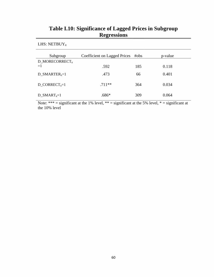
60

Table I.10: Significance of Lagged Prices in Subgroup

Regressions

LHS: NETBUYit

Subgroup Coefficient on Lagged Prices #obs p-value

D_MORECORRECTit

=1 .592 185 0.118

D_SMARTERit=1 .473 66 0.401

D_CORRECTit=1 .711** 364 0.034

D_SMARTit=1 .686* 309 0.064


the 10% level

61

Table I.11a: Net Buying in Market 2

LHS: NETBUYit


E_BUYANDHOLDit 0.001* 0.088

E_APPRECIATION1it 0.003 0.323

E_APPRECIATIONFit 0.006 0.721


E_BUYANDHOLDit ∗ D_SMARTERit 0.0289 0.271

E_APPRECIATION1it ∗ D_SMARTERit 0.0168 0.558

E_APPRECIATIONFit ∗ D_SMARTERit 0.00339 0.923

CASHi,t-1 0.0160*** 0.000

Dt-1 -0.007 0.815

SHARESi,t-1 0.518*** 0.000

P-bart-1 0.586*** 0.000



the 10% level

62

Table I.11b: Asset Holding in Market 2

LHS: ASSETSHAREit


E_BUYANDHOLDit 0.000 0.339

E_APPRECIATION1it 0.000 0.581


E_BUYANDHOLDit ∗ D_SMARTERit -0.003** 0.043

E_APPRECIATION1it ∗ D_SMARTERit -0.000 0.857

E_APPRECIATIONFit ∗ D_SMARTERit -0.010*** 0.002

ASSETSHAREi,t-1 0.586*** 0.000

ASSETSHAREi,t-2 -0.160*** 0.001

Dt-1 -0.005*** 0.000

P-bart-1 0.027*** 0.000



the 10% level

63

Table I.12: Effect of Experimental Treatments on

Fundamental Mistakes

Hypothesis z-score p-value

1.497 0.1344

-2.875 0.004

64

Table I.13a: Differences in Period 7 and 8 Trading,

Uncertain Treatment

Period 7

Trader Category #obs

H0:

H0:

All 83 0.569 0.655

14 0.706 0.533

Period 8

H0:

H0:

All 83 0.740 0.915

14 0.705 0.535

Note: *** = significant at the 1% level, ** = significant at the 5% level, * =

significant at the 10% level

65

Table I.13b: Differences in Period 7 and 8 Trading, Pictures

Treatment

Period 7

Trader Category #obs

H0:

H0:

All 83 0.208 0.324

14 0.045** 0.275

Period 8

H0:

H0:

All 83 0.678 0.172

14 0.217 0.064*


the 10% level

66

Table I.14a: Net Buying, Pictures Treatment

LHS: NETBUYit


E_BUYANDHOLDit 0.001* 0.091

E_APPRECIATION1it 0.039** 0.046


D_PICTURESi -0.789** 0.033

E_BUYANDHOLDit ∗ D_PICTURESi 0.002 0.171

E_APPRECIATION1it ∗ D_PICTURESi -0.025 0.193

E_APPRECIATIONFit ∗ D_PICTURESi 0.008 0.545



the 10% level

Note: Other covariates not shown.

67

Table I.14b: Asset Holding, Pictures Treatment

LHS: ASSETSHAREit


E_BUYANDHOLDit -0.000 0.608

E_APPRECIATION1it 0.004*** 0.005

E_APPRECIATIONFit -0.001** 0.015

E_BUYANDHOLDit ∗ D_PICTURESi 0.0004*** 0.001

E_APPRECIATION1it ∗ D_PICTURESi -0.003** 0.024

E_APPRECIATIONFit ∗ D_PICTURESi 0.001*** 0.003



the 10% level

Note: Other covariates not shown.

68

Appendix I.A: Experimental Instructions

(Note: Instructions that appear in normal type were given in all treatments. Instructions

that appear in highlighted font were omitted from the Uncertain treatment. Instructions

that appear in italics were included only in the Uncertain treatment.)

This is an experiment about decision-making in financial markets. In this experiment, you

will participate in a computerized market, in which you will buy and sell a financial asset,

and make predictions about the asset. The better investment decisions and predictions

you make, the more money you take home, so invest wisely!

The Asset

The asset that you will be buying and selling is computer-generated. It is divided into

“shares.” You can buy and sell these shares individually.

The asset market is divided into 10 “periods.” At the end of each period, each share of the

asset pays an amount of money called a “dividend.” This dividend is the amount of yen

that you get for owning the share. The dividend is random, and is determined each period

by a computerized random number generator. The dividends are the same for all shares,

but different from period to period.

Here are the possible dividends, and the percentage chance of each:

Here are the possible dividends. The dividend probabilities are the same in all periods,

but we will not reveal these probabilities:

Dividend per share Percentage chance

0 50% ??

10 50% ??

69

So if you own 3 shares at the end of Period 6, there is a 50% chance that you will get 30

yen in dividend payments at the end of Period 6, and a 50% chance that you will get 0

yen.

70

Buying and Selling

You will have a computerized cash account and asset portfolio. The cash account

contains your cash. You can use this cash to buy and sell shares of the asset. The asset

portfolio contains your shares of the asset.

Each period, you will see the market price of the asset. You can buy as many shares as

you like at this market price, as long as you have enough cash in your account. For

example, if you have 1000 yen in your account and the market price is 100, you can buy

up to 10 shares. Alternatively, you can sell shares at the market price. You can sell as

many shares as you have in your account. Buying and selling shares does not change the

price. In each period, you can buy or sell shares, but not both.

The market price comes from an earlier experiment. In that experiment, groups of 5 or 6

people (experimental subjects like yourself) traded the asset among themselves. The

average price they paid for the asset in each period became the “market price” that you

see.

In addition to the market price, you will see the “high” and “low”. These are the highest

and lowest prices that were paid for the asset when the market price was determined. You

cannot buy and sell at these prices, only at the market price. However, looking at the high

and low may help you decide how much to buy or sell.

The amount of cash in your account after at the end of each period:

Your cash at the beginning of the period – (# of shares you bought) x (market price) + (#

of shares you sold) x (market price) + (this period’s dividend) x (the number of shares in

your portfolio)

71

At the end of the market, you get to take home all the cash in your account.

72

Predictions

Before each period, you will be asked to predict three things:

1. The market price in the upcoming period

This is your prediction of what you think the market price will be in the period that is

about to start.

2. The market price in the final period (period 10)

This is your prediction of what you think the market price will be in the FINAL period of

the market.

3. The Total Dividend Yield Per Share

The Total Dividend Yield Per Share is the TOTAL amount of dividends that you think

someone would receive from ONE share of the asset, if they bought the share in the

upcoming period and held it until the end of the market. So if you think that someone

who bought 3 shares this period and held them until the end of the market would receive

a total of 300 yen in dividends from those 3 shares, then the Total Dividend Yield Per

Share is 100.

73

The Trading Software

The trading software you will be using is called z-Tree. We will show you how it works.

You will always see the following information at the top of the screen

Period This is the current trading period. If it is between periods, this is

the number of the next period.

Time Remaining This is the time left for you to make your decision.

You will always see the following information in a column on the right-hand side of the

screen:

Cash This shows how much cash you currently have in your account.

Cash is denominated in yen.

Shares This shows how many shares of the asset you currently own.

This is called your “portfolio”.

You will also see the following information in a column on the left of the screen:

Market Price This is the price of the asset. You can buy and sell at this price.

High This is the highest price paid for a share of the asset (by the

people in the market where the price was determined).

Low This is the lowest price paid for a share of the asset (by the

people in the market where the price was determined).

74

On the left hand side of the screen, you will also see two charts:

Price History This shows the market price in each of the previous periods

Dividend History This shows the dividend (per share) paid to holders of the asset

in each of the previous periods

Finally, you will see input boxes. These are the boxes where you make your predictions

and your buying/selling decisions.

75

Appendix I.B: Examples of Market Prices and

Dividends (Pictures Treatment)

Note: Translations appear in text outside pictures.

Example 1 (market price)

Example 1 (dividends)

(total dividend per share received in this market = 30)

015

3045

6075

9010

512

013

515

0

shijo

ukak

aku

0 2 4 6 8 10Round

Rei 1 (shijoukakaku)

01

23

45

67

89

10

11

12

ha

itou

0 2 4 6 8 10Round

(kono shijou no zen-round de uketoru haitou no goukei = 30)

Rei 1 (haitou)

76




040

80

12

016

020

024

028

032

036

0

shijo

uka

kaku

0 2 4 6 8 10Round


01

23

45

67

89

10

11

12

ha

itou

0 2 4 6 8 10Round


Rei 2 (haitou)

77




015

30

45

60

75

90

10

512

013

515

0

shijo

uka

kaku

0 2 4 6 8 10Round


01

23

45

67

89

10

11

12

ha

itou

0 2 4 6 8 10Round


Rei 3 (haitou)

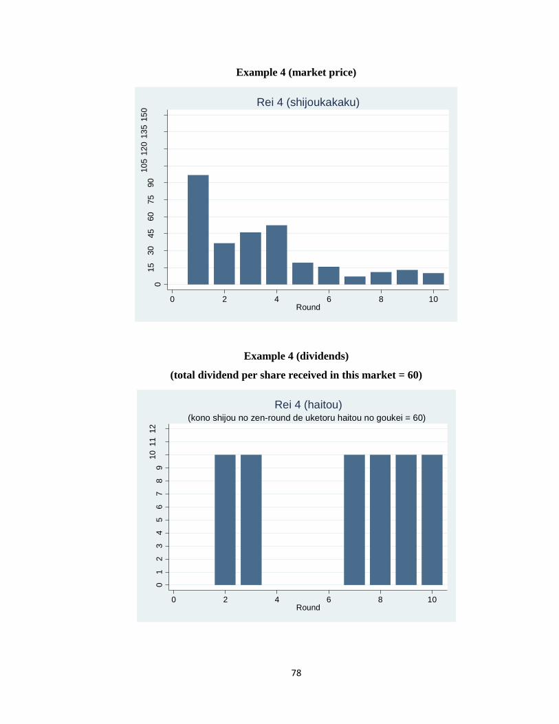
78




015

30

45

60

75

90

10

512

013

515

0

shijo

uka

kaku

0 2 4 6 8 10Round


01

23

45

67

89

10

11

12

ha

itou

0 2 4 6 8 10Round


Rei 4 (haitou)

79

Bibliography

Abreu, Dilip and Markus Brunnermeier. 2003. Bubbles and Crashes. Econometrica

71(1): 173-204.

Ackert, Luck and Bryan K. Church. 1998. The Effects of Subject Pool and Design

Experience on Rationality in Experimental Asset Markets. Working paper.

Ackert, Lucy F., Narat Charupat, Bryan K. Church, Richard Deaves. 2006. Margin, short

sell, and lotteries in experimental asset markets. Southern Economic Journal

73(2): 419–436.

Ackert, Lucy F., Richard Deaves, and Brian D. Kluger. 2006. The origins of bubbles in

laboratory asset markets. Working paper.

Avery, Christopher and Peter Zemsky. 1998. Multidimensional uncertainty and herd

behavior in financial markets. American Economic Review 88: 724—748.

Barber, Brad M., and Terrance Odean, 2000, Trading is hazardous to your wealth: The

common stock investment performance of individual investors. Journal of

Finance 55: 773-806.

Barsky, Robert, 2009. The Japanese bubble: a ‘heterogeneous’ approach. NBER Working

Paper No. 15052.

Bikhchandani, Sushil, David Hirshleifer and Ivo Welch. 1992. A theory of fads, fashion,

custom, and cultural change as informational cascades. Journal of Political

Economy 100(5): 992-1026.

Brunnermeier, Markus and Stefan Nagel. 2004. Hedge funds and the technology bubble.

Journal of Finance 59(5): 2013-2040.

Cagan, Philip. The monetary dynamics of hyperinflation. In Studies in the Quantity

Theory of Money, ed. by M. Friedman. Chicago: University of Chicago Press,

1956.

Caginalp, Gunduz, David Porter, Vernon Smith. 1998. Initial cash/asset ratio and asset

prices: An experimental study. PNAS USA 95 756–161.

Caginalp, Gunduz, David Porter, Vernon Smith. 2000. Momentum and overreaction in

experimental asset markets. International Journal of Industrial Organization 18:

187–204.

80

Caginalp, Gunduz, David Porter, Vernon Smith. 2001. Financial bubbles: Excess cash,

momentum and incomplete information. The Journal of Psychology and

Financial Markets 2(2): 80–99.

DeLong, J. Bradford, Andrei Shleifer, Lawrence H. Summers, Robert J. Waldmann. 1990.

Noise trader risk in financial markets. Journal of Political Economy 98(4): 703-

738.


Positive feedback investment strategies and destabilizing rational speculation. The

Journal of Finance 45 (2): 379-395.

Dufwenberg, Martin, Tobias Lindqvist, Evan Moore. 2005. Bubbles and experience: An

experiment. The American Economic Review 95(5): 1731–1737.

Dwyer, Gerald P. Jr., Arlington W. Williams, Raymond C. Battalio, Timothy I. Mason.

1993. Tests of rational expectations in a stark setting. The Economic Journal 103:

586-601.

Fischbacher, Urs. 2007. z-tree: Zurich toolbox for ready-made economic experiments.

Experimental Economics 10(2) 171–178.

Fisher, Eric. 1998. Explaining bubbles in experimental asset markets. Working paper.

Harrison, J.Michael and David M. Kreps. 1978. Speculative investor behavior in a model

with heterogeneous expectations. The Quarterly Journal of Economics 92(2):

322-336.

Haruvy, Ernan, Yaron Lahav, Charles Noussair. 2007. Traders’ expectations in asset

markets: Experimental evidence. American Economic Review 97(5): 1901–1920.

Hirshleifer, David and Siew Hong Teoh. 2001. Herd behavior and cascading in capital

markets: A review and synthesis. Working paper.

Hussam, Reshmaan N., David Porter, Vernon L. Smith. 2008. Thar she blows: Can

bubbles be rekindled with experienced subjects? American Economic Review

98(3): 924–937.

Kindleberger, Charles. Manias, Panics, and Crashes: A History of Financial Crises, New

York: Basic Books, 1978.

King, Ronald R., Vernon L. Smith, Arlington Williams, Mark V. van Boening, Mark V.

The robustness of bubbles and crashes in experimental stock markets. In R. H.

81

Day and P. Chen, Nonlinear Dynamics and Evolutionary Economics. Oxford,

England: Oxford University Press, 1993.

Kirchler, Michael, Jurgen Huber, Thomas Stockl. 2010. Thar she bursts – a critical

investigation of bubble experiments. Working paper.

Kroszner, Randall. 2010. Implications of the financial crisis. American Economic

Association, Ten Years and Beyond: Economists Answer NSF's Call for Long-

Term Research Agendas. Available at SSRN: http://ssrn.com/abstract=1889315

Lei, Vivian, Charles N. Noussair, Charles R. Plott. 2001. Nonspeculative bubbles in

experimental asset markets: lack of common knowledge of rationality vs. actual

irrationality. Econometrica 69(4): 831–859.

Lei, Vivian, F. Vesely. 2009. Market efficiency: evidence from a no-bubble asset market

experiment. Pacific Economic Review 14(2): 246–258.

Malkiel, Burton. 2010. Bubbles in asset prices. CEPR Working Paper #200.

Morris, Stephen. 1996. Speculative investor behavior and learning. The Quarterly

Journal of Economics 111(4): 1111-1133.

Noussair, Charles N., Stephane Robin, Bernard Ruffieux. 2001. Price bubbles in

laboratory asset markets with constant fundamental values. Experimental

Economics 4: 87–105.

Noussair, Charles N., Steven Tucker. 2006. Futures markets and bubble formation in

experimental asset markets. Pacific Economic Review 11(2): 167–184.

Oechssler, Jorg, Carsten Schmidt, Wendelin Schnedler. 2007. On the ingredients for

bubble formation: informed traders and communication. Working paper.

Porter, David P., Vernon L. Smith. 1995. Futures contracting and dividend uncertainty in

experimental asset markets. The Journal of Business 68(4): 509–541.

Scharfstein, David S. and Jeremy C. Stein. 1990. Herd behavior and investment. The

American Economic Review 80(3): 465-479.

Scheinkman, Jose A., Wei Xiong. 2003. Overconfidence and speculative bubbles.

Journal of Political Economy 111(6): 1183-1219.

Schmalensee, Richard. 1976. An experimental study of expectation formation.

Econometrica 44(1): 17-41

82

Shiller, Robert, 2003. From efficient markets to behavioral finance. Journal of Economic

Perspectives, 17(1): 83-104.

Smith, Vernon, Gerry Suchanek, and Arlington Williams. 1988. Bubbles, crashes, and

endogenous expectations in experimental spot asset markets. Econometrica,

56(5): 1119–1151.

Smith, Vernon, Mark van Boening, Charissa P. Wellford. 2000. Dividend timing and

behavior in laboratory asset markets. Economic Theory 16: 567–583.

Van Boening, Mark, Arlington W. Williams, Shawn LaMaster. 1993. Price bubbles and

crashes in experimental call markets. Economic Letters 41(2): 179–185.

Chapter II

Private Information and Overconfidence in an

Experimental Asset Market

1 Introduction

Trading in financial markets naturally involves an adverse selection problem. If you buy

an asset at a price of x, your counterparty’s willingness to sell at that price indicates that

she may have private information that indicates she is getting the better end of the deal.

If traders ignore this adverse selection, they will tend to engage in suboptimal trades. A

growing body of empirical research supports the hypothesis that traders trade too much.

Odean (1999), for example, finds that excessive trading lowers the returns that individual

investors receive on their portfolios, even when controlling for liquidity and timing de-

mands. Odean’s proposed explanation for this over-trading is overconfidence - the tendency

for investors to believe, incorrectly, that their information is of superior quality to that of

their counteraparty. That sort of belief would lead traders to ignore the adverse selection

problem - if you and I both believe that our information is superior to the other’s, then we

may trade even though we both know we disagree. For this reason, economists have con-

structed a number of models in which trading and asset pricing are driven by overweighting

of private signals about asset fundamentals - i.e., an incorrect but dogmatic belief of each

agent that her own private signals are more precise than those signals really are (and more

precise than the signals of others).

83

This modeling assumption is typically motivated by a large psychology literature on

individual overconfidence. Psychologists have shown that people tend both to overestimate

the precision of their own information ("miscalibration" about signal precision) and to be-

lieve that they are above average in ability (the "better than average effect"). Both of these

effects could cause the overweighting of private information in financial markets.

So behavioral theories of overtrading posit a two-step chain of causality: Psychological

overconfidence –> Overweighting of private information –> Market outcomes. Experi-

mental and empirical tests of these theories, however, have focused only on the direct link

between overconfidence and market outcomes. In this paper, I use an experiment to disen-

tangle the two steps in the causal chain; in other words, I ask two questions:

1. Do traders trade based on ex ante symmetric private signals of asset fundamentals?

2. Do more overconfident traders rely more on private signals to make trading deci-

sions?

To answer these questions, I use a variant of the most common laboratory financial mar-

ket setup (Smith, Suchanek, and Williams 1988), where groups of subjects trade a single

risky asset in three successive fixed-horizon markets. In my experimental markets, traders

receive noisy private signals of asset fundamentals. They also make predictions about the

future path of asset prices. Before trading begins, I use a Bayesian inference task to gauge

two types of individual overconfidence commonly cited in the behavioral finance literature

- miscalibration about signal precision, and the "better than average effect." This task is a

signal-extraction problem that is extremely similar to the one by which dividends can be

inferred from forecasts during the asset market.1 On average, subjects are overconfident

1The only difference between the two signal-extraction problems is the probability distribution itself. The

overconfidence test has signals that are less precise than the dividend forecasts in the market. This was done

so that if the similarity between the tasks gave subjects any bias regarding the precision of the dividend

forecasts, that bias would be toward thinking dividend forecasts were less precise, not more precise, than they

actually were.

84

according to both of these measures; also, the two measures are somewhat correlated at the

individual level.

I find that traders do trade based on private information; traders who get better-than-

average forecasts tend to be buyers, while traders who get worse-than-average forecasts

tend to be sellers. This is true even after most trades in a period have been concluded. Also,

asset buyers’ inferred reservation prices depend on their signals to a greater than optimal

degree. These findings are consistent with the modeling approach used in overconfidence-

based models.

However, I find only mixed evidence that the overuse of private information is caused by

psychological overconfidence. Traders who are miscalibrated, or who consider themselves

"better than average" guessers of the random processes underlying their private signals, are

no more likely than others to use their signals to make trading decisions. On the other hand,

miscalibrated traders may set their reservation prices more in accordance with their signals

than do other traders.

Since I have data on overconfidence and on market outcomes, I revisit the direct link be-

tween psychological overconfidence and market outcomes. I find that overconfident traders

do not trade more, and actually may earn higher profits than other traders. When evaluating

aggregate outcomes across market trading groups, my sample size is very small; however,

I observe an apparent correlation between trading volume and the average "better than av-

erage effect" of a trading group. However, I find no such relationship between aggregate

confidence and either asset overpricing or price volatility.

Thus, I find only mixed evidence to support the link between psychological overcon-

fidence and the kind of market phenomena that overconfidence is generally invoked to

explain. Since my overconfidence measures are highly specialized, it may be that other

measures work better to explain aggregate outcomes. However, it is clear that psycholog-

ical overconfidence on signal-extraction tasks does not explain the use of private signals

that I observe in this experiment.

85

My findings also have an interesting implication for the "bubble experiment" literature

that follows Smith, Suchanek and Williams (1988). Use of private information does not

disappear, and actually strengthens, over successive repetitions of the asset market. This

is in stark contrast to the behavior of asset bubbles, which typically disappear by the third

repetition. By focusing on bubbles, asset pricing experiments may be ignoring a more

enduring source of market inefficiency.

Section II reviews the relevant experimental literature, the literature on overconfidence-

based theories of asset markets, and some psychological literature on overconfidence. Sec-

tion III describes the experimental procedures for the market and for the overconfidence

tests. Section IV motivates and states the hypotheses linking the experiment to existing

models of overconfidence. Section V presents and discusses the results of the experiment.

Section VI concludes.

2 Related Literature

2.1 Overconfidence models

Overconfidence models typically attempt to explain one or more of three phenomena: over-

pricing of financial assets, overtrading (or high volume during periods of overpricing), and

excess price volatility.

The first theories of asset markets that could reasonably be called "overconfidence mod-

els" are models of heterogeneous beliefs. In the seminal paper of Harrison and Kreps

(1978), traders have different beliefs about future asset fundamentals, which do not dis-

appear over time; furthermore, these traders "agree to disagree," disregarding the beliefs

of other traders who disagree with them, even though these differing beliefs are known to

all. In this model, in which short selling is not possible, asset values exceed even the most

optimistic traders’ beliefs about the fundamental, since assets also have an option value; as

beliefs fluctuate, assets can be sold and resold at a profit. This option value turns out to be

86

a common result in overconfidence models.

Some later models, such as that of Morris (1996), relax the assumption that agents

are dogmatic in their differences of opinion, allowing traders to learn over time. Because

learning takes time, results similar to that of Harrison and Kreps (1978) occur in the interim.

Another strand of model posited the existence of "noise traders" who do not trade based

on fundamentals; the classic model of this type is DeLong, Shleifer, Summers, and Wald-

mann (1990). These models typically leave noise traders unmodeled, but the modelers

conjecture that noise traders might believe in spurious information about fundamentals.

Beginning in the late 1990s, a number of models attempted to unify the idea of hetero-

geneous beliefs with the psychological literature on overconfidence. These papers mod-

eled overconfidence as a trader’s incorrect, persistent belief that the precision of his own

private signals about asset fundamentals is higher than it really is. One such model is

Odean (1998), in which price-taking traders trade a single risky over a limited time hori-

zon, while receiving private signals about the future payoff of the asset. Although traders

in this model can infer the average private signal from the market price, they place exces-

sive weight on their own signal, so that they value the asset differently than the market.

This generates excessive trading relative to a rational-expectations equilibrium, and results

in prices that exceed fundamentals. However, because short selling is allowed, this model

does not generate overpricing via an option value; overconfidence causes prices to deviate

from fundamental value, but the direction of the deviation is not determined.

A second model along these lines is Scheinkman and Xiong (2003). In this model,

traders trade over an infinite horizon, receiving signals in continuous time. Although the

signals are public knowledge, each trader thinks of one of the signals is his "own" sig-

nal. All signals are actually worthless, but each trader believes that his own signal (and

no other) is correlated with innovations to the asset’s payoff. This model is similar in

spirit to Harrison & Kreps (1978), except that instead of stubbornly disagreeing about the

process governing asset fundamentals, traders disagree only "agree to disagree" about the

87

informativeness of the various signals. Again, with short selling impossible, option value

creates a "bubble,"2 in which prices exceed any trader’s expectation of fundamentals. Also,

heterogeneous beliefs lead to excess volume and excess volatility.

Other, similar "behavioral" models of overconfidence proceed along similar lines. Daniel,

Hirshleifer, and Subrahmanyam (2001) obtain similar results for a portfolio of many secu-

rities. Daniel, Hirshleifer, and Subrahmanyam (1998) model overreaction and underre-

action to news about fundamentals as functions of slowly changing overconfidence and

self-attribution bias. Gervais and Odean (2001) also model overconfidence that changes

due to self-attribution bias. Hirshleifer and Luo (2001) model how overconfident traders

can survive in a market filled with traders with differing levels of confidence, without being

competed out of the market.

2.2 Psychology literature on overconfidence

Several types of overconfidence have been found in psychology experiments. Two receive

special attention in the behavioral economics literature. The first is miscalibration, in which

people are found to overestimate the precision of their knowledge (Lichtenstein, Fischhoff,

and Phillips 1982, Yates 1990). This is typically measured with a confidence interval test:

subjects are asked a number of questions, and along with their answers they are asked to

give a self-predicted confidence interval (usually a 90% confidence interval). If fewer than

90% of their answers lie within the predicted intervals, subjects are said to be miscalibrated.

The second type of overconfidence is the better-than-average effect, which documents that

most people see themselves as better than average in ability (Taylor and Brown 1988, Sven-

son 1981). This is usually measured by asking people if they are better than the average

at some task, e.g. driving a car. If more than 50% claim to be better than average, it sig-

2Note that this model does not generate a runup-and-crash in asset prices; thus, it does not generate a

"bubble" in the sense of the experimental literature reviewed here.

88

nals that overconfidence exists in the population.3 Many studies find that overconfidence

is prevalent among the population; however, on tasks that are easy or repetitive, people

may be well-calibrated or even underconfident (Pulford and Colman 1997, Kahneman and

Riepe 1998).

2.3 Empirical studies

Odean (1999) examines data on individual investor portfolios provided by a discount bro-

kerage. They find that stocks sold by individual traders tend to subsequently outperform

stocks bought by these traders; in other words, individual investors lose money by trading

too much. Odean attempts to control for liquidity demands, tax-loss selling, rebalancing,

and changes in risk aversion, and finds that once these factors are controlled for, over-

trading lowers individual investor returns by an even greater amount. Barber and Odean

(2001) find that this over-trading is correlated with gender; men trade more and thus per-

form worse than women. Since men are often found in psychology experiments to be more

overconfident about their abilities than women, this may be evidence in support of the

overconfidence hypothesis.

Glaser and Weber (2003) test the relationship between individual investor confidence

and trading activity. Using a questionnaire distributed to a large number of investors,

they measure miscalibration (using self-reported confidence intervals) and the better-than-

average effect (using self-reported evaluations of investing skills). They find that miscal-

ibration is not correlated with trading volume, but that the better-than-average effect is

positively correlated with trading volume.

3Of course, the fact that an individual considers himself to be better than average does not mean that

individual is overconfident; she may simply have good information that she is, in fact, better than average.

89

2.4 Asset market experiments

The classic asset market experiment is the "bubble experiment" of Smith, Suchanek, and

Williams (1988) (henceforth "SSW"). In that experiment, small groups of subjects traded

a single short-lived risky asset that paid a stream of dividends. Even though the dividend

process was made public to all traders, the outcome was a large bubble, in which the price

of the asset diverged strongly from the fundamental value and then crashed at the end of the

market. This bubble was accompanied by high trading volume at the peak. When the same

group of subjects repeated the market several times, the bubble progressively shrank and

eventually disappeared; in other words, the outcome approached a rational expectations

equilibrium as subjects became more experienced. This result has become the most widely

replicated result in experimental finance; in the next two decades, bubbles were shown to

be robust to many changes in market institutions and asset fundamentals (King et al. 1993).

Because this market setup is so well-studied, I use it in the present experiment.

The experiment most similar to the one in this paper is the one run by Kirchler and

Maciejovsky (2002). These authors use a setup similar to SSW, but with several modi-

fications. First, traders are asked to predict the price of the risky asset in the upcoming

period. Second, traders receive signals about the other traders’ average predictions. Third,

traders are asked to give confidence intervals about their price predictions. The authors use

the confidence intervals to measure overconfidence (miscalibration). They find that traders

are generally well-calibrated at the beginning of the experiment, but become more over-

confident as they make successive predictions.4 Interestingly, Kirchler and Maciejovsky

find no correlation between overconfidence and trading volume, although they do find that

overconfident traders earn less on average. The authors do not test the relationship between

overconfidence and use of private information.

Other experiments use market setups quite different from the SSW setup. Deaves,

4However, using a second measure of confidence relying on traders’ subjective certainty about their pre-

dictions, the authors find that subjects are often well-calibrated or even underconfident.

90

Luders, and Luo (2003) use twelve single-period markets, where endowments are reset at

the beginning of each market, and payoffs occur at the end of the market. The authors give

traders i.i.d. signals of fundamental value, but deceive their subjects by telling them that the

signals’ precision is correlated with subjects’ performance on a general knowledge ques-

tionnaire. They measure overconfidence by asking subjects to give subjective confidence

intervals on the questionnaire. The authors find that overconfidence (positive miscalibra-

tion) is positively correlated with trading volume. They also find a positive relationship

between miscalibration and the "better than average" effect, as measured by subjects’ self-

predicted rankings of total profits.

Biais et al. (2005) use a trading setup with asymmetric information about asset funda-

mentals, measuring overconfidence (miscalibration) with a confidence interval task. They

find no significant relationship between miscalibration and trading volume, although they

find that miscalibrated subjects earn lower profits.

Finally, a very interesting experiment by Hales (2009) investigates the closely related

question of whether traders "agree to disagree" about the value of an asset. In his experi-

ment, subjects trade in pairs and receive private signals about asset value. Hales finds that

whether traders are prompted to consider the adverse selection problem has a strong effect

on whether trade occurs. When traders are asked to guess the difference between their own

signal and the signal of the other trader, trade tends not to occur; however, without such

prompting, trade does tend to occur. This result suggests that over-reliance on private in-

formation is not due to traders "agreeing to disagree," but simply to their failure to consider

the fact that others have information that may disagree with their own. Hales calls this

effect "myopia"; it is also sometimes called "availability bias."

2.5 Differences from previous literature

The present experiment differs from the existing literature in several ways. First, it directly

tests agents’ use of private information about fundamentals. Traders in this study receive

91

private signals about asset payouts, of a form very similar to the type of signals in models

like Odean (1999). Unlike in previous experiments on overconfidence, this information is

both ex ante symmetric, and contains only information about fundamentals.5

Second, this experiment is the first to measure overconfidence using a test that is ex-

tremely similar to the signal-extraction problem faced by traders in the actual asset mar-

ket. In the psychology literature, "overconfidence" is measured by many different types of

tasks, and there are often large discrepancies between these measures. The present study

attempts to control for these possible sources of systematic error by using the same task for

the confidence test and the asset market.

Third, this experiment uses a market setup - the "bubble experiment" or SSW setup -

that is known to almost always converge to a rational expectations equilibrium by the third

market repetition.

Fourth, this study measures confidence using a task that is very unlikely to be subject to

overconfidence. The signal-extraction task used here is repetitive and simple, and feedback

is swift - all characteristics that are found to be less conducive to overconfidence (Kirchler

and Maciejovsky 2002). Thus, any observed overconfidence on this task probably repre-

sents a lower bound on the degree to which a subject overestimates her own predictive

accuracy and relative performance.

3 Experimental Setup

3.1 Subjects and compensation

The experiment was conducted on four days, between May 29 and June 7, 2012, at the

Institute for Social Research at the University of Michigan. Subjects were de-identified, so

5Some financial market experiments have established the result that markets aggregate information that

is distributed among different traders (Plott and Sunder 1988). However, these experiments have typically

not given subjects noisy information, and have typically not examined whether subjects’ individual behavior

reflects an underestimation of the amount of noise in their own information relative to the noise in others’

information.

92

no individual data is known except that all were over 18 years old. The majority of subjects

were probably undergraduate students at the University of Michigan. On each day, there

were 12 experimental subjects in the lab, divided into two trading groups of 6 subjects

each. Data from six trading groups are excluded from the analysis due to procedural errors

by the experimenters, so that there are a total of 36 subjects in the sample.6 The entire

experiment lasted approximately two and a half hours. Ex ante average compensation7 was

$38, including a $5 show-up fee. Realized average compensation over the five days was

$35.79. This is in line with the typical per-hour compensation for this type of experiment.

Compensation was divided among the preliminary tasks and the financial market itself, as

will be explained in the following subsections. Payment for all parts of the experiment was

given in cash at the end of the Asset Market portion of the experiment.

3.2 Experimental procedures

The instructions for the experiment are presented in Appendix II.A. The experiment con-

sisted of four parts:

1. A financial literacy test

2. A time-series prediction task

3. A confidence test

6One of the 6 excluded groups was excluded because in Round 1, subjects in the group exhibited a strong

tendency to trade against their forecasts; subjects with better forecasts strongly tended to sell in this round,

while subjects with worse forecasts strongly tended to buy. It was thus inferred that this group was subject

to an error on the part of the experimenters - either a coding error that reversed the displayed forecasts, or

possibly an error by the experimenters when explaining the "bullish" vs. "bearish" terminology. This may at

first appear to represent "cherry-picking" of the data on the part of the experimenter. However, inclusion of

this group in the sample does not in any way alter the result that, across all groups, traders strongly tended

to buy when they received better forecasts and sell when they received worse ones (Hypothesis 1); in fact,

the result is strengthened for Round 3. Also, the results on overconfidence are not altered (and the positive

results are actually strengthened) by the inclusion of this group. Hence, exclusion of this group on the basis

of an inferred experimenter error does not represent cherry-picking of the data to support the experimental

hypotheses.7Since some compensation depended on the accuracy of subjects’ price predictions during the financial

market, the $38 estimate was to some degree a guess on the part of the experimenter, based on trial runs of

the experiment.

93

4. The asset market itself

The purpose of the financial literacy test and time-series prediction task was twofold:

A) to measure subjects’ basic competence (since nothing was known about the subjects’

experience or ability), and B) to induce exogenous variation in group confidence levels. For

this reason, the test and the time-series prediction task were administered in two different

versions, an "easy" version and a "hard" version (subjects were not told that two versions

existed). The differences between these versions will be explained later. Unfortunately,

however, the different versions failed to induce measurable differences in confidence, as

will be explained later. The version of the preliminary tasks received by each trading group

is displayed in Table II.1.

All portions of the experiment were carried out using the z-Tree software package (Fish-

bacher 2007).

3.3 Financial literacy test

The first portion of the experiment was a five-question financial literacy test. This test was

based on the literacy test in Rooij, Lusardi, and Lessie (2011). The "easy" version of the

test consisted of the five "basic literacy questions" created by Rooij et al., while the "hard"

version of the test consisted of five of the eleven "advanced literacy questions." The text of

these questions is given in Appendix II.C. Subjects were given one minute to answer each

question, and were told the correct answer after answering each question.

Each subject received $2 for taking the financial literacy test, regardless of score.

3.4 Time-series prediction task

The second portion of the experiment was a "prediction task". Subjects were asked to pre-

dict the future value of a time series (labeled "GDP") from past values of the time series,

using no other information other than the series’ past values. The time series was gen-

94

erated before the experiment by an AR(1) process with Gaussian white noise innovations

and a linear time trend. At the beginning of the task, subjects were shown a pre-existing

ten-period "history" of the time series, which they used to make their first one-period-

ahead prediction. After each prediction, the realized value of "GDP" for the next period

was revealed, along with the subject’s prediction error; subjects would then make another

one-period-ahead prediction, while seeing the initial ten-period history and all subsequent

realizations of the time series. Each subject made ten predictions in all. At the end of the

task, the subject was told their total prediction error.

The "easy" version of the time series had higher persistence and a smaller variance of

the innovation term than the "hard" version; the time trends were the same. The values of

the "easy" and "hard" time series are listed in Appendix II.D.

Each subject received $2 for completing the prediction task, regardless of score.

3.5 Confidence test

The confidence test was presented to the subjects as "Prediction Task 2". In this task,

subjects were asked to guess whether a pair of "balls" was drawn from "Jar A" or "Jar B".

Each ball was identified by its color; these colors could take on five values, red, orange,

yellow, green, and blue. Subjects were told the number of balls of each color in Jar A and

Jar B, respectively. Each subject made 15 guesses; the number of balls of each color in

each jar did not change between guesses, indicating that the draws were i.i.d. The number

of balls of each color in each jar are listed in Table II.2.

Subjects were not told whether their guesses were right or wrong. After making 15

guesses, subjects were asked to predict how many correct guesses they had made (out of

a possible 15). They were also asked to predict their rank among the 12 subjects in the

lab on that day, so that a rank of 1 would indicate that a subject made as many or more

correct guesses than any other subject in the lab. Even after making these guesses, subjects

were not told how many correct guesses they had made, or their true rank. These two

95

self-predictions were used to generate the two confidence measures used in the experiment.

The difference between a subject’s guess of his or her number of correct answers and the

true number he or she got correct is defined as that subject’s "miscalibration" about signal

precision, while a subject’s predicted ranking defines his or her "better than average effect"

(or "BOA").

This task was a simple Bayesian inference task. It was essentially identical to the

problem of guessing the true per-period dividend from a private forecast during the asset

market (see next subsection), though the probabilities were different. This is important,

because individuals may have different levels of confidence for different types of tasks. An

individual’s confidence on a Bayesian prediction task may be a good or a poor proxy for

her confidence on, say, a market-timing task. To my knowledge, this experiment is the first

to measure confidence using the same kind of signal-extraction problem that is required of

traders in the asset market.

3.6 Asset market

The asset market portion of the experiment closely follows the setup of Smith, Suchanek,

and Williams (1988). Each market consisted of a trading group of 6 subjects. The assets

traded included one riskless asset ("cash," measured in "yen"), and one risky asset (called

simply "the asset," measured in "shares").

Each group of subjects traded over three market rounds. The subjects in each group

were the same from round to round. At the beginning of each market round, each subject

was given an initial endowment of cash and shares. There were three types of endowments,

each with identical ex-ante value; in each market, two traders in each group received Type

1 endowments, two received Type 2 endowments, and two received Type 3 endowments;

the allocation of endowments was randomized given this constraint.

Each market round included ten two-minute trading periods. During a period, subjects

could buy and sell the asset from each other. At the end of a period, each share of the

96

asset paid a dividend to its holder; this dividend was either 0 yen or 10 yen, with a 50%

probability of each. Dividends were the same across all shares within a period, but different

from period to period and different across groups. Dividends were i.i.d. At the end of each

period, traders were told the realized dividend for that period, and the appropriate dividend

income was added to traders’ cash accounts8. After the final dividend was realized at the

end of Period 10 in each round, the asset vanished (no buyout value).

At the end of a market round, subjects received the promise of an amount of cash equal

to the amount of cash in their account, to be paid after the end of the experiment. The

exchange rate was 1 "yen" = 1c/. Thus, there was no "carry-over" between rounds; whatever

a subject earned or did during Round 1 could not affect his or her expected payoff in Round

2 or Round 3.

Trading was done via continuous double auction with an open order book. Each subject

was able to enter bids or asks, or to accept the best available bid or ask. In addition, to

facilitate rapid trading, any subject could press a button that submitted a bid (ask) that

was 1 yen higher (lower) than the highest (lowest) available bid (ask). Shares could only

be bought and sold one at a time. During trading, subjects were told the "buy-and-hold

value" of their current portfolio of risky asset shares; this was equal to 5 yen multiplied

by the number of periods remaining, multiplied by a subject’s number of shares. In other

words, this "buy-and-hold value" was equal to the ex ante risk-neutral fundamental value

of the asset. However, this value did not include the information in subject’s forecasts (see

following subsection).

3.6.1 Forecasts

At the beginning of each period (before the start of trading), each subject received a fore-

cast (noisy signal) of that period’s dividend value. There were five possible forecasts:

"extremely bullish," "moderately bullish," "neutral," "moderately bearish," and "extremely

8Thus, the cash/asset value ratio of the market as a whole increased each period.

97

bearish." Forecasts were i.i.d. across subjects. The probabilities of receiving the different

forecasts were different depending on the different upcoming (but not yet observed) divi-

dend realization; for example, if the dividend was to be 10 yen, the probability of a subject

receiving an "extremely bullish" forecast was 35%. Subjects were given a hard copy of a

chart telling them these conditional probabilities; guessing the dividend from the forecast

was thus a matter of Bayesian inference, identical in form to the guessing task in the earlier

Confidence Test. The forecast probability chart can be seen in Appendix II.B.

Henceforth, to avoid confusion, the term "forecasts" will be reserved exclusively for

these dividend forecasts, while traders’ own predictions of future asset prices (described in

the next subsection) will be referred to only as "predictions."

3.6.2 Price predictions

Before trading in each period, subjects were asked to predict the future average trading

price of the risky asset. Specifically, they were asked to predict:

1. the price in the upcoming trading period, and

2. the price in the final period of the round (Period 10).

Subjects were paid for making accurate predictions, according to an absolute deviation

formula with a minimum of zero. Specifically, for each of the two price predictions in each

period, a subject received a payment equal to max(10 yen−|predicted value−actual value| ,0).

Thus, perfect predictions in all periods in all three rounds would yield a total payment of

600 yen, or $6.9

As mentioned above, the term "predictions" will be reserved for these price predictions,

while the term "forecasts" will be reserved exclusively for the dividend forecasts.

9It is theoretically possible for subjects to intentionally make predictions that are not unbiased functions

of their actual beliefs, even given this symmetric loss function. This would occur if subjects attempt to

make market-timing bets, e.g. betting that the price will go up, but predict a lower price for the purpose of

hedging. However, previous studies, such as Haruvy, Lahav, and Noussair (2007) indicate that such behavior

is negligible in these experiments.

98

3.6.3 Control group

One group (Group C) was not shown any forecasts. This group will be referred to as the

"control group."

4 Theory and Hypotheses

4.1 Overconfidence measures

In the behavioral finance literature on overconfidence, two psychological phenomena - mis-

calibration, and the better-than-average effect - are commonly used to motivate the agents’

overweighting of private signals. However, it is not clear that either one of these phenom-

ena, by itself, is a necessary or sufficient condition for overweighting of private signals.

To see why, let’s examine the model of Odean (1998), which is most similar to the setup

used in the present experiment. In Odean’s model, each agent is aware of the existence

of multiple pieces of noisy information, including the trader’s own private signal of asset

payouts, and other traders’ private signals. The agent’s belief about the precision of each

of these signals differs from the true value. The behavioral multiple that an agent assigns

to his belief about the precision of his own signal is called κ and is assumed to be greater

than or equal to 1, meaning that agents believe that their own signals are more precise than

they really are. The multiple that agents assign to the signals of others is called γ , and is

both assumed to be less than or equal to 1, meaning that agents believe that other agents’

signals are less precise than they really are.

However, in this experiment, it cannot be assumed a priori that these sign restrictions

hold. Suppose a subject demonstrates miscalibration on a test. It may be that this person

overbelieves in the precision not just of her own signals, but of all signals; in other words,

that κ = γ > 1. In the Odean (1998) model, this would cause traders to have common

beliefs, which, given Odean’s other assumptions about preferences would preclude trade

99

after the first period10 and reverse many of the results of the model. Similarly, suppose

a subject demonstrates that he or she believes him or herself to be better than average.

It may be that this person underbelieves in the precision of her own signals, and simply

underbelieves even more in the precision of other signals; in other words, γ < κ < 1. This

is a general problem with these overconfidence measures, and not specific to the Odean

(1998) model, which is used simply to illustrate the point. It is possible that either or both

of these observable confidence measures is a good proxy for the overweighting of private

signals, but this is not guaranteed.

Therefore, when testing hypotheses about the effects of overconfidence, I use three

measures. The first are miscalibration and the better-than-average (henceforth "BTA") ef-

fect, as measured by the two parts of the confidence test described above:

MISCi ≡ self-predicted # of correct guesses - # of correct guesses (1)

BTAi ≡ 6.5 - self-predicted rank (2)

The third is a dummy variable, D_CONFi, equal to 1 if a subject both is positively mis-

calibrated and predicts that she is better than average (and zero otherwise). In other words,

this dummy is 1 when a subject is overconfident according to both common psychological

measures:

D_CONFi ≡

1 MISCi > 0,BTAi > 0

0 otherwise

(3)

Note that if MISCi and BTAi are increasing functions of κ−1 and κ− γ in the Odean

(1998) model, respectively, then D_CONFi = 1 is sufficient to preserve all relevant results

of that model (proof omitted); again, this is for illustrative purposes only, since the ex-

10Odean (1998) allows for traders to have different endowments; after a point of Pareto optimality has been

reached, trade only occurs due to overweighting of the private signals that subsequently arrive.

100

periment is not an exact test of this or any other existing model. In most of the analysis,

I examine only miscalibration and BTA; however, in one or two cases, D_CONFi yields

slightly different results.

4.2 Use of private signals

The first question this paper seeks to answer is: Do traders overweight private signals when

they make their trading decisions? This is the mechanism by which models of heteroge-

neous beliefs generate market inefficiencies. It is also the mechanism by which behavioral

models like Odean (1998) and Scheinkman and Xiong (2003) assume psychological over-

confidence to operate.

A necessary condition for the interaction of individual overconfidence with private sig-

nals is that traders make use of private signals at all. In other words, the dividend forecasts

traders receive in the asset market must cause trades that would not otherwise have oc-

curred. Within a trading group within a period, the distribution of forecasts is i.i.d. Thus,

if traders do not use their forecasts to decide whether to buy or to sell, the probability of

the buyer getting a forecast of 2 (the best possible) and the seller getting a forecast of -2

(the worst) is the same as the probability of the buyer getting a forecast of -2 and the seller

getting a forecast of 2.

Hypothesis 1: The average spread between the dividend forecasts of the buyer and

seller in concluded transactions will be positive.

Use of private signals to make trading decisions does not necessarily imply that traders

overweight these private signals. Because traders may have different risk preferences, ad-

verse selection does not necessarily preclude conditioning trading decisions on private sig-

nals. However, note that if public information in the market - the price, the history of trades,

and the history of orders - reveals the distribution of private forecasts, then trading deci-

sions should not be conditioned on forecasts if rationality is common knowledge. Many

experiments, for example Plott and Sunder (1988), have found that experimental markets

101

with a small number of participants are capable of aggregating private signals about asset

value. Therefore, the finding that subjects in the present experiment condition their actions

on their forecasts will provide stronger support for overweighting of private signals if the

finding holds even after a number of trades have taken place. For this reason, I re-test

Hypothesis 1 for various restricted samples of "late" trades, as described in Section 5.2.

4.3 Private signals and overconfidence

The second question this paper seeks to answer is whether psychological overconfidence

is associated with greater overuse of private information. There are two observables that

represent trading decisions: Quantity and price. Therefore I examine how overconfidence

and private signals interact to affect buying/selling decisions and the prices at which assets

are exchanged.

4.3.1 Trading decisions

Overconfidence theories predict that overconfident traders will tend to buy when they re-

ceive higher forecasts of asset payouts, and sell when they receive worse forecasts. There-

fore, my second hypothesis is:

Hypothesis 2: Overconfident traders will tend to buy more of the risky asset when their

forecasts are better than the forecasts of the other traders in the market.

4.3.2 Pricing

Behavioral theory also predicts that overconfidence leads to greater use of private signals

when determining a buyer’s reservation price. In this experiment, there is no short-selling;

hence, each contract price theoretically represents the reservation price of the buyer, who

is the most optimistic trader in the market (Scheinkman & Xiong 2003).11 In this market,

11More realistically, some error on the part of the experimental subjects is probably involved; still, it is

reasonable to assume that the contract price is a random variable with the upper limit of support at the buyer’s

reservation price, and is hence is correlated with the unobservable reservation price.

102

dividends and forecasts are i.i.d.; thus, in any period, the option value of the asset should

be the same across traders, and buyers’ reservation prices should reflect only differences

in preferences or differences of opinion about fundamentals. Thus, theory predicts that

forecasts should have a greater effect on the prices of concluded contracts when the buyers

of the contracts are more overconfident.

Hypothesis 3: Overconifdent buyers will tend to pay prices than other buyers in the

market when their forecasts are better than the forecasts of the other traders in the market.

As with Hypothesis 1, I also test this hypothesis on a restricted sample representing

"late" trades. After a number of trades have been concluded, a market price for the asset

has been established. If the traders with the better forecasts in a group-period continue to

pay higher prices even late in a period, and if this tendency is stronger for overconfident

traders, it means that overconfident traders are less sensitive to the market’s aggregation of

information. Such insensitivity is exactly what behavioral theory predicts.

4.4 Overconfidence and market outcomes

In addition to studying the role of private information and its interaction with overconfi-

dence, this paper also revisits the predictions of behavioral theory about the relationship of

overconfidence and market outcomes at the individual and aggregate level.

Behavioral theories predict that overconfident traders trade more frequently than other

traders.

Hypothesis 4: The number of trades concluded by a trader over the course of the

experiment will be positively correlated with that trader’s measured overconfidence.

A number of experimental and empirical studies have found that some measures of

overconfidence are correlated with lower earnings in financial markets. This is predicted

by some theories, although others predict that overconfident traders earn equal or higher

returns and lower expected utility. The hypothesis I test is:

Hypothesis 5: Overconfidence is negatively related to a subject’s earnings in the finan-

103

cial market portion of the experiment.

At the aggregate level, overconfidence-based theories generally predict that markets

in which a large number of traders are overconfident will exhibit one or more of the fol-

lowing outcomes: higher volume (due to over-trading), increased price volatility (due to

fluctuating heterogeneous beliefs), and prices above fundamentals (due to the option value

associated with fluctuating heterogeneous beliefs). Thus, using only the small sample of

trading groups available, I attempt to test the following hypotheses:

Hypothesis 6: Trading groups that are more overconfident on average will exhibit

higher trading volumes.


greater overpricing of the asset relative to fundamentals.


greater within-period price volatility.

The experimental setup used in this experiment is believed to converge as close as

possible to a rational expectations equilibrium by the third market round. Therefore, when

possible, I test these hypotheses both for the market as a whole and for the third market

round only.

5 Results and Discussion

5.1 Description of the data

5.1.1 Overconfidence

On the type of Bayesian inference task used for the confidence test, answers are either

correct or incorrect; thus, subjective confidence intervals cannot be given for each answer.

However, an equivalent measure of miscalibration is a subject’s own estimation of how

many guesses he or she got right. If the subject’s subjective confidence intervals for his or

104

her guesses are too small on average, she will tend to predict that she got more questions

correct than she actually did.12

On average, subjects are miscalibrated. Define CORRECTi as the number of times (out

of a possible 15) that subject i guessed the correct "jar" in the confidence test. Define

SELFPREDi as that subject’s guess for his or her total number of correct guesses. Then

define MISCi as the difference of the two:

MISCi ≡ SELFPREDi−CORRECTi (4)

The average value of MISCi is 1.72, with a standard deviation of 2.68. A total of

26 out of 36 subjects are positively miscalibrated by this measure, while 6 are negatively

miscalibrated and the remaining 4 are qwell-calibrated. A Wilcoxon sign-rank test rejects

the null of MISCi = 0 with a p-value of 0.0003. Hence, on average, subjects are positively

miscalibrated.

On average, subjects also predict that they are better than average guessers. Define

BTAi ("better than average") as the difference between 6.5, the correct ex ante average rank

of all subjects (1=best, 12=worst), and the rank that a subject predicts for his or her own

guessing accuracy (out of all subjects present in the lab). The average value of BTAi is

1.39 (standard deviation of 1.74). A Wilcoxon sign-rank test rejects the null of BTAi = 0

with a p-value of 0.0001.13 Thus, on average, subjects suffer from the "better than average

effect."

There is some evidence that the two measures of overconfidence are correlated across

individuals. An OLS regression of MISCi on BTAi with a sample size of 36 fails to re-

ject the null of no relationship (p-value 0.184). However, there are an additional 6 subjects

12An alternative measure of miscalibration would be to compare a subject’s predicted number of correct

answers with the ex ante expected number of correct guesses made by a guesser who made the proper infer-

ence every time. However, this would not take into account the subject’s knowledge of his or her own ability

to make correct inferences.13It is possible that subjects incorrectly imagined the ex ante average rank as 6 rather than 6.5. Define

BTA′i as 6 minus a subject’s predicted rank. A test of the null of BTA′i = 0 rejects the null with a p-value of

0.002.

105

who successfully completed the confidence test even though their asset market data was ex-

cluded due to procedural error. When these additional subjects are included in the sample,

a regression of MISCi on BTAi yields a p-value of 0.085, showing that the two measures

are probably weakly correlated (the correlation coefficient is 0.269).

22 of the 36 subjects are overconfident by both measures (D_CONFi = 1), and 24 out

of 42 in the expanded sample. A two-sided test cannot reject the null that D_CONFi = 0.5

(p-value 0.182); in other words, there is not sufficient evidence to conclude that subjects,

on average, suffer from both miscalibration and the better-than-average effect.

Because this task is repetitive and simple, the psychology literature predicts that sub-

jects will be less overconfident on this task than on other tasks. Hence, it is reasonable to

assume that subjects will tend to be even more overconfident on other tasks - for example,

market timing, assessing the rationality of other traders, and understanding the experimen-

tal setup itself.

5.1.2 Bubbles

The prices in these markets clearly display the classic "bubble" result. Figure II.1 displays

price histories for the three market rounds, along with the risk-neutral fundamental value

(unconditional on forecasts), and the maximum possible dividend value. Prices are mea-

sured as the difference between the realized contract price per share and the risk-neutral

fundamental value, which in turn is defined as the expected total dividend payment per

share.14 The general pattern of decreasing overpricing over successive market rounds is

clearly visible. Stockl et al. (2010) suggest a measure of overpricing called "Relative

Deviation," defined by the following:

RDm ≡10∑t Pm,t−FVm,t

∑t FVm,t(5)

14When forecasts are visible, i.e. for all groups except C, the expected dividend payment includes the true

dividend value (0 or 10) for the current period rather than the expected value (5). This assumes that forecasts,

in aggregate, are perfectly revealing of the upcoming dividend. In fact, this is an approximation, but only a

slight one.

106

Here, Pm,t is the average realized contract price in period t of market m, and FVm,t is

the risk-neutral fundamental value. The Relative Deviation for all trading groups in this

experiment decreases from Round 1 to Round 2, and again from Round 2 to Round 3. The

Relative Deviations for each market round can be seen in Table II.3. Furthermore, in Round

3, the Relative Deviation is very small or negative for all groups except one, indicating that

bubbles generally disappear by the third trading round. These facts are all in agreement

with the rest of the bubble experiment literature.

For this reason, Round 3 of these markets probably presents the closest approximation

to a Rational Expectations Equilibrium achievable in an experimental setting.

It is clear from theory that the bubbles observed in many of these markets, especially

Round 1 markets, cannot possibly be explained by overconfidence about the dividend fore-

casts alone - or, in fact, about any signals of fundamental value that are actually present

in this experiment. This is because in many of these markets, price exceeds the maximum

possible dividend payout.

Proposition 1 Overconfidence about signals of fundamental value alone cannot, as the

only departure from rationality, lead to market prices exceeding the maximum dividend

payout.

Proof. Suppose that all traders believe their private information to be perfectly revealing of

the current-period dividend in every period. Also, suppose each trader expects her private

information to be fully revealing of dividend value in all future periods. Furthermore,

suppose that in every period, each trader believes that some other trader will receive an

incorrect signal of fundamental value, and will believe this signal with certainty. In the

final period, this situation will lead a trader to expect to be able to complete an arbitrage

trade with a value equal to the difference between the maximum and minimum possible

dividend realizations - i.e., 10 yen. By backwards induction, this adds an option value of

10 yen to the asset’s value to any trader in the previous period. But in the previous period, a

similar arbitrage trade will also be available. Thus, the maximum that any trader is willing

107

to pay for the asset in a given period is given by the maximum possible dividend (10 yen)

plus 10 x the number of subsequent periods. This is equal to 10 x the total number of

periods remaining, which is also equal to the maximum possible dividend payout.

Thus, the observed bubbles require the presence of some other wedge between price

and fundamental value, in addition to overconfidence. This could be provided by subjects’

initial misunderstanding of the parameters of the experiment, as suggested by Lei, Nous-

sair, and Plott (2001), or by speculative behavior, as suggested by Smith, Suchanek, and

Williams (1988).

5.2 Use of private signals

Define Fit as the forecast received by trader i in period t. Recall that there are five possible

forecasts, ranging from -2 to 2. Now define ∆Fcgt as the difference in forecasts between

buyer i and seller j in group g who conclude contract number c in trading period t, so that

∆Fcgt = Fit −Fjt . To test whether forecasts are used in trading decisions, I use a Wilcoxon

sign-rank test of the null that ∆Fcgt in groups in which forecasts are available. The unit of

observation is the completed contract - i.e., the actual exchange of one share of the asset. c

is the index of the contract within a period (for example, the 8th share exchanged in Market

3, period 2 within trading group A is assigned c= 8 and g= 1).

The test rejects the null in the positive direction with a p-value of 0.000. Restricting

the sample only to Round 3 - where learning is expected to be complete - the test again

rejects the null, with a p-value of 0.0002. The average difference between buyer and seller

forecasts in Round 3 is 0.357 forecast categories, which is equal to the average ∆Fcgt for

all rounds combined. Thus, even in the third round, traders are using the dividend forecasts

to decide whether to buy or sell the asset; learning, which eliminates bubbles, does not

eliminate this over-reliance on private signals. Note that this result does not show that all

subjects use forecasts to make their decisions, only that some do.

For comparison, a test of the same hypothesis for the control group, for which forecasts

108

were invisible15, fails to reject the null of ∆Fcgt = 0 (p-value of 0.509).

A small robustness check in order. First, since the trading system used in the experi-

ment only allows traders to trade asset shares one at a time, it is possible to view multiple

transactions between a buyer and a seller during a single period as one single transaction.

Therefore, for this test, one observation is equal to the average of all contracts c in period

t between a specific buyer i and a specific seller j (to be rigorous, the difference between

forecasts should now be called ∆Fi jt). Testing the hypothesis ∆Fi jt = 0 across buyer-seller

pairs yields identical results to the test above; traders with better forecasts tend to buy from

traders with worse forecasts.

Next, I test whether forecasts are used in "late" trades. Since there is no theory about

how long it takes markets like this to aggregate private signals, I test the hypothesis for

subsets of trades representing several alternative definitions of "late," including: A) the

final 1/3 of trades in each period,16 B) the final 10% of trades in each period, and 3) trades

that occur after 6 or more trades have already been concluded.17 The results of these tests

can be seen in Table II.4. All of them reject the null; even in late trades, subjects with

better forecasts tend to buy, and subjects with worse forecasts tend to sell. This remains

true when the sample is restricted to Round 3.

This result shows, in a very stark setting, that injecting private information - "news" -

into an asset market induces trade, even when the signals are ex ante symmetric. What’s

more, the use of private signals persists even after bubbles are gone, and even after most

trading in a period is finished. The result is consistent with theories in which heterogeneous

beliefs are induced by excessive belief in the precision of private signals. However, it does

not necessarily support the link between psychological overconfidence traits and overesti-

mation of private signal precision. The following subsections deal with that question.

15Forecasts for the control group were still generated by the same random process, behind the scenes; they

were simply not shown to the traders.16For periods with fewer than 3 trades, this set is empty.17The number 6 is arbitrarily chosen to equal the number of private signals present in each trading group

in each period.

109

5.3 Overconfidence and private signals

5.3.1 Trading decisions

To test Hypothesis 2, I use data on subjects’ trading activity. The dependent variable is

NET BUYit , the net asset purchase of trader i in period t. The key regressor is the interaction

between the buyer’s confidence and the buyer’s "differential forecast" Fit . By "differential

forecast," I mean the difference between the forecast of trader i in period t and the average

of the forecasts of all other traders in the same group in the same period. To define this

variable, let Figt be the (raw) forecast of subject i (who happens to be in group g) at time t,

and then define Fit as:

Fit = Figt−1

5∑j 6=i

Fjgt (6)

I use the differential forecast instead of the raw forecast for two reasons. The first

is that the group-period’s average forecast contains information about the dividend itself;

dividends may be bunched at the beginning or end of a market round, so that using the

raw forecast will introduce spurious correlations because of the presence of bubbles. The

second reason is that the differential forecast essentially represents noise.18 Thus, if over-

confident traders use differential forecasts more than other traders when deciding whether

to buy, sell, or hold, it demonstrates that overconfident traders are more sensitive to noise.

Here are the regression equations:

NET BUYit = α+β 1MISCi+β 2Fit+β 3 (MISCi×Fit)+ ε it (7)

NET BUYit = α+β 4BTAi+β 5Fit+β 6 (BTAi×Fit)+ ε it (8)

18This is not quite the case. Because forecasts are discretized, the average forecast is not a sufficient

statistic for the expected dividend value conditional on all six forecasts in a group-period; however, it is very

close.

110

Results for these regressions are in Table II.5. Standard errors are clustered at the

group-period level.19 Forecasts have a strongly significant effect on trading decisions; this

confirms the result in the previous subsection. Again, the result holds even when the sample

is restricted to Round 3. However, neither β 3 nor β 6 is significant. Although traders in

general buy more when their forecasts are good and sell more when their forecasts are bad,

there is no evidence that overconfident traders do this more so.

This result is quite robust to the inclusion (as control variables) of the cash and asset

shares in the subject’s portfolio at the beginning of the period. It is also robust to the

subtraction of individual fixed-effects in net buying, and to the scaling of net buying by

total trading activity within a period (i.e. using the fraction of a period’s net asset purchases

rather than the level of purchases). These results are not shown.

The result does not support the theory that overconfidence is responsible for over-

weighting of private signals.

5.3.2 Pricing

To test Hypothesis 3, I regress the price paid by a buyer with the interaction of the buyer’s

confidence and her forecast. BMISCcg and BBTAcg are the miscalibration and BTA effect,

respectively, of the buyer in completed contract c in trading group g in period t. The unit

of observation is again the completed contract, as in Section 5.2.

For this regression I again use the differential rather than the raw forecast. Since all

forecasts within a group-period are correlated with the upcoming dividend (and, hence,

with each other), forecasts should affect prices even in a rational expectations equilibrium.

However, if the traders within a group-period who get better forecasts pay higher prices, it

indicates the presence of heterogeneous beliefs that persist even after trade.

Because prices vary from period to period depending on any number of factors (e.g.

bubbles), for this regression I use the differential price of a contract Pcgt . This is defined as

19This clustering is due to the fact that the decision of a trader to buy is correlated with the decision of

another trader in the same group to sell.

111

the difference between the price paid for one share of the asset in contract c in group g at

time t, minus the average price for all other concluded trades in the same trading group in

the same period:

Pcgt = Pcgt−1

NCgt−1∑

c′ 6=c

Pc′gt (9)

Here, NCgt is the number of contracts in the group-period.

The explanatory variables are the confidence measures, BMISCcgt and BBTAcgt , and

the differential forecast of the buyer, BFcgt . To define the latter, let subject i be the buyer

in completed contract c in group g at time t, and BFigt be the (raw) forecast of this subject

in this period. BFcgt is defined as:

BFcgt = BFigt−1

5∑j 6=i

Fjgt (10)

The two regression equations are:

Pcgt = α+β 1BMISCcg+β 2BFcgt+β 3

(BMISCcgt× BFcgt

)+ εct (11)

Pcgt = α+β 4BBTAcg+β 5BFcgt+β 6

(BBTAcgt× BFcgt

)+ εct (12)

Again, one contract is used as one observation.20

Regression results are in Table II.6. Standard errors are now clustered at the subject

level. All results are robust to the inclusion of subjects’ beginning-of-period portfolios

as controls, to the subtraction of individual-level fixed effects, and to the averaging of

contracts over buyer-periods (results not shown).

First, the results for miscalibration. The coefficient β 3 is significant at the 10% level.

The point estimate is 0.317, meaning that a subject who is miscalibrated by 1 unit is ex-

20Again, the results are robust to the alternative specification of one observation as the average across all

contracts between a specific buyer-seller pair within a group-period.

112

pected to pay a price premium of 0.317 yen relative to the other buyers in the group when

her forecast is 1 level better (one forecast level corresponds to a difference of either 2.5 yen

or 1.25 yen in expected dividend payout). Given that 1 unit of miscalibration is less than

one standard deviation of miscalibration (which is 1.72 units), this is a large point estimate

for β 3. Note that β 2 is not significant here; well-calibrated buyers do not tend to pay higher

prices when their forecasts are higher, at least when averaged over all three market rounds.

However, when the sample is restricted to Round 3 only, β 3 becomes negative (p-value

0.10), and β 2 becomes significant (p-value 0.009). In the final round, when learning is

assumed to have occurred, it is no longer only miscalibrated buyers who pay higher prices

when they get higher forecasts than the average; it is now all buyers, with miscalibrated

buyers actually paying somewhat less when they get an above-average forecast.

What this means is that well-calibrated subjects are "learning" to pay attention to fore-

casts when deciding how much to pay for the asset. This is a very interesting result, because

it represents anti-learning. Recall that when forecasts are different from the group average,

they are more likely than not to be incorrect forecasts. That well-calibrated traders make

this mistake in increasing amounts as the market progresses is very interesting, because it

runs exactly counter to the notion that subjects and markets become more rational as the

experiment progresses. It shows that while bubbles are an ephemeral phenomenon in lab-

oratory asset markets, over-reliance on private signals can persist and even increase over

time.

The estimate for β 6 is not significant; BTA buyers do not pay more than other buyers

when they get better forecasts. Oddly, β 4 is negative and significant; buyers who suffer

from the BTA effect pay lower prices, on average, than other traders. Why? One hypothesis

is that BTA subjects are more sensitive to signals of a bubble. However, when I regress

price on the interaction of the buyer’s BTA level and the true overpricing of the asset, the

interaction is not significant, and the main effect remains. Thus, the tendency of BTA

subjects to pay lower prices, regardless of dividend forecasts or bubbles, remains a puzzle.

113

When the sample is restricted to "late" trades, the coefficient β 3 - the interaction of

overconfidence and forecasts - remains significant. When "late" trades are defined as the

final third of trades in a period, the point estimate of β 3 rises to 0.607, with a p-value of

0.077. When "late" trades are defined as trades that take place after 6 or more trades have

been completed, the point estimate of β 3 rises to 0.642, with a p-value of 0.032. Thus,

if anything, miscalibrated buyers rely on their forecasts more in late trading than in early

trading. This is the strongest evidence I find that overconfident traders are less sensitive

than other traders to the information present in the market price, offer history, and history

of trades.

To sum up, I find strong evidence that traders use private signals of fundamentals when

they make their trading decisions, exactly in accordance with overconfidence-based behav-

ioral theories like Odean (1998) and Scheinkman and Xiong (2003). However, I find only

mixed evidence of a link between reliance on private signals and measured overconfidence.

When their forecasts are better than the market average, overconfident subjects are no more

likely than other subjects to buy; however, if they do buy, they tend to pay higher prices

than better-calibrated traders in the first two iterations of the market.

I now examine whether the predictions of the behavioral literature hold true with regards

to the effect of overconfidence on individual-level and market-level outcomes.

5.4 Effects of individual overconfidence

5.4.1 Trading frequency

Define NUMT RADESi as the number of trades made by subject i. To determine if overcon-

fident subjects trade more, I regress NUMT RADESi on MISCi and BTAi. The results are

in Table II.7. There is no observable correlation. This is also the case when the sample is

restricted to Round 3. In other words, there is no evidence that overconfident subjects trade

more than other subjects. This is consistent with the findings of Kirchler & Maciejovsky

(2002) and Biais et al. (2005), though it contradicts the findings of Deaves, Luders, and Luo

114

(2003). The lack of correlation between miscalibration and trading frequency agrees with

the empirical study of Glaser and Weber (2003), though those authors do find a relationship

between the BTA effect and trading frequency, which I do not.

5.4.2 Performance

Some behavioral theories predict (and some empirical papers argue, e.g. Barber & Odean

2001) that overconfident traders perform worse than other traders. Regressing a subject’s

total profit Πi on miscalibration and BTA, I find no relationship between confidence and

total profit. However, I find a positive relationship between D_CONFi and profit. Looking

at profit earned in Round 3 only, I find no relationship between profit and miscalibration,

a positive relationship between profit and the BTA effect, and no relationship between

D_CONFi and profit. These results are in Table II.7.

Some models of overconfidence predict that overconfident traders have expected returns

equal to or greater than other traders, but lower expected utility, driven by a greater variance

in profit. To test this, I define ΠSQi ≡ (Πi−Π)2, where Π is the average profit across all

subjects, and regress this on confidence. However, I find no relationship; overconfident

traders do not have a detectably higher variance in their earnings that would lead a risk-

averse individual to have lower expected utility from trading (results not shown).

Other experiments, including Kirchler & Maciejovsky (2002) and Biais et al. (2005),

found a negative correlation between miscalibration and earnings. However, those studies

measured miscalibration on general tasks, while the present experiment measured miscali-

bration only on a very specific and simple task related to the type of private signals provided

in the experiment. Hence, the lack of correlation between miscalibration and profits should

not be construed as a contradiction of those studies’ findings.

115

5.5 Effects of average overconfidence

There are only six trading groups in this experiment. This is a very small sample. Hence,

the ability of this data set to evaluate the effects of overconfidence on market outcomes is

very limited; we should not expect too much action at the aggregate level. However, there

is one interesting pattern in the aggregate data.

5.5.1 Volume

Regressing average per-period trading volume on average overconfidence at the trading

group level, I find no relationship between average miscalibration and trading volume, but

I find a significant positive relationship (p-value of 0.058) between group average BTA

effect and volume. The results are in Table II.8. The point estimate is large; an average

BTA effect of 1 rank is associated with an increase in volume of 8.04 trades per period,

equal to almost two standard deviations. The R-squared of the regression is 0.634. The

relationship can be seen visually in Figure II.2. If the sample were larger, this would be

clear evidence that average overconfidence increases trading volume; as it is, the sample

is very small and this result should be taken with a grain of salt. Still, if true, this would

provide support for the link between trading volume and psychological overconfidence as

measured by the BTA effect, found by Glaser and Weber (2003).

Why would there be a relationship between overconfidence and volume at the aggregate

level, but not between overconfidence and trading frequency at the individual level? The

answer is not clear, but it might be a function of higher-order beliefs. Non-overconfident

traders may not assume (as in most models) that other traders are more confident than

themselves, and hence may be more sensitive to adverse selection when dealing with over-

confident traders, stifling trade.

Alternatively, this result may be a spurious one, given the small sample. When only

volume in Round 3 is considered, the relationship between volume and group BTA becomes

insignificant (p-value of 0.120). Therefore, this result is merely suggestive, not conclusive,

116

evidence in favor of overconfidence-based theories.

5.5.2 Overpricing and Volatility

I define group overpricing Bg to be the difference between contract price and the asset’s

risk-neutral fundamental value, conditional on perfect knowledge of the current period’s

dividend (as justified in the earlier subsection on bubble measurement), averaged across all

contracts concluded within a trading group. I define price volatility SDPg as the within-

period standard deviation of contract prices, averaged across all contacts concluded within

a group. I find no relationship between these aggregate quantities and overconfidence of

either type. These results can be seen in Table II.8. Since the sample is very small, this

negative result probably does not reveal much.

6 Conclusion

The results of this experiment are consistent with models of financial markets in which

traders rely excessively on their private signals, relative to the information in prices and the

information implicit in other traders’ willingness to trade. Adding ex ante symmetric sig-

nals about fundamentals to a common asset market experiment resulted in trade, in which

those who received positive signals bought more and those who received negative signals

sold more. Signals also influenced the reservation prices of asset buyers in the manner

predicted by behavioral theory.

Therefore, traders in this market were trading on noise. This does not confirm that

traders over-believed in the precision of the dividend forecasts. Noise trading can occur if

A) the market fails to aggregate private signals, and B) some traders are substantially risk-

averse or loss-averse. It can also occur if there is not common knowledge of rationality.

However, there are reasons to believe that these other reasons are not sufficient to explain

the reliance on private signals. First of all, reliance on forecasts persisted even at the end

117

of trading periods, after a number of trades and offers had been observed. It also persisted

even in Round 3, in which SSW-type markets typically converge to outcomes consistent

with rationality. The evidence seems to favor the explanation that traders relied on their

private signals more than was perfectly rational.

However, the link between overconfidence and reliance on private signals was not clear.

There was some evidence suggesting a link. Miscalibrated buyers paid prices that were

more sensitive to private signals than those of their well-calibrated counterparts, even in

"late" trades. Also, groups where the average trader subscribed to the "better than average

effect" tended to have higher trading volume. However, the former result had relatively

weak statistical significance, with hypothesis tests typically rejecting the null only at the

5% of 10% confidence level, and so should be replicated before it is regarded as established;

meanwhile, the latter result needs a larger sample size of trading groups before it can be

viewed as definitive.

Meanwhile, the rest of the hypotheses of overconfidence-based models were not sup-

ported. Overconfident traders did not rely more on their forecasts to decide whether to buy

or sell. They did not trade more frequently than other traders. They did not earn lower

profits, and may in fact have made higher profits.

These findings do not debunk the notion that overconfidence leads to over-trading, over-

pricing, or excess volatility. The first reason for this is that this experiment was very pro-

tective of the null hypothesis, since it involved a simple task on which humans are typically

found to be less overconfident. Real-world markets are much more complex; hence, we

should expect people to be more overconfident in the real world. Second, overconfidence

can be measured in many ways, and there is no clear consensus as to what sort of psycho-

logical test best relates to financial market behavior. It very well may be that the typical

findings of miscalibration and the "better than average" effect do not precisely correspond

to the type of overconfidence that causes people to over-rely on private information. Third,

the behavioral theories whose predictions informed this experiment may not model over-

118

confidence correctly; for example, overconfident people may make false inferences from

public information, e.g. seeing false patterns in random-walk data.

But the findings in this experiment do show is that reliance on private signals is not

completely driven by overconfidence.21 In other words, subjects in this experiment traded

as if the noise in their signals represented real information, but the degrees to which they

did this was not related to how good they thought they were at separating signal from noise.

There are other potential reasons for overweighting of private information. One of these

is myopia or availability bias, as conjectured by Hales (2009). Overconfidence tests, such

as the one used in this experiment, deal only with an agent extracting information from

her own signals. But even if she does this perfectly, bounded rationality or higher-order

uncertainty may stop her from properly extracting the information implicit in the actions of

others. She may not know if other agents are rational, or how overconfident they are. She

may find it cognitively difficult to make inferences from their actions. Or she may simply

be attentionally limited, concentrating only on what she is doing and not monitoring the

offers and trades being concluded by other agents. Any of these things would tend to cause

the reliance on private signals observed in this experiment.

The findings of this experiment indicates that economists and psychologists should con-

tinue the search for psychological measures that predict financial market behavior. But they

also indicate that modelers of financial markets need not rely too heavily on the psychology

literature to motivate the idea that traders overuse private information.

The results presented here also have important implications for the asset pricing exper-

iment literature. Experimental results like that of Plott and Sunder (1988) have found that

markets aggregate information; however, the finding that traders treat noise as information

means that experimental markets may aggregate misinformation in fairly predictable ways.

Also, the "bubble experiment" literature begun by Smith, Suchanek, and Williams (1988)

has found that simple asset markets of the type used here tend to converge to something

21Or, more precisely, not driven by overconfidence on the type of task involved in extracting information

from the signals.

119

resembling a rational expectations equilibrium after three market rounds, and some have

concluded that once agents learn how the market works, they behave rationally. However,

in this experiment, traders’ reliance on private signals not only persisted, but increased as

the experiment progressed. This indicates that noise trading may be a much more persistent

source of inefficiency in experimental asset markets than the dramatic bubbles that usually

characterize the beginning of these experiments.

120

121

Tables and Figures

Figure II.1a: Average Market Prices in Round 1

0.00

50.00

100.00

150.00

200.00

250.00

300.00

350.00

400.00

1 2 3 4 5 6 7 8 9 10

Yen

Period

FV (unconditional) Max Dividend Value

122

Figure II.1b: Average Market Prices in Round 2

0.00

50.00

100.00

150.00

200.00

250.00

1 2 3 4 5 6 7 8 9 10

Yen

Period


123

Figure II.1c: Average Market Prices in Round 3

0.00

20.00

40.00

60.00

80.00

100.00

120.00

140.00

160.00

1 2 3 4 5 6 7 8 9 10

Yen

Period


124

Figure II.2a: Volume vs. Better Than Average Effect

Figure II.2b: Volume vs. Miscalibration

0

2

4

6

8

10

12

14

16

18

20

0 0.5 1 1.5 2 2.5

Avg

Vo

lum

e P

er

Pe

rio

d

Group BTA Effect

0

2

4

6

8

10

12

14

16

18

20

-1 0 1 2 3 4 5

Avg

Vo

lum

e P

er

Pe

rio

d

Group Miscalibration

125

Table II.1: Groups

Group Forecasts

Preliminary

Tasks

Average

Miscalibration

Average BTA

Effect

C No hard -0.33 1.17

P Yes hard 1.33 1.67

Q Yes easy 3.33 1.17

R Yes hard 4.17 0.83

S Yes easy 1.00 1.50

T Yes hard 0.83 2.00

Table II.2: Confidence Test

Jar Color # of Balls

A Red 15

Orange 18

Yellow 20

Green 22

Blue 25

B Red 25

Orange 22

Yellow 20

Green 18

Blue 15

126

Table II.3: Bubble Sizes

Relative Deviation

Group Round 1 Round 2 Round 3

C 26.67 1.16 -1.24

P 3.2 -2.3 -2.48

Q 23.88 14.47 0.77

R 53.11 24.86 0.35

S 40.56 23.53 11.07

T 3.4 2.79 -0.12

127

Table II.4: Tests for Buyer-Seller Forecast Spreads

Sample #obs

p-value for

H0: ΔFcgt=0

All trades with forecasts available 1266 0.000

Round 3 only 398 0.000

Final 1/3 of trades 467 0.000

Final 10% of trades 197 0.003

After 6th trade 490 0.008

Round 3,

final 1/3 of trades 157 0.004

Round 3,

final 10% of trades 73 0.012

128

Table II.5: Forecasts and Trading Decisions

LHS: NETBUYit

All Rounds

Round 3


MISCi 0.02 0.37

0.05 0.11

Fit 0.35*** 0.00

0.28* 0.06

MISCi x Fit -0.02 0.21

0.00 0.90

R-squared: 0.035 R-squared: 0.034

BTAi 0.00 0.93

0.05 0.61

Fit 0.34*** 0.00

0.31* 0.06

BTAi x Fit -0.02 0.51

-0.01 0.90

R-squared: 0.031 R-squared: 0.030

#obs: 1080 #obs: 360

Note: Forecasts demeaned at the group-period level.


the 10% level

129

Table II.6: Forecasts and Prices

LHS: PRICEit

All Rounds

Round 3

Last 1/3 of trades

After 6th trade

RHS Coeff. P Coeff. p Coeff. p Coeff. p

BMISCi -0.57 0.32

0.32 0.66

-1.61** 0.03

-0.86 0.20

Fit 0.32 0.52

2.58*** 0.01

-0.32 0.77

-0.53 0.46

BMISCi

x Fit 0.35* 0.07

-0.56* 0.10

0.61* 0.08

0.64** 0.03

R2: 0.011 R

2: 0.023 R

2: 0.045 R

2: 0.025

BBTAi -1.38* 0.07

-1.05 0.17

-0.93 0.30

-1.61 0.13

Fit 0.94** 0.02

1.78** 0.03

1.06 0.13

0.01 0.98

BBTAi x

Fit -0.05 0.82

-0.19 0.56

-0.21 0.61

0.10 0.77

R2: 0.017 R

2: 0.026 R

2: 0.012 R

2: 0.026

#obs: 1262 #obs: 396 #obs: 463 #obs: 490

Note: Prices and forecasts demeaned at the group-period level.


the 10% level

130

Table II.7: Individual Outcomes

All Rounds Round 3

LHS Regressor Coefficient p-value Coefficient p-value

NUMTRADESi MISCi -0.08 0.50 0.01 0.87

BTAi -0.05 0.77 -0.05 0.41

Πi MISCi 40.67 0.53 -9.69 0.61

BTAi 93.29 0.34 55.93** 0.06

D_CONFi 608.37** 0.07 -13.34 0.90

#obs: 36 #obs: 36

Note: Adjusted R-squared values are negative for all regressions in this table.


the 10% level

131

Table II.8: Group Outcomes

LHS Regressor Coefficient p-value Adj. R-squared

VOLg MISCg -0.13 0.31 0.07

BTAg 8.04** 0.06 0.54

Bg MISCg 5.22 0.53 -0.12

BTAg -32.17 0.32 0.06

SDPg MISCg -0.09 0.98 0.25

BTAg -14.07 0.15 0.30

#obs: 6


the 10% level

132

Appendix II.A: Experimental Instructions

(Note: Instructions that appear in normal type were given in all treatments. Instructions

that appear in highlighted font were omitted from the control group.)

General Instructions

This is an experiment about decision-making in financial markets. In this experiment, you

will participate in a computerized market, in which you will buy and sell a financial asset.

The better investment decisions you make, the more money you take home, so invest

wisely!

Before the asset market begins, you will take three tests – a written financial literacy test,

and two prediction tests.

After the experiment has begun, we ask that you do not talk to the other test subjects until

the entire experiment is over. You may direct any questions to the experimenters.

Payment will be given at the end of the experiment.

133

Literacy Test

This is a test of your general financial literacy. There are 5 questions. You have 1 minute

to answer each question.

The computer screen shows one question at a time. All questions are multiple choice.

When you have chosen your answer to a question, click the “OK” button. You can’t go

back once you have gone to the next question.

At the end of the test you will be told your score. You will be paid $2 for taking this test,

regardless of your score.

134

Prediction Test 1

In this test, you will be trying to predict the value of something called “GDP”. This “GDP”

has absolutely nothing to do with the financial assets that you will be trading later on.

Each period’s “GDP” is generated by a mathematical formula, and depends somewhat on

past GDP values and somewhat on randomness (we don’t show you this formula).

On the right hand side of the screen will be a graph and a table, both of which show the

history of “GDP.” When the test begins, you will see a history of 10 past periods.

Looking at this history will help you make your predictions.

On the left of the screen is a box where you enter your prediction for the next period’s

GDP. When you have entered your prediction, hit “OK”. You have 30 seconds to enter

each prediction. Try to focus on making the best predictions you can.

After you enter each prediction, you get to see the actual GDP for the next periods, as

well as your prediction error and a message telling you how accurate your prediction

was.

After you make 10 predictions, this test ends. You will get to see your total prediction

error – that is, the total difference between your predictions and the real GDP value in

those periods.

You will be paid $2 for taking this test, regardless of how well you do.

135

Prediction Test 2

In this test, you will be trying to guess whether some “balls” are being drawn out of “Jar

A” or “Jar B”.

Jar A and Jar B each contain different numbers of balls of various colors. The five colors

are red, orange, yellow, green, and blue. The numbers of each color ball in each jar are

listed on the side of the screen.

Each period, we flip a (computerized) coin to choose which jar to draw balls from.

Without telling you which jar we’re drawing from, we draw two balls and show you the

colors. Based on the color of the balls, you guess which jar (Jar A or Jar B) the two balls

came from. Enter your guess and press “Submit Guess”. There are 15 periods, so you

will make 15 guesses. You will get 30 seconds to make each guess.

This time, we won’t tell you if you guessed right or wrong each time. At the end of the

test, you will be asked to guess how many you got right. Try to guess this as accurately as

you can.

You will also be asked to guess your rank (out of the total number of subjects in the

room) – if you think you got more right than any other subject, enter “1”, if you think

three people guessed more right than you, enter “4”, etc. Again, try to guess as accurately

as you can.

You will be paid $2 for taking this test, regardless of how well you do.

136

The Asset Market

What You Will Be Doing

You will participate in three “Rounds” of trading. In each Round, you will get the chance

to buy and sell a simulated financial asset (called “Asset”), using cash that we (the

experimenters) give you. You can think of this asset as a mortgage or a bond. Each share

of the asset pays some cash each period – this cash is called a “dividend”.

After each Round you will get to keep all the cash that is in your account at the end of

that Round. We will record this amount and add it to your payment at the end of the

experiment.

You will trade in a market of up to six people (including yourself). We, the experimenters,

will pick your market group for you. If there are more than six people in the experiment,

you will be divided into two groups.

The unit of currency is called “yen”. During each Round, you will have your “yen” in an

account, and the shares of the asset will be priced in “yen”. At the end of each Round,

you will be able to exchange all the “yen” in your account for real dollars, at an exchange

rate of 1 yen = $0.01 (1 yen = 1 cent). So remember, these “yen” are real money!

How Trading Works

At the beginning of a Round, you will be given some cash and some shares of the asset.

Different people will get different starting amounts of each. For example, you might start

out with 400 yen and 8 shares of the asset, or 700 yen and 4 shares of the asset.

A Round consists of 10 trading periods. Each period lasts for 2 minutes.

137

At the end of each period, each share of the asset pays a dividend. This dividend is an

amount of yen that you get for owning the share. The dividend is random, and is

determined each period by a computerized coin-flip. In each period, there is a 50%

chance that each share will pay a dividend of 10 yen, and a 50% chance that each share

will pay a dividend of 0 yen. The dividends are the same for all shares, but different from

period to period.

So the cash in your account after each period is given by:

Your cash after Period T =

Your cash at the beginning of Period T

– Purchase price of all asset shares you purchased in Period T

+ Sale price of all asset shares you sold in Period T

+ Dividend paid in Period T x # of asset shares you hold at the end of Period T

The amount of money you take home from the Round will just be the amount of cash in

your account at the end of the Round (that is, at the end of Period 10).

138

Predictions

In addition to trading during each period, you will get a chance to make two predictions

before the period. You will be asked to predict the Average Asset Price in the

Upcoming Period, and the Average Asset Price in Period 10. These are the average

prices that you think a share of the asset will trade for in those periods. (Note: In Period

10, the final period, these two will be the same thing.)

In addition to your earnings from the market, you will be paid for how accurate these

predictions are. For each prediction, you will get 10 yen – |your prediction – the actual

value| (with a minimum of zero). So the better your predictions turn out to be, the more

you get paid.

Remember, the other traders will never see your predictions. So just try to make the most

accurate predictions you can.

139

Analyst Forecasts

To help you make your decisions about buying and selling the asset, before each period

(but after you make Predictions), each of you will receive an Analyst Forecast. This is a

forecast regarding the dividend that the asset will pay in the next period. The forecasts

may be different for each person, and no one else will be able to see your forecast.

The Analyst Forecasts are not perfect. The forecasts can be one of five types: “extremely

bullish,” “moderately bullish,” “neutral,” “moderately bearish,” or “extremely bearish”.

(Note: in financial slang, “bullish” means “optimistic” and “bearish” means

“pessimistic”!)

Which forecast you see depends somewhat on random chance (since each person’s

forecast is different), but also depends on the actual dividend that is going to be paid in

the next period. We have provided you with a sheet, labeled “Forecast Chart”, that tells

you how the probabilities of each type of forecast depend on the probabilities of the next

period’s dividend.

140

The Trading Software

The trading software you will be using is called z-Tree. We will show you how it works.

You will always see the following information at the top of the screen:

Period This is the current trading period. If it is between periods, this is

the number of the next period.

Time Remaining This is the number of seconds left in the period.

On the right hand side of the screen, you will see your Account Information:

Cash This shows how much cash you currently have in your account.

Cash is denominated in “yen”.

Shares This shows how many shares of the asset you currently own.

This is also called your “portfolio”.

Buy-and-Hold Value This is the expected (average) amount of money you would get

for all the shares in your portfolio, if you held onto those shares

until the end of the experiment. (Note: This value does NOT take

your most recent Analyst Forecast into account! It is the buy-and-

hold value with ALL dividend percentages set to 50-50, including

the current period’s dividend.)

Below your account information, you will also see a Price History box, which tells you

about asset prices in previous periods:

141

Average Price This shows the average price of a share of the asset in each of

the previous periods in the Round

(empty in Period 1)

Below the Price History box, you will see the Traded Price box. This lists the sale prices

of every share sold in the current period. During trading, you will have two columns: the

Sell Column on the left, and the Buy Column in the center.

Sell Column

There are two ways to sell assets: 1) You can make a sell offer that other traders can

choose to accept, and 2) You can accept bids (buy offers) made by other traders. In the

Sell Column, you will see the following three boxes:

Make Sell Offer This lets you make an offer to sell one share of asset. Type in

the price you are willing to accept for a share, and press “Enter”.

This price must be a whole number (no decimals!), and must be

positive. When you enter a sell offer, your offered price will

appear in the “Offer Price” box in the Buy Column in the lower

middle of the screen, where buyers can choose to accept it.

Undersell Lowest Offer Pressing this button will enter a sell offer that is 1 yen

lower than the lowest existing sell offer. It is a way to make an

offer quickly. If there are no existing sell offers, then this button

won’t do anything.

Bid Price box This box contains a list of all outstanding bids. You can sell a

share by pressing the “SELL NOW” button at the bottom of the

box. You will automatically sell one share for the highest available

bid price (as long as it’s not your own bid!). Each time you sell a

142

share, ALL of the existing bids and sell offers of both you and the

buyer will disappear.

Buy Column

There are two ways to buy assets: 1) You can make a bid that other traders can choose to

accept, and 2) You can accept sell offers made by other traders. In the Buy Column, you

will see the following three boxes:

Make bid This lets you make an offer to buy one share of the asset. Type

in the price you are willing to pay for a share, and press “OK”.

This price must be a whole number (no decimals!), and must be

positive. When you enter a bid, your bid price will appear in the

“Bid Price” box in the Sell Column on the lower left hand side of

the screen, where sellers can choose to accept it.

Top Highest Bid Pressing this button will enter a bid that is 1 yen higher than the

highest existing bid. It is a way to make a bid quickly. If there are

no existing bids, then this button won’t do anything.

Offer Price box This box contains a list of all outstanding sell offers. You can

buy a share by pressing the “BUY NOW” button at the bottom of

the box. You will automatically buy one share for the lowest

available sell offer price (as long as it’s not your own sell offer!).

Each time you buy a share, ALL of the existing bids and sell offers

of both you and the seller will disappear.

Note: If you try to buy a share for more cash than is in your account, or if you try to sell a

share when you have zero in your portfolio, you will get an error message.

143

Appendix II.B: Forecast Chart

(Note: This chart was given to all treatment groups except for the control group.)

If the Dividend is 10 Yen

Forecast % Chance

Extremely Bullish 35

Moderately Bullish 30

Neutral 20

Moderately Bearish 10

Extremely Bearish 5

If the Dividend is 0 Yen

Forecast % Chance

Extremely Bullish 5

Moderately Bullish 10

Neutral 20

Moderately Bearish 30

Extremely Bearish 35

144

Appendix II.C: Literacy Test

Note: Correct answers in bold.

Easy Version

Q1. Suppose you had $100 in a savings account and the interest rate was 2% per year.

After 5 years, how much do you think you would have in the account if you left the

money to grow?

A) More than $102

B) Exactly $102

C) Less than $102

Q2. Suppose you had $100 in a savings account and the interest rate was 20% per year,

and you never withdraw your money or interest payments. After 5 years, how much

would you have in the account in total?

A) More than $200

B) Exactly $200

C) Less than $200

Q3. Imagine that the interest rate on your savings account was 1% per year and inflation

was 2% per year. After 1 year, how much would you be able to buy with the money in

this account?

A) More than today

B) Exactly the same as today

C) Less than today

Q4. Assume that a friend inherits $10,000 today and his sibling inherits $10,000 3 years

from now. Who is richer because of the inheritance?

A) The friend

145

B) His sibling

C) They are equally rich.

Q5. Suppose that in the year 2010, your income has doubled, and prices of all goods have

doubled too. In 2010, how much will you be able to buy with your income?

A) More than today

B) The same as today

C) Less than today

Hard Version

Q1. Which of the following statements is correct? If somebody buys the stock of Firm B

in the stock market,

A) He owns a part of Firm B.

B) He has lent money to Firm B.

C) He is liable for Firm B’s debts.

D) None of the Above

Q2. Considering a long time period (10 or 20 years), which asset normally gives the

highest return?

A) Savings accounts

B) Bonds

C) Stocks

Q3. When an investor spreads his money among many different assets, does the risk of

losing money increase, decrease, or stay the same?

A) Increases

B) Decreases

C) Stays the same

146

Q4. If you buy a 10-year bond, it means you cannot sell it after 5 years without incurring

a major penalty. True or false?

A) True

B) False

C) It depends on the bond.

Q5. If the interest rate falls, what should happen to bond prices?

A) They should rise.

B) They should fall.

C) They should stay the same.

D) None of the Above

147

Appendix II.D: Time-Series Prediction Task

Note: Subjects were given periods 1-10 as “history” at the beginning of the task, and

asked to make 10 consecutive 1-step-ahead predictions. Feedback after each prediction

was divided into four categories, corresponding to prediction errors of <3, <5, <8, and

<13. Feedback at the end was divided into four categories, corresponding to total

prediction errors of <30, <50, <80, and <130.

Easy Version

0

20

40

60

80

100

120

1 2 3 4 5 6 7 8 9 10 11 12 13 14 15 16 17 18 19 20

148

Hard Version

0

20

40

60

80

100

120

140

1 2 3 4 5 6 7 8 9 10 11 12 13 14 15 16 17 18 19 20

149

Bibliography

Barber, Brad M., and Terrance Odean, 2000, Trading is hazardous to your wealth: The

common stock investment performance of individual investors. Journal of

Finance 55: 773-806.

Biais, Bruno, Denis Hilton, Karine Mazurier, and Sébastien Pouget. 2005. Judgemental

overconfidence, self-monitoring, and trading performance in an experimental

financial market. Review of Economic Studies 72(2): 287-312.

Daniel, Kent D., David Hirshleifer, and Avanidhar Subrahmanyam. 1998. Investor

psychology and security market under- and over-reactions. Journal of Finance

56(3): 1839-1885.

Daniel, Kent D., David Hirshleifer, and Avanidhar Subrahmanyam. 2001.

Overconfidence, arbitrage, and equilibrium asset pricing. Journal of Finance

56(3): 921:965.

Deaves, Richard, Erik Lüders and Guo Ying Luo. 2009. An experimental test of the

impact of overconfidence and gender on trading activity. Review of Finance

13(3): 555-575.


Noise trader risk in financial markets. Journal of Political Economy 98(4): 703-

738.

Fischbacher, Urs. 2007. z-tree: Zurich toolbox for ready-made economic experiments.

Experimental Economics 10(2) 171–178.

Gervais, Simon and Terrance Odean. 2001. Learning to be overconfident. The Review of

Financial Studies 14(1): 1-27.

Glaser, Markus and Martin Weber. 2003. Overconfidence and trading volume. AFA 2004

San Diego Meetings.

Hales, Jeffrey. 2009. Are investors really willing to agree to disagree? An experimental

investigation of how disagreement and attention to disagreement affect trading

behavior. Organizational Behavior and Human Decision Processes 108(2): 230-

241.

Harrison, J.Michael and David M. Kreps. 1978. Speculative investor behavior in a model

with heterogeneous expectations. The Quarterly Journal of Economics 92(2):

322-336.

150

Hirshleifer, David and Guo Ying Luo. 2001. On the survival of overconfident traders in a

competitive securities market. Journal of Financial Markets 4(1): 73-84.

Kahneman, Daniel and Mark W. Riepe. 1998. Aspects of investor psychology. Journal of

Portfolio Management 24: 52–65.

King, Ronald R., Vernon L. Smith, Arlington Williams, Mark V. van Boening, Mark V.

The robustness of bubbles and crashes in experimental stock markets. In R. H.

Day and P. Chen, Nonlinear Dynamics and Evolutionary Economics. Oxford,

England: Oxford University Press, 1993.

Kirchler, Erich and Boris Maciejovsky. 2002. Simultaneous over- and underconfidence:

evidence from experimental asset markets. Journal of Risk and Uncertainty 25(1):

65-85.

Lichtenstein, Sarah, Baruch Fischhoff, and Lawrence Phillips. Calibration of

probabilities: the state of the art to 1980. In Daniel Kahneman, Paul Slovic, and

Amos Tversky (eds.), Judgment Under Uncertainty: Heuristics and Biases.

Cambridge: Cambridge University Press, 1982.

Milgrom, Paul and Nancy Stokey. 1982. Information, Trade, and common knowledge.

Journal of Economic Theory 26(1): 17-27.

Morris, Stephen. 1996. Speculative investor behavior and learning. The Quarterly

Journal of Economics 111(4): 1111-1133.

Odean, Terrance. 1998. Volume, volatility, price, and profit when all traders are above

average. Journal of Finance 53(6): 1887-1934.

Odean, Terrance. 1999. Do investors trade too much? American Economic Review 89(5):

1279–1298.

Pulford, Briony D. and Andrew M. Colman. 1997. Overconfidence: feedback and item

difficulty effects. Personality and Individual Differences 23: 125–133.

Scheinkman, Jose A., Wei Xiong. 2003. Overconfidence and speculative bubbles.

Journal of Political Economy 111(6): 1183-1219.

151

Smith, Vernon, Gerry Suchanek, and Arlington Williams. 1988. Bubbles, crashes, and

endogenous expectations in experimental spot asset markets. Econometrica,

56(5): 1119–1151.

Svenson, O. 1981. Are we all less risky and more skillful than our fellow drivers? Acta.

Psychologica 47: 143–148.

Taylor, Shelley E. and Jonathan, D. Brown. 1988. Illusion andwell-being: a social

psychological perspective on mental health. Psychological Bulletin 103: 193–210.

Van Rooij, Marten, Annamaria Lusardi, and Rob Alessie. 2011. Financial literacy and

stock market participation. Journal of Financial Economics 101(2): 449-472.

Yates, J. Frank. Judgment and Decision Making. Englewood Cliffs: Prentice-Hall, 1990.

Chapter III

Affect and Expectations

1 Introduction

John Maynard Keynes coined the term “animal spirits” when he wrote:

Even apart from the [economic] instability due to speculation, there is the

instability due to the characteristic of human nature that a large proportion of

our positive activities depend on spontaneous optimism. . . whether moral or

hedonistic or economic. Most, probably. . . our decisions to do something pos-

itive . . . can only be taken as the result of animal spirits – a spontaneous urge

to action rather than inaction, and not as the outcome of a weighted average of

quantitative benefits multiplied by quantitative probabilities.

How much of this “spontaneous optimism” is “hedonistic” in nature? This is an im-

portant question. If expectations can be changed by swings in emotional affect – surges of

happiness, waves of fear – then the Rational Expectations Hypothesis is false, and much

of macroeconomics must involve the study of human psychology. Some prominent econo-

mists have claimed that emotion is a key determinant of both expectations and behavior. For

instance, a January 2010 New York Times column by Robert Shiller was entitled, “Stuck

in Neutral? Reset the Mood” (Shiller 2010). In that article, Shiller made explicit refer-

ences to “post-boom pessimism,” “malaise,” “negative ‘mood,”’ “irrational exuberance,”

and the “hearts and minds” of consumers. These ideas echoed the arguments in Shiller and

George Akerlof’s book Animal Spirits: How Human Psychology Drives the Economy, and

Why It Matters for Global Capitalism (Princeton University Press, 2009). We call this the

“affective animal spirits” hypothesis.

152

The notion that emotion has large effects on expectations is consistent with a substantial

psychological and decision sciences literature showing that emotional state affects judg-

ment in a number of ways. For instance, Johnson and Tversky (1983) found that “experi-

mental manipulations of affect induced by report of a tragic event produced a pervasive in-

crease in [subjects’] estimates of the frequency of many risks and other undesirable events.”

A number of other studies and experiments have yielded a similar result (see Section II).

Since estimates of probability risk play a central role in economic decision-making, this

psychology literature gives us reason to suspect that “affective animal spirits” are at work

in the economy.

However, despite psychologists’ findings, and despite the popularity of the idea in the

press, little attempt has been made by economists to study the link between emotional affect

and economic expectations. This paper represents a first attempt to fill that gap. We use

survey data on affect and on economy-related expectations to study the link between the

two. Our data come from the Michigan Survey of Consumers, a large and widely used

survey that contains a number of questions about expectations for the economy, some of

which are used to construct the much-studied Index of Consumer Sentiment. Our measure

of emotional affect comes from a questionnaire that we included in the survey from 2005

to 2010, asking four questions relating to positive and negative emotional states.

Because each survey respondent in our sample is contacted twice (at an interval of six

months), we have panel data. This allows us to disentangle the effects of three postulated

components of mood – national or average mood, an individual’s fixed effect, and an in-

dividual’s six-month change in self-reported mood. We are thus able to ask at least three

different questions:

1. Does the national mood affect expectations about the economy?

2. Are fluctuations in affect at the 6-month frequency associated with fluctuations in

expectations at that frequency?

153

3. Are people who are happier in the long term also more optimistic in the long term?

Our answer to these questions are: 1) Not that we can tell, 2) Not very much if at all,

and 3) Yes. Because of the endogeneity of happiness and expectations, we are only able

to provide upper bounds on the effect of fluctuations in happiness on fluctuations in expec-

tations. Even so, we find no measurable relationship between national mood and national

expectations. Additionally, we find only a very small, and possibly nonexistent relationship

between changes in mood and changes in expectations. We do, however, find a significant

correlation between individual fixed effects in mood and expectations; happier people are

indeed more optimistic. We also investigate whether differences in the happiness of demo-

graphic or political groups (Democrats and Republicans, the old and the young, etc.) can

account for differences in the economic expectations of these groups, but find little or no

such effect.

These findings throw cold water on the idea that swings in mood, either of the nation or

of individuals, cause large swings in expectations about the economy. If macroeconomic

variables (consumption, investment) or financial markets are driven by the mood of the

nation, the effect does not appear to operate via altered expectations as proposed by Keynes.

Similarly, the well-documented effect of events like recessions and elections on happiness

also does not seem to work by altering expectations. However, the finding that happiness

and expectations are correlated for individuals over the long term indicates that there are

individual fixed effects in expectations, and that these fixed effects are related in some

way to individual emotional traits; this finding is troubling for some (strict) versions of

Rational Expectations theory, since it indicates that aggregate expectations may suffer from

composition effects.

The plan of the paper is as follows. Section 2 reviews the economics literature on survey

measures of consumer confidence, the psychology literature on affect and expectations, and

some other relevant papers about self-reported affect. Section 3 introduces the survey data,

reintroducing the Survey of Consumers and explaining our added questionnaire on affect.

154

Section 4 presents our analysis of the data, including our national-level, individual-level,

and subgroup-level analyses. In Section 5 we discuss our results. We argue that our results

hold true not only for the types of affect measured in our survey (happiness and sadness),

but for any emotion that is correlated with these. We also discuss the relevance of our

results for the fields of macroeconomics, finance, and psychology. Section 6 concludes.

2 Literature

2.1 Consumer sentiment

The Michigan Survey of Consumer Sentiment asks people many questions about their ex-

pectations for future economic conditions and their evaluation of recent economic condi-

tions. Five of these questions (see Tables III.1a and III.1b) are averaged to create the Index

of Consumer Sentiment, which is also called “consumer confidence” (we will use the two

terms interchangeably unless otherwise specified). Many studies have explored the use

of consumer confidence for forecasting macroeconomic variables. Matsusaka and Sbor-

done (1995) find that the Index of Consumer Sentiment Granger-causes U.S. GNP, and that

consumer sentiment accounts for 13 to 26 percent of the variance in U.S. output. Heim

(2009) finds that consumer confidence is systematically related to future consumption of

nondurable goods. Dees and Brinca (2011) find that large changes in consumer confi-

dence give good out-of-sample predictions of changes in future consumption. Acemoglu

and Scott (1994) find that an alternative measure of consumer confidence in the United

Kingdom predicts future consumption, rejecting a simple version of the Permanent Income

Hypothesis. For an overview of studies of the use of consumer confidence in forecasting

consumer spending, see DesRoches and Gosselin (2002).

There is also a literature on using consumer confidence to forecast asset prices. Fisher

and Statman (2002) find that consumer confidence predicts subsequent returns for the Nas-

daq and for small-cap stock indices. Chen (2011), using a Markov switching model of

155

“bull” and “bear” markets, finds that large drops in consumer confidence forecast an in-

creased likelihood of a switch to a “bear” market. However, Christ & Bremmer (2003) find

that stock prices Granger-cause consumer confidence but not vice versa.

Do these results imply that the Index of Consumer Sentiment can be regarded as

a measure of “autonomous” expectations, i.e. optimism or pessimism that is unrelated to

economic fundamentals? Not necessarily. As DesRoches and Gosselin (2002) note, some

studies find that once economic fundamentals are taken into account, consumer confidence

loses much of its predictive power. Barsky and Sims (2008) examine the shapes of empiri-

cal impulse responses of macroeconomic variables to innovations in consumer confidence,

and compare these to the shapes of impulse responses in a New Keynesian DSGE model.

They find that impulse responses for confidence shocks are similar to the impulse responses

to shocks to news about future productivity in the DSGE model, but not similar to impulse

responses to shocks to sentiment itself. This implies that swings in consumer confidence

reflect information about economic fundamentals rather than autonomously moving “an-

imal spirits.” In other words, this strand of research finds that consumer confidence may

reflect expectations, but not expectations that move spontaneously, as Keynes, Shiller, and

others postulate. As we will see, this interpretation agrees with our own findings in this

paper. However, note that this literature only examines changes in consumer confidence,

and does not deal with the long-term level of confidence. This, too, will bear on our results.

2.2 Affect and expectations

A number of psychology experiments have established a link between individuals’ emo-

tional affect and their assessments of probability and risk. One study already mentioned

was Johnson and Tversky (1983). Nygren et al. (1996) found that when positive affect was

induced in experimental subjects, their estimates of the probabilities of favorable events in-

creased. Lerner and Keltner (2001) found that fear and anger have substantial but opposite

effects on risk perception. Wright and Bower (1992) found that happier people are more

156

optimistic. Mayer et al. (1992) found that people are likely to perceive “mood-congruent

events” – i.e., events that would tend to cause a mood similar to their current mood – were

perceived to be more probable. Ambady and Gray (2002) found that negative affect (sad-

ness) impaired certain kinds of social judgments. Perhaps most intriguingly, behavioral

economists Eduardo Andrade and Dan Ariely (2009), using a series of dictator and ulti-

matum games, found that short-lived changes in emotional state had a persistent effect on

decision-making long after the emotion had passed.

This literature strongly motivates our hypothesis that self-reported happiness and sad-

ness affect economic expectations.

2.3 Happiness

Survey measures of affect are common in the economics literature. The most widespread

survey measure of affect, and thus the closest we have to a standard measure, is self-

reported happiness, which has been widely used by economists for a variety of purposes

(see DiTella and MacCulloch (2006) for a survey). Our own survey measure of affect uses

two questions about happiness and two about sadness, and thus fits squarely into the happi-

ness literature. For this reason, we refer to our composite index of affect valence (positivity)

as “happiness.”

There is significant evidence that happiness contains a large individual fixed effect. Psy-

chologists who study happiness have found it to have both “trait” (individual fixed-effect)

and “state” (transitory, event-dependent) properties, with the former probably explaining

more of the variance in the data than the latter (Stones, et. al. 1995). In other words, it

is likely that each person has her own fairly stable long-term baseline level of happiness,

with day-to-day events causing fluctuations around this mean. This conclusion is supported

by studies that show that genetics have strong predictive power for an individual’s happi-

ness (Weiss, Bates, & Luciano 2008). For this reason, we conceive of happiness as being

the sum of (at least) two components - "persistent" happiness that represents an individ-

157

ual’s psychological traits, and "transitory happiness" that moves in response to news or life

events.

One implication of the this two-component model is that happiness should mean-revert.

In fact, this phenomenon is well-documented in the psychology literature, and is known

as as "hedonic adaptation." Lyubormisky, Sheldon, and Schkade (2005) review a large

number of studies showing that self-reported happiness reverts to the individual’s long-term

mean after both positive and negative life events. They then propose a model of happiness

in which happiness is explained by three components: a genetic component, reactions to

daily events, and the effects of certain daily activities and practices. Clark et. al (2007)

use German panel data to establish that complete hedonic adaptation to major life events -

divorce, layoffs, etc. - generally occurs within two to three years. Other studies find that

hedonic adaptation happens much faster. Kimball, Ohtake and Tsutsui (in progress) find

that innovations to happiness caused by personal or national news disappear in a matter of

days. This result is particularly interesting for the present study, since "news" is generally

believed to the main driver of expectations under the Rational Expectations Hypothesis. In

the present study, we take hedonic adaptation as a maintained hypothesis - we assume that

any piece of news that affects expectations of the economy, be it personal news (a layoff)

or national news (the start of a recession), exerts no influence on an individual’s happiness

six months later.

Although few or no economists have studied the causal impact of happiness on eco-

nomic outcomes, there is a literature on the effect of economic variables on happiness.

This is important because happiness is often used as an “alternative” indicator of economic

performance. For example, Wolfers (2003) finds that high unemployment, high macroeco-

nomic volatility, and (to a lesser extent) high inflation lower perceived well-being. Addi-

tionally, DiTella, MacCulloch, and Oswald (2001) find that changes in self-reported hap-

piness are strongly correlated with changes in GDP, even after accounting for other real

economic variables (and for individual fixed effects). Our results in the current study are

158

first and foremost about effects of happiness on the economy, but as we will see they also

have relevance for this literature.

3 Data

Our data are survey data from the Survey of Consumer Sentiment, from August 2005

through January 2011. The Survey contains a number of questions regarding expectations

regarding the future state of the economy, as well as questions regarding evaluation of the

economy’s present and past performance. Henceforth we refer to these simply as "expec-

tation variables" unless other wise noted. A full list of all such questions used in this paper

is available in Table III.1, and descriptive statistics for the expectation variables are given

in Table III.2. In particular, five of these questions are averaged to produce the variable

known as “consumer confidence." The names of these five variables, and the wording of

the associated survey questions, are as follows:

• pago: “Would you say that you (and your family living there) are better off or

worse off financially than a year ago?”

• pexp: “Do you think that a year from now you (and your family living there) will

be better off financially, or worse off, or just about the same as now?”

• bus12: “Do you think that during the next 12 months we’ll have good times

financially, or bad times, or what?”

• bus5: “Which would you say is more likely – that in the country as a whole we’ll

have continuous good times during the next 5 years or so, or that we will have periods

of widespread unemployment and depression, or what?”

• dur: “Generally speaking, do you think now is a good time or a bad time for

people to buy major household items?”

159

Each expectation variable is normalized to a 0-100 scale, with more positive values

signaling better expectations about or evaluations of the economy.

The Survey also contains a number of demographic variables, which we will use when

we estimate group happiness.

Beginning in August 2005, we added to the survey four questions regarding respon-

dents’ emotional state in the previous week. These questions are listed in Table III.1c. The

wording of the questions is as follows:

• "Much of the time during the past week, you were happy. Would you say yes or no?"

• "Much of the time during the past week, you felt depressed. Would you say yes or

no?"

• "Much of the time during the past week, you enjoyed life. Would you say yes or no?"

• "Much of the time during the past week, you felt sad. Would you say yes or no?"

We asked questions regarding both negative and positive emotions. Responses to all

questions were normalized to a 100-point scale, with “No” responses to the negative-

emotion questions (e.g. “Much of the time during the past week, you felt sad. Would

you say yes or no?”) being given positive values. There were four possible answers for

each question, so that each answer can have a value of 0, 25, 50, or 100. Survey respon-

dents’ answers to these four questions are highly correlated; these correlations are listed in

Table III.3.

All four of our affect questions related to positive or negative affect. To simplify things,

we average a person’s four responses to produce a “happiness index” that measures the

person’s overall emotional valence (happiness or sadness). Henceforth we refer to this

index simply as “happiness.” Because this is our only measure of affect, we will use the

terms “happiness” and “affect” interchangeably until we discuss other possible emotional

states in Section (4.3.5).

160

Each survey respondent was interviewed twice ; the interval between interviews was

about 6 months for all respondents. Respondents who answered a question of interest in

one of the interviews but not the other were dropped from the sample.1 Thus, we have

a balanced panel. The total number of individual respondents in our data set is 11,986,

meaning that the total number of contacts is double that, or 23,972. The minimum monthly

number of usable survey contacts in our dataset is 194 (maximum 421, average 380).

A full explanation of the sampling techniques used to construct the Survey of Con-

sumers is available at http://www.oecd.org/dataoecd/13/42/33650864.pdf. For the purposes

of this paper, we treat the sample as perfectly representative of the American adult popula-

tion.

4 Analysis

4.1 Definitions and Normalizations

For variables measuring affect, we use the symbol x. An individual i’s response to affect

question q on day t is therefore xitq. q ranges between 1 and 4. The Happiness Index

(henceforth, simply "happiness") we call xit , and is defined as the average of the four ques-

tions:

xit = xit1+ xit2+ xit3+ xit4 (1)

Variables measuring expectations (or evaluations) of economic conditions are given the

symbol y. We have many expectation variables, so we use yit generically, and give results

for the specific expectation variables in the tables.

We first studentize all variables (happiness and all expectations variables) at the level

of the entire sample. Therefore, a happiness value of 1 means "1 unconditional standard

1This includes respondents for whom one contact fell outside of the months in which the affect question-

naire was included with the survey.

161

deviation above the unconditional mean of happiness." We think this makes our point es-

timates more intuitive, since it defines swings in affect and expectations in terms of how

much these variables tend to swing.

4.2 Aggregate-level analysis

The "affective animal spirits" hypothesis is that swings in the national mood cause swings

in expectations about the economy, which in turn causes changes in macroeconomic aggre-

gates. Therefore, this hypothesis requires that the national mood be corre

lated with national expectations. Such a correlation is necessary, though not sufficient, to

vindicate the idea of "affective animal spirits." So before we conduct the analysis at the

individual level, we do a "first pass" by looking for a correlation at the aggregate level.

As our measures of aggregate happiness and aggregate expectations, we use the monthly

averages of the answers to our survey questions. Call these xiτ and yiτ , where τ represents

a month instead of a day. We assume for now that these survey averages are perfect proxies

for the national averages; in other words, we ignore composition effects.

First, a casual look at the data tells us that movements in happiness do not explain

much of the movement of expectations. Figure III.1 shows the movements of monthly ag-

gregate happiness and aggregate bus12, (an expectation variable representing expectations

for business conditions over the next 12 months) over our sample period. Bus12 exhibits

large swings, coinciding with the financial crisis of 2008, while happiness basically does

not move. Looking at Table III.2, we can see that expectations are substantially autocorre-

lated at one lag, while happiness is not. Table III.4 shows autocorrelations for happiness

and bus12 at several lags, showing much the same result - bus12 is highly persistent even at

5 lags, while happiness is not persistent even at one lag. Expectations are slow to change,

while happiness is quick to change; this makes it unlikely that big movements in happiness

will be able to cause big movements in expectations in anything other than the contempo-

raneous month.

162

But a relationship of some sort may still exist. Assuming that both xiτ and yiτ are

stationary (which seems reasonable), we run a 2-variable vector autoregression of yiτ on

xiτ . We run the VAR once with 2 lags and once with 5 lags.2 For all but one of these

expectation variables, there is no relationship between aggregate happiness and aggregate

expectations at any lag. The one exception is bus12. As shown in Table III.5, lagged

bus12 has a statistically significant effect on happiness at one, two, three and four lags (the

reverse is not true, due to the much greater time-series variance of bus12). In other words,

this VAR shows a possible relationship between happiness and lagged expectations at the

aggregate level. Our later analysis, which is done at the individual instead of the aggregate

level, cannot confirm or reject this result, since individuals are recontacted at a 6-month

frequency instead of a 1-month frequency.

However, observe that the VAR coefficients representing the effect of bus12 on happi-

ness alternate signs from one lag to the next; the coefficient for 1-month-lagged bus12 is

positive, the coefficient for 2-month-lagged bus12 is negative, and so on. This "ringing"

effect does not make much logical sense, and may indicate that this is an artifact of the rela-

tively small sample, especially given the lack of significant effects for the other expectation

variables. Therefore, taken together, the VAR analysis does not show much evidence of a

relationship between happiness and expectations at the national level, with the caveat that

the bus12-happiness relationship merits further investigation.

In this VAR, we have not controlled for other national-level variables that may affect

happiness and expectations - for example, GDP growth. In general, it is possible that

correlated omitted variables have biased our estimates of the VAR coefficients downward.

However, it is more reasonable to assume that omitted variables only bias these coefficients

upward. We assume in this paper that anything that makes people more optimistic about

the economy - a burst of higher GDP growth, for example - also makes them happier. Thus,

2The Akaike Information Criterion and Schwartz Information Criterion are both maximized for five lags.

However, we can’t use lag 6, because this is the lag at which subjects are recontacted, and so our proxy of

national aggregates would become biased.

163

if we find little or no correlation between happiness and expectations at the aggregate level,

we can safely assume that the causation between the two is even smaller. We formalize this

assumption in the next section.

This aggregate-level analysis is inherently limited. Our time series contain only 66

periods, and aggregate happiness does not vary much over time (compared to the variance

of happiness across individuals). Therefore, these time-series regressions have low power.

By looking at the relationship between expectations and happiness at the individual level,

we can make use of a huge amount of additional information. Also, we can dispense with

the assumption that successive monthly averages are all perfect proxies for the national

average. So in the next section, we turn to our individual-level analysis.

4.3 Individual-level analysis

Our panel data are daily. Therefore, from here on out, our variables are all indexed by

individual i and by time t, where t represents a day.

Happiness and expectations are correlated at the individual level. Regression estimates

from an OLS regression of expectations yit on happiness xit are shown in Table III.6 for

the five ICS variables. T-statistics range from 10.19 to 25.49. The point estimates are all

around 0.1, meaning that on a given day, a person who is 1 standard deviation happier

than the mean3 is likely to be about 0.1 standard deviations more optimistic about the

economy. Thus, people who are happier are more optimistic. This agrees with the findings

of psychology studies like Wright & Bower (1992).

But we want to ask more specific questions about the relationship between affect and

expectations. Our questions are:

1. How does the "national mood" affect individual expectations?

2. Do swings in an individual’s happiness cause swings in her expectations?

3"Standard deviation" and "mean," remember, refer to the standard deviation and mean across all people

over the entire sample period, not across all people at that specific point in time.

164

3. Are people who are happier in general also more optimistic in general?

Because we have panel data, we can address these questions. At this point we return to

the idea that there are multiple components of happiness. Psychology tells us that happiness

is determined by (at least) two underlying processes - "trait" happiness that changes only

over very long periods of time, and "state" happiness that varies from day to day or month

to month. We call these the "persistent" and "transient" components of happiness. Also,

we postulate that the transient part of happiness is really two parts: a "national mood"

that is the same for all individuals in the entire country, and "transient personal happiness"

that depends only on individual factors. We assume that "persistent personal happiness"

doesn’t change over six months, so this is just the individual fixed effect in our sample.

Algebraically, we represent happiness xit as the sum of these three components:

xit = xNt + xP

i + xTit (2)

This is the typical three-component model found in many panel studies, with one com-

ponent dependent only on time, one component dependent only on the individual, and one

component dependent on both time and the individual. We assume that these happiness

components are mutually uncorrelated. Since happiness itself is defined to be mean zero,

this means the components are mean zero as well.

We assume that each of the three happiness components affects expectations differently.

We also assume that expectations can be affected by new information about relevant eco-

nomic variables, or by spontaneous innovations to expectations that have no identifiable

cause. As we explain in the following section, we combine all of non-happiness-related

things that affect expectations, along with measurement error, into a single term ε it . Note

that stylistically, this is the reverse of the typical model of expectations, in which news vari-

ables are the regressors and irrational determinants of expectations are placed in the error

term; however, our modeling approach does not differ from the typical one in substance,

165

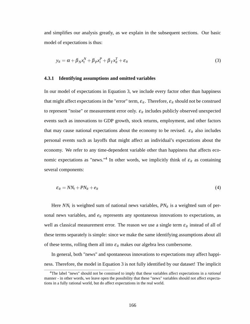
and simplifies our analysis greatly, as we explain in the subsequent sections. Our basic

model of expectations is thus:

yit = α+β NxNt +β PxP

i +β T xTit + ε it (3)

4.3.1 Identifying assumptions and omitted variables

In our model of expectations in Equation 3, we include every factor other than happiness

that might affect expectations in the "error" term, ε it . Therefore, ε it should not be construed

to represent "noise" or measurement error only. ε it includes publicly observed unexpected

events such as innovations to GDP growth, stock returns, employment, and other factors

that may cause national expectations about the economy to be revised. ε it also includes

personal events such as layoffs that might affect an individual’s expectations about the

economy. We refer to any time-dependent variable other than happiness that affects eco-

nomic expectations as "news."4 In other words, we implicitly think of ε it as containing

several components:

ε it = NNt+PNit+ eit (4)

Here NNt is weighted sum of national news variables, PNit is a weighted sum of per-

sonal news variables, and eit represents any spontaneous innovations to expectations, as

well as classical measurement error. The reason we use a single term ε it instead of all of

these terms separately is simple: since we make the same identifying assumptions about all

of these terms, rolling them all into ε it makes our algebra less cumbersome.

In general, both "news" and spontaneous innovations to expectations may affect happi-

ness. Therefore, the model in Equation 3 is not fully identified by our dataset! The implicit

4The label "news" should not be construed to imply that these variables affect expectations in a rational

manner - in other words, we leave open the possibility that these "news" variables should not affect expecta-

tions in a fully rational world, but do affect expectations in the real world.

166

components of ε it include all correlated omitted variables. In other words:

Cov(ε it ,xNt ) 6= 0 (5)

Cov(ε it ,xTit ) 6= 0 (6)

Without any further assumptions, this would make it impossible for us to learn anything

interesting about the β coefficients in Equation 3 using our dataset. This is not surprising;

all regressions are subject to the possibility of correlated omitted variables, and even when

they include many covariates, must rely on assumptions in order to be identified. Fortu-

nately, we have two additional assumptions that allow us to learn some interesting things

about our β ’s. The first of these is the assumption that any piece of news that makes a per-

son more optimistic, or any positive spontaneous innovation in the person’s expectations,

also makes that person happier contemporaneously. In other words:

Cov(ε it ,xNt ) ≥ 0 (7)

Cov(ε it ,xTit ) ≥ 0 (8)

As we will see, this assumption allows us to set upper bounds on the effect of national

happiness and of transitory personal happiness on expectations.

Our second assumption is that neither news nor spontaneous innovations to expecta-

tions affects persistent personal happiness xPi . This assumption is motivated by the idea of

hedonic adaptation. Persistent personal happiness is assumed to be a fixed psychological

trait. Furthermore, we assume that hedonic adaptation happens within six months.

Finally, note that we have not included an individual fixed effect in our model of expec-

tations. We will discuss this in a later section.

167

4.3.2 Effect of national happiness

In the aggregate analysis, we examined the effect of national happiness on national expecta-

tions. In this section we look at the effect of national happiness on individual expectations.

In other words, in this section we ask: “If a person wakes up on a certain day and finds that

the nation as a whole is much happier than normal, is she likely to be much more optimistic

about the economy than she normally is?”

The national happiness component xNt is assumed to be the same for all individuals. The

average happiness of a number of individuals interviewed on the same day can, roughly

speaking, be thought of as a noisy proxy for xNt . For our estimation of β N , we find it useful

to define a quantity x−it that we call the "daily other-mean" of happiness - in other words,

the average happiness of all individuals other than individual i who are interviewed on the

same day as individual i:

x−it ≡1

mt−1∑j 6=i

x jt (9)

Here mt is the number of people contacted on day t. Since we assume that only national

happiness (and not either of the two kinds of personal happiness) is correlated across indi-

viduals, x−it is a proxy for xNt . We will also find it useful to define "de-national-meaned"

happiness, xit :

xit ≡ xit− x−it (10)

We estimate β N by the method of moments. Consistent estimation of β N is not possible,

given the endogeneity discussed in Section 4.3.1. However, we use moment conditions to

define an asymptotically biased estimate β N . β N is a consistent estimate of β N+bias:

β N

P−→ β N+Cov(ε it ,x

Nt )

Var(xNt )

(11)

168

See Appendix III.A.2.1 for the derivation of β N . Mechanically, the moment condition

that identifies β N is equivalent to the parameter estimate from an instrumental variables

regression of expectations yit on happiness xit , instrumenting for xit with x−it .

As stated above, we assume that the bias is positive; that is, that Cov(ε it ,xNt )≥ 0. β N is

therefore an upper bound on the true β N . We refer to β N as "the estimate of β N ," keeping

in mind that it is really an estimate of an upper bound of β N and that the estimate standard

errors for β N are actually the standard errors of an upper bound on β N . We use this sloppy

terminology throughout the remainder of the paper, though we periodically remind the

reader when an estimate is upwardly biased.

The estimates of β N for our various expectation variables are in Table III.8. The es-

timate is not statistically significant for any of these variables except for bus12 (p-value

of 0.032). For bus12, the point estimate is 0.632, which is a substantial effect. As in the

aggregate analysis, there appears to be a correlation between national happiness and bus12.

However, the direction of causation is not identifiable.

We also care about the explanatory power of national happiness. Even if swings in the

national mood can cause swings in expectations, these swings may be only a tiny fraction

of the total. We can estimate an upper bound on the fraction of the variance of yit that can

be explained by xNt (see Appendix III.A.3). We call this value R2

N . We estimate R2N to be

0.004 for bus12, and lower for other expectation variables - a tiny amount, even though it

is an upper bound. The reason for this is that the national mood simply does not swing by

very much; see Table III.7 for estimates of the variances the three happiness component.5

The variance of xNt is two orders of magnitude lower than the variance of either of the other

two components.

Individual-level analysis essentially confirms the conclusions of the aggregate analysis.

Bus12 and national happiness are related, but the direction of causality is unknown and may

be due any one of a large number of omitted variables. National happiness is not detectably

5These are in terms of number of unconditional standard deviations of total happiness.

169

related to any other expectation variable. Also, the power of national happiness to explain

variations in expectations is negligible. Therefore, we find very little evidence to support

the "affective animal spirits" hypothesis at the national level, though the correlation with

bus12 is interesting and worthy of further study.

4.3.3 Effect of transitory personal happiness

In this section we look at the effect of transitory happiness fluctuations on individual ex-

pectations. In other words, we ask: “If a person wakes up on a certain day and finds that

she is much happier, relative to other people, than normal, is she likely to be much more

optimistic about the economy than she normally is?”

To answer this question, we estimate an upper bound on β T . Again, we use the method

of moments to find an estimate of the upper bound on β T , which we call β T . Mechan-

ically, β T is the same as the parameter estimate from an IV regression of the change in

happiness between an individual’s first and second contacts, ∆yit , on the change in de-

national-meaned happiness, ∆xit . See Appendix III.A.2.2 for a derivation of the moment

conditions. Essentially, we are just performing an instrumental variable regression in first

differences, after differencing out national happiness.

This estimate is another upper bound, this time an upper bound on the true effect of

swings in personal happiness on swings in expectations. The bias exists for the same reason

as in the last section; swings in happiness and optimism may cause each other. Again, we

sloppily refer to this estimate as the "estimate of β T ."

Estimates of β T for our various expectation variables are in Table III.9. A large fraction

of these are significant at the 5% level. Most of the point estimates are on the order of 0.05;

this is about an order of magnitude smaller than the correlation between expectations and

happiness found at the beginning of this section. Most of the fact that happier people are

more optimistic is explained by the individual fixed effect.

As in the previous section, we calculate an upper bound on the fraction of the variance

170

of yit that can be explained by xTit . These values are never more than 0.001; we estimate that

no more than 0.1% of swings in an individual’s expectations can be explained by swings in

her own happiness. In reality, given the influence of personal news - layoffs and the like -

on both expectations and happiness, it is likely that the true causal effect of happiness on

expectations is considerably smaller. How small, or whether the effect exists at all, is a

question beyond the scope of this analysis; we attempt to be as favorable as possible to the

hypothesis that swings in happiness cause swings in expectations, and to show that even in

the most favorable case, the effect is not substantial.

4.3.4 Effect of persistent personal happiness

If swings in happiness do not account for the correlation between happiness and expec-

tations, then most of the relationship must be due to the individual fixed effect, or what

psychologists call the "trait" of happiness. Here we confirm that intuition. We use the

method of moments to derive a moment ratio that is equivalent in population to β P (see

Appendix III.A.2.3). This moment ratio is mechanically equivalent to the parameter esti-

mate from an IV regression of expectations on happiness, instrumenting for an individual’s

happiness with the same individual’s happiness at the other contact date, after instrument-

ing for happiness at the second contact date with de-national-meaned happiness at the first

contact date. (See Appendix III.A.2.3). In other words, if xi2 is an individual’s happiness

at the second contact date, we perform an IV regression of yi2 on xi2, instrumenting for xi2

with xi1, to obtain an estimate of β P. We assume that there is no individual fixed effect in

expectations apart from the effect of persistent personal happiness; hence, unlike in pre-

vious estimators, we consider our estimates of β P to be consistent.6 Our estimates are in

Table III.9. We see that, as predicted, our estimates of β P are about an order of magnitude

larger than our estimates of β T , and are very similar to the overall correlation between

happiness and expectations.

6This is motivated by the voluminous literature on hedonic adaptation.

171

As a robustness check, we can allow for persistent personal happiness to be correlated

with slow-moving spontaneous innovations to expectations at the national level - in other

words, we can relax the assumption of hedonic adaptation with respect to national news.7

The model in Equation 3 will then become:

yit = α+ γ t+β NxNt +β PxP

i +β T xTit + ε it (12)

To see if this changes the analysis, we simply demean yit at the daily level - i.e., we de-

fine yit equivalently to xit above - and repeat the above estimation using yit as our dependent

variable. The results are virtually unchanged (results not shown).

4.3.5 Fixed effects in expectations

In our previous analysis, we assumed that there is no individual fixed effect in expectations

other than the fixed effect attributable to persistent personal happiness. This may not be

the case; for example, rich people may be permanently more optimistic than poor people.

On one hand, any sort of individual fixed effect in expectations is interesting, since it raises

the possibility of composition bias in expectations. However, if individual fixed effects

in expectations are caused by differences in psychological traits such as happiness, that is

particularly interesting. Thus, we repeat the analysis in Section 4.3.4, but we add covariates

representing several slow-changing variables:

• age

• education level

• income

• a dummy for homeownership

7This would happen if, for example, shocks to national economic variables such as GDP growth were

serially correlated at the 6-month horizon, but if people were not aware of this correlation, leading them to

be repeatedly "surprised" by the realizations of these variables.

172

• wealth invested in stocks

• a dummy for white non-Hispanic race

The estimates of β P with these covariates are included are shown in Table III.9. The

estimates are only slightly changed from the estimates without covariates. Although there

may be other omitted variables that account for the effect, it is clear that the effect of per-

sistent personal happiness on expectations is very hard to explain with non-psychological

variables.

4.3.6 Model with survey response error

Until now, we have worked with the happiness index xit , instead of the individual answers

to the four questions on our questionnaire. However, exploiting the variation between the

answers to those four questions may help us get better estimates of β P and β T . We do that

in this section.

Also, in this section we want to deal explicitly with the fact that our questions do not

actually measure true happiness. It is possible that survey respondents differ more in how

they respond to questions than in how they actually feel. So in this section we include

"response errors" in our model of happiness. We consider response errors of four basic

types:

• Errors that depend only on the individual (individual fixed effects)

• Errors that depend on individual and the time of the survey

• Errors that depend on the individual and the wording of the question, but are fixed in

time

• Errors that depend on the individual, the wording of the question, and the time of the

survey

173

We represent these four response errors as si, uit , viq, and witq, respectively. For simplic-

ity’s sake we assume that all of these response errors show up in the happiness questions,

though mathematically it doesn’t matter if response errors in the expectation questions exist

as well. So our new model of happiness is:

xitq = xNt + xP

i + xTit + si+uit+ viq+witq (13)

This assumes that all four questions are noisy measures of the same thing (affect va-

lence, happiness, etc.).

Our new model of expectations is:


i +β T xTit +β ssi+β uuit+β vviq+β wwitq+ ε it (14)

Derivations of the estimates for this model are in Appendix III.A.4. The estimate for

β N is unchanged. Two things about the estimates of β P and β T are different. First of all,

they are no longer estimates of β P and β T ! They are now estimates of (1− θ)β P+ θβ S

and (1−ξ )β T +ξ β T , where θ and ξ are parameters (both between 0 and 1) representing

the relative importance of the individual-specific response errors si and uit :

θ =Var(si)

Var(si)+Var(xPi )

(15)

ξ =Var(uit)

Var(uit)+Var(xTit )

(16)

In other words, if you believe that most of the variance in survey responses is due to

response error, then the estimates in this paper do not mean much; however, if you believe

that true values vary about as much as response error, then the results in this paper stand.

The second change from the previous sections is that our estimates, and the associated

R2 values (again, upper bounds on the true values), are now both multiplied by correc-

174

tion factors that come from the variance across the four affect questions (see Appendix

III.A.4.6). The correction factors are 1.38 for persistent personal happiness and 0.536 for

transitory personal happiness. Results for the new estimates for β P and β T , and the asso-

ciated R2 values, can be seen in Table III.11. After accounting for cross-question response

errors, the estimates of the effect of persistent personal happiness grow substantially while

the estimates of the effect of transitory personal happiness shrink substantially. This con-

firms our basic story.

4.3.7 Other Emotions

Our survey only contains questions about two kinds of emotion: happiness and sadness.

But if we are really going to test the "affective animal spirits" hypothesis, shouldn’t we

look at other emotions too? What about fear, or excitement, or anger?

Our answer to this question is that different emotional states are probably correlated

with each other. A person who answers that she is “happy” is probably more likely to

report that she is "excited," and a person who answers that she is "sad" is probably more

likely to answer that she is "worried" or "afraid." If different emotions are very correlated,

our results hold true for all emotions; only an affect measure that was nearly orthogonal to

happiness would still be a candidate for affective animal spirits. Our result is thus much

broader than the limited scope of our survey questions might suggest.

To demonstrate this, we do a simple numerical experiment. Suppose that self-reported

happiness is equal to true happiness , and that there exists another emotion – call it “Emo-

tion Z” – that is imperfectly correlated with happiness. For simplicity, assume that Emotion

Z has only a transitory component, zit . Then we can write:

xit = ρzit+ ς it (17)

175

Now assume that affective animal spirits are in fact caused by Emotion Z:

yit = α+β zzit+ ε it (18)

We can show that R2z , the percentage of the variance of expectations explained by

swings in Emotion Z, is bounded above by 1ρ

R2T . In order for swings in Emotion Z to

explain an economically significant amount of the swings in expectations, ρ must be very

very small. For example, if ρ is equal to 0.2, then swings in Emotion Z explain no more

than 0.02% of swings in expectations.

4.3.8 Subgroup Happiness

One final interesting possibility is that different demographic subgroups have common

emotions. Suppose that there is a national election in the U.S., which the Democrats win.

The happiness of Democrats surges; that of Republicans plummets by an equal amount.

Since the nation is evenly divided between Republicans and Democrats (suppose the hap-

piness of Independents is unchanged), the election will register no change in "national

happiness" as we have defined it up until now. But if Democrats and Republicans have dif-

ferent roles in the economy – for example, if Republicans are more likely to be investors – it

is possible to imagine that the emotional reaction to the election could have an effect on the

economy. The presence of group effects could introduce additional bias into our estimates

of β T and β P in the previous section. Fortunately, our data includes many demographic

characteristics that can be used to test this hypothesis.

We add two more components to the model of happiness – 1) a “persistent group hap-

piness” component that represents the long-term happiness of a particular group (e.g., if

Democrats are on average happier than Republicans), and 2) a “transitory group happi-

ness” component that represents differential changes in these groups that arise in response

to national events. Define γ i as a dummy that indicates membership in some group (-1 or

176

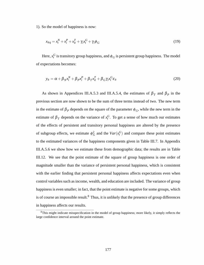
1). So the model of happiness is now:

xitq = xNt + xP

i + xTit + γ ix

Gt + γ iφG (19)

Here, xGt is transitory group happiness, and φG is persistent group happiness. The model

of expectations becomes:


i +β T xTit +β Gγ ix

Gt ε it (20)

As shown in Appendices III.A.5.3 and III.A.5.4, the estimates of β T and β P in the

previous section are now shown to be the sum of three terms instead of two. The new term

in the estimate of β P depends on the square of the parameter φG, while the new term in the

estimate of β T depends on the variance of xGt . To get a sense of how much our estimates

of the effects of persistent and transitory personal happiness are altered by the presence

of subgroup effects, we estimate φ2G and the Var(xG

t ) and compare these point estimates

to the estimated variances of the happiness components given in Table III.7. In Appendix

III.A.5.6 we show how we estimate these from demographic data; the results are in Table

III.12. We see that the point estimate of the square of group happiness is one order of

magnitude smaller than the variance of persistent personal happiness, which is consistent

with the earlier finding that persistent personal happiness affects expectations even when

control variables such as income, wealth, and education are included. The variance of group

happiness is even smaller; in fact, that the point estimate is negative for some groups, which

is of course an impossible result.8 Thus, it is unlikely that the presence of group differences

in happiness affects our results.

8This might indicate misspecification in the model of group happiness; more likely, it simply reflects the

large confidence interval around the point estimate.

177

5 Discussion

Our results are bad news for the "affective animal spirits" hypothesis of business cycles.

The upper bounds on the explanatory power of national and transitory personal happiness

mean that emotion is not a major cause of "animal spirits"; even swings in the happiness

of a key individual or small group of individuals are unlikely to move those individuals’

expectations by much. And the effect on real economic variables - at least, if it acts through

expectations - must be even smaller. For example, let’s take the most optimistic estimate

of the effect of swings in consumer confidence on GNP - 26%, the highest value reported

by Matsusaka and Sbordone (1995). Using our estimates for R2T , we can conclude that no

more than 0.026% of swings in GNP can possibly be explained by swings in happiness.

Suppose that it is actually fear that drives business cycles, and set the covariance between

fear and happiness equal to only -0.2. Then less than 0.005% of the swings in GNP are

due to fear. Remember, also, that these are upper bounds on upper bounds; the true value

is bound to be much lower.

However, our results may be interesting for the field of finance. In finance, a profitable

trading opportunity does not have to have a large R-squared; it just has to exist. Some pa-

pers have found that consumer confidence predicts stock returns, but consumer confidence

surveys are very infrequent. Happiness surveys, however, are easy to do. Our results show

a correlation between happiness (national or personal) and one measure of expectations

(bus12). If this component of consumer confidence predicts stock returns, then traders may

gain useful information from measuring national happiness, or from paying attention to

public data on happiness as it emerges.

The hypothesis of "affective animal spirits" is often put forth as an alternative to Ratio-

nal Expectations. Barsky and Sims (2008) showed, in the context of a specific macroeco-

nomic model, that autonomous movements in consumer confidence don’t cause swings in

real economic variables. The results in this paper yield a similar result. Does this mean that

our results support Rational Expectations? Actually, no. Rational Expectations requires ex-

178

pectations to be unbiased estimates of the predictions of the best model of the economy.

But if expectations depend on psychological traits, this cannot be the case. Suppose that

half of the population is naturally optimistic all the time, and half is naturally pessimistic,

regardless of economic conditions. A composition shock - say, if the pessimistic people

all decided to take the day off - would cause a bias to appear in the expectations of the

representative agent.

In Section 4.3.3, we found that persistent personal happiness has a statistically signifi-

cant effect on most survey measures of economic expectations. Persistent personal happi-

ness is a psychological trait. This means that if A) survey responses are a good measure

of expectations, and if B) survey responses are a good measure of true happiness, then

this finding indicates the presence of composition effects in expectations. Strict versions

of Rational Expectations theory hold that composition effects in expectations can’t exist,

because aggregate expectations would then be vulnerable to a composition shock (for ex-

ample, if a bunch of happy people suddenly moved to Zambia). Because the economy does

not usually suffer large composition shocks, the anomaly is unlikely to make a big differ-

ence in economic outcomes. But it may signal the existence of a wider class of ways in

which individual psychological traits cause departures from rationality.

Our results are of minor importance for the cognitive economics literature. Studies have

shown that recessions make people less happy. Our negative results for national and transi-

tory personal happiness show that this effect probably does not work through expectations.

In other words, recessions are not making people unhappy because they are making them

pessimistic. This means that recessions’ adverse effect on happiness probably cannot be

allayed by taking steps to raise expectations about the economy’s long-term performance.

179

6 Conclusion

In this paper, we investigated the relationship between affect and economic expectations, as

measured by surveys. We found mostly no correlation between average national happiness

and either average expectations or individual expectations, with one possible exception (the

variable bus12), which deserves further study. In fact, we found only small and short-lived

movements in average national happiness, meaning that the "national mood" is unlikely

to drive much of anything. At the individual level, we found that the causal effect of

happiness swings on expectation swings, at the 6-month frequency, is much smaller than

the cross-sectional correlation; generally happy people are generally more optimistic, but

this is a long-term fixed effect. We also found that fluctuations in happiness explain only a

tiny percent of the observed fluctuations in expectations. This result is robust to question-

specific response errors. It is also reasonably robust to misspecification of the relevant

affective state; our results imply that fear, excitement, and other emotions are also unlikely

to be significant causes of business cycles. However, we did find that individual fixed

effects in happiness are associated with more optimistic expectations

The negative results in this paper deal a blow to the popular notion of “animal spirits” as

being an emotional phenomenon. Even if business cycles can be caused by changes in the

public’s expectations, those expectation changes are almost certainly not caused by changes

in the national mood, or in the mood of any special subset of the population. Although one

might search for other emotions to explain expectation movements, such emotions would

have to be unrelated to happiness; thus, we believe that it will be much more useful for

advocates of “animal spirits” theories of the business cycle to look at expectation-formation

processes rather than emotional factors. On the other hand, our results raise the possibility

that survey measures of affect might be an important piece of data for financial traders.

Also, the importance of slowly-changing psychological traits on expectations would be

troubling for certain theories of individual rationality; further study, to confirm this effect

and to establish the causality between fixed effects in expectations and fixed effects in

180

happiness, is warranted.

Future research in this area should also focus on using a more diverse set of measures of

both affect and expectations. Alternate measures of expectations might include betting on

futures markets. Alternate measures of emotion might include questions on a wider range

of emotions, or even neurological studies using fMRI to track emotional states.

181

182

Tables and Figures

Figure III.1: Bus12 and Happiness (Monthly Aggregates)

-0.6

-0.4

-0.2

0

0.2

0.4

0.6

0.8

1 7 13 19 25 31 37 43 49 55 61 67

Stan

dar

d D

evia

tio

ns

Month

Bus12 Happiness

183

Table III.1a: Text of Consumer Confidence Questions

pago “Would you say that you (and your family living there) are better off or

worse off financially than a year ago?”

pexp “Do you think that a year from now you (and your family living there) will

be better off financially, or worse off, or just about the same as now?”

bus12 “Do you think that during the next 12 months we’ll have good times

financially, or bad times, or what?”

bus5

“Which would you say is more likely – that in the country as a whole we’ll

have continuous good times during the next 5 years or so, or that we will

have periods of widespread unemployment and depression, or what?”

dur “Generally speaking, do you think now is a good time or a bad time for

people to buy major household items?”

184

Table III.1b: Text of Other Expectations Questions

v228

“Compared with 5 years ago, do you think the chances that you (and your

husband/wife) will have a comfortable retirement have gone up, gone

down, or remained about the same?”

hom “Generally speaking, do you think now is a good time or a bad time to buy

a house?”

car “Do you think the next 12 months will be a good time or a bad time to buy

a vehicle?”

homeval

“Do you think the present value of your home – I mean what it would

bring you if you sold it today – has increased compared with a year ago,

decreased, or stayed about the same?”

bago “Would you say that at the present time business conditions are better or

worse than they were a year ago?”

bexp

“A year from now, do you expect that in the country as a whole business

conditions will be better, or worse than they are at present, or just about

the same?”

govt

“As to the economic policy of the government – I mean steps taken to

fight inflation or unemployment – would you say the government is doing

a good job, only fair, or a poor job?”

unemp

“How about people out of work during the coming 12 months – do you

think that there will be more unemployment than now, about the same, or

less?”

185

Table III.1c: Text of Happiness Questions

h1 "Much of the time during the past week, you were happy. Would you say yes or

no?"

h2 "Much of the time during the past week, you felt depressed. Would you say yes or

no?"

h3 "Much of the time during the past week, you enjoyed life. Would you say yes or

no?"

h4 "Much of the time during the past week, you felt sad. Would you say yes or no?"

186

Table III.2: Descriptive Statistics

Variable Mean (0-100) Std. Dev. Monthly Autocorrelation

Pago 45.37 42.18 0.90

pexp 56.49 36.83 0.65

bus12 36.83 46.57 0.81

bus5 42.19 43.82 0.69

dur 68.79 45.64 0.86

v228 39.38 35.63 0.93

hom 71.10 45.05 0.86

car 64.70 47.30 0.68

homeval 48.74 40.50 0.96

bago 31.31 44.08 0.92

bexp 50.28 35.30 0.87

govt 39.34 34.89 0.83

unemp 65.10 33.67 0.94

happiness -0.09

187

Table III.3: Happiness Question Correlations

h1 h2 h3 h4

h1 1

h2 0.583 1

h3 0.572 0.464 1

h4 0.526 0.609 0.417 1

Table III.4: Autocorrelations of Aggregate Variables

Lag (months) Autocorrelation of Happiness Autocorrelation of Bus12

1 -0.09 0.81

2 0.09 0.64

3 0.03 0.58

4 -0.13 0.53

5 0.14 0.50

188

Table III.5: VAR of Bus12 and Happiness

RHS Variable

LHS Variable Lag (months) Bus12 Happiness

Bus12

1 0.912*** 0.161**

2 -0.114 -0.368***

3 0.149 0.326***

4 0.045 -0.177*

5 -0.095 0.0784

Happiness

1 0.016 0.199

2 -0.177 0.050

3 -0.092 0.119

4 -0.552** -0.140

5 0.279 0.044

Note: *** = significant at the 1% level; ** = significant at the 5% level; * = significant at

the 10% level

189

Table III.6: OLS of Expectations on Happiness

LHS Variable Effect of Happiness Std. Error

pago 0.163 0.006

pexp 0.066 0.007

bus12 0.110 0.007

bus5 0.137 0.007

dur 0.083 0.007

v228 0.119 0.006

hom 0.086 0.006

car 0.085 0.007

homeval 0.039 0.007

bago 0.081 0.007

bexp 0.081 0.007

govt 0.101 0.007

unemp 0.072 0.008

Note: all coefficients listed are significant at the 1% level.

190

Table III.7: Estimated Variances of Happiness Components

Component Estimated Variance

National Happiness 0.006

Transitory Personal Happiness 0.431

Persistent Personal Happiness 0.561

Note: Total happiness is normalized to have a variance of 1.

Table III.8: Effect of National Happiness

LHS Variable Effect of National Happiness Std. Error R2

N

pago -0.254 0.286 0.000

pexp 0.112 0.272 0.000

bus12 0.505* 0.263 0.002

bus5 0.268 0.260 0.000

dur 0.252 0.288 0.000

v228 0.242 0.267 0.000

hom -0.108 0.288 0.000

car -0.464 0.317 0.001

homeval 0.277 0.259 0.000

bago 0.538* 0.304 0.002

bexp 0.432 0.296 0.001

govt -0.114 0.283 0.001

unemp 0.495 0.288 0.000


the 10% level

191

Table III.9: Effects of Personal Happiness Components

LHS Variable Transitory Effect Persistent Effect

Persistent Effect

(Covariates Included) R2

T

pago .054***

(.009)

.273***

(.021)

.316***

(.040) 0.001

pexp .027***

(.010)

.099***

(.021)

.317***

(.038) 0.000

bus12 .052***

(.010)

.153***

(.022)

.318***

(.043) 0.001

bus5 .022**

(.010)

.270***

(.022)

.319***

(.041) 0.000

dur .025***

(.011)

.143***

(.022)

.320***

(.040) 0.000

v228 .052***

(.009)

.213***

(.021)

.321***

(.042) 0.001

hom .007

(.010)

.185***

(.021)

.322***

(.036) 0.000

car .013

(.010)

.165***

(.022)

.323***

(.039) 0.000

homeval .007

(.009)

.061***

(.026)

.324***

(.043) 0.000

bago .036

(.010)

.091***

(.022)

.325***

(.042) 0.001

bexp 030***

(.010)

.113***

(.021)

.326***

(.040) 0.000

govt .035***

.188***

(.022)

.327***

(.041) 0.000

unemp .045***

(.010)

.095***

(.021)

.328***

(.040) 0.001


the 10% level

192

Table III.10a: Covariance Matrix for Transitory Correction

Factor

2.223 1.006 0.697 0.981

0.999 2.136 0.516 1.125

0.698 0.523 1.230 0.501

0.983 1.130 0.499 2.720

Correction Factor = 0.536

Table III.10b: Covariance Matric For Persistent Correction

Factor

0.553 0.449 0.373 0.432

0.463 0.560 0.319 0.515

0.356 0.303 0.323 0.288

0.485 0.534 0.340 0.608

Correction Factor = 1.38

193

Table III.11: Personal Happiness (With Response Errors)

LHS Variable Transitory Effect Persistent Effect R2

T

pago 0.029 0.376 0.000

pexp 0.015 0.136 0.000

bus12 0.028 0.212 0.000

bus5 0.012 0.373 0.000

Dur 0.013 0.197 0.000

v228 0.028 0.294 0.000

Hom 0.004 0.255 0.000

Car 0.007 0.228 0.000

Homeval 0.004 0.084 0.000

Bago 0.019 0.125 0.000

bexp 0.016 0.156 0.000

govt 0.019 0.260 0.000

unemp 0.024 0.132 0.000

Note: Standard errors are the same as in Table 8.

194

Table III.12: Group Effects

Group

Square of persistent group

happiness

Variance of transitory group

happiness

Political 0.005 0.005

Over 44 0.000 -0.002

Income over $100k 0.013 -0.013

Homeowner 0.015 -0.017

Stockholder 0.025 -0.024

College Degree 0.011 -0.014

Race (White/Nonwhite) 0.003 0.000

195

Appendix III.A: Models and Derivations

A.1. Definitions

R-squared values:

2 2 ( )N

N N tR Var x

2 2 ( )

( )

T

itT T

it

Var xR

Var y

2 2 ( )P

P P iR Var x

Note that 2itx represents individual i ’s (self-reported) happiness on the date of her

second interview, and itx represents an individual’s change in happiness between her

first and second interview, etc.

A.2. Basic Model

A.2.1. Effect of N

tx

An instrumental variables regression of ity on itx , using itx as an instrument for itx ,

yields the following estimator:

( , )

( , )

it itN

it it

Cov y x

Cov x x

Expanding the numerator and denominator, we get:

196

( , ) ( , )N P T N P T

it it N t P i T it it t i itCov y x Cov x x x x x x

( , ) ( , )N P T N P T

it it t i it t i itCov x x Cov x x x x x x

To simplify these expressions, we use the assumptions:

( , ) ( , ) 0P T

it j it jtCov x Cov x

( , ) ( , ) ( , ) 0N P T P N T

it i it i it iCov x x Cov x x Cov x x

( , ) ( , ) 0P P T T

i j it jtCov x x Cov x x where j i

This leaves us with simplified expressions for numerator and denominator:

( , ) ( ) ( , )N N

it it N t it tCov y x Var x Cov x

( , ) ( )N

it it tCov x x Var x

Dividing these expressions and simplifying, we get:

( , ) ( , )

( , ) ( )

N

it it it tN N

it it t

Cov y x Cov x

Cov x x Var x

We have assumed that the second term is positive. Thus, N is an estimate of an upper

bound on N .

A.2.2. Effect of T

itx

197

An instrumental variables regression of ity on itx , using itx as an instrument for itx ,


( , )

( , )

ititT

it it

Cov y x

Cov x x


2 1 2 1 2 1 2 1 2 1

2 1 2 1 2 1

( ,[ ] [ ]) ( [ ] [ ]

[ ],[ ] [ ])

N N T T

it it it it it it N t t T it it

T T T T

it it it it it it

Cov y y x x x x Cov x x x x

x x x x

2 1 2 1 2 1

2 1 2 1 2 1 2 1

( , [ ] [ ])

([ ] [ ],[ ] [ ])

it it it it it it

N N T T T T T T

t t it it it it it it

Cov x x x x x x

Cov x x x x x x x x

To simplify these expressions, we use the following additional assumptions:

1 2 2 1

2 2 1 2 2 1 1 1

( , ) ( , ) 0

( , ) ( , ) ( , ) ( , ) 0

T T

it it it it

T T T T

it jt it jt it jt it jt

Cov x Cov x

Cov x Cov x Cov x Cov x

This leaves us with simplified expressions for the numerator and denominator:

2 1 2 1 2 1( ,[ ] [ ]) 2 ( ) ( , )T T

it it it it it it T it it itCov y y x x x x Var x Cov x

2 1 2 1 2 1( , [ ] [ ]) 2 ( )T

it it it it it it itCov x x x x x x Var x

Dividing these expressions, we get:

198

( , ) ( , )

( , ) ( , )

it itit itT

it itit it

Cov y x Cov x

Cov x x Cov x x

Again, we have assumed that the second term is positive. Thus, T is an estimate of an

upper bound on T .

A.2.3. Effect of P

ix

An instrumental variables regression of 2ity on

2itx , using 1itx as an instrument for

2itx ,


12

12

( , )

( , )

itit

P

it it

Cov y x

Cov x x


2 1 1 2 2 2 1 1 1( , ) ( , )N P T P P T T

it it it N t P i T it it i it it itCov y x x Cov x x x x x x x

2 1 1 2 2 1 1 1( , ) ( , )N P T P P T T

it it it t i it i it it itCov x x x Cov x x x x x x x

To simplify these expressions, we use assumptions already listed above. This leaves us

with simplified expressions for numerator and denominator:

2 1 1( , ) ( )P

it it it P iCov y x x Var x

2 1 1( , ) ( )P

it it it iCov x x x Var x

Dividing these expressions, we get:

199

12

12

( , )

( , )

itit

P

it it

Cov y x

Cov x x

Thus given our assumptions, P is an unbiased estimator of P .

A.3. Variances of Happiness Components

Our model of observed happiness, given in Equation 2, is:

N P T

it t i itx x x x

As shown in the previous section the variances of the happiness components can be

computed thus:

( ) ( , )N

t it itVar x Cov x x

2 1 1( ) ( , )P

i it it itVar x Cov x x x

1( ) ( , )

2

T

it it it itVar x Cov x x x

The estimated variances of the three happiness components are listed in Table 8.

A.4. Model with response errors

A.4.1. Happiness with response errors

Our model of happiness with response errors, given in Equation 12, is:

200

N P T

itq t i it i it iq itqx x x x s u v w

N

tx , P

ix , T

itx , is , itu , iqv , and itqw are taken to be iid mean-zero random variables that are

orthogonal to one another.

In our data set, self-reported happiness is just the average of these four components. We

write:

N P T

it t i it i it i itx x x x s u v w

Where:

1 2 3 4

1 2 3 4

1 2 3 4

( ) / 4

( ) / 4

( ) / 4

it it it it it

i i i i i

it it it it it

x x x x x

v v v v v

w w w w w

Our expressions for the variances of the happiness components now represent the sum of

the variances of the happiness components and (where applicable) of the response errors

that are not observably different from the happiness components:

( , ) ( )N


2 1 1( , ) ( ) ( )P

it it it i iCov x x x Var x Var s

1( , ) ( ) ( )

2

T

it it it it itCov x x x Var x Var u

201

A.4.2. Expectations with response errors

We may safely assume that expectation questions produce similar “response errors”.

Allowing that expectation-question response errors may be correlated with happiness-

question response errors, our model of expectations becomes:

N P T

it N t P i T it s i u it ity x x x s u

This model includes the effect of a respondent’s mood on their expectations ( P for the

long-term components of mood, T for the transitory components); the relationship

between a respondent’s tendency to answer happiness-related questions in a particular

way and his/her tendency to answer expectation-related questions in a particular way ( s

and u ); and the potential for the social construction of expectations ( N )1. Again, we

assume that the error term, it , is mean-zero and is uncorrelated with P

ix , is , and itu .

Our purpose is, again, to identify the coefficients N , P , and T . For the latter two,

this will no longer be possible; we will only be able to identify expressions that contain

the effects of the response styles, s and u . Obtaining economically significant results

must depend on our belief that the variances of is and itu are small.

A.4.3. Effect of N

tx with response errors

We now define the “daily other mean” of happiness, itx , as:

1 The question-specific response style terms from the measurement model - iqv and itqw - do not

enter the structural model, since a respondent’s answer to an expectation-related question is presumably not related to the particular set of happiness-related questions that were asked on his/her survey – especially because the latter are asked after the former.

202

N P T

it t it it it it it itx x x x s u v w

Using the same regression as in the basic model, our estimator is:

( , )

( , )

it itN

it it

Cov y x

Cov x x

We can rewrite the numerator and denominator:

( , ) ( ,

)

N P T

it it N t P i T it s i u it it

N P T

t i it i it i it

Cov y x Cov x x x s u

x x x s u v w

( , ) ( ,

)

N P T

it it t i it i it i it

N P T

t i it i it i it

Cov x x Cov x x x s u v w

x x x s u v w

We can simplify these expressions using the orthogonality assumptions:

203

( , ) ( , ) ( , )

( , ) ( , ) ( , ) 0

( , ) ( , ) ( , ) ( , ) 0

( , ) ( , ) ( , ) ( , ) 0

( , ) (

P T

it j it jt it j

it jt it j it jt

N N N N

t j t jt t j t jt

P P P P

i j i jt i j i jt

T

it j it

Cov x Cov x Cov s

Cov u Cov v Cov w

Cov x s Cov x u Cov x v Cov x w


Cov x s Cov x

, ) ( , ) ( , ) 0

( , ) ( , ) ( , ) ( , )

( , ) ( , ) 0

( , ) ( , ) ( , ) 0

T T T

jt it j it jt

i it i i i it it j

it jt i jt

i j i j it jt

u Cov x v Cov x w

Cov s u Cov s v Cov s w Cov u v

Cov u w Cov v w

Cov s s Cov v v Cov w w

These let us cancel most of the terms in the numerator and denominator, leaving us with:

( , ) ( ) ( , )N N


( , ) ( )N


Dividing then yields:

( , ) ( , )

( , ) ( )

N

it it it tN N

it it t

Cov y x Cov x

Cov x x Var x

Thus, the presence of response errors does not change our result for the effect of N

tx .

A.4.4. Effect of T

itx with response errors

This time, our estimator is:

204

( , )

( , )

ititT

itr itq

Cov y x

Cov x x

Expanding the numerator and denominator, we have:

2 1 2 1 2 1 2 1 2 2

2 1 2 1

2 1 2 1 2 1

2 1 2 1 2 1

( ,[ ] [ ]) ( [ ] [ ]

[ ] [ ],

[ ] [ ] [ ]

[ ] [ ] [ ])

N N T T

it it it it it it N t t T it it

u it it it it

T T

it it it it it it

T T

it it it it it it

Cov y y x x x x Cov x x x x

u u

x x u u w w

x x u u w w

2 1 2 1 2 1 2 1 2

2 1 2 1

2 1 2 1 2 1

2 1 2 1 2 1

1( , [ ] [ ]) ([ ] [ ]

[ ] [ ],

[ ] [ ] [ ]

[ ] [ ] [ ])

N N T T

it q it q it r it r it r it r t t it i

it it it q it q

T T

it it it it it r it r

T T

it it it it it r it r

Cov x x x x x x Cov x x x x

u u w w

x x u u w w

x x u u w w

We can simplify these with the aforementioned assumptions, plus the following:

1 2 2 2

1 2 1 2

( , ) ( , ) 0

( , ) ( , ) 0

T T

i i i j

i i i i

Cov x Cov x

Cov u Cov w

Simplified, the numerator and denominator become:

2 1 2 1 2 1( ,[ ] [ ]) 2 ( ) ( ) ( , )T T

it it it it it it T it u it it itCov y y x x x x Var x Var u Cov x

2 1 2 1 2 1( , [ ] [ ]) 2 ( ) ( )T

it it it it it it it itCov x x x x x x Var x Var u

We take the ratio of the two, to get:

205

2 1 2 1 2 1

2 1 2 1 2 1

( , [ ] [ ]) ( , )(1 )

( , [ ] [ ]) ( ) ( )

T

i i i i i i it itT u T

i q i q i r i r i r i r it it

Cov y y x x x x Cov x

Cov x x x x x x Var x Var u

Where:

( )

[ ( ) ( )]

it

T

it it

Var u

Var x Var u

As before, if the variance of itu is small relative to the variance of T

itx , then

(1 ) T u is close to T .

We can decompose the moment ratio for (1 ) T u into the product of a moment

ratio and a “correction factor”:

2 1 2 1 2 1

2 1 2 1 2 1

2 1 2 1 2 1

2 1 2 1 2 1

( , [ ] [ ]) ( , )(1 )

( , [ ] [ ]) ( ) ( )

( , [ ] [ ])

( , [ ] [ ])

T

i i i i i i it itT u T

i q i q i r i r i r i r it it

i i i i i i

i q i q i r i r i r i r

Cov y y x x x x Cov x

Cov x x x x x x Var x Var u

Cov x x x x x x

Cov x x x x x x

2 1 2 1 2 1

2 1 2 1 2 1

( , [ ] [ ])

( , [ ] [ ])

( , )

( ) ( )

i i i i i i

i i i i i i

T

it it

T

it it

Cov y y x x x x

Cov x x x x x x

Cov x

Var x Var u

The “correction factor” 2 1 2 1 2 1

2 1 2 1 2 1

( , [ ] [ ])

( , [ ] [ ])

i i i i i i


Cov x x x x x x

Cov x x x x x x

must only be

estimated once for all expectation variables. The denominator can be found by averaging

the off-diagonal elements of a cross-question covariance matrix of

2 1 2 1 2 1( , [ ] [ ])i q i q i r i r i r i rCov x x x x x x for all pairs of q and r (shown in Table 11).

206

Our estimate for the “correction factor” for T in this simple model is 1.38, and our

estimates for (1 ) T u can be found in Table 12. A quick inspection of this table

reveals that most estimates of (1 ) T u are neither large nor significant, a fact

which will be important in showing that transitory movements in happiness have

relatively little effect on economic expectations.

A.4.5. Effect of P

ix with response errors

Our estimator is now:

12

12

( , )

( , )

itit

P

it rit q

Cov y x

Cov x x

Expanding the numerator and denominator, we have:

2 1 1 2 2

2 2

1 1 1 1 1

1 1 1 1

( , ) (

,

( )

( ))

N P T

it it it N t P i T it

s i u it it

P P T T

i it it it i it i it

it it it i

Cov y x x Cov x x x

s u

x x x x s u v w

s u v w

2 1 1 2 2

2 2

1 1 1

1 1

1 1

( , ) (

( ),

( )

( ))

N P T

it q it r it r t i it

i it iq it q

P P T T

i it it it

i it ir it r

i it ir it r

Cov x x x Cov x x x

s u v w

x x x x

s u v w

s u v w

With the orthogonality assumptions already listed above, these simplify to:

207

2 1 1( , ) ( ) ( )P

i i i P i s iCov y x x Var x Var s

2 1 1( , ) ( ) ( )P

i q i r i r i iCov x x x Var x Var s

Dividing, we get:

2 1 1

2 1 1

( , )(1 )

( , )

i i iP s

i q i r i r

Cov y x x

Cov x x x

Where:

( )

[ ( ) ( )]

i

P

i i

Var s

Var x Var s

As previously stated, if the variance of is is small relative to the variance of P

ix - if the

response error matters less than the true emotional process driving the response - then

(1 ) P s is close to P .

Conceptually, this moment ratio “cleans out” the effects of the transient components of

happiness by instrumenting for today’s happiness with happiness at a different date2.

As before, we can decompose the moment ratio for (1 ) P s into the product of a

moment ratio and a “correction factor”:

2 1 1 2 1 1 2 1 1

2 1 1 2 1 1 2 1 1

( , ) ( , ) ( , )(1 )

( , ) ( , ) ( , )

i i i i i i i i iP s

i q i r i r i q i r i r i i i

Cov y x x Cov x x x Cov y x x

Cov x x x Cov x x x Cov x x x

2 As a robustness check, we also estimated 1 2 2

1 2 2

( , )

( , )

i i i

i q i r i r

Cov y x x

Cov x x x

for each dependent variable;

in theory, this should yield the same result.

208

In order to test that (1 ) P s is significantly nonzero, we must only test the

significance of the second term in this product, 2 1 1

2 1 1

( , )

( , )

i i i

i i i

Cov y x x

Cov x x x

3. Similarly, the

“correction factor” 2 1 1

2 1 1

( , )

( , )

i i i

i q i r i r

Cov x x x

Cov x x x

must only be estimated once, which will be

useful when comparing P and T .

Our estimate for the “correction factor” for P in this simple model is 1.07, and our

estimates for (1 ) P s can be found in Table 12. A glance at this table shows that

most estimates of (1 ) P s are significant (with the exception of estimates for

price-related expectation variables), and the point estimates are generally in the 0.1-0.3

range.

A.4.6. Proof that estimated R2 is an upper bound on the true value

As shown above:

1( , ) ( ) ( )

2

T

it it it it itCov x x x Var x Var u

Our R2 measure is given by:

2 2 2( , )1* * * ( ) ( )

2 ( )

Tit it itT T T T T it it

it

Cov x x xR CF CF Var x Var u

Var y

Rearranging the expression for T defined above, we have:

3 Confidence intervals for (1 ) P s , though, must be estimated either using the original

moment ratio, or by the delta method.

209

( ) ( )1

[ ( ) ( )] [ ( ) ( )]

T

it itT T uT T

T it it it it

Var x Var ubias

CF Var x Var u Var x Var u

Where the bias term is known to be positive.

Plugging this into the previous equation gives us:

2 2 2( ) ( ) ( ) ( )

2( ) ( ) ( ) ( ) ( )

T T

it it T u it itT T u T

it it it it it

Var x Var u Var x Var uR bias

Var y Var y Var y Var x Var u

Since the second and third terms are known to be positive, and using our point estimate

for the correction factor, we know that:

2 2 ( )

( )

T

itT T

it

Var xR

Var y

A.5. Group Effects Model

A.5.1. Happiness and expectations with group effects

With group effects, our happiness measurement model becomes:

N P T G

itq t i it i t i G i it iq itqx x x x x s u v w

Here, i is a mean-zero discrete group affiliation variable. The variable might represent

political affiliation, gender, stockholders vs. nonstockholders, black vs. nonblack, age>60

vs. age<60, etc. For the purposes of exposition, let us assume that the group in question is

210

political preference; i will take integer values ranging from -2 (“strong Democrat”) to 2

(“strong Republican”)4.

G

tx indicates the size of the group happiness effect; a large value of G

tx indicates that

Republicans are relatively happy and Democrats relatively unhappy at time t , etc.

We assume that i and G

tx are both uncorrelated with all other terms in the happiness

measurement model.

Our model of expectations becomes:

N P T G

it N t P i T it G i t i G s i u it ity x x x x s u

The constant G is the permanent group differential in happiness; if Republicans are

generally happier than Democrats, G will be positive.

Using this model, our method-of-moment estimators from the previous section contain

some additional terms:

( , ) ( , )

( , ) ( )

N

it it it tN N N

it it t

Cov y x Cov x

Cov x x Var x

( , ) ( ) ( )

( , )

( ) ( , )

( ) ( ) ( )

Titit it it

T T u

itr T Titq

G T

t it itG T G

T it it t

Cov y x Var x Var u

Cov x x

Var x Cov x

Var x Var u Var x

4 The political preference variable represents an individual’s distance from the center (mean) of the

Democrat-Republican political spectrum; hence, i is taken to be mean zero. A second assumption is that

this variable does not change over any 6-month period; though the center may move around in half a year’s time, people’s distance from the center is assumed to take longer to shift.

211

( ) ( ) ( )T G

T it it tVar x Var u Var x

12

12

2( , ) ( ) ( )

( , )

Pitit i i G

P p s

it r P P Pit q

Cov y x Var x Var s

Cov x x

,

2( ) ( )P

P i i GVar x Var s

Proofs of these relationships follow.

A.5.2. Effect of N

tx with group effects

Expanding the numerator and denominator of the moment ratio, we have:

( , ) ( ,

)

N P T G

it it N t P i T it G i t i G s i u it it

N P T G

t i it i t i G i it i it

Cov y x Cov x x x x s u

x x x x s u v w

( , ) ( ,

)

N P T G

it it t i it i t i G i it i it

N P T G


Cov y x Cov x x x x s u v w

x x x x s u v w

In addition to the conditions listed in the previous section, we use the orthogonality

conditions:

212

( , ) ( , ) ( , ) 0

( , ) ( , ) ( , ) ( , ) 0

( , ) ( , ) ( , ) 0

( , ) ( , ) ( , ) ( , ) 0

G N G P G T

i t t i t j i t jt

G G G G

i t j i t jt i t j i t jt

N P T

i t i j i jt

i j i jt i j i jt

Cov x x Cov x x Cov x x


Cov x Cov x Cov x

Cov s Cov u Cov v Cov w

Also, using the law of total expectations, the independence of G

tx and i , and the

assumption of iid i , we can write:

2 2

( , ) | 0G G G G G

i t j t t i j t t i jCov x x E x E x E x E

( , ) | 0G G G G

i t j G t G i j t t G i jCov x E x E x E x E

This leaves us with:

( , ) ( ) ( , )N N


( , ) ( )N


as before. Dividing yields the result listed above. The presence of group effects does not

change our estimation for the effect of national happiness.

A.5.3. Effect of T

itx with group effects

Expanding the numerator and denominator of the moment ratio in the estimator, we have:

213

2 1 2 2 1 1

2 2 2 2 2

1 1 1 1 1

2 2 2 2 2 2 2 2

1 1 1 1 1 1

( , )

(

,

it it it it it it

N T G

N t T it G i t u it it

N T G

N t T it G i t u it it

T G T G

it i t it it it i t it it

T G T G

it i t it it it i t

Cov y y x x x x

Cov x x x u

x x x u

x x u w x x u w

x x u w x x

1 1

)it itu w

2 1 2 2 1 1

2 2 2 2 1 1 1 1

2 2 2 2 2 2 2 2

1 1 1 1 1 1 1 1

( , )

( ,

)

it q it q it r it r it r it r

T G T G

it i t it it r it i t it it r

T G T G


T G T G


Cov x x x x x x

Cov x x u w x x u w

x x u w x x u w

x x u w x x u w

We need the additional orthogonality conditions:

( , ) ( , ) 0

( , ) ( , ) ( , ) ( , ) 0

( , ) ( , ) 0

( , ) ( , ) ( , ) ( , ) 0

G P G T

i t i i t it

G G G G

i t i i t it i t i i t it

P T

i i i it

i i i it i i i it

Cov x x Cov x x


Cov x Cov x

Cov s Cov u Cov v Cov w

and the following application of the Law of Total Expectations:

2 2

2 2( , ) | ( )G G G G G G

i t i t t i t t i tCov x x E x E x E x E Var x

The numerator and denominator then become:

2 1 2 2 1 1( , ) ( ) ( )

( ) ( , )

T

it it it it it it T it u it

G T

G t it it

Cov y y x x x x Var x Var u

Var x Cov x

214

2 1 2 2 1 1( , ) ( ) ( ) ( )T G

it q it q it r it r it r it r it it tCov x x x x x x Var x Var u Var x

Dividing gives us the result listed above.

A.5.4. Effect of P

ix with group effects

Expanding the numerator and denominator of the moment ratio in the estimator, we have:

2 1 1 2 2 2

2 2

1 1 1 1

1 1

1 1 1 1

( , ) (

,

( )

( ))

N P T G

it it it N t P i T it G i t

i G s i u it it

P P T T G G

i i it it i t i t i G

i G i it i it

it it it it

Cov y x x Cov x x x x

s u

x x x x x x

s u v w

s u v w

2 1 1 2 2

2 2

1 1 1 1

1 1

1 1 1 1

( , ) (

,

( )

( ))

N P T G

it q it r it r t i it i t i G

i it iq it q

P P T T G G

i i it it i t i t

i G i G i it ir it r

it it it r it r

Cov x x x Cov x x x x

s u v w

x x x x x x

s u v w

s u v w

We use the following application of the Law of Total Expectations:

( , ) | 0G G G G

i t j G t G i j t t G i jCov x E x E x E x E

2 1 2 1 2 1 2 1

( , ) | , 0G G G G G G G G

i t j t t t i j t t t t i jCov x x E x x E x x E x x E

This leaves us with:

2 1 1

2( , ) ( ) ( )P

it it it P i s i GCov y x x Var x Var s

215

2 1 1

2( , ) ( ) ( )P

it q it r it r i i GCov x x x Var x Var s

The ratio of these two then yields the result given above.

A.5.5. Correction factor forms

Rewriting the estimators for in “correction factor form as above yields:

2 1 2 1 2 1 2 1 2

2 1 2 1 2 1

var( ) var( ) var( ) ( , )

( ) ( ) ( )

( , [ ] [ ]) ( , [

( , [ ] [ ])

T G T

it it t it itT u G T G

T T T it it t

i i i i i i i i i


x u x Cov x

Var x Var u Var x

Cov x x x x x x Cov y y x x

Cov x x x x x x

1 2 1

2 1 2 1 2 1

] [ ])

( , [ ] [ ])

i i i

i i i i i i

x x

Cov x x x x x x

2

2 1 1 2 1 1

2 1 1 2 1 1

var( ) var( ) ( , ) ( , )

( , ) ( , )

P

i i G i i i i i ip s

P P P i q i r i r i i i

x s Cov x x x Cov y x x

Cov x x x Cov x x x

These can be computed as in the previous section.

A.5.6. Estimation of G and ( )G

tVar x

Note that while the expression for N is the same as in the simple model, the expressions

for P and T contain additional terms. These terms can be consistently estimated from

our data on self-reported happiness and political preference. To do this, we create a

measurement model relating self-reported political preference, itf , to the unobserved true

political preference i :

it i t itf A

216

Where A is a constant, t is the time-varying political “center”, and it is a classical

measurement error. Correspondingly, define itf and it as:

1 1 1

1 1 1it it jt i j it jt

j i j i j it t t

f f f Am m m

it it itf x

We can then write method-of-moment expressions for var( )G

tx and 2

G in terms of this

observable:

1 2

( ) ( , )*

( )( , )

it it itG

itit it

Var f Cov x f

Var fCov f f

1 2

2

2 1

( , ) ( , ) ( , )( )

( , )

( , ) ( )*

( ) ( , )

G it it it it it itt

i i

it it it

it i i

Cov Cov f f Cov x xVar x

Cov f f

Cov f x Var f

Var f Cov f f

Derivation for G

Observe that:

1 1

1 1

*

i j it jt

j i j it tit it

N P T G


An nE f x E

x x x x s u v w

Using the orthogonality conditions on i and it , this reduces to:

217

1

1

G

it it i j i t i G

j it

E f x AE xn

Now apply the law of total expectations:

2 2 2[ ] [ | ] [ ] 0G G G

i t i t i i tE x E E x E E x

And use the fact that:

[ ] 0i jE

To get:

it it GE f x A

Now observe that:

2 1

1

2 2

1

1 1

1 1

1 1

1 1*

1 1

i j it j

j i j i

it it

i k i kt

k i k i

An n

E f f E

An n

Also observe that 0j k

j i k i

E

iff no two individuals are interviewed on the same

day. For this estimation, we restrict our dataset such that no such same-day pairs of

interviews exist (this results in the throwing away of about 5% of our observations), and

hence can safely set this expectation to 0. Thus, our total expression reduces to:

218

2 1

2

it itE f f A

Combining this with the result in (), we get:

2 1 2 1

( , ) ( , ) ( )*

( )( , ) ( , )

it it it it itG

itit it it it

Cov f x Cov f x Var f

Var fCov f f Cov f f

This is our desired result.

Derivation for ( )G

tVar x

Observe that:

2 2

2 2

( )

( ) ( )

* ( )

i j t it jt t i j

i jt j it t it jtit it jt jt

Git jt jt iti j t G i j

N P Tit t i it i it

A A

AE f x f x E

x x x x x

x x x x s u

We use the following conditions to eliminate terms from the expectation:

2 0it jt jti j i jE x x E x

2 2 2 2( ) 0Gjtt i j t G t iE x E x

2 2 2 2( ) 0Git jt jtt i t i j t G t iE x x E x E x

2 2 2 2( ) 0Git jt jtjt i jt i j t G jt iE x x E x E x

219

2 2( ) 0Git jt jtt it t it i j t G t it iE x x E x E x

These conditions are obtained using our orthogonality conditions, as well as the fact that:

2

2 2

0

1

0

i i j i j

i j

it

E E E

E

E x

This gives us:

2 2 2 2 2 2 2 2 2( ) ( ) ( ) ( )G N G N

it it i j t G t t t G t tE E A x x A Var x Var Var x

We now use:

2 2 ( ) ( ) ( ) ( )it jt i j t it jt t i j i jt j it t it jt tE f f E A A A Var

And:

2 2( ) ( )G Nit jt jt itit jt i j t G i j tE x x E x x x x x Var x

Rearranging our expression and substituting in for 2

G , we get:

220

1 2

2 1

2

( , ) ( , ) ( , )( )

( , )

( , ) ( )*

( ) ( , )

G it it it it it itt

it it

it it it

it it it

Cov Cov f f Cov x xVar x

Cov f f

Cov f x Var f

Var f Cov f f

This is the result we wanted.

With this machinery, we can obtain point estimates for the “correction terms” that must

be added to the estimators for the coefficients in the simple model to account for the

presence of any single group-specific effect. Note that this model cannot easily be

extended to account for the simultaneous existence of multiple group effects, since

membership in various groups will generally be correlated. However, our aim is to show

that the “correction terms” in the estimators for the effect of happiness on expectations

are small for any given group; thus, the fact that we cannot include all groups at once will

not alter our basic result.

Estimates for these quantities for various groups can be found in Table 13. The correction

terms are small compared to the variances of the happiness components.

A.6. “Emotion Z”

We hypothesized that another emotion, and not happiness, drives affective animal spirits.

We postulated that this emotion, called “Emotion Z,” is imperfectly correlated with

happiness:

T

it it itx z

it Z it ity z

221

The parameter is assumed to be between 0 and 1.

Differencing, we have:

it it itx z

it Z it ity z

A first-difference estimation of the change in happiness on the change in expectations

will give us:

( , )

( )

it itT

it

Cov y x

Var x

Evaluating the top and bottom of this expression, and dividing, gives us:

( , ) 2 ( ) 2 ( , ) ( , )it it Z it it it it itCov y x Var z Cov z Cov

2( ) 2 ( ) ( )it it itVar x Var z Var

2 2

( ) ( , ) ( , )

( ) ( ) ( ) ( )

it it it it itT Z

it it it it

Var z Cov z Cov

Var z Var Var z Var

Now we use:

2 1* ( )

2T T itR Var x

Substituting, we have:

222

2 , ,T Z it it it it itR Var z Cov z Cov

This is the result we wanted.

223

Bibliography

Acemoglu, Daron and Andrew Scott, Andrew. 1994. Consumer confidence and rational

expectations: are agents' beliefs consistent with the theory? Economic Journal

104(422): 1-19.

Ambady, N. and H. Gray. 2002. On being sad and mistaken: Mood effects on the

accuracy of thin slice judgments. Journal of Personality and Social Psychology

83(4): 947-961.

Andrade, Eduardo B. and Dan Ariely. 2009. The enduring impact of transient emotions

on decision making. Organizational Behavior and Human Decision Processess

109: 1-8.

Barsky, Robert and Eric Sims. 2009. information, animal spirits, and the meaning of

innovations in consumer confidence. NBER Working Paper No. w15049.

Bremmer, Dale. 1998. Consumer confidence and stock prices. Working paper.

Chen, S.-S. 2011. Lack of consumer confidence and stock returns. Journal of Empirical

Finance 18: 225–236.

Christ, Kevin P. and Dale S. Bremmer. 2003. The relationship between consumer

sentiment and stock prices. Working paper.

Clark, Andrew E., et al. 2007. Lags and leads in lifetime satisfaction: A test of the

baseline hypothesis. CEP Discussion Paper No. 836.

Dees, Stephane and Pedro S. Brinca. 2011. consumer confidence as a predictor of

consumption spending: Evidence for the United States and the Euro Area. ECB

Working Paper No. 1349.

Desroches, Brigitte and Marc-André Gosselin, 2002. The usefulness of consumer

confidence indexes in the United States. Working Papers 02-22, Bank of Canada.

DiTella, Rafael and Robert MacCulloch, Some uses of happiness data in economics.

Journal of Economic Perspectives 20(1): 25-46.

Di Tella, R., R.J. MacCulloch, and A.J. Oswald. 1997. The macroeconomics of happiness.

Papers 19, Centre for Economic Performance & Institute of Economics.

224

Fisher, Kenneth L. and Meir Statman. 2002. Consumer confidence and stock returns.

Santa Clara University Dept. of Finance Working Paper No. 02-02.

Gruber, Jonathan, and Sendhil Mullainathan, 2005. Do cigarette taxes make smokers

happier? Advances in Economics Analysis & Policy. Berkeley Electronic Press,

http://www.bepress.com/bejeap.

Heim, John J. 2009. Does consumer confidence, as measured by U. of Michigan indices,

affect demand for consumer and investment goods (or just proxy for things that

do)? Rensselaer Working Papers in Economics 0903, Rensselaer Polytechnic

Institute, Department of Economics.

Johnson, Eric J. and Amos Tversky. 1983. Affect, generalization, and the perception of

risk. Journal of Personality and Social Psychology 45(1): 20-31.

Kimball, Miles, Helen Levy, Fumio Ohtake and Yoshiro Tsutsui. 2006. Unhappiness

after Hurricane Katrina. NBER Working Paper No. W12062.

Kimball, Miles, Fumio Ohtake and Yoshiro Tsutsui. The dynamics of happiness:

Evidence from daily panel data. In progress.

Kimball, Miles and Robert Willis. Utility and happiness. University of Michigan, 2006.

Lerner, JS, Keltner D. 2001. Fear, anger, and risk. Journal of Personality and Social

Psychology 81: 146-159.

Lyubomirsky, S., K.M. Sheldon, and D. Schkade. 2005. Pursuing happiness: The

architecture of sustainable change. Review of General Psychology 9: 111 – 31.

Matsusaka, John G. & Argia M. Sbordone. 1995. Consumer confidence and economic

fluctuations. Economic Inquiry 33(2: 296-318.

Mayer, J. D., Y. Gaschke, D.L. Braverman and T. Evans. 1992. Mood-congruent

judgment is a general effect. Journal of Personality and Social Psychology 63:

119-132.

Nygren, Thomas E., et al. 1996. The influence of positive affect on the decision rule in

risk situations: Focus on outcome (and especially avoidance of loss) rather than

probability. Organizational Behavior and Human Decision Processes 68(1): 59-

72.

225

Stones, M.J., Thomas Hadjistavropoulos, Holly Tuuko and Albert Kozma. 1995.

Happiness has traitlike and statelike properties: A reply to Veenhoven. Social

Indicators Research 36(2): 129-144.

Weiss, Alexander, Timothy C. Bates, and Michelle Luciano. 2008. Happiness is a

personal(ity) thing: The genetics of personality and well-being in a representative

sample. Psychological Science 19(3): 205-210.

Wolfers, Justin. 2003. Is business cycle volatility costly? Evidence from surveys of

subjective wellbeing. Justin Wolfers. NBER Working Paper No. 9619.

Wright, W. F. G.H. Bower. 1992. Mood effects on subjective probability assessment.

Organizational Behavior and Human Decision Processes 52: 276-291.

Essays on Expectations by Noah Swartz Smith

Documents

Transcript of Essays on Expectations by Noah Swartz Smith