ESSAYS ON ASSET PRICING

APPROVED BY SUPERVISING COMMITTEE:

________________________________________ Karan Bhanot, Ph.D., Chair

________________________________________

Donald Lien, Ph.D., Co-Chair

________________________________________ John Wald, Ph.D.

________________________________________

Lalatendu Misra, Ph.D.

________________________________________ Hamid Beladi, Ph.D.

Accepted: _________________________________________

Dean, Graduate School

DEDICATION

This dissertation is dedicated to my dear husband Emmanuel. Thank you for providing me with constant inspiration and love.

ESSAYS ON ASSET PRICING

by

MARGOT CLAUDETTE QUIJANO, B.A.

DISSERTATION Presented to the Graduate Faculty of

The University of Texas at San Antonio In Partial Fulfillment Of the Requirements

For the Degree of

DOCTOR OF PHILOSOPHY IN BUSINESS ADMINISTRATION

THE UNIVERSITY OF TEXAS AT SAN ANTONIO College of Business

Department of Finance August 2008

iii

ACKNOWLEDGEMENTS

This dissertation could not have been written without Dr. Karan Bhanot, who not only

served as my supervisor, but also encouraged and challenged me throughout my academic

program. He and the other faculty members: Dr. Hamid Beladi, Dr. John Wald, Dr. Donald Lien,

and Dr. Lalatendu Misra, patiently guided me through the dissertation process. I thank them all.

August 2008

iv

ESSAYS ON ASSET PRICING

Margot Claudette Quijano, B.A., Ph.D.

University of Texas at San Antonio, 2008

Supervising Professor: Karan Bhanot, Ph.D.

In this dissertation, I analyze how either political or macroeconomic factors impact asset

prices or returns. In chapter 1, I include three components in the definition of wealth: the market

value of debt, equity and labor income. I show the ratio of consumption-to-wealth, which

includes the value of debt, enhances the predictability of stock returns at different forecast

horizons and provides a plausible measure of time-varying component of risk aversion of the

representative investor.

In the second chapter, I develop a measure of the consumption-to-wealth ratio that

accounts for equity, debt flows, housing wealth and labor income and then relate this measure to

equity returns. I estimated a measure for the change in expectation of the consumption-to-wealth

ratio (u-ccw). This measure proves to contain much more useful information than other

alternative predictors, when it came to forecast stock returns. In addition, I find statistically

significant evidence in favor of including the discounted future consumption growth.

Finally, in the third chapter, I analyze the impact of this uncertainty on the value of F&F

debt and equity as well as the cost of the implicit subsidy by the Federal Government. I show

that, counter to intuition, an increase in the likelihood that the government will not subsidize

these entities may increase the expected cost of the subsidy to the government, by reducing the

market value of these companies. A cap on the value of their investment portfolio is a more

effective mechanism to reduce the risk exposure of the federal government.

v

TABLE OF CONTENTS

Acknowledgements………………………………………………………………………………iii Abstract………………………………………………………………………………………...…iv List of Tables……………………………………………………………………………………viii List of Figures……………………………………………………………………….....................ix Introduction…………………………………………………………………………......................x Chapter 1: Impact of Debt Values on Consumption and Equity Returns………............................1

1.1 Introduction……………………………………………………………………………1 1.2 Theoretical approach….………………………………………………..……………..4

1.2.1 Including debt in the consumption-to-wealth ratio and its relation to stock returns…..…………………..……………………………4 1.2.2 Consumption-to-wealth ratio and risk aversion…………………………...8

1.3 Data and methodology ………………………………………………………………..9

1.3.1 Data…………………………………………………………………….….9 1.3.2 Empirical Methodology……………………………………………….…12

1.3.2.1 Estimating the relationship between consumption to wealth and equity returns.………….......................................12 1.3.2.2 Estimating conditional risk aversion…………………….……..13 1.3.2.3 Choice of instrumental variables……………………………....16

1.4 Empirical Results…………………………………………………………………….17

1.4.1 Consumption-to-Wealth ratio and expected future stock returns……..…17

1.4.1.1 Estimates of consumption to wealth ratio and its relationship with stock returns……………………….......17 1.4.1.2 In-sample performance of cedyt………………………………….18 1.4.1.3 Out-of-sample forecasts………………………………….…..20

vi

1.4.2 Risk aversion coefficients………………………………………………..23 1.4.3 Robustness Check and Monte Carlo estimations………………………...26

1.5 Conclusions………………………………………………………..............................29

Chapter 2: Unexpected Consumption to Wealth ratio and Equity Returns……….……………..41

2.1 Introduction…………………………………………………………………………..41

2.1.1 Literature review…………………………………………………………43 2.2 Theoretical approach…………………………………………………………………44

2.2.1 Housing, debt, equity and human capital wealth and their relation to stock returns…………………..……………………………....45

2.2.1.1 Consumption to wealth ratio…………………………………45 2.2.2 Modifications to the Campbell and Mankiw (1989) consumption to wealth model.………….………………………………………………46

2.2.2.1 Disaggregate total wealth and disaggregate returns to total wealth……………………………………...…47

2.3 Empirical Methodology……………………………………………………………...48

2.3.1 The relationship between consumption to wealth ratio and equity returns…………………………………...……………………48 2.3.2 Vector Error Correction Model, Vector Autoregressive Model, and the Changes in Expectations of Consumption to Wealth…………....49

2.4 Empirical Results……………………………………………………………….…....53

2.4.1 DLS estimates for the Consumption-to-Wealth ratio……………………54 2.4.2 VECM, VAR and Changes in Expectations of Consumption to Wealth Ratio..……………...………………………………….………55

2.4.3 In-sample and Out-of-sample performance……………………………...56

2.4.3.1 In-sample regressions……………………………………….56 2.4.3.2 Out-of-Sample Forecasting Regressions……………………..58

vii

2.5 Conclusions………………………………………………………………..................62 Chapter 3: Will Pulling Out the Rug Help? Uncertainty about Fannie and Freddie’s Federal Guarantee and the Cost of the Subsidy…………………….............................71

3.1 Introduction…………………………………………………………………………..71 3.2 The model……………………………………………………………………………79

3.2.1 Value of the business when there is no debt……………………………..80 3.2.2 Uncertainty in the guarantee and the role of debt………………………..83

3.2.2.1 Value of F&F when the costs and benefits of debt are included…..…………….………………………..84 3.2.2.2 The Value of Debt and Equity of F&F…………....................86

3.3 Impact of uncertainty about the federal guarantee…………………………………...88

3.3.1 Firm value with an uncertain guarantee………………………………….88 3.3.2 Debt values and uncertainty in the guarantee……………........................90

3.4 Uncertainty and cost of the subsidy…...……………………………………………..92 3.5 Conclusions………………………………………………………………..................95

Appendix 2.A: Wealth Components……………………………………………….…………...103

Appendix 2.B: Data………………………………………………………………………….…107

Appendix 2.C: Campbell and Yogo (2006) pretests …………………………………………...110

Appendix 2.D: GMM Estimation……………………………………….……………………...112

Appendix 3.A: Background on F&F………………. ……………………………..…................114

Appendix 3. B: Proof for Remark 1 and 2……………….………………………..…................116

Bibliography…..…………………… …………………………………………………………..117 Vita

viii

LIST OF TABLES

Table 1.1 Summary Statistics..............................................................................................31

Table 1.2 Predictability of Stock Returns ...........................................................................32

Table 1.3 Out of Sample Forecasts of Stock Returns .........................................................33

Table 1.4 Price of Risk........................................................................................................34

Table 1.5 GMM Estimation Results ...................................................................................35

Table 2.1 Summary Statistics..............................................................................................63

Table 2.2 VAR Results .......................................................................................................64

Table 2.3 VECM Results ....................................................................................................65

Table 2.4 In-sample Forecast Regressions..........................................................................66

Table 2.5 Campbell and Yogo Inference Tests...................................................................67

Table 2.6 Out of Sample Forecasts of Stock Returns .........................................................68

Table 3.1 Fee Income and Interest Income for Freddie Mac (1990-2006) .........................97

Table 3.2 Outstanding Debt and MBS holdings for Fannie Mae and Freddie Mac ...........98

ix

LIST OF FIGURES Figure 1.1 Debt to Equity Ratio ...........................................................................................36

Figure 1.2 Consumption and Wealth Components ..............................................................37

Figure 1.3 Quarterly Real Consumption Growth Rate.........................................................38

Figure 1.4 Risk Aversion Coefficients .................................................................................39

Figure 1.5 CEDY and Business Cycles................................................................................40

Figure 2.1 Quarterly Real Consumption Growth Rate.........................................................69

Figure 2.2 Welch and Goyal Performance Tests..................................................................70

Figure 3.1 Sample Paths for Possible Asset Values.............................................................99

Figure 3.2 Firm Value with Uncertainty about the Subsidy...............................................100

Figure 3.3 Debt Firm Value with Uncertainty about the Subsidy......................................101

Figure 3.4 Equity Value and Debt Value with Uncertainty about the Subsidy..................102

x

INTRODUCTION

My dissertation consists of three chapters: 1) “Impact of Debt Flows on Consumption and

Equity Returns”, 2) “Unexpected Consumption to Wealth ratio and Equity Returns” and 3) “Will

Pulling Out the Rug Help? Uncertainty about Fannie and Freddie’s Federal Guarantee and the

Cost of the Subsidy”.

The main idea of this dissertation is to analyze how either political or macroeconomic

factors impact asset prices and returns. The first chapter explores the importance of debt flows in

explaining equity returns. In the second chapter I investigate how the composition of wealth and

the changes in expectations of consumption to wealth ratio affect equity returns. The third

chapter focuses on how frictions created by government charters impact asset prices of

Government Sponsored Enterprises (GSEs).

In first chapter, I study the importance of debt in an agent’s consumption and wealth, and

then evaluate its relationship with equity returns. I include three components in individual

wealth: the market value of debt, equity and labor income. Using financial and real data for the

period 1959 to 2006 obtained from the Federal Reserve, coupled with aggregate interest rate

payments from the Flow of Funds data, I show that the inclusion of debt in the ratio of

consumption-to-wealth enhances the predictability of stock returns at different forecast horizons

and provides a plausible measure of time-varying component of risk aversion of the

representative investor. Overall, the evidence points to the importance of considering the impact

of debt when evaluating the relationship between consumption and equity returns.

Chapter 2 provides evidence on the importance of considering four components of wealth

when explaining the relationship between consumption, wealth and equity returns. I develop a

measure of the consumption-to-wealth ratio that accounts for equity, debt flows, housing wealth

xi

and labor income and then relate this measure to equity returns. I estimated a measure for the

change in expectation of the consumption-to-wealth ratio (u-ccw). This measure proves to

contain much more useful information than other alternative predictors, when it came to forecast

stock returns. Using Campbell and Yogo (2006) tests and Goyal and Welch (2003, 2006) plots,

the predictive power of u-ccwt is shown to be superior to alternative models. In addition, I find

statistically significant evidence in favor of including the discounted future consumption growth.

Lastly, in the third chapter, I empirically find that a higher probability that the

government will not subsidize these GSEs may increase the expected cost of the implicit subsidy

to the government. Comments by the Federal Reserve Chairman have created concerns about

whether the government would protect bondholders in the event of default by Fannie Mae or

Freddie Mac (F&F). I analyze the impact of this uncertainty on the value of F&F debt and equity

as well as the cost of the implicit subsidy by the Federal Government. Uncertainty about the

Federal Guarantee increases expected losses to debt holders in bankruptcy, thereby increasing

the cost of new funds for Fannie and Freddie when debt is used to finance a part of the firm.

Also, uncertainty about the guarantee reduces the profitability of their asset holdings (mortgage

portfolios) by increasing the costs of managing and hedging these portfolios. I show that, counter

to intuition, an increase in the likelihood that the government will not subsidize these entities

may increase the expected cost of the subsidy to the government. Thus, public demonstrations

from the government about their little financial support for GSEs may in fact be self-defeating. A

cap on the value of their investment portfolio is a more effective mechanism to reduce the risk

exposure of the federal government.

xii

Overall, this evidence points to the importance of considering the four main components

of wealth, consumption growth, and change in expectations of consumption-to-wealth ratio when

analyzing expected equity returns.

1

CHAPTER 1: IMPACT OF DEBT VALUE ON CONSUMPTION,

WEALTH AND EQUITY RETURNS

1.1 Introduction

The finance literature has attempted to take theoretical models of consumption based

asset pricing to equity market data without much success. Most of the empirical evidence on

explaining this relationship between consumption and equity returns is built on the assumption

that equity returns correspond to the entire claim on the existing stock of capital (Rouwenhorst

(1995)). To my knowledge there is no research paper that empirically accounts for the market

value of debt implicit in consumption to wealth ratios and its influence on equity returns. I

segregate agent wealth into market value of debt, equity and labor income and test the impact of

including debt in the relation between consumption to wealth ratio and equity returns.

In related work, theory has tried to resolve the inconsistency between the implications of

extant models for the relationship between consumption and asset prices by modifying

assumptions about agent utility functions (Epstein and Zin (1989, 1991)), via behavioral

assumptions (Constantinides (1990), Campbell and Cochrane (1999)) and by including

transaction costs (Constantinides et. al. (2002)). Other studies focus on the impact of taxes and

regulatory systems which may affect equity returns (McGrattan and Prescott (2000, 2001)). I

contribute to this area of research from an empirical standpoint by modifying the measure of

wealth via including debt values in this setting.

Other empirical work has examined the relationship between aggregate equity returns and

debt using asset pricing models. Empirical evidence supports the idea that business cycles may

affect equity returns as well as changes in default spreads (e.g., Chen, Roll, and Ross (1986),

2

Keim and Stambaugh (1986), Campbell and Shiller (1988), Fama and French (1989), Chen

(1991) and Ferson and Harvey (1991)). Jagannathan and Wang (1996) also showed how spreads

between junk bonds and risk free securities explain movements of stock returns. Vassalou and

Xing (2004) assess the effect of default risk on equity returns using the Merton (1974) model for

measuring default risk. Vassalou, Chen and Zhou (2005) show that the inclusion of default and

liquidity variables in Merton’s asset pricing model improves its performance, but the

improvement is largely due to the inclusion of the default variable. In addition to these studies

Zhang (1997) and Alvarez and Jermann (2000) have studied the impact of default risk on asset

pricing using models of endogenous solvency constraints. Chang and Sundaresan (2005) show

that equity premium depends on two things: the covariance of consumption with wealth and the

covariance of consumption with the amount of leverage. These articles look at the relationship

between debt and equity returns from different perspectives. However, the economic

relationship between the ratio of consumption–to–wealth, which includes debt values, and equity

returns has not been examined.

Figure 1.1 shows that market values of corporate debt compared to equity value were low

and stable before the year 1975. It is not surprising that the pioneering works on asset pricing

(Lucas (1978), Breeden (1979)) did not give a relevant role to payouts from debt as these were

not very volatile and were relatively less important before the 1980s. It was not until late 1970s

that debt values started to increase relative to equity values and peaked in the early 1980s1. Debt

values and its payouts have been more volatile and have become a significant part of the

economy.

I assess the relevance of debt in explaining asset returns in this article via its role in

wealth. To achieve my objective, I provide a simple framework that links consumption with the 1 Hall (2001) documents this incident extensively.

3

market values of debt, equity and human capital. The framework relies on earlier work by

Campbell and Mankiw (1989), Lettau and Ludvigson (2001a) and Duffee (2005). I assume, in

addition, that agent wealth is derived from debt payments plus the traditional sources of income

– labor and equity. I relate this newly computed consumption-to-wealth ratio with future asset

returns. I first compute the long term trend in the ratio of consumption–to–wealth, and then

evaluate deviations from this long term trend. I argue that deviations from the long term ratio

explain future equity returns better when debt values are included in the calculations of wealth.

For the empirical tests, I use quarterly observations on financial time-series for the United

States over the period of 1959 to 2006. This data is compiled by CRSP, the Federal Reserve, the

Census Bureau, and the Bureau of Economic Analysis. The value of outstanding equity is equal

to the total market value of NYSE-AMEX-NASDAQ stocks obtained from CRSP database.

Using the Flow of Funds Data, I infer the market value of leverage (explained in section 1.3).

My results show that the broader measure of consumption-to-wealth ratio provides

statistically significant results for future equity returns for different forecast horizons that are

more significant when compared to existing approaches. I also find significant evidence in favor

of a time-varying component in the risk aversion of investors. When relating equity returns to

consumption, the coefficient for the ratio of consumption–to–wealth has the appropriate sign and

supports the notion that this measure is counter to the business cycle, similar to expected equity

returns (Cochrane (2005)). For high values of consumption-to-wealth ratio and expected equity

returns, the price of consumption risk must also be high. Overall, this evidence points to the

importance of considering a broader definition of wealth when evaluating its relationship with

equity returns.

4

As a robustness check for my results in time-variation in risk aversion, I perform two

Monte Carlo experiments; in the first case I check for the correct inference from the GMM risk

aversion estimates in a finite sample, while in the second case I check for the consumption-to-

wealth ratio’s ability to capture a time-varying component in risk aversion that is independent of

the consumption-to-wealth ratio.

The article is organized as follows. Section 1.2 gives the theoretical background.

Section 1.3 describes the data and methodology and Section 1.4 contains empirical findings and

robustness tests. Section 1.5 concludes.

1.2. Theoretical approach

My objective is to include debt flows and the market value of debt into the representative

agent’s intertemporal decision equation, when the agent decides between current and future

consumption. I adapt the framework of Campbell and Mankiw (1989) and add debt to the mix.

This setting allows me to determine the role that debt plays in consumption, and its relationship

with equity returns. In section 1.2.2, I show how a time-varying risk aversion coefficient is

estimated using the consumption-to-wealth ratio with debt values.

1.2.1 Including debt in the consumption-to-wealth ratio and its relation to stock

returns

My hypothesis is that the correlation between the ratio of consumption-to-wealth and

future equity returns is higher when the market value of debt is included in the computation of

wealth. Consider the constraint faced by an agent who decides between allocating his current

wealth, tW , to current consumption, tC , while investing the balance. Assume that 1, +twR is the

5

return on wealth that is invested. The equation for a period by period budget constraint can

therefore be written as:

))(1( 1,1 tttwt CWRW −+= ++ (1)

My primary contribution is that I explicitly account for market value of debt in the

definition of wealth. In particular, rttt DEHW ++= , where the first element corresponds to

labor income and the next two elements represent the market value of equity and debt,

respectively. Lettau and Ludvigson (2001a) follow a similar approach but exclude debt values in

their measures. In the spirit of their framework, I proxy for human capital by computing labor

income as wages and salaries plus transfer payments minus personal contributions for social

insurance minus taxes.

To relate the ratio of consumption-to-wealth with equity returns, I divide equation (1) by

tW . Using logs and then manipulating the result, I arrive at the following equation, where lower

cased letters represent log of the variables:

))exp(1log(1,1 tttwt wcrw −−+=Δ ++ (2)

Using a first order Taylor expansion of ))exp(1log( tt wc −− around a long run average ratio of

consumption to wealth “ )( wc − ” gives (shown in Campbell and Mankiw (1989)):

))(/11())exp(1log( tttt wckwc −−+≈−− ρ (3)

Substituting equation (3) into (2) gives:

))(/11(1,1 tttwt wcrkw −−++≈Δ ++ ρ (4)

where )exp(1 wc −−=ρ and can be interpreted as the average ratio of invested wealth to total

wealth,W

CW − , and ( ) ( )ρρρ −−−= 1log/11)log(k is a constant with no relevance in this

6

article. Equation (4) states that the growth in wealth, 1+Δ tw , is in function of a constant k, log of

wealth returns, and the log of consumption-to-wealth ratio. Campbell and Mankiw (1989) show

that after rearranging terms in equation (4) and by solving forward gives the consumption-to-

wealth ratio, tt wc − , at time t:

∑∞

= ++ −+Δ−=−1 , )1/()(

i ititwi

tt kcrwc ρρρ (5)

Equation (5) is the log linear version of an infinite horizon budget constraint. It holds either ex-

ante or ex-post. This implies, for example, that a high consumption wealth ratio (left hand side

of equation (5)) would require either a low consumption growth rate, itc +Δ , or high returns on

wealth, itwr +, .

Equation (5) is the starting point of my analysis. I segregate net wealth on the left hand

side into its components equity ( te ), debt ( td ) and labor income ( ty ). These wealth components

are weighted by their respective percentage shares in total wealth, θ (following Lettau and

Ludvigson (2001a). The resulting left-hand side for the log of consumption-to-wealth ratio is:

tttt ydec 321 θθθ −−− . The right-hand side needs to be decomposed in three different returns

and a consumption growth term. Since wealth is segregated into equity, debt and labor income,

then returns on wealth should be a linear combination of returns on equity, debt and labor

income. Thus, I have that log of returns on aggregate wealth is an approximation of the sum of

log returns on wealth components times their respective wealth shares2,

tytdtetw rrrr ,3,2,1, θθθ ++≈ (6)

Taking expectations gives the following equation that relates consumption and wealth

components to the returns on wealth factors,

2 Using first order Taylor expansions for log(

tyttdttet rrr ,,3,,2,,1 θθθ ++ ) .

7

∑∞

= ++++ +Δ−++=−−−1 ,3,2,1321 )(

i itityitditei

ttttt crrrpEydec ψθθθθθθ (7)

The left-hand side of equation (7) is simply the log of consumption minus the log of equity, debt

and labor income, respectively. The right-hand side variables are, sequentially, returns to equity,

debt and labor income, along with consumption growth and a constant,ψ . The constant

represents the value of the consumption-to-wealth ratio in a steady state, when returns and

consumption growth are small. Deviations on expectations about future returns and consumption

growth are estimated from known consumption and wealth patterns.

Figure 1.2 shows how the different wealth components and consumption vary through

time. However, I assume that a linear combination of these variables is stable; hence I argue that

these variables are cointegrated and I need to estimate this long-term common trend and use

deviations from this trend to analyze revisions on future equity returns. The common trend

deviation of ct, et, dt, and yt is denoted cedy. I obtain, cedy, by equating it to the residuals from

the cointegrating equation that estimates the long term relation between consumption and wealth

components. In other words, cedy represents the revisions to the long term consumption-to-

wealth ratio. If revisions to expected discounted future consumption growth and returns to labor

income and to debt are small, then cedy will mostly reflect changes to expected equity returns.

Hypothesis 1: cedy reflects revisions to expected future equity returns.

A natural examination for hypothesis 1 is to test the importance of cedy on the expected

equity returns (this test is carried out in section 1.4.1). Lettau and Ludvigson (2001a) obtain a

similar expression to equation (7), however they do not account separately for the components of

asset holdings (they denoted their long term trend deviation of consumption, assets and human

8

capital as cay – where ct, at and yt represent consumption, asset holdings and labor income,

respectively). The authors proxy for asset holdings by using the net household worth series

provided by the Federal Reserve Board. This measure is noisy since the Federal Reserve

estimates this household worth series as a residual; that is, for any particular asset, the Federal

Reserve estimates first the participation of other economic agents and then attributes the rest to

households3. I empirically show that accounting separately and explicitly for debt and equity

flows in asset wealth improves the correlation between stock return patterns and the

consumption-to-wealth ratio. This implies that cedy may be a better proxy for market

expectations of future stock returns than other measures such as cay.

1.2.2 Consumption-to-wealth ratio and risk aversion

As noted in the previous section, the consumption to wealth ratio may provide important

information about future asset returns. Then, it would be reasonable to assume that this

consumption to wealth ratio may also help capture the disposition of any particular investor to

bear risk.

Hypothesis 2: The conditional risk aversion coefficient is time varying and cedy can capture this variation.

The theoretical background for my hypothesis is gleaned from Lucas (1978),

Constantinides (1990) and Duffee (2005). The representative household consumes from different

sources of wealth and orders its preferences over alternate expected consumption paths. If

3 The Federal Reserve also bundles households and nonprofit organizations together, so the net worth series is actually a measure of household and nonprofit organizations total wealth.

9

returns follow a lognormal distribution and a risk-less asset is present, Campbell, Lo and

MacKinlay (1997) show that,

),(cov)(var21

11111 +++++ Δ=+ tttttttt cerererE α (8)

where ert+1 is the excess rate of return of the risky asset over a riskless asset (excess returns

onwards), ),(cov 11 ++ Δ ttt cer is the conditional covariance –conditional on a set of information at

time t –between the one-period-ahead excess return on the risky asset and the one period change

in consumption in time t+1; and, 1+tα is the state-dependent sensitivity of expected excess

returns to the conditional covariance. In sum, equation (8) states that excess returns are

determined by a coefficient of risk aversion, also called price per unit of consumption risk, times

the expected covariance between excess returns and consumption growth. Because excess

returns are related to the measure of consumption to wealth ratio, I hypothesize that the latter

captures the time variation in risk aversion.

1.3. Data and methodology

1.3.1 Data

I need four primary ingredients to conduct my empirical tests- aggregate consumption,

the stock of debt, labor income and the stock of equity as well as returns to each component. I

use quarterly observations on the financial time-series for the United States over the period of

1959 to 2006. This information is compiled by CRSP, the Federal Reserve, the Census Bureau

and the Bureau of Economic Analysis databases.

I also computed the excess returns and returns to equity using the value-weighted CRSP

Index (CRSP-VW), which includes the NYSE, AMEX and NASDAQ stocks, and the S&P 500

10

index. The excess returns were calculated as the difference between the equity returns and

returns to a risk-less asset. The risk-less asset used in this article corresponds to the three month

Treasury bill.

For comparison purposes with cedy, I used Lettau and Ludvigson’s (2001a) consumption

to wealth measure (cay), dividend to price ratio , dividend to earning ratio, term structure of

interest rates, and short term interest rates as alternative predictive measures of equity returns.

The term structure of interest rates was calculated as the spread between the 10 year Treasury

bond yield and the three month Treasury bill yield. The dividend ratios were obtained from

Professor Shiller’s website (http://www.econ.yale.edu/~shiller/data/ie_data.xls). The Lettau and

Ludvigson’s consumption to wealth measure, cay, was calculated following the procedure stated

in the authors’ (2001a) paper. The short term interest measure is simply the three month

Treasury bill minus its previous year average; Campbell (1987) called this measure a

stochastically detrended interest rate.

The 10 year Treasury bond yields and three-month Treasury bill yields were obtained

from the Federal Reserve database. All data is in real terms and was deflated by the PCE chain-

type price deflator, 1992 = 100. Data on consumption, equity, debt and income are in per capita

terms, the estimates for population were obtained from the Census Bureau. Table 1.1 reports

summary statistics for cedy, consumption, debt, equity and labor income per capita. Debt has the

highest volatility followed by equity compared to the rest of the variables. This suggests that

volatility in cedy may be a result of movements in debt or equity. I now describe in more detail

the manner in which I construct these variables.

As in Lettau and Ludvigson (2001a), labor income is calculated as “wages and salaries

plus transfer payments plus other labor income minus personal contributions for social insurance

11

minus taxes. Taxes are defined as (wages and salaries/ (wages and salaries + proprietors income

with IVA and Ccadj + rental income + personal dividends + personal interest income)) times

(personal tax and non-tax payments), where IVA is inventory evaluation and Ccadj is capital

consumption adjustments” (p.845). As an alternative, I also use Jagannathan and Wang (1996)

definition of labor income, which equals the growth in total personal, per capita income less

dividend payments from the National Income and Product Accounts4. All labor income

components are published by the Bureau of Economic Analysis.

Equity value, debt value and other information needed to test my hypotheses are

calculated as follows. The stock of outstanding equity is equal to the total market value of

NYSE-AMEX-NASDAQ stocks obtained from CRSP database. Following Hall (2001), market

value of debt is computed as the sum of financial liabilities (excluding equity) and total market

value minus total book value of bonds and financial assets. Book value of bonds (corporate and

tax exempt), financial assets and financial liabilities series were obtained from the Federal

Reserve Flow of Funds accounts. Total book and market values of bonds are adjusted for the

value of tax exempt securities. The market value of bonds is computed as the present value of

future coupons and principal payments on the outstanding assigned bond issues. To estimate the

present value of coupons and repayments, I need a corporate interest rate coupled with the

assumption that newly issued bonds have coupons as if they were non-callable ten-year bonds.

The net increase in the book value of bonds is added to the principal repayments from bonds

issued previously in order to compute the value of newly issued bonds. Then, to work out the

present value of bonds after they were issued, an interest rate for ten-year corporate bonds was

calculated as follows. First, I obtained the spread between Moody’s long-term corporate bonds

4 Results are qualitatively similar when compared to Lettau and Ludvigson’s measure of labor income.

12

with a BAA grade and the long-term Treasury Constant Maturity Composite for the quarterly

period from 1959 until 2000. I use the spread between BAA Moody’s long term corporate bonds

and twenty-year Treasury bonds after the year 2000, because the long-term Treasury Constant

Maturity was discontinued. After deriving the BAA spreads, I added these to the 10 year

Treasury bond yields to obtain the interest rate for 10 year corporate bonds.

Consumption data is collected from the Bureau of Economic Analysis. Total

consumption used for this paper is simply the sum of non-durable goods and services minus

clothing and shoes from personal consumption expenditures. Figure 1.3 illustrates the

consumption growth - it highly fluctuates in a small range of values resulting in a low standard

deviation.

1.3.2. Empirical Methodology

1.3.2.1 Estimating the relationship between consumption to wealth and equity

returns.

To test the degree of predictability of future stock returns using the consumption-to-

wealth ratio, I first estimate cedy. The theoretical framework suggest that consumption, equity,

debt and labor income share a long run common trend and deviations from this trend are possibly

short lived. There are several techniques that can be used to estimate the long term trend. I use

dynamic least squares (DLS) because it is able to handle concerns about endogeneity that are

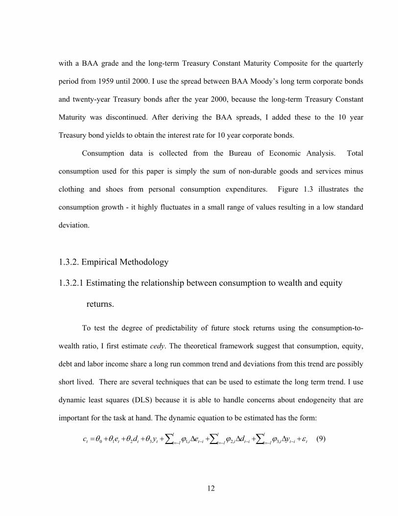
important for the task at hand. The dynamic equation to be estimated has the form:

tl

li itil

li itil

li ititttt ydeydec εϕϕϕθθθθ +Δ+Δ+Δ++++= ∑∑∑ −= −−= −−= − ,3,2,13210 (9)

13

The residuals from equation (9) represent the deviations of the long-term trend estimated

by the cointegrating equation above. These deviations equal to my consumption measure, cedy.

After obtaining cedy, I calculate out-of-sample and in-sample estimates of future stock returns.

For the in-sample regression, the whole sample period is used and the parameters estimated will

determine the fitted values for stock returns, which are compared to the realized returns.

Many researchers argue that in-sample estimates possess a look-ahead bias. Thus, I

perform out-of-sample predictions to overcome this problem. The out-of-sample regressions start

with an initial sample of 65 observations; I then calculate cedy and relate it to the h-period-ahead

stock return. I continue this process, by expanding the sample used in regressions by one

observation at a time until the end of the sample period. Diebold and Mariano (1995) tests are

conducted to assess the statistical significance of these out-of-sample predictions.

1.3.2.2 Estimating conditional risk aversion

Equation (8) has been the subject of numerous tests in financial literature where tα is

replaced by its time invariant counterpart α (Campbell et al (1997)). However, as Figure 1.4

suggests, the price of consumption risk is possibly not stable over time. Thus, a proper estimation

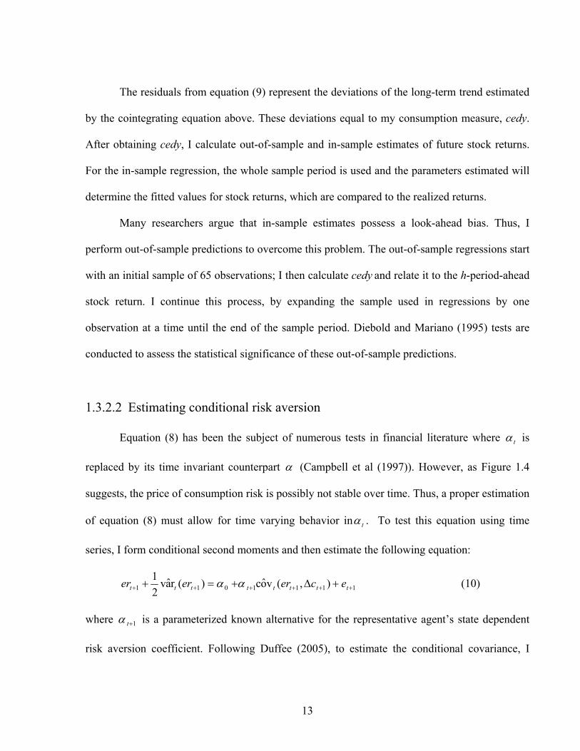
of equation (8) must allow for time varying behavior in tα . To test this equation using time

series, I form conditional second moments and then estimate the following equation:

1111011 ),(voc)(rav21

++++++ +Δ+=+ tttttttt ecererer αα (10)

where 1+tα is a parameterized known alternative for the representative agent’s state dependent

risk aversion coefficient. Following Duffee (2005), to estimate the conditional covariance, I

14

compute period-t+1 excess stock returns and consumption growth as sums of one-step-ahead

expectations and innovations,

1,11 +++ += terttt erEer ε

and (11)

1,11 +++ +Δ=Δ tcttt cEc ε

The product of innovations obtained from equations (11) equals the conditional covariance. It is

impossible to know the true innovations or the information sets that investors rely on. Therefore,

I have to construct fitted residuals based on known information as substitutes for true

innovations. These fitted residuals depend on a set of ex-post variables that serve as my

information set at time t and are my independent variables for the equations below. This set of

variables is carefully described in section 1.3.2.3. The regressions for returns and consumption

growth can be expressed as,

1,1 ' ++ += terrtrt Zer εβ (12)

1,1 ' ++ +=Δ tcctct Zc εβ (13)

where rβ and cβ are parameter vectors and the vectors Zr,t and Zc,t are realized in period t or

before. As in Duffee (2005), I call the set of equations (12) and (13) the zero-stage regressions.

The product of the residuals from the equations above is equal to the ex-post conditional

covariance between consumption growth and stock returns. It is important to note, that I am

interested in the expected conditional covariance as applicable in equation (10). I assume that

this conditional covariance can be represented in parametric form on a set of ex-post

instrumental variables, Xt, in the following regression,

111 '),(cov +++ +=Δ ttttt Xcer υω (14)

15

The ex-post instrumental variables, Xt, are also described in section 1.3.2.3. Once I estimate

equation (14) I arrive to an expected conditional covariance given by,

tttt Xcer 'ˆ),(voc 11 ω=Δ ++ (15)

Equation (15) embodies the first-stage regression; while the following equation

represents the second-stage regression,

11121011 ),(voc)()r(av21

+++++ +Δ++=+ ttttttt cerserer μααα (16)

The second component on the left side is an ex-post estimate of the variance of stock

returns that equals the square fitted residuals from equation (12), 21,1 )ˆ()r(av ++ = terter ε . Equations

(14) and (16) are estimated in a single step using the generalized method of moments (GMM) of

Hansen (1982). GMM is useful since it does not force us to make any assumption about

distributions of returns and errors. As well, it is flexible in the use of several instruments and

restrains residuals to be orthogonal with instruments chosen.

Our main interest lies on the right hand side of equation (16). Specifically, the estimated

parameters that proxy the conditional price of consumption risk (the risk aversion coefficient):

tt s211 ααα +=+ (17)

The term st reflects time variation in the investor’s volition to bear consumption risk. Due

to the number of instruments – there are more moment restrictions than coefficients to estimate –

moments may overidentify the coefficients and some moment restrictions may be inappropriate.

Hansen (1982) “J” tests are required to test if the GMM regression is correctly specified. In

addition, a likelihood ratio test variation for GMM developed by Newey and West (1987b),

called the D-test, is needed in order to test the statistical significance of a time-varying

component in the risk aversion coefficient.

16

1.3.2.3 Choice of instrumental variables The vectors Zr,t and Zc,t are instrument vectors that are used in equations (12) and (13).

The instrument vector Zc,t is used to construct fitted consumption growth residuals, and Zr,t, is

used to construct fitted stock return residuals. I follow Duffee’s choice of instruments for these

equations and include in Zc,t a constant term and a one-period lagged quarterly consumption

growth term. This minimizes the autocorrelation problems found in consumption growth. The

vector Zr,t includes a constant and my consumption–to-wealth ratio, cedy.

The choice of instruments, Xt, for equations (15) and (16) is partly motivated by the

composition effect of wealth noted by Santos and Veronesi (2003). The first instrument I include

is the ratio of stock market wealth to consumption, this variable has the intuitive appeal that as it

increases, consumption is more tightly tied to the performance of the equity markets and thus I

can expect the conditional covariance to behave accordingly. In addition, to account for the so-

called leverage effects present in stock return volatility –which in turn can affect the conditional

covariance between returns and consumption growth – I include lagged excess returns in Xt.

The composition effect also applies to the several other components of total wealth which

differ from stock wealth. This implication suggests that consumption does not only move with

stock market wealth as most literature has implied, but it also moves due to payments from debt,

real estate or labor5. Thus, I also include a measure of volatility of market value of debt in the

instruments set. Again, this choice of instrument is motivated by an intuitive notion, as debt

values become more unstable, we may observe higher volatility in expected future consumption

and very possibly create a contagion effect in equity prices6.

5 In the present study I am only concerned with the impact that debt has on stock returns, therefore real estate is not considered. 6 The events related to credit problems on summer 2007 seem to validate this story as great uncertainty in debt values was reflected as major swings in equity prices.

17

1.4. Empirical Results

This section contains the empirical results. I first provide results on the relationship

between consumption-to-wealth ratio and stock returns. I show that the consumption to wealth

ratio improves the predictability of multi-period-ahead stock returns because of a more thorough

segregation of the net wealth (discussed in Section 1.4.1). Section 1.4.2 contains the results on

the risk aversion coefficient. Cedy confirms the existence of a time-varying component in risk

aversion.

1.4.1 Consumption-to-Wealth ratio and expected future stock returns

I first outline the behavior of the consumption-to-wealth ratio and its relationship with

equity returns. I then test the in-sample and out-of-sample performance of cedy on future equity

returns.

1.4.1.1 Estimates of consumption to wealth ratio and its relationship with stock

returns

Values of cedy represent deviations of the consumption to wealth ratio from its long run

trend. Thus, cedy may contain relevant information regarding revisions about expectations of

future equity returns. From section 1.3.2.1, the parameters for the dynamic equation (9) are

estimated using quarterly data from the first quarter of 1959 to the fourth quarter of 2006 and

yield the following7,

7 For equation (18) l=4. I specified different values for the parameter l, which controls the leads and lags of regression (17), results were mainly unaffected by the choice of lag length.

18

tttt ydec)53.44()82.4()58.8()18.13(

76.003.005.048.1 +++= (18)

The estimated residuals from equation (18) are equivalent to the values for cedy. Newey-West

adjusted t-statistics are displayed in parenthesis below each coefficient of equation (18). Figure

1.5 gives an idea about the performance of cedy over time and illustrates that the relation

between consumption and wealth is stable over the years. As robustness check, I perform

several unit root tests to confirm that cedyt is I(0). The Augmented Dickey Fuller test statistic is -

3.75 and significant at the 1% level, while the Kwiatkowski-Phillips-Schmidt-Shin test statistic is

0.19 and cannot reject stationarity even at the 10% level. This also implies that the linear relation

between consumption and wealth is mirrored by the stable pattern of returns to components of

wealth and consumption growth shown in equation (7).

Remark 1: Cedy values are stationary and represent deviations from the long-term common trend among consumption, equity, debt and labor income. This is analogous to the idea that Cedy values correspond to short-run deviations on returns to wealth.

Next, I use the estimated values of cedy and perform in-sample and out-of-sample tests

and comparisons. This examination sheds light on the importance of separating more thoroughly

the net wealth into its different components.

1.4.1.2 In-sample performance of cedy

To evaluate the in-sample performance of cedy, I run OLS regressions where one-period

ahead returns on the S&P 500 index are regressed against different explanatory variables. As

means of comparison with cedy, I also use Lettau and Ludvigson (2001a) measure cay, the

dividend to price ratio and the dividend to earnings ratio. The last two measures are included

19

because the extant evidence suggests that they possess forecasting power on stock returns, albeit

at very long horizons (Campbell and Shiller (1988) and Fama and French (1988)). Table 1.2

shows a set of estimates resulting from the use of my lagged trend deviation, cedy, and other

lagged variables of interest as independent variables. The table reports in-sample OLS estimates

of the S&P 500 Index real returns and excess returns. For each regression, I correct for serial

correlation and heteroskedasticity in standard errors using the Newey-West (1987) method.

Panel A and panel B show two sets of regressions that differ only in their choice of

dependent variables. On the one hand, panel A reports results using real stock returns as the left-

hand side variable; while on the other hand and for robustness check, panel B reports the

outcome of regressions using real excess returns as the dependent variable. The parameters of

each regression are estimated using the whole sample data.

The first row in panel A reports a regression using a one-period lagged real returns of the

S&P 500 index as independent variables. Results in row 1 show minimum or no explanatory

power over the dependent variable, having an adjusted R2 of zero. In contrast, row 2 and 3 in

panel A, suggest that the use of cay or cedy as independent variables generate superior outcomes,

both with an adjusted R2 of 7%. An interesting conclusion from Table 1.2, is that the dividend

ratios have a seemingly poor effect on real returns over a one-quarter-period; their respective

adjusted R2 is almost or equal to zero. Past literature has accounted for a statistically significant

predictive power that dividend to earnings or prices have on future stock returns (Fama and

French (1988)). My results show that, at least for the case of in-sample short horizons, the

dividend ratios do not contribute much to the explanation of variation in future stock returns. In

addition, I show that these measures do not have the power to subsume the effect that cay or cedy

have on one-period-ahead equity returns; this is revealed in rows 6 and 7 in panel A.

20

Finally, in row 8 and 9 I regress the one-period-ahead returns on all non-consumption

variables (dividend ratios and the lag of the dependent variable) simultaneously with either cay

(row 8) or cedy (row 9). The inclusion of these non-consumption variables actually worsens the

adjusted R2, against using cay or cedy alone, due to the penalty of adding insignificant variables

to the regression. Panel B shows qualitatively similar results relative to panel A.

Remark 2: Cedy provides statistically significant results while explaining in-sample one- period-ahead real and excess returns.

1.4.1.3 Out-of-sample forecasts

This sub-section describes the results for out-of-sample forecasting regressions and tests

using cedy and the other variables introduced in the previous sub-section. The motivation for

this out-of-sample exercise is to avoid the look-ahead bias pertaining to the in-sample

regressions, where some variables may find significant in-sample power explaining future

returns but this power disappears completely when using out-of-sample measures.

Table 1.3 reports a set of results for multi-period-ahead forecast comparisons using the

lagged trend deviation, cedy, as my benchmark. The table reports increasing-window OLS

regression estimates on the predictability of the S&P 500 Index returns. For every single

regression, I corrected for serial correlation and heteroskedasticity in standard errors with the

Newey-West (1987) method.

Each column in Table 1.3 depicts a comparison of predictive models between cedy and

the alternative measures. The different and alternative models, in sequence, utilize either cay,

dividend ratios, term structure of interest rates, short term interest rates or a constant return as

predictive measures, all at time t. There is substantial evidence that expected returns are not

21

constant (Campbell et al (1997)), however, as a basis for comparison it may be useful to contrast

the results derived from using cedy as a forecasting measure against the simplest possible model

such as the constant return model. Since Campbell (1987) found evidence that term structure of

interest rates has predictive power on stock returns, I also included the term structure of interest

rates, trm, and short term interest rates, short, as alternative predictive factors. The term structure

is the difference between the 10 year Treasury bond yield and the three month Treasury bill

yield. The short term interest measure is simply the three month Treasury bill minus its previous

year average; Campbell (1987) called this measure a stochastically detrended interest rate.

The first column in Table 1.3 represents the forecasting horizon in quarters. For example,

h=8 means that the forecast is being estimated two years (8 quarters) forward. To test the

accuracy of the forecasting models, I use the mean square forecasting error (MSFE) as the loss

function and the Diebold-Mariano (1995) test to determine which model performs the best. To

easily compare among models I divide the MSFE estimated when using cedy by the MSFE

estimated from the alternative models; this equals to MSFEcedy/MSFEalternative (MSFE ratio

onwards). Thus, a MSFE ratio that is less than unity means that the mean square forecast error

from the model using cedy is lower than that of the alternative model, confirming the superiority

of the cedy model. The Diebold-Mariano (1995) procedure tests the null hypothesis that two

models have equal predictive power –more properly, it tests that the forecast errors from two

competing models are about the same; in my case, a rejection of this hypothesis represents

statistical evidence in favor of the higher forecasting ability of cedy 8.

Few simple steps are required to estimate the out-of-sample regressions. First, I estimate

equation (9) applying a DLS technique within the estimation period. The initial quarterly

8 I follow Harvey, Leybourne and Newbold (1998) and correct for serial correlation in the Diebold-Mariano statistic; for this I use the Newey-West procedure.

22

estimation period starts from the second quarter of 1959 to the fourth quarter of 1974. The

residuals of this regression equal my consumption-to-wealth measure, cedy. Second, I exclude

the last observation from the cedy series (e.g. fourth quarter of 1974) and perform an OLS

regression of h-period stock returns against the remaining values of cêdy (e.g. from second

quarter of 1959 to the third quarter of 1974). I then record the parameters from this model. Third,

I use the coefficient of cêdy from step two and multiply it by the previously excluded observation

of cêdyt (in this case the 4th quarter of 1974). This product equals the forecast of equity returns h

periods into the future. I record this prediction and estimate the square forecast error. The

process is updated one observation at a time until the fourth quarter of 2006. Finally, the mean

square forecast error is calculated.

In almost every case shown in Table 1.3, the forecasting power of cedy is superior to the

one of alternative measures. In most instances, the MSFE ratio is below unity and the Diebold-

Mariano test rejects at a very high significance level the null hypothesis that the alternative

measures have as much predictive power as cedy. There are a couple of cases where the average

forecasting error from the cedy model is marginally worse compared to other alternative models

(e.g. constant and cay, in horizon 1 and 16 respectively). However, this relation disappears as

horizons change. It is interesting to note that the constant return model seems to be the second

best alternative to the cedy model at shorter horizons, underscoring the difficulty of generating

short to medium horizon out-of-sample forecasts that can improve upon a simple mean.

Another important result is that in almost all cases, as the forecasting horizon increases,

the forecasting power of cedy outperforms that of the alternative measures. These results

implicate cedy as an important predictor of expected future stock returns; the Diebold-Mariano

test gives strong statistical evidence of the superiority of cedy compared to usual benchmarks.

23

Remark 3: Results suggest that cedyt can provide statistically significant and superior predictions on future stock returns for different horizons ahead compared to usual benchmarks.

1.4.2 Risk aversion coefficients

Results from the previous section suggest that cedyt provides significant information

regarding future stock returns. In particular investors revise their willingness to hold risky assets

using cedy or an equivalent measure in their information set. If this is true, we should observe a

time-varying component in risk aversion which may be captured by cedy. Hall (2001) argues

that the increased use of debt as a source of funding over the past few decades makes it difficult

to imagine that equity holdings and human capital represent the entire flow of returns on total

wealth. Thus, total wealth should reflect time varying changes in leverage too.

To estimate the price of consumption risk and test its time dependence I use equation

(16), reproduced below for convenience,

11121011 ),v(oc)()r(av21

+++++ +Δ++=+ tttttt cerserer μααα

where ts2α represents the time dependent component in risk aversion and 1α represents its fixed

component.

There are several theoretical models that employ equation (15) or an equivalent one

(Campbell and Cochrane (1999) and Constantinides (1990)), however extant tests of equation

(16) are few, most notably Duffee (2005), and most find none or weak evidence in favor of time

variability of the price of consumption risk. I estimate equation (16) using the GMM method of

Hansen (1982). I utilize cedy at time t as a proxy for the time-varying component, st, in (16). As

a robustness check I also estimate (16) using the dividend to price ratio (dt – pt) and Wachter’s

(2002) measure of surplus consumption. As substitutes for st, I consider the dividend to price

24

ratio since empirical evidence suggests this measure possesses forecasting power on returns over

long horizons, and I also include Wachter’s surplus consumption measure since it arises naturally

in habit formation models.

As mentioned in section 1.3, the instrument’s set used for the GMM estimation include

the market equity to consumption ratio, a one period lagged excess return, the square of the

return on debt as a measure of volatility in debt returns, and the proxy for time variation in risk

aversion, st, for each case. Due to the number of moment restrictions that overidentify the

coefficients, GMM estimation is carried out in the usual two step procedure, where the first step

uses an identity matrix as the weighting matrix and the second step uses the Newey-West

(1987b) weighting matrix.

Table 1.4 reports the coefficients of the components that form the price of consumption

risk for the different proxies used. In addition, the t-statistics, derived using the delta method,

are presented in parenthesis. Unlike previous empirical research on time variation of risk

aversion, I find significant evidence of a time dependent component in the price of risk. Table

1.4 implies that cedy is the only variable capable of capturing statistically significant time

variation in risk aversion. The coefficient for cedy has the appropriate sign; as shown in figure

1.5, cedy is countercyclical to the business cycle, similar to expected equity returns (Cochrane

(2005)). Therefore for high values of cedy the price of consumption risk must also be high.

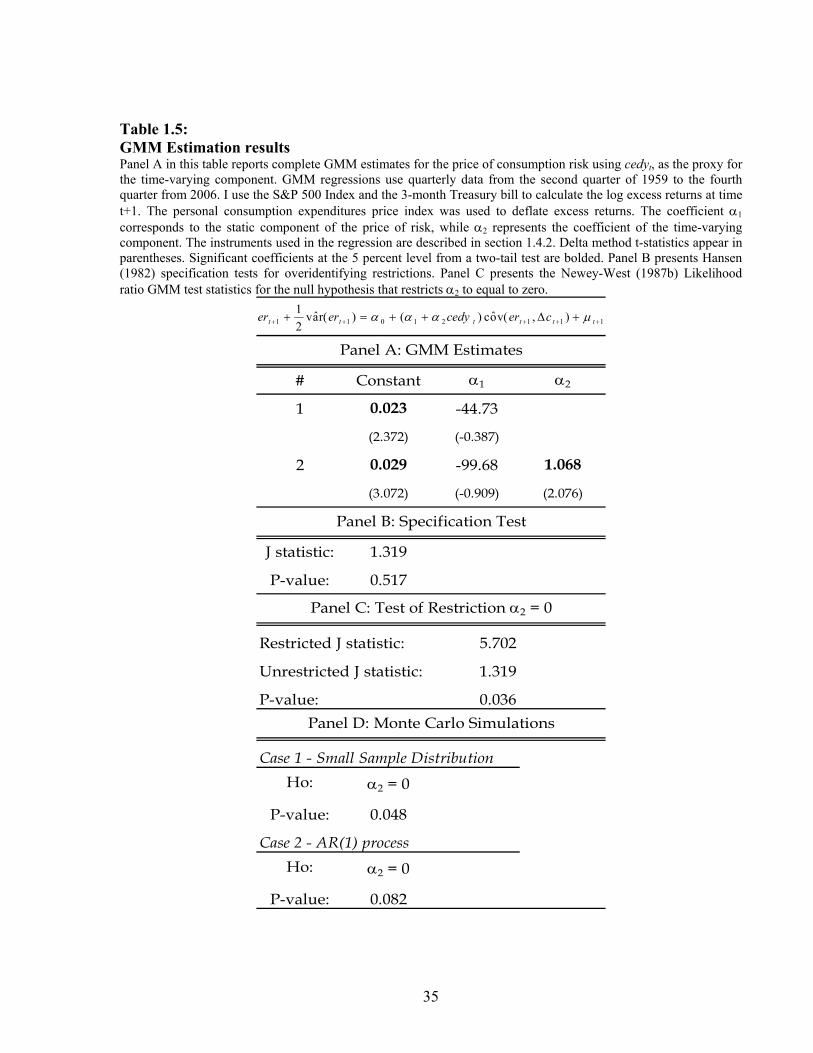
The full estimation results for equation (16) using cedy are presented in Table 1.5. Panel

A shows the parameter estimates. The first row in panel A presents a regression with the

restriction 02 =α , that is imposing time invariance in the risk aversion coefficient, while row 2

presents an unrestricted estimation; again, t-statistics are derived using the delta method and are

25

presented in parenthesis. Overall, results in panel A validate the choice of using cedy as a

measure of time variation in risk aversion.

Panels B and C in Table 1.5 present two different tests for equation (16). Due to the

number of instruments, there are more moment restrictions than coefficients to estimate, thus

moments overidentify the coefficients and some moment restrictions may be inappropriate.

Hansen (1982) developed a specification test for overidentifying restrictions, the “J” statistic of

this test is presented in Panel B along with its p-value derived from a 2χ distribution with

degrees of freedom equal to the number of excess restrictions. Evidence in this table is in favor

of not rejecting the null hypothesis that the unrestricted regression is correctly specified.

Panel C presents the likelihood ratio test variation for GMM developed by Newey and

West (1987b), called the D-test. For this test, I first estimate the unrestricted equation –presented

in row 2 in panel A- using its Newey-West weighting matrix and then I estimate the restricted

equation (row 1), where 02 =α , using the exact same values inside the Newey-West weighting

matrix obtained from the unrestricted version of the model (row 2). Once estimating both

equations with the same Newey-West weighting matrix, I obtain the respective “J” statistics and

calculate the difference between them: the D-test statistic. If the restriction, 02 =α , is

appropriate, the D-test statistic should follow a 2χ distribution with one degree of freedom. The

test rejects such restriction at the 5% significance level. This confirms the evidence in favor of

cedy. Hence, my measure of deviations of consumption-to-wealth ratio captures the time-

variation in the risk aversion coefficient.

26

1.4.3 Robustness Check and Monte Carlo estimations

It is possible that the favorable results obtained for cedy are just the product of incorrect

inference or sheer good luck. After all, cedy may be capturing other elements incorporated in

stock returns that may be unrelated to the risk aversion that investors experience. As a robustness

check for my results, I perform two Monte Carlo experiments; in the first case I check for the

correct inference from the GMM estimators in a finite sample, while in the second case I check

for cedy’s ability to capture a time-varying component in risk aversion that is independent of

cedy. Results of the Monte Carlo robustness tests are presented in panel D, Table 1.5.

Case 1

Since the results from GMM estimation are distributed normal only asymptotically, for

correct inference it’s important to study the small sample properties of the coefficients estimated.

To test if cedy captures the time-varying risk aversion component in equity returns in a sample of

finite size, I construct stock returns that exclude any time-variation in risk aversion (stock-FRA

returns onwards) and then use GMM to estimate equation (16) on this artificial data to check the

empirical distribution of the coefficients.

I first generate 190 one-step-ahead innovations of stock returns and consumption growth

from a multivariate normal distribution with zero mean and covariance matrix that matches the

one of residuals obtained from equations (12) and (13) during the zero stage regressions. I chose

to generate only 190 observations in order to match the number of actual observations that I use

in this paper, from the first quarter of 1959 to the fourth quarter of 2006.

I construct the stock-FRA returns series restricted so excess returns do not possess a time-

varying component,

27

*11,1,

*1

*01,1, ˆ),v(ocˆˆ)r(av

21

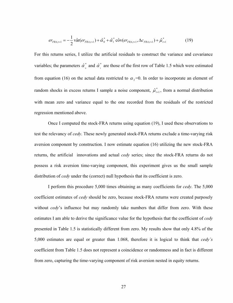
+++++ +Δ++−= ttFRAtFRAtFRAtFRA cererer μαα (19)

For this returns series, I utilize the artificial residuals to construct the variance and covariance

variables; the parameters *0

α and *1

α are those of the first row of Table 1.5 which were estimated

from equation (16) on the actual data restricted to 2α =0. In order to incorporate an element of

random shocks in excess returns I sample a noise component, *1ˆ +tμ , from a normal distribution

with mean zero and variance equal to the one recorded from the residuals of the restricted

regression mentioned above.

Once I computed the stock-FRA returns using equation (19), I used these observations to

test the relevancy of cedy. These newly generated stock-FRA returns exclude a time-varying risk

aversion component by construction. I now estimate equation (16) utilizing the new stock-FRA

returns, the artificial innovations and actual cedy series; since the stock-FRA returns do not

possess a risk aversion time-varying component, this experiment gives us the small sample

distribution of cedy under the (correct) null hypothesis that its coefficient is zero.

I perform this procedure 5,000 times obtaining as many coefficients for cedy. The 5,000

coefficient estimates of cedy should be zero, because stock-FRA returns were created purposely

without cedy’s influence but may randomly take numbers that differ from zero. With these

estimates I am able to derive the significance value for the hypothesis that the coefficient of cedy

presented in Table 1.5 is statistically different from zero. My results show that only 4.8% of the

5,000 estimates are equal or greater than 1.068, therefore it is logical to think that cedy’s

coefficient from Table 1.5 does not represent a coincidence or randomness and in fact is different

from zero, capturing the time-varying component of risk aversion nested in equity returns.

28

Case 2

Constantinides (1990) and Campbell and Cochrane (1999) stated that the time varying

component in risk aversion is related to investor’s habit consumption. They also imply that this

habit follows a pattern that has similarities to an AR(1) process. Therefore, I generate stock

returns (stock-AR returns onwards) that incorporate an AR(1) component as the source for time

variation in risk aversion and check if the success of cedy is due to some independent source of

risk, namely the AR(1) process, that is captured by cedy by just unexpected luck.

I utilize the parameters from row 1 in Table 1.5, artificial innovations of stock returns and

consumption growth and the generated noise component as in the first case to calculate these

stock-AR returns. I include the AR(1) process in equation (16) by replacing ts2α with yt where

tνκ += 1-tt yy and κ is restricted to be randomly and uniformly distributed between 0.05 and

0.95 in order to keep AR(1) process stationary. Notice that yt can reflect persistence in risk

aversion as κ approximates to 0.95 and it is nearly a memoryless process when κ is near to its

lower bound. The following is the stock-AR returns’ equation:

*

11,1,

1,1,*1

*01,1,

ˆ)),v(oc

),v(ocˆˆ)r(av21

+++

++++

+Δ+

+Δ++−=

ttARtAR

tARtARtARtAR

cer

cererer

μ

αα

(y t

(20)

Stock-AR returns do not have a trace of cedy and include an AR(1) component. The

stock-AR returns, the artificial innovations and cedy are used to regress equation (16). I perform

this procedure 15,000 times and generate 15,000 different coefficients for cedy. Replications for

this procedure triple those in case 1 since the AR(1) component adds additional randomness to

the process and to this case. Since stock-AR returns intentionally do not include cedy as a

defining factor, then any of the 15,000 coefficients generated should not be relevant even if by

chance they are different from zero.

29

This experiment gives the small sample distribution for the (correct) null hypothesis that

the coefficient of cedy from equation (16) is insignificant when the time-varying risk aversion is

caused by a process independent of cedy. The significance value for the coefficient of cedy

estimated from equation (16) on actual data, presented in Table 1.5, is 8.23%. This p-value

seems reasonable considering all the amount of uncertainty and randomness in the Monte Carlo

experiment, thus I can be fairly confident that cedy’s coefficient is significant, and its value has

not been determined by randomness but due its ability to capture time-varying risk aversion in

equity returns.

1.5. Conclusions

This article provides evidence on the importance of considering market value of debt in

explaining the relationship between consumption, wealth and equity returns. I develop a

measure of the consumption-to-wealth ratio that accounts for debt values and then relate this

measure to equity returns. The components of wealth include market value of debt, equity and

human capital. I estimate the extent to which inclusion of debt improves the correlation

between this consumption-to-wealth ratio and expected future stock returns. I show that

deviations to this broader measure of consumption-to-wealth ratio, denoted cedy in this article,

can provide statistically significant predictions on future stock returns for different horizons that

surpass other benchmarks. In almost every case tested, the predictive power of cedy is superior

to the one corresponding to alternative factors.

I find statistically significant evidence in favor of a time-varying component in the risk

aversion of investors. The coefficient for cedy has the appropriate sign and supports the notion

that cedy is countercyclical to the business cycle, similar to expected equity returns (Cochrane

30

(2005)); for high values of cedy the price of consumption risk must also be high. Overall, this

evidence points to the importance of considering a more comprehensive definition of wealth

when considering its relationship with equity returns.

31

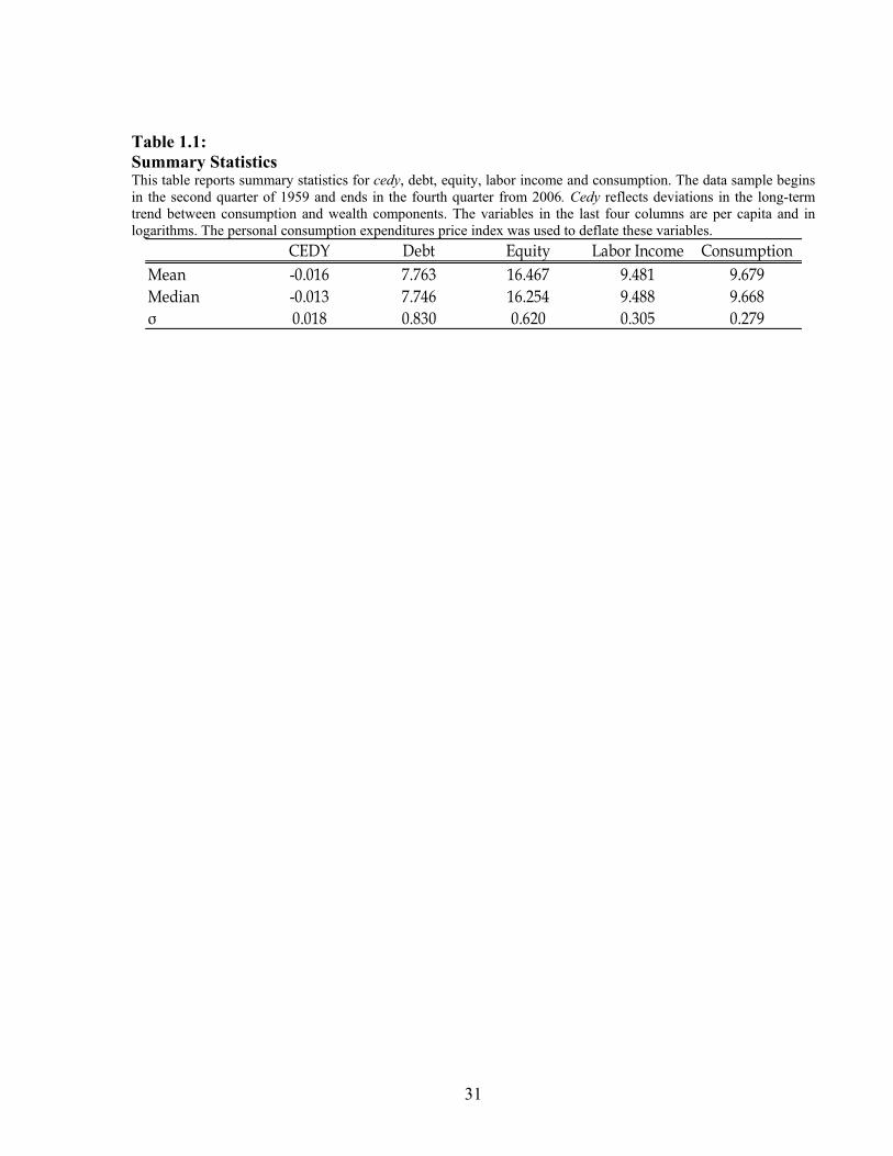
Table 1.1: Summary Statistics This table reports summary statistics for cedy, debt, equity, labor income and consumption. The data sample begins in the second quarter of 1959 and ends in the fourth quarter from 2006. Cedy reflects deviations in the long-term trend between consumption and wealth components. The variables in the last four columns are per capita and in logarithms. The personal consumption expenditures price index was used to deflate these variables.

CEDY Debt Equity Labor Income ConsumptionMean -0.016 7.763 16.467 9.481 9.679Median -0.013 7.746 16.254 9.488 9.668σ 0.018 0.830 0.620 0.305 0.279

32

Table 1.2: Predictability of Stock Returns The table reports estimates from OLS regressions of stock returns on lagged variables. Regressions use quarterly data from the second quarter of 1959 to the fourth quarter from 2006. I use the S&P 500 Index to calculate real returns and excess returns at time t+1 as dependent variables for panel A and B, respectively. The independent variables used were a one period lag of the dependent variable, the trend deviation estimates cayt and cedyt and the log dividend ratios, dt.-et and dt.-pt. The 3-month Treasury bill was used to calculate the log excess returns, while the personal consumption expenditures price index was used to calculate real returns. Newey-West corrected t-statistics appear in parentheses. Significant coefficients at the 5 percent level from a two-tail test are bolded.

# Constant lag cay t cedy t d t - p t d t - e t

1 0.010 0.063 0.00(1.815) (1.068)

2 0.010 1.423 0.07(1.830) (3.428)

3 0.030 0.962 0.07(3.908) (3.067)

4 0.000 0.031 0.02(0.007) (0.857)

5 0.002 0.006 0.00(0.115) (0.470)

6 0.009 1.417 0.002 0.07(0.611) (3.425) (0.062)

7 0.022 0.946 0.022 0.06(1.448) (2.99) (0.586)

8 0.028 0.087 1.554 0.022 -0.019 0.06(1.401) (1.558) (3.751) (0.573) (-1.394)

9 0.015 0.061 0.951 0.020 0.005 0.06(0.759) (1.190) (3.244) (0.459) (0.346)

10 0.006 0.052 0.00(1.149) (0.929)

11 0.006 1.345 0.06(1.060) (3.356)

12 0.023 0.841 0.05(3.031) (2.773)

13 -0.003 0.025 0.00(-0.166) (0.670)

14 0.000 0.005 0.00(0.034) (0.380)

15 0.007 1.353 -0.003 0.05(0.433) (3.443) (-0.069)

16 0.017 0.828 0.017 0.04(1.114) (2.734) (0.440)

17 0.023 0.076 1.482 0.016 -0.018 0.05(1.777) (1.432) (3.674) (0.419) (-1.248)

18 0.011 0.055 0.839 0.015 0.005 0.04(0.524) (1.062) (2.965) (0.344) (0.331)

Panel A: Real Returns; 2Q 1959 - 4Q 2006

Panel B: Excess Returns; 2Q 1959 - 4Q 2006

2R

33

Table 1.3: Out-of-Sample Forecasts of Stock Returns This table reports the results for a multi-period ahead forecast comparisons. The dependent variable is the excess return on the S&P 500 Index at time t+1. Each case represents a comparison between two models, where the cedy model is always being tested. The ratios of the root-mean square forecasting error (MSFE) of the cedy model to the alternative model are reported in columns two to seven. Cedyt is at time t. The models denoted as constant, cayt, dt.-pt, dt.-et, trmt, and shortt, are simply the forecasting models of the stock returns using a constant, and the time t variables of cay, dividend yield, dividend payout, term structure of interest rates, and short term interest rates, respectively. The initial quarterly estimation period starts from the second quarter of 1959 to the fourth quarter of 1974. Then, the model is increasingly re-estimated until the fourth quarter of 2006. The first column corresponds to the forecast horizon, which represents the lags (also corresponding subscript t of the independent variables) of the independent variables and increases in quarters. Diebold-Mariano (1995) test according to the Harvey, Leybourne and Newbold (1998) adjustment were estimated. The null hypothesis of equality of forecasts is rejected at 10%, 5% or 1% significance level if the estimate below comes with: *,**,or ***, respectively.

cedy t vs. cay t cedy t vs. d t - p t cedy t vs. d t - e t cedy t vs. trm t cedy t vs. short t cedy t vs. constant

h = 1 0.958*** 0.934*** 0.955*** 0.950*** 0.953*** 1.002***h = 4 0.860*** 0.822*** 0.876*** 0.938*** 0.856*** 0.923***h = 8 0.877*** 0.713*** 0.803*** 0.872*** 0.810*** 0.823***

h = 12 0.972* 0.710*** 0.722*** 0.813*** 0.733*** 0.737***h = 16 1.002*** 0.683*** 0.684*** 0.807*** 0.683*** 0.685***h = 20 0.960*** 0.682*** 0.684*** 0.825*** 0.659*** 0.665***

MSFEcedy / MSFEalternativeForecast Horizon h

34

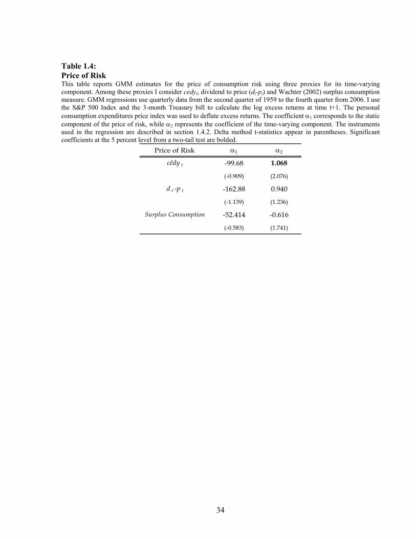
Table 1.4: Price of Risk This table reports GMM estimates for the price of consumption risk using three proxies for its time-varying component. Among these proxies I consider cedyt, dividend to price (dt-pt) and Wachter (2002) surplus consumption measure. GMM regressions use quarterly data from the second quarter of 1959 to the fourth quarter from 2006. I use the S&P 500 Index and the 3-month Treasury bill to calculate the log excess returns at time t+1. The personal consumption expenditures price index was used to deflate excess returns. The coefficient α1 corresponds to the static component of the price of risk, while α2 represents the coefficient of the time-varying component. The instruments used in the regression are described in section 1.4.2. Delta method t-statistics appear in parentheses. Significant coefficients at the 5 percent level from a two-tail test are bolded.

Price of Risk α1 α2

cêdy t -99.68 1.068

(-0.909) (2.076)

d t -p t -162.88 0.940

(-1.139) (1.236)

Surplus Consumption -52.414 -0.616

(-0.583) (1.741)

35

Table 1.5: GMM Estimation results Panel A in this table reports complete GMM estimates for the price of consumption risk using cedyt, as the proxy for the time-varying component. GMM regressions use quarterly data from the second quarter of 1959 to the fourth quarter from 2006. I use the S&P 500 Index and the 3-month Treasury bill to calculate the log excess returns at time t+1. The personal consumption expenditures price index was used to deflate excess returns. The coefficient α1 corresponds to the static component of the price of risk, while α2 represents the coefficient of the time-varying component. The instruments used in the regression are described in section 1.4.2. Delta method t-statistics appear in parentheses. Significant coefficients at the 5 percent level from a two-tail test are bolded. Panel B presents Hansen (1982) specification tests for overidentifying restrictions. Panel C presents the Newey-West (1987b) Likelihood ratio GMM test statistics for the null hypothesis that restricts α2 to equal to zero.

# Constant α1 α2

1 0.023 -44.73

(2.372) (-0.387)

2 0.029 -99.68 1.068

(3.072) (-0.909) (2.076)

J statistic: 1.319

P-value: 0.517

Restricted J statistic: 5.702

Unrestricted J statistic: 1.319

P-value: 0.036

Case 1 - Small Sample DistributionHo: α2 = 0

P-value: 0.048

Case 2 - AR(1) processHo: α2 = 0

P-value: 0.082

Panel A: GMM Estimates

Panel B: Specification Test

Panel C: Test of Restriction α2 = 0

Panel D: Monte Carlo Simulations

11121011 ),v(oc)()r(av21

+++++ +Δ++=+ tttttt cercedyerer μααα

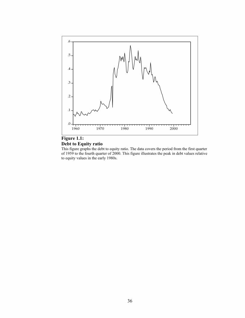
36

.0

.1

.2

.3

.4

.5

.6

1960 1970 1980 1990 2000

Figure 1.1: Debt to Equity ratio This figure graphs the debt to equity ratio. The data covers the period from the first quarter of 1959 to the fourth quarter of 2000. This figure illustrates the peak in debt values relative to equity values in the early 1980s.

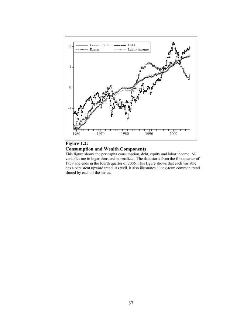
37

-1

0

1

2

1960 1970 1980 1990 2000

ConsumptionEquity

DebtLabor income

Figure 1.2: Consumption and Wealth Components This figure shows the per capita consumption, debt, equity and labor income. All variables are in logarithms and normalized. The data starts from the first quarter of 1959 and ends in the fourth quarter of 2006. This figure shows that each variable has a persistent upward trend. As well, it also illustrates a long-term common trend shared by each of the series.

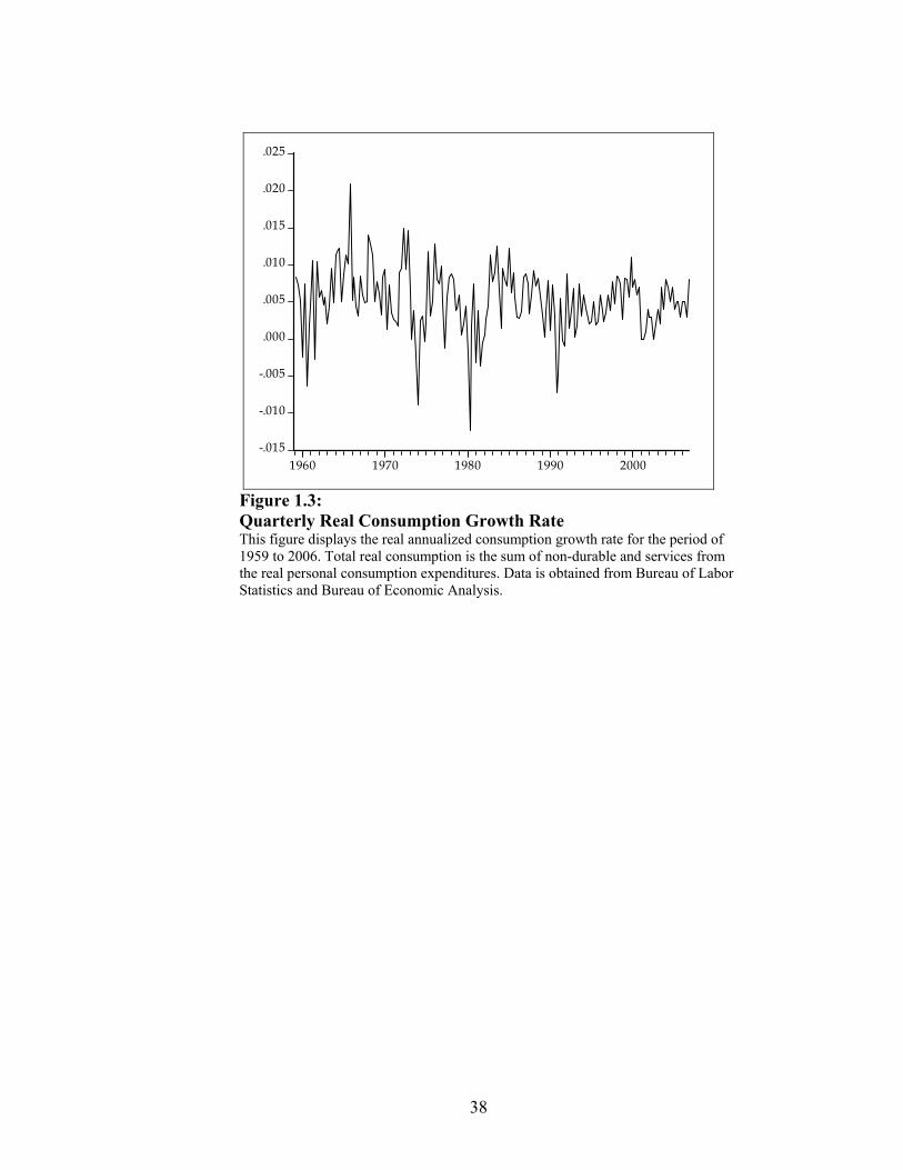
38

-.015

-.010

-.005

.000

.005

.010

.015

.020

.025

1960 1970 1980 1990 2000

Figure 1.3: Quarterly Real Consumption Growth Rate This figure displays the real annualized consumption growth rate for the period of 1959 to 2006. Total real consumption is the sum of non-durable and services from the real personal consumption expenditures. Data is obtained from Bureau of Labor Statistics and Bureau of Economic Analysis.

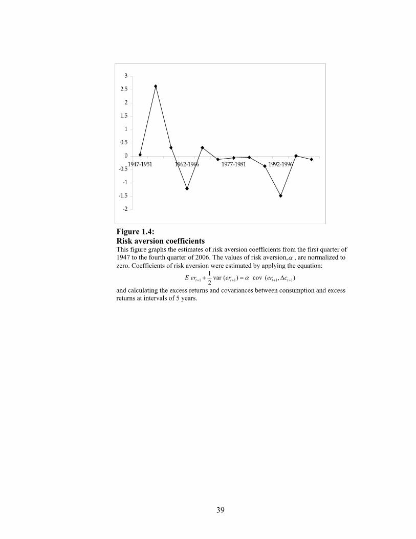
39

-2

-1.5

-1

-0.5

0

0.5

1

1.5

2

2.5

3

1947-1951 1962-1966 1977-1981 1992-1996

Figure 1.4: Risk aversion coefficients This figure graphs the estimates of risk aversion coefficients from the first quarter of 1947 to the fourth quarter of 2006. The values of risk aversion,α , are normalized to zero. Coefficients of risk aversion were estimated by applying the equation: ),(cov)(var

21

1111 ++++ Δ=+ tttt cerererE α

and calculating the excess returns and covariances between consumption and excess returns at intervals of 5 years.

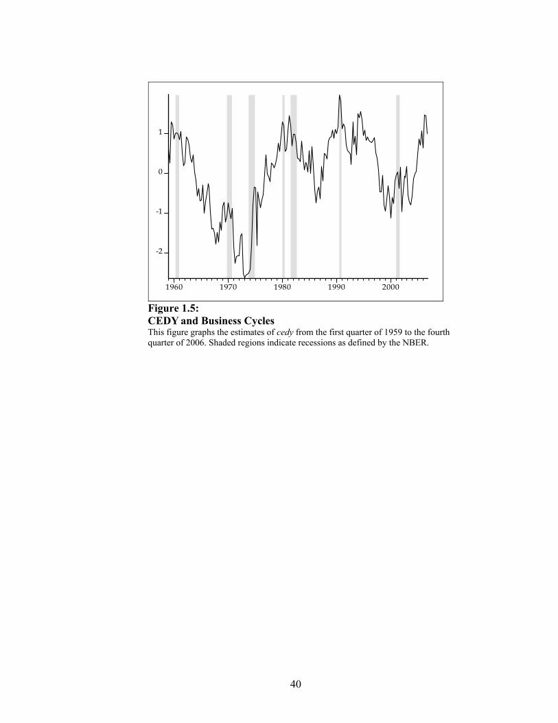
40

-2

-1

0

1

1960 1970 1980 1990 2000

Figure 1.5: CEDY and Business Cycles This figure graphs the estimates of cedy from the first quarter of 1959 to the fourth quarter of 2006. Shaded regions indicate recessions as defined by the NBER.

41

CHAPTER 2: EXPECTATIONS, CONSUMPTION TO WEALTH RATIO

AND EQUITY RETURNS

2.1. Introduction

Finance literature has historically attempted to take theoretical models of consumption

based asset pricing to equity market data. Early ground-breaking works on asset pricing include

Lucas (1978) and Breeden (1979) among others; however, most of these early works only give a

relevant role to payouts from equity. In light of this, recent studies, such as Jagannathan and

Wang (1996), Lettau and Ludvigson (2001a, 2001b), Julliard (2004), Duffee (2005), Piazzesi,

Shneider and Tuzel (2007), have focused on models that include other wealth sources which are

proven to have a substantial effect on asset prices.

The framework presented in this article, shows how consumption and several wealth

components are directly related to discounted future returns to wealth. I segregate wealth into

four components: payments to debt (by lending money and obtaining an interest on the loan),

equity, real estate (housing), and labor income. I use these four variables because, through

history and based on literature findings, they have been considered as the main sources of

wealth. To my knowledge, there is no previous work that has utilized these four wealth sources

together to explain changes in equity returns.

My first contribution in this article is to shed light in the arena of asset pricing by finding

relevancy on using a more thorough wealth segregation to explain movements of equity returns. I

provide a parsimonious framework that connects consumption with the market values of debt,

housing, equity and human capital. My theoretical motivation relies on the work made by

Campbell and Mankiw (1989), Campbell (1996), and Lettau and Ludvigson (2001a).

42

Starting with Lettau and Ludvigson (2001a), previous work argue that deviations from

the long run stable state between consumption and wealth predict future stock returns; I make the

case instead that it is the changes in expectations of the consumption to wealth ratio from one

period to the next one that matters for predicting changes in stock returns.

Thus, my second contribution is to develop a measure of changes in expectations on the

consumption to wealth ratio (I call this variable u-ccw) which is theoretically related to changes

in expected equity returns. I empirically test if this variable outperforms commonly used

measures when explaining future stock returns.

As a third contribution, I estimate the change in expectations of discounted future

consumption growth. When calculating the consumption to wealth ratio, most researchers make

different assumptions about consumption growth and then omit this term in their hypotheses; I

instead include it in my model.

For the empirical tests, I use quarterly observations on financial time-series for the United

States over the period of 1959 to 2006. This data is compiled from CRSP, the Federal Reserve,

the Census Bureau, and the Bureau of Economic Analysis. The value of outstanding equity is

equal to the total market value of NYSE-AMEX-NASDAQ stocks obtained from CRSP

database. Using the Flow of Funds Data, I calculate the market value of debt (explained in

section 2.2.2). I obtain labor data following the work of Ludvigson and Lettau (2001a); whereas

real estate values are constructed following the work of Hasanov and Dacy (2005) and using

NIPA tables. Consumption is defined as nondurables plus services minus shoes and clothing, and

is also taken from the NIPA tables.

My main results are that u-ccw outperforms all of the alternative predictors considered in

this article. I perform Welch and Goyal’s (2003, 2006) graphical analysis that renders evidence

43

in favor for u-ccw as a good predictor of future stock returns. This test shows that, for the greater

part between 1975 and 2006, u-ccw can provide useful information about one-quarter ahead

stock returns. In addition, I find statistically significant evidence in favor of including the

discounted future consumption growth. In asset pricing literature, this term is usually disregarded

for different reasons; I calculate the change in expectations of this variable and find out that it

carries essential information when predicting future stock returns.

2.1.1 Literature review

Since recently, most of the empirical evidence on explaining the relationship between

consumption and equity returns has been built on the assumption that equity returns correspond

to the entire claim on the existing stock of capital (Rouwenhorst (1995)).

Some other empirical work has examined the relationship between aggregate equity

returns and debt using asset pricing models. Empirical evidence supports the idea that business

cycles and changes in default risk (which is directly related to the amount of leverage) may affect

equity returns (e.g., Chen, Roll, and Ross (1986), Keim and Stambaugh (1986), Campbell and

Shiller (1988), Chen (1991), Ferson and Harvey (1991), Jagannathan and Wang (1996), Vassalou

and Xing (2004), Vassalou, Chen and Zhou (2005), Zhang (1997) and Alvarez and Jermann

(2000)).

On the other hand, housing has been little explored in the asset pricing area, even though

housing expenditure has always been a predominant part of the United States’ gross domestic

product. Over the last 50 years, it accounted for more than twenty percent of the economy’s

spending. Recent asset pricing papers that have included housing returns in their analysis are:

44

Piazzesi, Shneider and Tuzel (2007) and Hasanov and Dacy (2005). These papers have found

significant evidence relating housing returns to equity returns.

Finally, the importance of labor income in asset pricing has caught the attention of many

researchers since the pioneering work of Jagannathan and Wang (1996). It is important to

include labor income in the asset pricing analysis; given that, currently, the ratio of labor income

to consumption is close to two thirds. Julliard (2004) analyzed the role of labor income in the

relationship between consumption, wealth and asset returns, and found that labor income plays a

significant part in the explanation of future asset returns.

The article is organized as follows. Section 2.2.2 gives the theoretical background.

Section 2.2.3 describes the data and methodology and Section 2.2.4 contains empirical findings.

Section 2.2.5 concludes.

2.2. Theoretical approach

My objective in this section is to utilize four components of total wealth and link them to

wealth returns. As wealth sources, I include market value of debt, equity, housing, and labor

income into the representative agent’s intertemporal budget constraint. I adapt the framework of

Campbell and Mankiw (1989) and key in the four wealth components in their setting. This

setting allows me to determine how disaggregating wealth will affect equity returns. In section

2.2.1, I demonstrate the steps to arrive at the Campbell and Mankiw’s consumption-to-wealth

ratio model, and I elaborate on the four components of net wealth. In section 2.2.2, I expand

Campbell and Mankiw’s framework and include a more thorough definition of net wealth. I

include the four wealth components separately and show their relation to stock returns.

45

2.2.1 Housing, debt, equity and human capital wealth and their relation to stock

returns

The idea behind disaggregating wealth into several components is to take into account the

impact that each wealth factor has on stock returns separately. I first postulate that when wealth

is separated into several elements, a better explanation to stock return movements can be

obtained. The framework developed in this section draws heavily from Campbell and Mankiw’s

(1989) work.

2.2.1.1 Consumption to wealth ratio

Total wealth in time t, tW , is divided into equity, debt, real estate and human capital; in

other words, I propose that ttttt HCHDEW +++= , where the first two elements of the right-

hand side correspond to the market value of equity and debt respectively, the third component

represents housing or real estate wealth and the fourth element is human capital. Lettau and

Ludvigson (2001a) and Julliard (2004) follow a similar approach but exclude debt and real estate

wealth.

The budget constraint equation between period t and t+1 is written as:

))(1( 1,1 tttwt CWRW −+= ++ (1)

where tC is consumption at time t, and 1, +twR , is the return on the remaining wealth invested in

time t.

Taking logs and using a first order Taylor expansion on equation (1), rearranging terms

and solving forward gives (ignoring the linearization constant) ,

∑∞

= ++ Δ−=−1 , )(

i ititwi

tt crwc ρ (2)

46

Just as in Campbell and Mankiw (1989), the Taylor expansion of equation (1) was

calculated around a steady state, where the average ratio of invested wealth to total wealth,

WCW − , is assumed constant; making

WCW −

=ρ a number smaller than 1. Notice that lower

case letters in this article represents the variables in logarithms.

Equation (2) represents total consumption to total wealth ratio, tt wc − , at time t. While

Campbell and Mankiw use net wealth, tW , in equation (2), I contribute to the finance literature

by instead expressing tW as the sum of its different components: tttt HCHDE +++ .

2.2.2 Modifications to the Campbell and Mankiw (1989) consumption to wealth

model.

This section extends Campbell and Mankiw’s (1989) model by segregating total wealth

and returns to total wealth into four main components. There is evidence relating consumption to

wealth ratio to returns to wealth. However, to my knowledge, no research paper has included the

four wealth components explained in section 2.2.1.

Lettau and Ludvigson (2001a) use a variable that accounts for equity, debt and housing

all together, in other words they use total asset holdings. They proxy for asset holdings by using

the net household worth series provided by the Federal Reserve Board. This measure is noisy

since the Federal Reserve estimates this household net worth series as a residual; that is, for any

particular asset, the Federal Reserve estimates first the participation of other economic agents

and then attributes the rest to households9. Other research papers such as Julliard (2004),

excludes debt as part of wealth. I empirically show that accounting separately and explicitly for 9 The Federal Reserve also bundles households and nonprofit organizations together, so the net worth series is actually a measure of household and nonprofit organizations total wealth.

47

debt, equity, housing, and labor income wealth the correlation between stock return patterns and

the consumption-to-wealth ratio will improve.

2.2.2.1 Disaggregate total wealth and disaggregate returns to total wealth

As mentioned before, I use disaggregated wealth instead of total wealth to explain equity

returns. But in order to incorporate this into the consumption to wealth ratio model, I have to log-

linearize the following: ttttt HCHDEW +++= .

I applied several first orders Taylor expansions, to finally obtain the next log-linearized wealth

equation (I ignore the linearization constant):

ttttt hchdew 4321 ββββ +++= (3)

Log of wealth is now in function of logarithmic wealth components. As well, the beta

coefficients next to the variables are all constant..

Substituting hct for yt, in equation (3) yields the following:

ttttt yhdew 4321 ββββ +++= (4)

Since the consumption-wealth ratio model also includes returns to total wealth, I

therefore have to disaggregate these returns into returns to the main wealth components. Returns

to total wealth take the subsequent form: 1,41,31,21,11, +++++ +++= tYtHtDtEtW RRRRR αααα .

I log-linearize the total return to wealth equation by applying several first order Taylor

expansions around different sets of steady states. I arrive to the equation below (ignoring the

linearization constant),

1,41,31,21,11, +++++ +++≈ tYtHtDtEtW rrrrr αααα (5)

Now, substituting equation (5) and (4) into equation (2), we get:

48

∑∞

= +++++ Δ−+++=

=−−−−

1 ,4,3,2,1

4321

)( i ititYitHitDitE

i

ttttt

crrrr

yhdec

ααααρ

ββββ (6)

The left hand side of equation (6) represents the consumption to wealth ratio when all

components of wealth are taken into account individually. All variables are observable. The right

side of equation (6) corresponds to the separate log returns to each respective wealth component

minus a consumption growth term.

Since all the terms on the right-hand side of equation (6) are presumed stationary, ct, et,

dt, ht, and yt must be cointegrated. The left-hand side of equation (6) gives the deviation in the

common trend of ct, et, dt, ht, and yt. From now on, I denote the trend deviation term

ttttt yhdec 4321 ββββ −−−− as ccw.

Consistent with previous literature, I assume that revisions from one period to the next one on

expected returns to debt, housing and labor income do not change or are stationary.

Campbell and Mankiw (1989), Lettau and Ludvigson (2001a) and Julliard (2004) obtain

a similar expression to equation (6), however they do not account separately for certain

components of asset holdings.

Lettau and Ludvigson (2001a) denoted their trend deviation of consumption, assets and

human capital as cay – where ct, at and yt represent consumption, asset holdings and labor

income, respectively. In future sections, I’ll use cay for comparison purposes.

2.3. Empirical methodology

2.3.1 The relationship between consumption to wealth ratio and equity returns

The theoretical framework suggest that consumption, equity, debt, housing and labor

income share a long run common trend and deviations from this trend are possibly short lived. I

49

use dynamic least squares (DLS) to estimate the cointegrating relation between consumption and

the components of wealth because it is able to handle concerns about endogeneity that are

important for the task at hand. The dynamic equation to be estimated has the form:

t

l

liiti

l

liiti

l

liiti

l

liiti

ttttt

yhde

yhdec

εφφφφ

ββββ

+Δ+Δ+Δ+Δ+

++++=

∑∑∑∑−=

−−=

−−=

−−=

− ,1,1,1,1

4321

. (7)

The residuals from equation (7), tε , represent the deviations of the long-term trend

estimated by the cointegrating equation above.

2.3.2 Vector Error Correction Model, Vector Autoregressive Model, and the

Changes in Expectations of Consumption to Wealth

In this section I analyze the change in expectations of the consumption-to-wealth ratio

and how this relates to the change in expectations to discounted future returns to wealth. To do

this, I will estimate a vector autoregressive model (VAR) and a vector error correction model

(VECM).

Hypothesis 1: Changes in expectations of consumption-to-wealth ratio contain important information when explaining movements in expected stock returns.

Taking expectations at time t on equation (6), the following is true:

( )∑∞

= +++++ Δ−+++=

=−−−−

1 ,4,3,2,1

4321

)(

)(

i ititYitHitDitEi

t

tttttt

crrrrE

yhdecE

ααααρ

ββββ

(8)

Now, if we subtract the expectation of t-1 of equation (6) from equation (8), and rearranging

terms, we get the next equation:

50

).)()((

)())((

1 ,4,3,2,11

1143211

∑

∑∞

= ++++−

∞

=+−−

+++−=

=Δ−+−−−−−

i itYitHitDitEi

tt

iit

ittttttttt

rrrrEE

cEEyhdecEE

ααααρ

ρββββ

(9)

Equation (9) represents the change in expectations of consumption to wealth ratio and

consumption growth, which is in function on the expectations on returns to wealth components.

Notice that expectations at time t of a variable at time t, is simply the realized value of such

variable, in other words ttt ccE = .

Working with the first term of left hand side of equation (9), we have that,

)()()()()()()()()()(

141312111

141312111

ttttttttttttttt

ttttttttttttttt

yEyhEhdEdeEecEcyEEhEEdEEeEEcEE

−−−−−

−−−−−

−−−−−−−−−=−−−−−−−−−

ββββββββ (10)

The betas in the equation above correspond to the cointegrating coefficients from

equation (7) which will be estimated by the DLS method. Equation (10) naturally motivates a

VAR estimation procedure, where we can estimate the change in expectations as innovations at

time t for all of the variables considered in the equation above without imposing functional

assumptions besides linearity.

The VAR approach sidesteps the need for structural modeling by treating every

endogenous variable in the system as a function of the lagged values of all of the endogenous

variables in the system. In this article, to estimate the VAR model, I will use the components of

consumption to wealth ratio as endogenous variables.

Notice that if we let

[ ]′= tttttt yhdecF

Then the corresponding VAR equation with one lag (this is without loss of generality since

higher order VAR systems can be re-expressed as a one lag VAR) is:

tυa ++= −1tt FF θ (11)

51

and we can express equation (10) equivalently as:

[ ] tccwu −=−−−− tυ43211 ββββ (12)

Equation (12) represents the change in expectations in consumption-to-wealth ratio. I

denote this measure as u-ccw for the remainder of the paper.

The second term on the left hand side of equation (9) represents discounted future

consumption growth. When calculating the consumption to wealth ratio, most researchers make

different assumptions about the consumption growth and then omit this term in their hypotheses.

Using the VEC model, I am able to extract information from this previously disregarded term.

Furthermore it will be shown in my results that this term carries important implications when

studying expected stock returns.

Hypothesis 2: Discounted future consumption growth has important implications when studying expected stock returns and should not be disregarded.

To estimate the discounted future consumption growth, I rely on the Granger

Representation Theorem. This theorem states that a cointegrated system can be equivalently

represented as a VECM. Since consumption is cointegrated to wealth components, then their

short term disequilibrium can be expressed in the error correction form. Therefore, due to the

fact that consumption is cointegrated to components of wealth, and following the Granger

Representation Theorem, it is suggested that the following error correction model exists:

tuγ ++= −− 11 ttt ZAZ ε (13)

where [ ]′ΔΔΔΔΔ= tttttt yhdecZ ,

1−tε is the disequilibrium error resulting from equation (7), and γ is (5x1) vector representing the

short run speed of adjustment parameter for each variable in Zt. The disequilibrium error is

52

stationary since consumption and wealth are cointegrated, meaning that short term deviations

from their long run trend are being corrected. This is implied by the VECM.

The VECM was used to calculate the changes in expectations of discounted future

consumption growth. Note that for the VECM in (13) we have that

111

1 −−+

+− += tj

tj

jtt AZAZE εγ (14)

tj

tj

jtt AZAZE εγ1−+ +=

Using the two equations above we have that

( )[ ]

[ ]tjj

j

j

tj

tttj

j

j

tj

tj

tj

tj

j

j

jjttt

j

AA

AZAZA

AZAAZAZEE

ερ

εερ

εερρ

γu

γγ

γγ

t1

1

111

1

1111

111 )()(

−∞

=

−−−

∞

=

−−+−

∞

=

∞

=+−

+=

+−−=

−−+=−

∑

∑

∑∑

Furthermore,

[ ]

( ) ( ) t

tj

j

jj

j

j

tj

j

jj

j

jt

jj

j

j

AIAIA

AAA

AAAA

ερρρρ

ερρρρ

ερρερ

γu

γu

γuγu

t

t

tt

11

1

1

11

1

1

1

11

1

1

−−

−∞

=

−−∞

=

−

−∞

=

∞

=

−∞

=

−+−=

+=

+=+

∑∑

∑∑∑

Now let e1 be the characteristic vector that identifies Δct in Zt, that is,

Δct = e1’ Zt = [ ] tZ00001 , thus

( ) ( )[ ]t

jjttt

j

jjttt

j

AIAIAe

ZEEecEE

ερρρρ

ρρ

γut11

1

111

11 )()(

−−

∞

=+−

∞

=+−

−+−′=

−′=Δ− ∑∑

(15)

The most insightful results in this section give us a new expression for equation (9). Plugging

equation (12) and equation (15) into equation (9), we have that

53

[ ] ( ) ( )[ ]

∑∞

= ++++−

−−

+++−=

−+−′+−−−−

1 ,4,3,2,11

1114321

)()(

1

i itYitHitDitEi

tt

t

rrrrEE

AIAIAe

ααααρ

ερρρρββββ

γuυ tt (16)

The left hand side of equation (16) estimates present revisions about future returns. As

mentioned before, I assume that revisions from one period to the next one on expected returns to

debt, housing and labor income do not change. My assumption is actually weaker than the one

commonly used in the literature, since I do not require that expectations remain constant. Thus,

my assumption only needs expectations to remain roughly the same based on the information

sets at periods t-1 and t. Therefore, we can expect the left hand side to have some predictive

power over next period returns. Based on this, the equation needed to estimate in-sample and

out-of-sample regressions is the following,

(16a)

where, on the right hand side, the first term is a constant, the second term is simply u-ccw, the

third term is the discounted future consumption growth and the last term is an error.

2.4. Empirical Results

Section 2.4.1 presents the results for the cointegrating equation (7). Section 2.4.2 includes

the changes in expectations of consumption-to-wealth ratio (in this case: the u-ccw). Section

2.4.3 contains the results on in-sample and out-of-sample performance of u-ccw. Section 2.4.4

includes Campbell and Yogo (2006) size distortion tests on in-sample regressions and the Welch

and Goyal (2003, 2006) plot/test for performance on out-of-sample forecasts models.

[ ]( ) ( )[ ] 1

1113

4321211, 1

+−−

+

+−+−′+

+−−−−+=

ttt

ttE

AIuAIAe

r

τεγρρρρϕ

υββββϕϕ

54

When empirically testing the consumption to wealth ratio’s ability to predict future stock

returns, previous works such as Lettau and Ludvigson (2001a) and Julliard (2004) have used a

two step procedure. In the first step, the residuals from the cointegrating equation of

consumption and wealth are estimated, and, in the second step, these estimated residuals are used

as explanatory variable in an OLS regression predicting future stock returns. It is well known in

the econometrics literature that using estimated values as explanatory variables may lead to

incorrect standard errors that do not take into account the uncertainty associated with the

estimated explanatory variable.

In the present case, I estimate the cointegration model, and use the residuals from this

regression in the VEC model (equation (13)). Furthermore, I use a linear combination of the DLS

coefficients the VEC and VAR models’ results to estimate the predictive model outlined in

equation (16). In order to avoid the bias in standard errors, I estimate all equations jointly using

the GMM framework of Hansen (1982)10 as explained in appendix 2.D. An additional benefit of

the GMM procedure is that estimates are robust to common misspecification problems, such as

heteroskedasticity and autocorrelation.

2.4.1 DLS estimates for the Consumption-to-Wealth ratio

From section 2.3.1, the parameters for the dynamic equation (7) are estimated using

quarterly data from the first quarter of 1959 to the fourth quarter of 2006 yielding the

following11,

10 Results are presented for efficient GMM, using a Newey-West weighted matrix. Point estimates are the same using and identity weight matrix. 11 For equation (17) l=1. I specified different values for the parameter l, which controls the leads and lags of regression (7), results were mainly unaffected by the choice of lag length.

55

ttttt hydec)46.15()51.19()97.3()54.10()46.15(

12.066.002.004.034.1 ++++= (17)

I perform several unit root tests to confirm that residuals from equation (7) are I(0). The

Augmented Dickey Fuller test statistic is -3.33 and significant at the 1% level, while the

Kwiatkowski-Phillips-Schmidt-Shin test statistic is 0.17 and cannot reject stationarity at the 10%

significance level. This also implies that the linear relation between consumption and wealth is

mirrored by the stable pattern of returns to components of wealth and consumption growth

shown in equation (6).

As mentioned before, the coefficients of equation (17) are imperative for the estimation

of the changes in expectations of consumption to wealth ratio.

Remark 1: There exists a long-term common trend among consumption, equity, housing, debt and labor income.

2.4.2 VECM, VAR and Changes in Expectations of Consumption to Wealth Ratio

After estimating the cointegrating equation (17), I proceed to estimate u-ccw and the

changes in expectations to the discounted future consumption growth. With the VAR model I

estimated equation (11) and obtained u-ccw as in equation (12); while with the VEC model I

estimated equation (13) and obtained the discounted future consumption growth as depicted in

equation (15).

As will be demonstrated in the following sections, both terms are shown to be relevant

when predicting future stock returns. In sample and out-of sample regressions are estimated

using u-ccw plus the term for discounted future consumption growth.

56

2.4.3 In-sample and Out-of-sample performance

I use the estimated values of u-ccw 12 plus the consumption term (check appendix 2.D for

GMM estimation procedure of these terms), cay, and other predictor variables and perform in-

sample and out-of-sample tests and comparisons. This examination reveals the importance of

separating more thoroughly the net wealth into its different components and of estimating the

change in expectations of consumption to wealth ratio and of the discounted future consumption

growth.

2.4.3.1 In-sample regressions

To evaluate the in-sample performance of u-ccw, the one-period ahead CRSP returns are

regressed against different explanatory variables. As means of comparison with u-ccw, I also use

Lettau and Ludvigson (2001a) measure cay, Quijano’s (2007) cedy, another consumption to

wealth ratio measurement that excludes housing, lagged returns to equity, the dividend to price

ratio, the dividend to earnings ratio and the stochastically detrended short term interest rates. The

last three variables are included because the extant evidence suggests that they possess

forecasting power on stock returns, albeit at very long horizons (Campbell and Shiller (1988) and

Fama and French (1988)). Table 2.4 shows a set of in-sample estimates resulting from the afore

mentioned variables as predictors of CRSP real returns. The parameters of each regression are

estimated using the whole sample data.

Results using lagged returns (row 1) show minimum or no explanatory power over the

dependent variable, having an adjusted R2 of zero. However, row 2 and 3 suggest that the use of

cay or cedy as independent variables generate superior outcomes, both with an adjusted R2 of 5%

12 I only report results for the u-ccw since it outperforms the ccw. However, it is important to note that ccw outperforms the rest of the predictor variables used for comparisons.

57

and 4% respectively. Dividend measures have a seemingly poor effect on real returns over a one-

quarter-period; their respective adjusted R2 is almost or equal to zero. Past literature has

accounted for a statistically significant predictive power that dividend to earnings or prices have

on future stock returns (Fama and French (1988)). My results show that, at least for the case of

in-sample short horizons, the dividend to price ratio and dividend to earnings ratio do not

contribute much to the explanation of variation in future stock returns. On the other hand, it

seems that the stochastically detrended short term interest rates have some in-sample

predictability over stock returns, however their explanatory power is somewhat weak compared

to the other significant models. Finally, row 7 shows the results u-ccw plus the discounted future

consumption growth. Both, u-ccw and the discounted future consumption growth show great

statistically significance in the model. Though the R2 in row 7 is lower compared to the cay or

cedy models, the statistical significance of the coefficients of my predictor variables is

substantially higher. This indicates that consumption growth is an important indicator that cannot

be disregarded when trying to forecast stock returns.

Remark 2: U-ccw and the discounted future consumption growth provide statistically significant results while explaining in-sample one-period-ahead real equity returns.

Results for the Campbell and Yogo’s size distortion test

The results in the previous subsection take for granted the validity of t-tests computed

from a one-period predictive in-sample regressions. However, as discussed in appendix 2.C, it is

possible these t-tests are biased towards spurious rejection of the null hypothesis of no

significance. I estimate the Campbell and Yogo (2006) pretest to check for size distortion in

58

these t-tests, specifically I test as null hypothesis if the 5% size of the t-test is biased and actually

more than 7.5%. Table 2.5 reports the results for Campbell and Yogo’s size distortion test.

Results from this pretest show that the null hypothesis is rejected for u-ccwt and

discounted consumption growth term, thus we can confidently conclude that the evidence in

favor of predictability found in the previous section is not due to biased statistical procedures.

Also, it is worth noting in Table 2.5 that popular measures believed to forecast stock returns,

such as the dividend to price ratio and Ludvigson and Lettau’s cay, actually suffer from size

distortion and it is quite possible that the belief that these variables forecast stock returns is only

due to incorrect inference –Goyal and Welch (2003, 2006) reach a similar conclusion, though for

out-of-sample forecasts.

2.4.3.2 Out-of-Sample Forecasting Regressions

The motivation for this out-of-sample exercise is to avoid the look-ahead bias pertaining

to the in-sample regressions, where some variables may find significant in-sample power

explaining future returns but this power disappears completely when using out-of-sample

measures. Thus, I calculate the performance of out-of-sample forecasts allowing for an

increasing estimation window.

Few simple steps are required to estimate the out-of-sample forecasts. I estimated

equation (7), (11), and (13) and (16a) simultaneously using the GMM procedure explained in

appendix 2.D. With the estimations, I obtained u-ccw and the consumption term as depicted in

equations (12) and (15) respectively. Note that the initial quarterly estimation period starts from

the first quarter of 1959 to the fourth quarter of 1974 equations (7), (11), and (13), the equation

(16a) is estimated always excluding the last observation (in this case I exclude the fourth quarter

59

of 1974, hence using data from second quarter of 1959 to the third quarter of 1974). I then record

the parameters from equation (16a) and use such coefficients and the excluded observation of u-

ccw and ∑∞

=+− Δ−

11 )(

iit

itt cEE ρ (in this case the 4th quarter of 1974) to estimate the forecast of

equity returns one period into the future (this would be for the 1st quarter of 1975). I record this

prediction and estimate the square forecast error. The process is updated one observation at a

time until the fourth quarter of 2006. At last, the mean square forecast error is calculated.

Table 2.6 reports a set of results for one-period-ahead forecast comparisons using u-ccw

plus ∑∞

=+− Δ−

11 )(

iit

itt cEE ρ as my benchmark model. The table reports increasing-window

regression estimates on the predictability of the CRSP VW returns.

Each row in Table 2.6 depicts a comparison of predictive models between my benchmark

and the alternative measures. The alternative models, in sequence, utilize either cay, dividendto

prices ratio, dividend to earnings ratio, term structure of interest rates, stochastically detrended

short term interest rates or cedy as predictive measures. To test the accuracy of the forecasting

models, I use the mean square forecasting error (MSFE) as the loss function and the Diebold-

Mariano (1995) test to determine which model performs the best. To easily compare among

models I divide the MSFE estimated when using u-ccwt plus ∑∞

=+− Δ−

11 )(

iit

itt cEE ρ by the MSFE

estimated from the alternative models; this equals to MSFEu-ccw/MSFEalternative (MSFE ratio

onwards). Thus, a MSFE ratio that is less than unity means that the mean square forecast error

from my benchmark model, which uses u-ccwt plus ∑∞

=+− Δ−

11 )(

iit

itt cEE ρ , is lower than that of

the alternative model, confirming the superiority of my benchmark model. The Diebold-Mariano

(1995) procedure tests the null hypothesis that two models have equal predictive power –more

60

properly, it tests that the forecast errors from two competing models are about the same; in my

case, a rejection of this hypothesis represents statistical evidence in favor of the higher

forecasting ability of my benchmark13model.

In every case shown in Table 2.6, the forecasting power of my benchmark model is

superior to the one of alternative measures. In all instances, the MSFE ratio is below unity and

the Diebold-Mariano test rejects at a high or modest significance level the null hypothesis that

the alternative measures have as much predictive power as my benchmark model.

Overall, these results implicate u-ccw and ∑∞

=+− Δ−

11 )(

iit

itt cEE ρ as important predictors

of expected future stock returns.

Remark 3: Results suggest that u-ccw plus ∑∞

=+− Δ−

11 )(

iit

itt cEE ρ can provide statistically

significant and superior predictions on future stock returns compared to usual benchmarks.

Results for the Welch and Goyal plot

Welch and Goyal (2003, 2006) develop a simple graphical approach, using out-of-sample

residuals, to determine if a forecasting model has indeed significant predictive power. The

authors argue that if a model is to be considered as a good predictor, then it must, at the very

least, offer out-of-sample forecasts that are more accurate than the most naïve forecast, where

this naïve forecast is just the prevailing mean of returns during the estimation period. Welch and

Goyal then argue that plotting the difference in cumulative sum of squared forecast errors from

13 I follow Harvey, Leybourne and Newbold (1998) and correct for finite sample in the Diebold-Mariano statistic.

61

the naïve model minus the alternative forecasting model give evidence of whether the alternative

model has any possibility of being considered a good predictive model.

Intuitively, if the alternative model renders valuable forecasts, then the difference in

cumulative square errors should be positive for most periods; and if the alternative model is not a

good out-of-sample model, then the difference will be negative. With this plot, Goyal and Welch

(2003, 2006) show that a majority of the variables commonly considered to significantly predict

future stock returns owe much of their success to in-sample measures that suffer look-ahead bias

or only a few periods where the models truly outperform the naïve benchmark.

I report the Goyal and Welch plot for four different forecasting models, where u-ccw plus

∑∞

=+− Δ−

11 )(

iit

itt cEE ρ , cay, the stochastically detrended short term interest rates, and dividend

ratio are the predictors in each model. The forecasted variable is the one period ahead CRSP VW

returns, and the out-of-sample forecasting period goes from the first quarter of 1975 to the fourth

quarter of 2006. A positive value of the net sum-squared error (net SSE) indicates that the

forecasting model has outperformed the “prevailing mean” benchmark, where its sum of squared

errors are obtained when the prevailing up-to-date CRSP returns’ average is used to forecast the

t+1 returns. As well, a positive slope indicates that the alternative forecasting model has lower

forecasting error than the prevailing mean of stock returns in a given period.

Figure 2.2 shows that the u-ccw plus the consumption term model tends to outperform the

prevailing mean forecast, while the other three models tend to under perform it. The dividend

ratio model only outperforms for a few years in the late 1970s, but after that time it never

performed well again. An interesting finding is that the u-ccw model shows great predictive

62

performance out-of-sample between 1985 and 200014, it is actually the only model of the four

considered that outperforms the prevailing mean model for a significant period of time. It is

worth noting that the performance of the u-ccw plus the consumption term model suffered

greatly during the recession of 1991 and the bear market of 2001; besides those two poor

periods, the u-ccw model seems to outperform the prevailing mean model consistently. Relative

to the rest of the predictor variables, it seems that u-ccw plus the consumption term contain

important information that relates to future stock returns.

2.5. Conclusions

This article provides evidence on the importance of considering four components of

wealth in explaining the relationship between consumption and equity returns. I estimated a

measure for the change in expectation of the consumption-to-wealth ratio (u-ccw). This measure

proves to contain much more useful information than other alternative predictors, when it came

to forecast stock returns. Using Campbell and Yogo (2006) tests and Goyal and Welch (2003,

2006) plots, the predictive power of u-ccw is shown to be superior to alternative models.

In addition, I find statistically significant evidence in favor of including the discounted

future consumption growth. In asset pricing literature, this term is usually disregarded for

different reasons; I calculate the change in expectations of this variable and demonstrate that it

carries relevant information when predicting future stock returns. Overall, this evidence points to

the importance of considering the four main components of wealth, and the change in

expectations on the consumption-to-wealth ratio and on the discounted future consumption

growth when analyzing expected equity returns.

14 The poor performance of the model during the first years of the forecasting sample is expected as the number of estimated parameters needed for the model is relatively large and the size of the estimation sample remains modest.

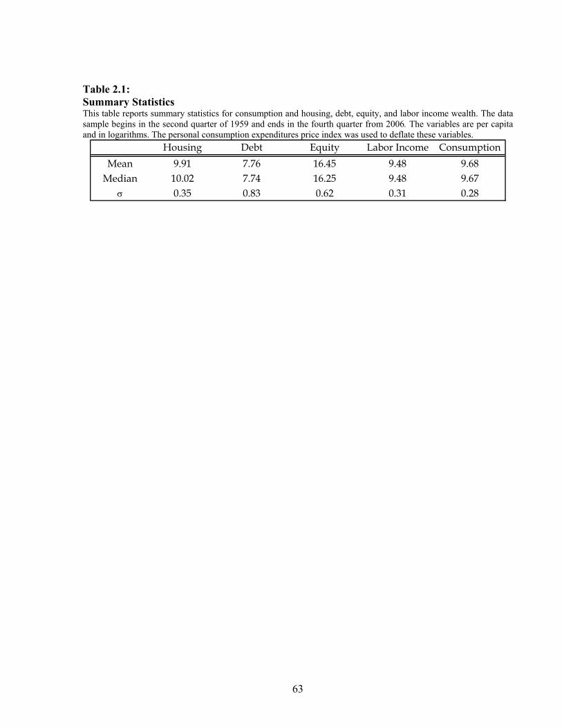
63

Table 2.1: Summary Statistics This table reports summary statistics for consumption and housing, debt, equity, and labor income wealth. The data sample begins in the second quarter of 1959 and ends in the fourth quarter from 2006. The variables are per capita and in logarithms. The personal consumption expenditures price index was used to deflate these variables.

Housing Debt Equity Labor Income ConsumptionMean 9.91 7.76 16.45 9.48 9.68

Median 10.02 7.74 16.25 9.48 9.67σ 0.35 0.83 0.62 0.31 0.28

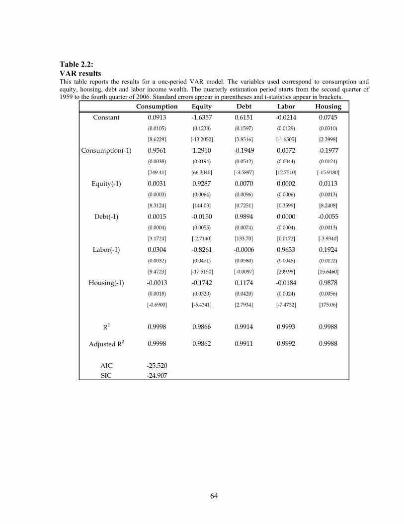
64

Table 2.2: VAR results This table reports the results for a one-period VAR model. The variables used correspond to consumption and equity, housing, debt and labor income wealth. The quarterly estimation period starts from the second quarter of 1959 to the fourth quarter of 2006. Standard errors appear in parentheses and t-statistics appear in brackets.

Consumption Equity Debt Labor HousingConstant 0.0913 -1.6357 0.6151 -0.0214 0.0745

(0.0105) (0.1238) (0.1597) (0.0129) (0.0310)

[8.6229] [-13.2050] [3.8516] [-1.6505] [2.3998]

Consumption(-1) 0.9561 1.2910 -0.1949 0.0572 -0.1977(0.0038) (0.0194) (0.0542) (0.0044) (0.0124)

[249.41] [66.3040] [-3.5897] [12.7510] [-15.9180]

Equity(-1) 0.0031 0.9287 0.0070 0.0002 0.0113(0.0003) (0.0064) (0.0096) (0.0006) (0.0013)

[8.3124] [144.03] [0.7251] [0.3599] [8.2408]

Debt(-1) 0.0015 -0.0150 0.9894 0.0000 -0.0055(0.0004) (0.0055) (0.0074) (0.0004) (0.0013)

[3.1724] [-2.7140] [133.70] [0.0172] [-3.9340]

Labor(-1) 0.0304 -0.8261 -0.0006 0.9633 0.1924(0.0032) (0.0471) (0.0580) (0.0045) (0.0122)

[9.4723] [-17.5150] [-0.0097] [209.98] [15.6460]

Housing(-1) -0.0013 -0.1742 0.1174 -0.0184 0.9878(0.0018) (0.0320) (0.0420) (0.0024) (0.0056)

[-0.6900] [-5.4341] [2.7934] [-7.4732] [175.06]

R2 0.9998 0.9866 0.9914 0.9993 0.9988

Adjusted R2 0.9998 0.9862 0.9911 0.9992 0.9988

AIC -25.520SIC -24.907

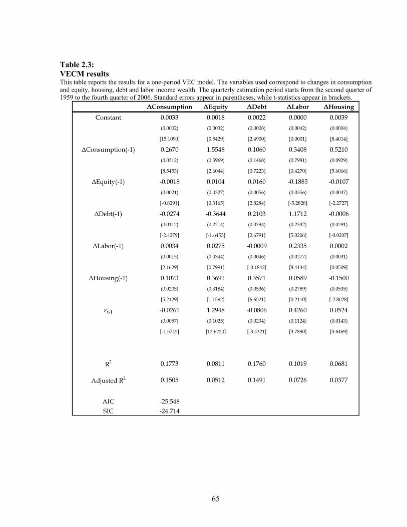
65

Table 2.3: VECM results This table reports the results for a one-period VEC model. The variables used correspond to changes in consumption and equity, housing, debt and labor income wealth. The quarterly estimation period starts from the second quarter of 1959 to the fourth quarter of 2006. Standard errors appear in parentheses, while t-statistics appear in brackets.

ΔConsumption ΔEquity ΔDebt ΔLabor ΔHousingConstant 0.0033 0.0018 0.0022 0.0000 0.0039

(0.0002) (0.0032) (0.0008) (0.0042) (0.0004)

[15.1090] [0.5429] [2.4900] [0.0001] [8.4014]

ΔConsumption(-1) 0.2670 1.5548 0.1060 0.3408 0.5210(0.0312) (0.5969) (0.1468) (0.7981) (0.0929)

[8.5453] [2.6044] [0.7223] [0.4270] [5.6066]

ΔEquity(-1) -0.0018 0.0104 0.0160 -0.1885 -0.0107(0.0021) (0.0327) (0.0056) (0.0356) (0.0047)

[-0.8291] [0.3165] [2.8284] [-5.2828] [-2.2727]

ΔDebt(-1) -0.0274 -0.3644 0.2103 1.1712 -0.0006(0.0112) (0.2214) (0.0784) (0.2332) (0.0291)

[-2.4279] [-1.6453] [2.6791] [5.0206] [-0.0207]

ΔLabor(-1) 0.0034 0.0275 -0.0009 0.2335 0.0002(0.0015) (0.0344) (0.0046) (0.0277) (0.0031)

[2.1629] [0.7991] [-0.1842] [8.4134] [0.0509]

ΔHousing(-1) 0.1073 0.3691 0.3571 0.0589 -0.1500(0.0205) (0.3184) (0.0536) (0.2789) (0.0535)

[5.2129] [1.1592] [6.6521] [0.2110] [-2.8028]

εt-1 -0.0261 1.2948 -0.0806 0.4260 0.0524(0.0057) (0.1025) (0.0234) (0.1124) (0.0143)

[-4.5745] [12.6220] [-3.4321] [3.7880] [3.6469]

R2 0.1773 0.0811 0.1760 0.1019 0.0681

Adjusted R2 0.1505 0.0512 0.1491 0.0726 0.0377

AIC -25.548SIC -24.714

66

Table 2.4: In-Sample Forecast Regressions The table reports estimates from OLS regressions of stock returns on lagged variables. Regressions use quarterly data from the second quarter of 1959 to the fourth quarter from 2006. I use the CRSP VW to calculate real returns as dependent variables. As the main predictor variable, I use the changes in expectations of consumption to wealth ratio

(u-ccwt) plus the changes in expectations of the discounted future consumption growth ( ∑∞

=+− Δ−

11)(

iit

itt cEE ρ ). For

means of comparison, I also use Lettau and Ludvigson (2001a) measure cayt, cedyt (consumption to wealth ratio measurement that excludes housing), a lag of the endogenous variable, lag, the log dividend to earnings ratio and to price ratio, dt.-et and dt.-pt, and the short term interest rates, shortt. All predictors are at time t. The personal consumption expenditures price index was used to calculate real returns. Significant coefficients at the 5 percent level from a two-tail test are bolded.

# Constant lag cay t cedy t d t - p t d t - e t short t u-ccw t (E t -E t-1 )

1 0.018 0.028 0.00(3.016) (0.385)

2 0.019 1.498 0.05(3.291) (3.347)

3 0.030 0.967 0.04(5.516) (2.858)

4 0.001 0.051 0.02(0.092) (1.378)

5 0.011 0.006 0.00(0.453) (0.352)

6 0.019 -0.013 0.03(3.314) (-2.227)

7 0.019 1.482 -5.307 0.03(8.966) (4.887) (-5.081)

Real Returns; 2Q 1959 - 4Q 2006

2R∑∞

= +Δ1i it

i cρ

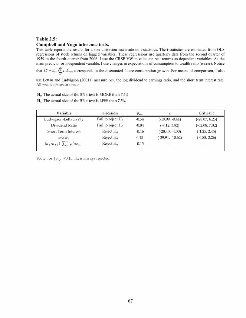
67

Table 2.5: Campbell and Yogo inference tests. This table reports the results for a size distortion test made on t-statistics. The t-statistics are estimated from OLS regressions of stock returns on lagged variables. These regressions use quarterly data from the second quarter of 1959 to the fourth quarter from 2006. I use the CRSP VW to calculate real returns as dependent variables. As the main predictor or independent variable, I use changes in expectations of consumption to wealth ratio (u-ccw). Notice

that ∑∞

=+− Δ−

11)(

iit

itt cEE ρ corresponds to the discounted future consumption growth. For means of comparison, I also

use Lettau and Ludvigson (2001a) measure cay, the log dividend to earnings ratio, and the short term interest rate. All predictors are at time t. H0: The actual size of the 5% t-test is MORE than 7.5%H1: The actual size of the 5% t-test is LESS than 7.5%

Variable Decision ρu,ε c Critical cLudvigson-Lettau's cay Fail to reject H0 -0.54 (-19.99, -0.41) (-28.07, 6.25)

Dividend Ratio Fail to reject H0 -0.84 (-7.12, 3.82) (-62.08, 7.82)Short Term Interest Reject H0 -0.16 (-28.43, -4.30) (-1.25, 2.45)

u-ccw t Reject H0 0.15 (-39.94, -10.62) (-0.88, 2.26) (E t -E t-1 ) Reject H0 -0.13 - -

Note: for |ρu,ε|<0.15, H0 is always rejected

∑∞

= +Δ1i it

i cρ

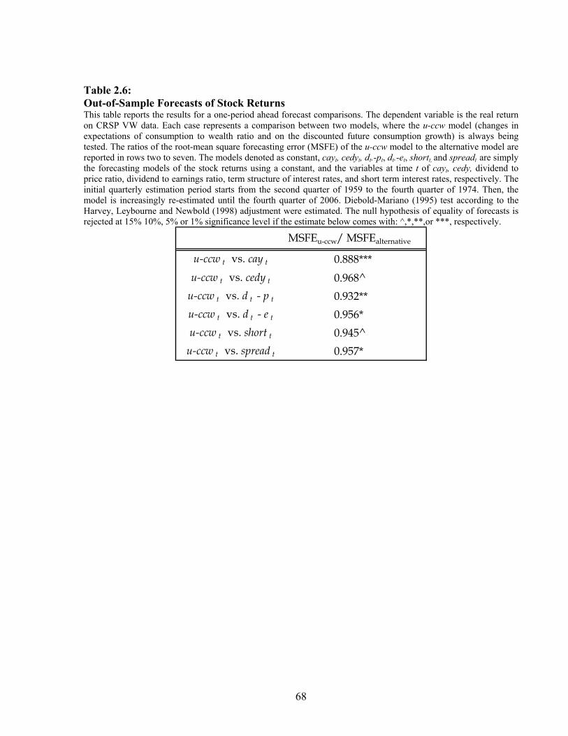
68

Table 2.6: Out-of-Sample Forecasts of Stock Returns This table reports the results for a one-period ahead forecast comparisons. The dependent variable is the real return on CRSP VW data. Each case represents a comparison between two models, where the u-ccw model (changes in expectations of consumption to wealth ratio and on the discounted future consumption growth) is always being tested. The ratios of the root-mean square forecasting error (MSFE) of the u-ccw model to the alternative model are reported in rows two to seven. The models denoted as constant, cayt, cedyt, dt.-pt, dt.-et, shortt, and spreadt are simply the forecasting models of the stock returns using a constant, and the variables at time t of cayt, cedy, dividend to price ratio, dividend to earnings ratio, term structure of interest rates, and short term interest rates, respectively. The initial quarterly estimation period starts from the second quarter of 1959 to the fourth quarter of 1974. Then, the model is increasingly re-estimated until the fourth quarter of 2006. Diebold-Mariano (1995) test according to the Harvey, Leybourne and Newbold (1998) adjustment were estimated. The null hypothesis of equality of forecasts is rejected at 15% 10%, 5% or 1% significance level if the estimate below comes with: ^,*,**,or ***, respectively.

MSFEu-ccw/ MSFEalternative

u-ccw t vs. cay t 0.888***u-ccw t vs. cedy t 0.968^

u-ccw t vs. d t - p t 0.932**u-ccw t vs. d t - e t 0.956*u-ccw t vs. short t 0.945^

u-ccw t vs. spread t 0.957*

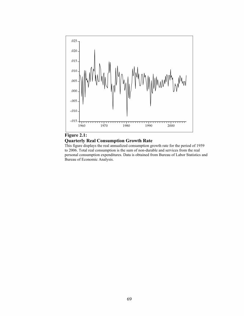
69

-.015

-.010

-.005

.000

.005

.010

.015

.020

.025

1960 1970 1980 1990 2000

Figure 2.1: Quarterly Real Consumption Growth Rate This figure displays the real annualized consumption growth rate for the period of 1959 to 2006. Total real consumption is the sum of non-durable and services from the real personal consumption expenditures. Data is obtained from Bureau of Labor Statistics and Bureau of Economic Analysis.

70

Figure 2.2: Welch and Goyal performance test The graph plots: elealternativ

ti

tmeanprevailing

ti SESESSENet mod1975

−= ∑ =, where tSE is the square out-of-sample

prediction errors in time t, and i goes from the first quarter of 1975 to the fourth quarter of 2006. The “prevailing mean” SEt is obtained when the prevailing up-to-date CRSP returns’ average is used to forecast the t+1 return. The “alternative model” SE’s are obtained from rolling regressions with either u-ccw, cay, dividend ratio or short term interest rate as the (sole) predictor of time t+1 CRSP returns. For a quarter in which the slope is positive the alternative model predicted better than the unconditional average out-of-sample.

1980

1985

1990

1995

2000

2005

-0.015-0.0

1

-0.0050

0.0050.01

0.0150.02

0.025

U-CCW

Net SSE

Years

1980

1985

1990

1995

2000

2005

-0.16

-0.14

-0.12

-0.1

-0.08

-0.06

-0.04

-0.020

CAY

Net SSE

Years

1980

1985

1990

1995

2000

2005

-0.08

-0.06

-0.04

-0.020

0.02

Divide

nd Ra

tio

Net SSE

Years

1980

1985

1990

1995

2000

2005

-0.06

-0.05

-0.04

-0.03

-0.02

-0.010

0.01

0.02

Short

Intere

st Rate

Net SSE

Years

71

CHAPTER 3: WILL PULLING OUT THE RUG HELP? – UNCERTAINTY

ABOUT FANNIE AND FREDDIE’S FEDERAL GUARANTEE AND

THE COST OF THE SUBSIDY

3.1. Introduction

Fannie Mae and Freddie Mac (F&F) are financial intermediaries created by the Congress

of the United States to foster liquidity in the housing loan market, and to fund loans to certain

groups of borrowers such as homeowners, farmers and students (Appendix 3.A provides

background information about the activities of these entities). These two Government Sponsored

Enterprises earn a fee when they purchase mortgage loans from diverse financial institutions, and

then pool and resell them to investors as financial securities. In addition to the fee business, F&F

often hold onto some of their securitized loans to earn interest income. Table 3.1 provides the

annual earnings of Freddie Mac from the two sources of business (fee and investment portfolio

interest income) for the period 1990 to 2006.

The securitized assets in the investment portfolio held by F&F are funded for the most

part by borrowings via sale of debt. It is widely believed by the lenders of funds to F&F (debt

holders) that they will be fully reimbursed by the government were F&F to experience distress

and default on their obligations. This belief that debt holders are not likely to face losses in the

event of bankruptcy has lead to low bond spreads, increased liquidity in these assets and a

corresponding growth in the size of the F&F debt market. In 2005, the face value of outstanding

debt of F&F (Fannie and Freddie) totaled more than $2 trillion (see Table 3.2). However, the

72

assumption of a federal guarantee of F&F debt, that spurred growth in the F&F debt market, has

been recently called to question. In a hearing15 Alan Greenspan remarked:

“there is a perception that debt holders are guaranteed by the full faith and the credit of the United States government, despite the fact that the debentures which they bought and literally say, as required by the law, that this instrument is not backed by the full faith and credit.”

Subsequently, the Former Secretary of the Treasury (John Snow) made the following comments,

when asked whether he would use his discretionary ability to bail out F&F debt holders in the

event of default16:

“Some commentators believe that this credit availability reinforces the perception that the Federal government backs the debt obligations of the Enterprises. This perception is false.”

Such pronouncements by regulators and politicians are motivated in part by the potential cost

that could be borne by taxpayers were these entities to default.17 This uncertainty about whether

the government will bail out debt holders raises several questions, important both for policy

makers as well as for the claimholders (i.e. for debt and equity holders of F&F), and are not fully

addressed in the literature:

o First, how and to what extent does the uncertainty about the Federal Guarantee impact F&F equity prices and debt prices?

o Second, will the government stance on voicing uncertainty about the guarantee help reduce the cost of this subsidy to taxpayers?

In this paper we answer the two questions posed by providing a simple model for the value of

F&F where there is uncertainty about the government guarantee. A Federal Guarantee of debt,

15 See discussion in Housing and Urban Affairs Committee hearing (July 21, 2005) chaired by Senator Richard Shelby. 16 See testimony of Secretary John Snow before the U.S. House Financial Services Committee Proposals for Housing F&F Reform on April 13, 2005. 17 Seiler (2003) documents such instances when there have been public pronouncements about the likelihood of government support, were they to default. The author finds that these pronouncements impact debt and equity prices negatively, as financial market participants reassess the risk of these assets.

73

and any uncertainty about it, comes into play only if the firm experiences financial distress.

Thus, it is important to characterize the probability that F&F may experience distress and default.

From the modeling perspective, our main contribution is that we determine this probability using

observable variables of the firm and then evaluate how the uncertainty impacts this probability of

distress.

As noted earlier, F&F engage in two lines of business- First, they earn a fee on the

mortgages they buy and then resell to investors, after pooling and securitizing the loans. This

constitutes their core fee based business. Second, F&F hold mortgage backed security (MBS)

portfolios to accrue the spread (difference) between their low cost of capital and the higher yield

of the mortgage portfolio. Table 3.1 shows that fee income for Freddie Mac was 1.8 billion,

before costs, in 2006. The fee income has increased steadily and the growth rate has not varied

substantially (standard deviation of earnings growth is 10%). Also, interest income from the

portfolio holdings was around 43 billion in 2006 but its earnings growth has varied considerably

over the data period (standard deviation of earnings growth is around 38%).

To assess the impact of the guarantee we first separate out the firm into these two parts –

the value of the firm due to the earnings in the fee business and the value due to the earnings of

interest income (both of these income flows are observable). The firm value of F&F, if there

were no debt financing, is simply equal to the present value of the cash flows from the two

sources (in the same vein as Passmore (2005)). There is obviously no role for the government

guarantee if the firm has not borrowed any money (when there is no debt).

F&F borrow to finance their business because it affords them certain advantages. As

long as these advantages outweigh the costs, F&F are inclined to continue borrowing to run their

74

business. The value of the firms when F&F borrow to finance their business is equal to the sum

of -

(1) the value of the business without borrowing plus (2) the present value of the tax savings and the increased earnings attributable to debt

financing when there is a guarantee, and minus any costs that are result of the debt financing.

In terms of the advantages of using debt in the presence of a guarantee, financing via debt adds

value for three reasons. First, interest payments are tax deductible and this makes the financing

cheaper relative to equity financing. Even though F&F are exempt of state and local corporate

income taxes and the tax advantage of leverage is lower than that for regular corporations, it still

accounts for substantive savings. Second, the federal guarantee makes this avenue a cheaper

source of long-term funds for F&F because debt holders demand lower coupons since they are

likely to face a lower cost in case the firm was to go bankrupt. Other one-time costs incurred in

the issuance of debt are lower in contrast to alternate forms of borrowing.18 This cheap debt

financing allows them to increase the earnings spread on their mortgage portfolios relative to the

interest cost of financing. Third, other firms that enter into contracts with F&F to help hedge or

protect the mortgage security holdings from interest rate changes provide better terms on such

contracts (discussed in more detail later).

In contrast to the benefits of debt, F&F may want to limit the issuance of debt for a

number of reasons. Increases in the amount of debt will increase the possibility that the firm

will go bankrupt when it is unable to make these promised interest payments. As F&F hold more

investment securities in their portfolio that are financed via debt, the increased risks (credit risk,

18 Debt issuance to finance the assets of the firm is beneficial for a number of other reasons. F&F debt is exempt from registration with the Securities and Exchange Commission, thus reducing floatation costs. These bonds are treated as quasi-government securities by most investors because investors perceive these securities to be backed by the government. Some banks are allowed to make unlimited investments in F&F debt securities, and F&F securities are eligible as collateral for public deposits as well as for Treasury tax and loan accounts, which makes them attractive to investors. All these benefits result in a lower funding cost for F&F.

75

prepayment risk and interest rate risk) may make the value of these earnings more volatile.

Thus, with more debt on the books, the probability that F&F will not be able to meet their

obligations increase, and the tax benefits may not be commensurate with the costs. In sum, the

benefit of debt financing are tax benefits, low costs of borrowing and better terms on borrowing

and hedging of their assets. The cost is that there could be adverse movements in the value of

the portfolio and cause the firm to face financial distress.

Uncertainty about the guarantee impacts the firm’s earnings via two channels. A first

avenue is the increased interest cost on any new debt that is sold. Now, the uncertainty impacts

the firm value through its impact on the expected losses in bankruptcy when the F&F are not

able to pay their interest obligations (bankruptcy costs). When there are larger losses in

bankruptcy, the debt holders must be compensated by a larger interest payment. Debt holders

demand a higher coupon and the profitability of the firm’s asset portfolio will decrease.

However the magnitude of this effect is small, given that in the current scenario, F&F values are

high enough to make the overall likelihood of bankruptcy quite low. It is important to note that

existing borrowings will be subject to the new costs only when existing debt is refunded and new

debt is sold. Many of the borrowings are longer term, and the new risk will be re-priced only

when any new bonds are sold. In addition, F&F debt enjoys extra liquidity because market

participants perceive it to be a convenient short-term place to park their funds. As a result the

low yield in part reflects the extra liquidity of these bonds. Increased uncertainty of the

guarantee may add to the coupon demanded by lenders because this liquidity benefit is also

reduced.

A second, and more important, channel by which the increased uncertainty impacts F&F

immediately is that it reduces the earnings on its MBS portfolio. As we had noted, F&F enter

76

into contracts on a continual basis with other financial institutions to hedge their portfolio against

changes in interest rates caused by macroeconomic shocks. Because F&F are constantly entering

into new contracts, these contracts allow for re-evaluation of the risk at short intervals as

compared to bankruptcy costs on debt which are revalued only when new debt is sold. The costs

of hedging the asset portfolio from interest rate shocks will therefore increase right away as a

result of this uncertainty. This happens because an increase in the uncertainty about the federal

guarantee is likely to increase the capital (margin) required by banks and financial institutions

that enter into hedging arrangements with F&F (see for example Cooper and Mello (1992)).

Risk managers at these institutions are likely to reassess the losses that would be incurred in case

of default within a short time frame. This is somewhat related the liquidity advantage of debt

because sellers of these hedging contracts use F&F debt to protect their overall risk, and their

ability to do so is linked to liquidity of the debt. The resultant increases in margin would

consequently reduce the earnings of the mortgage portfolio and the overall value of the firm

substantially in light of the fact that over 80% of the firms’ earnings are derived from the

investment portfolio, and hedging of the portfolio is an important aspect of its activities. An

increase in uncertainty about the guarantee that increases the costs of hedging by 10 basis points

can decrease the firm value by 15%.19 Hence small changes in the uncertainty of the guarantee

are likely to dramatically impact the firm value via a decrease in returns on the investment

portfolio. This aspect of feedback of the credit risk of a firm on its earnings is more pronounced

because the capitalized earnings on the security portfolio contribute to a large proportion of the

firm value.

To analyze the feedback of the uncertainty on the value of F&F, our model takes as

inputs the cash flows from the two lines of business, the fee business and the investment 19 These numbers are approximated from F&F balance sheet information.

77

portfolio business described above. In this second line of business, we include the cash flows

that are a result of the fact that the security holdings are funded in large part by borrowings or

debt that has an implicit guarantee. We obtain closed formed solutions for the value of the firm,

its debt and its equity, and relate these values to firm risk, taxes, bankruptcy costs, among other

parameters20. Our main contribution is that we incorporate the probability that the government

may let F&F fail in case one of them files for bankruptcy. This allows us to focus on the two

questions posed: the impact of the uncertainty on the value of debt, equity and the cost of the

subsidy. Despite the simplicity of the model, it is useful from a practical perspective because of

the limited inputs required.

Researchers argue that the “implicit subsidy” that flows from the guarantee by the

federal government produces a surplus of billions of dollars and is directed to F&F shareholders

(Lehnert, Passmore and Sherlund (2006))21. We analytically determine the value of this implicit

subsidy and the impact on the subsidy when there is some uncertainty about whether the

government would step in, were F&F to default. Our article can be regarded as an extension of

the reduced form approach employed by Passmore (2005). While Passmore (2005) directly

estimates the value of the implicit guarantee using a discounted cash flow approach, we allow the

cash flows to be contingent on the value of the firm. We are able to estimate the funding

advantage of F&F, the extent to which F&F would reduce their relative holding of mortgage

backed securities in the absence of a government guarantee as well as the extent to which

shareholders retain the value of the funding advantage. In related work, Lucas and McDonald 20 The quantitative approach to modeling a firm’s assets and liabilities was pioneered by Black and Scholes (1973), Merton (1974) and extended by Black and Cox (1976), and others. 21 A clearer example how the implicit government backing works is illustrated with Fannie’s problem of insolvency in the 1980s. In the beginning of such decade, the interest rates peaked and earnings on Fannie’s portfolios weren’t high enough to meet its liabilities. The main reason why Fannie made it through was because banks kept lending it money—based on the idea that the government stood behind Fannie. Thus, if everyone thinks that the government will not let F&Fs fail, the likelihood that these companies will not be subject to market discipline will rise, further generating a moral hazard problem.

78

(2006) specify the dynamics of the firm assets and liabilities to compute the value of the implicit

subsidy (see discussion in Lehnert and Passmore (2006)). This article also related to their

general approach but our model is more appropriately characterized as a variant of the models of

capital structure presented in the corporate finance literature. This model is easily implemented

and has the advantage of closed form solutions.

The value of the implicit subsidy obtained in our setting, $121 billion, is similar to that

obtained by Passmore (2005) even though it is substantially higher than that obtained in some

other studies. Also, the valuation of the implicit subsidy is directly related to the formulation

obtained at the outset by Passmore (2005). We determine the extent to which uncertainty about

the subsidy may affect the cost of the subsidy to the government. Policy makers argue that the

government should clarify the potential misperception about the subsidy to the F&F, and thus

stem their growth rates and reduce the potential cost to the tax payer. Interestingly, an increase

in the likelihood of revocation can reduce firm value dramatically that may in turn double the

expected costs to tax payers. A more realistic avenue to reduce this cost to taxpayers is to cap

the size of the investment portfolio. This is consistent with some recent statements by the

Federal Reserve Chairman Ben Bernanke (discussed later in Section 3.4).

Our model requires five basic inputs, each of which are observable- the earnings flow of

the fee business, the earnings flow of the portfolio business, the interest cost of debt, its spread

over a comparable treasury bond, and the earnings volatility of the business. The model is

consequently transparent and easily understood. From an economic and intuitive standpoint, it

provides a convenient starting point for the questions posed.

The article is organized as follows. Section 3.2 describes our model. Closed form

solutions are derived for debt, equity and firm values when there is uncertainty about the extent

79

of the federal guarantee. Section 3.3 analyzes the impact of the uncertainty about the implicit

guarantee on firm value and debt and equity prices. Section 3.4 calculates the value of the

implicit subsidy and discusses extensions of the model and Section 3.5 concludes.

3.2. The model

Our objective is to analyze the impact of uncertainty about the federal guarantee on F&F

debt and equity prices. In doing so, we elicit the impact of uncertainty about the guarantee on

the expected cost of the subsidy.

We start by defining the value of F&F earnings when the firm uses no debt to finance the

firm and consequently there is no role of the guarantee. Following the finance literature, the

present value of the earnings flow gives the value of the firm. Using this as a starting point, we

then analyze the change in the earnings and firm value when debt is used to finance the firm, and

there is uncertainty about the guarantee. Use of debt to finance the firm changes the value of the

firm because the firm benefits from tax deductions. At the same time, it is important to

determine the cost of debt- the probability that the firm may not be able to meet its obligations

and file for bankruptcy. This is especially important in our setting because the purpose of this

paper is to evaluate the cost of the federal guarantee that comes into play only if the firm is

unable to meet its obligations. We obtain the value of F&F debt, the value of the firm and the

value of equity (the residual claim on the assets of a firm).22 Later in Section 3.4 we use the

results obtained to compute the cost of the subsidy to taxpayers as well as its benefit to equity

holders.

22This approach is commonly employed in the finance literature (e.g., Leland (1994))

80

3.2.1 Value of the business when there is no debt

Recall that the value of a business is simply the expected present value of its earnings

where the present value is taken at the appropriate risk adjusted rate. Accordingly, we first

characterize the earnings of the firm when there is no role for uncertainty in the guarantee, i.e.,

when the firm has no debt on its books. Fannie Mae and Freddie Mac operate two independent

business lines: (1) a fee based business associated with securitizing mortgages that are sold off

to other investors, and (2) a portfolio investment business that involves holding various mortgage

backed securities.

Fee based business

From Table 3.1, in the year 2006, Freddie Mac earned approximately $1.8 billion in

commissions and fees and incurred administrative costs (average of 22%), tax and related costs

(average of 23%) to give net earnings of approximately $1 billion. These earnings are uncertain

and vary through time. Equation (1), that defines these earnings changes below, merely says

that the earnings 1δ grow at a certain rate each year ( 1μ ) but experience shocks each period that

are drawn from a normal distribution with volatility 1σ . This equation is commonly referred to

as the process governing the earnings changes (for risk-neutral investors):

1111

1 dzdtd

σμδδ

+= (1)

where 1μ is a constant and refers to the growth rate in the fee business, 1σ is that instantaneous

volatility of the earnings, dt is the increment in time, 1dz is the instantaneous shock to earnings

(increment of a Brownian Motion). From Table 3.1, the earnings for Freddie Mac have an

annualized standard deviation of around 10%. Then, the value of the business is equal to the

81

present value of the cash flows it generates: 1

11 μ

δ−

=r

V . Thus, when the earnings are $1 Billion

and r=6% and with a growth rate of 1μ =2%, the value of this business works out to

25$02.006.0

11 =

−=V billion. 1V is also referred to as the unlevered value of this line of

business because it assumes no consideration about debt financing.

Portfolio business

In addition to this first line of business, a second line of business generates returns by

holding a portfolio of securities on its books. The firm is able to generate a revenue stream equal

to a proportion of the amount of security inventory on its books. In 2006, Freddie Mac earned

approximately 43 billion dollars on its investment portfolio of nearly 900 billion. Then, in the

absence of tax benefits of debt (because we are first considering an unlevered firm) and

including hedging and administrative costs, the net earnings are around 23 billion dollars a year.

The earnings of this business, per dollar of securities held (around 23/900 or approximately 2.5%

in our case), are governed by the following process under the risk neutral measure:

2222

2 dzdtdσμ

δδ

+= (2)

where 2μ is a constant, 2σ is that instantaneous volatility of the earnings and 2dz is the

instantaneous shock to earnings. Then the corresponding value of this part of the business is

equal to 2

22 μ

δ−

=rFV where F is the face value of securities held. When r=6% and with a

growth rate of 2μ =2%, the value of this business works out to 02.06.

23−

=$575 billion.

82

It is important to note that the earnings of the firm from this second line of business

depend on its creditworthiness. If the government does not support debt holders, financial

institutions that trade with F&F would impose additional margin and other costs when they enter

into long term contracts with F&F. Hence 2δ (earnings per dollar of securities held) of F&F

would be lower if the costs of hedging and managing the mortgage portfolio were to increase.

Empirical estimates suggest that the total funding advantage of F&F is approximately 40 to 60

basis points (e.g., Passmore (2005)). Removing the federal guarantee would increase the

hedging costs to this extent so as to incorporate the increased risks borne by corporations that

enter into longer term deals (e.g., swaps) with F&F. Later, we assume that the earnings on the

mortgage portfolio are equal to 2δ minus a penalty if there is uncertainty about the guarantee.

Our assumption is that the earnings are adjusted for the probability (p) that the government will

not pay up: p005.02 −= δδ where 025.0=δ in this case. In other words, when the

government revokes the guarantee, earnings would decline by a maximum of 50 basis points or

0.5% per unit of securities held.

The total value of both businesses

The total value (in the absence of debt) of F&F is then given by the sum of the values of the two

business lines. Here the value of the firm at time zero is denoted by:

21 VVV += . (3)

In our case this total firm value works out to 25 billion + 575 billion for a total of $600 billion.

As noted, the returns to the fee business and portfolio of securities are time varying and

uncertain. Clearly the investment portfolio will bear substantial interest rate and credit risk, even

if some of the risks are hedged by a F&F. Now, the overall growth in total firm value (V) is

83

contributed by earnings from both lines of business. Correspondingly, the overall risk of the

two lines of business is dependent on the proportion of earnings from each business and the

correlation between the businesses. The correlation is nearly zero for the sample period and so

the blended risk of the two businesses is approximated as 22

221

22 )1( σσσ yy +−= where y is the

proportional value of each business, and is fixed. If y=0.8, the overall risk of the portfolio is

around 30% per year. This risk gives the instantaneous volatility of the firm’s assets and

captures all risks that may cause the value of the business to fluctuate. Thus overall volatility is

a blend of the core fee business and the interest rate and liquidity risk of the asset portfolio,

among other sources of risk.

3.2.2 Uncertainty in the guarantee and the role of debt

In the previous section, we outlined the value of the business when there is no debt.

Suppose now that the F&F borrow to finance some of their assets. While debt financing adds

value because of tax deductibility, there is a possibility that the firm is unable to meet its

obligations of interest payments and consequently experience distress. To evaluate the

probability of such an occurrence, we first assume that the value of the firm at which this occurs

is exogenous (we discuss its computation later). Suppose the firm value and its earnings evolve

through time unless the firm value declines and reaches a value BV when it is unable to pay its

coupons on the debt and is in financial distress (see Figure 3.2).

When the firm is in financial distress, the firm is handed over to debt holders and the

residual value is distributed amongst them. Let α−1 , where 0<α <1, be the fraction of the firm

value, BV , that is lost to bankruptcy costs in case the government does not guarantee the

liabilities. For example, if α−1 =0.5, then half of the value of the assets is lost. This leaves debt

84

holders with the amount α VB, and equity holders with nothing. These losses may in part be

direct legal costs, loss of human capital and other such costs.

Additionally, let *α , where 0< *α <1, to be the amount of firm value, BV , recovered in

case of default when government backs their debt, while *1 α− is the proportion lost to

bankruptcy costs incurred in this scenario. We set the value of *α to be greater than the value

ofα . For example *α could be 0.98. Then, 98% of the firm value is recovered when the

government steps in to compensate the debt holders. In both instances F&F file for bankruptcy,

though it is expected that if government backs their debt, bondholders will recover a higher level

of firm value at that time.

Assumption: We assume that there is an exogenous probability p that the government will not cover the losses to debt holders. This parameter captures the uncertainty about the guarantee.

We first obtain the value of the firm and then derive the value of debt and equity in the

subsequent sections.

3.2.2.1 Value of F&F when the costs and benefits of debt are included

While the firm was valued at $600 billion in our earlier example, equity holders may be

able to save on taxes and enhance firm value by borrowing and deducting these interest costs

from earnings. We now value the F&F when the firm sells debt to finance its business and there

is uncertainty about the guarantee.

Consider debt sold at time zero by equity holders to fund the business that in turn requires

the firm to pay a coupon flow C to debt holders each period. As we had discussed in the

introduction, issuing debt can increase firm value due to tax deductibility of the interest

85

payments but it increases the potential bankruptcy costs. Bankruptcy costs will depend on the

probability that the government will not guarantee F&F debt if the firm faces financial distress.

If government fully backs F&F debt then the amount lost due to bankruptcy will be low. On the

other hand, if F&F have no guarantee at all from the government, then their bankruptcy costs can

reduce substantially the amount of firm value left for bondholders. The total value of the firm

therefore depends on the probability of government support in case of financial distress, as well

as on the level of asset at which default is triggered.

Remark 1: The value of the firm for F&F with uncertainty about the federal guarantee is given by the sum of the firm value without debt, the tax benefits of debt and minus the costs were the firm to go bankrupt:

( ) [ ] )1()1)(1()1( *00 wVppw

rCVVFV B −−−+−−+= αατ (4)

where ⎥⎥⎦

⎤

⎢⎢⎣

⎡⎥⎦

⎤⎢⎣

⎡−=

−x

BVV

w 01 , ⎥⎥

⎦

⎤

⎢⎢

⎣

⎡+⎟⎟

⎠

⎞⎜⎜⎝

⎛−+⎟⎟

⎠

⎞⎜⎜⎝

⎛−= 2

222

2 222

1 σσσσ

rrrx , 210 VVV += ,

1

11 μ

δ−

=r

V , 2

22 μ

δ−

=rFV , p005.02 −= δδ .

Proof. See Appendix 3.B.

The firm value in equation (4) is the value of the firm without considering tax benefits of debt

( 0V ) plus the tax benefits and minus the bankruptcy costs. In equation (5), the tax benefits equal

the tax savings conditional on not defaulting- wrCτ . Of these tax benefits, the first term

rCτ is

the present value of the tax benefits of debt and the second term w corresponds to the probability

that the firm will not go bankrupt and continues to receive these tax benefits. Correspondingly,

in equation (5), the bankruptcy costs are the present value of losses incurred in default times the

86

probability of defaulting: ( ) )1()1)(1()1( * wpp −−−+− αα . Here the loss in firm value is (1-

*α ) with a probability (1-p) when the government guarantee is valid. The loss is larger, (1-α ),

if the debt is not guaranteed. Also note that the earnings 2δ on the second line of business

equals a fixed amount minus a penalty that depends on the probability that the government will

not guarantee the debt ( p005.02 −= δδ ).

3.2.2.2. The Value of Debt and Equity of F&F

We now value F&F debt when the firm sells debt to finance its business and there is uncertainty

about the guarantee. Debt is sold at time zero by equity holders to fund the business, with the

following characteristics- infinite maturity and a constant coupon flow C to debt holders each

period. Then, the price of debt at time 0 is written as the sum of two components- the expected

present value of:

(a) coupon flows if the firm value remains above VB and does not experience distress (with probability w ),

(b) payouts to debt holders if the firm value crosses VB and goes bankrupt. (with probability 1-w ),

Remark 2: The value of debt for a F&F with uncertainty about the federal guarantee is given by

( ) [ ] )1()1( *0 wVppw

rCVD B −−++= αα (5)

where ⎥⎥⎦

⎤

⎢⎢⎣

⎡⎥⎦

⎤⎢⎣

⎡−=

−x

BVV

w 01 , ⎥⎥

⎦

⎤

⎢⎢

⎣

⎡+⎟⎟

⎠

⎞⎜⎜⎝

⎛−+⎟⎟

⎠

⎞⎜⎜⎝

⎛−= 2

222

2 222

1 σσσσ

rrrx , 210 VVV += ,

1

11 μ

δ−

=r

V , 2

22 μ

δ−

=rF

V , p005.02 −= δδ .

Proof. See Appendix 3.B.

87

In equation (5), the first term is the present value of coupons conditional on not going

bankrupt (probability of not doing bankrupt is w) and the second term is the present value of the

payments if the firm becomes bankrupt. Again, in the second term the debt holders receive the

payout *α with a probability (1-p) when the government guarantee is valid. The payout is

lower α if the debt is not guaranteed.

Note that the coupon C comprises the coupons on the debt raised to finance the mortgage

portfolio plus any additional debt raised to finance the core business of the firm. There are

several possibilities on how to specify when the firm chooses to file for bankruptcy (the barrier

BV ). Lucas and McDonald (2006) assume a level equal to 70% of the value of the liabilities as

the trigger point in some examples. If returns to the asset portfolio are negative, and equity

holders need to fund coupon payments to the debt holders, the endogenous bankruptcy barrier is

characterized by Goldstein, Ju and Leland (2001). In our setting, using base case numbers from

the balance sheet for 2006, the endogenous trigger works also works out to nearly 80% of the

market value of debt. The substantive implications of our results are largely unchanged for

alternate levels at which the firm is declared bankrupt. In subsequent examples we assume an

endogenous barrier even though other conditions could be imposed. Equity value is the total

value of the firm minus the value of the firm owned by debt holders:

)()()( 000 VDVFVE −= (6)

In the subsequent sections we discuss the implications of the model obtained above. Equation

(6) gives the value of equity as a function of firm value and the volatility of firm value, amongst

other variables. A common problem in the implementation of these models is that the volatility

of firm value is not observable. In this context, Lucas and McDonald (2006) calibrate their

model to observed volatility of equity values and other parameters for F&F. The authors obtain

88

the implied volatility of equity values of Fannie Mae from option prices, and find that these

values vary between 16.7 percent and 60 percent over the year 2004. In our setting, the value of

the unlevered assets can also be gleaned by using the earnings flows of the firm.

For our model, we use our base case numbers with earnings of the first line of business

equal to 11 =δ , 025.2 =δ , 02.01 =μ , 02.02 =μ , %6=r , F=900, the value of the first line of

business works out to $25 billion and the second business is worth $575 billion (from equations

(1) to (3)). We fix the volatility of the first business at 10%, the volatility of asset values for the

second line of business at 38%, computed using numbers in Table 3.1. The bankruptcy trigger is

endogenous and the interest cost is C=37 billion, obtained from the data for 2006.

3.3. Impact of uncertainty about the federal guarantee

Our first objective is to analyze the impact of uncertainty about the federal guarantee on

F&F firm value, debt and equity values. A convenient outcome of this section is that it provides

an estimate of the extent to which equity-holders of F&F gain by the federal subsidy. Section

3.4 computes the expected cost of the subsidy to taxpayers.

3.3.1 Firm value with an uncertain guarantee

There is an ongoing discussion about the extent to which the federal guarantee increases

the value of F&F. In our setting, the federal guarantee reduces the risk of losses to bond holders

( *α , the recovered amount, is larger). Therefore, the guarantee allows the firm to earn a spread

between the lower costs of debt financing, relative to the yields on mortgage backed securities.

The presence of a government guarantee for F&F reduces the cost of funds for F&F relative to

89

other similar risk businesses run by other corporations. The reduced bankruptcy costs allows the

firm to take on more debt and avail the tax benefits of debt.

Also, F&F are better able to manage and hedge their portfolio holdings because of the

reduced risk and increased liquidity of their debt. Therefore, F&F are able to accrue profits over

and above what the appropriate risk return tradeoff would warrant by increasing the earnings per

dollar of securities held ( 2δ ).

An increase in uncertainty about whether the government will guarantee the debt

increases expected bankruptcy costs, and consequently increases the cost of new borrowing and

thus reduces the value of the firm. A second effect of increasing the uncertainty about the

guarantee is that the cost of hedging and managing the investment portfolio may increase. This

impact feeds into the earnings per dollar ( 2δ ) of the mortgage portfolio held by the F&F.

Using equation (4), Figure 3.3 provides a graphical analysis of the value of the firm as a

function of p, the probability that the government will not pay bond holders at default. We set

the interest rate %6=r , volatility of asset values 1.01 =σ and 38.02 =σ . If this uncertainty

increases, 2δ (earnings per dollar of securities held) of F&F would be lower. We set the

fractional return as a linear function of the uncertainty p005.02 −= δδ , so that higher

uncertainty results in increased hedging costs by 50 basis points if the government withdraws its

guarantee. The recovery rates are set at 5.0=α and 98.0* =α .

Figure 3.3 shows that as the probability of no guarantee increases, the value of the firm

decreases. This occurs because of the dual avenues via which the uncertainty effects firm value-

the increased probability of going bankrupt as well as reduced earnings on the mortgage

portfolio. The decline in the value of the firm from increased bankruptcy costs is of a lesser

90

order. The more significant loss in firm value occurs because of a reduction in the value of the

firm from reduced spreads earned on the investment side of the business.

Remark 3: F&F firm value decreases with higher uncertainty about the guarantee because of an increase in bankruptcy costs as well as the reduced profits on its mortgage portfolios.

3.3.2 Debt values and uncertainty in the guarantee

The potential funding advantage of F&F allows the firm to raise debt financing at a lower

relative spread in comparison with other firms with similar risk. This funding advantage and its

impact on F&F spreads is analyzed by Ambrose and Warga (2002), and others. On the one hand

the F&F are able to raise more funds because of the funding advantage, while on the other hand

increased leverage may in turn increase spreads because of increased chance of going bankrupt.

Our objective is to understand the impact of the uncertainty about the federal guarantee on F&F

debt prices and spreads.

Figure 3.4 illustrates the value of debt as a function of the uncertainty in the federal

guarantee, when the initial value of the first line of business is set at base case numbers in

Section 3.2. The volatility of asset values are as in the preceding example and the fractional

return on the second line of business is given by p005.02 −= δδ . Note that as p increases, the

value of debt decreases. Again, an increase in the uncertainty about the federal guarantee

decreases the firm value, and consequently the debt value because of the increased likelihood of

going bankrupt. The top line in Figure 3.4 does not account for increased hedging costs of the

mortgage portfolio while the bottom line includes such costs. The margin earned on the

91

investment portfolio is lower when there is a larger possibility that there will be no bail out of the

debt holders.

Remark 4: F&F debt values decrease with uncertainty about the guarantee because of an increase in bankruptcy costs as well as the reduced profits on its mortgage portfolios.

The equation for bond prices also allows us to evaluate the spread of bond yields over

treasury bonds: ( ) .0

rVDCSpread −= We can therefore analyze the extent to which the funding

advantage translates into reduced spreads in comparison with similar risk entities that do not

have such a government guarantee. Using our base case numbers, this spread works out to

approximately 69 basis points, quite close to the estimates obtained by Passmore (2005) but

higher than those estimated in Nothaft, Pearce and Stevanovic (2002) and Ambrose and Warga

(2002).

How much do equity holders benefit?

Figure 3.5 provides a graphical depiction of equity values and debt values as a function of

the uncertainty. Equity values are equal to the value of the firm less the value of debt (from

equation 6). Equity values decrease in lock step when debt values decrease. This is so because a

decrease in firm value makes equity values lower as well (a common outcome often discussed in

the corporate finance literature). Again, the firm value declines because the earnings from the

mortgage portfolio impact the overall firm value.

It is important to estimate how the subsidy benefits existing equity holders. Suppose

there was no subsidy, the first line of business with earnings 11 =δ billion after taxes would be

92

the mainstay of the business and the firm value is around $25 billion. This business has a

historical volatility of revenue changes of %101 =σ per year. Now, if the equity holders lever

up the firm to large extent and when the firm is financed with debt, the optimal amount of debt is

around $20 billion and the value of equity is around $9 billion when the firm has an amount of

debt that maximizes the value of the firm. If we were to throw in a subsidy at this point, and the

firm was to increase its security holdings of MBSs to the extent observed in Freddie Mac, the

value of the firm would increase to $635 billion and the value of equity increases to $67 billion

(using equations (4) to (6)). Hence, the federal subsidy has allowed equity holders to increase

their stake by around $58 billion in this setting. Thus, a large portion of the subsidy that is

provided by the government accrues to equity holders (In section 3.4 later we compute the value

of the subsidy equal to $121 billion of which $58 billion goes to equity holders).

This set up also allows us to examine the extent to which F&F would hold mortgage

portfolios were they to be financed without a government guarantee. As noted by Passmore

(2005), if F&F were purely private, they would hold far fewer MBSs on their books. If F&F did

not have any funding advantage, the fee business would constitute the core business and any

securities held would be based on considerations such as diversification benefits of income or

simply a providing an interim parking place for these securities.

3.4 Uncertainty and cost of the subsidy

The value of the implicit subsidy to tax payers has been the focus of much research in the

academic literature (see for example CBO studies (2001), Hubbard (2004), Jaffee (2003), Lucas

and McDonald (2006), Naranjo and Toevs (2002), Passmore (2005), Stiglitz, Orsag and Orsag

(2002)). There are several problems encountered in the computation of this liability. In

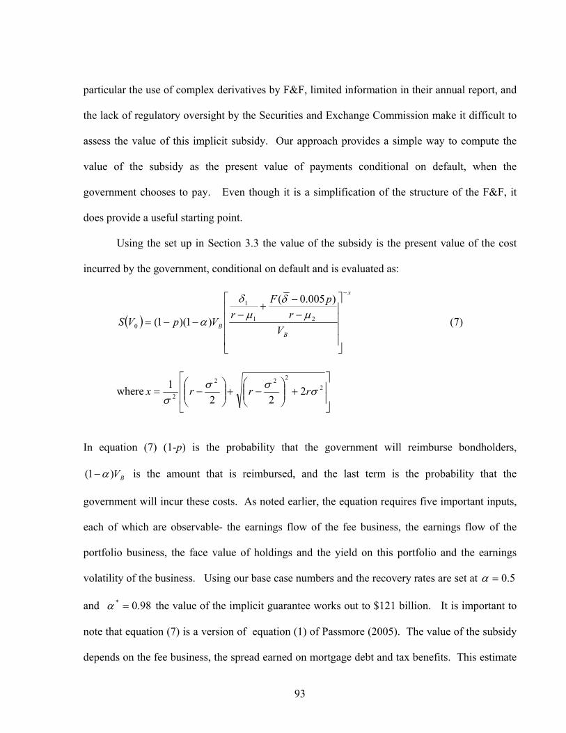
93

particular the use of complex derivatives by F&F, limited information in their annual report, and

the lack of regulatory oversight by the Securities and Exchange Commission make it difficult to

assess the value of this implicit subsidy. Our approach provides a simple way to compute the

value of the subsidy as the present value of payments conditional on default, when the

government chooses to pay. Even though it is a simplification of the structure of the F&F, it

does provide a useful starting point.

Using the set up in Section 3.3 the value of the subsidy is the present value of the cost

incurred by the government, conditional on default and is evaluated as:

( )

x

BB V

rpF

rVpVS

−

⎥⎥⎥⎥

⎦

⎤

⎢⎢⎢⎢

⎣

⎡−−

+−

−−= 21

1

0

)005.0(

)1)(1( μδ

μδ

α (7)

where⎥⎥

⎦

⎤

⎢⎢

⎣

⎡+⎟⎟

⎠

⎞⎜⎜⎝

⎛−+⎟⎟

⎠

⎞⎜⎜⎝

⎛−= 2

222

2 222

1 σσσσ

rrrx

In equation (7) (1-p) is the probability that the government will reimburse bondholders,

BV)1( α− is the amount that is reimbursed, and the last term is the probability that the

government will incur these costs. As noted earlier, the equation requires five important inputs,

each of which are observable- the earnings flow of the fee business, the earnings flow of the

portfolio business, the face value of holdings and the yield on this portfolio and the earnings

volatility of the business. Using our base case numbers and the recovery rates are set at 5.0=α

and 98.0* =α the value of the implicit guarantee works out to $121 billion. It is important to

note that equation (7) is a version of equation (1) of Passmore (2005). The value of the subsidy

depends on the fee business, the spread earned on mortgage debt and tax benefits. This estimate

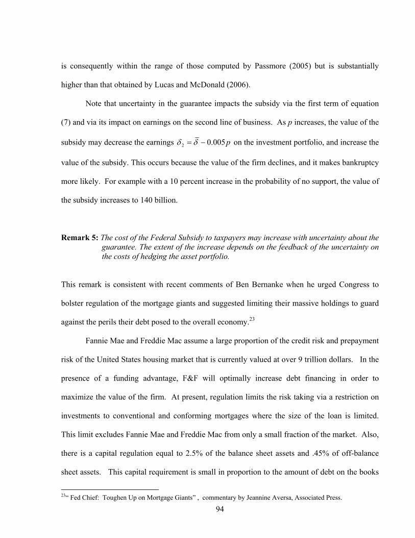
94

is consequently within the range of those computed by Passmore (2005) but is substantially

higher than that obtained by Lucas and McDonald (2006).

Note that uncertainty in the guarantee impacts the subsidy via the first term of equation

(7) and via its impact on earnings on the second line of business. As p increases, the value of the

subsidy may decrease the earnings p005.02 −= δδ on the investment portfolio, and increase the

value of the subsidy. This occurs because the value of the firm declines, and it makes bankruptcy

more likely. For example with a 10 percent increase in the probability of no support, the value of

the subsidy increases to 140 billion.

Remark 5: The cost of the Federal Subsidy to taxpayers may increase with uncertainty about the guarantee. The extent of the increase depends on the feedback of the uncertainty on the costs of hedging the asset portfolio.

This remark is consistent with recent comments of Ben Bernanke when he urged Congress to

bolster regulation of the mortgage giants and suggested limiting their massive holdings to guard

against the perils their debt posed to the overall economy.23

Fannie Mae and Freddie Mac assume a large proportion of the credit risk and prepayment

risk of the United States housing market that is currently valued at over 9 trillion dollars. In the

presence of a funding advantage, F&F will optimally increase debt financing in order to

maximize the value of the firm. At present, regulation limits the risk taking via a restriction on

investments to conventional and conforming mortgages where the size of the loan is limited.

This limit excludes Fannie Mae and Freddie Mac from only a small fraction of the market. Also,

there is a capital regulation equal to 2.5% of the balance sheet assets and .45% of off-balance

sheet assets. This capital requirement is small in proportion to the amount of debt on the books

23“ Fed Chief: Toughen Up on Mortgage Giants” , commentary by Jeannine Aversa, Associated Press.

95

and is unlikely to significantly impact the bankruptcy barrier or buffer the losses given default.

As pointed out, if the government were to take away this guarantee, the expected cost to the

government increases. A cap on the size of the portfolio will naturally increase the size of

equity relative to debt through time and consequently allow the government to reduce the extent

of the subsidy in an orderly manner.

In our setting, we model a firm where the extent of leverage is fixed. However, its is

possible that the proportion of the security holdings are adjusted downwards as the business

deteriorates. We assume that the volatility of the firm value and the face value of mortgage

holdings are constant even though the volatility of earnings of the firm and the holdings may

depend on the value of assets. A more generalized model can be obtained using the set up in

this paper, but may not add much to the analysis. One avenue to account for such effects is to

increase the overall value of the input to the volatility of the firm and make the face value of the

holdings a function of the firm value.

3.5. Conclusions

We analyze the implicit subsidy from the federal government via a model that

incorporates the ability of F&F to generate a revenue stream by selling mortgage backed

securities, as well as by holding these securities on its books via debt financing. The model can

be regarded as a reduced form cash flow approach that allows us to analyze the impact of

uncertainty about the implicit guarantee on F&F debt prices, bond spreads and equity values.

Regulators are concerned with providing a market based mechanism to control the

growth of the F&F portfolios. We show how a government pronouncement that increases the

uncertainty about the federal guarantee to a small extent can cause F&F values to decline by

96

large amounts. The increase in the likelihood that the government will not subsidize the F&F

may increase the expected costs of the subsidy to the government. Thus we argue that a cap on

the value of F&F investment portfolios is a more effective mechanism to reduce the growth rate

of these entities. Our model is easily applied to elicit the impact of the implicit subsidy on the

values of various financial claims of F&F. We address the extent to which existing equity

holders benefit from the subsidy and provide a convenient framework to address related policy

issues.

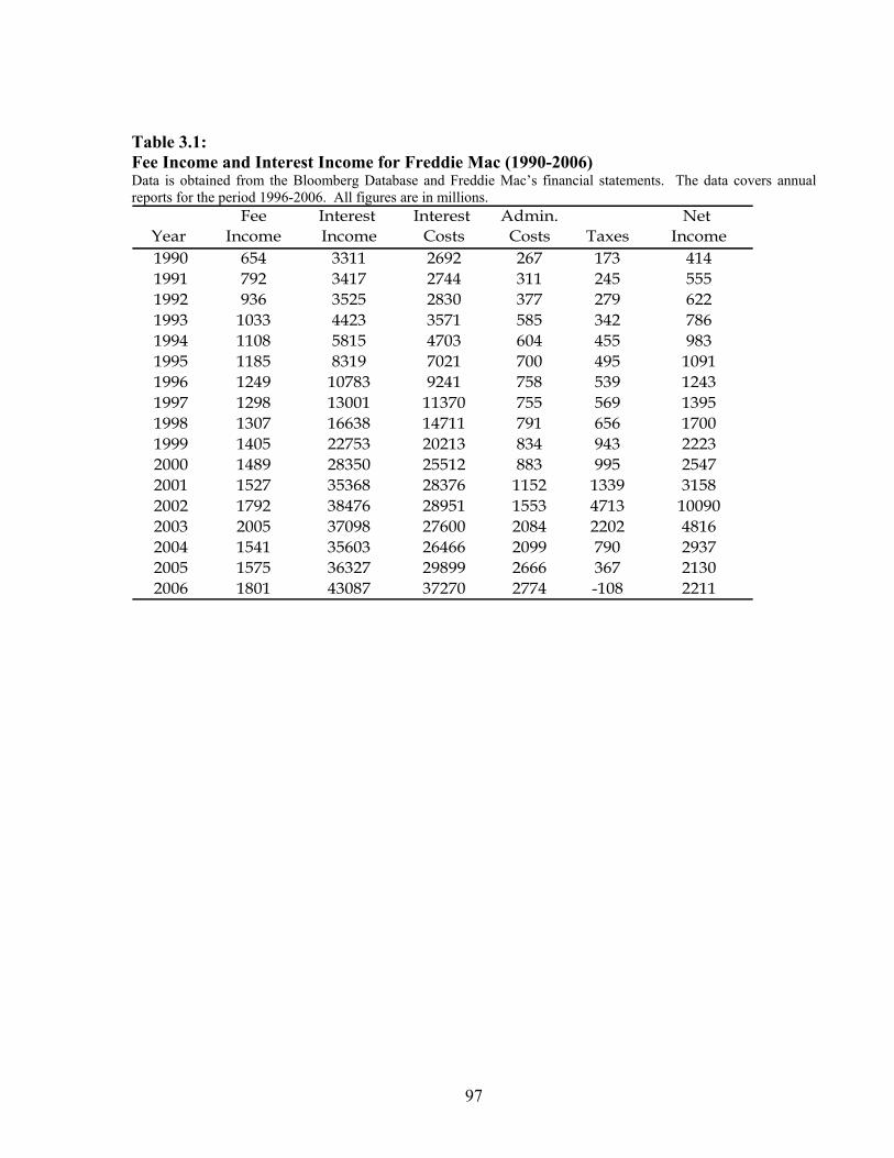
97

Table 3.1: Fee Income and Interest Income for Freddie Mac (1990-2006) Data is obtained from the Bloomberg Database and Freddie Mac’s financial statements. The data covers annual reports for the period 1996-2006. All figures are in millions.

Fee Interest Interest Admin. Net Year Income Income Costs Costs Taxes Income1990 654 3311 2692 267 173 4141991 792 3417 2744 311 245 5551992 936 3525 2830 377 279 6221993 1033 4423 3571 585 342 7861994 1108 5815 4703 604 455 9831995 1185 8319 7021 700 495 10911996 1249 10783 9241 758 539 12431997 1298 13001 11370 755 569 13951998 1307 16638 14711 791 656 17001999 1405 22753 20213 834 943 22232000 1489 28350 25512 883 995 25472001 1527 35368 28376 1152 1339 31582002 1792 38476 28951 1553 4713 100902003 2005 37098 27600 2084 2202 48162004 1541 35603 26466 2099 790 29372005 1575 36327 29899 2666 367 21302006 1801 43087 37270 2774 -108 2211

98

Table 3.2: Outstanding Debt and MBS holdings for Fannie Mae and Freddie Mac Data is obtained from the Bloomberg Database and the Department of Housing and Urban Development’s Office of Federal Housing Enterprise Oversight, the Federal Housing Finance Board and Fannie Mae’s and Freddie Mac’s financial statements.

D ateM B S D ebt M B S D ebt

1985 55 94 100 131986 96 94 169 151987 136 97 213 201988 170 105 226 271989 217 116 273 261990 288 123 316 311991 355 134 359 301992 424 166 408 301993 471 201 439 501994 486 257 461 931995 513 299 459 1201996 548 331 473 1571997 579 370 476 1731998 637 460 478 2871999 679 548 538 3612000 707 643 576 4272001 859 763 653 5782002 1,029 851 749 6662003 1,300 962 773 7402004 1,403 945 852 732

Fannie M ae Freddie M ac

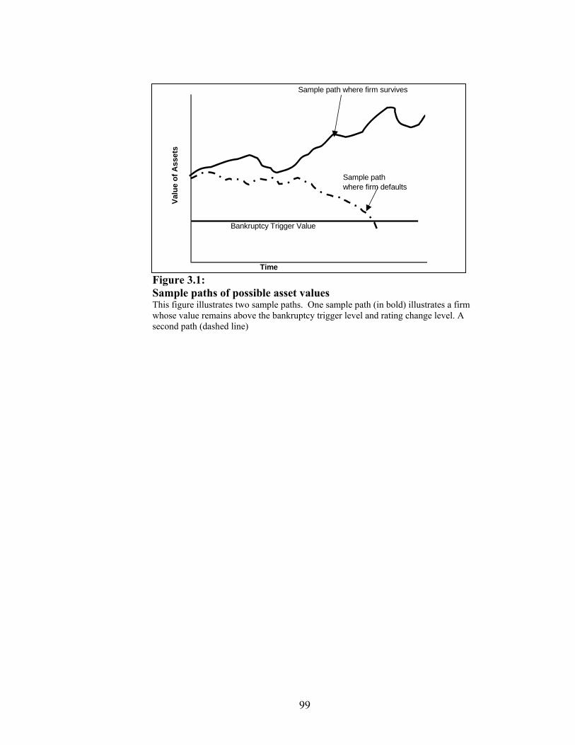
99

Figure 3.1: Sample paths of possible asset values This figure illustrates two sample paths. One sample path (in bold) illustrates a firm whose value remains above the bankruptcy trigger level and rating change level. A second path (dashed line)

Sample path where firm survives

Sample pathwhere firm defaults

Bankruptcy Trigger Value

Time

Valu

e of

Ass

ets

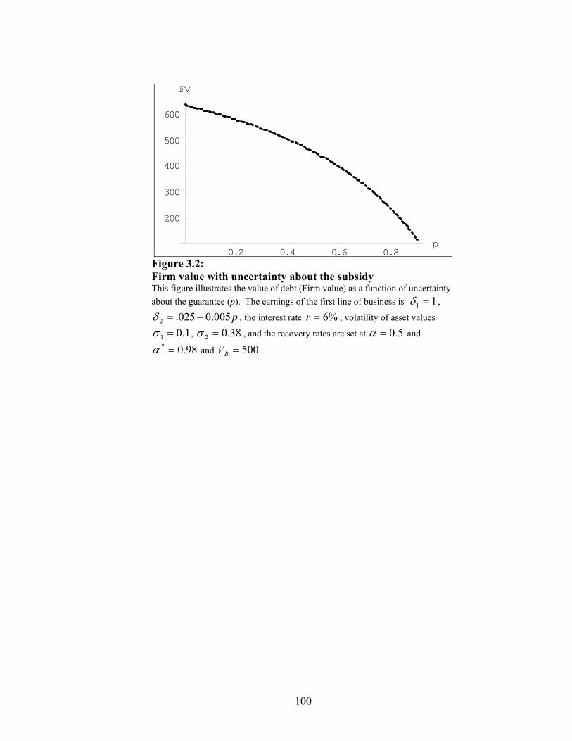
100

0.2 0.4 0.6 0.8p

200

300

400

500

600

FV

Figure 3.2: Firm value with uncertainty about the subsidy This figure illustrates the value of debt (Firm value) as a function of uncertainty about the guarantee (p). The earnings of the first line of business is 11 =δ ,

p005.0025.2 −=δ , the interest rate %6=r , volatility of asset values

1.01 =σ , 38.02 =σ , and the recovery rates are set at 5.0=α and

98.0* =α and 500=BV .

101

0.2 0.4 0.6 0.8p

400

450

500

550

DV

Figure 3.3: Debt value with uncertainty about the subsidy This figure illustrates the value of debt (Debt value) as a function of uncertainty about the guarantee (p). The earnings of the first line of business is 11 =δ , p005.0025.2 −=δ ,

the interest rate %6=r , volatility of asset values 1.01 =σ , 38.02 =σ , and the

recovery rates are set at 5.0=α and 98.0* =α and 500=BV .

No increase in hedging costs

With increase in hedging costs

102

0.2 0.4 0.6 0.8p

-200

200

400

EV and DV

Figure 3.4: Equity value and Debt Values with uncertainty about the subsidy This figure illustrates the value of debt (DV) and Equity (EV) as a function of uncertainty about the guarantee (p). The earnings of the first line of business is 11 =δ , p005.0025.2 −=δ ,

the interest rate %6=r , volatility of asset values 1.01 =σ , 38.02 =σ , and the recovery

rates are set at 5.0=α and 98.0* =α and 500=BV .

DV

EV

103

APPENDIX 2.A: WEALTH COMPONENTS

Human capital or Labor income wealth

Human capital is an unobservable variable; therefore a proxy is needed in order to

analyze human capital’s effect on returns. In the spirit of Campbell (1996) and Jagannathan and

Wang (1996), I assume that the return to human capital is of the following form:

t

ttthc HC

YHCR 11

1,++

+

+= (A.1)

where HCt corresponds to human capital and Yt is labor income, a dividend to human capital, all

in time t. Taking logs of both sides of equation (A.1) and rearranging terms gives:

)1log(1

111,

+

+++ ++−=

t

tttthc HC

Yhchcr . To simplify, I apply a first order Taylor expansion to log-

linearize the last term of the previous equation. Following Lettau and Ludvigson (2001a), the

log-linearization was made around a steady state, where the labor income-human capital

ratio,HCY , is assumed constant. By solving forward and assuming that

0)()1(lim =− ++∞→ ititi

i yhcω

, the resulting approximation comes to:

ttt zyhc ++=η (A.2)

where ∑∞

=++

− −Δ=1

,1 )()1(

iithcit

it ryz

ω,

HCY

+=

1

11ω

is a number between 0 and 1, and η is a

constant. Just as in Lettau and Ludvigson (2001a), zt is a mean zero stationary variable, therefore

it will not be included in this analysis. The lower case letters of equation (A.2) represent

logarithms of the variables of human capital, hct, and labor income, yt. Since human capital is

104

not observable, and using equation (A.2), it is assume that this wealth component can instead be

defined by aggregate labor income. To avoid confusion with subscripts, returns to human capital

are stated as 1, +tYR for the remainder of the article.

I compute labor income as wages and salaries plus transfer payments minus personal

contributions for social insurance minus taxes (a more detailed explanation can be found in the

appendix 2.B).

Debt interest payments (Debt wealth)

Following Hall (2001), the nonfarm nonfinancial business’ market value of debt, MVDt,

is computed as financial liabilities, FLt, plus total market value of bonds, MVBt, minus total book

value of bonds, BVBt, minus financial assets, FAt. Total book and market values of bonds are

adjusted for the value of tax exempt securities. Therefore,

)()( ttttt BVBMVBFAFLMVD −+−= .

I assume that newly issued bonds have coupons as if they were non-callable ten-year

bonds. MVBt is computed as the present value of the remaining future coupons of all the bonds

issued previously, C, and principal payments on the outstanding assigned bond issues. A bond’s

coupon rate at time t is assumed to equal to such bond’s yield to maturity at time t.

To calculate the present value of principal payments at time t, I discount the value of

newly issued bonds created within the previous 10 years to time t. But first I have to obtain the

value of newly issued bonds for every period as follows. Newly issued bonds, NIt, at time t

equals the net increase in the book value of bonds at time t plus the principal repayments made at

time t from bonds issued previously. Therefore, ttt repaymentsincipalBVNI Pr+Δ= , where

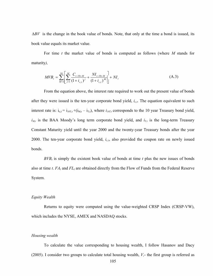
105

BVΔ is the change in the book value of bonds. Note, that only at the time a bond is issued, its

book value equals its market value.

For time t the market value of bonds is computed as follows (where M stands for

maturity),

tM

M

jM

tc

Mtj

tc

Mtt NI

iNI

iC

MVB +⎥⎥⎦

⎤

⎢⎢⎣

⎡

++

+= ∑ ∑

= =

+−+−10

1 1 ,

10

,

10

)1()1( (A.3)

From the equation above, the interest rate required to work out the present value of bonds

after they were issued is the ten-year corporate bond yield, ic,t. The equation equivalent to such

interest rate is: ic,t = i10T,t +(iM,t – iT,t), where i10T,t corresponds to the 10 year Treasury bond yield,

iM,t is the BAA Moody’s long term corporate bond yield, and iT,t is the long-term Treasury

Constant Maturity yield until the year 2000 and the twenty-year Treasury bonds after the year

2000. The ten-year corporate bond yield, ic,t, also provided the coupon rate on newly issued

bonds.

BVBt is simply the existent book value of bonds at time t plus the new issues of bonds

also at time t. FAt and FLt are obtained directly from the Flow of Funds from the Federal Reserve

System.

Equity Wealth

Returns to equity were computed using the value-weighted CRSP Index (CRSP-VW),

which includes the NYSE, AMEX and NASDAQ stocks.

Housing wealth

To calculate the value corresponding to housing wealth, I follow Hasanov and Dacy

(2005). I consider two groups to calculate total housing wealth, V,- the first group is referred as

106

owners,O, and the second group as rentiers, RNT,. Owners own and live in their homes, while

rentiers own their homes and rent these to someone else. Let Vo equal the total equity value

(assets minus debt) of owner homes and VRNT equal the total equity value of renters’ residences.

The formula of total housing wealth is the following: RNTVVV += 0 . Data on the value of

residential real estate for each group is taken from the Flow of Funds Accounts released by the

Federal Reserve. Owners’ housing wealth corresponds to household real estate minus total home

mortgages, and rentiers’ housing wealth corresponds to nonfarm noncorporate business

residential real estate minus total mortgages.

107

APPENDIX 2.B: DATA

I need five primary ingredients to conduct my empirical tests- aggregate consumption,

housing wealth, market value of debt, labor income and market value of equity as well as returns

to equity.

I use quarterly observations on the financial time-series for the United States over the

period of 1959 to 2006. This information is compiled by CRSP, the Federal Reserve, the Census

Bureau and the Bureau of Economic Analysis databases.

For comparison purposes with my work, I use Lettau and Ludvigson’s (2001a) consumption-to-

wealth ratio (cay), Quijano’s (2007) consumption-to-wealth ratio measure (cedy) which includes

only debt, equity and labor income in the wealth definition, dividend yield, dividend to earnings

ratio, term structure of interest rates, and short term interest rates as alternative predictive

measures of equity returns.

The dividend data was obtained from Professor Shiller’s website

(http://www.econ.yale.edu/~shiller/data/ie_data.xls). The Lettau and Ludvigson’s consumption-

to-wealth measure, cay, was calculated following the procedure stated in their (2001a) paper.

The term structure of interest rates was calculated as the spread between the 10 year Treasury

bond yield and the three month Treasury bill yield. The short term interest measure is simply the

three month Treasury bill minus its previous year average; Campbell (1987) called this measure

a stochastically detrended interest rate. Treasury bonds and bill’s data was obtained from the

Federal Reserve database.

As in Lettau and Ludvigson (2001a), labor income is calculated as “wages and salaries

plus transfer payments plus other labor income minus personal contributions for social insurance

108

minus taxes. Taxes are defined as (wages and salaries/ (wages and salaries + proprietors income

with IVA and Ccadj + rental income + personal dividends + personal interest income)) times

(personal tax and non-tax payments), where IVA is inventory evaluation and Ccadj is capital

consumption adjustments” (p.845). As an alternative, I also use Jagannathan and Wang (1996)

definition of labor income, which equals the growth in total personal per capita income less

dividend payments from the National Income and Product Accounts24. All labor income

components are published by the Bureau of Economic Analysis.

Equity value, debt value, housing wealth and other information needed to test my

hypotheses are calculated as follows.

The stock of outstanding equity is equal to the total market value of NYSE-AMEX-

NASDAQ stocks obtained from CRSP database. Returns are computed using the value-weighted

CRSP Index (CRSP-VW).

The data on the value of residential real estate for owners and rentiers is taken from the

Flow of Funds Accounts published by the Federal Reserve. Owners and rentiers’ residential real

estate data was taken specifically from tables B.100 (Balance Sheet of Households and Nonprofit

Organizations, line 49) and B.103 (Balance Sheet of Nonfarm Noncorporate Business, line 4

minus line 16), respectively. Owners’ housing wealth corresponds to household real estate minus

total home mortgages, and rentiers’ housing wealth corresponds to nonfarm noncorporate

business residential real estate minus total mortgages.

To calculate debt interest payments, I used principal repayments, book value of bonds

(corporate and tax exempt), financial assets and financial liabilities series, which were obtained

from the Federal Reserve Flow of Funds accounts. The 10 year Treasury bond yields and three-

24 Results are qualitatively similar when compared to Lettau and Ludvigson’s measure of labor income.

109

month Treasury bill yields were obtained from the Federal Reserve database. The Federal

Reserve database also publishes Moody’s long-term corporate bond yields (with a BAA grade),

the long-term Treasury Constant Maturity Composite yield, and the twenty-year Treasury bond

yields. I use the long-term Treasury Constant Maturity Composite yield for the quarterly period

from 1959 until 2000 and then substitute it with the twenty-year Treasury bonds after the year

2000, because the long-term Treasury Constant Maturity was discontinued.

Consumption data was collected from the Bureau of Economic Analysis. Total

consumption used for this paper is simply the sum of non-durable goods and services minus

clothing and shoes from personal consumption expenditures. Clothing and shoes are excluded

from this measure, since some consider them as durable consumption goods (Duffee (2003)).

Figure 1 illustrates the consumption growth - it highly fluctuates in a small range of values

resulting in a low standard deviation. Nevertheless, in futures sections, I’ll demonstrate that even

though consumption growth looks very stable, it carries important implications for the analysis

of expected stock returns.

All data is in real terms and was deflated by the PCE chain-type price deflator, 1992 =

100. Data on consumption, equity, debt, housing and labor income are in per capita terms; the

estimates for population were obtained from the Census Bureau. Table I reports summary

statistics for consumption, debt, equity, housing and labor income per capita.

110

APPENDIX 2.C: CAMPBELL AND YOGO (2006) PRETESTS

Campbell and Yogo (2006), building upon previous work by Lewellen (2003) and

Stambaugh (1999), argue that some of the evidence in favor of predictability of stock returns is

the result of incorrect inference. They show that if the variable used to predict returns is near-

integrated and if the innovations in this variable are sufficiently correlated to the innovations in

stock returns, then traditional statistical tests lead to biased results. In particular, the usual t

statistic, testing for statistical significance in a regression of future stock returns on a predictor

variable, will lead to spurious rejection of the null hypothesis of no significance too many times,

and inference based on this test will show predictability of stock returns when in fact there is

none. Campbell and Yogo call this a size distortion, because the size of the test (the so called

type I error) is much larger than that assumed by the researcher.

Campbell and Yogo (2006) develop a simple pretest based on the confidence interval for

the largest autoregressive root of the predictor variable. In summary, if the confidence interval

indicates that the predictor variable is adequately stationary, for a given level of correlation

between the innovations to returns and the predictor variable, then one can proceed with and

accept the inference based on the standard t-test with conventional critical values. Campbell and

Yogo’s pretest just diagnostics if conventional t-tests suffer from a size distortion, loosely

speaking a 95% confidence interval may in fact be substantially lower. They conclude that

persistence in a predictor variable is not a problem as long as their innovations have sufficiently

low correlation with the innovations to stock returns.

I estimate Campbell and Yogo’s (2006) pretest to test the validity of the t-tests obtained

from the in-sample regressions that show of the explanatory power on stock returns when using

111

u-ccw. I compare my results about inference on t-tests with those estimated using Lettau and

Ludvigson’s (2001a) cay, the dividend to price ratio, and the stochastically detrended short

interest rate.

The pretest provides simple proof on true inference of forecasting models. To calculate

the pretest for a variable (in my case: u-ccw) that is attempting to predict stock returns, rE,t+1,

then the following regressions have to be performed,

t

tE

eccwubbccwu

vccwuaar

+−+=−

+−+=

1-tt

t1-t

21

21, , (C.1)

In summary, to perform the pretest one has to follow the next few steps:

1) Estimate equations (C.1) using seemingly unrelated regressions. Then calculate the correlation

coefficient, ρv,e between vt and et.

2) Obtain the autoregressive coefficient for the predictor variable, b2, using the Dickey Fuller-

GLS method of Elliot et al (1996).

3) Once having the estimates of the correlation between the residuals from equations (C.1) and

the autoregressive coefficient for u-ccw, use these results to create an interval for a parameter c

and compare this interval to a critical interval given in Campbell and Yogo (2006). If any part of

the interval for c is not contained in the critical interval, then the result of the pretest is that

inference based on the usual t-test is correct.

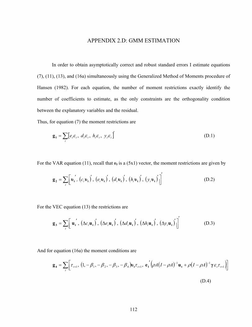
112

APPENDIX 2.D: GMM ESTIMATION

In order to obtain asymptotically correct and robust standard errors I estimate equations

(7), (11), (13), and (16a) simultaneously using the Generalized Method of Moments procedure of

Hansen (1982). For each equation, the number of moment restrictions exactly identify the

number of coefficients to estimate, as the only constraints are the orthogonality condition

between the explanatory variables and the residual.

Thus, for equation (7) the moment restrictions are

[ ]∑ ′=t

tttttttt yhde εεεε ,,,1g (D.1)

For the VAR equation (11), recall that υt is a (5x1) vector, the moment restrictions are given by

( ) ( ) ( ) ( ) ( )∑′

⎥⎦⎤

⎢⎣⎡ ′′′′′′=

tttttt yhdec, tttttt2 υυυυυυg ,,,, (D.2)

For the VEC equation (13) the restrictions are

( ) ( ) ( ) ( ) ( )∑′

⎥⎦⎤

⎢⎣⎡ ′Δ′Δ′Δ′Δ′Δ′=

tttttt yhdec tttttt3 uuuuuug ,,,,, (D.3)

And for equation (16a) the moment conditions are

( ) ( ) ( )( )∑ ⎥⎦⎤

⎢⎣⎡ −+−′−−−−= +

−−++

ttttt AIAIA 1

11143211 ,,,,,1, τερρρρτββββτ γueυg t1t4

(D.4)

113

The efficient GMM estimation then minimizes the following quadratic objective function over

the parameter space Θ

⎪⎭

⎪⎬⎫

⎪⎩

⎪⎨⎧ ′

⎥⎦⎤

⎢⎣⎡ ′′′′

⎥⎦⎤

⎢⎣⎡ ′′′′

Θ 43214321 g,g,g,gg,g,g,g Wmin (D.5)

where W is the optimal nonnegative weighting matrix as described in Newey and West (1987b).

Finally, the variance-covariance matrix of the coefficient vector θ is computed as

( )1

ˆvar

−

⎟⎟⎟⎟

⎠

⎞

⎜⎜⎜⎜

⎝

⎛

∂

′

⎥⎦⎤

⎢⎣⎡ ′′′′∂

∂⎥⎦⎤

⎢⎣⎡ ′′′′∂

=θ

g,g,g,g

θ

g,g,g,gθ

43214321W (D.6)

114

APPENDIX 3.A: BACKGROUND ON F&F

This section describes the business of as Fannie Mae and Freddie Mac 25. F&F are financial

intermediaries created by the Congress of the United States to create liquidity in the housing loan

market, and to fund loans to certain groups of borrowers such as homeowners, farmers and

students. Fannie Mae was originally created as a wholly owned government corporation in 1938

and was converted into a F&F in 1968. Freddie Mac was created in 1970 as part of the Federal

Home Loan Bank System to purchase mortgages from thrifts. Rather than hold mortgages in its

portfolio, Freddie Mac pooled these mortgages and sold them after attaching a guarantee for

credit risk.

As noted in the introduction, F&F are hybrids of private corporations and federal entities.

The F&F are chartered by a federal statute and are exempt from state and local taxes, registration

requirements. The US treasury is authorized to lend $2.25 billion to each of them. Banks are

allowed to make unlimited investments in F&F debt securities, and F&F securities are eligible as

collateral for public deposits as well as for Treasury tax and loan accounts. Also, F&F are

exempt from the provisions of many state investor protection laws.

The low spread on F&F debt coupled with the rapid growth of F&F has focused attention

on their impact on the systemic risk of the financial markets. Although the debt securities issued

by the F&F explicitly state that they do not carry a federal guarantee, their ties to the federal

government convince investors of their ties to the federal government and the low risk of their

debt.

25 We adapt this information from other published descriptions of these entities.

115

Table 1 gives the outstanding debt of Fannie Mae and Freddie Mac. Their combined

holding of mortgage backed securities as well as the amount of debt has grown to over or near 2

trillion dollars. Market participants as well as regulators increasingly want to determine how

the size of the assets and liabilities is likely to affect the chance that the government may need to

bail them out (value of the government subsidy). The uncertainty about the guarantee,

addressed in this article, also leads to answers about how the implicit subsidy impacts the value

of the firm and that of equity, and if the government ought to fix the potential liability of tax

payers at the outset.

116

APPENDIX 3.B: PROOF FOR REMARK 1 AND 2

From Leland (1994), the present value of coupon payments is:

( )[ ] =−∫∞

−

00 ,,1 dtVVtFCe B

rt

⎟⎟

⎠

⎞

⎜⎜

⎝

⎛⎥⎦

⎤⎢⎣

⎡−

−x

BVV

rC 01 where

⎥⎥

⎦

⎤

⎢⎢

⎣

⎡+⎟⎟

⎠

⎞⎜⎜⎝

⎛−+⎟⎟

⎠

⎞⎜⎜⎝

⎛−= 2

222

2 222

1 σσσσ

rrrx and

( )TVVtF ,, 0 is the density of the first passage time of the firm value from 0V to BV . Also the

present value of payoffs were the firm to go bankrupt is given by ( )∫∞

−

00 ,, dtVVtgVe BB

rtα and is

evaluated as: [ ]x

BB V

VV

−

⎥⎦

⎤⎢⎣

⎡ 0α . The sum of these payments gives the desired result for Remark 2.

Similarly, Firm value is equal to the unlevered firm value )( 0V , plus tax benefits

⎟⎟

⎠

⎞

⎜⎜

⎝

⎛⎥⎦

⎤⎢⎣

⎡−

−x

BVV

rC 01τ , and minus bankruptcy costs with a probability

x

BVV

−

⎥⎦

⎤⎢⎣

⎡ 0 .

117

BIBLIOGRAPHY

(2001), Federal subsidies and the housing GSEs, (Congressional Budget Office). Alvarez, F., and U. Jermann, (2000). Asset pricing when risk sharing is limited by default. Econometrica, Vol.68, pp.775–98. Ambrose, B. W., and A. Warga, (2002). Measuring Potential GSE Funding Advantages, Journal of Real Estate Finance and Economics, Vol.25, pp.129-150. Black, F., and J. C. Cox, (1976). Valuing corporate securities: Some effects on bond indenture provisions, Journal of Finance, Vol.31, pp.351-367. Black, F., and M. Scholes, (1973). The pricing of options and corporate liabilities, Journal of Political Economy, Vol. 81, pp.637-659. Breeden, D.T., (1979). An intertemporal asset pricing model with stochastic consumption and investment opportunities. Journal of Financial Economics, Vol. 7, pp.265-296. Campbell, J.Y., (1987). Stock Returns and the Term Structure. Journal of Financial Economics, Vol.18, pp.373–399. Campbell, J.Y., (1996). Understanding Risk and Return. Journal of Political Economy, Vol.104, pp.298–345, Campbell, J.Y., and J.H. Cochrane, (1999). By Force of Habit: A Consumption-Based Explanation of Aggregate Stock Market Behavior. Journal of Political Economy, Vol.107 (2), pp.205-251. Campbell, J.Y., and R. J. Shiller, (1988). Valuation ratios and the long-run stock market outlook. Journal of Portfolio Management, Vol. 24, pp.11−26. Campbell, J.Y., A.W. Lo, and A.C. MacKinlay, (1997). The Econometrics of Financial Markets. Princeton University Press, Princeton, New Jersey. Campbell, J. Y., and G. Mankiw, (1989) Consumption, income and interest rates: Reinterpreting the time series evidence, Working Paper, National Bureau of Economic Research. Campbell, J.Y., and M. Yogo, (2006). Efficient Tests of Stock Return Predictability. Journal of Financial Economics, Vol. 81, pp.27-60. Cecchetti, S. G., and N. Mark, (1990). Evaluating Empirical Tests of Asset Pricing Models: Alternative Interpretations. The American Economic Review, Vol. 80 (2), pp.48-51.

118

Chang, G., and S. Sundaresan, (2005) Asset Prices and Default-Free Term Structure in an Equilibrium Model of Default, Journal of Business, Vol.78 (3), pp.997-1021. Chen, N., R. Roll, and S. Ross, (1986). Economic forces and the stock market. Journal of Business, Vol. 59, pp.383–403. Chen, N., (1991). Financial investment opportunities and the macro-economy. Journal of Finance, Vol. 46, pp.529–54. Cochrane, J. (2005), Asset Pricing (Revised), Princeton: Princeton University Press, New Jersey. Cooper, I. A., and A. S. Mello, (1992). The Default Risk of Swaps, Journal of Finance, Vol. 47, pp.597-620. Constantinides, G.M. (1990). Habit Formation: A Resolution of the Equity Premium Puzzle. Journal of Political Economy, Vol.98 (3), pp.519-543. Constantinides, G.M., J.B. Donaldson, and R. Mehra, (2002). Junior can’t borrow: a new perspective on the equity premium puzzle. Quarterly Journal of Economics, Vol.118, pp.269−296. Diebold, F. and R. Mariano, (1995). Comparing Predictive Accuracy. Journal of Business and Economic Statistics, Vol. 13, pp.253-263 Duffee, G., (2005) Time Variation in the Covariance between Stock Returns and Consumption Growth. Journal of Finance, Vol. 60 (4), pp.1673-1712. Duffie, D., and K. Singleton, (1997). An Econometric Model of the Term Structure of Interest Rate Swap Yields. Journal of Finance, Vol. 52, pp.1287-1323 Duffie, D., and K. Singleton, (1999). Modeling Term Structures of Defaultable Bonds. Review of Financial Studies, Vol. 12, pp.687-720 Epstein, L.G., and S.E. Zin, (1989): Substitution, Risk Aversion, and the Temporal Behavior of Consumption and Asset Returns: A Theoretical Framework. Econometrica, Vol.57 (4), pp.937-969. Epstein, L.G., and S.E. Zin, (1990). ‘First-Order’ Risk Aversion and the Equity Premium Puzzle. Journal of Monetary Economics, Vol. 26, pp.387-407. Epstein, L.G., and S.E. Zin, (1991). Substitution, Risk Aversion, and the Temporal Behavior of Consumption and Asset Returns: An Empirical Analysis. Journal of Political Economy, Vol. 99 (2), pp.263-286. Fama, E., and K. French, (1988). Permanent and Temporary Components of Stock Prices. Journal of Political Economy, Vol. 96(2), pp. 246-274.

119

Fama, E., and K. French, (1988). Dividend Yields and Expected Stock Returns. Journal of Financial Economics, Vol. 22, pp.3-25. Fama, E., and K. French, (1989). Business conditions and the expected returns on bonds and stocks. Journal of Financial Economics, Vol. 25, pp.23–50. Fama E., and J. MacBeth, (1973). Risk, Return, and Equilibrium: Empirical Tests, Journal of Political Economy, Vol. 81, pp.607-636. Ferson, W. E., and C. R. Harvey, (1991). The variation of economic risk premiums. Journal of Political Economy, Vol. 99, pp.385–415. Goldstein, R., N. Ju, and H. Leland, (2001). An EBIT-based model of dynamic capital structure, Journal of Business, Vol. 74, pp.483-512. Goyal, A. and I. Welch, (2003) Predicting the Equity Premium with Dividend Ratios. Management Science, Vol. 49 (5), pp.639-654. Goyal, A. and I. Welch, (2006) A Comprehensive Look at the Empirical Performance of Equity Premium Prediction, Working Paper No. 04-11, Yale School of Management, International Center of Finance, Connecticut. Hall, R., (2001). The Stock Market and Capital Accumulation. American Economic Review, Vol. 91, pp.1185-1202. Harvey, D. I., S. J. Leybourne, and P. Newbold, (1998). Tests for Forecast Encompassing. Journal of Business and Economic Statistics, Vol. 16, pp.254-259 Hansen, L.P., (1982). Large Sample Properties of Generalized Method of Moments Estimators. Econometrica, Vol. 50, pp.1029-1054. Hasanov, F., and D. Dacy, (2005). Measuring and Analyzing Returns on Aggregate Residential Housing, Econ WPA – Finance series # 0510005. Hubbard, G. R., (2004). The relative risk of Freddie and Fannie, Fannie Mae papers 3. Jaffee, D., (2003). The interest rate risk of Fannie Mae and Freddie Mac, Journal of Financial Services Research, Vol. 24, pp.5-29. Jagannathan, R., and Z. Wang, (1996). The conditional CAPM and the cross-section of expected returns. Journal of Finance, Vol. 51, pp.3–53. Jarrow ,R.A., and S. Turnbull, (1995). Pricing Derivatives on Financial Securities Subject to Credit Risk. Journal of Finance, Vol. 50, pp.53-85.

120

Julliard, C. (2004), Labor income risk and asset returns, Manuscript, Princeton University, New Jersey. Keim, D. B., and R. F. Stambaugh, (1986). Predicting returns in the stock and bond markets. Journal of Financial Economics, Vol. 17, pp.357–90. Lehnert, A., and S. W. Passmore, (2006). Comment on: "An options-based approach to evaluating the risk of Fannie Mae and Freddie Mac", Journal of Monetary Economics, Vol. 53, pp.177-182. Lehnert, A., W. Passmore, and S. M. Sherlund, (2006). GSEs, Mortgage Rates, and Secondary Market Activities, Federal Reserve Board, Finance and Economics Discussion Series pp.2006 2030. Leland, H. E., (1994). Corporate debt value, bond covenants and optimal capital structure, Journal of Finance, Vol. 51, pp.1231-1252. Leland, H. E., (1994). Bond prices, yield spreads, and optimal capital structure with default risk, Working Paper, University of California, Berkeley. Lettau, M., and S. Ludvigson, (2001a) Consumption, aggregate wealth and expected stock returns. Journal of Finance, Vol. 55, pp.815–849. Lettau, M., and S. Ludvigson, (2001b) Resurrecting the (C)CAPM: A cross-sectional test when risk premia are time-varying, Journal of Political Economy, Vol.109(6), pp.1238-1287. Longstaff, F., and E. Schwartz, (1995). Valuing Risky Debt: A New Approach. Journal of Finance, Vol. 50, pp.789-820. Lucas, R. E., (1978). Asset Prices in an Exchange Economy. Econometrica, Vol. 46, pp.1429-1445. Lucas, D., and R. McDonald, (2006). An Option-Based Approach to Evaluating the Risk of Fannie Mae and Freddie Mac, Journal of Monetary Economics, Vol. 53, forthcoming. McGrattan, E.R., and E.C. Prescott, (2000). Is the market overvalued? Federal Reserve Bank of Minneapolis Quarterly Review, Vol. 24, pp.20−40. McGrattan, E.R., and E.C. Prescott, (2001). Taxes, regulations, and asset prices. Working Paper 610, Federal Reserve Bank of Minneapolis. Mehra, R. and E.C. Prescott, (1985). The Equity Premium: A Puzzle. Journal of Monetary Economics, Vol. 15, pp.145-161. Mehra, R., and E.C. Prescott, (1988). The equity premium: a solution? Journal of Monetary Economy, Vol. 22, pp.133−136

121

Merton, R. C., (1974). On the pricing of corporate debt: The risk structure of interest rates, Journal of Finance, Vol. 29, pp.449-470. Modigliani, F., and M. Miller, (1958). The Cost of Capital, Corporation Finance and the Theory of Investment. American Economic Review, Vol.48, pp.261-197 Newey, W., and K. West, (1987a). Hypothesis Testing with Efficient Method of Moments Estimation. International Economic Review, Vol. 28, pp.777–787. Newey, W., and K. West, (1987b). A Simple Positive Semi-definite, Heteroskedasticity and Autocorrelation Consistent Covariance Matrix. Econometrica, Vol. 55, pp.703–708. Naranjo, A., and A. L. Toevs, (2002). The effects of purchases of mortgages and securitization by Government Sponsored Enterprises on mortgage yield Spreads and volatility, The Journal of Real Estate Finance and Economics, Vol. 25. Nothaft, F. E., J. E. Pearce, and S. Stevanovic, (2002). Debt Spreads Between GSEs and Other Corporations, Journal of Real Estate Finance and Economics, Vol. 25. Passmore, W., (2005). The GSE implicit subsidy and the value of government ambiguity, Real Estate Economics, Vol. 33, pp.465-486. Piazzesi, M., M. Schneider, and S. Tuzel, (2007), Housing, consumption, and asset pricing, Journal of Financial Economics, Vol. 83(3), pp.531-569. Rietz, T.A., (1988). The Equity Risk Premium: A Solution, Journal of Monetary Economics Vol. 22(1), pp.117-131. Rouwenhorst, G.K., (1995), Asset Pricing Implications of Equilibrium Business Cycle Models. in Frontiers of Business Cycle Research, ed. by T.H. Cooley, Princeton University Press, Princeton, New Jersey, pp.294-330 Santos, T., and P. Veronesi, (2005) Labor income and predictable stock returns, Working Paper, University of Chicago Graduate School of Business, Chicago. Seiler, R. S., (2003). Market discipline of Fannie Mae and Freddie Mac: How do share prices and debt yield spreads respond to new information?, OFHEO Working paper. Stiglitz, J. E., J. M. Orsag, and P. Orsag, (2002). Implications of the new Fannie Mae and Freddie Mac risk based capital standards, Fannie Mae papers 1. Vassalou, M., and Y. Xing, (2004). Default Risk in Equity Return, Journal of Finance, Vol. 59, pp.831-868.

122

Vassalou, M., J. Chen, and L. Zhou, (2005). The interrelation of Liquidity Risk, Default Risk, and Equity Returns, Working Paper, Columbia University, New York. Wachter, J. A., (2002) Habit formation and returns on bonds and stocks, Working paper FIN- 01-024, New York University, Stern School of Business, New York. Zame, W. R., (1993). Efficiency and the role of default when security markets are incomplete. American Economic Review, Vol. 83, pp.142–64. Zhang, H., (1997). Endogenous borrowing constrains with incomplete markets, Journal of Finance, Vol. 52, pp.2187–2209.

VITA

Margot Claudette Quijano was born on March 12, 1980, to Alicia Cantu de Quijano and

Ruy A. Quijano in Albuquerque, New Mexico, U.S.A. In May 2002, she received the degree of

Bachelor in Arts in Economics from I.T.E.S.M. at Monterrey, Nuevo Leon, Mexico. In summer

2005, Margot worked as an intern in the Economic Policy Department at the U.S. Department of

the Treasury. Later, in August 2005, she was admitted to the Ph.D. program in Finance from the

College of Business at the University of Texas at San Antonio. Margot married Emmanuel

Alanis in December 2007. She has been working under the supervision of Dr. Karan Bhanot,

with whom she co-authored one working paper.