Essays in Open Economy Monetary Policy by Pedro Araujo...

Essays in Open Economy Monetary Policy

by

Pedro Araujo Castro

A dissertation submitted in partial satisfaction of the

requirements for the degree of

Doctor of Philosophy

in

Economics

in the

Graduate Division

of the

University of California, Berkeley

Committee in charge:

Professor Maurice Obstfeld, Chair

Professor Barry Eichengreen

Professor Yuriy Gorodnichenko

Professor Andrew Rose

Spring 2012

Abstract

Essays in Open Economy Monetary Policy

by

Pedro Araujo Castro

Doctor of Philosophy in Economics

University of California, Berkeley

Professor Maurice Obstfeld, Chair

International economic integration has risen during the last decades and the interde-pendence between each economy and the rest of the world has become central for policydecisions. My dissertation contributes to the debate about the conduct of monetarypolicy in a financially integrated world.

In the first chapter of the dissertation I discuss the relationship between domesticpolicies and the currency denomination of foreign debt. Foreign debt is a double-edgedsword. It allows countries to invest more than what would be possible given their ownsavings, thereby achieving preferable allocations that would not otherwise be feasible.However, it is the root of several crises. Foreign debt is especially hazardous whendenominated in foreign currency; in such cases exchange rate depreciations increase thereal value of the debt. An important question then is what determines the currencydenomination of foreign debt. I use the adoption of Inflation Targeting (IT) in severaleconomies during the last two decades to evaluate the importance of domestic policies inthe determination of the currency denomination of debt. In order to control for possibleendogeneity in IT adoption, I use matching and instrumental variables estimators; bothgenerate similar estimates. The results show that monetary policy can have substantialeffects on the amount of debt in foreign currency and that a more flexible exchange rateregime increases the use of domestic currency in foreign borrowing.

In the second chapter of the dissertation I investigate the relationship between centralbanks balance sheets and monetary policy. Heavy foreign exchange intervention by centralbanks of emerging markets have led to sizeable expansions of their balance sheets in recentyears - accumulating foreign assets and non-money domestic liabilities (the latter due tosterilization operations). With domestic liabilities being mostly of short-term maturityand denominated in local currency, movements in domestic monetary policy interest ratescan have sizable effects on central bank’s net worth. In this chapter I examine empiricallywhether balance sheets considerations influence the conduct of monetary policy. Themethodology involves the estimation of interest rate rules for a sample of 41 countriesand testing whether deviations from the rule can be explained by a measure of centralbank financial strength. My findings, using linear and nonlinear techniques, suggest thatcentral bank financial strength can be a statistically significant factor explaining largenegative interest rate deviations from “optimal” levels.

In the third chapter I investigate whether countries that adopted the IT frameworkfor monetary policy have been constrained by exchange rate consideration when takingpolicy decisions. I present stylized facts which suggest that exchange rates have been

1

allowed to float relatively free in IT countries. I employ Bayesian Analysis techniques toestimate a Dynamic Stochastic General Equilibrium (DSGE) structural model for twentytwo IT economies and compute posterior odds tests to check whether the central bankssystematically respond to exchange rate movements. The main result is that only fivecentral banks directly respond to exchange rate movements; all the other IT centralbanks do not respond to the exchange rate. I also confirm that IT central banks havebeen conducting strictly inflationary policies, raising real interest rates in response toincreases in inflation.

2

Dedication

To my Parents, Marcelo, Maiura, Alison, and Juliana.

i

Acknowledgments

I want to acknowledge support received from the Department of Economics at the Uni-versity of California, Berkeley, without which I could not complete my PhD. I am partic-ular grateful to my adviser, Professor Maurice Obstfeld, and to Professors Barry Eichen-green, Pierre-Olivier Gourinchas, Yuriy Gorodnichenko, Andrew Rose, David Romer,Demian Pouzo and Brad DeLong. Finally, I want to acknowledge support received frommy colleagues; I want to thank them for all these years spent together, the relationshipwe developed was invaluable for me.

ii

Introduction ∗

International economic integration has risen during the last decades and policy de-cisions now have to take into account the interdependence between each economy andthe rest of the world. My dissertation contributes to the debate about the conduct ofmonetary policy in a financially integrated world.

In the first chapter I discus the relationship between domestic policies and the currencydenomination of foreign debt. Foreign debt is a double-edged sword. It allows countriesto invest more than what would be possible given their own savings, thereby achievingpreferable allocations that would not otherwise be feasible. However, it is the root ofseveral crises, like the Latin America sovereign debt crises of the 1980s, the Mexican,Russian and Asian crises of the 1990s, and the current crisis in advanced economies,particularly in Europe.

The main distinguishing mark of foreign debt is the fact that borrowers and lendersmeasure their returns in different currencies, making their real returns move in oppositedirections when the exchange rate changes. Devaluations of the exchange rate increasethe debt overhang for borrowers when it is denominated in foreign currency, demandinglarge sacrifices in order to repay the debt.

The fact that most countries do not use their own currency when borrowing abroadhas led to a growing literature on the determinants of the currency denomination offoreign debt. However, there is no consensus about the role played by domestic policiesand, in particular, by monetary and exchange rate policies, on the pattern of foreignborrowing. The first chapter of my dissertation contributes to this literature in two ways.First, I show that domestic policies can influence the currency denomination of foreigndebt. I show this using the adoption of the Inflation Targeting (IT) framework in severalcountries during the past decade. Using a semi-parametric matching technique, I amable to show how this major change in the conduct of monetary policy has affected thecurrency denomination of foreign debt. Second, I show that the adoption of IT changedthe pattern of foreign borrowing due to the increase in exchange flexibility. In particular,countries that adopted IT and allowed their exchange rates to fluctuate more have beenable to use their domestic currency for foreign borrowing to a greater extent.

In the second chapter I discuss the relationship between central banks balance sheetsand monetary policy. Over the past decade, efforts to manage large capital inflowsby many central banks in emerging market (EM) countries have led to a major shift

∗Department of Economics, University of California, Berkeley. I am grateful to Maurice Obstfeldfor his support throughout my research. Barry Eichengreen, Pierre-Olivier Gourinchas, Yuriy Gorod-nichenko, Andrew Rose, David Romer, Demian Pouzo, Brad DeLong, and seminar participants at UCBerkeley provided valuable feedback.

iii

in the composition and size of their balance sheets. Significant foreign exchange (FX)intervention has been accompanied by large expansions of their net foreign assets aswell as domestic (interest-bearing) liabilities - with the latter reflecting large sterilizationoperations aimed at containing the monetary effects of FX interventions. As a result,currency mismatches in their balance sheets have widened. In parallel, central banks havewitnessed a secular decline in their capital - interrupted only temporarily by the effect ofthe sharp depreciations triggered by the 2008 global financial crises. Such dynamics areparticularly evident in emerging Asia, especially when the components of balance sheetsare measured relative to the country’s GDP. A breakdown between inflation targeting (IT)and non-inflation targeting regimes also reveals that capital losses have been particularlypronounced in the first group, as lower tolerance for inflation led to reduced seigniorageand revaluation losses from currency appreciation.

This transformation in central bank balance sheets (CBBS) has increased the sen-sitivity of capital to domestic interest rate movements. Indeed, the accumulation offoreign currency instruments on the asset side, along with short-term, local currency-denominated securities on the liability side increases the impact of movements in short-term domestic interest rates (i.e. monetary policy rates) on central banks’ capital. Thiseffects operates through two distinct channels: by affecting the amount of interest pay-ments on liabilities - while having no effect on the asset (revenue) side - and via exchangerate movements that derive in capital losses. The magnitude of this potential effect oncentral banks’ capital has grown over time, as balance sheets have expanded while capitalshrunk.

This background brings to the forefront of the policy debate the issue of whethercentral bank’s financial strength (CBFS) may affect the conduct of monetary policy. Ingeneral, whether a low degree of capital and/or high sensitivity to interest rate move-ments affects monetary policy decisions remains a relatively unexplored question in thetheoretical and empirical macroeconomic literature. In fact, there are (un-tested) op-posing views. Some argue that CBBS are irrelevant as central banks have the ability toprint money money to recapitalize themselves through seigniorage, or because ultimatelywhat matters are the institutional arrangements in place (i.e., recapitalization agreementswith the Treasury) and the consolidated fiscal position (i.e., fiscal ability to recapitalizethe central bank). By contrast, others argue that political economy reasons are enoughfor central banks to care about the health of their balance sheets, as financial weaknessmay trigger greater oversight and reduce independence, leading central banks to pursuesub-optimal policies in order to minimize the risk of losing independence.

In this chapter I assess empirically whether CBFS constraints monetary policy deci-sions. Although previous studies have explored the nexus between CBBS and macroeco-nomic outcomes, such as inflation, this constitutes the first attempt to study empiricallyand quantify the extent to which CBFS interferes with monetary policy decisions perse. I find evidence that a weak central bank balance sheet can influence the conductof monetary policy. Quite importantly, the relationship between central bank balancesheets and monetary policy is highly non-linear-i.e., large deviations from optimal policyare associated with very weak balance sheets.

In the third chapter I investigate whether countries that adopted the IT framework formonetary policy have been constrained by exchange rate consideration when taking policydecisions. Despite being a relatively new approach to monetary policy the IT framework

iv

is now fully implemented in twenty seven countries around the world. The frameworkis known for the public announcement of numerical values of an inflation target and thesubordination of all other policy objectives to its achievement. The empirical evidenceregarding its success is often positive and there is no evidence that it was harmful forits adopters. Also, its durability and the fact that it has been expanding without anycoordination led some to emphasize its relevance in shaping a new international monetarysystem.

This chapter aims to understand the role of the exchange rate in the IT regimes.IT requires nominal exchange rate flexibility; in an economy with unrestricted capitalflows, if the monetary policy is focused on domestic conditions the nominal exchangerate must be allowed to fluctuate. Despite this seemly simple requirement, discussionsabout the appropriate level and flexibility of the exchange rate are still central in thepolicy debate of IT economies and economists often disagree on the degree to which ITcentral banks actually respond to exchange rate movements. This chapter contributesto this debate in two ways. First, I present several stylized facts showing that exchangerates have been floating relatively free in IT economies; whether I compare the exchangerates of IT economies with those of non-IT ones or with their own exchange rates beforethe adoption of the framework the result is always that the adoption of IT is associatedwith greater exchange rate flexibility. I also show that interest rates in IT economies haveshowed lower variability than in non-IT ones. Second, I estimate a structural model andpay special attention to policy responses to exchange rate movements. I find that mostIT central banks do not directly respond to exchange rate movements, and confirm thefact that they have been conducting strictly anti-inflationary policies as assigned by theTaylor Principle.

v

Chapter 01What is the Role of Monetary and Exchange RateRegimes for the Currency Denomination of Foreign

Debt? ∗

Abstract

Foreign debt is a double-edged sword. It allows countries to invest more than whatwould be possible given their own savings, thereby achieving preferable allocations thatwould not otherwise be feasible. However, it is the root of several crises. Foreign debt isespecially hazardous when denominated in foreign currency; in such cases exchange ratedepreciations increase the real value of the debt. An important question then is whatdetermines the currency denomination of foreign debt. I use the adoption of InflationTargeting (IT) in several economies during the last two decades to evaluate the impor-tance of domestic policies in the determination of the currency denomination of debt. Inorder to control for possible endogeneity in IT adoption, I use matching and instrumentalvariables estimators; both generate similar estimates. The results show that monetarypolicy can have substantial effects on the amount of debt in foreign currency and thata more flexible exchange rate regime increases the use of domestic currency in foreignborrowing.

∗Department of Economics, University of California, Berkeley. I am grateful to Maurice Obstfeldfor his support throughout my research. Barry Eichengreen, Pierre-Olivier Gourinchas, Yuriy Gorod-nichenko, Andrew Rose, David Romer, Demian Pouzo, Brad DeLong, and seminar participants at UCBerkeley and the International Monetary Fund provided valuable feedback. All errors are my own.

1

1 Introduction

Foreign debt is a double-edged sword. It allows countries to invest more than whatwould be possible given their own savings, thereby achieving preferable allocations thatwould not otherwise be feasible. However, it is the root of several crises, like the LatinAmerica sovereign debt crises of the 1980s, the Mexican, Russian and Asian crises of the1990s, and the current crisis in advanced economies, particularly in Europe.

The main distinguishing mark of foreign debt is the fact that borrowers and lendersmeasure their returns in different currencies, making their real returns move in oppositedirections when the exchange rate changes.1 Devaluations of the exchange rate increasethe debt overhang for borrowers when it is denominated in foreign currency, demandinglarge sacrifices in order to repay the debt.

The fact that most countries do not use their own currency when borrowing abroad hasled to a growing literature on the determinants of the currency denomination of foreigndebt. However, there is no consensus about the role played by domestic policies and, inparticular, by monetary and exchange rate policies, on the pattern of foreign borrowing.This paper contributes to this literature in two ways. First, I show that domestic policiescan influence the currency denomination of foreign debt. I show this using the adoption ofthe Inflation Targeting (IT) framework in several countries during the past decade. Usinga semi-parametric matching technique, I am able to show that countries that implementedthe IT framework increased the share of foreign debt denominated in domestic currency.Second, I show that the adoption of IT changed the pattern of foreign borrowing due tothe increase in exchange flexibility. In particular, countries that adopted IT and allowedtheir exchange rates to fluctuate more have been able to use their domestic currency forforeign borrowing to a greater extent.

The present paper adds to the existing literature on the subject by showing that aparticular development in domestic policy, the adoption of IT, caused an expansion ofdomestic currency use in foreign borrowing. The main advantage is that the IT regimeadopted in different countries share similar characteristics, allowing me to explore differ-ences in foreign borrowing patterns in a cross section of countries to identify its effect.

The literature on the currency denomination of foreign debt has proposed a variety ofexplanations for the fact that most countries borrow abroad largely in foreign currency,despite the risks of doing so. A seminal paper in this literature is Eichengreen andHausmann (1999), which proposes that the structure of international financial marketsfavors the issuers of a few dominant currencies, leaving other countries with no optionbut to use a currency that is not theirs when they borrow abroad. This became knownas the “original sin” hypothesis; one of its main implications is that borrowing conditionsare exogenous to domestic policies, being determined by the structure of internationalfinancial markets. They suggest that, given that financial markets are characterizedby the “original sin,” developing economies are fragile and debt prone because theirfavorable economic prospects and open capital accounts tend to make them attractive tointernational investors.

The literature offers alternative explanations for the predominant use of foreign cur-rency when borrowing abroad. One of them, which has appeared mostly in the form of

1The current crisis in Europe is an exception to this since countries borrowed heavily in euro, whichis the common currency of borrowers and most lenders

2

theoretical models, claims that borrowers do not have incentives to borrow in domesticcurrency. Jeanne (2002) shows that lack of monetary policy credibility and the expecta-tion of exchange rate devaluations cause interest rates on loans denominated in domesticcurrency to be much higher than on those denominated in foreign currency. Borrowersthen prefer to borrow in foreign currency and default in bad times rather than borrow indomestic currency and default in good times. Other papers propose that the willingnessof government to prevent large exchange rate movements creates a moral hazard problem,causing borrowers to underestimate the risks involved in foreign currency borrowing.2

A third view focuses on the absence of institutions that enforce debt repayment orthat guard against policies, such as inflation or exchange rate depreciation, that benefitdomestic borrowers at the expense of foreign lenders. Recently the concept of “debtintolerance” was proposed to describe situations where countries face very unfavorabledebt conditions, such as being able to borrow only short term and in foreign currency. Insuch circumstances the risk premium rises at low levels of debt, levels that lenders wouldconsider sustainable for other countries. Reinhart et al. (2003) suggest that countries’historical records of default and debt repudiation, implicit or explicit, creates a viciouscycle where the countries are forced to borrow on less favorable terms, eventually makingthem more likely to default again.

This paper also contributes to the literature on IT regimes. I show that IT countrieshave been able to borrow more in domestic currency and that those with a more flexibleexchange rate benefited more from the adoption of IT. This is an important result, par-ticularly for emerging markets, which have a history of recurrent foreign currency debtcrises and need foreign savings to sustain economic growth.

Inflation Targeting (IT) changed the international financial system. The twenty sevendeveloped and developing countries currently following IT are generally characterized byrelatively open financial accounts, floating exchange rate regimes and monetary policyfocused on domestic objectives.3

The adoption of IT by emerging markets spurred a debate about whether theseeconomies met the conditions necessary to successfully implement the framework. Whileadoption of IT tended to be gradual in advanced economies, its adoption in emergingmarkets often happened after crises that forced the abandonment of currency pegs.45

Large imbalances in the government budgets, possibly leading to “fiscal dominance,” andbalance sheet currency mismatches, which exacerbated the negative effects of exchangerate fluctuations, required that the public and private sectors adapt to the new conditionsunder IT. Though critics claimed that emerging markets needed to solve their externaland internal imbalances before having an independent monetary policy and a floatingexchange rate, the IT experience has been notably durable. No country was forced outof the system, and the performance of emerging markets after the 2008 crisis show thatthey have been more resilient to external shocks. I show that IT had an important effecton the proportion of domestic currency denominated debt in foreign borrowing as well.

2The moral hazard problem is also related to the existence of implicit guarantees from the governmentor other countries. See, for example, Obstfeld (1998) and Mishkin (1996).

3See Rose (2007) for the role of IT in shaping the international monetary system.4An exception is the United Kingdom, which adopted IT after the 1992 crisis, and Sweden, which

adopted IT in 1995 after a financial crisis in the early 1990’s.5This was the case for most emerging markets that adopted IT between 1998 and 2001.

3

In particular, the share of such debt increased most when the exchange rate was givengreater leeway to fluctuate.

A concern about IT is that focusing monetary policy on domestic objectives mightlead to excessive exchange rate volatility. From the perspective of an optimal responseto deviations from the inflation target it is not clear whether an IT central bank shouldrespond to the exchange rate or not; the literature has different views on this. Svensson(2000) suggests that directly responding to the exchange rate can produce welfare gains,but Taylor (2001) claims that, although such gains are possible, the risks and costs ofresponding too actively to the exchange rate outweigh the benefits.

However, the issue of the optimal response to exchange rate developments goes beyondthe conventional debate about how to better control inflation.6 In particular, in economieswith high levels of debt denominated in foreign currency, the fluctuation of the exchangerate can generate negative balance sheet effects. If government debt suddenly increases,it may give rise to “fiscal dominance,” which eventually might force the central bankto abandon the target.78 If the debt increase occurs in the financial sector balancesheet, it may precipitate bank runs and capital outflows, causing large depreciations andrendering the target infeasible. Finally, if debt increases in the non-financial privatesector, it may generate prolonged recessions due to reduced investment capacity and/orperverse feedbacks to the financial sector.

Caballero and Krishnamurthy (2005) is one of the few attempts in the IT literatureto associate the response to exchange rate movements with private sector incentives tohedge against episodes of large depreciations. They show that, although it is optimal foran IT central bank to prevent large depreciations ex-post, the central bank can achievea superior welfare outcome if it commits to allowing the currency to depreciate ex-ante.Knowing this commitment, agents hedge their foreign denominated liabilities, reducingthe negative effects caused by sudden stops in capital flows.

I find that IT regimes that allowed their exchange rates to float more eventuallyborrowed less in foreign currency. This is important because one of the primary challengesto countries adopting IT is to live with a flexible exchange rate. This paper shows thatexchange rate flexibility is also a key point to guarantee the sustainability of the regime.Over time agents borrow less in foreign currency when the value of the exchange ratefluctuates, avoiding the build up of large foreign currency debts which give rise to currencycrises.

In a much debated paper, Calvo and Reinhart (2002) suggest that countries claimingto allow their exchange rates to fluctuate actually do not; they have “fear of floating”.They suggest that “fear of floating” is caused by a high pass through combined with anaggressive response to deviations from the inflation target or by currency mismatches indomestic agents’ balance sheets. The findings of the present paper suggest that there ismore heterogeneity in exchange rate regimes than the “fear of floating” concept suggests;9

moreover, this heterogeneity has produced different outcomes with respect to the level of

6See, for example, Bernanke et al. (1999) and Mishkin (2004).7See, for example, Blanchard (2004) and Sims (2005).8Implicit guarantees can suddenly increase the public debt if the government is required to rescue the

private sector, bringing a government, thought to have a sound budget, to the edge of a fiscal crisis.9The “fear of floating” suggests a convergence of the de-facto policies of different exchange rate

regimes; at the other extreme of the literature is the “bipolar view” of exchange rate regimes, accordingto which countries have been moving toward free floating or hard currency pegs.

4

foreign currency borrowing. Although fear of floating may be justifiable, the main policyrecommendation here is that countries should allow their exchange rates to float.

Finally, this paper also relates to the literature on currency crises. By showing thatdomestic currency debt has increased in IT countries, most conspicuously in those wherethe exchange rate floats more freely, I am able to propose policy recommendations thatcan reduce the likelihood of crises. In particular, while these economies would still besubject to sudden stops in international financial markets, they would be better ableto cope with them given that balance sheet effects would not be as severe as when alldebt is denominated in foreign currency.10 The interaction between foreign currencydenominated debt and exchange rate fluctuations is a focus of this literature.11 Foreigncurrency denominated liabilities causes the real value of debt to increase during suddenstops, making debtor countries suddenly insolvent. Since currency crises may be theresult of self-fulfilling expectations, policies that maintain lenders’ confidence in debtorcountries are necessary in order to prevent bad equilibriums.12 The literature on currencycrises has also emphasized balance sheet problems of the private sector, financial and non-financial; the theoretical analysis of Chang and Velasco (2001) suggests that a flexibleexchange rate regime is the best in order to avoid runs on the currency when the financialsector is fragile. The results presented here show that a flexible exchange rate is effectivein preventing the build-up of large currency mismatches. Strong policy implications areevident.

The paper is structured as follows. Section two presents stylized facts that motivatethe paper. Section three discusses the decision to adopt IT. Section four describes thedata. Section five presents the empirical strategy and results. Section six investigateswhy IT countries have managed to achieve a lower level of currency mismatch in foreignborrowing. Section seven concludes.

2 Empirical Facts

In this section I present stylized facts that motivate the paper.First, I show recent patterns on the currency composition of foreign debt. The dataset

on which this analysis is from the Bank of International Settlements (BIS), which hasdetailed information on the currency composition of international debt securities. Inter-national securities issues includes all foreign currency issues by residents and non-residentsin a given country, all domestic currency issues in the domestic market by non-residents,and domestic currency issues in the domestic market by residents that were specificallytargeted at non-resident investors.

In order to evaluate recent developments in foreign borrowing currency mismatches Ifollow the literature and focus the analysis on the following index:

OSIN = max[1− Securities issued in the currency of country i

Total securities issued by country i, 0]

10For more on currency crises see, for example, Krugman (1999).11For an early case study on the relationship between currency crises and foreign currency debt see

Diaz-Alejandro (1985).12For a seminal contribution on the self fulfilling nature of currency crises see Obstfeld (1994). This

started the literature on what became known as the second generation models of currency crises.

5

This index will be the main measure of currency mismatches in this paper and it isbased on stock variables; the numerator and denominator correspond to the total valueof the outstanding securities in each case. The reason for having all securities issued inthe currency of country i in the numerator, rather than only those issued by country i, isthat securities issued by other countries in the currency of country i give it more hedgingopportunities.

By construction, the “original sin index” (OSIN) runs from 0 to 1, with higher valuesindicating higher currency mismatch. The analysis of the index shows that some countrieshave managed to reduce the degree of currency mismatch in foreign borrowing to a greatextent during the last decade. Figures 1 and 2 show that, between 2001 and 2010,currency mismatch in foreign borrowing decreased in several countries.

Figure 1: Original Sin in Developing Economies - 2010/2001 change and 2010 level

-‐0.7 -‐0.5 -‐0.3 -‐0.1 0.1 0.3 0.5 0.7 0.9

BRA

URU

COL

MEX

CHL

CRI

GUA

PER

VEN

ARG

2010/2001 OSIN CHANGE

La>n America

OSIN 2010 Values

TUR

BUL

EGY

RUS

MOR

SAF

KAZ

UKR

HUN

CRO

PAK

ROM

SLO

TUN

LAT

CZE

POL

Other Countries

OSIN Change 2010/2001

CHN

THA

MYS

IDN

IND

PHL

KOR

TAW

Asia

As shown in Figures 1 and 2, original sin reduction was not equal for every countryand it is still high in most; therefore, finding policies that increase the use of domesticcurrency in foreign borrowing is crucial to make it safer. In particular, original sin is stillhigh in most emerging markets (Figure 1), while it varies more in advanced economies(Figure 2). Figure 3 suggests that IT developing countries were able to reduce originalsin to a larger extent than non-IT ones.

Exchange rate fluctuations are an important factor when analyzing the currency de-nomination of debt since they have a direct impact on creditors’ and debtors’ wealth.The IT countries have been particularly willing to allow their exchange rates to fluc-tuate. Figure 4 shows that the percentage changes of the nominal and real exchangerates have been larger in IT economies. The top two graphs of this figure compare ITand non-IT emerging market economies; at top left, the two groups’ real exchange ratepercentage change distributions are plotted while, at top right, the same thing is donebut now using the dollar exchange rate.

The bottom graphs of Figure 4 compare the distribution of monthly exchange ratepercentage changes in IT economies before and after the adoption of the framework. Thebottom-left graph shows the distributions of percentage changes in the real exchange rate

6

Figure 2: Original Sin in Advanced Economies - 2010/2001 change and 2010 level

-‐0.7

-‐0.5

-‐0.3

-‐0.1

0.1

0.3

0.5

0.7

0.9

CAN

AUS

NZL

SIN

NOR

SWE

ISR

ICE

HON

JPN

SWI

USA

GBR

DEN

2010/2001 OSIN CHANGE

Advanced Economies

OSIN Change 2010/2001 OSIN 2010 Values

Figure 3: Original Sin in IT and non-IT Emerging Markets Economies - from 1996 to 2011

.7.8

.91

OSIN

1996q1 2011q1YEAR QUARTER

IT Countries Non IT Countries

before and after IT adoption, while the bottom-right graph does the same for the dollarexchange rate. The graphs in Figure 4 demonstrate that the exchange rate fluctuatesmore in IT than in non-IT economies; they also show that the exchange rate has beenfluctuating more in IT economies since the framework was adopted.

The hypotheses of equality of the distributions and variances are always rejected atthe 1% confidence level, confirming the impression that real and nominal exchange rateshave been fluctuating more in IT regimes.

7

Figure 4: Nominal and Real Exchange Rate (ER) Depreciation Densities: IT and non-IT0

.2.4

.6.8

Density

5 0 5Dollar ER % Change

IT nonIT

Kernel densities: IT and non IT countries

0.1

.2.3

.4D

ensity

5 0 5Real ER %Change

IT nonIT

Kernel densities IT and non IT countries0

.1.2

.3.4

Density


After IT Before IT

Kernel densities IT countries: before and after adoption

0.1

.2.3

Density


After IT Before IT


3 Background: Why Implement Inflation Targeting?

In order to assess the impact of adopting IT, it is first necessary to understand whyit is adopted. Inflation Targeting is generally viewed as a way to bolster the credibilityof monetary policy. Its emphasis on communication is seen as anchoring expectations offuture inflation, possibly leading to a more favorable inflation output trade-off.

Bernanke et al. (1999) defines IT as:“...a framework for monetary policy characterized by the public announcement of of-

ficial quantitative targets (or target ranges) for the inflation rate over one or more targethorizons, and by explicit acknowledgement that low, stable inflation is monetary policy’sprimary long-run goal.”

8

IT is therefore a framework that assigns monetary policy decisions to domestic goals.An important condition for making domestic inflation the main policy target is to allowfor some degree of exchange rate fluctuation. With open capital accounts, monetarypolicy cannot be focused on domestic objectives unless the value of the currency canchange. This is known as the open economy Trilemma.13

Bernanke et al. suggests that IT has generated an environment of “constrained dis-cretion” for monetary policy, combining the benefits of rules and discretion. The benefitsgenerally associated with IT include the achievement of lower inflation rates and infla-tion expectations, lower pass-through into inflation of exchange rate shocks, insulation ofpolicymakers from political pressures, and greater policymaker accountability.

The adoption of IT is therefore determined by the political environment of the country,the potential benefits of adopting the framework, and the costs of adoption. It hasbeen recognized that IT is essentially a democratic framework for monetary policy. It iscompatible with democracies by virtue of its emphasis on communication with the publicand the accountability of policymakers. Also, since IT is generally associated with a highdegree of central bank independence, it is unlikely to be adopted in economies where themonetary policy authority is dominated by strong political interests.

Finally, IT is more likely to be adopted in economies where monetary policy canhave significant impact on the domestic economy. In particular, monetary policy is moreeffective when domestic financial markets are more developed; in this case, changes inmonetary policy are more broadly and rapidly transmitted through the economy. There-fore, only countries with reasonably developed financial markets are expected to adoptIT.

4 Data

The dataset used to construct the original sin index was obtained from the Bankof International Settlements (BIS) and gives the stock of outstanding amounts of inter-nationally issued debt securities by country and by currency denomination. The mainadvantage of this dataset is that it provides a detailed description of the currency denom-ination of international securities. International debt securities issues includes all foreigncurrency issues by residents and non-residents in a given country, all domestic currencyissues in the domestic market by non-residents, and domestic currency issues in the do-mestic market by residents that were specifically targeted at non-resident investors. Thedataset does not include bank loans. The data has quarterly frequency for the periodfrom 1987 to 2011 and covers 61 countries.14

The classification of IT economies and the corresponding dates of adoption of theframework were obtained from Svensson (2010). The classification proposed by Ball andSheridan (2005) was also reviewed. The two classifications tend to agree, but Svensson’sclassification covers a broader set of countries.

Data for the nominal and the real exchange rates, GDP, and money aggregate M2 wereobtained from International Financial Statistics (IFS-IMF); this dataset has quarterly

13For a detailed discussion on the monetary policy trilemma see Obstfeld et al. (2005) and Obstfeldet al. (2010).

14Countries that adopted the Euro were excluded from the analysis, leaving 61 countries.

9

frequency. The nominal exchange rate used is the bilateral dollar exchange rate. Thereal exchange rate is the multilateral real exchange rate; concept “rec” from the countrytables.

Data for countries’ population, trade flows, domestic credit, and fuel exports wereobtained from the World Development Indicators (World Bank). This dataset has annualfrequency.

The degree of capital account openness is measured using the Chinn-Ito capital ac-count openness index.15 This index ranges from -1.86 (for those with the largest re-strictions on capital flows) to 2.46 (for those economies that allow for free cross-borderfinancial transactions) and it is based on the International Monetary fund (IMF) AnnualReport on Exchange Arrangements and Exchange Restrictions (AREAER).

Data for the degree of development of democratic institutions were obtained using thePolity dataset.16 From this dataset I used the variable Polity 2 ; this variable ranges from-10 for the least democratic countries (the least democratic countries in the sample areChina and Vietnam, their Polity 2 value is -7) to +10 for the most democratic countries(e.g. United States and Denmark).

Data on the distance from the main trading partner and on countries’ areas, as wellas a landlocked indicator, were obtained from Shambaugh (2004) and CEPII.17 Finally,a corruption index was obtained from Transparency International.18

5 Econometric Analysis

5.1 Strategy

The objective of this paper is to estimate the causal effect of adopting IT on a coun-try’s ability to borrow in domestic currency. Obviously the treatment variable, here theadoption of IT, is not random. Ideally, I would like to compare the amount of domesticcurrency borrowing an IT country has with the amount of domestic currency borrowingof the same country if it had not implemented IT. Since this is not possible, I use thematching estimator in order to build a control group of non-IT countries that have ob-servable characteristics similar to those of IT countries. A country is part of a controlgroup if it is similar enough to an IT country based on variables which influence thedecision to adopt IT. In other words, the objective is to find non-IT countries that arejust as likely to adopt IT as those countries that did.

In addition to addressing endogeneity concerns, the matching estimator also allows meto control for possible heterogeneous effects of IT adoption. In particular, the constructionof an appropriate control group ensures that only countries that might have implementedIT are used as controls.19

15See Chinn-Ito (2008).16See www.systemicpeace.org.17See www.cepii.fr.18See www.transparency.org.19The matching estimator demands less parametric assumptions in comparison with a linear estimator.

Linear instrumental variable estimates are shown below; the results are qualitatively the same.

10

5.2 Matching

Let ITi be a dummy variable indicating whether a country i adopted IT and let Yi (1)denote the change in the country’s average OSIN level after adopting the IT framework.A country that did not implement IT has its OSIN change denoted by Yi (0). In par-ticular, denoting by Nb and Na, respectively, the number of periods before and after ITadoption, if country i adopted IT in period Ti then Yi is obtained as follows:

Yi = ∆OSINi =1

Na

∑t>Ti

OSINi,t −1

N b

∑t<Ti

OSINi,t

The interest here is in comparing the change in OSIN for a country that adopted ITwith the change that same country would have had if it had not adopted IT:

Yi (1)− Yi (0)

The problem to estimate the impact of IT is that for any given country only one ofthe outcomes above is observable. For example, Yi (1) is observable for countries thatadopted IT. However, the counterfactual outcome Yi (0) is not, which creates a problemfor the selection of the control group. In general, for each country i only Yi (1) or Yi (0)is observable; that is, the problem is essentially one of missing data.

The measure of the treatment effect I want to estimate is the average treatment effecton the treated (ATT), that is, the average effect of IT adoption for IT countries:20

ATT ≡ E (Yi (1)− Yi (0) |ITi = 1)= E (Yi (1) |ITi = 1)− E (Yi (0) |ITi = 0)− E (Yi (0) |ITi = 1) + E (Yi (0) |ITi = 0)

The researcher interested in estimating the treatment effect would not have greatdifficulty if she could substitute E (Yi (0) |ITi = 0) for E (Yi (0) |ITi = 1) but, since theadoption of IT is non-random, these terms tend to be different. In the particular casehere, these two expressions are equivalent if the decision to adopt IT is unrelated to thelevel of OSIN the country would have if it did not adopt the framework. This is a strongassumption for the purposes of this paper.

Fortunately, this assumption is not necessary in order to estimate the ATT. Basedon a set of observable country characteristics and pretreatment outcomes that conditionsthe decision to adopt IT, the ATT can be estimated under a less restrictive set of as-sumptions. In particular, if x is a vector of country characteristics and outcomes beforethe adoption of IT, then ATT can be estimated if, conditional on x, the level of OSIN isunrelated to whether the country adopted IT; that is:

E [Yi (1) |x, IT ] = E [Yi (1) |x] and E [Yi (0) |x, IT ] = E [Yi (0) |x]

This assumption was introduced by Rosenbaum and Rubin (1983) and became knownas the ignorability of treatment assumption.21 They show that in this case the ATT can

20Alternatively one could focus on the average treatment effect, E [Yi (1)− Yi,t (0)]. See Wooldridge(2002) for a discussion on these alternative measures.

21Notice that an important implication of this assumption is that, conditional on x, the av-erage treatment effect and the average treatment effect on the treated are identical ATT ≡

11

be estimated by modeling the probability of treatment given the covariates as:

Prob (IT = 1|x) ≡ p (x)

This is known as the propensity score function. In the context of this paper, it givesthe probability of adopting IT given the covariates in x. Another assumption necessaryfor the matching estimator, known as the common support assumption, is:

0 < Prob (IT = 1|x) < 1 for all x

This rules out the possibility that country characteristics completely determine thedecision to adopt IT. In other words, even after controlling for observable characteris-tics, a country that eventually received the treatment (i.e. adopted IT) had a positiveprobability of not receiving it. The ignorability of treatment and the common supportassumptions combined make the treatment assignment “strongly ignorable” and, in thiscase, if we have two countries with the same propensity score, where one adopted IT andthe other did not, we can show that the expected difference in OSIN for these countriesare:

E [Y |IT = 1, p (x)]− E [Y |IT = 0, p (x)] = E [Y (1)− Y (0) |p (x)]

That is, conditioning on the propensity score, the outcome is unrelated to the assign-ment of the treatment.

Intuitively, the estimation strategy proceeds as follows: The propensity scores are es-timated and a comparison (i.e., match) is then made between the change in OSIN of eachIT country and the change in OSIN of non-IT countries with similar propensity scores. Inparticular, when the effect of IT adoption in country i is estimated, the kernel weightingfunction is applied so that country j receives a higher weight if its estimated propensityscore is closer to that of IT country i. Denoting by I0 the set of non-IT countries, theweight of country j when I estimate the IT effect for IT country i is given by:

W (pi, pj) = G

(pi − pjbn

)/∑kεI0

G

(pi − pkbn

)

where I used the Gaussian normal function G( ), G (x) = e−x2

2 and bn is a bandwidthparameter. The estimator for the causal effect of IT adoption for country i is then givenby βi:

βi = Yi −∑kεI0

W (pi, pk) ∗ Yk

Finally, denoting by I1 the set of IT countries, the estimate of the effect of IT adoptionon the level of OSIN is given by:

ˆATT = β =1

I1

∑iεI1

βi

E [Yi (1)− Yi (0) |x, IT = 1] = E [Yi (1)− Yi (0) |x] ≡ ATE.

12

5.2.1 Propensity Score Estimates

The first decision to be made when estimating the propensity score concerns the setof covariates that condition the treatment. I use three covariates: an index of democracy,an index of capital account openness, and the log of the ratio of domestic credit to GDP.22

IT is widely recognized as an essentially democratic approach to monetary policy.Given its focus on transparency and policymakers accountability, IT is compatible withdemocratic institutions. In addition, regimes with high concentration of political powerare probably not willing to allow for as great a degree of central bank independence asIT implies. Therefore, more democratic countries are more likely to adopt IT.

Regarding the openness of the capital account it is not clear how greater opennessmight affect the likelihood of adopting IT. On the one hand, countries with very closedcapital accounts are not expected to adopt IT; these countries solved the monetary policyTrilemma by shutting down the economy to capital flows, which gave them the abilityto set domestic interest rates and exchange rates. IT countries, by contrast, have beenrelatively open to capital flows and have accepted at least some exchange rate flexibil-ity. On the other hand, countries with very open capital accounts are often very openeconomies.23 From Optimal Currency Area Theory (OCA),24 we know that a countrywill gain more from pegging the exchange rate if they have a lot of trade with the countryits currency is pegged to. In the dataset used here, several of the countries with highlevels of capital account openness are small and have high trade-to-GDP ratios. For theseeconomies the OCA theory suggests it is a better decision to fix the exchange rate thanto adopt IT and have monetary policy focused on domestic concerns. Hence, it is unclearhow capital account openness would affect the likelihood of adopting IT.

Finally, countries with more developed financial markets are more likely to adopt IT.In these countries, domestic interest rates tend to have a larger influence on the businesscycle and therefore they derive more benefit from an independent monetary policy.

The estimated coefficients of the propensity score function are shown in Table 1.25

The estimates agree with expectations. More democratic countries and countries withmore developed financial markets are more likely to adopt IT, while countries with moreopen capital accounts are less likely to adopt it.

Table 1: Propensity Score Estimates

Variables Democracy CA openness Credit to GDP

Estimates0.231***(0.069)

-0.218(0.147)

0.452*(0.248)

Pseudo R2 0.28Sample Size 56

NOTE: ***, ** and * stand for 1%, 5% and 10% significance; robust standard errors in parenthesis

22I used a larger set of covariates which theory suggests are relevant for IT adoption (e.g., trade toGDP ratio, corruption index, GDP per capita, initial level of OSIN, etc.). The estimates of the IT effecton OSIN were not much affected; therefore, this relatively parsimonious specification was selected.

23Offshore centers, for example Singapore and Hong Kong, have the highest levels of current accountopenness in the sample and are not IT economies.

24The seminal reference in the OCA theory is Mundell (1961)25Estimates are based on a probit model; estimates from a logit model and from a linear probability

model are very similar.

13

5.2.2 Propensity Score Matching Estimates

This subsection presents estimates of the causal effect of IT adoption on the changein OSIN. The estimates are shown in Table 2.26

Table 2: Propensity Score Estimates of IT effect on OSIN

PSM 1 PSM 2 PSM 3

β-0.122**(0.057)

-0.102*(0.059)

-0.113*(0.066)

Bandwidth 0.13 0.07 0.01Countries (#) 55 55 55

NOTES: ***, ** and * stand for 1%, 5% and 10% significance; Robust standard errors in parenthesis.

Propensity score matching (PSM) is performed imposing the common support as-sumption. Therefore I drop non-IT countries for which the estimated probability ofadopting IT is outside the support of the propensity score distribution of IT countries.Three bandwidth levels are considered: 0.13, 0.07, and 0.01. The baseline result withbandwidth level 0.13 and Gaussian density shows that the adoption of IT caused a re-duction of 12% in the level of original sin. The result is significant at a 5% significancelevel. The results obtained using different bandwidth levels show that the result obtainedhere is robust with respect to the choice of this parameter. Decreasing the bandwidth to0.07 changes the estimated effect of IT adoption to 10% (column 2) while decreasing itto 0.01 changes the effect to 11% (column 3); the effect is always statistically significant.The bandwidth parameter did not affect the estimates.

26In Appendix B I show balancing tests for the Propensity Score Matching. The matching procedureeffectively built a group of control countries more similar to the IT economies.

14

Table 3: Propensity Score Matching Estimates: Robustness

VariablesEstimates

(1) (2) (3) (4) (5) (6)

Democracy0.195**(0.077)

0.250***(0.083)

0.302***(0.106)

0.240**(0.094)

0.224**(0.090)

0.314***(0.100)

CA Openness-0.320*(0.171)

-0.263*(0.150)

-0.162(0.151)

-0.222(0.144)

-0.206(0.146)

-0.307*(0.175)

Credit-GDP0.540

(0.347)

0.774**(0.327)

0.905**(0.384)

0.473*(0.257)

0.447*(0.250)

1.508***(0.566)

OSIN -2.825*(1.720)

- - -4.516**(2.040)

Hyperinflation - -1.249*(0.675)

- -0.998

(0.692)

Gov.-GDP - - --0.027(0.039)

--0.036(0.046)

Trade-GDP - - - --0.007(0.006)

-0.011(0.006)

Pseudo R2 0.27 0.31 0.32 0.27 0.29 0.39Countries (#) 43 55 55 54 55 54

CountriesEmerg.Markets

All All All All All

β-0.078*(0.042)

-0.131**(0.058)

-0.139**(0.058)

-0.146**(0.060)

-0.129**(0.060)

-0.145**(0.064)

NOTE: ***, ** and * stand for 1%, 5% and 10% significance; robust standard errors in parenthesis

A coefficient around 11% means that a country that adopted IT had on average a ratioof domestic currency securities to total securities 11% higher, an economically significanteffect. This is a large effect given that OSIN has been found to be very persistent overtime and the relatively small time period that my observations cover.27

I also do several robustness checks exploring different samples and different sets ofcovariates. I present the result in Table 3. The first column shows the PSM estimatesusing the same covariates as before but limiting the sample to developing countries.Columns two to five show estimates where one additional covariate is added to the originalset of covariates: the level of original sin before inflation targeting, a hyperinflationindicator for countries that experienced annualized monthly inflation greater than 30%for at least 36 months since 1970, the ratio of government expenditures to GDP, and theratio of total trade (i.e. imports plus exports) to GDP. Finally in column six I use allcovariates. The main lesson from Table 3 is that the effect of adopting IT on the OSINlevel is robust to the choice of the sample or covariates used; the adoption of IT led to areduction in OSIN of 12% according to the baseline estimates.

5.2.3 Covariate Matching

Although Propensity Score Matching is frequently used for the estimation of treatment

27Hausmann et al. (2003) shows that OSIN is very persistent even when considering a 150-years period.

15

effects, there are other approaches in the literature to match treated and control units.Propensity Score Matching is a regression imputation technique. In this subsection I em-ploy a different methodology to estimate the effect of IT adoption: covariance-adjustmentmatching (CAM) estimators. I show that the estimated effect of IT adoption on OSIN isrobust to the choice of the matching strategy.

In the CAM strategy, a metric of the difference between the covariates is used tomatch treated and control units. While in the regression imputation approach the matchis based on the similarity of the fitted values of a first stage regression (in the previoussubsection, the estimated propensity score), in the CAM approach the similarity betweentwo units is evaluated according to the following metric:

||x1 − x2||Z =(

(x1 − x2)T Z−1 (x1 − x2)) 1

2

In the main specification, this corresponds to the Mahalanobis distance, with Z givenby the covariance matrix of the covariates. Here, each treated unit is matched with fourcontrols, as suggested by Abadie et al. (2001). In order to check for robustness, I also usethe diagonal matrix with the covariates’ variances in the main diagonal as Z. The resultsdo not change significantly (see Table 4). With the Mahalanobis metrics, it is estimatedthat the adoption of IT caused an OSIN reduction of 17% (column 1), whereas using thediagonal variance matrix the estimated reduction is 18% (column 2); in both cases, theestimated coefficient is significant at the 1% level.

I also implement the CAM estimator combined with a bias adjustment term as pro-posed by Abadie et al. (2001). Abadie et al. suggests that the use of a bias adjustmentterm improves the small sample properties of the matching estimator. In this case, theadoption of IT is estimated to reduce OSIN by 13%, an estimate that is significant at the1% level (column 3).

Table 4: Covariance Adjustment Estimates of IT effect on OSIN

CAM 1 CAM 2 CAM 3

β-0.176***

(0.049)

-0.181***(0.047)

-0.128***(0.048)

Metric Mahalanobis Diagonal Matrix Maha. and Bias Adj.Countries (#) 55 55 55Countries All All All

NOTES: ***, ** and * stand for 1%, 5% and 10% significance; Robust standard errors in parenthesis.

CAM 1, 2, and 3 stands for CAM with Mahalanobis metric, diagonal matrix, and diagonal matrix with bias correction.

Finally I do the same robustness checks as in the last subsection. The results inTable 5 show that considering only emerging markets (column 2) or using a broader setof covariates do not affect the basic result (columns 3 to 6); the adoption of IT led toa reduction in IT. The set of covariates used in columns 3 to 6 is the same used in thecorresponding columns in Table 3.

16

Table 5: Covariate Matching Estimates: Robustness

VariablesEstimates

(1) (2) (3) (4) (5) (6)

β-0.156***

(0.057)

-0.208***(0.039)

-0.169***(0.049)

-0.175***(0.047)

-0.181***(0.046)

-0.207***(0.041)

Countries (#) 43 55 55 54 55 54

CountriesEmerg.Markets

All All All All All

Metric Maha. Maha. Maha. Maha. Maha. Maha.

NOTE: ***, ** and * stand for 1%, 5% and 10% significance; robust standard errors in parenthesis.

5.3 Alternative Approach: Instrumental Variables

The matching estimator results provide strong evidence that the adoption of IT causeda reduction in the level of OSIN. I showed that this effect is robust for several differentmatching strategies. In this subsection, an instrumental variable (IV) approach is usedto estimate the effect of IT on OSIN. The estimated effect of IT on OSIN using an IVestimator is close to those obtained before. The IV strategy will also be used in the nextsection, which investigates the reason IT caused a reduction in OSIN.

The inflation targeting dummy, ITi, is instrumented using the democracy index. Thefirst-stage regression is the following linear probability model (LPM):28

ITi = α0 + α1 ∗Democracyi + ηi

In the second stage, I regress the change in OSIN on the instrumented IT dummy.

∆OSINi = β0 + β1 ∗ IT i + β2 ∗ ηi + νi

Two alternative methods are used to estimate the second-stage regression. First I usea simple linear regression model with robust standard errors. In the second specification,since OSIN is bounded between 0 and 1 by construction, I use a double censored Tobitmodel. Both estimators generate very similar predictions of the effect of IT adoption onOSIN (columns 2 and 3). For comparison, I also show estimates using OLS (column 1).

Finally, I add the index of capital account openness to my instruments list. The twostage least squares (2SLS) estimate show that IT caused a reduction in OSIN (columns 4and 5). The Hausman test of overidentifying restrictions show that the instruments arevalid (i.e. it is not possible to reject the null hypothesis of instruments exogeneity).

28In Table 6 I also show the results when I estimate the first stage using a Probit model.

17

Table 6: Linear Model and Tobit Estimates

OLS IV LPM Tobit 2SLS 2SLS

β1-0.166***

(0.059)

-0.224**(0.098)

-0.228**(0.106)

-0.178*(0.103)

-0.197*(0.105)

1st Stage Model - LPM LPM LPM Probit1st Stage F-stat. - 38.2 38.2 23.11 10.89H0 : α1 = 0 (p-value) - 0.00 0.00 0.00 0.01Countries (#) 56 56 56 56 56Overident. p-value - - - 0.30 0.39

NOTE: ***, ** and * stand for 1%, 5% and 10% significance; Robust standard errors in parenthesis

6 Why does IT Adoption Reduce OSIN?

This section investigates a possible explanation for the OSIN reduction caused by theadoption of IT. As documented in section two, IT countries have been allowing theirexchange rates to fluctuate more. I will present results showing that the higher degree ofexchange rate flexibility played an important role in allowing IT countries to reduce themagnitude of OSIN.

The regression estimated to assess the role of exchange rate flexibility for the currencydenomination of foreign debt is:

∆OSINi = η0 + η1 ∗ IT i + η2 ∗ ˆ∆ER + νi

where ∆ER is the change in exchange rate flexibility after IT was adopted. Differentexchange rate measures, over different periods, are used to assess the importance ofexchange rate flexibility in reducing OSIN in IT countries. The exchange rate measuresemployed are, as before, the dollar exchange rate and the multilateral real exchange rate.I compare the standard deviation of monthly percentage changes of these exchange ratesafter and before IT. I use two possible horizons for the period before IT: one goes backto 1996 and the other goes back to 1990; the final observation is always for 2011:03.

An instrumental variables (IV) approach is used to address endogeneity concernsrelated to the adoption of IT and the change in exchange rate flexibility. The decision toadopt IT is instrumented using the democracy level (Tables 7 and 9) or the democracyand the capital openness index (Tables 8 and 10), following the strategy from section 5.3.

I use variables often employed in the literature on the choice of exchange rate regimesin order to instrument for the change in exchange rate flexibility.29 The selection of thesevariables is based on three main theories related to the exchange rate regime choice liter-ature: the optimum currency area theory (trade to GDP ratio, distance to main tradingpartner, population, landlocked indicator), the monetary policy trilemma theory (capitalaccount openness), and political economy theories (democracy index, coruption index,GDP per capita). The results are presented in Tables 7 and 8; while in Table 7 I use aLPM to instrument the IT dummy, in Table 8 I use a Probit model.

29See, for example, Klein and Shambaugh (2010) and Shambaugh(2004).

18

Table 7: Impact of Exchange Rate Flexibility on OSIN

Estimates(1) (2) (3) (4)

η1-0.193*(0.103)

-0.145(0.103)

-0.225**(0.108)

-0.238**(0.106)

η2-0.021*(0.011)

-0.020***(0.006)

-0.071(0.059)

-0.007(0.004)

Exchange Rate REER REER NOMER NOMERPeriod 1996-2011 1990-2011 1996-2011 1990-2011Countries (#) 53 53 53 53


REER corresponds to the real multilateral exchange rate. NOMER corresponds to the bilateral dollar exchange rate.


Estimates(1) (2) (3) (4)

η1-0.170(0.106)

-0.131(0.103)

-0.206*(0.111)

-0.211**(0.104)

η2-0.023*(0.011)

-0.025***(0.009)

-0.021***(0.006)

-0.007(0.004)




The results show that an increase in exchange rate flexibility played an important rolein allowing countries to reduce OSIN. A higher degree of real and nominal exchange rateflexibility led to a expansion in the share of domestic currency denominated debt.

6.1 Alternative Specification

This subsection presents estimates of the equation below:

∆OSINi = η0 + η1 ∗ IT i + η2 ∗ ˆ∆ER + η3

(IT i ∗ ˆ∆ER

)+ νi

The goal is to check whether the result from the previous subsection showing that anincrease in exchange rate flexibility led to a decrease in OSIN is driven by IT countries.Exchange rate flexibility may be more beneficial to countries with credible monetarypolicies, while it may be related to countries to monetary policy instability in othercountries. In particular, I want to check whether the coefficient η3 is negative; this would

19

mean that IT countries were especially benefited when they presented higher exchangerate flexibility.


Estimates(1) (2) (3) (4)

η1-0.307***

(0.114)

-0.276(0.170)

-0.264**(0.107)

0.253(0.218)

η20.021

(0.017)

-0.006(0.013)

0.010(0.011)

-0.005(0.015)

η3-0.101**(0.043)

-0.051(0.034)

-0.069**(0.029)

-0.003(0.032)





Estimates(1) (2) (3) (4)

η1-0.283**(0.112)

-0.235(0.176)

-0.244**(0.108)

-0.179(0.188)

η20.020

(0.017)

-0.009(0.015)

0.009(0.011)

-0.011(0.014)

η3-0.099**(0.044)

-0.041(0.035)

-0.068**(0.030)

0.007(0.028)




Tables 9 and 10 show that it is indeed the case that the relationship between OSINreduction and exchange flexibility is more pronounced in IT economies. In some cases therelationship do not appear to be statistically significant anymore for non-IT economies.This suggests that while in IT countries exchange rate flexibility has been seen as perma-nent policy consistent with the maintenance of the domestic currency value, in non-ITeconomies exchange rate flexibility has not been considered credible or has been relatedto monetary policy instability.

20

7 Conclusion

I show that monetary and exchange rate regimes have a role in determining thecurrency denomination of foreign debt. The adoption of IT in several countries providesan example of a change in monetary policy that caused an increased in domestic currencydenominated debt. The main advantage of the approach employed here is that, becausethe IT regimes adopted in different countries are similar, it is possible to identify theeffect of this common change in domestic policy in a cross-section of countries.

Two different techniques - i.e., matching and instrumental variables estimators - areused in order to address possible endogeneity concerns. I show that the the estimatedeffect of IT adoption on the currency denomination of foreign debt is robust to thespecification adopted.

Finally, I show that IT countries whose exchange rates became more flexible after theadoption of the framework were particularly successful in reducing the currency mismatchin foreign borrowing. This is a significant finding because the literature linking exchangerate flexibility and currency mismatches is mostly theoretical. The relationship is hereconfirmed empirically.

21

References

[1] Abadie, A. and Guido Imbens, “On the Failure of the Bootstrap for Matching Esti-mators,” Econometrica, Vol. 76, Issue 6, p. 1537-1557, 2008.

[2] Abadie, A. and Guido Imbens, “Bias-Corrected Matching Estimators for AverageTreatment Effects,” Journal of Business and Economics Statistics, 29(1), p.1-11, Jan-uary 1, 2011.

[3] Ball, L. and Niamh Sheridan, “Does Inflation Targeting Matter?,” in The Inflation-Targeting Debate, edited by Ben S. Bernanke and Michael Woodford, p. 249-282.University of Chicago Press. 2005.

[4] Bernanke, B., Thomas Laubach, Frederic Mishkin, and Adam Posen. Inflation Tar-geting: Lessons from the International Experience, Princeton University Press, 1999.

[5] Blanchard, Olivier. “Fiscal Dominance and Inflation Targeting: Lessons from Brazil,’National Bureau of Economic Research, Working Paper 10389, March 2004.

[6] Caballero, R. and Arvind Krishnamurthy. “International and Domestic CollateralConstraints in a Model of Emerging Market Crises,” Journal of Monetary Economics48(3), p. 513-548. 2001.

[7] Caballero, R. and Arvind Krishnamurthy, “Excessive Dollar Debt: Financial Devel-opment and Underinsurance,” Journal of Finance, 58(2), p. 867-894, 2003.

[8] Caballero, R. and Arvind Krishnamurthy, “Inflation Targeting and Sudden Stops.”In The Inflation-Targeting Debate, edited by Ben Bernanke and Michael Woodford,p. 423-446. University of Chicago Press. 2005.

[9] Calvo, G. and Carmen Reinhart, “Fear of Floating,” The Quarterly Journal of Eco-nomics, Vol. 117, No. 2, p. 379-408, May, 2002.

[10] Chang, R. and Andres Velasco, “Financial Fragility and the Exchange Rate Regime,”Journal of Economic Theory, 92, p. 1 -34, 2000.

[11] Chang, R. and Andres Velasco, “A Model of financial Crises in Emerging Markets,”Quarterly Journal of Economics, 116, p. 489-517, 2001.

[12] Chinn, M. and Hiro Ito, “A New Measure of Financial Openness,” Journal of Com-parative Policy Analysis, vol. 10 (3), p. 309-322, September 2008.

[13] DiNardo, J. and Justin Tobias, “Nonparametric Density and Regression Estimation,”Journal of Economic Perspectives, 15 (4), p. 11-28, Fall 2011.

[14] Edwards, Sebastian, “Does the Current Account Matter,” in Preventing CurrentCrises in Emerging Markets, ed. by Sebastian Edwards and Jeffrey A. Frankel. Na-tional Bureau of Economic Research conference report. University of Chicago Press,2002.

22

[15] Eichengreen, B. and Ricardo Hausmann, “Exchange Rates and Financial Fragility,”in New Challenges for Monetary Policy, Federal Reserve Bank of Kansas City, p.329-368, 1999.

[16] Eichengreen, B., Ricardo Hausmann and Ugo Panizza, “Original Sin: The Pain,The Mistery, and The Road to Redemption,” Mimeograph, University of California,Berkeley, 2002.

[17] Eichengreen, B. and Alan Taylor, “The Monetary Consequences of a Free Trade Areaof the Americas,” in Integrating the Americas: FTAA and Beyond, edited by AntoniEstevadeordal, Dani Rodrik, Alan Taylor and Andres Velasco. Cambridge: HarvardUniversity Press, 2004.

[18] Fischer, S., “Exchange Rate Regimes: Is the Bipolar View Correct?,” The Journalof Economic Perspectives, 15 (2), p. 3-24. Spring, 2001.

[19] Flood, R. and P. Garber, “Collapsing Exchange Rate Regimes: Some Linear Exam-ples,” Journal of International Economics, 17, p. 1-13, August 1984.

[20] Hausmann, R. and Ugo Panizza, “On the Determinants of Original Sin: an EmpiricalInvestigation,” Journal of International Money and finance , 22, p. 957-990. 2003.

[21] Hausmann, R. and Ugo Panizza, “Redemption or Abstinence? Original-Sin, Cur-rency Mismatches and Countercyclical Policies in the New Millenium,” Center forInternational Development at Harvard University, Working Paper 194, February 2010.

[22] Heckman, J., Hidehiko Ichirmura, and Petra Todd. “Matching as an EconometricEvaluation Estimator,” Review of Economic Studies, 65(2), 1998.

[23] Klein, M. and Jay Shambaugh. Exchange Rate Regimes in the Modern Era. Mas-sachusetts Institute of Technology Press, 2010.

[24] Krugman, P., “Balance Sheets, The Transfer Problem, and Financial Crises,” Inter-national Tax and Public Finance, Springer, vol. 6(4), p.459-472, 1999.

[25] Mishkin, F. “Understanding Financial Crises: A Developing Country Perspective,”National Bureau of Economic Research, Working Paper 5600, May 1996.

[26] Mishkin, F. “Can Inflation Targeting Work in Emerging Market Countries?,” Na-tional Bureau of Economic Research, Working Paper 10646, May 2004.

[27] Mundell, R., “A Theory of Optimal Currency Areas,” American Economic Review,51 (3), p. 657-665. 1961.

[28] Obstfeld, M., “The Logic of Currency Crises,” Cahiers Economiques et Monetaires,43, p. 189-213, 1994.

[29] Obstfeld, M., “The Global Capital Market: Benefactor or Menace?,” Journal ofEconomic Perspectives, 1998.

23

[30] Obstfeld, M. and Kenneth Rogoff, “Global Implications of Self-Oriented NationalMonetary Rules,” The Quarterly Journal of Economics, 117, p.503-536, May 2002.

[31] Obstfeld, M., Jay Shambaugh and Alan Taylor. “The Trilemma in History: TradeoffsAmong Exchange Rates, Monetary Policies and Capital Mobility.” The Review ofEconomic and Statistics, MIT Press, vol. 87 (3) , p.423-438, December 2005.

[32] Obstfeld, M., Jay Shambaugh and Alan Taylor. “Financial Stability, the Trilemma,and International Reserves.” American Economic Journal: Macroeconomics, Ameri-can Economic Association, vol. 2 (2), p. 57-94, April 2010.

[33] Reinhart, C., Kenneth Rogoff and Miguel Savastano, “Debt Intolerance,” NationalBureau of Economic Research, Working Paper 9908, August 2003.

[34] Rose, A., “A Stable International Monetary System Emerges: Inflation Targetingis Bretton Woods, Reversed,” Journal of International Money and Finance, 26, p.663-681, 2007.

[35] Rosenbaum, P. and Donald Rubin, “The Central Role of the Propensity Score inObservational Studies for Causal Effects,” Biometrika, 70(1), p. 41-55, 1983.

[36] Rosenbaum, P. and Donald Rubin, “Constructing a Control Group Using Multivari-ate Matched Sampling Methods that Incorporate the Propensity Score,” The Ameri-can Statistician, 1985.

[37] Shambaugh, J., “The Effect of Fixed Exchange Rates on Monetary Policy,” TheQuarterly Journal of Economics, vol. 119 (1), p. 301-352. February, 2004.

[38] Sims, C., ”Limits to Inflation Targeting”, in The Inflation-Targeting Debate. Ed.by Ben Bernanke and Michael Woodford. National Bureau of Economic Research.University of Chicago Press, 2005.

[39] Smith, R. and Richard Blundell, “An Exogeneity Test for a Simultaneous EquationTobit Model with an Application to Labor Supply”, Econometrica, 54 (3), p. 679-685.May, 1986.

[40] Svesson, L., “Open Economy Inflation Targeting,” Journal of International Eco-nomics, 50, p. 155-183. 2000.

[41] Svensson, L., “Inflation Targeting,” National Bureau of Economic Research, WorkingPaper 16654, December 2010.

[42] Taylor, J., “The Role of the Exchange Rate in Monetary Policy Rules,” AmericanEconomic Review, Paper and Proceedings, 91 (2), p. 263-267, May 2001.

[43] Wooldridge, J., Econometric Analysis of Cross Section and Panel Data, MIT Press.2002.

24

A Inflation Targeting Countries Adoption Dates

Table A.1: Inflation Targeting Countries Adoption Dates

Country Adoption Date Country Adoption Date

Australia 1994m4 New Zealand 1990m1

Brazil 1999m6 Norway 2001m3

Canada 1991m2 Peru 2002m1

Chile 1999m9 Philippines 2002m1

Colombia 1999m9 Poland 1998m10

Czech Republic 1997m12 Romania 2005m10

Ghana 2007m5 Serbia 2006m9

Guatemala 2005m1 South Africa 2000m4

Hungary 2001m6 Sweden 1995m1

Iceland 2001m3 Switzerland 2000m1

Indonesia 2005m7 Thailand 2000m7

Israel 1997m6 Turkey 2006m1

Korea 2001m1 United Kingdom 1992m10

Mexico 2001m1

B Non Inflation Targeting Countries

Table A.2: Non Inflation Targeting Countries

Argentina Estonia Lithuania Sri Lanka

Bulgaria Hong Kong Macedonia Taiwan

China India MalaysiaTrinidad and

TobagoCosta Rica Jamaica Mauritius Tunisia

Cote d’Ivoire Japan Morocco Ukraine

Croatia Jordan Nigeria United States

Denmark Kazakhstan Pakistan Uruguay

Dominican Republic Latvia Russia Venezuela

Egypt Lebanon Singapore Vietnam

C Balancing Test for Propensity Score Matching

Table A.3: Propensity Score Matching Balancing Test (difference in means test)Variables Democracy CA openness Credit to GDP

Unmatched Matched Unmatched Matched Unmatched Matched

t-statistic 3.64 0.86 0.39 0.11 1.84 0.50

p-value 0.001 0.393 0.698 0.912 0.072 0.619

NOTE: t-statistic and p-value for the test of difference in means between treated and non-treated countries

25

Chapter 02Does Central Bank Capital Matter for Monetary

Policy? ∗

Abstract

Heavy foreign exchange intervention by central banks of emerging markets have led tosizeable expansions of their balance sheets in recent years - accumulating foreign assetsand non-money domestic liabilities (the latter due to sterilization operations). With do-mestic liabilities being mostly of short-term maturity and denominated in local currency,movements in domestic monetary policy interest rates can have sizable effects on centralbank’s net worth. In this paper we examine empirically whether balance sheets considera-tions influence the conduct of monetary policy. Our methodology involves the estimationof interest rate rules for a sample of 41 countries and testing whether deviations fromthe rule can be explained by a measure of central bank financial strength. Our findings,using linear and nonlinear techniques, suggest that central bank financial strength canbe a statistically significant factor explaining large negative interest rate deviations from“optimal” levels.

∗Gustavo Adler and Camilo Tovar are co-authors of this chapter. “Does Central Bank Capital Matterfor Monetary Policy” IMF Working Paper Series, English Text ©by International Monetary Fund.Reproduced with permission. The views expressed herein are those of the authors and should not beattributed to the IMF, its executive board, or its management.

26

1 Introduction

Over the past decade, efforts to manage large capital inflows by many central banksin emerging market (EM) countries have led to a major shift in the composition and sizeof their balance sheets (Figures 1 and 2). Significant foreign exchange (FX) interventionhas been accompanied by large expansions of their net foreign assets as well as domestic(interest-bearing) liabilities - with the latter reflecting large sterilization operations aimedat containing the monetary effects of FX interventions.1 As a result, currency mismatchesin their balance sheets have widened. In parallel, central banks have witnessed a seculardecline in their capital - interrupted only temporarily by the effect of the sharp deprecia-tions triggered by the 2008 global financial crises. Such dynamics are particularly evidentin emerging Asia, especially when the components of balance sheets are measured relativeto the country’s GDP. A breakdown between inflation targeting (IT) and non-inflationtargeting regimes also reveals that capital losses have been particularly pronounced inthe first group (Figure 3), as lower tolerance for inflation led to reduced seigniorage andrevaluation losses from currency appreciation (Figure 4).

This transformation in central bank balance sheets (CBBS) has increased the sen-sitivity of capital to domestic interest rate movements. Indeed, the accumulation offoreign currency instruments on the asset side, along with short-term, local currency-denominated securities on the liability side increases the impact of movements in short-term domestic interest rates (i.e. monetary policy rates) on central banks’ capital. Thiseffects operates through two distinct channels: by affecting the amount of interest pay-ments on liabilities - while having no effect on the asset (revenue) side - and via exchangerate movements that result in capital losses. The magnitude of this potential effect oncentral banks’ capital has grown over time, as balance sheets have expanded while capitalshrunk.2

This background brings to the forefront of the policy debate the issue of whethercentral bank’s financial strength (CBFS) may affect the conduct of monetary policy. Ingeneral, whether a low degree of capital and/or high sensitivity to interest rate move-ments affects monetary policy decisions remains a relatively unexplored question in thetheoretical and empirical macroeconomic literature.3 In fact, there are (un-tested) op-posing views. Some argue that CBBS are irrelevant as central banks have the ability toprint money money to recapitalize themselves through seigniorage, or because ultimatelywhat matters are the institutional arrangements in place (i.e., recapitalization agreementswith the Treasury) and the consolidated fiscal position (i.e., fiscal ability to recapitalize

1See Adler and Tovar (2001) for a detailed account of FX intervention policies in emerging economies,and their impact on exchange rate dynamics.

2While the issue of central bank financial strength has also become relevant in a number of advancedeconomies - as they expanded their balance sheets with the so called “unconventional policies” - thefocus of this paper is primarily on emerging markets, where currency mismatches in central bank balancesheets have become more pronounced and so the cost of raising domestic interest rates. This channelof transmission from interest rates to central bank capital is less clear in advanced market cases, wherecurrency mismatches are not present.

3This conceptual issue has been previously discussed in some studies - see Stella (1997) and Stellaand Lonnberg (2008) - but there has been no rigorous attempt to test and quantify its importance

27

the central bank).45 By contrast, others argue that political economy reasons are enoughfor central banks to care about the health of their balance sheets, as financial weaknessmay trigger greater oversight and reduce independence, leading central banks to pursuesub-optimal policies in order to minimize the risk of losing independence (Jeanne andSvensson, 2007).67

Figure 1: Dynamics of NFA and NDL of EMEs Central Banks Balance Sheets

-20

-10

0

10

20

30

40

50

60

-20

-10

0

10

20

30

40

50

60

CH

L

CO

L

ME

X

GU

A

DO

M

CR

I

BR

A

PE

R

AR

G

UR

U

CZ

E

KA

Z

MO

R

AZ

E

BE

L

JOR

CR

O

PO

L

SA

F

RO

M

TU

R

LA

T

TU

N

EG

Y

HU

N

RU

S

PA

K

IDN

MY

S

IND

KO

R

PH

I

TH

A

CH

I

Latin America Other Asia

Change in NFA/GDP (2002-2010) Average regional change NFA/GDP in 2010

-20

-10

0

10

20

30

40

50

60

-20

-10

0

10

20

30

40

50

60

CH

L

DO

M

ME

X

CR

I

CO

L

BR

A

PE

R

UR

U

AR

G

JOR

CZ

E

KA

Z

MO

R

CR

O

AZ

E

TU

N

SA

F

PO

L

RO

M

BE

L

EG

Y

TU

R

LA

T

RU

S

HU

N

PA

K

IND

MY

S

IDN

PH

I

CH

I

TH

A


Change in NDL/GDP (2002-2010) Average regional change NDL/GDP in 2010

NOTES: Author’s calculation based on the IMF International Financial Statistics

This paper assesses empirically whether CBFS constrains monetary policy decisions.

4This view is consistent with the notion that negative or low capital does not necessarily mean anegative or low net worth. One obvious counterargument is that losses can be offset by future seigniorage,this strategy could conflict with the goal of domestic price stability.

5Those with this view of highlight the Chilean case as an example, arguing that, despite carryingnegative capital for several years, the central bank was considered highly credible and successful inmaintaining inflation under control. A healthy consolidated fiscal position - which some have called asituation of “good fiscal dominance” - may have helped to make this outcome possible. See Restrepo,Salomo and Valdes (2009). Other central banks have also operated with negative capital for years -seeStella and Lonnberg (2008).

6Central governments may pressure monetary authorities to maintain a healthy balance sheet in orderto minimize the need for transfers from the Treasury, as the latter would take up budget that could beused for other fiscal purposes.

7Moreover, if CBFS becomes a concern for private domestic agents (that normally transact with thecentral bank), its credibility could be eroded, thus limiting its ability to control domestic interest rates.

28

Figure 2: Dynamics of Central Bank Capital in EMEs

-12 -10 -8 -6 -4 -2 0 2 4 6 8 10

-12 -10

-8 -6 -4 -2 0 2 4 6 8

10 C

OL

AR

G

CH

L

UR

U

PE

R

ME

X

BR

A

CR

I

DO

M

BE

L

LA

T

HU

N

AZ

E

PO

L

CZ

E

TU

R

KA

Z

MO

R

CR

O

EG

Y

RU

S

SA

F

RO

M

TU

N

JOR

TH

A

IDN

MY

S

PH

I

IND

PA

K

CH

I


(Capital + OIN) / GDP Average Regional Change 2010 values

-60

-40

-20

0

20

40

60

80

100

120

-60

-40

-20

0

20

40

60

80

100

120

CO

L

CH

L

AR

G

PE

R

UR

U

BR

A

ME

X

GU

A

CR

I

DO

M

BE

L

LA

T

PO

L

AZ

E

HU

N

CZ

E

RU

S

KA

Z

TU

R

MO

R

CR

O

EG

Y

RO

M

JOR

SA

F

TU

N

TH

A

IDN

MY

S

PH

I

IND

CH

I

PA

K

KO

R


(Capital + OIN) / Total Assets Average Regional Change 2010 values


Previous studies have explored the nexus between CBBS and macroeconomic outcomes.Kluh and Stella (2008) use a panel dataset composed of Latin American and Caribbeancountries and show that CBBS conditions have been worsening in recent years. Theyquestion the sustainability of current central bank’s funding models and propose thatpolicymakers should review the current arrangements between central banks and therespective treasuries. Their main finding is that there is a negative relationship betweenCBFS and inflation outcomes in the countries considered. Stella (2005) investigate therelationship between policy objectives, CBFS and transparency. He shows that moreambitious policy objectives require a stronger CBBS and that transparency regarding thelevel of CBFS is fundamental in order to attain policy credibility. Despite these previousinvestigations in the literature, to our knowledge our work constitutes the first attemptto study empirically and quantify the extent to which CBFS interferes with monetarypolicy decisions per se. Our approach entails three steps: (i) finding an empirical measureof CBFS, (ii) constructing a proxy for monetary policy constraints (deviations from“optimal policy”); and, finally, (iii) assessing whether CBFS is statistically linked to thelatter. To make the methodology operational we rely on an empirical measure for CBFSbased on accounting data: the capital to asset ratio (as in Stella and Kluh, 2008). Sincethere are good reasons to believe that CBFS may only matter beyond certain thresholds,

29

we consider the possibility of both linear and non-linear effects. Therefore our estimatesrely on standard fixed-effects panel regression analysis as well as on a non-linear semiparametric regression analysis: quantile regressions. The study is based on a sample of41 emerging market countries over the period 2002:M1-2011:M3.

Figure 3: Dynamics of Key Central Bank Balance Sheet Items by Monetary Regime

0

0.5

1

1.5

2

2.5

3

0

0.5

1

1.5

2

2.5

3

2002 2003 2004 2005 2006 2007 2008 2009 2010

Capital/G

DP(%

)

Non-IT IT

0

2

4

6

8

10

12

0

2

4

6

8

10

12

2002 2003 2004 2005 2006 2007 2008 2009 2010

Capi

tal/T

A (%

)

Non-IT IT

0

5

10

15

20

25

30

0

5

10

15

20

25

30

2002 2003 2004 2005 2006 2007 2008 2009 2010

NFA/

GDP (

%)

IT Non-IT


Our results support the view that CBFS matters for the conduct of monetary policy.We find that large interest rate deviations from optimal policy can be explained to someextent by CBBS weaknesses. Moreover, our results show that such effect is nonlinear, asthe impact is statistically significant and economically meaningful in the case of very weakbalance sheets (lower deciles of the distribution) but not for moderately weak balancesheets. In fact, low levels of our measure of CBFS explain deviations of up to 72 basispoints in the policy interest rate from its “optimal” level. Results are found to be robust.

30

Figure 4: Average Inflation by Monetary Regimes

0

2

4

6

8

10

12

14

0

2

4

6

8

10

12

14

Infla

tion

(%)

IT Non-IT


The rest of the paper is organized as follows: Section II describes the methodology,discussing the measure of CBFS used, the estimation of our proxy for monetary policyconstraint (MPC), and how we estimate the relationship between CBFS and the MPC.Section III presents the results along with robustness checks. Finally, Section IV discussesour conclusions, limitations or our analysis, and avenues for future research.

2 Methodology and Data

Our empirical approach involves measuring the financial strength of a central bankand constructing a proxy variable to quantify constrains on monetary policy. This entailsdefining a measure of central bank financial strength, estimating interest rate rules toderive a proxy for “optimal” interest rate policy, quantifying the constraint on monetarypolicy, and, finally, putting these elements together to answer the main question of thepaper, whether CBFS constrains monetary policy decisions or not.

2.1 Central Bank Financial Strength

The study of the financial structure CBBS has received little attention in the litera-ture. With no doubt this reflects the fact that some analysts and academics consider theissue irrelevant from a macroeconomic point of view on the basis that the issue should beanalyzed within the broader context of the financial strength of the consolidated publicsector, or because central banks have the ability to generate income through printingmoney (Stella and Lonnberg, 2008). However, as argued earlier, there are others, whothink that CBBS matter. Although in this case the argument is mostly driven aroundpolitical economy considerations, there is no theoretical guidance as to which is the bestway to measure the CBFS.

For the purposes of this paper a key consideration is that the extent to which CBBSinterferes with monetary policy decisions will depend, if any, both on the extent of thecurrency mismatch and the level of capital. But since most emerging market economiesdisplay broadly similar balance sheet structures (foreign assets denominated in foreigncurrency and domestic liabilities in domestic currency) the level of capital becomes the

31

most relevant measure. Another consideration for the purposes of conducting a cross-country analysis, as that pursued here, is the need to rely on standardized and widelyavailable data set that ensures comparability across countries. With this in mind we de-fine the central bank financial strength (CBFS) as the ratio of a broad measure of capitalto assets. Formally, we calculate it as:

CBFSi,t =Capitali,t+Other ItemsNeti,t

Total Assetsi,t(1)

This accounting ratio has been employed in previous studies (e.g. Stella and Kluh,2008) and is widely available on a relatively standardized and high frequency (monthly)basis from the International Monetary Fund’s International Financial Statistics (IFS).

Despite its advantages, this measure of CBFS may not capture some subtleties. Al-though this measure has the advantage of being easily comparable across countries, itsaccounting nature implies that it may fail to capture the market value of certain assetsand liabilities. Moreover, it may also overlook certain financial components, such ascontingent liabilities that only materialize with a lag, even though in most cases thesetend to be small. Alternatively, we could have considered flow measures (e.g. based onprofit and losses or on central bank return on assets), but data availability is much lessstandardized, which would severely restrict our analysis. Another point to note is thatthe accounting entry Other Items Net includes idiosyncratic features which might not befully comparable across countries. The inclusion of this entry is nevertheless desirablebecause it tends to include valuation changes and reserves that serve as a buffer stock toprotect central bank capital.8 Failing to include such valuation changes could invalidateany relationship between capital and financial strength (Ize and Nada, 2009). Finally,an issue that arises is whether Total Assets is the appropriate scaling factor (i.e. thedenominator), or whether other scaling variables (e.g. GDP) would be preferable. Wechoose Total Assets because it helps to factor in the degree of currency mismatches inthe central bank’s balance sheet.9

2.2 An Indicator of Constraints on Monetary Policy

Deviations of observed policy interest rates from an estimated “optimal” level are usedas a proxy measure of monetary policy constraints (MPC). This is a natural candidateas it reflects deviations from what the central bank “should” have done, at least fromthe perspective of its average historical behavior (i.e., its preferences over inflation andoutput gap). To obtain this indicator we fit interest rate rules (in the tradition of Taylor(1993)) for each individual country and use in-sample predicted values to derive the “op-timal” interest rate level. Moreover, to reduce potential biases associated to the use of asingle specification, we estimate different specifications for each individual country, and

8As central banks have started to adopt the International Financial Reporting Standards (IFRS)standards it is less likely to find revaluation losses and/or accumulated losses in opaque asset accounts.As a result the risks arising from heightened exposure to foreign exchange revaluation losses have alsobecome more apparent (Stella and Lonnberg, 2008).

9Since Capital=Assets-Liabilities, and Assets (Liabilities) are primarily denominated in foreign (lo-cal) currency, at least in the case of EMEs, the ratio of Capital/Assets reflects the degree of currencymismatch. This is more evident when re-written as Capital/Assets=1-(Domestic Liabilities/ForeignAssets).

32

use a selection algorithm to choose the best rule based on its forecasting performance.Constructing the MPC involves three main steps which are discusses next.

Step 1: Estimation of Interest Rate Rules

We estimate different interest rate rule specifications for each country. The baselinespecification is as follows:

it = α + ρ1it−1 + β1 [Et (πt+12|It)− π∗] + β2 [Et (yt − y∗t )] + β3∆et−1 + εt (2)

where it is the monetary policy interest rate in period t, Et (πt+12|It) − π∗ is the ex-pected 12-months ahead CPI inflation gap (relative to the inflation target10), Et (yt − y∗t )is the 3-month ahead expected output gap, with y∗ denoting potential output, defined asthe HP-trend or linear squared trend, and ∆et−1 is the last quarter observed exchangerate depreciation (vis-a-vis the US dollar). Detailed definitions can be found in Table A.2.In absence of robust measures of output gap for many countries, the model is estimatedusing different definitions of these explanatory variables. Specifically, we allow economicactivity to be captured by the industrial production or the unemployment rate; and proxypotential output using either an HP filter or a linear-quadratic trend. In addition, all theprevious combinations are estimated with and without an exchange rate component soas to allow for interest rate policy to respond to exchange rate developments. Overall,eight different specifications are estimated for each country.

The models are estimated using instrumental variable-general methods of moments(IV-GMM) (see Clarida, Gali and Gertler, 1998 and 2000). Lags of all the indepen-dent variables and the interest rate, as well as the log of a broad commodity price indexare used as instruments.11 Specifically, we regress in the first stage the forward lookingvariables (i.e., inflation and output gap) on this set of instruments. The fitted valuesfrom these regressions are then used in the second stage to estimate the interest rate rule.This approach deals with possible endogeneity bias problems as forward-looking variablesare obtained from a linear combination of lagged variables (i.e. the instruments), andso the dependent variable is not correlated with the error term from the interest rate rule.

Step 2: Selection Algorithm

Interest rate rules for each country are selected based on its out-of-sample forecastperformance at different horizons. The algorithm-which is in the spirit of Clark and West(2006 and 2007) and has been applied in the context of interest rate rules by Moura andCarvalho (2010)-estimates an interest rate specification for a subsample period, D, outof the available full sample, T (by definition D < T ). The fitted interest rate, it, is thenused to estimate the following mean-correction equation at different forecast horizons(k = 1, 3, and 6):

it+k − it = ϕk

(it − it

)+ εt (3)

10For non-IT countries, since there is no data on their inflation targets, a constant target is assumed.However, the exact constant target assumed is irrelevant because, econometrically, it will be capturedby the constant. For simplicity, we assume a target equal to zero.

11The first to sixth, ninth, and twelfth lags were included.

33

Equation (3) is then used to obtain the out-of-sample forecast for each horizon k,which in turn is employed to calculate the following statistic:

ft+k = (it+k − it)2 −(it+k − it − ϕk

(it − it

))2

+(ϕk

(it − it

))2

(4)

Thus we obtain one observation of the statistic f for each forecast horizon k. Thealgorithm is repeated by rolling the subsample one-period ahead while keeping its sizefixed at D to obtain another observation of the statistic f. The process is repeated untilwe reach the end of the sample. At that point, we have obtained T-D observations ofthe f -statistic for each horizon k. This allows us to test whether the specification forthe interest rate rule provides better out-of-sample forecast performance than a simplerandom walk.

We select the best specification using sequential criteria. That is, once the algorithmhas been applied to every single interest rate rule specification in each individual country,we select the one that beats the random walk at a higher number of horizons. In practice,this means selecting the rule that rejects with the lowest mean p-value the null hypothesisof equal predictive ability to a random walk.

Step 3: Measure of Monetary Policy Constraint (MPC)

The MPC measure is constructed as the difference between the observed interest rateand the predicted value obtained from the selected interest rate rule specification, i∗t .Thus formally, our measure of monetary policy constraint is given by the following fore-cast error:

MPCt = it − i∗t (5)

We are particularly interested in the cases where MPCt < 0, as these defines casesin which interest rates are set below optimal levels and, therefore, may reflect concernsregarding the central bank balance sheet implications of raising the policy rates.

2.3 Putting the pieces together

Finally, whether CBFS constrains monetary policy is evaluated using a simple bi-variate framework. Formally, we estimate an equation in which the MPC indicator is afunction of CBFS:

MPCt = γ0 + γ1CBFSt + εt (6)

Equation (6) is estimated using pooled ordinary least squares.12 However, there arereasons to believe that the relationship may not be linear or may involve discontinuities.In other words, large (negative) deviations from the optimal monetary policy are likely tobe associated with low levels of CBFS. With this in mind, we also estimate equation (6)using quantile regressions.13 An advantage of the approach is its robustness to outliers,

12One of the robustness checks entails exploiting the panel structure of the data by introducing fixedeffects.

13This semi-parametric approach-in the sense that avoids assumptions about the distribution of re-

34

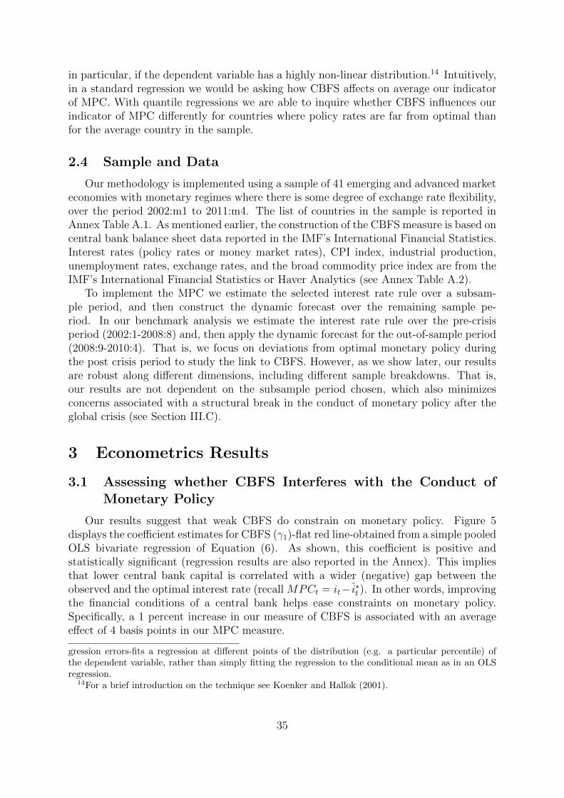
in particular, if the dependent variable has a highly non-linear distribution.14 Intuitively,in a standard regression we would be asking how CBFS affects on average our indicatorof MPC. With quantile regressions we are able to inquire whether CBFS influences ourindicator of MPC differently for countries where policy rates are far from optimal thanfor the average country in the sample.

2.4 Sample and Data

Our methodology is implemented using a sample of 41 emerging and advanced marketeconomies with monetary regimes where there is some degree of exchange rate flexibility,over the period 2002:m1 to 2011:m4. The list of countries in the sample is reported inAnnex Table A.1. As mentioned earlier, the construction of the CBFS measure is based oncentral bank balance sheet data reported in the IMF’s International Financial Statistics.Interest rates (policy rates or money market rates), CPI index, industrial production,unemployment rates, exchange rates, and the broad commodity price index are from theIMF’s International Financial Statistics or Haver Analytics (see Annex Table A.2).

To implement the MPC we estimate the selected interest rate rule over a subsam-ple period, and then construct the dynamic forecast over the remaining sample pe-riod. In our benchmark analysis we estimate the interest rate rule over the pre-crisisperiod (2002:1-2008:8) and, then apply the dynamic forecast for the out-of-sample period(2008:9-2010:4). That is, we focus on deviations from optimal monetary policy duringthe post crisis period to study the link to CBFS. However, as we show later, our resultsare robust along different dimensions, including different sample breakdowns. That is,our results are not dependent on the subsample period chosen, which also minimizesconcerns associated with a structural break in the conduct of monetary policy after theglobal crisis (see Section III.C).

3 Econometrics Results

3.1 Assessing whether CBFS Interferes with the Conduct ofMonetary Policy

Our results suggest that weak CBFS do constrain on monetary policy. Figure 5displays the coefficient estimates for CBFS (γ1)-flat red line-obtained from a simple pooledOLS bivariate regression of Equation (6). As shown, this coefficient is positive andstatistically significant (regression results are also reported in the Annex). This impliesthat lower central bank capital is correlated with a wider (negative) gap between theobserved and the optimal interest rate (recall MPCt = it− i∗t ). In other words, improvingthe financial conditions of a central bank helps ease constraints on monetary policy.Specifically, a 1 percent increase in our measure of CBFS is associated with an averageeffect of 4 basis points in our MPC measure.

gression errors-fits a regression at different points of the distribution (e.g. a particular percentile) ofthe dependent variable, rather than simply fitting the regression to the conditional mean as in an OLSregression.

14For a brief introduction on the technique see Koenker and Hallok (2001).

35

However, we find that the relationship between CBFS and MPC is highly non-linear.Figure 5 also reports the quantile regression estimates with its corresponding 95 percentconfidence interval-blue and gray dotted lines-displaying the impact of CBFS for eachdecile in the distribution of the dependent variable (the MPC indicator). As shown, itis evident that the relationship between CBBS and MPC is non-linear. That is, CBFSappears to play a role when the policy rate is further off from its optimal level. Quan-titatively, this means that, for the first decile of the distribution of MPC (i.e. when theindicator is negative, a 10 percent increase in our CBFS measure decreases the size ofinterest rate gap by 72 basis points (i.e. ∆MPCt = 0.72).15 However, as policy ratesmove closer to their optimal level-i.e. as you move further up in the distribution of thedependent variable- the role of CBBS becomes smaller and mostly statistically irrelevant.This suggests that CBFS plays an important role in cases of large deviations from optimalrates, but less so in cases of small observed deviations.16

Figure 5: Baseline Results from OLS and Quantile Regression

-0.02

0

0.02

0.04

0.06

0.08

0.1

-0.02

0

0.02

0.04

0.06

0.08

0.1

D10 D20 D30 D40 D50 D60 D70 D80 D90

DECILE OLS Quantile Regression

NOTES: Author’s estimates. Horizontal axis: Deciles over the monetary policy constraint (MPC) measure.

Dotted lines show the 95% confidence interval.

Monetary Policy Regime and Development Stage

The importance of CBFS does not vary across monetary regimes. One could thinkof inflation targeting (IT) countries having a more solid framework in place in whichthe strength of the central bank balance sheet at any point in time may not matter, inparticular since the commitment to controlling inflation may be sufficient to ensure thatrecapitalization would take place if required. We explore this by re-estimating the modelonly for IT countries (within EMEs). The estimates for this set of countries (Figure 6)display the same pattern as in the benchmark estimation. That is, CBFS is positivelyrelated with the measure of MPC and non-linearities matter, suggesting that adoption

15Notice that on average the CBFS indicator equals -1.9 in the lowest decile of the reported distributionin Figure 4, while the sample average for the indicator is 5.7.

16Some could argue that there was a structural break in the conduct of monetary policy after Lehmanthat led central banks to set lower interest rates. Therefore large negative MPCs could be the result ofsuch structural break. However, as shown in the regression results (see annex), the relationship remainsstatistically significant even if one moves up in the distribution, that is, for example when the MPC isin the second lowest, third lowest deciles or the median of the regressions (see Figure 6 and Annex withregression results).

36

of an IT regime may not suffice to insulate central bank monetary policy decisions frombalance sheet considerations.

Figure 6: Results for Inflation Targeting Countries



The strength of the general institutional setting does matter. To take this into consid-eration, we explore the sensitivity of our results to a country’s stage of development-usedas a proxy for the strength of the institutional setting-independent of whether an IT ora non-IT regime is in place. For this purpose, the sample is split between developedand developing countries. Interestingly, the baseline results do not hold for developedeconomies, where CBFS appears to have no role even at lower levels Figure 7). This resultshould, however, be interpreted with caution. It can reflect differences in the strength ofthe institutional framework (e.g. central bank independence) but it could also capturethe fact that currency mismatches are normally not present in CBBS of developed coun-tries, and therefore movements in interest rates do not affect significantly central bankcapital.

Figure 7: Results for Developed Countries

-0.02

0

0.02

0.04

0.06

-0.02

0

0.02

0.04

0.06

D10 D20 D30 D40 D50 D60 D70 D80 D90




37

3.2 Robustness Analyses

This section examines the robustness of our results across different critical dimen-sions. Checks include sample variations (both on the time and cross-sectional margins),and adding other controls to the baseline bivariate equation. Notice that unless otherwiseindicated, estimates are all based on our benchmark MPC estimates.

Sample Period Employed for the Estimation of the Interest Rate Rule

We first examine the sensitivity of results to the sample period employed in the esti-mation of the MPC Equation (5). To this end we re-estimate each interest rate rule forthe period 2002-2006:12 and forecast the policy rate over the period 2007:1-2008:12. Inthis manner we aim at assessing whether structural breaks associated with the events thatfollowed the Lehman Brothers’ bankruptcy episode in September 2008 may be influencingour results. OLS and quantile regressions results are qualitatively the same to those ofour benchmark estimates (Figure 8), but there appears to be a level effect. MPCs tend tobe somewhat smaller on average as well as in countries where CBFS is weaker. However,it is worth keeping in mind that a smaller sample size makes our estimates less precise,an effect clearly captured by the wider 95% confidence band.

Figure 8: Results under Alternative Sample Period

-0.02 0 0.02 0.04 0.06 0.08 0.1 0.12

-0.02 0

0.02 0.04 0.06 0.08 0.1

0.12

D10 D20 D30 D40 D50 D60 D70 D80 D90

DECILE

OLS Quantile Regression



In-sample versus out-of-sample forecasts

To further assess whether results may be influenced by recent structural breaks we alsoconstruct a measure of MPC using in-sample (as opposed to out-of-sample) forecasts. Asbefore our measure of monetary policy constraint is the forecast error-but this time this isestimated in-sample. We then use the new forecast errors series to re-estimate Equation(6) over two different sample periods: the whole sample and the period before August2008-i.e. prior to the global crisis (as opposed to the post-August 2008 observations in thebaseline estimation). Both exercises generate the same qualitative results of the baselineestimation (Figures 9 and 10). Quite interesting, these results confirm the importance ofconsidering nonlinearities, which turn out to be somewhat more pronounced than in the

38

Figure 9: Sensitivity to Forecast Sample Period: full sample

-0.02

-0.01

0

0.01

0.02

0.03

0.04

-0.02

-0.01

0

0.01

0.02

0.03

0.04

D10 D20 D30 D40 D50 D60 D70 D80 D90

DECILE




benchmark model.

Figure 10: Sensitivity to Forecast Sample Period: pre 2008:8

-0.02

-0.01

0

0.01

0.02

0.03

0.04

-0.02

-0.01

0

0.01

0.02

0.03

0.04

D10 D20 D30 D40 D50 D60 D70 D80 D90

DECILE




Sensitivity to the CBFS Indicator

How sensitive are the results to the definition of CBFS? As discussed in Section II.A,the accounting entry Other Items Net may include some idiosyncratic features whichmight not be fully comparable across countries. Therefore, we examine the sensitivity ofresults by replacing the baseline definition of CBFS by a simpler ratio, defined as capital-to-total-assets. Our findings indicate that some of the qualitative features do survive,in particular, the non-linearity, but the interpretation is less clear (Figure 11). This isnot surprising because the inclusion of Other Items Net is intended primarily to capturevaluation changes (and reserves) that, even if being one-off items, tend to affect centralbank capital. This confirms, as argued by Ize and Nada (2009), that failing to includesuch valuation changes could invalidate any relationship between capital and financialstrength.

39

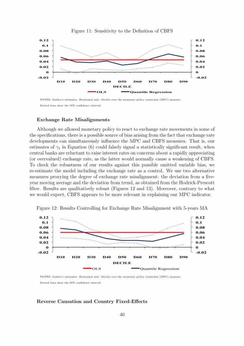
Figure 11: Sensitivity to the Definition of CBFS

-0.02

0

0.02

0.04

0.06

0.08

0.1

0.12

-0.02

0

0.02

0.04

0.06

0.08

0.1

0.12

D10 D20 D30 D40 D50 D60 D70 D80 D90

DECILE




Exchange Rate Misalignments

Although we allowed monetary policy to react to exchange rate movements in some ofthe specifications, there is a possible source of bias arising from the fact that exchange ratedevelopments can simultaneously influence the MPC and CBFS measures. That is, ourestimates of γ1 in Equation (6) could falsely signal a statistically significant result, whencentral banks are reluctant to raise interest rates on concerns about a rapidly appreciating(or overvalued) exchange rate, as the latter would normally cause a weakening of CBFS.To check the robustness of our results against this possible omitted variable bias, were-estimate the model including the exchange rate as a control. We use two alternativemeasures proxying the degree of exchange rate misalignment: the deviation from a five-year moving average and the deviation from trend, as obtained from the Hodrick-Prescottfilter. Results are qualitatively robust (Figures 12 and 13). Moreover, contrary to whatwe would expect, CBFS appears to be more relevant in explaining our MPC indicator.

Figure 12: Results Controlling for Exchange Rate Misalignment with 5-years MA

-0.02 0 0.02 0.04 0.06 0.08 0.1 0.12

-0.02 0

0.02 0.04 0.06 0.08 0.1

0.12

D10 D20 D30 D40 D50 D60 D70 D80 D90

DECILE




Reverse Causation and Country Fixed-Effects

40

Figure 13: Results Controlling for Exchange Rate Misalignment with HP filter

-0.02 0 0.02 0.04 0.06 0.08 0.1 0.12

-0.02 0

0.02 0.04 0.06 0.08

0.1 0.12

D10 D20 D30 D40 D50 D60 D70 D80 D90




Finally, we consider the possibility of endogeneity bias due to reverse causation inEquation (6)-that is, MPC causing CBFS and not the other way round-as well as whethercountry fixed-effects could affect the results. To test for reverse causation, we re-estimateequation (6) using a use a three-month lagged value for CBFS. This choice is motivated onthe basis that we have an autoregressive (AR-2) term in the interest rate rule (Equation(2)). As displayed in Figures 14, the results are qualitatively robust to this change.Quantitatively, both the OLS and quantile regression estimates appear to be slightlysmaller. Similarly, the introduction of country fixed-effects (dummies) does not affect theresults (Figure 15).

Figure 14: Results Controlling for Endogeneity Bias

-0.02 0 0.02 0.04 0.06 0.08 0.1 0.12

-0.02 0

0.02 0.04 0.06 0.08 0.1

0.12

D10 D20 D30 D40 D50 D60 D70 D80 D90

DECILE




Overall, results suggest that CBBS plays a role in constraining monetary policy de-cisions. Moreover, quantile regression estimates show that non-linearities matter: largedeviations from optimal policy are associated with low CBFS.

41

Figure 15: Results Controlling for Country Fixed Effects

-0.06 -0.04 -0.02 0 0.02 0.04 0.06 0.08 0.1

-0.06 -0.04 -0.02

0 0.02 0.04 0.06 0.08

0.1

D10 D20 D30 D40 D50 D60 D70 D80 D90

DECILE




4 Conclusions

Over the past decade, efforts to manage large capital inflows by many central banksacross the emerging market world have led to a major shift in the composition and size oftheir balance sheets. Arguably, such a transformation has made their capital sensitive todomestic interest rate movements, and led to increasing concerns about the implicationsof CBFS for the conduct of monetary policy. Still, research on the importance of centralbank capital for the conduct of monetary policy is quite limited. This paper is, to ourknowledge, the first attempt to conduct a comprehensive analysis of the issue.

We find evidence that a weak central bank balance sheet can influence the conductof monetary policy. Quite importantly, the relationship between central bank balancesheets and monetary policy is highly non-linear-i.e., large deviations from optimal policyare associated with very weak balance sheets. In particular, our estimates suggest thatweak CBBS (of an order of -1.91 in our indicator of CBFS) can lead to a 72 basis pointdeviation of interest rates from its estimated “optimal” level.

Certainly, further research in this area is needed. Future work will need to refine ourmeasure of central bank financial strength and examine alternative indicators to assessthe degree of monetary policy constraint. The former will require a more in depth analysisof CBBS-for which reliance data on a broad basis is still missing-, or the use of explicitmeasures of currency mismatches or interest rate risk in CBBS. Equally important is toimprove our understanding of the specific mechanisms through which CBFS influencesmonetary policy. This includes making a careful assessment of how the macroeconomicand institutional environment, in particular fiscal policies, could influence the outcome.Finally, we also believe that our methodology could also be applied to examine problemsin advanced economies, where CBBS have been expanding rapidly as a result of theadoption of non-traditional policies.

42

A Economic Development and Inflation Targeting

Classification

Table A.1: Economic Development and Inflation Targeting Classification

Inflation Targeting Non Inflation Targeting

Advanced Developing Advanced Developing

Canada Brazil Denmark ArgentinaIceland Chile Japan ChinaIsrael Colombia United States Costa RicaNorway Czech Republic CroatiaSweden Guatemala EgyptSwitzerland Hungary IndiaUnited Kingdom Indonesia Jordan

Korea KazakhstanMexico PakistanPeru RussiaPhilippines TunisiaPoland UruguayRomania VenezuelaSerbiaSouth AfricaThailandTurkey

SOURCE: IMF Classification, Central Banks web sites, and Svensson (2010)

43

B Taylor Rule Variables Definitions

Table A.2: Taylor Rule Variables Definition

Variable Definition

Interest Rate Policy rate or money market rate

12-month InflationDifference of log Consumer Price Inflation index inthe current month and its value 12 months before,multiplied by 100

Industrial Production Log of Industrial Production Index

Industrial Production GapDifference between Industrial Production and itstrend value, multiplied by 100

Industrial Production Gap 3-month ahead

Sum of industrial production gap in the next threemonths

Unemployment Rate GapDifference between unemployment rate and itstrend value, multiplied by -1

Unemployment Gap 3-monthahead

Sum of unemployment gap in the next threemonths

Exchange Rate DepreciationDifference between log U.S. dollar nominal ex-change rate in two consecutive months, multipliedby 100

Exchange Rate Depreciation inthe Last 3-months

Sum of Exchange Rate Depreciation in the lastthree months

C Main Regression Tables

Table A.3: Benchmark: Pooled OLS Regression

Variables Coefficients

CBFS0.0414***(0.0091)

Constant-1.520***(0.1660)

Observations 813R-squared 0.032

NOTES: Robust Standard Errors in Parentheses; *** stands for 1% significance level

44

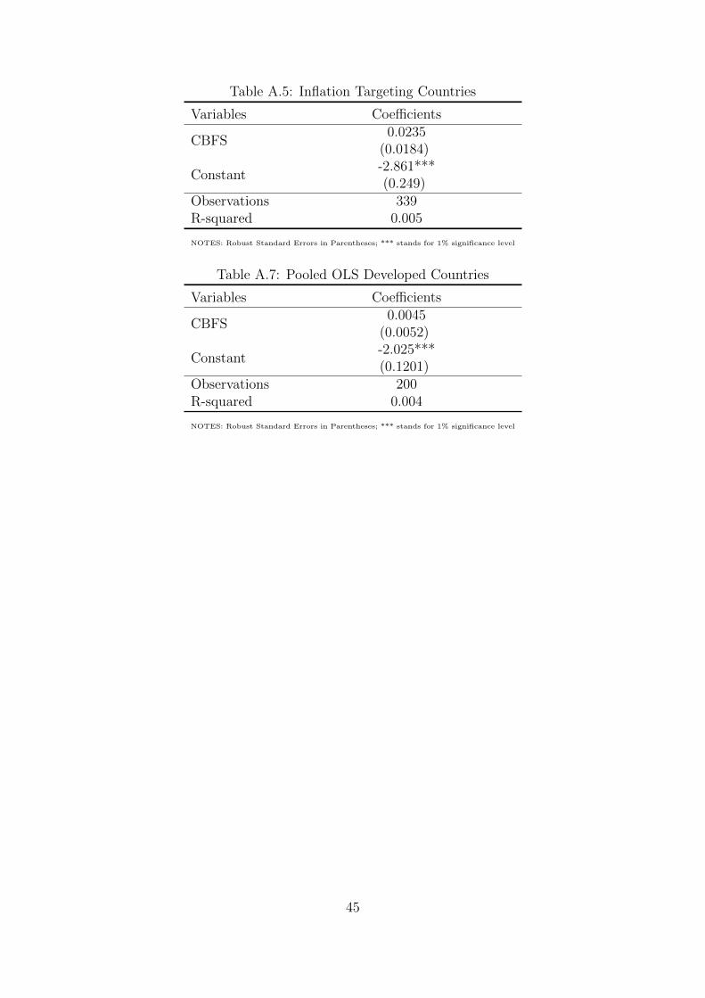
Table A.5: Inflation Targeting Countries


CBFS0.0235

(0.0184)

Constant-2.861***(0.249)



Table A.7: Pooled OLS Developed Countries


CBFS0.0045

(0.0052)

Constant-2.025***(0.1201)



45

References

[1] Adler, Gustavo and Camilo Tovar, “Foreign Exchange Intervention: A Shield againstAppreciation Winds?,” International Monetary Fund, Working Paper 11/165, Wash-ington, 2011.

[2] Benecka, Sona, Tomas Holhub, Narcisa Liliana Kadlcakova, and Ivana Kubikova,“Central Bank Financial Strength and Inflation: Is There an Empirical Link?,” CzechRepublic Central Bank, Mimeo, 2-12.

[3] Clarida, Richard, Jordi Galim and Mark Gertler, “Monetary Policy Rules and Macroe-conomic Stability: Evidence and Some Theory,” Quarterly Journal of Economics, p.147-180, February 2000.

[4] Clarida, Richard, Jordi Gali and Mark Gertler, “Monetary Policy Rules in Practice:Some International Evidence,” European Economic Review,42, p. 1033-1067, 1998.

[5] Clark, Todd and Kenneth West, “Using Out-of-Sample Mean Squared PredictionErrors to Test the Martingale Difference Hypothesis,” Journal of Econometrics, 135,p. 155-186, 2006.

[6] Clark, Todd and Kenneth West, “Approximately Normal Tests for Equal PredictiveAccuracy in Nested Models,” Journal of Econometrics, 138, p. 291-311, 2006.

[7] Ize, Alain, “Capitalizing Central Banks: a Net Worth Approach,” International Mon-etary Fund, Working Paper 05/15, Washington, 2005.

[8] Ize, Alain and Nada Oulidi, “Why do Central Banks Go Weak?,” International Mon-etary Fund, Working Paper 09/13, Washington, 2009.

[9] Jeanne, Olivier and Lars Svensson, “Credible Commitment to Optimal Escape fromLiquidity Trap: The Role of Balance Sheet of an Independent Central Bank,” Amer-ican Economic Review, 97 (1), p.474-490, 2007.

[10] Kluh, Ulrich and Peter Stella, “Central Bank Financial Strength and Policy Perfor-mance: an Econometric Evaluation,” International Monetary Fund, Working Paper08/17, Washington, 2008.

[11] Koenker, Roger and Kevin Hallok, “Quantile Regression,” Journal of EconometricPerspectives, 15 (4), p.143-156, 2001.

[12] Lonnberg, Ake, and Peter Stella “Issues in Central Bank Finance Independence,”Federal Reserve Bank of Atlanta, N. 13, Atlanta, 2008.

[13] Moura, Marcelo and Alexandre Carvalho, “What Can Taylor Rules Say About Mon-etary Policy in Latin America?,” Journal of Macroeconomics, 32, p. 292-404, 2010.

[14] Nelson, Mark, “Exchange Rate and Fundamentals: Evidence on Long-Horizon Pre-dictability,” American Economic Review, 85 (1), p.201-218, 1995.

46

[15] Restrepo, Jorge, Luis Salomo, and Rodrigo Valdes, “Macroeconomia, Politica Mon-etaria y Patrimonio del Banco Central de Chile,” Economia Chilena, 12 (1), 2009.

[16] Sims, Christopher, “Fiscal Aspects of Central Bank Independence,” CESifn WorkingPaper 547, August 2001.

[17] Sims, Christopher, “Limits to Inflation Targeting,” in: The Inflation-Targeting De-bate, ed. by Ben Bernanke and Michael Woodford, University of Chicago Press,Chicago, 2004.

[18] Stella, Peter, “Do Central Banks Need Capital?,” International Monetary Fund,Working Paper 97/83, Washington, 1997.

[19] Stella, Peter, “Central Bank Financial Strength, Transparency and Policy Credibil-ity,” International Monetary Fund Staff Papers, 52 (2), p.335-365, 2005.

[20] Taylor, John, “Discretion versus Policy Rules in Practice,” Carnegie-Rochester Con-ference Series on Public Policies, 39, p.194-214, North Holland, 1993.

47

Chapter 03The Role of the Exchange Rate in Inflation Targeting

Regimes∗

Abstract

My goal is to assess how Inflation Targeting (henceforth, IT) countries conduct mon-etary policy and, in particular, how policymakers have reacted to exchange rate move-ments. I present stylized facts which suggest that exchange rates have been allowed tofloat relatively free in IT countries. I employ Bayesian Analysis techniques to estimatea Dynamic Stochastic General Equilibrium (DSGE) structural model for twenty two ITeconomies and compute posterior odds tests to check whether the central banks system-atically respond to exchange rate movements. The main result is that only five centralbanks directly respond to exchange rate movements; all the other IT central banks do notrespond to the exchange rate. I also confirm that IT central banks have been conductingstrictly inflationary policies, raising real interest rates in response to increases in inflation.

∗Department of Economics, University of California, Berkeley. I am grateful to Maurice Obstfeldfor his support throughout my research. Barry Eichengreen, Pierre-Olivier Gourinchas, Yuriy Gorod-nichenko, Andrew Rose, David Romer, Demian Pouzo, Brad DeLong, and seminar participants at UCBerkeley provided valuable feedback. All errors are my own.

48

1 Introduction

Despite being a relatively new approach to monetary policy the inflation targeting(henceforth, IT) framework is now fully implemented in twenty seven countries aroundthe world. The framework is known for the public announcement of numerical values ofan inflation target and the subordination of all other policy objectives to its achievement.1

The empirical evidence regarding its success is often positive and there is no evidencethat it was harmful for its adopters. Also, its durability and the fact that it has beenexpanding without any coordination led some to emphasize its relevance in shaping anew international monetary system.2

This paper aims to understand the role of the exchange rate in the IT regimes. ITrequires nominal exchange rate flexibility; in an economy with unrestricted capital flows,if the monetary policy is focused on domestic conditions the nominal exchange rate mustbe allowed to fluctuate. Despite this seemly simple requirement, discussions about theappropriate level and flexibility of the exchange rate are still central in the policy debateof IT economies and economists often disagree on the degree to which IT central banksactually respond to exchange rate movements. This paper contributes to this debatein two ways. First, I present several stylized facts showing that exchange rates havebeen floating relatively free in IT economies; whether I compare the exchange rates of ITeconomies with those of non-IT ones or with their own exchange rates before the adoptionof the framework the result is always that the adoption of IT is associated with greaterexchange rate flexibility. I also show that interest rates in IT economies have showedlower variability than in non-IT ones. Second, I estimate a structural model and payspecial attention to policy responses to exchange rate movements. I find that most ITcentral banks do not directly respond to exchange rate movements, and confirm the factthat they have been conducting strictly anti-inflationary policies as stated by the TaylorPrinciple.

From a perspective of an optimal response to inflation deviations from the target theliterature does not offer a definitive answer to whether an IT central bank should respondto exchange rate movements. The literature in this area has advanced both with theoret-ical models and empirical exercises. Svensson (2000) develops and simulates a small openeconomy model and suggests that policymakers should directly respond to exchange ratemovements. Svensson claims that by responding to the exchange rate the IT central bankcan affect domestic inflation with a shorter lag and be more effective in anchoring infla-tion expectations. On the other hand, Taylor (2001) suggests that, although it is possibleto achieve better outcomes by making interest rates respond to exchange rate changes,the gains are often small and it may actually lead to worse outcomes, adding unneces-sary variability to interest rates and output.3 In a case study Jonas and Mishkin (2005)

1The other defining elements of IT enumerated by Mishkin (2002) are: an information inclusivestrategy in which all relevant information is used for taking policy decisions; increased transparencyof monetary policy by extended communication with the public aiming to make clear the reasoningbehind the policy plans, objectives and decisions; and increased accountability of the central bank forits achievements regarding the inflation target.

2In this regard see Rose (2007).3Taylor stresses that a monetary authority who follows a policy rule without an explicit reaction to

the exchange rate already responds to its changes indirectly, as exchange rate changes will eventuallyimpact the output and inflation. Also, directly reacting to exchange rate movements can add undesirable

49

analyzed the IT experiences of Eastern Europe economies; they argue that automaticresponses to the exchanges rate movements are not desirable and that more attentionshould be given to the source of the underlying shock.4 Another case study by Bernankeet al. (1999) suggests that IT central banks have different views on how recent devel-opments of the exchange rate should be incorporated in the decision making processes,but explicitly managing the exchange rate have become increasingly uncommon despitecentral banks often showing reluctance to allow the exchange rate to free float.5

The adoption of the IT framework among emerging markets and transition economiesled some economists to question if these countries were apt to deal with the amountof exchange rate flexibility that IT requires. In these economies the exchange rate hasbeen in the very center of the policy debate for decades. Historically many of them usedthe exchange rate with multiple policy objectives, such as promoting industrializationor generating fiscal revenues by implicitly taxing exports. More recently, exchange ratepegs were implemented in stabilization plans which allowed them to bring down inflation;however, this experience tended to end with exchange rate overvaluation and currencycrises. The IT framework was then adopted with the goal to preserve the gains from lowinflation while avoiding the crises that forced the abandonment of the peg arrangements.

Lack of monetary policy credibility and high-pass through of exchange rate movementsto domestic prices rendered the IT implementation especially challenging in emergingmarkets. In a much debated paper, Calvo and Reinhart (2002) suggest that countriesthat claim to allow their exchange rate to fluctuate actually do not; they have “fearof floating”. They suggest that “fear of floating” is caused by high pass-through fromexchange rate movements to domestic prices, lack of monetary policy credibility andaggressive responses to inflation deviations from the target. The results in this papershow that there is more heterogeneity in exchange rate regimes than the “fear of floating”concept suggests.6 In particular, the countries that adopted IT have been notably willingto allow their exchange rates to float. Although “fear of floating” might be justifiable, thispaper shows that the greater degree of exchange rate flexibility verified in IT countriesis a consequence of policy choices, given that for most of IT countries interest rates havebeen set without any direct response to exchange rate movements.

Another important challenge associated with the IT implementation is that exchangerate movements can generate negative balance sheet effects for countries with foreigncurrency denominated debt. Eichengreen and Hausmann (1999) document that only few

volatility to monetary policy if these movements represent departures from purchasing power parity(PPP); in this regard see also Obstfeld and Rogoff (1995b) and Edwards (2006).

4Jonas and Mishkin suggest that the lack of attention to the source of exchange rate movements duringEast Asia 1997 crises led New Zealand and Chile to raise interest rates, “a serious policy mistake”, whileAustralian policymakers recognized that the large negative terms of trade shock called for loweringinterest rates despite the large depreciation of the currency.

5For example, Bernanke et al. describe the tensions that led New Zealand and Canada to use amonetary conditions index (MCI) “as a means to assess the overall stance of monetary policy”. Incontrast, Australia tends to pay relatively less attention to the behavior of exchange rates and Israel“gradually de-emphasized strict bands for the exchange rate in favor of a policy that responds to exchangerate changes only when they are deemed likely to affect domestic prices.”

6The “fear of floating” suggests a convergence of the de-facto exchange rate regimes, with the countriespracticing some form of crawling peg or managed floating with little difference among them in practice;in the other extreme of the literature is the “bipolar” view, according to which exchange rate regimeshave been moving toward free floating or hard currency pegs.

50

countries are able to borrow abroad in domestic currency. According to the “originalsin” view all the other countries have no other option but to borrow in foreign currency,making the real size of their debt contingent on the value of the exchange rate and in-creasing the likelihood of self-fulfilling crisis.7 If a significant amount of public debt isdenominated in foreign currency a depreciation of the domestic currency can dramati-cally increase the size of the public debt, leading to “fiscal dominance” and forcing theabandonment of the inflation target.8 When the financial sector has foreign currencydenominated liabilities, an exchange rate depreciation can lead to bank runs and capitaloutflows, exacerbating the depreciation of the currency and rendering the target infeasi-ble. If the private non-financial sector debt increases with exchange rate depreciations, itsinvestment capacity might become compromised generating prolonged recessions and/orit might have to default on its debt, possibly generating perverse feedbacks to the finan-cial sector. This paper shows that most of IT economies have managed to focus monetarypolicy on domestic objectives, namely inflation and output levels, without setting interestrates to influence the level of the exchange rate. The result of this paper showing that ITeconomies have not experienced “fear of floating”, with the exchange rate being allowedto play its role as an external adjustment mechanism, gains especial relevance when oneconsiders the rapid growth of gross global financial positions across the world and theincreasing relevance of IT for the international monetary system.9

Finally, this paper also has implications for the currency crises literature. Caballeroand Krishnamurthy (2005) show that the response of IT central banks to exchange ratemovements has important implications to the private sector incentives to hedge its bal-ance sheet against episodes of large depreciations. In particular, they show that althoughit is optimal for an IT central bank to prevent large depreciations ex-post, the centralbank can achieve a welfare superior outcome if it commits ex-ante to allow the currencyto depreciate. Knowing this commitment, agents would hedge their foreign denominatedliabilities, reducing the disruption generated by sudden stops. My research shows thatIT central banks have indeed allowed the exchange rate to fluctuate and, although inves-tigating the implications of this behavior to the accumulation of currency mismatches isbeyond the scope of this chapter, the fact that IT experiences have been long lasting sug-gest that these economies have avoided the build up of imbalances that lead to currencycrises.

The chapter is structured as follows. In section two I present stylized facts showingthat exchange rate flexibility has been particularly high in IT countries. In section threeI discuss the decision to adopt IT. In section four I describe the data. In section five Idescribe the structural model estimated, the technique used for its estimation and theresults. Section six concludes.

7For a case study on the relationship between currency crisis and foreign currency debt see Diaz-Alejandro (1983). For a seminal paper on the self fulfilling nature of currency crises see Obstfeld (1994).

8For more on “fiscal dominance” see Blanchard (2004) and Sims (2005)9The build up of gross global financial positions is documented in Obstfeld (2012).

51

2 Exchange Rate Volatility in IT Regimes

2.1 Frequency Analyses

One of the main criticisms regarding IT is that the exchange rate volatility that itrequires to function may outweigh the benefits of focusing monetary policy on domesticconditions. When a country faces a shock which causes exchange rate depreciation,the pass-through of higher import prices into domestic prices and the effect of termsof trade changes into domestic output may require that the central bank responds bychanging the interest rate. The critics argue that, since the exchange rate movementswill generally affect domestic conditions faster than changes in the interest rate, IT canlead to excessive output and interest rate variability, and IT central banks will end upbeing forced to prevent the exchange rate from fluctuating.

However, it is not clear that this should be the case. One possibility is that the lowerinflation environment and higher policy credibility which the IT framework generateswill actually reduce the degree of pass-through from exchange rate to prices. In thiscase central banks would not respond aggressively to exchange rate movements, and theoutput and interest rate volatility may not increase.

Therefore, it is important to know how the exchange rate volatility in IT economiescompare to that in non-IT ones. There seems to be little consensus about this. Asmentioned above, some critics suggest that one of the main costs of IT is associated withhigher exchange rate volatility. However, in an influential paper Calvo and Reinhart(2002) showed that countries which announce floating exchange rate regimes actually donot allow their currencies to float; they have “fear of floating”. They present a simplemodel where an IT central bank will display such behavior due to high pass-through andan aggressive response to deviations of inflation from the target.

In this Section I present stylized facts showing that exchange rates have been fluctu-ating relatively free in IT economies and that there is no evidence that interest rates andreserves have been used to stabilize the value of the currency.

In Table 1 I use an empirical approach similar to Calvo and Reinhart (2002) in orderto investigate if exchange rates have been allowed to float in IT countries. For thispurpose I divide the sample of 54 countries into two groups: 27 IT countries and 27non-IT countries. I also present individual statistics for the US, Japan and Australia.

The exercise focuses on the analysis of four variables: the absolute value of the per-centage changes of dollar exchange rate |∆e|

e, the absolute value of the percentage changes

of the real exchange rate |∆λ|λ

, the absolute value of the percentage changes of the foreign

reserves-M2 ratio |∆H|H

and the absolute value of the change of the nominal interest rate|∆R|.10 Denoting by t the value of some threshold, I calculate the probability that thevariable of interest is smaller than this threshold in the sample period; for example, theprobability that the absolute value of dollar exchange rate changes is lower than two anda half percent, that is, Pr( |∆e|

e< 0.025). The prediction is that countries which allow

their currencies to float will have a higher frequency of large changes in the exchangerates and a lower frequency of large changes in foreign reserves and interest rates. Table1 also shows in parenthesis the standard deviation of the four variables analyzed.

10I also did the same exercises using the absolute value of percentage changes of the foreign reserves;the results were essentially the same and are available upon request.

52

The statistics for the IT group and Australia (which is itself an IT country) are com-puted using data since adoption of IT (the specific dates can be found in the Appendix);for the non-IT countries the results were calculated from July 1999 (the average date ofimplementation of IT regimes) to March 2011. The statistics for the absolute value ofthe percentage change of the dollar and real exchange rates and foreign reserves - M2ratio are relative to a two and half percent threshold and for the change in the nominalinterest rates are relative to a half percent (or fifty basis points) threshold.

The statistics presented in the Table 1 show that exchange rates have been floatingin IT regimes. The likelihood of large percentage changes of the dollar and the realexchange rates is always larger for IT economies in comparison to non-IT ones, evenwhen I consider IT developed economies and IT emerging markets separately. In par-ticular, the exchange rate of IT emerging markets are among the ones which fluctuatethe most. Large changes in foreign reserves and interest rates are more likely in non-ITeconomies, suggesting that IT economies have not been using these instruments to man-age the exchange rate. Perhaps surprisingly, the reserves of IT emerging markets havelarge changes less frequently than in IT developed economies. It is also notable that largeinterest rate movements occurs as frequently in IT emerging markets and as in IT devel-oped economies. The same results are obtained when I analyze the standard deviation ofthese variables. The standard deviations of the dollar and real exchange rates are high inIT economies when compared to non-IT ones (this is particularly true for emerging mar-kets) and the instruments used to influence the exchange rate, interest rate and foreignreserves, have lower standard deviations in IT economies, showing that IT central bankshave not systematically tried to prevent the exchange rate from fluctuating.

Table 1: Frequency Analyses (Post IT Period)

Country/GroupsProbabilities and Standard Errors

|∆e|e < 2.5% |∆λ|

λ < 2.5% |∆H|H < 2.5% |∆R| < 0.5%

IT average0.71

(1.67)0.82

(1.37)0.52

(1.34)0.82

(0.46)

IT emergingmarkets

0.68(1.76)

0.78(1.50)

0.58(1.32)

0.82(0.51)

IT developedcountries

0.74(1.57)

0.84(1.18)

0.44(1.36)

0.83(0.39)

non-IT0.87

(1.38)0.90

(1.23)0.48

(1.35)0.69

(0.83)

Australia0.66

(1.58)0.78

(1.30)0.36

(1.37)0.96

(0.17)

United States0.92

(0.91)0.94

(0.88)0.70

(1.17)0.95

(0.17)

Japan0.72

(1.47)0.77

(1.59)0.84

(0.95)1.00

(0.03)

NOTE: Author’s calculations. Standard errors in parenthesis.

The fact that exchange rates have been fluctuating in IT economies is apparent whenI use other approaches to analyze the data. Figure 1 below shows the distribution of

53

exchange rates percentage changes. In the top two graphs I compare the movements ofthe dollar and the real exchange rates in IT and non-IT economies; at top left, the twogroups’ real exchange rate percentage change distributions are plotted while, at top right,the same thing is done but now using the dollar exchange rate.

The bottom graphs of Figure 1 compare the distribution of monthly exchange ratepercentage changes in IT economies before and after the adoption of the framework. Thebottom-left graph shows the distributions of percentage changes in the real exchange ratebefore and after IT adoption, while the bottom-right graph does the same for the dollarexchange rate. The graphs in Figure 1 show that the exchange rate fluctuates more inIT than in non-IT economies; they also show that the exchange rate has been fluctuatingmore in IT economies since the framework was adopted. Overall, IT regimes have beencharacterized by a great degree of exchange rate flexibility.

Formal statistical tests reject the null hypothesis of equality of distribution and vari-ance in all the cases analyzed in Figure 1. The null hypothesis is always rejected at the5% significance level (Table 2).

Table 2: Tests of Equality of Distribution and Variance

Groups Compared ER DefinitionReject EqualDistribution?

Reject EqualVariance?

IT and non-ITDollar ER Yes*** Yes***Real ER Yes*** Yes***

IT: before and afterDollar ER Yes*** Yes***Real ER Yes*** Yes**

NOTE: *** and ** stand for 1% and 5% rejection levels, respectively.

Finally, I check whether the results of the comparison between the IT and non-ITeconomies are driven by outliers from one group or the other. The table below shows howmany IT and non-IT economies are in each quartile of the distribution of the countries’(dollar and real) exchange rate percentage changes variances for the period after ITadoption (and after July 1999 for non-IT economies). The main conclusion is that non-IT economies do have lower exchange rate change variances as they are overrepresentedin the lower quartiles of the distribution of both the dollar and the real exchange ratechanges.

Table 3: Distribution of Exchange Rate Change Variance by CountryReal Exchange Rate Percentage Change Variance

Quartile 1 Quartile 2 Quartile 3 Quartile 4 Total

IT 3 7 7 7 24

Non-IT 9 5 5 4 23

Dollar Exchange Rate Percentage Change VarianceQuartile 1 Quartile 2 Quartile 3 Quartile 4 Total

IT 3 5 10 9 27

Non-IT 10 8 3 6 27

NOTES: Author’s calculations. Quartile 1 corresponds to the 25% of countries with lowest variances and Quartile 4 to the 25% of

countries with highest variances of exchange rate percentage changes.

54

Figure 1: Real and Nominal Exchange Rate Depreciation Densities: IT and non-IT0

.1.2

.3.4

Density


IT nonIT

Kernel densities IT and non IT countries

0.2

.4.6

.8D

ensity


IT nonIT

Kernel densities: IT and non IT countries0

.1.2

.3D

ensity


After IT Before IT


0.1

.2.3

.4D

ensity


After IT Before IT


3 Why Adopt IT?

An important question is why countries adopt IT. In this section I briefly make someconsiderations regarding this decision.

Inflation Targeting is generally viewed as a way to bolster the credibility of mone-tary policy. Its emphasis on communication is seen as anchoring expectations of futureinflation, possibly leading to a more favorable inflation output trade-off.

Bernanke et al. (1999) defines IT as:“...a framework for monetary policy characterized by the public announcement of of-

ficial quantitative targets (or target ranges) for the inflation rate over one or more targethorizons, and by explicit acknowledgement that low, stable inflation is monetary policy’s

55

primary long-run goal.”IT is therefore a framework that assigns monetary policy decisions to domestic goals.

An important condition for making domestic inflation the main policy target is to allowfor some degree of exchange rate fluctuation. With open capital accounts, monetarypolicy cannot be focused on domestic objectives unless the value of the currency canchange. This is known as the open economy trilemma.11 In the other extreme, somecountries choose to peg their currencies or to keep tight controls of capital flows. Asmall open economy closely related to a larger one will have greater benefits by fixing itsexchange rate relative to that larger economy’s currency. Also an economy with closedcapital account will not have much to gain from an IT regime, given that it can controldomestic interest rates and the exchange rate simultaneously.

One of the main costs of IT is the requirement of a floating exchange rate regime.Exchange rate volatility tends to generate inflation shocks (in the form of pass-throughof imports prices to domestic prices) and terms of trade shocks which may require tightermonetary policy and induce higher output volatility. Some economists have suggestedthat IT has reduced the costs associated with flexible exchange rates; Bernanke et al.suggests that it has generated an environment of “constrained discretion” for monetarypolicy, combining the benefits of rules and discretion. The benefits generally associatedwith IT include the achievement of lower inflation rates and inflation expectations, lowerpass-through into inflation of exchange rate shocks, insulation of policymakers from po-litical pressures, and greater policymaker accountability.

4 Data

All the data used in this paper were obtained in the International Financial Statistics(IFS/IMF) database.

All variables analyzed in Section 2 above have monthly frequency. The dollar exchangerate is always the nominal exchange rate relative to the US dollar and is given by thenominal “market rate” concept in the IFS data set. The real exchange rate is the consumerprice index (CPI) based real exchange rate (“rec” concept). The reserves are given bythe variable “total reserves minus gold” in the IFS data. The interest rate definition usedis the “money market” interest rate.

In Section 5 below I estimate a structural model (described below) for twenty two ITeconomies. These countries were selected because they have a long enough experiencewith the IT framework that allowed me to estimate the model. The data used haveobservations for the real output growth, inflation, nominal interest rates, nominal effectiveexchange rate changes, and terms of trade changes. The structural model was estimatedusing quarterly frequency data. The data for each country start in the quarter when ITwas adopted and the last observation is always for the 2011:1 quarter.

All data in Section 5 are seasonally adjusted. The output growth rate is the log dif-ference of real GDP, which was multiplied by 100 to obtain quarter-to-quarter percentagegrowth rates. The inflation rate used is the log difference of the CPI index, multipliedby 400 to obtain annualized rates. The nominal interest rates correspond to the average

11For a detailed discussion on the monetary policy trilemma see Obstfeld et al. (2005) and Obstfeldet al. (2010).

56

target rate specified by each central bank in a given quarter. The exchange rate changecorresponds to the log difference, multiplied by 100, of the average nominal effectiveexchange rate in a given quarter (positive changes correspond to a depreciation). Theterms of trade data were converted into log differences and then multiplied by 100 inorder to obtain quarter-to-quarter percentage changes. All series were demeaned prior tothe structural model estimation.

5 Structural Model

5.1 Model Description

In this section I estimate a dynamic stochastic general equilibrium (DSGE) model fortwenty two IT countries.12 The model fitted represents a small open economy close tothat in Gali and Monacelli (2005) which follows the tradition of the New Open EconomyMacroeconomics (NOEM) models. The empirical technique, Bayesian analysis, is basedon Lubik and Schorfheide (2007).

Until recently, the most common strategy adopted by economists who sought to in-vestigate whether central banks respond to exchange rate movements was to estimatea Taylor rule expanded to allow for an exchange response, an approach that becamepopular after the work of Clarida, Gali and Gertler (1998). The reduced form approachwas used, for example, by Eichengreen (2004), who investigated if the Bank of Korearesponded to the exchange rate in the period from 1998 to 2003.

The structural approach allows the econometrician to avoid the problems related toendogenous independent variables that have been in the center of the criticism to reducedform estimates since it incorporates the model structural restrictions in the estimation.One advantage of the Bayesian estimation procedure is that additional information maybe added to the estimation when assigning prior distributions to the parameters. More-over, the estimates allow the evaluation of the importance of different structural shocksthrough impulse response functions and variance decompositions.13

The Bayesian estimation procedure involves the specification of a prior distributionfor the parameters θ to be estimated, f (θ). The data is then used to construct a like-lihood function associated with the model economy, L (θ|YT ); where YT = [Y1, ..., YT ] isa matrix where each column is a vector composed of the observable variables in periodt, Yt. Finally, the Bayes Theorem is used to determine the posterior distribution of theparameters:

f (θ|YT ) = L(θ|YT )f(θ)∫L(θ|YT )f(θ)d(θ)

The model is an open economy extension of the New Keynesian model first developedfor closed economies. As in its closed economy counterpart the model consists of an ISequation and a Phillips curve, but here expanded to take into account the interaction be-tween the domestic economy and the rest of the world. The exchange rate is introduced

12I estimate the model for twenty two IT countries, instead of doing it for all the twenty seven, becausesome them adopted the framework recently making the available series too short for the estimation ofthe model.

13For an introduction to the Bayesian analysis of DSGE models see An and Schorfheide (2005).

57

in the definition of the consumer price index (CPI) and the terms of trade is governed byan exogenous AR(1) process. Finally, the model is closed with an interest rate relation-ship as in Taylor (1993) expanded to allow for interest smoothing and for policymakers’response to the exchange rate movements.

The open-economy IS equation is obtained by combining the consumption Euler equa-tion, the goods market clearing condition and the assumption of complete securities mar-ket:

yt = Etyt+1−[τ + α (2− α) (1− τ)] (rt − Etπt+1)−ρzzt−α [τ + α (2− α) (1− τ)]Et∆qt+1+α (2− α)

(1−ττ

)Et∆y

∗t+1

where (1− α) is related to the degree of home bias in preferences, (α can be inter-preted as openness measure), τ is the elasticity of intertemporal substitution, y∗ is theexogenous world output, z is the world productivity growth rate, and qt is the terms oftrade. The endogenous variables are the aggregate output yt and the CPI inflation rateπt. The world productivity level evolves according to:

AtAt−1

= γezt

where zt = ρzZt−1 +εzt . The Phillips curve is derived from the firms’ optimal strategyin a Calvo price setting:

πt = βEtπt+1 + αβEt∆qt+1 + κτ+α(2−α)(1−τ)

(yt − yt)

Where yt = −α (2− α) (1− τ) 1τy∗t

is the potential output, the slope of the Phillips

curve κ is a function of different structural parameters and β is the discount rate.I now go over the main steps of the derivation of an equation linking movements in

the consumer price index (CPI), the nominal exchange rate, the terms of trade and theworld price index. The log-linearized CPI equation is given by:

pt = (1− α) pH,t + αpF,t

pt = pH,t − αqt

where pt is the log of the CPI index, pF,t is the log of the price index of the importedgoods, pH,t is the log of the price index for the domestically produced goods, and qt =pH,t − pF,t is the (log) terms of trade.

It is possible to obtain an expression linking the (log) price index of imported goods,pF,t, the (log) nominal effective exchange rate, et, and the (log) world price index, p∗t :

pF,t = et + p∗t

Then, using the definitions of the terms of trade and of the CPI index, it turns outthat the CPI inflation can be described as a function of the exchange rate depreciation∆et, the terms of trade change ∆qt and the rest of the world inflation π∗t :

58

πt = ∆et + (1− α) ∆qt + π∗t

The terms of trade growth rate is assumed to evolve according to an exogenous AR(1)process:

∆qt = ρq∆qt−1 + εqt

The interest rate rule allows for the possibility that policymakers respond to exchangerate devaluations (i.e., ψ3 6= 0):

rt = ρrrt−1 + (1− ρr) [ψ1πt + ψ2yt + ψ3et] + εrt

Where rt is the interest rate, ρr is a smoothing term included to match the persistenceof nominal interest rates and εrt is a white noise policy shock. Finally, the world outputand inflation are both assumed to follow autoregressive processes:

π∗t = ρπ∗π∗t−1 + επ

∗t

y∗t = ρy∗y∗t−1 + εy

∗

t

The Bayesian estimation method provides a straightforward way to answer the ques-tion of how the central banks react to exchange rate movements. In order to do this twoversions of the model are estimated; one imposes ψ3 > 0 (model A) and the other ψ3 = 0(model B). The posterior odds ratio of the two model specifications is then calculated andit is the statistic used to judge which model fits the data better. Formally, the posteriorodds ratio is given by:

πA,TπB,T

=πA,0πB,0

pr(Y T |A)pr(Y T |B)

The first factor is the prior odds ratio in favor of model A. The second factor is knownas the Bayes factor and corresponds to the sample evidence in favor of model A. The termpr

(Y T |A

)is the marginal data density. I impose a prior odds ratio equal to one.

5.2 Estimation

I follow Lubik and Schorfheide (2007) to choose the structural parameters priors. Ispecify prior distributions for each parameter and assume they are independently dis-tributed. The complete description of the priors is in Table 3.

The prior distributions of the Taylor rule parameters (Table 3) are centered at valuescommonly found in the literature and allows for a fair amount of parameter uncertainty.The interest rate smoothing coefficient prior has mean 0.50 and standard deviation 0.20.The prior distribution of the steady state interest rate has mean 2.5% and standarddeviation 1.00. The slope of the Phillips curve coefficient has mean 0.50 with a relativelylarge standard deviation. The prior for the preference parameter α has mean 0.20 andstandard deviation 0.05. The parameter τ is restricted to be smaller than one, with amean of 0.50. Finally, the priors of autoregressive coefficients of the foreign inflation, rest

59

of the world output, technology growth and terms of trade growth are centered at 0.80,0.90, 0.40 and 0.20, respectively. I choose identical parameters for each model economy.

The policy rule estimated parameters are in line with results previously found in theliterature (Table 4). The estimates show that all central banks pursue anti-inflationarypolicies; with the response to inflation coefficients ranging from 1.08 to 2.82 (UnitedKingdom and New Zealand, respectively). The response to the output is the highest inSouth Africa (ψ2 = 0.44) and the lowest in Korea and Thailand (ψ2 = 0.04). There isalso a high degree of interest rate smoothing, with all estimates of ρr above 0.60. Finally,among the economies for which I found evidence of a policy response to exchange ratemovements (see Table 5 below), the response is the highest in Israel ψ3 = 0.43 and thelowest in New Zealand ψ3 = 0.13. It is noteworthy that the parameters estimates fall ina relatively wide range, giving no indication that the prior distributions imposed severerestrictions to the posterior mean.

A question that the literature on monetary policy has been concerned with is whetherthe coefficients of the Taylor rule are such that determinacy of the equilibrium is ensured.Woodford (2003) shows that, for different classes of models, the determinacy of the equi-librium is ensured for coefficients of inflation and output with magnitudes equal to thosepresented in Table 4.14

Table 3: Prior Distribution of Parameters

Parameter Distribution Mean*Standard

Deviation*Domain

ψ1 Gamma 1.5 0.5 [0,∞)

ψ2 Gamma 0.25 0.13 [0,∞)

ψ3 Gamma 0.25 0.13 [0,∞)

ρr Beta 0.50 0.2 [0, 1)

ρq Beta 0.20 0.10 [0, 1)

ρz Beta 0.40 0.10 [0, 1)

ρy∗ Beta 0.90 0.05 [0, 1)

ρπ∗ Beta 0.80 0.10 [0, 1)

α Beta 0.20 0.05 [0, 1)

rr Gamma 2.50 1.00 [0,∞)

κ Gamma 0.50 0.25 [0,∞)

τ Beta 0.50 0.20 [0, 1)

σr Inv. Gamma 0.50 4.00 [0,∞)

σq Inv. Gamma 1.50 4.00 [0,∞)

σz Inv. Gamma 1.00 4.00 [0,∞)

σy∗ Inv. Gamma 1.50 4.00 [0,∞)

σπ∗ Inv. Gamma 0.55 4.00 [0,∞)

*NOTE: For the inverse gamma p.d.f. the values in the mean and standard deviation columns stand for, respectively, the

parameters s and v in p (σ|v, s) ∝ σ−v−1e−vs22σ2

14See Woodford (2003) chapter 4; in particular, pages 252 to 261.

60

Table 4: Policy Rule Parameter EstimatesCountry ρr ψ1 ψ2 ψ3

Australia 0.90 1.54 0.11 -

Brazil 0.80 2.12 0.17 -

Canada 0.82 1.10 0.27 -

Chile 0.60 1.67 0.05 -

Colombia 0.76 1.86 0.07 -

Czech Republic 0.81 1.22 0.19 -

Hungary 0.80 1.23 0.29 -

Indonesia 0.89 1.15 0.43 -

Israel 0.86 2.25 0.10 0.43

Korea 0.85 1.92 0.04 -

Mexico 0.69 2.26 0.05 -

Norway 0.88 1.38 0.09 0.37

New Zealand 0.83 2.82 0.06 0.13

Peru 0.79 1.75 0.06 0.25

Philippines 0.93 1.84 0.08 -

Poland 0.82 2.24 0.19 -

South Africa 0.80 1.09 0.44 -

Sweden 0.90 2.57 0.05 -

Switzerland 0.79 1.33 0.20 -

Thailand 0.92 1.52 0.04 0.32

Turkey 0.77 2.07 0.09 -

United Kingdom 0.76 1.08 0.21 -

The main result of this chapter is presented in Table 5. In this table I present theestimated policy response to exchange rate movements, the log-density of the restrictedmodel (ψ3 = 0), the log-density of the unrestricted model (ψ3 6= 0), and whether there isevidence in favor of the restricted or the unrestricted model.15 Only the central banksfrom Israel, New Zealand, Norway, Peru and Thailand systematically respond to exchangerate movements, all the other central banks set interest rates without directly respondingto the exchange rate.

15See David and Dejong (2007) for more details on the interpretation of the posterior odds ratio

61

Table 5: Policy Response to the Exchange Rate, Log-Densities and Model Selection

Country ψ3

Log −Densityψ3 =

0

Log −Densityψ3 6=

0ψ3 = 0?

Australia 0.0976 -676.8669 -533.9522 Yes***

Brazil 0.0465 -664.4027 -658.6600 Yes***

Canada 0.0581 -743.0129 -737.9532 Yes***

Chile 0.1518 -581.8380 -580.9195 Yes*

Colombia 0.0542 -477.4347 -472.3211 Yes***

Czech Republic 0.0708 -480.5159 -476.1541 Yes***

Hungary 0.0687 -396.4406 -392.4747 Yes***

Indonesia 0.0973 -284.5699 -280.1239 Yes***

Israel 0.4271 -673.1477 -688.9230 No***

Korea 0.0898 -426.8680 -424.8282 Yes**

Mexico 0.0559 -496.0405 -490.4050 Yes***

Norway 0.3735 -491.7616 -495.8553 No***

New Zealand 0.1279 -854.5488 -856.2787 No**

Peru 0.2518 -415.6549 -416.1012 No*

Philippines 0.2251 -254.9419 -249.9507 Yes***

Poland 0.0845 -625.3021 -619.2816 Yes***

South Africa 0.0273 -473.1856 -460.5712 Yes***

Sweden 0.1114 -645.1576 -643.6892 Yes**

Switzerland 0.0928 -335.6472 -333.7475 Yes**

Thailand 0.3156 -415.1063 -419.8778 No***

Turkey 0.1174 -276.5259 -274.3320 Yes**

United Kingdom 0.1294 -593.3507 -592.4632 Yes*

NOTE: ***, ** and * stand for “very strong evidence in favor of the selected model” , “strong evidence in favor of the selected model”,

and “some evidence in favor of the selected model”. See Dave and DeJong (2007) for more details.

I also estimate a version of the model where the priors are all assumed to be uniformlydistributed. Assigning this kind of priors is potentially useful in detecting identificationproblems. The parameters posterior means remained stable.

I compute variance decompositions (see Appendix) to check for the relative importanceof the different shocks. GDP is always driven mostly by technological shocks and foreignoutput shocks. The same is also true for inflation but in this case policy shocks also playan important role. Regarding the exchange rate, foreign inflation shocks always plays themost prominent role, followed by terms of trade shocks.

I calculate impulse response functions to better understand the model dynamics; forbrevity I only report the result for Chile (see Figure A.1 in the appendix). An adversemonetary policy shock, defined as a one standard deviation increase in the monetary ruleerror term, leads to lower output, lower inflation and currency appreciation. Better termsof trade lead to exchange rate appreciation and lower inflation, interest rate is reducedand output increases. Higher technology growth increases output and lowers inflation,prompting interest rates to go down and the currency to appreciate.

Regarding the shocks from the rest of the world, a positive rest of the world outputshock reduces potential output, increasing inflation and the exchange rate. This causes

62

output to go down due to an increase in interest rates. In the case of higher rest of theworld inflation the exchange rate appreciates leading to a relaxation of monetary policy,which generates higher output and inflation.

6 Conclusion

I show that exchange rates have been fluctuating relatively free in IT countries. Theevidence suggests that the adoption of IT regimes is associated with higher exchange ratevolatility.

The results from the small-scale DSGE model estimated suggest policymakers in mostIT regimes do not try to stabilize the exchange rate. I estimate two versions of thestructural model and the posterior odds analyses imply that only the central banks ofIsrael, New Zealand, Norway, Peru and Thailand do respond to the exchange rate. Allthe other IT central banks do not respond to the exchange rate.

63

References

[1] An, Sungbae and Franck Schorfheide, “Bayesian Analysis of DSGE Models,”Manuscript, University of Pennsylvana, 2005.

[2] Ball, L., “Policy Rules for Open Economies,” in Monetary Policy Rules, edited byJohn B. Taylor, NBER, 1999.

[3] Bernanke, B., Thomas Laubach, Frederic Mishkin, and Adam Posen. Inflation Tar-geting: Lessons from the International Experience, Princeton University Press, 1999.

[4] Bernanke, B. and Michael Woodford (eds.), The Inflation Targeting Debate, NationalBureau of Economic Research, 2005.

[5] Blanchard, Olivier. “Fiscal Dominance and Inflation Targeting: Lessons from Brazil,’National Bureau of Economic Research, Working Paper 10389, March 2004.

[6] Caballero, R. and Arvind Krishnamurthy. “International and Domestic CollateralConstraints in a Model of Emerging Market Crises,” Journal of Monetary Economics48(3), p. 513-548. 2001.

[7] Caballero, R. and Arvind Krishnamurthy, “Excessive Dollar Debt: Financial Devel-opment and Underinsurance,” Journal of Finance, 58(2), p. 867-894, 2003.

[8] Caballero, R. and Arvind Krishnamurthy, “Inflation Targeting and Sudden Stops.”In The Inflation-Targeting Debate, edited by Ben Bernanke and Michael Woodford,p. 423-446. University of Chicago Press. 2005.

[9] Calvo, G. and Carmen Reinhart, “Fear of Floating,” The Quarterly Journal of Eco-nomics, Vol. 117, No. 2, p. 379-408, May, 2002.

[10] Canova, Fabio and Luca Sala, “Back to Square One: Identification Issues in DSGEModels,” Manuscript, IGIER and Bocconi University, 2006.

[11] Chang, R. and Andres Velasco, “Financial Fragility and the Exchange Rate Regime,”Journal of Economic Theory, 92, p. 1 -34, 2000.

[12] Chang, R. and Andres Velasco, “A Model of financial Crises in Emerging Markets,”Quarterly Journal of Economics, 116, p. 489-517, 2001.

[13] Chinn, M. and Hiro Ito, “A New Measure of Financial Openness,” Journal of Com-parative Policy Analysis, vol. 10 (3), p. 309-322, September 2008.

[14] Clarida, Richard, Jordi Gali, and Mark Gertler, “Monetary Policy Rules in Practice:Some International Evidence,” European Economic Review, 42, p. 1033-1067, 1998.

[15] Dave, Chetan and David N. DeJong, Structural Econometrics, Princeton UniversityPress, 2007.

[16] del Negro, Marco and Frank Schorfheide, “Inflation Dynamics in a Small OpenEconomy Model under Inflation Targeting: Some Evidence from Chile,” WorkingPaper 486, Central Bank of Chile, September 2008.

64

[17] Diaz-Alejandro, C., “Stories of the 1930s for the 1980s”, in: Pedro Aspe Armella,Rudiger Dornbusch, and Maurice Obstfeld (eds.), Financial Policies and the World:The Problem of Latin American Countries, National Bureau of Economic Research,1983.

[18] DiNardo, J. and Justin Tobias, “Nonparametric Density and Regression Estimation,”Journal of Economic Perspectives, 15 (4), p. 11-28, Fall 2011.

[19] Edwards, Sebastian, “Does the Current Account Matter,” in Preventing CurrentCrises in Emerging Markets, ed. by Sebastian Edwards and Jeffrey A. Frankel. Na-tional Bureau of Economic Research conference report. University of Chicago Press,2002.

[20] Edwards, Sebastian, “The Relationship between Inflation Targeting and ExchangeRates Revisited,” Working Paper 12163, National Bureau of Economics Research,April 2006.

[21] Eichengreen, Barry, “Monetary and Exchange Rate Policy in Korea: Assessmentsand Policy Issues,” Center for Economic Policy Research, Discussion Paper 4676,October 2004.

[22] Eichengreen, Barry and Nergiz Dincer, “Central Bank Transparency: Where, Whyand with What Effects?,” Working Paper 13003, National Bureau of Economic Re-search, March 2007.

[23] Eichengreen, B. and Ricardo Hausmann, “Exchange Rates and Financial Fragility,”in New Challenges for Monetary Policy, Federal Reserve Bank of Kansas City, p.329-368, 1999.

[24] Eichengreen, B. and Alan Taylor, “The Monetary Consequences of a Free Trade Areaof the Americas,” in Integrating the Americas: FTAA and Beyond, edited by AntoniEstevadeordal, Dani Rodrik, Alan Taylor and Andres Velasco. Cambridge: HarvardUniversity Press, 2004.

[25] Fischer, S., “Exchange Rate Regimes: Is the Bipolar View Correct?,” The Journalof Economic Perspectives, 15 (2), p. 3-24. Spring, 2001.

[26] Flood, R. and P. Garber, “Collapsing Exchange Rate Regimes: Some Linear Exam-ples,” Journal of International Economics, 17, p. 1-13, August 1984.

[27] Fraga, Arminio, Ilan Goldfain, and Andre Minella, “Inflation Targeting in EmergingMarket Economies,” Working Paper 10019, National Bureau of Economic Research,October 2003.

[28] Gali, Jordi and Tommaso Monacelli, “Monetary Policy and Exchange Rate Volatilityin a Small Open Economy,” Review of Economic Studies, 72, p. 707-734, 2005.

[29] Heckman, J., Hidehiko Ichirmura, and Petra Todd. “Matching as an EconometricEvaluation Estimator,” Review of Economic Studies, 65(2), 1998.

65

[30] Jonas, J. and Frederic Mishkin, “Inflation Targeting in Transition Countries: Expe-rience and Prospects”, in: Ben Bernanke and Michael Woodford (eds.), The InflationTargeting Debate, National Bureau of Economic Research, 2005.

[31] Klein, M. and Jay Shambaugh, “The Nature of Exchange Rate Regimes,” WorkingPaper 12729, National Bureau of Economic Research, December 2006.

[32] Klein, M. and Jay Shambaugh. Exchange Rate Regimes in the Modern Era. Mas-sachusetts Institute of Technology Press, 2010.

[33] Iskrev, Nicolay, “Local Identification in DSGE Models,” Working Paper, Banco dePortugal, April 2009.

[34] Lubik, Thomas and Frank Schorfheide, “A Bayesian Look at the New Open Econ-omy Macroeconomics,” NBER Macroeconomics Annual, edited by Mark Gertler andKenneth Rogoff, MIT Press, 2005.

[35] Lubik, Thomas and Frank Schorfheide, “Do Central Banks Respond to ExchangeRate Movements? A Structural Investigation,” Journal of Monetary Economics, 54,p. 1069-1087, 2007.

[36] Mishkin, F. “Understanding Financial Crises: A Developing Country Perspective,”National Bureau of Economic Research, Working Paper 5600, May 1996.

[37] Mishkin, F., “Inflation Targeting,” in Howard Vane and Brian Snowdon Encyclopediaof Macroeconomics, Edward Elgar: Cheltenham: U.K., p. 361-365, 2002.

[38] Mishkin, F. “Can Inflation Targeting Work in Emerging Market Countries?,” Na-tional Bureau of Economic Research, Working Paper 10646, May 2004.

[39] Monacelli, Tomasso, “Monetary Policy in a Low Pass-Through Environment,” Jour-nal of Money, Credit and Banking, 37 (6), p. 1048-1066, 2005.

[40] Obstfeld, Maurice, “The Logic of Currency Crises”, National Bureau of EconomicResearch, Working Paper 4640, February 1994.

[41] Obstfeld, Maurice, “Financial Flows, Financial Crises and Global Imbalances”, Jour-nal of International Money and Finance, p. 1-12, 2012.

[42] Obstfeld, Maurice and Kenneth Rogoff, “Exchange Rate Dynamics Redux,” Journalof Political Economy, 102, p. 624-660, June 1995a.

[43] Obstfeld, Maurice and Kenneth Rogoff, “The Mirage of Fixed Exchange RateRegimes,” The Journal of Economic Perspectives, 9 (4), p. 73-96, Autumm, 1995b.

[44] Obstfeld, M. and Kenneth Rogoff, “Global Implications of Self-Oriented NationalMonetary Rules,” The Quarterly Journal of Economics, 117, p.503-536, May 2002.

[45] Obstfeld, M., Jay Shambaugh and Alan Taylor. “The Trilemma in History: TradeoffsAmong Exchange Rates, Monetary Policies and Capital Mobility.” The Review ofEconomic and Statistics, MIT Press, vol. 87 (3) , p.423-438, December 2005.

66

[46] Obstfeld, M., Jay Shambaugh and Alan Taylor. “Financial Stability, the Trilemma,and International Reserves.” American Economic Journal: Macroeconomics, Ameri-can Economic Association, vol. 2 (2), p. 57-94, April 2010.

[47] Rose, A., “A Stable International Monetary System Emerges: Inflation Targetingis Bretton Woods, Reversed,” Journal of International Money and Finance, 26, p.663-681, 2007.

[48] Rosenbaum, P. and Donald Rubin, “The Central Role of the Propensity Score inObservational Studies for Causal Effects,” Biometrika, 70(1), p. 41-55, 1983.

[49] Rosenbaum, P. and Donald Rubin, “Constructing a Control Group Using Multivari-ate Matched Sampling Methods that Incorporate the Propensity Score,” The Ameri-can Statistician, 1985.

[50] Shambaugh, J., “The Effect of Fixed Exchange Rates on Monetary Policy,” TheQuarterly Journal of Economics, vol. 119 (1), p. 301-352. February, 2004.

[51] Sims, C., ”Limits to Inflation Targeting”, in The Inflation-Targeting Debate. Ed.by Ben Bernanke and Michael Woodford. National Bureau of Economic Research.University of Chicago Press, 2005.

[52] Smith, R. and Richard Blundell, “An Exogeneity Test for a Simultaneous EquationTobit Model with an Application to Labor Supply”, Econometrica, 54 (3), p. 679-685.May, 1986.

[53] Svensson, L., “Open Economy Inflation Targeting,” Journal of International Eco-nomics, 50, p. 155-183. 2000.

[54] Svensson, L., “Inflation Targeting,” National Bureau of Economic Research, WorkingPaper 16654, December 2010.

[55] Taylor, John, “Discretion Versus Policy Rules in Practice,” Carnegie-Rochester Con-ference Series on Public Policy, 39, p. 194-214, North-Holland, 1993.

[56] Taylor, J., “The Role of the Exchange Rate in Monetary Policy Rules,” AmericanEconomic Review, Paper and Proceedings, 91 (2), p. 263-267, May 2001.

[57] Woodford, Michael, “Interest and Prices: Foundations of a Theory of MonetaryPolicy,” Princeton University Press, 2003.

[58] Wooldridge, J., Econometric Analysis of Cross Section and Panel Data, MIT Press.2002.

67

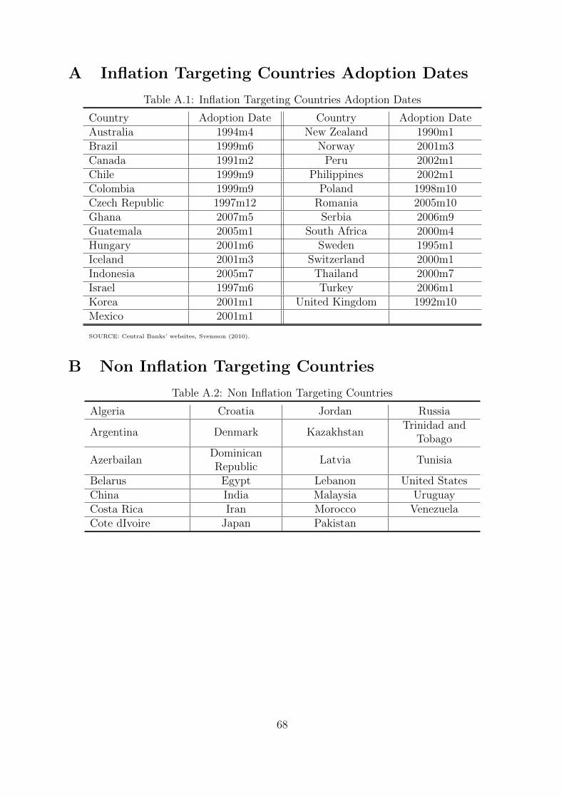
A Inflation Targeting Countries Adoption Dates

Table A.1: Inflation Targeting Countries Adoption Dates

Country Adoption Date Country Adoption Date

Australia 1994m4 New Zealand 1990m1

Brazil 1999m6 Norway 2001m3

Canada 1991m2 Peru 2002m1

Chile 1999m9 Philippines 2002m1

Colombia 1999m9 Poland 1998m10

Czech Republic 1997m12 Romania 2005m10

Ghana 2007m5 Serbia 2006m9

Guatemala 2005m1 South Africa 2000m4

Hungary 2001m6 Sweden 1995m1

Iceland 2001m3 Switzerland 2000m1

Indonesia 2005m7 Thailand 2000m7

Israel 1997m6 Turkey 2006m1

Korea 2001m1 United Kingdom 1992m10

Mexico 2001m1

SOURCE: Central Banks’ websites, Svensson (2010).

B Non Inflation Targeting Countries

Table A.2: Non Inflation Targeting Countries

Algeria Croatia Jordan Russia

Argentina Denmark KazakhstanTrinidad and

Tobago

AzerbailanDominicanRepublic

Latvia Tunisia

Belarus Egypt Lebanon United States

China India Malaysia Uruguay

Costa Rica Iran Morocco Venezuela

Cote dIvoire Japan Pakistan

68

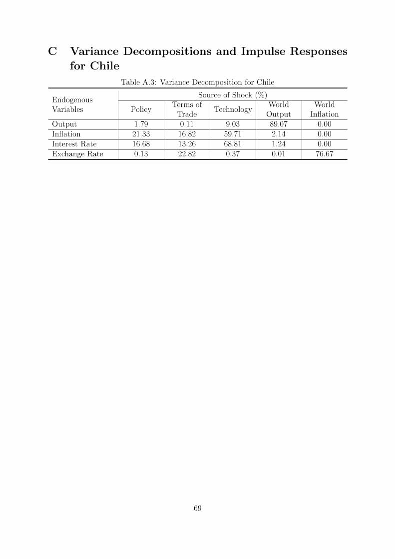
C Variance Decompositions and Impulse Responses

for Chile

Table A.3: Variance Decomposition for Chile

EndogenousSource of Shock (%)

Variables PolicyTerms of

TradeTechnology

WorldOutput

WorldInflation

Output 1.79 0.11 9.03 89.07 0.00

Inflation 21.33 16.82 59.71 2.14 0.00

Interest Rate 16.68 13.26 68.81 1.24 0.00

Exchange Rate 0.13 22.82 0.37 0.01 76.67

69

Figure A.1: Impulse Responses to a One Standard Deviation Shock for Chile

70

Essays in Open Economy Monetary Policy by Pedro Araujo...

Documents

Transcript of Essays in Open Economy Monetary Policy by Pedro Araujo...