Essays in international finance: risk, jumps and ...
195
HAL Id: tel-02524157 https://tel.archives-ouvertes.fr/tel-02524157 Submitted on 30 Mar 2020 HAL is a multi-disciplinary open access archive for the deposit and dissemination of sci- entific research documents, whether they are pub- lished or not. The documents may come from teaching and research institutions in France or abroad, or from public or private research centers. L’archive ouverte pluridisciplinaire HAL, est destinée au dépôt et à la diffusion de documents scientifiques de niveau recherche, publiés ou non, émanant des établissements d’enseignement et de recherche français ou étrangers, des laboratoires publics ou privés. Essays in international finance : risk, jumps and diversification Oussama M’Saddek To cite this version: Oussama M’Saddek. Essays in international finance : risk, jumps and diversification. Economics and Finance. Université Clermont Auvergne [2017-2020], 2018. English. NNT : 2018CLFAD009. tel-02524157
Transcript of Essays in international finance: risk, jumps and ...
HAL Id: tel-02524157https://tel.archives-ouvertes.fr/tel-02524157
Submitted on 30 Mar 2020
HAL is a multi-disciplinary open accessarchive for the deposit and dissemination of sci-entific research documents, whether they are pub-lished or not. The documents may come fromteaching and research institutions in France orabroad, or from public or private research centers.
L’archive ouverte pluridisciplinaire HAL, estdestinée au dépôt et à la diffusion de documentsscientifiques de niveau recherche, publiés ou non,émanant des établissements d’enseignement et derecherche français ou étrangers, des laboratoirespublics ou privés.
Essays in international finance : risk, jumps anddiversificationOussama M’Saddek
To cite this version:Oussama M’Saddek. Essays in international finance : risk, jumps and diversification. Economicsand Finance. Université Clermont Auvergne [2017-2020], 2018. English. NNT : 2018CLFAD009.tel-02524157

THESE DE DOCTORAT DEL’UNIVERSITE CLERMONT AUVERGNE
Ecole Universitaire de ManagementEcole Doctorale des Sciences Economiques, Juridiques, Politiques et de Gestion
Centre de Recherche Clermontois en Gestion et Management
Presentee par
Oussama M’SADDEK
Pour obtenir le titre de
DOCTEUR EN SCIENCES DE GESTION
Sujet de la these :
Essays in International Finance: Risk, Jumps and
Diversification
Soutenue le 28 septembre 2018
Composition du jury :
Directeur de these Mohamed AROURI
Professeur, Universite Cote d’Azur
Rapporteur Julien FOUQUAU
Professeur, ESCP Europe
Rapporteur Michael ROCKINGER
Professeur, HEC, Universite de Lausanne
Suffragant Fabrice HERVE
Professeur, Universite de Bourgogne
Suffragant Jerome LAHAYE
Professeur, Universite Fordham
Suffragant Benjamin WILLIAMS
Professeur, Universite Clermont Auvergne
Membre invite Sebastien LAURENT
Professeur, Universite d’Aix-Marseille


Remerciements
Je tiens ici a exprimer ma profonde gratitude a toutes les personnes qui ont rendu possible
la realisation de cette these. Je tiens tout d’abord a remercier mon directeur de these, Mon-
sieur Mohamed Arouri, pour son interet, son soutien, sa disponibilite et ses precieux conseils
durant la redaction de la these.
Je remercie egalement les membres du jury, Monsieur Julien Fouquau et Monsieur Michael
Rockinger pour avoir accepte de rapporter ma these, Monsieur Fabrice Herve, Monsieur
Jerome Lahaye et Monsieur Benjamin Williams d’en etre les suffragants. Je remercie egalement
Monsieur Sebastien Laurent pour avoir accepte de participer a l’evaluation de ce travail de
recherche.
Mes remerciements vont egalement a tous les membres de CRCGM, et en particulier les
chercheurs de la thematique ”Gouvernance et Valeur” pour leurs remarques et suggestions au
cours des seminaires mensuels du CRCGM.
Enfin, je ne pourrais finir ces remerciements sans penser a ma famille dont l’affection,
l’amour, le soutien et l’encouragement constants m’ont ete d’un grand reconfort et ont con-
tribue a l’aboutissement de ce travail.


Abstract
This thesis consists of an introductory chapter and three empirical studies that contribute
to the international finance literature by investigating the dynamics of cojumps between
major equity markets and assessing their impact on international portfolio allocation and
asset pricing.
The first study (chapter 2) examines the impact of cojumps between international stock
markets on asset holdings and portfolio diversification benefits. Using intraday index-based
data for exchange-traded funds (SPY, EFA and EEM) as proxies for international equity
markets, we document evidence of significant intraday cojumps, with the intensity increasing
during the global financial crisis of 2008-2009. The application of the Hawkes process also
shows that jumps propagate from the US and other developed markets to emerging markets.
However, the evidence of jump spillover from emerging markets to developed markets is weak.
To assess the impact of cojumps on international asset holdings, we consider a representative
American investor who allocates his wealth among one domestic risky asset, the SPY fund,
and two foreign risky assets, the EFA and EEM funds and compute the optimal portfolio com-
position from the US investor perspective by minimizing the portfolio’s risk. We find that the
demand of foreign assets is negatively correlated to jump correlation, implying that a domestic
investor will invest less in foreign markets when the frequency of cojumps between domestic
and foreign assets increases. In contrast, idiosyncratic jumps are found to increase the di-
versification benefits and foreign asset holdings in international equity portfolios. Finally, we
examine the impact of higher-order moments induced by idiosyncratic and systematic jumps
on the optimal portfolio composition by considering an investor who recognizes jump risks
as well as another investor who ignores them. Our results show that both investors have
almost the same portfolio composition, which indicates that the impact of jump higher-order
moments on optimal portfolio composition is not significant.
The second study (chapter 3) tackles the issue of pricing of both continuous and jump
risks in the cross-section of international stock returns. We contribute to the literature on

international asset pricing by considering a general pricing framework involving six separate
market risk factors. We first decompose the systematic market risk into intraday and overnight
components. The intraday market risk includes both continuous and jump parts. We then
consider the asymmetry and size effects of market jumps by separating the systematic jump
risk into positive vs. negative and small vs. large components. Using the intraday data of a
set of country exchange traded funds covering developed, emerging and frontier markets, we
show that continuous and downside discontinuous risks are positively rewarded in the cross-
section of expected stock returns during the pre-financial crisis period whereas the upside
and large jump risks are negatively priced during the crisis and post-crisis periods. We also
provide evidence on the strong negative relationship between market price movements and
market volatility changes, suggesting that both price and volatility risks share compensations
for common underlying risk factors.
The third study (chapter 4) examines how international equity markets respond to ag-
gregate market jumps at price and volatility levels. Using intraday data of ten exchange-
traded funds covering major developed and emerging markets and two international market
volatility indices (VIX and VXEEM), we show that both price and volatility jump betas are
time-varying and exhibit asymmetric effects across upside and downside market movements.
Looking at the relation between future stock market returns and aggregate market price and
volatility jumps, we measure the proportion of future excess returns explained by market price
and volatility jumps and provide evidence of a significant predictive power that market price
and volatility jumps have on future stock returns.
Overall, our results suggest that the jump risks play an important role in determining the
market risk premium and portfolio allocation decisions in an international setting.
Keywords: cojumps, international diversification, home bias, risk premium, leverage
effect, high frequency data.


Contents
1 General Introduction 2
1.1 Background . . . . . . . . . . . . . . . . . . . . . . . . . . . . . . . . . . . . . . 2
1.2 Diversification, jump and cojump risks in international stock markets . . . . . 3
1.2.1 Jump identification techniques . . . . . . . . . . . . . . . . . . . . . . . 4
1.2.2 Cojump identification techniques . . . . . . . . . . . . . . . . . . . . . . 6
1.2.3 Jumps and cojumps in equity markets . . . . . . . . . . . . . . . . . . . 6
1.2.4 International diversification in presence of correlated jumps . . . . . . . 7
1.2.5 The pricing of jump risks in the cross-section of returns . . . . . . . . . 10
1.3 Essays . . . . . . . . . . . . . . . . . . . . . . . . . . . . . . . . . . . . . . . . . 12
1.3.1 First essay . . . . . . . . . . . . . . . . . . . . . . . . . . . . . . . . . . 12
1.3.2 Second essay . . . . . . . . . . . . . . . . . . . . . . . . . . . . . . . . . 13
1.3.3 Third essay . . . . . . . . . . . . . . . . . . . . . . . . . . . . . . . . . . 14
2 Cojumps and Asset Allocation in International Equity Markets 22
2.1 Introduction . . . . . . . . . . . . . . . . . . . . . . . . . . . . . . . . . . . . . . 23
2.2 Jump and cojump identification . . . . . . . . . . . . . . . . . . . . . . . . . . . 26
2.3 Portfolio allocation problem . . . . . . . . . . . . . . . . . . . . . . . . . . . . . 29
2.3.1 Optimal portfolio composition and jump correlation . . . . . . . . . . . 30
2.3.2 Optimal portfolio composition and jump higher-order moments . . . . . 36
2.4 Data . . . . . . . . . . . . . . . . . . . . . . . . . . . . . . . . . . . . . . . . . . 41
8

CONTENTS 9
2.5 Empirical findings . . . . . . . . . . . . . . . . . . . . . . . . . . . . . . . . . . 42
2.5.1 Intraday jump identification . . . . . . . . . . . . . . . . . . . . . . . . . 42
2.5.2 Time and space clustering of intraday jumps . . . . . . . . . . . . . . . 48
2.5.3 Cojumps and optimal portfolio composition . . . . . . . . . . . . . . . . 52
2.5.4 Cojumps and the benefits of international portfolio diversification . . . 61
2.6 Conclusion . . . . . . . . . . . . . . . . . . . . . . . . . . . . . . . . . . . . . . 64
Appendix 2.A Intraday volatility pattern . . . . . . . . . . . . . . . . . . . . . . . . 71
Appendix 2.B Mean-CVaR optimization problem . . . . . . . . . . . . . . . . . . . 72
Appendix 2.C Expected power utility maximization . . . . . . . . . . . . . . . . . . 74
3 Jump Risk Premia Across Major International Equity Markets 78
3.1 Introduction . . . . . . . . . . . . . . . . . . . . . . . . . . . . . . . . . . . . . . 79
3.2 Betas estimation framework . . . . . . . . . . . . . . . . . . . . . . . . . . . . . 83
3.3 Data description . . . . . . . . . . . . . . . . . . . . . . . . . . . . . . . . . . . 86
3.4 Empirical Findings . . . . . . . . . . . . . . . . . . . . . . . . . . . . . . . . . . 89
3.4.1 Systematic cojumps . . . . . . . . . . . . . . . . . . . . . . . . . . . . . 89
3.4.2 Diffusive and jump betas . . . . . . . . . . . . . . . . . . . . . . . . . . 96
3.4.3 Risk factors and portfolio sorts . . . . . . . . . . . . . . . . . . . . . . . 98
3.4.4 Fama-MacBeth regressions . . . . . . . . . . . . . . . . . . . . . . . . . 107
3.4.5 Currency jump risk premium . . . . . . . . . . . . . . . . . . . . . . . . 111
3.4.6 Equity risk premia and the leverage effect . . . . . . . . . . . . . . . . . 115
3.5 Conclusion . . . . . . . . . . . . . . . . . . . . . . . . . . . . . . . . . . . . . . 119

Appendix 3.A Jump and cojump identification methodology . . . . . . . . . . . . . 125
4 Price and Volatility Jump Risks in International Equity Markets 130
4.1 Introduction . . . . . . . . . . . . . . . . . . . . . . . . . . . . . . . . . . . . . . 131
4.2 Betas estimation framework . . . . . . . . . . . . . . . . . . . . . . . . . . . . . 134
4.2.1 Price jump regressions . . . . . . . . . . . . . . . . . . . . . . . . . . . . 134
4.2.2 Volatility jump regressions . . . . . . . . . . . . . . . . . . . . . . . . . . 137
4.3 Data description . . . . . . . . . . . . . . . . . . . . . . . . . . . . . . . . . . . 139
4.4 Empirical Findings . . . . . . . . . . . . . . . . . . . . . . . . . . . . . . . . . . 141
4.4.1 Price and volatility cojumps . . . . . . . . . . . . . . . . . . . . . . . . . 141
4.4.2 Price jump betas . . . . . . . . . . . . . . . . . . . . . . . . . . . . . . . 145
4.4.3 Volatility jump betas . . . . . . . . . . . . . . . . . . . . . . . . . . . . . 150
4.4.4 Upside and downside jump betas . . . . . . . . . . . . . . . . . . . . . . 155
4.4.5 Predictive jump regressions . . . . . . . . . . . . . . . . . . . . . . . . . 159
4.5 Conclusion . . . . . . . . . . . . . . . . . . . . . . . . . . . . . . . . . . . . . . 167
Appendix 4.A Jump and cojump identification methodology . . . . . . . . . . . . . 171
5 General Conclusion 176
10

List of Tables
2.1 Summary statistics of jump occurrences, jump sizes and intraday returns. . . . 43
2.2 Summary statistics of jump occurrences at day level. . . . . . . . . . . . . . . . 44
2.3 Summary statistics of cojump occurrences. . . . . . . . . . . . . . . . . . . . . . 45
2.4 Summary statistics of cojump occurrences at day level. . . . . . . . . . . . . . . 45
2.5 Summary statistics of cojumps between EUR/USD exchange rate and interna-
tional equity funds. . . . . . . . . . . . . . . . . . . . . . . . . . . . . . . . . . . 46
2.6 Maximum likelihood estimation of the bivariate Hawkes model. . . . . . . . . . 51
2.7 Correlation between the daily intensity of cojumps and the optimal proportion
of the foreign assets. . . . . . . . . . . . . . . . . . . . . . . . . . . . . . . . . . 58
2.8 Correlation between the daily intensity of idiosyncratic jumps and the demand
of foreign assets. . . . . . . . . . . . . . . . . . . . . . . . . . . . . . . . . . . . 59
2.9 Multivariate jump-diffusion model estimation. . . . . . . . . . . . . . . . . . . . 60
2.10 Optimal portfolio weights using power utility maximization approach. . . . . . 61
2.11 The impact of simultaneous and idiosyncratic jumps on the optimal level of the
diversification benefit. . . . . . . . . . . . . . . . . . . . . . . . . . . . . . . . . 63
3.1 Country exchange-traded funds. . . . . . . . . . . . . . . . . . . . . . . . . . . . 87
3.2 Summary statistics of jump occurrences. . . . . . . . . . . . . . . . . . . . . . . 90
3.3 Summary statistics of systematic cojumps. . . . . . . . . . . . . . . . . . . . . . 93
3.4 Summary statistics of different betas. . . . . . . . . . . . . . . . . . . . . . . . . 97
3.5 Contemporaneous and future returns of portfolios sorted by different betas for
the period from July 2003 to December 2014. . . . . . . . . . . . . . . . . . . . 100
11

3.6 Contemporaneous and future returns of portfolios sorted by different betas
during the pre-crisis period (July 2003-June 2008). . . . . . . . . . . . . . . . . 103
3.7 Contemporaneous and future returns of portfolios sorted by different betas
during the crisis and post-crisis period (July 2008-December 2014). . . . . . . . 105
3.8 Fama-MacBeth regressions. . . . . . . . . . . . . . . . . . . . . . . . . . . . . . 110
3.9 Cojumps between stock markets and EUR/USD exchange rate. . . . . . . . . . 112
3.10 Equity and currency jump risk premia. . . . . . . . . . . . . . . . . . . . . . . . 114
3.11 Continuous and discontinuous leverage effects. . . . . . . . . . . . . . . . . . . . 119
4.1 Country exchange-traded funds and volatility indices. . . . . . . . . . . . . . . 140
4.2 Summary statistics of jump occurrences. . . . . . . . . . . . . . . . . . . . . . . 143
4.3 Summary statistics of cojump occurrences. . . . . . . . . . . . . . . . . . . . . . 144
4.4 Price jump beta estimation and tests for constancy over the full sample. . . . . 147
4.5 Price jump beta estimation over years. . . . . . . . . . . . . . . . . . . . . . . . 148
4.6 Tests of a constant price jump beta over years. . . . . . . . . . . . . . . . . . . 150
4.7 Volatility jump beta estimation and tests for constancy over the full sample. . . 151
4.8 Volatility jump beta estimation over years. . . . . . . . . . . . . . . . . . . . . 153
4.9 Tests of a constant volatility jump beta over years. . . . . . . . . . . . . . . . . 154
4.10 Positive and negative price jump betas estimation and tests for constancy over
the full sample. . . . . . . . . . . . . . . . . . . . . . . . . . . . . . . . . . . . . 156
4.11 Positive and negative volatility jump beta estimation and tests for constancy
over the full sample. . . . . . . . . . . . . . . . . . . . . . . . . . . . . . . . . . 158
12

List of Figures
2.1 Jump and cojump occurrences. . . . . . . . . . . . . . . . . . . . . . . . . . . . 47
2.2 Time and space clustering of intraday jumps. . . . . . . . . . . . . . . . . . . . 49
2.3 The variation of the optimal proportion of foreign assets. . . . . . . . . . . . . 53
2.4 Standard deviation, CVaR and correlations of domestic and foreign assets. . . . 55
2.5 The conditional diversification benefit (CDB). . . . . . . . . . . . . . . . . . . . 62
2.6 Linear regression between the conditional diversification benefit (CDB) and the
correlation of jumps. . . . . . . . . . . . . . . . . . . . . . . . . . . . . . . . . . 64
3.1 Beta distributions. . . . . . . . . . . . . . . . . . . . . . . . . . . . . . . . . . . 98
4.1 Positive and negative SPY price jumps and SPY future excess returns. . . . . . 161
4.2 Positive and negative SPY price jumps and future individual country fund
excess returns. . . . . . . . . . . . . . . . . . . . . . . . . . . . . . . . . . . . . 162
4.3 Positive and negative SPY volatility jumps and SPY future excess returns. . . 164
4.4 Positive and negative SPY volatility jumps and future individual country fund
excess returns. . . . . . . . . . . . . . . . . . . . . . . . . . . . . . . . . . . . . 165
13


Chapter 1
General Introduction
1.1 Background
This dissertation consists of an introductory chapter and three research essays that con-
tribute to the existing literature on international finance by focusing especially on the effects
of jump and cojump risks on international portfolio allocation and asset pricing. The nature
of international stock market comovements is an important issue that has been extensively
studied in the international finance literature (see, among others, Karolyi and Stulz (1996),
De Santis and Gerard (1997), Ang and Bekaert (2002)). The topic of international stock
market interdependencies has gained an increased interest among researchers for at least two
main reasons. First, the nature and degree of cross-market linkages have a direct effect on
international diversification. The modern portfolio theory suggests that diversification is an
efficient tool to minimize the portfolio’s risk. Investors, either individual or institutional, can
reduce the risk of their portfolios by holding assets that are not perfectly correlated. On the
contrary, in the context of an increased cross-market correlation, the benefit of portfolio di-
versification will be reduced. Motivated by the increased capital market integration covering
both developed and emerging markets during the last decades, many researchers questioned
if cross-country correlations would increase and thus the international diversification benefits
would decrease.
Second, the study of correlations has been also boosted by the recurrence of financial
crises that occurred in both developed and emerging countries during the last three decades.
Understanding the nature of interdependencies between international stock markets in period
of crisis is of great interest for both investors and policy makers who want to guard against
an excessive correlation between international markets, known also as contagion risk. Several
studies (Ang et al., 2006 and Lettau et al., 2014) provide evidence of a significant downside
2

1.2. Diversification, jump and cojump risks in international stock markets 3
risk in equity markets and have documented the high correlation of large down moves in
international markets (see, among others, Longin and Solnik (2001), Ang and Bekaert (2002),
Ang and Chen (2002) and Hartmann et al. (2004)).
More recently, researchers have especially focused on studying the comovement of stock
returns in the tail of the distribution, also called tail dependence or tail risk. It is well
documented in the finance literature that financial asset prices often violate the log-normality
assumptions and exhibit large discontinuities or jumps in their trajectories. Thanks to the
availability of high frequency data, the recent development of nonparametric jump detection
techniques (see, among others, Barndorff-Nielsen and Shephard (2004, 2006), Andersen et al.
(2007), Lee and Mykland (2008) and Ait-Sahalia and Jacod (2009)) provides strong evidence
in favor of the presence of jumps in asset prices. The main objective of this dissertation is to
contribute to the existing literature on international stock market correlations by empirically
investigating the dynamics of cojumps in international equity markets and assessing their
impact on portfolio allocation decisions and asset pricing.
The remainder of this introductory chapter is organized as follows. Section 1.2 goes
through the existing literature on international diversification, jump and cojump risks in
international stock markets. Section 1.3 summarizes the three essays and highlights their
main contributions.
1.2 Diversification, jump and cojump risks in international
stock markets
This section goes through the main works in the literature that motivated our study.
The objective is not to provide an exhaustive list of all studies on jump and cojump risks in
international stock markets, but to shed light on the main strands of the literature that are
directly linked to the topics addressed in this thesis.
The literature on jump and cojump risks in financial markets can be decomposed on three

1.2. Diversification, jump and cojump risks in international stock markets 4
strands. The first one focused on the issue of jump identification. The works in this era have
been motivated by the availability of high frequency data and the development of new jump
identification techniques. Others studies were interested in studying simultaneous jumps or
cojumps and developed new statistical techniques to detect the occurrence of cojumps across
assets. The tools proposed in these studies are very useful for detecting both individual and
common arrivals of jumps which is a key building block in studying jump dependencies.
The second branch of the literature examines the question of international diversification
in presence of jumps and cojumps between assets. As mentioned earlier, the main question
here is to analyze how asset allocation decisions of investors will move when considering asset
jumps’ dependencies.
The third branch of the literature explores the relationship between jumps in asset prices
with those of aggregate risk factors and develops new econometrical tools for measuring the
sensitivity of individual assets to market jumps, known also as the jump beta. These tools are
very useful in practice especially for researchers who are interested in the pricing of individual
assets and the understanding of the cross-section of asset returns.
1.2.1 Jump identification techniques
Numerous detection techniques have been proposed in the literature to resolve price jump
identification issues. These techniques are often derived from the statistical test theory. They
aim to study the dynamics of jumps’ arrivals using high frequency data. The seminal work
in this area was Barndorff-Nielsen and Shephard (2004, 2006) who distinguish between two
measures of integrated variance. The first one takes into account the jump component of the
price process when measuring the integrated variance while the second one is a jump robust
measure. Authors develop a nonparametric test which indicates if a sample contains jumps
using the reported measures.
Lee and Mykland (2008) notice the impact of the sensitivity of intraday volatility patterns
on Barndorff-Nielsen and Shephard nonparametric test, that leads to spurious detection of

1.2. Diversification, jump and cojump risks in international stock markets 5
jumps. The basic idea behind their statistical test is to distinguish movements of the realized
return that are caused by jumps from those that are induced by a high level of volatility. Thus,
they develop a new statistical test by scaling returns by a local volatility measure. Bajgrowicz
et al. (2015) also propose a technique to eliminate spurious detection of jumps on available
test statistics using specific thresholds. Mancini (2001, 2009) has also developed a nonpara-
metric test for measuring jump arrival times from high-frequency data using threshold-based
methods.
A different approach (known as the ”swap variance” approach) was proposed by Jiang and
Oomen (2008) who consider the third and higher-order return moments to identify jumps at
day level. They were inspired from the ”swap variance” replication strategy to construct their
statistical test. Ait-Sahalia and Jacod (2009) also examine the difference between high order
moments of returns at two different sampling frequencies to detect jumps in a daily basis.
Although these statistical tests are designed to detect the same jumps, studies show that
their results are often incoherent. Schwert (2008) finds, for example, that the amount and
the timing of jumps depend on the choice of the sampling frequency. In an attempt to find
the optimal level of sampling frequency, he mentions that the microstructure noise has a
significant impact on different test statistics.1 He proposes to sample market data at intervals
of five to eleven minutes to reduce the effects of microstructure noise. Dumitru and Urga
(2012) provide a comparison study between various univariate tests through Monte Carlo
procedures and find that the intraday jump test of Lee and Mykland outperforms other jump
identification procedures especially when the volatility is not high. The test of Lee and
Mykland has also the advantage to identify jumps intradaily compared to others jump tests
that have been designed to determine if a day (or a given time window) contains price jumps.
1The microstructure noise is the deviation of the asset price from its fundamental value due to marketfrictions such as bid-ask bounce, latency, and asymmetric information.

1.2. Diversification, jump and cojump risks in international stock markets 6
1.2.2 Cojump identification techniques
In addition to univariate jump identification techniques, econometric tools have been devel-
oped to detect common arrivals of asset jumps, also called multivariate jump tests. However,
the literature on cojump identification is relatively recent and scarcer compared to univariate
jump tests. The most intuitive way to detect cojumps is to identify jump occurrences for
each individual asset using an univariate jump test and then apply the co-exceedance rule
proposed by Bae et al. (2003). A cojump is identified if two or more assets jump within the
same intraday time interval. Bollerslev et al. (2008) use the mean of cross products of returns
of a large number of stocks as a test statistic to detect common arrival of jumps at portfolio
level. Their test statistic is sensitive to the number of stocks considered in the portfolio.
Indeed, a large number of stocks is required to diversify away asset idiosyncratic jumps.
Jacod and Todorov (2009) develop a bivariate jump indentification test using the ratio
of power variation estimators. However, their approach can only be applied to detect if a
particular day contains cojumps. Gobbi and Mancini (2012) propose a daily cojump test by
applying thresholding techniques. Gnabo et al. (2014) use the product of assets’ intraday re-
turns and parametric bootstrapping techniques to identify intraday cojumps. Their approach
complements the univariate jump detection tests in the sense that it aims to identify poten-
tial cojumps, which are not, detected through univariate jump tests. However, Gnabo et al.
(2014) show that univariate tests remain satisfactory and best-suited for detecting jumps and
cojumps as long as the jumps sizes are sufficiently large and have the same sign as the assets’
correlation.
1.2.3 Jumps and cojumps in equity markets
Motivated by the development of nonparametric jump detection tests, researchers exam-
ine the dynamics of jumps in different stock markets. Gilder et al. (2012) use univariate
jump detection techniques to identify intraday jumps in the US stock market and examine
the frequency of cojumps between individual stocks and the market portfolio. They find a

1.2. Diversification, jump and cojump risks in international stock markets 7
tendency for a relatively large number of stocks to be involved in systematic cojumps, which
are defined as cojumps between a stock and market portfolio. Lahaye et al. (2010) and Evans
(2011) examine the link between asset cojumps and new macro announcements and find that
cojumps are partially associated with macroeconomic news. Bormetti et al. (2015) study
the dynamics of intraday jumps in the Italian stock market and show that Hawkes one-factor
model is more suitable to capture the high synchronization of jumps across assets than the
multivariate Hawkes model (1971). Using daily data, Ait-Sahalia et al. (2015) develop a
multivariate Hawkes jump-diffusion model to capture the propagation of jumps over time
and across markets. They provide strong evidence for jumps to arrive in clusters within the
same market and to propagate to other international stock markets. Pukthuanthong and Roll
(2015) also use daily data to examine jump correlation across international stock markets.
In the first essay, we extend the existing literature by studying the dynamics of jumps in
an international setting. Our approach is based on the use of high frequency data and the
application of nonparametric jump identification tests. We also examine the time (within
same market) and space (across markets) clustering properties of intraday jumps using the
multivariate Hawkes model.
1.2.4 International diversification in presence of correlated jumps
International stock markets are characterized by jumps that have tendency to occur at the
same time across markets especially in bearish market conditions marked by large downturns
and high volatility. This excessive correlation between jumps leads researchers to question
whether the jump risk reduces the gains from the international diversification. Das and Uppal
(2004) examine this question by considering a multivariate system of jump-diffusion processes
where jumps are infrequent and occur simultaneously across assets. They find that systemic
jump risk reduces the gains of portfolio diversification especially if the considered portfolio
includes a risk free asset. Cvitani et al. (2004) consider the optimal portfolio strategy of a
representative investor with CRRA utility where the risky asset is modeled as a pure jump
process with non-trivial higher moments. They find that ignoring higher moments in the

1.2. Diversification, jump and cojump risks in international stock markets 8
portfolio optimization problem leads to an over-investment in risky assets and results in a
substantial wealth loss. Ait Sahalia et al. (2009) examine the problem of portfolio allocation
in presence of jumps and propose a closed-form solution for it.
The benefits from international portfolio diversification have been widely documented in
the finance literature (see, among others, Grubel (1968), Levy and Sarnat (1970), Lessard
(1973), and Solnik (1974)). However, studies show that in practice investors have tendency
to overweight their portfolios with assets from their home country market, meaning that
those portfolios tend to be less diversified internationally than would be optimal according to
modern portfolio theory (Markowitz, 1952). In the finance literature, this lack of international
portfolio diversification is called the home bias puzzle.
The equity home bias was first documented by French and Poterba (1991). They studied
the home bias phenomenon in five major countries and they found that at the end of 1989,
US investors hold more than 92% of their equity in domestic stock (Japan, 95%; United
Kingdom, 92%; Germany, 79% and France, 89%). Tesar and Werner (1998) show the same
figures. These empirical data are largely different from those predicted by theoretical studies
that demonstrate that the share of domestic assets in optimal portfolio composition should
be in line with the share of the domestic equity market compared to the total world equity
market. More recently, many researchers studied the evolution of the phenomenon over the
past three decades. Karolyi and Stulz (2003) found that international diversification has
increased slightly for US investors from 1973 through 2001. This decrease in home bias could
be explained by changes that experienced equities market in the nineties including the advent
of internet, the development of emerging markets, deregulation and markets liberalization.
In spite of this decrease in home bias, several studies report that investors are still far from
taking all the gains from international diversification and differences between the theoretical
share of foreign assets that should be held by investors and the real share effectively held are
largely disproportionate.
The home bias puzzle was extensively studied in the financial literature and there have

1.2. Diversification, jump and cojump risks in international stock markets 9
been various theoretical explanations that were given to rationalize investors’ behaviour and
thus the lack of international diversification observed in financial markets.2 A first potential
explanation for equity home bias is that domestic equities provide a better hedge for risks
that are home-country specific such as domestic inflation risk, exchange rate risk and hedges
against wealth that is not traded in capital markets. Empirical studies show that there is a
weak correlation between domestic stock returns and domestic inflation rate (exchange rate,
non-tradable income) indicating that hedging domestic risks fails to explain the observed
home bias.
An alternative explanation for international under-diversification is the existence of various
barriers and relatively important transaction costs for foreign investments. However, none
of the studies that consider barriers and transaction costs as an explanation to home bias
succeeds to provide plausible empirical proofs. Moreover, recent studies show that costs and
barriers to foreign investments have decreased considerably due to market liberalization in the
early nineties. Thus, the home bias in equities cannot be explained by international capital
controls or transaction costs.
A different explanation is suggested by recent empirical studies (Chan et al., 2005) that
consider information asymmetries between domestic and foreign investors as the main cause of
home bias. In order to examine the link between information asymmetries and international
portfolio choice, researchers mainly use econometric regression models to measure the impact
of each explanatory variable. The physical distance between two countries or the fact to share
a common language or culture is often used as a proxy for information asymmetries in those
models. Contrary to the information-based explanation of home bias, others researchers
criticize the fact that this theory implicitly assumes that domestic investors have superior
access to the domestic market in an environment of global information access. It seems that
there is no consensus between researchers on the role of information asymmetries as a cause
to the observed home bias. This is also related to difficulties to provide a convincing empirical
study about the effect of information asymmetries on the portfolio choice due to the lack in
2Refer to Lewis (1999) for a review of the home bias literature.

1.2. Diversification, jump and cojump risks in international stock markets 10
practice of data necessary to measure these asymmetries.
The explanations reported below are based on the assumption of perfectly rational be-
haviour of individuals. As it seems that the home bias cannot only be explained by rational
behaviour of investors, recent studies rely on recent findings of behavioral finance in order to
explain international under-diversification. Researchers examined if the irrational behaviour
of investors could be explained by behavioural biases such as overconfidence, familiarity with
domestic stocks, patriotism and specific investor characteristics (sophisticated investor or not,
age, gender, income).
The puzzle has led to an extensive research effort in both traditional and behavioral fi-
nance. So far, several explanations have been presented, but a solution generally accepted
by the researchers remains elusive. In the first essay, we contribute to the existing literature
on the lack of international diversification by investigating how the cojumps between interna-
tional stock markets will affect the demand of foreign assets and the gains from international
diversification. To the best of our knowledge, we are the first study that examines the impact
of intraday cojumps on portfolio allocation decisions in an international setting. Our approach
is based on the identification of cojumps using high frequency data. We use mean-variance
and mean-CVaR approaches to determine the optimal portfolio composition and examine
how the demand of foreign assets varies with jumps’ correlation. The impact of higher-order
moments induced by jumps on the optimal portfolio composition is also examined.
1.2.5 The pricing of jump risks in the cross-section of returns
The finance theory establishes that investors should be compensated for bearing non-
diversifiable risks. Aggregate market jumps are a potential source of systematic risk. There-
fore, understanding how individual assets are linked to aggregate market jumps plays a key
role in measuring, managing and pricing jump risks. In this field, Bollerslev et al. (2016)
and Li et al. (2017) develop new econometrical tools for estimating the sensitivity of indi-
vidual assets to market jumps. Using these new tools, Bollerslev et al. (2016) and Alexeev

1.2. Diversification, jump and cojump risks in international stock markets 11
et al. (2017) document that the jump risk carries a significant positive premium. However,
the scope of their empirical works is restricted to the US market. Using option data and by
constructing suitable option trading strategies, Cremers et al. (2015) provide evidence that
both aggregate jump and volatility are priced risk factors, but both of them carry negative
market risk prices.
More recently, studies (Bandi and Reno (2016), Jacod and Todorov (2010), Todorov and
Tauchen (2011)), show that jumps in prices are often associated with strongly anti-correlated,
contemporaneous, discontinuous changes in volatility, suggesting that both the price and
volatility jump risks are derived by common underlying risk factors and thus should be handled
jointly by investors. Other studies (Bandi and Reno (2016), Davies (2016)) suggest that
market volatility jumps are also a source of systematic risk and they should be priced in the
cross-section of stock returns.
The asset pricing literature that investigates the role of tail risks on explaining the cross-
section of stock returns worldwide also includes Weigert (2016) who provides evidence of a
significant positive premium for holding stocks with a strong sensitivity to extreme market
downturns, with a risk premium particularly high in countries with higher income per capita
and negative market skewness. In contrast, Oordt and Zhou (2016) find the reward for holding
stocks that strongly comove with the market during extreme market crashes is not significant.
Their study is, however, limited to the US stock market.
In the second essay, we contribute to the existing literature by decomposing the non-
diversifiable market risk into continuous and discontinuous components and systematic jump
risks into positive vs. negative and small vs. large components. We examine their associ-
ation with equity risk premia across major equity markets. To the best of our knowledge,
we are the first study that examines the market risk across major developed, emerging and
frontier markets using a general pricing framework involving six separate market betas measur-
ing the sensitivity of individual country stock markets to respectively continuous, overnight,
discontinuous up, discontinuous down, discontinuous small and discontinuous large intraday

1.3. Essays 12
movements of the market. As jumps in prices are closely linked to jumps in the volatility, we
study, in the third essay, how developed and emerging markets react to jumps of an aggregate
market index both at price and volatility levels and examine the role of market price and
volatility jumps in forecasting international stock market returns.
1.3 Essays
1.3.1 First essay
The first essay aims to examine the impact of cojumps between international stock markets
on asset holdings and portfolio diversification benefits. The paper extends previous studies
that investigate how international diversification varies with the correlation between stock
markets by focusing specifically on the role of cojumps. It also contributes to the existing
literature by studying the dynamics of intraday jumps in an international setting.
Our empirical investigation is based on the use of intraday returns for three interna-
tional exchange-traded funds, SPY, EFA, and EEM, which respectively aim to replicate the
performance of three international equity market indices: S&P 500, MSCI EAFE (Europe,
Australasia and Far East), and MSCI Emerging Markets. The data covers the period going
from January 2008 to October 2013. We apply the univariate jump identification test of
Lee and Mykland (2008) to identify the intraday jumps of the three funds. In order to cap-
ture the dependency between the occurrences of the detected jumps, we employ the bivariate
Hawkes process (1971) which is appropriate to model the time and space clustering features of
jumps. Under this analysis, we find jumps from the US propagate to other developed markets
and emerging markets. However, the evidence of jump spillover from emerging markets to
developed markets is weak.
To assess the impact of cojumps on international asset holding, we consider a represen-
tative American investor who allocates his wealth among one domestic risky asset, the SPY
fund, and two foreign risky assets, the EFA and EEM funds. We then compute the optimal
portfolio composition from the US investor perspective by minimizing the portfolio’s risk.

1.3. Essays 13
Once the optimal composition is determined, we examine how the demand of foreign assets
varies with the jump correlation or cojumps. We find that the demand of foreign assets is
negatively correlated to jump correlation, implying that a domestic investor will invest less in
foreign markets when the frequency of cojumps between domestic and foreign assets increases.
We also uncover the negative link between the intensity of cojumps and the conditional di-
versification benefit measure suggested by Christoffersen et al. (2012). Putting differently,
the excessive jump correlation increases the cross-market comovements, and therefore reduces
the international diversification benefit and leads investors to prefer home assets. In contrast,
we find that idiosyncratic jumps have a positive effect on foreign asset holding and diver-
sification benefits, implying that country-specific jumps are a potential source of portfolio
diversification for investors. Finally, we examine the impact of higher-order moments (skew-
ness, co-skewness, kurtosis, and co-kurtosis) induced by idiosyncratic and systematic jumps
on the optimal portfolio composition by considering an investor who recognizes idiosyncratic
and systematic jump risks and assumes that asset returns are given by a multivariate jump-
diffusion process as well as another investor who ignores jumps and assumes a pure-diffusion
process for asset returns. Our results show that both investors have almost the same portfo-
lio composition, which indicates that the impact of jump higher-order moments on optimal
portfolio composition is not significant.
1.3.2 Second essay
The second research paper tackles the issue of pricing of both continuous and jump risks
in the cross-section of international stock returns. We contribute to the literature on interna-
tional asset pricing by considering a general pricing framework involving six separate market
risk factors. We first decompose the systematic market risk into intraday and overnight
components. The intraday market risk includes both continuous and jump parts. We then
consider the asymmetry and size effects of market jumps by separating the systematic jump
risk into positive vs. negative and small vs. large components.
The empirical investigation relies on the intraday data of a set of 37 country exchange-

1.3. Essays 14
traded funds covering developed, emerging and frontier markets from July 2003 to December
2014. We follow Todorov and Bollerslev (2010)’s methodology to estimate the exposure of each
country fund returns towards the systematic market diffusive and jump risks. We examine
the cross-sectional relation between estimated betas and return by forming portfolios ranked
on the basis of market betas. We find that there is a positive link between the returns of the
sorted portfolios and different factors of risk (except the overnight beta) during the pre-crisis
period going from July 2003 to June 2008. During the crisis and pre-crisis period (July 2008
to December 2014), we observe an inversion of the patterns of realized returns for portfolios
sorted on jump betas (expect for discontinuous downside beta), with a negative relation being
more pronounced for discontinuous positive and large betas. This result is consistent with an
increasing investor appetite for equities that positively comove with large and positive market
jumps during periods of market turmoil. These equities will help investors to better hedge
against large movements of market and thus would require lower expected returns.
In order to assess the price of bearing continuous and jump market risks, we follow Fama
and MacBeth (1973)’s approach by running a set of cross-sectional regressions in a monthly
basis. The results of the cross-sectional Fama and MacBeth (1973) regressions are in line with
the portfolio sorting findings. We mainly find that continuous and downside discontinuous
risks are positively rewarded in the cross-section of expected stock returns during the pre-
crisis period whereas the upside and large jump risks are negatively priced during the crisis
and post-crisis periods. By studying the return-volatility relationship over the sample period,
we provide evidence on the strong negative covariation between market price movements
(both continuous and downside discontinuous) and market volatility changes during the pre-
crisis period, suggesting that both price and volatility risks share compensations for common
underlying risk factors during the pre-crisis period.
1.3.3 Third essay
The third research article complements the first two essays by examining how interna-
tional equity markets respond to aggregate market jumps at both price and volatility levels.

1.3. Essays 15
Motivated by the recent development of jump regression techniques (Li et al. (2017) and
Davies (2016)), we examine the linear relationship between individual stock markets and an
aggregate market proxy at jump times at both price and volatility levels.
The empirical work is based on two sets of high frequency data. The first set is composed
of ten exchange-traded funds covering major developed and emerging markets. The second
set is composed of two volatility indices: the Chicago Board of Options Exchange’s (CBOE)
Volatility Index (VIX) and CBOE Emerging Markets ETF Volatility Index (VXEEM) serving
as proxies for respectively the developed and emerging market volatilities. The sample covers
the period going from January 2008 to May 2015. By applying the techniques proposed by
Andersen et al. (2007) and Lee and Mykland (2008), we identify intraday jumps and cojumps
of all funds and volatility indices in the sample and find that simultaneous jumps between
individual country funds and two volatility indices have opposite signs, with a higher propor-
tion of positive volatility and negative return cojumps, suggesting a strong anti-correlation
between market volatility jumps and the asset returns when the market is downward and its
volatility is high.
By considering jump regression techniques proposed by Li et al. (2017) and Davies (2016),
we estimate the sensitivity of individual country markets to respectively market price and
volatility jumps and show that both price and volatility jump betas are time-varying over the
period of study. We also document asymmetric effects across upside and downside market
movements for the price jump betas. The results found for the upside and downside volatility
jump betas, are, however, inconclusive.
Looking at the relation between future stock market returns and aggregate market price
and volatility jumps, we measure the proportion of future excess returns explained by market
price and volatility jumps and provide evidence of a significant predictive power that market
price and volatility jumps have on future stock returns, with a stronger degree of predictability
obtained with market price jumps.
References
Ait-Sahalia, Y., Cacho-Diaz, J., and Laeven, R., 2015. Modeling financial contagion using
mutually exciting jump processes. Journal of Financial Economics 117, 585-606.
Ait-Sahalia, Y., Cacho-Diaz, J., and Hurd, T. R., 2009. Portfolio Choice with Jumps: A
Closed-Form Solution. The Annals of Applied Probability 19, 556-584.
Ait-Sahalia, Y. and Jacod, J., 2009. Testing for jumps in a discretely observed process. The
Annals of Statistics 37, 184-222.
Alexeev,V., Dungey, M. and Yao, W., 2017. Time-varying continuous and jump betas: The
role of firm characteristics and periods of stress. Journal of Empirical Finance 20, 1-20.
Andersen, T.G, Bollerslev, T., and Dobrev, D., 2007. No-arbitrage semi-martingale restric-
tions for continuous-time volatility models subject to leverage effects, jumps and i.i.d. noise:
Theory and testable distributional implications. Journal of Econometrics 138 (1), 125-180.
Ang, A., and Bekaert, G., 2002. International Asset Allocation with Regime Shifts. Review
of Financial Studies 15, 1137-1187.
Ang, A. and Chen, J., 2002. Asymmetric correlations of equity portfolios. Journal of Financial
Economics 63, 443-494.
Ang, A., Chen, J., and Xing, Y., 2006. Downside Risk. Review of Financial Studies 19 (4),
1191-1239.
Bae, K.-H., Karolyi, G. A. and Stulz, R. M., 2003. A new approach to measuring financial
contagion. Review of Financial Studies 16, 717-763.
Bajgrowicz, P., Scaillet, O., and Treccani, A., 2015. Jumps in High-Frequency Data: Spurious
Detections, Dynamics, and News. Management Science, 2198-2217.
Bandi, F.M., and Reno, R. 2016. Price and volatility co-jumps. Journal of Financial Economics
119, 107-146.
16

REFERENCES 17
Barndorff-Nielsen O. E. and Shephard, N., 2004. Power and bipower variation with stochastic
volatility and jumps. Journal of Financial Econometrics 2, 1-37.
Barndorff-Nielsen, O. E. and Shephard, N., 2006. Econometrics of testing for jumps in financial
economics using bipower variation. Journal of Financial Econometrics 4, 1-30.
Bollerslev, T., Law, T. H., Tauchen, G., 2008. Risk, jumps, and diversification. Journal of
Econometrics 144(1), 234-256.
Bollerslev T., Todorov V., and Li S. Z., 2016, Roughing up Beta: continuous vs. discontinuous
betas, and the cross-section of expected stock returns. Journal of Financial Economics 120
(3), 464-490.
Bormetti, G., Calcagnile, L.M., Treccani, M., Corsi, F., Marmi, S., Lillo, F., 2015. Modelling
systemic price cojumps with hawkes factor models. Quantitative Finance 15, 1137-1156.
Chan, K. , Covrig, V., and Ng, L., 2005. What Determines the Domestic Bias and Foreign
Bias? Evidence from Mutual Fund Equity Allocations Worldwide. Journal of Finance 60,
1495-1534.
Christoffersen, P., Errunza, V., Langlois, H., and Jacobs, K., 2012. Is the Potential for Inter-
national Diversification Disappearing? Review of Financial Studies 25, 3711-3751.
Cremers, M., Halling, M. and Weinbaum, D., 2015. Aggregate Jump and Volatility Risk in
the Cross-Section of Stock Returns. The Journal of Finance 70 (2), 577-614.
Cvitanic, J., Polimenis, V. and Zapatero, F., 2008. Optimal portfolio allocation with higher
moments. Annals of Finance 4, 1-28.
Das, S., Uppal, R., 2004. Systemic Risk and International portfolio choice. Journal of Finance
59, 2809-2834.
Davies, R., 2016. Volatility Jump Regressions. Working paper, Duke university.
De Santis, G. and Gerard, B., 1997. International asset pricing and portfolio diversification
with time-varying risk, Journal of Finance 52 (5), 1881-1912.

REFERENCES 18
Dumitru, A.M. and Urga, G., 2012. Identifying jumps in financial assets: A comparison
between nonparametric jump tests. Journal of Business and Economic Statistics 30 (2),
242-255.
Evans, K.P. , 2011. Intraday jumps and US macroeconomic news announcements. Journal of
Banking and Finance 35 (10).
Fama, E. F. and MacBeth, J. D, 1973. Risk, Return, and Equilibrium: Empirical Tests.
Journal of Political Economy 81 (3), 607-636.
French, K., and Poterba, J., 1991. Investor Diversification and International Equity Markets.
American Economic Review 8, 222-226.
Gilder, D., Shackleton, M., and Taylor, S., 2012. Cojumps in Stock Prices: Empirical Evi-
dence. Journal of Banking and Finance 40, 443-459.
Gnabo, J., Hvozdyk, L., and Lahaye, J., 2014. System-wide tail comovements: A bootstrap
test for cojump identification on the S&P500, US bonds and currencies. Journal of Inter-
national Money and Finance 48, 147-174.
Gobbi, F., and Mancini, C., 2012. Identifying the Brownian Covariation From the Co-jumps
given discrete observations. Econometric theory, 28, 249273.
Grubel, H., 1968. Internationally diversified portfolios: Welfare gains and capital flows. Amer-
ican Economic Review 58, 1299-1314.
Hartmann, P., Straetmans, S. and de Vries, C., 2004. Asset market linkages in crisis periods.
Review of Economics and Statistics 86, 313-326.
Hawkes, A.G., 1971. Spectra of some self-Exciting and mutually exciting point Processes.
Biometrika 58, 83-90.
Jacod, J., Todorov, V., 2010. Do price and volatility jump together? The Annals of Applied
Probability 20, 1425-69.

REFERENCES 19
Jacod, J., and Todorov, V., 2009. Testing for Common Arrivals of Jumps for Discretely
Observed Multidimensional Processes. The Annals of Statistics 37, 1792-1838.
Jiang G. J. and Oomen, R. C. A., 2008. Testing for jumps when asset prices are observed
with noise - A swap variance approach. Journal of Econometrics 144, 352-370.
Karolyi, A., and Stulz, R., 1996. Why do markets move together? An investigation of U.S.-
Japan stock return comovements, Journal of Finance 51 (3), 951-986.
Karolyi, A. and Stulz, R., 2003. Are Financial Assets Priced Locally or Globally? Handbook
of the Economics of Finance 1, 975-1020.
Lahaye J., Laurent, S., and Neely, C.J., 2010. Jumps, cojumps and macro announcements.
Journal of Applied Econometrics 26, 893-921.
Lee S. S. and Mykland, P.A., 2008. Jumps in financial markets: A new nonparametric test
and jump dynamics. Review of Financial Studies 21, 2535-2563.
Lessard, D., 1973. World, national and industry factors in equity returns. Journal of Finance
29, 379-391.
Lettau, M., Maggiori, M. and Weber, M., 2014: Conditional Risk Premia in Currency Markets
and Other Asset Classes. Journal of Financial Economics 114 (2), 197-225.
Levy, H. and Sarnat, M., 1970. International diversification of investment portfolios. American
Economic Review 60, 668-675.
Lewis, Karen K., 1999, Trying to Explain Home Bias in Equities and Consumption, Journal
of Economic Literature 37, 571-608.
Li, J., Todorov, V., Tauchen, G., 2017. Jump Regressions. Econometrica 85, 173-195.
Longin, F., and Solnik B., 2001, Extreme Correlation of International Equity Markets, Journal
Finance 56, 649-676.

REFERENCES 20
Mancini, C., 2001. Disentangling the Jumps of the Diffusion in a Geometric Jumping Brownian
Motion. Giornale dell’Istituto Italiano degli Attuari, LXIV, 19-47.
Mancini, C., 2009. Non-Parametric Threshold Estimation for Models With Stochastic Diffu-
sion Coefficient and Jumps, Scandinavian Journal of Statistics 36, 270-296.
Markowitz, H., 1952. Portfolio selection. The journal of finance 7, 77-91.
Oordt, M and Zhou, C., 2016. Systematic tail risk. Journal of Financial and Quantitative
Analysis 51, 685-705.
Pukthuanthong, K., and Roll, R., 2015. Internationally correlated jumps. Review of Asset
Pricing Studies 5, 92-111.
Schwert, M., 2008. Problems in the Application of Jump Detection Tests to Stock Price Data.
Duke University Senior Honors Thesis.
Solnik, B., 1974. Why not diversify internationally rather than domestically. Financial Ana-
lysts Journal, 48-53.
Tesar, L.L., and Werner, I.M., 1998. The Internationalization of Securities Markets Since the
1987 Crash. Brookings-Wharton Papers in Financial Services, 283-349.
Todorov, V. and Bollerslev, T., 2010. Jumps and Betas: A New Framework for Disentangling
and Estimating Systematic Risks. Journal of Econometrics 157, 220-235.
Todorov, V., Tauchen, G., 2011. Volatility jumps. Journal of Business and Economic Statistics
29, 356-371.
Weigert, F., 2016. Crash Aversion and the Cross-Section of Expected Stock Returns World-
wide. The Review of Asset Pricing Studies 6, 135-178.


Chapter 2
Cojumps and Asset Allocation in International Eq-
uity Markets1
Abstract
This paper examines the patterns of intraday cojumps between international equity markets
as well as their impact on international asset holdings and portfolio diversification benefits.
Using intraday index-based data for exchange-traded funds as proxies for international equity
markets, we document evidence of significant cojumps, with the intensity increasing during
the global financial crisis of 2008-2009. The application of the Hawkes process also shows that
jumps propagate from the US and other developed markets to emerging markets. Correlated
jumps are found to reduce diversification benefits and foreign asset holdings in minimum risk
portfolios, whereas idiosyncratic jumps increase the diversification benefits of international
equity portfolios. In contrast, the impact of higher-order moments induced by idiosyncratic
and systematic jumps on the optimal composition of international portfolios is not significant.
Keywords: Cojumps; Foreign asset holdings; International diversification.
1A paper based on this chapter has been accepted for publication in Journal of Economic Dynamics andControl.
22

2.1. Introduction 23
2.1 Introduction
It is now well established in the finance literature that price discontinuities or jumps
should be taken into account when studying asset price dynamics and allocating funds across
assets (Bekaert et al., 1998; Das and Uppal, 2004; Guidolin and Ossola, 2009; Branger et
al., 2017). In this regard, the recent development of non-parametric jump identification tests
has enabled jump detection in financial asset prices. The seminal works in this area include
Barndorff-Nielsen and Shephard (2004; 2006a) who test for the presence of jumps at the daily
level using measures of bipower variation. The same family of intraday jump identification
procedures includes the tests developed by, among others, Jiang and Oomen (2008), Andersen
et al. (2012), Corsi et al. (2010), Podolskij and Ziggel (2010), and Christensen et al. (2014).
Andersen et al. (2007) and Lee and Mykland (2008) have developed techniques to identify
intraday jumps using high frequency data. All of these jump detection techniques provide
empirical evidence in favor of the presence of asset price discontinuities or jumps.
More recently, researchers have been interested in studying cojumps between assets (Dungey
et al., 2009; Lahaye et al., 2010; Dungey and Hvozdyk, 2012; Pukthuanthong and Roll, 2015;
Ait-Sahalia and Xiu, 2016). For instance, Gilder et al. (2012) examine the frequency of
cojumps between individual stocks and the market portfolio. They find a tendency for a
relatively large number of stocks to be involved in systematic cojumps, which are defined as
cojumps between a stock and market portfolio. Lahaye et al. (2010) show that asset cojumps
are partially associated with macroeconomic news announcements. Ait-Sahalia et al. (2015)
develop a multivariate Hawkes jump-diffusion model to capture jumps propagation over time
and across markets. They provide strong evidence for jumps to arrive in clusters within the
same market and to propagate to other international markets. Bormetti et al. (2015) find
that Hawkes one-factor model is more suitable to capture the high synchronization of jumps
across assets than the multivariate Hawkes model.
Our study furthers the above-mentioned literature in two ways. First, we empirically
investigate intraday cojumps between international equity markets. Second, we show their

2.1. Introduction 24
impact on international asset allocation and portfolio diversification benefits. To the best
of our knowledge, we are the first study that examines the impact of intraday cojumps on
portfolio allocation decisions in an international setting. Past studies focus more on the im-
pact of return correlation without separating between continuous and jump parts. Modern
portfolio theory suggests that international diversification is an effective way to minimize
portfolio risks given that international assets are often less correlated and driven by different
economic factors. However, one might expect that cojumps can lead to an increase in the
correlation between these international assets and thus reduce the benefit from international
diversification. Inversely, if price jumps of different assets do not occur simultaneously, they
are categorized as idiosyncratic jumps and will not affect portfolio allocation decisions in an
international setting. Choi et al (2017) show, in contrast to traditional asset pricing theory
and in support of information advantage theory, concentrated investment strategies in inter-
national markets are associated with higher risk-adjusted returns. Our study complements
their study by showing investors prefer concentrated portfolios tilted toward home market
because cojumps between home and foreign stock markets significantly reduce diversification
benefits.
Accordingly, a risk-averse investor who holds an international portfolio is exposed to two
types of jump risks: cojump or systematic jump risk (jumps common to all markets) and
idiosyncratic jump risk (jumps specific to one market). If an investor’s portfolio is well
diversified, the idiosyncratic jump risk will be reduced or even eliminated. On the other hand,
the cojump risk cannot be eliminated through diversification, thus making its identification
central to asset pricing, asset allocation and portfolio risk hedging. Identifying cojumps is also
important to policy makers attempting to propose the policies to stabilize financial markets.
Our empirical tests rely on the use of intraday returns for three dedicated international
exchange-traded funds (ETFs) – SPY, EFA, and EEM – which respectively aim to replicate
the performance of three international equity market indices: S&P 500, MSCI EAFE (Europe,

2.1. Introduction 25
Australasia and Far East), and MSCI Emerging Markets.2 We use the technique proposed
by Andersen et al. (2007) and Lee and Mykland (2008) to empirically identify all intraday
jumps and cojumps of the three funds from January 2008 to October 2013. Lee and Mykland
(2008) show that the power of their non-parametric jump identification test increases with the
sampling frequency and that spurious detection of jumps is negligible when high frequency
data are used. Unlike Ait-Sahalia et al. (2015) who use low frequency data to study the
dynamics of jumps, we employ a bivariate Hawkes model to reproduce the time clustering
features of intraday jumps and the dynamics of their propagation across markets. The appli-
cation of the Hawkes process allows us to capture the dependence between the occurrences of
jumps which cannot be reproduced by, for example, the standard Poisson process, owing to
the hypothesis of independence of the increments (i.e., the numbers of jumps on disjoint time
intervals should be independent). Under this analysis, we find jumps from the US propagate
to other developed markets and emerging markets. However, the evidence of jump spillover
from emerging markets to developed markets is weak.
Finally, we assess the impact of cojumps on international portfolio allocation by con-
sidering a domestic risk-averse investor who selects the portfolio composition based on one
domestic asset and two foreign assets in a way to maximize his expected utility.3As investors
are concerned about negative movements of asset returns, we take the risk of extreme events
into account using the Conditional Value-at-Risk or CVaR (Rockafellar and Uryasev, 2000)
as a risk measure in our portfolio allocation problem. Unlike the standard mean-variance
approach, which typically underestimates the risk of large movements of asset returns, the
mean-CVaR approach allows us to provide a fairly accurate estimate of the downside risk
induced by negative cojumps of asset returns. As to cojumps, we apply two approaches to
assess how assets jumps are linked to each other. The first one is cojump intensity measure
obtained from the co-exceedance rule (Bae et al., 2003) and univariate jump identification
tests proposed by Andersen et al. (2007) and Lee and Mykland (2008). The second one
2S&P 500 index is used as a proxy for the US market. MSCI EAFE index is the benchmark for developedmarkets excluding the US and Canada, whereas the MSCI Emerging Markets is used to capture the performanceof emerging equity markets.
3The domestic country is defined as a reference country considered to be the home country for our investors.

2.2. Jump and cojump identification 26
is based on the realized jump correlation measure proposed by Jacod and Todorov (2009).
Contrary to the first approach, that only measures the frequency of simultaneous jumps, the
correlated jump approach captures both the intensity and size effects of cojumps. It has also
the advantage to be robust to jump identification tests.
Once the optimal portfolio composition is determined, we analyze how jumps and cojumps
affect investor demand for domestic and foreign assets. Our results show evidence of a negative
and significant link between the demand for foreign assets and the jump correlation between
the domestic and foreign markets. We also find a negative effect of cross-market cojumps on
diversification benefits. In contrast, we find that idiosyncratic jumps have a positive effect on
foreign asset holding and diversification benefits.
We also examine how higher-order moments (skewness, co-skewness, kurtosis, and co-
kurtosis) induced by idiosyncratic and systematic jumps affect the optimal portfolio compo-
sition. For this purpose, we consider an investor who recognizes idiosyncratic and systematic
jump risks and assumes that asset returns are given by a multivariate jump-diffusion process
as well as another investor who ignores jumps and assumes a pure-diffusion process for asset
returns. Both investors have a power utility function and select their respective portfolios
composition in a way to maximize their respective expected utilities. Our results show that
both investors have almost the same portfolio composition, which typically indicates that the
impact of jump higher-order moments on optimal portfolio composition is not significant.
The remainder of the paper is organized as follows. Section 2.2 introduces the jump
and cojump identification techniques used in our study. Section 2.3 presents the portfolio
allocation problem. Section 2.4 describes the data. Section 2.5 discusses our main empirical
findings. Section 2.6 concludes the paper.
2.2 Jump and cojump identification
This section briefly introduces the methodology that we follow to detect intraday jumps
and cojumps. We first begin with the univariate jump identification tests proposed by An-

2.2. Jump and cojump identification 27
dersen et al. (2007, henceforth ABD) and Lee and Mykland (2008, henceforth LM).4The LM
and ABD procedures use the same test statistic, but differ on the choice of the critical value.
ABD assumes that the test statistic is asymptotically normal, whereas LM provides critical
value from the limit distribution of the maximum of the test statistic.
The LM test statistic compares the current asset return with the bipower variation calcu-
lated over a moving window with a given number of preceding observations. It tests on day t
at time k whether there was a jump from k − 1 to k and is defined as:
Lt,k =|rt,k|σt,k
(2.1)
where
(σt,k)2 =
1
K − 2
k−1∑j=k−K+2
|rt,j−1| |rt,j | (2.2)
rt,k is the kth intraday return. σt,k refers to the realized bipower variation calculated
for a window of K observations and provides a jump robust estimator of the instantaneous
volatility. A jump is detected with LM test on day t in intraday interval k if the following
condition is satisfied:
|Lt,k|> − log(− log(1− α))× SM + CM (2.3)
where α is the test significance level. SM and CM are function of the number of observa-
tions in a day M , introduced in Lee and Mykland (2008).
On the other hand, the ABD test statistic is assumed to be normally distributed in the
absence of jumps. A jump is detected with the ABD test on day t in intraday interval k if
the following condition is satisfied:
|rt,k|√1MBV t
> Φ−1
1−β2
(2.4)
4Dumitru and Urga (2012) show that intraday jump tests of LM and ABD outperform other test proceduresespecially when price volatility is not high.

2.2. Jump and cojump identification 28
where BV t is the bipower variation (Barndorff-Nielsen and Shephard 2004) defined as follows:
BV t =π
2
M
M − 1
M∑k=2
|rt,k−1| |rt,k−1| (2.5)
Φ−1
1−β2
represents the inverse of the standard normal cumulative distribution function eval-
uated at a cumulative probability of 1− β2 and (1−β)M = 1−α, where α represents the daily
significance level of the test.
In our study, we identify intraday jumps by relying on the intraday procedure of LM-ABD.
A jump is detected with the LM-ABD test on day t in intraday interval k when:
|rt,k|σt,k
> θ (2.6)
The threshold value θ is calculated for different significance levels. For a daily significance
level of 5% and a sampling frequency of 5 minutes (which corresponds to 77 intraday returns
per day in our study), we obtain a threshold value of 3.40 and 4.40 using ABD and LM
methods, respectively. In our study, we combine both procedures by taking an intermediate
threshold value equal to 4.5
Once all intraday jumps are identified using the univariate jump detection test of LM-
ABD, we apply the following co-exceedance rule to verify if a cojump occurs between assets
i and j at intraday time k on day t (Bae et al., 2003):6
1 |ri,t,k|σi,t,k
>θ
× 1 |rj,t,k|σj,t,k
>θ
=
1 : a cojump between assets i and j
0 : no cojump
(2.7)
Thus, a cojump exists when asset returns jump simultaneously. We distinguish between
an idiosyncratic jump defined as jump of a single asset or jump that occurs independently
5This threshold value is also employed by Bormetti and al. (2015). We also consider different thresholdvalues (3 and 5). However, the results remain intact.
6See Lahaye et al. (2010) and Dungey et al. (2009) for applications.

2.3. Portfolio allocation problem 29
of the market movement and cojump defined as jumps of two or more assets that occur
simultaneously.
Other techniques have recently been proposed to identify cojumps in the multivariate
context using a single cojump test statistic such as those proposed by Barndorff-Nielsen and
Shephard (2006b), Bollerslev et al. (2008) and Jacod and Todorov (2009). For instance,
Bollerslev et al. (2008) uses the mean of cross products of returns of a large number of stocks
as a test statistic to detect common arrival of jumps at portfolio level. Their test statistic
is sensitive to the number of the stocks considered in the portfolio. Indeed, a large number
of stocks is required to diversify away asset idiosyncratic jumps. Jacod and Todorov (2009)
develop a bivariate jump indentification test using the ratio of power variation estimators.
However, their approach can only be applied to detect if a particular day contains cojumps.
Gobbi and Mancini (2012) also propose a daily cojump test by applying thresholding tech-
niques.
The cojump test based on co-exceedance rule is appropriate for our context because it
presents simple estimates of precisely timed cojumps with a relatively narrow range of intraday
data. Moreover, Gnabo et al. (2014) show that univariate tests we use are satisfactory and
best-suited for detecting jumps and cojumps as long as the jumps sizes are sufficiently large
and have the same sign as the assets’ correlation. This is effective in our case where the
intraday jump return is greater than four times the estimate of the local volatility and assets
are jumping in the same direction of the correlation.
2.3 Portfolio allocation problem
In this section, we present two different approaches for addressing the portfolio allocation
problem and derive the optimal portfolio composition when there are domestic and foreign
assets. First, we consider a representative domestic investor with a quadratic utility and show
that the optimal weight of foreign asset holdings is a decreasing function of the correlation
between assets, provided that the variability of the domestic asset is lower than the foreign

2.3. Portfolio allocation problem 30
asset. Second, we consider the standard power utility approach and examine how higher-
order moments induced by systematic and idiosyncratic jumps affect the optimal portfolio
composition.
2.3.1 Optimal portfolio composition and jump correlation
Two-fund case
We consider a risk-averse investor who selects his portfolio composition based on two
assets: a domestic risky asset and a foreign risky asset. Both asset returns are expressed in
the investor’s domestic currency. We consider the standard mean-variance approach initially
formulated by Markowitz (1952). The approach defines the risk as the variance of the portfolio
return. The domestic investor chooses the proportion of his wealth portfolio to invest in foreign
asset (wf ) and domestic asset (1− wf ) to maximize his objective utility function given by:
U(wf ) = µP (wf )− γ
2vP (wf ) (2.8)
where µP , vP are respectively the portfolio’s mean return and variance. γ is the investor’s
risk aversion coefficient. The investor’s objective function increases with the portfolio mean
return and decreases with its variability. µd(σd) and µf (σf ) denote as the expected returns
(volatilities) of the domestic and foreign assets, respectively. The proportion of the foreign
asset that maximizes the investor’s objective function is given by:
w∗f =1
γ
(µf − µd)σ2f − 2ρσfσd + σ2
d
+σd(σd − ρσf )
σ2f − 2ρσfσd + σ2
d
(2.9)
where ρ is the correlation coefficient between domestic and foreign assets.
The optimal proportion of foreign asset is composed of two terms. The first one represents
the demand stemming from a higher potential return of the foreign asset. This term decreases
with the investor’s risk aversion. The second term represents the demand of foreign asset that
minimizes the portfolio variance. The first order derivative of the optimal proportion of the

2.3. Portfolio allocation problem 31
foreign asset per correlation is:
dw∗fdρ
=1
γ
2σfσd(µf − µd)(σ2f − 2ρσfσd + σ2
d)2
+σfσd(σ
2d − σ2
f )
(σ2f − 2ρσfσd + σ2
d)2
(2.10)
The optimal proportion of the foreign asset in Eq. 2.9 is thus a decreasing function of the
correlation if :
σ2d +
2
γ(µf − µd) < σ2
f (2.11)
This condition is verified if the domestic asset has a higher expected return and a lower
variability than the foreign asset.
The optimal weight of the foreign asset can be approximated by the second term in Eq. 2.9
(minimum variance portfolio) for conservative investors with high risk aversion levels.7 In that
case, an increase in the correlation between assets will lead to a decrease on the demand of
foreign asset provided that the volatility of the foreign asset is greater than the domestic one .
In practice, it is likely that the foreign asset’s volatility is higher than the domestic asset one,
given that the variability of the domestic asset only depends on the stock market whereas the
variability of foreign asset depends on the foreign market and the variability of the domestic
investor’s exchange rate against foreign currency.
The correlation of two assets can be seen as the sum of two components. The first one
represents the correlation arising from comovement of smooth returns of two assets whereas
the second one represents the correlation stemming from simultaneous jumps. Indeed, the
expression of the realized correlation (RC) of assets i and j over a time period [0,T] is given
7The demand of the foreign asset is also given by the minimum variance portfolio if the difference betweendomestic and foreign expected returns is not significantly different from zero.

2.3. Portfolio allocation problem 32
by:
RC =
N∑k=1
ri,krj,k√√√√ N∑k=1
r2i,k
N∑k=1
r2j,k
=
N∑k=1
ri,krj,k1 |ri,k|σi,k
≤θ1 |rj,k|
σj,k≤θ
√√√√ N∑
k=1
r2i,k
N∑k=1
r2j,k
+
N∑k=1
ri,krj,k1 |ri,k|σi,k
>θ
1 |rj,k|σj,k
>θ
√√√√ N∑
k=1
r2i,k
N∑k=1
r2j,k
where ri,k and rj,k are the intraday returns of respectively the ith and jth assets over the
kth intraday time interval. N is the number of intraday returns over the time period [0,T].
The indicator functions are introduced to disentangle jumps from smooth intraday returns.
We assume that the diffusive and jump parts of the return are independent.8 We use the
estimator provided by Jacod and Todorov (2009) to estimate the realized correlation between
assets jumps. This estimator has the advantage to be robust to the jump identification
procedure and it is given by:
ρjumpi,j =
N∑k=1
r2i,kr
2j,k√√√√ N∑
k=1
r4i,k
N∑k=1
r4j,k
(2.12)
The jump correlation increases with the intensity and the size of cojumps. The squared
returns are introduced to filter out smooth returns. As a result, the numerator in the above
equation only takes into account simultaneous jumps whereas the denominator is calculated
using assets jumps that occurs simultaneously or not. We also introduce the formula that we
8This assumption is supported by the fact that the two return components are not determined by the samesources of risk. While fundamental factors such as firm-specific characteristics (e.g., size, earnings, leverage,dividend, and momentum) and macroeconomic variables (e.g., economic growth, interest rate, inflation, andexchange rates) derive smooth price movements, infrequent and large price changes (jumps) are generated bythe arrival of important news. For instance, Bollerslev and Todorov (2011) show that jump risk requires adifferent premium.

2.3. Portfolio allocation problem 33
will use to estimate the correlation of respectively positive and negative jumps.
ρjump,upi,j =
N∑k=1
r2i,kr
2j,k1ri,k>01rj,k>0√√√√ N∑
k=1
r4i,k1ri,k>0
N∑k=1
r4j,k1rj,k>0
(2.13)
ρjump,downi,j =
N∑k=1
r2i,kr
2j,k1ri,k<01rj,k<0√√√√ N∑
k=1
r4i,k1ri,k<0
N∑k=1
r4j,k1rj,k<0
(2.14)
In our study, we examine how cojumps between domestic and foreign assets affect the
demand of foreign assets. We hypothesize the correlation of jumps between US stock market
and foreign stock markets decreases the demand of foreign assets of an US representative
investor.
General case
We now consider the general case where the investor selects his portfolio composition based
on n assets: one domestic risky asset and n−1 foreign risky assets. We suppose that all asset
returns are expressed in the investor’s domestic currency. The investor allocates funds across
n assets in a way to maximize his utility function as follows:
maxw
(µ′w − γ
2w′Σw
)subject to e′w = 1
(2.15)
where w = (w1, w2, . . . , wn)′ is the vector of portfolio weights and µ = (µ1, µ2, . . . , µn)′ is the
vector of expected returns. Σ = cov(ri, rk)1≤i,k≤n the variance-covariance matrix of returns.
e = (1, 1, . . . , 1)′ denotes the vector of ones. The optimal weights that maximize the investor’s
utility are given by:
w∗ =1
γΣ−1µ+ (1− e′Σ−1µ
γ)
Σ−1e
e′Σ−1e

2.3. Portfolio allocation problem 34
where Σ−1 is the inverse of the returns covariance matrix.
If the coefficient of the risk aversion γ goes to infinity, we get the optimal weights that
minimize the portfolio variance.9
w∗ =Σ−1e
e′Σ−1e
It is established that if the investors have a quadratic utility or asset returns are nor-
mally distributed, the mean-variance framework is sufficient to obtain the optimal portfolio
weights. To the extent that asset returns are non-normal in the presence of jumps, higher-
order moments of the return distribution should be considered in the portfolio optimization
problem.
Moreover, the variance, as a symmetric risk measure, fails to differentiate between the
upside and downside risks, and often leads to an overestimation of the risk for positively
skewed distribution and an underestimation of the risk for negatively skewed distribution.
It is also unable to capture the risk of extreme events (large losses and large gains) when
returns follow a fat-tailed distribution. Since investors are more concerned about extremely
negative movements of asset returns, they pay a particular attention to the downside risk
when selecting portfolio assets. The issue of the portfolio allocation under the non-normality
of asset returns has been widely studied and several alternatives to the standard mean-variance
framework have been proposed by, among others, Jondeau and Rockinger (2006) and Guidolin
and Timmermann (2008). These two studies have extended the mean-variance framework to
cover higher moments of asset returns by approximating the expected utility using Taylor
series expansions. Other studies have considered the downside risk in portfolio optimization
and allocation, and proposed several percentile risk measures as an alternative to the variance
such as Value-at-Risk or VaR (Basak and Shapiro, 2001; Gaivoronski and Pflug, 1999) and
Conditional Value-at-Risk or CVaR (Rockafellar and Uryasev, 2000 and 2002; Krokhmal et
al., 2002). The CVaR is also known as mean excess loss, mean shortfall, or tail VaR.
9The minimum variance portfolio has the advantage to be robust to the estimation error of expectedreturns.

2.3. Portfolio allocation problem 35
The VaR is an estimate of the upper percentile of loss distribution. It is calculated for
specified confidence level over a certain period of time. The VaR is widely used by financial
practitioners to manage and control risks. On other hand, the CVaR of a portfolio represents
the conditional expectation of losses that exceeds the VaR. This definition ensures that VaR
is never higher than the CVaR. In portfolio optimization, the CVaR has more attractive
financial and mathematical properties than the VaR. Indeed, the CVaR is sub-additive and
convex (Rockafellar and Uryasev, 2000) which can provide stable and efficient estimates, and
is also considered as a coherent risk measure (Artzner et al., 1997; 1999; Pflug, 2000).10
The mean-CVaR portfolio problem under budget’s constraint (weights summing to 1) and
a target portfolios expected return µ is formulated as follows:11
minα,w
α+1
q (1− β)
q∑i=1
ui
subject to
e′w = 1, ui ≥ 0
µ′w = µ
ui + w′r(i) + α ≥ 0, i = 1, . . . , q
(2.16)
where α is the VaR of the portfolio loss function. β is the confidence level of the VaR and CVaR
and (r(1), r(2), . . . , r(q)) is a random collection of the vector of returns r = (r1, r2, . . . , rn)′. ui
is an auxiliary variable defined in Appendix 2.B.
The mean-CVaR optimization problem in Eq. 2.16 can be solved using linear programming
techniques. We note that if asset returns are normally distributed and β ≥ 0.5, the values
of the mean-variance and mean-CVaR approaches are equivalent and give the same optimal
portfolio weights (Rockafellar and Uryasev, 2000). In this paper, we consider both approaches
to determine the optimal portfolio composition and examine how the departure from the
10The lack of sub-additivity implies that VaR of a portfolio with two instruments may be greater than thesum of the individual VaRs of these two instruments (Artzner et al., 1997; 1999). Additionally, since the VaRis non-convex and non-smooth, the portfolio optimization may become very unstable and lead to multiple localextrema.
11See Appendix 2.B for more details about the mean-CVaR optimization problem.

2.3. Portfolio allocation problem 36
normality caused by the presence of jumps affects the optimal portfolio composition.
2.3.2 Optimal portfolio composition and jump higher-order moments
Asset returns dynamics
In what follows, we introduce a jump-diffusion model that accommodates both systematic
and idiosyncratic jumps in asset prices. Systematic jumps are defined as jumps that occur
simultaneously across all assets whereas idiosyncratic jumps are asset-specific. Our model
also allows for asymmetric effects between positive and negative jumps. The price dynamics
of the ith asset is given by:12
dSt,iSt,i
= µidt+ σidZt,i +∑
x∈(up,down)
Jsys,xi dQsys,x +∑
x∈(up,down)
J id,xi dQid,xi (2.17)
where i = 1, . . . , n and 0 ≤ t ≤ T .
The price process is composed of two components : a diffusion component with a drift µi
and a volatility σi and a jump component that covers the upside and downside changes of both
idiosyncratic and systematic price jumps. The upside (downside) jump is a jump with posi-
tive (negative) return. The upside systematic jump (respectively downside systematic, upside
idiosyncratic and downside idiosyncratic) is characterized with a jump amplitude Jsys,upi (re-
spectively Jsys,downi , J id,upi and J id,downi ) and a Poisson process Qsys,up (respectively Qsys,down,
Qid,upi and Qid,downi ) with intensity λsys,up (respectively λsys,down, λid,upi and λid,downi ). We as-
sume that the Brownian motion Zt,i, the jump amplitudes and their corresponding Poisson
processes are independent and that the jump size Jxi = log(1 + Jxi ) has a normal distribution
with mean µxi and variance (νxi )2, where x ∈ (sys, up; sys, down; id, up; id, down). We also
assume that, conditional on a systematic (either positive or negative) jump, the systematic
jump sizes are perfectly correlated across assets. We note ρi,j the correlation coefficient be-
tween the Brownian motions of the ith and jth assets. All model parameters are assumed to
12This process is an extension of the multivariate jump-diffusion model proposed by Das and Uppal 2004.

2.3. Portfolio allocation problem 37
be constant over time.13
By applying Ito’s lemma to the jump-diffusion process, we obtain:
d log(St,i) = (µi −σ2i
2)dt+ σidZt,i +
∑x∈(up,down)
˜Jsys,xi dQsys,x +∑
x∈(up,down)
˜J id,xi dQid,xi
The above stochastic process is useful for model parameters estimation, which is essen-
tially based on the results of jump identification and the method of moments. We first identify
all intraday jumps for each asset by applying the LM-ABD technique. We then classify the
detected jumps into systematic and idiosyncratic jumps using the co-exceedance rule. The
estimate of the intensity of systematic upside (respectively systematic downside, idiosyncratic
upside and idiosyncratic downside) jumps is given by the ratio of the number of occurrences
of systematic upside (respectively systematic downside, idiosyncratic upside and idiosyncratic
downside) jumps to the total number of intraday time intervals over the estimation period.
As jump sizes are normally distributed, we estimate the mean and the variance of each dis-
tribution from the empirical mean and variance of its corresponding detected jump returns.
Finally, we use the method of moments to estimate the diffusive drift vector and the diffusive
variance-covariance matrix of the multivariate price processes. For each asset i, the diffusive
drift µi is set so that the sum of the diffusive and jump mean returns are equal to the mean
of total price return:
µi −σ2i
2+
∑x∈(up,down)
λsys,xµsys,xi +∑
x∈(up,down)
λid,xi µid,xi =1
N
N∑k=1
ri,k
Similarly, the diffusive covariance between two assets i and j, ρi,jσiσji,j , is set so that
the sum of the diffusive and jump covariance components are equal to the total covariance
13These assumptions aim to simplify the model calibration and will thus enable us to focus on studying theeffects of jump higher-order moments on optimal portfolio composition.

2.3. Portfolio allocation problem 38
between the two asset returns:14
ρi,jσiσj+∑
x∈(up,down)
λsys,x(µsys,xi µsys,xj + νsys,xi νsys,xj ) +∑
x∈(up,down)
λid,xi (µid,xi µid,xj + νid,xi νid,xj )
=1
N
N∑k=1
ri,krj,k
The method of moments is appropriate for our context because we want to choose the
parameters of the multivariate jump-diffusion processes in such a way that the first two
moments of the jump-diffusion returns match exactly the first two moments of the pure-
diffusion returns. This will then allow us to compare the optimal portfolio weights for an
investor who recognizes idiosyncratic and systematic jumps and another investor who ignores
them. By matching the first two moments of the pure-diffusion and jump-diffusion returns,
we are able to disentangle the difference between two portfolio compositions that is attributed
to jump higher-order moments while keeping the impact of the first two moments of returns
on the optimal portfolio composition of both investors the same.
Optimal portfolio weights
We now derive the optimal portfolio weights for a representative domestic investor when
returns are given by the multivariate jump diffusion process described in Eq. 2.17. The
investor selects his portfolio composition based on one riskless asset with an instantaneous
riskless rate r, one domestic risky asset and n − 1 foreign risky assets. All asset returns are
expressed in the investor’s domestic currency. The investor wants to maximize the expected
utility from terminal wealth WT under his budget constraint (weights summing to 1). The
14In our experiment, we have three assets, corresponding to eight diffusive parameters to estimate (threediffusive drifts, three diffusive variances and two diffusive correlations) from eight moment conditions. Eachmoment condition is then used to estimate its corresponding parameter. The estimation problem thus leadsto a unique solution.

2.3. Portfolio allocation problem 39
investor’s problem at time t is given by :
V (t,Wt) = maxw
E [U(WT )]
subject to e′w + w0 = 1
(2.18)
where w = (w1, w2, . . . , wn)′ is the vector of portfolio weights of n risky assets. w0 is the
weight of the riskless asset and e = (1, 1, . . . , 1)′ denotes the vector of ones. U is the CRRA
utility function with a constant relative risk aversion (CRRA) coefficient γ :
U(WT ) =
W 1−γT
1−γ if γ 6= 1
log(WT ) if γ = 1
Using stochastic dynamic programming techniques, we can express the vector of optimal
portfolio weights w as a solution of a system of n nonlinear equations as follows :15
0 = R−γΣw+∑
x∈(up,down)
λsys,xE[Jsys,x(1 + w′Jsys,x)−γ ]+∑
x∈(up,down)
λid,x.E[J id,x.(e+ w.J id,x)−γ ]
(2.19)
where 0 = (0, 0, ..., 0)′ is the vector of zeros. R = (µ1− r, µ2− r, ..., µn− r)′ is the diffusive
excess-returns vector. Σ = (ρi,jσiσj)1≤i,j≤n is the covariance matrix of the diffusive returns.
λid,x = (λid,x1 , λid,x2 , ..., λid,xn )′ is the vector of idiosyncratic (up or down) jump intensities.
J id,x = (J id,x1 , J id,x2 , ..., J id,xn )′ is the vector of idiosyncratic (up or down) jump amplitudes
whereas Jsys,x = (Jsys,x1 , Jsys,x2 , ..., Jsys,xn )′ denotes the vector of systematic (up or down)
jump amplitudes. The . operator denotes the element- by-element multiplication of two
equally sized vectors.
The above system of non-linear equations can be solved numerically, which we do in
Section 2.5.3. In the case of a pure-diffusion investor(λsys,x = 0;λid,x = 0
), Eq. 2.19 leads to
15The detailed resolution of the portfolio maximization problem is provided in Appendix 2.C.

2.3. Portfolio allocation problem 40
the same solution as the quadratic utility maximization problem presented in Section 2.3.1:
w∗ =1
γΣ−1R
In what follows, we try to provide some insights on how higher-order moments of returns
affect the optimal portfolio composition by considering the case when there is one risky asset
and approximate the non-linear term of Eq. 2.19 using a second-order Taylor approximation:16
17
(1 + w1Jsys,x1 )−γ ≈ 1− γ(w1J
sys,x1 ) +
γ(γ + 1)
2(w1J
sys,x1 )2
(1 + w1Jid,x1 )−γ ≈ 1− γ(w1J
id,x1 ) +
γ(γ + 1)
2(w1J
id,x1 )2
Using these approximations, the optimal weight w1 of the risky asset is the solution of the
following quadratic equation:
0 = µt1 − γvt1w1 +γ(γ + 1)
2st1w
21
where :
µt1 = µ1 +∑
x∈(up,down)
λsys,xµsys,x1 +∑
x∈(up,down)
λid,x1 µid,x1 − r
vt1 = σ21 +
∑x∈(up,down)
λsys,x[(µsys,x1 )2 + (νsys,x1 )2] +∑
x∈(up,down)
λid,x1 [(µid,x1 )2 + (νid,x1 )2]
st1 =∑
x∈(up,down)
λsys,xµsys,x1 [(µsys,x1 )2 + 3(νsys,x1 )2] +∑
x∈(up,down)
λid,x1 µid,x1 [(µid,x1 )2 + 3(νid,x1 )2]
µt1, vt1 and st1 are respectively the total (the sum of both the diffusive and jump components)
mean excess return, variance and skewness of the risky asset. Note that the skewness depends
only on the jump component of the price process.
16We also employ a Taylor series expansion to approximate the jump amplitude Jsys,x1 = e˜J
sys,x1 −1 ≈ ˜Jsys,x1 .
17We choose to study the case of a portfolio composed of one risky asset in order to simplify the resolutionof Eq. 2.19. By using a second-order Taylor approximation, we only consider the role of the skewness indetermining the optimal portfolio composition. The impact of all higher-order moments is considered byresolving numerically Eq. 2.19 in Section 2.5.3.

2.4. Data 41
The explicit expression of the optimal risky asset weight is given by:
w∗1 ≈2µt1
γvt1 +√γ2(vt1)2 − 2γ(γ + 1)µt1s
t1
Note that the optimal weight only depends on the first three moments of the return process
because we only consider the first three terms in the Taylor series approximation.
If we consider an investor who ignores the idiosyncratic and systematic jumps and assumes
a pure-diffusion model for the price process, the optimal risky asset weight can be written
as:18
w∗1 ≈µt1γvt1
The difference between the optimal portfolio composition of the investor who considers
idiosyncratic and systematic jumps and the investor who ignores jumps depends on the sign
of the jump skewness st1. If the skewness is negative, the investor who accounts for jumps will
invest less in risky asset than the investor who ignores jumps. This result can be generalized
to the case with several risky assets. The jump-diffusion investor will invest less in risky assets
than the diffusion investor if the skewness and co-skewness of asset returns are negative. Also,
the investor who considers jump risks will prefer risky assets with better higher-order moments
(higher skewness and co-skewness and lower kurtosis and co-kurtosis).19
2.4 Data
We use intraday data of three international exchange-traded funds: SPDR S&P 500 (SPY),
iShares MSCI EAFE (EFA) and iShares MSCI Emerging Markets (EEM). The SPDR S&P
500 ETF aims to replicate the performance of S&P 500 index by holding a portfolio of the
common stocks that are included in the index, with the weight of each stock in the portfolio
substantially corresponding to the weight of such stock in the index. The S&P 500 index
18µt1 and vt1 estimates are the same for both the pure-diffusion and jump-diffusion processes.19Higher-order co-moments are only induced by systematic jumps.
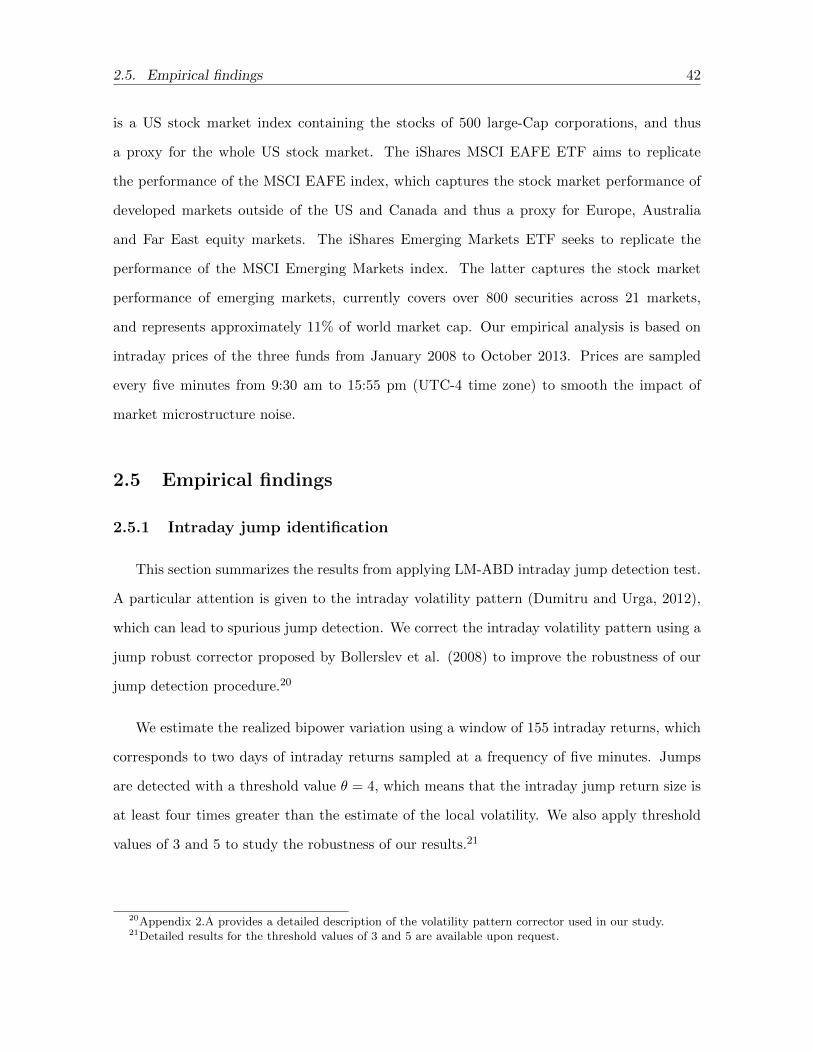
2.5. Empirical findings 42
is a US stock market index containing the stocks of 500 large-Cap corporations, and thus
a proxy for the whole US stock market. The iShares MSCI EAFE ETF aims to replicate
the performance of the MSCI EAFE index, which captures the stock market performance of
developed markets outside of the US and Canada and thus a proxy for Europe, Australia
and Far East equity markets. The iShares Emerging Markets ETF seeks to replicate the
performance of the MSCI Emerging Markets index. The latter captures the stock market
performance of emerging markets, currently covers over 800 securities across 21 markets,
and represents approximately 11% of world market cap. Our empirical analysis is based on
intraday prices of the three funds from January 2008 to October 2013. Prices are sampled
every five minutes from 9:30 am to 15:55 pm (UTC-4 time zone) to smooth the impact of
market microstructure noise.
2.5 Empirical findings
2.5.1 Intraday jump identification
This section summarizes the results from applying LM-ABD intraday jump detection test.
A particular attention is given to the intraday volatility pattern (Dumitru and Urga, 2012),
which can lead to spurious jump detection. We correct the intraday volatility pattern using a
jump robust corrector proposed by Bollerslev et al. (2008) to improve the robustness of our
jump detection procedure.20
We estimate the realized bipower variation using a window of 155 intraday returns, which
corresponds to two days of intraday returns sampled at a frequency of five minutes. Jumps
are detected with a threshold value θ = 4, which means that the intraday jump return size is
at least four times greater than the estimate of the local volatility. We also apply threshold
values of 3 and 5 to study the robustness of our results.21
20Appendix 2.A provides a detailed description of the volatility pattern corrector used in our study.21Detailed results for the threshold values of 3 and 5 are available upon request.

2.5. Empirical findings 43
Table 2.1: Summary statistics of jump occurrences, jump sizes and intraday returns.This table shows summary statistics of total and jump returns in Panels A and B, respectively. Jumpsstatistics include the total number of jumps, positive and negative jumps, mean, standard deviation,skewness and kurtosis of jump returns of the three ETFs including SPY, ETA, and EEM. The percent-age of positive jumps and negative jumps from all jumps are reported in brackets next to the numberof positive and negative jumps. Jumps are detected using the LM-ABD procedure with a critical valueθ = 4. See Section 2.2 for the detail of jump test statistics. The intraday prices of the three ETFsfrom January 2008 to October 2013 are included. Prices are sampled every five minutes from 9:30 amto 15:55 pm.
SPY EFA EEM
Panel A: Jumps statistics
Intraday jumps 1119 1114 1024
Positive jumps 475 (42%) 495 (44%) 455 (44%)
Negative jumps 644 (58%) 619 (56%) 569 (56%)
Mean of jump returns -4.3e-04 -2.5e-04 -2.1e-04
Std of jump returns 0.0048 0.0047 0.0058
Skewness of jump returns -0.59 0.27 -0.006
Kurtosis of jump returns 14.00 8.40 15.60
Panel B: Returns statistics
Mean of total returns 2.4e-06 4.7e-06 3.5e-06
Std of total returns 0.0014 0.0013 0.0017
Skewness of total returns -0.12 0.11 0.09
Kurtosis of total returns 36.66 24.40 38.33
Table 2.1 provides the number of total, positive and negative intraday jumps detected over
the study period. We identify 1119, 1114 and 1024 intraday jumps for SPY, EFA and EEM
funds respectively, or 0.989%, 0.986% and 0.900% of the total number of intraday returns.
The number of detected intraday jumps is higher in developed markets (US and EFA) than in
emerging markets, suggesting a higher degree of asset comovement within developed markets.
A positive (negative) jump is a jump with positive (negative) return. The results show that
the number of negative jumps is more than 56% of total number of detected jumps for each
fund. Stock markets thus tend to experience more price jumps when markets are bearish.
Table 2.1 also reveals that the mean of intraday jump returns of SPY (-4.3e-04) in absolute
value is two times higher than the one for EFA and EEM (-2.5e-04 and -2.1e-04, respectively).

2.5. Empirical findings 44
This result indicates that negative intraday price movements are larger for the US market.
However, the intraday jump return volatility is higher for emerging markets (0.0058) than for
developed ones (around 0.0047).
At a daily level, Table 2.2 shows that the percentage number of days with at least one
intraday jump is around 40% of the total number of days of the study period (1468 days).
The high proportion of jump days might be explained by a higher jump activity during the
financial crisis period. It is also related to the high level of sampling frequency (five minutes)
used in our paper.
Table 2.3 shows some statistics of detected cojumps. Over the study period, we find 585
cojumps between SPY and EFA funds, 509 cojumps between EEM and SPY funds, and 458
cojumps between EEM and EFA funds. This finding indicates that developed equity markets
are more linked to the US market than emerging markets. The three funds are involved in 365
cojumps, with the number of negative cojumps (61%) being higher than positive cojumps.
Table 2.2: Summary statistics of jump occurrences at day level.This table presents the number of days with no jumps, one jump, and two jumps up to more than 5jumps of the price of the three ETFs (SPY, EFA and EEM). The last row shows the percentage of dayswith at least one jump. Jumps are detected using LM-ABD procedure with a critical value θ = 4. SeeSection 2.2 for the detail of jump test statistics. The intraday prices of the three ETFs from January2008 to October 2013 are included. Prices are sampled every five minutes from 9:30 am to 15:55 pm.
SPY EFA EEM
0 843 843 879
1 357 365 353
2 139 147 128
3 75 50 60
4 30 37 26
5 12 13 9
More than 5 12 13 13
At least one jump 42% 42% 40%

2.5. Empirical findings 45
Table 2.3: Summary statistics of cojump occurrences.This table reports the number of total positive and negative detected cojumps among ETFs includingSPY and EFA (column 1), SPY and EEM (column 2), EFA and EEM (column 3) and SPY, EFAand EEM (column 4). The percentage of cojumps compared to the total number of detected jumps isshown in brackets next to intraday cojumps. Jumps are detected using the LM-ABD procedure witha critical value θ = 4. See Section 2.2 for the detail of jump and cojump identification procedure. Theintraday prices of the three ETFs from January 2008 to October 2013 are included. Prices are sampledevery five minutes from 9:30 am to 15:55 pm.
SPY / EFA SPY/EEM EFA/EEM SPY/EFA/EEM
Intraday cojumps 585 (53%) 509 (50%) 458 (45%) 365 (36%)
Positive cojumps 242 203 193 144
Negative cojumps 343 306 265 221
Table 2.4 shows the probability to have at least one cojump between SPY and EFA is 0.27
at the daily level. This probability is lower for SPY and EEM (0.23) and for EFA and EEM
(0.22). The probability that the three funds simultaneously experience a cojump is 0.18.
Table 2.4: Summary statistics of cojump occurrences at day level.This table presents the number of days with no cojumps, one cojump, two cojumps up to more thanfour cojumps among ETFs including SPY and EFA in column 2, SPY and EEM in column 3, EFAand EEM in column 4, and SPY, EFA, and EEM in column 5. The last row shows the percentage ofdays with at least one cojump. Jumps are detected using the LM-ABD procedure with a critical valueθ = 4. See Section 2.2 for jump and cojump identification procedure. The intraday prices of the threefunds are from January 2008 to October 2013. Prices are sampled every five minutes from 9:30 am to15:55 pm.
SPY/EFA SPY/EEM EFA/EEM SPY/EFA/EEM
0 1071 1130 1147 1208
1 282 233 233 193
2 70 61 57 39
3 27 28 19 20
4 12 11 6 5
More than 4 3 5 6 3
At least one cojump 27% 23% 22% 18%

2.5. Empirical findings 46
Table 2.5: Summary statistics of cojumps between EUR/USD exchange rate and international equityfunds.The number of detected cojumps between EUR/USD exchange rate and respectively SPY (row 2),EFA (row 3), EEM (row 4), SPY and EFA (row 5), SPY and EEM (row 6), EFA and EEM (row 7)are reported. The percentage of cojumps compared to the total number of detected jumps is shown inbrackets next to intraday cojumps. Jumps are detected using the LM-ABD procedure with a criticalvalue θ = 4. See Section 2.2 for jump and cojump identification procedure. The sample includes theintraday prices of the three ETFs from January 2008 to October 2013. Prices are sampled every fiveminutes from 9:30 am to 15:55 pm.
EUR/USD
SPY 162 (14.48%)
EFA 268 (24.06%)
EEM 162 (15.82%)
SPY/EFA 133 (11.94%)
SPY/EEM 110 (10.75%)
SPY/EFA/EEM 101 (9.86%)
We also examine if detected jumps and cojumps can be explained by exchange rates
movements. Table 2.5 reports the number of cojumps that involve EUR/USD exchange rate
with one or more of the three funds. We apply EUR and USD as they are the two major
currencies in the world. The probability of cojumps between the EUR/USD and EFA is the
highest (24%) whereas the probability of cojumps with SPY and EEM is respectively 14%
and 16%. The exposure to currency risk is relatively higher for EFA given that it is composed
largely of stocks that are quoted in EUR whereas the whole fund is traded in USD. The
probability that two or three funds jump at the same time as the EUR/USD exchange rate
remains less than 12%. These results suggest that only 12% of detected cojumps of three
funds are induced by exchange rate movements.
To examine the variation of the jump and cojump intensities over time, we calculate the
time-varying daily intensities of jumps (JI) and cojumps (CJI) using a rolling 6-month window
of observations as follows:
JI =
∑k
1Jumpik
Ndaysand CJI =
∑k
1Jumpik∩Jumpjk
Ndays

2.5. Empirical findings 47
2009 2010 2011 2012 2013 2014
0.2
0.4
0.6
0.8
1.0
1.2
1.4
Daily jump intensity
SPY
EFA
EEM
2009 2010 2011 2012 2013 2014
0.0
0.2
0.4
0.6
0.8
1.0
Daily cojump intensity
SPY and EFA
SPY and EEM
EFA and EEM
SPY , EFA and EEM
Figure 2.1: Jump and cojump occurrences.These figures show the variation of the daily jump and cojump intensities of the three funds (SPY, EFA,and EEM) from January 2008 to October 2013. The daily intensity of jumps (cojumps) is defined asthe daily average number of jumps (cojumps that involve two or three funds). These time-varying jumpintensities are calculated weekly using a rolling six-month window of observations. Prices are sampledevery five minutes from 9:30 am to 15:55 pm. Jumps are detected using the LM-ABD procedure witha critical value θ = 4. See Section 2.2 for jump and cojump identification procedure.

2.5. Empirical findings 48
where Ndays is the number of days of the observation period (120 business days in our case).
1Jumpikis an indicator function of jump occurrence for the ith asset at the intraday interval
k. 1Jumpik∩Jumpjkis an indicator function of cojump occurrence for the ith and jth assets at
the intraday interval k.
Figure 2.1 uncovers that the daily jump and cojump intensities have significantly increased
during the financial crisis of 2008-2009 for the three funds. There is a pattern that the US
market was the first to reach the peak of the jump intensity during the crisis followed by other
developed markets and then emerging markets, particularly during a peak in January 2010,
a drop in December 2010, and a jump in December 2012. The results support the evidence
in Ait-Sahalia et al. (2015). The cojump intensity is highest between funds of the US and
other developed markets, followed by funds of the US and emerging markets, and finally the
funds of other developed markets and emerging markets. The intensity of simultaneous jumps
of three funds is lowest. Overall, the lead/lag interaction of jumps is similar to pattern of
lead/lag during the financial crisis, i.e., the unusual increase of the intraday jumps seems to
be triggered in the US market and then propagated to the rest of the world.
2.5.2 Time and space clustering of intraday jumps
This section examines the dependencies between intraday jumps both within and across
markets. Figure 2.2 shows jumps in SPY tend to occur simultaneously with jumps in EFA
and EEM and their cojumps are clustered during the periods from June 21, 2010 to June 24,
2010 and August 23, 2010 to August 27, 2010. Thus, international intraday jumps are likely
to propagate both in time (in the same market) and in space (across markets).
We formally test jump propagation using the Hawkes process (Hawkes, 1971).22 This
process is a self-excited point process whose intensity depends on the path followed by the
point process and has been extensively used in different domains such as seismology and
neurology, but only recently in finance to model the dynamics of microstructure prices (Lee
22Note that this dependence pattern cannot be reproduced by the standard Poisson process, which assumesthe hypothesis of independence of the increments (jumps in our case) on disjoint time intervals.

2.5. Empirical findings 49
May Jun Jul Aug Sep Oct Nov
SPY
EFA
EEM
Figure 2.2: Time and space clustering of intraday jumps.This figure shows the arrival times of intraday jumps of the three funds from April 2010 to November2010. The intraday prices of the three ETFs including SPY, EFA, and EEM are included. Prices aresampled every five minutes from 9:30 am to 15:55 pm.
and Seo, 2017), trading activity, and asset jumps in financial markets (Ait-Sahalia et al., 2015;
Bormetti et al., 2015). For example, Ait-Sahalia et al. (2015) use a multivariate Hawkes jump-
diffusion model to investigate the financial contagion in the international equity markets at
daily level. Bormetti et al. (2015) employ high frequency data and the Hawkes processes to
reproduce the time clustering of jumps for 20 high-cap Italian stocks.
The univariate Hawkes process we use to capture the time clustering of intraday jumps
for each of the ETFs is given by:
dλt = β(λ∞ − λt)dt+ αdNt (2.20)
where Nt is the number of jumps occurring in the time interval [0, t]. A jump occurrence at
a given time will increase the intensity or the probability of another jump (self excitation).
The intensity increases by α whenever a jump occurs, and then decays back towards a level
λ∞ at a speed β. These parameters can be estimated using the maximum likelihood method.

2.5. Empirical findings 50
Given the jump arrival times t1, t2, . . . , tq, the likelihood function is written as:23
L(t1, t2, . . . , tq) = −λ∞tq +
q∑i=1
α
β
(e−β(tq−ti)
)+
q∑i=1
log (λ∞ + αA(i)) (2.21)
where A(i) =∑
tj<tie−β(ti−tj) for i ≥ 2 and A(1) = 0.
The univariate Hawkes process can be extended so that it captures the time and space
clustering of intraday jumps between n markets, such as:
dλi,t = βi(λi,∞ − λi,t)dt+n∑j=1
αi,jdNj,t, i = 1, . . . , n (2.22)
Under this model, a jump in market j increases not only the jump intensity within the
same market through αj,j (self excitation) but also the cross-market jump intensity through
αi,j (cross excitation). αj,j implies a degree where jumps are re-created within the same
market whereas αi,j suggests the propagation rate of jumps from market j to market i. The
jump intensity of market i reverts exponentially to its average level λi,∞ at a speed βi. Since
the numerical resolution of the trivariate Hawkes model for three ETFs is problematic owing
to the large number of parameters to be estimated, we limit the calibration procedure to
the bivariate model whereby the vector of unknown parameters only contains 8 parameters,
Θ = (λ1,∞, λ2,∞, β1, β2, α1,1, α1,2, α2,1, α2,2), as follows:
dλ1,t = β1(λ1,∞ − λ1,t)dt+ α1,1dN1,t + α1,2dN2,t
dλ2,t = β2(λ2,∞ − λ2,t)dt+ α2,1dN1,t + α2,2dN2,t
(2.23)
Panels A, B and C of Table 2.6 show the estimation results of the bivariate Hawkes
model for SPY/EFA, SPY/EEM and EFA/EEM, respectively. All the model parameters are
significant at conventional levels, implying that the bivariate Hawkes model satisfactorily fits
the data of intraday jump occurrences of three funds.
23See Ogata (1978) and Ozaki (1979) for the details of the maximum likelihood estimation.

2.5. Empirical findings 51
Table 2.6: Maximum likelihood estimation of the bivariate Hawkes model.The table below shows the results of the maximum likelihood estimation of the bivariate Hawkes modelfor pairs of ETFs including SPY/EFA (panel A), SPY/EEM (panel B) and EFA/EEM (panel C). SeeSection 2.5.2 for the detail of Hawkes process. The sample includes the intraday prices of the threeETFs from January 2008 to October 2013. Prices are sampled every five minutes from 9:30 am to 15:55pm. The values of the estimate, standard error, z- statistic and p-value are reported for each parameterof the bivariate model. ***, **, and * represent 0.1 percent, 1 percent and 5 percent significance levels,respectively.
Panel A: SPY/EFA
Estimate Std. Error z value Pr(z)
λspy,∞ 1.6305e-03 6.4929e-05 25.1122 <2.2 e-16***
λefa,∞ 1.5445e-03 6.4217e-05 24.0505 <2.2 e-16 ***
βspy 4.2957e-02 5.2288e-03 8.2154 <2.2 e-16 ***
βefa 1.9230e-02 1.6585e-03 11.5942 <2.2 e-16 ***
αspy,spy 1.2004e-02 1.8520e-03 6.4816 9.074 e-11 ***
αspy,efa 1.7864e-03 5.5554e-04 3.2156 0.001302 **
αefa,efa 3.7166e-03 4.9845e-04 7.4563 8.896 e-14 ***
αefa,spy 2.4015e-03 4.6676e-04 5.1452 2.673 e-07 ***
Panel B: SPY/EEM
Estimate Std. Error z value Pr(z)
λspy,∞ 1.5452e-03 6.4580e-05 23.9268 <2.2 e-16***
λeem,∞ 1.4443e-03 6.3741e-05 22.6583 <2.2 e-16 ***
βspy 1.8364e-02 1.6053e-03 11.4395 <2.2 e-16 ***
βeem 1.8342e-02 1.6588e-03 11.0573 <2.2 e-16 ***
αspy,spy 4.0540e-03 5.3480e-04 7.5804 3.445 e-14***
αspy,eem 2.1598e-03 4.6120e-04 4.6829 2.828 e-06 ***
αeem,eem 3.8814e-03 5.5318e-04 7.0164 2.277 e-12 ***
αeem,spy 2.2278e-03 4.2694e-04 5.2181 1.808 e-07 ***
Panel C: EFA/EEM
Estimate Std. Error z value Pr(z)
λefa,∞ 1.5471e-03 6.2625e-05 24.7045 <2.2 e-16***
λeem,∞ 1.4194e-03 6.2419e-05 22.7400 <2.2 e-16 ***
βefa 2.6309e-02 2.7030e-03 9.7335 <2.2 e-16 ***
βeem 2.5798e-02 2.7876e-03 9.2544 <2.2 e-16 ***
αefa,efa 4.0065e-03 5.2480e-04 7.6342 2.272 e-14 ***
αefa,eem 2.1582e-03 4.7037e-04 4.5882 4.470 e-06 ***

2.5. Empirical findings 52
αeem,eem 3.7661e-03 5.5861e-04 6.7418 1.564 e-11 ***
αeem,efa 2.5773e-03 4.4460e-04 5.7969 6.754 e-09 ***
The large value of the parameters α1,1 and α2,2 provides clear evidence that intraday
jumps of the US market, other developed markets and emerging markets are strongly recre-
ated within individual market. Panel A indicates that the self-excitation activity for the US
market is higher than that of other developed markets. Compared to emerging markets, the
self-excitation activity for the US (Panel B) and for the other developed market (Panel C)
is greater. The higher degree of market efficiency in the US and other developed market
might explain their high level of self-excitation activity. On the other hand, the value of the
parameters α1,2 and α2,1, which measure the degree of jump transmission between markets, is
smaller than the self-excitation parameters. The degree of jump transmission between markets
is asymmetric with a stronger transmission from the US market to other developed markets
(αefa,spy = 2.40 e-03) than from the US market to emerging markets (αeem,spy = 2.23 e-03).
The transmission of jumps in the other way around is also significant but the strength is
weaker. The emerging markets receive more jump spillover from the other developed markets
than what they transmit to other markets.
2.5.3 Cojumps and optimal portfolio composition
We now examine the effect of cojumps on the optimal portfolio composition within the
mean-variance and mean-CVaR frameworks from the US investor perspective. More precisely,
we study how the demand of foreign assets varies with cojumps between domestic and foreign
assets. The portfolio we consider is composed of one domestic asset (represented by the SPY
fund) and two foreign assets (represented by EFA and EEM funds). All funds are expressed
from the US investor’s perspective and thus in USD. Assets weights can be negative, meaning
that the domestic investor can take short position on the domestic and foreign assets. The
demand of foreign assets is defined as the sum of optimal allocation weights of EFA and EEM
funds resulting from our portfolio optimization procedure based on daily historical returns

2.5. Empirical findings 53
(1469 observations for each fund) and the variance and CVaR approaches. The portfolio
optimization is performed each week using a rolling window of about 120 daily returns (6
months) that immediately precede the optimization day. We also consider different rolling
window sizes (3, 9, 12, 15 and 18 months), and the results remain intact.24
2009 2010 2011 2012 2013 2014
−2
−1
01
Variance
CVaR
Figure 2.3: The variation of the optimal proportion of foreign assets.This figure shows the variation of the optimal proportion of the foreign assets (EFA and EEM) obtainedfrom variance and CVaR minimization approaches. The optimal portfolio composition is determinedin a monthly basis, using a rolling six-month window of daily returns. The portfolio is composed ofone domestic asset (SPY) and two foreign assets (EFA and EEM).
Our optimization problem consists of minimizing the portfolio risk (standard deviation
or CVaR) under the budget’s constraint of weights summing to one. Figure 2.3 shows the
dynamic changes in the optimal proportion of the foreign assets (EFA and EEM) for variance
and CVaR approaches. Both approaches lead to similar portfolio compositions over the study
period, but the minimum CVaR portfolio composition is more volatile than the minimum
variance portfolio. This might be because CVaR is determined using few extreme observations
in the lower tail of the returns distribution whereas the variance takes into account all available
observations. Panels A and B of Figure 2.4 show that the standard deviation and CVaR are
varying in a similar fashion over time. Moreover, the risk of the domestic market (SPY fund)
is often lower than that of foreign markets (EFA and EEM funds), regardless of the risk
measures. This might be because from domestic market perspective (here is the US), the
foreign market is subject to the variability of both foreign stock market and exchange rate.
24Detailed results for different rolling window sizes (3, 9, 12, 15 and 18 months) are available upon request.

2.5. Empirical findings 54
Panels C, D and F of Figure 2.4 show respectively the variation of the daily return correlation,
the realized correlation and realized correlation of SPY/EFA jumps, SPY/EEM jumps and
EFA/EEM jumps.25 The graphs suggest that three correlation measures are closely linked
to each other. In other words, correlated jumps have similar pattern of comovement to both
correlated daily and intraday returns. The correlation of jumps is relatively high over the
period of study. It varies between 0.6 and 1 for three pairs of funds. The jump correlation is
thus significant and positively high.26 On average, the correlation between SPY/EFA jumps
is the highest. It is then followed by SPY/EMM and EFA/EEM jumps.
As the composition of the optimal portfolio becomes available, we are able to study how
cojumps between domestic and foreign markets affect the portfolio composition. We hypothe-
size that a high intensity of cojumps between domestic and foreign markets leads to a decrease
in benefit from diversifying internationally and thus foreign asset holding. We begin our anal-
ysis with the calculation of the correlation between the daily intensity of cojumps and the
optimal proportion of foreign assets that we obtained with variance and CVaR approaches.
Although our exercise onward has the US as home market and the rest as foreign markets,
our analysis can be generalized to any home and host markets with respect to our theoretical
framework in Section 2.3.1, provided that the variability of home market is lower than the
variability of host markets.
The main results for the variance approach, summarized in Table 2.7, show a negative
correlation between the demand of foreign assets and the daily intensity of cojumps between
the domestic market (SPY fund) and each of foreign markets (EFA and EEM funds).27We
find a correlation of -0.10 for SPY/EFA cojumps intensity and -0.20 for SPY/EEM cojumps
intensity with foreign asset holding. When we consider the cojumps that involve the three
funds, we find a negative correlation of -0.19. We get similar results for positive and negative
25The daily correlation is the standard correlation coefficient calculated monthly using a rolling six-monthwindow of daily returns. The realized total and jump correlations are estimated monthly using a rollingsix-month window of intraday returns.
26Refer to Jacod and Todorov (2009) for more details about the accuracy of the jump correlation estimator.27We find similar results for the CVaR approach. Detailed results are not presented due to limited space
but are available upon request.

2.5. Empirical findings 55
Panel A: Standard deviation of SPY, EFA and EEM
2009 2010 2011 2012 2013 2014
0.0
00
.02
0.0
40
.06
0.0
8
SPY
EFA
EEM
Panel B: CVaR of SPY, EFA and EEM
2009 2010 2011 2012 2013 2014
0.0
00
.05
0.1
00
.15
SPY
EFA
EEM
Figure 2.4: Standard deviation, CVaR and correlations of domestic and foreign assets.These figures show the variation of the standard deviation, CVaR and the correlation, respectivelyof SPY, EFA and EEM. Panels A and B present moving standard deviation and absolute value ofthe CVaR, respectively of SPY, EFA and EEM. Panel C presents the time-varying correlation ofrespectively SPY and EFA, SPY and EEM and EFA and EEM. These variations are calculated monthlyfor a rolling six-month window of daily returns. The panels D and E represent the variation of therealized correlation and the realized jump correlation, of respectively SPY and EFA, SPY and EEMand EFA and EEM. The realized correlations are calculated monthly for a rolling six-month window ofintraday returns. The intraday prices of the three ETFs including SPY, EFA, and EEM from January2008 to October 2013 are included. Prices are sampled every five minutes from 9:30 am to 15:55 pm.
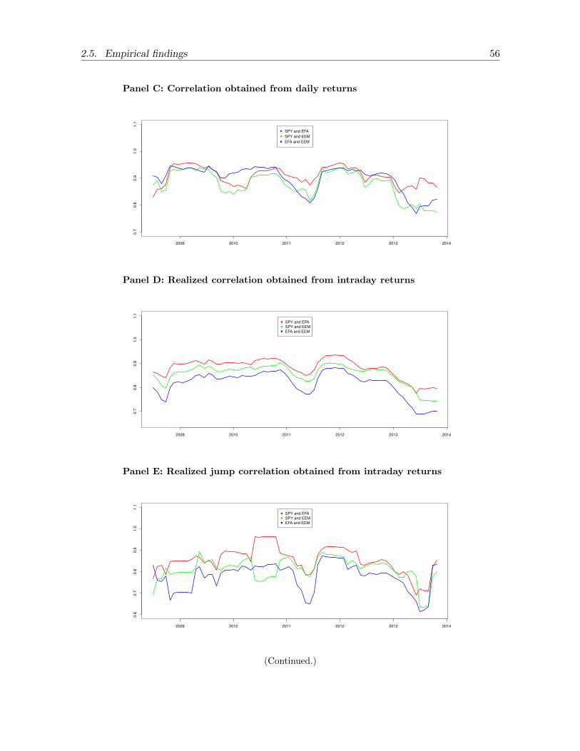
2.5. Empirical findings 56
Panel C: Correlation obtained from daily returns
2009 2010 2011 2012 2013 2014
0.7
0.8
0.9
1.0
1.1
SPY and EFA
SPY and EEM
EFA and EEM
Panel D: Realized correlation obtained from intraday returns
2009 2010 2011 2012 2013 2014
0.7
0.8
0.9
1.0
1.1
SPY and EFA
SPY and EEM
EFA and EEM
Panel E: Realized jump correlation obtained from intraday returns
2009 2010 2011 2012 2013 2014
0.6
0.7
0.8
0.9
1.0
1.1
SPY and EFA
SPY and EEM
EFA and EEM
(Continued.)

2.5. Empirical findings 57
cojumps except for positive cojump between SPY/EFA where the correlation with foreign
asset holding is not significant. This result implies that, regardless of the sign of returns,
investors do not like cojumps between domestic and foreign assets.
In addition to cojumps intensity, we find that the negative relation between correlated
jumps and foreign holdings is more pronounced. The measure of jump correlation is shown
analytically in Section 2.3.1. It is more appropriate in practice to use the jump correlation to
measure the degree of linkage between assets jumps. Contrary to cojump intensity measure,
which only takes into account the frequency effect, the jump correlation captures both the
jump frequency and size effects. It thus provides a more accurate measure of the degree
of jump comovement than the cojump intensity. We find a strong negative correlation of
-0.56 for SPY/EFA correlated jumps and -0.39 for SPY/EEM correlated jumps. Negative
and positive jump correlations are also negatively correlated to foreign asset holdings. The
correlation between foreign assets holdings and correlated jumps is higher for the portfolio of
SPY and EFA funds than for the portfolio of SPY and EEM funds. This is expected given
that the US market has a higher correlation with the other developed ones. We also examine
if our results are sensitive to exchange rate jump risk. We exclude all assets jumps that occur
simultaneously with EUR/USD exchange rate jumps and repeat the analysis. The significant
negative link between jump correlation and the demand of foreign assets remains intact. We
find a correlation of -0.50 for SPY/EFA and -0.38 for SPY/EEM.28
In Table 2.8, we examine the correlation between foreign asset holdings and idiosyncratic
jumps where idiosyncratic jumps are defined earlier as jumps that occur in a single market.
Specifically, we measure the correlation between the daily intensity of idiosyncratic jumps (of
respectively SPY, EFA and EEM funds) and the optimal proportion of foreign assets and find
a positive correlation for SPY (0.45), EFA (0.35) and EEM (0.40). In contrast to systematic
jumps, idiosyncratic jumps increase foreign holdings. That is, investors seem to be aware that
holding more foreign assets in their portfolios help them diversify idiosyncratic jump risks.
28Detailed results of the correlation between foreign asset holdings and correlated jumps are not presentedfor brevity. They are available upon request.

2.5. Empirical findings 58
Table 2.7: Correlation between the daily intensity of cojumps and the optimal proportion of the foreignassets.This table presents the correlation between the daily intensity of cojumps and the optimal proportionof the foreign assets (the sum of optimal weights of EFA and EEM) calculated using the varianceminimization approach. Panel A shows the results for all cojumps; Panel B shows the results ofcojumps that occur independently of EUR/USD exchange rate jumps. The daily intensity of cojumpsis defined as the daily average number of cojumps that involve two or three funds and determined weeklyusing a six-month rolling window of observations. Positive and negative implies cojumps of positiveand negative returns, respectively. See Section 2.2 for jump and cojump identification procedure,and Section 2.5.3 for the estimation of the optimal foreign assets holdings. The sample includes theintraday prices of the three funds from January 2008 to October 2013. Prices are sampled every fiveminutes from 9:30 am to 15:55 pm. ***, **, and * represent 0.1 percent, 1 percent and 5 percentsignificance levels, respectively.
Panel A: All cojumps
Assets used to estimate
the intensity of cojumps Estimate (Correlation) Confidence interval (95%) T-stat P-value
SPY and EFA -0.10 [-0.21, -0.02] -1.56 0.11
Positive SPY and EFA 0.006 [-0.11, 0.13] 0.10 0.92
Negative SPY and EFA -0.15 [-0.26, -0.03] -2.48 0.014*
SPY and EEM -0.20 [-0.31, -0.08] -3.24 0.001**
Positive SPY and EEM -0.15 [-0.26, -0.03] -2.50 0.013*
Negative SPY and EEM -0.16 [-0.27, -0.04] -2.48 0.014*
SPY, EFA and EEM -0.19 [-0.30, -0.07] -3.13 0.002**
Positive SPY, EFA and EEM -0.18 [-0.30, -0.07] -3.06 0.002**
Negative SPY, EFA and EEM -0.13 [-0.24, -0.01] -2.12 0.034*
Panel B: Excluding cojumps that occur simultaneously with EUR and USD exchange rate jump
Assets used to estimate
the intensity of cojumps Estimate (Correlation) Confidence interval (95%) T-stat P-value
SPY and EFA 0.05 [-0.07, 0.16] 0.75 0.45
Positive SPY and EFA -0.05 [-0.17, 0.07] -0.78 0.44
Negative SPY and EFA 0.09 [-0.03, 0.21] 1.50 0.13
SPY and EEM -0.14 [-0.26, -0.02] -2.37 0.02*
Positive SPY and EEM -0.18 [-0.30, -0.06] -2.97 0.003**
Negative SPY and EEM -0.06 [-0.18, 0.06] -0.99 0.32
SPY, EFA and EEM -0.16 [-0.27, -0.04] -2.66 0.008**
Positive SPY, EFA and EEM -0.27 [-0.38, -0.16] -4.62 5.85 e-06***
Negative SPY, EFA and EEM -0.01 [-0.13,0.10] -0.22 0.82

2.5. Empirical findings 59
Table 2.8: Correlation between the daily intensity of idiosyncratic jumps and the demand of foreignassets.This table presents the correlation between the daily intensity of idiosyncratic jumps and the optimalproportion of foreign assets (the sum of optimal weights of EFA and EEM) calculated using the varianceminimization approach. The daily intensity of idiosyncratic jumps is defined as the daily averagenumber of jumps that involve only one fund and determined weekly using a six-month rolling windowof observations. See Section 2.2 for the detail of jump test statistics and definition of idiosyncraticjumps, and Section 2.5.3 for the estimation of the optimal foreign assets holdings. The sample includesthe intraday prices of the three funds from January 2008 to October 2013. Prices are sampled everyfive minutes from 9:30 am to 15:55 pm. ***, **, and * represent 0.1 percent, 1 percent and 5 percentsignificance levels, respectively.
Assets used to estimate
the intensity of idiosyncratic jumps Estimate (Correlation) Confidence interval (95%) T-stat P-value
SPY 0.45 [0.35, 0.54] 8.21 9.10e-15***
EFA 0.35 [0.24, 0.45] 6.15 2.76e-09***
EEM 0.40 [0.29, 0.50] 7.10 1.15e-11***
Finally, we examine how higher-order moments induced by idiosyncratic and systematic
jumps affect the optimal portfolio composition. For this purpose, we compare the optimal
portfolio weights for an investor who recognizes idiosyncratic and systematic jumps and an-
other investor who ignores them and assumes a pure multivariate diffusion process for asset
returns. Both investors have the same CRRA utility function and select their portfolio compo-
sitions based on one domestic asset (SPY) and two foreign assets (EFA and EEM). The port-
folio optimization is performed yearly following the methodology described in Section 2.3.2.
The optimal weights are obtained by resolving numerically Eq. 2.19. The risk aversion co-
efficient is set to three and the risk-free rate to zero. The parameters of the multivariate
jump-diffusion process are estimated on a yearly basis using intraday returns of the preceding
year. Table 2.9 reports the detail of jump-diffusion model estimation over the whole period.
The results in Table 2.10 show that optimal domestic asset weights are almost the same for
the pure-diffusion and jump-diffusion investors. The impact of jump higher-order moments
on the optimal portfolio composition is thus insignificant.29 This finding is consistent with
29The ratioµt1s
t1
(vt1)2, defined in Section 2.3.2, is in the order of 10e-4 (<< 1) for three funds, which explains
the insignificant impact of higher-order moments.

2.5. Empirical findings 60
Das and Uppal (2004) who find similar results for systemic jumps.30 That is, the difference
between the portfolio composition of an investor who cares about systemic jumps and another
investor who ignores them is small.
Taken together, the findings in this section show that the jump correlation, which is
the normalized second joint moment of jump returns, reduces foreign asset holdings in in-
ternational portfolios, whereas higher-order moments have no significant effect on portfolio
composition.
Table 2.9: Multivariate jump-diffusion model estimation.The tables report the results of the estimation of the multivariate jump-diffusion model introducedin Section 2.3.2. The estimation is performed using intraday prices of the three funds from January2008 to October 2013. Prices are sampled every five minutes from 9:30 am to 15:55 pm. Jumps andcojumps are detected using the methodology defined in Section 2.2.
SPY EFA EEM
µi 6.8e-06 7.4e-06 5.8e-06
µsys,upi 0.00472 0.00475 0.00563
µsys,downi -0.00417 -0.00426 -0.00471
µid,upi 0.00328 0.00344 0.00410
µid,downi -0.00312 -0.00308 -0.00363
νsys,upi 0.00354 0.00312 0.00467
νsys,downi 0.00375 0.00324 0.00357
νid,upi 0.00291 0.00319 0.00395
νid,downi 0.00310 0.00225 0.00375
λsys,up 0.00127 0.00127 0.00127
λsys,down 0.00196 0.00196 0.00196
λid,upi 0.00293 0.00310 0.00274
λid,downi 0.00373 0.00352 0.00308
ρi,jσiσji,j SPY EFA EEM
SPY 1.7e-06
EFA 1.5e-06 1.5e-06
EEM 1.9e-06 1.7e-06 2.5e-06
30Systemic jumps are defined as infrequent, large and highly correlated jumps.

2.5. Empirical findings 61
Table 2.10: Optimal portfolio weights using power utility maximization approach.The table reports the optimal weight of the domestic asset (SPY fund) for a jump-diffusion investorwho accounts for idiosyncratic and systematic jumps and another pure-diffusion investor who ignoresthem. The portfolio optimization is performed yearly using intraday returns of the preceding year.The risk aversion coefficient is set to three and the riskless asset weight to zero. The multivariatejump-diffusion model and the power utility optimization problem are introduced in Section 2.3.2.Jumps and cojumps are detected using the methodology defined in Section 2.2.
pure-diffusion jump-diffusion
2008 -1.31 -1.33
2009 -2.40 -2.41
2010 1.89 1.91
2011 1.69 1.64
2012 0.25 0.25
2013 -0.76 -0.76
2.5.4 Cojumps and the benefits of international portfolio diversification
The results of the Section 2.5.3 show that cojumps in international equity markets are an
indirect barrier to the holding of foreign assets. To the extent that they amplify the level of
equity market comovement, it is expected that they negatively affect the benefits of portfolio
diversification. We confirm this by examining the link between the number of cojumps and
the measure of international diversification benefits in the spirit of Christoffersen et al. (2012)
proposing to measure the conditional diversification benefit (CDB) as follows:
CDBβ(w) =φβ − φβ(w)
φβ − αβ(w)(2.24)
where αβ(w) and φβ(w) are the values of the VaR and the CVaR of the portfolio loss function
associated with the vector of weights w and the confidence level β.31 By construction, the
αβ(w) refers to the lower bound of the portfolio’s expected shortfall, while φβ is the upper
bound of the portfolio’s expected shortfall and is defined as the weighted average of the
individual assets’ CVaRs (φβ,i):
φβ =
n∑i=1
wiφβ,i (2.25)
31See Appendix 2.B for more details about the VaR and the CVaR of the portfolio loss function.
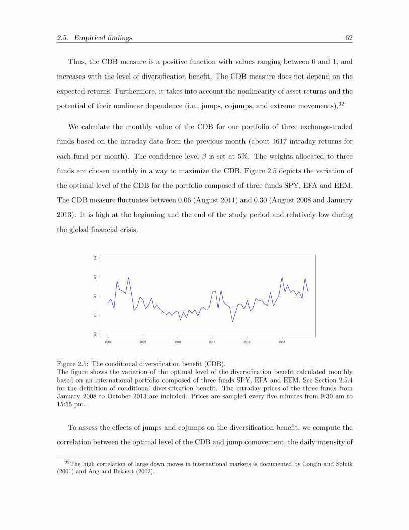
2.5. Empirical findings 62
Thus, the CDB measure is a positive function with values ranging between 0 and 1, and
increases with the level of diversification benefit. The CDB measure does not depend on the
expected returns. Furthermore, it takes into account the nonlinearity of asset returns and the
potential of their nonlinear dependence (i.e., jumps, cojumps, and extreme movements).32
We calculate the monthly value of the CDB for our portfolio of three exchange-traded
funds based on the intraday data from the previous month (about 1617 intraday returns for
each fund per month). The confidence level β is set at 5%. The weights allocated to three
funds are chosen monthly in a way to maximize the CDB. Figure 2.5 depicts the variation of
the optimal level of the CDB for the portfolio composed of three funds SPY, EFA and EEM.
The CDB measure fluctuates between 0.06 (August 2011) and 0.30 (August 2008 and January
2013). It is high at the beginning and the end of the study period and relatively low during
the global financial crisis.
2008 2009 2010 2011 2012 2013
0.0
0.1
0.2
0.3
0.4
Figure 2.5: The conditional diversification benefit (CDB).The figure shows the variation of the optimal level of the diversification benefit calculated monthlybased on an international portfolio composed of three funds SPY, EFA and EEM. See Section 2.5.4for the definition of conditional diversification benefit. The intraday prices of the three funds fromJanuary 2008 to October 2013 are included. Prices are sampled every five minutes from 9:30 am to15:55 pm.
To assess the effects of jumps and cojumps on the diversification benefit, we compute the
correlation between the optimal level of the CDB and jump comovement, the daily intensity of
32The high correlation of large down moves in international markets is documented by Longin and Solnik(2001) and Ang and Bekaert (2002).

2.5. Empirical findings 63
cojumps and idiosyncratic jumps, both calculated on a monthly basis from the cojumps and
jumps detected from the previous month. The daily intensity of cojumps refers to the daily
average number of cojumps involving three funds, while the daily intensity of idiosyncratic
jumps refers to the daily average number of jumps involving only one fund. We also consider
the correlation between the optimal level of CDB and jump comovement.33 The latter is the
monthly average jump correlation of three funds, computed from the previous month intraday
data.
The findings in Table 2.11 show that the CDB is negatively correlated with cojumps in-
tensity (-0.37) and correlated jumps (-0.65). In contrast, the CDB is positively correlated
with idiosyncratic jumps intensity (0.40). The strong negative dependence between the di-
versification benefit and jump comovement is also shown in Figure 2.6. Taken together, these
results indicate that the international diversification benefit increases with the intensity of
idiosyncratic jumps and decreases with the level and intensity of cojumps observed in the in-
ternational markets. They further confirm our previous findings that domestic (US) investors
allocate more money towards home assets in the presence of cojumps between US and foreign
markets.
Table 2.11: The impact of simultaneous and idiosyncratic jumps on the optimal level of the diversifi-cation benefit.The table reports the measures of correlation between the conditional diversification benefit (CDB)and correlated jumps, daily cojumps intensity and daily idiosyncratic jumps intensity, respectively.The diversification benefit is defined in Section 2.5.4. The CDB is computed monthly from the pre-vious month intraday data. The correlation of jumps is the average correlation of jumps among thethree ETFs including SPY, EFA, and EEM calculated on a monthly basis from the previous monthintraday data. See Equations (2.12) to (2.14) for correlated jumps estimation. The daily intensity ofcojumps is computed on a monthly basis as the daily average number of cojumps that involve threefunds detected from the previous month. The daily intensity of idiosyncratic jumps is measured on amonthly basis as the average daily number of jumps that involve only one market. See Section 2.2 forjump and cojump identification procedure. The intraday prices of the three funds from January 2008to October 2013 are included. Prices are sampled every five minutes from 9:30 am to 15:55 pm.
Correlation Estimate (Correlation) Confidence interval (95%) T-stat P-value
Correlated jumps and CDB -0.65 [-0.77, -0.49] -7.05 1.1e-09***
Cojumps intensity and CDB -0.37 [-0.56, -0.15] -3.3 0.0015**
Idiosyncratic jumps intensity and CDB 0.40 [0.18, 0.58] 3.61 0.0005***
33The jump correlation measure has been introduced in Section 2.3.1.

2.6. Conclusion 64
0.6 0.7 0.8 0.9
0.1
00
.15
0.2
00
.25
0.3
0
Correlation of jumps
Op
tim
al C
DB
Figure 2.6: Linear regression between the conditional diversification benefit (CDB) and the correlationof jumps.The figure displays a scatterplot with a regression line showing the linear relationship between theoptimal level of the conditional diversification benefit and jump correlation. Diversification benefit isdefined in Section 2.5.4. Jump correlation is the average correlation of jumps from different pairs ofthe three ETFs including SPY, EFA, and EEM computed on a monthly basis. Jump correlation isdefined in Section 2.3.1. The intraday prices of the three funds from January 2008 to October 2013are included. Prices are sampled every five minutes from 9:30 am to 15:55 pm.
2.6 Conclusion
In this paper, we investigate how jumps and cojumps in international equity markets af-
fect international asset allocation and diversification benefits. Using a nonparametric intraday
jump detection technique developed by Lee and Mykland (2008) and Anderson et al. (2007)
and intraday data from three international exchange-traded funds as proxies for international
equity markets, we find that intraday jumps are transmitted both in time (in the same mar-
ket) and in space (across markets). The markets under consideration also have tendency to
be involved in cojumps. The high and significant degree of jumps synchronization in interna-
tional equity markets suggests that the jump risk is rather systematic and thus could not be
eliminated through the diversification.
We study the impact of cojumps on optimal international portfolio based on portfolio
variance and CVaR minimisation approaches and find a negative link between the demand
for foreign assets and cojumps between domestic and foreign markets. This result implies

2.6. Conclusion 65
that a domestic investor will invest less in foreign markets when the frequency and size of
cojumps between domestic and foreign assets increase. We also find the negative link between
the intensity of cojumps and the conditional diversification benefit measure suggested by
Christoffersen et al. (2012). Putting differently, the high jump correlation increases the cross-
market comovement, and therefore reduces the international diversification benefit and leads
investors to prefer home assets. In contrast, we find that idiosyncratic jumps have a positive
effect on foreign asset holding and diversification benefits. Finally, the impact of higher-order
moments induced by idiosyncratic and systematic jumps on optimal international portfolio
composition is insignificant.
This work opens interesting avenues for future research. It would be of great interest to
broaden the scope of this study by including a larger number of international equity indices
and examining the impact of asset cojumps on the demand for foreign assets for a larger panel
of countries. Studying the underlying mechanisms of cojumps in international equity markets
should also be of interest.

References
Ait-Sahalia, Y., Cacho-Diaz, J., and Laeven, R., 2015. Modeling financial contagion using
mutually exciting jump processes. Journal of Financial Economics 117, 585-606.
Aıt-Sahalia, Y., Xiu, D., 2016. Increased correlation among asset classes: Are volatility or
jumps to blame, or both? Journal of Econometrics 194, 205-219.
Andersen, T.G, Bollerslev, T., and Dobrev, D., 2007. No-arbitrage semi-martingale restric-
tions for continuous-time volatility models subject to leverage effects, jumps and i.i.d. noise:
Theory and testable distributional implications. Journal of Econometrics 138 (1), 125-180.
Andersen, T.G., Dobrev, D., and Schaumburg, E, 2012. Jump robust volatility estimation
using nearest neighbor truncation. Journal of Econometrics 169 (1), 74-93.
Ang, A., and Bekaert, G., 2002. International Asset Allocation with Regime Shifts, Review
of Financial Studies 15, 1137-1187.
Artzner, P., Delbaen, F., Eber, J.M., Heath, D., 1997. Thinking coherently. Risk 10, 68-71.
Artzner, P., Delbaen, F., Eber, J., and Heath, D., 1999. Coherent measures of risk, Mathe-
matical Finance 9, 203-228.
Bae, K.H., Karolyi, G.A., and Stulz, R., 2003. A new approach to measuring financial conta-
gion. Review of Financial Studies 16, 717-763.
Barndorff-Nielsen O. E. and Shephard, N., 2004. Power and bipower variation with stochastic
volatility and jumps. Journal of Financial Econometrics 2, 1-37.
Barndorff-Nielsen, O. E. and Shephard, N., 2006a. Econometrics of testing for jumps in fi-
nancial economics using bipower variation. Journal of Financial Econometrics 4, 1-30.
Barndorff-Nielsen OE, Shephard N. 2006b. Measuring the impact of jumps on multivariate
price processes using bipower covariation. Manuscript.
66

REFERENCES 67
Basak, S. and Shapiro, A., 2001. Value-at-risk based risk management: Optimal policies and
asset prices. Review of Financial Studies 14, 371-405.
Bekaert, G., Erb, C., Harvey, C., Viskanta, T., 1998. The distributional characteristics of
emerging market returns and asset allocation. Journal of Portfolio Management 24 (2),
102- 116.
Bollerslev, T., Law, T. H., Tauchen, G., 2008. Risk, jumps, and diversification. Journal of
Econometrics 144 (1), 234-256.
Bollerslev, T., and Todorov, V., 2011. Tails, fears, and risk premia. Journal of Finance 66 (6),
2165-2211.
Bormetti, G., Calcagnile, L.M., Treccani, M., Corsi, F., Marmi, S., Lillo, F., 2015. Modelling
systemic price cojumps with hawkes factor models. Quantitative Finance 15, 1137-1156.
Branger, N., Muck, M., Seifried, F.T., and Weisheit, S., 2017. Optimal portfolios when vari-
ances and covariances can jump. Journal of Economic Dynamics and Control 85, 59-89.
Choi, N., Fedenia, M., Skiba, H., Sokolyk, T., 2017. Portfolio concentration and performance
of institutional investors worldwide. Journal of Financial Economics 123 (1), 189-208.
Christensen, K., Oomen, R., and Podolskij, M., 2014. Fact or friction: Jumps at ultra high
frequency. Journal of Financial Economics114 (3), 576-599.
Christoffersen, P., Errunza, V., Langlois, H., and Jacobs, K., 2012. Is the Potential for Inter-
national Diversification Disappearing? Review of Financial Studies 25, 3711-3751
Corsi, F., Pirino, D., and Reno, R., 2010. Threshold bipower variation and the impact of
jumps on volatility forecasting. Journal of Econometrics 159, 276-288.
Das, S., Uppal, R., 2004. Systemic Risk and International portfolio choice. Journal of Finance
59, 2809-2834.

REFERENCES 68
Dumitru, A.M. and Urga, G., 2012. Identifying jumps in financial assets: A comparison
between nonparametric jump tests. Journal of Business & Economic Statistics 30 (2), 242-
255.
Dungey, M., McKenzie, M., and Smith, V., 2009. Empirical evidence on jumps in the term
structure of the US treasury market. Journal of Empirical Finance 16 (3), 430-445.
Dungey, M., Hvozdyk, L., 2012. Cojumping: Evidence from the US Treasury bond and futures
markets. Journal of Banking and Finance 36, 1563-1575.
Gaivoronski, A.A. and Pflug, G., 1999. Finding optimal portfolios with constraints on Value
at Risk, in B. Green, ed., Proceedings of the Third International Stockholm Seminar on
Risk Behaviour and Risk Management, Stockholm University.
Guidolin M., and Ossola E., 2009. Do Jumps Matter in Emerging Market Portfolio Strategies?
Chapter in Financial Innovations in Emerging Markets (Gregoriou G. editor), Chapman
Hall, London, 148-184.
Guidolin, M. and Timmermann, A., 2008. International asset allocation under regime switch-
ing, skew, and kurtosis preferences. Review of Financial Studies 21 (2), 889-935.
Gilder, D., Shackleton, M., and Taylor, S., 2012. Cojumps in Stock Prices: Empirical Evi-
dence. Journal of Banking and Finance 40, 443-459.
Gnabo, J., Hvozdyk, L., and Lahaye, J., 2014. System-wide tail comovements: A bootstrap
test for cojump identification on the S&P 500, US bonds and currencies. Journal of Inter-
national Money and Finance 48, 147-174.
Gobbi, F., and Mancini, C., 2012. Identifying the Brownian Covariation From the Co-jumps
given discrete observations. Econometric theory, 28, 249-273.
Harris, L., 1986. A transaction data study of weekly and intradaily patterns in stock returns.
Journal of Financial Economics 16, 99-117.

REFERENCES 69
Hawkes, A.G., 1971. Spectra of some self-Exciting and mutually exciting point Processes.
Biometrika 58, 83-90.
Jacod, J., and Todorov, V., 2009. Testing for Common Arrivals of Jumps for Discretely
Observed Multidimensional Processes. The Annals of Statistics 37, 1792-1838.
Jiang G. J. and Oomen, R. C. A., 2008.Testing for jumps when asset prices are observed with
noise - A swap variance approach. Journal of Econometrics 144, 352-370.
Jondeau, E., and Rockinger, M., 2006.Optimal portfolio allocation under higher moments.
European Financial Management 12 (1), 29-55.
Krokhmal. P., Palmquist, J., and Uryasev., S., 2002. Portfolio optimization with conditional
Value-At-Risk objective and constraints. The Journal of Risk 4, 11-27.
Lahaye, J., Laurent, S., and Neely, C.J., 2010. Jumps, cojumps and macro announcements.
Journal of Applied Econometrics 26, 893-921.
Lee, S.S., and Mykland, P.A., 2008. Jumps in financial markets: A new nonparametric test
and jump dynamics. Review of Financial Studies 21, 2535-2563.
Lee, K., and Seo, B.K., 2017. Modeling microstructure price dynamics with symmetric Hawkes
and diffusion model using ultra-high-frequency stock data. Journal of Economic Dynamics
and Control 79, 154-183.
Longin, F., and Solnik B., 2001, Extreme Correlation of International Equity Markets. Journal
of Finance 56, 649-676.
Markowitz, H.M., 1952. Portfolio Selection. Journal of finance 7 (1), 77-91.
Ogata, Y., 1978. The asymptotic behaviour of maximum likelihood estimates for stationary
point processes. Annals of the Institute of Statistical Mathematics 30, 243-261.
Ozaki, T., 1979. Maximum likelihood estimation of Hawkes’ self-exciting point processes.
Annals of the Institute of Statistical Mathematics 31(1), 145-155.

REFERENCES 70
Pflug, G. Ch. 2000. Some remarks on the value-at-risk and the conditional value-at- risk. In.
“Probabilistic Constrained Optimization: Methodology and Applications”, ed. S. Uryasev.
Kluwer Academic Publishers, 2000.
Podolskij, M., Ziggel, D., 2010. New tests for jumps in semimartingale models. Statistical
Inference for Stochastic Processes 13 (1), 15-41.
Pukthuanthong, K., and Roll, R., 2015. Internationally correlated jumps. Review of Asset
Pricing Studies 5, 92-111.
Rockafellar, R. T. and Uryasev, S., 2000. Optimization of Conditional Value-at-Risk. Journal
of Risk 2, 21-41.
Rockafellar, R. T. and Uryasev, S., 2002. Conditional Value-at-Risk for General Loss Distri-
butions. Journal of Banking and Finance 26 (7), 1443-1471
Wood, R, A., McInish, A., Thomas H., and Ord, K., 1985. An investigation of transaction
data for NYSE stocks. Journal of Finance 40, 723-741.

2.A. Intraday volatility pattern 71
Appendix 2.A Intraday volatility pattern
It is widely documented (Wood et al. (1985) and Harris (1986)) that intraday returns
show a systematic seasonality over the trading day, also called the U-shaped pattern. The
intraday volatility is particularly higher at the open and the close of the trading than the rest
of the day.
To minimize the effects of intraday volatility on our jump detection test, we modify our
procedure by rescaling intraday returns with a volatility jump robust corrector introduced by
Bollerslev et al. (2008). The kth rescaled intraday return of day t is defined by:
rt,k =rt,kςk
where:
ς21 =
M
T∑t=1
|rt,1| |rt,2|
T∑t=1
|rt,1| |rt,2|+T∑t=1
M−1∑l=2
|rt,l−1|12 |rt,l| |rt,l+1|
12 +
T∑t=1
|rt,M−1| |rt,M |
ς2k =
M
T∑t=1
|rt,k−1|12 |rt,k| |rt,k+1|
12
T∑t=1
|rt,1| |rt,2|+T∑t=1
M−1∑l=2
|rt,l−1|12 |rt,l| |rt,l+1|
12 +
T∑t=1
|rt,M−1| |rt,M |
, k = 2, . . . ,M − 1
ς2M =
M
T∑t=1
|rt,M−1| |rt,M |
T∑t=1
|rt,1| |rt,2|+T∑t=1
M−1∑l=2
|rt,l−1|12 |rt,l| |rt,l+1|
12 +
T∑t=1
|rt,M−1| |rt,M |
T is the total number of days considered in the study and M is the number of observations
in a day.

2.B. Mean-CVaR optimization problem 72
Appendix 2.B Mean-CVaR optimization problem
The mean-CVaR optimization approach initially developed by Rockafellar and Uryasev
(2000) can be described as follows. We first define the loss function of a portfolio composed
of n assets given the vector of weights w and the random vector of asset returns r such as
f(w, r) = −n∑i=1
wiri = −w′r
The probability of f(w, r) not exceeding a threshold α is given by:
Ψ(w,α) =
∫f(w,r)≤α
p(r)dr
where p(r) is the density function of the vector of returns. Ψ is a function of α for a fixed
vector of weights w and represents the cumulative distribution function for the loss associated
with the vector of weights w.
The values of the VaR and the CVaR of the loss function associated with w and a confidence
level β, αβ(w) and φβ(w), can be then determined as:
αβ(w) = min(α ∈ R : Ψ(w,α) ≥ β)
φβ(w) = (1− β)−1
∫f(w,r)≥αβ(w)
f(w, r)p(r)dr
Following Rockafellar and Uryasev (2000), we provide the expression φβ(w) using the
function Fβ defined as follows:
Fβ(w,α) = α+ (1− β)−1
∫[f(w, r)− α]+ p(r)dr
where [x]+ = max(x; 0). Rockafellar and Uryasev (2000) show that Fβ(w,α) is convex and
continuously differentiable as a function of α. It is also related to the CVaR of the loss

2.B. Mean-CVaR optimization problem 73
function through φβ(w) = mina∈R(Fβ(w,α)). Moreover, the authors prove that minimizing
φβ(w) over all w ∈ Rn is equivalent to minimizing Fβ(w,α) over all (w,α) ∈ Rn × R, that
is minw∈Rn φβ(w) = min(w,α)∈Rn×R Fβ(w,α). The expression of Fβ can be simplified by
generating a random collection of the vector of returns (r(1), r(2), . . . , r(q)) and approximated
with Fβ as follows:
Fβ(w,α) = α+1
q (1− β)
q∑i=1
[f(w, r(i))− α
]+
Replacing the loss function by its expression gives:
Fβ(w,α) = α+1
q (1− β)
q∑i=1
[−w′r(i) − α
]+
By introducing the auxiliary variable ui, the minimizing of Fβ is equivalent to the linear
equation:
α+1
q(1− β)
q∑i=1
ui
subject to: ui ≥ 0, ui + w′r(i) + α ≥ 0 for i = 1, . . . , q
If we add the budget and the expected target return constraints, the portfolio mean-CVaR
optimization problem is given by:
minα,w
α+1
q (1− β)
q∑i=1
ui
subject to
e′w = 1, ui ≥ 0
µ′w = µ
ui + w′r(i) + α ≥ 0, i = 1, . . . , q

2.C. Expected power utility maximization 74
Appendix 2.C Expected power utility maximization
The investor’s problem at time t is given by :
V (t,Wt) = maxw
E [U(WT )]
subject to e′w + w0 = 1
where w = (w1, w2, . . . , wn)′ is the vector of portfolio weights of n risky assets. w0 is the
weight of the riskless asset. e = (1, 1, . . . , 1)′ denotes the vector of ones and U is the power
utility function with a constant relative risk aversion coefficient γ. The dynamics of the wealth
Wt is as follows:
dWt
Wt= (w′R+ r)dt+ w′(σ.dZt) +
∑x∈(up,down)
w′Jsys,xdQsys,x +∑
x∈(up,down)
w′(J id,x.dQid,x)
where R = (µ1−r, µ2−r, ..., µn−r)′ is the diffusive excess-returns vector. σ = (σ1, σ2, ..., σn)′
the vector of diffusive volatilities. Zt = (Zt,1, Zt,1, ..., Zt,n)′ the vector of Brownian motions.
J id,x = (J id,x1 , J id,x2 , ..., J id,xn )′ is the vector of idiosyncratic (up or down) jump amplitudes
whereas Jsys,x = (Jsys,x1 , Jsys,x2 , ..., Jsys,xn )′ denotes the vector of systematic (up or down)
jump amplitudes.
Qid,x = (Qid,x1 , Qid,x2 , ..., Qid,xn )′ is the vector of idiosyncratic jump Poisson processes. The .
operator denotes the element- by-element multiplication of two equally sized vectors.
By applying Ito’s lemma to V (t,Wt) and using stochastic dynamic programming tech-
niques, we obtain the following Hamilton-Jacobi-Bellman equation:
0 = maxw∂V (t,Wt)
∂t+∂V (t,Wt)
∂WtWt(w
′R+ r) +1
2
∂2V (t,Wt)
∂W 2t
W 2t w′Σw
+∑
x∈(up,down)
λsys,xE[V (t,Wt +Wtw′Jsys,x)− V (t,Wt)]
+∑i
∑x∈(up,down)
λid,xi E[V (t,Wt +WtwiJid,xi )− V (t,Wt)]

2.C. Expected power utility maximization 75
where Σ = (ρi,jσiσj)1≤i,j≤n is the covariance matrix of the diffusive returns.
We guess that the function V (t,Wt) is of the following form :
V (t,Wt) = A(t)W 1−γt
1− γ
Using this guess, the Hamilton-Jacobi-Bellman equation writes :
0 = maxw 1
A(t)
dA(t)
dt+ (1− γ)(w′R+ r)− (1− γ)γ
2w′Σw
+∑
x∈(up,down)
λsys,xE[(1 + w′Jsys,x)1−γ − 1]
+∑i
∑x∈(up,down)
λid,xi E[(1 + wiJid,xi )1−γ − 1]
Differentiating the above equation with respect to w, we obtain the following system of
non linear equation :
0 = R− γΣw +∑
x∈(up,down)
λsys,xE[Jsys,x(1 + w′Jsys,x)−γ ] +∑
x∈(up,down)
λid,x.E[J id,x.(e+ w.J id,x)−γ ]
where 0 = (0, 0, ..., 0)′ is the vector of zeros. λid,x = (λid,x1 , λid,x2 , ..., λid,xn )′ is the vector of
idiosyncratic (up or down) jump intensities.
By evaluating the Hamilton-Jacobi-Bellman equation at the optimal portfolio weights w∗,
we obtain :
1
A(t)
dA(t)
dt= −κ
κ = (1− γ)(w∗′R+ r)− (1− γ)γ
2w∗′Σw∗ +
∑x∈(up,down)
λsys,xE[(1 + w∗′Jsys,x)1−γ − 1]
+∑i
∑x∈(up,down)
λid,xi E[(1 + w∗i Jid,xi )1−γ − 1]

2.C. Expected power utility maximization 76
By integrating the differential equation, we get :
A(t) = eκ(T−t), A(T ) = 1


Chapter 3
Jump Risk Premia Across Major International Eq-
uity Markets1
Abstract
We decompose the non-diversifiable market risk into continuous and discontinuous compo-
nents and jump systematic risks into positive vs. negative and small vs. large components.
We examine their association with equity risk premia across major equity markets. We show
that developed markets jumps are more closely linked to the aggregate market index than
emerging ones. The reward for bearing both the continuous and downside jump risks is pos-
itive during the pre-crisis period whereas the reward for bearing the upside and large jump
risks is negative during the crisis and post-crisis periods. We also provide evidence of sig-
nificant continuous and discontinuous leverage effects during the pre-crisis period, suggesting
that both continuous and discontinuous price and volatility risks share compensations for
common underlying risk factors.
Keywords: Systematic jump risk; Risk premium; Leverage effect.
1A paper based on this chapter is currently under revision (R&R) in Journal of Empirical Finance.
78

3.1. Introduction 79
3.1 Introduction
The finance theory establishes that there is a tradeoff between risk and return. At the
equilibrium, the expected returns on riskier investments are higher than the risk-free rate.
Moreover, financial models show that this extra return required by investors to remunerate
for risk, the risk premium, is proportional to the systematic risk. Numerous models including
the most classical ones such as the capital asset pricing model (CAPM) and the arbitrage
pricing theory (APT) estimate the risk premium by matching return and risk expected on
different investment opportunities; yet these models take into consideration only continuous
risks.
This article contributes to the literature by examining continuous and discontinuous sys-
tematic risks and their association with equity risk premia across major equity markets.
Thanks to the availability of high frequency data, we decompose the market risk into various
components: a continuous component measuring the sensitivity of a single security returns
to smooth intraday movements of market returns and a jump component measuring the sen-
sitivity towards discontinuous intraday movements of market returns. The knowledge of how
international equity markets react differently to intraday smooth and jump movements of the
market will help investors better manage and diversify their portfolios. As investors are often
more concerned with large negative movements of the market, we examine whether the sys-
tematic jump risk exhibits an asymmetry and size effects by decomposing it into upside versus
downside and small versus large components. The upside jump risk measures the sensitivity
towards the upward market jumps whereas the downside jump risk captures the sensitivity
towards the downward market jumps. The small and large jump risk components capture
the response of a single security to respectively small and large market jumps. This jump
risk decomposition is likely to provide an efficient tool for investors to manage the portfolio
jump risk using suitable hedging tools that optimally reduce the exposure to various sources

3.1. Introduction 80
of jump risk.2
Our work is motivated by three strands of the literature. The first suggests systematic
jump risk exists in the US stock market and requires a risk premium (Alexeev et al., 2017;
Bollerslev et al., 2016). Cremers et al. (2015) provide evidence that the aggregate market
jump is a priced risk. However, they do not separate between positive and negative jump risks
or small and large jump risks. Another branch of the literature examines systematic cojumps
between international financial markets. Dungey et al. (2009), Lahaye et al. (2010), Dungey
and Hvozdyk (2012), and Gilder et al. (2012) find cojumps are systematic whereas Puk-
thuanthong and Roll (2015) show jumps are not significantly correlated. Our study extends
the previous studies by investigating systematic continuous and jump risks in international
stock markets. Bollerslev et al. (2016) study continuous and rough betas including both
discontinuous and overnight betas whereas Alexeev et al. (2017) only include continuous and
discontinuous betas. Both studies are limited to the US stock market. We extend their model
and propose a general pricing framework involving six separate market betas. In addition to
continuous and overnight betas, we separate discontinuous betas into up versus down betas
and small versus large betas. We also examine whether developed, emerging and frontier
markets are exposed similarly to continuous and jump market risks. Our study is also related
to the empirical asset pricing literature on systematic tail risks. Different studies examine
the comovement of assets with the market return under extreme adverse market conditions
(including, among others, Kelly and Jiang (2014), Weigert (2016), Oordt and Zhou (2016))
and propose new measures of the tail risk based on the extreme value theory. In this paper,
we propose an alternative approach of measuring the systematic downside jump risk using
high frequency data and examine a variety of jump risks including downside, upside, small,
and large jump risks.
Our motivation is as follows. Investors apply different hedging tools for different kinds of
market risks; thus, it is important to examine these risks individually. Moreover, as jumps
2Hedging instruments including out-of-the-money puts and calls can be used to hedge respectively againstlarge negative and positive jumps. Smooth market variations as well as small market jumps can be hedgedusing near-and at-the-money options.
3.1. Introduction 81
are often associated with macroeconomic news announcements (Lahaye et al., 2010; Evans,
2011), we study the jump sensitivity as it captures how fast and intense a security responds
to news arrival. Second, the effects of positive and negative jumps on the global jump risk
should not be symmetric. Individual assets might be more sensitive to downward jumps of
the market due to investors’ loss aversion that has been widely documented in the behavioral
finance literature. Thus, losses loom larger than gains for loss-averse investors. The jump
risk decomposition into upside and downside components is also in line with the evidence of
downside risk in equity markets (Ang et al., 2006; Lettau et al., 2014) and the high correlation
of large down moves in international markets documented by Longin and Solnik (2001) and
Ang and Bekaert (2002). Third, it is common that small jumps are more frequent than large
ones. Indeed, the reaction of the stock market to jumps should not depend only on size, but
also on frequency and occurrence pattern of jumps. The literature shows large jumps tend
to occur simultaneously across countries leading to higher correlations between international
stock markets (Das and Uppal, 2004; Ait-Sahalia et al., 2015). The decomposition of jump
risk into small and large components will disentangle the effects of frequent small jumps and
infrequent large jumps on the global systematic jump risk. Fourth, investors and policy makers
tend to care more about large movements of market than smooth ones, especially during
the crisis periods. We examine this issue by comparing investors’ perception of systematic
continuous and discontinuous risks shifts during crisis versus non-crisis periods.
Using the intraday data of 37 country exchange-traded funds (ETFs) covering developed,
emerging and frontier markets from July 2003 to December 2014, we apply the techniques
proposed by Andersen et al. (2007, henceforth ABD) and Lee and Mykland (2008, henceforth
LM) to identify intraday jumps and cojumps. We apply Todorov and Bollerslev (2010)’s
methodology to estimate the exposure of each country fund to the systematic market diffusive
and jump risks and show that individual country funds are more sensitive to large abrupt
movements of market returns than to smooth ones. Defining cojumps or systematic jumps
as jumps that occur simultaneously with jumps in the world market index3, we find that
3The world market index is constructed as an equally weighted portfolio of 37 country funds in our sample.

3.1. Introduction 82
cojumps are more frequent in developed markets than emerging markets which is consistent
with the nature of high market integration in developed markets.4 The results of the portfolio
sorting approach and the cross-sectional Fama and MacBeth (1973) regressions show that both
continuous and downside jump systematic risks are rewarded by positive premium during the
pre-crisis period whereas the reward for bearing the upside and large jump risks are negative
during the crisis and post-crisis periods suggesting that investors prefer stocks that help them
hedge against large negative movements of the market. We consider another possible source
of jumps and cojumps, exchange rate stemming from all ETFs being U.S. dollar-denominated
while their underlying securities are not. We consider the number of cojumps of each fund
with EUR/USD exchange rate and an additional factor of risk representing the sensitivity
of an asset to EUR/USD exchange rate jump movements. We find the currency jump risk
premium is not significant during the pre-crisis, crisis and post-crisis periods. Previous results
on continuous and discontinuous equity jump risk premia remain intact after considering
currency jump risk. Finally, we provide evidence on the strong negative relationship between
market price movements and market volatility changes during the pre-crisis period, consistent
with the positive continuous and downside discontinuous risk premia observed during the
pre-crisis period. These findings suggest that both continuous and discontinuous price and
volatility risks share compensations for common underlying risk factors.
The new jump betas estimation framework that we develop in this article provides a valu-
able tool for investors to evaluate and hedge jump risks in an efficient way. In accordance
with their aversion to jump risk and market conditions (bullish or bearish), investors could
limit their exposure to a particular type of jump risk (up, down, small or large) while elimi-
nating remaining sources of jump risks using suitable hedging instruments. As suggested by
our study, practitioners should also take advantage of jump risk diversification potential that
still offer emerging markets in general and non-Asian emerging markets in particular. The
findings in this study also suggest that both continuous and discontinuous price and volatility
risks are linked to each other and thus should be managed jointly by investors.
4Pukthuanthong and Roll (2015) find similar results. They show jumps are more systematic and correlatedin Europe more than the other regions.

3.2. Betas estimation framework 83
The remainder of this paper is organized as follows. Section 3.2 introduces the beta
estimation framework. Section 3.3 describes our data. Section 3.4 discusses our main empirical
findings. Section 3.5 concludes.
3.2 Betas estimation framework
This section briefly reviews the theoretical framework that we use to disentangle and
estimate the sensitivity towards systematic diffusive and jump risks in the context of factor
models. We first assume that the intraday log-price processes for the aggregate market index,
denoted by p0,t, and the asset i, denoted by pi,t, follow general continuous-time processes:5
dp0,t = α0,tdt+ σ0,tdW0,t + dJ0,t, 0 ≤ t ≤ T
dpi,t = αi,tdt+ βciσ0,tdW0,t + βdi dJ0,t + σi,tdWi,t + dJi,t, i = 1, . . . , n
where W0,t and Wi,t denote independent standard Brownian motions; J0,t and Ji,t denote
pure jump processes for systematic market wide jumps and jumps specific to asset i, respec-
tively. The two betas, βc and βd, measure respectively asset i’s sensitivities to continuous
and discontinuous movements of the market. Aggregating the individual asset processes over
multiple days [0, T ] readily implies the linear two-factor relation for the T -day return on asset
i:
ri = αi + βci rc0 + βdi r
d0 + εi (3.1)
where αi is its drift term, and rc0 and rd0 are the continuous and the discontinuous parts of
the market return, respectively. The idiosyncratic term εi is defined similarly as temporally
aggregated asset specific components. Clearly, when βci = βdi , this framework collapses back
to the classic, standard one-factor model.
By decomposing the market return into intraday (both diffusive and jump parts) and
5This model decomposition is also applied by Alexeev et al. (2017) and Bollerslev et al. (2016).

3.2. Betas estimation framework 84
overnight components, Eq. 3.1 can be rewritten:6
ri = αi + βci rc0 + βdi r
d0 + βovni rovn0 + εi (3.2)
where rovn0 is the aggregated overnight return of the market index over [0, T ] and the overnight
beta measures asset i’s sensitivity to overnight movements of the market. Overnight period is
from 4 pm to 9:30 am (UTC-4 time zone). In Eq. 3.2, we measure separately the sensitivity
of the asset i to the market movements that occur respectively during the day and overnight.
We also investigate whether the impact of market jumps is asymmetric by distinguishing
between positive and negative market jumps. We obtain the following four-factor model:
ri = αi + βci rc0 + βd,upi rd,up0 + βd,downi rd,down0 + βovni rovn0 + εi (3.3)
where βd,upi and βd,downi measure respectively asset i’s sensitivities to positive and negative
jumps of the aggregated market index. rd,up0 and rd,down0 are respectively the aggregated
positive and negative jump returns of the market index over [0, T ].
Finally, we examine separately the reaction of individual assets to respectively small and
large market jumps. The model is given by:
ri = αi + βci rc0 + βd,smalli rd,small0 + βd,largei rd,large0 + βovni rovn0 + εi (3.4)
where βd,smalli and βd,largei measure respectively asset i’s sensitivities to small and large jumps
of the aggregated market index. rd,small0 and rd,large0 are respectively the aggregated small and
large jump returns of the market index over [0, T ].
Over the time interval [0, T ], suppose that asset prices are observed at discrete time
grids τm , where m is the number of observations per one time unit, and τ = 1, . . . ,mT .
∆pi,τ = pi, τm− pi, τ−1
mis the intraday return of asset i over the [ τ−1
m , τm ] intraday time interval.
6This three factors model is also used in Bollerslev et al. (2016).

3.2. Betas estimation framework 85
Following Todorov and Bollerslev (2010), we estimate βci and βdi using the observed discrete
intraday returns of the market and the asset i, ∆p0,τ ,∆pi,τ over the period [0, T ]:
βci =
mT∑τ=1
[(∆pi,τ + ∆p0,τ )2
1|∆pi,τ+∆p0,τ |≤θi+0,τ − (∆pi,τ −∆p0,τ )21|∆pi,τ−∆p0,τ |≤θi−0,τ
]mT∑τ=1
(2∆p0,τ )21|2∆p0,τ |≤θ2×0,τ
βdi = sign
mT∑τ=1
sign∆pi,τ∆p0,τ(∆pi,τ∆p0,τ )2
×
|mT∑τ=1
sign∆pi,τ∆p0,τ(∆pi,τ∆p0,τ )2|
mT∑τ=1
(∆p0,τ )4
12
The indicator functions 1|∆pi,τ+∆p0,τ |≤θi+0,τ, 1|∆pi,τ−∆p0,τ |≤θi−0,τ and 1|2∆p0,τ |≤θ2×0,τ
are introduced to filter out jumps of (∆pi,τ + ∆p0,τ ), (∆pi,τ −∆p0,τ ) and (2∆p0,τ ) processes.
Jumps are detected using the technique proposed by Andersen et al. (2007) and Lee and
Mykland (2008).7 Details about this jump detection method are provided in Appendix 3.A.
Similarly, the estimates of βd,upi and βd,downi are given by:
βd,upi = sign
mT∑τ=1
sign∆pi,τ∆p0,τ(∆pi,τ∆p0,τ )21∆p0,τ>0
×
|mT∑τ=1
sign∆pi,τ∆p0,τ(∆pi,τ∆p0,τ )21∆p0,τ>0|
mT∑τ=1
(∆p0,τ )41∆p0,τ>0
12
βd,downi = sign
mT∑τ=1
sign∆pi,τ∆p0,τ(∆pi,τ∆p0,τ )21∆p0,τ<0
×
|mT∑τ=1
sign∆pi,τ∆p0,τ(∆pi,τ∆p0,τ )21∆p0,τ<0|
mT∑τ=1
(∆p0,τ )41∆p0,τ<0
12
7Dumitru and Urga (2012) show that intraday jump tests of LM and ABD outperform other test proceduresespecially when price volatility is not high. Moreover, Gnabo et al. (2014) show that univariate tests we useare satisfactory and best-suited for detecting jumps and cojumps as long as the jumps sizes are sufficientlylarge and have the same sign as the assets correlation.
3.3. Data description 86
where 1∆p0,τ>0 and 1∆p0,τ<0 are indicators for respectively positive and negative market
intraday returns.
The estimates of βd,smalli and βd,largei are given by:
βd,smalli = sign
mT∑τ=1
sign∆pi,τ∆p0,τ(∆pi,τ∆p0,τ )21θi,lower≤|∆p0,τ |≤θi,upper
×
|mT∑τ=1
sign∆pi,τ∆p0,τ(∆pi,τ∆p0,τ )21θi,lower≤|∆p0,τ |≤θi,upper|
mT∑τ=1
(∆p0,τ )41θi,lower≤|∆p0,τ |≤θi,upper
12
βd,largei = sign
mT∑τ=1
sign∆pi,τ∆p0,τ(∆pi,τ∆p0,τ )21|∆p0,τ |>θi,upper
×
|mT∑τ=1
sign∆pi,τ∆p0,τ(∆pi,τ∆p0,τ )21|∆p0,τ |>θi,upper|
mT∑τ=1
(∆p0,τ )41|∆p0,τ |>θi,upper
12
θi,upper and θi,lower stand for the upper and lower thresholds used to separate between small
and large market jumps. θi,upper and θi,lower are respectively equal to 4.85 and 4 in our study,
which corresponds respectively to 1% and 5% confidence level.8 The estimate of the overnight
beta is obtained by applying the formula of discontinuous beta to overnight returns.
3.3 Data description
We use intraday data of a set of 37 country exchange-traded funds in our empirical investi-
gation covering developed, emerging and frontier markets. We have 18 ETFs for respectively
the developed and emerging markets. The frontier markets are represented by one ETF in
the sample, the FRN fund.9 Table 3.1 provides the detail of the country ETFs used in our
study. Our empirical analysis is based on intraday prices from July 2003 to December 2014.
Prices are sampled every 20 minutes from 9:30 to 15:55 (UTC-4 time zone), to smooth the
8The calculation of the threshold for a given confidence level is detailed in Appendix 3.A.9The FRN fund invests at least 80% of its total assets in securities of issuers from frontier market countries.

3.3. Data description 87
impact of market microstructure noise.10
Table 3.1: Country exchange-traded funds.The ticker, the name, the inception date and the country of each fund in the sample are reported.
Ticker Fund Inception Date Country
ECH iShares MSCI Chile Capped ETF November 12, 2007 Chile
ENZL iShares MSCI New Zealand Capped ETF September 1, 2010 New Zealand
EPHE iShares MSCI Philippines ETF September 28,2010 Philippines
EPOL iShares MSCI Poland Capped ETF May 25, 2010 Poland
EPU iShares MSCI All Peru Capped ETF June 19, 2009 Peru
EWA iShares MSCI Australia ETF March 12, 1996 Australia
EWC iShares MSCI Canada ETF March 12, 1996 Canada
EWD iShares MSCI Sweden ETF March 12, 1996 Sweden
EWG iShares MSCI Germany ETF March 12, 1996 Germany
EWH iShares MSCI Hong Kong ETF March 12, 1996 Hong Kong
EWI iShares MSCI Italy Capped ETF March 12, 1996 Italy
EWJ iShares MSCI Japan ETF March 12, 1996 Japan
EWK iShares MSCI Belgium Capped ETF March 12, 1996 Belgium
EWL iShares MSCI Switzerland Capped ETF March 12, 1996 Switzerland
EWM iShares MSCI Malaysia ETF March 12, 1996 Malaysia
EWN iShares MSCI Netherlands ETF March 12, 1996 Netherlands
EWO iShares MSCI Austria Capped ETF March 12, 1996 Austria
EWP iShares MSCI Spain Capped ETF March 12, 1996 Spain
EWQ iShares MSCI France ETF March 12, 1996 France
EWS iShares MSCI Singapore ETF March 12, 1996 Singapore
EWT iShares MSCI Taiwan ETF June 20, 2000 Taiwan
EWU iShares MSCI United Kingdom ETF March 12, 1996 United Kingdom
EWW iShares MSCI Mexico Capped ETF March 12, 1996 Mexico
EWY iShares MSCI South Korea Capped ETF May 9, 2000 South Korea
EWZ iShares MSCI Brazil Capped ETF July 10, 2000 Brazil
EZA iShares MSCI South Africa ETF February 3, 2003 South Africa
FRN Guggenheim Frontier Markets ETF June 12, 2008 Frontier Markets
GREK Global X FTSE Greece 20 ETF July 12, 2011 Greece
GXC SPDR S&P China ETF March 23, 2007 China
10We verify the robustness of our results using different sampling frequencies (10, 15, 30 and 60 minutes).
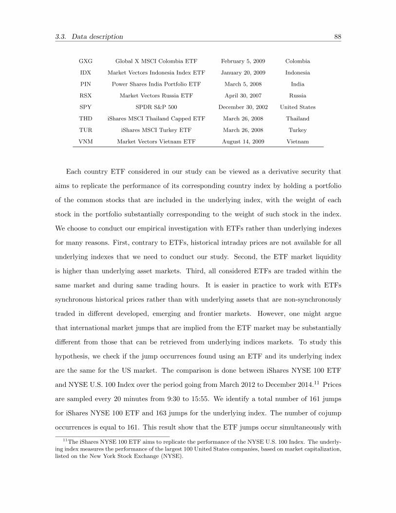
3.3. Data description 88
GXG Global X MSCI Colombia ETF February 5, 2009 Colombia
IDX Market Vectors Indonesia Index ETF January 20, 2009 Indonesia
PIN Power Shares India Portfolio ETF March 5, 2008 India
RSX Market Vectors Russia ETF April 30, 2007 Russia
SPY SPDR S&P 500 December 30, 2002 United States
THD iShares MSCI Thailand Capped ETF March 26, 2008 Thailand
TUR iShares MSCI Turkey ETF March 26, 2008 Turkey
VNM Market Vectors Vietnam ETF August 14, 2009 Vietnam
Each country ETF considered in our study can be viewed as a derivative security that
aims to replicate the performance of its corresponding country index by holding a portfolio
of the common stocks that are included in the underlying index, with the weight of each
stock in the portfolio substantially corresponding to the weight of such stock in the index.
We choose to conduct our empirical investigation with ETFs rather than underlying indexes
for many reasons. First, contrary to ETFs, historical intraday prices are not available for all
underlying indexes that we need to conduct our study. Second, the ETF market liquidity
is higher than underlying asset markets. Third, all considered ETFs are traded within the
same market and during same trading hours. It is easier in practice to work with ETFs
synchronous historical prices rather than with underlying assets that are non-synchronously
traded in different developed, emerging and frontier markets. However, one might argue
that international market jumps that are implied from the ETF market may be substantially
different from those that can be retrieved from underlying indices markets. To study this
hypothesis, we check if the jump occurrences found using an ETF and its underlying index
are the same for the US market. The comparison is done between iShares NYSE 100 ETF
and NYSE U.S. 100 Index over the period going from March 2012 to December 2014.11 Prices
are sampled every 20 minutes from 9:30 to 15:55. We identify a total number of 161 jumps
for iShares NYSE 100 ETF and 163 jumps for the underlying index. The number of cojump
occurrences is equal to 161. This result show that the ETF jumps occur simultaneously with
11The iShares NYSE 100 ETF aims to replicate the performance of the NYSE U.S. 100 Index. The underly-ing index measures the performance of the largest 100 United States companies, based on market capitalization,listed on the New York Stock Exchange (NYSE).

3.4. Empirical Findings 89
its underlying asset. The ETF market can be thus considered as a good proxy to study jumps
of the underlying stock market.
3.4 Empirical Findings
3.4.1 Systematic cojumps
This subsection summarizes the results from applying LM-ABD intraday jump detection
test. Table 3.2 shows the number of total, positive and negative intraday jumps detected over
the period of study. A positive (negative) jump is a jump with positive (negative) return. We
identify 19,599 intraday jumps across all countries in the sample, including the world market
index. The world market index is an equal-weighted portfolio created by giving the same
weight to country ETFs available in the sample for a given day. We identify 681 jumps (59
jumps per year) for the equal-weighted world market index, which corresponds to 1.24% of
the total number of intraday returns over the period of study. We detect 67, 64 and 87 jumps
per year on average for respectively developed, emerging and frontier markets. New Zealand,
Belgium, Frontier markets, Greece and Peru have the largest number of intraday jumps among
all countries studied in our sample. They have more than 80 intraday jumps per year whereas
the average number of jumps is 66 per year. United Kingdom, Thailand, Chile and Australia
have the lowest jump activity with less than 53 jumps per year. Developed countries like the
US, Sweden, France and Germany have similar jump activity to the world market portfolio
with a number of jumps between 58 and 62 per year. The results show the number of negative
jumps is more than 54% of total number of detected jumps across all funds, which is slightly
greater than positive ones. We identify 423 negative systematic jumps for the world market
portfolio, which corresponds to 62% of total systematic jumps. This result indicates that
stock markets tend to be more linked together when prices are decreasing. The gap between
the positive and negative jumps is highest for the world market portfolio, Russia, Indonesia
and Brazil, where the number of negative jumps is respectively 62%, 60%, 60% and 59%. The
proportions of positive jumps are higher than negative ones for Philippines (54% of detected

3.4. Empirical Findings 90
jumps are positive). This table shows jump activity of each country fund. A lower jump
activity implies lower risk (volatility) for investors. Investors should take into account both
the continuous and jump parts of the return before making investment decision.
Table 3.2: Summary statistics of jump occurrences.The percentage of intraday jumps to the number of intraday returns, the percentage of positive jumpsand negative jumps to all jumps are reported in columns 3, 5 and 6, respectively. The total number ofdays available in the sample by fund and the average number of jumps per year are shown in columns2 and 4. Aggregated results are also reported for developed, emerging and frontier markets. Theworld market index is an equal-weighted portfolio created by giving the same weight to country ETFsavailable in the sample. Jumps are detected by LM-ABD procedure. See Appendix 3.A for the jumpmeasure.
Days Intraday jumpsNumber of intraday
jumps per yearPositive jumps Negative jumps
Average - 1.37% 66 46% 54%
Developed markets - 1.39% 67 45% 55%
Emerging markets - 1.33% 64 46% 54%
Frontier markets - 1.83% 87 49% 51%
World Index 2896 681 (1.24%) 59 258 (38%) 423 (62%)
Chile 1518 319 (1.11%) 53 151 (47%) 168 (53%)
New Zealand 817 382 (2.46%) 118 190 (50%) 192 (50%)
Philippines 1052 308 (1.54%) 74 165 (54%) 143 (46%)
Poland 886 207 (1.23%) 59 91 (44%) 116 (56%)
Peru 1372 459 (1.76%) 84 208 (45%) 251 (55%)
Australia 2624 550 (1.1%) 53 246 (45%) 304 (55%)
Canada 2624 592 (1.19%) 57 258 (44%) 334 (56%)
Sweden 2371 556 (1.23%) 59 256 (46%) 300 (54%)
Germany 2624 642 (1.29%) 62 285 (44%) 357 (56%)
Hong Kong 2875 623 (1.14%) 55 275 (44%) 348 (56%)
Italy 2119 556 (1.38%) 66 239 (43%) 317 (57%)
Japan 2894 615 (1.12%) 54 286 (47%) 329 (53%)
Belgium 2371 1074 (2.38%) 114 505 (47%) 569 (53%)
Switzerland 2371 536 (1.19%) 57 243 (45%) 293 (55%)
Malaysia 2371 541 (1.2%) 57 256 (47%) 285 (53%)
Netherlands 2119 655 (1.63%) 78 298 (45%) 357 (55%)
Austria 2624 806 (1.62%) 77 376 (47%) 430 (53%)
Spain 2119 489 (1.21%) 58 219 (45%) 270 (55%)
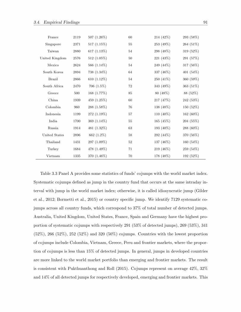
3.4. Empirical Findings 91
France 2119 507 (1.26%) 60 214 (42%) 293 (58%)
Singapore 2371 517 (1.15%) 55 253 (49%) 264 (51%)
Taiwan 2880 617 (1.13%) 54 298 (48%) 319 (52%)
United Kingdom 2576 512 (1.05%) 50 221 (43%) 291 (57%)
Mexico 2624 566 (1.14%) 54 249 (44%) 317 (56%)
South Korea 2894 738 (1.34%) 64 337 (46%) 401 (54%)
Brazil 2866 610 (1.12%) 54 250 (41%) 360 (59%)
South Africa 2470 706 (1.5%) 72 343 (49%) 363 (51%)
Greece 500 168 (1.77%) 85 80 (48%) 88 (52%)
China 1939 459 (1.25%) 60 217 (47%) 242 (53%)
Colombia 960 288 (1.58%) 76 138 (48%) 150 (52%)
Indonesia 1199 272 (1.19%) 57 110 (40%) 162 (60%)
India 1700 369 (1.14%) 55 165 (45%) 204 (55%)
Russia 1914 481 (1.32%) 63 193 (40%) 288 (60%)
United States 2896 662 (1.2%) 58 292 (44%) 370 (56%)
Thailand 1431 297 (1.09%) 52 137 (46%) 160 (54%)
Turkey 1684 478 (1.49%) 71 219 (46%) 259 (54%)
Vietnam 1335 370 (1.46%) 70 178 (48%) 192 (52%)
Table 3.3 Panel A provides some statistics of funds’ cojumps with the world market index.
Systematic cojumps defined as jump in the country fund that occurs at the same intraday in-
terval with jump in the world market index; otherwise, it is called idiosyncratic jump (Gilder
et al., 2012; Bormetti et al., 2015) or country specific jump. We identify 7129 systematic co-
jumps across all country funds, which correspond to 37% of total number of detected jumps.
Australia, United Kingdom, United States, France, Spain and Germany have the highest pro-
portion of systematic cojumps with respectively 291 (53% of detected jumps), 269 (53%), 341
(52%), 266 (52%), 252 (52%) and 320 (50%) cojumps. Countries with the lowest proportion
of cojumps include Colombia, Vietnam, Greece, Peru and frontier markets, where the propor-
tion of cojumps is less than 15% of detected jumps. In general, jumps in developed countries
are more linked to the world market portfolio than emerging and frontier markets. The result
is consistent with Pukthuanthong and Roll (2015). Cojumps represent on average 42%, 32%
and 14% of all detected jumps for respectively developed, emerging and frontier markets. This
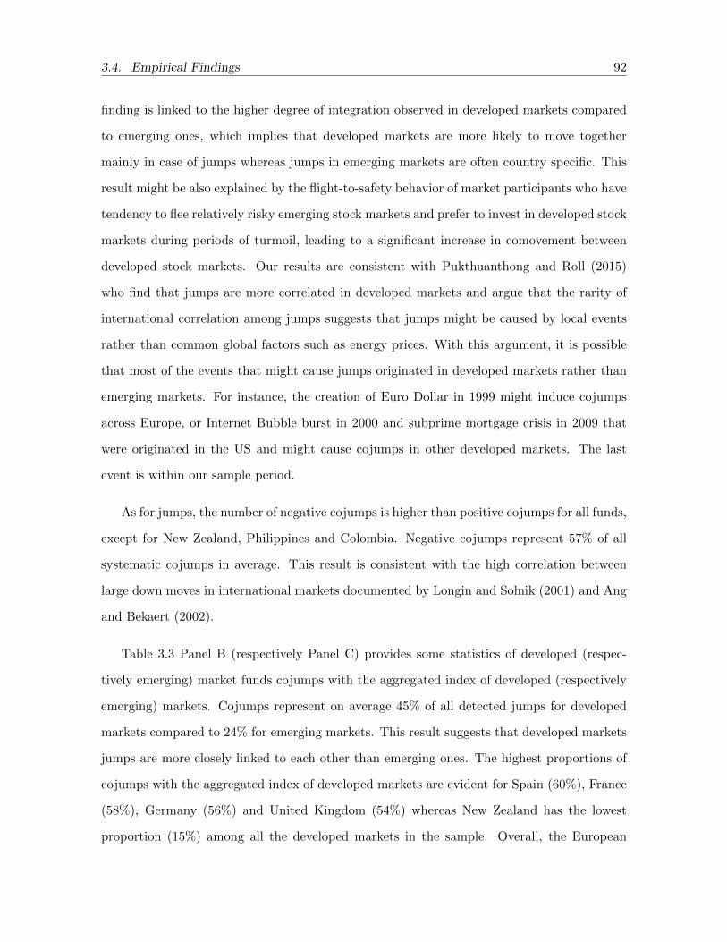
3.4. Empirical Findings 92
finding is linked to the higher degree of integration observed in developed markets compared
to emerging ones, which implies that developed markets are more likely to move together
mainly in case of jumps whereas jumps in emerging markets are often country specific. This
result might be also explained by the flight-to-safety behavior of market participants who have
tendency to flee relatively risky emerging stock markets and prefer to invest in developed stock
markets during periods of turmoil, leading to a significant increase in comovement between
developed stock markets. Our results are consistent with Pukthuanthong and Roll (2015)
who find that jumps are more correlated in developed markets and argue that the rarity of
international correlation among jumps suggests that jumps might be caused by local events
rather than common global factors such as energy prices. With this argument, it is possible
that most of the events that might cause jumps originated in developed markets rather than
emerging markets. For instance, the creation of Euro Dollar in 1999 might induce cojumps
across Europe, or Internet Bubble burst in 2000 and subprime mortgage crisis in 2009 that
were originated in the US and might cause cojumps in other developed markets. The last
event is within our sample period.
As for jumps, the number of negative cojumps is higher than positive cojumps for all funds,
except for New Zealand, Philippines and Colombia. Negative cojumps represent 57% of all
systematic cojumps in average. This result is consistent with the high correlation between
large down moves in international markets documented by Longin and Solnik (2001) and Ang
and Bekaert (2002).
Table 3.3 Panel B (respectively Panel C) provides some statistics of developed (respec-
tively emerging) market funds cojumps with the aggregated index of developed (respectively
emerging) markets. Cojumps represent on average 45% of all detected jumps for developed
markets compared to 24% for emerging markets. This result suggests that developed markets
jumps are more closely linked to each other than emerging ones. The highest proportions of
cojumps with the aggregated index of developed markets are evident for Spain (60%), France
(58%), Germany (56%) and United Kingdom (54%) whereas New Zealand has the lowest
proportion (15%) among all the developed markets in the sample. Overall, the European

3.4. Empirical Findings 93
markets have tendency to cojump more frequently with the aggregate index than other devel-
oped markets in the sample. Thailand, Indonesia and India have the highest proportions of
cojumps with the aggregated index of emerging markets (more than 33% of all detected jumps
for each fund) whereas Colombia, Vietnam, Greece and Peru have the lowest proportions (less
than 10% of all detected jumps for each fund). Globally, Asian stock markets jumps are more
linked to the aggregate index than other emerging markets in the sample. The findings in
this section suggest it is more difficult to diversify portfolio jump risk by investing in Asian
stock market. The results suggest that investors investing in non-Asian emerging markets
may better minimize their exposure to systematic jump risk.
Table 3.3: Summary statistics of systematic cojumps.Panels A, B and C report the number of cojumps, the percentage of cojumps to the total number ofdetected jumps, and the percentage of positive and negative cojumps to all cojumps of all country(respectively developed, emerging and frontier) funds with the world market index (respectively theaggregate index of developed markets, the aggregate index of emerging markets). Panels A, B, and Calso provide the average proportion of cojumps with the word market index for developed, emerging andfrontier markets. The world market index (respectively the developed markets index, emerging marketindex) is an equal-weighted portfolio created by assigning equal weight to all country (respectivelydeveloped, emerging) funds available in the sample. See Appendix 3.A for the cojump measure.
Panel A: Cojumps of all country funds with the world market index
Cojumps Positive cojumps Negative cojumps
Average 37% 43% 57%
Developed markets 42% 43% 57%
Emerging markets 32% 43% 57%
Frontier markets 14% 49% 51%
Chile 66 (21%) 42% 58%
New Zealand 59 (15%) 54% 46%
Philippines 81 (26%) 54% 46%
Poland 95 (46%) 45% 55%
Peru 57 (12%) 46% 54%
Australia 291 (53%) 42% 58%
Canada 236 (40%) 43% 57%
Sweden 256 (46%) 43% 57%
Germany 320 (50%) 41% 59%
Hong Kong 274 (44%) 43% 57%
Italy 235 (42%) 40% 60%

3.4. Empirical Findings 94
Japan 240 (39%) 46% 54%
Belgium 228 (21%) 42% 58%
Switzerland 221 (41%) 43% 57%
Malaysia 202 (37%) 45% 55%
Netherlands 246 (38%) 41% 59%
Austria 221 (27%) 38% 62%
Spain 252 (52%) 42% 58%
France 266 (52%) 36% 64%
Singapore 249 (48%) 47% 53%
Taiwan 260 (42%) 42% 58%
United Kingdom 269(53%) 45% 55%
Mexico 225 (40%) 41% 59%
South Korea 305 (41%) 42% 58%
Brazil 217 (36%) 36% 64%
South Africa 265 (38%) 42% 58%
Greece 19 (11%) 47% 53%
China 200 (44%) 45% 55%
Colombia 28 (10%) 54% 46%
Indonesia 118 (43%) 41% 59%
India 172 (47%) 39% 61%
Russia 217 (45%) 37% 63%
United States 341 (52%) 40% 60%
Thailand 145 (49%) 41% 59%
Turkey 164 (34%) 37% 63%
Vietnam 36 (10%) 47% 53%
Panel B: Cojumps of developed market funds with the aggregate index of developed markets
Cojumps Positive cojumps Negative cojumps
Average 44% 44% 56%
New Zealand 56 (15%) 57% 43%
Australia 290 (53%) 44% 56%
Canada 230 (39%) 45% 55%
Sweden 285 (51%) 46% 54%
Germany 362 (56%) 41% 59%
Hong Kong 257 (41%) 45% 55%

3.4. Empirical Findings 95
Italy 275 (49%) 41% 59%
Japan 238 (39%) 51% 49%
Belgium 261 (24%) 42% 58%
Switzerland 245 (46%) 46% 54%
Netherlands 275 (42%) 42% 58%
Austria 243 (30%) 37% 63%
Spain 293 (60%) 43% 57%
France 294 (58%) 37% 63%
Singapore 235 (45%) 48% 52%
United Kingdom 276 (54%) 46% 54%
South Korea 285 (39%) 46% 54%
United States 321 (48%) 42% 58%
Panel C: Cojumps of emerging market funds with the aggregate index of emerging markets
Cojumps Positive cojumps Negative cojumps
Average 24% 45% 55%
Chile 56 (18%) 46% 54%
Philippines 61 (20%) 51% 49%
Poland 64 (31%) 53% 47%
Peru 40 (9%) 48% 53%
Malaysia 143 (26%) 45% 55%
Taiwan 186 (30%) 45% 55%
Mexico 170 (30%) 45% 55%
Brazil 170 (28%) 38% 62%
South Africa 199 (28%) 41% 59%
Greece 13 (8%) 46% 54%
China 143 (31%) 45% 55%
Colombia 21 (7%) 62% 38%
Indonesia 93 (34%) 40% 60%
India 120 (33%) 38% 63%
Russia 152 (32%) 39% 61%
Thailand 113 (38%) 40% 60%
Turkey 120 (25%) 38% 63%
Vietnam 28 (8%) 46% 54%

3.4. Empirical Findings 96
3.4.2 Diffusive and jump betas
The earlier subsection shows us that country jumps are likely to be linked to each other
especially within developed markets. This correlation between country jumps is an indicator
of a significant systematic jump risk. To assess the exposure of each country fund to market
movements, we apply Todorov and Bollerslev (2010)’s methodology which enable us to de-
compose the systematic market risk (beta) into continuous and jump components. The jump
risk can be decomposed into positive (up), negative (down), small and large betas, which re-
spectively measure the sensitivity of each fund to positive, negative, small and large aggregate
market jumps.
This subsection summarizes the main proprieties of the estimated continuous and discon-
tinuous (up, down, small and large) and overnight betas. We fix the sampling frequency of
intraday returns used in the estimation of these betas at 20 minutes, with returns spanning
from 9:35 am to 4:00 pm for each trading day. We calculate the continuous, discontinuous and
overnight betas on a monthly basis based on the data from the previous 12 months. Table
3.4 Panel A (respectively B, C and D) provides summary statistics of the distributions of the
monthly estimated betas aggregated across all countries (respectively developed, emerging
and frontier markets) and time. We find that the mean and the median of the discontinuous
beta (respectively 1.14 and 1.08) are higher than the continuous one (respectively 1.00 and
0.95) indicating that country funds are more sensitive to the market jumps than to smooth
movements of the market and update faster to unexpected information arrival since jumps
are often associated with macroeconomic news announcements. The standard deviation of
continuous beta (0.28) is lower than discontinuous one (0.35), suggesting that the continuous
beta is less dispersed than the discontinuous beta. We find a similar result for developed,
emerging and frontiers markets. The small jump beta is, on average, greater than large jump
beta indicating that country funds are more sensitive to small frequent market jumps than
large infrequent market jumps. The downside jump beta is, on average, highest among all be-
tas suggesting country funds react to unexpected negative information arrival the most. This

3.4. Empirical Findings 97
result applies to developed, emerging and frontier markets. Overall, the betas are higher for
emerging markets than for developed and frontier markets, implying emerging markets have
higher systematic risks than the other markets. The difference between betas observed in
developed and emerging markets does not necessarily mean that emerging markets are more
linked to aggregate market index than developed ones, but it is simply explained by a higher
level of market volatility in emerging markets compared to developed ones.
Table 3.4: Summary statistics of different betas.Panels A, B, C and D report the mean, median, standard deviation, skewness and kurtosis of monthlyestimated continuous, overnight, discontinuous, discontinuous up, down, large and small betas aggre-gated across all countries (respectively developed, emerging and frontier markets). See Section 3.2 forthe description of each beta measure.
Panel A: All countries
βc βovn βd βd,up βd,down βd,small βd,large
Mean 1.00 1.11 1.14 1.13 1.17 1.12 1.07
Median 0.95 1.07 1.08 1.07 1.09 1.04 1.01
St.deviation 0.28 0.35 0.35 0.35 0.39 0.38 0.43
Skewness 0.74 0.70 1.08 0.94 1.06 1.06 0.56
Kurtosis 3.84 3.92 4.79 6.85 6.36 8.96 6.78
Panel B: developed markets
βc βovn βd βd,up βd,down βd,small βd,large
Mean 0.95 1.08 1.07 1.05 1.09 1.07 1.01
Median 0.92 1.06 1.02 1.02 1.04 1.02 0.97
St.deviation 0.22 0.31 0.31 0.27 0.37 0.32 0.42
Skewness 0.62 0.11 1.17 -0.17 1.13 1.32 0.36
Kurtosis 3.34 3.03 5.86 6.87 8.90 9.32 8.45
Panel C: Emerging markets
βc βovn βd βd,up βd,down βd,small βd,large
Mean 1.08 1.17 1.26 1.25 1.28 1.20 1.17
Median 1.07 1.09 1.19 1.20 1.21 1.16 1.11
St.deviation 0.33 0.40 0.38 0.40 0.40 0.44 0.41
Skewness 0.46 0.92 0.87 1.09 0.99 0.70 0.92
Kurtosis 3.13 3.55 3.85 5.16 4.19 8.25 4.44
Panel D: Frontier markets

3.4. Empirical Findings 98
βc βovn βd βd,up βd,down βd,small βd,large
Mean 0.55 0.60 0.79 0.76 0.88 0.66 0.69
Median 0.53 0.57 0.85 0.82 0.87 0.64 0.73
St.deviation 0.07 0.13 0.14 0.17 0.11 0.17 0.20
Skewness 0.49 0.57 -0.39 -0.52 0.84 0.45 -0.01
Kurtosis 2.09 2.28 2.16 1.79 2.76 2.98 1.77
Figure 3.1 displays the kernel density of the distributions of the monthly estimated con-
tinuous and discontinuous betas aggregated across countries and time. The distributions of
discontinuous betas are right-skewed (a skewness of 1.08 and 0.74 for respectively discontinu-
ous and continuous betas) and fat-tailed (a kurtosis of 3.84 and 4.97, respectively) compared
to the distribution of continuous betas. This result means that large sensitivities of country
funds to market movements are more frequent for intraday market jump returns than for
continuous ones.
Figure 3.1: Beta distributions.The graph displays the kernel density of the distributions of the monthly estimated continuous,overnight, discontinuous, discontinuous up, down, small and large betas aggregated across countriesand time.
3.4.3 Risk factors and portfolio sorts
This subsection examines the cross-sectional relation between estimated betas and return
by forming portfolios ranked on the basis of market betas. At the beginning of each month, we

3.4. Empirical Findings 99
calculate βc, βovn, βd, βd,up, βd,down, βd,small and βd,large using 20 minutes intraday returns
from the previous 12 months. We then sort funds into quintiles (1-5) according to each beta
and form equal-weighted portfolios. The average monthly returns of these sorted portfolios are
computed over the same period used to compute different betas (contemporaneous return).
We also compute the return of these portfolios over the month that follows the estimation
period (post-formation return). Table 3.5 reports the results obtained for the whole period
considered in our study (from July 2003 to December 2014). Panel A shows increasing returns
of portfolios sorted by continuous betas. The difference between the average contemporaneous
returns of the portfolios 1 (high betas) and 5 (low betas) is 0.59% per month. The difference
of average returns is clearly higher between these two portfolios over the month following the
portfolios formation. The post-formation monthly return is equal to 1.35% for the portfolio 1
and 0.32% for the portfolio 5. The Newey-West (1987) heteroskedastic robust t-statistics of
the difference (1.03% per month, 12.35% per annum) is equal to 2.2.12
Panel B shows the results from sorting portfolios based on overnight beta. The average
returns of sorted portfolios do not exhibit a clear relationship with the estimated overnight
beta. Moreover, the difference between the return of the first and last portfolio is not statis-
tically significant at 5% level. This result might be explained by the fact that market news
tend to flow during regular trading hours and not after hours, which increases the variability
of the market during regular hours.
Panels C, D and E show results from sorting portfolios by respectively discontinuous
beta, discontinuous up and down betas. The relation between average returns and market
risk factors is more pronounced for discontinuous down beta than for discontinuous up betas.
First, the returns of portfolios sorted by discontinuous down beta are monotonically increasing
whereas it is not always the case for two others betas. Second, the difference of monthly
returns between the first and last portfolios (0.75% and 0.99% for respectively formation and
post-formation periods) is largest when portfolios are sorted by discontinuous down beta. The
12The Newey-West test is also employed in Ang et al. (2006), Bollerslev et al. (2016) and Alexeev et al.(2017). The Newey-West t-statistic is calculated with 12 lags to adjust for the moving average effects inducedby the use of overlapping estimation period (12 months in our case) for the calculation of monthly betas.
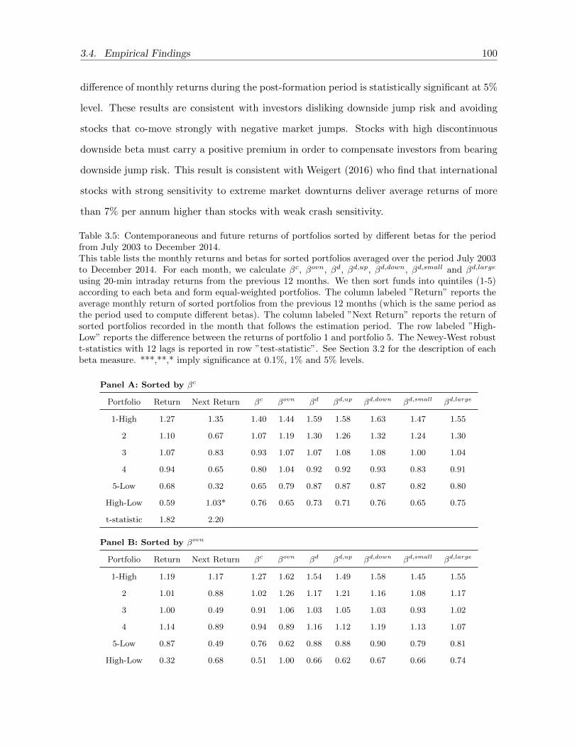
3.4. Empirical Findings 100
difference of monthly returns during the post-formation period is statistically significant at 5%
level. These results are consistent with investors disliking downside jump risk and avoiding
stocks that co-move strongly with negative market jumps. Stocks with high discontinuous
downside beta must carry a positive premium in order to compensate investors from bearing
downside jump risk. This result is consistent with Weigert (2016) who find that international
stocks with strong sensitivity to extreme market downturns deliver average returns of more
than 7% per annum higher than stocks with weak crash sensitivity.
Table 3.5: Contemporaneous and future returns of portfolios sorted by different betas for the periodfrom July 2003 to December 2014.This table lists the monthly returns and betas for sorted portfolios averaged over the period July 2003to December 2014. For each month, we calculate βc, βovn, βd, βd,up, βd,down, βd,small and βd,large
using 20-min intraday returns from the previous 12 months. We then sort funds into quintiles (1-5)according to each beta and form equal-weighted portfolios. The column labeled ”Return” reports theaverage monthly return of sorted portfolios from the previous 12 months (which is the same period asthe period used to compute different betas). The column labeled ”Next Return” reports the return ofsorted portfolios recorded in the month that follows the estimation period. The row labeled ”High-Low” reports the difference between the returns of portfolio 1 and portfolio 5. The Newey-West robustt-statistics with 12 lags is reported in row ”test-statistic”. See Section 3.2 for the description of eachbeta measure. ***,**,* imply significance at 0.1%, 1% and 5% levels.
Panel A: Sorted by βc
Portfolio Return Next Return βc βovn βd βd,up βd,down βd,small βd,large
1-High 1.27 1.35 1.40 1.44 1.59 1.58 1.63 1.47 1.55
2 1.10 0.67 1.07 1.19 1.30 1.26 1.32 1.24 1.30
3 1.07 0.83 0.93 1.07 1.07 1.08 1.08 1.00 1.04
4 0.94 0.65 0.80 1.04 0.92 0.92 0.93 0.83 0.91
5-Low 0.68 0.32 0.65 0.79 0.87 0.87 0.87 0.82 0.80
High-Low 0.59 1.03* 0.76 0.65 0.73 0.71 0.76 0.65 0.75
t-statistic 1.82 2.20
Panel B: Sorted by βovn
Portfolio Return Next Return βc βovn βd βd,up βd,down βd,small βd,large
1-High 1.19 1.17 1.27 1.62 1.54 1.49 1.58 1.45 1.55
2 1.01 0.88 1.02 1.26 1.17 1.21 1.16 1.08 1.17
3 1.00 0.49 0.91 1.06 1.03 1.05 1.03 0.93 1.02
4 1.14 0.89 0.94 0.89 1.16 1.12 1.19 1.13 1.07
5-Low 0.87 0.49 0.76 0.62 0.88 0.88 0.90 0.79 0.81
High-Low 0.32 0.68 0.51 1.00 0.66 0.62 0.67 0.66 0.74

3.4. Empirical Findings 101
t-statistic 0.90 1.52
Panel C: sorted by βd
Portfolio Return Next Return βc βovn βd βd,up βd,down βd,small βd,large
1-High 1.44 1.51 1.31 1.42 1.70 1.59 1.76 1.67 1.57
2 0.88 0.47 1.11 1.28 1.31 1.33 1.31 1.20 1.29
3 1.01 0.94 0.93 1.06 1.07 1.10 1.08 0.97 1.10
4 0.97 0.42 0.81 1.01 0.89 0.92 0.88 0.80 0.87
5-Low 0.70 0.49 0.71 0.78 0.74 0.77 0.73 0.61 0.75
High-Low 0.75 1.02* 0.60 0.64 0.96 0.82 1.03 1.06 0.82
t-statistic 1.88 2.45
Panel D: sorted by βd,up
Portfolio Return Next Return βc βovn βd βd,up βd,down βd,small βd,large
1-High 1.34 1.37 1.34 1.43 1.64 1.64 1.63 1.54 1.54
2 1.00 0.72 1.06 1.24 1.32 1.29 1.34 1.26 1.32
3 1.02 0.81 0.94 1.08 1.10 1.08 1.12 1.06 1.08
4 0.87 0.46 0.82 1.00 0.90 0.91 0.92 0.82 0.88
5-Low 0.82 0.50 0.70 0.77 0.76 0.75 0.80 0.67 0.76
High-Low 0.52 0.87* 0.64 0.66 0.88 0.89 0.83 0.86 0.78
t-statistic 1.35 2.22
Panel E: sorted by βd,down
Portfolio Return Next Return βc βovn βd βd,up βd,down βd,small βd,large
1-High 1.42 1.36 1.29 1.40 1.68 1.54 1.79 1.67 1.56
2 1.07 0.80 1.12 1.26 1.30 1.32 1.31 1.18 1.28
3 0.92 0.65 0.92 1.07 1.07 1.11 1.07 0.97 1.10
4 0.90 0.61 0.82 1.02 0.89 0.93 0.87 0.80 0.87
5-Low 0.68 0.37 0.72 0.81 0.76 0.82 0.71 0.65 0.76
High-Low 0.75 0.99* 0.58 0.59 0.92 0.72 1.07 1.02 0.81
t-statistic 1.92 2.47
Panel F: sorted by βd,small
Portfolio Return Next Return βc βovn βd βd,up βd,down βd,small βd,large
1-High 1.30 1.53 1.26 1.36 1.67 1.55 1.73 1.72 1.48
2 1.08 0.42 1.09 1.25 1.29 1.31 1.30 1.20 1.26
3 0.93 0.74 0.98 1.12 1.08 1.14 1.08 0.96 1.14

3.4. Empirical Findings 102
4 0.90 0.61 0.81 0.99 0.89 0.92 0.88 0.79 0.88
5-Low 0.77 0.48 0.74 0.85 0.77 0.80 0.78 0.58 0.83
High-Low 0.53 1.05** 0.52 0.51 0.90 0.75 0.95 1.14 0.65
t-statistic 1.64 2.86
Panel G: sorted by βd,large
Portfolio Return Next Return βc βovn βd βd,up βd,down βd,small βd,large
1-High 1.12 1.14 1.30 1.47 1.56 1.54 1.59 1.42 1.68
2 1.28 0.90 1.10 1.19 1.35 1.30 1.39 1.30 1.29
3 0.94 1.03 0.95 1.07 1.09 1.11 1.09 1.00 1.05
4 0.96 0.33 0.83 0.99 0.94 0.96 0.94 0.87 0.85
5-Low 0.77 0.54 0.70 0.80 0.80 0.82 0.80 0.75 0.67
High-Low 0.35 0.60 0.60 0.67 0.76 0.72 0.79 0.68 1.01
t-statistic 1.03 1.65
Panels F and G show results from sorting portfolios by respectively discontinuous small
and large betas. The average returns of portfolios sorted by discontinuous small beta are
increasing in function of their exposure to the small market jumps while there is no clear
relationship between average portfolios returns and their exposure to large market jumps. The
difference between the returns of the first and last portfolio sorted by discontinuous large beta
is not statistically significant. Table 3.6 reports the results obtained for the pre-crisis period
from July 2003 to June 2008.13 We notice that the relation between the returns of the sorted
portfolios and different factors of risk (except the overnight beta) is more noticeable during
the pre-crisis period. The t-statistic of the difference between the returns of the first and
last quintile portfolio for contemporaneous return (future return) is 3.56 (3.54), 3.67 (3.11),
3.62 (2.90), 3.59 (2.61) and 3.90 (3.25), 3.18 (1.62) for respectively continuous, discontinuous,
discontinuous up, down, small and large betas. These differences are all significant at 5%
except for the discontinuous large beta.
13We cannot apply the NBER crisis classification due to inadequate number of observations to run Fama-MacBeth regression.

3.4. Empirical Findings 103
Table 3.6: Contemporaneous and future returns of portfolios sorted by different betas during the pre-crisis period (July 2003- June 2008).This table lists the monthly returns and betas for sorted portfolios averaged over the period July2003 to June 2008. For each month, we calculate βc, βovn, βd, βd,up, βd,down, βd,small and βd,large
using 20-min intraday returns from the previous 12 months. We then sort funds into quintiles (1-5)according to each beta and form equal-weighted portfolios. The column labeled ”Return” reports theaverage monthly return of sorted portfolios from the previous 12 months (which is the same period asthe period used to compute different betas). The column labeled ”Next Return” reports the return ofsorted portfolios recorded in the month that follows the estimation period. The row labeled ”High-Low” reports the difference between the returns of portfolio 1 and portfolio 5. The Newey-West robustt-statistics with 12 lags is reported in row ”test-statistic”. See Section 3.2 for the description of eachbeta measure. ***,**,* imply significance at 0.1%, 1% and 5% levels.
Panel A: Sorted by βc
Portfolio Return Next Return βc βovn βd βd,up βd,down βd,small βd,large
1-High 1.62 1.90 1.43 1.48 1.75 1.76 1.78 1.58 1.64
2 1.02 0.80 1.01 1.22 1.43 1.34 1.46 1.39 1.41
3 1.04 0.78 0.89 1.11 1.12 1.14 1.10 1.05 1.04
4 0.53 0.54 0.75 1.09 0.86 0.88 0.85 0.73 0.88
5-Low 0.40 -0.19 0.65 0.79 0.85 0.87 0.84 0.79 0.83
High-Low 1.22*** 2.08*** 0.78 0.69 0.90 0.89 0.94 0.79 0.81
t-statistic 3.56 3.54
Panel B: Sorted by βovn
Portfolio Return Next Return βc βovn βd βd,up βd,down βd,small βd,large
1-High 1.40 1.55 1.28 1.73 1.68 1.62 1.72 1.54 1.68
2 0.89 1.15 0.94 1.30 1.16 1.25 1.11 1.04 1.16
3 0.81 0.01 0.82 1.07 0.99 1.04 0.97 0.88 0.97
4 1.16 1.15 1.00 0.88 1.35 1.30 1.39 1.34 1.19
5-Low 0.67 0.22 0.79 0.55 0.88 0.89 0.90 0.75 0.84
High-Low 0.73 1.33 0.49 1.17 0.80 0.72 0.82 0.80 0.84
t-statistic 1.54 1.56
Panel C: sorted by βd
Portfolio Return Next Return βc βovn βd βd,up βd,down βd,small βd,large
1-High 1.97 2.40 1.32 1.44 1.90 1.73 2.01 1.86 1.71
2 0.79 0.44 1.10 1.38 1.39 1.45 1.38 1.23 1.38
3 0.71 0.81 0.89 1.09 1.08 1.17 1.04 0.92 1.16
4 0.66 -0.13 0.78 1.08 0.84 0.92 0.79 0.73 0.82
5-Low 0.32 0.29 0.68 0.76 0.70 0.74 0.68 0.59 0.70
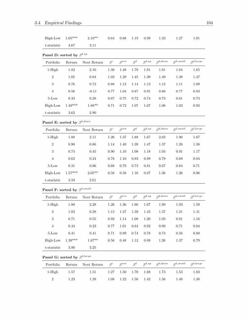
3.4. Empirical Findings 104
High-Low 1.65*** 2.10** 0.64 0.68 1.19 0.99 1.33 1.27 1.01
t-statistic 3.67 3.11
Panel D: sorted by βd,up
Portfolio Return Next Return βc βovn βd βd,up βd,down βd,small βd,large
1-High 1.82 2.16 1.38 1.48 1.79 1.81 1.81 1.64 1.65
2 1.05 0.84 1.02 1.29 1.45 1.39 1.49 1.38 1.47
3 0.76 0.72 0.88 1.12 1.14 1.12 1.12 1.11 1.09
4 0.56 -0.11 0.77 1.04 0.87 0.91 0.86 0.77 0.83
5-Low 0.33 0.28 0.67 0.75 0.72 0.74 0.73 0.61 0.73
High-Low 1.49*** 1.88** 0.71 0.72 1.07 1.07 1.08 1.02 0.92
t-statistic 3.62 2.90
Panel E: sorted by βd,down
Portfolio Return Next Return βc βovn βd βd,up βd,down βd,small βd,large
1-High 1.88 2.11 1.26 1.37 1.88 1.67 2.03 1.90 1.67
2 0.90 0.86 1.14 1.40 1.39 1.47 1.37 1.20 1.38
3 0.74 0.45 0.90 1.10 1.08 1.18 1.03 0.91 1.17
4 0.62 0.24 0.78 1.10 0.83 0.89 0.79 0.69 0.84
5-Low 0.31 0.06 0.68 0.79 0.73 0.81 0.67 0.64 0.71
High-Low 1.57*** 2.05** 0.58 0.58 1.16 0.87 1.36 1.26 0.96
t-statistic 3.59 2.61
Panel F: sorted by βd,small
Portfolio Return Next Return βc βovn βd βd,up βd,down βd,small βd,large
1-High 1.80 2.28 1.26 1.36 1.86 1.67 1.99 1.93 1.59
2 1.03 0.28 1.12 1.37 1.39 1.45 1.37 1.21 1.41
3 0.71 0.55 0.92 1.14 1.08 1.20 1.03 0.91 1.16
4 0.44 0.23 0.77 1.01 0.84 0.92 0.80 0.71 0.84
5-Low 0.41 0.41 0.71 0.89 0.74 0.78 0.73 0.56 0.80
High-Low 1.39*** 1.87** 0.56 0.48 1.12 0.89 1.26 1.37 0.79
t-statistic 3.90 3.25
Panel G: sorted by βd,large
Portfolio Return Next Return βc βovn βd βd,up βd,down βd,small βd,large
1-High 1.57 1.51 1.27 1.50 1.70 1.68 1.73 1.53 1.83
2 1.23 1.28 1.08 1.22 1.50 1.42 1.56 1.48 1.38

3.4. Empirical Findings 105
3 0.71 0.90 0.94 1.12 1.11 1.16 1.09 0.98 1.08
4 0.67 -0.06 0.79 1.06 0.91 0.96 0.88 0.81 0.79
5-Low 0.44 0.42 0.69 0.80 0.77 0.82 0.73 0.69 0.64
High-Low 1.13** 1.09 0.58 0.70 0.94 0.86 1.00 0.84 1.19
t-statistic 3.18 1.62
Table 3.7: Contemporaneous and future returns of portfolios sorted by different betas during the crisisand post-crisis period (July 2008-December 2014).This table lists the monthly returns and betas for sorted portfolios averaged over the period July 2008to December 2014. For each month, we calculate βc, βovn, βd, βd,up, βd,down, βd,small and βd,large
using 20-min intraday returns from the previous 12 months. We then sort funds into quintiles (1-5)according to each beta and form equal-weighted portfolios. The column labeled ”Return” reports theaverage monthly return of sorted portfolios from the previous 12 months (which is the same period asthe period used to compute different betas). The column labeled ”Next Return” reports the return ofsorted portfolios recorded in the month that follows the estimation period. The row labeled ”High-Low” reports the difference between the returns of portfolio 1 and portfolio 5. The Newey-West robustt-statistics with 12 lags is reported in row ”test-statistic”. See Section 3.2 for the description of eachbeta measure. ***,**,* imply significance at 0.1%, 1% and 5% levels.
Panel A: Sorted by βc
Portfolio Return Next Return βc βovn βd βd,up βd,down βd,small βd,large
1-High 0.95 0.85 1.38 1.40 1.45 1.42 1.49 1.38 1.46
2 1.17 0.54 1.12 1.16 1.19 1.18 1.19 1.10 1.20
3 1.10 0.89 0.96 1.04 1.03 1.02 1.05 0.96 1.04
4 1.31 0.75 0.84 0.99 0.98 0.95 1.00 0.92 0.94
5-Low 0.94 0.78 0.64 0.78 0.88 0.87 0.90 0.85 0.77
High-Low 0.02 0.06 0.74 0.62 0.57 0.55 0.59 0.52 0.69
t-statistic 0.04 0.19
Panel B: Sorted by βovn
Portfolio Return Next Return βc βovn βd βd,up βd,down βd,small βd,large
1-High 1.02 0.81 1.26 1.52 1.41 1.38 1.44 1.35 1.42
2 1.12 0.63 1.10 1.22 1.18 1.18 1.20 1.11 1.18
3 1.20 0.94 1.00 1.04 1.06 1.07 1.07 0.97 1.06
4 1.13 0.66 0.89 0.90 0.98 0.97 1.01 0.95 0.96
5-Low 1.08 0.74 0.73 0.67 0.88 0.86 0.91 0.83 0.78
High-Low -0.06 0.08 0.53 0.85 0.53 0.51 0.53 0.52 0.64
t-statistic -0.14 0.20
Panel C: sorted by βd

3.4. Empirical Findings 106
Portfolio Return Next Return βc βovn βd βd,up βd,down βd,small βd,large
1-High 0.96 0.69 1.30 1.41 1.52 1.47 1.54 1.50 1.45
2 0.97 0.49 1.11 1.18 1.23 1.22 1.24 1.18 1.19
3 1.29 1.07 0.97 1.04 1.06 1.04 1.11 1.02 1.04
4 1.24 0.93 0.84 0.95 0.93 0.92 0.96 0.87 0.91
5-Low 1.04 0.67 0.74 0.80 0.77 0.79 0.78 0.63 0.80
High-Low -0.07 0.02 0.56 0.60 0.75 0.68 0.75 0.87 0.65
t-statistic -0.21 0.08
Panel D: sorted by βd,up
Portfolio Return Next Return βc βovn βd βd,up βd,down βd,small βd,large
1-High 0.90 0.64 1.30 1.39 1.50 1.49 1.47 1.45 1.44
2 0.95 0.62 1.11 1.20 1.21 1.21 1.21 1.14 1.19
3 1.26 0.90 0.99 1.04 1.07 1.05 1.11 1.01 1.07
4 1.14 0.99 0.85 0.95 0.94 0.92 0.97 0.86 0.93
5-Low 1.26 0.71 0.73 0.79 0.80 0.77 0.87 0.73 0.78
High-Low -0.36 -0.07 0.58 0.60 0.70 0.73 0.60 0.72 0.66
t-statistic -1.18 -0.35
Panel E: sorted by βd,down
Portfolio Return Next Return βc βovn βd βd,up βd,down βd,small βd,large
1-High 1.00 0.66 1.32 1.42 1.49 1.41 1.56 1.45 1.46
2 1.23 0.74 1.09 1.14 1.21 1.19 1.26 1.16 1.19
3 1.08 0.84 0.94 1.04 1.06 1.05 1.10 1.02 1.04
4 1.15 0.95 0.87 0.95 0.96 0.97 0.95 0.90 0.91
5-Low 1.01 0.65 0.74 0.82 0.79 0.83 0.76 0.66 0.80
High-Low 0.00 0.01 0.58 0.60 0.70 0.58 0.81 0.80 0.67
t-statistic -0.01 0.02
Panel F: sorted by βd,small
Portfolio Return Next Return βc βovn βd βd,up βd,down βd,small βd,large
1-High 0.85 0.83 1.25 1.36 1.49 1.44 1.49 1.54 1.38
2 1.12 0.56 1.07 1.14 1.20 1.17 1.23 1.19 1.13
3 1.14 0.91 1.04 1.10 1.08 1.08 1.12 1.01 1.12
4 1.32 0.95 0.84 0.96 0.93 0.93 0.97 0.85 0.93
5-Low 1.10 0.55 0.77 0.82 0.80 0.82 0.82 0.60 0.86

3.4. Empirical Findings 107
High-Low -0.26 0.28 0.48 0.53 0.69 0.62 0.67 0.94 0.52
t-statistic -1.31 1.00
Panel G: sorted by βd,large
Portfolio Return Next Return βc βovn βd βd,up βd,down βd,small βd,large
1-High 0.71 0.80 1.32 1.44 1.43 1.41 1.46 1.33 1.55
2 1.32 0.55 1.12 1.17 1.20 1.18 1.24 1.14 1.21
3 1.16 1.15 0.95 1.03 1.07 1.06 1.09 1.02 1.03
4 1.23 0.70 0.86 0.93 0.97 0.97 0.98 0.93 0.90
5-Low 1.07 0.64 0.71 0.80 0.84 0.83 0.86 0.80 0.70
High-Low -0.36 0.16 0.61 0.64 0.9 0.58 0.59 0.53 0.84
t-statistic -1.01 0.65
Table 3.7 reports the results obtained for the crisis and post-crisis periods from July 2008
to December 2014. We notice that the difference between the contemporaneous returns of
the first and last quintile portfolio is negative for overnight, discontinuous, discontinuous up,
small and large betas. The return difference is highest in absolute value for discontinuous
up and large betas (-0.36). However, contemporaneous and future returns differences are not
significant at 5% for all betas. During the crisis and pre-crisis period, we observe an inversion
of the patterns of realized returns for portfolios sorted on jump betas (expect for discontinuous
downside beta). This result is consistent with an increasing investor appetite for equities that
positively co-move with large and positive market jumps during periods of market turmoil.
These equities will help investors to better hedge against large movements of market and thus
would require lower expected returns.
3.4.4 Fama-MacBeth regressions
It is well established in the financial literature that only systematic risk is rewarded by
premium. In our four-factor model, the systematic risk is decomposed into four components:
the risk of exposure to smooth or continuous fluctuations of the market, the risk of exposure to
overnight movements of the market price, the risk of exposure to positive (small) discontinuous

3.4. Empirical Findings 108
movements of the market and the risk of exposure to negative (large) discontinuous movements
of the market.
After estimating the sensitivity of each country fund towards the different risk factors,
we follow Fama and MacBeth (1973)’s approach and run the following set of cross-sectional
regressions for each month in the sample:
ri,t = αi,t + βci,tγct + βdi,tγ
dt + βovni,t γ
ovnt + εi,t (I)
ri,t = αi,t + βci,tγct + βd,upi,t γd,upt + βd,downi,t γd,downt + βovni,t γ
ovnt + εi,t (II)
ri,t = αi,t + βci,tγct + βd,smalli,t γd,smallt + βd,largei,t γd,larget + βovni,t γ
ovnt + εi,t (III)
where ri,t is the average return of fund i on month t calculated as an arithmetic average
of previous 12 monthly returns. Different betas are computed on a monthly basis over the
previous 12 months, which is the same period used to calculate the return. γct , γdt , γovnt , γd,upt ,
γd,downt , γd,smallt and γd,larget are the coefficients of the three regressions on month t. Based on
the monthly estimates of these coefficients, we estimate the risk premia associated with the
different risk factors by taking the mean of the estimates:
γk =1
Nm
Nm∑t=1
γkt , k = (c; d; ovn; d, up; d, down; d, small; d, large)
where Nm is the number of months in the sample (126 months in our sample).
Once risk premia are calculated, it is possible to deduce the investor’s risk aversion coef-
ficient based on the expected utility theory. To this end, we assume that the representative
investor has a power utility function U with a constant relative risk aversion coefficient η and
an initial wealth W0 equal to 1. The market risk premium γ can be seen as the price that the
investor is ready to pay to get rid of the zero-mean market risk, r0 = r0 − E(r0):
U(W0 − γ) = E(U(W0 + r0))

3.4. Empirical Findings 109
Using Taylor series expansions around γ = 0 and r0 = 0, the risk aversion coefficient can
be approximated as follows:14
η =−W0U
′′(W0)
U ′(W0)≈ 2γ
σ20
where σ20 = E(r2
0) is the variance of the market return. It should be noted that the previous
formula of risk aversion coefficient only holds for a positive risk premium.
Table 3.8 Panels A, B and C report the results of the cross-sectional regressions for re-
spectively the whole period (from July 2003 to December 2014), the pre-crisis period (from
July 2003 to June 2008) and the crisis and post-crisis period (from July 2008 to December
2014). The risk premia estimated using all data available from July 2003 to December 2014
are not significant at 5% level, except for the continuous beta in regressions I and III. The
reward for continuous risk becomes insignificant when the discontinuous risk is decomposed
into downside and upside components (regression II).
If we only restrict our analysis to the pre-crisis period, we find that both continuous
and discontinuous betas’ premia (respectively 1.4% and 0.7% per month) are statistically
significant at 0.1% and 5% level (regression I), respectively. In regression II, only the premium
awarded to the downside jump risk (0.79%) is significant at 5% level. In regression III, only
the continuous beta premium (1.8%) is significant at 1% level. By averaging continuous and
discontinuous risk premia found across three regressions during the pre-crisis period, we get
an average market risk premium of 1.56% per month and a risk aversion coefficient of 5.5.
The risk premia during the crisis and post-crisis period are not significant except for the
upside and large discontinuous betas in regression II and III. Interestingly, these two betas
are associated with a negative premium (-0.9% for upside jump risk and -0.48% for large
jump risk). This finding is consistent with common economic theory that investors may
seek to hedge themselves against large movements of market, mainly during financial crisis
period. In this case, equities that positively co-move with large and positive market jumps are
14We use a first-order approximation for the first term U(W0 − γ) = U(W0)− γU ′(W0) and a second-order
approximation for the second term E(U(W0 + r0)) = U(W0) +σ202U ′′(W0).

3.4. Empirical Findings 110
particularly attractive for investors and thus would require lower expected returns.15 Overall,
the reward for bearing continuous and downside discontinuous risks are positively priced in
the cross-section of expected stock returns during the pre-crisis period whereas the upside
and large jump risks are negatively priced during the crisis and post-crisis period.
Table 3.8: Fama-MacBeth regressions.This table shows the results of Fama-MacBeth regressions of 12-month average returns on risk char-acteristics. The Newey-West t-statistics of the estimated parameters are given between parentheses.Panels A, B, and C report the results for respectively the whole period (July 2003-December 2014),the pre-crisis period (July 2003-June 2008) and the crisis and post-crisis period (July 2008-December2014). See Section 3.2 for the description of each beta measure. ***,**,* imply significance at 0.1%,1% and 5% levels.
Panel A: Whole period (July 2003-December 2014)
Regression βc βovn βd βd,up βd,down βd,small βd,large
I 0.0093** -0.0013 0.0006
(2.67) (-0.38) (0.10)
II 0.0065 -0.0008 -0.0027 0.0060
(1.34) (-0.24) (-0.71) (1.15)
III 0.0119** 0.0002 -0.0019 -0.0006
(2.88) (0.07) (-0.62) (-0.26)
Panel B: Pre-Crisis period (July 2003-June 2008)
Regression βc βovn βd βd,up βd,down βd,small βd,large
I 0.0144*** -0.0038 0.0070*
(4.63) (-0.69) (2.09)
II 0.0092 -0.0025 0.0042 0.0079*
(1.19) (-0.46) (0.83) (1.99)
III 0.0181** -0.0018 -0.0009 0.004
(3.08) (-0.36) (-0.24) (1.65)
Panel C: Crisis and Post-Crisis period (July 2008-December 2014)
Regression βc βovn βd βd,up βd,down βd,small βd,large
I 0.0047 0.0009 -0.0052
(0.92) (0.19) (-0.61)
II 0.0042 0.0007 -0.009** 0.0042
(0.70) (0.16) (-3.06) (0.46)
15Cremers et al. (2015) find that both volatility and jump risks are negatively priced in the cross-section ofreturns but they do not decompose the jump risk into upside/downside or small/large components.

3.4. Empirical Findings 111
III 0.0062 0.0021 -0.0029 -0.0048**
(1.36) (0.42) (-0.60) (-2.28)
3.4.5 Currency jump risk premium
This subsection considers another source of jumps and cojumps between international
stock markets, the currency jump risk. The exposure of international portfolios to foreign
exchange market movements can be explained by at least two factors. First, international
portfolios are composed of domestic and foreign assets. The foreign assets that are expressed
in domestic currency are exposed to two types of variability: the stock market variability and
foreign exchange market variability. The return of international portfolio is thus affected by
both stock and exchange markets movements. Second, the exposure of international portfolios
to currency risk may come from the correlation between stock and foreign exchange markets.
To assess how country funds react to foreign exchange markets, we consider the number
of cojumps of each fund with EUR/USD exchange rate. We choose EUR and USD because
they are the two most traded currencies in the world. Also, all considered funds are expressed
in USD. As shown in Table 3.9, the cojumps between EUR/USD and the world market
portfolio is 22% of all detected jumps. Spain, Switzerland, Germany, and France have the
highest proportion of cojumps with respectively 28%, 27%, 26% and 24% of all detected jumps.
Countries with the lowest proportion of cojumps with EUR/USD exchange rate include Chile,
Peru, Greece, Colombia, Vietnam and frontier markets, where the proportion of cojumps is
less than 10% of detected jumps. In general, the proportion of cojumps between European
stock markets and EUR/USD exchange rate is higher than other developed and emerging
markets.

3.4. Empirical Findings 112
Table 3.9: Cojumps between stock markets and EUR/USD exchange rate.The table reports the percentage of cojumps to the total number of detected jumps of all country fundswith the EUR/USD exchange rate. The percentage of cojumps with the world market index is alsoprovided. The world market index is an equal-weighted portfolio created by assigning equal weightto all country funds available in the sample. See Appendix 3.A for the cojump measure. Jumps andcojumps are detected for the period going from July 2003 to December 2014.
Cojumps
World market index 22%
Frontier markets 8%
Chile 9%
New Zealand 11%
Philippines 11%
Poland 16%
Peru 7%
Australia 23%
Canada 16%
Sweden 23%
Germany 26%
Hong Kong 14%
Italy 20%
Japan 16%
Belgium 17%
Switzerland 27%
Malaysia 13%
Netherlands 19%
Austria 15%
Spain 28%
France 24%
Singapore 18%
Taiwan 14%
United Kingdom 23%
Mexico 17%
South Korea 13%
Brazil 14%
South Africa 15%
Greece 5%

3.4. Empirical Findings 113
China 15%
Colombia 6%
Indonesia 18%
India 19%
Russia 17%
United States 15%
Thailand 18%
Turkey 16%
Vietnam 6%
To evaluate the price of the jump currency risk in the cross-section of stock returns, we
consider the three cross-sectional regressions introduced in Section 3.4.4 with an additional
factor of risk representing the sensitivity of an asset i to EUR/USD exchange rate jump
movements, βd,currencyi,t .
ri,t = αi,t + βci,tγct + βdi,tγ
dt + βd,currencyi,t γd,currencyt + βovni,t γ
ovnt + εi,t (I)
ri,t = αi,t + βci,tγct + βd,upi,t γd,upt + βd,downi,t γd,downt + βd,currencyi,t γd,currencyt + βovni,t γ
ovnt + εi,t (II)
ri,t = αi,t + βci,tγct + βd,smalli,t γd,smallt + βd,largei,t γd,larget + βd,currencyi,t γd,currencyt + βovni,t γ
ovnt + εi,t (III)
where γd,currencyt is the risk premium associated with the EUR/USD jump risk. βd,currencyi,t is
calculated similarly to the discontinuous beta (formula given in Section 3.2). We only replace
the aggregate market index returns by EUR/USD exchange rate returns.
Table 3.10 Panels A, B and C report the results of the cross-sectional regressions for
respectively the whole period (from July 2003 to December 2014), the pre-crisis period (from
July 2003 to June 2008) and the crisis and post-crisis period (from July 2008 to December
2014). We find that the currency jump risk premium is not significant for the three considered
periods. Previous results on continuous and discontinuous equity jump risk premia remain
intact. The reward for bearing continuous and downside discontinuous risks are positively
priced in the cross-section of expected stock returns during the pre-crisis period whereas the
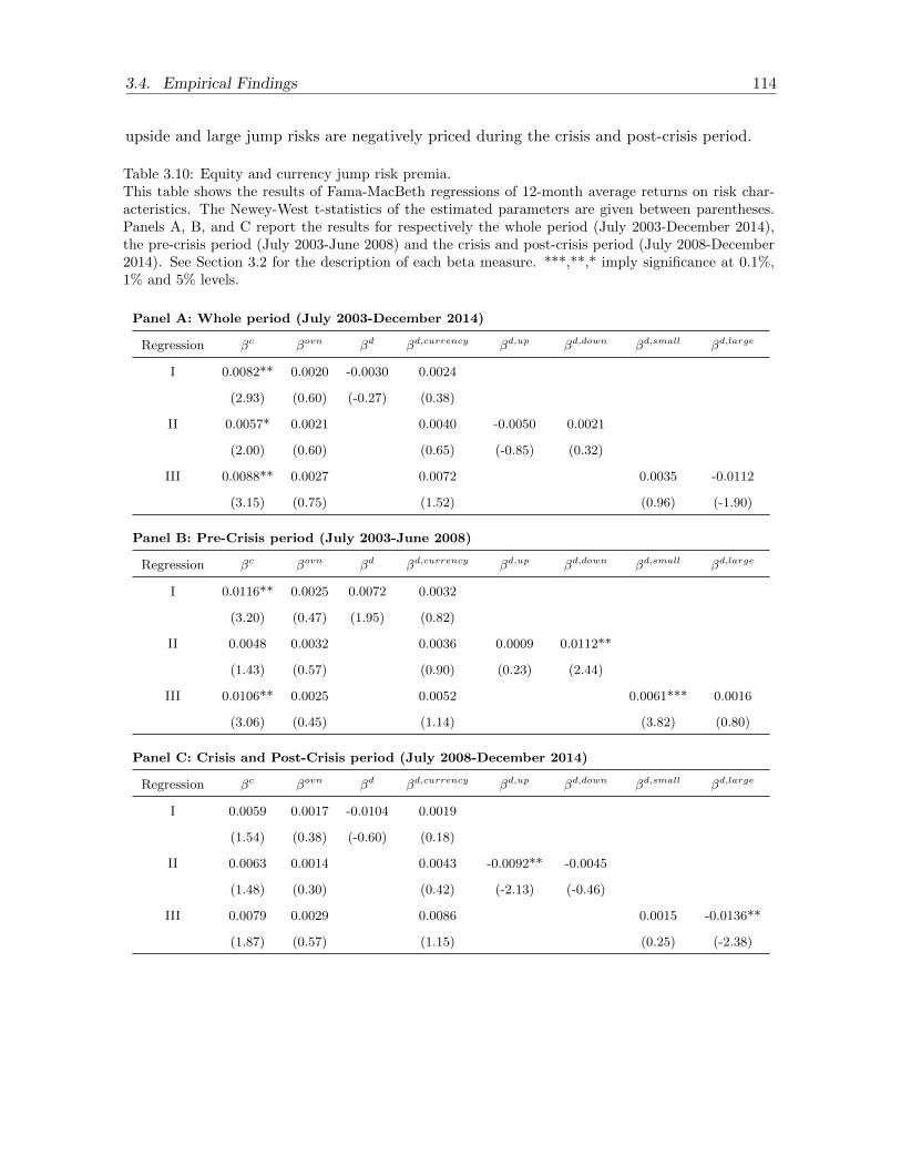
3.4. Empirical Findings 114
upside and large jump risks are negatively priced during the crisis and post-crisis period.
Table 3.10: Equity and currency jump risk premia.This table shows the results of Fama-MacBeth regressions of 12-month average returns on risk char-acteristics. The Newey-West t-statistics of the estimated parameters are given between parentheses.Panels A, B, and C report the results for respectively the whole period (July 2003-December 2014),the pre-crisis period (July 2003-June 2008) and the crisis and post-crisis period (July 2008-December2014). See Section 3.2 for the description of each beta measure. ***,**,* imply significance at 0.1%,1% and 5% levels.
Panel A: Whole period (July 2003-December 2014)
Regression βc βovn βd βd,currency βd,up βd,down βd,small βd,large
I 0.0082** 0.0020 -0.0030 0.0024
(2.93) (0.60) (-0.27) (0.38)
II 0.0057* 0.0021 0.0040 -0.0050 0.0021
(2.00) (0.60) (0.65) (-0.85) (0.32)
III 0.0088** 0.0027 0.0072 0.0035 -0.0112
(3.15) (0.75) (1.52) (0.96) (-1.90)
Panel B: Pre-Crisis period (July 2003-June 2008)
Regression βc βovn βd βd,currency βd,up βd,down βd,small βd,large
I 0.0116** 0.0025 0.0072 0.0032
(3.20) (0.47) (1.95) (0.82)
II 0.0048 0.0032 0.0036 0.0009 0.0112**
(1.43) (0.57) (0.90) (0.23) (2.44)
III 0.0106** 0.0025 0.0052 0.0061*** 0.0016
(3.06) (0.45) (1.14) (3.82) (0.80)
Panel C: Crisis and Post-Crisis period (July 2008-December 2014)
Regression βc βovn βd βd,currency βd,up βd,down βd,small βd,large
I 0.0059 0.0017 -0.0104 0.0019
(1.54) (0.38) (-0.60) (0.18)
II 0.0063 0.0014 0.0043 -0.0092** -0.0045
(1.48) (0.30) (0.42) (-2.13) (-0.46)
III 0.0079 0.0029 0.0086 0.0015 -0.0136**
(1.87) (0.57) (1.15) (0.25) (-2.38)
3.4. Empirical Findings 115
3.4.6 Equity risk premia and the leverage effect
The earlier subsection shows that investors require positive premia for bearing respectively
the continuous and downside jump market risks during the pre-crisis period. In this subsec-
tion, we examine the potential channels through which the diffusive and discontinuous shocks
of the asset price process affect the equity risk premium. We hypothesize that investors are
not only compensated for their exposure to continuous and discontinuous price fluctuations,
but also for the negative relationship between the return and volatility movements, commonly
called the ”leverage effect” in the finance literature. Indeed, the burgeoning literature includ-
ing our paper has shown evidence of asymmetry in the relationship between equity market
returns and volatility and different explanations have been proposed.
The first leading explanation for the return-volatility asymmetry is based on time-varying
risk premia or ”volatility feedback effect” as studied by French et al. (1987) and Campbell
and Hentschel (1992). The authors find a strong negative relationship between realized excess
holding period returns and the unpredictable component of volatility, which they interpret
as indirect evidence of a positive ex ante relationship between return and risk. They argue
if volatility is priced, an increase in unexpected volatility would increase the future required
rate of return and decrease current stock prices.
Black (1976) and Christie (1982) propose another explanation based on leverage. They
suggest that negative returns should raise the firm leverage, leading to higher future volatility
whereas positive returns should reduce the firm leverage resulting in a decrease in subsequent
volatility. Figlewski and Wang (2000) extend this argument and show the magnitude of
the effect of a decline in current price on future volatility is too large to be explained only
by changes in financial leverage. That is, the leverage-based explanation states that a fall in
stock price should increase subsequent volatility. In theory, a price rise of the same magnitude
should induce volatility reduction in the same amount; however, Figlewski and Wang (2000)
show that the impact is more pronounced during the down market than during the up time.
In what follows, we examine the role of the return-volatility asymmetry in determining the

3.4. Empirical Findings 116
equity risk premium. We assume that the log-price process of the aggregate market index p0,t
follows a stochastic volatility model with cojumps between the price and volatility processes:
dp0,t = αtdt+ σtdW1t + Jrt dQ
rt + Jr,cot dQr,vt
d log(σ2t ) = αvt dt+ σvt dW
2t + Jvt dQ
vt + Jv,cot dQr,vt
where αt and σt are respectively the drift and the volatility of the diffusive component of the
price process. αvt and σvt are respectively the drift and the volatility of the diffusive part of
the volatility process. The jump component of the price process is composed of independent
jumps with size Jrt and a Poisson process Qrt with intensity λrt , and common jumps with the
volatility process characterized with a size Jr,cot and a Poisson process Qr,vt with intensity
λr,vt . Similarly, the volatility process is characterized by independent jumps with size Jvt
and a Poisson process Qvt with intensity λvt , and cojumps with the price process with size
Jv,cot and a Poisson process Qr,vt with intensity λr,vt . The Brownian motions W 1t and W 2
t are
negatively correlated with a correlation coefficient ρt. The negative covariation between asset
returns and volatility changes stems from the negative correlation of diffusive shocks as well
as simultaneous and anti-correlated jumps of both processes.
We also assume the existence of a stochastic discount factor Mt defined as follows:16
d log(Mt) = δtdt+ φdp0,t + ψd log(σ2t )
where δt is a function controlling the time preferences. φ and ψ are parameters controlling the
aversion to respectively the price risk and the variance risk. The stochastic discount factor is
decreasing in prices (φ < 0) and increasing in variance (ψ > 0).
As shown in Bandi and Reno (2016), the expression of the return risk premium γ is given
16This pricing kernel has been also employed in Bandi and Reno (2016).

3.4. Empirical Findings 117
by:17
γ = αt +σ2t
2− rf = −φσ2
t − ψρtσtσvt − λrtE[eφJrt (eJ
rt − 1)]− λr,vt E[eφJ
r,cot +ψJv,cot (eJ
r,cot − 1)]
where rf is the risk-free rate.
The expression of the return risk premium is composed of four terms. The first term is the
price of the diffusive return risk. The second term is the reward required to compensate the
”leverage effect” induced by the negative correlation between continuous return and volatility
changes. The third term represents the reward for bearing the return jump risk whereas
the fourth term corresponds to the price of the discontinuous ”leverage effect” induced by
anti-correlated return and volatility cojumps.
We examine the validity of our hypothesis by estimating both the continuous and discon-
tinuous components of the covariation between the asset returns and the volatility. We follow
Ait-Sahalia et al. (2017) who provide consistent estimators for continuous (henceforth CLE)
and discontinuous (henceforth DLE) leverage effects using high frequency data:
CLE =
mT−lm∑τ=lm+1
∆p0,τ1|∆p0,τ |≤θ0,τ(σ2τ+ − σ2
τ−)
DLE =
mT−lm∑τ=lm+1
∆p0,τ1|∆p0,τ |>θ0,τ(σ2τ+ − σ2
τ−)
where σ2τ+ and σ2
τ− are estimates of the spot variance just before and after time τm :
σ2τ+ =
m
lm
τ+lm∑τ ′=τ+1
(∆p0,τ ′)21|∆p0,τ ′ |≤θ0,τ ′
σ2τ− =
m
lm
τ−1∑τ ′=τ−lm
(∆p0,τ ′)21|∆p0,τ ′ |≤θ0,τ ′
17This expression can be found by applying Ito’s lemma to the martingale processes Mterf t and Mte
pt .

3.4. Empirical Findings 118
where lmm defines the length of the local averaging widows for the estimation of the pre-
and post-variances. We also decompose the discontinuous leverage effect into upside and
downside components by applying the DLE’s formula to respectively positive and negative
market returns.
Table 3.11 reports the results of the estimation of the continuous, discontinuous, discon-
tinuous up and discontinuous down leverage effects of the world market index for respectively
the whole sample period, the pre-crisis period and the crisis and post-crisis period. The con-
tinuous and downside discontinuous covariations between the return and the volatility changes
are significantly negative during the pre-crisis period with a value of -0.44 and -0.10, respec-
tively. The negative relationship between continuous parts of the return and the volatility
processes means that smooth movements of market prices are associated with smooth oppo-
site variations of the volatility. Similarly, the negative downside discontinuous covariation
indicates that negative jumps of the aggregate market index are often associated with con-
temporaneous positive jumps of market volatility. The contemporaneous negative covariation
between return and volatility jumps can be considered as evidence in favor of an almost in-
stantaneous discontinuous volatility feedback effect, meaning that an upward volatility jump
is immediately followed by a downward return jump. It also suggests that, like the downside
return jump risk, the upside volatility jump risk should also be priced in the cross-section of
returns during the pre-crisis period. This finding is consistent with Bollerslev et al. (2006)
who also provide evidence of a strong contemporaneous negative correlation between the high
frequency returns and the volatility. However, those authors do not decompose the return
into continuous and discontinuous components.
Moreover, the results show a significant asymmetry between the upside and downside
components of the discontinuous leverage effects during the pre-crisis period, such that the
covariation between downside return jumps and upside volatility jumps (downside DLE) is
significantly negative (-0.10) whereas the covariation between upside return jumps and down-
side volatility jumps (upside DLE) is weak, and even positive (0.07). These findings contradict
the leverage-based explanation of the negative return-volatility relationship that suggests that
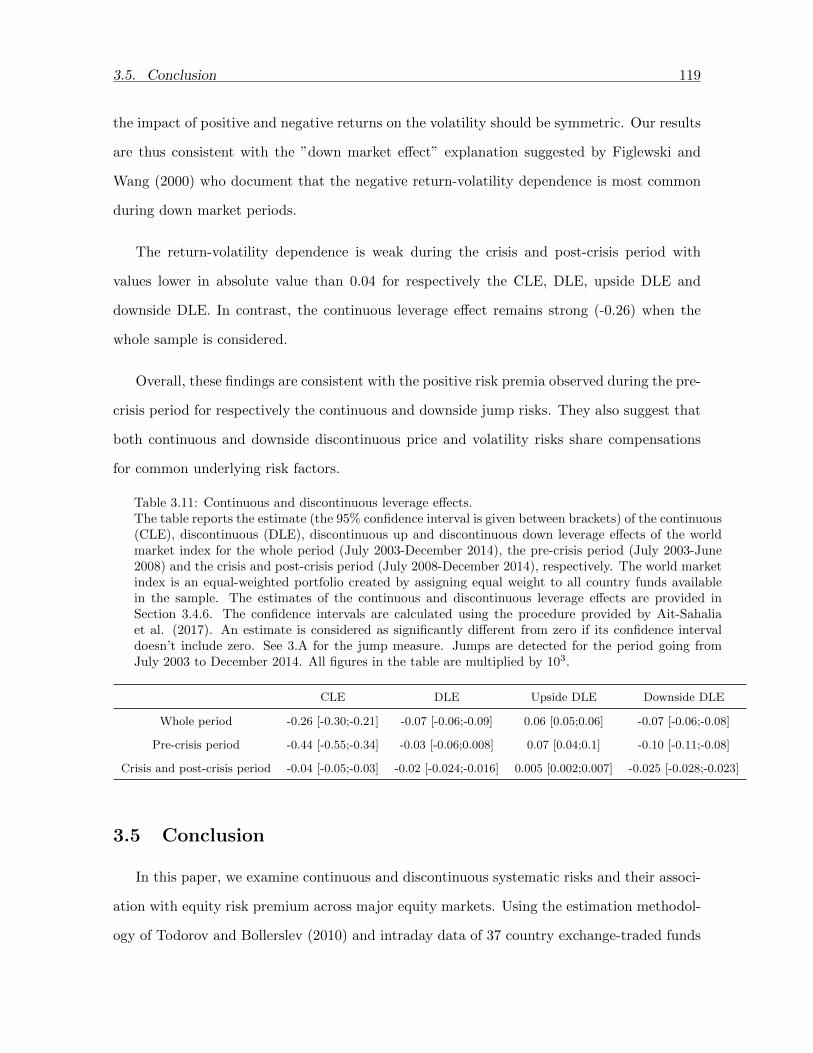
3.5. Conclusion 119
the impact of positive and negative returns on the volatility should be symmetric. Our results
are thus consistent with the ”down market effect” explanation suggested by Figlewski and
Wang (2000) who document that the negative return-volatility dependence is most common
during down market periods.
The return-volatility dependence is weak during the crisis and post-crisis period with
values lower in absolute value than 0.04 for respectively the CLE, DLE, upside DLE and
downside DLE. In contrast, the continuous leverage effect remains strong (-0.26) when the
whole sample is considered.
Overall, these findings are consistent with the positive risk premia observed during the pre-
crisis period for respectively the continuous and downside jump risks. They also suggest that
both continuous and downside discontinuous price and volatility risks share compensations
for common underlying risk factors.
Table 3.11: Continuous and discontinuous leverage effects.The table reports the estimate (the 95% confidence interval is given between brackets) of the continuous(CLE), discontinuous (DLE), discontinuous up and discontinuous down leverage effects of the worldmarket index for the whole period (July 2003-December 2014), the pre-crisis period (July 2003-June2008) and the crisis and post-crisis period (July 2008-December 2014), respectively. The world marketindex is an equal-weighted portfolio created by assigning equal weight to all country funds availablein the sample. The estimates of the continuous and discontinuous leverage effects are provided inSection 3.4.6. The confidence intervals are calculated using the procedure provided by Ait-Sahaliaet al. (2017). An estimate is considered as significantly different from zero if its confidence intervaldoesn’t include zero. See 3.A for the jump measure. Jumps are detected for the period going fromJuly 2003 to December 2014. All figures in the table are multiplied by 103.
CLE DLE Upside DLE Downside DLE
Whole period -0.26 [-0.30;-0.21] -0.07 [-0.06;-0.09] 0.06 [0.05;0.06] -0.07 [-0.06;-0.08]
Pre-crisis period -0.44 [-0.55;-0.34] -0.03 [-0.06;0.008] 0.07 [0.04;0.1] -0.10 [-0.11;-0.08]
Crisis and post-crisis period -0.04 [-0.05;-0.03] -0.02 [-0.024;-0.016] 0.005 [0.002;0.007] -0.025 [-0.028;-0.023]
3.5 Conclusion
In this paper, we examine continuous and discontinuous systematic risks and their associ-
ation with equity risk premium across major equity markets. Using the estimation methodol-
ogy of Todorov and Bollerslev (2010) and intraday data of 37 country exchange-traded funds

3.5. Conclusion 120
covering developed, emerging and frontier markets from July 2003 to December 2014, we esti-
mate the exposure of each country fund returns towards six separate market risks: continuous,
overnight, discontinuous up, down, small and large market risks. We find that cojumps are
more frequent in developed markets than emerging markets, which is inline with the nature
of high market integration in developed markets. We also find that emerging stock markets,
particularly non-Asian emerging markets, still offer a good opportunity for investors to reduce
their exposure to market risk for the various systematic risks considered in our study.
The results of portfolio sorting approach and the cross-sectional Fama and MacBeth (1973)
regressions show that continuous and downside discontinuous risks are positively priced in the
cross-section of expected stock returns during the pre-crisis period whereas the upside and
large jump risks are negatively priced during the crisis and post-crisis periods, suggesting that
investors prefer stocks that help them hedge against large movements of the market during
the crisis period. Finally, we provide evidence on the strong negative relationship between
market price movements and market volatility changes during the pre-crisis period, which
is consistent with the positive continuous and downside jump premia observed during the
pre-crisis period.
This work opens interesting perspectives for future research. It would be of interest to
develop new methods for computing the portfolio value-at-risk (VAR) based on the market risk
decomposition provided in the paper. Studying the underlying mechanisms of the continuous
and discontinuous price and volatility covariations should also be of interest.

References
Ait-Sahalia, Y., Cacho-Diaz, J., and Laeven, R., 2015. Modeling financial contagion using
mutually exciting jump processes. Journal of Financial Economics 117, 585-606.
Ait-Sahalia, Y., Fan, J. , Laeven, R.J. A., Wang, C.D, and Yang, X., 2017. Estimation of
the Continuous and Discontinuous Leverage Effects. Journal of the American Statistical
Association 112 (520), 1744-1758.
Alexeev,V., Dungey, M. and Yao, W., 2017. Time-varying continuous and jump betas: The
role of firm characteristics and periods of stress. Journal of Empirical Finance 20, 1-20.
Andersen, T.G, Bollerslev, T., and Dobrev, D., 2007. No-arbitrage semi-martingale restric-
tions for continuous-time volatility models subject to leverage effects, jumps and i.i.d. noise:
Theory and testable distributional implications. Journal of Econometrics 138 (1), 125-180.
Ang, A., and Bekaert, G., 2002. International Asset Allocation with Regime Shifts. Review
of Financial Studies 15, 1137-1187.
Ang, A., Chen, J., and Xing, Y., 2006. Downside Risk. Review of Financial Studies 19(4),
1191-1239.
Bae, K.H., Karolyi, G.A., and Stulz, R., 2003. A new approach to measuring financial conta-
gion. Review of Financial Studies 16, 717-763.
Bandi, F.M., and Reno, R. 2016. Price and volatility co-jumps. Journal of Financial Economics
119, 107-146.
Barndorff-Nielsen O. E. and Shephard, N., 2004. Power and bipower variation with stochastic
volatility and jumps. Journal of Financial Econometrics 2, 1-37.
Black, B., 1976. Studies of Stock Price Volatility Changes. Proceedings of the 1976 Meetings
of the American Statistical Association, Business and Economic Statistics, 177181.
121
REFERENCES 122
Bollerslev, T., Law, T. H., Tauchen, G., 2008. Risk, jumps, and diversification. Journal of
Econometrics 144 (1), 234-256.
Bollerslev, T., Litvinova, J., and Tauchen, G., 2006. Leverage and Volatility Feedback Effects
in High-Frequency Data, Journal of Financial Econometrics, 4, 353384.
Bollerslev T., Todorov V., and Li S. Z., 2016, Roughing up Beta: continuous vs. discontinuous
betas, and the cross-section of expected stock returns. Journal of Financial Economics 120
(3), 464-490.
Bormetti, G., Calcagnile, L.M., Treccani, M., Corsi, F., Marmi, S., Lillo, F., 2015. Modelling
systemic price cojumps with hawkes factor models. Quantitative Finance15, 1137-1156.
Campbell, J. Y., and Hentschel., L., 1992. No News is Good News: An Asymmetric Model of
Changing Volatility in Stock Returns. Journal of Financial Economics 31, 281-331.
Christie, A. C., 1982. The Stochastic Behavior of Common Stock Variances-Value, Leverage
and Interest Rate Effects. Journal of Financial Economics 3, 145166.
Cremers, M., Halling, M. and Weinbaum, D., 2015. Aggregate Jump and Volatility Risk in
the Cross-Section of Stock Returns. The Journal of Finance 70 (2), 577- 614.
Das, S., Uppal, R., 2004. Systemic Risk and International portfolio choice. Journal of Finance
59, 2809-2834.
Dumitru, A.M. and Urga, G., 2012. Identifying jumps in financial assets: A comparison
between nonparametric jump tests. Journal of Business and Economic Statistics 30 (2),
242-255.
Dungey, M., McKenzie, M., and Smith, V., 2009. Empirical evidence on jumps in the term
structure of the US treasury market. Journal of Empirical Finance 16 (3), 430-445.
Dungey, M., Hvozdyk, L., 2012. Cojumping: Evidence from the US Treasury bond and futures
markets. Journal of Banking and Finance 36, 1563-1575.

REFERENCES 123
Evans, K.P. , 2011. Intraday jumps and US macroeconomic news announcements. Journal of
Banking and Finance 35 (10), 2511-2527.
Fama, E. F. and MacBeth, J. D, 1973. Risk, Return, and Equilibrium: Empirical Tests.
Journal of Political Economy 81 (3), 607-636.
French, K. R., Schwert, G. W. , and Stambaugh, R. F, 1987. Expected Stock Returns and
Volatility. Journal of Financial Economics 19, 3-30.
Gilder, D., Shackleton, M., and Taylor, S., 2012. Cojumps in Stock Prices: Empirical Evi-
dence. Journal of Banking and Finance 40, 443-459.
Figlewski, S., Wang, X., 2000. Is the leverage effect a leverage effect? Unpublished working
paper, New York University and Fudan University.
Gnabo, J., Hvozdyk, L., and Lahaye, J., 2014. System-wide tail comovements: A bootstrap
test for cojump identification on the S&P500, US bonds and currencies. Journal of Inter-
national Money and Finance 48, 147-174.
Harris, L., 1986. A transaction data study of weekly and intradaily patterns in stock returns.
Journal of Financial Economics 16, 99-117.
Kelly, B. and Jiang, H., 2014. Tail Risk and Asset Prices The Review of Financial Studies 27,
2841-2871.
Lahaye J., Laurent, S., and Neely, C.J., 2010. Jumps, cojumps and macro announcements.
Journal of Applied Econometrics 26, 893-921.
Lee S. S. and Mykland, P.A., 2008. Jumps in financial markets: A new nonparametric test
and jump dynamics. Review of Financial Studies 21, 2535-2563.
Lettau, M., Maggiori, M. and Weber, M., 2014: Conditional Risk Premia in Currency Markets
and Other Asset Classes. Journal of Financial Economics 114 (2), 197-225.
Longin, F., and Solnik B., 2001, Extreme Correlation of International Equity Markets. Journal
Finance 56, 649-676.

REFERENCES 124
Newey, W. K., and K. D. West, 1987. A Simple Positive Semi-Definite, Heteroskedasticity
and Autocorrelation Consistent Covariance Matrix, Econometrica, 55, 703-8.
Oordt, M and Zhou, C., 2016. Systematic tail risk. Journal of Financial and Quantitative
Analysis 51, 685-705.
Pukthuanthong, K., and Roll, R., 2015. Internationally correlated jumps. Review of Asset
Pricing Studies 5, 92-111.
Todorov, V. and Bollerslev, T., 2010. Jumps and Betas: A New Framework for Disentangling
and Estimating Systematic Risks. Journal of Econometrics 157, 220-235.
Weigert, F., 2016. Crash Aversion and the Cross-Section of Expected Stock Returns World-
wide. The Review of Asset Pricing Studies 6, 135-178.
Wood, R, A., McInish, A., Thomas H., and Ord, K., 1985. An investigation of transaction
data for NYSE stocks. Journal of Finance 40, 723-741

3.A. Jump and cojump identification methodology 125
Appendix 3.A Jump and cojump identification methodology
LM-ABD jump identification test
The LM test statistic Lt,k compares the current asset return with the bipower variation
calculated over a moving window with a given number of preceding observations. It tests at
time k on day t whether there was a jump from k − 1 to k and is defined as follows:
Lt,k =|rt,k|σt,k
where
σ2t,k =
1
K − 2
k−1∑j=k−K+2
|rt,j−1| |rt,j |
rt,k is the intraday return in the interval [k−1, k] of day t. σt,k refers to the realized bipower
variation calculated for a window of K observations and provides a jump robust estimator
of the instantaneous volatility. Lee and Mykland (2008) emphasize that the window size K
should be chosen in a way that the effect of jumps on the volatility estimation disappears.
They thus suggest to choose the window size K between√
252×M and 252×M , where M
is the number of observations in a day. Under the null hypothesis of absence of jumps at
anytime in the interval [k − 1, k], the LM statistic is asymptotically distributed as follows:
Lt,k − CMSM
M→∞−−−−→ ξ
where ξ has a cumulative distribution function, P (ξ ≤ x) = exp(e−x). CM and SM are given
by:
CM =
√2 log(M)
c−√
log(π) + log(log(M))
2c√
2 log(M)
SM =1
c√
2 log(M)and c =
√2
π
A jump is detected with LM test on day t in intraday interval k if the following condition

3.A. Jump and cojump identification methodology 126
is satisfied:
|Lt,k|> − log(− log(1− α))× SM + CM
where α is the test significance level.
On the other hand, the ABD test statistic is assumed to be normally distributed in the
absence of jumps. A jump is detected with the ABD test on day t in intraday interval k if
the following condition is satisfied:
|rt,k|√1MBV t
> Φ−1
1−β2
where BV t is the bipower variation (Barndorff-Nielsen and Shephard 2004) defined as follows:
BV t =π
2
M
M − 1
M∑k=2
|rt,k−1| |rt,k−1|
Φ−1
1−β2
represents the inverse of the standard normal cumulative distribution function eval-
uated at a cumulative probability of 1− β2 and (1−β)M = 1−α, where α represents the daily
significance level of the test.
In our study, we identify intraday jumps by relying on the intraday procedure of LM-ABD.
A jump is detected with the LM-ABD test on day t in intraday interval k when:
|rt,k|σt,k
> θ
The threshold value θ is calculated for different significance levels. For a daily significance
level of 5% and a sampling frequency of 20 minutes (which corresponds to 19 intraday returns
per day in our study), we obtain a threshold value of 4.00 and 4.85 using ABD and LM
methods, respectively.

3.A. Jump and cojump identification methodology 127
Cojump identification test
Once all intraday jumps are identified using the univariate jump detection test of LM-
ABD, we apply the following co-exceedance rule to verify if a cojump occurs between assets
i and j at intraday time k on day t (Bae et al., 2003):
1 |ri,t,k|σi,t,k
>θ
× 1 |rj,t,k|σj,t,k
>θ
=
1 : a cojump between assets i and j
0 : no cojump
Thus, a cojump exists when asset returns jump simultaneously. We distinguish between
an idiosyncratic jump defined as jump of a single asset or jump that occurs independently
of the market movement and cojump defined as jumps of two or more assets that occur
simultaneously.
Intraday volatility pattern
It is widely documented (Wood et al. (1985) and Harris (1986)) that intraday returns
show a systematic seasonality over the trading day, also called the U-shaped pattern. The
intraday volatility is particularly higher at the open and the close of the trading than the
rest of the day. To minimize the effects of intraday volatility on our jump detection test, we
modify our procedure by rescaling intraday returns with a volatility jump robust corrector
introduced by Bollerslev et al. (2008). The kth rescaled intraday return of day t is defined
by:
rt,k =rt,kςk

3.A. Jump and cojump identification methodology 128
where:
ς21 =
M
T∑t=1
|rt,1| |rt,2|
T∑t=1
|rt,1| |rt,2|+T∑t=1
M−1∑l=2
|rt,l−1|12 |rt,l| |rt,l+1|
12 +
T∑t=1
|rt,M−1| |rt,M |
ς2k =
M
T∑t=1
|rt,k−1|12 |rt,k| |rt,k+1|
12
T∑t=1
|rt,1| |rt,2|+T∑t=1
M−1∑l=2
|rt,l−1|12 |rt,l| |rt,l+1|
12 +
T∑t=1
|rt,M−1| |rt,M |
, k = 2, . . . ,M − 1
ς2M =
M
T∑t=1
|rt,M−1| |rt,M |
T∑t=1
|rt,1| |rt,2|+T∑t=1
M−1∑l=2
|rt,l−1|12 |rt,l| |rt,l+1|
12 +
T∑t=1
|rt,M−1| |rt,M |
T is the total number of days considered in the study and M is the number of observations
in a day.


Chapter 4
Price and Volatility Jump Risks in International Eq-
uity Markets
Abstract
This paper examines how international equity markets respond to jumps of an aggregate
market factor both at price and volatility levels using a sample covering major developed and
emerging markets. We show that both price and volatility jump betas are time-varying and
exhibit asymmetric effects across the upside and downside market jumps. We also provide
evidence of a significant predictive power that both market price and volatility jumps have
on future stock returns, with a stronger degree of predictability obtained with market price
jumps.
Keywords: Jump regressions; Price and volatility cojump; Risk premium.
130

4.1. Introduction 131
4.1 Introduction
It is well documented in the finance literature that financial asset prices exhibit large
discontinuities or jumps in their trajectories. The recent development of nonparametric jump
detection techniques (see, among others, Barndorff-Nielsen and Shephard (2004, 2006), An-
dersen et al. (2007), Lee and Mykland (2008) and Ait-Sahalia and Jacod (2009)) provides
strong evidence in favor of the presence of jumps in asset prices.
Financial assets are also characterized by a time-varying volatility that can also exhibit
discontinuities in its dynamics. Empirical works (see, among others Broadie et al. (2007),
Chernov et al. (2003) and Eraker et al. (2003, 2004)), that use the affine double-jump model
(Duffie et al. 2000) to capture the joint dynamics of the asset price and its volatility, provide
evidence supporting the presence of jumps in both the price and volatility dynamics. More
recently, studies (Bandi and Reno (2016), Jacod and Todorov (2010), Todorov and Tauchen
(2011)), that use high frequency data, document that the discontinuous changes in prices
are often associated with strongly anti-correlated, contemporaneous, discontinuous changes
in volatility, suggesting that both the price and volatility jump risks are derived by common
underlying risk factors and thus should be handled jointly by investors.
Our paper contributes to the international asset pricing literature by examining the depen-
dence between international equity markets and aggregate market risks at jump times both in
prices and volatility levels. According to the finance theory, investors should be compensated
proportionally to their exposure to non-diversifiable risks. Therefore, understanding how in-
ternational equity markets are linked to the aggregate market jumps is crucial for estimating,
managing and pricing jump risks. We choose to study jumps in prices and volatility together
because they are strongly linked to each other. Moreover, the recent development of nonpara-
metric jump identification tests as well as jump regressions techniques (Li et al. (2017) and
Davies (2016)) and the availability of high frequency data provide new statistical tools to iden-
tify and estimate both price and volatility jump risks. Given the importance of factor models
in asset pricing theory, we examine the linear relationship between individual assets and the

4.1. Introduction 132
aggregate market jump risk at price and volatility levels. We mainly assume that individual
asset returns (volatility) will respond linearly to a jump of the market price (volatility). The
coefficient of the linear price (volatility) jump regression is called price (volatility) jump beta.
The price and volatility jump betas are measures of the sensitivity of an individual asset to
respectively market price and volatility jumps. In our study, we allow for jump betas to vary
over time and we examine if an asymmetric effect exists by decomposing the aggregate price
and volatility jump risks into upside and downside components.
Our work is motivated by three strands of the literature. The first examines the role
of price jumps on the cross-section of returns. Bollerslev et al. (2016) and Alexeev et al.
(2017) document that price jump risk carries a significant positive premium. However, the
scope of their empirical works is restricted to the US market. Our study extends the existing
literature by exploring if their conclusions hold in an international context. The second strand
investigates the pricing of the aggregate volatility risk in the cross-section of returns (Ang et al.
(2006), Cremers et al. (2015)). Using option data and by constructing suitable option trading
strategies, Cremers et al. (2015) provide evidence that both aggregate jump and volatility
are priced risk factors, but both of them carry a negative market price of risk. Our paper
extends previous works by focusing particularly on the aggregate volatility jump risk. Our
approach is also different from previous studies in that it takes advantage of the availability
of high frequency returns and the recent development of new jump regressions techniques (Li
et al. (2017) and Davies (2016)).
Our work is also related to international asset pricing literature that investigates the role
of tail risks on explaining the cross-section of stock returns worldwide. Using a sample of
40 countries, Weigert (2016) provides evidence of a significant positive premium for holding
stocks with a strong sensitivity to extreme market downturns, with a risk premium particularly
high in countries with higher income per capita and negative market skewness. In contrast,
Oordt and Zhou (2016) find the reward for holding stocks that strongly comove with the
market during extreme market crashes is not significant. Their study is, however, limited to
the US stock market. Our work enhances previous studies on tail risks in two ways. First,
4.1. Introduction 133
our approach to estimate jump betas is based on jump regressions, which is novel in the asset
pricing theory. Pervious works provide measures of tail betas based on extreme value theory.
Second, to the best to our knowledge, we are the first study to investigate empirically the
aggregate price and volatility jump risks in an international setting.
Our empirical investigations are based on two sets of high frequency data. The first set is
composed of ten country exchange-traded funds (ETFs) covering major developed and emerg-
ing markets from January 2008 to May 2015. The SPY and EEM, which respectively aim to
replicate the performance of S&P 500 and MSCI Emerging Markets indices, are used as prox-
ies for respectively the developed and emerging equity markets. The second set is composed
of two volatility indices: The Chicago Board of Options Exchange’s (CBOE) Volatility Index
(VIX) and CBOE Emerging Markets ETF Volatility Index (VXEEM) serving as proxies for re-
spectively the developed and emerging market volatilities. We apply the techniques proposed
by Andersen et al. (2007, henceforth ABD) and Lee and Mykland (2008, henceforth LM) to
identify intraday jumps and cojumps of all funds and volatility indices in the sample. We find
that simultaneous jumps between individual country funds and two volatility indices have
opposite signs, with a higher proportion of positive volatility and negative return cojumps,
suggesting a strong anti-correlation between market volatility jumps and asset returns when
the market is downward and its volatility is high. We apply the jump regression procedures
proposed by Li et al. (2017) and Davies (2016) to estimate the exposure of developed and
emerging countries to respectively market price and volatility jumps. We find that both price
and volatility jump betas are time-varying over the period of study. When comparing between
price (or volatility) jump beta estimates found for respectively SPY and EEM funds, which
are used as market proxies, the results show that developed and emerging countries are more
linked to their respective aggregate market indices. By examining the reaction of international
stock markets to upside and downside market price jumps, we document that international
stock markets’ response to market price jumps exhibits asymmetric effects between upside
and downside components. The results of the volatility jump beta decomposition into upside
and downside components, however, are not conclusive. Finally, we examine the ability of

4.2. Betas estimation framework 134
price and volatility market jumps to forecast future returns of international stock markets
and find that both price and volatility market jumps have a significant predictive power on
future stock market returns, with a greater degree of predictability registered for market price
jumps.
The remainder of the paper is organized as follows. Section 4.2 introduces the price
and volatility jump betas estimation framework. Section 4.3 describes the data. Section 4.4
discusses our main empirical findings. Section 4.5 concludes.
4.2 Betas estimation framework
This section briefly introduces price and volatility jump regressions and reviews the the-
oretical framework that we use to estimate price and volatility jump betas.
4.2.1 Price jump regressions
In this subsection, we examine the linear relationship between jumps of individual assets
and the aggregate market index. We assume that the log-price of asset i, denoted by pi,t,
follows a general continuous-time process:
dpi,t = αi,tdt+ σi,tdWi,t + dJi,t, 0 ≤ t ≤ T (4.1)
where αi,t represents the drift, σi,t denotes the spot volatility of the asset price, and Wi,t is a
standard Brownian motion. Ji,t is a pure jump process independent of Wi,t.
The log-price of the aggregate market index p0,t is defined similarly to Eq. 4.1:
dp0,t = α0,tdt+ σ0,tdW0,t + dJ0,t, 0 ≤ t ≤ T (4.2)
Over the time interval [0, T ], we suppose that asset prices are observed at discrete time
grids k∆, where k = 1, . . . ,m and m = b T∆c is the number of discrete observations over [0, T ].

4.2. Betas estimation framework 135
ri,k = pi,k∆ − pi,(k−1)∆ is the intraday return of asset i over the [(k − 1)∆, k∆] intraday time
interval.
We use the linear jump regression model proposed by Li et al. (2017) to examine the
relationship between individual assets and the aggregate market index jumps. The linear
relationship is given by:
ri,τ = βir0,τ + εi,τ , τ ∈ Φ (4.3)
where Φ is the collection of jump times of the aggregate market index. βi is a constant
parameter measuring the sensitivity of the asset i to large market price movements. εi,τ
captures asset i’s specific movements. It is important to mention that neither the jump time
τ nor jump sizes (ri,τ , r0,τ ) are directly observable from data sampled at discrete times. We
also assume that both individual assets and the market index have only a finite number of
jumps over [0, T ], which means that the price process has a finite jump activity, as opposed to
the infinite activity.1 We denote Ω the set of discrete-time intervals where the market price
jumps:2
Ω =
(k : 1 ≤ k ≤ m,
|ri,k|σi,k
> θ
)where σi,k is a jump robust estimator of the instantaneous volatility of asset i at intraday
time k∆. θ is a threshold introduced to disentangle jumps from the diffusive component of
asset returns. We refer to Appendix 4.A for the details of the LM-ABD jump identification
procedure.
Let Ω′ = (k ∈ Ω : lm + 1 ≤ k ≤ m− lm), where the local averaging window length, lm, is an
integer such that lm →∞ and lm∆→ 0 as m→∞.
Li et al. (2017) propose a class of weighted estimators of the price jump beta βi defined
as follows:
βi =
∑k∈Ω′ ωi,kri,kr0,k∑k∈Ω′ ωi,kr
20,k
1This assumption makes sense since we only focus on large jumps with sizes bounded away from zero.Refer to Ait-Sahalia and Jacod (2011) for more details about finite and infinite jump activity.
2The intraday jumps are detected using LM-ABD procedure.

4.2. Betas estimation framework 136
where ωi,k is a given weight function. The optimal weight function, in the sense of minimizing
the asymptotic variance among all weight functions, is given by:
ω∗i,k =2(
−βi, 1)
(ςi,k− + ςi,k+)(−βi, 1
)′ , k ∈ Ω′
where βi =∑k∈Ω ri,kr0,k∑k∈Ω r
20,k
is the unweighted ordinary least square (OLS) estimator of βi. ςi,k−
and ςi,k+ are respectively the approximated pre-jump and post-jump spot covariance matrices:
ςi,k− =
σ20,k− σ0i,k−
σ0i,k− σ2i,k−
=1
lm∆
lm−1∑j=0
r′k−lm+jrk−lm+j1|rk−lm+j|σk−lm+j
≤θ
ςi,k+ =
σ20,k+ σ0i,k+
σ0i,k+ σ2i,k+
=1
lm∆
lm∑j=1
r′k+jrk+j1|rk+j|σk+j
≤θ
where rk = (r0,k, ri,k).
We denote β∗i the optimal weighted estimator, which is the most efficient estimator of the
price jump beta within a class of weighted estimators:
β∗i =
∑k∈Ω′ ω
∗i,kri,kr0,k∑
k∈Ω′ ω∗i,kr
20,k
(4.4)
We follow the methodology proposed by Li et al. (2017) to provide the confidence intervals
for the jump beta estimate. In order to take into account potential asymmetry between
positive and negative price jumps, we decompose the systematic jump beta into upside and
downside components, measuring the sensitivity of an individual asset price to respectively
positive and negative market price jumps. The asymmetric price jump betas are as follows:
β∗i,up =
∑k∈Ω′ ω
∗i,k,upri,kr0,k1r0,k>0∑
k∈Ω′ ω∗i,k,upr
20,k1r0,k>0
(4.5)

4.2. Betas estimation framework 137
β∗i,down =
∑k∈Ω′ ω
∗i,k,downri,kr0,k1r0,k<0∑
k∈Ω′ ω∗i,k,downr
20,k1r0,k<0
(4.6)
where the upside and downside weight functions are given by:
ω∗i,k,up =2(
−βi,up, 1)
(ςi,k− + ςi,k+)(−βi,up, 1
)′ , k ∈ Ω′
ω∗i,k,down =2(
−βi,down, 1)
(ςi,k− + ςi,k+)(−βi,down, 1
)′ , k ∈ Ω′
and the unweighted upside and downside estimators are defined as follows:
βi,up =
∑k∈Ω ri,kr0,k1r0,k>0∑k∈Ω r
20,k1r0,k>0
βi,down =
∑k∈Ω ri,kr0,k1r0,k<0∑k∈Ω r
20,k1r0,k<0
4.2.2 Volatility jump regressions
In this subsection, we examine the relationship between the volatility of individual assets
and the volatility of an aggregate market index by focusing particularly on jump times of the
market volatility. We assume that the relationship between two volatilities is linear at jump
times:
ϑi,τ = βvol,iϑ0,τ + εi,τ , τ ∈ Φvol (4.7)
where ϑi,τ = log(σ2i,τ
)− log
(σ2i,τ−
)measures the variation of the spot variance of asset i at
market volatility jump time τ . Φvol is the collection of jump times of the market volatility.
βvol,i is a constant parameter measuring the sensitivity of the volatility of asset i to large
fluctuations of the market volatility. εi,τ captures asset i’s specific volatility movements. Note
that neither the jump times nor the spot volatilities are directly observed from the data.
However, it is possible to provide estimates of jump times and spot volatilities from discrete
data.

4.2. Betas estimation framework 138
We denote Ωvol the set of discrete-time intervals where the market volatility jumps.
Let Ω′vol = (k ∈ Ωvol : lm + 1 ≤ k ≤ m− lm), where the local averaging window length, lm, is
an integer such that lm →∞ and lm√
∆→ 0 as m→∞. The estimates of the spot volatilities
can be deduced from the pre-jump and post-jump spot covariance matrices introduced in
Section 4.2.1:
ϑ0,k = log(σ2
0,k+
)− log
(σ2
0,k−), k ∈ Ω′vol
ϑi,k = log(σ2i,k+
)− log
(σ2i,k−), k ∈ Ω′vol
Once the spot volatilities estimated, we need to identify the jump times of the market
volatility. As volatilities are latent processes, it is problematic to estimate the jump times
of the market volatility. One possible solution, used in practice, is to approximate the jump
times of the market volatility process with those of a volatility index traded in the market such
as VIX or VXEEM.3 We use LM-ABD method to estimate the jump times of the volatility
index.
A first approach to estimate the volatility jump beta βvol,i is to use the ordinary least
square estimator:
βvol,i =
∑k∈Ωvol
ϑi,kϑ0,k∑k∈Ωvol
ϑ20,k
However, as mentioned in Davies (2016), the OLS estimator is likely to be biased due the
error in estimating spot volatilities, especially for small samples. To circumvent this issue, we
follow Davies (2016) who proposes an unbiased estimator of the volatility jump beta based
on the quasi-maximum likelihood estimation approach:
βvol,i = arg maxb∈R
[log(L(b|ςi,k−, ςi,k+, k ∈ Ω′vol
))](4.8)
3This technique has been used in Todorov and Tauchen (2011) and Davies (2016).

4.3. Data description 139
where:
log(L(b|ςi,k−, ςi,k+, k ∈ Ω′vol
))= −1
2
∑k∈Ω′vol
log
(8π
lm
(1 + b2 − bλi,k
))−∑
k∈Ω′vol
lm
(ϑi,k − bϑ0,k
)2
8(
1 + b2 − bλi,k)
λi,k =σ2
0i,k−σ2
0,k−σ2i,k−
+σ2
0i,k+
σ20,k+σ
2i,k+
We also follow the methodology proposed by Davies (2016) to provide the confidence
intervals for the volatility jump beta estimate. Similarly to price jump beta, we decompose the
systematic volatility jump beta into upside and downside components. The quasi-maximum
likelihood estimators of the upside and downside volatility jump betas are as follows:
βupvol,i = arg maxb∈R
[log(L(b|ςi,k−, ςi,k+, k ∈ Ω′upvol
))](4.9)
βdownvol,i = arg maxb∈R
[log(L(b|ςi,k−, ςi,k+, k ∈ Ω′downvol
))](4.10)
where Ω′upvol (respectively Ω′downvol ) denotes the set of discrete-time intervals where the
market volatility jumps upward (respectively downward).
4.3 Data description
We use two sets of data to conduct our empirical investigation. The first set is composed
of ten exchange-traded funds covering major developed and emerging markets: EWG, EWJ,
EWQ, EWU and SPY aim to replicate the performance of respectively German, Japanese,
French, British and American stock markets whereas EWZ, EZA, GXC and PIN seek to
capture the performance of respectively Brazilian, South African, Chinese and Indian stock
markets. The EEM fund, which seeks to replicate the performance of the MSCI Emerging
Markets index, is used as a proxy for the emerging stock markets whereas SPY is our proxy
for the developed stock markets. Each country fund, considered in the study, is constructed

4.3. Data description 140
in a way to replicate the performance of its corresponding country index by holding a portfo-
lio of the common stocks that are included in the underlying index, with the weight of each
stock in the portfolio substantially corresponding to the weight of such stock in the index.
The second set of data consists of two volatility indices: The Chicago Board of Options Ex-
change’s (CBOE) Volatility Index (VIX) and CBOE Emerging Markets ETF Volatility Index
(VXEEM) serving as proxies for respectively the developed and emerging market volatilities.
Table 4.1 provides the detail of the country ETFs and volatility indices used in our study.
Our empirical analysis is based on intraday data from January 2008 to May 2015. Prices and
volatility data are sampled every 20 minutes from 9:50 to 15:50 (UTC-4 time zone), resulting
in 1865 days with 18 intraday returns per trading day.4 The main purpose of using a sampling
frequency of 20 minutes is to guard against market microstructure noise.
Table 4.1: Country exchange-traded funds and volatility indices.The ticker, the name, the inception date and the country (or the market) of each fund (respectivelyvolatility index) in the sample are reported.
Ticker Fund Inception Date Country or Market
EEM iShares MSCI Emerging Markets ETF April 7, 2003 Emerging markets
EWG iShares MSCI Germany ETF March 12, 1996 Germany
EWJ iShares MSCI Japan ETF March 12, 1996 Japan
EWQ iShares MSCI France ETF March 12, 1996 France
EWU iShares MSCI United Kingdom ETF March 12, 1996 United Kingdom
EWZ iShares MSCI Brazil Capped ETF July 10, 2000 Brazil
EZA iShares MSCI South Africa ETF February 3, 2003 South Africa
GXC SPDR S&P China ETF March 23, 2007 China
PIN Power Shares India Portfolio ETF March 5, 2008 India
SPY SPDR S&P 500 December 30, 2002 United States
VIX Cboe Volatility Index January 19, 1993 United States
VXEEM Cboe Emerging Markets ETF Volatility Index March 16, 2011 Emerging markets
4We also consider different sampling frequencies (10, 30 and 40 minutes) to verify the robustness of ourresults.

4.4. Empirical Findings 141
4.4 Empirical Findings
4.4.1 Price and volatility cojumps
This subsection summarizes the results from applying LM-ABD intraday jump detection
test. To minimize the effects of the well known intraday volatility pattern on LM-ABD jump
identification test, we modify our procedure by rescaling intraday returns with a volatility
jump robust corrector introduced by Bollerslev and al. (2008).5 Jumps are detected with a
threshold value equal to four, which means that the intraday jump return size is at least four
times greater than the estimate of the local volatility. We also apply threshold values of three
and five to study the robustness of our results.6 The jump detection procedure is detailed in
Appendix 4.A.
Table 4.2 provides the number of total, positive and negative intraday jumps detected
over the sample period. A positive (negative) jump corresponds to an upward (downward)
movement of the price. The average yearly number of intraday jumps is the highest for China
and India with respectively 78 and 77 intraday jumps per year. The two volatility indices
VXEEM and VIX have also an important jump activity with respectively 73 and 68 jumps
per year. Brazil and Japan have the lowest jump activity with respectively 39 and 49 jumps
per year. The number of negative jumps is higher than positive ones for all country funds,
except for Japan. On the other side, the volatility indices have the opposite effect: positive
volatility jumps are largely greater than negative ones.
Panels A and B of Table 4.3 provide statistics about the cojumps of country funds with
respectively SPY and EEM funds. A cojump is detected when two assets jump simultaneously
at the same intraday time interval. We notice that developed markets cojump more frequently
with SPY than with EEM. On the opposite, the cojumps of emerging markets with EEM are
5It is widely documented (Wood et al. (1985) and Harris (1986)) that intraday returns show a systematicseasonality over the trading day, also called the U-shaped pattern. The intraday volatility is particularly higherat the open and the close of the trading than the rest of the day. This seasonality can lead to spurious detectionof jumps.
6Detailed results for the threshold values of 3 and 5 can be made available upon request.

4.4. Empirical Findings 142
higher than those with SPY. This result confirms the fact that emerging markets are more
linked to their aggregate market proxy, the EEM fund, whereas the developed markets are
more close to the US market. Countries with the lowest proportion of cojumps with SPY
include China, South Africa and India, where the proportion of cojumps is less than 37% of
detected jumps. Germany registers the highest proportion of cojumps with SPY with around
53% of detected jumps. Countries with the highest proportion of cojumps with EEM include
Brazil, South Africa and the United States, where the proportion of cojumps is higher than
47% of detected jumps. Japan has the lowest proportion of cojumps with the EEM with
less than 29% of detected jumps. As for positive and negative cojumps, we find that the
proportion of negative cojumps of country funds with respectively EEM (or SPY) is greater
than positive cojumps. This result is consistent with the high correlation between large down
moves in international markets documented by Longin and Solnik (2001) and Ang and Bekaert
(2002).
Panels C and D of Table 4.3 provide statistics about the cojumps of country funds with
respectively VIX and VXEEM. We find that simultaneous jumps between each of the two
volatility indices (VIX and VXEEM) and country funds have an opposite sign for almost
all detected cojumps. This means that an upward (downward) jump in the volatility index
occurs simultaneously with a downward (upward) jump of the price. We also notice that the
proportion of cojumps of country funds with the volatility indices are much fewer than the
cojumps with SPY and EEM funds. United Kingdom, Brazil, United States and France have
the highest proportion of cojumps with the VIX index with more than 12% of all identified
jumps. The proportion is lowest for China, India and South Africa with less than 9% of all
identified jumps. The cojumps of country funds with VXEEM are low and their proportions
vary between 6% and 10% of all detected jumps. As for positive and negative cojumps, we
find that the proportion of cojumps where the volatility index jumps upward and asset prices
move downward is greater than negative volatility and positive price cojumps. This finding is
consistent with a high correlation between the market volatility and asset returns when the
market is downward and its volatility is high.

4.4. Empirical Findings 143
Panel E of Table 4.3 shows that the volatility indices, the VIX and VXEEM, cojump 83
times over the period going from March 11, 2011 to May 29, 2015, which represents 28%
of all detected jumps.7 We also find that the proportion of positive cojumps between two
volatility indices (60% of all detected cojumps) is greater than negative ones (40% of all
detected cojumps), where a positive (negative) volatility cojump is defined as simultaneous
positive (negative) jumps of both volatility indices. This finding is consistent with a higher
comovement of international stock market volatilities in periods of financial turmoil.
Table 4.2: Summary statistics of jump occurrences.The percentage of intraday jumps to the number of intraday returns, the percentage of positive jumpsand negative jumps to all jumps are reported in columns 3, 5 and 6, respectively. The total number ofdays available in the sample by fund and the average number of jumps per year are shown in columns2 and 4. Jumps are detected by LM-ABD procedure. See Appendix 4.A for the details of jump teststatistics.
ETF Days Intraday jumpsNumber of intraday
jumps per yearPositive jumps Negative jumps
EEM 1845 351 (1.06%) 48 156 (44%) 195 (56%)
EWG - Germany 1845 458 (1.38%) 63 200 (44%) 258 (56%)
EWJ - Japan 1845 358 (1.08%) 49 183 (51%) 175 (49%)
EWQ - France 1845 397 (1.20%) 54 172 (43%) 225 (57%)
EWU - UK 1796 328 (1.01%) 46 135 (41%) 193 (59%)
EWZ - Brazil 1845 284 (0.86%) 39 125 (44%) 159 (56%)
EZA - South Africa 1845 457 (1.38%) 62 205 (45%) 252 (55%)
GXC - China 1845 571 (1.72%) 78 272 (48%) 299 (52%)
PIN - India 1802 551 (1.70%) 77 256 (46%) 295 (54%)
SPY - USA 1845 382 (1.15%) 52 150 (39%) 232 (61%)
VIX 1844 499 (1.50%) 68 308 (62%) 191 (38%)
VXEEM 1038 301 (1.61%) 73 166 (55%) 135 (45%)
7The Cboe Emerging Markets ETF Volatility Index, VXEEM, was incepted on March 16, 2011.

4.4. Empirical Findings 144
Table 4.3: Summary statistics of cojump occurrences.Panel A, B, C, D report the number of cojumps, the percentage of cojumps to the total number ofdetected jumps, and the percentage of positive and negative cojumps to all cojumps of all countryfunds with respectively EEM, SPY, VIX and VXEEM. Panel E show the number of cojumps, thepercentage of cojumps to the total number of detected jumps, and the percentage of positive andnegative cojumps to all cojumps between VIX and VXEEM indices. See Appendix 4.A for the cojumpidentification procedure.
Panel A: Cojumps of all country funds with EEM
Cojumps Positive Cojumps Negative Cojumps
EWG - Germany 161 (46%) 43% 57%
EWJ - Japan 103 (29%) 49% 51%
EWQ - France 144 (41%) 45% 55%
EWU - UK 152 (46%) 47% 53%
EWZ - Brazil 134 (47%) 42% 58%
EZA- South Africa 167 (48%) 45% 55%
GXC - China 163 (46%) 44% 56%
PIN - India 144 (41%) 49% 51%
SPY - USA 187 (53%) 40% 60%
Panel B: Cojumps of all country funds with SPY
Cojumps Positive Cojumps Negative Cojumps
EWG - Germany 187 (53%) 40% 60%
EWJ - Japan 174 (46%) 37% 63%
EWQ - France 138 (39%) 42% 58%
EWU - UK 154 (40%) 36% 63%
EWZ - Brazil 161 (49%) 41% 58%
EZA- South Africa 97 (34%) 39% 61%
GXC - China 126 (33%) 47% 52%
PIN - India 140 (37%) 42% 57%
Panel C: Cojumps of all country funds with VIX
Cojumps Positive (VIX) Cojumps Negative (VIX) Cojumps
EEM 52 (15%) 56% 21%
EWG - Germany 52 (11%) 62% 13%
EWJ - Japan 33 (9%) 42% 18%
EWQ - France 46 (12%) 52% 22%
EWU - UK 43 (13%) 53% 19%
EWZ - Brazil 36 (13%) 64% 19%

4.4. Empirical Findings 145
EZA- South Africa 41 (9%) 51% 22%
GXC - China 45 (9%) 58% 20%
PIN - India 36 (7%) 53% 14%
SPY - USA 45 (12%) 62% 16%
Panel D: Cojumps of all country funds with VXEEM
Cojumps Positive (VXEEM) Cojumps Negative (VXEEM) Cojumps
EEM 27 (9%) 48% 33%
EWG - Germany 29 (10%) 55% 34%
EWJ - Japan 19 (6%) 37% 47%
EWQ - France 29 (10%) 48% 38%
EWU - UK 20 (7%) 35% 45%
EWZ - Brazil 19 (7%) 53% 32%
EZA- South Africa 24 (8%) 50% 33%
GXC - China 25 (8%) 56% 32%
PIN - India 23 (8%) 57% 30%
SPY - USA 24 (8%) 63% 25%
Panel E: Cojumps between VIX and VXEEM
Cojumps Positive Cojumps Negative Cojumps
VIX/VXEEM 83 (28%) 60% 40%
4.4.2 Price jump betas
The earlier subsection shows us that jumps in developed markets have tendency to occur
simultaneously with the US market whereas jumps in emerging markets are closely linked
to the aggregate market index of emerging markets, the EEM fund. These findings suggest
that jumps in both developed and emerging markets are rather systematic and are derived
by common underlying risk factors. To examine the relationship between the market and
individual assets at jump times, we assume that individual asset prices respond linearly to
market jumps, which corresponds to the linear factor model introduced in Section 4.2.1.
This subsection summarizes the main results from the estimation of price jump betas. For
each individual asset, we ran two regressions using respectively SPY and EEM price jumps
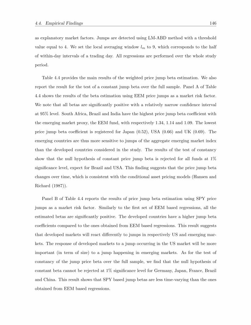
4.4. Empirical Findings 146
as explanatory market factors. Jumps are detected using LM-ABD method with a threshold
value equal to 4. We set the local averaging window lm to 9, which corresponds to the half
of within-day intervals of a trading day. All regressions are performed over the whole study
period.
Table 4.4 provides the main results of the weighted price jump beta estimation. We also
report the result for the test of a constant jump beta over the full sample. Panel A of Table
4.4 shows the results of the beta estimation using EEM price jumps as a market risk factor.
We note that all betas are significantly positive with a relatively narrow confidence interval
at 95% level. South Africa, Brazil and India have the highest price jump beta coefficient with
the emerging market proxy, the EEM fund, with respectively 1.34, 1.14 and 1.09. The lowest
price jump beta coefficient is registered for Japan (0.52), USA (0.66) and UK (0.69). The
emerging countries are thus more sensitive to jumps of the aggregate emerging market index
than the developed countries considered in the study. The results of the test of constancy
show that the null hypothesis of constant price jump beta is rejected for all funds at 1%
significance level, expect for Brazil and USA. This finding suggests that the price jump beta
changes over time, which is consistent with the conditional asset pricing models (Hansen and
Richard (1987)).
Panel B of Table 4.4 reports the results of price jump beta estimation using SPY price
jumps as a market risk factor. Similarly to the first set of EEM based regressions, all the
estimated betas are significantly positive. The developed countries have a higher jump beta
coefficients compared to the ones obtained from EEM based regressions. This result suggests
that developed markets will react differently to jumps in respectively US and emerging mar-
kets. The response of developed markets to a jump occurring in the US market will be more
important (in term of size) to a jump happening in emerging markets. As for the test of
constancy of the jump price beta over the full sample, we find that the null hypothesis of
constant beta cannot be rejected at 1% significance level for Germany, Japan, France, Brazil
and China. This result shows that SPY based jump betas are less time-varying than the ones
obtained from EEM based regressions.
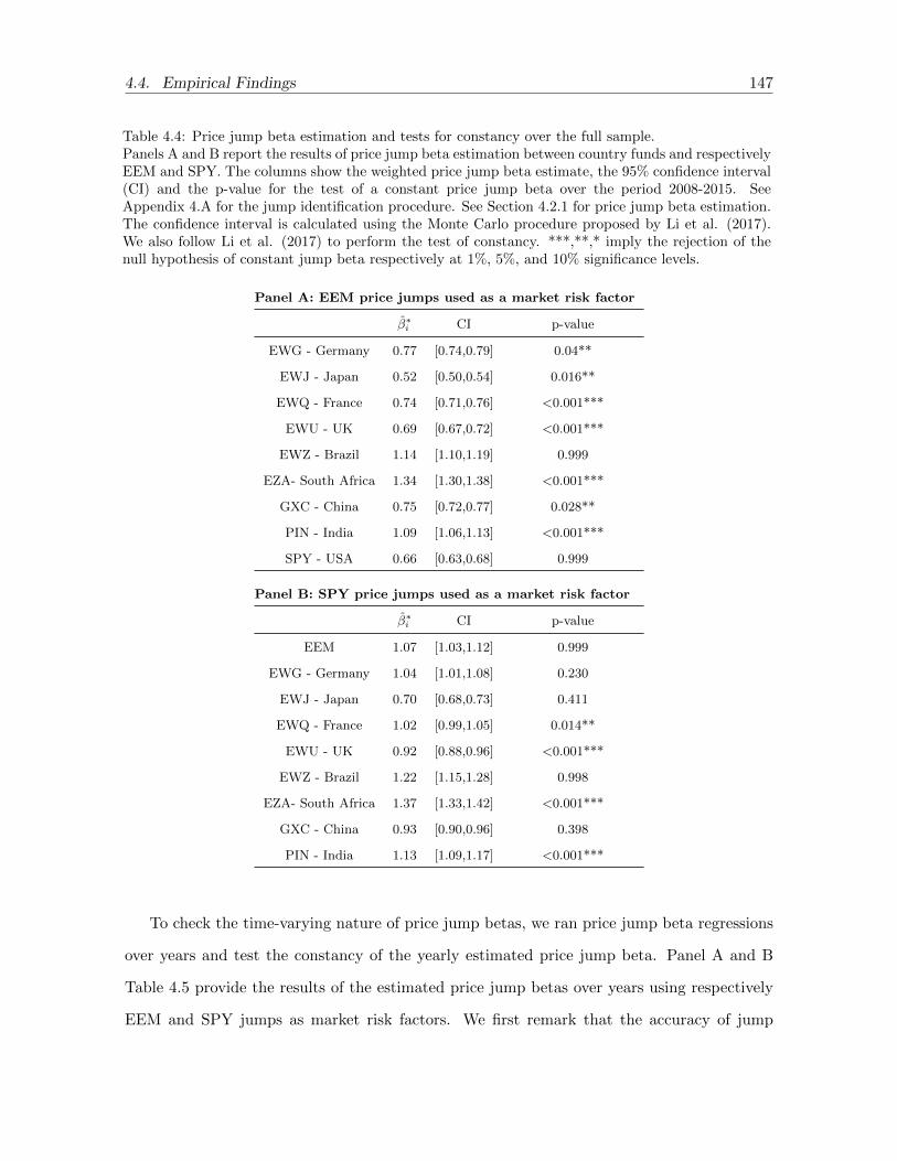
4.4. Empirical Findings 147
Table 4.4: Price jump beta estimation and tests for constancy over the full sample.Panels A and B report the results of price jump beta estimation between country funds and respectivelyEEM and SPY. The columns show the weighted price jump beta estimate, the 95% confidence interval(CI) and the p-value for the test of a constant price jump beta over the period 2008-2015. SeeAppendix 4.A for the jump identification procedure. See Section 4.2.1 for price jump beta estimation.The confidence interval is calculated using the Monte Carlo procedure proposed by Li et al. (2017).We also follow Li et al. (2017) to perform the test of constancy. ***,**,* imply the rejection of thenull hypothesis of constant jump beta respectively at 1%, 5%, and 10% significance levels.
Panel A: EEM price jumps used as a market risk factor
β∗i CI p-value
EWG - Germany 0.77 [0.74,0.79] 0.04**
EWJ - Japan 0.52 [0.50,0.54] 0.016**
EWQ - France 0.74 [0.71,0.76] <0.001***
EWU - UK 0.69 [0.67,0.72] <0.001***
EWZ - Brazil 1.14 [1.10,1.19] 0.999
EZA- South Africa 1.34 [1.30,1.38] <0.001***
GXC - China 0.75 [0.72,0.77] 0.028**
PIN - India 1.09 [1.06,1.13] <0.001***
SPY - USA 0.66 [0.63,0.68] 0.999
Panel B: SPY price jumps used as a market risk factor
β∗i CI p-value
EEM 1.07 [1.03,1.12] 0.999
EWG - Germany 1.04 [1.01,1.08] 0.230
EWJ - Japan 0.70 [0.68,0.73] 0.411
EWQ - France 1.02 [0.99,1.05] 0.014**
EWU - UK 0.92 [0.88,0.96] <0.001***
EWZ - Brazil 1.22 [1.15,1.28] 0.998
EZA- South Africa 1.37 [1.33,1.42] <0.001***
GXC - China 0.93 [0.90,0.96] 0.398
PIN - India 1.13 [1.09,1.17] <0.001***
To check the time-varying nature of price jump betas, we ran price jump beta regressions
over years and test the constancy of the yearly estimated price jump beta. Panel A and B
Table 4.5 provide the results of the estimated price jump betas over years using respectively
EEM and SPY jumps as market risk factors. We first remark that the accuracy of jump

4.4. Empirical Findings 148
beta estimates given by the 95% confidence level remains high. We also notice that yearly
estimated price jump betas seem to be less varying than full period estimates. Indeed, Table
4.6 shows that the rejection rate of the null hypothesis of constant beta over years at 5%
significance level represents 27% (39 rejections out of 144 regressions) of all yearly regressions
compared to 61% (11 rejections out of 18 regressions) for full sample regressions. In the same
way as for the full sample regressions, the rejection rate for SPY based regressions is lower
than EEM based regressions. One possible solution to improve the estimation of the remaining
time-varying betas is to further shorten the estimation period to six or three months.
Table 4.5: Price jump beta estimation over years.Panels A and B report the weighted price jump beta estimate (the 95% confidence interval is givenbetween brackets) for every fund and every year in the sample. The results are obtained using respec-tively EEM and SPY as market proxies. See Appendix 4.A for the jump identification procedure. SeeSection 4.2.1 for jump beta estimation. We follow Li et al. (2017) to provide confidence interval forthe weighted jump beta estimate.
Panel A: EEM price jumps used as a market risk factor
2008 2009 2010 2011
EWG 0.53 [0.47,0.58] 0.97 [0.85,1.08] 0.89 [0.82,0.96] 1.03 [0.96,1.11]
EWJ 0.48 [0.43,0.54] 0.54 [0.48,0.61] 0.59 [0.54,0.64] 0.58 [0.53,0.63]
EWQ 0.50 [0.44,0.55] 0.84 [0.74,0.94] 0.79 [0.74,0.84] 1.04 [0.95,1.12]
EWU 0.59 [0.52,0.66] 0.62 [0.54,0.70] 0.88 [0.80,0.95] 0.87 [0.80,0.94]
EWZ 1.29 [1.13,1.45] 1.07 [0.91,1.23] 1.17 [1.05,1.29] 1.13 [1.03,1.22]
EZA 0.78 [0.70,0.87] 1.06 [0.94,1.19] 1.46 [1.23,1.69] 1.08 [0.98,1.17]
GXC 0.81 [0.73,0.89] 0.96 [0.83,1.08] 0.60 [0.56,0.65] 0.95 [0.86,1.03]
PIN 0.60 [0.52,0.69] 0.68 [0.57,0.78] 1.63 [1.33,1.92] 0.66 [0.60,0.71]
SPY 0.67 [0.60,0.75] 0.76 [0.67,0.85] 0.66 [0.60,0.71] 0.80 [0.73,0.87]
2012 2013 2014 2015
EWG 0.95 [0.84,1.05] 0.58 [0.54,0.62] 0.62 [0.57,0.67] 0.82 [0.75,0.90]
EWJ 0.50 [0.44,0.56] 0.49 [0.44,0.54] 0.42 [0.37,0.46] 0.50 [0.44,0.55]
EWQ 1.01 [0.91,1.11] 0.60 [0.55,0.64] 0.66 [0.61,0.71] 0.82 [0.74,0.90]
EWU 0.79 [0.71,0.86] 0.51 [0.47,0.56] 0.52 [0.47,0.56] 0.64 [0.58,0.71]
EWZ 1.14 [1.01,1.26] 0.97 [0.90,1.03] 1.20 [1.10,1.29] 1.26 [1.15,1.37]
EZA 1.16 [1.03,1.30] 1.17 [1.08,1.26] 1.25 [1.15,1.34] 1.49 [1.36,1.62]
GXC 0.78 [0.70,0.86] 0.75 [0.70,0.80] 0.68 [0.62,0.73] 0.69 [0.62,0.77]
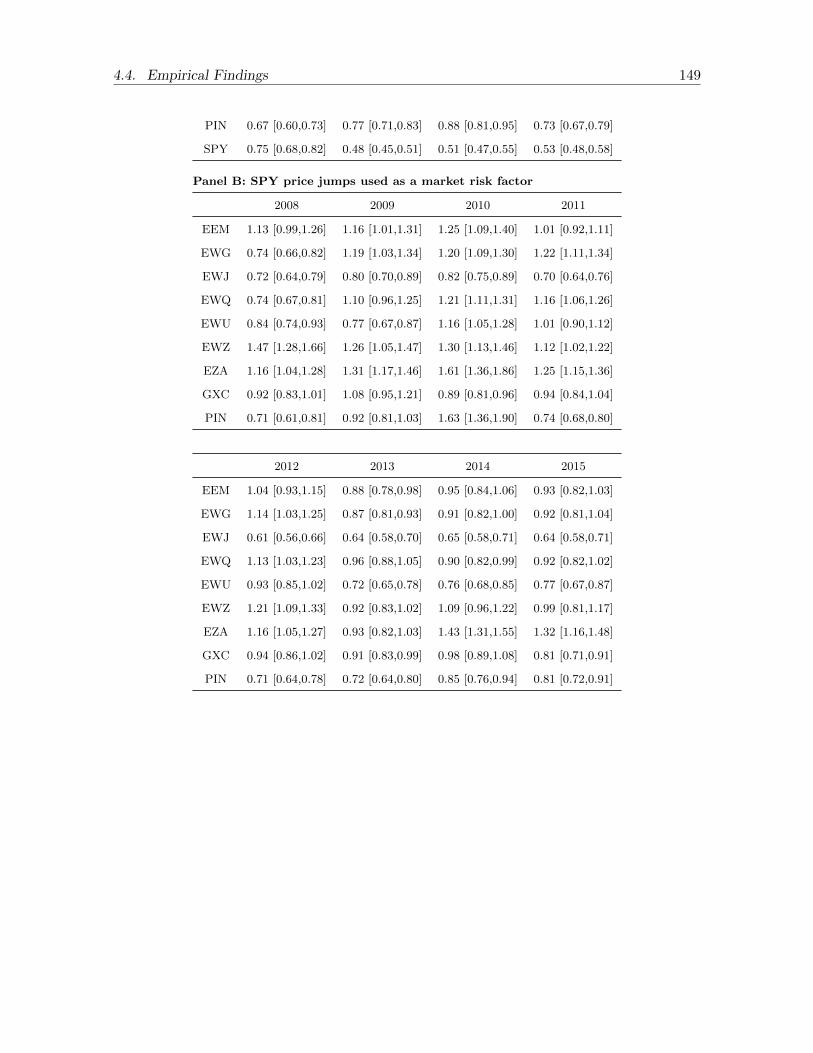
4.4. Empirical Findings 149
PIN 0.67 [0.60,0.73] 0.77 [0.71,0.83] 0.88 [0.81,0.95] 0.73 [0.67,0.79]
SPY 0.75 [0.68,0.82] 0.48 [0.45,0.51] 0.51 [0.47,0.55] 0.53 [0.48,0.58]
Panel B: SPY price jumps used as a market risk factor
2008 2009 2010 2011
EEM 1.13 [0.99,1.26] 1.16 [1.01,1.31] 1.25 [1.09,1.40] 1.01 [0.92,1.11]
EWG 0.74 [0.66,0.82] 1.19 [1.03,1.34] 1.20 [1.09,1.30] 1.22 [1.11,1.34]
EWJ 0.72 [0.64,0.79] 0.80 [0.70,0.89] 0.82 [0.75,0.89] 0.70 [0.64,0.76]
EWQ 0.74 [0.67,0.81] 1.10 [0.96,1.25] 1.21 [1.11,1.31] 1.16 [1.06,1.26]
EWU 0.84 [0.74,0.93] 0.77 [0.67,0.87] 1.16 [1.05,1.28] 1.01 [0.90,1.12]
EWZ 1.47 [1.28,1.66] 1.26 [1.05,1.47] 1.30 [1.13,1.46] 1.12 [1.02,1.22]
EZA 1.16 [1.04,1.28] 1.31 [1.17,1.46] 1.61 [1.36,1.86] 1.25 [1.15,1.36]
GXC 0.92 [0.83,1.01] 1.08 [0.95,1.21] 0.89 [0.81,0.96] 0.94 [0.84,1.04]
PIN 0.71 [0.61,0.81] 0.92 [0.81,1.03] 1.63 [1.36,1.90] 0.74 [0.68,0.80]
2012 2013 2014 2015
EEM 1.04 [0.93,1.15] 0.88 [0.78,0.98] 0.95 [0.84,1.06] 0.93 [0.82,1.03]
EWG 1.14 [1.03,1.25] 0.87 [0.81,0.93] 0.91 [0.82,1.00] 0.92 [0.81,1.04]
EWJ 0.61 [0.56,0.66] 0.64 [0.58,0.70] 0.65 [0.58,0.71] 0.64 [0.58,0.71]
EWQ 1.13 [1.03,1.23] 0.96 [0.88,1.05] 0.90 [0.82,0.99] 0.92 [0.82,1.02]
EWU 0.93 [0.85,1.02] 0.72 [0.65,0.78] 0.76 [0.68,0.85] 0.77 [0.67,0.87]
EWZ 1.21 [1.09,1.33] 0.92 [0.83,1.02] 1.09 [0.96,1.22] 0.99 [0.81,1.17]
EZA 1.16 [1.05,1.27] 0.93 [0.82,1.03] 1.43 [1.31,1.55] 1.32 [1.16,1.48]
GXC 0.94 [0.86,1.02] 0.91 [0.83,0.99] 0.98 [0.89,1.08] 0.81 [0.71,0.91]
PIN 0.71 [0.64,0.78] 0.72 [0.64,0.80] 0.85 [0.76,0.94] 0.81 [0.72,0.91]
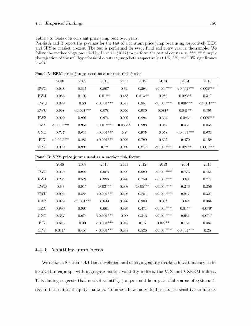
4.4. Empirical Findings 150
Table 4.6: Tests of a constant price jump beta over years.Panels A and B report the p-values for the test of a constant price jump beta using respectively EEMand SPY as market proxies. The test is performed for every fund and every year in the sample. Wefollow the methodology provided by Li et al. (2017) to perform the test of constancy. ***, **,* implythe rejection of the null hypothesis of constant jump beta respectively at 1%, 5%, and 10% significancelevels.
Panel A: EEM price jumps used as a market risk factor
2008 2009 2010 2011 2012 2013 2014 2015
EWG 0.948 0.515 0.897 0.61 0.294 <0.001*** <0.001*** 0.003***
EWJ 0.085 0.103 0.01** 0.488 0.013** 0.286 0.023** 0.817
EWQ 0.999 0.68 <0.001*** 0.619 0.851 <0.001*** 0.006*** <0.001***
EWU 0.998 <0.001*** 0.078 0.999 0.989 0.081* 0.041** 0.395
EWZ 0.999 0.992 0.974 0.999 0.994 0.314 0.096* 0.008***
EZA <0.001*** 0.959 0.001*** 0.036** 0.998 0.982 0.451 0.855
GXC 0.727 0.613 <0.001*** 0.8 0.935 0.978 <0.001*** 0.632
PIN <0.001*** 0.282 <0.001*** 0.993 0.799 0.635 0.479 0.159
SPY 0.999 0.999 0.72 0.999 0.877 <0.001*** 0.021** 0.001***
Panel B: SPY price jumps used as a market risk factor
2008 2009 2010 2011 2012 2013 2014 2015
EWG 0.999 0.999 0.988 0.999 0.999 <0.001*** 0.776 0.455
EWJ 0.204 0.528 0.996 0.994 0.759 <0.001*** 0.68 0.774
EWQ 0.99 0.917 0.003*** 0.098 0.005*** <0.001*** 0.236 0.259
EWU 0.995 0.884 <0.001*** 0.505 0.851 <0.001*** 0.947 0.327
EWZ 0.999 <0.001*** 0.649 0.999 0.989 0.07* 0.62 0.366
EZA 0.999 0.997 0.661 0.865 0.471 <0.001*** 0.01** 0.079*
GXC 0.337 0.674 <0.001*** 0.09 0.343 <0.001*** 0.631 0.071*
PIN 0.645 0.99 <0.001*** 0.949 0.15 0.029** 0.164 0.864
SPY 0.011* 0.457 <0.001*** 0.849 0.526 <0.001*** <0.001*** 0.25
4.4.3 Volatility jump betas
We show in Section 4.4.1 that developed and emerging equity markets have tendency to be
involved in cojumps with aggregate market volatility indices, the VIX and VXEEM indices.
This finding suggests that market volatility jumps could be a potential source of systematic
risk in international equity markets. To assess how individual assets are sensitive to market

4.4. Empirical Findings 151
volatility jumps, we assume that the individual asset volatility jumps are linked linearly to
jumps of the market volatility.
Table 4.7: Volatility jump beta estimation and tests for constancy over the full sample.Panels A and B report the results of volatility jump beta estimation between country funds andrespectively EEM and SPY. The columns show the quasi-maximum likelihood volatility jump betaestimate, the 95% confidence interval (CI) and the p-value for the test of a constant volatility jump betaover the period 2008-2015. See Appendix 4.A for the jump identification procedure. See Section 4.2.2for volatility jump beta estimation. We use the VXEEM and VIX volatility indices to approximate thejump arrival times of respectively EEM and SPY volatilities. The confidence intervals are calculatedusing the bootstrap procedure provided by Davies (2016). We also follow the methodology providedby Davies (2016) to perform the test of volatility jump beta constancy. ***,**,* imply the rejectionof the null hypothesis of constant volatility jump beta respectively at 1%, 5%, and 10% significancelevels.
Panel A: EEM volatility jumps used as a market risk factor
βvol,i CI p-value
EWG - Germany 0.58 [0.49,0.74] 0.015**
EWJ - Japan 0.44 [0.35,0.58] 0.562
EWQ - France 0.55 [0.45,0.71] 0.453
EWU - UK 0.56 [0.46,0.74] 0.582
EWZ - Brazil 0.72 [0.59,0.93] 0.996
EZA- South Africa 0.85 [0.49,1.26] <0.001***
GXC - China 0.42 [0.26,0.71] <0.001***
PIN - India 0.76 [0.61,0.97] <0.001***
SPY - USA 0.81 [0.70,0.97] 0.999
Panel B: SPY volatility jumps used as a market risk factor
βvol,i CI p-value
EEM 0.76 [0.72,0.88] 0.999
EWG - Germany 0.60 [0.55,0.70] 0.999
EWJ - Japan 0.46 [0.41,0.58] 0.993
EWQ - France 0.62 [0.57,0.76] 0.999
EWU - UK 0.61 [0.56,0.71] 0.999
EWZ - Brazil 0.52 [0.45,0.66] 0.046**
EZA- South Africa 0.57 [0.51,0.73] 0.003***
GXC - China 0.40 [0.31,0.59] <0.001***
PIN - India 0.72 [0.60,0.94] <0.001***

4.4. Empirical Findings 152
Panel A of Table 4.7 provides the results of volatility jump beta estimation for emerging
market volatility jumps. All regressions are performed over the full sample. We find that
all volatility jump betas are significantly positive for all countries in the sample. However,
the accuracy of the volatility jump beta estimates at 95% confidence level is lower than
the price jump beta estimates found in the previous subsection. The countries with highest
volatility jump betas with the EEM fund are South Africa (0.85), USA (0.81) and India
(0.76). The lowest volatility jump betas are found for China (0.42), Japan (0.44) and France
(0.55). The tests of constancy of the volatility jump beta show that the beta estimates are
time-varying especially for emerging countries. Panel B of Table 4.7 reports the results of
volatility jump beta estimation for all country funds with the SPY volatility jumps used as a
market risk factor. Similarly to EEM based regressions, all the SPY based volatility jump beta
estimates are significantly positive at 95% confidence level. The null hypothesis of constant
volatility jump beta is rejected for all emerging countries. The linear relationship between
developed markets and the US market seems to be more stable in time than with emerging
markets. When comparing between volatility jump beta estimates found for respectively SPY
and EEM, the results show that emerging countries are more sensitive to emerging market
volatility jumps than to US market volatility jumps. In contrast, the sensitivity of developed
countries to the SPY volatility jumps is higher than to emerging market volatility jumps.
Similarly to price jump beta estimates, we provide the results of volatility jump beta
estimation on year-by-year basis to make sure that our estimates are more stable in time for
a shorter estimation period. Panel A and B of Table 4.8 report the details of volatility jump
beta estimation for respectively EEM and SPY. We notice that the accuracy of estimates is
lower than the full sample case. However, the precision remains acceptable at 95% confidence
level. Table 4.9 provides the results of the test of volatility jump beta constancy over years.
The rejection rates dropped to 22% (10 out of 45 yearly regressions) and 19% (14 out of 72
yearly regressions) for respectively EEM and SPY based regressions compared to full sample
regressions where the rejection rate is 44% (4 out of 9 full sample regressions) at 5% significance
level.
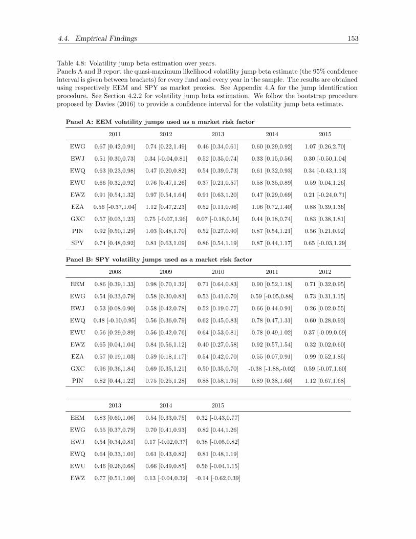
4.4. Empirical Findings 153
Table 4.8: Volatility jump beta estimation over years.Panels A and B report the quasi-maximum likelihood volatility jump beta estimate (the 95% confidenceinterval is given between brackets) for every fund and every year in the sample. The results are obtainedusing respectively EEM and SPY as market proxies. See Appendix 4.A for the jump identificationprocedure. See Section 4.2.2 for volatility jump beta estimation. We follow the bootstrap procedureproposed by Davies (2016) to provide a confidence interval for the volatility jump beta estimate.
Panel A: EEM volatility jumps used as a market risk factor
2011 2012 2013 2014 2015
EWG 0.67 [0.42,0.91] 0.74 [0.22,1.49] 0.46 [0.34,0.61] 0.60 [0.29,0.92] 1.07 [0.26,2.70]
EWJ 0.51 [0.30,0.73] 0.34 [-0.04,0.81] 0.52 [0.35,0.74] 0.33 [0.15,0.56] 0.30 [-0.50,1.04]
EWQ 0.63 [0.23,0.98] 0.47 [0.20,0.82] 0.54 [0.39,0.73] 0.61 [0.32,0.93] 0.34 [-0.43,1.13]
EWU 0.66 [0.32,0.92] 0.76 [0.47,1.26] 0.37 [0.21,0.57] 0.58 [0.35,0.89] 0.59 [0.04,1.26]
EWZ 0.91 [0.54,1.32] 0.97 [0.54,1.64] 0.91 [0.63,1.20] 0.47 [0.29,0.69] 0.21 [-0.24,0.71]
EZA 0.56 [-0.37,1.04] 1.12 [0.47,2.23] 0.52 [0.11,0.96] 1.06 [0.72,1.40] 0.88 [0.39,1.36]
GXC 0.57 [0.03,1.23] 0.75 [-0.07,1.96] 0.07 [-0.18,0.34] 0.44 [0.18,0.74] 0.83 [0.38,1.81]
PIN 0.92 [0.50,1.29] 1.03 [0.48,1.70] 0.52 [0.27,0.90] 0.87 [0.54,1.21] 0.56 [0.21,0.92]
SPY 0.74 [0.48,0.92] 0.81 [0.63,1.09] 0.86 [0.54,1.19] 0.87 [0.44,1.17] 0.65 [-0.03,1.29]
Panel B: SPY volatility jumps used as a market risk factor
2008 2009 2010 2011 2012
EEM 0.86 [0.39,1.33] 0.98 [0.70,1.32] 0.71 [0.64,0.83] 0.90 [0.52,1.18] 0.71 [0.32,0.95]
EWG 0.54 [0.33,0.79] 0.58 [0.30,0.83] 0.53 [0.41,0.70] 0.59 [-0.05,0.88] 0.73 [0.31,1.15]
EWJ 0.53 [0.08,0.90] 0.58 [0.42,0.78] 0.52 [0.19,0.77] 0.66 [0.44,0.91] 0.26 [0.02,0.55]
EWQ 0.48 [-0.10,0.95] 0.56 [0.36,0.79] 0.62 [0.45,0.83] 0.78 [0.47,1.31] 0.60 [0.28,0.93]
EWU 0.56 [0.29,0.89] 0.56 [0.42,0.76] 0.64 [0.53,0.81] 0.78 [0.49,1.02] 0.37 [-0.09,0.69]
EWZ 0.65 [0.04,1.04] 0.84 [0.56,1.12] 0.40 [0.27,0.58] 0.92 [0.57,1.54] 0.32 [0.02,0.60]
EZA 0.57 [0.19,1.03] 0.59 [0.18,1.17] 0.54 [0.42,0.70] 0.55 [0.07,0.91] 0.99 [0.52,1.85]
GXC 0.96 [0.36,1.84] 0.69 [0.35,1.21] 0.50 [0.35,0.70] -0.38 [-1.88,-0.02] 0.59 [-0.07,1.60]
PIN 0.82 [0.44,1.22] 0.75 [0.25,1.28] 0.88 [0.58,1.95] 0.89 [0.38,1.60] 1.12 [0.67,1.68]
2013 2014 2015
EEM 0.83 [0.60,1.06] 0.54 [0.33,0.75] 0.32 [-0.43,0.77]
EWG 0.55 [0.37,0.79] 0.70 [0.41,0.93] 0.82 [0.44,1.26]
EWJ 0.54 [0.34,0.81] 0.17 [-0.02,0.37] 0.38 [-0.05,0.82]
EWQ 0.64 [0.33,1.01] 0.61 [0.43,0.82] 0.81 [0.48,1.19]
EWU 0.46 [0.26,0.68] 0.66 [0.49,0.85] 0.56 [-0.04,1.15]
EWZ 0.77 [0.51,1.00] 0.13 [-0.04,0.32] -0.14 [-0.62,0.39]

4.4. Empirical Findings 154
EZA 0.56 [0.30,1.03] 0.58 [0.38,0.80] 0.16 [-0.86,0.78]
GXC 0.29 [-0.07,0.64] 0.25 [0.07,0.51] 0.45 [0.01,0.95]
PIN 0.46 [0.26,0.72] 0.51 [0.32,0.71] 0.49 [0.16,0.84]
Table 4.9: Tests of a constant volatility jump beta over years.Panels A and B report the p-values for the test of a constant volatility jump beta using respectivelyEEM and SPY as market proxies. The test is performed for every fund and every year in the sample.We use the VXEEM and VIX volatility indices to approximate the jump arrival times of respectivelyEEM and SPY volatilities. See Appendix 4.A for the jump identification procedure. We follow themethodology provided by Davies (2016) to perform the test of volatility jump beta constancy. ***,**,*imply the rejection of the null hypothesis of constant volatility jump beta respectively at 1%, 5%, and10% significance levels.
Panel A: EEM volatility jumps used as a market risk factor
2011 2012 2013 2014 2015
EWG 0.999 0.637 0.671 0.004*** <0.001***
EWJ 0.891 0.344 0.603 0.796 0.015**
EWQ 0.975 0.767 0.356 0.121 0.064*
EWU 0.999 0.902 0.24 0.064* 0.464
EWZ 0.999 0.984 0.84 0.983 0.101
EZA 0.609 0.056* <0.001*** 0.099* 0.91
GXC 0.088 <0.001*** <0.001*** 0.059* 0.035**
PIN 0.60 0.044** <0.001*** 0.004*** 0.987
SPY 0.999 0.999 0.425 0.23 0.661
Panel B: SPY volatility jumps used as a market risk factor
2008 2009 2010 2011 2012 2013 2014 2015
EEM 0.999 0.999 0.999 0.999 0.999 0.998 0.784 0.51
EWG 0.999 0.977 0.961 0.999 0.99 0.656 0.561 0.867
EWJ 0.932 0.991 0.737 0.999 0.807 0.92 0.093* 0.291
EWQ 0.344 0.999 0.958 0.995 0.984 0.008*** 0.712 0.976
EWU 0.803 0.998 0.999 0.999 0.553 0.625 0.988 0.535
EWZ 0.969 0.99 0.747 0.984 0.33 0.38 0.167 0.021**
EZA 0.271 0.026** 0.65 0.958 0.02 <0.001*** 0.158 0.021**
GXC 0.084 0.188 0.022** <0.001*** <0.001*** 0.007*** <0.001*** 0.637
PIN 0.28 <0.001*** <0.001*** 0.311 0.034** 0.027** 0.053* 0.834

4.4. Empirical Findings 155
4.4.4 Upside and downside jump betas
Several studies have documented that the correlation between international stock markets
exhibits asymmetric effects between positive and negative returns. In particular, the correla-
tion is higher for large down moves (see, among others, Longin and Solnik (2001), Ang and
Bekaert (2002), Ang and Chen (2002), Hartmann et al. (2004)). We also show in Section
4.4.1 that cojumps between asset returns and market volatilities are more frequent when re-
turns jump downward and volatilities jump upward. This result suggests that volatility jumps
are also asymmetric. This subsection examines whether the response of international stock
markets to upside and downside market jumps is asymmetric both at price and volatility
levels.
Table 4.10 reports the main proprieties of the estimated upside and downside price jump
betas. The betas are calculated for each country over the full sample using respectively
SPY and EEM funds as market proxies. Looking at the betas of developed and emerging
countries with the emerging market fund (EEM), we find that the downside price jump beta
is significantly higher than the upside one at 95% confidence level for Germany, France,
China and USA. On the opposite, the upside price jump beta is significantly greater than the
downside beta only for South Africa. Also, the null hypothesis of constant downside price
jump beta is rejected for seven countries at 95% significance level compared to only three
countries for the upside price jump beta, suggesting that the upside price jump betas are less
varying than downside ones over the sample period. As for the betas of the US market with
country funds considered in our study, we find that the difference between the downside and
upside price jump betas is significantly positive for Germany and France and significantly
negative for South Africa.
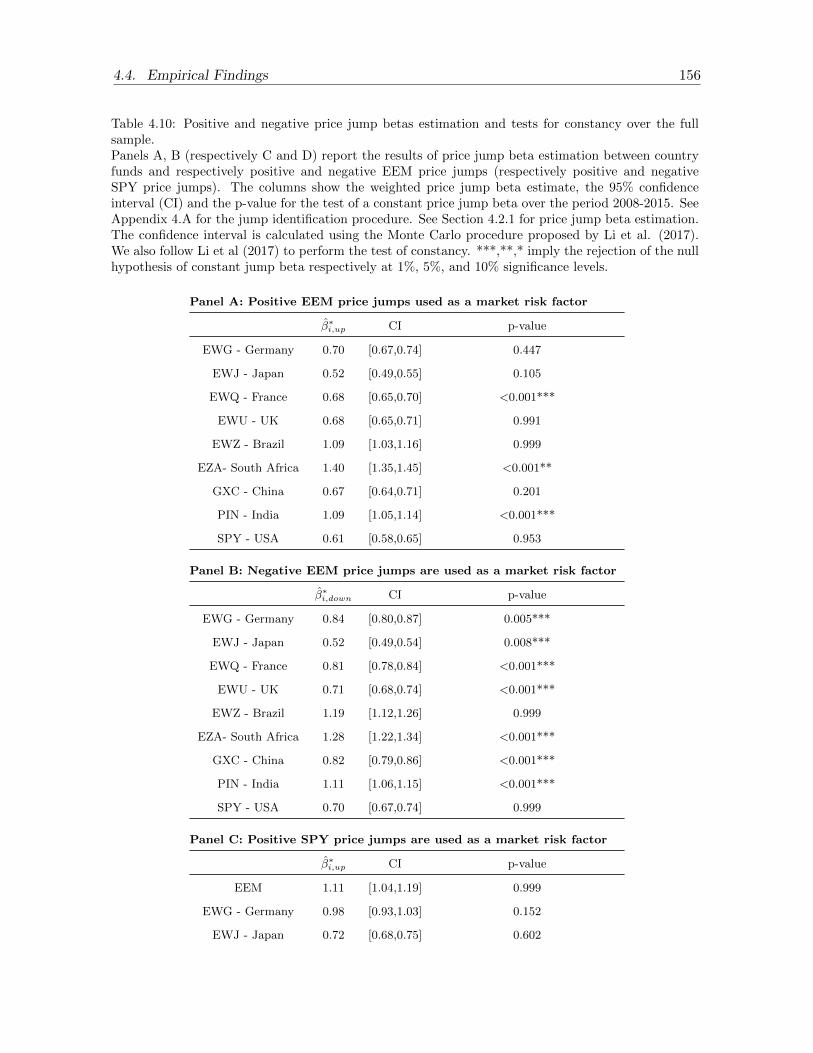
4.4. Empirical Findings 156
Table 4.10: Positive and negative price jump betas estimation and tests for constancy over the fullsample.Panels A, B (respectively C and D) report the results of price jump beta estimation between countryfunds and respectively positive and negative EEM price jumps (respectively positive and negativeSPY price jumps). The columns show the weighted price jump beta estimate, the 95% confidenceinterval (CI) and the p-value for the test of a constant price jump beta over the period 2008-2015. SeeAppendix 4.A for the jump identification procedure. See Section 4.2.1 for price jump beta estimation.The confidence interval is calculated using the Monte Carlo procedure proposed by Li et al. (2017).We also follow Li et al (2017) to perform the test of constancy. ***,**,* imply the rejection of the nullhypothesis of constant jump beta respectively at 1%, 5%, and 10% significance levels.
Panel A: Positive EEM price jumps used as a market risk factor
β∗i,up CI p-value
EWG - Germany 0.70 [0.67,0.74] 0.447
EWJ - Japan 0.52 [0.49,0.55] 0.105
EWQ - France 0.68 [0.65,0.70] <0.001***
EWU - UK 0.68 [0.65,0.71] 0.991
EWZ - Brazil 1.09 [1.03,1.16] 0.999
EZA- South Africa 1.40 [1.35,1.45] <0.001**
GXC - China 0.67 [0.64,0.71] 0.201
PIN - India 1.09 [1.05,1.14] <0.001***
SPY - USA 0.61 [0.58,0.65] 0.953
Panel B: Negative EEM price jumps are used as a market risk factor
β∗i,down CI p-value
EWG - Germany 0.84 [0.80,0.87] 0.005***
EWJ - Japan 0.52 [0.49,0.54] 0.008***
EWQ - France 0.81 [0.78,0.84] <0.001***
EWU - UK 0.71 [0.68,0.74] <0.001***
EWZ - Brazil 1.19 [1.12,1.26] 0.999
EZA- South Africa 1.28 [1.22,1.34] <0.001***
GXC - China 0.82 [0.79,0.86] <0.001***
PIN - India 1.11 [1.06,1.15] <0.001***
SPY - USA 0.70 [0.67,0.74] 0.999
Panel C: Positive SPY price jumps are used as a market risk factor
β∗i,up CI p-value
EEM 1.11 [1.04,1.19] 0.999
EWG - Germany 0.98 [0.93,1.03] 0.152
EWJ - Japan 0.72 [0.68,0.75] 0.602

4.4. Empirical Findings 157
EWQ - France 0.95 [0.91,0.99] 0.032**
EWU - UK 0.91 [0.86,0.97] 0.999
EWZ - Brazil 1.21 [1.12,1.30] 0.999
EZA- South Africa 1.50 [1.43,1.57] <0.001***
GXC - China 0.95 [0.90,1.00] 0.362
PIN - India 1.18 [1.13,1.23] <0.001***
Panel D: Negative SPY price jumps are used as a market risk factor
β∗i,down CI p-value EEM
EEM 1.04 [0.98,1.10] 0.999
EWG - Germany 1.10 [1.05,1.14] 0.578
EWJ - Japan 0.69 [0.66,0.73] 0.122
EWQ - France 1.08 [1.03,1.13] 0.23
EWU - UK 0.93 [0.88,0.97] <0.001***
EWZ - Brazil 1.23 [1.15,1.30] 0.708
EZA- South Africa 1.27 [1.20,1.34] <.001***
GXC - China 0.91 [0.87,0.96] 0.422
PIN - India 1.09 [1.04,1.14] <0.001***
Table 4.11 provides the results of the estimated upside and downside volatility jump betas
between country funds and respectively EEM and SPY volatility jumps. By comparing the
95% confidence interval of upside and downside beta estimates, we find that the difference
between two betas is not significant for almost all funds. The decomposition of the volatility
jump beta into upside and downside components reduces the total number of market volatility
jumps considered in the estimation of each beta, yielding to wider confidence levels for the
quasi-maximum likelihood estimates, especially for the downside volatility jump beta where
negative market volatility jumps are less frequent.
Overall, our findings suggest that international stock markets’ response to market price
jumps exhibit asymmetric effects between upside and downside components. The results of
the volatility jump beta decomposition into positive and negative components, however, are
not conclusive.

4.4. Empirical Findings 158
Table 4.11: Positive and negative volatility jump beta estimation and tests for constancy over the fullsample.Panels A and B (respectively C and D) report the results of volatility jump beta estimation betweencountry funds and respectively positive and negative EEM volatility jumps (respectively positive andnegative SPY volatility jumps). The columns show the quasi-maximum likelihood volatility jump betaestimate, the 95% confidence interval (CI) and the p-value for the test of a constant volatility jump betaover the period 2008-2015. See Appendix 4.A for the jump identification procedure. See Section 4.2.2for volatility jump beta estimation. We use the VXEEM and VIX volatility indices to approximate thejump arrival times of respectively EEM and SPY volatilities. The confidence intervals are calculatedusing the bootstrap procedure provided by Davies (2016). We also follow the methodology providedby Davies (2016) to perform the test of volatility jump beta constancy. ***,**,* imply the rejectionof the null hypothesis of constant volatility jump beta respectively at 1%, 5%, and 10% significancelevels.
Panel A: Positive EEM volatility jumps used as a market risk factor
βupvol,i CI p-value
EWG - Germany 0.63 [0.52,0.80] 0.109
EWJ - Japan 0.43 [0.32,0.59] 0.418
EWQ - France 0.61 [0.49,0.77] 0.826
EWU - UK 0.54 [0.41,0.71] 0.819
EWZ - Brazil 0.70 [0.56,0.92] 0.986
EZA- South Africa 0.95 [0.71,1.25] 0.166
GXC - China 0.23 [0.06,0.40] <0.001***
PIN - India 0.70 [0.58,0.97] 0.001***
SPY - USA 0.77 [0.65,0.91] 0.999
Panel B: Negative EEM volatility jumps used as a market risk factor
βdownvol,i CI p-value
EWG - Germany 0.48 [0.33,0.72] 0.041**
EWJ - Japan 0.45 [0.30,0.63] 0.634
EWQ - France 0.41 [0.22,0.63] 0.122
EWU - UK 0.60 [0.44,0.91] 0.185
EWZ - Brazil 0.74 [0.58,0.96] 0.925
EZA- South Africa 0.35 [-0.22,0.69] <0.001***
GXC - China 0.81 [0.59,1.17] 0.007***
PIN - India 0.87 [0.63,1.18] 0.014**
SPY - USA 0.88 [0.70,1.16] 0.716
Panel C: Positive SPY volatility jumps used as a market risk factor
βupvol,i CI p-value
EEM 0.72 [0.68,0.82] 0.999
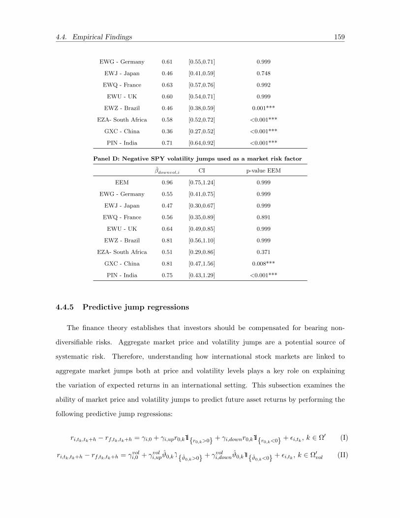
4.4. Empirical Findings 159
EWG - Germany 0.61 [0.55,0.71] 0.999
EWJ - Japan 0.46 [0.41,0.59] 0.748
EWQ - France 0.63 [0.57,0.76] 0.992
EWU - UK 0.60 [0.54,0.71] 0.999
EWZ - Brazil 0.46 [0.38,0.59] 0.001***
EZA- South Africa 0.58 [0.52,0.72] <0.001***
GXC - China 0.36 [0.27,0.52] <0.001***
PIN - India 0.71 [0.64,0.92] <0.001***
Panel D: Negative SPY volatility jumps used as a market risk factor
βdownvol,i CI p-value EEM
EEM 0.96 [0.75,1.24] 0.999
EWG - Germany 0.55 [0.41,0.75] 0.999
EWJ - Japan 0.47 [0.30,0.67] 0.999
EWQ - France 0.56 [0.35,0.89] 0.891
EWU - UK 0.64 [0.49,0.85] 0.999
EWZ - Brazil 0.81 [0.56,1.10] 0.999
EZA- South Africa 0.51 [0.29,0.86] 0.371
GXC - China 0.81 [0.47,1.56] 0.008***
PIN - India 0.75 [0.43,1.29] <0.001***
4.4.5 Predictive jump regressions
The finance theory establishes that investors should be compensated for bearing non-
diversifiable risks. Aggregate market price and volatility jumps are a potential source of
systematic risk. Therefore, understanding how international stock markets are linked to
aggregate market jumps both at price and volatility levels plays a key role on explaining
the variation of expected returns in an international setting. This subsection examines the
ability of market price and volatility jumps to predict future asset returns by performing the
following predictive jump regressions:
ri,tk,tk+h − rf,tk,tk+h = γi,0 + γi,upr0,k1r0,k>0 + γi,downr0,k1r0,k<0 + εi,tk , k ∈ Ω′ (I)
ri,tk,tk+h − rf,tk,tk+h = γvoli,0 + γvoli,upϑ0,k1ϑ0,k>0 + γvoli,downϑ0,k1ϑ0,k<0 + εi,tk , k ∈ Ω′vol (II)
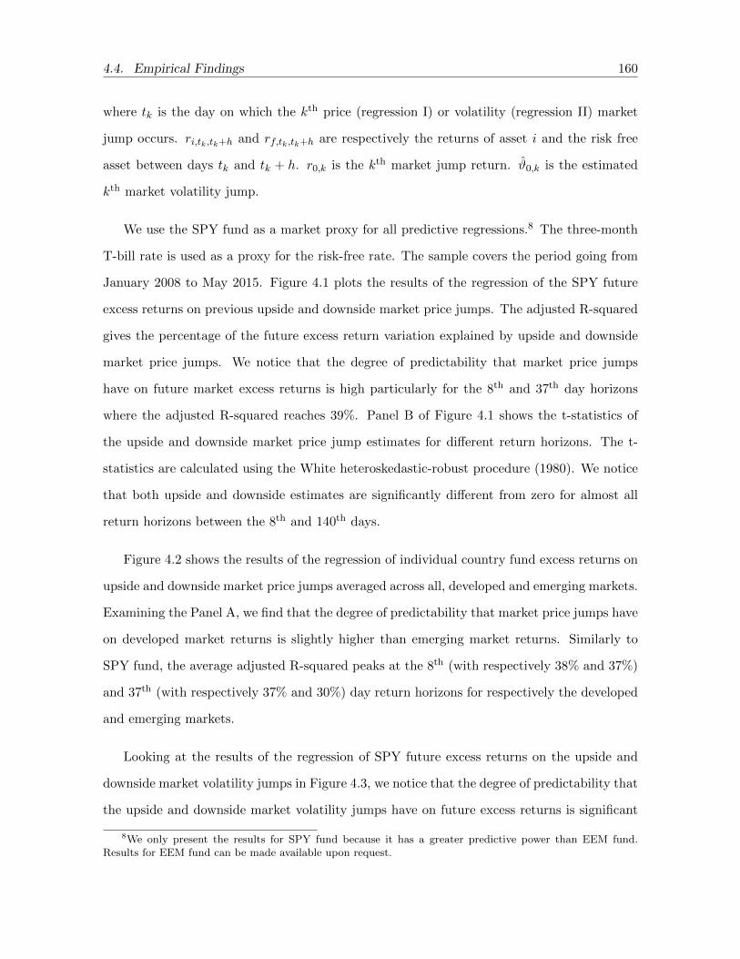
4.4. Empirical Findings 160
where tk is the day on which the kth price (regression I) or volatility (regression II) market
jump occurs. ri,tk,tk+h and rf,tk,tk+h are respectively the returns of asset i and the risk free
asset between days tk and tk + h. r0,k is the kth market jump return. ϑ0,k is the estimated
kth market volatility jump.
We use the SPY fund as a market proxy for all predictive regressions.8 The three-month
T-bill rate is used as a proxy for the risk-free rate. The sample covers the period going from
January 2008 to May 2015. Figure 4.1 plots the results of the regression of the SPY future
excess returns on previous upside and downside market price jumps. The adjusted R-squared
gives the percentage of the future excess return variation explained by upside and downside
market price jumps. We notice that the degree of predictability that market price jumps
have on future market excess returns is high particularly for the 8th and 37th day horizons
where the adjusted R-squared reaches 39%. Panel B of Figure 4.1 shows the t-statistics of
the upside and downside market price jump estimates for different return horizons. The t-
statistics are calculated using the White heteroskedastic-robust procedure (1980). We notice
that both upside and downside estimates are significantly different from zero for almost all
return horizons between the 8th and 140th days.
Figure 4.2 shows the results of the regression of individual country fund excess returns on
upside and downside market price jumps averaged across all, developed and emerging markets.
Examining the Panel A, we find that the degree of predictability that market price jumps have
on developed market returns is slightly higher than emerging market returns. Similarly to
SPY fund, the average adjusted R-squared peaks at the 8th (with respectively 38% and 37%)
and 37th (with respectively 37% and 30%) day return horizons for respectively the developed
and emerging markets.
Looking at the results of the regression of SPY future excess returns on the upside and
downside market volatility jumps in Figure 4.3, we notice that the degree of predictability that
the upside and downside market volatility jumps have on future excess returns is significant
8We only present the results for SPY fund because it has a greater predictive power than EEM fund.Results for EEM fund can be made available upon request.
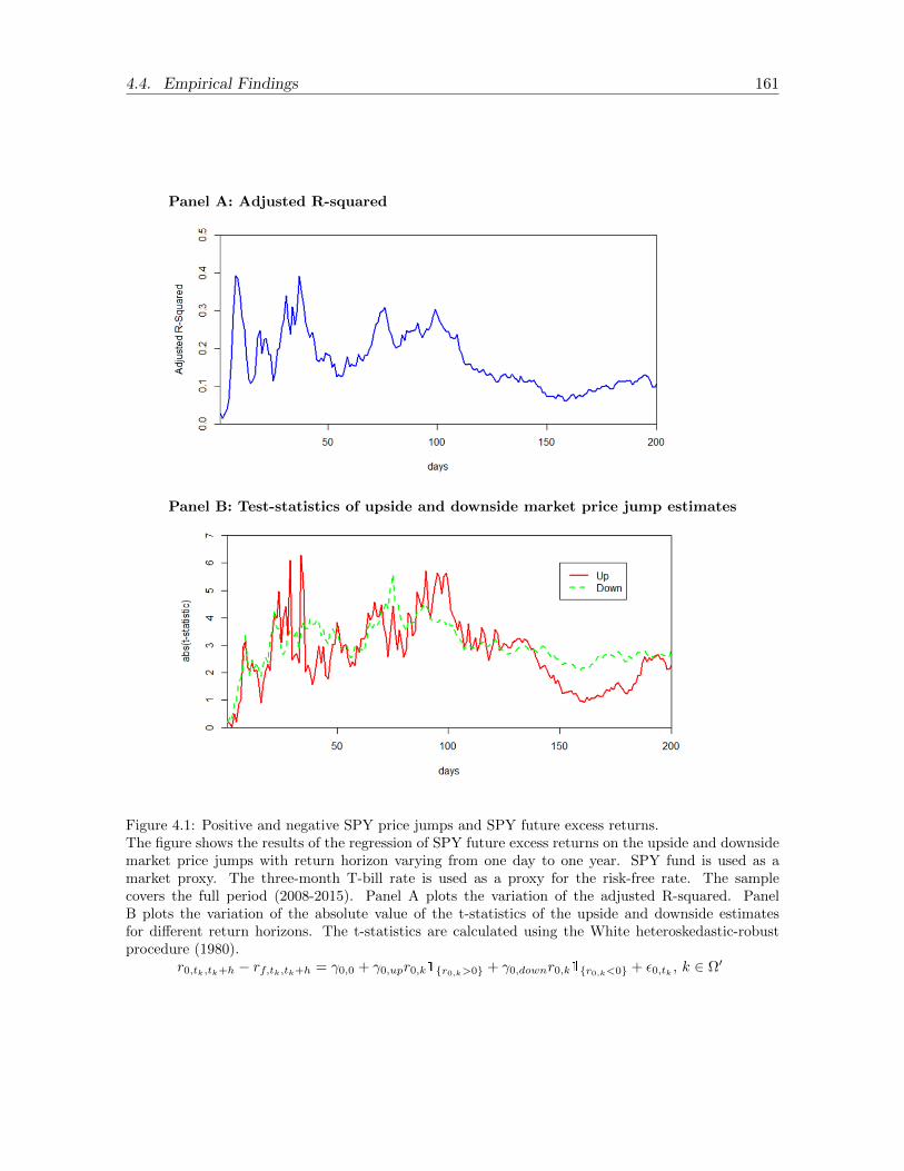
4.4. Empirical Findings 161
Panel A: Adjusted R-squared
Panel B: Test-statistics of upside and downside market price jump estimates
Figure 4.1: Positive and negative SPY price jumps and SPY future excess returns.The figure shows the results of the regression of SPY future excess returns on the upside and downsidemarket price jumps with return horizon varying from one day to one year. SPY fund is used as amarket proxy. The three-month T-bill rate is used as a proxy for the risk-free rate. The samplecovers the full period (2008-2015). Panel A plots the variation of the adjusted R-squared. PanelB plots the variation of the absolute value of the t-statistics of the upside and downside estimatesfor different return horizons. The t-statistics are calculated using the White heteroskedastic-robustprocedure (1980).
r0,tk,tk+h − rf,tk,tk+h = γ0,0 + γ0,upr0,k1r0,k>0 + γ0,downr0,k1r0,k<0 + ε0,tk , k ∈ Ω′

4.4. Empirical Findings 162
Panel A: Adjusted R-squared
Figure 4.2: Positive and negative SPY price jumps and future individual country fund excess returns.The figure shows the results of the regression of future individual country fund excess returns on theupside and downside market price jumps with return horizon varying from one day to one year. SPYfund is used as a market proxy. The three-month T-bill rate is used as a proxy for the risk-free rate.The sample covers the full period (2008-2015). Panel A plots the variation of the adjusted R-squaredaveraged respectively across all, developed and emerging funds considered in the study. Panels Band C plot the variation of the absolute value of the t-statistics of the upside and downside estimatesaveraged respectively across all, developed and emerging funds considered in the study. The t-statisticsare calculated using the White heteroskedastic-robust procedure (1980).
ri,tk,tk+h − rf,tk,tk+h = γi,0 + γi,upr0,k1r0,k>0 + γi,downr0,k1r0,k<0 + εi,tk , k ∈ Ω′
between the 6th and 70th day horizons. It peaks at the 28th day horizon with an adjusted
R-squared around 6%. Panel B of Figure 4.3 shows that the upside volatility jump estimates
are significant for almost all horizons between the 6th and 70th days whereas the downside
volatility jump estimates are only significant for a few horizons around the 28th day. Looking
at the aggregated results for all, developed and emerging markets in Figure 4.4, we find that
the regression estimates are only significant for developed markets, where the adjusted R-
squared varies between 2% and 4.5%. This finding shows that the predictive power of market
volatility jumps is weak compared to market price jumps.
Overall, the results of the predictive regressions indicate that both price and volatility
market jumps have a significant degree of predictability on future excess returns especially at
one to four month horizon. However, the proportion of future return variation explained by
market price jumps is much greater than that explained by market volatility jumps.

4.4. Empirical Findings 163
Panel B: Test-statistics of the upside market price jump estimates
Panel C: Test-statistics of the downside market price jump estimates
(Figure 4.2)

4.4. Empirical Findings 164
Panel A: Adjusted R-squared
Panel B: Test-statistics of the upside and downside market volatility jump estimates
Figure 4.3: Positive and negative SPY volatility jumps and SPY future excess returns.The figure shows the results of the regression of SPY future excess returns on the upside and downsidemarket volatility jumps with return horizon varying from one day to one year. SPY fund is used asa market proxy. The three-month T-bill rate is used as a proxy for the risk-free rate. The samplecovers the full period (2008-2015). Panel A plots the variation of the adjusted R-squared. PanelB plots the variation of the absolute value of the t-statistics of the upside and downside estimatesfor different return horizons. The t-statistics are calculated using the White heteroskedastic-robustprocedure (1980).
r0,tk,tk+h − rf,tk,tk+h = γvol0,0 + γvol0,upϑ0,k1ϑ0,k>0 + γvol0,downϑ0,k1ϑ0,k<0 + ε0,tk , k ∈ Ω′vol

4.4. Empirical Findings 165
Panel A: Adjusted R-squared
Figure 4.4: Positive and negative SPY volatility jumps and future individual country fund excessreturns.The figure shows the results of the regression of future individual country fund excess returns on theupside and downside market volatility jumps with return horizon varying from one day to one year.SPY fund is used as a market proxy. The three-month T-bill rate is used as a proxy for the risk-freerate. The sample covers the full period (2008-2015). Panel A plots the variation of the adjustedR-squared averaged respectively across all, developed and emerging funds considered in the study.Panels B and C plot the variation of the absolute value of the t-statistics of the upside and downsideestimates averaged respectively across all, developed and emerging funds considered in the study. Thet-statistics are calculated using the White heteroskedastic-robust procedure (1980).
ri,tk,tk+h − rf,tk,tk+h = γvoli,0 + γvoli,upϑ0,k1ϑ0,k>0 + γvoli,downϑ0,k1ϑ0,k<0 + εi,tk , k ∈ Ω′vol

4.4. Empirical Findings 166
Panel B: Test-statistics of the upside market volatility jump estimates
Panel C: Test-statistics of the downside market volatility jump estimates
(Figure 4.4)

4.5. Conclusion 167
4.5 Conclusion
In this paper, we examine the relationship between international stock markets and jumps
of an aggregate risk factor both at price and volatility levels. By considering a sample covering
major developed and emerging stock markets, we measure the sensitivity of each individual
stock market to price and volatility jumps of an aggregate market proxy, and document that
these betas are time-varying over the sample period and exhibit asymmetric effects across
upside and downside market movements. By applying the techniques proposed by Andersen
et al. (2007) and Lee and Mykland (2008), we identify all intraday jumps and cojumps of
all stock markets and volatility indices (VIX and VXEEM) in the sample and we find that
cojumps between individual country funds and two volatility indices have opposite signs,
with a higher proportion of positive volatility and negative return cojumps, suggesting a
strong anti-correlation between market volatility jumps and asset returns when the market is
downward and its volatility is high.
Finally, we consider predictive regressions of future international stock market returns on
upside and downside price and volatility market jumps and document that both price and
volatility market jumps have a significant predictive power on future stock market returns,
with a greater predictability degree found for market price jumps.
The findings of this study show that market price and volatility jump risks are likely to
be derived by common underlying risk factors. Given the dependency between two risks,
providing suitable hedging strategies for price and volatility jumps is a challenging issue for
both practitioners and researchers. Studying the role of systematic price and volatility jumps
in forecasting the market volatility is also an interesting topic for future research.

References
Aıt-Sahalia, Y. and J. Jacod (2009). Testing for Jumps in a Discretely Observed Process.
Annals of Statistics 37, 184-222.
Aıt-Sahalia, Y. and J. Jacod (2011). Testing whether jumps have finite or infinite activity.
Annals of Statistics 39, 1689-1719.
Alexeev,V., Dungey, M. and Yao, W., 2017. Time-varying continuous and jump betas: The
role of firm characteristics and periods of stress. Journal of Empirical Finance 20, 1-20.
Andersen, T.G, Bollerslev, T., and Dobrev, D., 2007. No-arbitrage semi-martingale restric-
tions for continuous-time volatility models subject to leverage effects, jumps and i.i.d. noise:
Theory and testable distributional implications. Journal of Econometrics 138 (1), 125-180.
Ang, A., and Bekaert, G., 2002. International Asset Allocation with Regime Shifts. Review
of Financial Studies 15, 1137-1187.
Ang, A. and Chen, J., 2002. Asymmetric correlations of equity portfolios. Journal of Financial
Economics 63, 443-494.
Ang, A., Hodrick, R., Xing, Y., and Zhang, X., 2006. The cross-section of volatility and
expected returns, Journal of Finance 61, 259-299.
Bae, K.H., Karolyi, G.A., and Stulz, R., 2003. A new approach to measuring financial conta-
gion. Review of Financial Studies 16, 717-763.
Bandi, F.M., and Reno, R. 2016. Price and volatility co-jumps. Journal of Financial Economics
119, 107-146.
Barndorff-Nielsen O. E. and Shephard, N., 2004. Power and bipower variation with stochastic
volatility and jumps. Journal of Financial Econometrics 2, 1-37.
Barndorff-Nielsen, O. E. and Shephard, N., 2006. Econometrics of testing for jumps in financial
economics using bipower variation. Journal of Financial Econometrics 4, 1-30.
168

REFERENCES 169
Bekaert, G., Erb, C., Harvey, C., Viskanta, T., 1998. The distributional characteristics of
emerging market returns and asset allocation. Journal of Portfolio Management 24 (2),
102-116.
Broadie, M., M. Chernov, and M. Johannes (2007). Specification and Risk Premiums: The
Information in S&P 500 Futures Options. Journal of Finance 62.
Bollerslev, T., Law, T. H., Tauchen, G., 2008. Risk, jumps, and diversification. Journal of
Econometrics 144 (1), 234-256.
Bollerslev T., Todorov V., and Li S. Z., 2016, Roughing up Beta: continuous vs. discontinuous
betas, and the cross-section of expected stock returns. Journal of Financial Economics 120
(3), 464-490.
Chernov, M., R. Gallant, E. Ghysels, and G. Tauchen (2003). Alternative Models for Stock
Price Dynamics. Journal of Econometrics 116, 225-257.
Cremers, M., Halling, M. and Weinbaum, D., 2015. Aggregate Jump and Volatility Risk in
the Cross-Section of Stock Returns. The Journal of Finance 70 (2), 577- 614.
Davies, R., 2016. Volatility Jump Regressions. Working paper, Duke university.
Duffie, D., J. Pan, and K. Singleton (2000). Transform Analysis and Asset Pricing for Affine
Jump- Diffusions. Econometrica 68, 1343-1376.
Eraker, B., 2004. Do Stock Prices and Volatility Jump? : Reconciling Evidence from Spot
and Option Prices. Journal of Finance 59, 1367-1403.
Eraker, B., M. Johannes, and N. Polson, 2003. The Impact of Jumps in Volatility and Returns.
Journal of Finance 58, 1269-1300.
Hansen, L. P., and Richard, S. F., 1987. The Role of Conditioning Information in Deducing
Testable Restrictions Implied by Dynamic Asset Pricing Models, Econometrica 55, 587-613.
Jacod, J., Todorov, V., 2010. Do price and volatility jump together? The Annals of Applied
Probability 20, 1425-69.

REFERENCES 170
Harris, L., 1986. A transaction data study of weekly and intradaily patterns in stock returns.
Journal of Financial Economics 16, 99-117.
Hartmann, P., Straetmans, S. and de Vries, C., 2004. Asset market linkages in crisis periods.
Review of Economics and Statistics 86, 313-326.
Li, J., Todorov, V., Tauchen, G., 2017. Jump Regressions. Econometrica 85, 173-195.
Lee S. S. and Mykland, P.A., 2008. Jumps in financial markets: A new nonparametric test
and jump dynamics. Review of Financial Studies 21, 2535-2563.
Longin, F., and Solnik B., 2001, Extreme Correlation of International Equity Markets. Journal
Finance 56, 649-676.
Oordt, M and Zhou, C., 2016. Systematic tail risk. Journal of Financial and Quantitative
Analysis 51, 685-705.
Todorov, V., Tauchen, G., 2011.Volatility jumps. Journal of Business and Economic Statistics
29, 356-371.
Weigert, F., 2016. Crash Aversion and the Cross-Section of Expected Stock Returns World-
wide. The Review of Asset Pricing Studies 6, 135-178.
White, H., 1980. A Heteroskedasticity-Consistent Covariance Matrix Estimator and a Direct
Test for Heteroskedasticity. Econometrica 48 (4), 817-838.
Wood, R, A., McInish, A., Thomas H., and Ord, K., 1985. An investigation of transaction
data for NYSE stocks. Journal of Finance 40, 723-741.

4.A. Jump and cojump identification methodology 171
Appendix 4.A Jump and cojump identification methodology
LM-ABD jump identification test
The LM test statistic Lt,k compares the current asset return with the bipower variation
calculated over a moving window with a given number of preceding observations. It tests at
time k on day t whether there was a jump from k − 1 to k and is defined as follows:
Lt,k =|rt,k|σt,k
where
σ2t,k =
1
K − 2
k−1∑j=k−K+2
|rt,j−1| |rt,j |
rt,k is the intraday return in the interval [k−1, k] of day t. σt,k refers to the realized bipower
variation calculated for a window of K observations and provides a jump robust estimator
of the instantaneous volatility. Lee and Mykland (2008) emphasize that the window size K
should be chosen in a way that the effect of jumps on the volatility estimation disappears.
They thus suggest to choose the window size K between√
252×M and 252×M , where M
is the number of observations in a day. Under the null hypothesis of absence of jumps at
anytime in the interval [k − 1, k], the LM statistic is asymptotically distributed as follows:
Lt,k − CMSM
M→∞−−−−→ ξ
where ξ has a cumulative distribution function, P (ξ ≤ x) = exp(e−x). CM and SM are given
by:
CM =
√2 log(M)
c−√
log(π) + log(log(M))
2c√
2 log(M)
SM =1
c√
2 log(M)and c =
√2
π
A jump is detected with LM test on day t in intraday interval k if the following condition

4.A. Jump and cojump identification methodology 172
is satisfied:
|Lt,k|> − log(− log(1− α))× SM + CM
where α is the test significance level.
On the other hand, the ABD test statistic is assumed to be normally distributed in the
absence of jumps. A jump is detected with the ABD test on day t in intraday interval k if
the following condition is satisfied:
|rt,k|√1MBV t
> Φ−1
1−β2
where BV t is the bipower variation (Barndorff-Nielsen and Shephard 2004) defined as follows:
BV t =π
2
M
M − 1
M∑k=2
|rt,k−1| |rt,k−1|
Φ−1
1−β2
represents the inverse of the standard normal cumulative distribution function eval-
uated at a cumulative probability of 1− β2 and (1−β)M = 1−α, where α represents the daily
significance level of the test.
In our study, we identify intraday jumps by relying on the intraday procedure of LM-ABD.
A jump is detected with the LM-ABD test on day t in intraday interval k when:
|rt,k|σt,k
> θ
The threshold value θ is calculated for different significance levels. For a daily significance
level of 5% and a sampling frequency of 20 minutes (which corresponds to 19 intraday returns
per day in our study), we obtain a threshold value of 4.00 and 4.85 using ABD and LM
methods, respectively.

4.A. Jump and cojump identification methodology 173
Cojump identification test
Once all intraday jumps are identified using the univariate jump detection test of LM-
ABD, we apply the following co-exceedance rule to verify if a cojump occurs between assets
i and j at intraday time k on day t (Bae et al., 2003):
1 |ri,t,k|σi,t,k
>θ
× 1 |rj,t,k|σj,t,k
>θ
=
1 : a cojump between assets i and j
0 : no cojump
Thus, a cojump exists when asset returns jump simultaneously. We distinguish between
an idiosyncratic jump defined as jump of a single asset or jump that occurs independently
of the market movement and cojump defined as jumps of two or more assets that occur
simultaneously.
Intraday volatility pattern
It is widely documented (Wood et al. (1985) and Harris (1986)) that intraday returns
show a systematic seasonality over the trading day, also called the U-shaped pattern. The
intraday volatility is particularly higher at the open and the close of the trading than the
rest of the day. To minimize the effects of intraday volatility on our jump detection test, we
modify our procedure by rescaling intraday returns with a volatility jump robust corrector
introduced by Bollerslev et al. (2008). The kth rescaled intraday return of day t is defined
by:
rt,k =rt,kςk

4.A. Jump and cojump identification methodology 174
where:
ς21 =
M
T∑t=1
|rt,1| |rt,2|
T∑t=1
|rt,1| |rt,2|+T∑t=1
M−1∑l=2
|rt,l−1|12 |rt,l| |rt,l+1|
12 +
T∑t=1
|rt,M−1| |rt,M |
ς2k =
M
T∑t=1
|rt,k−1|12 |rt,k| |rt,k+1|
12
T∑t=1
|rt,1| |rt,2|+T∑t=1
M−1∑l=2
|rt,l−1|12 |rt,l| |rt,l+1|
12 +
T∑t=1
|rt,M−1| |rt,M |
, k = 2, . . . ,M − 1
ς2M =
M
T∑t=1
|rt,M−1| |rt,M |
T∑t=1
|rt,1| |rt,2|+T∑t=1
M−1∑l=2
|rt,l−1|12 |rt,l| |rt,l+1|
12 +
T∑t=1
|rt,M−1| |rt,M |
T is the total number of days considered in the study and M is the number of observations
in a day.


Chapter 5
General Conclusion
Over the past four decades, the topic of international stock market interdependencies has been
extensively studied in the finance literature. The issue has received increasing attention due
to the recurrence of financial crises that occurred in both developed and emerging countries
during the last decades. Indeed, understanding the nature of cross-market correlations in pe-
riod of financial and economic turmoil is of great interest for both investors and policy makers
who want to guard against the contagion risk. Moreover, the increased market integration
that has experienced developed and emerging markets has led the researchers to question
whether the benefits of international diversification are disappearing over time.
More recently, more attention has been given to the extreme comovement of international
stock markets in the finance literature. The study of the tail dependence structure of inter-
national equity market returns was made possible thanks to the availability of high frequency
data. It was also boosted by the development of numerous econometrical tools that help
researchers to examine the dependence between extreme market variations. This thesis con-
tributes to the existing literature by studying cojumps in international equity markets and
assessing their impact on portfolio allocation decisions and asset pricing.
In the second chapter, we empirically investigate the dynamics of cojumps between inter-
national equity markets and show their impact on international asset allocation and portfolio
diversification benefits. Our empirical work relies on the use of intraday returns for three
international exchange-traded funds, SPY, EFA, and EEM, which are used to capture the
performance of respectively the US, developed countries (excluding the US and Canada) and
emerging equity markets. The data covers the period going from January 2008 to October
2013. We apply the jump identification test of Lee and Mykland (2008) to identify all intra-
day jumps and cojumps of the three funds over the sample period. We find that the number
176

177
of detected intraday jumps is higher in developed markets (US and EFA) than in emerging
markets, suggesting a higher degree of asset comovement within developed markets. We also
show that cojumps between the US market and other developed markets are higher than
cojumps between the US and emerging markets.
We examine the time and space clustering features of jumps across international markets
using a bivariate Hawkes model (1971) and provide evidence of an asymmetric jump trans-
mission between markets with a stronger transmission from the US market to other developed
and emerging markets. The transmission of jumps in the other way around is also significant
but the strength is weaker.
To assess the impact of cojumps on portfolio allocation decisions, we consider a domestic
US investor who selects his portfolio composition based on two assets, a domestic risky asset
(SPY) and two foreign risky assets (EFA and EEM), in a way to minimize the portfolio’s risk.
We use the mean-variance and mean-CVaR approaches to determine the optimal portfolio
composition and analyze how the demand of foreign assets varies with cojump intensity. We
provide strong evidence of a significant negative relationship between the optimal propor-
tion of foreign assets and cojumps between domestic and foreign assets. This result implies
that domestic US investors allocate more money towards home assets in the presence of co-
jumps between US and foreign markets. We also investigate the role of higher-order moments
induced by intraday jumps on international diversification. For this purpose, we consider
an investor who recognizes idiosyncratic and systematic jumps and assumes a multivariate
jump-diffusion process for asset returns and another investor who ignores jumps and assumes
a pure multivariate diffusion process for asset returns. Both investors have the same power
utility function. Our results show that optimal portfolio weights are almost the same for the
pure-diffusion and jump-diffusion investors. The impact of jump higher-order moments on
the optimal portfolio composition is thus insignificant.
In the third chapter, we examine the pricing of systematic continuous and jump risks
in the cross-section of international stock returns by considering a general pricing framework

178
involving six separate market risk factors. We first decompose the systematic market risk into
intraday and overnight components. The intraday market risk includes both continuous and
jump parts. We then consider the asymmetry and size effects of market jumps by separating
the systematic jump risk into positive vs. negative and small vs. large components. Our
empirical investigation relies on the use of the intraday data of a set of 37 country exchange-
traded funds covering developed, emerging and frontier markets from July 2003 to December
2014. By considering the cojumps of individual country markets with an aggregate market
index, we find that jumps in developed countries are more linked to the aggregate market
index than emerging and frontier markets. We also show that jumps in Asian stock markets
are more linked to the aggregate index than other emerging markets in the sample, suggesting
that investors investing in non-Asian emerging markets may better minimize their exposure
to systematic jump risk.
We apply Todorov and Bollerslev’s (2010) methodology to estimate the exposure of each
country fund returns towards the systematic market diffusive and jump risks and show that in-
dividual country funds are more sensitive to discontinuous market movements than to smooth
ones. The small jump beta is, on average, greater than large jump beta indicating that coun-
try funds are more sensitive to small frequent market jumps than large infrequent market
jumps. We also show that the downside jump beta is, on average, highest among all betas
suggesting country funds react to unexpected negative information arrival the most.
The results of portfolio sorting approach and the cross-sectional Fama and MacBeth (1973)
regressions show continuous and downside discontinuous risks are positively rewarded in the
cross-section of expected stock returns during the pre-crisis period whereas the upside and
large jump risks are negatively priced during the crisis and post-crisis periods, suggesting that
investors prefer stocks that help them hedge against large movements of the market during
the crisis period. By considering the relationship between asset prices and the volatility, we
provide evidence of significant continuous and downside jump leverage effects during the pre-
crisis period, indicating that both price and volatility risks share compensations for common
underlying risk factors during the pre-crisis period.

179
In the fourth chapter, we tackle the issue of pricing of systematic price and volatility jump
risks by examining the response of developed and emerging markets to jumps of an aggregate
market index both at price and volatility levels. Our empirical investigation is based on two
sets of high frequency data. The first set is composed of ten country exchange-traded funds
covering major developed and emerging markets from January 2008 to May 2015. The second
set is composed of two volatility indices: The Chicago Board of Options Exchange’s (CBOE)
Volatility Index (VIX) and CBOE Emerging Markets ETF Volatility Index (VXEEM) serv-
ing as proxies for respectively the developed and emerging market volatilities. We apply the
method of Lee and Mykland (2008) to identify intraday jumps and cojumps between individ-
ual country funds and volatility indices. We show that the discontinuous downside changes in
prices are often associated with strongly anti-correlated, contemporaneous, discontinuous up-
side changes in volatility, suggesting that both the price and volatility jump risks are derived
by common underlying risk factors and thus should be handled jointly by investors.
By applying the jump regression procedures proposed by Li et al. (2017) and Davies
(2016), we estimate the sensitivity of developed and emerging countries to respectively market
price and volatility jumps and document that both price and volatility jump betas are time-
varying over the sample period. We also study the exposure of individual country markets to
upside and downside price and volatility jumps of the aggregate market index and document
that international stock markets’ response to market price jumps exhibits asymmetric effects
between upside and downside components. In contrast, the results of the volatility jump
beta decomposition into upside and downside components are not conclusive. Finally, we
examine the role of price and volatility market jumps in forecasting future excess returns of
international stock markets and find that both price and volatility market jumps have a signif-
icant predictive power on future stock market returns, with a greater degree of predictability
obtained with market price jumps.
This dissertation opens interesting avenues for future research. It would be interesting to
investigate if the negative relationship between the demand of foreign assets and the intensity
of cojumps between domestic and foreign markets could be generalized, in addition to the US

180
market, to other developed and emerging markets. It would be also of interest to examine the
underlying mechanisms of price and volatility cojumps. Future studies could further examine
whether exchange-traded funds are a good proxy for their underlying indices. Studying the
implications of the pricing frameworks proposed in the second and third essays on the portfolio
value-at-risk calculation as well as the simultaneous hedging of price and volatility jump risks
are also of great interest for both practitioners and researchers.
References
Davies, R., 2016. Volatility Jump Regressions. Working paper, Duke university.
Fama, E. F. and MacBeth, J. D, 1973. Risk, Return, and Equilibrium: Empirical Tests.
Journal of Political Economy 81 (3), 607-636.
Hawkes, A.G., 1971. Spectra of some self-Exciting and mutually exciting point Processes.
Biometrika 58, 83-90.
Lee, S.S., and Mykland, P.A., 2008. Jumps in financial markets: A new nonparametric test
and jump dynamics. Review of Financial Studies 21, 2535-2563.
Li, J., Todorov, V., Tauchen, G., 2017. Jump Regressions. Econometrica 85, 173-195.
Todorov, V. and Bollerslev, T., 2010. Jumps and Betas: A New Framework for Disentangling
and Estimating Systematic Risks. Journal of Econometrics 157, 220-235.
181


![[2005] Three Essays in International Finance](https://static.fdocuments.us/doc/165x107/577d34e81a28ab3a6b8f2476/2005-three-essays-in-international-finance.jpg)