ESSAYS: BIOFUEL FEEDSTOCK PRODUCTION ECONOMICS...
97
ESSAYS: BIOFUEL FEEDSTOCK PRODUCTION ECONOMICS AND IDENTIFYING JUMPS AND SYSTEMATIC RISK IN FUTURES By SIJESH C. ARAVINDHAKSHAN Bachelor of Science in Agriculture Kerala Agricultural University College of Horticulture Thrissur Kerala, India 2001 Master of Science in Agriculture North Dakota State University Fargo ND, USA 2007 Submitted to the Faculty of the Graduate College of the Oklahoma State University in partial fulfillment of the requirements for the Degree of DOCTOR OF PHILOSOPHY July, 2010
Transcript of ESSAYS: BIOFUEL FEEDSTOCK PRODUCTION ECONOMICS...

ESSAYS: BIOFUEL FEEDSTOCK
PRODUCTION ECONOMICS AND
IDENTIFYING JUMPS AND SYSTEMATIC
RISK IN FUTURES
By
SIJESH C. ARAVINDHAKSHAN
Bachelor of Science in Agriculture Kerala Agricultural University
College of Horticulture Thrissur Kerala, India
2001
Master of Science in Agriculture North Dakota State University
Fargo ND, USA 2007
Submitted to the Faculty of the Graduate College of the
Oklahoma State University in partial fulfillment of
the requirements for the Degree of
DOCTOR OF PHILOSOPHY July, 2010
ii
ESSAYS: BIOFUEL FEEDSTOCK
PRODUCTION ECONOMICS AND
IDENTIFYING JUMPS AND SYSTEMATIC
RISK IN FUTURES
Thesis Approved
Dr. Francis M. Epplin Dissertation Adviser
Dr. Wade Brorsen
Dr. Eric Devuyst
Dr. Yanqi Wu
Dr. A. Gordon Emslie Dean of the Graduate College

iii
ACKNOWLEDGEMENTS
I thank almighty for giving me the opportunity and strength for successfully
completing a doctoral degree in Agricultural Economics.
I wish to thank my major advisor, Dr. Francis M. Epplin, for his valuable support
and encouragement throughout my research work. Special appreciation goes to other
committee members Dr. Wade Brorsen, Dr. Eric Devuyst, and Dr. Yanqi Wu. I am
grateful to my friends Samarth Shah, David Roberts, and Mohua Haque for the help and
suggestions. I would like to extend my sincere thanks to Mrs. Gracie Teague for helping
me to format my thesis.
I am also grateful to the faculty, staff especially Anna Whitney, Joyce Grizzle,
and Ginny Cornelson, and fellow graduate students of the department of Agricultural
Economics for their help and support.
Finally, I would like to thank my mother, Thulasi Aravind, and my brother
Ajiraj Aravind, for their love support and advice throughout my college education.
Acknowledgements
This project was supported by the USDA Cooperative State Research, Education
and Extension Service, Hatch grant number H-2574, by USDA-CSREES Special
Research Grant awards 2006-34447-16939 and 2008-34417-19201, and by the Oklahoma
Bioenergy Center

iv
TABLE OF CONTENTS
Paper Page
I. SWITCHGRASS, BERMUDAGRASS, FLACCIDGRASS, AND LOVEGRASS BIOMASS YIELD RESPONSE TO NITROGEN FOR SINGLE AND DOUBLE HARVEST .................................................................... 1
Abstract ................................................................................................................... 1 Introduction ............................................................................................................. 2 Model ...................................................................................................................... 5 Field Experiment ..................................................................................................... 7 Response Function Estimation ................................................................................ 9 Results ................................................................................................................... 12 Conclusion and Discussion ................................................................................... 25
PAPER I REFERENCES ............................................................................................... 27
II. ECONOMICS OF SWITCHGRASS AND MISCANTHUS RELATIVE TO COAL AS FEEDSTOCK FOR GENERATING ELECTRICITY ............ 33
Abstract ................................................................................................................. 33 Introduction ........................................................................................................... 34 Theory and Estimation Procedures ....................................................................... 38 Materials and Methods .......................................................................................... 42 Statistical Analysis ................................................................................................ 45 Results ................................................................................................................... 46 Discussion ............................................................................................................. 54
PAPER II REFERENCES ............................................................................................. 57
III. IDENTIFYING JUMPS AND SYSTEMATIC RISK IN FUTURES ................ 60
Abstract ................................................................................................................. 60 Theoretical Model ................................................................................................. 65
Univariate Mixed JD Process with Single Counter of Jumps ........................ 66 Univariate Mixed JD Process with Two Counters of Jumps ......................... 67 Multivariate Mixed JD Process with Systematic Jumps ................................ 69 Multivariate Mixed JD Process with Systematic and Non-systematic
Jumps ........................................................................................................ 72 Data and Procedure ............................................................................................... 74 Empirical Results .................................................................................................. 76

v
Paper Page
Conclusions ........................................................................................................... 83
PAPER III REFERENCES ............................................................................................ 84
PAPER III APPENDIX .................................................................................................. 86
Maximum Likelihood Functions........................................................................... 86

vi
LIST OF TABLES
Table Page Table I-1 Summary statistics of annual yields of biomass obtained in field trials
for switchgrass, bermudagrass, lovegrass, and flaccidgrass over three years (2003-2005) ....................................................................................... 8
Table I-2 Biomass yield response to nitrogen functions for switchgrass ................. 13
Table I-3 Biomass yield response to nitrogen functions for bermudagrass .............. 15
Table I-4 Biomass yield response to nitrogen functions for lovegrass ..................... 17
Table I-6 Estimates of profit maximizing nitrogen level, expected yield, cost and expected net returns for the selected grass species when harvested once per year in October. .......................................................................... 20
Table I-7 Estimates of profit maximizing nitrogen level, expected yield, cost per ton and expected net returns for the selected grass species when harvested two times per year, once in July and once in October. ............. 22
Table I-8 Optimal species, expected net return, optimal level of nitrogen, optimal number of harvests, expected yield, and estimated cost per ton for several sets of biomass and nitrogen prices. ................................. 24
Table II-1 Estimated establishment and maintenance budgets for switchgrass (SG) and miscanthus (MS) ha-1................................................................. 40
Table II-2 Overview of weather during the experiment period at Stillwater, Oklahoma U.S.A. (2003-2005) ................................................................. 44
Table II-3 Summary statistics of yield and energy content of biomass ..................... 44
Table II-4 Results of the type III test for main effects and interactions for biomass yield and energy content as dependent variables. ....................... 47
Table II-5 Least squares mean values for biomass yield and energy content of biomass ..................................................................................................... 47
Table II-6 Results of the feasibility analysis of biomass production in the U.S.A.

vii
Table Page
Southern plains.......................................................................................... 50
Table II-7 Results of sensitivity analysis of net revenue ........................................... 51
Table II-8. Estimated delivered costs for miscanthus and switchgrass for the mean yield obtained in the field ................................................................ 53
Table III-1. Summary statistics and normality tests for the returns ............................. 76
Table III-2. Parameter estimates of the distribution with single counters of jumps .... 77
Table III-3. Parameter estimates of the distribution with two counters of jumps ........ 78
Table III-4. Parameter estimates of bivariate distribution with single counters of jumps ......................................................................................................... 79

viii
LIST OF FIGURES
Figure Page
Figure II-1 Average price of coal delivered to end use sector by U.S. census division, 2007. ........................................................................................... 42

1
Chapter I
PAPER I
SWITCHGRASS, BERMUDAGRASS, FLACCIDGRASS, AND LOVEGRASS
BIOMASS YIELD RESPONSE TO NITROGEN FOR SINGLE
AND DOUBLE HARVEST
Abstract
Switchgrass (Panicum virgatum) has been identified as a model dedicated energy
crop species. After a perennial grass such as switchgrass is established, the major variable
costs are for nitrogen (N) fertilizer and harvest. The objective of this research is to
determine biomass yield response to N for four perennial grass species and to determine
the species, N level, and harvest frequency that will maximize expected net returns, given
the climate and soils of the U.S.A. Southern Plains. Yield data were produced in an
experiment that includes four species (switchgrass, bermudagrass (Cynodon dactylon),
weeping lovegrass (Eragrostis curvula), and carostan flaccidgrass (Pennisetum
flaccidum)), four N levels, and two harvest levels. Linear response plateau (LRP), linear
response stochastic plateau (LRSP), and quadratic response (QR) functions are estimated.
For all combinations of biomass and N prices considered, the optimal species that
maximizes net return is switchgrass. For most price situations, it is economically optimal
to fertilize established stands of switchgrass with 69 kg N ha-1 yr-1 and to harvest once yr-
1 after senescence.

2
Introduction
Research and development is ongoing in an attempt to determine economically
competitive methods to produce ethanol from cellulose. Examples of technologies under
evaluation include enzymatic hydrolysis, acid hydrolysis, gasification, gasification-
fermentation, liquefaction, and mixalco (Klasson et al. 1990; Wyman 1994; McKendry
2002; Aden et al. 2002; Rajagopalan, Datar, and Lewis 2002; Caputo et al. 2005; Mosier
et al. 2005; Boateng, Anderson, and Phillips 2007; Service 2007). If an economically
competitive business model is forthcoming based on any of these technologies, it will
presumably require massive quantities of cellulosic biomass. Perlack et al. (2005)
proposed that 22 million U.S.A. ha of cropland, idle cropland, and cropland pasture could
be converted from current uses to the production of perennial grasses from which
cellulosic feedstock could be harvested.
It is assumed that the biomass produced by any perennial grass could be used as
feedstock. Research sponsored by the Bioenergy Feedstock Development Program at the
Oak Ridge National Laboratory evaluated more than 30 species in research plots on a
wide range of soil types at more than 30 sites across seven states (Wright 2007). Based
on these trials, switchgrass (Panicum virgatum) has been selected as a model species for
several reasons. It is an indigenous, noninvasive, widely adapted endemic species of the
tall grass prairies with high water use efficiency, a large and deep root system, and a
capacity for high yields on relatively poor quality sites (Wright 2007). Switchgrass also
has a significant capacity to improve soil quality by sequestering carbon below ground
(Lewandowski et al. 2003; Wright 2007).
3
While switchgrass has been identified as a model or prototype biomass species,
researchers with the feedstock development program have concluded that regional and
local considerations may well favor use of an herbaceous energy crop other than
switchgrass (Wright 2007). Researchers in Oklahoma evaluated 14 perennial grass
species and found that for the agro-climatic conditions of the state, switchgrass,
bermudagrass (Cynodon dactylon), weeping lovegrass (Eragrostis curvula), and carostan
flaccidgrass (Pennisetum flaccidum) produced more biomass than the alternative species
(Rogers 2006). Prior to investing in establishing pure stands of a single species of a
perennial grass on millions of hectares for intended use as a biorefinery feedstock, it
would be prudent to determine the most profitable species.
Six major cost components exist in producing and delivering biomass perennial
grass feedstock to a biorefinery: land rental, establishment, fertilizer, harvest, storage, and
transportation. Land rental in terms of $ ha-1 could be expected to be the same across
species. Three of the other cost categories (harvest, storage, and transportation) should
be very similar across perennial grass species. However, establishment and fertilizer
costs likely differ across species. After land rental, N fertilizer is expected to be the most
costly pre-harvest input. The cost and environmental externalities associated with N use
suggest that identifying biomass yield response to N for candidate perennial grass species
is an essential prerequisite to determining the most cost-efficient biomass feedstock
production species for an agro-climatic region (Silveria, Haby, and Leonard 2007).
For established perennial grasses, N application and harvesting are the two
primary production activities. The objective of the research reported in this paper is to
determine biomass yield to N response functions for four perennial grass species and to
4
determine the species, N level, and harvest frequency that will maximize expected net
returns to a land unit, given the climate and soils of the U.S.A. Southern Plains. The
species to be considered include switchgrass, bermudagrass, weeping lovegrass, and
carostan flaccidgrass. These four species were selected based on their performance in
yield screening trials conducted in Oklahoma (Rogers 2006).
Switchgrass is a native perennial, sod-forming grass that is adapted to all parts of
the United States except California and the Pacific Northwest (USDA/NRCS 2008).
Bermudagrass is a long-lived warm season perennial that spreads by rhizome, stolen, and
seed. Flaccidgrass is an upright, tall, weak bunch type perennial rhizomatous subtropical,
warm-season forage grass (Belesky et al.1998; Burns et al. 1998). Weeping lovegrass is
a warm-season bunchgrass characterized by quick germination, an active growth period
in the summer, high drought tolerance, production of thick mass of vegetative soil cover,
and a deep penetrating root system (USDA/NRCS 2008).
Studies have been conducted at several locations to determine biomass yield
response to harvest frequency and harvest timing (Lee and Boe 2005; Sanderson et al.
2006; Lee, Owens, and Doolittle 2007). Regrowth characteristics of perennial grass
species after harvest vary with species and soil moisture (USDA/NRCS 2008). Reynolds
Walker, and Kirchner (2000) find that more N is removed under a two-cut per year
system compared to a one-cut system. Also, an additional harvest is costly.
The research reported in this paper differs from previous studies in various
aspects. To our knowledge, this is the first attempt to estimate biomass yield to N
response functions for these four grass species from data obtained in side-by-side field
trials in the Southern Plains. The agronomic experiment includes side-by-side

5
comparisons of four perennial grass species with four levels of N and two harvest
treatments (once and twice per year). Data produced in the field trials are used to fit three
functional forms including the recently introduced linear response stochastic plateau
(LRSP) (Tembo et al. 2008). Statistical tests are conducted to determine the functional
form that best fits the data for each species for both the single and double harvest per year
systems. These response functions are used to determine the most profitable species, N
level, and harvest frequency for several sets of N and biomass prices.
Model
The farm operator is assumed to maximize expected net return ha-1. The farm
operator’s objective can be represented as
where is the expected net return ($ ha-1 yr-1), is the price of biomass ($ Mg-1),
is the biomass yield (Mg ha-1 yr-1), is the nitrogen level applied per year to
established stands (kg ha-1 yr-1), =1, 2,…, 4 represents the four grass
species (switchgrass, bermudagrass, flaccidgrass, and lovegrass), =1, 2 is the
harvest frequency (once or twice per year), is the price of N ($ kg-1), is the cost of
N application (when harvested twice, N is applied in two split doses) ($ ha-1), is the
cost for mowing and raking ($ ha-1), is the cost of baling ($ Mg-1), is the
amortized establishment cost ($ ha-1 yr-1), is the land rental ($ ha-1 yr-1), and is the
cost of operating capital ($ ha-1 yr-1). The paper followed a discrete optimization
procedure in which the species and harvest levels are considered as discrete choice
variables and the nitrogen level as continuous choice variable. The nitrogen response

6
function is estimated for each combination of species and harvest level and the optimum
level of nitrogen is estimated taking the first order condition. The expected net return is
estimated by substituting the profit maximizing level of yield in the objective function .
To determine an estimate for cost components in equation (1), a standard
enterprise budgeting procedure was used to estimate production costs for each of the four
species. Budgets were prepared for each species to estimate establishment costs in the
establishment (first) year. A second set of budgets was prepared to estimate maintenance
and harvesting costs for established stands. The establishment budgets include the cost of
field preparation, planting, weed control, fertilizer application, land rental, and operating
capital. The budgeted costs of field operations were based on state average custom rates
(Doye, Sahs, and Kletke 2005). The plots were prepared with conventional tillage with a
moldboard plow and offset disk. Planting materials and planting constitute a major share
of establishment costs that vary across species. Establishment costs are greater for
flaccidgrass and bermudagrass since they require vegetative propagation. Establishment
costs are lower for switchgrass and lovegrass since they can be seeded. The estimated
stand life of each of the species was assumed to be ten years. The establishment costs
were amortized at a rate of seven percent over a period of ten years.
The maintenance budgets include the amortized cost of stand establishment, and
the cost of N, N application, harvesting (mowing, raking, and baling), operating capital,
and land rental. Costs of production vary with the level and number of N applications,
harvest frequency, and yield. The budgets do not include costs for fertilizer other than N
because prior research has found that through the natural growth cycle of perennial
grasses, near the end of the growing season, nutrients including phosphorus and

7
potassium translocate from the above ground parts of the plant to the below ground parts
of the plant. Research has confirmed that if harvest of a perennial grass is delayed until
after senescence, removal of above ground parts of the plant will not mine phosphorus
and potassium from the soil (Stout 1988; Muir, et al.2001; Fuentes and Taliaferro 2002;
Thomason et al. 2004; Jung et al.2005; Parrish and Fike 2005; Fike et al. 2006)
Field Experiment
The field experiment was conducted on a site near Stillwater, Oklahoma on
Kirkland silt loam soil. The experiment followed a randomized complete block design
with a split-plot arrangement of treatment and four replications. Soil testing was
conducted in April of 2002 to ensure adequate pH, phosphorous, and potassium. Tillage
was used to prepare a clean seedbed, 34 kg N ha-1 was applied across all plots, and the
four species were planted on July 22-23. Seeds of switchgrass and lovegrass were drilled
into the prepared, conventionally-tilled seedbed using a Brillion seeder. Bermudagrass
sprigs and flaccidgrass sprigs were transplanted. The herbicide 2,4-D was applied at 1.68
kg ha-1 across all plots to control broadleaf weeds. None of the plots were harvested in
2002. Since the grasses allocate substantial energy to root establishment during the initial
growth year, agronomists recommend that they not be harvested during the establishment
year in the region (McLaughlin et al. 1999; Lewandowski et al. 2003). Based on findings
reported by Fuentes and Taliaferro (2002), when not harvested during the establishment
year, it is assumed that in the region of the study, each of the four species achieves full
yield potential in the second year. No herbicide or fertilizer other than N was applied in
the second and subsequent years. Nitrogen, in the form of urea (46-0-0), was applied at
levels of 34, 67, 134, and 269 kg ha-1 yr-1 in years after the establishment year. For the

8
two harvests per year sub-subplots, half of the total N was applied at the beginning of the
season and half after the first harvest. The two harvest sub-subplots were harvested in
July and again after senescence in October. The single harvest sub-subplots were
harvested only in October. Harvesting was performed in 2003, 2004, and 2005. The
experiment produced 384 yield observations over the three-year period (four species by
two harvest treatments by four N levels by four replications by three years). Summary
statistics of the annual biomass yield are reported in Table I-1.
Table I-1 Summary statistics of annual yields of biomass obtained in field trials for switchgrass, bermudagrass, lovegrass, and flaccidgrass over three years (2003-2005)
Grass Species
Nitrogen (Mg ha-1) Single Harvesta Double Harvest
Mean SD Min Max Mean SD Min Max Switch 34 8.65 b 1.57 5.60 11.40 8.31 1.77 6.07 10.60
67 12.01 1.88 8.38 14.49 9.16 1.28 7.35 11.40
134 12.12 1.81 8.60 14.45 11.94 2.15 8.98 16.82
269 12.34 1.68 10.04 15.50 13.82 2.04 10.64 17.16
Bermuda 34 4.95 1.32 2.51 6.54 7.32 1.64 4.97 9.54
67 6.68 0.87 4.95 7.75 9.07 2.11 6.14 12.21
134 8.09 1.30 5.80 9.95 11.96 2.26 6.74 14.47
269 10.51 2.46 6.63 13.57 14.54 2.40 11.76 18.14
Flaccid 34 8.40 1.28 6.94 11.13 8.51 1.64 5.82 11.13
67 9.81 2.28 6.45 14.34 9.09 1.59 6.99 11.49
134 9.07 1.43 7.21 11.92 12.77 1.50 9.81 15.37
269 9.72 1.61 7.15 12.75 14.00 2.24 10.04 17.74
Love 34 5.98 0.90 4.32 7.82 6.36 1.25 4.55 8.60
67 7.97 1.48 5.58 10.57 8.09 1.39 5.80 10.73
134 8.22 1.57 5.35 10.71 11.65 1.97 7.82 14.67
269 9.16 2.71 6.56 15.16 12.34 1.70 10.37 15.12
a The plots were planted in 2002 and harvested in 2003, 2004, and 2005. Single harvest plots were harvested once per year in October. The double harvest plots were harvested in July and October. For the double harvest plots the annual yield is the sum of the two harvests in the same calendar year.
b This is the average yield across four replications and three years in dry Mg ha-1 yr-1.

9
Response Function Estimation
Estimating plant yield response to N and determining economically optimal levels
of N has been of interest for many decades (Tembo et al. 2008). Early attempts to fit
crop yield response to N functions were inspired by agronomists who hypothesized
plateau-type functional forms (Spillman 1933). Spillman, in a seminal work, developed
and applied a functional form to reflect the von Liebig law of the minimum (Spillman
1933). Since that work, published in 1933, a number of researchers have used the linear
response plateau (LRP) functional form to estimate crop yield response to N (Ackello-
Ogutu 1985; Cerrato and Blackmer 1990; Paris 1992; Llewelyn and Featherstone 1997).
Many have concluded that the LRP functional form fits N response data as well or better
than polynomial specifications (Perrin 1976; Grimm, Paris, and Williams 1987; Klasson,
et al. 1990; Frank, Beattie, and Embleton 1990; Chambers and Lichtenberg 1996).
Tembo et al. developed a linear response model with a stochastic plateau (LRSP)
applicable to experimental data collected over several years. It enables a random effect
for year that can theoretically provide a better fit since yield plateaus can vary across
years (Kaitibie et al. 2007; Roberts et al. 2008; Tembo et al. 2008).
Following the findings of these prior studies, three functional forms are specified:
LRP; quadratic response (QR); and LRSP. Separate models are estimated for both
harvest treatments for each of the four grass species. Following Tembo et al. (2008) the
LRSP form is
(2) ,
where is the biomass yield from N treatment i in year t, is the nitrogen level, are
the parameters to be estimated that include the intercept and slope, is the average

10
plateau yield, is the plateau year random effect,
is the year random effect, and is the random error term (Tembo et
al. 2008). All three random terms are assumed to be independent. The LRP form is a
special case of the LRSP form with The LRP is
(3) .
Even though many researchers have concluded that the LRP functional form
provides statistical fits of N response data that is as good as or better than polynomial
specifications (Perrin 1976; Lanzer and Paris 1981; Grimm, Paris, and Williams 1987;
Frank, Beattie, and Embleton 1990; Chambers and Lichtenberg 1996) QR forms continue
to be used. Since information is limited on perennial grass response to N and since the
QR form is common (Evanylo 1991; Mjelde et al. 1991; Vanotti and Bundy 1994;
Schlegel and Halvin 1995), it is also used. The QR form is
(4)
where is the intercept parameter, and are the slope parameters with and
restrictions, is the year random effect and
is the random error term. The QR form forces symmetry relative to
a unique maximum rather than a plateau (Llewelyn and Featherstone 1997).
Mixed-effects models are useful for analyzing repeated measures data (Pinheiro
and Bates 1995). In equations (2) and (3), the year random effects associated with the
plateau, enter nonlinearly, and the random error term and the year random
effects associated with the intercept enter linearly (Fuentes and Taliaferro 2002).
The SAS NLMIXED (SAS Institute 2003) procedure is used to maximize the marginal
loglikelihood functions. This procedure permits both fixed and random effects to have a

11
nonlinear relationship to the response variable and is best suited for models with a single
random effect (Wolfinger 1999). The procedure assumes that the input data set is
clustered according to the year (three years), which is included in the models as a random
variable.
The most suitable from among the three functional forms is selected based on the
likelihood dominance criteria (LDC) and the likelihood ratio (LR) test. Likelihood
dominance is an asymptotic criterion for model selection by ranking the hypotheses and
does not involve a preselected level of significance (Pollak and Wales 1991). LDC ranks
the hypothesis with the same number of parameters (QR and LRP) and prefers the one
with higher likelihood (Pollak and Wales 1991). LDC is also used to distinguish a
hypothesis with smaller parameter size (QR) with a hypothesis of larger parameter size
(LRSP) based on the critical points of the LDC (Pollak and Wales 1991). The Akaike
Information Criterion (AIC) and Bayesian Information Criterion (BIC) are also used to
verify the results (Wolfinger 1999; Littell et al. 2002). The LR test is used to choose
between the nested models (LRP and LRSP). The LRP model is nested in the LRSP
model and the null hypothesis specifies the restriction on the variance with respect to the
plateau year random effect. The LR (λ) is obtained as a ratio of the maximum likelihood
value obtained with and without the constraint. The LR depends on the restricted and
unrestricted models and under regularity, the test statistic (-2lnλ) follows a chi-squared
distribution with degrees of freedom equal to the number of restrictions imposed (Greene
2003).
The objective function (equation 1) is solved for three levels of N price and
three levels of biomass in-field price . The average N prices in the form of urea were
12
$0.77, $0.97, and $1.19 kg-1 in the years 2006, 2007, and 2008, respectively
(USDA, 2008). To incorporate the price fluctuations in the retail price of nitrogenous
fertilizers at the regional level, results were obtained for N prices of $0.66, $1.32, and
$1.98 kg-1. Prices for mature perennial grass biomass are not available for the region.
The Chariton Valley Project in Iowa procured (dry) cellulosic biomass for $50 Mg-1
(Chariton Valley Project 2008). Results were obtained for dry biomass prices of $33,
$50, and $66 Mg-1. Costs that do not vary with N price, N level, and yield are held
constant. The species, N level, and harvest frequency that maximize expected net returns
is determined for each of the nine N price-biomass price combinations.
Results
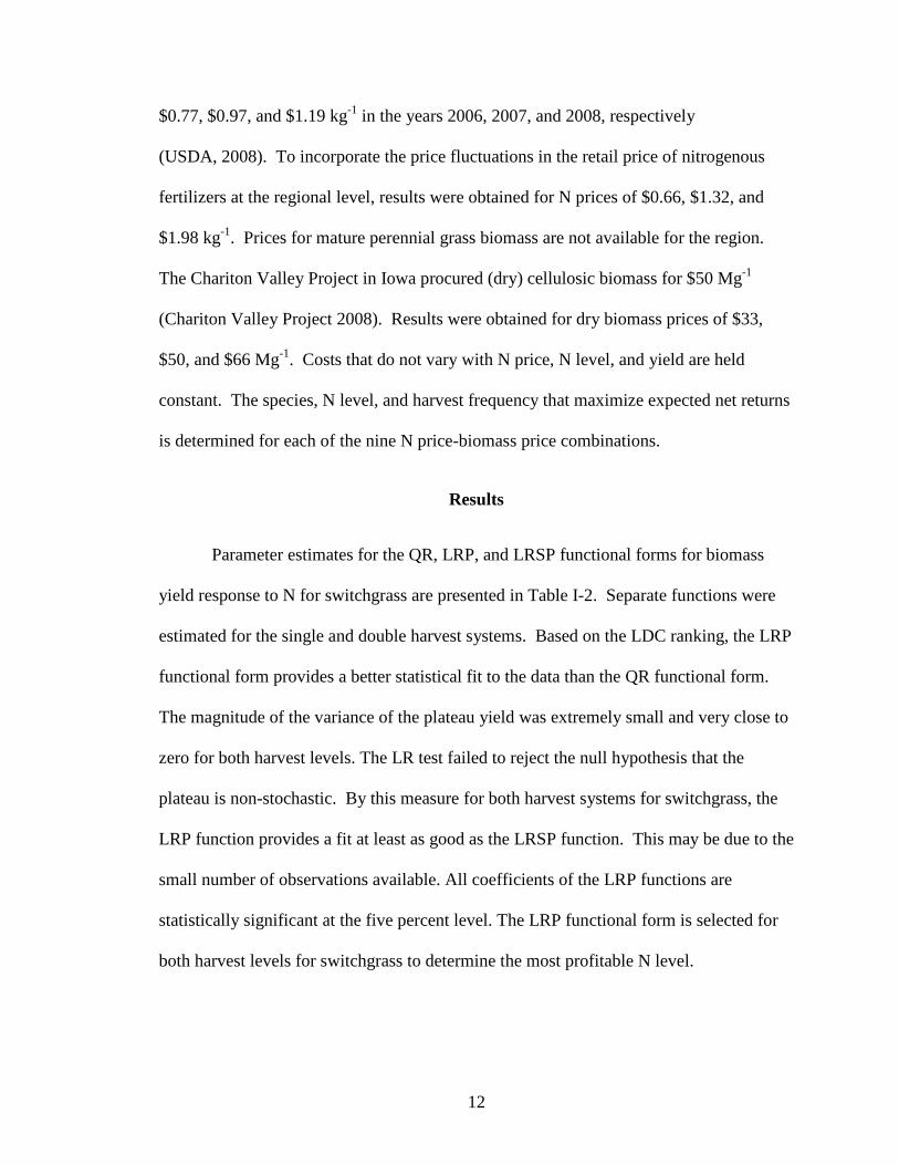
Parameter estimates for the QR, LRP, and LRSP functional forms for biomass
yield response to N for switchgrass are presented in Table I-2. Separate functions were
estimated for the single and double harvest systems. Based on the LDC ranking, the LRP
functional form provides a better statistical fit to the data than the QR functional form.
The magnitude of the variance of the plateau yield was extremely small and very close to
zero for both harvest levels. The LR test failed to reject the null hypothesis that the
plateau is non-stochastic. By this measure for both harvest systems for switchgrass, the
LRP function provides a fit at least as good as the LRSP function. This may be due to the
small number of observations available. All coefficients of the LRP functions are
statistically significant at the five percent level. The LRP functional form is selected for
both harvest levels for switchgrass to determine the most profitable N level.
13
Table I-2 Biomass yield response to nitrogen functions for switchgrass
Statistic
Single Harvest Double Harvest
Quadratic Linear
Response Plateau
Linear Response Stochastic
Plateau
Quadratic Linear
Response Plateau
Linear Response Stochastic
Plateau
Intercept 7.488** (0.853)a
5.284** (1.075)
5.284** (1.075)
6.485** (0.844)
6.462** (0.609)
6.919* (0.074)
Nitrogen (kg ha-1) 0.060* (0.016)
0.100** (0.020)
0.100 (0.202)
0.052* (0.014)
0.036** (0.006)
0.037 (0.536)
Nitrogen squared -0.00016* (0.00005) _ _ -0.00009
(0.00005) _ _
Plateau yield (Mg ha-1) _ 12.232** (0.340)
12.232** (0.340) _ 13.364**
(0.511) 13.820** (0.600)
Variance of plateau yield 0.000 _ 0.176
(0.958)
Log likelihood -58.35 -53.95 -53.95 -56.10 -55.50 -55.80
Akaike Information Criterion 126.70 117.90 119.95 122.20 121.00 123.60
Bayesian Information Criterion 122.10 113.40 114.50 117.70 116.50 118.20
Note: The dependent variable is dry matter yield in Mg ha-1 yr-1 for years after establishment. Number of observations used for the estimation of each response function is 48. * Statistically significant at the 10% level. ** Statistically significant at the 5% level. a Standard errors are in parenthesis.

14
The estimated plateau yield from the LRP function for a single harvest is 12.2 Mg
ha-1 yr-1. The spline point in the LRP single harvest function occurs at a N level of 69 kg
ha-1 yr-1. However, the expected yield based on the LRP double harvest function from 69
kg N ha-1 yr-1 is only 9.0 Mg ha-1 yr-1. Based on the LRP double harvest function, 160 kg
N ha-1 yr-1 would be required to produce 12.2 Mg ha-1 yr-1. The LRP double harvest
function has an estimated plateau yield of 13.4 Mg ha-1 yr-1 from 192 kg N ha-1 yr-1.
These results are consistent with those reported by others who recommend that N
application rates to stands of established switchgrass fall within a range from 56 to 168
kg ha-1 yr-1 (Muir et al. 2001; Vogel et al. 2002; Mulkey, Owens, and Lee 2006; Fike et
al. 2006). Switchgrass production systems that include a harvest during the active
growing period followed by a second harvest after senescence require more N. In the
region, switchgrass growth is slow to recover after a July harvest.
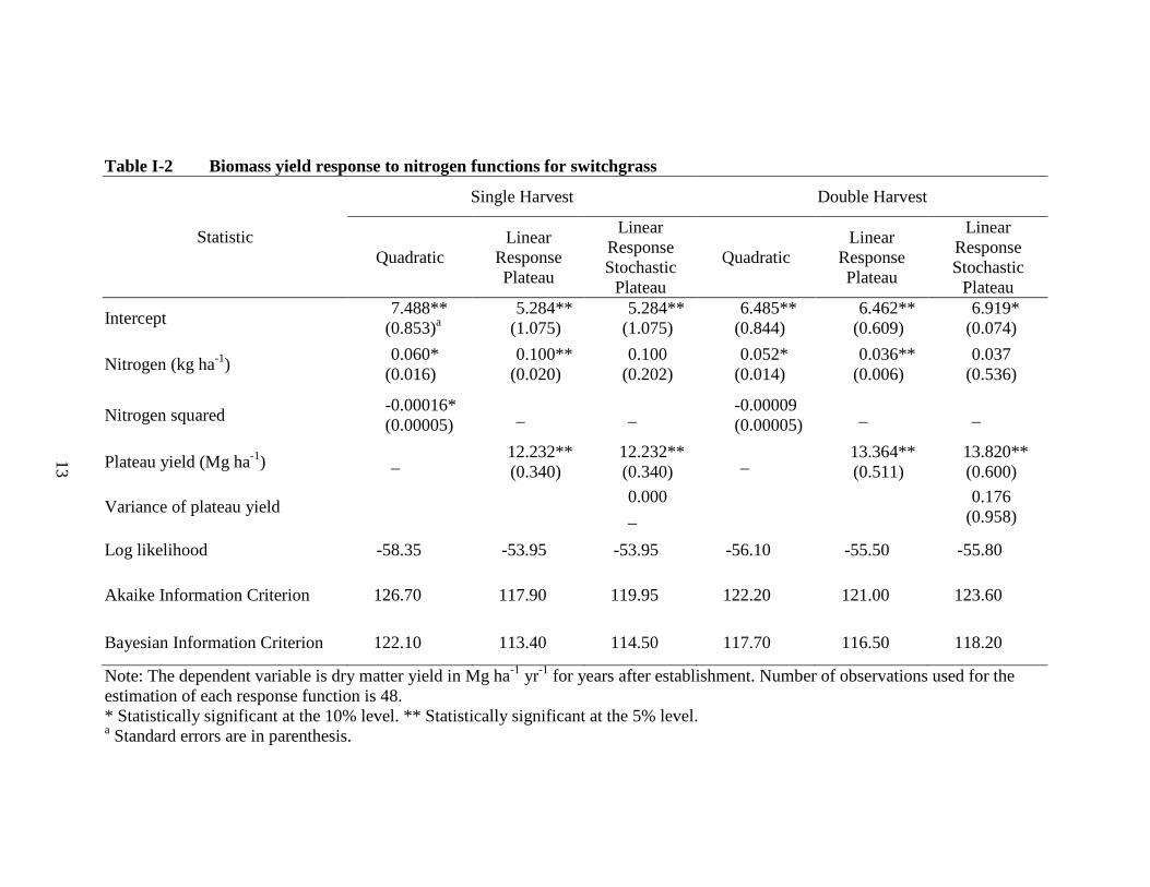
Table I-3 includes the regression results of biomass yield response for
bermudagrass. The LR test indicates that the LRSP functional form is statistically
superior to the LRP functional form for the single harvest plots. Based on the LDC
ranking, the LRSP model is also preferred over the QR model when only a single harvest
is conducted per year. For the double harvest plots, the statistical tests cannot distinguish
among the three functional forms. Since the LRSP form was selected for the single
harvest system, it was also selected for the double harvest system.
The variance identified with estimation of the LRSP plateau yield indicates that
bermudagrass biomass yield is sensitive to weather conditions that vary from year to
year. The variance associated with the plateau yield for a double harvest is
15
Table I-3 Biomass yield response to nitrogen functions for bermudagrass
Statistic
Single Harvest Double Harvest
Quadratic Linear Response Plateau
Linear Response Stochastic
Plateau Quadratic Linear Response
Plateau
Linear Response Stochastic
Plateau
Intercept 3.830** (0.768)a
4.019** (0.515)
4.117* (0.417)
5.237** (0.959)
5.873** (0.741)
5.871* (0.685)
Nitrogen (kg ha-1) 0.042* (0.010)
0.030** (0.004)
0.032* (0.040)
0.066* (0.016)
0.046** (0.008)
0.046 (0.790)
Nitrogen squared -0.00005 (0.00004) _ _ -0.00011
(0.00005) _ _
Plateau yield (Mg ha-1) _ 10.290** (0.448)
10.732** (0.780) _ 14.529**
(0.620) 14.500** (0.907)
Variance of plateau yield 4.210
(2.634) 2.052 (2.072)
Log likelihood -43.70 -44.05 -38.30 -63.25 -63.25 -62.30
Akaike Information Criterion 97.40 98.10 88.60 136.40 136.50 136.60
Bayesian Information Criterion 92.80 93.60 83.20 131.90 132.00 131.20
Note:The dependent variable is dry matter yield in Mg ha-1 yr-1 for years after establishment. Number of observations used for the estimation of each response function is 48. * Statistically significant at 10% level . ** Statistically significant at 5% level. a Standard errors are in parenthesis.

16
approximately half of that associated with a single harvest. Total biomass expected yield
is not only greater but more stable across years from the double harvest system.
For an annual application rate of 239 kg N ha-1 yr-1, the estimated bermudagrass
yield is 10.3 Mg ha-1 yr-1 for a single harvest and 14.4 Mg ha-1 yr-1 when N is applied in
two split doses and the grass is harvested twice yr-1. Harvestable bermudagrass yield
increases when harvested more than once yr-1. The plateau yield increases from 10.7 Mg
ha-1 to 14.5 Mg ha-1 yr-1 when N is applied in split doses and the biomass is harvested
twice per year. This finding is consistent with prior studies that have found that
bermudagrass has high N response, a high after-harvest growth rate and a fast recovery
from a July cutting (Overman, Scholtz, and Taliaferro 2003; Scarbrough et al. 2004;
Silveria, Haby, and Leonard 2007; USDA-NRCS 2008;).
Response function parameter estimates for lovegrass are reported in Table I-4.
Based on the LR test, the LRP functional form is statistically superior to the LRSP form
for both harvest systems. The plateau variance for the LRSP was close to zero. Based on
the LDC ranking, the LRP model also fits the data better than the QR functional form.
The LRP functional form is selected to represent lovegrass biomass yield response to N
for both harvest levels. All parameter estimates for the LRP functions are statistically
significant at the five percent level. Based on the LRP functional form, the single
(double) harvest lovegrass plateau yield of 8.5 (12.3) Mg ha-1 yr-1 is achieved with an
annual application of 78 (149) kg N. This finding is consistent with that reported
elsewhere (McMurphy, Denman, and Tucker 1975; Taliaferro et al. 1975; Edwards
2000). Parameter estimates for flaccidgrass response functions are reported in Table I-5.

17
Table I-4 Biomass yield response to nitrogen functions for lovegrass
Statistic
Single Harvest Double Harvest
Quadratic Linear
Response Plateau
Linear Response Stochastic
Plateau
Quadratic Linear Response Plateau
Linear Response Stochastic
Plateau
Intercept 4.713** (0.618)a
4.012** (0.623)
3.985 (0.641)
3.535** (0.726)
4.583** (0.549)
4.563* (0.540)
Nitrogen (kg ha-1) 0.046* (0.012)
0.058** (0.012)
0.060 (0.130)
0.086** (0.012)
0.052** (0.006)
0.053* (0.062)
Nitrogen squared -0.00011 (0.00004) -- -0.00018**
(0.00004) --
Plateau yield (Mg ha-1) 8.530** (0.502)
8.525* (0.533) -- 12.346**
(0.452) 12.354** (0.526)
Variance of plateau yield 0.186 (0.506) 0.346
(0.622)
Log likelihood -49.25 -46.85 -46.80 -50.40 -50.00 -49.80
Akaike Information Criterion 110.50 105.70 107.60 110.80 110.00 111.60
Bayesian Information Criterion 105.10 100.30 101.20 106.30 105.50 106.20
Note:The dependent variable is dry matter yield in Mg ha-1 yr-1 for years after establishment. Number of observations used for the estimation of each response function is 48. * Statistically significant at 10% level. ** Statistically significant at 5% level. a Standard errors are in parenthesis.
18
Table I-5 Biomass yield response to nitrogen functions for flaccidgrass
Statistic
Single Harvest Double Harvest
Quadratic
Linear Response Plateau
Linear Response Stochastic
Plateau Quadratic
Linear Response Plateau
Linear Response Stochastic
Plateau
Intercept 8.516** (0.786)a
8.756** (0.598)
4.655*** (0.047)
6.070** (0.818)
6.673** (0.609)
6.675* (0.609)
Nitrogen (kg ha-1) 0.010 (0.014)
0.004 (0.006)
0.110* (0.123)
0.064** (0.014)
0.044** (0.006)
0.044* (0.686)
Nitrogen squared -0.00002 (0.00005) -- -- -0.00013
(0.00005) --
Plateau yield (Mg ha-1) -- 9.717** (0.488)
9.528** (0.392) 13.991**
(0.497) 13.988** (0.497)
Variance of plateau yield 0.246 (0.386) 0.000
_
Log likelihood -54.50 -54.60 -52.80 -56.35 -55.55 -55.55
Akaike Information Criterion 123.10 119.20 117.60 122.70 121.10 123.10
Bayesian Information Criterion 117.70 114.70 112.20 118.20 116.60 117.70 Note: The dependent variable is dry matter yield in Mg ha-1 yr-1 for years after establishment. Number of observations used for the estimation of each response function is 48. *Statistically significant at 10% level. ** Statistically significant at 5% level. a Standard errors are in parenthesis.
19
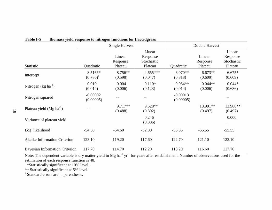
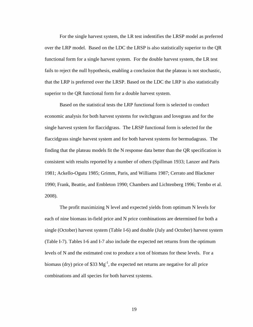
For the single harvest system, the LR test indentifies the LRSP model as preferred
over the LRP model. Based on the LDC the LRSP is also statistically superior to the QR
functional form for a single harvest system. For the double harvest system, the LR test
fails to reject the null hypothesis, enabling a conclusion that the plateau is not stochastic,
that the LRP is preferred over the LRSP. Based on the LDC the LRP is also statistically
superior to the QR functional form for a double harvest system.
Based on the statistical tests the LRP functional form is selected to conduct
economic analysis for both harvest systems for switchgrass and lovegrass and for the
single harvest system for flaccidgrass. The LRSP functional form is selected for the
flaccidgrass single harvest system and for both harvest systems for bermudagrass. The
finding that the plateau models fit the N response data better than the QR specification is
consistent with results reported by a number of others (Spillman 1933; Lanzer and Paris
1981; Ackello-Ogutu 1985; Grimm, Paris, and Williams 1987; Cerrato and Blackmer
1990; Frank, Beattie, and Embleton 1990; Chambers and Lichtenberg 1996; Tembo et al.
2008).
The profit maximizing N level and expected yields from optimum N levels for
each of nine biomass in-field price and N price combinations are determined for both a
single (October) harvest system (Table I-6) and double (July and October) harvest system
(Table I-7). Tables I-6 and I-7 also include the expected net returns from the optimum
levels of N and the estimated cost to produce a ton of biomass for these levels. For a
biomass (dry) price of $33 Mg-1, the expected net returns are negative for all price
combinations and all species for both harvest systems.
20
Table I-6 Estimates of profit maximizing nitrogen level, expected yield, cost and expected net returns for the selected grass species when harvested once per year in October.
In-Field Price of Biomass ($ Mg-1)
Price of Nitrogen ($ kg-1)
Switchgrass Bermudagrass Lovegrass Flaccidgrass
0.66 1.32 1.98 0.66 1.32 1.98 0.66 1.32 1.98 0.66 1.32 1.98
Profit maximizing N level (kg N ha-1 yr-1)a
33 69 69 69 186 0 0 78 78 0 48 46 44
50 69 69 69 221 144 0 78 78 78 49 47 46
66 69 69 69 239 186 109 78 78 78 50 48 47
Profit maximizing expected yield (Mg ha-1 yr-1)a
33 12.2 12.2 12.2 9.5 4.1 4.1 8.5 8.5 4.0 9.0 8.8 8.6
50 12.2 12.2 12.2 10.0 8.5 4.1 8.5 8.5 8.5 9.1 8.9 8.8
66 12.2 12.2 12.2 10.3 9.5 7.5 8.5 8.5 8.5 9.2 9.0 8.9
Profit maximizing cost of production ($ Mg -1) b
33 39 43 46 56 74 74 47 54 65 50 54 57
50 39 43 46 56 69 74 47 54 61 50 54 57
66 39 43 46 57 69 79 47 54 61 49 53 57
Profit maximizing expected net returns ($ ha-1 yr-1)
33 -69 -116 -163 -222 -165 -165 -123 -178 -131 -148 -183 -212
50 133 86 40 -69 -165 -99 17 -37 -91 2 -35 -69
66 336 289 242 94 -37 -99 158 104 49 158 116 79 a Based on LR test and LDC the suitable response functions were LRP for switchgrass
and lovegrass and LSRP for bermudagrass, and flaccidgrass. These response functions are used for the estimation of optimum N and optimum yield.
b Costs are not included for collecting bales and transporting bales from the field. Charges were not assessed for overhead, risk, and management.

21
For a biomass price of $50 Mg-1, and N prices of $1.32 and $1.98 per kg-1,
expected net returns are negative for bermudagrass, lovegrass, and flaccidgrass for both
harvest systems. For an in-field biomass price of $50 Mg-1, expected net returns are
positive for the single harvest switchgrass system for all three N prices. For an in-field
biomass price of $66 Mg-1, expected net returns are positive for all species, all N price
levels and both harvest systems, except for the single harvest bermudagrass systems with
N prices of $1.32 and $1.98 kg-1.
For a single harvest system, the expected net returns for switchgrass are greater
than the expected net returns for bermudagrass and flaccidgrass for each of the nine
biomass price and N price combinations. For eight of the nine price combinations,
expected net returns are also greater for switchgrass than for lovegrass. However, for a
biomass price of $33 Mg-1 and N price of $1.98 kg-1 , the expected net returns are -$163
ha-1 for switchgrass and -$131 ha-1 for lovegrass. These estimates follow from the
assumption that biomass harvest is required. In low biomass price situations, if the value
of the biomass is less than harvest cost, it would be optimal to not harvest.
In general, with a single harvest system, bermudagrass has the highest N
requirement and the highest cost per ton of biomass followed by lovegrass. In most
cases, bermudagrass records the lowest expected net returns among the four grass
species. Switchgrass records the highest expected yield, lowest cost per ton, and highest
expected net return per hectare. A comparison across harvest systems indicates that for
most of the species, the double harvest system more than doubles the optimum N
application.
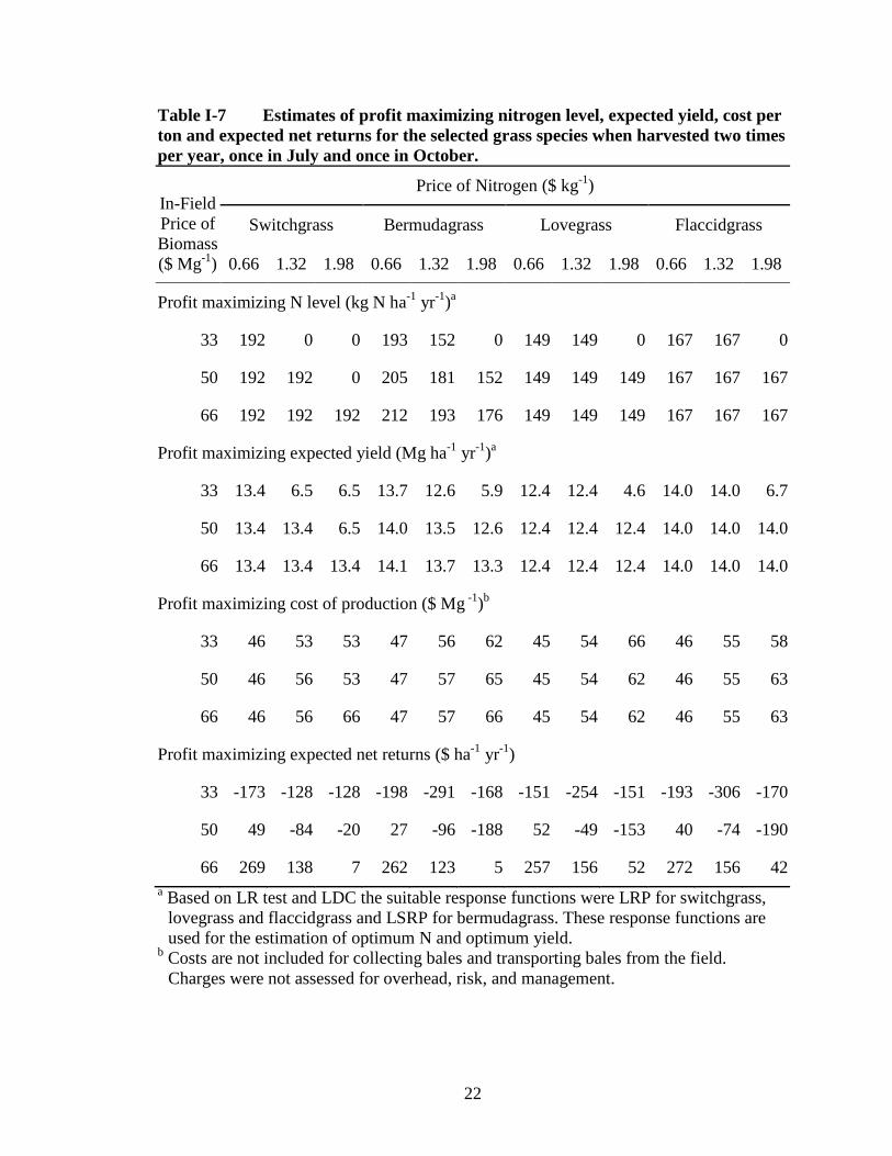
22
Table I-7 Estimates of profit maximizing nitrogen level, expected yield, cost per ton and expected net returns for the selected grass species when harvested two times per year, once in July and once in October.
In-Field Price of Biomass ($ Mg-1)
Price of Nitrogen ($ kg-1)
Switchgrass Bermudagrass Lovegrass Flaccidgrass
0.66 1.32 1.98 0.66 1.32 1.98 0.66 1.32 1.98 0.66 1.32 1.98
Profit maximizing N level (kg N ha-1 yr-1)a
33 192 0 0 193 152 0 149 149 0 167 167 0
50 192 192 0 205 181 152 149 149 149 167 167 167
66 192 192 192 212 193 176 149 149 149 167 167 167
Profit maximizing expected yield (Mg ha-1 yr-1)a
33 13.4 6.5 6.5 13.7 12.6 5.9 12.4 12.4 4.6 14.0 14.0 6.7
50 13.4 13.4 6.5 14.0 13.5 12.6 12.4 12.4 12.4 14.0 14.0 14.0
66 13.4 13.4 13.4 14.1 13.7 13.3 12.4 12.4 12.4 14.0 14.0 14.0
Profit maximizing cost of production ($ Mg -1)b
33 46 53 53 47 56 62 45 54 66 46 55 58
50 46 56 53 47 57 65 45 54 62 46 55 63
66 46 56 66 47 57 66 45 54 62 46 55 63
Profit maximizing expected net returns ($ ha-1 yr-1)
33 -173 -128 -128 -198 -291 -168 -151 -254 -151 -193 -306 -170
50 49 -84 -20 27 -96 -188 52 -49 -153 40 -74 -190
66 269 138 7 262 123 5 257 156 52 272 156 42 a Based on LR test and LDC the suitable response functions were LRP for switchgrass,
lovegrass and flaccidgrass and LSRP for bermudagrass. These response functions are used for the estimation of optimum N and optimum yield.
b Costs are not included for collecting bales and transporting bales from the field. Charges were not assessed for overhead, risk, and management.
23
For the high biomass price and low N price combinations, the increment in the
yield covers the additional expenses for fertilizer, application costs, and harvesting for
bermudagrass, lovegrass, and flaccidgrass. This fact is evident from the reduction in cost
of biomass for these species for some of the price combinations. On the other hand, for
switchgrass, the cost of biomass produced is greater for the double harvest system for all
price combinations. For the highest budgeted in-field biomass price of $66 Mg-1, the
double harvest system is more profitable for all grasses except switchgrass.
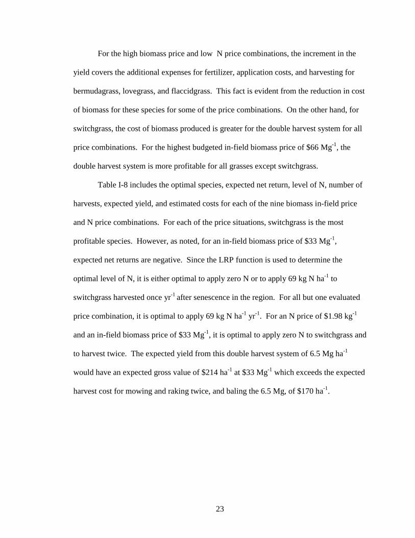
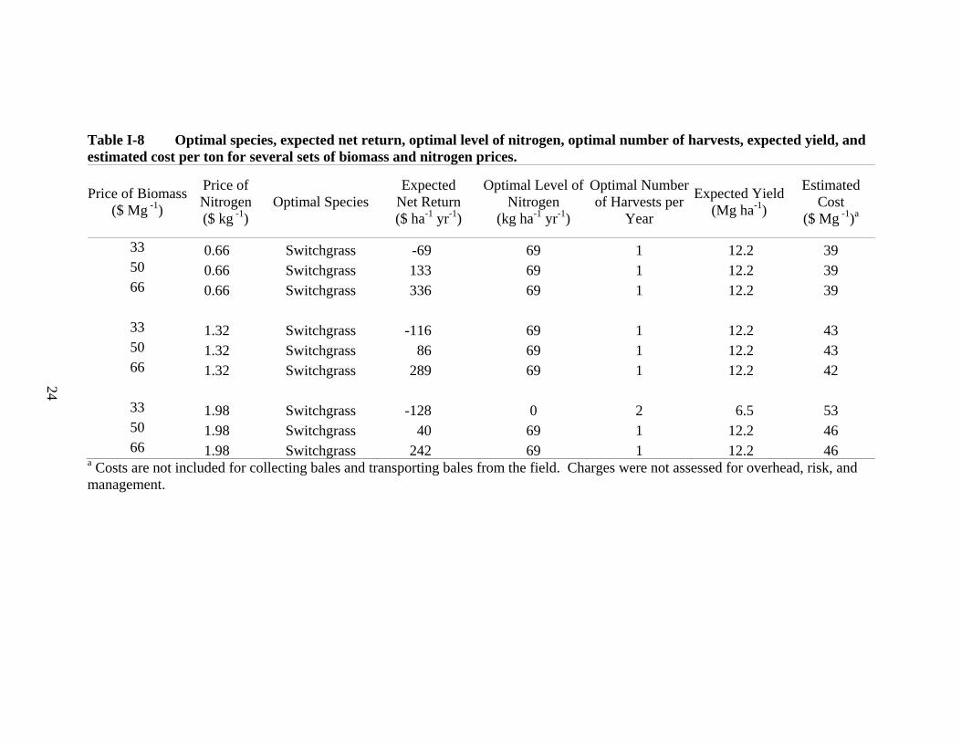
Table I-8 includes the optimal species, expected net return, level of N, number of
harvests, expected yield, and estimated costs for each of the nine biomass in-field price
and N price combinations. For each of the price situations, switchgrass is the most
profitable species. However, as noted, for an in-field biomass price of $33 Mg-1,
expected net returns are negative. Since the LRP function is used to determine the
optimal level of N, it is either optimal to apply zero N or to apply 69 kg N ha-1 to
switchgrass harvested once yr-1 after senescence in the region. For all but one evaluated
price combination, it is optimal to apply 69 kg N ha-1 yr-1. For an N price of $1.98 kg-1
and an in-field biomass price of $33 Mg-1, it is optimal to apply zero N to switchgrass and
to harvest twice. The expected yield from this double harvest system of 6.5 Mg ha-1
would have an expected gross value of $214 ha-1 at $33 Mg-1 which exceeds the expected
harvest cost for mowing and raking twice, and baling the 6.5 Mg, of $170 ha-1.
24
Table I-8 Optimal species, expected net return, optimal level of nitrogen, optimal number of harvests, expected yield, and estimated cost per ton for several sets of biomass and nitrogen prices.
Price of Biomass ($ Mg -1)
Price of Nitrogen ($ kg -1)
Optimal Species Expected
Net Return ($ ha-1 yr-1)
Optimal Level of Nitrogen
(kg ha-1 yr-1)
Optimal Number of Harvests per
Year
Expected Yield(Mg ha-1)
Estimated Cost
($ Mg -1)a
33 0.66 Switchgrass -69 69 1 12.2 39 50 0.66 Switchgrass 133 69 1 12.2 39 66 0.66 Switchgrass 336 69 1 12.2 39
33 1.32 Switchgrass -116 69 1 12.2 43 50 1.32 Switchgrass 86 69 1 12.2 43 66 1.32 Switchgrass 289 69 1 12.2 42
33 1.98 Switchgrass -128 0 2 6.5 53 50 1.98 Switchgrass 40 69 1 12.2 46 66 1.98 Switchgrass 242 69 1 12.2 46
a Costs are not included for collecting bales and transporting bales from the field. Charges were not assessed for overhead, risk, and management.
25
Conclusion and Discussion
Biomass yield to N response functions were estimated for four perennial grass
species and to determine the species. These functions were used to estimate the species,
N level, and harvest frequency that will maximize expected net returns to a land unit,
given the climate and soils of the U.S.A. Southern Plains. For each of the four species
and both harvest systems, the functional forms that include a plateau, either the LRP or
LRSP, fits the data better than the QR functional form that forces a unique maximum and
forces symmetry relative to the maximum point. This finding is consistent with results
reported by a number of researchers.
For in-field biomass prices ranging from $33 to $66 Mg-1 and N prices ranging
from $0.66 to $1.98 kg-1, switchgrass is the optimal species. For a biomass price of $50
Mg-1 it is optimal to fertilize switchgrass with 69 kg ha-1 in the spring and to harvest once
yr-1 after senescence in October. For an N price of $1.32 kg-1, expected net returns are
$133, $86, and $40 ha-1 yr-1 for in-field biomass prices of $50 Mg-1. For N prices of
$0.66, $1.32, and $1.98 kg-1, breakeven in-field prices for the optimal switchgrass
production systems are $39, $43, and $53 Mg-1, respectively.
Nitrogen treatment levels in the designed experiment were 34, 67, 134, and 269
kg ha-1 yr-1. The estimated yield plateau for switchgrass harvested once is 69 kg ha-1 yr-1.
Thus, two of the points are on the slope and two are on the plateau of the LRP function
and are theoretically sufficient to provide relatively precise response function parameter
estimates. Field trials are costly to execute and adding N levels would add to the cost of
the trials. However, if too few treatment levels are included in the field trials, resulting in
parameter estimates with large standard deviation, recommendations from estimated

26
response functions could also be costly. For the region of the study, switchgrass would
be a more economical species for biomass feedstock production than either
bermudagrass, or lovegrass, or flaccidgrass. However, the assumption that each of the
four species would be of equal value to a cellulosic biorefinery remains to be confirmed.
Prior research has found that switchgrass does not respond to potassium and phosphorus
fertilization and that if harvest of a perennial grass is delayed until after senescence,
removal of above ground parts of the plant will not mine phosphorus and potassium from
the soil. However, one shortcoming of the field trials was that soil tests were not
conducted after the study to confirm that levels of phosphorus and potassium in the soil
had not been depleted.
27
PAPER I REFERENCES
Ackello-Ogutu, C., Q. Paris, and W.A. Williams. 1985. “Testing A a Von Liebig Crop Response Function Against Polynomial Specifications.” American Journal of Agricultural Economics 64:873-880.
Aden, A., M. Ruth, K. Ibsen, J. Jechura, K. Neeves, J. Sheehan, B. Wallace, L. Montague, A. Slayton, and J. Lukas. 2002. “Lignocellulosic Biomass to Ethanol Process Design and Economics Utilizing Co-Current Dilute Acid Prehydrolysis and Enzymatic Hydrolysis for Corn Stover.” Report NREL/TP-510-32438, Golden CO, National Renewable Energy Laboratory.
Belesky, D.P., J.C. Burns, D.S. Chamblee, D.W. Daniel, J.M. de Ruiter, D.S. Fisher, J.T. Green, R.D. Mochrie, J.P.Mueller, K.R. Pond, and D.H. Timothy. 1998. Carostan Flaccidgrass: Establishment, Adaptation, Production Management, Forages Quality, and Utilization. North Carolina State University, Technical Bulletin 313.
Boateng, A.A., W.F. Anderson, and G.J. Phillips. 2007. “Bermudagrass for Biofuels: Effect of Two Genotypes on Pyrolysis Product Yield.” Energy and Fuels 21:1183-1187.
Burns, J.C., D.S. Chamblee, D.P. Belesky, D.S. Fisher, and D.H. Timothy. 1998. “Nitrogen and Defoliation Management: Effects on Yield and Nutritive Value of Flaccidgrass.” Agronomy Journal 90:85–92.
Caputo, A.C., M. Palumbo, P.M. Pelagagge, and F. Scacchia. 2005. “Economics of Biomass Energy Utilization in Combustion and Gasification Plants: Effects of Logistic Variables.” Biomass and Bioenergy 28:35-51.
Cerrato, M.E., and A.M. Blackmer. 1990. “Comparison of Models for Describing Corn Yield Response To to Nitrogen Fertilizer.” Agronomy Journal 82:138–143.
Chambers, R.G. and Lichtenberg E. A. 1996. “Nonparametric Approach to the Von Liebig-Paris Technology.” American Journal of Agricultural Economics 78:373–86.
Chariton Valley Project. 2008. Economic Benefits. Ottumwa, IA: Available from: <http://www.iowaswitchgrass.com> , [Accessed May 2008].

28
Doye, D., R. Sahs, and D.Kletke. 2005. Oklahoma Farm and Range Custom Rates, 2005-2006. CR-205, Stillwater, OK: Oklahoma State University Cooperative Extension Service.
Edwards, S. 2000. Weeping Lovegrass as a Potential Bioenergy Crop. Jamie L. Whitten Plant Materials Center Technical Report vol. 15, no. 7, Coffeeville, MS.
Evanylo, G.K. 1991. “No-Till Corn Response to Nitrogen Rate and Timing in the Middle of Atlantic Coastal Plain.” Journal of Production Agriculture 4:180-185.
Fike, J.H., D.J. Parrish, D.D. Wolf, J.A. Balasko, J.T. Green Jr, Rasnake M, and J.H. Reynolds. 2006. “Switchgrass Production for the Upper Southeastern USA: Influence of Cultivar and Cutting Frequency on Biomass Yields.” Biomass and Bioenergy 30:207-213.
Frank, M.D., B.R. Beattie, and M.E. Embleton. 1990. “A Comparison of Alternative Crop Response Models.” American Journal of Agricultural Economics 72:597-603.
Fuentes, R.G., and C.M.Taliaferro. “Biomass Yield Stability of Switchgrass Cultivars.” Trends in New Crops and New Uses. J. Janick, and A. Whipkey, eds., pp.276-282. Alexandria VA: ASHS Press, 2002.
Greene, W. Econometric Analysis, 5th ed. Upper Saddle River: Prentice Hall. 2003.
Grimm, S.S., Q. Paris, and W.A. Williams. 1987. “A Von Liebig Model for Water and Nitrogen Crop Response.” Western Journal of Agricultural Economics 12:182-192.
Jung, G.A., J.A. Shaffer, and W.L. Stout. 1998. “Switchgrass and Big Bluestem Responses to Amendments on Strongly Acid Soil.” Agronomy Journal 80:669–676.
Kaitibie, S., W.E. Nganje, B.W. Brorsen and F.M. Epplin 2007. “A Cox Parametric Bootstrap Test of the von Liebig Hypotheses.” Canadian Journal of Agricultural Economics 55:15–25.
Klasson, K.T., B.B. Elmore, J.L. Vega, M.D. Ackerson, E.C. Clausen, and J.L. Gaddy.
1990. “Biological Production of Liquid and Gaseous Fuels from Synthesis Gas.” Applied Biochemistry and Bioengineering 25:857-873.
Lanzer, E.A., and Q.Paris. 1981. “A New Analytical Framework for the Fertilization Problem.” American Journal of Agricultural Economics 63:93–103.
Lee, D.K., and A. Boe. 2005. “Biomass Production of Switchgrass in Central South Dakota.” Crop Science 45:2583-2590.

29
Lee, D.K., V.N. Owens, and J.J. Doolittle. 2007. “Switchgrass and Soil Carbon Sequestration Response to Ammonium Nitrate, Manure, and Harvest Frequency on Conservation Reserve Program Land.” Agronomy Journal 99:462-468.
Lewandowski, I., J.M.O. Scurlock, E. Lindvall, and M. Christou. 2003. “The Development and Current Status of Perennial Rhizomatous Grasses as Energy Crops in the US and Europe.” Biomass and Bioenergy 25:335-361.
Littell, R.C., G.A. Milliken, W.W. Stroup, and R.D. Wolfinger. SAS Systems for Mixed Models. Cary NC: SAS Institute Inc., 2002.
Llewelyn, R.V., and A.M. Featherstone. 1997. “A Comparison of Crop Production Functions Using Simulated Data for Irrigated Corn in Western Kansas.” Agricultural Systems 54:521-538.
McKendry, P. 2002. “Energy Production From Biomass (Part 2): Conversion Technologies.” Bioresource Technology 83:47-54.
McLaughlin, S., J. Bouton, D. Bransby, B. Conger, W. Ocumpaugh, D. Parrish, C. Taliaferro, K. Vogel, and S. Wullschleger. “Developing Switchgrass as a Bioenergy Crop.” Perspectives on New Crops and New Uses. J. Janick, ed., pp. 282-299. Alexandria VA: ASHS Press, 1999.
McLaughlin, S.B., and L.A. Kszos. 2005. “Development of Switchgrass (Panicum virgatum) as a Bioenergy Feedstock in the United States.” Biomass and Bioenergy 28:515-535.
McMurphy, W.E., C.E. Denman, and B.B. Tucker. 1975. “Fertilization of Native Grass and Weeping Lovegrass.” Agronomy Journal 67:233-236.
Mjelde, J.W., J.T. Cothern, M.E. Rister, F.M. Hons, C. Coffman, and G.C.R. Shumway. 1991. “Integrating Data From from Various Field Experiments: the The Case of Corn in Texas.” Journal of Production Agriculture 4:139-147.
Mosier, N., C. Wyman, B. Dale, R. Elander, Y.Y. Lee, M. Holtzapple, and M. Ladisch. 2005. “Features of Promising Technologies for Pretreatment of Lignocellulosic Biomass.” Bioresource Technology 96:673-686.
Muir, J.P., M.A. Sanderson, W.R. Ocumpaugh, R.M. Jones, and R.L. Reed. 2001. “Biomass Production of ‘Alamo’ Switchgrass in Response to Nitrogen, Phosphorus, and Row Spacing.” Agronomy Journal 93:896–901.
Mulkey, V.R., V.N. Owens, and D.K. Lee. 2006. “Management of Switchgrass-Dominated Conservation Reserve Program Lands for Biomass Production in South Dakota.” Crop Science 46:712-720.

30
Overman, A.R., R.V. Scholtz, and C.M. Taliaferro. 2003. “Model Analysis of Response of Bermudagrass to Applied Nitrogen.” Communications in Soil Science and Plant Analysis 34(9&10):1303–1310.
Paris, Q. 1992. “The Von Liebig Hypothesis.” American Journal of Agricultural Economics” 74:1019–1028.
Parrish, D.J., and J.H. Fike. 2005. “The Biology and Agronomy of Switchgrass for Biofuels.” Critical Reviews in Plant Sciences 24(5):423-459.
Perlack, R.D., L.L. Wright, A.F.Turhollow, R.L. Graham, B.J. Stokes, and D.C. Erbach. 2005. Biomass as Feedstock for a Bioenergy and Bioproducts Industry: the Technical Feasibility of a Billion-Ton Annual Supply. Oak Ridge TN: U.S. Department of Energy.
Perrin. R.K. 1976. “The Value of Information and the Value of Theoretical Models in Crop Response Research.” American Journal of Agricultural Economics 58:54-61.
Pinheiro, J.C., and D.M. Bates. 2005. "Approximations to the Log-Likelihood Function in the Nonlinear Mixed-Effects Model." Journal of Computational and Graphical Statistics 4(1):12-35.
Pollak, R.A., and R.J. Wales. 1991. “Likelihood Dominance Criterion.” Journal of Econometrics 47:227-242.
Rajagopalan, S., R.P. Datar, and R.S. Lewis. 2002. “Formation of Ethanol from Carbon Monoxide Via a New Microbial Catalyst.” Biomass and Bioenergy 23:487-493.
Reynolds, J.H., C.L. Walker, and M.J. Kirchner. 2000. “Nitrogen Removal in Switchgrass Biomass under Two Harvest Systems.” Biomass and Bioenergy 19:281-286.
Roberts, D.C., B. W. Brorsen, W. R. Raun, and J. B. Solie. “The Value of Regional Annual Nitrogen Needs Information for Wheat Producers in Oklahoma.” Paper presented at the SAEA annual meetings, Dallas, TX, 2 – 6 February 2008.
Rogers, J. 2006. Evaluation of Warm-Season Perennial Grasses. Rep. NF-FO-06-02.
Ardmore OK: The Samuel Roberts Noble Foundation. Available at: http://www.noble.org/ag/Forage/06WarmSeasonGrasses/index.html [Accessed Dec. 2008; verified Sept. 2009].
Sanderson, M.A., P.R. Adler, A.A. Boateng, M.D. Casler, and G. Sarath. 2006. “Switchgrass as a Biofuels Feedstock in the USA.” Canadian Journal of Plant Science 86:1315-25.
SAS Institute. The NLMIXED Procedure. Cary, North Carolina: SAS Institute Inc., 2004. Availiable at http://v8doc.sas.com/sashtml/.

31
Scarbrough, D.A., W.K. Coblentz, K.P. Coffey, K.F. Harrison, T.F. Smith, D.S. Hubbell III, J.B. Humphry, Z.B. Johnson, and J. E.Turner. 2004. “Effects of Nitrogen Fertilization Rate, Stockpiling Initiation Date, and Harvest Date on Canopy Height and Dry Matter Yield of Autumn-Stockpiled Bermudagrass.” Agronomy Journal 96:538–546.
Schlegel, A.J., and J.L. Halvin. 1995. “Corn Response to Long-Term Nitrogen and Phosphorous Fertilization.” Journal of Production of Agriculture 8:181-185.
Service, R.F. 2007. “Cellulosic Ethanol: Biofuel Researchers Prepare to to Reap A a New Harvest.” Science 315:1488-1491.
Silveria, M.L., V.A. Haby, and L. Leonard. 2007. “ Response of Costal Bermudagrass Yield and Nutrient Uptake Efficiency to Nitrogen Sources.” Agronomy Journal 99:707-714.
Spillman, W.J. 1933. “Use of the Exponential Yield Curve in Fertilizer Experiments.” Technical Bulletin No. 348, Washington, DC: United States Department of Agriculture.
Taliaferro, C.M., F.P. Horn, B.B. Tucker, R. Totusek, and R.D. Morrison. 1975. “Performance of Three Warm-Season Perennial Grasses and a Native Range Mixture as Influenced by N and P Fertilization.” Agronomy Journal 67:289-292.
Tembo, G., B. W.Brorsen, F.M. Epplin, and E.Tostão. 2008. “Crop Input Response Functions With with Stochastic Plateaus.” American Journal of Agricultural Economics 90:424-434.
Thomason, W.E., W.R. Raun, G.V. Johnson, C.M. Taliaferro, K.W. Freeman, and K.J. Wynn. 2004. “Switchgrass Response to Harvest Frequency and Time and Rate of Applied Nitrogen.” Journal of Plant Nutrition 27:1199-1226.
U.S. Department of Agriculture (USDA). 2008. U.S. Fertilizer Imports/Exports: Summary of the Data Findings. Washington, DC: Economic Research Service. Available from: <http://www.ers.usda.gov/Data/FertilizerTrade/summary.htm.> [Accessed December 20, 2008].
U.S. Department of Agriculture (USDA/NRCS). 2008. The PLANTS Database, Panicum virgatum L. Switchgrass. Baton Rouge, LA: National Plant Data Center, Available from <http://www.plants.usda.gov/java/profile?symbol=PAVI2>. [Accessed December 20, 2008].
Vanotti, M.B., and L.G. Bundy. 1994. “An Alternative Rationale for Corn Nitrogen Fertilizer Recommendations.” Journal of Production Agriculture 7:243-249.
Vogel, K.P., J.J. Brejda, D.T. Walters, and D.R. Buxton. 2002. “Switchgrass Biomass Production in the Midwest USA: Harvest and Nitrogen Management.” Agronomy Journal 94:413–420.

32
Wolfinger, R.D. Fitting Nonlinear Mixed Models with the New NLMIXED Procedure. SUGI Proceedings, Cary, North Carolina: SAS Institute Inc. 1999.
Wright, L. 2007. Historical Perspective on How and Why Switchgrass Was Selected as a “Model” High-Potential Energy Crop. Report ORNL/TM-2007/109, Oak ridge, TN: Oak Ridge National Laboratory.
Wyman, C.E. 1994. “Ethanol from Lignocellulosic Biomass: Technology, Economics, and Opportunities.” Bioresource Technology 50:3-15.
33
Chapter II
PAPER II
ECONOMICS OF SWITCHGRASS AND MISCANTHUS RELATIVE
TO COAL AS FEEDSTOCK FOR GENERATING
ELECTRICITY
Abstract
Switchgrass (Panicum virgatum) serves as a model dedicated energy crop in the
U.S.A. Miscanthus (Miscanthus x giganteus) has served a similar role in Europe. This
study was conducted to determine the most economical species, harvest frequency, and
carbon tax required for either of the two candidate feedstocks to be an economically
viable alternative for cofiring with coal for electricity generation. Biomass yield and
energy content data were obtained from a field experiment conducted near Stillwater,
Oklahoma, U.S.A., in which both grasses were established in 2002. Plots were split to
enable two harvest treatments (once and twice yr-1). The switchgrass variety ‘Alamo’,
with a single annual post senescence harvest, produced more biomass (15.87 Mg ha-1 yr-1)
than miscanthus (12.39 Mg ha-1 yr-1) and more energy (249.6 million kJ ha-1 yr-1 versus
199.7 million kJ ha-1 yr-1 for miscanthus). For the average yields obtained, the estimated
cost to produce and deliver biomass an average distance of 50 km was $43.9 Mg-1 for
switchgrass and $51.7 Mg-1 for miscanthus. Given a delivered coal price of $39.76 Mg-1
and average energy content, a carbon tax of $7 Mg-1 CO2 would be required for

34
switchgrass to be economically competitive. For the location and the environmental
conditions that prevailed during the experiment, switchgrass with one harvest per year
produced greater yields at a lower cost than miscanthus. In the absence of government
intervention such as requiring biomass use or instituting a carbon tax, biomass is not an
economically competitive feedstock for electricity generation in the region studied.
Introduction
A major portion of electricity in the U.S.A. is produced by burning coal and
natural gas. Coal is the primary fuel used by the nation’s electric power industry. It
produces 36 % of the CO2 emissions from energy use (DOE/EIA 2007; DOE 2009).
Cofiring cellulosic biomass with coal in traditional utility boilers enables substituting
fossil fuel with renewable energy sources to produce electricity and if properly executed,
reducing carbon emissions. Cofiring with cellulosic biomass requires only minor
modifications in the boilers and minimal investment in existing plants (Fraas and
Johansson 2009). Switchgrass has been cofired with coal at the Ottumwa Generating
Station near Ottumwa, Iowa, U.S.A. Technical results were promising with no slagging.
However, it was determined that in the absence of subsidies, mandates, or carbon taxes,
cofiring was not economically competitive (Olsen 2001).
Dedicated perennial grasses could be developed, which would be locally
available, dependable, and scalable substitutes for coal. According to Perlack 22 million
ha of U.S.A. land could be converted for biomass production with minimal effects on
food, feed, and fiber production (Perlack, et al. 2005). A key to ensuring a long-term
supply of biomass feedstock to a given power plant is selecting the most suitable
perennial grass species for local soil and weather conditions.
35
Several studies have been conducted to screen species to identify relative
suitability for biomass production. In the U.S.A., the Oak Ridge National Laboratory’s
(ORNL) Herbaceous Energy Crops Research Program and the Department of Energy’s
(DOE) Biofuel Development Program were some of the early efforts of integrated and
multilocational research projects designed to select suitable species (Lewandowski et al.
2003). Most of the grass species included in these studies were chosen from the pool of
native prairie grasses found on the plains of North America. The ORNL selected
switchgrass from a screening trial that included 34 species conducted on 31 different sites
spread over seven states in the United States (McLaughlin, and Walsh 1998; Wright
2007).
During this time period, miscanthus (Miscanthus x giganteus), a non-native
ornamental plant, caught the attention of researchers in Europe. Several projects were
conducted across Europe to develop and evaluate miscanthus hybrids (Lewandowski,
Scurlock, Lindvall, and Christou 2003). Miscanthus is not native to the U.S.A. and was
not included in the ORNL trials. Heaton, Voigt, and Long (2004) reviewed 13 miscanthus
trials and eight switchgrass trials. Most of the miscanthus trials were conducted in
Europe, and most of the switchgrass trials were conducted in the U.S.A. Heaton, Voigt,
and Long (2004) reported that across the studies, miscanthus produced on average 12 Mg
ha-1 yr-1 more biomass than switchgrass. They did not report results of any experiments
in which the two species were both considered. The climate and soils varied across the
trials. For comparison, for the decade from 1997-2006, the average harvested wheat
yields were 5.30 Mg ha-1 in the European Community and only 2.88 Mg ha-1 in the
U.S.A. (Vocke and Allan 2006). Clearly, climate has a major impact on yield.

36
Khanna used estimated yields obtained from a side-by-side trial of switchgrass
(variety Cave-in-rock) and miscanthus at three locations in Illinois, U.S.A. to compute
production costs for both species (Khanna, Dhungana, and Clifton-Brown 2008). Khanna
budgeted an average estimated yield of 5.4 Mg ha-1 for switchgrass and 18.6 Mg ha-1 for
miscanthus (Khanna 2008). Fuentes and Taliaferro (2002) conducted a switchgrass
variety trial at two locations in Oklahoma U.S.A. They found an average yield over seven
years and two locations from plots that included a mixture of Alamo and Summer
varieties of 16.2 Mg ha-1 compared to a yield of 9.9 Mg ha-1 from the Cave-in-rock
variety. The field trials confirm that switchgrass biomass yields differ substantially
across variety and climate.
Other field trials have also found that yields of perennial grass species and
cultivars vary with location, weather, and soil (Sladden, Bransby and Aiken 1991;
Downing and Graham 1996; Heaton, Voigt and Long 2004; Fike, et al. 2006). For
example, miscanthus yields were found to vary from 26.72 Mg ha-1 yr-1 to 0.5 Mg ha-1 yr-
1 in the former Soviet Union and Mongolia (Fischer, Prieler, and Velthuizen 2005). A
three-year study conducted with 15 miscanthus genotypes in five European countries
demonstrated a strong genotype environment interaction (Fischer, Prieler, and Velthuizen
2005). For switchgrass, lowland varieties (such as Alamo and Kanlow) usually yield
substantially more than upland varieties (such as Cave-in-rock). A comparison of yield
performance of switchgrass at different U.S.A. locations shows a wide variation with
respect to varieties and location and reinforces the need for regional trials to account for
differences in climate and soil (Lewandowski, Scurlock, Lindvall, and Christou 2003).
37
Harvesting constitutes a major share of the cost to deliver biomass from perennial
grasses. Harvest frequency not only affects the yield, but also the quality of biomass.
Previous studies have found that the cost, net carbon emission, and energy content of
biomass varies widely with species and stages of growth (Aravindhakshan, Epplin, and
Taliaferro 2008). Lewandowski and Kicherer (1997) observed that the combustion
quality of biomass is improved when harvest is delayed by three to four months and
found a strong interaction between biomass yield and quality and growing conditions.
Jorgensen (1997) found higher mineral concentrations in the biomass when harvests
occurred in the autumn or early winter. These studies report the quality of biomass in
terms of ash, K, chloride, N, and moisture content, which reduces the efficiency of power
production. When grass harvest occurs once in a calendar year, it is usually performed at
the senescence stage. If harvest is conducted twice yr-1, the first harvest will be during
the vegetative phase of growth, and the second harvest will be at the end of growing
season or after frost. Nutrient and lignin content varies with the stage of growth.
Lignification of biomass increases with the age of stand, and an additional harvest
reduces the lignin content of biomass and thereby the energy content.
Cofiring enables using cellulosic biomass directly without converting it to other
forms (such as ethanol). Cofiring biomass with coal is assumed to represent the best
available control technology, and it has a comparative advantage in reducing carbon
emissions relative to producing ethanol to displace gasoline (Fraas and Johansson 2009;
English, Short, and Heady 1981). Since coal is the most widely used energy source in the
U.S.A., in the absence of public policy incentives, cofiring biomass with coal would be
profitable only if a steady supply of quality biomass could be assured at a competitive price.

38
The delivered cost of coal to produce electricity does not include the cost of externalities. If
the external consequences of combusting coal are ignored, coal is cheap compared to
cellulosic biomass. Policy makers could internalize the external costs of coal by imposing a
tax based on CO2 emissions.
The objective of the research reported in this paper is to determine the most
economical species, harvest frequency (once or twice a yr-1), and the carbon emissions tax
required for either of two candidate feedstocks (miscanthus and switchgrass) to be an
economically viable alternative for cofiring with coal to generate electricity in the U.S.A.
Southern Plains. Cellulosic raw material quality is measured in terms of energy content.
Species selection is based on net return ha-1. The value of biomass is estimated indirectly
based on the energy content in terms of the price of coal. Thus, the value of biomass is
positively related to the price of its close substitute (coal) for producing electricity.
Theory and Estimation Procedures
Crop selection based on the net revenue generated from a unit of land enables a
comparison with other competing crops that could be grown in the same field. The
objective function for the farm operator can be stated as
(1)
where represents the species (switchgrass or miscanthus); represents the harvest
levels (once or twice yr-1); E(NR) is the expected net revenue ($ ha-1); is the biomass
price ($ Mg-1); is a price premium based on biomass energy content ($ Mg-1); Y is the
biomass yield (Mg ha-1); A represents the amortized establishment cost ($ ha-1); DC
represents the direct cost of fertilizer, fertilizer application, and harvesting; represents
39
the fixed costs including the rental value of land; represents the cost to load and
transport rectangular solid bales a distance of 50 km and then offload them ($ Mg-1).
Since a market price for cellulosic biomass does not currently exist in the U.S.A.,
a pseudo price is estimated based on the coal price and the biomass energy content
relative to the coal energy content. The equation used to calculate revenue is
where is the revenue ($ ha-1); EC represents the energy content of coal (23.05 million
kJ Mg-1 as per 2007 U.S consumption) supplied to U.S.A. electricity only and combined-
heat-and-power plants ( DOE/EIA-0035 2009); is the energy content of biomass
(million kJ Mg-1), which depends on the selected species and harvest frequency; ( ) is
the average market price for coal delivered to end use, which in 2007 was $39.76 Mg-1
(DOE/EIA 2009).
The energy content of coal varies across deposit (DOE/EIA 2010). In the U.S.A.,
the energy content of coal is greatest in the Northern Appalachia region (29.07 million kJ
Mg-1) and the lowest in Powder River Basin deposit (20.47 million kJ Mg-1) (DOE/EIA
2010). The delivered cost of coal includes the cost of transportation that varies with
distance between coal mine and electric plant and other handling charges. To simplify
calculations, the weighted average energy content (23.05 million kJ Mg-1) of U.S.A.
delivered coal and the average market price of $39.76 Mg-1 is used in the estimation of
revenue (DOE/EIA 2009).
Table II-1 includes a summary of establishment and maintenance costs. Separate
budgets estimate establishment year and maintenance year costs. Machinery cost estimates
are based on Oklahoma farm and ranch custom rates (Doye and Sahs 2009a).
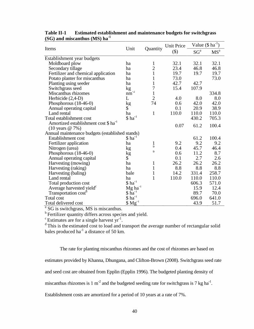
40
Table II-1 Estimated establishment and maintenance budgets for switchgrass (SG) and miscanthus (MS) ha-1
Items Unit Quantity Unit Price ($)
Value ($ ha-1) SGa MSa
Establishment year budgets Moldboard plow ha 1 32.1 32.1 32.1 Secondary tillage ha 2 23.4 46.8 46.8 Fertilizer and chemical application ha 1 19.7 19.7 19.7 Potato planter for miscanthus ha 1 73.0 73.0 Planting using seeder ha 1 42.7 42.7 Switchgrass seed kg 7 15.4 107.9 Miscanthus rhizomes nm-2 1 334.8 Herbicide (2,4-D) L 2 4.0 8.0 8.0 Phosphorous (18-46-0) kg 74 0.6 42.0 42.0 Annual operating capital $ 0.1 20.9 38.9 Land rental ha 1 110.0 110.0 110.0
Total establishment cost $ ha-1 430.2 705.3 Amortized establishment cost $ ha-1 (10 years @ 7%) 0.07 61.2 100.4
Annual maintenance budgets (established stands) Establishment cost $ ha-1 61.2 100.4 Fertilizer application ha 1 9.2 9.2 9.2 Nitrogen (urea) kg b 0.4 45.7 46.4 Phosphorous (18-46-0) kg b 0.6 11.2 8.7 Annual operating capital $ 0.1 2.7 2.6 Harvesting (mowing) ha 1 26.2 26.2 26.2 Harvesting (raking) ha 1 8.8 8.8 8.8 Harvesting (baling) bale 1 14.2 331.4 258.7 Land rental ha 1 110.0 110.0 110.0 Total production cost $ ha-1 606.3 571.0 Average harvested yieldc Mg ha-1 15.9 12.4 Transportation costd $ ha-1 89.7 70.0
Total cost $ ha-1 696.0 641.0 Total delivered cost $ Mg-1 43.9 51.7 a SG is switchgrass, MS is miscanthus. b Fertilizer quantity differs across species and yield. c Estimates are for a single harvest yr-1. d This is the estimated cost to load and transport the average number of rectangular solid bales produced ha-1 a distance of 50 km.
The rate for planting miscanthus rhizomes and the cost of rhizomes are based on
estimates provided by Khanna, Dhungana, and Clifton-Brown (2008). Switchgrass seed rate
and seed cost are obtained from Epplin (Epplin 1996). The budgeted planting density of
miscanthus rhizomes is 1 m-2 and the budgeted seeding rate for switchgrass is 7 kg ha-1.
Establishment costs are amortized for a period of 10 years at a rate of 7%.

41
For maintenance years (years 2 to 10), the only field operations are fertilizer
application and harvesting. The budgeted land rental rate of $110 ha-1 is based on the
average rental rate of non irrigated Oklahoma cropland of $75 ha-1 (Doye and Sahs 2009b)
plus a premium of $35 ha-1 to account for the anticipated market response to competition for
land in the electric plant’s vicinity.
The average price of coal delivered to the end use sector by census division (2007)
is given in Figure II-1. The U.S.A. price of coal varies from $14.36 Mg-1 in North Dakota
to $106.88 Mg-1 in New Jersey (DOE/EIA-0584 2009). The price of coal at which the
production of cellulosic biomass reaches a breakeven point is computed. A sensitivity
analysis is performed on selected parameter values (land rental rates, yields, machinery
costs, transportation costs, stand life, and input costs). A Mg of coal combusted to generate
electricity emits 3.48 Mg CO2 (Hong and Slatick 1994). This emission does not include the
carbon emitted by the mining and transportation activities required to get the coal to the
point of use. If the carbon emitted by machines involved in producing, harvesting, and
transporting biomass is ignored, the carbon sequestered in the plant material can be
assumed to be equivalent to the carbon released when biomass from perennial grasses is
combusted.
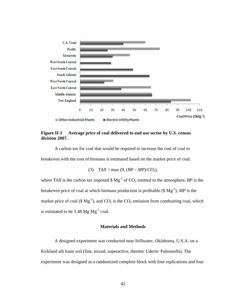
42
Figure II-1 Average price of coal delivered to end use sector by U.S. census division 2007.
A carbon tax for coal that would be required to increase the cost of coal to
breakeven with the cost of biomass is estimated based on the market price of coal:
(3) TAX = max (0, (BP – MP)/CO2)
where TAX is the carbon tax imposed $ Mg-1 of CO2 emitted to the atmosphere, BP is the
breakeven price of coal at which biomass production is profitable ($ Mg-1), MP is the
market price of coal ($ Mg-1), and CO2 is the CO2 emission from combusting coal, which
is estimated to be 3.48 Mg Mg-1 coal.
Materials and Methods
A designed experiment was conducted near Stillwater, Oklahoma, U.S.A. on a
Kirkland silt loam soil (fine, mixed, superactive, thermic Udertic Paleustolls). The
experiment was designed as a randomized complete block with four replications and four
43
plots per replication. Treatments consisted of two species, miscanthus (Miscanthus x
giganteus) and switchgrass (Panicum virgatum variety ‘Alamo’) and two harvest levels
(one yr-1 post senescence and two yr-1, July and post senescence). The four treatments,
each consisting of a species and harvest level combination, were assigned randomly to
plots with one combination of treatment in each replication. The plots were 2.44 m wide
and 6.10 m in length. Four rows were planted in each plot 0.61 m apart.
The grasses were planted on June 24-25, 2002. Biomass was harvested in 2003,
2004, and 2005. Summary statistics for selected weather variables are provided in
Table II-2. Annual dry-matter and gross energy (kJ gm-1) yield estimates were computed
from biomass harvested from the center two rows of each plot. A calorimeter was used
to determine the energy content. Summary statistics of yield and energy content are
provided in Table II-3.

44
Table II-2 Overview of weather during the experiment period at Stillwater, Oklahoma U.S.A. (2003-2005) Weather parameters 2003 2004 2005 Mean SD Min Max Mean SD Min Max Mean SD Min Max Rainfall (mm month-1) 56.1 32.0 2.03 106.4 77.7 62.2 5.8 230.6 64.3 62.2 0.0 222.8 Solar radiation (MJ m2) 15.8 6.10 7.2 25.2 15.6 5.7 6.8 22.6 16.3 6.2 7.3 25.6 Soil max. temperature (ºC) 30.7 -11.6 21.1 41.1 30.0 -12.4 22.2 36.7 31.1 -12.3 22.8 37.8 Soil min. temperature (ºC) 14.2 -9.0 2.8 27.2 14.4 -9.5 3.3 25.0 14.8 -9.2 3.3 26.1 Source (Mesonet 2007). Table II-3 Summary statistics of yield and energy content of biomass
Chapter III Chapter IV Biomass Yield (Mg ha-1 yr-1)
Gross Energy (kJ gm-1)
Species Harvest yr-1
Mean SD Min Max Mean SD Min Max
Miscanthus 1 12.39 1.87 9.27 14.56 16.11 1.62 13.27 17.79 2 13.04 1.64 11.27 15.97 15.65 2.02 11.16 17.56
Switchgrass 1 15.87 2.94 11.72 20.65 15.73 1.62 13.76 17.56 2 15.42 2.86 10.64 20.63 15.84 2.98 8.95 17.69
45
Statistical Analysis
Separate models are estimated for the treatment effects with biomass yield and
energy content as dependent variables. Statistical analysis is performed using the
PROC MIXED procedure of SAS (SAS 2009). In both models, the treatments (species
and harvest levels) are modeled as fixed effects and replication and year as random
effects. Treatment main effects and interaction effects are tested for significance. The
means are compared with LSMEANS and ESTIMATE statements. The complete data
generating processes to analyze the effect of treatments on biomass yield can be
stated as
where is the biomass yield expressed in Mg ha-1 yr-1, is the intercept term,
represents the effect of species (miscanthus and switchgrass), represents the
effect of the harvest level (once and twice yr-1), and is the species by
harvest interaction effect. The error term associated with blocking (replication) is
defined as where k =1, 2,…,4 represents the replications. The
experiment was continued through three harvest years (t =1, 2, and 3 represents years
2003, 2004, and 2005). Biomass yield depends on random weather effects during a
particular year, and represents the year random effect. The random
errors with each experimental unit as well as error terms associated
with replication and year ( are assumed to be independent and identically
distributed.
46
The quality (energy content) of biomass is also considered as a function of
species and harvest treatment. The data generating process for the energy equation
can be stated as
where is the energy content of the biomass, π is the intercept term, is the effect
of species, is the effect of harvest treatment, represents the interaction
effect, is the random effect with respect to replication, is the
random effect associated with year and is the random error term, and
the error terms are assumed to be independent and identically distributed.
Results
Results for the biomass yield and energy content models are given in Tables II-4
and II-5. The type 3 test for mixed effects confirms that biomass production is strongly
affected by species (P value < 0.001). The harvest levels and the interaction effects are
not significant (P value 0.87 and 0.36 respectively). Switchgrass produced a greater
biomass yield (15.64 Mg ha-1 yr-1) than miscanthus (12.72 Mg ha-1 yr-1). Across both
species mean biomass yield increased slightly (but not significantly) from 14.13 Mg ha-1
yr-1 to 14.23 Mg ha-1 yr-1 with an additional harvest. Mean switchgrass yield decreased
from 15.87 Mg ha-1 yr-1 to 15.42 Mg ha-1 yr-1 with an additional harvest. Switchgrass did
not recover well from a July harvest (USDA/NRCS 2008). This finding is consistent with
that of previous studies conducted in the region (McLaughlin and Walsh 1998;
Sanderson, et al. 1999; Aravindhakshan, Epplin, and Taliaferro 2008).

47
Table II-4 Results of the type III test for main effects and interactions for biomass yield and energy content as dependent variables.
Effects Biomass Yield Energy Content
F-value Type III P>F F-value Type III
P>F Species 23.39 <.0001 0.01 0.90 Harvest 0.03 0.87 0.05 0.82 Species * Harvest 0.82 0.36 0.15 0.71 Table II-5 Least squares mean values for biomass yield and energy content of biomass
Effects Biomass Yield (Mg ha-1 yr-1) Energy Content
(million kJ Mg-1) Species Miscanthus 12.72 15.88 Switchgrass 15.64 15.79 Harvest levels Harvest-1 14.13 15.92 Harvest-2 14.23 15.75 Treatment Interactions Miscanthus * Harvest-1 12.39 16.12 Miscanthus * Harvest-2 13.04 15.65 Switchgrass * Harvest-1 15.87 15.73 Switchgrass * Harvest-2 15.42 15.85
Tests for fixed effects reveal that none of the analyzed independent variables
(species and harvest levels) and their interaction effects significantly affect the energy
content of biomass. The least squares mean value for energy content of biomass was
higher for miscanthus (15.88 kJ gm-1). Harvesting twice rather than once yr-1 reduced the
mean energy content of the biomass, but not significantly. Miscanthus harvested once yr-1
after senescence produced the highest energy content (16.12 kJ gm-1). However, since
switchgrass produced a significantly greater biomass yield, the energy production per
land unit was greater with switchgrass.
48
The delivered cost of biomass (Tables II-3 and II-6) was lowest for switchgrass
harvested once yr-1 ($43.9 Mg-1). The delivered cost estimate is consistent with findings
of previous studies (McLaughlin and Kszos ($44 Mg-1 in 2005); Epplin ($37 Mg-1 in
1996); Aravindhakshan et al. ($39-$46 Mg-1 in 2008) (Epplin 1996; McLaughlin and
Walsh 1998; Aravindhakshan, Epplin, and Taliaferro 2008).
For a U.S.A. average coal price of $39.76 Mg-1, the value of switchgrass biomass
delivered to a cofiring plant as a substitute for coal, based on energy content, is estimated
to be $27.1 Mg-1 . This is an estimate of the maximum price that a profit maximizing
cofiring plant manager would offer for delivered biomass. This estimate does not
consider differences in external benefits and the costs of using biomass, and it does not
account for additional costs incurred for modifying the electric generation facility to
accommodate the biomass.
The objective of the farm operator is to obtain maximum net revenue ha-1 and as
per equations (1) and (2), that depends on the total energy produced ha-1. Based on results
of the field trials, for the region, the best strategy would be to establish switchgrass and
harvest once yr-1 after senescence. Switchgrass produced 50 million kJ ha-1 more energy
than miscanthus when harvested once yr-1. When harvested twice yr-1, the total energy
production ha-1 decreased (5.2 million kJ ha-1) for switchgrass. Even though harvesting
twice yr-1 slightly increases the yield for miscanthus (0.6 Mg ha-1), the revenue from the
second harvest is less than the additional cost of the second harvest, and the total net
revenue declines by $55 ha-1. Harvesting twice yr-1 is not an economically viable cultural
practice in the region for either species.
49
The cost of producing biomass is greater than the value based on the price of coal
(Table II-6). None of the treatment combinations would produce positive net revenue if
the biomass price was based on energy content relative to coal. For a coal price of $39.76
Mg-1 biomass production in the region from either switchgrass or miscanthus for cofiring
with coal is not financially feasible when the value is based on the energy content of
biomass.
Sensitivity of net revenue to changes in land rental rate, biomass yield, machinery
cost, transportation cost, input cost, and stand life is reported in Table II-7. If the
government permits the use of land currently in the Conservation Reserve Program at no
cost to produce feedstock such that the rental rate assigned to the production of feedstock
is assumed to be zero (Epplin 1996), the net revenue increases by 31-41% with more
response for switchgrass. However, even with a land cost of zero, producing biomass
from either species to substitute for coal does not generate positive returns.

50
Table II-6 Results of the feasibility analysis of biomass production in the U.S.A. Southern plains
Chapter V Harvest Level
Cost of Biomass ($ Mg-1) a
Total Energy (million kJ ha-1)
Value of Biomass Given a Coal Price of
$40Mg-1 ($ Mg-1) b Total Value
($ ha-1) Total Cost
($ ha-1) Net Value
($ ha-1)
Switchgrass 1 43.9 249.6 27.1 430.6 696.0 -265.4
Switchgrass 2 47.3 244.4 27.3 421.6 728.3 -306.7
Miscanthus 1 51.7 199.7 27.8 344.5 641.0 -296.5
Miscanthus 2 53.9 204.1 27.0 352.0 703.1 -351.0
a This is an estimate of the costs to produce, harvest, and deliver biomass a distance of 50 km. b The value of biomass is estimated based on its energy content relative to the price and energy content of coal.

51
Table II-7 Results of sensitivity analysis of net revenue
Chapter VI Switchgrass Harvest-1
Switchgrass Harvest-2
Miscanthus Harvest-1
Miscanthus Harvest-2
Net Revenue ($ ha-1)
% Change a
Net Revenue ($ ha-1)
% Change
Net Revenue ($ ha-1)
% Change
Net Revenue ($ ha-1)
% Change
Normal -265.4
-306.7
-296.5
-351.0 Without Land rental value -155.4 41% -196.7 36% -186.5 37% -241.0 31%
25% Increase in rent -292.9 -10% -334.2 -9% -324.0 -9% -378.5 -8% 25% Decrease in rent -237.9 10% -279.2 9% -269.0 9% -323.5 8% 25% Increase in yield -372.8 -40% -411.0 -34% -380.3 -28% -439.3 -25% 25% Decrease in yield -158.0 40% -202.4 34% -212.7 28% -262.8 25% 25% Increase in machinery cost -364.7 -37% -414.8 -35% -372.3 -26% -441.4 -26% 25% Decrease in machinery cost -166.0 37% -198.6 35% -220.7 26% -260.7 26% 25% Increase in transportation cost -287.8 -8% -328.5 -7% -314.0 -6% -369.5 -5% 25% Decrease in transportation cost -243.0 8% -284.9 7% -279.0 6% -274.2 22% 25% Increase in input cost -286.2 -8% -327.5 -7% -279.0 6% -332.6 5% 25% Decrease in input cost -244.6 8% -285.9 7% -267.5 10% -322.0 8% Stand life period 15 years -251.4 5% -292.7 5% -273.5 8% -328.1 7% Breakeven price of coal 64.3
68.7
74.0
79.4
Estimated carbon tax ($ Mg-1 CO2) West South Central b U.S.A. 10.2 11.5 13.0 14.6 U.S.A. 7.0 8.3 9.8 11.4
a The percentage change is calculated from the estimates of net revenue from Table II-6. b The market price of coal in West South Central is $28.67 Mg-1, and the average coal price in the U.S.A. is $39.76 Mg-1.

52
The net revenue is sensitive to yield fluctuations with a wide range of 25-40% for
different species harvest combinations. The cost of fertilizer application, harvest, and
transportation that depends on the yield accounts for $33 Mg-1 and is greater than the
price of the delivered biomass. If the value of biomass is less than $33, an increase in
yield would reduce the net revenue and increase the farm operator’s losses. Under such
price circumstances, if the perennial grass is established and the farmer cannot switch
crops, the best strategy would be to not apply fertilizer, not harvest, and not transport the
biomass. If the market price of biomass is less than variable production costs, increases in
yield will not make biomass production feasible. The share of the machinery costs
(custom rates) is high in the production of biomass, and the net revenue is sensitive (26-
37%) to the changes in the custom rates, which in turn shows that net revenue will be
sensitive to fuel and labor cost. The changes in input costs, transportation costs, and stand
life period of grasses do have comparatively small effects on the net revenue. The value
of biomass is estimated based on the energy content with reference to the energy and
price of coal. The price of coal shows a wide range and differs between the regions and
within the regions. With all other assumptions held constant, the price of coal at which
the production of biomass breakeven ranges from $64.3 Mg-1 to $79.4 Mg-1 for different
treatment combinations. For the U.S.A. average coal price of $39.76 Mg-1, the carbon tax
based on CO2 emission, required for cofiring switchgrass biomass with coal to breakeven
with using only coal is estimated to be $7 Mg-1 of CO2.
Table II-8 was prepared to illustrate the expected changes in cost to deliver
feedstock resulting from changes in biomass yield.
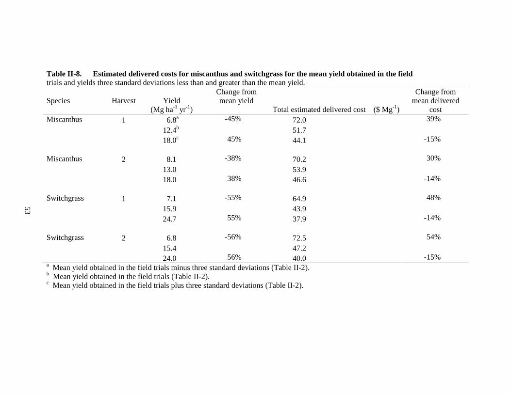
53
Table II-8. Estimated delivered costs for miscanthus and switchgrass for the mean yield obtained in the field trials and yields three standard deviations less than and greater than the mean yield.
Species Harvest Yield (Mg ha-1 yr-1)
Change from mean yield
Total estimated delivered cost ($ Mg-1)
Change from mean delivered
cost Miscanthus 1 6.8a -45% 72.0 39%
12.4b 51.7
18.0c 45% 44.1 -15%
Miscanthus 2 8.1 -38% 70.2 30%
13.0 53.9
18.0 38% 46.6 -14%
Switchgrass 1 7.1 -55% 64.9 48%
15.9 43.9
24.7 55% 37.9 -14%
Switchgrass 2 6.8 -56% 72.5 54%
15.4 47.2
24.0 56% 40.0 -15%
a Mean yield obtained in the field trials minus three standard deviations (Table II-2). b Mean yield obtained in the field trials (Table II-2). c Mean yield obtained in the field trials plus three standard deviations (Table II-2).
54
Based on the field trials the mean annual yield of 15.9 Mg ha-1 for switchgrass
when harvested once per year has an estimated standard deviation of 2.94 Mg ha-1. By
this measure a yield range from 7.1 to 24.7 Mg ha-1 is expected to include the yield
distribution from minus to plus three standard deviations. In the event of an extremely
low yield of 7.1 Mg ha-1, the expected delivered cost increases by 48% from $43.9 to
$64.9 Mg-1. For a biomass yield of 24.7 Mg ha-1 (three standard deviations greater than
the mean), the expected cost to deliver feedstock is decreased by 14% from $43.9 to
$37.9 Mg-1. Cost to deliver biomass is more sensitive to lower yields ha-1 than to greater
yields.
Discussion
Efforts have been underway for a number of years to develop energy crops for use
as biorefinery feedstocks for the production of liquid fuels including ethanol. The
development of technology required for economically viable conversion of cellulosic
biomass feedstocks to ethanol has not progressed as rapidly as promised, however,
substantial progress has been made in the development of switchgrass and miscanthus as
dedicated energy crops. In addition to providing feedstock for lignocellulosic
biorefineries, feedstocks such as switchgrass and miscanthus could be used to produce
biomass for cofiring with coal in existing electric generating plants.
The technology for cofiring with lignocellulosic biomass is simple, mature, and
requires only minor modifications of, and minimal investment in, existing plants.
Biomass is more expensive than coal and if the externalities of burning coal are ignored,
biomass feedstocks would be substantially more costly. A tax on carbon emissions could
be used to provide an incentive for cofiring with biomass. This study was conducted to

55
determine the minimum carbon tax required for either of the two candidate feedstocks
(miscanthus and switchgrass) to be economically viable alternatives for cofiring with
coal.
Annual dry-matter yield and gross energy (kJ gm-1) data were produced in side-
by-side experiment station trials conducted in Oklahoma U.S.A. Switchgrass with a
single annual post-senescence harvest produced more biomass (15.87 Mg ha-1 yr-1 versus
12.72 Mg ha-1 yr-1) and more energy (249.6 million kJ ha-1 yr-1 versus 199.7 million kJ
ha-1 yr-1) than miscanthus. For the average yields obtained, the estimated cost to produce
and deliver biomass an average distance of 50 km was $43.9 Mg-1 for switchgrass and
$51.7 Mg-1 for miscanthus. Based on the results of these field trials, the best strategy for
producing biomass in the region would be to establish switchgrass and harvest once yr-1
after senescence.
For the U.S.A average coal price of $39.76 Mg-1, the value of switchgrass
biomass delivered to a cofiring plant as a partial substitute for coal, based on energy
content is estimated to be $27.1 Mg-1. Replacing one Mg of coal with switchgrass
biomass reduces CO2 emission by 3.48 Mg. If a tax of $7 Mg-1 on CO2 were imposed,
cofiring switchgrass with coal would breakeven with using only coal for the average coal
price of $39.76 Mg-1.
In this study, switchgrass produces significantly more biomass than miscanthus.
The cost of producing a Mg of biomass is also substantially less for switchgrass than for
miscanthus. However, in other studies conducted at different locations, miscanthus has
produced more biomass than switchgrass. These findings confirm that the best species
and variety differ across climate and region. Prior to establishing thousands of acres of a

56
perennial grass in a given region for use as a dedicated energy crop, side-by-side trials of
competing species and varieties should be conducted to confirm the most economical
species and variety for the region.
Finally, a comprehensive strategy to address greenhouse gas emissions would
consider several additional issues. As noted, greenhouse gases other than CO2 and
greenhouse gases used to establish, produce, fertilize, and harvest the grasses, mine the
coal, and transport the biomass and coal to the point of use were not considered. Since
miscanthus must be propagated vegetatively whereas switchgrass may be propagated
from seeds, it could be hypothesized that the greenhouse gas emissions from growing the
two species are different. When perennial grasses are established on depleted cropland,
they will sequester carbon in the soil. Public policy that taxes carbon emissions might
also compensate land owners for sequestering carbon. This compensation could be used
to offset some of the cost to deliver biomass feedstock. The quantity of carbon
sequestered was not measured in the field trials and differences in the quantity of carbon
sequestered across the species and harvest frequency were not determined. Additional
research would be required to determine the overall net differences in greenhouse gas
emissions between the two grasses and between the grasses and coal.

57
PAPER II REFERENCES
Aravindhakshan, S.C., F.M. Epplin, and C. Taliaferro. 2008. “Biomass Yield to Nitrogen Response Functions for Four Candidate Biorefinery Feedstock Perennial Grass Species.” AAEA annual meetings, Orlando FL, 27-29 July.
Clifton-Brown, J.C., I. Lewandowski, B. Andersson, G. Basch, D.G. Christian, J.B. Kjeldsen, U. Jorgensen, J.V. Mortensen, A.B. Riche, K Schwarz, K Tayebi, and F Teixeira. 2001. “Performance of 15 Miscanthus Genotypes at Five Sites in Europe.” Agronomy Journal 93:1013-19.
Downing, M., and R.L. Graham. 1996. “The Potential Supply Cost of Biomass from Energy Crops in the Tennessee Valley Authority Region.” Biomass and Bioenergy 11(4):283-303.
Doye, D., and R.Sahs. 2009a. “Oklahoma Farm and Ranch Custom Rates, 2007-08.” Oklahoma state university, Oklahoma Coop. Ext. Ser., Accessed on September 2009 from <http://osufacts.okstate.edu >
______. 2009b. CR-230 0207 “Oklahoma Cropland Rental Rates: 2006-07.” Oklahoma state university, Oklahoma Coop. Ext. Ser., Accessed on September 2009 from <http://osufacts.okstate.edu >
English, B.C., C. Short, and E.O. Heady. 1981. “The Economic Feasibility of Crop Residues as Auxiliary Fuel in Coal-Fired Power Plants.” American Journal of Agricultural Economics 63(4):636-644.
Epplin, F.M. 1996. “Cost to Produce and Deliver Switchgrass Biomass to an Ethanol-Conversion Facility in the Southern Plains of the United States.” Biomass and Bioenergy 11(6):459-467.
Fike, J.H., D.J. Parrish, D.D. Wolf, J.A. Balasko, J.T. Green Jr, Rasnake M, and J.H. Reynolds. 2006. “Switchgrass Production for the Upper Southeastern USA: Influence of Cultivar and Cutting Frequency on Biomass Yields.” Biomass and Bioenergy 30:207-213.
Fischer, G., S. Prieler, and H.V. Velthuizen. 2005. “Biomass Potentials of Miscanthus, Willow and Poplar: Results and Policy Implications for Eastern Europe, Northern and Central Asia.” Biomass and Bioenergy 28(2):119-132.
58
Fraas, A.G., and R.C. Johansson. 2009. “Conflicting Goals: Energy Security vs. GHG Reductions Under the EISA Cellulosic Ethanol Mandate.” Resources for the Future Discussion Paper No. 09-24 Washingto D.C.
Fuentes, R.G., and C.M.Taliaferro. 2002 “Biomass Yield Stability of Switchgrass Cultivars.” In: J. Janick, and A. Whipkey, eds. Trends in New Crops and New Uses. Alexandria VA: ASHS Press.
Heaton, E., T.Voigt, and S.P. Long. 2004. “A Quantitative Review Comparing the Yields of Two Candidate C4 Perennial Biomass Crops in Relation to Nitrogen, Temperature and Water.” Biomass and Bioenergy 27:21-30.
Hong, B.D., E.R. Slatick. 1994. Carbon Dioxide Emission Factors for Coal. Quarterly Coal Report, Energy Information Administration, January-April 1994, pp. 1-8. Accessed on November 2009 from <http://www.eia.doe.gov/cneaf/coal/quarterly/co2_article/co2.html>
Jorgensen, U. 1997. “Genotypic Variation in Dry Matter Accumulation and Content of N, K, and Cl in Miscanthus in Denmark.” Biomass and Bioenergy 12(3):155-69.
Khanna, M. 2008. “Cellulosic Biofuels: Are They Economically Viable and Environmentally Sustainable?” Choices 23(3):16-20.
Khanna, M., B. Dhungana, and J. Clifton-Brown. 2008 “Costs of Producing Miscanthus and Switchgrass for Bioenergy in Illinois.” Biomass and Bioenergy 32(6):482-493.
Lewandowski, I., and A. Kicherer. 1997. “Combustion Quality of Biomass: Practical Relevance and Experiments to Modify the Biomass Quality of Miscanthus x giganteus.” European Journal of Agronomy 6(3-4):163-177.
Lewandowski, I., J.M.O. Scurlock, E. Lindvall, and M. Christou. 2003. “The Development and Current Status of Perennial Rhizomatous Grasses as Energy Crops in the US and Europe.” Biomass and Bioenergy 25(4):335-361.
McLaughlin, S.B., and M.E. Walsh. 1998. “Evaluating Environmental Consequences of Producing Herbaceous Crops for Bioenergy.” Biomass and Bioenergy 14(4):317-324.
Mesonet. 2007. Accessed on August 2009 from <http://www.mesonet.org/>
Olsen, A. 2001. “Co-burning Biomass Opportunities in Wisconsin A Strategic Assessment.” Division of Energy, Wisconsin Dept. of Adm. Final report for Contract No. 8008, June.
Perlack, R.D., L.L. Wright, A.F. Turhollow, R.L. Graham, B.J. Stokes, and D.C. Erbach. 2005. Biomass as Feedstock for a Bioenergy and Bioproducts Industry: the

59
Technical Feasibility of a Billion-Ton Annual Supply.Washington, DC: U.S. Department of Agriculture, U.S. Department of Energy.
Sanderson, M.A., J.L. Read, W.R. Ocumpaugh, M.A. Hussey, E.G. Van, J.C. Read, C. R. Tischler, and F.M. Hons. 1999. “Switchgrass Cultivars and Germplasm for Biomass Feedstock Production in Texas.” Bioresource Technology 67:209–219.
SAS. 2009. SAS System under MICROSOFT Windows. Release 9.1. Cary NC: SAS Institute Inc.,
Sladden, S.E., D.I. Bransby, and G.E. Aiken. 1991. “Biomass Yield, Composition and Production Costs for Eight Switchgrass Varieties in Alabama.” Biomass and Bioenergy 1(2):119-122.
U.S. Department of Agriculture (USDA/NRCS). 2008. Plant Materials Program. Accessed from http://plant-materials.nrcs.usda.gov, August.
U.S. Department of Energy (DOE/EIA). 2009. Coal 2009. Washington, DC, Accessed on November 2009 from <http://www.energy.gov/energysources/coal.htm>.
U.S. Department of Energy (DOE/EIA-0035). 2009. Approximate Heat Content of Coal and Coal Coke , 1949-2008. Washington, DC, Accessed on September 2009, from <http://www.eia.doe.gov/emeu/aer/txt/ptb1305.html >
U.S. Department of Energy (DOE/EIA-0573). 2007. Emissions of Green House Gases in the United States 2007. Washington, DC Accessed on January 2010, from <http://www.eia.doe.gov/oiaf/1605/ggrpt/pdf/0573(2007).pdf>.
U.S. Department of Energy (DOE/EIA-0584). 2009. Average Price of Coal Delivered to End Use Sector by Census Division and State, 2008, 2007. Washington, DC Accessed on October 2009, from <http://www.eia.doe.gov/cneaf/coal/page/acr/table34.html>
Vocke, G., and E. Allan. 2006. Wheat Situation and Outlook Yearbook. Electronic outlook report from the Economic Research Service. Washington D.C. U.S. Department of Agriculture.

60
Chapter VII
PAPER III
IDENTIFYING JUMPS AND SYSTEMATIC RISK IN FUTURES
Abstract
A variety of multivariate jump-diffusion models have been suggested as models
of asset prices. This paper extends the literature on (joint) mixed jump-diffusion
processes in futures markets by using the CRB index futures to represent systematic risk
in commodity prices. We derive (joint) mixed bivariate normal distributions and
likelihood functions for estimating the parameters of jump-diffusion processes.
Likelihood ratio tests are used to select among nested models. The empirical results show
the presence of downside jumps and significant systematic risk in wheat futures returns.
Amin and Ng’s (1993) model with a single counter of jumps fits better than other jump-
diffusion processes considered. The jump components did not have significantly more
systematic risk than the continuous component. In terms of wheat prices, one standard
deviation jumps are 14 cents per bushel and two standard deviation jumps are 29 cents
per bushel and are within the price limits. These jumps occur once in every six business
days and are mostly crashes.

61
Introduction
Previous studies show that futures returns have occasional large movements that
result in asymmetric and leptokurtic distributions (Hudson, Leuthold and Sarassoro 1987;
Hall, Brorsen, and Irwin 1989; Koekebakker and Gudbrand 2004). In this paper futures
returns is defined as the percentage change in value from the closing price on one trading
day to the closing price on the next trading day of a single contract. Since the quantity of
a contract is fixed, the percentage change in price is equal to the percentage change in
value. Discontinuous jumps in asset prices and time-varying volatility models are the two
main approaches used to model extraordinary discrete price movements (Eraker 2004). In
Merton’s (1976) jump diffusion (JD) process, these price changes occur at discrete
points in time. The two weaknesses of the JD process that have been widely discussed in
the literature are: (1) the model has only a single counter1
1 Mathematically a counter process defines the number of arrivals that have occurred in the interval (0,t).
of jumps and (2) the jump
component represents only non-systematic risk and therefore a maintained hypothesis of
the model is that all jump risk can be diversified. Empirical studies show high correlation
between individual stock price volatility and market volatility (Jarrow and Rosenfeld
1984; Jorion 1988). If jumps in an individual asset are correlated with jumps in the
overall market, then contrary to the maintained hypothesis of Merton’s model, jump risk
is systematic and could not be diversified. Amin and Ng (1993) derived an option pricing
formula to account for stock return volatility that is both systematic and stochastic. In this
model, the number of jumps in the consumption and asset price process are identical and
are allowed to be correlated.
62
Camara’s (2009) theoretical “two counters of jumps” model is a joint JD process
of aggregate consumption and stock price. In this model, the jumps are separated into
upside (bubbles) and downside (crashes) jumps with different intensity and distributional
characteristics. Theoretically, Camara (2009) was able generalize Merton (1976) and
Amin and Ng (1993) using “two counters of jumps” model. In this extended model,
Camara (2009) included additional jump parameters in stock price and aggregate
consumption. Camara’s model, however has a potential estimation problem as it includes
sixteen jump parameters along with other parameters that represent continuous price
movements. As per Kou (2002) having so many parameters in the model makes
calibration difficult. In addition, if the jump magnitudes are small, the separation of
jumps from continuous co-movements and estimation of parameters becomes less precise
(Todorov and Bollerslev 2010). To circumvent this empirical problem, this paper
includes four JD processes with fewer parameters that are nested in Camara’s (2009) two
counters of jumps model. The criteria2
In Merton’s (1976) model, jumps are firm specific and are not correlated with the
stocks in general (i.e., with the market). It is clear from the 1987 stock market crash that
extreme events can influence all asset prices and market events. Similarly, commodities
and commodity futures are systematically related to macroeconomic measures and the
that are used in the selection of models are: (1) the
model should be able explain the asymmetric and leptokurtic nature of returns, (2) the
model should have an economic interpretation and practical implications, and (3) the
likelihood function of the distribution should be mathematically tractable to compute the
parameter estimates.
2 For detailed description of criteria, see Kou (2002).
63
risk associated with jumps cannot be diversified (Hilliard and Reis 1999). The nature of
the risk associated with jumps is not explicitly stated in Camara’s (2009) model.
Restricting the two counters of jumps model to have no jumps in consumption and single
counter of jumps in stock price results in the JD economy of Merton (1976) with non-
systematic jumps. The JD process of Amin and Ng (1993) with systematic jumps can be
obtained by assuming a single counter of jumps in consumption and stock price. In the
capital asset pricing model (CAPM) only systematic risk is rewarded. The current paper
includes a joint jump diffusion process that also represents the extended one factor model
of Todorov and Bollerslev (2010) with returns associated with continuous and
discontinuous price moves. The model also allows to test whether the betas associated
with these price moves are same. This more recently described JD process that includes
both systematic and non-systematic jumps was published subsequent to Camara’s (2009)
paper.
The inelastic demand and dependence on weather increases the chance of
extraordinary price movements in agricultural commodities. Some discrete incidence of
large price changes is confined to a single commodity. For example, freeze damage in
wheat may cause an extraordinary price change in wheat yet have little influence on other
commodity prices. These firm (commodity) specific events result in non-systematic
jumps in the returns. On the other hand, influences of macroeconomic variables like
exchange rate fluctuations affect prices of all commodities and are systematic. In
addition, Todorov and Bollerslev (2010) argued that the precision of beta estimates
increases with less incidence of non-systematic risk. The current paper extends Amin and
Ng (1993) by adding an uncorrelated jump to futures prices. We extend the futures
64
literature by specifying a joint JD process with a single counter of jumps in market prices
and two counters of jumps in futures prices. For the futures JD process, the jumps are
defined with separate Poisson processes to represent systematic and non-systematic
jumps. The model supports Todorov and Bollerslev’s (2010) theoretical framework that
extends the generic CAPM model to have two separate betas to represent the systematic
risk attributable to continuous and discontinuous price moves.
The empirical objective of the paper is to select the most suitable JD process to
model wheat futures prices and to estimate the systematic risk associated with the
continuous and discontinuous components. In the current paper, we consider alternative
stochastic processes that are nested in Camara’s (2009) two counters of jumps model and
estimate the parameters of the distributions. We contributes to the existing literature on
futures by proposing a mixed bivariate normal distribution for simultaneously analyzing
the price series. Both the continuous movements and the discrete movements in each
price series are modeled using normal and Poisson process respectively. This joint JD
process includes correlated and uncorrelated jumps and models the interaction between
wheat futures returns and commodity market returns. In addition, the paper also estimates
the parameters of mixed univariate normal distributions with single and two counters of
jumps in futures prices.
Jump diffusion processes that models systematic risk has several practical
applications in portfolio and credit risk management. As the jumps are correlated with
large number of assets, the presence of systematic risk reduces the gains from
diversification and substantially increases the probability to loose while holding highly
levered positions (Das and Uppal 2004). According to Duffie and Pan (2001), systematic
65
movements also influence the credit risk as all credits exhibit correlated default risk
during financial crisis. Duffie and Pan (2001) used a jump-conditional value at risk
(VaR) weighted by the probability of a given number of jumps for the analytical
approximation of VaR. Jumps across the assets are systematic even in the commodity
markets that makes it extremely difficult for grain trading firms to hedge the risk during
large correlated price movements.
Maximum likelihood is used to estimate the parameters of the diffusion process
using the Kansas City Board of Trade (KCBT) wheat futures prices and the Commodity
Research Bureau (CRB) index of futures prices. The Amin and Ng (1993) and Camara
(2009) models are extensions of the consumption-based representative agent framework.
In empirical analysis market prices are used instead of consumption growth (Amin and
Ng, 2003). In this paper the CRB index of futures prices represent the ‘commodity
market’. The empirical results show the presence of downside jumps and systematic jump
risk in wheat futures prices. Amin and Ng’s (1993) model fits the data better than other
JD processes considered. The differences in beta estimates of continuous and
discontinuous price moves were not statistically significant and failed to support Todorov
and Bollerslev’s (2010) extended CAPM framework.
Theoretical Model
This section introduces JD processes followed by univariate and bivariate mixed
normal distribution functions to model wheat futures prices, CRB index of futures prices
and estimate the distribution parameters. All JD processes included in this section are
restricted models of Camara’s (2009) two counters of jump process. We now outline the
stochastic process of asset price followed by the JD process with a single counter and

66
then with two counters of jumps. Let the asset price ) be a stochastic process with no
discrete jumps so it can be represented as
where is the current futures price, is standard Brownian motion, is
the instantaneous expected price without any jumps, and is the instantaneous variance
of price without any jumps. The asset price is assumed to be non-negative and the
period return (logarithmic price relative) is normally distributed as
where is the me is the mean (drift) and is the
variance. In the return series, the jump magnitude is normally distributed with expected
value of jump size and variance .
Univariate Mixed JD Process with Single Counter of Jumps
The number of extraordinary price changes follows a Poisson counting process
with mean arrival rate (intensity) and jump size . The magnitude of jumps can
be either positive (upside jumps) or negative (downside jumps). The JD process that
includes both continuous and discontinuous changes in prices is
In equation (2), the Brownian motion is a continuous process and the Poisson process is
discontinuous. It is assumed that and , and that and , and that
and are independent. The model reduces to geometric Brownian motion when there

67
are no jumps. As per Jorion (1988), the probability density function of a mixed univariate
normal distribution and a single counter of jumps is
Univariate Mixed JD Process with Two Counters of Jumps
Camara (2009) postulated a bivariate model with two separate Poisson distributed
events to represent upside jump and downside jumps. A univariate version of this richer,
potentially more realistic and less restricted jump-diffusion process with two counters of
jumps is
where and represent the upside jump and downside jump sizes,
respectively, is the Poisson counter process for upside jumps with intensity , and
is the Poisson counter process of downside jumps with intensity . In the price
(logarithmic price relative) series, both jumps are normally distributed and can have
different distributions each with different mean and variance. These price jumps can be
represented as and where, and are the
means and and are the variances of upside and downside jumps respectively.
For empirical estimation, the mean of upside jumps is restricted to be positive and
the mean of downside jumps is restricted to be negative. In this model, the jump
magnitudes are allowed to be correlated only if and
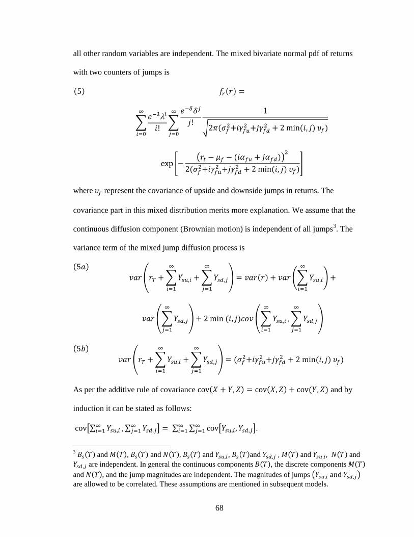
68
all other random variables are independent. The mixed bivariate normal pdf of returns
with two counters of jumps is
where represent the covariance of upside and downside jumps in returns. The
covariance part in this mixed distribution merits more explanation. We assume that the
continuous diffusion component (Brownian motion) is independent of all jumps3
. The
variance term of the mixed jump diffusion process is
As per the additive rule of covariance and by
induction it can be stated as follows:
.
3 and , and and , and and and
are independent. In general the continuous components , the discrete components and , and the jump magnitudes are independent. The magnitudes of jumps are allowed to be correlated. These assumptions are mentioned in subsequent models.

69
The minimum operator is to ensure equal number of jump magnitudes to
carry out the estimation of covariance4
Multivariate Mixed JD Process with Systematic Jumps
. A JD process with separate upside and downside
jumps is not a new concept in the financial literature. Kou (2002) proposed a double
exponential jump diffusion (DEJD) model. In the DEJD model, the jumps are generated
by a single Poisson process, and the upside and downside jump magnitudes are drawn
from two independent exponential distributions. Later Ramezani and Zeng (2007) posited
a Pareto-Beta jump-diffusion (PBJD) model in which the jumps are generated by two
independent Poisson processes and the jump magnitudes are drawn from Pareto and Beta
distributions respectively. In DEJD and PBJD, the distributions are univariate and the
relationship with the market is not defined as in Camara’s (2009) model. But, unlike
Camara (2009), they do not restrict positive jumps to be positive and negative jumps to
be negative.
The JD processes that are described in the above subsections were univariate
processes of asset prices. In these models, the influence of aggregate consumption on
asset price is not defined and implicitly assume non-systematic jumps. Camara’s (2009)
two counters of jumps model as a joint JD process of asset price and aggregate
consumption is
4 The sample covariance of two variables X and Y each with sample size n is
.

70
where is the Poisson counter process attributed to the incidence of upside jumps
with intensity , is the Poisson counter process attributed to the incidence of
downside jumps with the intensity parameter , is the current level of
consumption, is the consumption Brownian motion, is the instantaneous
expected growth rate of consumption without any jumps, is the variance of
consumption without any jumps, and and are the upside and downside jump
magnitudes in the aggregate consumption. In this model, the aggregate consumption
Brownian motion and asset price Brownian motion are correlated. The model also allows
jump components to be correlated5
Restricting Camara’s (2009) model to a single counter of jumps achieves the JD
economy of Amin and Ng (1993). In their model, the jumps in the asset price are
correlated with the jumps in aggregate consumption. The arrival of information in both
series is defined by a single Poisson counting process with intensity and the
number of jumps in both series are the same. The joint mixed JD process with a single
counter of jumps is
.
5 For more details of (auto)correlations between the jumps, see Camara (2009)
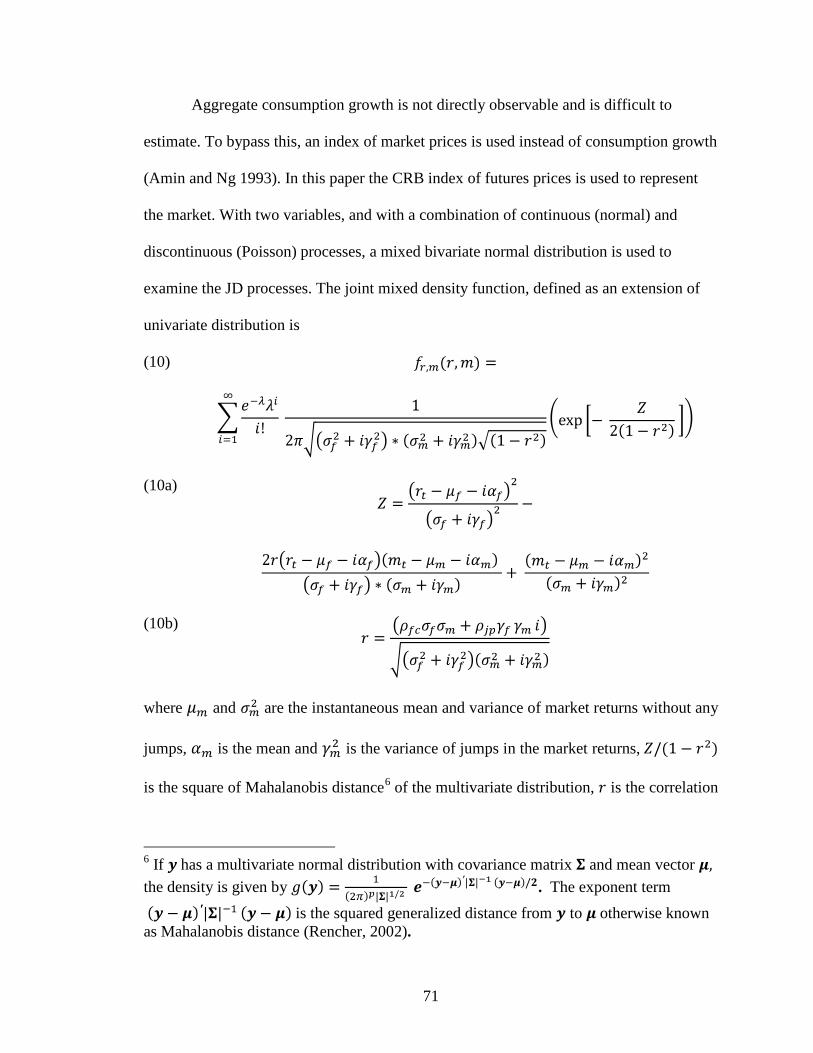
71
Aggregate consumption growth is not directly observable and is difficult to
estimate. To bypass this, an index of market prices is used instead of consumption growth
(Amin and Ng 1993). In this paper the CRB index of futures prices is used to represent
the market. With two variables, and with a combination of continuous (normal) and
discontinuous (Poisson) processes, a mixed bivariate normal distribution is used to
examine the JD processes. The joint mixed density function, defined as an extension of
univariate distribution is
(10)
(10a)
(10b)
where and are the instantaneous mean and variance of market returns without any
jumps, is the mean and is the variance of jumps in the market returns,
is the square of Mahalanobis distance6
6 If has a multivariate normal distribution with covariance matrix and mean vector the density is given by . The exponent term
is the squared generalized distance from to otherwise known as Mahalanobis distance (Rencher, 2002).
of the multivariate distribution, is the correlation
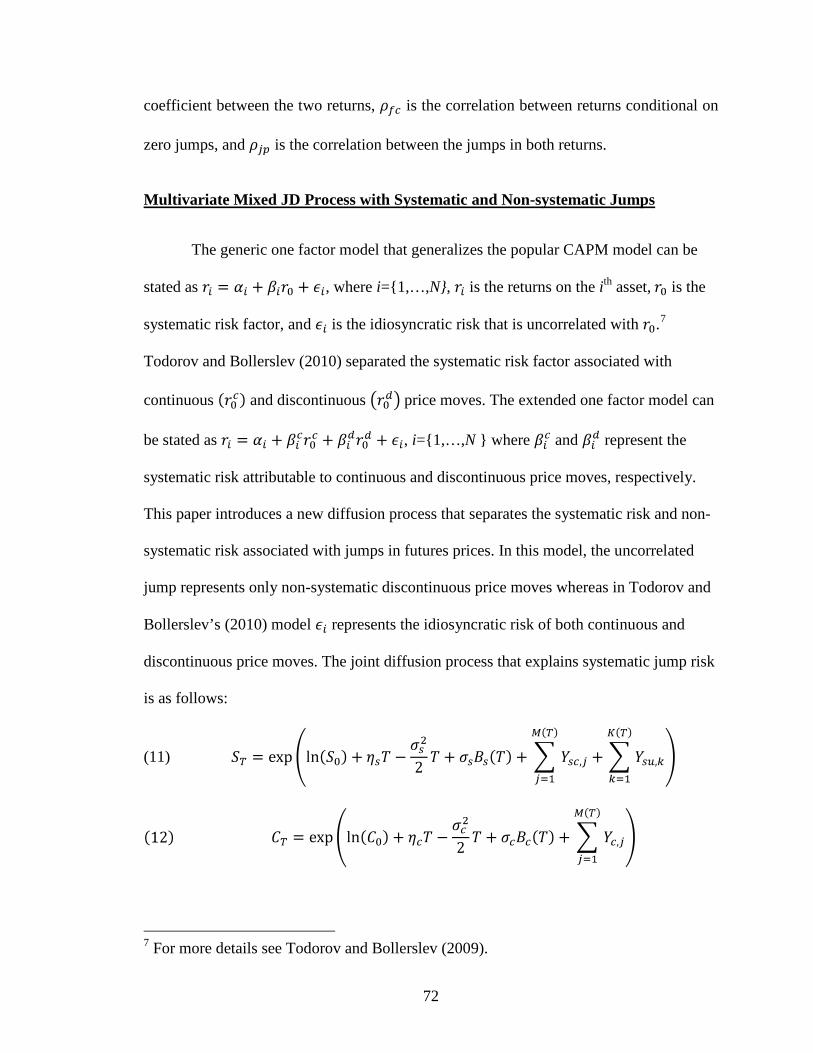
72
coefficient between the two returns, is the correlation between returns conditional on
zero jumps, and is the correlation between the jumps in both returns.
Multivariate Mixed JD Process with Systematic and Non-systematic Jumps
The generic one factor model that generalizes the popular CAPM model can be
stated as , where i={1,…,N}, is the returns on the ith asset, is the
systematic risk factor, and is the idiosyncratic risk that is uncorrelated with .7
(11)
Todorov and Bollerslev (2010) separated the systematic risk factor associated with
continuous and discontinuous price moves. The extended one factor model can
be stated as , i={1,…,N } where and represent the
systematic risk attributable to continuous and discontinuous price moves, respectively.
This paper introduces a new diffusion process that separates the systematic risk and non-
systematic risk associated with jumps in futures prices. In this model, the uncorrelated
jump represents only non-systematic discontinuous price moves whereas in Todorov and
Bollerslev’s (2010) model represents the idiosyncratic risk of both continuous and
discontinuous price moves. The joint diffusion process that explains systematic jump risk
is as follows:
7 For more details see Todorov and Bollerslev (2009).

73
where represents the jump in asset price that is correlated with the market jumps
, the Poisson counting process that is attributed to the incidence of correlated jumps
is with intensity . The non-systematic jump magnitude in the asset prices (
is modeled as the second Poisson counting process in the futures prices with an
intensity parameter . The correlated jump and uncorrelated jump are analogous to
and respectively. Hence, in equation (11), it is assumed that the magnitude of
systematic and non-systematic asset price jumps are not correlated
. The corresponding joint mixed bivariate normal
distribution is
(13a)
(13b)
where and are means, and are the variance of correlated and uncorrelated
jumps. The betas associated with continuous price moves and discontinuous price moves
are and respectively. The likelihood expressions
for the distribution functions are given in Appendix 1.
74
Data and Procedure
Summary statistics were estimated and normality tests were performed for both returns
series. The parameters of four increasingly general JD processes were estimated using
numerical maximization of likelihood functions. Two univariate mixed normal
distributions are estimated separately for each returns series with single and two counters
of jumps. Likelihood ratio (LR) tests are used to select among nested models. Finally, the
parameters of a joint mixed bivariate distribution with correlated single counter of jumps
in both returns, and the model with separate systematic and non-systematic jumps in
wheat futures prices are also estimated. Proc NLMIXED in SAS is used to estimate the
parameters (SAS 2009). To optimize the likelihood function, the infinite sum has to be
truncated to provide accuracy for parameter estimates (Jorion 1998). In this paper, the
infinite sum is truncated at ten. An extensive Monte Carlo simulation was performed to
ensure accuracy and reliability of statistical programs and procedures. Data were
simulated (100,000 observations) from the JD models known assumed parameter values.
After the likelihood optimization, the resulting values are identical or sufficiently close to
the assumed values.
The Kansas City Board of Trade (KCBT 2010) daily settlement wheat futures
prices were used for a period of six years (January 2003 to December 2008). Five wheat
futures contract maturity months (March, May, July, September, and December) are
traded. The last trading day is the business day preceding the fifteenth calendar day of the
liquidating month. The first delivery day is the first business day of the liquidating
month. The delivery mechanism is physical by using registered warehouse receipts from
elevators. A time-series dataset is constructed with the daily prices of actively traded
75
futures contract nearest to the twentieth calendar day of the month prior to delivery. From
the twenty-first calendar day onwards, the price of the next contract closest to the
delivery month in included in the dataset. This procedure reduces the maturity effect by
only including contracts close to maturity. It also avoids the delivery period where
position limits are removed and markets get thin. Differencing is performed before
splicing the data for rollover to avoid creating outliers at the rollover.
A synchronous data set of the Thomson Reuters/Jefferies CRB index is
constructed for the same time period. The CRB index is composed of four groups of
nineteen components that include petroleum products, metals, and agricultural
commodities. In the current study, CRB index futures represent the ‘commodity market’
(aggregate consumption) and the logarithmic price relatives as market returns (aggregate
consumption growth). Wheat, with an index weight of 1%, is in group IV along with
nickel, lean hogs, orange juice, and silver. The six expiration months traded are January,
February, April, June, August, and November. Actively traded futures are selected based
on the volume traded. The sixth calendar day of the month prior to the maturity month is
selected as the rollover day. The daily closing price of index futures is used to estimate
trading day to trading day changes in the value of the underlying assets. The differencing
to calculate returns is performed before splicing the data. Both the CRB and wheat series
include 1,380 observations of daily prices so as to provide enough degrees of freedom to
use tests that are asymptotically valid. To reduce scaling problems, differences in daily
prices are multiplied by 100 and expressed in percentage terms.

76
Empirical Results
Table III-1 presents summary statistics and tests of normality. The positive excess
kurtosis in both series indicates the presence of fat tails. The skewness of the wheat
futures price differences series is close to zero while the CRB index shows considerable
negative skewness.
Table VII-1. Summary statistics and normality tests for the returns Parameters Wheat Futures CRB index Minimum change in daily value -8.451 -6.406 Maximum change in daily value 7.778 5.429 Mean change in daily value 0.023 a 0.009 Variance 3.636 1.049 Skewness 0.049 -0.755 Excess kurtosis 1.735 5.137 Kolmogorov-Smirnov D statistic 0.045
(<0.01)b 0.076
(<0.01) Shapiro-Wilk W statistic 0.981
(<0.0001) 0.932
(<0.0001) a The returns are expressed in percentages and the number of observations is 1,380.The beginning date of the data series is January 2003 and the ending date is December 2008. b P-values are in the parentheses.
The normality tests (Kolmogorov-Smirnov D statistic and Shapiro-Wilk W
statistic) reject the null hypotheses at conventional levels of significance and make it
clear that the returns are not normally distributed. The estimates of second and third
moments and results of normality tests suggest that a JD process can provide a better fit
for the returns than a normal distribution.
The parameter estimates and standard errors of jump diffusion processes with a
single counter of jumps (equations (2) and (3)) are displayed in table III-2. The jump
intensity parameter is significant in both returns.
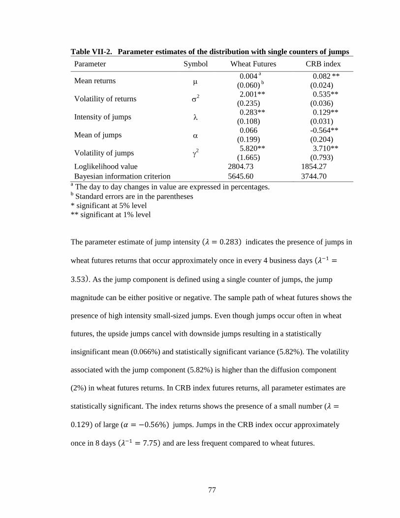
77
Table VII-2. Parameter estimates of the distribution with single counters of jumps Parameter Symbol Wheat Futures CRB index
Mean returns µ 0.004 a (0.060) b
0.082 ** (0.024)
Volatility of returns σ2 2.001** (0.235)
0.535** (0.036)
Intensity of jumps λ 0.283** (0.108)
0.129** (0.031)
Mean of jumps α 0.066 (0.199)
-0.564** (0.204)
Volatility of jumps γ2 5.820** (1.665)
3.710** (0.793)
Loglikelihood value 2804.73 1854.27 Bayesian information criterion 5645.60 3744.70
a The day to day changes in value are expressed in percentages. b Standard errors are in the parentheses * significant at 5% level ** significant at 1% level
The parameter estimate of jump intensity indicates the presence of jumps in
wheat futures returns that occur approximately once in every 4 business days
. As the jump component is defined using a single counter of jumps, the jump
magnitude can be either positive or negative. The sample path of wheat futures shows the
presence of high intensity small-sized jumps. Even though jumps occur often in wheat
futures, the upside jumps cancel with downside jumps resulting in a statistically
insignificant mean (0.066%) and statistically significant variance (5.82%). The volatility
associated with the jump component (5.82%) is higher than the diffusion component
(2%) in wheat futures returns. In CRB index futures returns, all parameter estimates are
statistically significant. The index returns shows the presence of a small number (
of large ( jumps. Jumps in the CRB index occur approximately
once in 8 days and are less frequent compared to wheat futures.
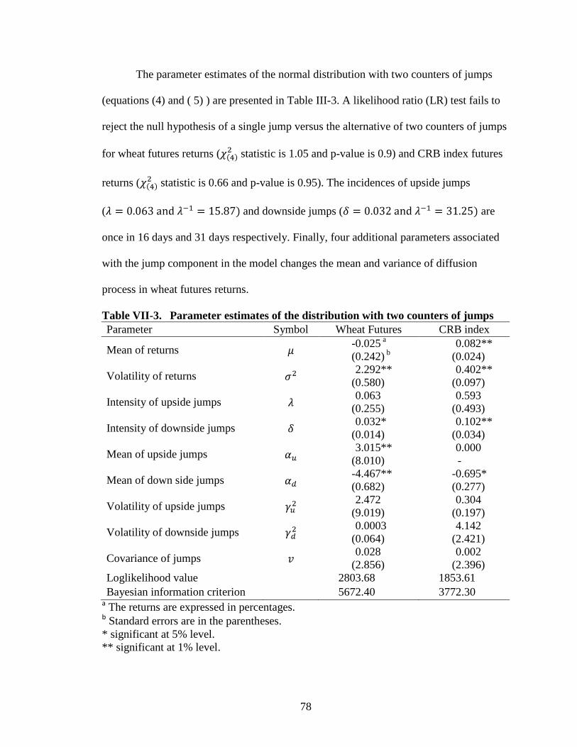
78
The parameter estimates of the normal distribution with two counters of jumps
(equations (4) and ( 5) ) are presented in Table III-3. A likelihood ratio (LR) test fails to
reject the null hypothesis of a single jump versus the alternative of two counters of jumps
for wheat futures returns ( statistic is 1.05 and p-value is 0.9) and CRB index futures
returns ( statistic is 0.66 and p-value is 0.95). The incidences of upside jumps
( and downside jumps ( are
once in 16 days and 31 days respectively. Finally, four additional parameters associated
with the jump component in the model changes the mean and variance of diffusion
process in wheat futures returns.
Table VII-3. Parameter estimates of the distribution with two counters of jumps Parameter Symbol Wheat Futures CRB index
Mean of returns -0.025 a (0.242) b
0.082** (0.024)
Volatility of returns 2.292** (0.580)
0.402** (0.097)
Intensity of upside jumps 0.063 (0.255)
0.593 (0.493)
Intensity of downside jumps 0.032* (0.014)
0.102** (0.034)
Mean of upside jumps 3.015** (8.010)
0.000 -
Mean of down side jumps -4.467** (0.682)
-0.695* (0.277)
Volatility of upside jumps 2.472 (9.019)
0.304 (0.197)
Volatility of downside jumps 0.0003 (0.064)
4.142 (2.421)
Covariance of jumps 0.028 (2.856)
0.002 (2.396)
Loglikelihood value 2803.68 1853.61 Bayesian information criterion 5672.40 3772.30
a The returns are expressed in percentages. b Standard errors are in the parentheses. * significant at 5% level. ** significant at 1% level.
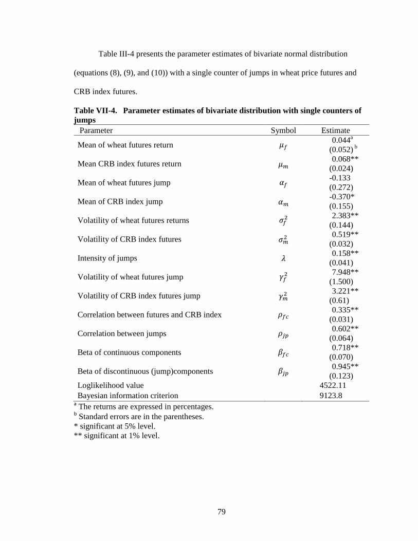
79
Table III-4 presents the parameter estimates of bivariate normal distribution
(equations (8), (9), and (10)) with a single counter of jumps in wheat price futures and
CRB index futures.
Table VII-4. Parameter estimates of bivariate distribution with single counters of jumps Parameter Symbol Estimate
Mean of wheat futures return 0.044a (0.052) b
Mean CRB index futures return 0.068** (0.024)
Mean of wheat futures jump -0.133 (0.272)
Mean of CRB index jump -0.370* (0.155)
Volatility of wheat futures returns 2.383** (0.144)
Volatility of CRB index futures 0.519** (0.032)
Intensity of jumps 0.158** (0.041)
Volatility of wheat futures jump 7.948** (1.500)
Volatility of CRB index futures jump 3.221** (0.61)
Correlation between futures and CRB index 0.335** (0.031)
Correlation between jumps 0.602** (0.064)
Beta of continuous components 0.718** (0.070)
Beta of discontinuous (jump)components 0.945** (0.123)
Loglikelihood value 4522.11 Bayesian information criterion 9123.8
a The returns are expressed in percentages. b Standard errors are in the parentheses. * significant at 5% level. ** significant at 1% level.
80
All parameter estimates except the means of the diffusion component and the
jump component are statistically significant. At first glance itself, it is possible to notice
frequent jumps in returns that occur once in 6 days. The
intensity estimate is close to the estimate of univariate single counter of JD process in
CRB index futures. During the study period the price of wheat (mean) is estimated as
$5.06 per bushel. It can be estimated that one standard deviation jumps are 14 cents
bushel-1 and two standard deviation jumps are 29 cents bushel-1. These estimates are
reasonable and are within the price limits (30 cents bushel-1).
As per equations (8) and (9), a jump is identified only when there is a
simultaneous price movement of extraordinary magnitude in both return series. It appears
from the mean of jumps in wheat futures and CRB index futures
that the jumps are mostly crashes. The estimate of correlation between
the diffusion components of wheat futures and CRB index futures returns
shows less correlation than the jump components . The estimates of beta
show that the estimated systematic risk associated with jump components
is higher than the estimated systematic risk associated with continuous
components . The result of a Wald t-test, however, indicates that the
difference in the estimated betas is not statistically significant (t-value = 1.46, p-value =
0.145).
Table III-5 discusses the estimated bivariate distribution with added non-
systematic jumps in wheat futures returns. The magnitude of mean and variance of the
continuous component changed with an additional jump in wheat futures while they
remained almost the same for the CRB index futures.

81
Table VII-5. Parameter estimates of bivariate distribution with systematic and non-systematic risk Parameter Symbol Estimate
Mean of wheat futures return -0.098a (0.132) b
Mean CRB index futures return 0.069** (0.023)
Intensity of correlated jumps 0.130** (0.027)
Intensity of uncorrelated jumps 0.709 (0.420)
Mean of correlated wheat futures jump -0.417 (0.364)
Mean of uncorrelated wheat futures jump 0.247 (0.171)
Mean of CRB index futures jump -0.464* (0.190)
Volatility of wheat futures returns 1.597** (0.357)
Volatility of CRB index futures returns 0.534** (0.033)
Volatility of correlated wheat futures jump 7.067 (1.627)
Volatility of uncorrelated wheat futures jump 1.472** (0.614)
Volatility of CRB index futures jump 3.788** (0.765)
Correlation between wheat futures and CRB index 0.419** (0.056)
Correlation between jumps 0.653** (0.241)
Beta of continuous components 0.725 (0.069)
Beta of discontinuous (jump)components 0.891 (0.126)
Loglikelihood value 4518.02 Bayesian information criterion 9137.20
a The returns are expressed in percentages b Standard errors are in the parentheses * significant at 5% level ** significant at 1% level

82
The intensity of the correlated jump is close to the
intensity of the jump in the bivariate single counter of jumps model in Table 4. The
intensity of correlated jumps is highly significant and reveals that systematic jumps occur
once every 8 days. The correlated jumps are mostly crashes with a mean of -0.42% in
wheat futures and -0.46% in CRB index futures. There is a wide gap between the
correlation coefficient of the continuous component and the jump
component . In terms of wheat futures prices, correlated jumps of one and
two standard deviations are 13 cents bushel-1 and 27 cents bushel-1 respectively. In the
case of uncorrelated jumps, it can be estimated that the jumps are of smaller magnitudes
(6 cents bushel-1 and 12 cents bushel-1 respectively). The additional non-systematic jump
in the wheat futures made no significant change in the magnitudes of beta
estimates . The result of t-test indicate that the difference
in the estimated betas are not statistically significant (p-value = 0.145).
A likelihood ratio test is employed to select among the nested models. The LR
test fails to reject ( statistic is 4.09 and p-value is 0.25) the null hypothesis of imposed
restrictions and showed that the bivariate distribution
with a single counter of jumps (Amin and Ng, 2003) in both the wheat market and CRB
index fits the data better than the model with two counters of jumps in the wheat futures
market. The overall results including the summary statistics and the univariate models
with single and two counters of jumps indicate that there are few jumps in the wheat
futures returns to estimate several parameters of the jump component. The estimated
skewness and excess kurtosis do not deviate as much from normality as does the CRB
index.

83
Conclusions
Camara’s (2009) two counters of jumps model generalizes Merton’s (1976) JD
process that incorporates discontinuous jumps in asset price and the Amin and Ng (1993)
model. The current paper contributes to the existing literature on the distribution of
changes in futures prices by employing a mixed bivariate normal distribution and
estimates the parameters using wheat futures prices and CRB index futures. The paper
also extends Camara’s (2009) model by defining jumps as systematic and non-systematic.
The empirical analysis shows that on average crashes occur in wheat futures once every 6
days. In terms of wheat prices, one standard deviation jumps are 14 cents per bushel and
two standard deviation jumps are 29 cents per bushel and are within the price limits. The
high correlation between the jumps in wheat futures and CRB index futures indicates the
presence of systematic risk associated with jumps. Camara’s (2009) generalization of two
counters of jumps based on the jump magnitudes is not suitable for wheat futures data.
Camara’s (2009) distinction of upside and downside jumps was implemented by
imposing bounds. As the bounds are active, Camara’s (2009) distinction between upside
and downside jumps does not match these data. In general, the results support Amin and
Ng (1993) joint JD process with a single counter of jumps. The magnitudes of the betas
associated with the continuous and jump components were not statistically different in
both joint JD processes. An important limitation with these models is that the jumps
arrive at constant intensity. The clusters of upside and downside jumps and their temporal
dependence cannot be studied using these distributions.
84
PAPER III REFERENCES
Amin, K. I., and V. K. Ng. 1993. “Option Valuation with Systematic Stochastic
Volatility.” The Journal of Finance 48:881-910.
Commodity Research Bureau (CRB). 2010. “CRB Data Center.” Accessed from <http://www.crbtrader.com/crbindex/crbdata.asp> Date January 2010.
Das, S. R., and R. Uppal. 2004. “Systemic Risk and International Portfolio Choice.” The Journal of Finance 59:2809-2834.
Duffie, D., and J. Pan. 2001. “Analytical Value-at-Risk with Jumps and Credit Risk.”
Finance and Stochastics 5:155-180. Eraker, B., 2004. “Do Stock Prices and Volatility Jump? Reconciling Evidence from Spot
and Option Prices.” The Journal of Finance 59:1367-1403.
Hall, J. A., B.W. Brorsen, and S. H. Irwin. 1989. “The Distribution of Futures Prices: A Test of the Stable Paretian and Mixture of Normals Hypotheses.” The Journal of Financial and Quantitative Analysis 24:105-116.
Hilliard, J. E., and J. A. Reis. 1999. “Jump Processes in Commodity Futures Prices and Options Pricing.” American Journal of Agricultural Economics 81:273-286.
Hudson, M. A., R. M. Leuthold, and G. F. Sarassoro. 1987. “Commodity Futures Price Changes: Recent Evidence for Wheat, Soybeans and Live Cattle.” Journal of Futures Markets 7:287-301.
Jarrow, R. A., and E. R. Rosenfeld. 1984. “Jump Risks and the Intertemporal Capital Asset Pricing Model.” The Journal of Business 57:337-351.
Jorion, P. 1988. “On Jump Processes in the Foreign Exchange and Stock Markets.” Review of Finanial Studies 1:427-445.
Kansas City Board of Trade (KCBT). 2010. “Daily Wheat Price.” Accessed from <http://www.kcbt.com/daily_wheat_price.asp> Date January 2010.
Koekebakker, S., and L. Gudbrand. 2004. “Volatility and Price Jumps in Agricultural Futures Prices-Evidence from Wheat Options.” American Journal of Agricultural Economics 86:1018-1031.

85
Kou, S. G. 2002. “A Jump-Diffusion Model for Option Pricing.” Management Science 48:1086-1101.
Merton, R. C. 1976. “Option Pricing When Underlying Stock Returns Are Discontinuous.” Journal of Financial Economics 3:125-144.
Milgrom, P.R. 1981. “Good News and Bad News: Representation Theorems and Applications.” The Bell Journal of Economics 12(2):380-391.
Pan, J. 2002. “The Jump-Risk Premia Implicit in Options: Evidence from an Integrated Time-Series Study.” Journal of Financial Economics 63:3-50.
Ramezani, C., and Y. Zeng. 2007. “Maximum Likelihood Estimation of the Double Exponential Jump-Diffusion Process.” Annals of Finance 3:487-507.
Rencher, A. C. 2002. Methods of Multivariate Analysis. 2nd ed. New Jersey:Wiley-Interscience.
SAS, 2009. SAS System under MICROSOFT Windows. Release 9.1. Cary NC: SAS Institute Inc., .
Todorov, V., and T. Bollerslev. 2010. “Jumps and Betas: A New Framework for Disentangling and Estimating Systematic Risks.” Journal of Econometrics :in press.

86
PAPER III APPENDIX
Maximum Likelihood Functions
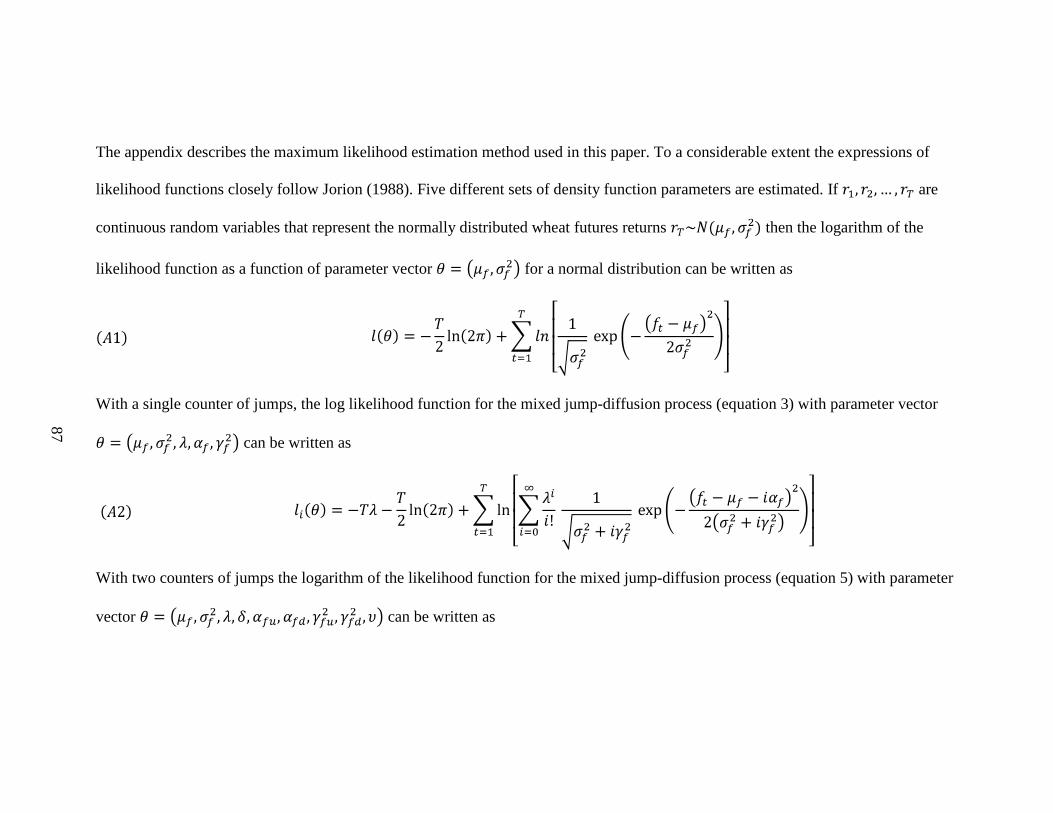
87
The appendix describes the maximum likelihood estimation method used in this paper. To a considerable extent the expressions of
likelihood functions closely follow Jorion (1988). Five different sets of density function parameters are estimated. If are
continuous random variables that represent the normally distributed wheat futures returns then the logarithm of the
likelihood function as a function of parameter vector for a normal distribution can be written as
With a single counter of jumps, the log likelihood function for the mixed jump-diffusion process (equation 3) with parameter vector
can be written as
With two counters of jumps the logarithm of the likelihood function for the mixed jump-diffusion process (equation 5) with parameter
vector can be written as
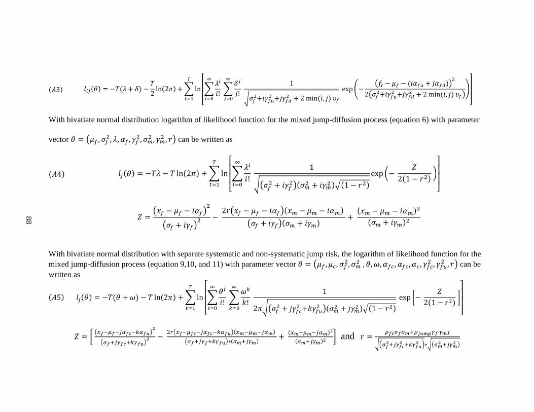
88
With bivatiate normal distribution logarithm of likelihood function for the mixed jump-diffusion process (equation 6) with parameter
vector can be written as
With bivatiate normal distribution with separate systematic and non-systematic jump risk, the logarithm of likelihood function for the mixed jump-diffusion process (equation 9,10, and 11) with parameter vector can be written as
and
VITA
Sijesh C. Aravindhakshan
Candidate for the Degree of
Doctor of Philosophy
Thesis: ESSAYS: BIOFUEL FEEDSTOCK PRODUCTION ECONOMICS AND IDENTIFYING JUMPS AND SYSTEMATIC RISK IN FUTURES
Major Field: Agricultural Economics Biographical:
Personal Data: Born in Thrissur, Kerala, India the son of Mrs. Thulasi Aravindhakshan and Mr. Aravindhakshan.
Education: Graduated with a Bachelors in Agriculture from Kerala Agricultural
University, India in March 2001; received a Master of Science degree in Agricultural Economics from Tamil Nadu Agricultural University, India, December 2003; received a Master of Science degree in Agribusiness and Applied Economics from North Dakota State University, December 2007; completed the requirements for the Doctor of Philosophy in Agricultural Economics at Oklahoma State University, July 2010.
Experience: Graduate Research Assistant, Oklahoma State University
Department of Agricultural Economics, January 2007 to May 2010; Graduate Research Assistant, North Dakota State University Department of Agribusiness and Applied Economics, August 2005 to December 2006; Agricultural Officer, Government of Kerala March 2003 to August 2005; Research Assistant, Communication Center, Kerala Agricultural University, June 2001 to December 2001.
Professional Memberships: Member, American Economic Association 2009 to
Present ; Member, Agricultural Economics Graduate Student Association 2007 to Present; Member, American Agricultural Economics Association 2008; Vice President, Kerala Gazetted Officers Association, Kerala, India 2003 to 2005; Secretary, Social Service League, College of Horticulture, Kerala, India 1997 to 2001