ESL Simulation Software - ISIM International Simulation ... 8.2.3 Development... · ESL Simulation...
210
ESL ESL Simulation Software Development Guide
Transcript of ESL Simulation Software - ISIM International Simulation ... 8.2.3 Development... · ESL Simulation...

ESL ESL
ESL
ESL Simulation Software Development Guide

ESL Simulation Software - Development Guide ii
Copyright ISIM International Simulation Limited 2018 – All Rights Reserved
Document Information
Version: 1.8. Date Published: February 2018.
This document relates to ESL version 8.2.3
ISIM welcomes any suggestions to improve the ESL Simulation Software and documentation
If you have any suggestions, or would like to point out any errors or omissions, please contact us:
ISIM International Simulation Limited
161 Claremont Road Salford M6 8PA UK
Tel: +44 (0) 161-736-5283 Fax: +44 (0) 087-1251-8549
Email: [email protected] Web: https://www.isimsimulation.com

Table of Contents
ESL Simulation Software - Development Guide iii
Table of Contents 1 Introduction .................................................................................................................... 1-1
1.1 The Integrated Simulation Environment (ISE) ...................................................... 1-1 1.2 The Simulation Language (ESL) .......................................................................... 1-1 1.3 Translator Options ................................................................................................ 1-2 1.3.1 Windows FORTRAN Compiler ......................................................................... 1-2 1.3.2 Windows C++ Compiler .................................................................................... 1-3 1.4 Document Conventions ........................................................................................ 1-3 1.5 User Liability ......................................................................................................... 1-3
2 Integrated Simulation Environment (ISE) .................................................................... 2-1 2.1 ISE Overview ........................................................................................................ 2-1 2.2 ISE Glossary ......................................................................................................... 2-2 2.2.1 Graphical Objects ............................................................................................. 2-2 2.2.2 Definitions ......................................................................................................... 2-2 2.3 ISE Interface ......................................................................................................... 2-2 2.3.1 The Message Area ............................................................................................ 2-2 2.3.2 The Canvas ....................................................................................................... 2-2 2.3.3 The Palette ........................................................................................................ 2-3 2.4 Working with Icons ............................................................................................... 2-3 2.4.1 Common Elements ........................................................................................... 2-3 2.4.2 Input/Output ...................................................................................................... 2-4 2.4.3 Library (Linear) .................................................................................................. 2-5 2.4.4 Library (Non-Linear) .......................................................................................... 2-6 2.4.5 Extra .................................................................................................................. 2-7 2.4.6 Instrumentation/Display Icons ........................................................................... 2-7 2.4.7 Annotation ......................................................................................................... 2-7 2.5 Working with Menus ............................................................................................. 2-8 2.5.1 File Menu .......................................................................................................... 2-8 2.5.2 Edit Menu .......................................................................................................... 2-8 2.5.3 View Menu ........................................................................................................ 2-9 2.5.4 Simulate Menu .................................................................................................. 2-9 2.5.5 Window Menu ................................................................................................... 2-9 2.5.6 Help Menu ....................................................................................................... 2-10 2.6 Working with Simulation Elements ..................................................................... 2-10 2.6.1 Simulation Element Short Cut Menu ............................................................... 2-10 2.6.2 Output Termination Short Cut Menu ............................................................... 2-11 2.6.3 Input Termination Short Cut Menu .................................................................. 2-11 2.6.4 Signal Line Shortcut Menu .............................................................................. 2-11 2.6.5 Signal Node Shortcut Menu ............................................................................ 2-11 2.6.6 Canvas Shortcut Menu ................................................................................... 2-11 2.6.7 Simulation Element Positioning ...................................................................... 2-11 2.6.8 Simulation Element Connecting ...................................................................... 2-12 2.6.9 Simulation Element Moving ............................................................................ 2-12 2.7 Parameters ......................................................................................................... 2-12 2.8 Package Manager .............................................................................................. 2-13 2.9 Attributes ............................................................................................................ 2-13 2.10 Working with Submodels .................................................................................... 2-14 2.10.1 Creating a Graphical Submodel ...................................................................... 2-15 2.10.2 Creating an Internal Textual Submodel .......................................................... 2-15 2.10.3 Choosing a Current Submodel ....................................................................... 2-16 2.10.4 Submodel Manager ......................................................................................... 2-16 2.11 Running a Simulation ......................................................................................... 2-17 2.11.1 Setup Window ................................................................................................. 2-17 2.11.2 Simulation Execution Window ........................................................................ 2-17 2.11.3 Control Panel Window .................................................................................... 2-18 2.11.4 Control Panel - Advanced Options ................................................................. 2-18

Table of Contents
ESL Simulation Software - Development Guide iv
2.11.5 Variables Window ........................................................................................... 2-19 2.11.6 Simulation Parameters Window ...................................................................... 2-19 2.12 Viewing Simulation Results ................................................................................ 2-19 2.12.1 Run Time Plot ................................................................................................. 2-20 2.12.2 Table ............................................................................................................... 2-20 2.12.3 Prepare ........................................................................................................... 2-21 2.12.4 Post Run Plot .................................................................................................. 2-21 2.13 The Toolbox ........................................................................................................ 2-21 2.13.1 Creating a Toolbox .......................................................................................... 2-22 2.13.2 Loading a Toolbox .......................................................................................... 2-22 2.13.3 Editing a Toolbox ............................................................................................ 2-23
3 ESL Basic Use ................................................................................................................ 3-1 3.1 ESL Suite of Programs ......................................................................................... 3-1 3.2 ESL Commands ................................................................................................... 3-2 3.2.1 Basic Commands .............................................................................................. 3-3 3.2.2 Command parameters ...................................................................................... 3-5 3.2.3 Files produced by ESL ...................................................................................... 3-6 3.2.4 File access ........................................................................................................ 3-6 3.2.5 Using ESL commands ...................................................................................... 3-7 3.2.6 Compiler and Interpreter ................................................................................... 3-7 3.2.7 Compiler and Translator ................................................................................... 3-9 3.2.8 User interaction ............................................................................................... 3-10 3.2.9 Post Run graphical analysis ........................................................................... 3-10 3.3 An ESL Program - Line-by-Line ......................................................................... 3-11 3.3.1 The program ................................................................................................... 3-11 3.3.2 Lexical components ........................................................................................ 3-13 3.3.3 Comments ....................................................................................................... 3-14 3.3.4 Include files ..................................................................................................... 3-14 3.3.5 Program structure and modules ..................................................................... 3-15 3.3.6 PACKAGE definition ....................................................................................... 3-16 3.3.7 Reserved PACKAGE ...................................................................................... 3-17 3.3.8 Run specification ............................................................................................. 3-17 3.3.9 Integration selection ........................................................................................ 3-18 3.3.10 Model definition ............................................................................................... 3-19 3.3.11 Results from the ESL example ....................................................................... 3-27
4 ESL Operation and Program Structure ........................................................................ 4-1 4.1 ESL Program Types ............................................................................................. 4-1 4.1.1 The ESL STUDY ............................................................................................... 4-1 4.1.2 The ESL REMOTE program ............................................................................. 4-2 4.1.3 The ESL EMBEDDED program ........................................................................ 4-2 4.1.4 The ESL non program....................................................................................... 4-3 4.2 ESL Program Structures....................................................................................... 4-3 4.2.1 ESL data types .................................................................................................. 4-3 4.2.2 The ESL experiment ......................................................................................... 4-4 4.2.3 The ESL MODEL .............................................................................................. 4-4 4.2.4 The ESL SUBMODEL ....................................................................................... 4-5 4.2.5 The ESL SEGMENT ......................................................................................... 4-6 4.2.6 The ESL PROCEDURE .................................................................................... 4-7 4.2.7 The ESL PACKAGE .......................................................................................... 4-7 4.3 Procedural Subprogram Structure ........................................................................ 4-8 4.4 Modelling Subprogram Structure ........................................................................ 4-10 4.4.1 Modelling code ................................................................................................ 4-10 4.4.2 Procedural code .............................................................................................. 4-10 4.4.3 Modelling subprogram regions ....................................................................... 4-11 4.5 Variables - scope, type and usage ..................................................................... 4-13 4.5.1 Model parameters ........................................................................................... 4-13 4.5.2 State variables ................................................................................................ 4-15 4.5.3 Algebraic variables .......................................................................................... 4-17

Table of Contents
ESL Simulation Software - Development Guide v
4.5.4 Procedural variables ....................................................................................... 4-17 4.5.5 CONSTANTS .................................................................................................. 4-18 4.5.6 ESL PARAMETERS ....................................................................................... 4-18 4.6 The Simulation Process...................................................................................... 4-19 4.6.1 The model functions ........................................................................................ 4-19 4.6.2 Sorting modelling code ................................................................................... 4-20 4.6.3 Submodel data store ....................................................................................... 4-22 4.6.4 Initialisation sequence..................................................................................... 4-22 4.6.5 COMMUNICATION code ................................................................................ 4-24 4.6.6 STEP code ...................................................................................................... 4-24
5 Modelling Code .............................................................................................................. 5-1 5.1 Differential Equations ........................................................................................... 5-1 5.1.1 Prime notation ................................................................................................... 5-1 5.1.2 Integral notation ................................................................................................ 5-2 5.1.3 Submodel representation .................................................................................. 5-2 5.1.4 Laplace transform notation ............................................................................... 5-3 5.2 Integration Methods .............................................................................................. 5-6 5.2.1 Basis of numerical integration ........................................................................... 5-6 5.2.2 ESL integration algorithms ................................................................................ 5-9 5.3 Discontinuities .................................................................................................... 5-15 5.3.1 ESL handling of discontinuities ....................................................................... 5-15 5.3.2 ESL action on discontinuity detection ............................................................. 5-17 5.3.3 Logical assignment of discontinuity ................................................................ 5-18 5.4 Partial Differential Equations .............................................................................. 5-24 5.4.1 Electrical transmission line ............................................................................. 5-25 5.4.2 Heat flow or diffusion ...................................................................................... 5-26 5.4.3 Simulating partial differential equations .......................................................... 5-27
6 Arrays, Matrices, Vectors and Characters .................................................................. 6-1 6.1 Array Declarations ................................................................................................ 6-1 6.1.1 Subprogram array arguments ........................................................................... 6-2 6.1.2 Vector declarations ........................................................................................... 6-3 6.1.3 Dynamic arrays ................................................................................................. 6-3 6.1.4 Array initialisation .............................................................................................. 6-3 6.1.5 Printing arrays ................................................................................................... 6-4 6.2 Array Subscripts ................................................................................................... 6-6 6.3 Array Slicing ......................................................................................................... 6-6 6.4 Array Operations .................................................................................................. 6-8 6.4.1 Array assignment .............................................................................................. 6-8 6.4.2 Character assignment ....................................................................................... 6-9 6.4.3 Interrogating array sizes ................................................................................... 6-9 6.4.4 Numerical array (matrix) operations ................................................................. 6-9 6.4.5 Vector operations ............................................................................................ 6-10 6.4.6 Array functions ................................................................................................ 6-11 6.5 Character Array Operations ............................................................................... 6-12 6.5.1 Character array functions ............................................................................... 6-12 6.5.2 Character comparison..................................................................................... 6-13 6.5.3 Characters as subprogram arguments ........................................................... 6-13 6.5.4 Character function procedures ....................................................................... 6-13
7 Multivariable Transfer Functions ................................................................................. 7-1 7.1 Introduction ........................................................................................................... 7-1 7.2 Example 1 - Multivariable feedback control system ............................................. 7-2 7.3 Example 2 - Coupled two-mass system ............................................................... 7-4 7.4 Limitations ............................................................................................................ 7-6
8 Input-Output and File Handling .................................................................................... 8-1 8.1 Connecting Files ................................................................................................... 8-1 8.1.1 Opening, creating and rewriting files ................................................................ 8-1

Table of Contents
ESL Simulation Software - Development Guide vi
8.1.2 Closing file connections .................................................................................... 8-2 8.2 File Deletion .......................................................................................................... 8-3 8.3 Input/Output Error Status...................................................................................... 8-3 8.4 The PRINT Statement .......................................................................................... 8-4 8.4.1 Data output formatting ...................................................................................... 8-6 8.5 The TABULATE Statement .................................................................................. 8-7 8.6 The READ Statement ........................................................................................... 8-8 8.6.1 Free format input ............................................................................................... 8-8 8.6.2 Keyboard input .................................................................................................. 8-9 8.6.3 The READEL statement.................................................................................. 8-10 8.6.4 Data input formatting....................................................................................... 8-11 8.6.5 READ examples .............................................................................................. 8-12 8.7 The PREPARE Statement .................................................................................. 8-13 8.8 The PLOT Statement .......................................................................................... 8-14 8.9 The CLEAR_SCREEN statement ...................................................................... 8-14 8.10 The convertDisplayFile program ........................................................................ 8-14
9 ESL Segments ................................................................................................................ 9-1 9.1 Introduction ........................................................................................................... 9-1 9.2 Emulated Segment Operation .............................................................................. 9-2 9.2.1 The multi-processor concept ............................................................................ 9-2 9.2.2 Emulated segment ............................................................................................ 9-3 9.2.3 Basic segment programming ............................................................................ 9-4 9.3 Distributed Simulation Execution .......................................................................... 9-7 9.4 Embedded Segments ......................................................................................... 9-13 9.4.1 Embedded simulation using FORTRAN ......................................................... 9-13 9.4.2 Embedded simulation using C++ .................................................................... 9-18 9.5 Generation of Interface Modules for Embedded Segments ............................... 9-22 9.5.1 Using the '-dll' option in a C (or C++) application: .......................................... 9-25 9.5.2 Using the '-com' option in a C++ application:.................................................. 9-26 9.5.3 Using the '-clr' option in a C# application: ....................................................... 9-26
10 Steady-State Analysis ............................................................................................. 10-1 10.1 Introduction ......................................................................................................... 10-1 10.2 The ANALYSIS Region ...................................................................................... 10-2 10.3 The TRIM Statement .......................................................................................... 10-2 10.4 The LINEARIZE Statement ................................................................................ 10-3 10.5 The EIGENVALUE Statement ............................................................................ 10-4 10.6 The ANALYSIS MODEL Call .............................................................................. 10-4 10.7 Steady-State Algorithms ..................................................................................... 10-5 10.8 Optimization ........................................................................................................ 10-6 10.9 Two Link Robot Arm Example ............................................................................ 10-7
11 ESL Run Control ...................................................................................................... 11-1 11.1 INTERACT Control ............................................................................................. 11-1 11.2 Simulation Driver Files........................................................................................ 11-4 11.3 RESUME and RESTART ................................................................................... 11-6 11.4 Snapshot Support ............................................................................................... 11-6
12 External Procedures ................................................................................................ 12-1 12.1 Introduction ......................................................................................................... 12-1 12.2 External FORTRAN and C Routines .................................................................. 12-1 12.3 External C++ Routines ....................................................................................... 12-9
Chapter 1 Introduction
ESL Simulation Software - Development Guide 1-1
CHAPTER 1
1 Introduction Welcome to ESL.
ESL is a powerful and flexible software package used to simulate complex dynamic systems. It comprises the simulation language itself (ESL) and its graphical user interface - Integrated Simulation Environment (ISE).
If you have the ESL-CORE component only, and not the full system, then the graphical Integrated Simulation Environment (ISE) described in this help documentation is not available. ESL applications can only be developed textually.
1.1 The Integrated Simulation Environment (ISE)
ISE provides the following facilities:
Multi-window graphical block diagram editor for model construction.
Inclusion of ESL coded submodels where appropriate.
Interactive control of simulation execution.
Run-time and post-run graph plotting.
User configurable simulation element palette.
Application specific toolbox capability.
Display manager.
Local help.
ISE is the development environment from which you can manage each stage of the simulation activity. ISE includes a graphical editor for block diagram style model descriptions, while allowing textual ESL code to be used where appropriate (for example, to describe highly non-linear elements). You select standard simulation elements from a palette and interconnect them on a canvas to build up the simulation description. ESL submodels can be created and included in a diagram through a special submodel element. You have the option to configure the simulation element palette itself with user defined submodels and thus create your own application specific toolboxes.
Once you have created a simulation program (graphically, textually or a combination of both), compilation is initiated from ISE. You then have the option to execute the compiled program immediately through an interpreter, or further translate it to C++ or FORTRAN. The resulting executable program may then be run from ISE. In either case, execution is managed by an interactive control panel which provides run-time control of the simulation. You have access to all program variables and parameters from the control panel. This includes simulation parameters such as the communication interval, final simulation time, choice of integration algorithm and error tolerances. All variables and parameters can be set and changed dynamically from the control panel. You can specify graphical and tabulated output on your block diagram through the use of special simulation display elements or alternatively from a versatile display manager window. You can log all run time commands and output specifications to a driver file that can be used at a later time to repeat simulation scenarios.
1.2 The Simulation Language (ESL) ESL was written to meet the simulation requirements of the European Space Agency. It is a general purpose Continuous System Simulation Language (CSSL) with discrete event capabilities and may be applied in any field where dynamic systems are to be studied.

Chapter 1 Introduction
ESL Simulation Software - Development Guide 1-2
The main characteristics of ESL are:
Provision of an Interpreter for fast program development, and a Translator (providing C++ or FORTRAN code) for efficient production runs.
A well-defined lexical structure.
Separate program units may be used to describe the system and the experiment to be performed on it.
Modular model concepts in the form of submodels to define independent parts of the system within a hierarchical structure.
Parallel processor segmentation concepts to enable models to be partitioned into segments and executed concurrently in a multiple-processor environment.
Techniques for the accurate description and detection of discontinuities.
Steady-state finding and linearization facilities.
Full matrix/vector operations.
Derivative notation, integral notation and transfer-function notation for describing differential equations.
Comprehensive run-time and post-run graphical display of results.
Automatic ordering of the model definition equations.
Eight numerical integration algorithms including three stiff methods.
Extensive diagnostic checks during compilation to determine model "correctness".
C++, C or FORTRAN routines may be incorporated into a simulation that has been created through the translator route.
ESL segments may be run embedded in a non-ESL C++ or FORTRTAN main program.
Facilities to dynamically communicate with other program modules via FORTRAN common blocks or C++ structures.
Full range of standard procedural facilities including file and character handling.
Extensive library of ESL submodels which may be incorporated into user programs.
1.3 Translator Options To use ESL in translator mode, it is necessary to have installed an appropriate FORTRAN and/or C++ compiler. Both of the options given below for Windows are or have public domain versions.
Note that the translator mode and associated features (such as calling external routines and embedded ESL simulations), are not available if you only have ESL-Lite installed.
1.3.1 Windows FORTRAN Compiler
For FORTRAN translation, you should install the MinGW FORTRAN compiler.
This is available in the MinGW - Minimalist GNU for Windows software package - see http://www.mingw.org/.
From the downloads page (https://sourceforge.net/projects/mingw/files/) you should download the mingw-get-setup.exe (version 0.6.2-beta-20131004-1 or above) (https://sourceforge.net/projects/mingw/files/latest/download?source=files).
We recommend that you open the setup file as an Administrator and select to install it for all users on the default path (C:\MinGW).
Chapter 1 Introduction
ESL Simulation Software - Development Guide 1-3
It will open an installer window that allows you to select packages for installation and then apply those changes which will download and install the components for those packages.
For FORTRAN translation you should install the mingw32-base and mingw32-gcc-fortran packages (but see below for also selecting the mingw32-gcc-g++ to support C++).
1.3.2 Windows C++ Compiler
For C++ translation, you have the option of:
1. Microsoft Visual Studio C++ compiler (2008 or above): http://www.visualstudio.com/. The freely available Visual Studio Express versions are perfectly adequate. This is the compiler that will be used by default.
2. MinGW C++ compiler: http://www.mingw.org/. You should install the mingw32-base and mingw32-gcc-g++ packages. See 1.3.1 above for more details on installing this software package.
To use this compiler you need to set the ESLCCOMP environment variable to GCC.
1.4 Document Conventions Certain typographical conventions are used to emphasise special text in the documentation.
ESL code, computer output, user commands and responses are shown in a different style, for example:
sample of font used for ESL code.
A bold font if often used to denote ESL keywords and program variables, for example MODEL.
To help explain some user interactions the symbol is used to represent an "Enter" or "Return" key press, for example:
esl rocket
1.5 User Liability A properly conducted simulation study can make a valuable contribution to decision making processes. On the other hand, an improperly conducted study can give misleading information which may lead to an inappropriate decision and extremely expensive consequences.
It is the user's responsibility to conduct a simulation study in a proper manner, and to perform tests that confirm simulation results are acceptable in the context on any particular decision.
Simulation software tools such as ESL, or in fact any tool, even a garden spade, can be used correctly to produce desired results, or used incorrectly with disastrous results
A simulation study comprises the following phases:
Derivation of mathematical model of dynamic system.
Conversion and verification of mathematical model as ESL program.
Simulation execution.
Validation and analysis of simulation results.
Errors can be introduced during any of the above phases. The mathematical model must adequately represent the system in order to be able to satisfy the objects of the study. The ESL program should correspond to the mathematical model exactly, and the simulation execution must not introduce unacceptably large errors. You will appreciate, perhaps, how errors may be introduced during the first two phases of a simulation. The origin of errors introduced during simulation execution is less clear, and needs some explanation.

Chapter 1 Introduction
ESL Simulation Software - Development Guide 1-4
The heart of a simulation is the numerical integration process. The very nature of numerical integration is such that it produces results which are defined as an "approximate" solution to differential equations. It is the user's responsibility to ensure that results are within acceptable limits. This means that the integration should always be operating within its stability bounds, and the truncation, round-off and global errors should always be within acceptable limits. Basically this means the selection of an appropriate integration algorithm, and step-length control parameters. Variable-step integration attempts to achieve these requirements, but is not fool proof - there will always be problems that confound it. At best such methods give a good first approximation to the correct step-length, and it is the user's responsibility to confirm that this approximation is acceptable. For example, a useful process with fixed-step explicit integration is to repeat a simulation with a step-length half that of the first simulation attempt. Only if the results are sufficiently close should the original step-length be regarded as acceptable.
Even when the integration is working properly some dynamic systems can cause erratic simulation behaviour because the real system is itself highly unstable, and the simulation represents this instability. In these cases the slightest integration error, or in fact any small perturbation, can be magnified and lead to a gross error. Consider a circus acrobat balancing on a ball on a tightrope. This is highly unstable as the smallest error by the acrobat could cause a fall. The simulation of such a system could introduce a small simulation error which would have the same effect as an error by the acrobat that is a fall. In this case it is the simulation that introduced the error and was the cause of the fall.
Two words "verification" and "validation" are used to describe processes in a proper simulation study which help to ensure the integrity of the results.
The "verification" process is used to ensure that the simulation results sufficiently accurately represent the behaviour of the mathematical model (not the dynamic system).
The "validation" process is used to ensure that the simulation results sufficiently accurately represent the behaviour of the real dynamic system.
Verification of a simulation study has the restricted objective of ensuring the integrity of the solution of the mathematical model. This includes: confirmation that results obtained from mathematical analysis of the model can be produced by simulation; that the numerical integration is giving stable answers within acceptable error bounds; and tests to confirm the behaviour of the simulation actually reflects that expected from the mathematical model.
Validation of a simulation study has the overall objective of ensuring that the simulation results sufficiently accurately represent the behaviour of the dynamic system. This is achieved by comparing simulated results with known, or predicted, performance of the dynamic system, and where possible, comparing real system data to the simulated results. This process must confirm the mathematical model adequately represents the system, and also perform the processes described as verification.
Even following the above processes problems can occur. For example, the simulated system may encounter a situation which has not been the subject of a specific validation test, possibly because little or no information is available about this particular situation. In such cases great care must be exercised in the interpretation of any results.
In this section we have emphasised the problems which may be encountered, and the rigorous procedures which must be followed if decisions are to be made based on results of simulation. In conclusion, it should be noted that ESL probably provides a better environment than any comparable software for helping the user to perform a validated simulation study.

Chapter 2 Integrated Simulation Environment (ISE)
ESL Simulation Software - Development Guide 2-1
CHAPTER 2
2 Integrated Simulation Environment (ISE)
The section describes the Integrated Simulation Environment (ISE).
Contents:
ISE Overview
ISE Glossary
ISE Interface
Working with Icons
Working with Menus
Working with Simulation Elements
Parameters
Attributes
Working with Submodels
Running a Simulation
Viewing Simulation Results (Run Time Plot, Table, Prepare, Post Run Plot)
The Toolbox
2.1 ISE Overview The Integrated Simulation Environment (ISE) provides you with an interface to develop dynamic simulation models using graphical editing of 'block diagrams'. These block diagrams are then translated into European Simulation Language (ESL) programs and executed from ISE.
The user palette provides a Standard Toolbox in which sets of icons represent such elements as linear, arithmetic, and logical operators, standard functions, and submodels.
You define attributes and parameters for each element, and, by graphically connecting elements, represent required simulations. Once defined, you can assign icons to a submodel and add them to a custom toolbox.
You can also create textual submodels by writing ESL code in a text editor.
Attributes and parameters, together with simulation runs, are controlled through a combination of menus and dialog boxes.
You can run simulations from ISE and view the results in graph plot or table form. Result plots and tables, as well as simulation diagrams, may be printed or saved to disk.
When active, ISE may be in one of two modes of operation:
Edit - simulation not running, graphical/text editing of the application can take place.
Run - simulation running, graphical editing/opening a new text edit window disabled (graphical display may still be defined).

Chapter 2 Integrated Simulation Environment (ISE)
ESL Simulation Software - Development Guide 2-2
2.2 ISE Glossary
2.2.1 Graphical Objects
Simulation element - a single functional block appearing on an ESL block diagram. The simulation element appears when you drag an icon from the palette onto the canvas. Most simulation elements have a fixed number of inputs and outputs.
Instrumentation/Display icons - indicate a monitoring or output operation. There are two icons: Table and Plot.
Instrumentation display - actual plot or table associated with instrumentation/display icon.
Termination - input or output connection to a simulation element.
Signal line - interconnection between simulation element terminations.
Signal line node - appears at bends and interconnections of signal lines.
Instrumentation lines - connection from a signal line, signal line node, or termination to an instrumentation /display icon.
Annotation objects - descriptive text.
2.2.2 Definitions
Application - a single complete ISE simulation (held in a file with a .ise extension).
Compilation - unless qualified by FORTRAN or C++, refers to conversion of ESL source text into intermediate (hcd) code.
Translation - conversion of hcd into FORTRAN or C++ by ESL translator program.
Interpretation - direct execution of hcd by ESL interpreter program.
Execution - running executable program created by FORTRAN or C++ compilation of the translator output linked with the run-time library (and, optionally, user code/libraries).
2.3 ISE Interface The ISE interface consists of three main elements: the message area, the canvas, and the palette.
2.3.1 The Message Area
ISE uses the message area to inform you of current processes, errors, and information regarding the active simulation. The size of the message area can be changed by dragging the divider bar between it and the canvas up or down.
2.3.2 The Canvas
The canvas is the main workspace in the ISE environment. You drag icons from the palette onto the canvas, where they may be moved, manipulated, configured, or connected to other simulation elements. The canvas is provided with a grid to which simulation elements snap when dragged. Grid size and snap-to attributes, as well as canvas background colour, are user-definable.

Chapter 2 Integrated Simulation Environment (ISE)
ESL Simulation Software - Development Guide 2-3
2.3.3 The Palette
The palette may be considered the storage area for simulation elements. Each element, whether a simple arithmetic operator such as a summer or a complicated user-defined simulation submodel, can be saved as an icon in a panel of a toolbox. Each panel is further divided into a series of areas. You select one of the panels from a drop-down list in the palette itself, and then use the required element by dragging its icon from the palette onto the canvas.
2.4 Working with Icons In the Standard Toolbox, the palette is divided into five panels of icons:
Common Elements
Input/Output
Library (Linear)
Library (Non-Linear)
Extra
The icons are listed below. Where the placing of an icon results in the generation of a call to an ESL library submodel or procedure: the name of the library item is provided. A full list of library submodels and procedures will be found in the ESL Reference Manual.
2.4.1 Common Elements
The Common Elements panel of the Standard Toolbox is divided into the following areas and elements, each of which is shown with a representation of its specific icon:
Linear Operators
Transfer Function
Constant Multiplier
Integrator
Arithmetic Operators
Summer
Summer3
Multiplier
Divider
Logical Operators
Logical Negation
Logical And
Logical Or

Chapter 2 Integrated Simulation Environment (ISE)
ESL Simulation Software - Development Guide 2-4
Standard Functions
Sine
Cosine
Tangent
Absolute submodel ABSX
Arcsine
Arccosine
Arctangent
Arctangent2
Exponential
Natural Logarithm
Base 10 Logarithm
Raise x to power y
Square Root procedure SQRTX
Integer submodel INTX
2.4.2 Input/Output
The Input/Output panel of the Standard Toolbox is divided into the following areas and elements:
Inputs
Step Input submodel STEPP (used with additional ESL code)
Sinusoidal
Ramp Input submodel RAMP
Square Input submodel MODULT (used with additional ESL code)
Time Input
Impulse submodel IMPUL
Constant Real
Constant Integer

Chapter 2 Integrated Simulation Environment (ISE)
ESL Simulation Software - Development Guide 2-5
Logical True
Logical False
Logical Constant
Input Arguments
Real Input
Integer Input
Logical Input
Output Arguments
Real Output
Integer Output
Logical Output
2.4.3 Library (Linear)
The Library (Linear) panel of the Standard Toolbox is divided into the following areas and elements (which correspond to the linear ESL library submodels stored in ESL's lib directory):
Laplace Operators
Second Order System submodel CMPXPL
Lead-lag submodel LEDLAG
First Order System submodel REALPL
Integrators
Fourier Transform submodel FOURINT
Standard Integrator
Limited Integrator submodel LIMINT
Logical Integrator submodel LOGINT
Controllers
PI Control submodel PICONT
PID Control submodel PIDCONT
Advanced PID Control submodel PIDCONT1

Chapter 2 Integrated Simulation Environment (ISE)
ESL Simulation Software - Development Guide 2-6
Timers
Timer submodel TIMER
2.4.4 Library (Non-Linear)
The Library (Non-Linear) panel of the Standard Toolbox is divided into the following areas and elements (which correspond to the non-linear ESL library submodels stored in ESL's lib directory):
Oscillators
Bistable submodel BISTBL
Modulator submodel MODULT
Monostable submodel MONO
Comparators
Comparator
Backlash submodel COMPB
Digitisers
Delay submodel DELAY
Derivative submodel DERIV
First Order Hold submodel FHOLD
Quantizer submodel QNTZR
Sample and Hold submodel SAMHLD
Zero Order Hold submodel ZHOLD
Limiters
Deadspace submodel DEADSP
Hysteresis submodel HSTRSS
Limiter submodel LIMIT
Misc
Rectifier submodel RECT
Friction submodel COULOMB
Switch

Chapter 2 Integrated Simulation Environment (ISE)
ESL Simulation Software - Development Guide 2-7
2.4.5 Extra
The Extra panel of the Standard Toolbox is divided into the following areas and elements:
Function Generator
Function Generator procedure FG3D
Submodel
Submodel
Annotation
Annotation
Display Icons
Plot
Table
2.4.6 Instrumentation/Display Icons
Plot
Table
These icons provide an intuitive method to let you set display options for selected variables.
Drag a Plot or Table icon from the palette onto the canvas.
Right click the icon to invoke the shortcut menu.
Select Connect: an instrumentation (dotted) line is produced and is linked to a signal line, node, or termination by left-clicking. Connect mode is still active to allow further connections to be made until closed by a right click. Multiple connections to the same signal line are not allowed. Instrumentation lines may not be selected, but may be deleted by right-clicking and selecting Disconnect.
Select Properties from the shortcut menu: the Table/Plot Properties dialog is opened to allow default settings to be altered.
Select Display from the shortcut menu or double-click the icon. The display window opens with default/specified properties. In the case of the Plot icon: if there is a simulation running, a plot window with a default axis is opened, and axes limits automatically adjust as the run continues. If no simulation is running, a plot window is opened and a graph from an associated prepare file is displayed. If no such prepare file exists, an error message is generated. Note that prepare files are automatically generated for instrumentation/display icons. A default name, which may be changed in the appropriate window, is used as a basis for the prepare file name.
2.4.7 Annotation
Annotation icon
Drag the icon from the palette onto the canvas. You may enter any descriptive text and subsequently move it.

Chapter 2 Integrated Simulation Environment (ISE)
ESL Simulation Software - Development Guide 2-8
2.5 Working with Menus The following menus are available from the ISE main window:
File Menu
Edit Menu
View Menu
Simulate Menu
Window Menu
Help Menu
2.5.1 File Menu
New - allows you to open a new workspace. Note that ISE only allows one simulation application to be open at any one time. If the New command is selected while work is active, you will be prompted to save your work. If you choose not to save that work, a new workspace will be opened and old work lost.
Open - opens an existing application. The note above about only one simulation open at any one time applies.
Save - allows you to save the changes made to the simulation application since the last Save.
Save As - allows you to save a simulation application for the first time, or to save an existing application under an alternative name.
Print - brings up the dialog box to print a simulation model, or the results of a simulation run. Only prints the visible area of the canvas.
Editor - invokes a user-specified text editor; you may edit ESL code, text, and FORTRAN/C++ code.
Display Conversion - allows you to select a display file, either a prepare ('.dsp') or tabulate ('.tab') file, and convert it to the other file format.
Exit - quits ISE.
2.5.2 Edit Menu
Certain of the Edit operations (Cut, Copy, Delete, Flip and Rotate) act on selected simulation elements. Simulation elements are selected with a left mouse button click. Multiple elements can be selected by holding down the Ctrl key while clicking or by extending a selection box around the elements. (Position the pointer on the canvas, hold down the left mouse button, extend the rectangular selection box over the elements and release the button. If you attempt to extend the rectangle beyond the limits of the canvas, the window will scroll appropriately).
Undo (Ctrl+Z) - allows you to 'undo' the effects of the last change made. You can undo back as far as the last Save.
Redo (Ctrl+Y) - allows you to 'redo' a change which has been 'undone'.
Cut (Ctrl+X) - copies a selected element to the clipboard and removes it from the canvas.
Copy (Ctrl+C) - copies a selected element to the clipboard (copied element remains on the canvas).
Paste (Ctrl+V) - pastes the contents of the clipboard onto the canvas.
Delete (Del) - deletes selected elements.

Chapter 2 Integrated Simulation Environment (ISE)
ESL Simulation Software - Development Guide 2-9
Flip - Left/Right: reflects the selected element about the vertical axis; Up/Down: reflects the selected element about the horizontal axis.
Rotate - rotates the selected element by 90 degrees either left or right. Flip/Rotate is used either to change the orientation of a selected element or to swap the positions of input/output terminations.
Use Packages - allows you to make ESL packages accessible in the current module. See Packages and Package Manager.
Parameters - allows the definition, deletion, or modification of parameters for use as simulation element attributes. See Parameters.
Edit Experiment - opens the text editor and allows you to enter/modify the experiment for an ESL MODEL.
Reset Experiment - resets the experiment to default generated value. This may be useful if you changed any Input/Output parameter entities in the model since previously editing it.
Simulation Parameters - allows you to set the simulation parameters that define the basic properties of the simulation to be run. The simulation parameters can be changed dynamically at run-time (see Simulation Parameters Window).
Properties - allows you to set the property of the current window diagram to determine how the ESL code is generated. If it is the main window, its property can be set to Model, Embedded Segment or Remote Segment; if it is a submodel window, its property can be set to Submodel or External Segment. See ESL Segments for a complete discussion of segments.
2.5.3 View Menu
Toolbar - toggles toolbar (visible/hidden).
Zoom - invokes a canvas Zoom Factor dialog, in which the zoom factor may be set as a percentage.
Zoom Reset - resets the canvas zoom factor to 100%.
Zoom All - sets zoom factor to show all elements on canvas.
Customise - allows the main window or submodel window toolbars to be customised.
Options - opens the options dialog from which you can alter the appearance of the canvas, palette, simulation elements and connections.
Load Options - allows you to load an options file. Examples of options files (with .opt extension) are provided in the ise\examples directory.
Save Options - allows you to save the current options to a file.
2.5.4 Simulate Menu
Run - initiates a simulation run. This generates the ESL code for the current application and compiles and runs it. See Running a Simulation.
Setup - invokes the Simulation Setup dialog box allowing simulation options to be set. See Running a Simulation.
Build Only - builds but does not run the current application. Used particularly when creating Embedded, Remote or External Segments. See Running a Simulation.
2.5.5 Window Menu
Simulation Execution - allows you to run an external ESL program. You can specify a source file (usually an '.esl' source, '.hcd' compiled or an executable). There is a corresponding range of Execution Command options that may be specified. This

Chapter 2 Integrated Simulation Environment (ISE)
ESL Simulation Software - Development Guide 2-10
facility will not be available if the Control Panel Window is displayed, since only one simulation may be running at any one time.
Display Manager - allows you to configure plots and tables for displaying the results of simulation runs. Each plot/table can display output from one or several application variables. See Viewing Simulation Results.
Submodel Manager - allows the management of all submodels in an application. See Working with Submodels.
Package Manager - allows the creation and editing of packages within an application.
2.5.6 Help Menu
Contents - on-line user documentation for ESL and ISE.
About ESL - displays the software version and copyright information.
2.6 Working with Simulation Elements The following steps outline the process of creating a simulation diagram:
Drag icons from the palette to the canvas where they appear as simulation elements. Alternatively, select a simulation element from the canvas shortcut Insert menus.
Connect simulation element terminations by signal lines.
Specify simulation element attributes.
Apply graphical editing operations such as move, cut, copy, paste, and delete.
Drag instrumentation/display icons from the palette to the canvas.
Connect instrumentation/display icons to an arbitrary number of signal lines by instrumentation lines.
Add free annotation text to the diagram.
2.6.1 Simulation Element Short Cut Menu
Each simulation element has a shortcut (or context) menu which is accessed by right-clicking the element.
The shortcut menu includes commands from the Edit menu: Cut, Copy, Delete, Flip, and Rotate. The Attributes dialog box may also be invoked from the shortcut menu.
In addition, those simulation elements that invoke standard ESL library submodels (most of the Linear and Non-linear Library elements) include a View Lib... option, which opens the text editor to view the submodel file.
Where a Help URL has been specified in the toolbox (as a file or URL), the shortcut menu has a Help... command, which will open the file or URL in the default application (e.g. text editor or browser).
Submodel shortcut menus include additional options:
Set Definition - allows the creation of a new submodel or the viewing and selection of current definitions.
Edit - (for internal submodels) opens the Submodel graphical window or the text editor for editing.
View - (for external submodels) opens the text editor to view the submodel file.

Chapter 2 Integrated Simulation Environment (ISE)
ESL Simulation Software - Development Guide 2-11
Update Definition - allows the element to be refreshed if the definition has been changed.
Attributes... - allows a name to be specified for the submodel instance.
2.6.2 Output Termination Short Cut Menu
Right-clicking a simulation element's output termination invokes a shortcut menu with a single Output Attributes... option. Selecting Output Attributes... opens an Output Variable dialog enabling you to attach a user-defined name. This name then becomes the name of the corresponding output variable.
The Output Variable dialog has a Name text entry field which contains a default name which would, normally, be changed to reflect the actual output. If the box to the left of Name is checked, the name appears as an annotation on the diagram. If the box to the left of Attributable is checked the output may be assigned to a simulation element attribute. See Attributes.
The displayed annotation may be moved relative to the simulation element by dragging.
2.6.3 Input Termination Short Cut Menu
The Input Terminations of arithmetic simulation elements display a sign. The default is a "+" and a "-" for a two-input summer, both "+" for multipliers and dividers. Right-clicking any of these input terminations invokes a shortcut menu with a single Toggle Sign option.
2.6.4 Signal Line Shortcut Menu
Right-clicking a signal line invokes the appropriate shortcut menu:
Delete Line - deletes the line segment and all connected line segments and nodes back to a simulation element termination, or to a node which connects three or more elements.
Disconnect - deletes the line segment only.
Insert Node - inserts a node into the line segment (for example, to bend a line segment by moving the node).
2.6.5 Signal Node Shortcut Menu
Right-clicking a signal node invokes the appropriate shortcut menu:
Delete Line - deletes the node and all connected line segments and nodes back to a simulation element termination or a node connecting three or more line segments.
Disconnect - deletes the node and immediate line segment only.
Delete Node - deletes the node and immediate line segments, and will reconnect to maintain signal flow. This reconnection only happens if one connected line segment can be traced back to a simulation element output termination, such as a signal flow into the node. Otherwise it operates like Delete Line above.
2.6.6 Canvas Shortcut Menu
Includes Undo, Redo, Cut, Copy, Paste, Delete, Flip, Rotate, Use Package, Parameters and Properties from the Edit Menu plus:
Insert - allows you to select and insert simulation elements. The element is inserted at the position on the canvas where the shortcut menu was opened.
2.6.7 Simulation Element Positioning
You move icons from the palette to the canvas by 'dragging and dropping' with the left mouse button. Elements may not be dragged directly from the palette on top of another element.
Chapter 2 Integrated Simulation Environment (ISE)
ESL Simulation Software - Development Guide 2-12
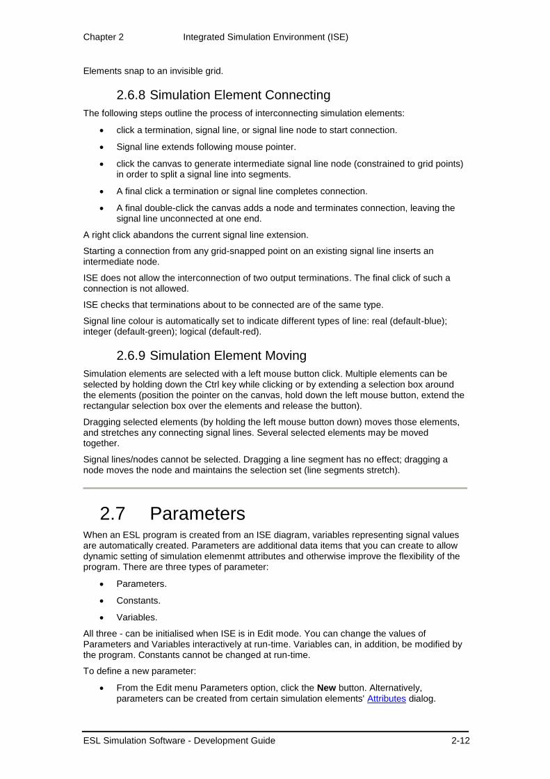
Elements snap to an invisible grid.
2.6.8 Simulation Element Connecting
The following steps outline the process of interconnecting simulation elements:
click a termination, signal line, or signal line node to start connection.
Signal line extends following mouse pointer.
click the canvas to generate intermediate signal line node (constrained to grid points) in order to split a signal line into segments.
A final click a termination or signal line completes connection.
A final double-click the canvas adds a node and terminates connection, leaving the signal line unconnected at one end.
A right click abandons the current signal line extension.
Starting a connection from any grid-snapped point on an existing signal line inserts an intermediate node.
ISE does not allow the interconnection of two output terminations. The final click of such a connection is not allowed.
ISE checks that terminations about to be connected are of the same type.
Signal line colour is automatically set to indicate different types of line: real (default-blue); integer (default-green); logical (default-red).
2.6.9 Simulation Element Moving
Simulation elements are selected with a left mouse button click. Multiple elements can be selected by holding down the Ctrl key while clicking or by extending a selection box around the elements (position the pointer on the canvas, hold down the left mouse button, extend the rectangular selection box over the elements and release the button).
Dragging selected elements (by holding the left mouse button down) moves those elements, and stretches any connecting signal lines. Several selected elements may be moved together.
Signal lines/nodes cannot be selected. Dragging a line segment has no effect; dragging a node moves the node and maintains the selection set (line segments stretch).
2.7 Parameters When an ESL program is created from an ISE diagram, variables representing signal values are automatically created. Parameters are additional data items that you can create to allow dynamic setting of simulation elemenmt attributes and otherwise improve the flexibility of the program. There are three types of parameter:
Parameters.
Constants.
Variables.
All three - can be initialised when ISE is in Edit mode. You can change the values of Parameters and Variables interactively at run-time. Variables can, in addition, be modified by the program. Constants cannot be changed at run-time.
To define a new parameter:
From the Edit menu Parameters option, click the New button. Alternatively, parameters can be created from certain simulation elements' Attributes dialog.

Chapter 2 Integrated Simulation Environment (ISE)
ESL Simulation Software - Development Guide 2-13
Choose a name for the new parameter.
Select a type from the available choices: Constant, Parameter or Variable and Real, Integer, or Logical. If the new parameter is defined from a simulation element, only the appropriate type - Real, Integer, or Logical - for the attribute will be available.
Edit the value of the new parameter (a value must be specified - a value of zero is set initially).
To attach a new parameter to one or several elements via the elements' Attributes dialog box:
Choose the required parameter from each element's Attributes dialog drop-down list.
To modify a parameter value:
The parameter value may be modified either through the Parameters option on the Edit menu (in the Parameters dialog select a parameter and click Modify Parameter) or through an Attributes dialog; in both cases, any change made will affect all elements referencing the parameter.
To delete a parameter:
In the Edit Parameters dialog, select the parameter and click Delete. Note that ISE will not allow the deletion of any parameter being referenced by any element in the application.
ESL package variables can be used in a similar manner to parameters. You create and modify package variables through the Package Manager.
2.8 Package Manager The Package manager allows you to create new and edit existing ESL Packages.
Create a new package by clicking the New button and specifying a name in the New Package dialog. Click the Edit button on the same dialog to add variables to the package. Use the New button to add a new variable, the Modify button to edit an existing variable and the Delete button to delete a variable.
Use the Delete, Rename and Edit buttons on the Package Manager to manage existing packages.
Note that package variables can be Parameters, Constants or Variables of type Real, Integer or Logical as defined in Parameters. They may also be scalar or array/matrix. In the case of arrays or matrices, you must specify the dimensions and initial values. (See Array Declarations for details of how to initialise arrays and matrices.)
All package variables must be initialised.
2.9 Attributes You can specify attributes and annotation text associated with simulation elements through the Attributes dialog box. Invoke this either by double-clicking the element, or by selecting Attributes from the simulation element shortcut menu (right-click the element).
To add or change the annotation text:
enter or edit the contents of the Name text box at the top of the dialog. Checking the box to the left of Name causes the name to appear on the diagram.
Each Attribute dialog box has a different set of attribute options dependent on the specific nature of the simulation element it is associated with.
Attributes may be specified as:

Chapter 2 Integrated Simulation Environment (ISE)
ESL Simulation Software - Development Guide 2-14
Value - a fixed literal value.
Parameter - an ISE parameter whose value may be interactively changed at run-time.
Output - an output of a simulation element that has been set as Attributable. See Output Terminations.
Package - any package variables in packages that have been declared as Used in the current module. (See Package Manager and Use Package on the Edit Menu.)
Reserved - one of the ESL Reserved variables.
Attributes are initially set as type Value with a default value. To change an attribute specification:
Select the type of attribute from the drop-down list.
In the case of a Value, change the default numerical or logical value in the box at the right hand side of the dialog.
In the case of a Parameter, select an existing parameter from the second drop down list or create a new one by clicking the New button and specifying the details. (Note - if a parameter is already assigned to another simulation element attribute, you will be warned if you attempt to change its value).
In the case of a Reserved, select the reserved variable from the second drop-down list. (Note - the value cannot be changed at this time).
In the case of an Output, select the output variable from the second drop-down list.
2.10 Working with Submodels ISE allows two types of submodel:
Internal (or embedded) - these may be graphical or textual and are saved with the ISE application.
External (or linked) - these are externally defined ESL text submodels which may be linked to the ISE application. Note that these submodels may be viewed but not edited from ISE - they have to be created and maintained outside of the ISE environment.
You can create graphical and textual internal submodels from ISE and manage both internal and external submodels.
Creating a Graphical Submodel
Creating an Internal Textual Submodel
Choosing a Current Submodel
Submodel Manager
Chapter 2 Integrated Simulation Environment (ISE)
ESL Simulation Software - Development Guide 2-15
2.10.1 Creating a Graphical Submodel
To create a graphical submodel:
Drag a submodel icon onto the canvas.
Right-click the element to open its shortcut menu. Select Set Definition and then New Internal. Change the default submodel name if required and keep the Graphical default.
Click the Edit button; this option sets the definition and opens the Submodel window in which the submodel may be graphically built.
In the Submodel window build the submodel.
Add any required inputs and outputs for the submodel from the palette. These will correspond to the terminations for the submodel's elements. Note that the input and output terminations appear in the order in which they were created.
Close the Submodel window, if required, and return to the original window - the submodel element picks up the submodel characteristics and can be used as an element in a simulation application. Note that if you leave the Submodel window open for further editing, use Update Definition from the submodel element's shortcut menu when you want to update it.
To convert existing simulation elements into a submodel:
Select simulation elements (interconnecting signal lines are included).
Select Cut from the Edit menu.
From the palette, drag a submodel icon onto the canvas.
Right-click the element to open its shortcut menu. Select Set Definition and then New Internal. Change the default submodel name if required and keep the Graphical default.
Click the Edit button; this option sets the definition, and opens the Submodel window in which the submodel may be graphically built.
With the Submodel window open, select Paste from the Edit menu.
Add appropriate inputs and outputs to provide the submodel terminations.
Close the Submodel window, or move back to the original window.
Make appropriate connections to the submodel.
Submodel definitions may be managed from the Submodel Manager, invoked from the Windows menu. You can also view the ESL code that is generated from a graphical internal submodel from the submodel manager.
2.10.2 Creating an Internal Textual Submodel
To create an internal textual submodel:
Drag a submodel icon onto the canvas.
Right-click the element to open its shortcut menu. Select Set Definition and then New Internal. Change the default submodel name if required. Select Textual.
Click the Edit button. This sets the definition and opens the text editor, displaying a skeleton ESL submodel which you then edit to create the submodel. Submodel inputs and outputs should be added as arguments in the submodel definition statement. If the submodel references any standard ESL library submodels or other external modules, the appropriate filenames must appear in LIBRARY comments placed
Chapter 2 Integrated Simulation Environment (ISE)
ESL Simulation Software - Development Guide 2-16
immediately after the submodel definition statement. (See the ESL Submodel for a description of the ESL submodel.)
To return to the original window: save the ESL code (ISE provides a filename) and exit the text editor - the submodel element picks up the submodel characteristics and can be used as an element in a simulation application. Further graphical editing or other ISE operations are not allowed until the text editor is closed.
Note that ISE checks the syntax of the submodel definition statement and registers any LIBRARY comments. A full syntax check only takes place when the complete ESL program is compiled.
Submodel definitions may be managed from the Submodel Manager, invoked from the Windows menu.
2.10.3 Choosing a Current Submodel
To choose a current internal submodel:
Drag a submodel icon onto the canvas.
Right-click the element to open its shortcut menu. Select Set Definition and then Current. Select the submodel from the upper panel - Internal (embedded) submodels - and click OK.
To choose a current external submodel:
Drag a submodel icon onto the canvas.
Right-click the element to open its shortcut menu. Select Set Definition and then Current. Select the submodel from the lower panel - External (linked) submodels - and click OK.
New external definitions may be added by clicking the New button and entering or browsing to an ESL file.
Submodel definitions may be managed from the Submodel Manager, invoked from the Windows menu.
2.10.4 Submodel Manager
The Submodel Manager allows the management of all submodel definitions set in an application. It is invoked from the Windows menu.
There are two scrolling windows which list the Internal (embedded) and External (linked) submodel definitions, together with an indication of whether or not they are in use (an asterisk in the left column indicates current use).
You can delete or rename internal definitions.
New internal definitions may be set by clicking the New button, to invoke the New Submodel Definition dialog.
External submodels may be removed. New ones may be added by clicking the New button and entering or browsing to an ESL file.
If an application contains submodel elements, the Submodel Manager contains a list of Internal (embedded) and External (linked) submodels. Each of these elements may be viewed and edited by selecting the appropriate entry and clicking the Edit button. Alternatively, they may be renamed or deleted by clicking the Rename or Delete button. If an application contains no submodel elements, or if there is no application, the dialog box is empty and a new submodel element may be defined. To do this: click New, assign the new submodel a name or accept the default, select the new entry and click Edit. (The option of defining a new submodel is, of course, also available when existing submodels exist.)

Chapter 2 Integrated Simulation Environment (ISE)
ESL Simulation Software - Development Guide 2-17
The View ESL button next to the Internal (embedded) submodels panel allows the ESL code that is generated from a graphical internal submodel to be viewed in the text editor. The code may be saved as an ESL file (extension esl) for reuse as an external submodel in other ISE applications. (Note the "<<< Viewing ESL - edits will be discarded. >>>" header must be deleted before saving.)
2.11 Running a Simulation To run the simulation model displayed on the canvas, select Run from the Simulate menu. ISE will then do the following:
Save the application's graphic display.
Initiate ESL code generation.
Compile.
Optionally translate FORTRAN/C++, compile and link (depending on options chosen in Setup).
Open the Control Panel window to begin simulation run.
Setup Window
Simulation Execution Window
Control Panel Window
Variables Window
Simulation Parameters Window
2.11.1 Setup Window
This allows you to set the options for the Simulate menu Run command.
You can choose Interpret or Translate execution mode.
In the case of the translate option, you can choose FORTRAN or C++ (depending on which compilers you have installed) and specify Additional Link Objects.
You can modify the ESL run command.
See ESL Commands for details of these options.
Once set, the options will apply to all subsequent runs of the application. You can start the application immediately from Setup by clicking the Run button.
2.11.2 Simulation Execution Window
This allows the interpretation or execution of a previously created simulation. The source of the simulation may be an '.esl' source, or have been compiled to a '.hcd' file, or translated to an executable. You can select from a number of Execution Command options to control the stages of the generation of the simulation, and, if translation is required, specify FORTRAN or C++.
You can also choose between Local (the default) and Remote execution, if this option is enabled. If Remote is selected, the host name of the remote computer can be entered. Note that the remote host must support a 'rsh' (remote shell) server, and this facility must be properly configured for the remote user. This is usually available on UNIX platforms, but not in general for Windows NT.

Chapter 2 Integrated Simulation Environment (ISE)
ESL Simulation Software - Development Guide 2-18
Enter the file name for the simulation. The Run Command may be edited if required (for example, to change run time options).
Click the Run button to dismiss this window and invoke the Control Panel.
2.11.3 Control Panel Window
This window is used to control a simulation run.
In its initial state, the window contains the following buttons:
Start - starts simulation running; changes to Continue when simulation is in progress.
Comm Break - interrupts simulation at next communication point.
Step Break - interrupts simulation at next integration step.
Abort - immediate interruption of simulation - no restart possible.
Run Until - a radio buttons section specifying when the simulation should stop after the Continue button is clicked.
Rerun - repeat simulation run.
Restart - complete restart of simulation.
End Simulation – run to the end of the simulation and exit.
Finish - execute terminal region and exit simulation normally.
Advanced - expands control panel (see below).
Simulation Parameters - opens Simulation Parameters window (see below).
Variables - opens Variables window (see below).
Close - exits simulation and closes Control Panel. If any simulation parameters have been changed from the control panel, you will be prompted with the option to save the new values with the application.
2.11.4 Control Panel - Advanced Options
Driver File Control - if Run From Driver is checked, and a driver file name specified, when the main Start/Continue button is clicked all subsequent commands will be taken from the driver file. If the simulation is interrupted, unchecking the option reverts to manual control. Rechecking allows driver file control to be continued, either from the Next Line or Current Line, as selected.
Logging - checking Log to File causes all manual commands/display specifications to be written to the specified file, in Append or Overwrite mode, as selected.
Snapshot Control - when the simulation is stopped, clicking the Take Snapshot button invokes a dialog to specify a snapshot file to which the current state of the simulation is written. Load Snapshot opens an existing snapshot file, and the simulation will continue from the snapshot state as soon as the Start/Continue button is clicked. Note that the snapshot is taken/loaded when the OK button in the appropriate dialog is clicked.

Chapter 2 Integrated Simulation Environment (ISE)
ESL Simulation Software - Development Guide 2-19
2.11.5 Variables Window
The variables window, invoked from the Control Panel, allows current values of variables and parameters to be displayed and changed. Clicking the Show All button invokes a Module Window which displays values of all variables in the specified program module.
A list of modules appears in the left-hand window. If a selected module references any variables, their definitions are displayed in the right-hand window. Selecting the variable will cause that variable's value and type to be displayed at the bottom of the window. The displayed value can be altered by selecting and overwriting.
The window remains open, and is updated whenever the simulation stops.
2.11.6 Simulation Parameters Window
The simulation parameters window, invoked from the Control Panel, allows the setting of the simulation parameters TSTART, TFIN, CINT etc.
These parameters, with their default values shown in parenthesis, are listed below:
TSTART - initial value of T at start of run (0.0)
TFIN - final value of T at end-of-run (10.0)
CINT - communication interval (1.0)
DISERR - discontinuity detection error tolerance (0.0001)
INTERR - integration error tolerance (0.001)
ALGO - integration algorithm (RK5). The options for ALGO are: RK5 - fifth-order variable-step integration RK4 - fourth-order Runge-Kutta integration RK2 - second-order Runge-Kutta integration STIFF2 - second-order stiff integration GEAR1 - Gear's variable-step stiff integration GEAR2 - Gear's method with diagonal Jacobean ADAMS - Adams predictor-corrector integration RK1 - Euler first order integration LIN1 - Newton-Raphson Linearization routine LIN2 - Simplex Linearization routine (LIN1 and LIN2 are used for Steady State Analysis)
NSTEP - number of integration steps in CINT
2.12 Viewing Simulation Results The output from selected simulation variables can be viewed in a plot and/or table form. Plots and tables may be defined in the Display Definition window, invoked through the Window menu, or from Display icons. The Display Definition window must be used when executing a previously compiled ESL program from the Simulation Execution window.
The window is divided into four sections, accessed through tab controls:
Runtime Plot
Table
Prepare
Post Run Plot
The sections share a number of common control features:

Chapter 2 Integrated Simulation Environment (ISE)
ESL Simulation Software - Development Guide 2-20
Name - lists displays that have already been defined for the current application. Selecting a name populates the window with the display details.
New - allows the definition of a new display. Clicking New invokes the New Display Definition window with an editable default name. Clicking OK adds the new name to the Name list.
Rename/Delete - allows selected definitions to be renamed or deleted.
Modules/Variables - the Modules panel lists all the modules (models, submodels, packages, procedures) that form the active application. click a specific module to list its variables/parameters in the Variables panel. Note that in the Post Run Plot section, this panel is replaced by a Prepare Files panel, which lists all prepare files that have been read and are available for plotting.
Add - select a variable and click Add to copy the selected name into the Contents panel (the variable name may be double-clicked with the same result). If the variable is an array, you will be prompted to select an element.
Contents - shows those variables that have been selected for the particular display. In the Runtime Plot, Table, and Post Run Plot, a separate panel shows the independent variable which, by default, is the Reserved Package time variable T. In the Prepare section the Contents is a single list of selected variables. By default, the first entry is the Reserved Package time variable T.
Remove/Move Up/Move Down - deletes/alters the position of an entry in the Contents panel.
Properties - invokes an additional window to configure properties specific to that type of display.
Create - for the Runtime Plot, Table, and Post Run Plot sections, Create opens the appropriate display window; for the Prepare section, it creates and opens the prepare file.
Close - closes the Display Definition window.
2.12.1 Run Time Plot
The Properties button opens the Plot Properties window allowing the following to be defined:
Title and sub-title.
Plot update interval - Step points, Communication points or Communication points and Discontinuities.
X and Y axes style.
Plot style.
This properties window is common to all ISE-generated plots, with the exception that the Post Run Plots section does not have an Update Interval option.
The Create button opens a window showing the specified plot's axes and annotations. The plot is updated as the simulation runs.
2.12.2 Table
The Properties button opens the Table Properties window:
Title and sub-title.
Update interval: as for Run Time Plot.
Output: table output is normally to a window, but may be directed to a tabulate ('.tab') file, in which case a file selection area is available together with a Browse option.

Chapter 2 Integrated Simulation Environment (ISE)
ESL Simulation Software - Development Guide 2-21
Style: Trend or Monitor. When output is directed to a window, trend style produces a normal scrolling time history of the selected variables. Monitor displays the current values only, and updates at the specified rate.
2.12.3 Prepare
The Prepare definition window allows the selection of variables for subsequent post run plotting in the same manner as Runtime Plot and Table. Values of selected variables are written to a prepare file.
The Prepare Definition Properties dialog allows the specification of a title, sub-title, and Update interval.
2.12.4 Post Run Plot
This dialog provides access to the data saved from a Prepare specification.
The Modules window is replaced with a Prepare Files panel. Clicking the Read button opens a File Open dialog to allow the reading of any previously created prepare files ('.dsp' files). This is not limited to the current application. Selected file names appear in the Prepare Files panel.
When a prepare file is selected in the Prepare Files panel, its contents are displayed in the Variables panel from where the plot selection may be made.
The number of runs for which the prepare file data corresponds appears in the window between the Read and Add buttons.
Variables may be selected from more than one prepare file for plotting on a single plot. This allows the comparison of results from different ISE sessions, or with experimental data converted to prepare file format.
The Details button invokes a Variable Details window allowing variable labels to be changed, Units (or other annotation) specified, and the selection of runs for which the variable is to be plotted. This window can also be invoked by double-clicking a variable name.
2.13 The Toolbox You can create 'Toolboxes' in ISE, to customise the palette. You can specify:
The titles of the panels of the palette, and of the areas in each panel.
The elements to be included in each area.
Alternate icons for the standard elements.
Different icons for the elements when they appear on the canvas.
Properties (shape, layout of terminations, colour and size) of individual elements or elements within a panel or area.
Submodels from ESL files, with their palette and canvas icons.
A source for Help information for individual elements or submodels.
The idea is that you can customise the palette for your own application areas by modifying the standard palette and adding panels and areas to provide access to specialised ESL submodel libraries. Toolbox specifications can be saved to file allowing several different personalised palette configurations.
You create a toolbox by means of a wizard.
Creating a Toolbox
Loading a Toolbox

Chapter 2 Integrated Simulation Environment (ISE)
ESL Simulation Software - Development Guide 2-22
Editing a Toolbox
2.13.1 Creating a Toolbox
You access the Toolbox Wizard from the Options dialog, which may be opened from the View menu. In the General panel of the Options dialog, click the Edit button and enter a name for the toolbox in the File dialog. The Toolbox dialog opens displaying the Panels list.
You can populate the toolbox with the standard configuration of panels, areas and simulation elements by clicking the Standard button. Select a panel and click Edit (or double-click the panel) to see the areas assigned to it. Similarly, select an area and click Edit to show the elements. Click Area on the Elements list to return to the areas and Panel on the Areas list to return to the panels.
Use the Rename, Delete, Up and Down buttons to modify the content and layout of the lists of panels or areas and the New button to create a new panel or area. The Shape button allows you to globally define the following properties of elements within a panel or area. On an Elements list, the Shape button allows the properties of a single element to be defined.
Shape of the elements - choose from a list of standard shapes.
Layout of terminations - choose annotated or non-annotated. Circular arranges up to four non-annotated terminations around the element, for example, three input summer.
Fill colour.
Border colour.
Size of element - width, height and corner radius.
Circle diameter - if circle shape chosen.
Orient initial orientation of the element
A blank entry for Shape and Layout indicates that the defaults are selected. Clicking the Reset button for a panel selects the defaults. Clicking the Reset button for an area or an individual element selects the shape properties defined at the next higher level.
New elements or submodels can be added to an Elements list by clicking the Element or Submodel buttons. Element allows you to select from the complete set of simulation elements. Submodel allows you to enter or browse to an ESL file and select a submodel. On this list, the Edit button allow you to specify an alternate name for an element or submodel and choose a palette icon. You can also choose a different icon (or no icon) to be displayed when the element or submodel is placed on the canvas. The Help URL field allows you to set a source, which may be a local file or a URL, for Help information associated with the element or submodel which will be accessible from its shortcut menu.
When you have finished defining a toolbox, click the Save or SaveAs buttons on the Panels list to save the definition to a toolbox file.
An example of a toolbox file is provided in the ise\examples directory.
2.13.2 Loading a Toolbox
In the General panel of the Options dialog, browse to (or enter) the toolbox file name and click the OK button.
An example of a toolbox file is provided in the ise\examples directory.
Chapter 2 Integrated Simulation Environment (ISE)
ESL Simulation Software - Development Guide 2-23
2.13.3 Editing a Toolbox
In the General panel of the Options dialog, browse to (or enter) the toolbox file name and click the Edit button. Then proceed as for Creating a Toolbox.

Chapter 3 ESL Basic Use
ESL Simulation Software - Development Guide 3-1
CHAPTER 3
3 ESL Basic Use This section presents an introduction to using ESL, and should enable a first-time user to understand the basic principles of the ESL simulation language. It first defines the ESL component programs, then describes the commands used to control the programs and finally defines the files used by ESL. The command use is then illustrated by means of a simple example, and the remainder of the section dissects a basic ESL program to form an introduction to the details of the ESL language.
Contents:
ESL Suite of Programs
ESL Commands
An ESL Program - Line-by-Line
3.1 ESL Suite of Programs
The figure shows the component programs that form the ESL suite. The Integrated Simulation Environment (ISE) is the graphical user interface to the whole of the ESL software suite. In addition it provides a graphical editor for the creation of block diagram representations of the

Chapter 3 ESL Basic Use
ESL Simulation Software - Development Guide 3-2
system to be simulated. Error free ESL text files, for example, file.esl, are generated from the block diagram representations. ISE also provides access to a text editor so that all or parts of the system may be described directly by ESL language statements. (Note that a system may be described in part graphically and in part textually). ISE provides a transparent means of compiling, and executing the ESL programs, whether generated from block diagrams or written directly in text form. Alternatively, ESL programs can be written outside of the ISE environment, using any appropriate text editor, and compiled and executed through the direct use of ESL commands. ESL programs created external to ISE can still be run from ISE and similarly, ESL programs generated from ISE can be executed directly using the ESL commands.
Whichever method is used, the resulting ESL source code (for example, file.esl) is processed by the ESL compiler. The compiler imposes rigorous integrity checks on the ESL program, and generates a single file containing the results of the compilation. The output file (for example, file.hcd) contains the program symbol table and h-code. The h-code program comprises low-level instructions for a hypothetical computer, and is functionally equivalent to the original ESL program.
Execution may be either by interpretation or by translation. The Interpreter provides immediate execution of the simulation by interpreting the h-code instructions which form the simulation program. It eliminates the requirement for a FORTRAN or C++ compiler and in many cases provides sufficient execution speed. The Translator approach, on the other hand, takes a little longer to reach the simulation phase, as a FORTRAN/C++ compiler and linker are required to produce an executable program. However, the generated program will run some 4 to 10 times faster than the Interpreter version, and provides the "production" environment for fast simulation execution. A further advantage of the translator route is that externally compiled code and libraries may be linked with the ESL program.
The graphical and numerical display of results can be dynamically specified and managed at run-time when an ESL program is executed through ISE. Alternatively, ESL statements (PLOT, PREPARE, TABULATE and PRINT) may be included in a program to specify output. If a PREPARE statement has been included in the program, (or the equivalent specified from ISE), extensive post-run graphical analysis of results can be achieved using ISE. The prepare file can also be plotted or converted to another format using the convertDisplayFile program.
3.2 ESL Commands Basic Commands
Command parameters
Files produced by ESL
File access
Using ESL commands
Compiler and Interpreter
Compiler and Translator
User interaction
Post Run graphical analysis

Chapter 3 ESL Basic Use
ESL Simulation Software - Development Guide 3-3
3.2.1 Basic Commands
The esl command is the basic command for building and running all ESL simulations. It is given a "build_option", which may be used to specify whether the FORTRAN or C++ compiler is available for the translator option:
The general syntax of the esl command is:
esl [build_option] filename ... [list_option] [run_options]
The following list shows the possible values for the "build_option":
none - compile and interpret
-c - compile
-i - interpret
-tf - translate to FORTRAN
-tcc - translate to C++
-f - FORTRAN compile
-cc - C++ compile
-fl - link FORTRAN object code
-ccl - link C++ object code
-x - execute translated program
-cfx - compile, FORTRAN translate & compile, link, execute
-cccx - compile, C++ translate & compile, link, execute
-cfl - compile, FORTRAN translate & compile, link
-cccl - compile, C++ translate & compile, link
-tfl - translate, FORTRAN compile, link
-tccl - translate, C++ compile, link
The following describes each command option in more detail. Note that different computer operating systems use different file extensions for FORTRAN, object, and executable files. That is:
MS Windows Linux
FORTRAN files .f .f
C++ files .cpp .cpp
Object files .obj .o
Executable files .exe No-extension
The MS Windows convention is used throughout this document.
Note that file names must be presented without extensions, and on case-sensitive systems they should be presented in lower-case. Single options are shown in square brackets, "[ ]" and repeated options in braces, "{ }". Vertical lines, "|", indicate alternative options.
Operation ESL command line
Compile and run the file file.esl using the Interpreter - produces h-code file file.hcd
esl file [list_option] [run_options]
Compile the file file.esl - produce h-code file file.hcd
esl -c file [list_option]
Run the h-code file.hcd using the Interpreter
esl -i file [run_options]
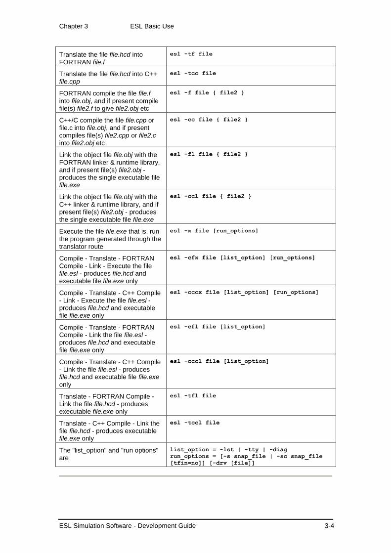
Chapter 3 ESL Basic Use
ESL Simulation Software - Development Guide 3-4
Translate the file file.hcd into FORTRAN file.f
esl -tf file
Translate the file file.hcd into C++ file.cpp
esl -tcc file
FORTRAN compile the file file.f into file.obj, and if present compile file(s) file2.f to give file2.obj etc
esl -f file { file2 }
C++/C compile the file file.cpp or file.c into file.obj, and if present compiles file(s) file2.cpp or file2.c into file2.obj etc
esl -cc file { file2 }
Link the object file file.obj with the FORTRAN linker & runtime library, and if present file(s) file2.obj - produces the single executable file file.exe
esl -fl file { file2 }
Link the object file file.obj with the C++ linker & runtime library, and if present file(s) file2.obj - produces the single executable file file.exe
esl -ccl file { file2 }
Execute the file file.exe that is, run the program generated through the translator route
esl -x file [run_options]
Compile - Translate - FORTRAN Compile - Link - Execute the file file.esl - produces file.hcd and executable file file.exe only
esl -cfx file [list_option] [run_options]
Compile - Translate - C++ Compile - Link - Execute the file file.esl - produces file.hcd and executable file file.exe only
esl -cccx file [list_option] [run_options]
Compile - Translate - FORTRAN Compile - Link the file file.esl - produces file.hcd and executable file file.exe only
esl -cfl file [list_option]
Compile - Translate - C++ Compile - Link the file file.esl - produces file.hcd and executable file file.exe only
esl -cccl file [list_option]
Translate - FORTRAN Compile - Link the file file.hcd - produces executable file.exe only
esl -tfl file
Translate - C++ Compile - Link the file file.hcd - produces executable file.exe only
esl -tccl file
The "list_option" and "run options" are
list_option = -lst | -tty | -diag
run_options = [-s snap_file | -sc snap_file
[tfin=no]] [-drv [file]]
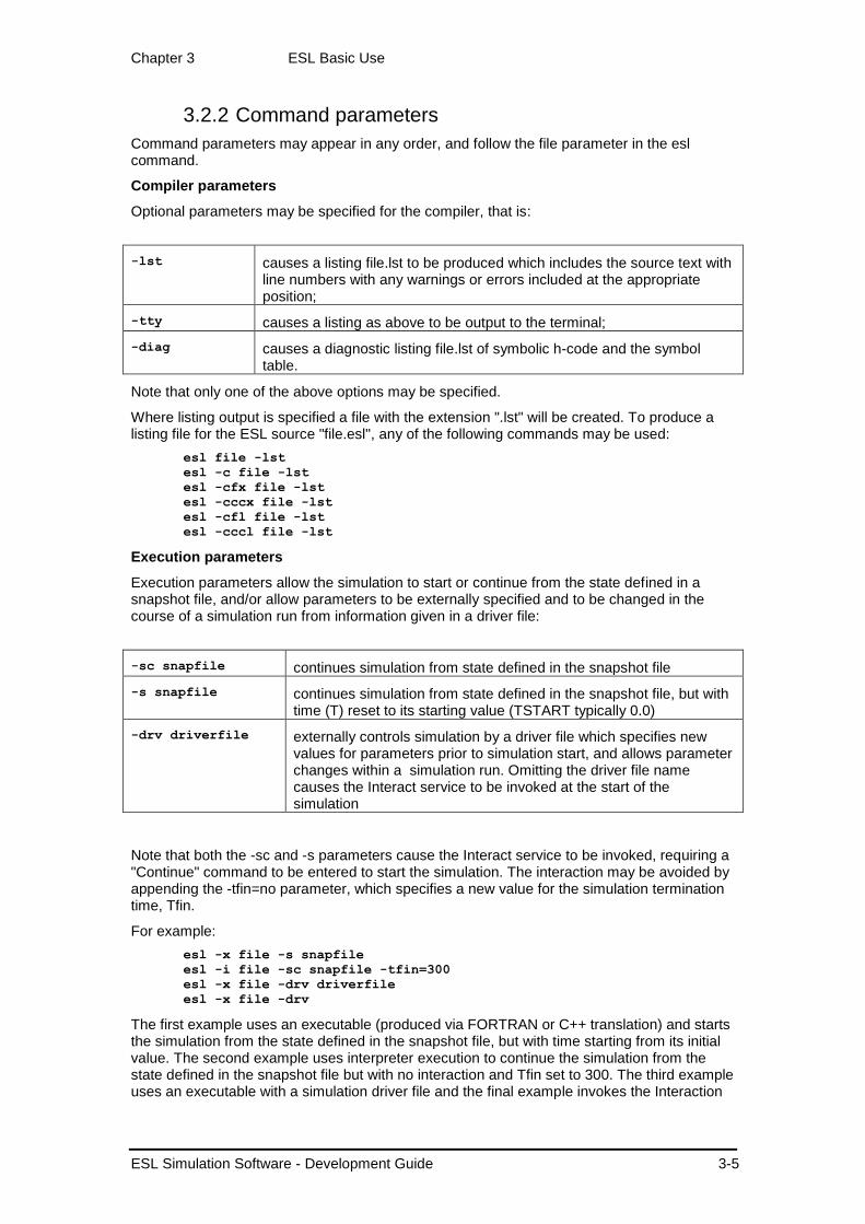
Chapter 3 ESL Basic Use
ESL Simulation Software - Development Guide 3-5
3.2.2 Command parameters
Command parameters may appear in any order, and follow the file parameter in the esl command.
Compiler parameters
Optional parameters may be specified for the compiler, that is:
-lst causes a listing file.lst to be produced which includes the source text with line numbers with any warnings or errors included at the appropriate position;
-tty causes a listing as above to be output to the terminal;
-diag causes a diagnostic listing file.lst of symbolic h-code and the symbol table.
Note that only one of the above options may be specified.
Where listing output is specified a file with the extension ".lst" will be created. To produce a listing file for the ESL source "file.esl", any of the following commands may be used:
esl file -lst
esl -c file -lst
esl -cfx file -lst
esl -cccx file -lst
esl -cfl file -lst
esl -cccl file -lst
Execution parameters
Execution parameters allow the simulation to start or continue from the state defined in a snapshot file, and/or allow parameters to be externally specified and to be changed in the course of a simulation run from information given in a driver file:
-sc snapfile continues simulation from state defined in the snapshot file
-s snapfile continues simulation from state defined in the snapshot file, but with time (T) reset to its starting value (TSTART typically 0.0)
-drv driverfile externally controls simulation by a driver file which specifies new values for parameters prior to simulation start, and allows parameter changes within a simulation run. Omitting the driver file name causes the Interact service to be invoked at the start of the simulation
Note that both the -sc and -s parameters cause the Interact service to be invoked, requiring a "Continue" command to be entered to start the simulation. The interaction may be avoided by appending the -tfin=no parameter, which specifies a new value for the simulation termination time, Tfin.
For example:
esl -x file -s snapfile
esl -i file -sc snapfile -tfin=300
esl -x file -drv driverfile
esl -x file -drv
The first example uses an executable (produced via FORTRAN or C++ translation) and starts the simulation from the state defined in the snapshot file, but with time starting from its initial value. The second example uses interpreter execution to continue the simulation from the state defined in the snapshot file but with no interaction and Tfin set to 300. The third example uses an executable with a simulation driver file and the final example invokes the Interaction

Chapter 3 ESL Basic Use
ESL Simulation Software - Development Guide 3-6
service. Note that the snapshot parameters, driver parameters, and other parameters, may be specified in a combination command, for example:
esl -cccx file -lst -s snapfile -drv driverfile
A full description of the snapshot and the simulation driver file facility is given in ESL Run Control.
3.2.3 Files produced by ESL
Filename extensions are used to identify different file types used by ESL. In the following "filename" is interpreted as the base filename (no extension) of an ESL source code program, "usename" as a base filename specified by the user during ESL execution. Where two alternatives are given the first illustrates the MS Windows convention:
filename.esl ESL source program files in text format
filename.hcd h-code output of the ESL Compiler, containing the Symbol Table as well as the h-code. It is used by the Interpreter to execute a simulation, and by the Translator to generate equivalent FORTRAN/C++ code
filename.lst listing text files are generated by the compiler and takes one of two forms: source code listing with line numbers and compiler messages included; symbolic h-code listing, and symbol table, used mainly by ISIM International Simulation Limited for diagnostic purposes
filename.f FORTRAN source code text file produced by the ESL Translator when invoked by the esl -tf command
filename.cpp C++ source code text file produced by the ESL Translator when invoked by the esl -tcc command
filename.obj object code file produced by the FORTRAN/C++ compiler when invoked by the esl -f/-cc command
filename.exe executable code file produced by linking object and library files and invoked by esl -fl/-ccl/-cfx/-cccx/-cfl/-cccl/-tfl/-tccl command
usename.dsp ESL prepare files which contain graphical data in a form suitable for display using the ISE display manager program
usename.tab ESL tabulate text files which contain tabular data listings
usename.snp snapshot files which contain data defining the state of a simulation at the point the "snapshot" was taken (see ESL Run Control)
filename.rem text file specifying the networked computers and processes which are used to execute remote segments (see ESL Segments)
usename.drv simulation driver file used to set parameters prior to simulation, and during a run (see ESL Run Control)
3.2.4 File access
In ESL filenames must not include spaces. ESL is sensitive to whether filenames are in upper or lower case characters, and on systems that are sensitive to case ESL uses the following rules to open a user specified filename (for example, filenames in INCLUDE statements):
1. try to open (using lower case default extension if no extension specified);

Chapter 3 ESL Basic Use
ESL Simulation Software - Development Guide 3-7
2. try to open (using lower case default extension if no extension specified), but with tree prefix of library directory;
3. try to open "as is" with no default extension.
If none of the above succeeds, the user specified filename is converted to lower case and the complete sequence attempted again.
For case sensitive systems the ESL INCLUDE statement does not make a distinction between upper and lower case. An "INCLUDE LIMINT" will open "LIMINT" if it exists, otherwise it will try to open "limint". On the other hand, the statement "INCLUDE limint" will only attempt to open the lower case filename.
Note that users are strongly advised to use only lower-case file names for all ESL files with case-sensitive operating systems.
On case sensitive systems, best practice is:
Use lower case filenames if possible.
Avoid filenames whose only difference is case.
3.2.5 Using ESL commands
To explain the operation of the "esl" command let us consider the example (rocket) which simulates the vertical flight of a rocket used to sample atmospheric dust at high altitude. The rocket has a mass of 300 Kg, a fuel capacity of 2 000 Kg, produces a constant thrust of 35 000 N and burns fuel at a rate of 20 Kg/s. The aerodynamic drag force always opposes motion and is proportional to the square of velocity. The basic equation of vertical flight is:
ℎ𝑒𝑖𝑔ℎ𝑡′′ =(𝑡ℎ𝑟𝑢𝑠𝑡 − 𝑑𝑟𝑎𝑔)
𝑚𝑎𝑠𝑠− 𝐺
where G is 9.81 m/s2, and the drag proportionality is 0.5 Ns
2/m
2.
The program simulates several flights of the rocket with initial fuel load varying between 1 400 Kg and 2 000 Kg, in order to determine how initial fuel effects the maximum height achieved.
Note that the "rocket" program example is available in the ESL examples directory, as are all main examples in this manual. Examples should be copied to your own working directory before execution.
The program may be run using the ESL compiler and interpreter or compiler and translator commands.
3.2.6 Compiler and Interpreter
To run the compiler and then the Interpreter enter:
esl rocket
This will result in the compiler response:
**** E S L Compiler v8.2.1.xx
**** Copyright (C) ISIM International Simulation Limited 1992-2014.
The compiler produces file rocket.hcd which is used as input to the Interpreter. The Interpreter outputs the following message:
**** E S L Interpreter Run-time v8.2.1.xx
**** Copyright (C) ISIM International Simulation Limited 1992-2014.

Chapter 3 ESL Basic Use
ESL Simulation Software - Development Guide 3-8
The first example - rocket.esl
study
model rocket( real: max_ht := real: FUELo);
-- Output max height, input initial fuel.
real: height,drag,thrust,velocity,FUEL,Mass;
constant real: G/9.81/,Mrk/300.0/,burn/20.0/;
logical: power, done/false/;
initial --Initial conditions.
height:= 0.0; height':= 0.0; FUEL:= FUELo;
max_ht:= 0.0;
dynamic
--Rocket dynamics.
velocity:= height';
-- Drag is proportional to velocity squared.
drag:= 0.5 * velocity * abs(velocity);
-- Mass of rocket and its current fuel.
Mass:= Mrk + FUEL;
-- Do we still have fuel and hence power?
power:= FUEL > 0.0;
-- Thrust is constant until fuel exhausted.
thrust:= if power then 35000.0 else 0.0;
-- Flight equation.
height'':= (thrust - drag)/Mass - G;
-- Fuel Mass equation, fuel burn constant.
FUEL':= if power then -burn else 0.0;
-- Detect maximum height.
when height' < 0.0 then
done:= true;
max_ht:= height; -- record the max.
end_when;
step
-- Save results for later analysis by DISP.
prepare "rocket",t,height,velocity,thrust,
FUEL,drag,Mass;
terminate done; --when rocket starts decent.
communication
Tabulate t,height,velocity;
end rocket;
-- Experiment
real: FUELo, max_ht;
-- Set integration parameters
algo:= rk5; cint:= 15.0; tfin:= 120.0;
-- Do simulation for varying initial fuel.
for FUELo:= 1400.00 .. 2000.0 step 200.0
loop
-- Call the model to do a simulation run.
rocket(max_ht := FUELo);
print "With fuel ",FUELo:6.1," Kg",
" height achieved was ",max_ht:-10.1," m.";
end_loop;
end_study
Output from Interpreter execution of "rocket.esl"
**** E S L Interpreter Run-time v8.2.1.xx
**** Copyright (C) ISIM International Simulation Limited 1992-2014.
T HEIGHT VELOCITY
0.00000E+00 0.00000E+00 0.00000E+00
15.000 1200.2 150.10
30.000 4001.9 210.28
45.000 7317.0 229.59
60.000 10867.0 243.50
75.000 13957.0 56.701
With fuel 1400.0 Kg height achieved was 14087.5 m.

Chapter 3 ESL Basic Use
ESL Simulation Software - Development Guide 3-9
T HEIGHT VELOCITY
0.00000E+00 0.00000E+00 0.00000E+00
15.000 990.85 127.74
30.000 3497.8 195.04
45.000 6629.9 219.33
60.000 10037.0 234.43
75.000 13656.0 247.86
With fuel 1600.0 Kg height achieved was 15647.2 m.
T HEIGHT VELOCITY
0.00000E+00 0.00000E+00 0.00000E+00
15.000 810.35 107.01
30.000 3010.7 177.52
45.000 5931.2 207.80
60.000 9182.3 224.81
75.000 12663.0 239.03
90.000 16348.0 252.20
With fuel 1800.0 Kg height achieved was 17088.8 m.
T HEIGHT VELOCITY
0.00000E+00 0.00000E+00 0.00000E+00
15.000 654.44 88.156
30.000 2546.5 158.12
45.000 5224.3 194.53
60.000 8301.9 214.44
75.000 11636.0 229.72
90.000 15186.0 243.51
105.00 18276.0 56.713
With fuel 2000.0 Kg height achieved was 18407.0 m.
This program output results from the program's TABULATE statement.
The individual operations Compile and Interpret, may be invoked as separate commands. Invoke the Compiler by:
esl -c rocket
and the Interpreter by:
esl -i rocket
3.2.7 Compiler and Translator
The Translator method of executing an ESL program converts a .hcd file into a FORTRAN or C++ source code file with extension .f or .cpp. The following shows the separate sequence of ESL commands to execute a C++ Translated simulation:
Compile the ESL program (not needed if the file rocket.hcd already exists from previous compilation)
esl -c rocket
Translate the h-code in rocket.hcd to C++ in file rocket.cpp:
esl -tcc rocket
The C++ source file has to be compiled. For this use:
esl -cc rocket
which produces file rocket.obj or rocket.o, and then the linking process:
esl -ccl rocket
links the object code with the necessary library routines to produce an executable C++ file, rocket.exe or rocket.

Chapter 3 ESL Basic Use
ESL Simulation Software - Development Guide 3-10
Finally, to run the program:
esl -x rocket
Depending on the type and complexity of operations in the ESL program, considerable reductions in execution time may be obtained by using the translator.
The above operations may be combined in logical sequence:
To compile, translate, C++ compile and link:
esl -cccl rocket
To translate, C++ compile and link:
esl -tccl rocket
To compile, translate, C++ compile, link and execute:
esl -cccx rocket
The equivalent FORTRAN command, to compile, translate, FORTRAN compile, link and execute is:
esl -cfx rocket
3.2.8 User interaction
When running an ESL program independently of ISE, an on-line run-time support facility is provided which allows the user to halt the run, examine and if necessary modify variables or abort the run. This is known as the "INTERACT" facility and is invoked by the break key combination - Ctrl + Break on a PC (usually Ctrl + C on other computers). INTERACT statements may be placed in the program to activate this service. This facility is simple to use, typing "HELP" or gives a menu of options (see ESL Run Control for further information).
3.2.9 Post Run graphical analysis
The simulation execution also created a prepare file rocket.dsp, defined by the "prepare" statement in rocket.esl, which contains the values of t (time), height and velocity etc, throughout the simulation.
This data may be viewed graphically by the Post Run Plot option of the ISE Display Manager as part of a simulation "post-mortem" analysis. The figure shows an ISE Post Run Plot graph of results obtained from running the rocket program.
The ISE Post Run Plot option provides "post-mortem" graphical analysis of ESL simulation results. It processes .dsp files produced by the ESL prepare statement (or prepare files specified directly from ISE). Conversion facilities are also provided, through the ISE File menu, to convert tabulate format text files into the prepare format (see ISE File menu - Display Conversion). The prepare file can also be plotted or converted to another format using the convertDisplayFile program.

Chapter 3 ESL Basic Use
ESL Simulation Software - Development Guide 3-11
Post-Run plot of "rocket" results
3.3 An ESL Program - Line-by-Line
The program
Lexical components
Comments
Include files
Program structure and modules
PACKAGE definition
Reserved PACKAGE
Run specification
Integration selection
Model definition
Results from the ESL example
3.3.1 The program
This section provides an introduction to the ESL language by introducing a second example, Bench3, which is provided in the ESL example directory. The program illustrates many of the basic ESL features and the remainder of this section examines, line by the line, the components of the program. The listing in Bench3 contains line numbers for identification only - these are not part of the program.
The example is somewhat artificial in order to demonstrate as many features of the ESL language as possible. It comprises three different solutions of the Van der Pol equation, (represented by the variables X, Y and Z). that is:
𝑥′′ = 𝑘(1 − 𝑥2)𝑥′ − 𝑥
The Van der Pol equation can be considered to simulate the output of an electronic oscillator. The variable absX represents the absolute value of X, and models the output of a perfect full-wave bridge rectifier which is subject to an input waveform X (output of the Van der Pol oscillator). The variables XMAX and XMIN are designed to save the maximum and minimum values of the waveform described by X which occur during the course of a simulation run.

Chapter 3 ESL Basic Use
ESL Simulation Software - Development Guide 3-12
The first task of the ESL Compiler is to analyze the syntax of the source program and this is done at several levels. A given statement is examined at the lexical level to determine the lexical components; then the statement structure is analyzed; finally a check is made to determine whether a statement may legally appear at that point in the overall structure of the program. Here, we shall continue this "bottom up" approach to introduce the basic ESL features - we shall study the lexical components, and then the statement structure. ESL is explained using a "top down" approach in ESL Operation and Program Structure.
Sample Program - bench3.esl
0001 --Benchmark 3
0002 STUDY
0003 PACKAGE GLOBAL; REAL:ARR(5,2); INTEGER:RUN/0/; END;
0005 PROCEDURE FUN(REAL:CONST,VAR)RETURN REAL;
0006 REAL:SQUARE; SQUARE:=1-VAR**2; RETURN CONST*SQUARE;
0007 END FUN;
0008 --
0009 SUBMODEL INTGL(Real: out:= CONSTANT Real: IC; Real: in);
0010 INITIAL out:=IC; DYNAMIC out':=in;
0011 END INTGL;
0012 --
0013 INCLUDE "integ";
0014 --
0015 MODEL VanderPol(Real: X,Y:=Real: K);
0016 USE GLOBAL;
0017 CONSTANT REAL: XD0/0.0/;
0018 REAL: Z,XMAX,XMIN/0.0/,absX;
0019 INITIAL
0020 X:=0.1; X':=XD0; XMAX:=0;
0021 DYNAMIC
0022 X'':= FUN(K,X)*X'-X;
0023 Y := INTEG(X,X'); --Library submodel (same as INTGL)
0024 Z := INTGL(0.1,X');
0025 absX := if X >= 0.0 then X else -X;
0026 when X' < 0.0 then
0027 if X > XMAX then XMAX:= X; end_if;
0028 when X' >= 0.0 then
0029 if X < XMIN then XMIN:= X; end_if;
0030 print "Minimum ",X :-13.5," detected at T= ",T :-13.5;
0031 end_when;
0032 STEP
0033 PREPARE "bench3",T,X,X',X'',absX,Y,Z;
0034 COMMUNICATION
0035 PLOT "Phase plane plot",X,X',-2.0,2.0,-2.0,2.0;
0036 TERMINAL
0037 RUN:=RUN+1; ARR(RUN,1):=K; ARR(RUN,2):=XMAX;
0038 PRINT "Run no, Xmax, Xmin: ",RUN,XMAX,XMIN;
0039 END VanderPol;
0040 --
0041 --EXPERIMENT
0042 USE GLOBAL;
0043 REAL: X,Y,K/1.0/; INTEGER:I;
0044 READ ALGO,CINT,NSTEP;
0045 TFIN:=10;
0046 WHILE RUN < 5
0047 LOOP
0048 VANDERPOL (X,Y:=K); K:= K+0.5;
0049 INTERACT;
0050 END_LOOP;
0051 PRINT " RUN NO. K XMAX";
0052 FOR I:=1..RUN
0053 LOOP PRINT I, ARR(I,1),ARR(I,2); END_LOOP;
0054 END_STUDY

Chapter 3 ESL Basic Use
ESL Simulation Software - Development Guide 3-13
3.3.2 Lexical components
A principal characteristic of an ESL program is a lexical style that is similar to that of an Ada or Pascal program. Semicolons are used to separate statements, and all identifiers are specified, or declared, before they are used. A number of general points about ESL's basic lexical components need to be made before proceeding to a discussion of the program and statement structure.
Identifiers
Identifiers may consist of any number of letters and digits but only the first 28 characters are significant. The first character must be a letter. Identifiers differing only in the use of corresponding upper and lower-case letters are considered the same. The underscore symbol "_" may be used within an identifier to improve the appearance.
Primes (') appended to an identifier indicate first or higher-order derivatives of the variable (for example, x', pos"). The identifier plus appended primes must not be longer than 28 characters. Identifier examples:
VELOCITY X1 x2 Torque x' POS" Velocity_sat_1
Numbers
There are two classes of number - integers (whole numbers) and reals (floating point numbers). The range of an integer is -2
31 to (2
31-1), and the magnitude of a real is in the
approximate range 10-38
to 10+38
for single precision and 10-308
to 10+308
for double precision (see below). A real number must contain a decimal point, which may never be the first or last character of a number. It must always be preceded by a digit and followed by either a digit or an exponent "E" or "D" part. Examples:
12 12.0 12.E0 12E0 1.2E+01 0.12D2
The D and E exponent characters are treated identically - all real numbers are held to single precision by the ESL interpreter, FORTRAN translated and single precision C++ programs; all real numbers are held to double precision by default for C++ translated programs.
Both reals and integers may be signed, but must not contain embedded spaces.
Character strings
A literal character string is a sequence of characters enclosed by string bracket characters ( " or % ).
"This is a string"
%SO IS THIS%
To use the string bracket character itself within a string, the alternative string bracket characters should enclose the string, or it should be written twice. Thus the string -A HIGH %- could be written as:
"-A HIGH %-"
or
%-A HIGH %%-%.
Statements and expressions
ESL contains a variety of statement types, which are described in detail in ESL Operation and Program Structure. Note that a line of code may contain multiple statements and that statements are terminated by a semicolon ";". A statement may also be continued over several lines.

Chapter 3 ESL Basic Use
ESL Simulation Software - Development Guide 3-14
The ESL expression is consistent with that defined in other languages such as FORTRAN, but the relational operators are represented as:
= equal to
/= not equal to
> greater than
< less than
<= less than or equal to
>= greater than or equal to
3.3.3 Comments
Comments start with a double hyphen "--" and are terminated by the end-of-line. Lines 1, 8, 12, 14, 40, 41 in Bench3 are all comment lines, and line 23 contains a comment.
Library comments
The LIBRARY comment is a special comment used only by ISE when processing ESL text submodels, or function procedures. It is used to specify any standard library submodel, other submodel, procedure, or package, which is used by that module. It causes ISE to generate INCLUDE statements to incorporate the required modules.
The general form of the Library comment is:
-- LIBRARY file1, file2, file3
where file1, file2, file3 etc are the sources of the module referred to.
Its use is illustrated in the following example that uses the standard library submodel stepp:
SUBMODEL example( ... := ... );
-- LIBRARY stepp
LOGICAL: log1;
INITIAL
DYNAMIC
log1 := stepp(0.1);
END example;
Note that any LIBRARY comments must be placed immediately after the submodel declaration statement.
3.3.4 Include files
ESL source code may be "included" from a file and inserted into the program by the use of an INCLUDE statement. Include statements may appear at any point in a program as the only statement on a line, with no following comment. They are dealt with at the lexical level. Line 13 of Bench3 contains an include statement which causes the submodel library module INTEG to be included from the ESL library directory, for example:
INCLUDE "filename1";
INCLUDE "filename2" -l;
The literal character strings (filename1/2) specify the name of the file which is to be included at that point in the program. ESL will conduct a search for INCLUDE files starting in the local directory and then the ESL library directory as follows:
If an explicit extension is given, .esl or an alternative, a search will be made first in the current directory and then in the ESL library directory.
If no extension is given, the following sequence is used:
Current directory, .esl extension.
Library directory, .esl extension.
Current directory, no extension.

Chapter 3 ESL Basic Use
ESL Simulation Software - Development Guide 3-15
The "-l " option causes the include file statements to be listed if a listing is requested when compilation is started.
Include files may be nested (that is, the included files may in turn contain INCLUDE statements).
3.3.5 Program structure and modules
The structure of an ESL program is illustrated by "bench3". The keywords STUDY on line 2 and END_STUDY on line 54, bracket the program modules. We shall see in ESL Operation and Program Structure that other possibilities exist, but for the moment we shall assume that all ESL programs begin and end with these keywords. The "bench3" example shows five of the principal constructs of ESL:
The MODEL, (line 15 to 39).
The SUBMODEL, (line 9 to 11).
The EXPERIMENT, (line 41 to 53).
The PROCEDURE, (line 5 to 7).
The PACKAGE, (line 3).
Each of these modules has a particular purpose which will be described in turn below. The model and submodel is where the dynamic aspects of ESL simulation are defined, and the other modules support this. The experiment is the default region - if no other modules are declared between STUDY and END_STUDY, then all statements will be in the experiment module, or region. Note that experiment is not a keyword, and the comment on line 41 is for clarity only. When ESL is run, the experiment region is executed first and this almost always involves calling the model, the module immediately above. One rule in ESL is that all modules must be declared before they are used, so it can be seen that the most widely used structures, such as PACKAGE which involves common data, are declared first, whereas the model is only used by the experiment and can therefore be the last non-experiment module to be presented.
The experiment controls the running of the model, or models, in the study. Setting parameters which control the simulation, such as integration algorithm, step-length, communication interval, final-time and error tolerances, is often done here. Alternatively the model INITIAL region may be used to set these parameters. The complete language provides a variety of procedural code statements, including loop and conditional statements to allow easy programming of sequences of runs.
In common with all ESL program modules, data variables must be declared before they are used. The USE GLOBAL statement in line 42, that is:
0042 USE GLOBAL;
specifies that the data variables defined in the PACKAGE GLOBAL are available to the experiment. Local variables X, Y, and K are declared as type REAL, and I as type INTEGER, in line 43, that is:
0043 REAL: X,Y,K/1.0/; INTEGER:I;
The real variable K is declared to have an initial value of 1.0 which is set once prior to program execution. Variables may be defined as type REAL, INTEGER, LOGICAL, CHARACTER or FILE (see ESL Operation and Program Structure). Declared variables must be different from the ESL reserved words.
The experiment and the modelling subprograms (model, submodel, or segment) are all assumed to have an implicit USE RESERVED statement which gives the program module access to ESL's reserved variables. This is the only example in ESL where variables do not have to be explicitly declared. The reserved variables include simulation time (T), start time (TSTART), finish time (TFIN), communication interval (CINT), integration algorithm (ALGO) and minimum number of integration steps in a communication interval (NSTEP).
In the example, the READ statement in line 44, that is:

Chapter 3 ESL Basic Use
ESL Simulation Software - Development Guide 3-16
0044 READ ALGO,CINT,NSTEP;
causes the user to be prompted to input values for ALGO, CINT and NSTEP. Suitable values are ALGO=1 (to select the default variable-step fifth-order integration algorithm), CINT=0.1 (communication points or primary output every 0.1 second), and NSTEP=1 (maximum integration step-length of CINT). In response to the prompt for ALGO the user may enter an integer value followed by return, and then the user is prompted for the remaining input (CINT and NSTEP). Alternatively the user may enter all three values separated by spaces, or commas, in response to the "ALGO," prompt, for example:
ALGO,CINT,NSTEP:1,0.1,1
The assignment statement in line 45 uses the ":=" assignment operator to indicate that the reserved variable TFIN is set equal to 10, that is:
0045 TFIN:=10;
A WHILE-loop occupies lines 46 to 50:
0046 WHILE RUN < 5
0047 LOOP
0048 VANDERPOL (X,Y:=K); K:= K+0.5;
0049 INTERACT;
0050 END_LOOP;
and this causes the body of the loop to be repeated while the variable RUN, declared in PACKAGE GLOBAL, is less than 5. As RUN is initialised with zero, and incremented at the end of each simulation run (model line 37), the body of the loop will be executed 5 times.
The body of the loop includes an invocation, or call, to the model VANDERPOL, in line 48, which causes a single simulation run of the model. The arguments X and Y are model outputs, which must be separated from the model input argument K by the assignment operator ":=". Note that K is increased after each simulation run.
The model invocation is followed by an INTERACT statement which invokes the on-line interact support service. This provides an aid to program development and testing, and affords a simple mechanism for the user to control simulation experiments. A number of commands are available to: examine or set data variables; determine the state of the program; or to control subsequent execution, for example, continue the simulation, restart the simulation from the beginning or simply "quit". It is designed to provide the user with all the information necessary to perform the above tasks. By typing HELP and then pressing Return or Enter key, a list of commands and explanations are given. A full description of is given in ESL Run Control.
Following the simulation loop, lines 51 to 53 contain a PRINT statement to output a title, and then a simple FOR-loop to output K and corresponding maximum value of X for each simulation run, that is:
0051 PRINT " RUN NO. K XMAX";
0052 FOR I:=1..RUN
0053 LOOP PRINT I, ARR(I,1),ARR(I,2); END_LOOP;
The appropriate values for output have been saved in the array ARR during the course of the simulation runs. The END_STUDY statement in line 54 causes the program to stop.
3.3.6 PACKAGE definition
Line 3 defines the PACKAGE with the name GLOBAL, and specifies package variables ARR, a real array, and RUN, an integer variable, that is:
0003 PACKAGE GLOBAL; REAL:ARR(5,2); INTEGER:RUN/0/; END;
This means of specifying variables is similar to FORTRAN common, but in ESL program modules package data is accessed by the USE statement (for example, lines 16 and 42) rather than by the user repeating a declaration. Unlike FORTRAN common a package may be used to give initial values to variables (for example, RUN is initialised with the value zero).
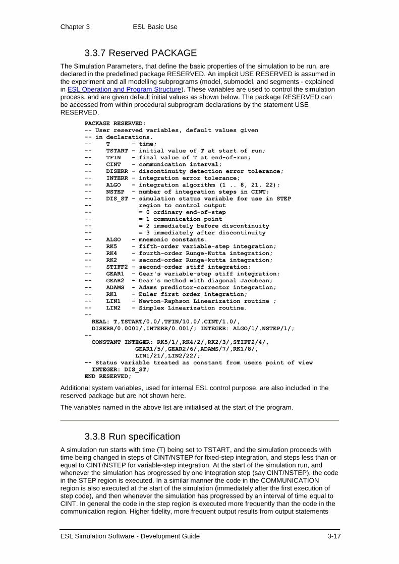
Chapter 3 ESL Basic Use
ESL Simulation Software - Development Guide 3-17
3.3.7 Reserved PACKAGE
The Simulation Parameters, that define the basic properties of the simulation to be run, are declared in the predefined package RESERVED. An implicit USE RESERVED is assumed in the experiment and all modelling subprograms (model, submodel, and segments - explained in ESL Operation and Program Structure). These variables are used to control the simulation process, and are given default initial values as shown below. The package RESERVED can be accessed from within procedural subprogram declarations by the statement USE RESERVED.
PACKAGE RESERVED;
-- User reserved variables, default values given
-- in declarations.
-- T - time;
-- TSTART - initial value of T at start of run;
-- TFIN - final value of T at end-of-run;
-- CINT - communication interval;
-- DISERR - discontinuity detection error tolerance;
-- INTERR - integration error tolerance;
-- ALGO - integration algorithm (1 .. 8, 21, 22);
-- NSTEP - number of integration steps in CINT;
-- DIS_ST - simulation status variable for use in STEP
-- region to control output
-- = 0 ordinary end-of-step
-- = 1 communication point
-- = 2 immediately before discontinuity
-- = 3 immediately after discontinuity
-- ALGO - mnemonic constants.
-- RK5 - fifth-order variable-step integration;
-- RK4 - fourth-order Runge-Kutta integration;
-- RK2 - second-order Runge-kutta integration;
-- STIFF2 - second-order stiff integration;
-- GEAR1 - Gear's variable-step stiff integration;
-- GEAR2 - Gear's method with diagonal Jacobean;
-- ADAMS - Adams predictor-corrector integration;
-- RK1 - Euler first order integration;
-- LIN1 - Newton-Raphson Linearization routine ;
-- LIN2 - Simplex Linearization routine.
--
REAL: T,TSTART/0.0/,TFIN/10.0/,CINT/1.0/,
DISERR/0.0001/,INTERR/0.001/; INTEGER: ALGO/1/,NSTEP/1/;
--
CONSTANT INTEGER: RK5/1/,RK4/2/,RK2/3/,STIFF2/4/,
GEAR1/5/,GEAR2/6/,ADAMS/7/,RK1/8/,
LIN1/21/,LIN2/22/;
-- Status variable treated as constant from users point of view
INTEGER: DIS_ST;
END RESERVED;
Additional system variables, used for internal ESL control purpose, are also included in the reserved package but are not shown here.
The variables named in the above list are initialised at the start of the program.
3.3.8 Run specification
A simulation run starts with time (T) being set to TSTART, and the simulation proceeds with time being changed in steps of CINT/NSTEP for fixed-step integration, and steps less than or equal to CINT/NSTEP for variable-step integration. At the start of the simulation run, and whenever the simulation has progressed by one integration step (say CINT/NSTEP), the code in the STEP region is executed. In a similar manner the code in the COMMUNICATION region is also executed at the start of the simulation (immediately after the first execution of step code), and then whenever the simulation has progressed by an interval of time equal to CINT. In general the code in the step region is executed more frequently than the code in the communication region. Higher fidelity, more frequent output results from output statements

Chapter 3 ESL Basic Use
ESL Simulation Software - Development Guide 3-18
placed in the step region. On the other hand, output from the communication region is always at regular intervals determined by the user setting CINT.
A simulation with the independent variable decreasing (integration with time decreasing as the simulation progresses) occurs when TFIN is less than TSTART, and the communication interval, CINT, is negative.
Run Termination - TERMINATE
A run terminates in the following three circumstances:
(1) After the communication interval (end of communication region) in which time, T, has become equal to, or greater than, TFIN. This check also applies if the simulation is in reverse, and time is decreasing as the simulation proceeds.
(2) Following successful execution of a TERMINATE statement placed in the step or communication region. The simulation run is terminated following the execution of the step or communication region in which the terminate condition is satisfied. For the statement:
TERMINATE T >= 16.33333;
the value of T at termination will be that corresponding to the step or communication point, that is, normally T will be greater than the specified terminate value.
(3) Following successful execution of TERMINATE statement placed in the body of "when" statement, for example:
when T >= 16.33333 then terminate TRUE; end_when;
will cause terminate to occur more precisely. A step region is executed at T "very close" to the expected value prior to run termination.
Understanding CINT, ALGO, TSTART and TFIN
CINT may be changed during a simulation run, and the next communication interval will use the new value of CINT. Note the current communication interval is first completed with the previous CINT, and the next communication interval uses the new value. Changes to NSTEP also take effect in the same manner.
The value of TSTART which is current after the final statement of a model (or segment) INITIAL region, is taken as the start time for the simulation run. Any subsequent changes, for example, in a submodel INITIAL region, or any other code section, do not influence the start time for the current run. Similarly the value of ALGO (integration method) which is current when the first integration step is started is used for the current run. Changes made to ALGO during a run do not influence the current run.
Note that in INITIAL regions TSTART should be used instead of T to indicate a value for time. At the start of the model/segment INITIAL region T is set to the existing value of TSTART, and at the end of INITIAL region T is again set to TSTART (this allows users to set TSTART in the INITIAL region). Users may freely change TFIN during the course of a run.
A simulation may proceed in a reverse sense, that is, with time decreasing. To program a reverse time run, set CINT negative and ensure TFIN is less than TSTART. Programs that depend on time related events (for example, the ESL modulator library submodel - modult), cannot be simulated with time decreasing.
During the implicit INTERACT service mode, at the point where INTERACT is automatically invoked at end-of-run (at TFIN), the run may be extended either with time increasing or decreasing. In this case simply ensure CINT is set to indicate the direction of simulation, and issue "Continue xxx", where xxx is the new TFIN required. Note a simple "Continue" at this point will cause the simulation run to be terminated, even though TFIN may just have been interactively changed.
3.3.9 Integration selection
The integration algorithm to be used in a simulation run is determined by setting the reserved variable ALGO. This variable may be set to an integer value, or a predefined symbolic name.

Chapter 3 ESL Basic Use
ESL Simulation Software - Development Guide 3-19
The following table gives the different integer values allowed for ALGO and the corresponding symbolic name:
1 or RK5 - fifth-order variable-step integration;
2 or RK4 - fourth-order Runge-Kutta integration;
3 or RK2 - second-order Runge-Kutta integration;
4 or STIFF2 - second-order stiff integration;
5 or GEAR1 - Gear's variable-step stiff integration;
6 or GEAR2 - Gear's method with diagonal Jacobean;
7 or ADAMS - Adams predictor-corrector integration;
8 or RK1 - Euler first-order integration.
Note that the following statements are equivalent:
ALGO:= 5;
ALGO:= GEAR1;
The reader is referred to a detailed description of integration given in Modelling Code. Two other mnemonics are also permitted for ALGO, these are LIN1 and LIN2 which specify the method for determining steady-state conditions when the model ANALYSIS region is used (see Steady-State Analysis).
3.3.10 Model definition
The model provides the user with the means to describe the physical system, and may contain information relating to how a single simulation run is to be performed. It is the model through its dynamic region code, and invocations of submodels and segments, that defines the complete physical system to be simulated.
A model definition starts with a model declaration statement which specifies the name, output and input arguments of the model. Declarations follow and finally the model definition ends with the model body, which must contain at least a DYNAMIC region, and may also include INITIAL, TERMINAL and ANALYSIS regions. The DYNAMIC region may call previously defined submodels, and may optionally have associated COMMUNICATION and STEP regions.
Model statement
The model declaration in line 15, that is:
0015 MODEL VanderPol(Real: X,Y:=Real: K);
specifies the name of the model is VANDERPOL, and it has two REAL output arguments, X and Y and one REAL input argument, K. This means that the experiment (see line 48), sets the value of K to be used by the MODEL, which returns values of X and Y to the experiment.
Declarations
Lines 16 to 18 declare variables local to the MODEL, and in some cases initialise them, that is:
0016 USE GLOBAL;
0017 CONSTANT REAL: XD0/0.0/;
0018 REAL: Z,XMAX,XMIN/0.0/,absX;
All variables and constants used in the MODEL must be declared. Note that the input and output variables (arguments) are declared in the MODEL declaration; the reserved variable T is declared in the predefined PACKAGE RESERVED and made accessible by an implicit USE RESERVED statement; and the data variables declared in the PACKAGE GLOBAL are made accessible by the explicit USE GLOBAL statement in line 16.
Consider the statement in line 17. This simply declares a constant REAL identifier, XD0, and sets its value to real zero. Constants must be given a value when declared, and may be defined as type REAL, INTEGER, LOGICAL, or CHARACTER.
The statement in line 18 declares four real variables (Z, XMAX, XMIN, and absX), but only XMIN is specified as having an initial value, (real zero). It is important to appreciate that this

Chapter 3 ESL Basic Use
ESL Simulation Software - Development Guide 3-20
initialisation occurs "every time" the model is invoked, that is, at the start of each simulation run. Whereas initialisation in procedural modules, including the experiment, occurs at the start of program execution, and is a once only operation.
Model body
The output from the model is the value of X and Y at the end of the simulation, and they are specified as output arguments in the model specification statement in line 15. The outputs are two of the solutions of the equation, and they should be equal. The equation to be solved has a parameter K, which is set in the experiment, hence its appearance as an input argument in the model definition statement.
The following examines the DYNAMIC region, and its associated STEP and COMMUNICATION regions, before considering the optional INITIAL and TERMINAL regions.
Dynamic region
The DYNAMIC region specifies the dynamic system to be simulated, and is unlike any other section of an ESL program. It has the task of specifying the parallel processes which occur in a real-life system. In a real system an amplifier which drives the field current of an electric motor is "amplifying" at the same time as the motor is "revolving". The two dynamic operations are happening at the same time, or in parallel. Normal scientific program, or procedural, code which is obeyed strictly in sequence, one statement after another, is not appropriate to describe these parallel operations.
ESL uses special model (non-procedural) code to represent a dynamic system. Each statement represents a separate physical parallel element of the real system, for example:
P:= A + 0.1 * B;
represents an element with output P, which is computed from the inputs A, 0.1 and B according to the expression, and statement:
A,B:= subsys(P);
represents an element with outputs A and B which are computed from input P. In this case subsys is a submodel which may represent a complex sub-system. Note that the output, P, of the first statement is used as an input in the second, and the outputs of the second statement, A and B, are used as inputs in the first statement. These two statements represent physical elements and their interconnection is shown in the figure.
Parallel processing requirement
The order in which the two boxes (statements) are considered is not dictated from the connection diagram. When expressed in ESL the statements may be presented in any order. This is true in general: statements in the model description part of the DYNAMIC region may be presented in any order.

Chapter 3 ESL Basic Use
ESL Simulation Software - Development Guide 3-21
Note that ESL automatically sorts the statements into an appropriate computational order. In order to do this it takes note of the class of the variables - in this illustration the submodel "subsys" is assumed to give variables A and B the property of "inherited memory" variables. Statement sorting, and the terms "class" and "inherited memory" are explained in ESL Operation and Program Structure.
Having established the difference between procedural and model code statements let us examine the example in more detail, statement by statement.
The first presentation of the Van der Pol equation is a single second-order differential equation in line 22 which generates the value X. The differential equation must be arranged in the form of an assignment of a value to the highest derivative (X"), and expressing the Van der Pol equation in this way gives:
X'' := K * (1 - X ** 2) * X' - X;
In line 22 part of the computation of the expression is undertaken in the procedure FUN, described below, and the statement reduces to:
0022 X'' := FUN(K,X)*X'-X;
This presentation specifies to ESL that X is determined by subjecting the variable X'' to an integration process to obtain X', and then subjecting X' to a second integration process to obtain X. Whenever integration is performed it is necessary to specify the initial value, or condition, of the "state" variable which will contain the result of the integration. As both X and X' are state variables obtained as a result of an integration, both variables must be given initial values. The assignment statements in the INITIAL region, line 20, initialise X to the real value 0.1 and X' to zero. The INITIAL region is executed prior to the start of each simulation run.
State variables, which contain the result of an integration, are also known as memory variables. This is because their current value depends on the past, or history, and not on the current values of simulation variables. That is, these variables have "memory" of the past. Note that the rate-of-change of a state variable (for example, X'') depends on an algebraic computation involving current values of simulation variables, and such variables are classified as "algebraic" variables.
The second solution of the equation is obtained from the statement in line 23, that is:
0023 Y := INTEG(X,X'); --Library submodel (same as INTGL)
The library submodel INTEG has been included in the study by the use of the INCLUDE "integ" statement in line 13. It is used to integrate X', starting with an initial condition of X. The first input argument of the submodel call, X, is used by the submodel as an initial condition for the integration. Although X changes during the course of the simulation run, the submodel only uses the argument X during its initial region and prior to starting the simulation. It uses 0.1, the initial value of X - therefore, as the initial condition which is the initial value for the output Y. The second input argument, X', which is the variable to be integrated, is generated during the solution of X in line 22. The submodel's output is Y whose value is the result of the integration, and Y is classed as an "inherited state" variable because it has inherited the state property (computed as a result of an integration) from the submodel INTEG. Submodels that have outputs which are the result of integration, have the responsibility of setting the initial condition of those outputs.
The ESL compiler checks that actual arguments, that is the output argument Y and the input arguments X and X', are consistent with regard to type and dimension with the formal arguments in the submodel declaration. Furthermore it checks that the actual arguments are consistently used, for example, that Y has not been set elsewhere in the model.
For submodels with more than one output argument the following style of presentation is used:
P,Q,R:= SUB3OUT(A,B);
In this case P, Q and R are all output arguments of the submodel SUB3OUT.
Note that a submodel invocation (call) statement always appears in the forms shown, and should never be part of an expression. The following statement is illegal:

Chapter 3 ESL Basic Use
ESL Simulation Software - Development Guide 3-22
Y:= A * INTEG(X,X'); -- ILLEGAL
The final presentation of the equation, in line 24, is almost identical to the second presentation, that is:
0024 Z := INTGL(0.1,X');
In this case the submodel INTGL has been explicitly presented in lines 9 to 11, and is functionally identical to the library submodel INTEG. The only other difference is that the initial condition of 0.1 is explicitly presented as the first input argument. Note that the formal input argument IC, line 10, is declared as CONSTANT REAL, which means that its value is constant throughout a simulation run. Even if the actual argument changes it has no further influence on the submodel operation, because the constant declaration ensures only the initial value of the argument is used. In this case IC is only used in the INITIAL region, and clearly should be regarded as constant for the duration of the simulation run.
The absolute value of X (absX) is computed in line 25 where an IF-clause is used, that is:
0025 absX := if X >= 0.0 then X else -X;
The IF-clause is a means of specifying a switching operation, or a simple discontinuity. In this case the IF-clause switches (or sets) absX to be equal to the value of X or -X depending whether the logical expression is true or false (X >= 0.0). While X is positive absX takes the value of X, otherwise it takes the value of minus X.
The instant of switching, when X >= 0.0 changes its logical value, is detected after the actual point of transition, but within a specified error bound. This means that at the point of detection the discontinuity has just occurred and the value of X is nominally zero, that is, it is less than the specified error bound. The user may change the error bounds by setting the reserved variable DISERR (see the discussion of error bounds in Modelling Code).
The variable absX is classified as an algebraic variable because its value depends on an algebraic computation involving the current values of other model variables.
Two WHEN blocks follow in lines 26 to 31, that is:
0026 when X' < 0.0 then
0027 if X > XMAX then XMAX:= X; end_if;
0028 when X' >= 0.0 then
0029 if X < XMIN then XMIN:= X; end_if;
0030 print "Minimum ",X :-13.5," detected at T= ",T :-13.5;
0031 end_when;
The first block, lines 26 to 27, could have been terminated by an END_WHEN after line 27, but as it is followed by a second WHEN block, lines 28 to 31, the END_WHEN may be optionally omitted. Although the two blocks are concatenated they operate as two separate WHEN blocks.
The WHEN block is an alternative method of specifying discontinuities, in which the instant of the transition of the logical expression, rather than the logical state of the expression, is of interest. The body of the first WHEN block, line 27, is executed only at the instant when the logical expression X' < 0.0 becomes true. When X' < 0.0 becomes true, X is a maximum - the rate-of-change of X has changed from a positive value, become zero, and is now negative, so reducing X from its maximum value.
The body of the WHEN block comprises procedural statements, and in the body of the first WHEN block, line 27, the value of X is tested to determine if the maxima just detected is the largest that has occurred at this point in the simulation run.
The second WHEN block performs a similar function to determine the minimum value of X, but in this case it also prints the minimum value detected and the time (T) at which it was detected. The two format control elements (:-13.5) in the PRINT statement indicates that the variables X and T are to be output with a maximum field width of 13 characters, 5 significant figures, and the minus sign indicates that spaces are to be suppressed.
The detection mechanisms used for discontinuities occurring in a WHEN statement are the same as those used for IF - clause discontinuities. The point at which a WHEN body is executed is always immediately after the actual instant the WHEN logical expression became

Chapter 3 ESL Basic Use
ESL Simulation Software - Development Guide 3-23
true. Note that WHEN statements do not become active until the simulation is underway, that is, they are not triggered at the starting time of the simulation run.
The WHEN statements have been used to define the simulation parameters XMIN and XMAX. Variables are classed as simulation parameters when they are initialised prior to entering the dynamic region, and changed, or updated, within the body of a WHEN statement. Parameters are memory variables, like state variables, as they remain constant during an integration step with a value that depends on the past, or history, rather than on other current values. At a discontinuity ESL performs additional computations (extra passes of the dynamic region) to update the values of simulation parameters before proceeding with the simulation.
Step region
The step region, line 32 to 33, that is:
0032 STEP
0033 PREPARE "BENCH3",T,X,X',X'',absX,Y,Z;
is executed at the start of a simulation run, and after each integration step, that is at least NSTEP times for each communication interval. This region is expressed using procedural code statements, and gives the user the opportunity to output results at the maximum frequency as the simulation proceeds. This region is executed immediately before and after a discontinuity so enabling the exact result of switching operations to be observed. Note the value of the reserved variable DIS_ST indicates why the STEP region has been invoked, that is: ordinary step (0); communication point (1); before a discontinuity (2); or immediately after a discontinuity (3). This enables users to select the output that is required.
The PREPARE statement is used to save all the STEP results contained in the listed variables. The file bench3.dsp is created which contains the results of all (5) runs. Note that ESL appends the extension .dsp if none is specified. The Post Run Plot option of the ISE Display Manager may be used to perform post-mortem graphical analysis of the results prepared during a simulation session.
Communication region
The COMMUNICATION region is also expressed in terms of procedural code statements, and is the place to specify the input and output to be made at each communication point. That is at the start of a simulation run, and then at regular intervals of simulated time equal to CINT.
In this case a PLOT statement specifies that a graph is plotted as the simulation proceeds:
0034 COMMUNICATION
0035 PLOT "Phase plane plot",X,X',-2.0,2.0,-2.0,2.0;
The graph will have the title "Phase plane plot", and plot X on the horizontal axis, and X' on the vertical axis. The four numbers specify the lower and upper axis limits for the horizontal and vertical axis respectively.
Additional variables may be simultaneously plotted on the same axes during a simulation run, for example:
PLOT T,X [X', absX] 0,TFIN,-4.0,4.0;
In this case X, X' and absX are all plotted against T, and the optional title specification has been omitted.
A statement that is especially designed for the COMMUNICATION, or STEP, region is the TABULATE output statement which produces a tabular presentation of results as the simulation progresses. For example:
TABULATE T,X,X',X'',absX;
could appear at this point in the program. It causes a heading, comprising the names of the listed variables (T, X etc) to be output at the start of each simulation run. At each execution of the statement, it outputs the values of the listed variables in a tabular format. As the simulation progresses a table is formed with each column headed by the variable name which corresponds to the column data.

Chapter 3 ESL Basic Use
ESL Simulation Software - Development Guide 3-24
Although a TABULATE statement is designed for the COMMUNICATION or STEP region, it may be used in any procedural code section. When used outside the simulation loop both the heading and values are output each time it is executed.
Output from a TABULATE statement may also be directed to a file, see Input-Output and File Handling.
Conditions for terminating a run are normally inserted in the STEP or COMMUNICATION region. In this example we are relying on the default termination which occurs when T has advanced to TFIN, the final time. An explicit termination could be specified in addition, for example:
TERMINATE ABS(X) > 2;
would cause premature termination of the simulation run if the absolute value of X exceeded the specified value (2.0). Note that the TERMINATE statement may also be used to exit from a procedural loop, for example, a FOR or WHILE loop.
Initial region
The INITIAL region comprises procedural code statements and is executed before the simulation loop (DYNAMIC region) is entered. It has the function of establishing initial conditions, and performing any pre-run calculations. In this example it is:
0019 INITIAL
0020 X:=0.1; X':=XD0; XMAX:=0;
Note that in the declaration statements XD0 and XMIN were given initial values. This initialisation occurs at the start of each simulation run, and, therefore, it is functionally equivalent to explicit assignments in the INITIAL region. That is:
XD0:= 0.0; XMIN:= 0.0;
appearing in the initial region is equivalent to the initialisation used in the declarations in lines 17 and 18.
Terminal region
The TERMINAL region is expressed as procedural code and contains end-of-run calculations and output. In the example the maximum value of X, (XMAX) and the value of the equation parameter K for the simulation run just completed are stored in an array. In addition, the maximum and minimum values of X are printed, that is:
0036 TERMINAL
0037 RUN:=RUN+1; ARR(RUN,1):=K; ARR(RUN,2):=XMAX;
0038 PRINT "Run no, Xmax, Xmin: ",RUN,XMAX,XMIN;
Submodel definition
A PROCEDURE (or subroutine or function) is the basic building block in a procedural (conventional scientific) programming language. The SUBMODEL has an equivalent function in the modelling program code sections of ESL.
The submodel provides the user with the mechanism to define one part of a simulation separately from the remainder. It is intended that a submodel should specify a part of the dynamic system that can be physically separated from the rest of the system. For example, an electronic amplifier used to control the X-coordinate position of the drilling bit of an automatic drilling machine may be a good candidate for treatment as a submodel. A given submodel can be invoked several times from a model (or other submodels).
Submodels differ from procedures in that separate instances of a given submodel are active simultaneously. Techniques are used to avoid conflict between the local data variables associated with different calls of the same submodel. This is achieved by arranging that each invocation of a submodel uses different storage for all locally defined variables. This allocation of storage allows the same submodel to represent more than one similar physical sub-system. For example, one submodel could represent both X and Y amplifiers in a simulation of an automatic drilling machine, although two separate set of submodel data are maintained.
The definition of a submodel is similar to that of a model, and consists of three main elements. First is the submodel declaration, which specifies the name of the submodel and its
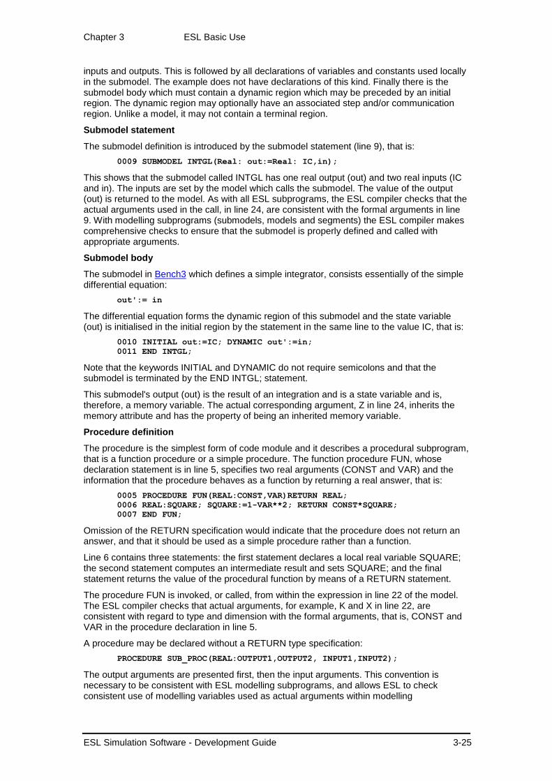
Chapter 3 ESL Basic Use
ESL Simulation Software - Development Guide 3-25
inputs and outputs. This is followed by all declarations of variables and constants used locally in the submodel. The example does not have declarations of this kind. Finally there is the submodel body which must contain a dynamic region which may be preceded by an initial region. The dynamic region may optionally have an associated step and/or communication region. Unlike a model, it may not contain a terminal region.
Submodel statement
The submodel definition is introduced by the submodel statement (line 9), that is:
0009 SUBMODEL INTGL(Real: out:=Real: IC,in);
This shows that the submodel called INTGL has one real output (out) and two real inputs (IC and in). The inputs are set by the model which calls the submodel. The value of the output (out) is returned to the model. As with all ESL subprograms, the ESL compiler checks that the actual arguments used in the call, in line 24, are consistent with the formal arguments in line 9. With modelling subprograms (submodels, models and segments) the ESL compiler makes comprehensive checks to ensure that the submodel is properly defined and called with appropriate arguments.
Submodel body
The submodel in Bench3 which defines a simple integrator, consists essentially of the simple differential equation:
out':= in
The differential equation forms the dynamic region of this submodel and the state variable (out) is initialised in the initial region by the statement in the same line to the value IC, that is:
0010 INITIAL out:=IC; DYNAMIC out':=in;
0011 END INTGL;
Note that the keywords INITIAL and DYNAMIC do not require semicolons and that the submodel is terminated by the END INTGL; statement.
This submodel's output (out) is the result of an integration and is a state variable and is, therefore, a memory variable. The actual corresponding argument, Z in line 24, inherits the memory attribute and has the property of being an inherited memory variable.
Procedure definition
The procedure is the simplest form of code module and it describes a procedural subprogram, that is a function procedure or a simple procedure. The function procedure FUN, whose declaration statement is in line 5, specifies two real arguments (CONST and VAR) and the information that the procedure behaves as a function by returning a real answer, that is:
0005 PROCEDURE FUN(REAL:CONST,VAR)RETURN REAL;
0006 REAL:SQUARE; SQUARE:=1-VAR**2; RETURN CONST*SQUARE;
0007 END FUN;
Omission of the RETURN specification would indicate that the procedure does not return an answer, and that it should be used as a simple procedure rather than a function.
Line 6 contains three statements: the first statement declares a local real variable SQUARE; the second statement computes an intermediate result and sets SQUARE; and the final statement returns the value of the procedural function by means of a RETURN statement.
The procedure FUN is invoked, or called, from within the expression in line 22 of the model. The ESL compiler checks that actual arguments, for example, K and X in line 22, are consistent with regard to type and dimension with the formal arguments, that is, CONST and VAR in the procedure declaration in line 5.
A procedure may be declared without a RETURN type specification:
PROCEDURE SUB_PROC(REAL:OUTPUT1,OUTPUT2, INPUT1,INPUT2);
The output arguments are presented first, then the input arguments. This convention is necessary to be consistent with ESL modelling subprograms, and allows ESL to check consistent use of modelling variables used as actual arguments within modelling

Chapter 3 ESL Basic Use
ESL Simulation Software - Development Guide 3-26
subprograms. A non-function procedure may only be called from a procedural code region, for example:
SUB_PROC(O1,O2 := I1,I2);
ESL checks that the actual output arguments (O1 and O2 in this case) are variables (not expressions), and that they can accept new values returned from the called procedure. Any actual arguments which appear before the ":=" symbol must be capable of accepting a returned value, that is variables, subscripted variables, arrays or array slices, but not expressions. Arguments appearing after the ":=" sign are not restricted and may be expressions.
ESL does not check that the procedure definition uses its formal arguments in the manner indicated by the call (that is as output or input). It is the user's responsibility to be consistent in the procedure definition and the call.
If no ":=" appears in the calling argument list, all arguments are regarded as outputs, and may not be expressions. Alternatively if the assignment symbol appears before the first argument, for example:
SUB_PROC(:=x1,x2,x3,x4);
all arguments are treated as inputs.
Arguments of function procedures are treated as inputs.
Note that local data variables retain their values between calls of the procedure, consider:
REAL: SQUARE /0.0/;
The initialisation of SQUARE with the value 0.0 occurs once only at the start of program execution. If SQUARE is changed in a call to the procedure, it will have its most recent value available in the next call to the procedure. In modelling subprograms the initialisation process occurs at the start of every simulation run, not just at the start of the program.
Standard functions (Procedures)
The following standard functions are part of the ESL language and are implicitly declared:
SIN sine of argument (radians)
ASIN arc-sine of argument
COS cosine of argument (radians)
ACOS arc-cosine of argument
ATAN arc-tangent of argument
ATAN2 arc-tangent of two arguments
LOG natural logarithm of argument
EXP exponential of argument
ABS absolute value of argument
SQRT square root of argument
RAND pseudo-random number
INT integer value of argument
LEN returns total number of array elements
LEN_1 number of elements in first dimension of array
LEN_2 number of elements in second dimension of array
LEN_3 number of elements in third dimension of array
ACHAR character value corresponding to ASCII code
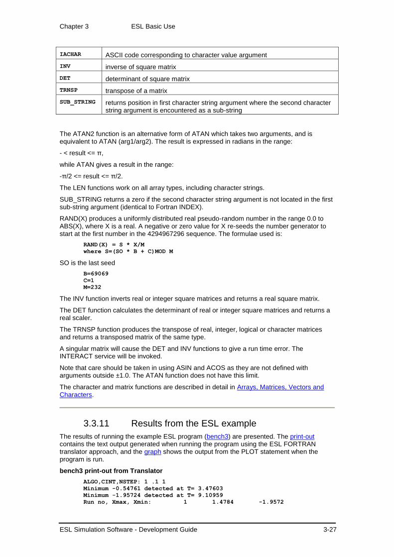
Chapter 3 ESL Basic Use
ESL Simulation Software - Development Guide 3-27
IACHAR ASCII code corresponding to character value argument
INV inverse of square matrix
DET determinant of square matrix
TRNSP transpose of a matrix
SUB_STRING returns position in first character string argument where the second character string argument is encountered as a sub-string
The ATAN2 function is an alternative form of ATAN which takes two arguments, and is equivalent to ATAN (arg1/arg2). The result is expressed in radians in the range:
- < result <= π,
while ATAN gives a result in the range:
-π/2 <= result <= π/2.
The LEN functions work on all array types, including character strings.
SUB_STRING returns a zero if the second character string argument is not located in the first sub-string argument (identical to Fortran INDEX).
RAND(X) produces a uniformly distributed real pseudo-random number in the range 0.0 to ABS(X), where X is a real. A negative or zero value for X re-seeds the number generator to start at the first number in the 4294967296 sequence. The formulae used is:
RAND(X) = S * X/M
where S=(SO * B + C)MOD M
SO is the last seed
B=69069
C=1
M=232
The INV function inverts real or integer square matrices and returns a real square matrix.
The DET function calculates the determinant of real or integer square matrices and returns a real scaler.
The TRNSP function produces the transpose of real, integer, logical or character matrices and returns a transposed matrix of the same type.
A singular matrix will cause the DET and INV functions to give a run time error. The INTERACT service will be invoked.
Note that care should be taken in using ASIN and ACOS as they are not defined with arguments outside ±1.0. The ATAN function does not have this limit.
The character and matrix functions are described in detail in Arrays, Matrices, Vectors and Characters.
3.3.11 Results from the ESL example
The results of running the example ESL program (bench3) are presented. The print-out contains the text output generated when running the program using the ESL FORTRAN translator approach, and the graph shows the output from the PLOT statement when the program is run.
bench3 print-out from Translator
ALGO,CINT,NSTEP: 1 .1 1
Minimum -0.54761 detected at T= 3.47603
Minimum -1.95724 detected at T= 9.10959
Run no, Xmax, Xmin: 1 1.4784 -1.9572

Chapter 3 ESL Basic Use
ESL Simulation Software - Development Guide 3-28
Minimum -1.07265 detected at T= 3.34763
Minimum -2.01486 detected at T= 9.14304
Run no, Xmax, Xmin: 2 1.9264 -2.0149
Minimum -1.36838 detected at T= 2.91687
Minimum -2.01989 detected at T= 9.17648
Run no,Xmax, Xmin: 3 2.0069 -2.0199
Minimum -1.50791 detected at T= 2.55872
Minimum -2.02236 detected at T= 9.30282
Run no, Xmax, Xmin: 4 2.0206 -2.0224
Minimum -1.58431 detected at T= 2.28501
Minimum -2.02330 detected at T= 9.54240
Run no, Xmax, Xmin: 5 2.0231 -2.0233
RUN NO. K XMAX
1 1.0000 1.4784
2 1.5000 1.9264
3 2.0000 2.0069
4 2.5000 2.0206
5 3.0000 2.0231
Graph generated by PLOT statement when program run

Chapter 4 ESL Operation and Program Structure
ESL Simulation Software - Development Guide 4-1
CHAPTER 4
4 ESL Operation and Program Structure
This section describes the structure of the ESL language, its operation and fundamental principles.
Contents:
ESL Program Types
ESL Program Structures
Procedural Program Structure
Modelling Subprogram Structure
Variables - Scope, Type and Usage
The Simulation Process
4.1 ESL Program Types ESL supports a number of functionally different program types:
ESL STUDY: a conventional ESL simulation program with an Experiment which calls a model and its subprograms.
ESL REMOTE: defines an ESL modelling segment which is to be executed on a separate processor as part of a distributed simulation.
ESL EMBEDDED: defines an ESL modelling segment which is to be embedded in, and called from, a FORTRAN or C++ main program.
ESL non program: allows the user to "check" compile ESL source code without producing a .hcd file.
Using these different program types users may develop simulations which run as a single process, or as several processes executing on a distributed network of computers.
4.1.1 The ESL STUDY
The ESL STUDY is a basic ESL simulation program that begins with the keyword STUDY and must end with the keyword END_STUDY. All of the program components shown in the below may be included.

Chapter 4 ESL Operation and Program Structure
ESL Simulation Software - Development Guide 4-2
ESL Program Structures
Within a basic STUDY there are two main sections, the "System Definition" and the "Experiment". The System Definition describes the requirements of the simulation, both statically and dynamically, whereas the Experiment describes the procedural operations which control the simulation runs. The system definition, (which is divided into separate modules such as MODEL, SUBMODEL etc.), and the Experiment can both be regarded as individual modules for the purposes of compilation. The main task of the Experiment is to define the simulation runs to be performed, and possibly set parameter values to control the run (alternatively such parameters may be set in the MODEL INITIAL region). The Experiment calls one or more Models (sequentially), which in turn call other subprograms. Modules must be declared before they are used and for this reason the Experiment is placed at the end of the ESL STUDY.
4.1.2 The ESL REMOTE program
The REMOTE program defines an ESL segment (part of the system being modelled) which is to be executed as a remote process, either on the same processor, or on a different processor on a computer network. It is identified with the keyword REMOTE (no end keyword), and may include PROCEDUREs, PACKAGEs, SUBMODELs, and one, and only one, SEGMENT. It extends the concurrent processing concept of segments into true distributed simulation. ESL Segments describes how SEGMENTS are used.
4.1.3 The ESL EMBEDDED program
The EMBEDDED program defines an ESL segment (representing the system being modelled) which is to be called from a FORTRAN or C++ main program. It is identified with the keyword EMBEDDED (no end keyword), and like the REMOTE program may include PROCEDUREs, PACKAGEs, SUBMODELs, and one SEGMENT. The EMBEDDED program is fully described in ESL Segments which examines SEGMENTS in detail.

Chapter 4 ESL Operation and Program Structure
ESL Simulation Software - Development Guide 4-3
4.1.4 The ESL non program
A "non-program" is a fragment of ESL code which does not itself constitute a complete program. For example, it could be a SUBMODEL, PROCEDURE or PACKAGE which is to be inserted into an ESL program using the INCLUDE statement. Any file which does not start with the keyword STUDY, or REMOTE or EMBEDDED, is a non-program and can be checked with the compiler without producing a .hcd file.
When writing a SUBMODEL, or function (PROCEDURE), for use as an ISE simulation element, this should be regarded as a non-program and compiler checked before importing into ISE. The points to note with ISE text subprograms are:
The file must have a .esl extension.
The file-name must match the SUBMODEL, or function PROCEDURE, name.
4.2 ESL Program Structures The basic ESL program structure identifies the six basic modules of an ESL program:
Data definition PACKAGE.
Procedural (non-modelling) subprogram - PROCEDURE.
Modelling subprogram - SUBMODEL.
Parallel modelling subprogram - SEGMENT.
Model subprogram - MODEL.
Simulation procedural EXPERIMENT.
Not all the modules making up a program need be contained within a single .esl file. Other files in the current directory or the ESL library directory, or indeed in any directory with an appropriate path definition may be introduced with the INCLUDE statement.
To the above list can be added the EXTERNAL procedures, which are expressed in another language such as FORTRAN, C or C++, and are also stored in separate files.
These program modules are described in detail in the following sections, but first ESL data-types and their declarations are considered.
4.2.1 ESL data types
Each ESL module has an associated local data set, which is accessed by named variables declared within the module. Note SUBMODELs have separate local data sets for each invocation. Strict rules apply to communicating data between modules, which may only by achieved through subprogram arguments, or by means of the ESL PACKAGE mechanisms.
ESL supports the four basic data types, that is: REAL floating point numbers, which may have both a whole number and fraction parts; INTEGER numbers or whole numbers; LOGICAL data only having the values TRUE or FALSE; and CHARACTER data. Arrays of up to three dimensions may be specified for each of the basic data types.
Type declarations
Four basic type keywords are used to declare variables in ESL:
REAL
INTEGER
LOGICAL
CHARACTER
All variables must be declared prior to use (with the exception of the RESERVED variables). Once declared, a variable may not be re-declared within its scope, although a variable with the same name may be declared locally in another subprogram without conflict. The declaration may optionally include an initialisation of that variable, for example:
Chapter 4 ESL Operation and Program Structure
ESL Simulation Software - Development Guide 4-4
REAL:alpha,beta/4.6/;
INTEGER:count/0/;
LOGICAL:flag/true/;
CHARACTER:message(18)/"This is a message!"/;
Any of the basic types may be declared as one, two or three dimensional arrays by including the size of each dimension in parenthesis after the variable name. In the example above, the character variable message is a one dimensional array of 18 elements. For character declarations, the literal string must exactly match the array size. See Arrays, Matrices, Vectors and Characters for detailed specification of array declaration and use.
The values given to variables must match their declared type. A REAL set to 0 or INTEGER set to 0.0 will cause an error message, and compilation failure. A logical must be set to either TRUE or FALSE which may not be abbreviated.
Constants are declared by preceding the above declarations by the keywords CONSTANT or PARAMETER. Values of constants may not be changed from that given in the declaration. Parameters are similar to constants, but they may be changed "externally" by a simulation driver file (see ESL Run Control) or via ISE (see Variables Window).
Non-variable declarations
Besides declarations of data variables, a module's local declaration section may also specify access to ESL PACKAGE data by means of a USE declaration, for example:
USE PACK_NAME;
In addition external non-ESL coded procedures (for example, FORTRAN or C) may be called from a module provided they are declared by an EXTERNAL declaration.
4.2.2 The ESL experiment
This is the default region of an ESL study. Any section of code not defined as a subprogram or data package is termed the experiment. It is procedural, meaning the code is executed in the order in which it is presented. A STUDY comprising only the experiment is valid and may be compiled and run. The experiment region is always the last part of the STUDY - the comment "-- EXPERIMENT" is helpful to identify this region but is not mandatory. The experiment may only call MODELs or PROCEDUREs, in sequence. The experiment is used to specify simulation runs by calling one, or more, MODELs. It may also be used to set parameters which control each simulation run, for example, simulation start time, finish time, integration algorithm etc.
Alternatively this function may be undertaken by the MODEL INITIAL region.
4.2.3 The ESL MODEL
The MODEL is the main "simulation module" of an ESL program. Any number of separate MODELs may exist but only one may be active at one time. A detailed description of a MODEL body, and other modelling subprograms, is given in Modelling Subprogram Structure.
A MODEL is declared by the keyword MODEL, followed by the model name, which may be followed by a list of arguments in parenthesis, or empty parenthesis, or no parenthesis at all. In each case the declaration is terminated with a semi-colon, ";". For example:
MODEL model_name (REAL:variable1:=REAL:variable2);
MODEL model_name ();
MODEL model_name;
The name may be any length up to the end of a full line (132 characters), but only the first 28 characters will be recognised.
The MODEL arguments must match the actual, or calling arguments, with respect to number and type. Note the use of the ":=" token in the above example, which distinguishes between the output arguments, which come first, and the input arguments, which follow. If this token is omitted, all arguments will be assumed to be outputs. A type declaration may be followed by any number of argument names of that type, separated by a comma. Where a new type declaration is required, then a semi-colon, ";", is used as a separator.

Chapter 4 ESL Operation and Program Structure
ESL Simulation Software - Development Guide 4-5
MODEL model_name (REAL:variable1,variable2;INTEGER:ivar1,
ivar2,ivar3:=REAL:variable3,variable4;
INTEGER:ivar4;FILE:record);
In the above example, two real and three integer output arguments are defined, with two real, one integer and a file specifier input argument. Note that statements may be continued on subsequent lines. The end of line must not, however, appear within an identifier, text string, or number. All ESL data types are permitted in the argument list, although for a MODEL, or SEGMENT, arrays must have explicit dimensions (not implicit "*" dimensions which are permitted in all other ESL subprograms).
The MODEL may only be called from the experiment and will take the form shown below:
model_name (out1,out2,out3,out4,out5:=in1,in2,in3,filename);
where the argument list must match the MODEL declaration in terms of number, order and type. The position of the ":=" symbol which identifies the output and input arguments must also match in the call and declaration. Output arguments must be variables, but the input arguments may be variables, constants, numbers or expressions of the appropriate type.
The MODEL must be terminated with an END statement which may optionally include the MODEL name. If the name is included however, the compiler will check that it is correct and issue an error if not.
4.2.4 The ESL SUBMODEL
The SUBMODEL provides one method of allowing a simulation to be divided into functional areas or modules. It is similar to the MODEL except that it may only be called from the DYNAMIC region of a MODEL, SEGMENT or another SUBMODEL. A SUBMODEL call is classed as modelling, or non-procedural code. This means that several invocations of the same SUBMODEL may exist simultaneously, called from different sections of modelling code regions. Each invocation of a submodel is associated with separate submodel data storage. For example, the variable X locally declared in a submodel, has different storage associated with X for each separate invocation of the submodel. Note however that the SUBMODEL is not recursive - it cannot be called, directly or indirectly, from its own DYNAMIC region.
With the exception of the TERMINAL and ANALYSIS regions, which are not permitted in a SUBMODEL, the internal structure is the same as the MODEL.
The declaration of a SUBMODEL is similar to that of the MODEL, but consider the simple limit submodel:
SUBMODEL LIMIT(REAL:y := CONSTANT REAL:LL,UL; REAL:x);
REAL: range,xnorm;
INITIAL
range:= UL-LL;
DYNAMIC
xnorm:= (x-LL)/range;
y:= if xnorm > 1.0 then UL
else_if xnorm < 0.0 then LL
else x;
END LIMIT;
Here the input arguments LL and UL are declared to be CONSTANT, which means that their values will be taken to be the same throughout the simulation run. ESL exploits this knowledge and produces faster, optimised code, by only passing the CONSTANT arguments to the SUBMODEL once at the start of a simulation run, and not every time the value of the limited output is required. Although CONSTANT input arguments may be specified for MODELs and SEGMENTs ESL currently takes no special action.
Unlike a MODEL, a SUBMODEL allows the implicit dimensions in array arguments, for example, ARRAY(*,*).
The SUBMODEL call, however, is very different to that of the MODEL, that is:
out1,out2:=submodel_name(in1,in2,in3);

Chapter 4 ESL Operation and Program Structure
ESL Simulation Software - Development Guide 4-6
The call is an assignment with the output arguments appearing as variables to the left of the assignment symbol, ":=", (the order of course must be the same as in the declaration). Input arguments are given in parenthesis. SUBMODELs without arguments, or with input arguments only, would be called as:
No_args_submodel;
another_no_args();
no_output_args_submodel(in1,in2);
The SUBMODEL call is a complete statement and cannot be embedded as part of an expression. Like the MODEL call arguments, actual arguments must match formal arguments, but the "*" symbol may be used to dimension arguments arrays where the array dimension is defined by the actual argument.
4.2.5 The ESL SEGMENT
A third type of modelling subprogram is the SEGMENT which is almost identical to and runs in parallel with the main MODEL. Its operation can either be as:
Emulated parallel processing: that is running in the same process as the MODEL and included within the same STUDY.
Remote parallel processing: running as a separate process on the same or different processor to the MODEL (for example, over a network).
As an embedded simulation running under the control of a program other than the ESL MODEL, for example, a C++ program.
These options are discussed in ESL Segments, and the basic model-segment relationship is illustrated in below.
Model - Segment Linking
The structure of a SEGMENT is identical to that of a MODEL except that no TERMINAL or ANALYSIS region is permitted. The declaration has the form:
SEGMENT parallel_seg(REAL:invar:=REAL:outvar);
or
SEGMENT parallel_seg(REAL:invar:=REAL:outvar) EXTERNAL;
The second form of declaration means that the SEGMENT is to be executed remotely in a separate process. Note all the following code until after the corresponding END statement is ignored if EXTERNAL is appended to the declaration.
An emulated SEGMENT may only be called from one place, the COMMUNICATION region of a MODEL.
A remote SEGMENT may be called from the COMMUNICATION region of either a MODEL or an embedded SEGMENT.

Chapter 4 ESL Operation and Program Structure
ESL Simulation Software - Development Guide 4-7
The form of a segment call is:
parallel_seg(svar1:=svar2);
Note that the call may be conditional, that is the subject of an IF statement. Any number of SEGMENTs may be specified and run simultaneously. The call to the SEGMENT in the COMMUNICATION region basically has the task of receiving the output argument values from the SEGMENT following the SEGMENT's solution of the last communication interval. After the MODEL's COMMUNICATION region has been executed (and a SEGMENT call made), the SEGMENT input arguments are passed to the SEGMENT, and it is instructed to solve the next communication interval. An exception to this basic calling pattern is the first call to a SEGMENT in a run. In this case the input arguments are passed to the SEGMENT during the COMMUNICATION region call, to enable the SEGMENT to perform its initialisation and return values for its initial output arguments.
4.2.6 The ESL PROCEDURE
There are two types of PROCEDURE, procedures and functions, which are non-modelling subprograms. Both contain procedural code, and are identified by the keyword PROCEDURE; functions being distinguished by a declared RETURN type. Procedures may be called from any procedural code region (including a procedural block, or WHEN body, in the DYNAMIC region of a modelling subprogram, but not directly from a DYNAMIC region). Functions, however, may be called from expressions appearing in any region. Their primary purpose is for non-modelling, or procedural, programming, however they may play an important part in the simulation specification.
4.2.7 The ESL PACKAGE
The PACKAGE provides an means of accessing the same data from different subprograms. Once data in a PACKAGE has been declared, it may be accessed by any subprogram specifically requesting access to that PACKAGE.
A PACKAGE is declared after the STUDY keyword and before modules where it is required, for example:
PACKAGE users_data;
REAL:var1,var2,var3;
INTEGER:ivar1/2/,ivar2/3/;
CONSTANT INTEGER:ivar3/4/;
CHARACTER: char1,char2;
END users_data;
Note that the optional initialisation of variables, except for the CONSTANT, which must be initialised.
Subprograms which wish to access the PACKAGE data must include the following declaration:
USE users_data;
This provides access to all the variables declared in the PACKAGE users_data.
Note that variables declared in a PACKAGE are of a class referred to as "procedural variables" which restricts their use in modelling subprograms, see Variables - Scope, Type and Usage.
PACKAGES are also a means by which ESL is able to share data with program code expressed in other languages, for example, FORTRAN or C routines called as EXTERNALs (see External Procedures). The package data may be exactly mapped on to a named FORTRAN COMMON block.
RESERVED package
A special RESERVED PACKAGE, is defined which contains variables to control the simulation process. These variables are specified in ESL Basic Use (see Reserved PACKAGE).

Chapter 4 ESL Operation and Program Structure
ESL Simulation Software - Development Guide 4-8
Certain reserved variables may be changed prior to a MODEL call to define a simulation run, or in fact in the MODEL INITIAL region. Access to the RESERVED variables is implicit in all subprograms except procedures and functions which must include the statement:
USE RESERVED;
to gain access.
4.3 Procedural Subprogram Structure The two types of PROCEDURE, that is procedures and functions, are non-modelling subprograms. They contain procedural code, and their primary purpose is for non-modelling, or procedural, programming, however they may play a part in the simulation specification.
Procedures
With a procedure subprogram formal arguments are declared within parenthesis in the normal way, except that no distinction is made between inputs and outputs (the ":=" symbol is not used). The compiler makes no checks on the actual use to which the variables are put. For example, consider the declaration:
PROCEDURE proc_name (REAL:output,input1,input2);
Each formal argument could be either input or output, but in this case we assume the first argument is output (it is set or changed in the procedure), and the remaining arguments inputs. The PROCEDURE could be called with the statement:
proc_name (alpha_output := beta_input * factor, gamma_input);
Since the first formal argument is an output argument then the corresponding actual argument must be a variable, for example, alpha_output, which can receive a value returned from the procedure. The input arguments may be expressions or numbers, for example, beta_input * factor, or variables, for example, gamma_input. It is erroneous to use an expression for an actual argument when the corresponding formal argument is classed as output. ESL does not apply the same rigid checks on procedural code as for the modelling modules, and does not check that the procedure uses the actual arguments in the manner indicated by the call, that is, as output or input.
Functions
Functions return a single value specified by a RETURN variable type following the declaration:
PROCEDURE fun_name(REAL:theta,phi) RETURN REAL;
The formal arguments in parenthesis are inputs by default, and a single value of the type indicated is returned. The body of the function must include a RETURN statement as the last statement of the function, followed by a variable or expression of the type indicated in the declaration:
PROCEDURE sumsquare(REAL:theta,phi) RETURN REAL;
REAL:outvar;
outvar:=(theta+phi)**2;
RETURN outvar;
END sumsquare;
alternatively, the function body could consist the single statement:
RETURN (theta+phi)**2;
ESL allows additional RETURN statements to be included to indicate alternative exit points from the function, but the last statement MUST be a RETURN. Functions may also return arrays or character strings providing the returned type corresponds to that declared.
Calling a function PROCEDURE is also different in that it is called from an expression, and may be considered as a single value in that expression. For example:
a:= alpha + sumsquare(b,c) * d;

Chapter 4 ESL Operation and Program Structure
ESL Simulation Software - Development Guide 4-9
will substitute the returned value in the expression. Functions used in this way may be included in modelling code expressions in the DYNAMIC region.
Also note that ESL treats the arguments of the function as inputs, which should not be changed by the function definition.
Standard functions
ESL includes a number of standard functions which may be used, without declarations, in any expression. These are listed in ESL Basic Use (see Standard functions).
External procedures
Both functions and procedures may be written in another language, for example, FORTRAN, C, or C++ and be called in the same way as "internal" ESL PROCEDURES. External FORTRAN or C modules may be called from an ESL program that has been translated to FORTRAN (esl -tf). External C++ modules may only be called from a C++ translated program (esl -tcc). To satisfy the ESL requirement that all modules are declared before use the EXTERNAL keyword is used in one of two ways.
For external FORTRAN or C procedures, an external statement must be placed in the declarative region of the subprogram that calls the external procedure, for example:
EXTERNAL EXTSUB;
EXTERNAL REAL: EXTFUN;
In this example EXTSUB may be called as an ESL PROCEDURE, but unlike an internal procedure ESL cannot check if the arguments are of the correct type, or whether there are the correct number of arguments. The EXTERNAL function PROCEDURE is assumed to return a REAL value, but no other assumptions are made. The two external procedures could be called by:
EXTSUB(a := b*c, d);
x:= EXTFUN(y, z*z) * a;
The argument passing conventions between ESL and other languages are specified in External Procedures, and this section describes the use of PACKAGE data by non-ESL routines.
An alternative method, which allows more extensive checking for consistent use of externals, and is mandatory for the C++ Translator is described below.
The form of the declaration is similar to the declarative statement used for an ESL procedure, or procedure function. For example:
procedure ext_proc(real: r; integer: i, j; real:arr(*))EXTERNAL;
This declarative statement must appear in the same position as an equivalent ESL procedure. That is, after the STUDY statement, and prior to the module where it is first used.
External function procedures are defined in a similar manner, for example:
procedure ext_fun(real: x) return real EXTERNAL;
procedure ext_int_fun(real: x) return integer external;

Chapter 4 ESL Operation and Program Structure
ESL Simulation Software - Development Guide 4-10
4.4 Modelling Subprogram Structure This section describes the basic structure of the ESL Modelling Subprograms, (MODEL, SUBMODEL and SEGMENT). Code in ESL Modelling Subprograms is represented in two distinct ways. That is the procedural parts in which the order of calculation is exactly specified, and the dynamic part which represents parallel, concurrent, simulation of the modelled system components. The sequential, more conventional code is termed "procedural code" and the dynamic part "modelling code".
4.4.1 Modelling code
Modelling code is restricted exclusively to the DYNAMIC regions of MODELs, SUBMODELs and SEGMENTs. These regions may only contain modelling code, with two exceptions: procedural code may be used in a WHEN block, or in a PROCEDURAL block.
Modelling code comprises:
Assignment statements, which include differential and transfer function specifications, and the use of an IF-clause.
SUBMODEL calls.
WHEN statements, for detecting event discontinuities.
PROCEDURAL blocks, for including procedural code.
ESL also restricts the variables that can be directly set in the DYNAMIC region to algebraic variables only, see Variables - Scope, Type and Usage.
4.4.2 Procedural code
Any code that executes in the sequential order in which it is written is termed procedural code. In ESL this comprises all statements such as loops, PROCEDURE calls, file operations and general expression assignments. The only way to use procedural code in a DYNAMIC region is in the body of a PROCEDURAL block or the body of a WHEN statement block.
The WHEN statement block
The WHEN statement allows "events" to be detected, at which time the body of the WHEN block is executed. For example:
WHEN T >= 8.125 THEN
Y:= 0.0;
END_WHEN;
This treats the WHEN trigger condition T >= 8.125 as a discontinuity. ESL accurately detects "when" the condition becomes TRUE, and at that point, and only that point, is the body of the WHEN statement executed. See Modelling Code for a full discussion of the WHEN statement, and discontinuities.
The PROCEDURAL block
The difference between modelling and procedural code is quite clear, and separation between the two code forms is rigidly enforced. There are occasions however when it is necessary to perform some procedural operations in the modelling code (DYNAMIC) region, for example, setting individual array elements. To allow for this ESL provides the PROCEDURAL block which is treated as a single modelling code statement which contains procedural code statements. Variables local to the subprogram in which the block is placed may be used within the block. It is necessary - to ensure correct variable usage - to place any variables used in both the subprogram and in the block in an argument list after the block declaration. This ensures that ESL will then sort the block as appropriate in the DYNAMIC region as it does any other statement referencing these variables. The normal input and output conventions with argument lists is observed.
The following example shows the setting of individual matrix elements (one of the few occasions it is appropriate to use a PROCEDURAL block):

Chapter 4 ESL Operation and Program Structure
ESL Simulation Software - Development Guide 4-11
DYNAMIC
....
B:=A*2;
PROCEDURAL (A:=x,y,z);
A(1,1):=x;
A(2,1):=y;
A(1,2):=z;
END_PROCEDURAL;
....
The array, A, is an output and the variables, x, y, z, are inputs. The whole block is sorted, as a single entity, along with other modelling code statements into an appropriate execution order. In this example this means the PROCEDURAL block is executed before the assignment to B is performed.
Any number of PROCEDURAL blocks may be used in any of the Modelling Subprograms.
As a general rule, PROCEDURAL blocks should only be used where absolutely necessary, and in the prescribed way with proper inputs and outputs. They should not be used as a means of bypassing ESL's strict variable usage checks.
4.4.3 Modelling subprogram regions
Modelling subprograms are divided into a number of distinct code regions, each region having a particular function in the simulation process.
Declarations
A modelling subprogram starts with the declaration of the subprogram, which is followed by local declarations required by the subprogram code. All variables used in the subprogram must be declared. The scope of a locally declared variable does not extend to other subprograms unless explicitly passed as an argument. Variables declared outside the subprogram in PACKAGEs must also be explicitly declared by means of the USE package statement which references all variables in that PACKAGE. (This does not apply to RESERVED variables which are a special case and do not need declaring - except in PROCEDURES.)
A variable may be declared by a "type" keyword followed by a colon and then the variable name(s), for example:
REAL:alpha,beta(2,2);
INTEGER:gamma,theta;
LOGICAL:flag1,flag2;
CHARACTER:string1(20);
FILE:record;
Type declarations may optionally include initial values, for example:
REAL:alpha/3.3/,beta/4.4/;
These variables are initialised at the start of each simulation run.
Data values are mandatory if declaring a constant or parameter:
CONSTANT REAL:pi/3.14159/;
PARAMETER INTEGER:n1/5/;
INITIAL region
The INITIAL region is introduced with the keyword INITIAL, see Basic MODEL Structure, and it is used to initialise variables, or to carry out any necessary calculations, prior to starting the simulation run. It may also set values of RESERVED variables to control the simulation run. The INITIAL region is optional, and if it is used it must precede the DYNAMIC region. Initialisation for certain types of variables, that is, "state variables" must be performed prior to entering the DYNAMIC code region.

Chapter 4 ESL Operation and Program Structure
ESL Simulation Software - Development Guide 4-12
Basic MODEL Structure
MODEL model_name();
-- declarations
...
...
INITIAL
-- procedural code (initial variable values)
...
...
DYNAMIC
-- modelling code
...
...
STEP
-- procedural code (executed after each integration step)
...
...
COMMUNICATION
-- procedural code (executed after each comm. period)
...
...
TERMINAL
-- procedural code (executed at end of simulation run)
...
...
ANALYSIS
-- procedural code (for steady-state analysis)
...
...
END model_name;
DYNAMIC region
The DYNAMIC region is mandatory for all modelling subprograms, and is where the modelling code is placed. It is introduced by the keyword DYNAMIC and may optionally be followed by the STEP, COMMUNICATION, TERMINAL and ANALYSIS regions. The region may be empty, but the keyword DYNAMIC must appear in every modelling subprogram.
STEP region
The STEP region, which is introduced by the keyword STEP, and logically is part of the DYNAMIC region, is used for procedural code and is executed at certain points in the simulation, after each integration step. It is optional in MODELs, SUBMODELs and SEGMENTs, and if used must immediately follow the DYNAMIC region.
COMMUNICATION region
The COMMUNICATION region, which is introduced by the keyword COMMUNICATION, and logically is also part of the DYNAMIC region, is procedural code executed at precise points during the simulation run (after each communication interval, CINT). It is optional, and if used it must follow the DYNAMIC region and any STEP region.
TERMINAL region
The TERMINAL region, introduced by the keyword TERMINAL, is used to execute procedural code when the simulation run is completed. This occurs either when the simulation time T reaches TFIN, or the statement TERMINATE is activated. The statements in the TERMINAL region will be executed immediately before returning to the experiment. It may only appear in a MODEL subprogram, where it is optional, and if used must follow the COMMUNICATION or STEP regions.
ANALYSIS region
The ANALYSIS region of the MODEL is a procedural code region introduced by the keyword ANALYSIS. It is executed only on special MODEL calls from the experiment (ALGO set to LIN1 or LIN2), and is used to undertake steady-state analysis and linearization. It may only appear in a MODEL, where it is optional, and then it must be the last region of the MODEL. The ANALYSIS region is fully described in Steady-State Analysis.

Chapter 4 ESL Operation and Program Structure
ESL Simulation Software - Development Guide 4-13
4.5 Variables - scope, type and usage ESL is unlike a general-purpose programming language, in that the program features special modules (experiment, MODEL, SUBMODEL, SEGMENT), which have a specific structure to address the special requirements of simulation. The way in which it treats user declared variables is also different.
The first point to note is that the scope of a variable is restricted to the section of program in which it is declared (experiment, MODEL, SUBMODEL, SEGMENT or procedural subprogram), that is, it is local to a module. It can be used in other modules if it is passed in an argument list (for example, in a call to a MODEL or SUBMODEL), or if it is included in a PACKAGE declaration, in which case it is common to all subprograms specifically requesting access, by a USE declaration. All actual and formal arguments to subprograms must be of the same type and with matching dimensions. The ESL compiler checks these points and generates error messages where appropriate.
ESL is also different from general-purpose programming languages in the way in which the ESL compiler treats variables according to their "class". The class is a property which the ESL compiler gives to each variable, on the basis of how that variable is used. The following classes, and sub-classes are used:
Model variables.
Procedural variables.
Constants.
ESL Parameters.
Model variables comprise:
Memory variables.
Algebraic variables.
Inherited class variables.
Memory variables comprise:
model parameters.
State variables.
The following describes each class of variable in turn.
4.5.1 Model parameters
Model parameters (sub-class of memory variables) are declared in modelling subprograms (MODELs, SUBMODELs or SEGMENTs), as local variables, or as an output argument of the modelling subprogram. They are variables which are used in the DYNAMIC region, but have a constant value during an integration step, or for longer periods. That is, as far as the integration process is concerned these variables are constant, and their value does not depend on current conditions. The derivation of model parameters is illustrated in the figure below.

Chapter 4 ESL Operation and Program Structure
ESL Simulation Software - Development Guide 4-14
Algebraic Variables and Model Parameters
The local declaration may include an initial value, or an INITIAL region assignment statement may be used to give these variables an initial value. Model parameters, generally, once set are intended to remain fixed throughout a period of the simulation, and are treated as constants by the integration algorithm. Modification is however possible in procedural code regions such as the STEP and COMMUNICATION regions, or in the body of a WHEN or PROCEDURAL block in the DYNAMIC region. If set in a WHEN block, the variable will be updated at the instant the WHEN triggers, and subsequently the simulation (integration) will see a new constant value. Note that the body of a WHEN statement is executed between integration steps, effectively as part of the STEP region, and not as part of the DYNAMIC region.
Failure to give an initial value to model parameter will result in an error message.

Chapter 4 ESL Operation and Program Structure
ESL Simulation Software - Development Guide 4-15
The following example shows two model parameters, tau and limit.
SUBMODEL SUB(REAL: y := REAL: x);
REAL: tau/1.0/,limit;
INITIAL
limit:=10.0;
y:=0.0;
DYNAMIC
y':= (x-y)/tau;
when y >= limit then
tau:=1.5;
when y < limit then
tau:=1.0;
end_when;
COMMUNICATION
if t > 8.125 then
limit:=12.0;
end_if;
END SUB;
The variable tau is initialised in the declaration, and only changes value in the event of the WHEN statement triggering. The body of a WHEN statement is executed between integration steps, at the point detected as the WHEN trigger point.
The variable limit is given an initial value, in the INITIAL region, and then only changed in the COMMUNICATION region, between integration steps, when t exceeds 8.125.
4.5.2 State variables
State variables (sub-class of memory variables) are declared in modelling subprograms (MODELs, SUBMODELs or SEGMENTs), as local variables, or as an output argument of the modelling subprogram. They are identified by ESL when differential equations are defined in the DYNAMIC region, this is illustrated in the figure below. Each state variable is coupled with a corresponding derivative algebraic variable. This means for differential equations of higher than first order, more than one state variable will exist, for example:

Chapter 4 ESL Operation and Program Structure
ESL Simulation Software - Development Guide 4-16
Derivation and use of State Variables
Algebraic variable derivatives Corresponding state variables
x' := x
y'' := y', y
z''' := z'', z', z
The state variable value is produced as a result of integration (solving the differential equation). Its current value depends on the past, or history, and not on current conditions. This means that all state variables must be initialised to conditions existing at the beginning of the simulation (T = TSTART). In the case of the "z''':=" example above, where a third order differential equation is defined, all associated states require initial values, as shown below:
REAL:z; -- declaration
.....
INITIAL
z :=0.0; -- initialisation of State variables
z' :=1.0;
z'' :=0.0;
.....
DYNAMIC
z''' := -z''*5.2 + ...... -- differential equation
Note that the initial start time for the simulation, TSTART, is not necessarily zero.

Chapter 4 ESL Operation and Program Structure
ESL Simulation Software - Development Guide 4-17
4.5.3 Algebraic variables
Algebraic variables (a sub-class of model variables) are declared in modelling subprograms (MODELs, SUBMODELs or SEGMENTs), as local variables, or as an output argument of the modelling subprogram, or they may be undeclared "primed" variables (for example, x') corresponding to the highest derivative of a state variable. They are classified by virtue of being set in an assignment statement in the DYNAMIC region of a MODEL, SUBMODEL or SEGMENT. Their derivation is illustrated in Algebraic Variables and Model Parameters. Any variable which has already been initialised cannot be an algebraic variable, and similarly an algebraic variable may not be set at any other point in the subprogram. If it is a derivative, then one or more state variables will also be automatically defined, see last section. Algebraic variables may appear on the right hand side of an assignment, or as an input argument to a subprogram in the DYNAMIC region, or any region which follows.
Note that in the DYNAMIC region ESL automatically sorts the equations to ensure that algebraic variables are set before use, and if this is not possible, an error message indicating the existence of an algebraic loop is generated. It is possible for an Algebraic variable to be set inside PROCEDURAL block providing it is included as an output of that block (in the output argument list), and is not set elsewhere, see PROCEDURAL Block.
The following are examples of algebraic variables:
MODEL dynamic_calculator(REAL:output1,output2:=REAL:input1);
REAL:temp1,temp2;
DYNAMIC
temp1:=input1*sin(T);
output1:=input1**2+temp1;
output2':=output1;
In this example, temp1, output1 and output2' are all algebraic variables. Note that output2 is a state variable by virtue of output2' being a derivative.
Inherited class
Inherited class variables are declared in modelling subprograms (MODELs, SUBMODELs or SEGMENTs), as local variables, or as an output argument of the modelling subprogram. The class property is inherited from a called submodel. That is, a variable is used as an output argument in a call to SUBMODEL, and inherits the class of the corresponding formal argument of the SUBMODEL. Such variables are not set, given a value, in modelling subprogram, but are set in the called SUBMODEL, and they may inherit the classes: state, model parameter or algebraic.
The example below illustrates the case where a model variable sum inherits the state variable class from the submodel where it is used as a state variable, out.
SUBMODEL submod(real:out);
INITIAL
out:=0.0;
DYNAMIC
out':=sin(t);
END submod;
MODEL mod;
REAL:sum;
DYNAMIC
sum:=submod;
END mod;
4.5.4 Procedural variables
Procedural variables, including PACKAGE variables, are used for basic computational purposes in procedural code regions of modelling subprograms, the experiment and any PROCEDURES. They may be freely used with the following exception:
They may not be set, given a value, in the modelling code of a DYNAMIC region or appear as an output argument in a SUBMODEL call.
They may, however, undertake the same role as a model parameter.

Chapter 4 ESL Operation and Program Structure
ESL Simulation Software - Development Guide 4-18
The variables tau, count, run_no, and pass are procedural variables in the following:
PACKAGE data_store;
REAL:tau,count/0/;
INTEGER: run_no;
....
END data_store;
....
SUBMODEL ANYTHING;
INTEGER: count;
....
DYNAMIC
X':= -X/tau;
....
COMMUNICATION
if T = TSTART then count:=0; end_if;
count:= count+1;
....
-- experiment
LOGICAL:pass/false/;
run_no:=1;
....
4.5.5 CONSTANTS
There are two classes of constant - those explicitly declared as such with the keyword CONSTANT preceding the type declaration, and those which are treated as constant within the regime of a subprogram. When a variable of any classification is passed as an input argument to a modelling subprogram, then within that subprogram the variable is regarded as a constant. Attempts to modify the constant will result in an ESL error message.
Note that ESL always passes MODEL and SEGMENT input arguments by "value", and therefore they cannot be changed by the called subprogram.
The following are explicitly declared CONSTANTs:
CONSTANT REAL: pi/3.14159265/;
CONSTANT INTEGER: maxcount/100/;
CONSTANT LOGICAL: fixed_flag/true/;
CONSTANT CHARACTER: logo(15)/"iSiM_SIMULATION"/;
The value must be included with the declaration.
The following shows "constant" arguments, the constant property being inherited through the input argument list:
MODEL ex_model(REAL:alpha:=REAL:input1;INTEGER:max_number);
In this example, the actual arguments corresponding to input1 and max_number, are declared in the experiment as procedural variables. They become inherited constants inside the MODEL which means that their values may not be changed by code in the subprogram.
ESL also provides the option of explicitly declaring an input argument to a subprogram as a CONSTANT. This is done for reasons of run time efficiency and means that only the initial call to the subprogram will contain the argument, for example:
SUBMODEL ex_model(REAL:alpha:=CONSTANT REAL:input1);
In this example, input1 is explicitly declared as a constant in the SUBMODEL.
4.5.6 ESL PARAMETERS
An ESL PARAMETER is a special type of CONSTANT. A scalar, non-array, identifier declared as a CONSTANT does not have data storage associated with it, its value is used literally. An ESL PARAMETER, however, has associated data storage allocated for its value. This difference means that an ESL PARAMETER has the possibility of its value being changed during a simulation execution. This characteristic is exploited by externally allowing ESL PARAMETERs to be changed, at the start of a simulation execution, or during a

Chapter 4 ESL Operation and Program Structure
ESL Simulation Software - Development Guide 4-19
simulation run. That is, from a simulation driver file, or from the INTERACT service, see ESL Run Control.
Note that an ESL PARAMETER declared in a SUBMODEL uses the same data storage in all invocations of the SUBMODEL, unlike other locally declared variables which have separate data storage associated with each invocation.
Also note that for array and character identifiers CONSTANT and ESL PARAMETER declarations are interpreted as equivalent.
ESL PARAMETERs must be given a values in their declaration, and cannot be modified from within the user program. The following are ESL PARAMETERs:
PARAMETER REAL: w/3.14159265/;
PARAMETER INTEGER: maxcount/100/;
PARAMETER LOGICAL: fixed_flag/true/;
PARAMETER CHARACTER: logo(15)/"iSiM_SIMULATION"/;
4.6 The Simulation Process This section describes how ESL runs the simulation, the sequence of events when a call to a MODEL is made, and introduces advanced features such as remote distributed operation.
4.6.1 The model functions
The MODEL called from an Experiment, or a SEGMENT called from a MODEL, conforms to a Client-Server concept, as in the figure below.
Client-Server concept
In order for a MODEL to provide the required service, it has to perform a number of specific tasks. The user specified regions, INITIAL, DYNAMIC etc, give an indication of these tasks. In addition to the explicit user regions, ESL generates the following implicit regions for a MODEL and SEGMENT (but not SUBMODEL) to complete the functionality of the module. That is:
Pre-initial region which performs internal house-keeping operations and then invokes the Get input region.
Get input region accepts a command from the calling subprogram, and if required also input arguments. For a MODEL it is only invoked after the Pre-initial region, but for a SEGMENT it is used each frame, or communication interval.

Chapter 4 ESL Operation and Program Structure
ESL Simulation Software - Development Guide 4-20
Pre-dynamic region which is where calls to SUBMODEL initialisation are placed, and this region is executed after the INITIAL region.
When region where the trigger conditions of WHEN statements are checked, and if necessary the body of the WHEN executed. This region also calls all SUBMODELs invoked by this subprogram to perform their When, Step and Communication functions. Note this region is normally invoked as part of the function to execute the STEP region code.
Return output where the output arguments are returned to the calling subprogram. For a MODEL this region is only invoked at the end of a simulation run, but for a SEGMENT it is used after each frame, or communication interval.
Segment advance where any MODEL calls to a SEGMENT are placed to pass input arguments to the SEGMENT, and request that it proceeds with the solution of the next frame, or communication interval. Note that SEGMENT calls from the COMMUNICATION region have the basic task of accepting the outputs from the SEGMENT, and if such a call is not made (due to IF condition) then the corresponding Segment advance call is suppressed.
4.6.2 Sorting modelling code
Modelling code statements represent parallel real-life elementary parts of a system being simulated. As such they are active simultaneously, in parallel. Conventional computers execute instructions in strict sequence, and at first sight are inappropriate for performing simulation. The solution adopted is to "sort" the model code into an executable order, suitable for the sequential computer, which also satisfies the simulation requirements of representing parallel elements. By using knowledge of the class of variables in modelling code statements, in particular the memory variables, ESL is able to sort statements in to an appropriate executable order.
Consider the modelling code statement:
x':= -x/tau;
here x', which is used by the integration to predict the value of state x, depends on x to compute its value. A state is, however, a memory variable, its value depends on the past and not on current conditions. That is, its value is known at the start of the dynamic region.
The following example is illegal:
z:= -z * C + input;
here the value of z on the right-hand side is unknown, and ESL would indicate an error. The concept of a modelling code statement is to express an output in terms of inputs. The solution here is to follow that concept, and treat z strictly as an output, that is:
z:= input/(1 + C);
The next example also gives rise to an error known as an "algebraic loop":
a:= 2 * b;
b:= a + input;
here there is no executable order that satisfies the simulation requirement, a cannot be computed until b is available, and b cannot be computed until a is available. This problem is solved by again re-arranging the basic information.
b:= -input;
a:= -2 * input; or a:= 2 * b;
in this case the equations had to be solved "by-hand" in order to express them in form suitable for ESL's sorting algorithm. Fortunately properly modelled real-life systems can always be expressed in "sortable" modelling code statements. In some cases preparatory work (solving simultaneous equations) is necessary to produce an acceptable model. Tricks may be used to pseudo-solve such equations, for example, expressing the b statement as:
b':= (a + input - b)/0.01;

Chapter 4 ESL Operation and Program Structure
ESL Simulation Software - Development Guide 4-21
This solves the problem by making b a state variable, a memory variable, defined in terms of a differential equation. This certainly solves the sorting problem, at the expense of introducing an additional differential equation, and accepting the phase-error in b due to the 0.01 time-constant. While this technique may be suitable in certain circumstances, ESL has resisted the temptation to automatically introduce such "fudges". It places the onus on the user to properly model the real system.
The SUBMODEL introduces extra complexity to the ESL compiler's sorting algorithm. Consider the following example:
SUBMODEL PROBLEM(REAL: OUT := REAL:IN);
REAL:Y/0.0/;
DYNAMIC
Y':= (IN-Y)/0.001;
OUT:= Y * 2;
END PROBLEM;
MODEL xxxx;
REAL: OUTPUT,INPUT,x;
....
DYNAMIC
x:= ....;
INPUT:= x - OUTPUT;
OUTPUT:=PROBLEM(INPUT);
....
Examination reveals that the SUBMODEL output is an algebraic variable, and that there is an apparent "algebraic loop" error (see last two statements of example). However ESL treats each submodel as a multiple entry routine, each entry performing a specific task. The above submodel call is actually broken into three separate calls, and expressed in pseudo ESL form the model code becomes:
INITIAL
OUTPUT:= PROBLEM(INPUT);
-- neither OUTPUT or INPUT were used/changed
DYNAMIC
x:= ....;
OUTPUT:= E1$PROBLEM();
INPUT := x - OUTPUT;
E2$PROBLEM(INPUT);
The first call to the submodel performs the initialisation, and in this case it may be forced into the model INITIAL region. Note that INPUT is not used in the submodel INITIAL region, so does not require a value at this point, and the OUTPUT is not set by the SUBMODEL INITIAL region.
The next submodel entry is called to return the submodel output. This is simply dependent on submodel state variable Y, a memory variable, and hence OUTPUT, an algebraic variable, may be computed.
The last call to a submodel entry passes the INPUT to the submodel input argument IN, so that the derivative of the differential equation may be computed.
Breaking the submodel into three separate functional parts has solved the sorting problem.
This approach is used in all cases to provide a comprehensive modelling code sorting algorithm. For any general SUBMODEL there will be a series of submodel entry-point sections to perform different tasks. These sections are:
The INITIAL region call executes the statements in the SUBMODELs initial region. If possible ESL will force this call into the calling subprogram's INITIAL region. It can only do this if all SUBMODEL input arguments required in the INITIAL region have values set within the calling subprograms INITIAL region. This call uses the full set of SUBMODEL arguments, and is executed only once at the start of a simulation run.
Algebraic variable calls are used for each output variable of this type, and only those inputs necessary for its evaluation are passed as arguments.
State variable calls are used to process SUBMODEL state output arguments. The calling subprogram allocates storage for the state, and its associated derivative. The

Chapter 4 ESL Operation and Program Structure
ESL Simulation Software - Development Guide 4-22
derivative is passed as an output argument to the SUBMODEL entry point, and the current derivative value is calculated in the submodel and returned. The INITIAL region call is used to return the initial value of the state.
Model parameter calls are never required, as these variables are only set/changed in the INITIAL region, or after an integration step in a WHEN body, in the STEP or COMMUNICATION region. The INITIAL and STEP entries are used to return values of model parameters.
Remainder of DYNAMIC code call involves no outputs, and is used to execute local SUBMODEL code that does not directly influence the value of an output argument. This also includes updating derivatives, and processing WHEN trigger conditions.
STEP region code call is used to execute the bodies of WHEN statements, the STEP region and the COMMUNICATION region. It also returns values for model parameters, and has the function of calling STEP entry points for all SUBMODELs called from the SUBMODEL being considered. It comprises three sub-sections:
o The When section which checks the WHEN trigger conditions, and, if necessary, executes the body of the WHEN. It also calls the STEP entry points of all SUBMODELs called by this subprogram.
o The Step section which executes the user's STEP region statements. o The Communication section which executes the user's COMMUNICATION
region. This section is only executed at communication points, and not each time the STEP entry point is used. Note the Step section will always be executed prior to the Communication section.
The ESL compiler only generates SUBMODEL entry point sections that are actually required, with the single exception that an INITIAL entry-point section is always generated. Modelling code in all the entry-point sections is sorted into correct computational order.
4.6.3 Submodel data store
SUBMODELs are unique in that they represent Object Orientated Classes where each instance, or invocation, requires separate local data storage. Furthermore the multiple-entry-point concepts are equivalent to Object Orientated Methods.
Currently ESL adopts a "Multiple Copy Algorithm" to address these issues, by generating a separate copy of the SUBMODEL for each invocation. As each invocation of the SUBMODEL code is a call(s) to a separate subprogram, the local subprogram storage is permanently associated with that invocation. This reduces the execution overhead in calling the SUBMODEL but at the potential expense of needing additional memory for the multiple copies. Note a separate copy is only generated if it requires local store (a number of short submodels, for example, the library SUBMODEL INTEG, do not require such store).
4.6.4 Initialisation sequence
At the start of a simulation run, prior to actually starting the simulation process, a MODEL is called to execute an initialisation sequence. This comprises executing the following code regions:
Pre-initial, where internal initialisation is performed and dynamic working storage allocated.
INITIAL code.
Pre-dynamic, where called SUBMODELs may be initialised.
DYNAMIC code.
COMMUNICATION code.
The COMMUNICATION code may call SEGMENTs for their initialisation. These initial calls to SEGMENTs, are different from subsequent calls in that the input arguments are passed to the SEGMENT and the output arguments returned. Subsequently the COMMUNICATION region SEGMENT calls only receive the output arguments which result from simulating the last frame, or communication interval. The input arguments are passed in the "Segment advance"

Chapter 4 ESL Operation and Program Structure
ESL Simulation Software - Development Guide 4-23
region where the SEGMENT is instructed to advance its solution (concurrently with the MODEL simulation if executed by a distributed process).
The above initialisation process is modified if a RESTART, RESUME or SNAPSHOT restart or continue is active, see ESL Run Control. With these special "starts" the Pre-initial, INITIAL, and Pre-dynamic, regions are not executed. In addition, for the "continue" type processes the COMMUNICATION region is not executed either. The rational for these special starts is that a "restart" is like the start of an original simulation run, but with initial values determined from some previous simulation, and the first execution of the COMMUNICATION region may output the initial starting state. In the case of a "continue", a previous simulation run is to be extended. As the previous run will have finished at a communication point and executed its COMMUNICATION region, then the "continue" run will first complete a simulation of a communication interval before executing the COMMUNICATION region.
Execution sequence over communication interval
The manner in which the experiment interacts with the MODEL is illustrated in the figure above. Here one communication interval is considered, and the first operation is to pass input data to any SEGMENTs, and request they compute their next communication interval. For REMOTE SEGMENTS this process starts while the MODEL is executing its communication interval, otherwise the SEGMENT completes its simulation before the MODEL starts its process. The figure Below shows the sequencing of MODEL and SEGMENT.

Chapter 4 ESL Operation and Program Structure
ESL Simulation Software - Development Guide 4-24
Model-Segment sequence
The ESL run-time control (SIMEX) is invoked to simulate the MODEL for the next communication interval. The main activity is the simulation solution (integration), where the DYNAMIC region is executed several times in order for the integration to predict a solution at the end of its step. If a communication point has not been achieved, the integration proceeds for another step. When a communication interval has been simulated SIMEX invokes the MODEL COMMUNICATION region, which amongst other functions accepts outputs from any SEGMENTs called.
At this point control is returned to the experiment, where the process is repeated for the next communication interval, or if the simulation run has finished then the experiment accepts the output argument results from the model.
4.6.5 COMMUNICATION code
The COMMUNICATION region is executed at equally spaced points of simulated time during the course of a simulation run. The time interval between executions of the COMMUNICATION region is known as the "communication interval", and is equal to RESERVED variable CINT. Conceptually a COMMUNICATION region is executed after the simulation of a communication interval. At the start of a run, however, the COMMUNICATION region is executed to allow output of the initial state of the system, prior to starting the simulation process.
The purpose of this region is for communications, that is, to output results of the simulation, and receive input data, in particular from parallel SEGMENT simulations. Typically this region contains TABULATE, PREPARE and PLOT statements.
It may also be used for modelling purposes using procedural code to change model parameters for example. The fact that the COMMUNICATION region is only executed after exact intervals of simulated time may be used to advantage in modelling a system.
4.6.6 STEP code
For a simulation to advance by a communication interval it has to simulate (integrate) the equations representing the system being modelled. It proceeds in discrete time-steps, or integration steps, completing a communication interval in one or more steps. The RESERVED variable NSTEP determines the minimum number of steps used to complete a communication interval. That is, CINT/NSTEP is the maximum integration step specified by the user setting CINT and NSTEP. For fixed-step integration this is the basic step-length used, but for variable-step integration this maximum-step may be completed in several smaller steps,

Chapter 4 ESL Operation and Program Structure
ESL Simulation Software - Development Guide 4-25
automatically selected by the integration algorithm in an attempt to satisfy its error requirements.
With any integration algorithm smaller steps may be undertaken to "hit" a discontinuity. In these cases a step is taken to the point where a discontinuity occurs, that is some change in the equations representing the system. Discontinuities are usually caused by an IF-clause changing state, or a WHEN statement triggering.
The STEP region is executed at the end of each integration step, and immediately before and after a discontinuity. A special RESERVED variable, DIS_ST, is used to indicate the reason for each STEP region pass, that is:
DIS_ST = 0: normal end of STEP.
DIS_ST = 1: communication point.
DIS_ST = 2: immediately before discontinuity.
DIS_ST = 3: immediately after discontinuity.
The main purpose of the STEP region is to provide higher fidelity, better resolution, output than that available using the COMMUNICATION region. Therefore a PLOT or PREPARE statement are candidates for this region. Note, however, that results are not produced at equally spaced intervals, as would be the case for output in the COMMUNICATION region. It is advised that this region is not used for purposes other than graphical output.

Chapter 5 Modelling Code
ESL Simulation Software - Development Guide 5-1
CHAPTER 5
5 Modelling Code This section presents ESL modelling consideration in some detail by discussing: differential equations; integration processes; discontinuities; and partial differential equations.
Contents:
Differential Equation
Integration Methods
Discontinuities
Partial Differential Equations
5.1 Differential Equations A principal feature of a Continuous System Simulation Language such as ESL is the ability to simulate systems represented by differential equations. ESL is designed to allow the user to express differential equations in three basic forms:
Prime notation
Integral notation
Transfer function notation using the Laplace operator
Any order, or degree, of differential equation may be handled which may be linear or non-linear, homogeneous or non-homogeneous.
To illustrate the different forms permitted to represent a differential equation, we take the following second-order equation as a basic example:
𝑑2𝑦
𝑑𝑡2+ 2휁𝜔
𝑑𝑦
𝑑𝑡+ 𝜔2𝑦 = 𝑥
This is used to represent the dynamic, transient, behaviour of a system where:
x is the input
y is the output
t represents time
ζ is a constant representing the damping ratio
ω is a constant representing the undamped natural frequency
5.1.1 Prime notation
ESL prime notation involves only a substitution of the derivative terms by y' and y'' and re-ordering to give:
𝑦′′ = −2휁𝜔𝑦′ − 𝜔2𝑦 + 𝑥
This is almost the format required by ESL; the final representation is:
y'' := -2*Z*W*y' - W**2*y + x;
The assignment symbol, ":=", has replaced the equals sign, explicit operators have been added, and Z and W have replaced the non-ESL characters. Note that this results in "state" variables y and y' (see Variables - Scope, Type and Usage), both of which must be given initial values for the start of the simulation run, at T = TSTART.

Chapter 5 Modelling Code
ESL Simulation Software - Development Guide 5-2
Use of the prime notation is also permitted when using matrices, and systems of differential equations in "state-space" form can be easily represented:
X' := A*X + B*u
where A and B are matrices of two dimensions, and X and u are vectors.
5.1.2 Integral notation
The second approach is to use the integrator function (ESL library submodel INTEG) statement. Here it is necessary to reduce the second-order differential equation to two first-order equations. The first step is to rearrange the equation with the highest derivative on the left-hand-side, that is:
𝑑2𝑦
𝑑𝑡2= −2휁𝜔
𝑑𝑦
𝑑𝑡− 𝜔2𝑦 + 𝑥
Then let
𝑦𝑑 =𝑑𝑦
𝑑𝑡
So
𝑑(𝑦𝑑)
𝑑𝑡=
𝑑2𝑦
𝑑𝑡2
Substitution gives two first order equations in y and yd:
𝑑(𝑦𝑑)
𝑑𝑡= −2휁𝜔𝑦𝑑 − 𝜔2𝑦 + 𝑥
and
𝑑𝑦
𝑑𝑡= 𝑦𝑑
which is equivalent to:
𝑦𝑑 = ∫(−2휁𝜔𝑦𝑑 − 𝜔2𝑦 + 𝑥)𝑑𝑡
and
𝑦 = ∫(𝑦𝑑)𝑑𝑡Now the equations may be expressed in terms of ESL style integration:
yd := INTEG (yd0, -2*Z*W*yd - W**2*y + X);
y := INTEG (y0, yd);
Again explicit operators have been introduced, and the ESL character identifiers substituted for Greek characters. The INTEG function is an ESL library SUBMODEL, and should be introduced with an INCLUDE statement. The first arguments (yd0 and y0) are the initial values (at T = TSTART) of the corresponding "state variables", and they must be set to an initial value prior to the calls. The second argument is the derivative (of yd and y).
5.1.3 Submodel representation
The second-order differential equation, used as our example, frequently appears in many problems. An ESL library submodel CMPXPL is provided for its solution:
y := CMPXPL(y0,yd0,Z,W,X);
The initial conditions (y0 and yd0) are passed to the submodel where the states are defined and initialised. The variable y is classed as an "inherited state", as it inherits the state property from the submodel.

Chapter 5 Modelling Code
ESL Simulation Software - Development Guide 5-3
5.1.4 Laplace transform notation
Laplace transfer functions are often used to specify system elements. It is necessary to convert the transfer function into differential equations, or use a submodel which represents the appropriate function, or to use the ESL TRANSFER operator which automatically performs the conversion. We shall first consider conversion to differential equations before presenting the ESL TRANSFER operation.
Using our sample equation, an equivalent transfer function would be:
𝑌
𝑋=
1
𝑠2 + 2휁𝜔𝑠 + 𝜔2
This can be converted to differential equation form by re-arranging to obtain the highest power of the Laplace operator, multiplied by y, on the left-hand-side:
𝑠2𝑌 = −2휁𝜔𝑠𝑌 − 𝜔2𝑌 + 𝑋
Now, replace (s2Y) by y'' and (sY) by y', add explicit operators, and substitute conventional
characters to obtain the prime notation equivalent:
y'' := -2*Z*W*y' - w**2*y + X;
Not all functions convert so easily, and sometimes an intermediate stage is required. Take the transfer function for a phase-advance element:
𝑌
𝑋=
𝑠 + 𝑎
𝑠 + 𝑏
In this case, re-arrange as:
𝑌 = (𝑠 + 𝑎)𝑌𝑎
where Ya is an auxiliary variable defined by:
𝑌𝑎 =1
(𝑠 + 𝑏)𝑋
Converting this last equation to differential form gives:
ya' := -b*ya + x;
Finally y becomes:
y := ya' + a*ya;
Two equations are required in this case. Note that ya is a "state variable" but y is classified as an "algebraic variable", as its value depends on the current input x.
The TRANSFER operator
The TRANSFER function statement is a modelling code statement which allows transfer functions to be expressed in a natural form, eliminating the need to derive corresponding differential equations:
Y := TRANSFER (.... transfer function ...) * X;
where Y is the output variable and X the input variable of the transfer function. The input to the transfer function may be any arithmetic expression of type real or integer, for example:
Y := TRANSFER (.... transfer function ...) *3*(X + 2);

Chapter 5 Modelling Code
ESL Simulation Software - Development Guide 5-4
The following shows typical transfer functions and their ESL form:
Transfer Function ESL Representation
𝐾
𝑠 K/s
10.0
𝑠2 10.0/s**2
(𝑠 + 𝑎)
(2𝑠 + 𝑏) (s + a)/(2*s + b)
𝑔𝑎𝑖𝑛(2𝑠2 + 0.5𝑠 + 6)
𝑠(𝑠 + 𝑎)(𝑏𝑠2 + 𝑐𝑠 + 𝑑)
gain(2*s**2 + 0.5*s + 6)/
s(s + a)(b*s**2 + c*s + d)
(1 + 0.1𝑠)(1 + 0.2𝑠)
𝑠2(𝑠 + 𝑎)(𝑏𝑠2 + 𝑐𝑠 + 𝑑)
(1 + 0.1*s)(1 + 0.2*s)/
s**2(s + a)(b*s**2 + c*s + d)
Multiplication is implied between gain, factors (for example, (s+a)) and origin poles (for example, s
n), however, the multiplying operator "*" must be used between coefficients and the
Laplacian operator "s". Similarly the exponential operator "**" must be used to indicate powers of "s". The gain and any coefficient may be preceded with a unary - or +.
The gain and Laplacian coefficients may be real or integer numbers, constants or variables, but not general expressions. This means that complex coefficients of "s" have to be calculated in separate statements, and their results incorporated into the Transfer Function, as shown below.
There is no limit to the number of factors that may appear in a transfer function numerator or denominator, or the order of numerator or denominator, provided that the order of the numerator is less than, or equal to, that of the denominator.
The transfer function of the last section:
𝑌
𝑋=
1
𝑠2 + 2휁𝜔𝑠 + 𝜔2
may be expressed, using the TRANSFER statement:
d := 2*Z*W;
W2:= W*W;
y := TRANSFER(1/(S**2 + d*S + W2))*x;
This assumes initial conditions of zero, or by:
d := 2*Z*W;
W2:= W*W;
y := TRANSFER(1/(S**2 + d*S + W2),y0,yd0)*x;
Here the initial condition y0 and yd0 are explicitly given. Note the need to use single variables (or constants or numbers) for the Laplacian coefficients. The initial conditions may in general be real or integer arithmetic expressions.
Let us examine the TRANSFER operation in more detail. Consider a function of the form:
𝑌
𝑋(𝑠) =
𝐾(𝑇1𝑠 + 1)
𝑠2(𝑠2 + 2.5𝑠 + 23.0)
which could be written for ESL as:
Y := TRANSFER(K(T1*S + 1)/S**2(S**2 + 2.5*S + 23) )*x;

Chapter 5 Modelling Code
ESL Simulation Software - Development Guide 5-5
The compiler checks that the overall order of the numerator is less than, or equal to, that of the denominator, and generates the appropriate differential equations with all state variables initialised to zero.
In certain cases it may be necessary to initialise the state variables of the element described by the transfer function to non-zero values. This may be achieved by including some or all of the state initial conditions, starting with the primary state, in a list following the definition of the transfer function. The states not defined will be initialised to zero. Consider for example:
y := TRANSFER( 1.0/(S**2 + a*S + b), 0.1)*x;
In this case the state equation is:
𝑧′′ = −𝑎′𝑧 − 𝑏𝑧 + 𝑥
with initial conditions:
𝑧(0) = 0.1
𝑧′(0) = 0.0
The initial value of z' is set to zero by default, since only one initial condition appears in the TRANSFER statement. In this example the resulting output is:
𝑦 = 𝑧
The initial value of y is z(0) (or 0.1).
Consider a second statement:
y := TRANSFER( K(S + 1)/(S**2 + a*S + b), 0.1, 0.2 )*x;
Here the state equation is the same:
𝑧′′ = −𝑎′𝑧 − 𝑏𝑧 + 𝑥
but with initial conditions:
𝑧(0) = 0.1
𝑧′(0) = 0.2
The initial conditions refer to the state equation defined by the denominator of the transfer function, and in this example the result is:
𝑦 = 𝐾(𝑧′ + 𝑧)
This makes the initial value of y = K(0.2 + 0.1).
Parameters from Laplace transforms
Laplace transforms can reveal considerable information about a system and how it should be simulated. For example:
1
(𝑠 + 𝑎)(𝑠 + 𝑏)(𝑠𝜏 + 1)
has solution components exp(-a t), exp(-b t) and exp(-t/τ), that is time-constants 1/a, 1/b and τ. The largest time-constant gives an indication of the time taken for the system to reach a steady-state, for example, four times the largest time-constant should suggest a suitable duration for the simulation run. The shortest time-constant gives an indication of the fastest transient, and suggests a suitable communication interval, and upper limit on the integration-step. The ratio of largest time-constant to the smallest indicates whether a system is stiff (wide range of time-constants), in which case a special integration process may be required (see discussion of integration below).
In cases where the time-constants are not so easily separated, for example:
1
𝑠2 + 2휁𝜔𝑠 + 𝜔2

Chapter 5 Modelling Code
ESL Simulation Software - Development Guide 5-6
The classical solutions to this problem can be helpful, that is:
𝑦 = 𝑒𝑥𝑝(−2휁𝜔𝑡)(𝐴 𝑐𝑜𝑠 𝜔𝑡 + 𝐵 𝑠𝑖𝑛 𝜔𝑡) +𝑥
𝜔2
for 0 ≤ 휁 < 1, that is, oscillatory
𝑦 = 𝑒𝑥𝑝(−2휁𝜔𝑡)(𝐴 + 𝐵𝑡) +𝑥
𝜔2
for 휁 = 1, that is, critically damped
𝑦 = 𝑒𝑥𝑝(−2휁𝜔𝑡)(𝐴 𝑒𝑥𝑝(𝑘𝑡) + 𝐵 𝑒𝑥𝑝(−𝑘𝑡)) +𝑥
𝜔2
𝑘 = 𝜔휁√1 −1
휁2
for 휁 > 1, that is, over damped where
y is unstable when 휁 < 0.
This analysis can sometimes be used on non linear equations, consider the Van der Pol equation (Bench3.esl) by equating:
𝑣 = −𝑘(1 − 𝑥2)
Note how this equation changes through all the above states - even the unstable states - as x changes.
5.2 Integration Methods This section explains some of the basic principles of numerical integration methods, the approaches taken by ESL and some of the considerations that the user needs to take into account when developing simulations.
5.2.1 Basis of numerical integration
The basis of numerical integration is the Taylor series, which is an infinite series and gives the true solution of a differential equation, provided there are no discontinuities ("step" changes in y or any of its derivatives). For a single differential equation:
𝑦′ = 𝑓(𝑡, 𝑦)
The Taylor series is:
𝑦(𝑡 + ℎ) = 𝑦(𝑡) + ℎ𝑦′(𝑡) +ℎ2
2!𝑦′′(𝑡) +
ℎ3
3!𝑦′′′(𝑡) + ⋯
where y(t) is the value of y at time t, and y'(t), y''(t)... are the first derivative, second derivative etc, at time t. The infinite series gives y(t + h) the value of y at time t + h. Fortunately the coefficients of higher-order derivatives get progressively smaller, and a small number of terms may be used to compute the solution to sufficient accuracy. All integration algorithms take advantage of this fact, and use a small number of terms in their solution computation. The number of derivative terms used indicates the "order" of the integration method. That is, a fourth-order method uses the first four derivative terms in the Taylor series and assumes that higher order terms have negligible effect.
For numerical integration the h term is the integration-step size. This means that following an integration-step, h is added to time t, and the new value of y (that is, y(t+h)) is provided. The end of each step marks the initial point, t, for the next step and in this way the entire integration over a period from, say t = 0, to some final value may be calculated. In ESL t is the

Chapter 5 Modelling Code
ESL Simulation Software - Development Guide 5-7
RESERVED variable T which begins the simulation at initial time TSTART (not necessarily zero) and finishes at T = TFIN.
The difference between the true Taylor solution, and that given by using a finite number of terms is known as "truncation error" (error cause by truncating the Taylor series). The choice of step h determines whether the truncation error is acceptably small, and whether the truncated series provides an acceptable solution.
A smaller step reduces the truncation error but at the computational expense of having to undertake more steps to complete a simulation run. A larger step increases the truncation error but completes a simulation run with fewer steps.
In general higher-order methods are computationally more efficient as they can complete a simulation run to a given accuracy with far less computation than a lower-order method. There are, however, exceptions to this rule. For example, if the step-length is constrained to a small value by the specification of a small integration-step (CINT/NSTEP), the lower-order method can give acceptable answers for less computation.
The maximum integration-step h is determined by the user to be:
h := CINT/NSTEP
For fixed-step integration algorithms this is the basic step used, but for variable-step algorithms this maximum step may be computed in a series of smaller steps.
With either type of integration discontinuities cause shorter steps to be undertaken to "hit" the discontinuity. Discontinuities are described in detail later in this section.
Fixed-step integration
For fixed-step integration the basic integration-step of (CINT/NSTEP) is used, and it is the user's responsibility to select a suitable values to give results of sufficient accuracy. The traditional pragmatic, method of selecting the integration-step is to undertake a number of simulation runs with the step being halved after each run. When step halving does not appreciably change the results, the last step used is regarded as acceptable.
Variable-step integration
For a variable-step integration algorithm the user specified integration-step (CINT/NSTEP) is regarded as the maximum integration-step to be used. This maximum step may be computed in a series of smaller steps, as these methods are designed to adjust the integration-step to produce a solution within specified truncation error tolerances, and so obtain an efficient solution. Furthermore, as an integration proceeds the ideal step-length may vary, for example, as transients decay, and the variable-step method attempts to maintain an optimal step-length.
The default ESL integration algorithm is a 4/5 order, 6 stage, variable-step pseudo-iterative method due to Sarafyan. The 4/5 order means it computes two solutions - one of fourth-order and a second solution of fifth-order. The difference between the two solutions is used as an estimate of the truncation error in a given step. The error estimate is used to control the size of the step-length. For example, if the error estimate is large compared with the specified error tolerance the step will be rejected, and a repeat attempt will be made with a small step. On the other hand a small error estimate will allow the step to be accepted, and may suggest an increased step-length for the next step.
The "stages" of a method indicate the number of derivative calculations, executions of the DYNAMIC region, which are required at interim points before a step is computed. In a successful step the Sarafyan method will undertake six passes of the DYNAMIC region to compute its two solutions for the end-of-step. During these passes the values of t and state variables are exploratory values used by the integration to determine the required Taylor series derivative terms. Therefore during the DYNAMIC region execution the values of variables are not solutions values, and they must not be treated as solutions. Only in the STEP and COMMUNICATION region, and the special case of a WHEN statement body, do the variables reflect the solution given by the integration.
Specifying too small a value for the integration-step (CINT/NSTEP) may not allow variable-step integration to take advantage of larger more efficient steps.

Chapter 5 Modelling Code
ESL Simulation Software - Development Guide 5-8
Integration errors
There are two main sources of error in numerical integration:
Truncation Error: due to a truncated Taylor series being employed (only a small number of derivative terms), discussed above;
Round-off Error: associated with the number of digits used to represent numbers in a computer.
Round-off error is determined by the computer's Unity Round-off, which is the difference between the computer's representation of real one (1.0), and the next largest real number which may be represented. This small interval is sometimes called machine epsilon (ε), and the interval between any positive real number (R) and the next largest representable number is:
휀 × 𝑅
This quantity is an indication of the accuracy, or resolution, in the representation of R.
For IEEE single precision Floating Point Numbers (most computers support this or a very similar standard) a value for Unity-Round-off ε, is 1.19E-7. The corresponding value for double precision numbers is 2.22E-16.
This limited accuracy - often only seven decimal digits - can cause significant problems in integration. If h is small, then the integration becomes:
𝑦(𝑡 + ℎ) = 𝑦(𝑡) + ℎ × 𝐷𝑌
where 𝐷𝑌 is the calculated mean slope and ℎ × 𝐷𝑌 is small compared with y(t). The
computer addition is now unreliable due to the limited resolution and if:
ℎ × 𝐷𝑌 < 𝑦(𝑡) × 휀
then the result gives 𝑦(𝑡 + ℎ) set to the original 𝑦(𝑡) and the ℎ × 𝐷𝑌 component has been
lost. While in one step this error is small, the effect of many such steps can be dramatic; variables that should change remain constant. ESL attempts to minimise round-off errors by effectively increasing the precision and also by warning the user if a minimum step size is taken.
Instability during integration
Integration-steps which are too large suffer an even more dramatic problem in that the integration may become unstable, and can cause variables to exceed maximum computer values (say 1.0E+39), and cause the program to crash. Variable-step routines don't usually suffer from instability as the error control mechanism confines the step to a value below the stability limit. They can, however, crash in certain cases, but fixed-step methods are always prone to this failure if an inappropriately large step is specified. The smallest time-constant of the system determines the stability limit. A step size approaching the value of the smallest time-constant gives stable but oscillatory solutions, whereas a step greater than twice the smallest time-constant gives instability. For example, in the equation:
𝑦′ =(𝑥 − 𝑦)
𝜏
which has the transfer function:
to achieve stability, a fixed-step of ℎ < 𝜏 is required. That is the coefficient of the state
variable is the reciprocal of the time-constant and it gives an immediate guide to the maximum step-length.
Global errors during integration
Errors which occur during an integration-step do not necessarily accumulate as the simulation proceeds. Errors in one step may be cancelled by errors in another step. In fact when the simulation is of a system which has been perturbed and then settles to steady-state, the error at the end of the run tends to its smallest value. That is, the system has convergent solutions and the effect of step errors tends to be attenuated as the simulation proceeds.

Chapter 5 Modelling Code
ESL Simulation Software - Development Guide 5-9
The opposite effect may occur - errors are magnified as the simulation proceeds. Fortunately this is not common and tends to occur only in systems that are physically highly unstable. The system described by the following equation exhibits both properties:
𝑦′ = (1 − 𝑦2)
Starting from an initial condition of y > -1, the system settles to a steady state of y = 1, and the effect of step errors are attenuated as the simulation proceeds.
With initial conditions of y = -1 the system is in a highly unstable steady-state. The smallest error making y > -1 will cause the error to be magnified and the system will, in fact, eventually settle to a steady-state of y = +1. On the other hand a small error making y < -1 will also be magnified causing y to tend to minus infinity.
Clearly this example is extreme. It is a system which is highly unstable when y is close to, or less than, minus one.
In systems which do not reach a steady-state, but are oscillatory and achieve limit cycle operation - errors tend to build up during one half cycle, and then be cancelled during the next half cycle. There can, however, still be an overall build-up of error as the simulation proceeds even though the error oscillates in a cyclic fashion.
5.2.2 ESL integration algorithms
ESL provides a variety of integration methods including explicit fixed and variable-step, and fixed and variable-step implicit algorithms for "stiff" systems. The variable-step methods are designed to adjust the integration-step to produce a solution within specified truncation error tolerances, and so obtain an efficient solution.
The method used is determined by the RESERVED variable ALGO which selects from the following algorithms:
ALGO value Method
1 or RK5 fifth-order explicit, variable-step (default)
2 or RK4 fourth-order explicit, fixed-step
3 or RK2 second-order explicit, fixed-step
4 or STIFF2 second-order implicit (stiff), fixed-step
5 or GEAR1 Gear's variable-step implicit (stiff), variable-order, method
6 or GEAR2 As for GEAR1 but approximation gives greater speed
7 or ADAMS Adam's variable-step, variable-order predictor-corrector, non-stiff
8 or RK1 first-order explicit - Euler
Note: In special circumstances, ALGO may be set to 0 for no integration, when there are no differential equations in the DYNAMIC region. This simply causes T to be advanced at each integration step.
The order of an algorithm is the number of derivative terms of the Taylor series which are matched, and the "stages" of the algorithm is the number of derivative calculations made at each step.
The next section defines what is meant by "explicit" and "implicit", and then presents a specification of ESL explicit methods. This is followed by a discussion of "stiff" systems, and a description of implicit methods which are well suited to stiff solutions.
Explicit and implicit integration
To explain what is meant by explicit and implicit integration we need to examine the equations used for integration. First the simplest method is examined, that is Euler (RK1). The Euler method is a first-order method which matches the Taylor series to the first derivative term, and is expressed as:

Chapter 5 Modelling Code
ESL Simulation Software - Development Guide 5-10
𝑦(𝑡 + ℎ) = 𝑦(𝑡) + ℎ𝑦′(𝑡)
It simply uses the derivative, that is, gradient or slope, at the start of the step to perform a linear extrapolation to obtain the result.
A second-order method, sometimes known as "Modified Euler", gives a second-order solution. It matches the first two derivative terms in the Taylor series. It is a two stage method, computing derivative values twice in order to compute an integration-step. The equation representing its operation is:
𝑦(𝑡 + ℎ) = 𝑦(𝑡) +ℎ
2(𝑓(𝑡, 𝑦(𝑡)) + 𝑓(𝑡 + ℎ, 𝑦(𝑡 + ℎ)))
The final term 𝑦(𝑡 + ℎ) appears on both the left and right-hand sides of the equation. Two
approaches are possible at this point:
Explicit solution where an approximation is used for 𝑦(𝑡 + ℎ) appearing on the
right-hand side of the equation, therefore allowing the 𝑦(𝑡 + ℎ) on the left-hand side
to be calculated "explicitly".
Implicit solution where the equation is solved as it appears. This requires considerable more computation, but gives an advantage in the solution of "stiff" systems.
The explicit solution of the above equation uses the Euler solution for the 𝑦(𝑡 + ℎ) term on
the right-hand side. Expressed more formally:
𝑦(𝑡 + ℎ) = 𝑦(𝑡) +1
2𝑘0 +
1
2𝑘1
where:
𝑘0 = ℎ 𝑓(𝑡, 𝑦(𝑡))
and
𝑘1 = ℎ 𝑓(𝑡 + ℎ, 𝑦(𝑡) + 𝑘0)
The implicit solution of this second-order method is given later.
Explicit ESL integration methods
ESL uses the explicit Runge-Kutta methods as the basis for both fixed and variable-step integration. ESL offers fixed-step: first-order (RK1), second-order (RK2), fourth-order (RK4), and variable-step fifth-order (RK5).
Each of the fixed-step methods has the form:
𝑦(𝑡 + ℎ) = 𝑦(𝑡) + ∑ 𝛼𝑖𝑘𝑖
𝑠𝑡𝑎𝑔𝑒𝑠
𝑖=1
where:
𝑘𝑖 = 𝑓 [𝑡0 + 𝛼𝑖ℎ, 𝑦(𝑡) + ∑𝛽𝑖𝑘𝑖
𝑖−1
𝑖=0
]
Where the symbols α and β are method-dependent constants.
The variable-step method (RK5) provides a fifth and a fourth-order solution, and is expressed as:

Chapter 5 Modelling Code
ESL Simulation Software - Development Guide 5-11
𝑦5 = 𝑦(𝑡) + ∑𝛾𝑖𝑘𝑖
5
𝑖−1
𝑦4 = 𝑦(𝑡) + ∑𝛿𝑖𝑘𝑖
5
𝑖−1
The local truncation error is estimated by
𝑒𝑠𝑡 = |𝑦5 − 𝑦4|
The variable-step RK5 algorithm uses a fifth-order, 6 stage approach. Two solutions are calculated, one of fifth-order, and another of fourth-order. The difference between the two solutions is used as an estimate of the truncation error in a given step, and this error estimate is used to control the step-length. For example, if the error estimate is large compared with the required tolerance, the calculation will be rejected and repeated at a smaller step-length. If the error is much smaller than the permitted tolerance however, the calculation will be accepted and may result in a larger step size for the next step calculation.
Adams integration method
The ADAMS integration is different from the Runge-Kutta algorithms in that it is a predictor-corrector. That is, the result is predicted and then the solution refined by a correction process. The Adams algorithm is a specialised variable-step, variable-order method which can give good results for non-stiff systems. It is part of the "Gear/Hindmarsh" suite of integration algorithms.
Stiff systems
When a system has a wide range of time-constants, or eigenvalues, it is said to be "stiff". Such systems create a dilemma for explicit integration techniques, that is:
A long step, suitable for the differential equation associated with the longest (slowest) time-constant, is unacceptable for the shortest (fastest) time-constant equation due to instability of integration.
A short step, suitable for the differential equation associated with the shortest (fastest) time-constant, may prove too short for the longest time-constant equation as it leads to long solution times and possibly unacceptable round-off errors.
Systems which give rise to the above conditions cannot be successfully solved using explicit techniques. Three possibilities can be considered:
Modify the mathematical model to eliminate stiffness. In some cases it is possible to assume fast "states" change instantaneously, and therefore the differential equation may be replaced by an algebraic relationship. For example, the equation:
𝑦′ =(𝑥−𝑦)
𝜏 could be replaced by: 𝑦 = 𝑥 so eliminating the fast transient. In other
cases, slow states may be eliminated by assuming they remain constant, or only change according to a simple relationship. Whether the above elimination of stiffness is reasonable depends on the objectives of the study, the nature of the system, and the interactions within it.
Utilise ESL SEGMENTs which allows the system model to be partitioned into two or more parts. Different integration algorithms, and steps, may used in each partition. It is not always practical to partition a system - ESL Segments explains how, and when, to partition.
Use an integration algorithm which has far better stability characteristics - a "stiff" integration algorithm.

Chapter 5 Modelling Code
ESL Simulation Software - Development Guide 5-12
ESL stiff integration algorithms
The fundamental difference between explicit methods and stiff methods can be illustrated by considering the simple Modified Euler second-order integration for the differential equation:
𝑦′ = 𝑓(𝑡, 𝑦)
The Modified Euler solution is:
𝑦(𝑡 + ℎ) = 𝑦(𝑡) +ℎ
2(𝑓(𝑡, 𝑦(𝑡)) + 𝑓(𝑡 + ℎ, 𝑦(𝑡 + ℎ)))
Note that 𝑦(𝑡 + ℎ) appears on both the left-hand side, and also on the right-hand side where
it is embedded in the function that describes the state variable y.
Explicit Runge-Kutta methods approximate the value of 𝑦(𝑡 + ℎ) for the computation of the
right-hand-side. Implicit methods make no such compromise and attempt to solve the true Modified Euler equation. The result is a solution with greater stability, but at the extra cost of solving a difficult non-linear equation.
A method based on Newton's iterative process is employed to solve the equation for
𝑦(𝑡 + ℎ). The matrix of partial derivatives, known as the Jacobian Matrix, is computed
(using a perturbation technique), and then an iterative equation is used, that is:
𝑦(𝑡 + ℎ) = 𝑦(𝑡 + ℎ) − 𝐽−1 × 𝑄
where J is a matrix based on the Jacobian, and Q is a vector of errors.
Clearly this process can be expensive in terms of computing time, therefore pragmatic judgements are made as to how often it is necessary to recompute the Jacobian. In addition, an efficient LU (Lower-Upper) factorisation and back substitution technique is used to
compute 𝐽−1 × 𝑄 rather than perform a more costly matrix inversion followed by a multiply.
ESL algorithm STIFF2 is a fixed-step, second-order, implicit (stiff) method, which uses a technique similar to the above. This method was originally due to Gourlay ("A note on Trapezoidal Methods for the Solution of Initial Value Problems", American Mathematical Society, 1971), and, provided a suitable step-length is specified, it performs very well.
Gear/Hindmarsh integration
A great deal of research and effort has been invested into the variable-step, multi-step, variable-order implicit Gear/Hindmarsh method during the last 20 years. As the description suggests the method is complex (58 pages of FORTRAN code compared to 6 for STIFF2).
The term multi-step means that it uses information from previous steps to compute the current step. This also means that it has to undergo a start-up process to create a previous step history, before the method can proceed efficiently. In other words the method is basically a slow starter.
The ESL implementation, however, uses a special "Gear starter" method, which is actually the default integration RK5. As well as being a good explicit method, RK5 can generate a polynomial of third-order representing the solution over a complete step. The coefficients of the polynomial are used by the Gear method to predict the past history. Therefore the Gear method first uses a single integration-step using RK5 to establish its "history", and then can efficiently proceed with its own algorithm.
After each successful step the method decides on the best step-size, and best integration order, for the next step. Hence the description variable-step and variable order. The order can change from first to fifth order.
The method determines its own step-length at all times up to a maximum specified value, but it provides an interpolating polynomial so that solutions at any point within a step may be computed.
When the method has started it can often take huge integration-steps and still achieve a satisfactory error tolerance. These steps are often much greater than a practical communication interval. Rather than constrain the step-length, ESL allows the method to take

Chapter 5 Modelling Code
ESL Simulation Software - Development Guide 5-13
very large steps, and when a large step is complete ESL uses the interpolating polynomial to provide solutions at (CINT/NSTEP) intervals and of course at communication points.
ESL integration algorithms
The default algorithm (ALGO = 1 or RK5), is a variable-step, six stage, fifth order-explicit algorithm due to Sarafyan. It is extremely robust and is well suited to most programs except those that are very stiff. While this algorithm is a variable-step method it does not remove responsibility from the user of correctly setting (CINT/NSTEP). An NSTEP of unity allows the algorithm to use a maximum step of CINT, and if CINT is as large as possible consistent with user's communication requirements, the integration has maximum freedom to adjust the actual step-length to an optimum value. Such methods are not, however, foolproof, and occasionally the user may have to select CINT or NSTEP to obtain the desired results.
The Runge-Kutta fixed-step methods (RK1, RK2, RK4, that is, ALGO=8, 2, 3) provide 1st, 2nd and 4th order solutions, and in each case the number of "stages" is equal to the order of the method. Generally the error is determined by the step-length, and it is the users responsibility to set (CINT/NSTEP) to values which give acceptably accurate results. Note fixed-step algorithms are subject to "instability" if the step-length is too large (greater than smallest time-constant).
Higher-order methods are more efficient except in cases where the step (CINT/NSTEP) is constrained to a "small" value. In such circumstances the lower order methods may be more efficient, and in extreme cases RK1 could prove to give acceptable accuracy and be the most efficient choice. The trouble with this analysis is that "small" cannot be defined absolutely, as it depends on the system being modelled. To be more specific, "small" can be related to the shortest time-constant, largest eigenvalue, of the system.
All the explicit algorithms suffer with stiff systems - the step-length has to be reduced to avoid instability and this can lead to excessive round-off error and very slow progress. The implicit algorithms, STIFF2, GEAR1 and GEAR2, have far better stability characteristics, and although they are generally slower for non-stiff systems, they come into their own in the solution of stiff-systems.
STIFF2, (ALGO = STIFF2 or 4), is a fixed-step, second-order, implicit (stiff) algorithm due to Gourlay which performs very well with stiff systems provided the step-length is carefully selected.
The Gear variable-step, variable-order, implicit algorithms, (ALGO = GEAR1 or 5, and GEAR2 or 6), are the normal standard for stiff systems. They select their own step-length and order, and have the tendency to be slow-starters, taking very small steps initially.
These methods can take steps greater than (CINT/NSTEP) but they provide results after each interval of (CINT/NSTEP) by interpolation. As they are required to restart following a discontinuity these methods can be slow when there is a large number of discontinuities. Also in a segment environment, with an effective discontinuity at each communication interval, their potential speed may be considerably reduced. GEAR1 is the full implementation of Gear's method while GEAR2 uses a diagonal approximation to the Jacobian Matrix. This approximation speeds execution and provided the system being simulated has the property of diagonal dominance, the results should be very similar to GEAR1. Note diagonal-dominance occurs when each derivative of a state variable is mainly dependent on that state, and is dependent on other states to a lesser extent.
Experimentation using GEAR1 and GEAR2 is a good way to determine whether the speed/accuracy trade-off gained using GEAR2 gives an advantage.
The Adams algorithm, (ALGO = ADAMS or 7), is a variable-step, variable-order, predictor-corrector integration for non-stiff systems. This has the same step-control and characteristic as the Gear methods, but provided it is not constrained by restarting at discontinuities it eventually takes large efficient steps.
A reserved variable, GE_EUL, gives greater control of the Gear integration algorithms, that is, GEAR1 (5), GEAR2 (6), ADAMS (7). Its default value of zero (or false) causes the Gear algorithms to use a Runge Kutta starter (the default method). Users may set GE_EUL to 1 (or true) prior to starting the DYNAMIC region, in order to use the alternative Euler starter. In

Chapter 5 Modelling Code
ESL Simulation Software - Development Guide 5-14
certain simulations (often those which are highly oscillatory) the Euler starter, which initially uses a first order algorithm, proves to be faster. The default Runge Kutta starter initially uses a higher order algorithm, and is the recommended starter for most problems.
Integration error specification
The allowed integration error is determined by the reserved variable INTERR which is in the range:
1.0 > 𝐼𝑁𝑇𝐸𝑅𝑅 ≥ 휀
where ε is the computer's "unity round-off" constant.
Different integration algorithms treat INTERR in different ways.
For RK5, the variable-step explicit integration, the value of INTERR can normally be regarded as a relative error which is applied to each differential equation separately. That is, for the differential equation:
𝑦′ = 𝑓(𝑦, … , 𝑡)
the basic error per integration-step (EPS) is restricted to:
𝐸𝑃𝑆1 = 𝑦 × 𝐼𝑁𝑇𝐸𝑅𝑅
This simple approach works well in most cases, but problems can occur when the change in y per step (dy), is relatively small compared with the value of y. In these cases the error tolerance (y * INTERR) can be larger than dy, and this may lead to partial integration instability. The solution adopted in these cases is to reduce the allowed error tolerance to:
𝐸𝑃𝑆2 = 𝑑𝑦 × 𝐸𝑅𝑅2
that is when (𝑑𝑦 × 𝐸𝑅𝑅2) is less than (𝑦 × 𝐼𝑁𝑇𝐸𝑅𝑅).
The value of ERR2, with relation to INTERR, has been selected on the basis of experience and experimentation as:
𝐸𝑟𝑟2 = √𝐼𝑁𝑇𝐸𝑅𝑅
The complete error specification is:
𝐸𝑆𝑃 = 𝑚𝑎𝑥 𝑜𝑓 (𝑚𝑖𝑛 𝑜𝑓 (𝐸𝑃𝑆1 𝑜𝑟 𝐸𝑃𝑆2) 𝑎𝑛𝑑 𝑦𝑚𝑎𝑥 × 10.0 × 휀)
Errors less than (𝑦𝑚𝑎𝑥 × 10.0 × 휀) are close to the limit of computer accuracy, and
represent a change of one in the least significant decimal digit in the representation of ymax (the largest previous value of y). This error tolerance specification means that the error
tolerance is always greater than or equal to (𝑦𝑚𝑎𝑥 × 10.0 × 휀), and for single precision
computation this is approximately (𝑦𝑚𝑎𝑥 × 0.000001).
The value of INTERR gives a reasonable indication of the number of significant figures of accuracy which may be expected, and yet tightens the specification to avoid parasitic oscillation which may occur when y is large with respect to dy due to the integration being close to instability. In common with other integration error specifications, the above method controls the error in a single step, and cannot predict the error propagation, or global error. Therefore even with a variable-step method the user must exercise caution, and cannot rely absolutely on the integration error control.
The fixed-step algorithms RK1, RK2 and RK4 take no account of the error specification. Although it is a fixed-step algorithm, the second-order stiff integration, STIFF2, uses INTERR (as described above) to determine convergence of its iterative solution. The GEAR and ADAMS algorithms which have different characteristics treat INTERR differently. For these methods a normalised error estimates of all the state variables is computed to be less than INTERR. The normalised error is defined as:

Chapter 5 Modelling Code
ESL Simulation Software - Development Guide 5-15
√∑ (𝑒(𝑖)
𝑦𝑚𝑎𝑥(𝑖))2
𝑖=𝑛𝑖=1
𝑛
where, e is error-estimate, n is number of differential equations, and i is equation number.
For these algorithms, ymax is the largest value of y recorded, and is given a minimum value of unity. This has the effect of making INTERR a relative specification for state variables which are larger than one, and an absolute specification for smaller state variables.
5.3 Discontinuities Integration algorithms cannot integrate satisfactorily in the presence of discontinuities. A discontinuity is an event which causes the algebraic or differential equations representing the system to suffer a "jump" or "step" change in one or more modelling variables. Such events are very common in real systems, that is, limits, dead-space etc.
In mathematical terms the function is "piece-wise continuous" with a discontinuity representing an abrupt change in a state variable, or its first or higher derivative. A discontinuity within an integration-step invalidates the Taylor series representation of the step, and consequently any of the integration algorithms used.
Although ESL protects integration from discontinuities, it is helpful to understand the consequences of an "unprotected" discontinuity on the integration process:
Fixed-step explicit - causes erroneous results as the method is attempting to match Taylor series which is invalidated by the discontinuity. Small steps, giving longer execution times minimise, this effect.
Variable-step explicit - the method gives inaccurate results which are reflected in the error estimate. This causes the step mechanism to reduce the step which spans the discontinuity to a very small value at which the effect of the discontinuity is minimal. The final result usually has good accuracy but at the expense of excessive computation time.
Implicit methods - even more sensitive to discontinuities. The result is possibly an abortion, very slow execution and/or erroneous results.
It should be noted that "step" changes, or discontinuities, that only change the second or higher derivatives are not as severe as those in the states or first derivatives. In some cases it may be acceptable to allow the integration routine to cope with these "mild" discontinuities.
5.3.1 ESL handling of discontinuities
ESL incorporates an integration-discontinuity control mechanism which accurately and efficiently detects and locates discontinuities. ESL does not allow a discontinuity to occur within an integration-step. It arranges for it to occur after the end of one step and before the beginning of the next, that is, between steps. This would normally lead to a gross time error, however at the end of each step a check is made to see if a discontinuity should have occurred in the step. If this was the case the last step may be repeated with a shorter step-length based on an interpolation of the discontinuity function (the relational expression describing the discontinuity). The interpolation process is repeated until the step-end occurs just after the point of discontinuity, that is, within specified error bounds. The change to a modelling parameter may then be made, between steps, before proceeding with the simulation of the new state of the system.
As the control mechanism does not allow any change to take effect during an integration-step, the integration routines are protected from the effects of a discontinuity occurring in mid-step.

Chapter 5 Modelling Code
ESL Simulation Software - Development Guide 5-16
Discontinuity detection
Discontinuities are specified by logical expressions containing relational operators in the dynamic region, for example:
𝐴 ≤ 𝐵
The discontinuity is the point at which above expression changes from true to false, or from false to true. The accuracy with which this discontinuity is detected is controlled by the RESERVED variable DISERR (default value = 0.0001). This specifies an error tolerance, or error band, relative to MAX, the maximum recorded value of A or B, and detects the discontinuity to a tolerance of DISERR * MAX. That is:
0.0 ≤ 𝐴 − 𝐵 < 𝐷𝐼𝑆𝐸𝑅𝑅 × 𝑀𝐴𝑋
when A is becomes greater than B, and:
0.0 ≤ 𝐴 − 𝐵 < −𝐷𝐼𝑆𝐸𝑅𝑅 × 𝑀𝐴𝑋
when A becomes less than or equal to B.
As well as the DISERR check, the discontinuity is considered accurately detected if the time (T) change between two (A-B) values, which span the error bound, is of the order of computer precision (see mathematical definition below).
In certain difficult cases it may be appropriate for users to scale A and B to gain greater control over the detection process. For most problems, the default value of DISERR gives a reasonable trade-off between accuracy and speed. The normal range of DISERR is:
1.0 ≥ 𝐷𝐼𝑆𝐸𝑅𝑅 > 휀
Larger values give less accuracy but faster detection, while smaller values give greater accuracy and slower execution. Note that DISERR of unity effectively allows an infinite error bound, and ensures no interpolation integration-steps are used (see below).
The relational operation is converted into a discontinuity function θ for internal ESL use, where:
𝜃 = 𝐴 − 𝐵
The change in range, dependent on whether θ becomes positive or negative, ensures that at
the point of detection 𝐴 ≥ 𝐵 is in the new state.
Discontinuity detection

Chapter 5 Modelling Code
ESL Simulation Software - Development Guide 5-17
The figure above shows a discontinuity detection sequence for the above relational operation. Each horizontal arrow indicates an integration-step scheduled by the integration algorithm, and additional steps to detect the discontinuity.
The sequence is:
Step numbered (1) has been computed by the integration algorithm, integration accuracy criteria have been satisfied.
The discontinuity detection control, however, detects a discontinuity as θ has changed sign. It uses linear interpolation to suggest a step-length, step (2), that will be close to the point of discontinuity. Note that the linear interpolation "aims" for the centre of the error band.
Step (2) is undertaken, but again it "overshoots" the discontinuity, and a further interpolation is used to refine the step-length, that is, step (3). This and any subsequent interpolation use quadratic, rather than linear, interpolation based on three values of θ which span the discontinuity.
The result of step (3) is that θ now lies within the error-bound, and the discontinuity is regarded as being accurately detected.
The result of the relational operation, 𝐴 ≥ 𝐵, is now set to be true; during previous
steps 1, 2 and 3, it had been maintained false.
The recovery step, step (4), is computed using the new result of the relational operation. This step "aims" for the same point in time as the original step, step (1), in which the discontinuity was first encountered.
Step (5) is a normal step following the discontinuity process.
Note that as well as the DISERR check, the discontinuity is considered accurately detected if the time (T) change between two θ values, which span the error bound, is of the order of computer precision. That is:
𝑚𝑖𝑛𝑖𝑚𝑢𝑚 𝑡𝑖𝑚𝑒 𝑑𝑖𝑓𝑓𝑒𝑟𝑒𝑛𝑐𝑒 = 𝑎𝑏𝑠(𝑡) × 휀 × 10
𝑜𝑟 𝑖𝑓 𝑎𝑏𝑠(𝑡) < 𝑎𝑏𝑠(𝐶𝐼𝑁𝑇) 𝑡ℎ𝑒𝑛 𝑎𝑏𝑠(𝐶𝐼𝑁𝑇) × 휀 × 10
The above sequence shows the simplest of discontinuities. In practice there may be more than one discontinuity in the original step, step (1), and ESL will correctly process each in order of occurrence. In addition, a discontinuity often causes an immediate "consequential" discontinuity, which results from the change introduced by the first discontinuity. Again ESL will correctly process all these "consequential" discontinuities, without undertaking further integration-steps. The discontinuity algorithm is also sufficiently robust to properly detect discontinuity functions, θ, which instantaneously change sign, and at no point have a value within the error band.
5.3.2 ESL action on discontinuity detection
The last section described the sequence of operations during discontinuity detection, and here we describe exactly what ESL does at the point of the discontinuity. That is, at the point following step (3) of the last section.
The sequence of events which occur immediately following discontinuity detection are:
The STEP regions of the MODEL and SUBMODELs are executed. This allows output of the pre-discontinuity state.
The state of the detected discontinuity is set to the new state, and the DYNAMIC region is executed. IF-clauses reflect the new state and may change the value assigned. WHEN statement trigger conditions are noted. If the changes introduced by the discontinuity have caused a "consequential" discontinuity, then the sequence restarts at (1) above.
If any WHEN triggers have occurred the body, or block, of the WHEN statement is executed.
The STEP regions of the MODEL and SUBMODELs are executed. This allows output of the post-discontinuity state.

Chapter 5 Modelling Code
ESL Simulation Software - Development Guide 5-18
The DYNAMIC region is executed allowing consequences of changes in WHEN bodies to take effect. If this causes a "consequential" discontinuity, then the sequence restarts at (1).
Note that during execution of the STEP region indicated above the RESERVED variable DIS_ST is first set to 2 prior to the first discontinuity state change, but for further STEP execution it is set to 3 indicating post-discontinuity.
Using ESL's discontinuity features
ESL provides special language features to take advantage of the discontinuity mechanism, and represent non-linear, or discontinuous components.
A basic discontinuity is specified by a relation between real variables or expressions appearing in the DYNAMIC region of a subprogram, for example:
a > b
a >= b
a < b
a <= b
a * y >= b + z
Note that relational operations with "=", or "/=", operators and relational operations involving integer values are not treated as basic discontinuities.
The equality and inequality operators with real quantities are unreliable operations during a simulation process. Variables change continuously during dynamic simulation, and only at the point of a discontinuity should "step", or "jump", changes be observed. In addition considering the approximate nature of integration, the possibility of two quantities being exactly the same is remote.
Integers are not continuous - their values "jump" from one value to another in steps which are multiples of one, and so relational operations with integers are not treated as basic discontinuities. Note, however, that when integer values represent the different states, or modes, of an element being simulated, it is appropriate to use all relational operators. In this case the integer should be properly set in an IF-clause or a WHEN block that is set as a result of some discontinuity.
Discontinuity relationships are only effective in DYNAMIC region modelling code statements, where they may be used in one of three ways:
Assigned to a logical variable.
In an IF CLAUSE.
In a WHEN statement "trigger" condition.
5.3.3 Logical assignment of discontinuity
The discontinuity relationship may be used in a logical assignment statement, for example:
logic1 := a > b;
logic2 := a * b >= 10.0 and c < 0.0;
where a, b and c are real variables.
IF clause
The IF-clause is part of a modelling code assignment statement, and it may only appear in the DYNAMIC region. It acts as a two-way, or multiple-way, switch which assigns a single value to a variable, for example:
y:= IF a > b THEN x1 ELSE x2;
y:= IF a > b THEN x1 ELSE_IF x< 0.0 THEN x2 ELSE x3;
y:= IF a > b and C >= (2*limit) THEN x1 ELSE x2;
y:= IF a > b or c > b THEN x1 ELSE x2;
The final ELSE is mandatory because an assignment must always be made to the variable. Additional ELSE_IF clauses introduce further branches, or choices.

Chapter 5 Modelling Code
ESL Simulation Software - Development Guide 5-19
The value given to the variable (y) corresponds to the first logical expression which is true.
Consider the example where the variable y, is "tracked" against another variable x providing the value of x is less than the limit ul. This is represented by the ESL statement:
y := IF x >= ul THEN ul ELSE x;
Illustration of a discontinuous function
The figure above shows that with x increasing the discontinuity is detected slightly after the limit ul, due to the error bound allowed in discontinuity detection. The y is then set to the new value, ul.
With the value of x decreasing, the change again occurs just after the limit ul.
This small error is inconsequential for most applications, in fact not usually visible unless a graph is highly magnified. The user should be aware of its existence, and the fact that there is a small error in discontinuity detection.
In the above examples the logical expressions were all basic discontinuity relationships. Consider however the example:
y := if logic and int1 = 10 then z else 0;
Here neither logic, a logical variable, nor the integer relational operation, "int1 = 10", are basic discontinuity relationships. In these cases ESL converts the complete logical expression into a discontinuity relationship, which is equivalent to the following pseudo-ESL code:
--"real_temp" is REAL set to 1.0 if local expression true else 0.0
real_temp := logic and int1 = 10;
y := if real_temp > 0.0 then z else 0;
Note that the real_temp assignment is valid in ESL, and has the action indicated.
With logic and int1 being simulation variables, for example, simulation parameters, they should change value at the detection of a discontinuity. This means that the basic discontinuity "real_temp > 0.0" is always a consequential discontinuity, only changing state immediately following another discontinuity change.
WHEN statement
The WHEN statement, or block, is a modelling code statement which may only appear in the DYNAMIC region. Its operation is fundamentally different from the IF-clause. The IF-clause is active on each execution of the DYNAMIC region and causes an assignment to be made. The WHEN body, however, is only executed at the instant when its logical expression become true, only when it changes from false to true. Consider:
Chapter 5 Modelling Code
ESL Simulation Software - Development Guide 5-20
WHEN x >= ul THEN
print "x >= ul has changed from FALSE to TRUE at time= ", T;
LIMIT:= true;
END_WHEN;
The body of the WHEN statement is procedural, non-modelling code, which is only executed at the instant when the logical expression, "x >= ul", changes from false to true. The print statement accurately reflects the situation. Note in this example that if LIMIT is used elsewhere in the DYNAMIC region, then it is a "simulation parameter" and must have been initialised in the INITIAL region, or in its declaration. The above, however, will only set LIMIT when x becomes greater than or equal to ul, and LIMIT is never reset. The following addresses this situation:
WHEN x >= ul THEN
LIMIT:= true;
WHEN x < ul THEN
LIMIT:= false;
END_WHEN;
Two WHEN statements have been concatenated, note that the END_WHEN after the first may be (optionally) omitted, and has been omitted in this example. The concatenated statements behave as two separate WHEN statements. As their "trigger" logical expressions, or conditions, are exact opposites then the variable LIMIT accurate reflects whether x is "limited" or not, and it may be safely used in the DYNAMIC region code. To complete this illustration it is necessary to properly initialise LIMIT, for example:
INITIAL
LIMIT:= x >= ul;
....
Variables initialised in the INITIAL region and only modified in a WHEN block have the class "Memory variables", see ESL Operation and Program Structure. This means that their values depend on previous rather than current values for each pass made. Thus in the above example, LIMIT is a memory variable and can break a possible implicit loop (un-sortable statements) which the simple IF-clause cannot.
If necessary the WHEN logical expression, or "trigger condition", is converted into a basic discontinuity relationship, in the same manner as that used for the IF-clause logical expression.
The execution of WHEN statement bodies is always undertaken at discontinuity detection, never during an integration-step, and note that the order of statements in the WHEN body is never changed. Furthermore, in cases where more than one WHEN statement triggers at the same instant, the bodies of these statements are executed in the order in which they are presented in the program.
Handling discontinuity problems
Discontinuities need to be handled with great care. If they are not addressed correctly they can result in inaccurate, inefficient execution, or programs that may "lock-up".
relation complement
a >= b a < b
a > b a <= b
a < b a >= b
a <= b a > b
The basic discontinuity relationships need careful selection. Ensure that all cases are considered. For example, a < b and a > b leaves the case of a = b unexamined. The table above provides a quick check of valid relations, and their opposites. Always determine what the "equal" condition means, and be consistent in all logical expressions which relate to that decision.
Chapter 5 Modelling Code
ESL Simulation Software - Development Guide 5-21
A common error occurs with systems that have two states. The transition from state 1 to state 2 may be correctly programmed. However, when the program is run, it is found that the system remains in state 2 rather than switching back to state 1. In other words, the logic does not permit a reverse transition from state 2 to state 1.
As an example, consider the following incorrect statement:
WHEN x >= ul or x < ul THEN
<statements>
END_WHEN;
This statement is incorrect because the condition is always true, it never has the opportunity to change from false to true, and can never trigger the WHEN body. A correct expression would be:
WHEN x >= ul THEN
<statements>
WHEN x < ul THEN
<statements>
END_WHEN;
As described above, variables set in WHEN blocks are Memory variables and as such must be initialised if used outside of the WHEN body. The INITIAL region should always be used to correctly establish the initial state of the system whenever WHEN statements appear; otherwise certain WHEN blocks may never trigger.
Discontinuities cause variables to suffer "step" or "jump" changes, and when such variables are inputs to other discontinuity functions special care must be exercised. For example, assume that ul1 < ul2 in the following sequence:
WHEN x >= ul1 THEN
<statements 1>
WHEN x >= ul2 THEN
<statements 2>
END_WHEN;
Problems may occur if the input variable x suffers a step change causing both x >= ul1 and x >= ul2 to become true at the same instant. ESL will process statements 1 and then statements 2. This can cause a conflict as statements 2 may modify the effects of statement 1.
One approach is to use the fact that the bodies of WHEN blocks are always executed in the order presented, when more than one WHEN trigger occurs at the same instant. An alternative approach is to make the bodies of each WHEN absolutely determine the situation. In this example, statements 1 could take into account that x >= ul2 may also have become true at the same instant as x >= ul1 and set variables appropriately. Similarly statements 2 should account for the possibility that x >= ul1 also became true at the same time.
Do not be tempted to code:
WHEN x >= ul1 OR x >= ul2 THEN ..
in order to reduce code, as this will fail to recognise the transition from:
ul1 <= x < ul2
to
x >= ul2
That is, x >= ul1 will already be true, and if x then becomes greater than or equal to ul2, the WHEN will not trigger (the logical expression is already true and so will not change from false to true).
Mathematical considerations such as normalising a discontinuity relationship can avoid the build up of errors in a simulation run. In the following example a periodic sequence of events is being simulated, but it is poorly coded.

Chapter 5 Modelling Code
ESL Simulation Software - Development Guide 5-22
--POOR CODE
WHEN t >= start_period + period THEN
start_period:= t;
....
END_WHEN;
Time t and (start_period + Period) become larger as the run proceeds. Considering that discontinuity detection error is specified as a proportion of the maximum value of the operands (see previous section), then the discontinuity detection error bounds becomes greater as the run proceeds. Therefore discontinuities occurring later in the run are detected less accurately.
Furthermore, start_period is set to t after each period of time has elapsed, but due to discontinuity detection error t will be slightly greater than intended. As the run proceeds these slight errors accumulate, and the result will have a "phase-lag" compared with the intended result. The following code corrects both these problems:
--GOOD CODE
WHEN t - start_period >= period THEN
start_period:=start_period + period;
....
END_WHEN;
In this case the discontinuity relation operands never exceed the value of period and the same detection error-band applies throughout the simulation run. The correct updating of start_period constrains the "phase-lag" error to a maximum equal to a single detection error.
The following sections illustrate the use of discontinuities in more realistic examples by presenting ESL library submodels which simulate discontinuous elements.
Quantizer example
The example of a quantizer shows repeated code in the body of WHEN statements to avoid problems when the input suffers a "step" change. It also uses a normalised discontinuity relationship.
SUBMODEL QNTZR(REAL:y := CONSTANT REAL:P; REAL:x);
---------------------------------------------------------
-- Quantizes the input variable x (with quantization
-- interval P) so that the output is the largest value of
-- n*P < x where n is an integer. The calling sequence is
--
-- y:= QNTZR(P,x)
--
-- where:
-- P is a constant;
-- x is the input variable;
-- y is given a value such that:
-- y = i*P
-- where i is the largest integer such that, i*p <= x.
--
-- Note the input P is assumed constant throughout a run.
-- The output is a memory variable.
---------------------------------------------------------
REAL: xnorm;
INITIAL
y:= INT(x/P)*P;
if x < 0.0 then y:= y-P; end_if;
DYNAMIC
xnorm:= (x-y)/P;
when xnorm >= 1.0 then
y:= INT(x/P)*P;
if x < 0.0 then y:= y-P; end_if;
when xnorm < 0.0 then
y:= INT(x/P)*P;
if x < 0.0 then y:= y-P; end_if;
end_when;
--
END QNTZR;
Chapter 5 Modelling Code
ESL Simulation Software - Development Guide 5-23
Modulator example
The modulator example shows a potential conflict when sig is equal to unity. In this case "(ramp >= sig) and (ramp >= 1.0)" both become true at the same instant. Here the conflict is overcome by statements of the second WHEN overriding those of the first, that is, a new cycle begins and Y is set true.
SUBMODEL MODULT(LOGICAL:Y := CONSTANT REAL:Td; REAL:sig;
CONSTANT REAL:per);
---------------------------------------------------------------
-- Logical pulse width modulator which generates a logical
-- pulse train with specified period and a mark-space
-- ratio. An initial delay is permitted, and the initial
-- output may be specified as TRUE or FALSE. The calling
-- sequence is:
--
-- y:= MODULT(Td,sig,per)
--
-- where:
-- Td is the time at which the pulse train starts. If
-- Td >= 0.0, y will remain FALSE for Td seconds. If
-- Td < 0.0, pulse train will remain TRUE for
-- (-Td) seconds.
-- sig is the modulating signal in the range (0..1).
-- per is the period of the pulse train in units of T.
--
-- Note that Td and per are regarded as constant during a run.
-- The output is a memory variable.
---------------------------------------------------------------
REAL: start,ramp;
INITIAL
if Td > 0.0 then
Y:= FALSE;
start:= TSTART+Td-per;
else_if Td < 0.0 then
Y:= TRUE;
start:= TSTART+ABS(Td)-per*sig;
else
Y:= TRUE;
start:= TSTART;
end_if;
DYNAMIC
ramp:= (T-start)/per;
when ramp >= sig then
Y:= FALSE;
when ramp >= 1.0 then
start:= start+per;
Y:= TRUE;
end_when;
--
END MODULT;

Chapter 5 Modelling Code
ESL Simulation Software - Development Guide 5-24
Bistable example
The bistable has the task of giving precedence to certain operations. For example, reset takes precedence over set. It achieves this result by a combination of WHEN statement order, and explicit code in the WHEN body to determine whether an action should result.
SUBMODEL BISTBL(LOGICAL:y := CONSTANT LOGICAL:IC;
LOGICAL:reset,set,clock,x);
---------------------------------------------------------------
-- Logical bistable storage device which stores the
-- logical data input (x) as the clock input becomes TRUE.
-- A 'set' input of TRUE causes a TRUE to be stored and
-- inhibits the normal operation. Similarly, a reset value
-- of TRUE causes a FALSE to be stored and inhibits both
-- the set operation and normal operation. The calling
-- sequence is: y:= BISTBL(IC,reset,set,clock,x) where:
-- IC is the logical initial condition;
-- reset resets the bistable to a logical FALSE output;
-- set sets the bistable to a logical TRUE output;
-- clock is normally a logical pulse train; as it becomes
-- TRUE (edge triggering), the logical input (x) is
-- stored in the bistable memory;
-- x is the logical 'data' input variable.
--
-- y is given a value such that:
-- y = FALSE, if reset is TRUE;
-- y = TRUE, if set is TRUE and reset is FALSE;
-- y = x, when clock being TRUE provided set and reset
-- are FALSE.
-- The output is a memory variable.
---------------------------------------------------------------
INITIAL
if reset then
y:= FALSE;
else_if set then
y:= TRUE;
else
y:= IC;
end_if;
DYNAMIC
when reset then
y:= FALSE;
when set and not reset then
y:= TRUE;
when clock then
if not set and not reset then
y:= x;
end_if;
end_when;
END BISTBL;
5.4 Partial Differential Equations Partial differential equations are differential equations with more than one independent variable, say time (the normal independent variable) and distance. They contain partial derivatives of dependent variables with respect to one or more independent variables. Heat flow, wave propagation, transmission along a line, vibrations, hydrodynamics, diffusion processes and the like, all give rise to partial differential equations. This section briefly describes how such distributed parameter problems may be tackled.
Two common types of partial differential equations result from heat conduction (diffusion) processes, and from "travelling wave" phenomena. Both processes may arise in the transmission of signals along an electrical transmission line. Once the electrical transmission line is understood many other partial differential equation systems can be solved by simple

Chapter 5 Modelling Code
ESL Simulation Software - Development Guide 5-25
analogy with the transmission line. For this reason we shall now examine the transmission line.
5.4.1 Electrical transmission line
A transmission line can be considered to be divided into a number of identical sections of physical length δx, that is:
where: R resistance per unit length; L inductance per unit length; C capacitance per unit length; G conductance (1/resistance) per unit length.
The basic equations that describe the section are (note δ means partial derivative):
𝜕𝑉
𝜕𝑥= −𝑅𝐼 − 𝐿
𝜕𝐼
𝜕𝑡
𝜕𝐼
𝜕𝑥= −𝐺𝑉 − 𝐶
𝜕𝑉
𝜕𝑡
If the first equation is differentiated with respect to x, and the second with respect to t, and the resulting equations are solved for V, we obtain:
𝜕2𝑉
𝜕𝑥2= 𝐿𝐶
𝜕2𝑉
𝜕𝑡2+ (𝑅𝐶 + 𝐿𝐺)
𝜕𝑉
𝜕𝑡+ 𝑅𝐺𝑉
By a similar process we also obtain:
𝜕2𝐼
𝜕𝑥2= 𝐿𝐶
𝜕2𝐼
𝜕𝑡2+ (𝑅𝐶 + 𝐿𝐺)
𝜕𝐼
𝜕𝑡+ 𝑅𝐺𝑙
In certain applications, especially low frequency, the conductance (G) and inductance (L) per unit length are small and negligible so the equations reduce to:
𝜕2𝑉
𝜕𝑥2= 𝑅𝐶
𝜕𝑉
𝜕𝑡
𝜕2𝐼
𝜕𝑥2= 𝑅𝐶
𝜕𝐼
𝜕𝑡
These are known as the telegraph equations, or diffusion equations with a constant of diffusivity (alpha) of:
𝑎𝑙𝑝ℎ𝑎 =1
𝑅𝐶

Chapter 5 Modelling Code
ESL Simulation Software - Development Guide 5-26
In other cases, particularly high frequency, the resistance (R) and the conductance (G) per unit length are small and negligible, so:
𝜕2𝑉
𝜕𝑥2= 𝐿𝐶
𝜕2𝑉
𝜕𝑡2
𝜕2𝐼
𝜕𝑥2= 𝐿𝐶
𝜕2𝐼
𝜕𝑡2
These equations are known as the "loss-less" line equations, or wave equations with a velocity of propagation (v) of:
𝑣2 =1
𝐿𝐶
5.4.2 Heat flow or diffusion
Let us consider the heat flow problem from basic principles to firmly establish the analogy with the transmission line telegraph equations. Consider a section of medium with thickness δx and A cross-section-area.
Ux is temperature, Fx heat-flow, Fxl is heat flow loss via Ce. The voltage drop across Re represents a temperature drop.
Re is proportional to length (δx), and inversely proportional to area (A), with a constant of proportionality (r ) known as the thermal resistance (r sometimes expressed in terms of thermal conductance k which is equal to 1/r ).
Ce is a capacitor which represents the thermal capacity of the section. That is specific heat (s) multiplied by mass, and mass is density (D) multiplied by volume (Aδx).
As δx tends to an infinitesimal value:
𝛿𝑈 = −𝜌𝛿𝑥
𝐴𝐹𝑥
𝜕𝑈
𝜕𝑥= −
𝜌𝐹𝑥
𝐴
𝛿𝐹𝑋 = −𝐹𝑥𝑙
Capacitor equations give:
𝜕𝑈
𝜕𝑡=
𝐹𝑥𝑙
𝑠𝐷𝐴𝛿𝑥 𝑠𝑜 𝐹𝑥𝑙 = 𝑠𝐷𝐴
𝜕𝑈
𝜕𝑡𝛿𝑥
From above two equations:
𝜕𝐹𝑥
𝜕𝑥= −𝑠𝐷𝐴
𝜕𝑈
𝜕𝑡

Chapter 5 Modelling Code
ESL Simulation Software - Development Guide 5-27
Now by manipulation after differentiating:
𝜕(𝜕𝑈)
𝜕𝑥𝜕𝑥= −
𝜌
𝐴
𝜕𝐹𝑋
𝜕𝑥= 𝜌𝑠𝐷
𝜕𝑈
𝜕𝑡
𝜕2𝑈
𝜕𝑥2=
1
𝑎𝑙𝑝ℎ𝑎
𝜕𝑈
𝜕𝑡 𝑤ℎ𝑒𝑟𝑒 𝑎𝑙𝑝ℎ𝑎 =
1
𝜌𝑠𝐷=
𝑘
𝑠𝐷
This is the classic heat-flow, and by letting:
𝑎𝑙𝑝ℎ𝑎 =1
𝑅𝐶
it can be seen that it is identical to the telegraph equation.
5.4.3 Simulating partial differential equations
The same solution equations may be found to the partial differential equation by developing:
first-order differential equations to solve the partial differential equation using a "central difference" method to estimate partial derivatives.
an electrically equivalent network, and deriving differential equations directly from the network.
Consider the heat flow problem where the medium is divided into N sections each of thickness or length δx, and where Uj is the temperature of j th section.
(a) Central differences
We are now considering a finite element at a specific distance (x), therefore we can replace the partial derivative of U with respect to t by its non-partial counterpart, ie:
𝑑𝑈𝑖
𝑑𝑡= 𝑎𝑙𝑝ℎ𝑎
𝜕(𝜕𝑈𝑖)
𝜕𝑥𝜕𝑥
The second derivative is estimated by central differences, where δx is thickness or length of media divided by N.
𝜕(𝑑𝑈𝑖)
𝜕𝑥𝜕𝑥= (
(𝑈𝑗+1 − 𝑈𝑗)
𝛥𝑥−
(𝑈𝑗 − 𝑈𝑗−1)
𝛥𝑥)
1
𝛥𝑥
𝑑𝑈𝑗
𝑑𝑡=
𝑎𝑙𝑝ℎ𝑎
𝛥𝑥2(𝑈𝑗−1 − 2𝑈𝑗 + 𝑈𝑗+1) 𝑓𝑜𝑟 𝑗 = 1. . 𝑁
(b) Network analysis
Consider P sections:
Current in Ui capacitor =
((𝑈𝑗−1 − 𝑈𝑗) − (𝑈𝑗 − 𝑈𝑗+1)) 𝑅𝑒⁄

Chapter 5 Modelling Code
ESL Simulation Software - Development Guide 5-28
= (𝑈𝑗−1 − 2𝑈𝑗 + 𝑈𝑗+1) 𝑅𝑒⁄
Capacitor equation
𝑑𝑈𝑗
𝑑𝑡=
1𝐶𝑒𝑅𝑒
(𝑈𝑗−1 − 2𝑈𝑗 + 𝑈𝑗+1)
𝐶𝑒 = 𝑠𝐷𝐴𝛥𝑥 𝑎𝑛𝑑 𝑅𝑒 =𝜌𝛥𝑥𝐴
𝐶𝑒𝑅𝑒 = 𝑠𝐷𝜌𝛥𝑥2 =𝛥𝑥2
𝑎𝑙𝑝ℎ𝑎
𝑑𝑈𝑗
𝑑𝑡=
𝑎𝑙𝑝ℎ𝑎
𝛥𝑥2(𝑈𝑗−1 − 2𝑈𝑗 + 𝑈𝑗+1) 𝑓𝑜𝑟 𝑗 = 1. .𝑁
The two approaches give the same basic section equation. The electrical network approach suggests there is some flexibility in the choice of the first and last section. That is, the first section could start with resistance, ie:
or alternatively with a capacitor:
The choice of first/last section is usually made by selecting the simplest interface to the system connected to the transmission line. Note whether Re/2 or Re, or Ce/2 or Ce, are used for the first/last section is not usually critical, especially if a large number of sections are used.
Practical decisions
We now have first-order differential equations to simulate a distributed parameter system. The question now arises as to the appropriate size of integration-step, and how many sections are required - mathematics implies an infinite number. On the other hand practising engineers realise that the answer should be the smallest number that gives sufficiently good results. Let us try to establish some guidelines.
Explicit integration stability gives us some help. As we divide a line into a larger number of sections the shortest time constant becomes even smaller, giving rise to possible instability problems and maybe stiff systems. In the differential equation for U the coefficient of U is:
2 × 𝑎𝑙𝑝ℎ𝑎
𝛥𝑥2

Chapter 5 Modelling Code
ESL Simulation Software - Development Guide 5-29
which gives a time constant of:
𝛥𝑥2
2 × 𝑎𝑙𝑝ℎ𝑎
The integration-step should be less than this time constant.
Frequency analysis of a loss-less line, terminated by its characteristic impedance (√𝐿 𝐶⁄ ),
also gives guidance. In this example there should be no attenuation of signal, and the phase angle should change linearly with frequency. The output from an n section model of a loss-less line is mathematically correct, in amplitude and phase, for frequencies less than a critical
frequency ωc Beyond the cut-off frequency the amplitude of the signal is severely attenuated, and the phase angle remains constant instead of decreasing. The critical frequency is given by:
𝜔𝑐 =𝑛𝑣
𝑙𝑒𝑛𝑔𝑡ℎ=
1𝑡𝑖𝑚𝑒 𝑓𝑜𝑟 𝑎 𝑤𝑎𝑣𝑒 𝑡𝑜 𝑐𝑟𝑜𝑠𝑠 𝑎 𝑠𝑒𝑐𝑡𝑖𝑜𝑛
where v is velocity of propagation, and length is the length of the line. As a guide make wc three times the highest frequency of interest.
In the above example we have only considered one-dimensional problems. Two dimensional heat flow problems are described by:
𝜕2𝑈
𝜕𝑥2+
𝜕2𝑈
𝜕𝑦2=
1𝑎𝑙𝑝ℎ𝑎
𝜕𝑈𝜕𝑡
where x and y indicate the dimensions of the media. The same basic approach applies with sectionalization in two dimensions.
Surge tank heat transfer example
An idealised model of the thermal properties of the wall of a Nuclear Reactor's Surge Tank is described by:
c specific heat, 460 J/kg/C
d density, 7850 kg/m3
k conductivity, 52 W/m/C
p resistivity (1/k) m C/W
alpha thermal diffusivity m2/s
A effective area 11.5 m2
Th thickness 0.0365 m
An ESL simulation program is to be written which determines the temperature distribution (at 11 equally spaced points) within the tank wall over a period of one minute. Initially the complete system is at 20 degrees, and then the temperature inside the tank is assumed to

Chapter 5 Modelling Code
ESL Simulation Software - Development Guide 5-30
rise instantly to 1000 degrees. It is assumed that the outside surface of the tank wall is maintained at 20 degrees.
Number of sections
From a stability viewpoint the reciprocal of the coefficient of Uj in differential equation is a time-constant (Tau), and the integration-step-length should be less than Tau, ie: step < Tau where Tau = deltax2/(2*alpha).
The sectionalisation is valid (accurate) up to a frequency breakpoint (wc), where wc = 1/(time for wave to cross a section) wc approximately is 1/Tau, or wc = Vp/D x (Vp is propagation velocity).
This means that transmitted frequencies up to wc are correct. If a system has higher frequencies then more sections will be required if these high frequencies are not to be severely attenuated.
--SURGE study
---------------------------------------------------------------
STUDY
model tank_wall;
constant real: c/460.0/,d/7850.0/,k/52.0/,A/11.5/,Th/0.0365/;
real: alpha,deltax,S;
REAL: U0,U1,U2,U3,U4,U5,U6,U7,U8,U9,U10,U11,U12;
INITIAL
alpha:=k/(d*c);
-- 11 equally spaced points means 12 sections
deltax:= Th/12.0;
-- set initial temperatures
U0:= 1000.0;
U1:= 20.0; U2:= 20.0; U3:= 20.0; U4:= 20.0;
U5:= 20.0; U6:= 20.0; U7:= 20.0; U8:= 20.0;
U9:= 20.0; U10:= 20.0; U11:= 20.0; U12:= 20.0;
-- For convenience, and more efficient dynamic loop use S
-- S:= alpha/deltax**2;
--
DYNAMIC
-- Use Central difference formulation
U1':= S*(U0-2.0*U1+U2);
U2':= S*(U1-2.0*U2+U3);
U3':= S*(U2-2.0*U3+U4);
U4':= S*(U3-2.0*U4+U5);
U5':= S*(U4-2.0*U5+U6);
U6':= S*(U5-2.0*U6+U7);
U7':= S*(U6-2.0*U7+U8);
U8':= S*(U7-2.0*U8+U9);
U9':= S*(U8-2.0*U9+U10);
U10':= S*(U9-2.0*U10+U11);
U11':= S*(U10-2.0*U11+U12);
--
STEP
-- Lets see something happening
PLOT t,u6,0,tfin,0,1000;
COMMUNICATION
-- Record results for post-mortem plotting
PREPARE "HEAT",T,U1,U2,U3,U4,U5,U6,U7,U8,U9,U10,U11,U12;
--
END tank_wall;
-- EXPERIMENT
-- CINT selected so 1/3 of (deltax**2/(2*alpha))
-- This should give sufficient stability margin for RK4
ALGO:= RK4; CINT:= 0.1;
TSTART:= 0.0; TFIN:= 60.0;
tank_wall;
--
END_STUDY

Chapter 6 Arrays, Matrices, Vectors and Characters
ESL Simulation Software - Development Guide 6-1
CHAPTER 6
6 Arrays, Matrices, Vectors and Characters
ESL provides comprehensive support for array, matrix, vector and character variables. This includes intrinsic matrix, vector and character operators, standard functions, and full support for "sliced" array variables. Matrix, vector and character variables are subsets of the ESL array, and this section presents a comprehensive discussion of all aspects of array operation.
Contents:
Array Declarations
Array Subscripts
Array Slicing
Array Operations
Character Array Operations
6.1 Array Declarations There is no separate declaration statement for arrays. Array attributes are declared by following the variable name with parenthesis indicating the number and range of the dimensions. The following are valid array declarations:
REAL: arr1(2,3), column(100);
INTEGER: arr2(2,2,2);
LOGICAL: arr3(2,3);
CHARACTER: arr4(3,3),CH;
PARAMETER INTEGER: param(3) [1, 2, 3];
CONSTANT REAL:arrcon(2,2) [1.1, 1.2, 2.1, 2.2];
The CONSTANT and PARAMETER array declaration must include an appropriate number of data values. Unless otherwise specified the lower subscript bound for each dimension will be one (this is the case for all the above). The following array declarations have explicitly specified lower bounds for each dimension:
REAL:aa1(0..2,0..3);
REAL:aa2(1..3,-2..2,0..3);
The dimension lower bound must be less than, or equal to, the upper bound. This example declares array aa1 to be a 3 row by 4 column (3 * 4) array, with the row subscript range 0 to 2, and the column subscript range 0 to 3. The declaration of aa2 is for a three dimension array, 3 planes, 5 rows, and 4 columns.
CHARACTER arrays are treated in the same fashion, with a minor exception, shown by CH in the above example. All CHARACTER variables are assumed to be arrays, and therefore CH is assumed to be the array declared as CH(1..1). It cannot be subscripted or sliced (see below), but in other respects it is treated as an array.
Array dimensions may also be specified by a CONSTANT, for example:
CONSTANT INTEGER: three/3/;
real:array1(three, three);
Expressions are not permitted in array declarations.

Chapter 6 Arrays, Matrices, Vectors and Characters
ESL Simulation Software - Development Guide 6-2
6.1.1 Subprogram array arguments
Arrays may be specified as formal arguments in subprogram declarations by explicit specification of the dimension bound(s), as in this example of a MODEL declaration:
MODEL mod1(REAL: a1(10):= REAL: a2(4,5));
Here the call from the experiment could be:
REAL:array1(0..9);
REAL:array2(4,5);
....
....
mod1(array1:= array2);
The actual arguments should match the formal arguments with regard to type, number of dimensions, and size/length of each dimension.
When declaring a SUBMODEL or PROCEDURE more flexibility is permitted. Consider a submodel ARR_PROC called from a DYNAMIC region as follows:
REAL: outarr(2..11),inarr(10,2);
....
DYNAMIC
outarr:= ARR_PROC(inarr);
....
The declaration of the SUBMODEL could be:
SUBMODEL ARR_PROC(REAL:OUT (10):= REAL: IN(10,2));
Alternatively implicit dimension bounds may be given in the SUBMODEL, making it more flexible, for example:
SUBMODEL ARR_PROC(REAL:OUT (*):= REAL: IN(*,*));
Here the SUBMODEL inherits the dimension lengths from the calling subprogram, and assumes lower dimension bounds of unity. For this example, OUT(1..10) and IN(1..10,1..2) are assumed.
In fact, for SUBMODEL and PROCEDURE declarations the array upper dimension bounds are ignored, and are calculated from the dimension lengths of the actual array argument; that is the dimension lengths are inherited from the declaration in the calling subprogram.
Note that if the lower dimension bound is not unity, users are advised to always use implicit "*" dimension specifications for submodels and procedures (not models or segments).
ESL provides flexibility in allowing differences between actual and formal array arguments in the case of SUBMODEL and PROCEDURE calls. The number of dimensions need not match, provided no attempt is made in the called subprogram to access array elements that do not exist. This is illustrated by:
Actual argument Formal argument Comment
A(2,3) F(*) assumes F(1..2)
F(*,*) assumes F(1..2,1..3)
F(*,*,*) assumes F(1..2,1..3,1..1)
In the first case, only elements of the first dimension of the actual argument are accessible, and in the last case the third dimension is assumed to have a length of unity. Subscripting and Slicing in the called routine must conform to the number of dimensions given in that subprogram's array declaration.
Note that MODEL and SEGMENT declarations cannot use implicit dimension bounds, and their actual and formal array arguments must have identical dimension lengths. This is because of the special nature of the interface between procedural code and modelling subprograms.

Chapter 6 Arrays, Matrices, Vectors and Characters
ESL Simulation Software - Development Guide 6-3
6.1.2 Vector declarations
Three element column arrays may be treated as a special form of array, or vector, which may be used with ESL's vector cross and dot product operators (see later). The following vector declarations are considered equivalent:
real:vector1(3,1);
real:vector2(3);
The three elements in the vector represent the "i", "j" and "k" components of the Argand diagram below.
6.1.3 Dynamic arrays
An array may be dynamically allocated storage at run-time. This is specified by declaring a local array with an upper dimension bound which is an integer input argument of a submodel, for example:
SUBMODEL EXAMPLE(... := ... INTEGER: N);
REAL: ARRAY(N);
Dynamic arrays, which must not be states, are only allowed in submodels.
6.1.4 Array initialisation
Local declaration of CONSTANT or PARAMETER arrays must be given values in their declaration, and other arrays may be given initial values in their declaration. Note that in modelling subprograms the initialisation is undertaken at the start of each run, while for procedure subprograms it is only performed at the start of the program. Two initialisation options are available, the natural row by row (row major) order distinguished by the "[ ]" delimiters for example:
REAL:a(3,4)[ a11,a12,a13,a14,
a21,a22,a23,a24,
a31,a32,a33,a34 ];
where the a identifiers represent real numerical constants.
The alternative is to use the "/ /" delimiters which indicates the FORTRAN style, where data is presented in column major order, that is, transposed column by column order:
REAL:a(3,4)/ a11,a21,a31,
a12,a22,a32,
a13,a23,a33,
a14,a24,a34 /;
The above examples are equivalent - see the next section for further examples and a more detailed explanation of row/column-major order.

Chapter 6 Arrays, Matrices, Vectors and Characters
ESL Simulation Software - Development Guide 6-4
Any mismatch between the number of elements declared and those set by the initialisation will cause a compiler error.
CHARACTER array initialisation basically requires all elements of the array to be given a character value; this can be achieved with one or more literal character strings, for example:
CHARACTER: C1(5)["12345"],
C2(5)["123","45"],
C3(2,3)["cat","sat"],
C4(2,3)["catsat"],
C5(2,3)["ca","t","sat"];
Here C1 and C2 are equivalent, as are C3, C4 and C5.
It is permitted to include an identifier in the array initialisation data providing that it has been previously declared to be a CONSTANT, for example:
CONSTANT REAL:element /1.0/;
REAL:array1(2,2) [element, 0.0, 0.0, element];
Expressions are not allowed for data initialisation, but it is possible to have a multiplier to set consecutive elements to the same value, for example:
REAL:array1(100) /2 * 4.0, 98*0.0/;
This sets all but the first two elements to zero. This option is also valid with the CONSTANT arrays.
If a single dimension array is initialised then the dimension size may be omitted, for example:
REAL: ARR()/1.0, 2.0, 3.0/;
CHARACTER CH()/ "ABcd"/;
The above is equivalent to declaring the ARR(3) and CH(4). Furthermore the above may be presented as:
REAL: ARR()/1, 2, 3.0/;
CHARACTER CH/ "ABcd"/;
This example illustrates that the initialisation data for a real array may be either real or integer. CHARACTER array variables may have their brackets omitted, and in this case CH is assumed to be declared as CH(4).
6.1.5 Printing arrays
The ESL PRINT statement for arrays is introduced at this point to clarify understanding of the array initialisation process described in the last section, in particular row and column-major order. A complete program is offered to illustrate array presentation:
study
INTEGER: COL(5)[1,2,3,4,5], ROW(1,5)[1,2,3,4,5],
MAT_R(2,3) [11,12,13,
21,22,23],
MAT_C(2,3) /11,21,
12,22,
13,23/,
ARR(2,3,4) [111,112,113,114,
121,122,123,124,
131,132,133,134,
211,212,213,214,
221,222,223,224,
231,232,233,234];
PRINT "COL =",/,COL;
PRINT "ROW =",/,ROW;
PRINT "MAT_R=",/,MAT_R;
PRINT "MAT_C=",/,MAT_C;
PRINT "ARR =",/,ARR;
end_study
This results in:

Chapter 6 Arrays, Matrices, Vectors and Characters
ESL Simulation Software - Development Guide 6-5
COL =
1
2
3
4
5
ROW =
1 2 3 4 5
MAT_R=
11 12 13
21 22 23
MAT_C=
11 12 13
21 22 23
ARR =
111 112 113 114
121 122 123 124
131 132 133 134
211 212 213 214
221 222 223 224
231 232 233 234
The ESL PRINT statement outputs "numerical" arrays in row-major order, that is elements are processed in the order determined by changing the last subscript, in cyclic fashion, after each element is processed. The other subscripts are cycled in a similar fashion but at a lower frequency, the first subscript changing least frequently. The PRINT also "formats" the output by inserting "new-lines" each time the last subscript is changed to its lower dimension bound.
This rather complicated description simply means that arrays are presented in their natural mathematic order. That is:
A column vector is presented in a vertical column.
A row vector as a horizontal row.
A two-dimension matrix as a series of horizontal rows.
A three-dimension matrix as a number (size of first dimension) of two-dimension matrices.
CHARACTER matrices, or arrays, are treated in a similar fashion, with one exception. That is a character column, one-dimension matrix, is presented as a horizontal row. The above example was modified to use CHARACTER arrays, that is:
study
CHARACTER: COL(3)["col"], ROW(1,3)["row"],
MAT_R(2,3) ["cat",
"sat"],
MAT_C(2,3) /"cs","aa","tt"/,
ARR(2,3,4) ["cats",
"sat ",
"mats",
"CATS",
"SAT ",
"MATS"];
PRINT "**** COL <",COL,">";
PRINT "**** ROW <",ROW,">";
PRINT "**** MAT_R=",/,MAT_R;
PRINT "**** MAT_C=",/,MAT_C;
PRINT "**** ARR =",/,ARR;
end_study

Chapter 6 Arrays, Matrices, Vectors and Characters
ESL Simulation Software - Development Guide 6-6
This program gives the following results:
**** COL <col>
**** ROW <row>
**** MAT_R=
cat
sat
**** MAT_C=
cat
sat
**** ARR =
cats
sat
mats
CATS
SAT
MATS
Note that the "column" matrix has now been presented as a row. Also that, as far as printing is concerned, the row-major order is essential - see, for example, MAT_C the character array presented in column-major order.ESL is designed to treat matrices in their natural, row-major, order and this requires initialisation using the "[ ]" bracket convention.
6.2 Array Subscripts Individual elements of an array may be selected by subscripting for the purpose of assigning a value, or obtaining the value stored in the element. For example:
REAL: A1(5),A2(2,3),A3(2,3,4);
INTEGER: i,j,k;
CHARACTER: C(6)["abc de"];
....
A1(1):= 1.0;
for i:= 2 .. 5 loop
A1(i):= A1(i-1)+1;
end_loop;
....
A2(i,j):= A3(i,j,k)**2;
C(4):= "d";
C(5):= C(6);
C(6):= "f"; -- Note C is now "abcdef"
The subscript may either be an integer number, INTEGER variable, integer expression, or real quantity (expression) which is truncated to integer. The number of subscripts must match the number of declared dimensions.
Subscript values outside the range of the declared lower and upper dimension bounds cause an ESL run-time error during Interpreter execution. The Translator will not check the subscript against the declared bounds, and the results are unpredictable. This is in keeping with the policy of using the Interpreter to test the model before performing production runs at high speed with the Translator.
6.3 Array Slicing All dimensions of an array may be sliced to temporarily define a sub-array (of the full array) which may be used in any array operation. Consider the array declaration:
REAL: a(20,20);
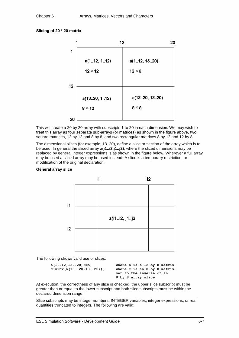
Chapter 6 Arrays, Matrices, Vectors and Characters
ESL Simulation Software - Development Guide 6-7
Slicing of 20 * 20 matrix
This will create a 20 by 20 array with subscripts 1 to 20 in each dimension. We may wish to treat this array as four separate sub-arrays (or matrices) as shown in the figure above, two square matrices, 12 by 12 and 8 by 8, and two rectangular matrices 8 by 12 and 12 by 8.
The dimensional slices (for example, 13..20), define a slice or section of the array which is to be used. In general the sliced array a(i1..i2,j1..j2), where the sliced dimensions may be replaced by general integer expressions is as shown in the figure below. Wherever a full array may be used a sliced array may be used instead. A slice is a temporary restriction, or modification of the original declaration.
General array slice
The following shows valid use of slices:
a(1..12,13..20):=b; where b is a 12 by 8 matrix
c:=inv(a(13..20,13..20)); where c is an 8 by 8 matrix
set to the inverse of an
8 by 8 array slice.
At execution, the correctness of any slice is checked, the upper slice subscript must be greater than or equal to the lower subscript and both slice subscripts must be within the declared dimension range.
Slice subscripts may be integer numbers, INTEGER variables, integer expressions, or real quantities truncated to integers. The following are valid:
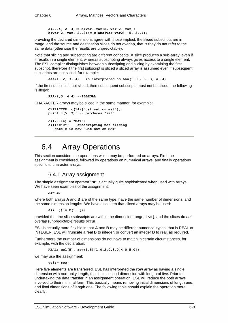
Chapter 6 Arrays, Matrices, Vectors and Characters
ESL Simulation Software - Development Guide 6-8
a(2..4, 2..4):= b(var..var+2, var-2..var);
b(var-2..var, 2..3):= c(abs(var-var2)..5, 3..4);
providing the declared dimensions agree with those implied, the sliced subscripts are in range, and the source and destination slices do not overlap, that is they do not refer to the same data (otherwise the results are unpredictable).
Note that slicing and subscripting are different concepts. A slice produces a sub-array, even if it results in a single element, whereas subscripting always gives access to a single element. The ESL compiler distinguishes between subscripting and slicing by examining the first subscript, therefore if the first subscript is sliced a sliced array is assumed even if subsequent subscripts are not sliced, for example:
AAA(1..2, 3, 4) is interpreted as AAA(1..2, 3..3, 4..4)
If the first subscript is not sliced, then subsequent subscripts must not be sliced; the following is illegal:
AAA(2,3..4,4) --ILLEGAL
CHARACTER arrays may be sliced in the same manner, for example:
CHARACTER: c(14)["cat sat on mat"];
print c(5..7); -- produces "sat"
c(12..14):= "MAT";
c(1):="C"; -- subscripting not slicing
-- Note c is now "Cat sat on MAT"
6.4 Array Operations This section considers the operations which may be performed on arrays. First the assignment is considered, followed by operations on numerical arrays, and finally operations specific to character arrays.
6.4.1 Array assignment
The simple assignment operator ":=" is actually quite sophisticated when used with arrays. We have seen examples of the assignment:
A:= B;
where both arrays A and B are of the same type, have the same number of dimensions, and the same dimension lengths. We have also seen that sliced arrays may be used:
A(i..j):= B(i..j);
provided that the slice subscripts are within the dimension range, i <= j, and the slices do not overlap (unpredictable results occur).
ESL is actually more flexible in that A and B may be different numerical types, that is REAL or INTEGER. ESL will truncate a real B to integer, or convert an integer B to real, as required.
Furthermore the number of dimensions do not have to match in certain circumstances, for example, with the declaration:
REAL: col(5), row(1,5)[1.0,2.0,3.0,4.0,5.0];
we may use the assignment:
col:= row;
Here five elements are transferred. ESL has interpreted the row array as having a single dimension with non-unity length, that is its second dimension with length of five. Prior to undertaking the data transfer in an assignment operation, ESL will reduce the both arrays involved to their minimal form. This basically means removing initial dimensions of length one, and final dimensions of length one. The following table should explain the operation more clearly:
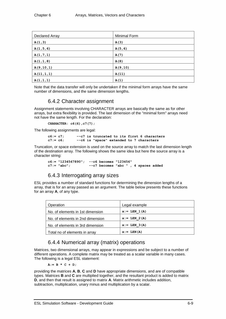
Chapter 6 Arrays, Matrices, Vectors and Characters
ESL Simulation Software - Development Guide 6-9
Declared Array Minimal Form
A(1,3) A(3)
A(1,5,6) A(5,6)
A(1,7,1) A(7)
A(1,1,8) A(8)
A(9,10,1) A(9,10)
A(11,1,1) A(11)
A(1,1,1) A(1)
Note that the data transfer will only be undertaken if the minimal form arrays have the same number of dimensions, and the same dimension lengths.
6.4.2 Character assignment
Assignment statements involving CHARACTER arrays are basically the same as for other arrays, but extra flexibility is provided. The last dimension of the "minimal form" arrays need not have the same length. For the declaration:
CHARACTER: c6(6),c7(7);
The following assignments are legal:
c6:= c7; --c7 is truncated to its first 6 characters
c7:= c6; --c6 is "space" extended to 7 characters
Truncation, or space extension is used on the source array to match the last dimension length of the destination array. The following shows the same idea but here the source array is a character string:
c6:= "1234567890"; --c6 becomes "123456"
c7:= "abc"; --c7 becomes "abc " , 4 spaces added
6.4.3 Interrogating array sizes
ESL provides a number of standard functions for determining the dimension lengths of a array, that is for an array passed as an argument. The table below presents these functions for an array A, of any type.
Operation Legal example
No. of elements in 1st dimension x:= LEN_1(A)
No. of elements in 2nd dimension x:= LEN_2(A)
No. of elements in 3rd dimension x:= LEN_3(A)
Total no of elements in array x:= LEN(A)
6.4.4 Numerical array (matrix) operations
Matrices, two dimensional arrays, may appear in expressions and be subject to a number of different operations. A complete matrix may be treated as a scalar variable in many cases. The following is a legal ESL statement:
A:= B * C + D;
providing the matrices A, B, C and D have appropriate dimensions, and are of compatible types. Matrices B and C are multiplied together, and the resultant product is added to matrix D, and then that result is assigned to matrix A. Matrix arithmetic includes addition, subtraction, multiplication, unary minus and multiplication by a scalar.
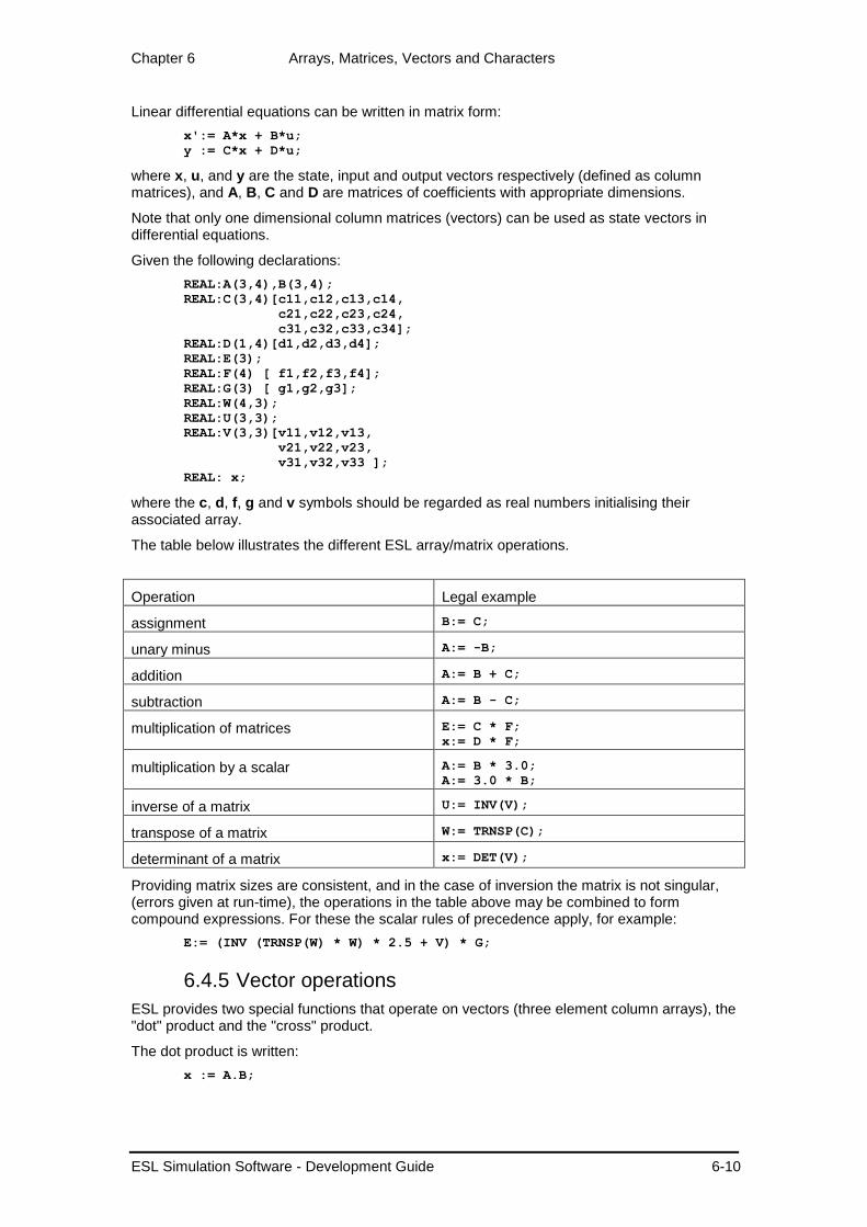
Chapter 6 Arrays, Matrices, Vectors and Characters
ESL Simulation Software - Development Guide 6-10
Linear differential equations can be written in matrix form:
x':= A*x + B*u;
y := C*x + D*u;
where x, u, and y are the state, input and output vectors respectively (defined as column matrices), and A, B, C and D are matrices of coefficients with appropriate dimensions.
Note that only one dimensional column matrices (vectors) can be used as state vectors in differential equations.
Given the following declarations:
REAL:A(3,4),B(3,4);
REAL:C(3,4)[c11,c12,c13,c14,
c21,c22,c23,c24,
c31,c32,c33,c34];
REAL:D(1,4)[d1,d2,d3,d4];
REAL:E(3);
REAL:F(4) [ f1,f2,f3,f4];
REAL:G(3) [ g1,g2,g3];
REAL:W(4,3);
REAL:U(3,3);
REAL:V(3,3)[v11,v12,v13,
v21,v22,v23,
v31,v32,v33 ];
REAL: x;
where the c, d, f, g and v symbols should be regarded as real numbers initialising their associated array.
The table below illustrates the different ESL array/matrix operations.
Operation Legal example
assignment B:= C;
unary minus A:= -B;
addition A:= B + C;
subtraction A:= B - C;
multiplication of matrices E:= C * F;
x:= D * F;
multiplication by a scalar A:= B * 3.0;
A:= 3.0 * B;
inverse of a matrix U:= INV(V);
transpose of a matrix W:= TRNSP(C);
determinant of a matrix x:= DET(V);
Providing matrix sizes are consistent, and in the case of inversion the matrix is not singular, (errors given at run-time), the operations in the table above may be combined to form compound expressions. For these the scalar rules of precedence apply, for example:
E:= (INV (TRNSP(W) * W) * 2.5 + V) * G;
6.4.5 Vector operations
ESL provides two special functions that operate on vectors (three element column arrays), the "dot" product and the "cross" product.
The dot product is written:
x := A.B;

Chapter 6 Arrays, Matrices, Vectors and Characters
ESL Simulation Software - Development Guide 6-11
and is a scalar quantity equal to the product of the magnitudes of the vectors multiplied by the cosine of the angle between them, as shown in the figure below.
Vector Dot Product
The cross product is written:
V := A^B;
Vector Cross Product
and is a vector of magnitude equal to the area of a parallelogram with A and B as adjacent sides, and in a direction perpendicular to the plane containing A and B, in a "right-hand sense", as shown in the figure above.
Provided that the matrices have appropriate dimensions, vector and matrix operations may be naturally combined, for example:
W' := INV(I)*(N-I*(W^N));
where I is a square matrix of size three and W and N are (3 element) vectors.
6.4.6 Array functions
ESL allows functions to be declared which return array values, for example:
PROCEDURE current(REAL:R(*,*),V(*)) RETURN REAL;
RETURN INV(R)*V;
END current;
For the matrix equation:
V = R * I
the procedure returns I given R and V, and could be used by a statement of the form:
I:=current(R,V);
where I, R and V have appropriate dimensions, and are REAL arrays.
The RETURN REAL in the procedure declaration only specifies that a REAL result is to returned (scalar or array), but the RETURN statement defines, computes and returns an array.

Chapter 6 Arrays, Matrices, Vectors and Characters
ESL Simulation Software - Development Guide 6-12
6.5 Character Array Operations In many respects CHARACTER arrays are treated in an identical manner to other array types. This section attempts to point out certain differences, and starts by introducing a different terminology which is used in certain cases.
A one dimensional array is termed a character string.
A two or three dimensional array is termed an array of characters.
A single CHARACTER variable is considered to be a one dimension character array of length one, and can be used in place of a character string except for subscripting and slicing.
6.5.1 Character array functions
The table below illustrates the special functions for use on character strings.
Operation Example
ASCII code (0 to 127 in decimal) of first character in character string argument
J:=IACHAR(C);
character value corresponding to the ASCII code (in decimal) of the integer argument
C:=ACHAR(J);
position of second string in the first string n:=SUB_STRING(C,C2);
no of characters in first dimension n:= LEN_1(C);
no of characters in second dimension n:= LEN_2(C);
no of characters in third dimension n:= LEN_3(C);
total no of characters in array n:= LEN(C)
The SUB_STRING function is identical in operation to the FORTRAN INDEX function, and will return zero if the sub-string is not found. The character variable may be replaced by literal characters as shown below:
character:string(16)/"This is a string"/;
character:subb(6)/"string"/;
....
print sub_string(string,subb);
print sub_string(string,"is");
print sub_string(string,"as");
The first print statement returns 11, the second 3 ("is" in "this") and the third a zero indicating not found. It is also possible to search for a character variable in a literal string, for example:
print sub_string("This is another string",subb);
will give the result 17.
The IACHAR function returns the ASCII character code of the character argument. For example, using the above string declaration, the following:
PRINT IACHAR(string);
PRINT IACHAR(string(1));
PRINT IACHAR(string(2));
will give 84 for "T" in the first two statements and 104 for "h" in the third. The function will differentiate between upper and lower case characters, and literal character strings may be used, as:

Chapter 6 Arrays, Matrices, Vectors and Characters
ESL Simulation Software - Development Guide 6-13
PRINT IACHAR("A");
PRINT IACHAR("a");
which will give 65 and 97 respectively.
The ACHAR function is the reverse of IACHAR, and returns a character corresponding to the ASCII code argument, for example:
i:=66;
j:=98;
PRINT ACHAR(i);
PRINT ACHAR(j);
which will print "B" and "b" respectively.
6.5.2 Character comparison
Literal strings and string variables may be used with the numerical relational operators in logical expressions, for example:
IF b = "abcdef" THEN
....
ELSE_IF b /= a THEN
....
END_IF;
When the lengths of the operand strings do not match, the shorter string is considered to be space extended.
The complete set of relational operators which may be applied to character strings is shown in the table below:
Relation Operation
s1 = s2 true if equal
s1 /= s2 true if not equal
s1 >= s2 true if greater than or equal
s1 > s2 true if greater than
s1<= s2 true if less than or equal
s1 < s2 true if less than or equal
For comparison purposes, the ASCII code of each character in the strings are compared, one by one starting at the left. As soon as an inequality is found the process is complete. The ASCII code reveals that "b" is greater than "a", "a" is greater than "A", "A" is greater than "2", and "2" is greater than "1".
6.5.3 Characters as subprogram arguments
Character variables, strings and character arrays may be used as arguments in calls to subprograms in the same way as other arrays, with the exception that the SUBMODEL does not allow CHARACTER output arguments.
Note that literal strings also may be actual arguments which correspond to formal arguments declared as a CHARACTER, character string or array.
6.5.4 Character function procedures
In the same way that function PROCEDUREs may return other arrays, they may also return CHARACTER arrays.

Chapter 7 Multivariable Transfer Functions
ESL Simulation Software - Development Guide 7-1
CHAPTER 7
7 Multivariable Transfer Functions This section describes the support ESL provides for "multivariable transfer functions". This allows a matrix of transfer functions with vector inputs and outputs to be set up.
Contents:
Introduction
Example 1 - Multivariable feedback control system
Example 2 - Coupled two-mass system
Limitations
7.1 Introduction A linear dynamic system having multiple inputs and multiple outputs may be described by means of a transfer function matrix, G(s). For example:
𝒀(𝑠) = 𝑮(𝑠)𝑼(𝑠)
where U(s) is an input vector, Y(s) is an output vector and G(s) is a matrix of transfer functions with appropriate dimensions.
In the ESL language, a linear multivariable system may be described by a TRANSFER_MATRIX statement, which must appear in the dynamic region of a program. The TRANSFER_MATRIX statement is an extension of the single variable TRANSFER statement and has the following form:
Y := TRANSFER_MATRIX ( transfer function matrix ) * expression;
The form of Y and expression are determined by the dimensions of the transfer function matrix. If the transfer function matrix has n rows and m columns, then Y must be declared as an n element real vector and expression must be an array expression which produces an m element real vector.
Note that in ESL an n x 1 matrix can be regarded as n element column vector, and a 1 x m matrix as a m element row vector.
If the transfer function matrix has a single row (1 x m), then Y may be a scalar variable or a 1 element vector. Similarly if the matrix has a single column (n x 1), then expression may be scalar or a 1 element vector.
The transfer function matrix must be factorised by finding the lowest common denominator of all its elements and expressing it in the following manner:
𝐺(𝑠) =1
𝑙𝑜𝑤𝑒𝑠𝑡 𝑐𝑜𝑚𝑚𝑜𝑛 𝑑𝑒𝑛𝑜𝑚𝑖𝑛𝑎𝑡𝑜𝑟[𝑚𝑎𝑡𝑟𝑖𝑥 𝑜𝑓 𝑛𝑢𝑚𝑒𝑟𝑎𝑡𝑜𝑟 𝑡𝑒𝑟𝑚𝑠]
For example:
𝐺(𝑠) =
[
(𝑠 + 1)
(𝑠 + 2)
𝑘
(𝑠 + 1)(𝑠 + 2)𝑘
(𝑠 + 1)(𝑠 + 2)
1
𝑠 ]
may be written as:
𝐺(𝑠) =1
𝑠(𝑠 + 1)(𝑠 + 2)[𝑠(𝑠 + 1)(𝑠 + 1) 𝑘𝑠
𝑘𝑠 (𝑠 + 1)(𝑠 + 2)]

Chapter 7 Multivariable Transfer Functions
ESL Simulation Software - Development Guide 7-2
A corresponding ESL statement is:
Y := TRANSFER_MATRIX( s(s + 1)(s + 2)
[ s(s + 1)(s + 1), k*s;
k*s, (s + 1)(s + 2) ]) * U;
where U and Y are two element input and output vectors (declared as REAL: U(2), Y(2); ).
The lowest common denominator appears first (not its reciprocal) followed by the numerator matrix enclosed by square brackets [ ]. Commas are used to separate matrix row elements, and semicolons to separate rows. The ESL compiler checks for consistency of the numerator matrix (same number of elements in each row), while dimensional compatibility of the input expression and output vector is checked at run time.
The syntax of the denominator and numerator terms is the same as for the TRANSFER statement with the addition that zeros (s, s**2 etc) may appear after the optional gain in the numerator terms. The following are acceptable numerators:
s 10*s 3.0*s**2 k*s(s + 1)(s + 2)
Use of the TRANSFER_MATRIX statement is illustrated in the following examples.
7.2 Example 1 - Multivariable feedback control system
The first example considers the multivariable feedback control system shown in the figure below.
Multivariable feedback control system
The control system forward path is given by:
𝐺(𝑠) =
[
1
(𝑠 + 1)−
1
𝑠2
𝑠
1
(𝑠 + 2)]
and the feedback path by:
𝐻(𝑠) = [1 00 1
]
The transfer function matrix is written in factorised form:
𝐺(𝑠) =1
𝑠(𝑠 + 1)(𝑠 + 2)[
𝑠(𝑠 + 2) −(𝑠 + 1)(𝑠 + 2)
𝑠(𝑠 + 1)(𝑠 + 2) 𝑠(𝑠 + 1)]
Since the transfer function matrix has dimensions 2 x 2, both the input and output of the TRANSFER_MATRIX statement must be arrays of dimensions 2 x 1.
The feedback path may be realised in this case by simply multiplying the control system output by a constant array. Had the feedback path been more complex, requiring a transfer

Chapter 7 Multivariable Transfer Functions
ESL Simulation Software - Development Guide 7-3
function description, a further TRANSFER_MATRIX statement could have been used in place of the multiplication.
An ESL program to simulate the response of the control system to a unit step applied to both inputs is given below. The program is provided in the ESL examples directory as mv_tfun1.esl. A post run plot generated from the prepare file, mv_tfun1.dsp using ISE, presents the results of the simulation.
-- Multivariable transfer function test program -
-- Control system
--
STUDY
MODEL multi_var_ctrl;
REAL: R(2)/2*1.0/, E(2), C(2), B(2),
H(2,2)[ 1.0, 0.0,
0.0, 1.1 ];
DYNAMIC
C := TRANSFER_MATRIX( s(s + 1)(s + 2)
[ s(s + 2), -(s + 1)(s + 2);
2(s + 1)(s + 2), s(s + 1) ] )*E;
E := R - B;
B := H*C;
STEP
PLOT "Multivariable control system", t, C(1), [C(2)],
0, tfin, 0, 2;
PREPARE " ", t, C;
END multi_var_ctrl;
--
multi_var_ctrl;
--
END_STUDY
Post-run plot from control system example

Chapter 7 Multivariable Transfer Functions
ESL Simulation Software - Development Guide 7-4
7.3 Example 2 - Coupled two-mass system
A second example considers a simple mechanical system comprising a double mass-spring-damper arrangement, as shown in the figure below. The arrangement is treated as a two-input, two-output system where the inputs are the forces applied to each of the two masses and the outputs are the linear positions of the two masses.
Coupled two-mass multivariable system
The system is described by the following equations:
𝑓1 − 𝐶1(𝑦1′ − 𝑦2
′ ) − 𝐾1(𝑦1 − 𝑦2) = 𝑀1𝑦1′′
𝑓2 + 𝐶1(𝑦1′ − 𝑦2
′ ) + 𝐾1(𝑦1 − 𝑦2) − 𝐶2𝑦2′ − 𝐾2𝑦2 = 𝑀2𝑦2
′′
which may be expressed in the Laplacian domain as:
[𝑀1𝑠
2 + 𝐶1𝑠 + 𝐾1 −𝐶1𝑠 − 𝐾1
−𝐶1𝑠 − 𝐾1 𝑀2𝑠2 + (𝐶1 + 𝐶2)𝑠 + (𝐾1 + 𝐾2)
] [𝑦1
𝑦2] = [
𝑓1𝑓2
]
By inverting the Laplacian matrix, the following is obtained:
[𝑦1
𝑦2] =
[ 𝑀2𝑠
2 + (𝐶1 + 𝐶2)𝑠 + (𝐾1 + 𝐾2)
𝛥(𝑠)
𝐶1𝑠 + 𝐾1
𝛥(𝑠)
𝐶1𝑠 + 𝐾1
𝛥(𝑠)
𝑀1𝑠2 + 𝐶1𝑠 + 𝐾1
𝛥(𝑠) ]
[𝑓1𝑓2
]
where
𝛥(𝑠) = 𝑀1𝑀2𝑠4 + (𝑀1𝐶1 + 𝑀1𝐶2 + 𝑀2𝐶1)𝑠
3 +
(𝑀1𝐾1 + 𝑀1𝐾2 + 𝑀2𝐾1 + 𝐶1𝐶2)𝑠2 + (𝐶1𝐾2 + 𝐶2𝐾1) + 𝐾1𝐾2
Thus the system may be described in terms of a transfer function matrix as:
𝒀 = 𝑮(𝑠)𝑭
where F is the input force vector, Y is the output position vector and G is the transfer function matrix given above.
The above model is expressed in terms of the ESL TRANSFER_MATRIX statement as:
Y := TRANSFER_MATRIX( (a0*s**4 + a1*s**3 + a2*s**2 + a3*s + a4)
[ (M2*s**2 + b1*s + b2), (C1*s + K1);
(C1*s + K1 (M1*s**2 + C1*s + K1) ] ) * F;
where a0, a1, .. , a4 and b1, b2 are pre-calculated Laplacian coefficients and both Y and F are declared as two element vectors.
The following is a listing of an ESL program to simulate the behaviour of the system to step input applied forces. The program, which appears in the ESL examples directory as

Chapter 7 Multivariable Transfer Functions
ESL Simulation Software - Development Guide 7-5
mv_tfun2.esl, generates the prepare file mv_tfun2.dsp. Graphical output generated by the Post Run Plot option of the ISE Display Manager is presented in the graph.
-- Multivariable transfer function test program -
-- Coupled two-mass system
--
STUDY
--
PACKAGE data;
---------------------------------------------------------
-- Mechanical system data:
--
-- m1, m2 masses;
-- c1, c2 damping coefficients;
-- k1, k2 spring coefficients;
-- f1, f2 constant applied forces.
---------------------------------------------------------
PARAMETER REAL: m1/0.1/, m2/1.0/,
c1/0.05/, c2/0.5/,
k1/2.0/, k2/1.0/,
f1/1.0/, f2/1.5/;
END data;
--
MODEL two_mass_m;
---------------------------------------------------------------
-- Transfer function matrix model.
-- Represents the system using a transfer function matrix
---------------------------------------------------------------
REAL: Y(2), F(2);
REAL: a0, a1, a2, a3, a4, b1, b2;
USE data;
INITIAL
a0 := m1*m2; a1 := m1*c1 + m1*c2 + m2*c1; a4 := k1*k2;
a2 := m1*k1 + m1*k2 + m2*k1 + c1*c2; a3 := c1*k2 + c2*k1;
b1 := c1 + c2; b2 := k1 + k2;
F(1) := f1;
F(2) := f2;
DYNAMIC
Y := TRANSFER_MATRIX(( a0*s**4 + a1*s**3 + a2*s**2 + a3*s
+ a4)[ (m2*s**2 + b1*s + b2), (c1*s + k1);
(c1*s + k1), (m1*s**2 + c1*s + k1) ] )*F;
STEP
PLOT "Coupled two-mass multivariable system",
t, Y(1), [Y(2)], 0, tfin, 0, 4;
PREPARE " ", t, Y;
END two_mass_m;
--
---------------------------------------------------------------
-- Experiment.
---------------------------------------------------------------
REAL: A(4,4), B(4,2), C(2,4), D(2,2);
USE data;
tfin := 20.0;
cint := 1.0;
nstep:= 10.0;
two_mass_m;
--
END_STUDY
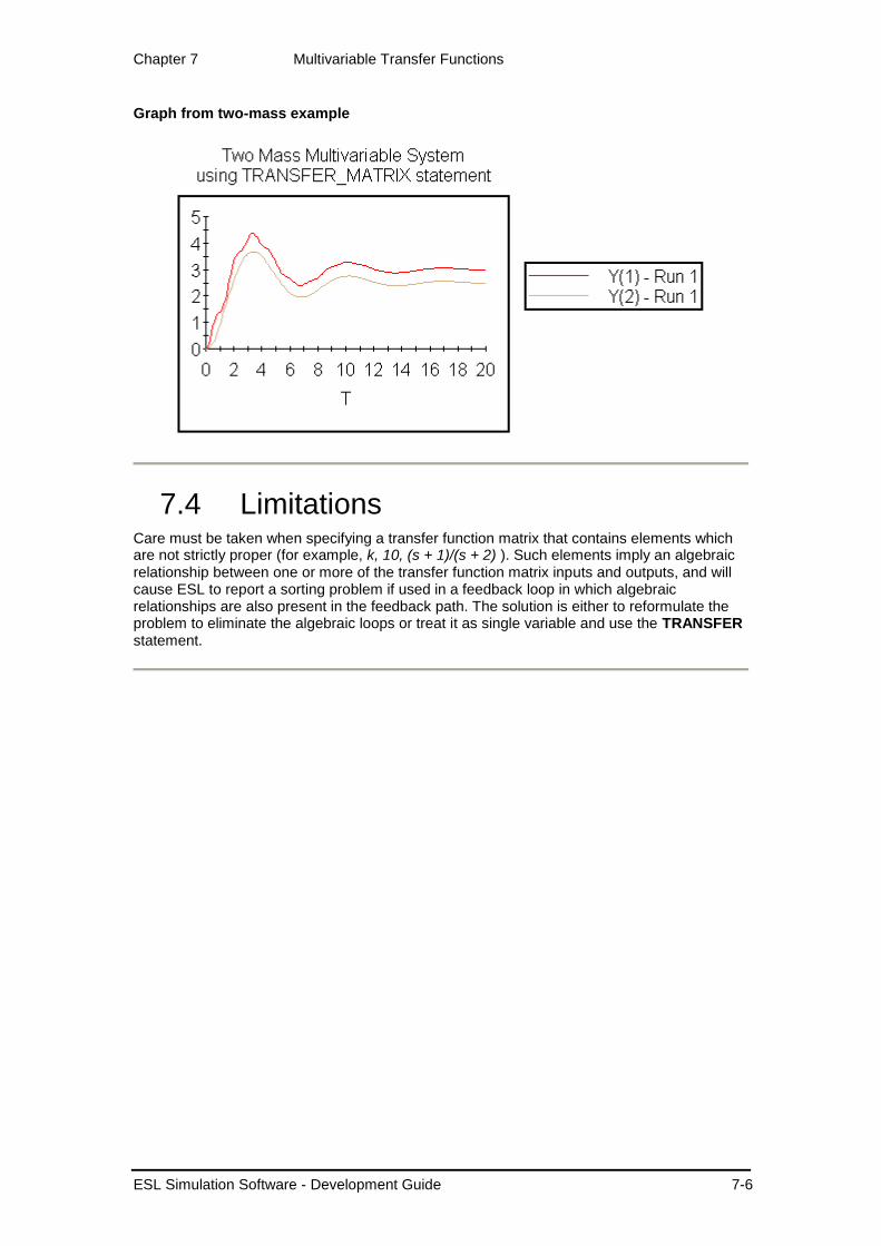
Chapter 7 Multivariable Transfer Functions
ESL Simulation Software - Development Guide 7-6
Graph from two-mass example
7.4 Limitations Care must be taken when specifying a transfer function matrix that contains elements which are not strictly proper (for example, k, 10, (s + 1)/(s + 2) ). Such elements imply an algebraic relationship between one or more of the transfer function matrix inputs and outputs, and will cause ESL to report a sorting problem if used in a feedback loop in which algebraic relationships are also present in the feedback path. The solution is either to reformulate the problem to eliminate the algebraic loops or treat it as single variable and use the TRANSFER statement.

Chapter 8 Input-Output and File Handling
ESL Simulation Software - Development Guide 8-1
CHAPTER 8
8 Input-Output and File Handling Although all ESL input and output can be managed from ISE, I/O support is provided through ESL program statements. This allows ESL programs to be run independently of ISE and customized for specific applications. When running an ESL program from ISE, ESL statement generated I/O can be used as an alternative to, or in addition to ISE specified output.
ESL provides comprehensive support for the input/output of text to the user terminal and files, and in addition it supports the output of graphical data. This section presents the text input/output statements PRINT, TABULATE and READ, and starts by describing how files are connected to an ESL program. Finally the graphical output support is presented.
Contents:
Connecting Files
File Deletion
Input/output Error Status
The PRINT Statement
The TABULATE Statement
The READ Statement
The PREPARE Statement
The PLOT Statement
The convertDisplayFile program
8.1 Connecting Files The ESL text input/output statements, PRINT, READ and TABULATE, may be optionally associated with a file rather than keyboard input or screen output. The link to a file is achieved by a "file-specifier" being connected to a file in a file connection statement. File-specifiers are declared in the same way as other variables, and the declaration comprises the keyword FILE: followed by one or more file-specifier names, for example:
FILE: infile, output, tempfile;
The file-specifier is connected to a text file by one of the following ESL statements:
OPEN
CREATE
REWRITE
Subsequent use of the file-specifier in READ, PRINT and TABULATE statements will then reference the connected file. The connection between specifier and file is broken by a CLOSE statement which allows the specifier to be reused. Any file-specifier that is not connected to a file will default to the terminal.
Note that file specifiers may be used as actual arguments of subprograms.
8.1.1 Opening, creating and rewriting files
Files may be connected to a file specifier in one of three ways:
Open - an existing file may be opened for reading.
Create - a new file may be created for writing (a file of the same name must not exist).
Chapter 8 Input-Output and File Handling
ESL Simulation Software - Development Guide 8-2
Rewrite - an existing file may be connected for writing in which case the original contents are over-written (lost), but if there is no existing file, this connection is the same as "create".
The ESL OPEN, CREATE and REWRITE statement perform the above file-specifier to file connection operations, and the CLOSE statement severs the connection. The OPEN statement connects a text file for reading, for example:
FILE: filespec;
....
OPEN filespec, "datafile.dat";
Here a file-specifier, filespec is connected to the existing file datafile.dat. If the file specifier is already connected to another file, that file will be disconnected, or closed, and a connection made to the new file. The file may be defined by a character expression or a character variable:
OPEN filespec, char_variable;
When the specified file cannot be opened, if, for example, the file does not exist, the user is prompted for an alternative file.
To allow the user program to handle such error conditions ESL allows all file connection statements to include a "status" option, for example:
OPEN filespec, "datafile.dat", IOSTAT=ERR;
In this case ERR is a user's integer variable which is set to indicate the status of the operation. If ERR is zero the operation was successfully completed, otherwise the value of ERR indicates the nature of the error. IOSTAT Errors shows possible error values for all input/output operations. This extension to the OPEN statement allows control to remain in the ESL program, and appropriate corrective action may be programmed. Note that with the status option there is no user interaction in the event of an error.
Once a file-specifier is linked to a file by the OPEN statement, the file's contents may be read into ESL by READ statements which use the file-specifier (see The READ Statement).
To open a file for output CREATE and REWRITE statements are provided. These statements are of the same format, and their operation only differs when the named file already exists. CREATE will create a new file if no file of the specified name already exists. If the file already exists the user will be prompted to indicate whether it may be overwritten, or to provide the name of an alternative file.
The REWRITE statement will over-write an existing file of the same name, otherwise it will create the required file. Examples of these statements are:
FILE: file1, file2;
....
CREATE file1, "datfile1.dat";
....
REWRITE file2, "datfile2.dat";
The status option also may be used here, in which case the user's program must handle the error conditions. Note there will be no user interaction in the event of a problem.
CREATE file1, "datfile1.dat",IOSTAT=ERR1;
....
REWRITE file2, "datfile2.dat",IOSTAT=ERR2;
PRINT and TABULATE statements may use file-specifiers, file1 and file2 to direct their text to the connected files.
ESL currently allows a maximum of 100 files to be connected at any one time.
8.1.2 Closing file connections
Following completion of file access, it is good practice to close the connection. The CLOSE statement disconnects the file from the file-specifier, which may then be reused, for example:

Chapter 8 Input-Output and File Handling
ESL Simulation Software - Development Guide 8-3
CLOSE file1;
This statement does not produce an error. All file connections are automatically closed at the end of the program.
8.2 File Deletion The DELETE statement physically deletes a file, which must not be connected to a file-specifier, for example:
DELETE "file1";
There are cases where deletion is not possible, for example, due to file protection mechanisms, or because the file is already connected to a file-specifier. Failure to delete will result in an error message, but the program continues. The status option may be used if the program wishes to check the success of the operation, for example:
DELETE "file1",IOSTAT=ERR;
See IOSTAT Errors for definition of status variable ERR.
8.3 Input/Output Error Status The following statements may include the error status option:
OPEN, CREATE, REWRITE, DELETE, READ, and READEL
The error status option must appear at the end of the statement, and has the general form:
... ,IOSTAT = err;
where err is a declared integer variable.
If the error specification is used, any errors encountered in the operation are returned as a code in err. If not used, the program will either interact with the user to resolve the problem, or in more serious cases abort. The status return codes are given in IOSTAT Errors.
IOSTAT Errors
Return value Status
0 Operation was performed without error
1 Eol was encountered when a data value was expected. A data value terminated by Eol does not cause the IOSTAT variable to be set to Eol
2 End-of-file was encountered
3 Error occurred converting input data to internal form- for example, illegal number format
4 Failure to open file
5 Create file failure - file already exists?
6 Failure to delete file
7 Failure to create file
8 Maximum file channels in use (>100)
9 Too many direct access files
10 File inaccessible - illegal name, already open?

Chapter 8 Input-Output and File Handling
ESL Simulation Software - Development Guide 8-4
8.4 The PRINT Statement The PRINT statement allows text and user variables to be output to the terminal screen or to a file. For example:
PRINT outfile, x*k, y, z;
PRINT outfile, "Results are:",x,y,z;
PRINT "Results are:", x,y,z;
The first two examples print data to a previously declared file-specifier which is connected to a file for output. If the file-specifier is unconnected output is directed to the terminal screen. The last example directs its output to the terminal. Note that expressions may be included in the output list.
If the output from a PRINT exceeds the width of one line (79 characters) further lines are output until the output list is exhausted. When more than one line is needed numerical and logical values are never split between lines, but always appear complete on one line. Character output, however, may be split between lines.
Printing arrays
The ESL PRINT statement for arrays, described in Arrays, Matrices, Vectors and Characters, clarifies understanding of the array initialisation process. The same examples are appropriate here. A full program is presented:
study
INTEGER: COL(5)[1,2,3,4,5], ROW(1,5)[1,2,3,4,5],
MAT_R(2,3) [11,12,13,
21,22,23],
MAT_C(2,3) /11,21,
12,22,
13,23/,
ARR(2,3,4) [111,112,113,114,
121,122,123,124,
131,132,133,134,
211,212,213,214,
221,222,223,224,
231,232,233,234];
PRINT "COL =",/,COL;
PRINT "ROW =",/,ROW;
PRINT "MAT_R=",/,MAT_R;
PRINT "MAT_C=",/,MAT_C;
PRINT "ARR =",/,ARR;
end_study
The results of this program follow:
COL =
1
2
3
4
5
ROW =
1 2 3 4 5
MAT_R=
11 12 13
21 22 23
MAT_C=
11 12 13
21 22 23
ARR =
111 112 113 114
121 122 123 124
131 132 133 134
211 212 213 214
221 222 223 224
231 232 233 234
Chapter 8 Input-Output and File Handling
ESL Simulation Software - Development Guide 8-5
The ESL PRINT statement outputs numerical arrays in row-major order, that is elements are processed in the order determined by changing the last subscript, in cyclic fashion, after each element is processed. The other subscripts are cycled in a similar fashion but at a lower frequency, the first subscript changing least frequently. The PRINT also "formats" the output by inserting "new-lines" each time the last subscript is changed to its lower dimension bound.
This rather complicated description simply means that arrays are presented in their natural mathematical order. That is:
A column vector is presented as a vertical column.
A row vector as a horizontal row.
A two-dimension matrix as a series of horizontal rows.
A three-dimension matrix, as a number (size of first dimension) of two-dimension matrices.
CHARACTER arrays are treated in a similar fashion, with one exception. That is a character column, one-dimension matrix, is presented as a horizontal row. The above example was modified to use CHARACTER arrays:
study
CHARACTER: COL(3)["col"], ROW(1,3)["row"],
MAT_R(2,3) ["cat",
"sat"],
MAT_C(2,3) /"cs","aa","tt"/,
ARR(2,3,4) ["cats",
"sat ",
"mats",
"CATS",
"SAT ",
"MATS"];
PRINT "**** COL <",COL,">";
PRINT "**** ROW <",ROW,">";
PRINT "**** MAT_R=",/,MAT_R;
PRINT "**** MAT_C=",/,MAT_C;
PRINT "**** ARR =",/,ARR;
end_study
This program gives the following results:
**** COL <col>
**** ROW <row>
**** MAT_R=
cat
sat
**** MAT_C=
cat
sat
**** ARR =
cats
sat
mats
CATS
SAT
MATS
Note that the column array/matrix has now been presented as a row. Also that, as far as printing is concerned, the row-major order is essential, see, for example, MAT_C the character array presented in column-major order.
Output format control (Data output formatting) applies to each element of an array.

Chapter 8 Input-Output and File Handling
ESL Simulation Software - Development Guide 8-6
8.4.1 Data output formatting
The default format used by the PRINT statement is:
REAL values: FORTRAN G13.5 (field width 13 characters, 5 significant digits, and room for exponent of four characters)
INTEGER values FORTRAN I9,4X (field width 9 characters, followed by 4 spaces)
LOGICAL values: 13 character field width (centred). The words TRUE or FALSE appear
To override the default format, the value to be output is followed by a colon, a whole number, and possibly a decimal part. That is. :m.n (for example, :12.5). This is interpreted as:
REAL values: if n /= 0 then (FORTRAN Fm.n) – field width m, with n decimal places; else_if n = 0 (that is, :m.0 or :m) then if m > 8 then FORTRAN Gm.(m-8) else_if m = 8 then FORTRAN G8.1 else_if m < 8 then FORTRAN G13.5 (the default format)
INTEGER values: field width m, right justified, FORTRAN Im
LOGICAL values: field width m, right justified
CHARACTER: are not influenced by format control
Note that a negative format specifier (for example, :-m.n or :-m) suppresses all spaces in output.
The maximum field width m is restricted to 24 characters.
The PRINT statement may also include line control characters:
/ forces a new line
-/ suspends a new line, next print will append;
To illustrate the general G format, consider format G12.4 which means a field of width 12 characters with 4 significant figures. This may be specified by x:12, and when x has the value -0.0003141592654 the output will be:
" -0.3142E-03"
Note that formatting real values with the "G" format requires a field width large enough for: possible negative sign; leading zero; decimal point; the specified number of significant figures; and four positions for a possible exponent.
The following example PRINT statements illustrate the use of formatting. Note that the ^ character is interpreted as a space:
REAL:x/202.4544/,y/22.55443/,z/3.1415926/;
INTEGER:a/3/,b/32/,c/321/;
LOGIC:logic_1/FALSE/;
PRINT x,y,z;
-- gives:
^^^202.45^^^^ -- 13 positions
^^^22.554^^^^ -- 13 positions
^^^3.1416^^^^ -- 13 positions
PRINT x:7.3,y:6.2,z:15.12;
-- gives:
202.454 -- 7 positions, 3 decimal places
^22.55 -- 6 positions, 2 decimal places
^3.141592600000 -- 15 positions,12 decimal places
PRINT a,b,c;
-- gives:
^^^^^^^^3^^^^ -- 9 positions, 4 trailing spaces
^^^^^^^32^^^^ -- as above

Chapter 8 Input-Output and File Handling
ESL Simulation Software - Development Guide 8-7
^^^^^^321^^^^ -- as above
PRINT a:4,b:6,c:8;
-- gives:
^^^3 -- 4 position field
^^^^32 -- 6 position field
^^^^^321 -- 8 position field
PRINT logic_1;
-- gives:
^^^^FALSE^^^^ -- centred in 13 position field
PRINT logic_1:3;
-- gives:
FAL -- truncated to formatted field
The "/" is used as a PRINT element to force a new line, whereas a "-/" is normally used at the end of the PRINT to suppress the normal end-of-print new line. For example:
PRINT "This is one line",/,"and this is the next",-/;
PRINT " but this continues on the second line";
gives the output:
This is one line
and this is the next but this continues on the second line
8.5 The TABULATE Statement A TABULATE statement is designed for use during a simulation run to output results in text form from the COMMUNICATION or STEP region. In these cases a heading is output at the start of each simulation run, and data values are output at each communication or step point. This creates a table arranged in columns with appropriate variable names at the top of each column.
The format of the TABULATE statement is illustrated by the following examples:
TABULATE tabfile, a,b,c;
Output will be directed to the file to which file-specifier tabfile is connected, or to the terminal if the file-specifier is not connected. The output contains the headings, a, b and c, and then the tabular data.
TABULATE "file",t,x,y;
TABULATE " ",t,x,y;
In the first case the data will be output to file.tab, which will be automatically connected (REWRITE mode), and overwrite any existing file of the same name. If the file name is specified as " ", than the file used will be the name of the program with a .tab extension. The default extension .tab is used unless the file is specified with an explicit extension. Whenever the program is restarted, including a "restart" from the INTERACT facility (ESL Run Control), the tabulate file will be overwritten.
TABULATE a,b,c*2, array1;
This example directs output to the terminal, and shows the use of a scalar expression, and an array variable. Arrays are output in row-major order.
The data is output using default formats. Note that the RESERVED variable DIS_ST may be used, with an IF statement, to control the frequency of output in the STEP region.
A file created by a TABULATE statement during a simulation run, which only contains numerical or logical data, may be converted to PREPARE format through an ISE file menu option or the convertDisplayFile program, in order to present results graphically as well as in Tabular form.
A TABULATE statement may be used outside the dynamic loop of the simulation in which case both the headings and the values are output each time the statement is executed.

Chapter 8 Input-Output and File Handling
ESL Simulation Software - Development Guide 8-8
The maximum number of variables permitted in a TABULATE statement is actually determined by the character length of each of the TABULATE elements, and is approximately 100.
8.6 The READ Statement The READ statement may accept text input from the keyboard, or from a file connected to a file-specifier, for example:
READ filespec, I, V, R;
Here I, V and R are read from the file connected to the file-specifier filespec. If the file-specifier is omitted (or is not connected to a file) the READ statement will take its input from the keyboard, for example:
READ I, V, R;
The READ list may include user variables of any type, and also array variables and slices are allowed.
In these examples the data to be read should be presented in "free format" style.
8.6.1 Free format input
Unless the READ statement specifies explicit format control (see Data input formatting) the input data may be presented in free format. Free-format input allows all data items to be presented on a single line, or the data items may be spread over several lines. An individual data item must not be split by a line boundary, and each new READ statement requires its data to start on a new line.
Each data item may be preceded by spaces, and must be terminated with a space, comma, equal sign ("="), or eol (end-of-line). In particular:
INTEGER values may be preceded by an optional plus or minus, immediately followed by the integer value. No embedded spaces are allowed. Any decimal point will cause rejection of the value.
REAL values may be preceded by an optional plus or minus. They may be entered as integers, or may start, or end, with a decimal point, and may also include an exponent (for example, -4.12e-5).
CHARACTER strings must be presented within string quotes (" or %), or as un-quoted strings which do not contain embedded spaces, commas or equals (=) signs. The character string may be extended, or truncated, to match the number of characters required to fill the variable specified in the READ. The character data must not be split over a line boundary, and it does not undergo case conversion (for example, lower to upper case).
LOGICAL values are treated as character strings, which must match one of the following:
True False
true false
tru fals
tr fal
t fa
yes f
ye no
y n
1 0
During READ processing, the input is read, a line at a time, into an input buffer. An attempt is then made to set each variable in the READ statement list to the corresponding data value

Chapter 8 Input-Output and File Handling
ESL Simulation Software - Development Guide 8-9
from input buffer. Leading spaces are ignored, and if a valid delimiter (comma, equal sign or eol) is encountered when a data value is expected then:
REALs are given the value 0.0.
INTEGERs are given the value 0.
LOGICALs are set to false.
CHARACTER strings are space filled.
The following example illustrates free format input:
REAL: x; INTEGER:i; LOGICAL: L; CHARACTER ch(4);
....
READ x,i,L,ch;
Any of the following sets of input data would satisfy the READ:
3.1415926 12345 true abcd
0.31415926e1 12345 T "abcd"
.31415926e1,12345,1,"abcd"
-3.14,,,"a"
The first three examples are equivalent, setting x:=3.1415926, i:=12345, L:= true, and ch:="abcd". The last example of input data would set x:=-3.14, i:=0, L:=false, and ch:="a ".
Reading arrays
Array variables, or slices, may appear in a READ statement, and ESL interprets this as though each element of the array is presented separately, in row-major order (Arrays, Matrices, Vectors and Characters). CHARACTER arrays, however, are a little more complex.
CHARACTER array data is expected in row-major order, but the last dimension is treated as a single character string, for example:
CHARACTER: c4(4), c24(2,4);
....
read c4;
read c24;
One character string would satisfy the first READ, for example, the following responses would result in the setting c4 as shown:
Response: ABCD sets c4 := "ABCD";
A sets c4 := "A ";
While the second READ requires two character strings, for example:
Response: abcde 123
Sets c24(1..1, 1..4) := "abcd", and c24(2..2, 1..4) := "123 ".
Format control (see below) used with an array implies all that elements of the array are subject to the format specification.
8.6.2 Keyboard input
During keyboard input ESL will interact with the user in an attempt to correct input data which would otherwise result in an error. Consider the example:
READ I, V, R;
ESL will generate a default prompt of "I, V, R:" to remind the user what input is required. If a more explicit prompt is required this may be provided as a character string following the keyword READ, for example:
READ "Input V (volts), I (amps) and R (ohms): ", I,V,R;
or as a character variable (string), or expression, enclosed in ( ) brackets, for example:
READ (char_variable), I, V, R;

Chapter 8 Input-Output and File Handling
ESL Simulation Software - Development Guide 8-10
The ( ) brackets are necessary to distinguish the character variable as a prompt, and not as an item to be read.
To satisfy this READ the user may type the first value followed by Return/Enter, and if that input was valid for the type of "I" then the user would be prompted:
Enter value for item 2:
In response, the user may enter data values for the next list variable (V), or indeed for all remaining data (that is, for V and R) to satisfy the READ. If any data value is illegal the process will be restarted from the input list variable corresponding to the illegal data, and the user will be prompted to give data for that variable and all remaining variables.
Format specifiers (see below) may be used to override the default free format input conventions, although such specifiers are not normally useful during keyboard reading. There is one exception, however - when reading character data, it may be desirable to override the default situation of allowing either upper or lower case characters. The format specifier ":0.1" will convert all characters to upper case.
A keyboard break (Ctrl-Break or Ctrl-C) during input will cause control to be passed to the INTERACT service. Note if the operating system screen, rather than the ESL controlled screen, is being used it is normally necessary to press Return/Enter immediately following the break key.
8.6.3 The READEL statement
The READEL (read next element) statement provides a means of reading data one element at a time. After a READ is complete the remaining input line characters which have not been processed may be read with one or more READEL statements. It operates in the same way as a READ but takes its input data from the characters remaining in the buffer (those which have not yet been processed). The format of the READEL statement is the same as READ but it may not have a file-specifier.
The following examples, which are functionally equivalent, illustrate the relationships between READ and READEL (note the ":" is for format control described in Data input formatting).
READ infile, a, b:6, c:10;
is equivalent to:
READ infile;
READEL a, b:6, c:10;
and also to:
READ infile,a;
READEL b:6;
READEL c:10;
The READEL may be used if the format of the data depends on the first data element read. For example, the following section of code prompts the user to respond with the number of data items to read in, and then to provide the specified number of data items:
REAL:num;
INTEGER: x;
....
READ "Input number of items, followed by values: ", num;
FOR i:=1..num LOOP
READEL x, IOSTAT=err;
IF err /= 0 THEN
PRINT "data format error";
STOP;
END_IF;
-- process x
....
END LOOP;
If the user responds to the prompt with:
Input number of items, followed by values: 4 1.0 2.0 3.0 4.0

Chapter 8 Input-Output and File Handling
ESL Simulation Software - Development Guide 8-11
The data values will be processed as:
READ num = 4
READEL x = 1.0 1st pass of loop, i = 1;
READEL x = 2.0 2nd pass, i = 2;
READEL x = 3.0 3rd pass, i = 3;
READEL x = 4.0 4th pass, i = 4
Additional examples are given in READ examples.
8.6.4 Data input formatting
Formatting of inputs is provided by following the variable name with a colon and a whole number with an optional decimal part, that is, :m.n (for example, :12.1) or :m (for example, :8).
For the whole number part m:
An m of zero (that is, 0.0 or 0.1) is the default situation and free format input applies.
A positive m specifies a fixed-field of m characters, for example, var:4.0, means the data for var is in the next field of 4 characters.
A negative m (that is, :-1, :-1.0 or :-1.1) means free format, but only that line is to be analyzed; the reading of a subsequent line is not permitted to satisfy the current list item.
The decimal part n applies to character string input only, and indicates conversion to upper case that is:
m.0 means no conversion of case (the default);
m.1 conversion to upper-case.
For fixed-field format, leading and trailing spaces are ignored for numerical and logical values, and a field which comprises entirely of spaces is considered to give a data value of zero, or false for logical items. Furthermore if a valid number, which is properly delimited, is encountered before the end of the field, the remainder of the field is ignored.
For character string variables read in fixed format, the m input characters are assigned to the string variable with truncation or space extension if the length of the variable string is different from n. Note that spaces, commas, equals and quote characters are permitted in these fixed format strings.
If an eol (end-of-line) is encountered during fixed-format reading when a new data field is expected an error condition exists, and if present the IOSTAT variable will be set to indicate the eol. If the IOSTAT variable is not present the program continues without reporting an error. Any remaining input list items will be given their default values, that is, zero for numbers, space for characters, and false for logical.
If the start of a fixed-format field exists, but there are less than n characters before an eol is encountered, the input field is considered to be extended by spaces until it is n characters long. This case is not considered an error, and the IOSTAT variable is not set to indicate eol.
Format specifiers to allow fixed format file records to be input, are illustrated by:
READ infile, i:2, j:3, x:6, c1(1..3):2, c2(1..3):4.1, ch:1.0;
where i and j are integers; x is real; c1 and c2 are one-dimension character arrays, or strings, and ch is a character variable.
If the file input line is:
123456.7890abcdefgh
the format specifiers partition the line into fields which are illustrated by using a "|" character to indicate the field boundaries:
|12|345|6.7890|ab|cdef|g|hijklm
This causes the following assignments:
Chapter 8 Input-Output and File Handling
ESL Simulation Software - Development Guide 8-12
i = 12
j = 345
x = 6.7890
c1(1..3) = "ab " -- field is space extended to fit c1
c2(1..3) = "CDE" -- field is truncated to fit c2,
-- conversion to upper case with :4.1
ch = "g"
Note that the remainder of the input line, "hijklm", is not used.
A second example shows how a READ with a mixture of format specified input, and free format input is processed. Consider the statement:
READ infile, i, j:3, x:6, c1(1..3):2.0, c2(1..3), c3:1.1;
and the input line:
61 123 4.56 abcde,x
using the "|" character to separate the fields gives:
| 61 |123| 4.56 | a|bcde,|x|
- :3 :6 :2.0 - :1.1 -- formats
Note that in the cases of free format the delimiting character (a space) is associated with the field it is delimiting, and the next character processed is the character after the delimiter.
This input line causes the following assignments:
i = 61
j = 123
x = 4.56
c1(1..3) = " a " -- field restricted 2 characters and then
-- space extended to fit c1(1..3)
c2(1..3) = "bcd" -- field is truncated to fit c2.
c3 = "X" -- conversion to upper case.
8.6.5 READ examples
The following two examples illustrate the flexibility of the READ and READEL statements, and emphasise the detailed operation of the statements.
The following code counts the number of characters (trailing spaces ignored), and lines in a file. It illustrates how a normal text file may be read character by character.
character: ch; FILE: infile;
INTEGER: err,count,lines;
....
OPEN infile, ...
....
count:= 0; -- no of characters
lines:= 0; -- no of lines
loop
READ infile, IOSTAT=err;
terminate err /= 0; -- End-of-file
lines:= lines + 1;
loop
READEL ch:1, IOSTAT=err;
terminate err /= 0; -- End-of-Line
-- Count the characters
count:= count + 1;
end_loop;
end_loop;
Another example where the READEL statement is useful is when optional items may be appended to an input line, for example, a section of a data file may be:
1.0 1.2
2.0 4.4 VOLT= 20.0
3.0 9.6
4.0 16.8 voltage=10

Chapter 8 Input-Output and File Handling
ESL Simulation Software - Development Guide 8-13
5.0 26.0
...
A section of code to read the data follows:
REAL: x, y, Volt;
CHARACTER: ch;
INTEGER: err;
FILE: infile;
....
OPEN infile, ...
....
loop
read infile,x,y,IOSTAT=err;
terminate err /= 0; -- end-of-file? Exit loop.
-- Read rest of line and convert string to upper case, (:-1.1)
readel ch:-1.1, IOSTAT=err;
-- If no string found ch will be set to " "
-- IOSTAT is unnecessary but can indicate string found, that
-- is, err=0
-- or err /= 0 if not found.
if ch = "V" then
-- A string starting with "V" or "v" found, note the whole
-- string is processed and the "=" acts as a delimiter.
-- A real value should now follow.
readel Volt,IOSTAT=err;
if err /= 0 then STOP; end_if; -- An error!
....
end_if;
end_loop;
input_output
8.7 The PREPARE Statement The PREPARE statement is designed to be used in the COMMUNICATION or STEP region to record the results of a simulation for subsequent graphic analysis by the Post Run Plot option of the ISE Display Manager (see the Integrated Simulation Environment (ISE)) or with the convertDisplayFile program. It creates a non-text file (REWRITE mode) over-writing any existing file of the same name. The output file is specified by a literal string, a blank string (interpreted as file name of program with .dsp extension), or a character variable. Note that the output cannot be directed to the terminal, and a file-specifier may not be used. Typical PREPARE statements are:
PREPARE "example",t,x,y*z,array1,array2(2..4,2);
PREPARE " ",t,x,y,z;
PREPARE t,y/2,det(array1);
If no file extension is given, ESL will assume ".dsp". Note that any previous copy of the prepare file will be overwritten by a new simulation run - this also applies when the program is restarted from the INTERACT facility, ESL Run Control. The PREPARE list may include numerical or logical variables or expressions, and also arrays and array expressions. Note that a logical true is interpreted as 1.0, and false as zero.
Multiple PREPARE statements are permitted in a subprogram, and the contents of PREPARE files may be converted into TABULATE file format by the ISE file menu option.
It is possible to extend the PREPARE statement by including a title, subtitle and annotations for each of the variables. The general format is shown:
PREPARE "file", "Title", "Subtitle",t,"(variable name)",
x,"(variable name)",array1(1..2,2);
These optional descriptions are stored in the prepare file and are accessible when the file is processed by ISE.

Chapter 8 Input-Output and File Handling
ESL Simulation Software - Development Guide 8-14
The PREPARE statement is intended to be used like the TABULATE statement, and the two are often complimentary with the TABULATE output being in text form, while the PREPARE output is in a form suitable for graphical display. PREPARE statements appearing outside the COMMUNICATION or STEP regions create a single data set (equivalent to one run).
Up to 100 variables can be included in a PREPARE statement.
8.8 The PLOT Statement A PLOT statement produces graphical output during the course of a simulation run, and is normally placed in the STEP or COMMUNICATION region. The first execution draws the axis and presents the headings, and subsequent executions plot the data points, joined by straight lines. Real, integer and logical types may be plotted (logical types are treated as 1 for true, or 0). Multiple runs of the simulation may be displayed (the line from the last data point of the previous run to the first point of the new run is suppressed).
If a PLOT statement is placed outside the STEP or COMMUNICATION regions it produces a plot with symbols only, that is the data points are not joined by lines.
Multiple PLOT statements may be specified in a program - each will create its own plotting window.
The general format for a PLOT statement is quite specific since it is necessary to define not only the variables, but the scale of the axis:
PLOT "Optional title", x/10, y*1000 [abs(y2),y3],
tmin, tmax, y_min, y_max;
where:
x is the x-axis independent variable
y is the y-axis dependent variable
y2, y3 are additional y-axis variables
tmin is the start of the x-axis scale
tmax is the end of the x-axis scale
y_min is the start of the y-axis scale
y_max is the end of the y-axis scale
Several variables may be inserted between the optional "[ ]" brackets, after the first y-axis variable. The variables may be scalars or scalar expressions of type real, integer or logical. Note that axis limits may be general scalar expressions, and often the x-axis is defined as:
.... , 0, tfin, ...
8.9 The CLEAR_SCREEN statement The CLEAR_SCREEN statement closes all open plot windows and prohibits further output from currently active plot statements. Any new plot statements encountered after a clear screen will open new plot windows.
8.10 The convertDisplayFile program The convertDisplayFile program plots or converts an ESL display file (i.e. either a prepare (.dsp) or tabulate (.tab) file) to another format.
Usage: convertDisplayFile [option] ESL-display-file [output-file]
where option:
[none] - convert ESL-display-file a prepare or tabulate file to the
opposite
-csv - convert the ESL-display-file to a comma separated values file
-tsv - convert the ESL-display-file to a tab separated values file
-plot - plot the ESL-display-file (any output-file is ignored)

Chapter 8 Input-Output and File Handling
ESL Simulation Software - Development Guide 8-15
To plot a display file use the option '-plot' without an output file. This is usually done for a prepare file but will also work for a tabulate file.
To change the format from a prepare file to a tabulate file, or vice versa, use no option.
To convert a display file into a textual format suitable for importing in to other programs, such as spreadsheet applications (e.g. Microsoft Excel or OpenOffice.org Calc) the options '-csv' and '-tsv' may used to create 'comma separated values' or 'comma separated values' output files.

Chapter 9 ESL Segments
ESL Simulation Software - Development Guide 9-1
CHAPTER 9
9 ESL Segments This section describes the ESL segment concept, and shows how this may be used for distributed and embedded simulation.
Contents:
Introduction
Emulated Segment Operation
Distributed Simulation Execution
Embedded Segments
Generation of Interface Modules for ESL Embedded Segments
9.1 Introduction There are two types of segment in ESL - an embedded segment and a parallel segment. An embedded segment is a form of ESL model that can be embedded in a C++ or FORTRAN program. Parallel segments allow an ESL program to be partitioned into modules that can be run concurrently.
ESL provides the means to:
Emulate a multi-processor environment on a single computer, and execute parallel segments within a single program (Emulated Segment Operation).
Execute the simulation on multi-processors or a distributed network of processors, with each segment being "remotely" executed by a separate process (Distributed Simulation Execution).
Embed the segment in a C++ or FORTRAN program, which calls the segment simulation step-by-step (Embedded Segments).
Distributed Simulation

Chapter 9 ESL Segments
ESL Simulation Software - Development Guide 9-2
Embedded Simulation
The first part of this section introduces ESL segments and illustrates their use in an emulated environment. Then consideration is given to how the segments may be executed using separate processes, and the final section shows how segments may be embedded into a C++ or FORTRAN main program.
9.2 Emulated Segment Operation Emulated segments allow the simulation performance of a true multi-processor machine to be predicted, and they offer many advantages to the simulation engineer even in a conventional processor environment. The separate processors are synchronised to exchange data with other processors at fixed communication points, that is after fixed intervals of simulated time.
9.2.1 The multi-processor concept
The ESL program segment structure provides the means of partitioning a system specification into a multi-processor environment. A complete dynamic system may be specified as being partitioned into a model, which is regarded as the master segment, and one or more segments. The model and each segment describe a subset of the complete system, and the ESL program code for the model, and each segment, is considered to reside and be executed on separate processors.
The underlying concept is that the simulation of the model partition is proceeding on one processor at the same time as the simulation of each segment partition on other processors. When the model and all segment simulations have completed a communication interval, data is exchanged between the processors. Only after this data exchange, or synchronisation point, is the simulation resumed in each segment and the model.
All communication is channelled through the master segment, the model, which has the ability to communicate with all other segments. In the communication region the model receives output data from all segments, and then after execution of the communication region the model passes input data to each segment in turn and this causes the simulation to continue in that segment.
With several segments it is possible to define different communication intervals for data communication between the model and particular segments. The model works with the basic communication interval, but it may communicate with a segment that has a communication interval that is a multiple of the basic communication interval. This allows lower frequency segments to have longer communication intervals, and this technique is described in more detail later.

Chapter 9 ESL Segments
ESL Simulation Software - Development Guide 9-3
The concurrent execution of segment simulation is emulated by ESL, but the result is the identical to that which would be obtained in a true multi-processor situation as described later in this section. The Segment Emulation figure below shows the execution sequence. Note how the segment simulation advances prior to that of the model, but the results are only passed to the model during the model's communication region. This last point is illustrated more clearly in the Segment Timing figure below.
9.2.2 Emulated segment
Segment timing
Note that the segment call may be conditional, that is the subject of an IF statement. Any number of segments may be specified and run simultaneously. The call to the segment in the communication region basically has the task of receiving the output argument values from the
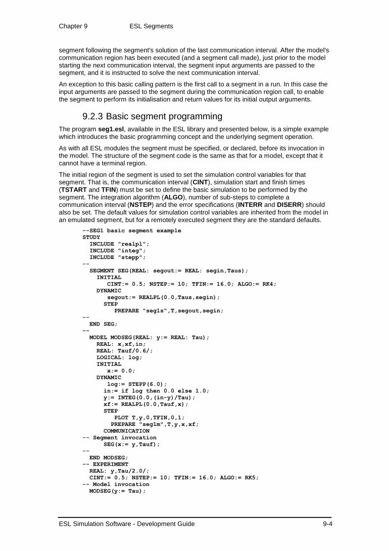
Chapter 9 ESL Segments
ESL Simulation Software - Development Guide 9-4
segment following the segment's solution of the last communication interval. After the model's communication region has been executed (and a segment call made), just prior to the model starting the next communication interval, the segment input arguments are passed to the segment, and it is instructed to solve the next communication interval.
An exception to this basic calling pattern is the first call to a segment in a run. In this case the input arguments are passed to the segment during the communication region call, to enable the segment to perform its initialisation and return values for its initial output arguments.
9.2.3 Basic segment programming
The program seg1.esl, available in the ESL library and presented below, is a simple example which introduces the basic programming concept and the underlying segment operation.
As with all ESL modules the segment must be specified, or declared, before its invocation in the model. The structure of the segment code is the same as that for a model, except that it cannot have a terminal region.
The initial region of the segment is used to set the simulation control variables for that segment. That is, the communication interval (CINT), simulation start and finish times (TSTART and TFIN) must be set to define the basic simulation to be performed by the segment. The integration algorithm (ALGO), number of sub-steps to complete a communication interval (NSTEP) and the error specifications (INTERR and DISERR) should also be set. The default values for simulation control variables are inherited from the model in an emulated segment, but for a remotely executed segment they are the standard defaults.
--SEG1 basic segment example
STUDY
INCLUDE "realpl";
INCLUDE "integ";
INCLUDE "stepp";
--
SEGMENT SEG(REAL: segout:= REAL: segin,Taus);
INITIAL
CINT:= 0.5; NSTEP:= 10; TFIN:= 16.0; ALGO:= RK4;
DYNAMIC
segout:= REALPL(0.0,Taus,segin);
STEP
PREPARE "seg1s",T,segout,segin;
--
END SEG;
--
MODEL MODSEG(REAL: y:= REAL: Tau);
REAL: x,xf,in;
REAL: Tauf/0.6/;
LOGICAL: log;
INITIAL
x:= 0.0;
DYNAMIC
log:= STEPP(6.0);
in:= if log then 0.0 else 1.0;
y:= INTEG(0.0,(in-y)/Tau);
xf:= REALPL(0.0,Tauf,x);
STEP
PLOT T,y,0,TFIN,0,1;
PREPARE "seg1m",T,y,x,xf;
COMMUNICATION
-- Segment invocation
SEG(x:= y,Tauf);
--
END MODSEG;
-- EXPERIMENT
REAL: y,Tau/2.0/;
CINT:= 0.5; NSTEP:= 10; TFIN:= 16.0; ALGO:= RK5;
-- Model invocation
MODSEG(y:= Tau);

Chapter 9 ESL Segments
ESL Simulation Software - Development Guide 9-5
--
END_STUDY
Segmentation example
The simulation control (reserved) variables for each segment are unique, and the model and other segments may select different values. ESL maintains a separate set of simulation control variables for each segment. Care must be taken, however, to ensure that the segment's communication interval is an integer multiple of that set in the model, and that it is consistent with the frequency at which the segment is invoked from the model.
In contrast, the simulation control variables for the model either may be set in the experiment or the model's initial region. The model or experiment has the task of setting the basic communication interval (CINT). This defines the highest frequency at which inter-segment communication can take place. The final time (TFIN) should be set by the model, and the simulation run may also be stopped prematurely by TERMINATE statements in any segment.
The segment invocation must always be in the model communication region and the calling statement has the same form as a model invocation in the experiment. Each segment may be called once only during a pass of the communication region. By the use of conditional IF statements a segment may be invoked every nth communication interval pass rather than each pass. In this case the segment must have a communication interval set to (n * CINT).
Basic segment example
Examination of the example reveals that the model solves a subsystem which produces the result (y) of an exponential response, first increasing from zero and then, at time 6.0, decaying back to zero. Note the use of INCLUDE statements to access the library submodels REALPL (real-pole), INTEG (integrator) and STEPP (step input at T = 6.0).
The value of y is passed to the segment SEG as an input argument. The output from the segment invocation is x, which is also used in the model code of the dynamic region. Therefore x must be initialised prior to entering the dynamic region for the first time. This initialisation is only effective during model initialisation and is correctly updated by the segment invocation before the simulation commences.
The segment takes y as its input SEGIN and subjects this to filtering by a real-pole, or lag, to produce the segment output (SEGOUT).
The model receives the segment output in its variable x which it filters by a real-pole to produce xf.
Results from the Model shows the results from the model's point of view. The output from the segment (x) is updated at each communication interval and therefore has the "staircase" characteristic shown in the graph.
Results from the Segment shows the results from the segment's point of view. The input to the segment SEGIN is updated at each communication interval, and it also has the "staircase" characteristic.
Understanding the segment results
This example clearly shows the fundamental characteristics of parallel processing. That is, the discretisation of data communicated between processors, and the lag, or delay, inherent in this process. In effect, the example passes the value of y to a segment which simply returns it. A comparison of y and xf shows the effect of communication of data to a segment, and then the communication of the segment response back to the model.
Inter segment communication errors
During inter-segment communication there is both a phase and amplitude error which is dependent on the communication interval, and data is available only at discrete intervals in time which results in a stepped or staircase waveform. If proper account is taken of this fundamental operation, segmentation can be used to produce very efficient results even on a single processor segment emulation.

Chapter 9 ESL Segments
ESL Simulation Software - Development Guide 9-6
Results from the model
Results from the segment
In many simulations, the errors introduced by inter-segment communications are small and do not materially change the results of the simulation. In other cases, however, the errors have a critical influence on the simulation and action must be taken to reduce or eliminate the errors. In order for a user to determine the problems associated with a particular system it is advisable to be able to compare segmented results with known correct solutions. In other words, it is prudent to first simulate the basic system without using segments to produce a set of "correct" results. These results provide an invaluable source of data to validate the segmented results.
A system is often segmented to produce a fast simulation time in a production environment, where the basic simulation is to be repeated many times. In order to gain this speed advantage with multi-processors, or even with an emulation, without sacrificing accuracy it is necessary to develop the segmented simulation with great care. It is surprisingly easy to produce a segmented simulation which is both slower and less accurate than its unsegmented equivalent.

Chapter 9 ESL Segments
ESL Simulation Software - Development Guide 9-7
Choice of communication interval
The objective is to select the largest communication interval (CINT), to minimise the overhead caused by the number of inter-segment communication, which still gives satisfactory results.
The communication interval, however, determines the communication bandwidth, which together with the frequency (or rate of change) of data to be communicated determines the error introduced. The selection of the communication interval should be based on the highest frequency to be communicated between segments. If Wh is the highest frequency communicated between segments, and Tp the corresponding period, then a communication interval of:
CINT = Tp/36 -- where Tp = 2*pi/Wh
will introduce a phase-lag of about 10 degrees as the data is transferred between segments. This selection of communication interval, possibly used in connection with appropriate correction (see below), should prove adequate in most cases.
It should be noted that higher frequencies of communicated data require smaller communication intervals, and hence increased communication overhead. Furthermore the smaller communication interval may force integration in one or more segments to use inefficiently small step-lengths. This can cause a segmented solution to run slower than the unsegmented program. Therefore the manner in which a system is partitioned may be critical.
Partitioning a system into segments
The system should be partitioned into segments keeping in mind the following guidelines:
Partition the system at natural boundaries - this often helps to satisfy the following points. If the system includes a digital control or computer control section, this is often an excellent choice for a segment. Function generation is also a good candidate.
Minimise the interconnection between segments.
Minimise the frequency of data communicated between segments.
The best candidates for segmentation are often those parts of a system which have a different range of frequencies compared with the rest of the system. In the case of a low frequency segment, which also communicates with the remainder of the system at a low frequency, a much larger integration step-length may be used in the segment. On the other hand, a high frequency segment, which communicates with the remainder of the system at low frequency, gives a similar advantage. In this case the remainder of the system may use the larger integration step-length.
Produce an equitable balance in computer power required to simulate each segment, for example, a similar number of differential equations. The final simulation execution time will depend on the time taken to execute the most complex segment.
9.3 Distributed Simulation Execution This section describes how the simple ESL example, seg1.esl shown above, may be executed on a network of distributed processors. Differences in configuration and execution for Linux and MS Windows platforms are described. A sensible starting point in the generation of a distributed computer simulation is to validate the simulation with a single process using ESL's segment emulation facilities. This process was described in the first part of the section.
Preparing remote segment
The next step is to separate the segment code which is to be executed as a separate process to the experiment and model. For example, create the file remseg.esl (from original seg1.esl):

Chapter 9 ESL Segments
ESL Simulation Software - Development Guide 9-8
REMOTE
INCLUDE "realpl";
--
SEGMENT SEG(REAL: segout:= REAL: segin,Taus);
INITIAL
CINT:= 0.5; NSTEP:= 10; TFIN:= 16.0; ALGO:= RK4;
DYNAMIC
segout:= REALPL(0.0,Taus,segin);
STEP
PREPARE "seg1s",T,segout,segin;
--
END SEG;
The syntax for a remote segment specifies that there should be no model, no experiment and one and only one SEGMENT. Note the program starts with the keyword REMOTE, and there is no END_STUDY. Submodels, or procedures, which are needed by the segment should be declared prior to the segment in the normal ESL fashion. In this case one submodel "REALPL", from the library is required.
This file should be moved to the processor where it is to be remotely executed. Note ESL must be established on that processor and the environmental variables ESLPROG and ESLLIB should be set. Then the one of the following commands may be issued to build the executable:
esl -cccl remseg - to build via C++ translation
esl -cfl remseg - to build via FORTRAN translation
The remote program remseg is now ready.
Main simulation or client
Now create the ESL (model) program which will invoke the remote segment (remseg). First copy seg1.esl to new file main_mod.esl, and then modify the segment declaration by adding the word EXTERNAL before the semi-colon that is:
SEGMENT SEG(REAL: segout:= REAL: segin,Taus) EXTERNAL;
This causes the ESL compiler to ignore the body of the segment, which may be removed if desired. In addition, the code normally generated to emulate the segment is replaced by code to invoke and execute the segment remotely. The added code maintains appropriate synchronised communications with the remote segment.
An executable program is generated by:
esl -cccl main_mod - for a C++ build
esl -cfl main_mod - for a FORTRAN build
We now have a client (main_mod) and a server (remseg) executable programs.
Note: The model (master segment) and all remote segments must be built with the same precision (single or double). We recommend using either C++ or FORTRAN builds for all segments.
Configuration considerations
In order to run the newly created segment on a remote machine, the user must have certain capabilities and have configured certain files:
The user must be able to launch and run a process on the remote machine using one of the available protocols (rsh, ssh and esl - see Launching remote segment).
Where ESL has not been installed and setup on the remote machine (which does not apply for the esl protocol), the script esl_attach (esl_attach.bat for MS Windows) must be copied to the remote machine and made accessible to the user (e.g. by putting it on the PATH). This script is provided in the ESL executable directory (environment variable ESLPROG).
The remote segment program and files must be accessible on the remote machine, either by creating the program directly on the remote machine or creating it on the same kind of machine and copying the file to the remote machine.
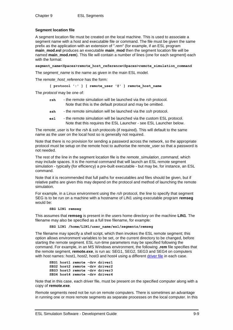
Chapter 9 ESL Segments
ESL Simulation Software - Development Guide 9-9
Segment location file
A segment location file must be created on the local machine. This is used to associate a segment name with a host and executable file or command. The file must be given the same prefix as the application with an extension of ".rem" (for example, if an ESL program main_mod.esl produces an executable main_mod then the segment location file will be named main_mod.rem). This file will contain a number of lines (one for each segment) each with the format:
segment_name<Spaces>remote_host_reference<Spaces>remote_simulation_command
The segment_name is the name as given in the main ESL model.
The remote_host_reference has the form:
[ protocol ':' ] [ remote_user '@' ] remote_host_name
The protocol may be one of:
rsh - the remote simulation will be launched via the rsh protocol.
Note that this is the default protocol and may be omitted.
ssh - the remote simulation will be launched via the ssh protocol.
esl - the remote simulation will be launched via the custom ESL protocol.
Note that this requires the ESL Launcher - see ESL Launcher below.
The remote_user is for the rsh & ssh protocols (if required). This will default to the same name as the user on the local host so is generally not required.
Note that there is no provision for sending a password across the network, so the appropriate protocol must be setup on the remote host to authorise the remote_user so that a password is not needed.
The rest of the line in the segment location file is the remote_simulation_command, which may include spaces. It is the normal command that will launch an ESL remote segment simulation - typically (for efficiency) a pre-built executable - but may be, for instance, an ESL command.
Note that it is recommended that full paths for executables and files should be given, but if relative paths are given this may depend on the protocol and method of launching the remote simulation.
For example, in a Linux environment using the rsh protocol, the line to specify that segment SEG is to be run on a machine with a hostname of LIN1 using executable program remseg would be:
SEG LIN1 remseg
This assumes that remseg is present in the users home directory on the machine LIN1. The filename may also be specified as a full tree filename, for example:
SEG LIN1 /home/LIN1/user_name/esl/segments/remseg
The filename may specify a shell script, which then invokes the ESL remote segment; this option allows environment variables to be set, or the current directory to be changed, before starting the remote segment. ESL run-time parameters may be specified following the command. For example, in an MS Windows environment, the following .rem file specifies that the remote segment, remote.exe, is run as: SEG1, SEG2, SEG3 and SEG4 on computers with host names: host1, host2, host3 and host4 using a different driver file in each case.
SEG1 host1 remote -drv driver1
SEG2 host2 remote -drv driver2
SEG3 host3 remote -drv driver3
SEG4 host4 remote -drv driver4
Note that in this case, each driver file, must be present on the specified computer along with a copy of remote.exe.
Remote segments need not be run on remote computers. There is sometimes an advantage in running one or more remote segments as separate processes on the local computer. In this

Chapter 9 ESL Segments
ESL Simulation Software - Development Guide 9-10
case the host name should be that of the local computer. Alternatively, the local computer will be assumed if a "-" is substituted for the host name. If, in the previous example, SEG1 and SEG2 were to run on the local computer, the .rem file would be:
SEG1 - remote -drv driver1
SEG2 - remote -drv driver2
SEG3 host3 remote -drv driver3
SEG4 host4 remote -drv driver4
Executing distributed simulation
Start the main ESL program (main_mod). This will attempt to start processes for any external segments which have been declared in the ESL program (that is, SEG). This is achieved by reading the main_mod.rem file for information on the required location of each segment and starting each remote process using the rsh command. Each remote process will connect back to the main model and a message confirming the successful establishment of the communications link will be displayed. The ESL model and segments will now run; on completion the model will instruct the segments to exit. If either program terminates abnormally (for example, CTRL-C is typed) then the other program will report an error and exit.
The results obtained should be identical to those for the emulated segment.
The Remote Segment Call and Remote Segment Execution figures below show the execution sequence for a remote segment call.
Remote segment call

Chapter 9 ESL Segments
ESL Simulation Software - Development Guide 9-11
Remote segment execution
Launching remote segment
ESL supports three protocols for launching a remote segment simulation program on a remote host. The original (default), rsh and the more secure ssh protocols which allow a process to started on a remote host in the context of a user of the remote host.
Note that the rsh command was supported on versions of Windows below Vista but required the installation of a special rshd server. This protocol is no longer always supported on Linux platforms (depending on the distro).
Note that the ssh command is well supported on Linux but is not readily available (in a suitable command format) on Windows.
The installation and configuration of the rsh & ssh protocols, which are standards, is not covered in this document.
The third protocol supported is a custom esl protocol that requires the ESL Launcher service program.
ESL Launcher
The ESL Launcher service is available in ESL-Pro, which must be fully authorised (i.e. not authorised by being in the evaluation period) on both the local host and the remote host. It is provided by the program esl_launcher (for the remote host) and there is a utility program ping_esl_launcher which may be used on the local host to check for connectivity.
This custom secure protocol runs over a direct socket TCP/IP protocol, using default port 3377, which may be changed by an environment variable ESL_LAUNCHER_PORT (which has to be the same on both the local and remote hosts).
Note that the remote host firewall may have to have been set to permit access to the port for the ESL Launcher program.
The esl_launcher program
This program is run on the command line and is used in the following manner:
Usage: esl_launcher ( [-h] | [-q] [-d] )
Waits for a command to launch an ESL remote segment.
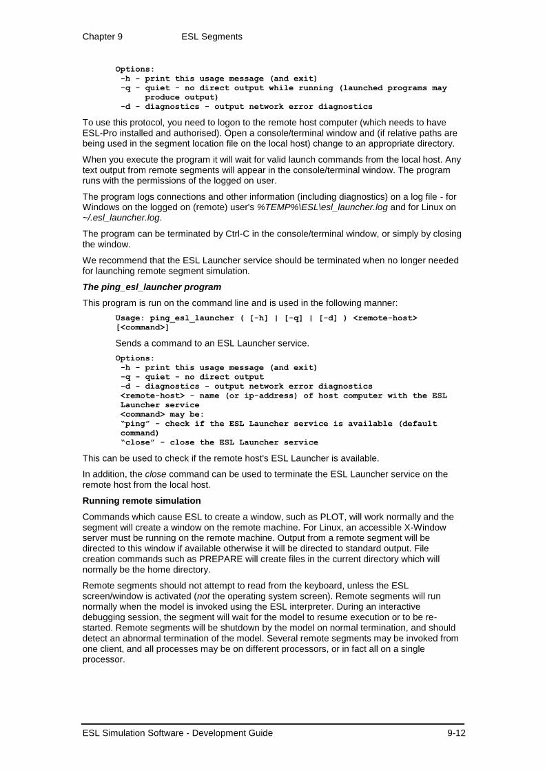
Chapter 9 ESL Segments
ESL Simulation Software - Development Guide 9-12
Options:
-h - print this usage message (and exit)
-q - quiet - no direct output while running (launched programs may
produce output)
-d - diagnostics - output network error diagnostics
To use this protocol, you need to logon to the remote host computer (which needs to have ESL-Pro installed and authorised). Open a console/terminal window and (if relative paths are being used in the segment location file on the local host) change to an appropriate directory.
When you execute the program it will wait for valid launch commands from the local host. Any text output from remote segments will appear in the console/terminal window. The program runs with the permissions of the logged on user.
The program logs connections and other information (including diagnostics) on a log file - for Windows on the logged on (remote) user's %TEMP%\ESL\esl_launcher.log and for Linux on ~/.esl_launcher.log.
The program can be terminated by Ctrl-C in the console/terminal window, or simply by closing the window.
We recommend that the ESL Launcher service should be terminated when no longer needed for launching remote segment simulation.
The ping_esl_launcher program
This program is run on the command line and is used in the following manner:
Usage: ping_esl_launcher ( [-h] | [-q] | [-d] ) <remote-host>
[<command>]
Sends a command to an ESL Launcher service.
Options:
-h - print this usage message (and exit)
-q - quiet - no direct output
-d - diagnostics - output network error diagnostics
<remote-host> - name (or ip-address) of host computer with the ESL
Launcher service
<command> may be:
“ping” - check if the ESL Launcher service is available (default
command)
“close” - close the ESL Launcher service
This can be used to check if the remote host's ESL Launcher is available.
In addition, the close command can be used to terminate the ESL Launcher service on the remote host from the local host.
Running remote simulation
Commands which cause ESL to create a window, such as PLOT, will work normally and the segment will create a window on the remote machine. For Linux, an accessible X-Window server must be running on the remote machine. Output from a remote segment will be directed to this window if available otherwise it will be directed to standard output. File creation commands such as PREPARE will create files in the current directory which will normally be the home directory.
Remote segments should not attempt to read from the keyboard, unless the ESL screen/window is activated (not the operating system screen). Remote segments will run normally when the model is invoked using the ESL interpreter. During an interactive debugging session, the segment will wait for the model to resume execution or to be re-started. Remote segments will be shutdown by the model on normal termination, and should detect an abnormal termination of the model. Several remote segments may be invoked from one client, and all processes may be on different processors, or in fact all on a single processor.

Chapter 9 ESL Segments
ESL Simulation Software - Development Guide 9-13
Conclusions
Only examples that lend themselves to simulation by the segment approach will benefit from distributed processing. The speed of calculation is determined by the process that requires the longest execution time to simulate a single frame. Therefore in cases where different speed processors are involved, it is important to put the slowest process on the fastest processor. The best results are obtained for simulations that require considerable computation per frame, and the work is evenly divided between the processes.
Note that distributed processing is not only used to speed a simulation, but also to introduce: real-time synchronisation; human or hardware in the loop; special animation or display processes; non ESL software which conforms to the ESL segment protocol, that is, FORTRAN, C or C++.
Note that REMOTE segments may be called from the communication region of either a model or an embedded segment.
ESL provides the interface (segment protocol) to exploit distributed multi-process simulation.
9.4 Embedded Segments Facilities are provided for embedding an ESL simulation within a C++ or FORTRAN main program, and invoking and controlling the simulation from the C++ or FORTRAN code. In addition, ESL programs may invoke non-ESL routines written in FORTRAN, C or C++, by specifying EXTERNAL routines (External Procedures).
An ESL segment and its supporting submodels may be executed in a step-by-step style, that is, the simulation may be advanced a frame (CINT) at a time, for example:
Simulation input is specified.
The simulation advanced by one frame (CINT).
The simulation results returned, the C++/FORTRAN program may now do other operations before advancing the simulation over the next frame.
The main program - ESL data communication is achieved by means of C++ class member variables or FORTRAN common variables.
In the case of C++ embedded programs when running MS Windows, ESL provides a facility for generating interface modules such as dynamic link libraries (DLL's), ActiveX COM objects and .NET assemblies, which can be used directly in Microsoft Visual C++ or C# (.NET) projects.
9.4.1 Embedded simulation using FORTRAN
To illustrate the ESL embedded simulation, let us consider a simple example. First the simulation should be expressed as a segment within an ESL EMBEDDED program, for example, in a file embseg.esl:
embedded
package esl_io;
real: out,inp,outo/0.0/,tau/0.6/;
end esl_io;
--
segment embed;
use esl_io;
real: y;
initial
y:=outo;
dynamic
y':=-(y-inp)/tau;
communication
out:=y;
tabulate " ",t,inp,out;

Chapter 9 ESL Segments
ESL Simulation Software - Development Guide 9-14
prepare " ",t,inp,out;
end embed;
This is a very simple system that subjects the input inp to a first-order lag to produce the output out. The initial value of output is outo. Note the information to be communicated to the segment is specified in the package esl_io, which contains the input, output, initial condition and also the time-constant of the filter tau. An embedded program starts with the keyword EMBEDDED, it must have one, and only one, segment, and the segment must not have arguments (data is communicated by packages). The program must not contain a model, an experiment, or an END_STUDY statement. Note the output out should only be set in the COMMUNICATION, not the DYNAMIC, region.
In this example we have used the ESL TABULATE and PREPARE statements to give post-mortem information.
Before reaching this stage it is advisable to have tested the segment code with a model emulating the FORTRAN program. The study embemu.esl was used for this task, that is:
study
package esl_io;
real: out,inp,outo/0.0/,tau/0.6/;
end esl_io;
--
segment embed;
use esl_io;
real: y;
initial
y:=outo;
dynamic
y':=-(y-inp)/tau;
communication
out:=y;
tabulate " ",t,inp,out;
prepare " ",t,inp,out;
end embed;
model mod;
real: x,y;
use esl_io;
constant real: w/1.0/;
initial
y:=outo;
dynamic
x:= sin(w*t);
y':=-(y-x)/tau;
communication
inp:=x;
embed;
prepare "nonemb",t,x,y,out;
plot t,y,[out],0,tfin,-1,1;
end mod;
-- experiment
cint:=0.2;
algo:=2;
mod;
end_study
This study actually duplicates the required simulation in the model, and passes the same inputs to the segment for the segmented solution. The duplication was performed to ensure that the segmentation approach did not introduce unacceptable errors (see the first part of this section).
With the segment tested we may now call it from a FORTRAN program with a high degree of confidence. First create FORTRAN subroutines corresponding to embseg.esl by using the ESL compiler and Translator, that is, embseg.f (or embseg.f).
The test program embprg.f (or embprg.f for MS Windows systems) illustrates how the main program controls the simulation.

Chapter 9 ESL Segments
ESL Simulation Software - Development Guide 9-15
* embprg.f/for
*
PROGRAM MAIN
INCLUDE 'eslcxx.dat'
* Reserved common extracted from Translated Embedded program
* embseg.esl.
* COMMON must be identical to that generated by current ESL
Translator.
REAL T,TSTART,TFIN,CINT,DISERR,INTERR,OP_STP
INTEGER ALGO,NSTEP,GE_EUL,WK$RNT,WK$SIM,IEX_CM,WK$PAR,DIS_ST,
*WK$MOD,WK$Y0,WK$YMX,WK$COM,MD$SYM
COMMON/RESERVED/T,TSTART,TFIN,CINT,DISERR,INTERR,OP_STP,ALGO,NSTEP
*,GE_EUL,WK$RNT,WK$SIM,IEX_CM,WK$PAR,DIS_ST,WK$MOD,WK$Y0,WK$YMX,
*WK$COM,MD$SYM,IF$1(31)
SAVE /RESERVED/
* ESL_IO common extracted from Translated Embedded program embseg.esl
REAL OUT,INP,OUTO,TAU
COMMON/ESL_IO/OUT,INP,OUTO,TAU
SAVE /ESL_IO/
REAL W
INTEGER STATUS
EXTERNAL EXP$MN,FINX
*
* Initialise embedded software
CALL EXP$MN(EXSTRT,STATUS)
* After initialisation of embedded esl, the RESERVED and EMBED common
* blocks may be freely changed, NOT before.
* We shall change: finish time, CINT and ALGO
* Mark above store allocated in setup
CALL MARKX
TFIN=8.0
CINT=0.2
ALGO=2
PRINT *,' '
PRINT *,'1st run with sin(t) input, CINT=',CINT,' and TAU=',TAU
PRINT *,' '
W=1.0
* Set input for simulation initialisation
INP=SIN(W*T)
* Now initialise the simulation
CALL EXP$MN(EXINIT,STATUS)
* Start simulation loop
10 CONTINUE
* Set input for simulation
IN=SIN(W*T)
* Output results
print *,'Time,inp,out',T,INP,OUT
* Have we done
IF(T.LE.14.0)THEN
* Advance simulation by one frame
CALL EXP$MN(EXSIM,STATUS)
IF(STATUS.EQ.CXOK)THEN
* Simulation completed task
GOTO 10
ELSEIF(STATUS.EQ.CXTERM)THEN
* Simulation terminated normally, but ignore
GOTO 10
ELSE
* Something went wrong
STOP
ENDIF

Chapter 9 ESL Segments
ESL Simulation Software - Development Guide 9-16
ENDIF
*
* Lets do another run
* We shall change: finish time, and time constant.
TFIN=12.0
TAU=2.4
PRINT *,' '
PRINT *,'Second run with step input TFIN=',TFIN,' and TAU=',TAU
PRINT *,' '
* Set input for simulation initialisation
INP=0
* Change initial start value
OUTO=0.1
* Now initialise the simulation
CALL EXP$MN(EXINIT,STATUS)
* Start simulation loop
20 CONTINUE
* Set input for simulation
INP=1.0
* Output results
print *,'Time,inp,out',T,INP,OUT
* Have we done
IF(STATUS.EQ.CXOK)THEN
* Advance simulation by one frame
CALL EXP$MN(EXSIM,STATUS)
GOTO 20
ELSEIF(STATUS.EQ.CXTERM)THEN
* Simulation terminated normally
PRINT *,'Run terminated by embedded simulation'
ELSE
* Something went wrong
PRINT *, 'Run aborted by embedded simulation'
ENDIF
* Close simulation
CALL EXP$MN(EXFIN,STATUS)
END
The FORTRAN program performs two complete simulations; in the first the modelled system is subject to a sine wave input, while in the second to a step input. Let us consider various aspects of this program.
Program notes
The include file eslcxx.dat is distributed with ESL in the ESL executable directory (environment variable ESLPROG). It defines enumeration constants or keys which define simulation functions, and status return values. In this example it is assumed it has been copied to the directory containing the example code.
The COMMON blocks, RESERVED and ESL_IO, have been extracted from embseg.f (or embseg.f), and provide the means for communicating data between the FORTRAN main program and the simulation. Note that it is important to copy the COMMON blocks code from the generated FORTRAN code (rather than typing it in by hand) to avoid introducing errors.
The simulation run-time support routines must be initialised prior to any other simulation call by:
CALL EXP$MN(EXSTRT,STATUS)
This call should be made once only, and it also has the function of initialising reserved variables to their default values, and package variables where initial values are specified, for example, OUTO and TAU.
Prior to a simulation the simulation COMMON variables must be set appropriately. In particular the input to the segment must be set (INP), and any initial conditions (OUTO). Note

Chapter 9 ESL Segments
ESL Simulation Software - Development Guide 9-17
that the segment initial region may be used to set CINT, ALGO etc, in which case the segment code will take precedence over COMMON data set at this point.
The simulation must be initialised (the segment initial region, dynamic and communication regions are executed) prior to starting the simulation run. This is achieved by the FORTRAN statement:
CALL EXP$MN(EXINIT,STATUS)
which returns output (OUT) resulting from the initialisation.
At this point the simulation loop is constructed:
This starts with setting COMMON variables defining simulation inputs ( IN).
Output is now consistent, that is the output (OUT) corresponds to the simulation time (T), and the input (INP) is the value of simulation input at the same simulation time. This is therefore a good point to output any results.
The simulation is advanced by one frame (CINT) by: CALL EXP$MN(EXSIM,STATUS) this integrates the solution over a communication interval and finally executes the segment communication region. Time (T) has been advanced and the simulation output (OUT) now corresponds to time T.
The status variable (STATUS) is set: CXOK no problems; CXTERM simulation has been completed normally, that is, T has advanced to TFIN. This may be safely ignored, but if an explicit TERMINATE statement was used in the ESL code then the simulation must not be continued. CXSTOP means a severe error, possibly integration failure has occurred (this cannot occur with the explicit integration routines). More serious problems cause an error message and the program is stopped by ESL.
After advancing the simulation, the FORTRAN program may perform other tasks using the result from the simulation. It is also the point where the input to the next frame may be computed from other processes, or even obtained from hardware or a user interface.
The example shows two styles of simulation loop.
A further simulation may be performed by repeating the above steps, except the EXSTRT call. The example shows such a second simulation run. Note that ESL treats this second run correctly, for example, prepare files will contain two separate sets of results.
Terminate the simulation runs by:
CALL EXP$MN(EXFIN,STATUS)
which closes any open ESL files.
ESL/FORTRAN conflicts
Problems may arise due to conflicts between the FORTRAN main program and the ESL generated FORTRAN; the following indicates how to avoid possible problems.
Subroutine and common names
The names of ESL generated subroutines, functions and common blocks are based on the user's ESL code and care should be taken to ensure they do not conflict with names in the calling FORTRAN program. The ESL run-time support library has many routines and several common blocks. These names are always six or less characters and end with the letter X. ESL also generates names containing a $ (or other system dependent special FORTRAN identifier characters). Avoiding names for subroutines and common blocks which may clash with ESL names will prevent problems.
Input/Output
An ESL program may open a number of FORTRAN file channels for PREPARE, TABULATE and other user specified file operations. ESL can possibly open FORTRAN file channels 7 to 27, and it is advised that these channels are not used by the FORTRAN calling program.

Chapter 9 ESL Segments
ESL Simulation Software - Development Guide 9-18
Embedded ESL for graphics
A FORTRAN program which needs graphics capability may use the ESL plot and prepare facilities, by using a special embedded segment. The segment could have a empty dynamic region (just the keyword DYNAMIC), and specify PLOT or PREPARE in the communication region.
Building embedded program
The following sequence of commands builds the embedded simulation study:
esl -c embseg
esl -tf embseg
esl -f embseg
The file embseg.f is produced from the above; the FORTRAN program is compiled with:
esl -f embprg
and the embedded ESL and the FORTRAN are linked by:
esl -fl embprg embseg
this produces the executable program embprg, which may be executed by:
esl -x embprg
or by simply:
embprg (or ./embprg)
The result of running embprg is to produce terminal tabulation from the FORTRAN program (embprg.f or .f), and a prepare file embseg.dsp, and tabulate file embseg.tab from the ESL segment (embseg.esl).
All programs illustrated in this section are provided in the ESL library directory.
9.4.2 Embedded simulation using C++
Using the same ESL example as was used to illustrate FORTRAN embedding, the following esl commands:
esl -c embseg
esl -tcc embseg
generate the C++ source file embseg.cpp, which corresponds to the embedded simulation.
C++ Code Using Embedded ESL
The C++ main program in file embprg_cpp.cpp, in the ESL examples directory illustrates how the embedded simulation is called from the C++ main program. That is:
// embprg_cpp.cpp/cpp
#include <math.h>
#include <stdio.h>
#include "rt_sup.h"
class s__simulation;
// Class Esl_io obtained from embseg.cpp/cpp
class Esl_io__c
{
public:
real Out,Inp,Outo,Tau;
void set__up(void);
public:
void setSimulation(s__simulation* s);
s__simulation* s_;
};
// Class Embed obtained from embseg.cpp/cpp
class Embed: public s__model

Chapter 9 ESL Segments
ESL Simulation Software - Development Guide 9-19
{
private:
real Y,Y_;
int W__1,W__2,W__3,W__4;
public:
Embed(void);
void e__1(void);
void e__2(void);
void e__3(void);
public:
void setSimulation(s__simulation* s);
s__simulation* s_;
};
// Simulation context obtained from embseg.cpp/cpp
class s__simulation : public s__simulation_c
{
public:
s__simulation();
//Experiment
void Exp_mn(int W__1, int &W__2);
// External classes
Esl_io__c Esl_io;
Embed x__1;
public:
s__simulation* s_;
};
int main(int argc, char *argv[])
{
real w = 1.0;
int status;
s__simulation* s = new s__simulation(); // Simulation context.
// Initialise embedded software
s->Exp_mn(EXSTRT, status);
// We shall change: finish time, CINT and ALGO
s->Reserved.Tfin = 8.0;
s->Reserved.Cint = 0.2;
s->Reserved.Algo = 2;
printf(
"\nFirst run with sin(t) input, CINT=%f and TAU=%f\n\n",
s->Reserved.Cint, s->Esl_io.Tau);
// Set input for simulation initialisation
s->Esl_io.Inp = sin(w * s->Reserved.T);
// Now initialise the simulation
s->Exp_mn(EXINIT, status);
// Start simulation loop
int looping = 1;
while(looping)
{
// Set input for simulation
s->Esl_io.Inp = sin(w * s->Reserved.T);
// Output results
printf("Time,in,out: %g %g %g\n",
s->Reserved.T, s->Esl_io.Inp, s->Esl_io.Out);
// Have we done
if(s->Reserved.T >= 14.0)
looping = 0;
else
{
// Advance simulation by one frame
s->Exp_mn(EXSIM, status);
if(status == CXOK)
; // Simulation completed task
else if(status == CXTERM)
; // Simulation terminated normally, but ignore

Chapter 9 ESL Segments
ESL Simulation Software - Development Guide 9-20
else
// Something went wrong
return 1;
}
}
// Lets do another run
// We shall change: finish time, and time constant.
s->Reserved.Tfin = 12.0;
s->Esl_io.Tau = 2.4;
printf(
"\nSecond run with step input TFIN=%g and TAU=%g\n\n",
s->Reserved.Tfin, s->Esl_io.Tau);
// Set input for simulation initialisation
s->Esl_io.Inp = 0;
// Change initial start value
s->Esl_io.Outo = 0.1;
// Now initialise the simulation
s->Exp_mn(EXINIT, status);
// Start simulation loop
looping = 1;
while(looping)
{
// Set input for simulation
s->Esl_io.Inp = 1.0;
// Output results
printf("Time,in,out: %g %g %g\n",
s->Reserved.T, s->Esl_io.Inp, s->Esl_io.Out);
if(status == CXOK)
{
// Advance simulation by one frame
s->Exp_mn(EXSIM, status);
}
else if(status == CXTERM)
{
// Simulation terminated normally
printf("Run terminated by embedded simulation\n");
looping= 0;
}
else
{
// Something went wrong
printf("Run aborted by embedded simulation\n");
looping = 0;
}
}
// Close simulation
s->Exp_mn(EXFIN, status);
return 0;
}
Program Notes
The C++ main program performs two complete simulations. In the first the modelled system is subject to a sinusoidal input, and in the second to a step-input.
The fourth line specifies include file rt_sup.h, which is found in the ESL executable directory (environment variable ESLPROG). This include path is automatically provided if the esl command is used for C++ compilation. This file (indirectly - in distsim.h) includes a specification of keywords used to define the interface to the embedded segment.
The ESL segment embed and package esl_io are converted into the C++ classes Embed and Esl_io__c, and users must extract these definitions from the C++ file embseg.cpp.
The embedded segment has a "simulation context", the class s__simulation, which must also be copied from the generated C++ file. The simulation context instance is created in the line:
s__simulation* s = new s__simulation(); // Simulation context.

Chapter 9 ESL Segments
ESL Simulation Software - Development Guide 9-21
This feature allows the same embedded segment to be used twice by creating two different simulation contexts for different versions of the embedded segment. The example sineseg.esl with its program file sineprg_cpp.cpp illustrates this use (and the file sineprg_clr_cs.cs illustrates its use when the segment has been converted to a C# assembly).
The interface to the simulation is provided by simulation context's method Exp_mn, for example:
s->Exp_mn(EXxxx,status);
where EXxxx is a keyword (declared through rt_sup.h) to specify operation, ie:
EXSTRT - prepare embedded code for use, may only be used once at program start.
EXINIT - initialise for single simulation run.
EXSIM - perform one frame (CINT) of simulation.
EXFIN - close down simulation.
The value returned in status indicates the success, or otherwise, of the operation. The status values are given through rt_sup.h, and have the following meaning:
CXOK - no problems.
CXTERM - simulation completed normally, that is T has advanced to TFIN.
CXSTOP - severe error encountered.
The input/output used is that specified in the Standard C Library. Note that ESL generated C++ code also uses this library for its input/output.
The two C++ files, embprg_cpp.cpp and embseg.cpp are compiled, linked, and executed by the following esl commands:
-- Copy $ESLLIB/embprg_cpp.cpp to current directory.
esl -cc embprg_cpp embseg
esl -ccl embprg_cpp embseg
esl -x embprg_cpp
Execution of the program results in text output, and a prepare (".dsp") file. The figure below shows an ISE Post-run plot of the results.
Results of C++ embedded simulation

Chapter 9 ESL Segments
ESL Simulation Software - Development Guide 9-22
9.5 Generation of Interface Modules for Embedded Segments
There is an ESL command eslgen whose purpose is to:
Create a DLL function interface for an ESL program, which can be used in Microsoft Visual C++ projects, or
create a COM object (in fact a simple, not visual, control or ActiveX object), which can be used in Visual C++ projects (in an object oriented manner) and also other control/ActiveX hosts (such as Web Browsers), or
create a CLR (Common Language Runtime) or .NET object, which can be used in .NET (2+) projects such as C#.
The eslgen command applies to the MS Windows version of ESL only.
Restrictions
The following restrictions apply:
eslgen relies on having Microsoft Visual C++ installed.
For CLR (.NET) generation, the .NET framework must be version 2 or higher.
The invocation of the eslgen command must be done in one directory.
The ESL program must be an embedded segment.
The ESL LOGICAL data type generates integer values (same as ESL INTEGER data type).
Input/output is not available for CHARACTER arrays.
Invocation
There are four ways the eslgen command can be invoked:
To create a DLL from an ESL embedded segment, use the command:
eslgen -dll file_no_ext {io_package}.
To create a COM object from an ESL embedded segment and register it, use the command:
eslgen -com file_no_ext {io_package}.
To create a COM object from an ESL embedded segment (but do not register it), use the command:
eslgen -comnr file_no_ext {io_package}.
To create a .NET (2+) assembly from an ESL embedded segment, use the command:
eslgen -clr file_no_ext {io_package}.
The 'file_no_ext' command parameter is the name of the ESL embedded segment program file. The '.esl' extension should not be specified. No directory path should be specified, as the eslgen command must be performed in the current directory. The name given here will be the root name (termed <name> below) used for most of the generated files.
Note that eslgen does NOT use the name of the embedded segment.
Up to seven additional 'io_package' command parameters can be specified. These should be the names of ESL PACKAGEs. The eslgen command will provide input/output for the variables defined in these packages. If no 'io_package' command parameters are specified the eslgen command will look for any packages beginning with 'Esl_'.
Note that the <name> and all ESL package and variable identifiers are transformed into a "standard case", with an initial upper case letter and subsequent characters in lower case, in the generated source files.
Files Generated

Chapter 9 ESL Segments
ESL Simulation Software - Development Guide 9-23
For the '-dll' option, the following files will be generated:
name.hcd - (esl/esl_comp)
name.cpp - (esl/esl_ctrn)
name_dll.h - (esl_gen) - C/C++ include file for the name_dll.lib
name_dll.cpp - (esl_gen)
name_dll.def - (esl_gen)
name.obj - (esl/cl)
name_dll.obj - (esl/cl)
name_dll.lib - (link) - library for accessing the name_dll.dll
functions in C/C++
name_dll.exp - (link)
name_dll.dll - (link) - the generated DLL file for the functions
For the '-com' and '-comnr' options, the following files will be generated:
name.hcd - (esl/esl_comp)
name.cpp - (esl/esl_ctrn)
name_com.idl - (esl_gen)
name_com.rc - (esl_gen)
name.rgs - (esl_gen)
{io_package.rgs}- (esl_gen)
name_com.cpp - (esl_gen)
name_com.def - (esl_gen)
name.h - (esl_gen) - C++ wrapper class for the COM object(s).
This wraps COM objects named <x> by
classes 'C<x>'.
name_com.h - (midl) - C/C++ include file for the COM object(s)
name_com_i.c - (midl) - C/C++ file declaring COM object &
interface globally unique identifiers
(GUIDs)
name_com.tlb - (midl)
name_com_p.c - (midl)
dlldata.c - (midl)
name_com.res - (rc)
name.obj - (esl/cl)
name_com.obj - (esl/cl)
name_com.lib - (link)
name_com.exp - (link)
name_com.dll - (link) - the generated DLL file for the COM
object(s)
The {io_package.rgs} refers to .rgs files generated for every (valid) input/output package.
For the '-clr' option, the following files will be generated:
name.hcd - (esl/esl_comp)
name.cpp - (esl/esl_ctrn)
name_clr.cpp - (esl_gen) - C++/CLR file for the name_clr.dll
name_clr.obj - (esl/cl)
name_clr.dll - (link) - the generated .NET assembly file
Note the assembly requires the Isim.Esl.dll assembly which is provided (with its corresponding .xml file) in the ESL executable directory (environment variable ESLPROG).
Functions/Objects Generated
There are functions/methods for four simulation control operations ('ExStrt', 'ExInit', 'ExSim' & 'ExFin') that map onto the argument values used in the C++ Exp_mn function or the Fortran EXP$MN subroutine.
There are functions/properties corresponding to the ESL Reserved package variables ('T' and 'Dis_st' are read-only).
For each (valid) input/output package, for each variable there are functions/properties to correspond to the package variable. Each input/output variable will be represented as a pair of access functions or a 'get/set' property of an object, depending on which form of generation is used. For array/matrices the access functions/properties must take the number of indices corresponding to the dimensionality of the array/matrix. (Indices are referenced from zero as

Chapter 9 ESL Segments
ESL Simulation Software - Development Guide 9-24
is usual for all generated forms.) In addition there functions/properties to return information about the array.
Rank - the dimensionality of the array/matrix - 1, 2, or 3
Length - the total number of elements in the array
Len_1 Len_2 Len_3 - the length of each dimension
LowerBound_1 LowerBound_2 LowerBound_3 - the lower bound specified in ESL when the array was declared.
For the '-dll' option:
The functions for the simulation control operations are formed from <name>_<operation>.
All functions take an argument - a pointer to the simulation context. This must be initialised to zero before the call to the ExStrt function and not changed afterwards.
The functions to get a value for a Reserved package variable from the ESL program are formed from <name>_<reserved-variable-name>.
The functions to set a value for a Reserved package variable in the ESL program are formed as above, prefixed by 'Set_' (and do not include 'T' and 'Dis_st').
The functions to get a value for an io package variable from the ESL program are formed from <name>_<package-name>_<package-variable-name>. For array variables these functions have additional arguments for the indices.
The functions to set a value for an io package variable in the ESL program are formed as above, prefixed by 'Set_'. For array variables these functions have additional arguments for the indices.
The additional functions to get information about an array are formed from the function to get a value appended with the appropriate value (e.g. _Rank _Length _Len_1 _LowerBound_3).
For the '-com' and '-comnr' options a COM object is defined for the <name> and for each io package.
The <name> COM object has methods for each of the four simulation control operations - named <operation>.
The <name> COM object has properties corresponding to the Reserved package variables - named <reserved-variable-name> (but 'T' and 'Dis_st' are read-only - to get the values).
The <name> COM object has read-only properties to get the COM object corresponding to the io packages - named <package-name>.
The io package COM objects have properties for each io package variable - named <package-variable-name>. For array variables these functions have additional arguments for the indices.
The additional properties to get information about an array are formed from the <package-variable-name> appended with the appropriate value (e.g. _Rank _Length _Len_1 _LowerBound_3).
For the '-clr' option a CLR (or .NET) object is defined for the <name> and for each io package.
The <name> CLR object and the io package CLR objects have the essentially the same properties and methods as described for the corresponding COM objects. However, array/matrix variables are represented by objects with properties that include the information about an array (e.g. Rank Length Len_1 LowerBound_3). They support iteration over all elements (in row-major order).
There are also a number of methods and properties for accessing the CLR object structure, for instance, the property 'Packages' in the top level <name> CLR object accesses arrays of io package CLR objects. The properties 'Variables' and 'Arrays' in an io package CLR object accesses CLR objects for scalar ESL variables and the arrays in the io package.

Chapter 9 ESL Segments
ESL Simulation Software - Development Guide 9-25
In addition to four simulation control operations, the <name> CLR object has an additional method:
ExPrestep - evaluate any embedded segment algebraic outputs without advancing time
Algebraic outputs are outputs whose values change instantaneously when one or more input value changes. ExPrestep may be called immediately before ExSim is called to resolve any such algebraic relationships.
COM Globally Unique Identifiers
COM objects (specifically, class identifiers and interface identifiers) are given globally unique identifiers (GUIDs) which are used to register the objects.
In the development process, the eslgen command makes use of any previously created GUIDs by seeking to read the '<name>_com_i.c' file. The first time, or if that file is not present on the current directory, the eslgen' command will generate fresh GUIDs.
Normally, you would retain the '<name>_com_i.c' file and use the same GUIDs, as this will allow a program that uses the COM objects to automatically make use of a revised '<name>_com.dll' without itself being changed.
COM Registration
In order to use the COM object(s) on a given MS Windows host computer, the <name>_com.dll must be registered. The eslgen command does this at the end if the '-com' option is specified (assuming the preceding steps were successful), but if the '-comnr' option is used it does not register the COM object(s).
Typically, you would use the '-comnr' option while you had not finalised the interface to the COM objects (in particular the number of the io packages), or when it is never intended to install the COM object(s) on the computer on which the development is taking place.
To install the COM objects, say, after copying the <name>_com.dll to a different host computer and permanently locating it, register it by the command:
regsvr32 <name>_com
How to Use
We recommend that you use a different directory to develop an application making use of the DLL generated as described above. Certain files should be copied from the generation directory to the application directory, depending on which type of DLL was generated by the options '-dll' (function), '-com' (COM objects) or '-clr' (CLR (.NET) objects), and how the application using it is to be developed.
9.5.1 Using the '-dll' option in a C (or C++) application:
Copy the following files to the application directory: <name>_dll.h <name>_dll.lib <name>_dll.dll (but see the note below).
Write the C (or C++) code to invoke the DLL functions declared in the <name>_dll.h file to implement your application. For example, name the file <name>_dll_c.c.
Compile and link your application by a command like: cl <name>_dll_c.c
<name>_dll.lib.
This will produce the executable <name>_dll_c.exe for the application.
Note that it is only necessary to ensure that the <name>_dll.dll file is on the path used to search for DLLs - which includes the directory of the application executable, that is, the current directory, the Windows System directory, and the directories set up in the 'PATH'.
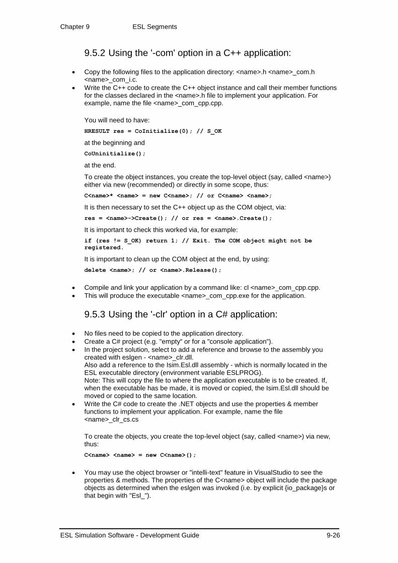
Chapter 9 ESL Segments
ESL Simulation Software - Development Guide 9-26
9.5.2 Using the '-com' option in a C++ application:
Copy the following files to the application directory: <name>.h <name>_com.h <name>_com_i.c.
Write the C++ code to create the C++ object instance and call their member functions for the classes declared in the <name>.h file to implement your application. For example, name the file <name>_com_cpp.cpp.
You will need to have:
HRESULT res = CoInitialize(0); // S_OK
at the beginning and
CoUninitialize();
at the end.
To create the object instances, you create the top-level object (say, called <name>) either via new (recommended) or directly in some scope, thus:
C<name>* <name> = new C<name>; // or C<name> <name>;
It is then necessary to set the C++ object up as the COM object, via:
res = <name>->Create(); // or res = <name>.Create();
It is important to check this worked via, for example:
if (res != S_OK) return 1; // Exit. The COM object might not be
registered.
It is important to clean up the COM object at the end, by using:
delete <name>; // or <name>.Release();
Compile and link your application by a command like: cl <name>_com_cpp.cpp.
This will produce the executable <name>_com_cpp.exe for the application.
9.5.3 Using the '-clr' option in a C# application:
No files need to be copied to the application directory.
Create a C# project (e.g. "empty" or for a "console application").
In the project solution, select to add a reference and browse to the assembly you created with eslgen - <name>_clr.dll. Also add a reference to the Isim.Esl.dll assembly - which is normally located in the ESL executable directory (environment variable ESLPROG). Note: This will copy the file to where the application executable is to be created. If, when the executable has be made, it is moved or copied, the Isim.Esl.dll should be moved or copied to the same location.
Write the C# code to create the .NET objects and use the properties & member functions to implement your application. For example, name the file <name>_clr_cs.cs
To create the objects, you create the top-level object (say, called <name>) via new, thus:
C<name> <name> = new C<name>();
You may use the object browser or "intelli-text" feature in VisualStudio to see the properties & methods. The properties of the C<name> object will include the package objects as determined when the eslgen was invoked (i.e. by explicit {io_package}s or that begin with "Esl_").

Chapter 9 ESL Segments
ESL Simulation Software - Development Guide 9-27
You may run the application directly in the C# project to debug it, or create an executable to run independently.
An alternative to using C# project in VisualStudio is to use the 'csc' C# compiler directly.
Copy the <name>_clr.dll assembly (created via eslgen -clr) and the 'Isim.Esl.dll' assembly (from the ESL executable directory) to the application directory.
Having created a C# program (say <program>.cs) that uses the <name>_clr.dll assembly, compile it with a command like:
csc /reference:<name>_clr.dll,Isim.Esl.dll <program>.cs
Examples
The ...\esl\examples directory includes the source files for applications developed for the 'embseg.esl' example when DLLs for it are generated with the eslgen command (with 'embcom' specified as io_package, that is, 'eslgen -dll embseg embcom'). We recommend that you copy the files to separate directories to do the generations, and to try the example applications.
The example source file that uses the 'embseg_dll.dll' (generated by the '-dll' option) is:
embprg_dll_c.c - C source file. (Build this example with 'cl embprg_dll_c.c embseg_dll.lib'.)
The example source file that uses the 'embseg_com.dll' (generated by the '-com' option) is:
embprg_com_cpp.cpp - C++ source file.
The example source file that uses the 'embseg_clr.dll' (generated by the '-clr' option) is:
embprg_clr_cs.cs - C# source file. (You may build this example with 'csc /r:embseg_clr.dll,Isim.Esl.dll embprg_clr_cs.cs'.)
You may also care to look at the example that illustrate the use of two instances of the same embedded segment - the sineprg_clr_cs.cs C# program which uses the sineseg.esl example.

Chapter 10 Steady-State Analysis
ESL Simulation Software - Development Guide 10-1
CHAPTER 10
10 Steady-State Analysis This section introduces steady-state analysis support, which provides steady-state "finders", linearization, Eigenvalue determination, and parameter optimization.
Contents:
Introduction
The ANALYSIS Region
The TRIM Statement
the LINEARIZE Statement
the EIGENVALUE Statement
The ANALYSIS MODEL Call
Steady-State Algorithms
Optimization
Two Link Robot Arm Example
10.1 Introduction Whether or not a system is linear depends on whether or not it satisfies the principles of superposition:
𝐹(𝑥1 + 𝑥2) = 𝐹(𝑥1) + 𝐹(𝑥2)
and Homogenity:
𝐹(𝜏𝑥) = 𝜏𝐹(𝑥)
Most real systems are highly non-linear. However, it is often desirable to consider their operation over a limited range about a steady-state position. In such cases the system may be approximated by a linear model, expressed in state-space form as:
𝒙′ = 𝑨𝑥 + 𝑩𝑢𝒚′ = 𝑪𝑥 + 𝑫𝑢
where:
A is the system matrix,
B is the input matrix,
C is the output matrix,
D is the input to output relationship (often zero),
u is the input vector,
y is the output vector and
x is the state vector
These equations will be valid only in those regions of linearity which are centred around the steady-state position.
It is often desirable in modelling to obtain such a linear approximation of the system model at a steady-state position, so that linear analysis and design techniques may be applied.
To locate a steady-state position, a TRIM statement is provided which uses one of two alternative steady-state algorithms to locate the point at which specified derivatives are zero. To calculate the A, B, C and D matrices described above, a LINEARIZE statement is used. The LINEARIZE statement invokes a perturbation technique to determine the linear model. Also provided is an EIGENVALUE statement which allows the eigenvalues of the linearized model to be calculated.

Chapter 10 Steady-State Analysis
ESL Simulation Software - Development Guide 10-2
These facilities are provided by the inclusion of an ANALYSIS region in the model subprogram. The ANALYSIS region, which appears at the end of the MODEL following the TERMINAL region (if present), may contain procedural code including one TRIM and one LINEARIZE statement. The EIGENVALUE statement is a general procedural code statement and, although typically used in the ANALYSIS region, may appear in any procedural code region. The TRIM and LINEARIZE statements specify the steady-state and linearization requirements respectively. A special model call is made to invoke the ANALYSIS region by setting the integration algorithm reserved variable, ALGO, to an appropriate value. Normal calls to the model ignore the ANALYSIS region. Related features are the ESL RESUME and RESTART statements, (ESL Run Control), which allow a model to be continued (resumed), or restarted, from the state it had reached on completion of the preceding call. This is a general feature which in the present context may be used to invoke a linearization having first run the model to a steady-state condition, or alternatively, to request a run from the steady-state resulting from execution of the TRIM statement. The latter operation may be attempted to verify the steady-state condition. These facilities are described in the following sections.
10.2 The ANALYSIS Region To find a steady-state of a model or to linearize it, an ANALYSIS region is included as the last region of the MODEL subprogram. The region is specified by the keyword ANALYSIS.
MODEL MOD1;
...
INITIAL
...
DYNAMIC
...
TERMINAL
...
ANALYSIS
... analysis region
...
END MOD1;
The ANALYSIS region is a procedural code region and may contain any procedural statements (such as PRINT, READ, assignments etc). In particular it may contain only one TRIM and/or one LINEARIZE statement.
Note that an ANALYSIS region may only appear in a MODEL subprogram. It may not appear in a SUBMODEL or SEGMENT.
10.3 The TRIM Statement The TRIM statement specifies the steady-state requirements.
The problem of finding a steady-state is essentially: "given the steady-state values of certain state variables and/or required inputs, find the remaining state and/or input values consistent with the steady-state condition", that is:
Given system inputs find the values for state variables which make the derivatives zero, or
given values for the state variables find values of inputs which make the derivatives zero, or
given some state variables and some inputs - find the remaining state variables and inputs which make the derivatives zero.
The known variable values are set in the initial region of the model. The TRIM statement specifies those derivatives which must be zero at the steady-state (the derivative vector) and

Chapter 10 Steady-State Analysis
ESL Simulation Software - Development Guide 10-3
an equal number of states and/or inputs, the values of which are to be found (the control vector). The form of the statement is as follows:
TRIM [ control_vector ] := [ derivative_vector ] ;
where:
control_vector is a list of states and/or inputs.
derivative_vector is a list of derivatives.
The states, inputs and derivatives may be scalar variables, one dimensional arrays or a mixture of both.
Example
TRIM [ x,y,ARR ] := [ BRR',z',x' ];
Where:
x, y, and z are scalar variables and
ARR and BRR are arrays.
Note that the total number of scalar variables and array elements must be the same in the control vector and the derivative vector, but that the order is not important.
In terms of ESL's usage classification of simulation variables, the control variables may be classified as states or parameters (a variable set in the INITIAL region and not subsequently changed). The derivatives may be any variable with class algebraic.
The TRIM statement effectively identifies a subset of the dynamic region as being a set of non-linear algebraic equations to be solved. A value for the control vector must be found which forces the derivative vector to zero.
10.4 The LINEARIZE Statement For the required steady-state condition, the linearized model may be expressed in state-space form as:
𝒙′ = 𝑨𝑥 + 𝑩𝑢𝒚′ = 𝑪𝑥 + 𝑫𝑢
where:
x is the state vector,
u is the input vector and
y is the output vector.
Note that here x, u, and y are not the absolute values of the state, input and output vectors, but deviations from their steady-state values.
The LINEARIZE statement specifies the names of arrays to hold the A and B matrices, the state vector and the input vector. Optionally, arrays to hold the C and D matrices and the output vector may also be specified. The arrays for the state-space matrices must have been declared and have appropriate dimensions. The form of the LINEARIZE statement is:
LINEARIZE A_matrix, B_matrix := [state_vector],[input_vector];
if the state equation only is required, or:
LINEARIZE A_matrix, B_matrix := [state_vector], [input_vector]
C_matrix, D_matrix := [output_vector];
if both state and output equations are required,
where:
A_matrix, B_matrix, C_matrix and D_matrix are the names of arrays to
hold the state-space A, B, C, and D matrices.
state_vector is a list of states,

Chapter 10 Steady-State Analysis
ESL Simulation Software - Development Guide 10-4
input_vector is a list of inputs and
output_vector is a list of outputs.
As with the TRIM statement, the states, inputs and outputs may be scalar variables, one dimensional arrays or a mixture of both.
Example:
LINEARIZE A, B := [ x, z, BRR ], [ URR, u1, u2]
C, D := [ y1, y2 ];
Where:
x, z, u1, u2, y1, y2 are scalar variables and
BRR and URR are arrays.
10.5 The EIGENVALUE Statement An n x n matrix A has an eigenvector x and corresponding eigenvalue λ if:
𝑨𝒙 = 𝜆𝒙
It follows that the eigenvalues are the n roots of the characteristic equation:
𝑑𝑒𝑡|𝑨 − 𝜆𝑰|
The eigenvalues of the state-space A matrix are of particular importance since they characterize the dynamic performance of the linearized model.
The EIGENVALUE statement is provided to determine the eigenvalues of a square matrix and has the following form:
EIGENVALUE L := A;
where:
A is the real n x n matrix whose eigenvalues are to be determined and
L is a real n x 2 array to hold the eigenvalues.
On return from the statement, L(1..n, 1) will contain the real parts of the eigenvalues, and L(1..n, 2) will contain the imaginary parts (if the eigenvalues are complex).
Typically the EIGENVALUE statement will be positioned in the ANALYSIS region to determine the eigenvalues of the state-space A matrix following a TRIM and LINEARIZE statement. For example:
TRIM [x1, x2] := [x1', x2'];
LINEARIZE A,B := [x1, x2], [input];
EIGENVALUE L := A;
Note that as with the A and B matrices, the L array must have been previously declared and have correct dimensions.
The EIGENVALUE statement is a general procedural code statement, and not therefore restricted to the ANALYSIS region, and may be used to determine the eigenvalues of any real square matrix.
10.6 The ANALYSIS MODEL Call The steady-state and linearize requirements specified by appropriate TRIM and LINEARIZE statements placed in the ANALYSIS region are activated by calling the model with ALGO set to LIN1 or LIN2 from the experiment region. The effect of this special MODEL call is first to carry out an initialization pass of the MODEL including any SUBMODELs it might call. Control then passes to the ANALYSIS region where, on encountering a TRIM or LINEARIZE

Chapter 10 Steady-State Analysis
ESL Simulation Software - Development Guide 10-5
statement, appropriate DYNAMIC region code passes are made as necessary to accomplish the specified operations.
The alternative values of ALGO (LIN1 or LIN2) specify either a Newton-Raphson, or a Simplex optimization algorithm to be used by the TRIM statement to locate the steady-state. The same perturbation algorithm is invoked by the LINEARIZE statement irrespective of which value of ALGO is used.
Example:
Experiment
...
ALGO := LIN1; or ALGO := LIN2;
MOD1;
...
The analysis region may contain PRINT statements to communicate the computed steady-state values and the resultant state-space matrices. Alternatively these results may be passed back to the experiment region as model arguments.
The state-space matrices may, of course, be written in an appropriate form to a file to be analyzed at a later time using a proprietary linear analysis package.
A complete example of using the ESL linearization facilities is given at the end of this section.
10.7 Steady-State Algorithms Currently ESL supports two routines for determining a steady-state condition, the Newton-Raphson (LIN1) and the Simplex (LIN2). These are selected by setting the ALGO variable to LIN1 or LIN2 in the Experiment region prior to calling the MODEL, or in the model's INITIAL region. Note that during these processes discontinuity states are frozen at their initial values.
LIN1 - Newton-Raphson Algorithm
This approach uses a standard iterative Newton-Raphson formula to solve the set of non-linear algebraic equations inferred by the TRIM statement.
If F(x) = 0 is the set of equations to be solved (F(x) is the derivative vector, and x is the control vector). Given an initial value for the control vector, x1, improved values are found using the formula:
𝒙𝑛+1 = 𝒙𝑛 − 𝑱−1𝑭(𝒙) 𝑓𝑜𝑟 𝑛 = 1,2,…𝑢𝑛𝑡𝑖𝑙 𝑎𝑙𝑔𝑜𝑟𝑖𝑡ℎ𝑚 𝑐𝑜𝑛𝑣𝑒𝑟𝑔𝑒𝑠
J is the Jacobian matrix (𝜕𝑭𝜕𝒙⁄ ) and is determined using perturbation techniques.
LIN2 - Simplex Algorithm
There are situations when the use of the Newton-Raphson method fails to find a steady-state because a singular Jacobian matrix occurs at some point in the iterations. In such situations, an alternative Simplex optimization algorithm may be invoked (see the paper by J A Nelder and R Mead in The Computer Journal, 1965, Vol 7, page 308)
For a given function:
𝑭(𝒙) 𝑤ℎ𝑒𝑟𝑒 𝒙 = [𝑥1, 𝑥2, … 𝑥𝑛]𝑇
the Simplex algorithm will attempt to find a value for x which will minimize F(x). In the present context, x is the control vector as specified in the TRIM statement and F(x) is calculated as the sum of squares of the derivative vector elements. Thus, use of the Simplex algorithm computes a control vector which minimizes the derivative vector. If the minimized derivative vector is zero (or approximately zero) then a steady-state of the model has been found.
Warning: As with any optimization algorithm, there is no guarantee that the global minimum of the function will be located. The algorithm may come to rest on any one of a number of possible local minima. It is therefore important to check a true steady-state has been found when using the Simplex algorithm.

Chapter 10 Steady-State Analysis
ESL Simulation Software - Development Guide 10-6
Algorithm description
At the starting point in the n-dimensional space of the control vector, the Simplex algorithm requires the construction of an initial simplex, that is, a geometrical figure consisting of n+1 vertices. Thus, in two dimensions the simplex is a triangle; in three dimensions a tetrahedron and so on. The algorithm computes the value of F(x) at each of the vertices of the initial simplex, and defines a second simplex by reflecting the worst vertex (the one having the largest value of F(x)) through the opposite side. This manoeuvre is repeated as the simplex progresses through n-dimensional space towards the minimum. The size and shape of the simplex is automatically changed by the algorithm allowing long or short steps to be taken in each direction, depending on the manner in which F(x) varies.
The Simplex algorithm is not renowned for its efficiency in terms of function evaluations, but it is robust and considered a suitable general purpose algorithm able to cope with a wide range of nonlinear models.
Initialisation
The size of the initial simplex should be chosen in accordance with the scale or order of magnitude of the control variables (elements of x) and the anticipated proximity of their initial values to the steady-state. In order to provide a simple means of specifying the size of the initial simplex, the reserved variable CINT (normally the communication interval in a simulation) is given a different meaning and used with the initial value of the control vector in the following manner:
If
𝒙0 = [𝑥1, 𝑥2,… 𝑥𝑛]𝑇
is the starting point (initial value of the control vector), then the remaining n initial simplex vertices are computed using:
𝒙𝑖 = 𝒙0 + 𝐷𝑖𝒖𝑖 𝑓𝑜𝑟 𝑖 = 1…𝑛
where the ui's are the n unit vectors, that is, the initial simplex has an edge of length Di along the i
th dimension. Di is calculated using:
𝐷𝑖 = {𝐶𝐼𝑁𝑇 𝑖𝑓 𝑥𝑖 = 0.0𝐶𝐼𝑁𝑇 × 𝑥𝑖 𝑖𝑓 𝑥𝑖 ≠ 0.0
If the initial value of a control variable is non-zero, then the simplex side length, in the direction of that variable, is the initial value multiplied by CINT. If, however, the initial value of a control variable is zero, then the simplex side length in that direction is taken as CINT.
Alternatively, the Reserved variable, OP_STP, may be used to establish an initial value for the size of the simplex. To employ OP_STP, instead of CINT, simply change the value of OP_STP from its default value of zero prior to optimization or linearization.
10.8 Optimization A general user interface is provided to the Simplex optimization algorithm used by the LIN2 steady-state option. This allows dynamic optimization of ESL models to be undertaken. For example, it may be necessary to select the gains of a PID controller to achieve optimum dynamic response of a control system. In this case, a model of the control system would be formulated with a suitable performance function as a single output, and the PID controller gains as input arguments. The model is called in a special manner using an OPTIMIZE statement from the experiment region. Repeated runs of the model are automatically made under the control of the optimization algorithm, which varies the model arguments in order to minimize the performance function. On return from the OPTIMIZE statement, the model performance function output will be set to the minimum value achieved, and the input arguments to their corresponding optimum values.
The OPTIMIZE statement may also be used to minimize an algebraic function of several variables. This is achieved by writing the function within an ESL procedure, with the function

Chapter 10 Steady-State Analysis
ESL Simulation Software - Development Guide 10-7
value as the first argument (output) and the variables as the following arguments (inputs). The procedure is then called through the OPTIMIZE statement in a similar manner to an ESL model.
The OPTIMIZE statement
The form of the OPTIMIZE statement is:
OPTIMIZE subprog_name(cost := par1, par2, ... );
where:
subprog_name is the name of the ESL model or procedure to be
optimized,
cost is the performance function output to be minimized and
par1, par2, .... are the input arguments.
The OPTIMIZE argument list must match exactly that of the subprogram definition and all the arguments must be of type real. Further, the input arguments must be variables, not expressions, and be given initial values before the optimization call. For example:
STUDY
MODEL CONTROLLER(REAL: cost := REAL: g1, g2, g3);
......
......
END CONTROLLER;
-- EXPERIMENT
REAL: perform, gain1, gain2, gain3;
gain1 := 0.1; gain2 := 0.1; gain3 := 0.2;
OPTIMIZE CONTROLLER(perform := gain1, gain2, gain3);
PRINT "performance function", perform;
PRINT "optimum gains", gain1, gain2, gain3;
END_STUDY
10.9 Two Link Robot Arm Example Robot arm
To illustrate the steady-state and linearization features described above, we consider a model of a two link robot arm assembly. The model is highly nonlinear and the problem is to determine an applied torque required to achieve a given steady-state condition, and hence obtain a linearized model at that steady-state. The arrangement of the robot arm is shown in the figure above.

Chapter 10 Steady-State Analysis
ESL Simulation Software - Development Guide 10-8
The model
Theta1 defines the angular displacement of the first link with respect to the vertical. Theta2 defines the angular displacement of the second link with respect to the first. Quantities (2*l1), m1 and J1 are the length, mass and moment of inertia respectively of the first link and (2*l2), m2 and J2 similar quantities for the second. F1 and F2 are viscous friction terms associated with the two joints. Tau1 and Tau2 are torques applied externally at the two joints. Motion in the vertical plane only is considered. The arrangement may be described by the following equations:
Tau1 = a*Theta1'' + b*Theta2'' + c
Tau2 = d*Theta1'' + e*Theta2'' + f
where:
a = J1 + J2 + 4*m2*(l1)2 + 4*m2*l1*l2*COS(Theta2)
b = J2 + 2*m2*l1*l2*COS(Theta2)
c = -4*m2*l1*l2*SIN(Theta2)*Theta1'*Theta2'
-2*m2*l1*l2*SIN(Theta2)*(Theta2')2
-m2*l2*g*SIN(Theta1+Theta2) - 2*m2*l1*g*SIN(Theta1)
-m1*l1*g*SIN(Theta1) + F1*Theta1'
d = J2 + 2*m2*l1*l2*COS(Theta2)
e = J2
f = -m2*l2*g*SIN(Theta1+Theta2) + 2*m2*l1*l2*SIN(Theta2)
*(Theta1')2 +F2*Theta2'
These equations may be written in matrix form as:
TAU = A * THETA'' + B
where:
TAU = [Tau1 Tau2]T
THETA = [Theta1 Theta2]T
A = |a b|
|d e|
B = [c f]T
Hence the system may be described by the second order differential equation:
THETA'' = A-1 (TAU - B)
Steady-state and linearization
It is required to find the two torques, Tau1 and Tau2, which result in the steady-state condition:
Theta1 = 45 degrees
Theta2 = 0 degrees
This is an exacting requirement since it represents an unstable condition; the slightest perturbation from the steady-state will either cause the system to flip to a stable condition with Theta1 equal to 135 degrees and Theta2 equal to zero degrees, or cause the arms to rotate continuously.
Once in the steady-state, the following linearized model is required:
|th1' | |th1 | |tau1|
|th2' | = AA |th2 | + BB | |
|th1''| |th1'| |tau2|
|th2''| |th2'|
ESL program
An ESL program to achieve the required steady-state and linearization requirements is listed below. The following notes provide an explanation of the program structure and operation.
The model ROBOTARM implements the mathematical model described above. Vectors are used to represent Theta (th(2)) and Tau (tau(2)). Hence the system differential equation is expressed as:
th'' := INV(A)*(tau-B);

Chapter 10 Steady-State Analysis
ESL Simulation Software - Development Guide 10-9
Note that the use of the procedural block to set individual elements of the matrices A and B.
For the steady-state requirement, Tau1 and Tau2 form the control vector (we are seeking values for these variables consistent with the steady-state condition). Similarly, Theta1'' and Theta2'' form the derivative vector (which must be zero at the steady-state). Thus the TRIM statement in the analysis region takes the form:
TRIM [tau] := [th''];
For the linearized model, matrices AA(4,4) and BB(4,2) are declared. Theta1, Theta2, Theta1', Theta2' form the state vector and Tau1, Tau2 the input vector. The LINEARIZE statement is therefore:
LINEARIZE AA, BB := [th,th'], [tau];
Further statements are included in the analysis region to print out the steady-state torque, and the values of the AA and BB matrices.
The model is written so that values specifying the steady-state (Theta1, Theta2, Theta1' and Theta2') and an initial guess at the torque (Tau1 and Tau2) are passed as arguments. These are the input arguments th0(2), thd0(2) and torque(2). The resultant steady-state torque is returned as the output argument of the model, sstrq(2).
In the experiment region of the program, the steady-state values of the state variables and the initial value of torque are set. The model is then called with ALGO equal to LIN1 to perform an analysis region pass.
Following the analysis pass, which will establish the steady-state and linearized model, provision is made in the experiment to perform a normal simulation from the established steady-state condition through the use of the RESUME statement. The purpose of this simulation run is to demonstrate that the steady-state has been successfully found by generating a plot of Theta1 and Theta2. It should be observed that Theta1 and Theta2 remain constant throughout the run. The program then enters a loop in which normal simulation runs are made using values of torque entered by the user. It will be observed that by entering values of torque only slightly different from the calculated steady-state values will cause the robot arm to flip into a stable state, or rotate continuously.
Results
The values of the steady-state torque and the linearized model matrices, as printed by the program are:
Steady-state tau1, tau2: -0.090836495 -0.017792713
State-space arrays AA, BB :
0.00000E+00 0.00000E+00 1.0000 0.00000E+00
0.00000E+00 0.00000E+00 0.00000E+00 1.0000
42.452 -21.221 -8.6677 20.572
-59.939 90.615 20.491 -71.329
0.00000E+00 0.00000E+00
0.00000E+00 0.00000E+00
871.64 -2060.0
-2060.6 7142.7

Chapter 10 Steady-State Analysis
ESL Simulation Software - Development Guide 10-10
Robot arm results
Graphs of Theta1 and Theta2, as displayed by the Post Run Plot option of the ISE Display Manager from the prepare file are shown in the figure above. Run 1 corresponds to the steady-state, showing Theta1 constant at 45 degrees and Theta2 constant at zero degrees. Run 2 was obtained using torques of:
Tau1 = -0.09083640 Tau2 = -0.01779271
Program listing - distributed file robotarm.esl
STUDY
-- Two link robot arm example.
-- The model represents two dimensional motion of a two link robot
-- arm. th1 is the angular position of the first link with respect
-- to the vertical; th2 is the position of the second link relative
-- to the first. m1, l1, J1 are the mass, length and inertia of the
-- first link; m2, l2, J2 are similar constants of the second.
-- The matrix C represents viscous friction terms.
-- tau1 is the absolute torque applied to the first link; tau2 is
-- the torque applied to the second link relative to the first.
-- Inputs to the model are: the constant applied torque (torque)
-- and initial values for th1, th2 (th0) and th1',th2' (thd0).
--
MODEL ROBOTARM(REAL:sstrq(2):=REAL:torque(2),th0(2),thd0(2));
REAL:tau(2),th(2),Theta(2),thd(2),A(2,2),B(2);
CONSTANT REAL:m1/0.052/,m2/0.019/,J1/9.26E-4/,J2/4.40E-4/,
l1/0.117/,l2/0.135/,g/9.81/,F1/0.01/,F2/0.01/;
REAL:AA(4,4),BB(4,2);
INITIAL
-- Initialize input (control) and states
tau := torque;
th := th0;
th' := thd0;
DYNAMIC
-- The following statement is necessary since the forms
-- th'(1) or th(1)' are not allowed
thd := th';
PROCEDURAL(A,B := th,thd);
-- This procedural block is necessary to assign values to
-- matrix elements
A(1,1) := J1+J2+4.0*m2*l1*l1+4.0*m2*l1*l2*COS(th(2));
A(1,2) := J2+2.0*m2*l1*l2*COS(th(2));
A(2,1) := J2+2.0*m2*l1*l2*COS(th(2));
A(2,2) := J2;
B(1) := -2.0*m2*l1*l2*SIN(th(2))*thd(2)*(2.0*thd(1)+thd(2))
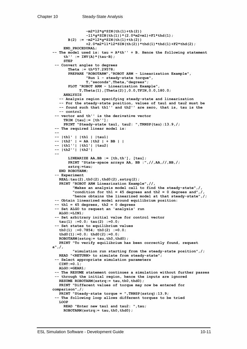
Chapter 10 Steady-State Analysis
ESL Simulation Software - Development Guide 10-11
-m2*l2*g*SIN(th(1)+th(2))
-l1*g*SIN(th(1))*(2.0*m2+m1)+F1*thd(1);
B(2) := -m2*l2*g*SIN(th(1)+th(2))
+2.0*m2*l1*l2*SIN(th(2))*thd(1)*thd(1)+F2*thd(2);
END_PROCEDURAL;
-- The model used is: tau = A*th'' + B. Hence the following statement
th'' := INV(A)*(tau-B);
STEP
-- Convert angles to degrees
Theta := th*57.29578;
PREPARE "ROBOTARM","ROBOT ARM - Linearization Example",
"Run 1 - steady-state torque",
T,"seconds",Theta,"degrees";
PLOT "ROBOT ARM - Linearization Example",
T,Theta(1),[Theta(2)],0.0,TFIN,0.0,180.0;
ANALYSIS
-- Analysis region specifying steady-state and linearization
-- For the steady-state position, values of tau1 and tau2 must be
-- found such that th1'' and th2'' are zero, that is, tau is the
-- control
-- vector and th'' is the derivative vector
TRIM [tau]:= [th''];
PRINT "Steady-state tau1, tau2: ",TRNSP(tau):13.9,/;
-- The required linear model is:
--
-- |th1' | |th1 | |tau1|
-- |th2' | = AA |th2 | + BB | |
-- |th1''| |th1'| |tau2|
-- |th2''| |th2'|
--
LINEARIZE AA,BB := [th,th'], [tau];
PRINT "State-space arrays AA, BB :",//,AA,//,BB,/;
sstrq:=tau;
END ROBOTARM;
-- Experiment
REAL:tau(2),th0(2),thd0(2),sstrq(2);
PRINT "ROBOT ARM Linearization Example",//,
"Makes an analysis model call to find the steady-state",/,
"condition for th1 = 45 degrees and th2 = 0 degrees and",/,
"hence obtains the linearized model at that steady-state",/;
-- Obtain linearized model around equilibrium position:
-- th1 = 45 degrees, th2 = 0 degrees
-- Set ALGO to request an 'analysis' run
ALGO:=LIN1;
-- Set arbitrary initial value for control vector
tau(1) :=0.0; tau(2) :=0.0;
-- Set states to equilibrium values
th0(1) :=0.7854; th0(2) :=0.0;
thd0(1):=0.0; thd0(2):=0.0;
ROBOTARM(sstrq:= tau,th0,thd0);
PRINT "To verify equilibrium has been correctly found, request
a",/,
"simulation run starting from the steady-state position",/;
READ "<RETURN> to simulate from steady-state";
-- Select appropriate simulation parameters
CINT:=0.1;
ALGO:=GEAR1;
-- The RESUME statement continues a simulation without further passes
-- through the initial region, hence the inputs are ignored
RESUME ROBOTARM(sstrq:= tau,th0,thd0);
PRINT "Different values of torque may now be entered for
comparison",/;
PRINT "Steady-state torque = ",TRNSP(sstrq):13.9;
-- The following loop allows different torques to be tried
LOOP
READ "Enter new tau1 and tau2: ",tau;
ROBOTARM(sstrq:= tau,th0,thd0);

Chapter 10 Steady-State Analysis
ESL Simulation Software - Development Guide 10-12
END_LOOP;
END_STUDY

Chapter 11 ESL Run Control
ESL Simulation Software - Development Guide 11-1
CHAPTER 11
11 ESL Run Control This section describes how an ESL simulation execution may be controlled when using the Interpreter or a Translator generated program. The features described here allow the user to change the course of a simulation without changing the basic ESL program. They include: user interaction with program; restarting or continuing an ESL simulation run; using the "snapshot" facility to restart or continue a simulation; changing ESL parameters at the start of execution and during the course of execution.
Contents:
INTERACT Control
Simulation Driver Files
RESUME and RESTART
Snapshot Support
11.1 INTERACT Control The INTERACT service provides a means of monitoring progress and examining the values of user variables. It gives the user the ability to change variables, continue, restart or quit the simulation. In short, it provides a monitoring, testing and debugging facility, and also a simple way of changing the course of the simulation without having to program changes in ESL source code.
The INTERACT service may be invoked either by an explicit INTERACT statement, for example:
INTERACT;
or conditionally, by, for example:
if t >= t_interact then INTERACT; end_if;
The Interact service may be explicitly invoked by an INTERACT statement in the user program, or implicitly invoked in a number of ways. Command line parameters to specify simulation execution using a "snapshot" or "simulation driver file" (-s, -sc and -drv), are described later in this section, and cause the Interact service to be invoked immediately at the start of a program.
The Interactive service also may be invoked by use of the Break key sequence (Ctrl + Break on a PC, Ctrl + C on most other systems). ESL run-time control takes different actions depending on the number of times the Break key is pressed. During a simulation run:
Entering Break once will cause the Interact service to be entered at the end of a model or segment communication region.
Entering Break twice (before ESL has reached a communication point), will cause the Interact service to be entered after a step region has been computed.
Entering Break three times (before ESL has reached a step or communication point) will be treated as an "abort" break, and cause the Interact service to be entered as soon as possible (with the Interpreter this is immediate). In this case the program is not allowed to continue from the Interact - a restart is the only execution option.
During Linearization a single Break invokes the interactive service.
The ESL keyboard READ is not over-sensitive to a Break; it causes the current input to be deleted (as ^U or Esc), but it does not abort the reading operation. If new valid user input occurs the Break is ignored completely, but if Return/Enter is pressed immediately after the
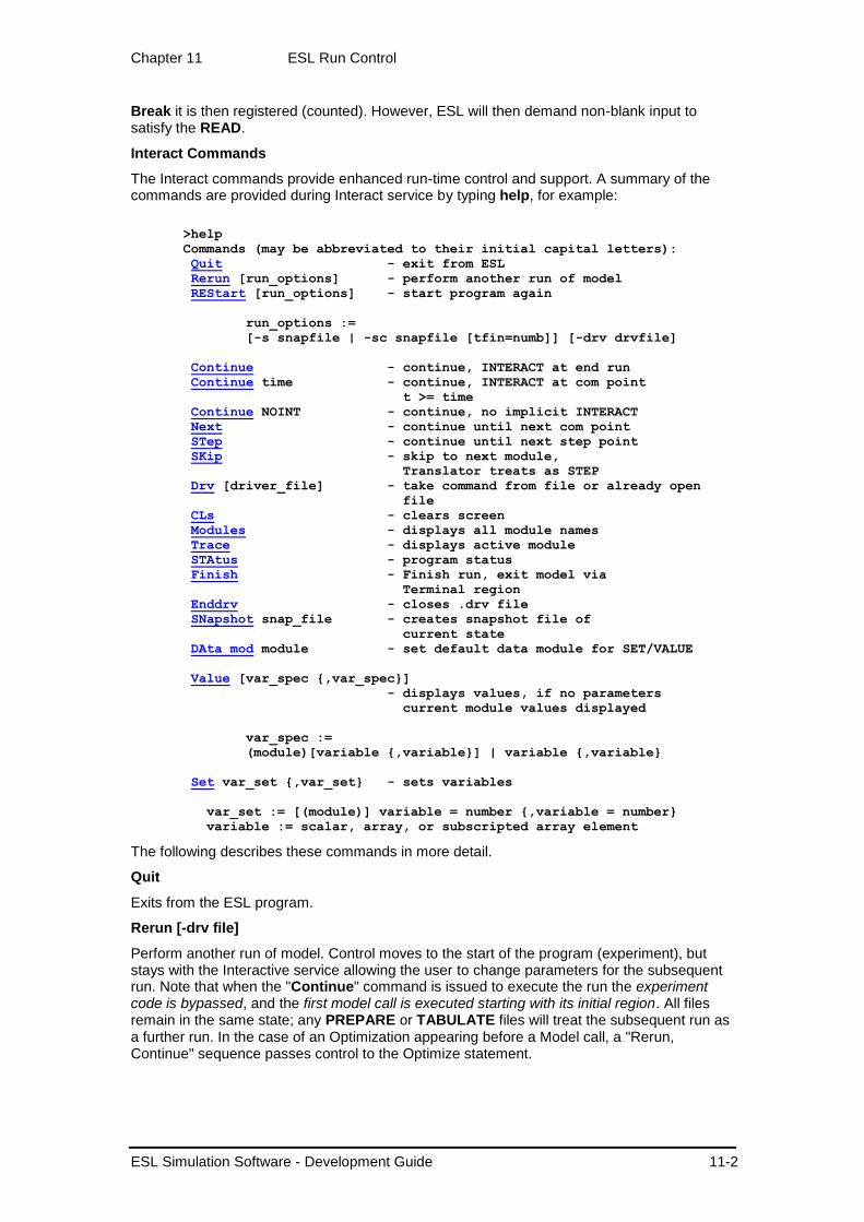
Chapter 11 ESL Run Control
ESL Simulation Software - Development Guide 11-2
Break it is then registered (counted). However, ESL will then demand non-blank input to satisfy the READ.
Interact Commands
The Interact commands provide enhanced run-time control and support. A summary of the commands are provided during Interact service by typing help, for example:
>help
Commands (may be abbreviated to their initial capital letters):
Quit - exit from ESL
Rerun [run_options] - perform another run of model
REStart [run_options] - start program again
run_options :=
[-s snapfile | -sc snapfile [tfin=numb]] [-drv drvfile]
Continue - continue, INTERACT at end run
Continue time - continue, INTERACT at com point
t >= time
Continue NOINT - continue, no implicit INTERACT
Next - continue until next com point
STep - continue until next step point
SKip - skip to next module,
Translator treats as STEP
Drv [driver_file] - take command from file or already open
file
CLs - clears screen
Modules - displays all module names
Trace - displays active module
STAtus - program status
Finish - Finish run, exit model via
Terminal region
Enddrv - closes .drv file
SNapshot snap_file - creates snapshot file of
current state
DAta_mod module - set default data module for SET/VALUE
Value [var_spec {,var_spec}]
- displays values, if no parameters
current module values displayed
var_spec :=
(module)[variable {,variable}] | variable {,variable}
Set var_set {,var_set} - sets variables
var_set := [(module)] variable = number {,variable = number}
variable := scalar, array, or subscripted array element
The following describes these commands in more detail.
Quit
Exits from the ESL program.
Rerun [-drv file]
Perform another run of model. Control moves to the start of the program (experiment), but stays with the Interactive service allowing the user to change parameters for the subsequent run. Note that when the "Continue" command is issued to execute the run the experiment code is bypassed, and the first model call is executed starting with its initial region. All files remain in the same state; any PREPARE or TABULATE files will treat the subsequent run as a further run. In the case of an Optimization appearing before a Model call, a "Rerun, Continue" sequence passes control to the Optimize statement.

Chapter 11 ESL Run Control
ESL Simulation Software - Development Guide 11-3
Restart [run_options]
Restarts the program completely. The run_options are any allowed command line parameters which may be used to start an ESL execution. All files are closed.
Continue [options]
The Continue command is the means of instructing the program to "continue" execution. Its basic use, without qualifying parameters, simply allows the simulation to continue. Even this simple form of the command has the additional property of re-invoking the Interact service at the end of the current or subsequent simulation run.
The Continue noint command will cause the program to continue, but not automatically Interact, as occurs with the other forms of Continue.
The Continue 12.0 form of the command will cause the simulation to continue until the communication point where T >= 12.0, when the Interact service will be re-invoked. If necessary TFIN is automatically modified (to 12.0) to extend the run. This command may be issued at the end of a run (when Interact has been implicitly invoked by previous use of a Continue) to extend the simulation. After a simulation run is complete, and control has passed to the experiment, this command may not be issued (error given). It may be used, however, after a Rerun/Restart command when control has been passed to the start of the program, and a new run is to be undertaken.
Next
The command Next is similar to a Continue, and will cause the simulation to proceed to the next communication point. Once control has been passed to the experiment, after a run, this command may not be used until after a Restart/Rerun command has been issued.
Step
The command Step is similar to a Next, and will cause the simulation to proceed to the next step point. Once control has been passed to the experiment, after a run, this command may not be used until after a Restart/Rerun command has been issued.
Skip
With the Interpreter Skip continues the execution until the next module is encountered, and with the Translator continues execution until next step point is reached. Primarily used for debugging purposes with Interpreter, where repeated Skip commands should eventually pass control to the module of interest.
Drv [driver_file]
The Drv command allows Interact commands to be taken from the specified driver file (.drv extension). See Simulation Driver Files.
Cls
Clears the screen.
Modules
Displays the names of package and Code modules.
Trace
Displays name of the currently active code module, and for the Interpreter, the modules which called the current module.
Status
Presents a message indicating the status of the simulation and the Interact service.
Finish
When control has passed to the INTERACT service during (or at the end) of a simulation run, the Finish command will cause: the run to be immediately terminated; the Terminal region executed; and a return to the experiment. In other contexts it is equivalent to a Continue.
Enddrv

Chapter 11 ESL Run Control
ESL Simulation Software - Development Guide 11-4
Closes the .drv file when Pause, or a Break interaction, is active.
Snapshot snap_file
Creates snapshot file of current state of the simulation, normally used at end of a run. See Snapshot Support on using snapshots to start an execution.
Data_mod module
Sets the default data module for Set/Value commands. The format is:
data_mod module_name
If module_name is omitted, the original Code module is selected as the data module for Set/Value commands.
Value [var_spec {,var_spec}]
Displays values of variables. When used without any options it displays the values of variables in the current code module and any used package modules.
With options it may display all, or specific, variables in any of the code or package modules. For example:
Value (global)kparam,qparam
causes the values of kparam and qparam in module global to be displayed and
Value (global)
displays all variable values in module global. Note that the experiment has the module name EXP$MN.
Subscripted array elements may have their value displayed. For example:
Value ARR(2,3), ARR(2,4)
Arrays of any type, including character, may have their values displayed. The subscripts must be integer numbers, and within the declared range specified in the ESL program.
Set var_set {,var_set}
Sets specified variables to have new values. For example:
Set X=1.0, tfin=5
will set current module's X and Reserved module's TFIN (the Reserved Package is assumed to be used by current module - it is implicitly declared in the Experiment and all modelling modules).
If a variable is not accessible in the current code module, or any packages used by the current module, then it is necessary to explicitly specify the module, for example:
Set (global) kparam=-2.0, qparam=5
will set kparam and qparam located in module global. Note that the experiment has the module name EXP$MN.
Subscripted array elements may have their values set. For example:
Set ARR(2,3)=23.0, ARR(2,4)=24.0
Arrays of any type, including character, may have their values set. The subscripts must be integer numbers, and within the declared range specified in the ESL program.
11.2 Simulation Driver Files A Simulation Driver File (.drv) may be specified to set parameters prior to a simulation, and then to control the simulation. The commands that may appear in a driver file are identical to those available in the Interact service. It may be used in conjunction with a snapshot

Chapter 11 ESL Run Control
ESL Simulation Software - Development Guide 11-5
specification, in which case it takes effect after the snapshot has been processed. For example:
esl -x eslfil -drv driver_file
esl -i eslfil -sc snapfile -drv driver_file
esl -i eslfil -drv
The last example does not use a driver file, but allows the user to interactively enter driver-type commands. The interactive service is invoked immediately at the start of the program.
The driver file sets parameters and then may control the simulation run, and subsequent runs. It is designed to be used with programs with a simple experiment, for example, the benchmark bench5.esl (provided in the library).
-- EXPERIMENT
USE GLOBAL;
REAL: X,Y;
CINT:=0.1;
VANDERPOL (X,Y);
END_STUDY
Note that there is only one statement before the model call, to set CINT, and the model call does not have any input arguments (K is an input to the model declared as a PARAMETER in Package GLOBAL). The model input K could have been an input argument to the model, but this example shows the alternative mechanism of using a Package for this purpose.
The following driver file (bench5.drv) may be used to control the simulation, for example:
set tfin=8.0
set k=1.0
-- start run
continue
-- Perform second run
rerun
set cint=1,nstep=10
set k=2.0
--Interact at T=5
cont 5
Change value of K
set k=6
cont --and complete run
Note that text following "--" is ignored and may be regarded as a comment. This file specifies two runs of the model: the first with K set to 1.0, and TFIN set to 8; the second with K set to 2, CINT to 1, and NSTEP to 10. In addition the second run Interacts at T equal to 5.0 and sets K to 6 before continuing to the end of run.
Driver files may be specified during INTERACT service, using the Drv command.
Driver files may include a Pause command which switches control from the .drv file to the user to allow monitoring or changing data. In the INTERACT service a simple Continue causes the next command to be taken from the .drv file; this is equivalent to a Drv command (with no file specified).
In a .drv file a Pause should normally be followed by an execution command such as Continue, for example:
....
continue 8.0
pause
-- continue to end of run
continue
pause
rerun
....
Note that the line starting with "--" is interpreted as a comment.
During .drv file processing a user Break/Ctrl-C temporarily suspends the .drv file control. A simple Continue continues the simulation with commands being taken from the .drv file at the next scheduled interaction point.

Chapter 11 ESL Run Control
ESL Simulation Software - Development Guide 11-6
The Pause is similar to a user Break/Ctrl-C, in that any subsequent simulation execution command, except a simple Continue, will cause the driver file to be closed and abandoned.
In addition, the INTERACT command "Enddrv will close the .drv file when Pause, or a Break interaction, is active.
Interact commands Next, Step and Skip may now be used to extend a simulation run. If used at the end of run TFIN is increased by the value of CINT. These commands may also be used to start a run.
Embedded simulation may use a .drv file for basic sequential operations (not Rerun/Restart).
11.3 RESUME and RESTART The ESL RESUME and RESTART keywords are prefixed to a MODEL call to cause the model to restart, or resume the last simulation run undertaken by the program.
In this context restart means: start the simulation from the conditions that prevailed when it was last terminated, but with time reset to its initial value (T = TSTART). The simulation bypasses the INITIAL region, and the COMMUNICATION region is executed prior to simulation.
Resume means continue the simulation from the conditions that prevailed when it was last terminated, and with time also continuing from that point (note that TFIN must be increased for this to work). The simulation bypasses the INITIAL region, and also the first COMMUNICATION region before continuing the simulation. For example:
RESUME VANDERPOL(X,Y:=K);
11.4 Snapshot Support A "snapshot" of the state of the system being simulated may be taken for the purpose of starting, or continuing, a simulation from that particular state at some later time. Normally a snapshot will be taken during a simulation run, or the end of a run, and at a point when control has passed to the end of the model communication region.
Taking a snapshot creates a snapshot file to save the state of the simulation, and it may be created by:
(1) Snapshot ESL program statement.
For example:
snapshot snapfile;
or
snapshot;
In the first case a file snapfile.snp is created to contain the present state of the system, and in the second case the user is prompted for the filename. If no file extension is provided a default extension, .snp, is used.
(2) Snapshot Interact command
Commands may be issued during the Interact service to take a snapshot, for example:
snap snapfile
or
snap
The action is the same as that described above, for the snapshot program statement. An Interact snap command may appear in a driver (.drv) file processed either by an executing simulation or ISE.

Chapter 11 ESL Run Control
ESL Simulation Software - Development Guide 11-7
(3) During ISE operation
A snapshot file may be created by clicking the Take Snapshot... button on the control panel, and then specifying the snapshot filename in the Save As window. The same conventions as described above are used for the default extension to the filename.
In each case the snapshot file is a text file containing INTERACT style commands to set user variables to values they had at the time the snapshot was taken. The file also contains comments that specify: the time and date of the snapshot; the ESL Revision number; and the name of the program that generated the snapshot.
The snapshot file may be used to start a simulation run in the following ways:
(1) As a command line parameter
The command line to invoke a simulation execution may have command line parameters to start the simulation from the state which prevailed when a snapshot was taken. For example:
esl -x eslfile -sc snapfile
or
esl -i eslfil -s snapfile
The snapshot filename is assumed to have an extension of .snp if an explicit extension is not provided. The -sc option means continue the simulation from the state defined in the snapshot file, with a start time determined by the T taken from the snapshot. The -s option means start the simulation from the state defined by the snapshot, but with a time set to TSTART (the start time of the original snapshot run). In both cases T and TFIN are displayed, and control is passed to the Interact service so the user may change the duration of the simulation run. Simulation execution is started by the Interact command Continue. This user interaction can be avoided by specifying a -TFIN option on the command line, for example:
esl -x eslfil -sc snapfile -tfin=30
This causes the simulation to start without user interaction, and with a value of TFIN equal to 30 seconds. The option -TFIN=0 is interpreted as use TFIN from snapshot and do not interact with user. Both Translator and Interpreter execution support snapshot starts.
(2) Interact commands
The Interact service commands Restart and Rerun may have additional parameters to perform a snapshot start. For example:
restart -s snapfile
or
restart -sc snapfile
are equivalent to the above command line specifications. That is, the program is started with either a snapshot start or continue. A Restart closes all files, except a command (.drv) file, and is equivalent to a program start. In a similar manner the Rerun command may have additional parameters, for example,
rerun -s snapfile
or
rerun -sc snapfile
Note that a Restart command is equivalent to starting the program from the beginning, while a Rerun appends the new run to previous runs. A Rerun does not close files, therefore previous runs, and the snapshot run, will all appear in any Prepare files. An Interact Continue command is required, following a Restart/Rerun, in order to execute the simulation. Restart/Rerun commands specifying a snapshot start may appear in a driver (.drv) file processed by either the executing simulation or ISE.
(3) When running a simulation from ISE
A snapshot Start, Restart or Rerun is achieved by first clicking the Load Snapshot button. The -s option is specified by checking the Reset Time box. Note that the Start/Continue

Chapter 11 ESL Run Control
ESL Simulation Software - Development Guide 11-8
button has to be clicked to execute the simulation. With snapshot starts execution begins at the first model call in the experiment. A simulation snapshot -sc snapfile, or a -s snapfile, both start the simulation by executing the dynamic, step, and communication region prior to advancing the simulation. The model INITIAL region code is NOT executed. The difference between the two methods is simply that the simulation starts with TSTART for a -s, and the simulation time (T) of the snapshot for a snapshot continue (-sc).
Considerations when using Snapshots
Care has to be taken when using snapshots starts, and the following situations should be noted:
The snapshot feature is designed to be used with ESL simulation programs which have a simple experiment. Problems may arise with complex experiment code, and in cases where more than one model call occurs in the experiment. For example, an experiment which opens a file should not be used with snapshots. On starting from the snapshot the experiment code is skipped, and execution starts at the first model call. Note that ESL FILE variables are not saved/restored during snapshot operations. They do not reflect the state of the simulation, but that of the currently executing simulation program.
ESL programs with time dependencies, including those which use time dependent submodels (for example, submodel "modult" and the ISE square wave simulation element), work with a snapshot -sc snapfile but not with -s snapfile. Starting a simulation with time reset to its initial value causes any time dependent computations to be incorrect (the model has remembered the time dependent values at the point of the snapshot).
Programs which depend on counting within the communication region may be upset by snapshot starts. For example, if the last communication region executed just prior to the snapshot is at time 10.0, then the first communication region executed following a snapshot continue will also be at time 10.0. This means that the communication region at time equal to 10.0 will be executed twice - when snapshot is taken, and again at snapshot start. Hence the communication region counters will be incorrect (the INTERACT service may be used to correct counters before continuing the simulation).
User program character variables and arrays are saved (to file) during a snapshot. The restricted line width used for snapshot files (132 characters) limits the size of ESL character strings which may be fully represented by the Interact command format used for snapshot files. In this context the last dimension of a character array is also regarded as a string. Some character information will be lost during a snapshot start which involves large character strings.
Dynamic arrays (for example, in library submodel delay.esl) are not saved by a snapshot, and therefore are not restored when starting from the snapshot. In these cases the dynamic array is set to zero on a snapshot start. The reason for this situation is that snapshot data is restored to user variables prior to program execution, and it is later, during execution, that the dynamic array is allocated its size and storage.
Emulated Segments and Snapshots
For a simulation using emulated segments the snapshot should be taken when the model is active, not from an emulated segment. This is because the Reserved variables (both user visible and internal) are switched when a segment is active.
Emulated segments behave in a similar manner to remote segments. At a snapshot start, either -s snapfile or -sc snapfile, the segment will restart its simulation by executing its INITIAL region, and starting its segment simulation completely afresh.
Note that emulated segment package data, and data that is not explicitly initialised, is set during a snapshot start. This is in contrast to remote segments, which are unaware of the snapshot start in their model. Also note that an emulated segment inherits default values of Reserved variables (for example, TSTART, TFIN, CINT etc) from its model. Segments used

Chapter 11 ESL Run Control
ESL Simulation Software - Development Guide 11-9
as both emulated and remote, require that Reserved variables should be explicitly set in the initial region of the segment.

Chapter 12 External Procedures
ESL Simulation Software - Development Guide 12-1
CHAPTER 12
12 External Procedures This section describes how external FORTRAN, C and C++ procedures and functions can be accessed from an ESL program.
Contents:
Introduction
External FORTRAN and C Routines
External C++ Routines
12.1 Introduction ESL translated programs allow external routines to be specified by an EXTERNAL statement and called either as functions or subroutines/procedures.
The first section (External FORTRAN and C Routines) applies when the ESL program has been translated to FORTRAN and describes the calling conventions for FORTRAN and C routines, and how to access to COMMON storage.
The second section (External C++ Routines) applies when the ESL program has been translated to C++ and describes the calling conventions for C++ routines.
This is not a comprehensive definition of all aspects of combining FORTRAN, C and C++ coded modules, but it should provide sufficient information to allow effective use of external routines written in FORTRAN, C or C++ from ESL. The following topics are covered:
The computer compilation environment.
The conventions used by ESL programs to call external routines.
FORTRAN and C routine argument conventions for both scalar and array data and for ESL array structures (including characters).
Access to FORTRAN common storage blocks.
Conventions for calling FORTRAN routines from C code.
Conventions for calling external C++ routines.
12.2 External FORTRAN and C Routines Contents:
Environment
External Routines
Scalar Arguments
FORTRAN Character Arguments
FORTRAN Array Arguments
ESL Array Arguments
Common Block Data
Calling FORTRAN routines from C Code
Environment
An ESL program, which has been translated to FORTRAN, may specify external routines which are to be presented as FORTRAN or C code. The section External procedures

Chapter 12 External Procedures
ESL Simulation Software - Development Guide 12-2
specifies the way in which external routines/procedures must be declared in an ESL program in order to call user coded FORTRAN or C procedures. For example, an ESL program eslprg.esl may call FORTRAN and C routines in files forprg.f and cprg.c respectively. The commands to compile and link the three files are:
To compile, translate and FORTRAN compile eslprg.esl, and produce files: eslprg.hcd, eslprg.f, eslprg.obj:
esl -c eslprg
esl -tf eslprg
esl -f eslprg
To FORTRAN compile forprg.f, to produce forprg.obj:
esl -f forprg
To C compile cprg.c, and produce cprg.obj:
esl -cc cprg
To link eslprg.obj, forprg.obj and cprg.obj to produce executable file eslprg.exe:
esl -fl eslprg forprg cprg
Note that the above file extensions are for MS Windows. For Linux, the corresponding extensions: .f, .o and no extension for the executable apply.
External Routines
In ESL an external routine must be declared using the EXTERNAL keyword, e.g.:
EXTERNAL EXTROUT;
EXTERNAL INTEGER: EXTFUN;
If no arguments are associated with the external routines then the FORTRAN code is:
SUBROUTINE EXTROUT
* body of routine.
*
END
INTEGER FUNCTION EXTFUN()
* body of function
*
EXTFUN = integer_value
END
and the equivalent C code is:
void extrout_()
{
/* Body of routine.
*/
}
int EXTFUN_()
{
int i;
/* Body of function, return result from local variable i
*/
i = integer_value;
return (i);
}
Note that the routine names are in lower case, and generally an underscore character is appended.
For other function types refer to the FORTRAN manual's description of FORTRAN-C interface. Non-integer functions tend to be machine dependent, and we strongly advise that users should consider the use of a subroutine call rather than a function call in these cases.
Scalar Arguments
If the ESL EXTERNAL subroutine or function has scalar arguments, e.g. ESL statement:
EXTSUB(R,I,L);

Chapter 12 External Procedures
ESL Simulation Software - Development Guide 12-3
where ESL declarations are: real for R; integer for I; and logical for L. The corresponding FORTRAN subroutine declaration is:
SUBROUTINE EXTSUB(R,I,L)
REAL R
INTEGER I
LOGICAL L
....
R=7.12
I=152
L=.TRUE.
....
END
and the C equivalent:
void extsub_(r,i,l)
float *r;
int *i;
int *l;
{
....
*r = 7.12;
*i = 152;
*l = 1;
....
}
Note that the arguments are passed by reference (addresses not values), and so the arguments are pointers to float or int. In the C code, the argument corresponding to the ESL real argument is declared as a float. This corresponds to the use of the ESL interpreter or FORTRAN translation, or single precision for the C++ translation. Also note that logicals are treated as integers with zero meaning false.
FORTRAN Character Arguments
ESL generated FORTRAN does not pass FORTRAN character variables as arguments (they are treated as ESL arrays, see below), but the ESL library support routines do pass such variables. Equivalent FORTRAN and C routines receiving FORTRAN character variable arguments are illustrated by extending the above example:
SUBROUTINE EXTSUB(CH,R,I,L)
CHARACTER*(*) CH
REAL R
INTEGER I
LOGICAL L
INTRINSIC LEN
....
/* The next statement sets integer arg I to length of
/* character variable.
I=LEN(CH)
....
END
and the C equivalent:
void extsub_(ch,r,i,l,chlen)
char ch[ ];
float *r;
int *i;
int *l;
int chlen;
{
....
/* Set integer arg i to length of FORTRAN character argument */
*i = chlen;
/* Char values are accessed by ch[0] to ch[chlen-1] */
}
An alternative declaration for the ch variable is:

Chapter 12 External Procedures
ESL Simulation Software - Development Guide 12-4
char *ch;
....
/* Char values are accessed by *(ch+i),
* where i is in range 0 to chlen-1
*/
Note that a null character is not appended to the character string, but the length is available as an extra argument (chlen) at the end of the argument list, and it is passed by value not reference.
FORTRAN Array Arguments
ESL generated FORTRAN does not pass FORTRAN arrays as arguments (they are treated as ESL arrays, see below), but the ESL library support routines do pass such variables. Equivalent FORTRAN and C routines receiving FORTRAN array arguments are illustrated by modifying the above example:
SUBROUTINE EXTARR(RA,IA,LA)
REAL R(*)
INTEGER I(*)
LOGICAL L(*)
....
* Arrays are accessed by RA(1) to RA(N) where N is the
* declared array length.
* N could be passed as an argument.
END
and the C equivalent:
void extarr_(ra,ia,la)
float ra[ ];
int ia[ ];
int la[ ];
{
....
/* Array values are accessed by ra[0] to ra[n-1],
* where n is the declared array length,
* n could be passed as argument.
*/
}
An alternative array access mechanism is:
/* Access to array elements by *(ra+i),
* where i is in range 0 to n-1
*/
Note that two or more dimension arrays are stored in FORTRAN in column-major order, and in C in row-major order. That is the storage order is not the same, and it is advised that such arrays be avoided. If it is necessary to pass such arrays it is possible to treat the C array as a single dimension array and to use a subscript expression to account for the column major order of FORTRAN. In this case the C code would need to know the size of each dimension except the last.
ESL Array Arguments
In ESL generated code, arrays (including character variables and arrays) are passed as arguments by using a pointer to an ESL array structure.
FORTRAN and ESL array structure
The first point to make is that the ESL package (FORTRAN common) is the easiest way to pass arrays between ESL and FORTRAN code, see next section.
The ESL array structure comprises an array of 32-bit integers describing the ESL array; this description is sometimes known as a "dope vector", and it is organised as follows:
machine address of data (cast to type)
type of data, 1=real, 2=int, 3=log, 4=char
number of dimensions: 1, 2 or 3

Chapter 12 External Procedures
ESL Simulation Software - Development Guide 12-5
inc1
len1 - length of first dimension
inc2
len2 - length of second dimension
inc3
len3 - length of third dimension
The inc entries give the address increment between successive elements of a dimension. These increments are expressed in units corresponding to the type of variable. For example, for type real, an inc of 1 means successive real data items are adjacent, while an inc of 3 means there are two real data items between successive elements of a dimension. Note that for a one dimension array the dope vector does not have entries for inc2, len2 etc, and a two dimension array does not have entries for inc3 and len3.
Array Arguments for FORTRAN Externals
ESL arrays are not identical to FORTRAN or C arrays. They are "structures" which enable sophisticated slice operations, and consequently access from FORTRAN (or C) is more complex.
Numerical array arguments
This section illustrates how ESL numerical arrays may be processed by an external FORTRAN routine. The following ESL program is used to illustrate the technique:
study
-- Declaration of external routine/procedure
procedure extproc(real: rarr(*); integer: iarr(*)) external;
-- experiment
real: ra()/1,2,3/;
integer: ia()/100,200,300/;
extproc(ra, ia);
print "ra=",trnsp(ra);
print "ia=",trnsp(ia);
end_study
The external FORTRAN routine is:
SUBROUTINE EXTPROC(RARR, IARR)
* Pointers to ESL real and integer arrays
INTEGER RARR, IARR
* Access esl run-time support library
REAL RGAREX
INTEGER ISBC3X,JLEN1X,IGAREX
EXTERNAL RGAREX,ISBC3X,JLEN1X,IGAREX
EXTERNAL RPAREX, IPAREX
*
REAL X
INTEGER J,ADDRES
PRINT *,'Length of real array arg=',JLEN1X(RARR)
PRINT *,'Length of integer array arg=',JLEN1X(IARR)
*
* Get machine address for subscripted element RARR(3,1,1)
* NB the following routine assumes first three args are the
* subscripts of a 3-D array, use 1 as subscripts for the
* non-existent second and third dimensions.
ADDRES=ISBC3X(3,1,1,RARR)
* Get the value of the subscripted element
X= RGAREX(ADDRES)
* and replace it by its negative value
CALL RPAREX(ADDRES, -X)
* Perform same operation for 2nd element of integer array arg
ADDRES=ISBC3X(2,1,1,IARR)
* Get value of subscripted element, replace it by its negative
J= IGAREX(ADDRES)
CALL IPAREX(ADDRES, -J)
END
The result of executing the program is:

Chapter 12 External Procedures
ESL Simulation Software - Development Guide 12-6
Length of real array arg= 3
Length of integer array arg= 3
ra= 1.0000 2.0000 -3.0000
ia= 100 -200 300
With array access from external routines the lower subscript bound must be treated as unity. ESL arrays declared as array_0(0 .. 3) or array_1(4) each have a lower-subscript-bound of 1, and an upper-bound of 4, as far as the above methods are concerned. Both arrays may be correctly accessed by the methods presented above.
For arrays with dimensions greater than one, ESL run-time support routines JLEN2X and JLEN3X return the lengths of the second and third dimensions respectively.
ESL logical arrays should be treated as integer, with zero indicating false, and one true.
Simpler numerical array arguments
The following shows a simple way in which non-sliced arrays may be passed to an external FORTRAN (or C) routine. Note that the previous section is more general; it uses methods which are applicable to any ESL numerical or logical array, including sliced arrays. With this simple method the call to the external routine uses the first element of the array as an argument, e.g.:
ext_routine(array(1));
and then the external routine could be:
SUBROUTINE EXT_ROUTINE(ARR)
REAL ARR(*)
.....
ARR(2)= ....
.....
Passing character strings
Consider the following ESL program:
study
procedure extsub(character: c(*)) external;
-- experiment
character: ch/"1234"/;
print "ch=", ch;
extsub(ch);
print "ch=", ch;
end_study
The external routine extsub, in file extsub.f (or for MS Windows extsub.f), illustrates how the ESL character argument is accessed.
SUBROUTINE EXTSUB(DOPE)
* DOPE is integer pointer to ESL array/ character variable
INTEGER DOPE
*
INTEGER ADDRES, LENSTG
CHARACTER*10 STRING
* Access esl run-time support library
INTEGER ISBC3X,JLEN1X,CGAREX
EXTERNAL ISBC3X,JLEN1X,CGAREX,CPAREX,UNPC1X
INTRINSIC ICHAR
*
* Get machine address for subscripted element CH(2,1,1).
* NB the following routine assumes first three args are the
* subscripts of a 3-D array, you must use 1 as subscript
* for the non-existent second and third dimensions
ADDRES=ISBC3X(2,1,1,DOPE)
*
* Set the selected (2nd) element of character string to 'B',
* ie last arg of CPAREX is ASCII value of character.
CALL CPAREX(ADDRES,ICHAR('B'))
*

Chapter 12 External Procedures
ESL Simulation Software - Development Guide 12-7
* Use CGAREX to access CH(2,1,1) to confirm contents
IF(ICHAR('B').NE. CGAREX(ADDRES)) STOP 'ERROR'
*
* Determine length of char arg
PRINT *,'Length of character arg =',JLEN1X(DOPE)
*
* Extract the character string from ESL array DOPE, and place
* into FORTRAN character variable STRING. The numberof chars
* transferred is returned in LENSTG (LENSTG <= LEN(STRING)).
* Note truncation or space-fill used for incompatible lengths.
CALL UNPC1X(STRING,LENSTG,DOPE)
*
PRINT *,'Character arg is <',STRING(:LENSTG),'>'
END
The above program is executed with:
esl -c ext_ch
esl -tf ext_ch
esl -f ext_ch extsub
esl -fl ext_ch extsub
esl -x ext_ch
and this results in:
ch=1234
Length of character arg = 4
Character arg is <1B34>
ch=1B34
C code and ESL array structure
The dope vector presented in the last section to define an ESL array structure maps naturally on to a C structure. For example, a C routine to process an ESL array argument could have the following form:
#define ESL_FLOAT_ARRAY 1
#define ESL_INT_ARRAY 2
#define ESL_LOGICAL_ARRAY 3
#define ESL_CHAR_ARRAY 4
typedef struct
{
int inc;
int len;
} dim_info_t;
typedef struct
{
union {
char *c;
int *i;
int *j;
float *f;
} data;
int type;
int dimension;
dim_info_t dim_info[3];
} esl_array;
void print_array_(dope)
esl_array **dope;
{
}
An example C routine, array.c, is provided in the ESL library which prints any type of ESL array to the standard output channel. This routine is equivalent to the ESL print functions for arrays.
Common Block Data
The ESL package creates a common block which may be accessed by either FORTRAN or C routines. The simplest way to proceed is to produce an ESL program with a package module

Chapter 12 External Procedures
ESL Simulation Software - Development Guide 12-8
that contains the data required for the common block. Then translate the program and extract the common block and associated declarations, for example:
package com_data;
real: real_value,real_arr(2,3)/1.1,2.1,1.2,2.2,3.1,3.2/;
constant real: con_real/12.34/;
integer: integer_value;
character: char_arr(5);
file: file_hand;
end com_data;
FORTRAN equivalent extracted from translator produced FORTRAN:
REAL REAL_VALUE,AD$REAL_ARR(2,3)
INTEGER INTEGER_VALUE,AD$CHAR(2),FILE_HAND
COMMON/COM_DATA/REAL_VALUE,AD$REAL_ARR,INTEGER_VALUE,
1 AD$CHAR_ARR,
*FILE_HAND
SAVE /COM_DATA/
*
* Note the AD$ prefix indicates actual data and may be removed.
* Access to data follows normal FORTRAN conventions, except character
* data which is stored in an integer array, with ascii codes packed
* according to the natural machine order, ie hi-endian machines store
* the ascii code in most significant 8-bits of an integer word.
C equivalent:
extern struct comtyp {
float real_value;
float real_arr[6];
int integer_value;
int char_arr[8];
int file_hand;
};
extern struct comtyp com_data_;
/*
* Note the underscore appended to com_data, and lower case
* form.
*
* The real array is accessed as com_data_.real_arr[0] to
* com_data_.real_arr[5], and note that FORTRAN two and three
* dimension arrays are stored in column major order. For
* example:
*/
com_data_.real_value = 7.1;
/*
* ESL characters are packed into an integer array, therefore
* two integer words (four chars per word) are required to
* store the 5 characters. In this code we may address the
* packed characters directly, ie com_data_.char_arr[0] to
* com_data_.char_arr[4].
* The character array in the structure should be dimensioned to
* correspond to the integer array,
* ie size 8 characters which corresponds
* to two integer words.
*/
com_data_.char_arr[0] = 'a';
Calling FORTRAN routines from C Code
ESL library (FORTRAN) routines, or other FORTRAN routines, may be called from C code. Consider the FORTRAN routine EXTSUB presented above, ie:
SUBROUTINE EXTSUB(CH,R,I,L)
CHARACTER*(*) CH
REAL R
INTEGER I
LOGICAL L
INTRINSIC LEN

Chapter 12 External Procedures
ESL Simulation Software - Development Guide 12-9
....
* The next statement sets integer arg I to length of character
* variable.
I=LEN(CH)
....
END
The C code to call this routine could be:
....
char ch[20];
float r;
int i;
int l;
extern void extsub_();
....
extsub_(ch, &r, &i, &l, 20L);
Note that the addresses of the scalars are passed, the array (ch) is already a pointer (address) variable, and that the length of the character array is passed by value to be the FORTRAN length of character variable. Note that FORTRAN character variables do not expect a null character.
12.3 External C++ Routines An ESL program, which has been translated to C++, may specify external routines which invoke external user coded C++ procedures. The section External procedures specifies the way in which external routines/procedures must be declared in an ESL program in order to call user coded C++ procedures. This is illustrated in the following:
ESL Use of C++ Externals
External C++ Procedures
Understanding External C++
Results of Example Program Execution
ESL Use of C++ Externals
The following example ESL program illustrates how external C++ procedures may be called from an ESL program. (The program is provided in the file ext_ex.esl in the esl examples directory.)
study
procedure scal_arg(real: x; integer: j) external;
procedure array_arg(real: r_arr(*); integer: i_arr(*,*))
external;
procedure char_arg(character: c_arr(*)) external;
real: a/0.2345/; integer: b/9870/;
real: ra()/1.0, 2.0, 3.0/;
integer: ia(2,3)[ 11, 12, 13,
21, 22, 23];
character: ca["abcdef"];
print "Before a,b=", a,b;
scal_arg(a,b);
print "After a,b=", a,b;
print "Before ra=",trnsp(ra),/,"b=",/,ia;
array_arg(ra,ia);
print "After ra=",trnsp(ra),/,"b=",/,ia;
print "Before ch <",ca,">";
char_arg(ca);
print "After ch <",ca,">";
end_study
Note that a ":=" is used to separate output from input arguments; this distinction is often necessary in modelling code, e.g.:

Chapter 12 External Procedures
ESL Simulation Software - Development Guide 12-10
scal_arg(:= a, b); -- a and b regarded as input args
scal_arg(a:= b); -- a regarded as output, and b as input arg
The following commands are used to produce C++ source code corresponding to the above example:
esl -c ext_ex
esl -tcc ext_ex
External C++ Procedures
The following example external C++ procedures are provided in file ext_cpp.cpp in the esl examples directory:
// ext_cpp.cpp/cpp
#include "rt_sup.h"
void Scal_arg(real &x, int &j)
{
// add 1.0 to x
x = x + 1.0;
// add 6 to j
j += 6;
}
void Array_arg(s__array *r_arr, s__array *i_arr)
{
s__simulation_c* s = r_arr->s_; // Simulation context.
s__arr_c& s__arr = s->s__arr; // To access ESL arrays.
int i, j;
real *fp;
int len1= s__arr.len1(r_arr);
for (i= 1; i <= len1; i++)
{
fp= s__arr.rsub(r_arr, i);
*fp= *fp + i * 10;
}
//
// Check dimension of i_arr
if(s__arr.dims(i_arr) != 2)
// Error no two dimensions, use ESL exit,
// with return error status of 1
s__esl_fin(s, 1);
int *ip;
len1= s__arr.len1(i_arr);
int len2= s__arr.len2(i_arr);
for(i= 1; i <= len1; i++)
for(j= 1; j <= len2; j++)
{
ip= s__arr.isub(i_arr, i, j);
*ip= i * 100 + j * 10;
}
}
void Char_arg(s__array *c_arr)
{
s__simulation_c* s = c_arr->s_; // Simulation context.
s__arr_c& s__arr = s->s__arr; // To access ESL arrays (including
character variables).
int i;
char *cp, ch;
int len1= s__arr.len1(c_arr);
for (i= 1; i <= len1; i++)
{
cp= s__arr.csub(c_arr,i);
ch= '1' + i - 1;
*cp= ch;

Chapter 12 External Procedures
ESL Simulation Software - Development Guide 12-11
}
}
Understanding External C++
The following notes attempt to explain how external C++ procedures are used with ESL.
(1) The names of the external procedures start with an initial capital letter, followed by lower-case characters.
(2) Scalar arguments, such as x and j in procedure Scal_arg, are always passed by reference. That is the procedure declaration contains the "&" character, ie:
real &x, int &i
In cases where the ESL code contains an expression as an argument, e.g.:
scal_arg(a := b * a);
the argument is still passed by reference. This is possible as ESL creates a temporary variable into which the expression is copied, and the temporary variable is passed as the argument.
(3) Array arguments, including character variables, require the rt_sup.h file to be included in the C++ source file, ie:
#include "rt_sup.h"
The file rt_sup.h contains C++ function prototypes defining the C++ Run-time support library classes, methods, and procedures. It also defines real as double, or float if single precision compilation is being used. In particular it defines the ESL array s__array, and the class s__arr_c which provides C++ methods to access the array data. An instance of this class is declared in the Translated C++ program, ext_ex.cpp, and the extern statement is used to access that instance. The file rt_sup.h is found in the ESL executable directory (global variable ESLPROG). This include path is automatically setup if the C++ source file is compiled with the esl -cc command.
(4) ESL array arguments (including character variables) are always passed as pointers to an ESL array, eg:
void Array_arg(s__array *r_arr, s__array *i_arr)
To get access to the array, you need to obtain the simulation context, and then get hold of the instance of s__arr_c.
s__simulation_c* s = r_arr->s_; // Simulation context.
s__arr_c& s__arr = s->s__arr; // To access ESL arrays.
The class instance s__arr (of class s__arr_c) has a number of methods which provide information about ESL arrays, and allows access to their data. The following methods are available:
int s__arr_c::len1(s__array *array);
int s__arr_c::len2(s__array *array);
int s__arr_c::len3(s__array *array);
return the lengths of first, second and third array dimension. For an array declared with one dimension, the non-existent second and third dimension lengths are returned as unity.
In the example, the length of the integer array is obtained by:
len1= s__arr.len1(i_arr);
The method:
int s__arr_c::dims(s__array *array);
returns the number of dimensions (1, 2 or 3). An ESL array declared as array_1d(6,1,1) is regarded as an array of one dimension, and array_2d(6,3,1) as an array of two dimensions.
real * s__arr_c::rsub(s__array *array, int i, int j= 1, int k= 1);
int * s__arr_c::isub(s__array *array, int i, int j= 1, int k= 1);
char * s__arr_c::csub(s__array *array, int i, int j= 1, int k= 1);

Chapter 12 External Procedures
ESL Simulation Software - Development Guide 12-12
returns the address of a real/int/char array element with subscripts (i, j, k), for example:
real *rp;
rp= s__arr.rsub(r_arr, i);
Note that missing second and third subscripts are treated as unity. All arrays are internally treated as three-dimensional, and the non-existent higher dimensions are assumed to have a dimension of unity. With array access from external procedures the lower subscript bound must be treated as unity. ESL arrays declared as array_0(0 .. 3) or array_1(4) each have a lower-subscript-bound of 1, and an upper-bound of 4, as far as the above methods are concerned. Both arrays may be correctly accessed by these methods.
Note also that the char* returned from csub is not a null-terminated C string. To print the whole character array as a string in C++, do something like:
int len = s__arr.len1(c_arr);
char* ch0 = s__arr.csub(c_arr, 1);
print("%.*s \n", len, ch0);
(5) ESL variables declared as LOGICAL scalars or arrays are treated as integer, ie int in C++.
(6) External procedures may be declared as functions, to return either an int or real value. In these cases the ESL program declaration of the external must indicate a function with a RETURN REAL, or a RETURN INTEGER, immediately before the EXTERNAL keyword.
(7) ESL array data are stored in contiguous storage only if the array is not sliced. Furthermore, the contiguous array data are stored in column major order.
Results of Example Program Execution
The following commands compile both C++ files, link, and execute the resulting program:
esl -cc ext_ex ext_cpp
esl -ccl ext_ex ext_cpp
esl -x ext_ex
The result of executing the program is:
Before a,b= 0.2345 9870
After a,b= 1.2345 9876
Before ra= 1 2 3
b=
11 12 13
21 22 23
After ra= 11 22 33
b=
110 120 130
210 220 230
Before ch <abcdef>
After ch <123456>