Escaping the Resource Curse?Lessons from Kentucky Coal Counties

Kristen A. HarknessPh.D. Candidate

Princeton University

Presented at the MPSA Annual Conference(Chicago: April 5, 2008)

Presented at the APSA Annual Conference(Toronto: September 5, 2009)

May 11, 2010

I would like to thank the following individuals for their generosity and interest in the project:Dennis McCully of the Kentucky Division of Fossil Fuels & Utility Services and John Hiettof the Office of Mine Safety & Licensing for their immense help with locating data; AlexaMills of the Urban Planning Department at MIT for her insights into post-mining land useand help with literature references from other disciplines; Victor Lapuente of the Qualityof Government Institute at Goteborg University for his feedback on corruption issues; BobKeohane for his ever insightful help with research design and methodological limitations;and Mike Miller and the other members of the Comparative Politics Research Seminar atPrinceton University.

Abstract

The paradox of the resource curse is a pressing concern for many of the worldspoorest states. If natural resource abundance, in and of itself, leads to negative eco-nomic and political outcomes, then the future looks grim indeed for much of the world.Yet, the oft-cited correlation between natural resources and poor development restsupon troubled empirical foundations. The measure commonly used to capture re-source abundance is a complex construction prone to generating spurious results. Thispaper thus seeks to contribute to our understanding of the resource curse by turn-ing to a new data context where precise and easily interpretable measures for naturalresource abundance, production, and rents can be constructed: Kentucky coal coun-ties. Four central hypotheses of the resource curse literature are analyzed: (1) thatresource abundance retards growth, that resource rents lead to (2) under-taxation bythe government and (3) the diversion of funds away from the provision of public goods,and (4) that resource abundance and/or rents increase corruption. The results en-courage hope on the political level while simultaneously suggesting a more intractableeconomic dilemma. Coal counties do suffer from lower long-term growth rates. More-over, the evidence suggests that this effect has little to do with typical, more “fixable,”macroeconomic explanations and more to do with the underlying geology of the landor with the nature of resource production processes. Mines inevitably shut down asthey exhaust accessible supplies and extraction moves to a new location. Where theland is unsuitable for alternative productive activity, the local economy may simplycollapse, leaving no stable base for growth. On the other hand, there is little evidenceto support the theoretical mechanisms linking natural resources to poor governance:Kentucky counties benefiting from coal rents not only tax their publics at higher rates,but they also spend more per student on education and are no more vulnerable tocorruption than other counties.

2

1 Introduction

The theoretical paradigm of the resource curse claims that governments with access to

large, easily extractable, natural resource bases tend to suffer both slow growth rates and poor

governance. Natural resource abundance seems thus doubly cursed: resource rich regions can

expect both economic and political struggles to abound. Indeed, poor economic performance

can inspire political turmoil while at the same time poor governance can exacerbate economic

hardship.

Both case studies and cross-national comparisons have found some evidence of an inverse

correlation between political and economic development and resource endowments. Yet,

poor data quality, inappropriate measurements, and an abundance of potentially important

independent variables at the cross-national level have thus far prevented rigorous testing of

the resource curse paradigm, especially of its proposed causal mechanisms. This paper seeks

to subject four particular resource curse arguments to such rigorous testing by turning to

a region rich in both natural resources and high quality data: the counties of Kentucky.

(1) Controlling for standard macro-economic explanations, does natural resource abundance

hinder growth? (2) Do resource rents lead governments to tax their publics less, theoret-

ically lowering demands for accountability and public goods provision? (3) Does natural

resource wealth tend to lower investment in public goods, specifically in education? (4)

Finally, do natural resource abundance and/or resource rents increase corruption and the

mismanagement of public funds?

This paper finds that while coal counties have experienced slower growth, higher poverty,

and lower overall economic development, the cause of this difference may be one quite literally

rooted beneath the soil. Mineral rich areas simply do not lie atop the same kinds of rock

formations as do rich agricultural soils. And if agricultural productivity plays a major role in

3

driving long-term development, and even possibly patterns of urbanization and the growth

fostered by cities, then mineral rich areas may just not be, geographically, where the growth

game is played. Moreover, mining processes that follow the ore strains, moving from site to

site, can further complicate this land story by creating cycles of secondary economy growth

and collapse that certainly would not lead to sustained development. They can also damage

and pollute the land that they use, making it even less suited for alternative economic

activity.

Yet, while an economic resource curse may persist at the local level, a political curse

may not. Analysis of the data reveals that Kentucky coal counties tax their populations

at higher rates than resource-poor counties, invest more in public education, and are no

more or less vulnerable to corruption than other counties. Without such mechanisms, it is

hard to see how the mere possession of natural resources could cause the degree of political

underdevelopment, and tendencies toward non-accountability and authoritarianism, that

resource curse scholars claim.

2 The Resource Curse and the Developing World: Eco-

nomic and Political Ramifications

In its simplest form, the resource curse presents a nagging paradox of global economic

and political development: that those countries richest in natural resource abundance have

performed worse in both economic and political terms than their resource-poor counterparts.

Natural resources appear to hinder both long term economic development as well as the

formation and consolidation of strong, accountable government institutions.

4

2.1 Economic Impact: Depressed Growth Rates

Economists have consistently found a strong, negative correlation between natural

resources, as measured by the share of primary commodity exports in GDP, and long-term

growth rates.1 Of particular note are the Sachs and Warner articles of 1995 and 2005 that,

together, show this relationship to be statistically robust even given controls for geographical

and climactic features as well as for common growth determinants such as initial income,

trade policy, investment rates, terms of trade volatility, inequality, and the effectiveness of

government bureaucracies.2

Yet, although few contest this broad, negative relationship between natural resources

and growth, there is little agreement as to why the correlation exists. Explanations run the

gamut from the purely economic to the more political in nature. While some argue that

commodity exports may suffer from declining terms of trade, price volatility and instability,3

poor linkage to other sectors of the economy,4 and ”Dutch Disease,”5 any of which could

lead to poor growth, others contest that sound macroeconomic policies would obviate the

potential negative impact of any of these factors on the domestic economy. Instead, such

scholars focus on the perverse incentives created by the so-called ”easy” revenue generated

by resource extraction. Resource rents are argued to be quickly and cheaply “capturable”

by those in power—inspiring corruption and rent-seeking behavior, introducing inefficiencies

1See Auty, 2001, Gelb, 1988, Leite and Weidmann, 1999,, Ross, 1999, and Sachs and Warner, 1995, 1999and 2001, for recent examples.

2Sachs and Warner, 1995, ”Natural Resource Abundance and Economic Growth,” and Sahs and Warner,2001, ”Natural Resources and Economic Development: The Curse of Natural Resources.”.

3Khennas, 1993.4Baldwin, 1966, Hirschman, 1958, and Seers, 1964.5This theory argues that when the natural resource sector undergoes a boom in prices, it draws labor and

capital away from other sectors of the economy, such as from manufacturing. The domestic economy thusshifts even more towards the export of natural resources and when prices drop, given that the other sectorshave shrunk, the domestic economy is hit harder than it would have been had the boom never occurred. SeeKim, 2003.

5

into the economy through over-taxation, waste, and patronage, and thereby slowing growth.6

Such rent-seeking may also distract government officials from investing in long-term growth

enhancing public goods such as education.7

The evidence supporting or detracting from these explanations is, on the whole, quite

mixed. And for our purposes here, does not need full explication.8 Rather, each one of these

explanations rests on the assumption that the original negative correlation found between

natural resources and growth is a valid and reliable inference and not, as it will be argued

subsequently, an artifact of measurement construction.

2.2 Political Impact: Non-Accountable Governance, Corruptionand the Provision of Public Goods

The economists are not the only ones concerned with the impact of natural resource

endowments on development. Political scientists have argued that natural resource abun-

dance has negative ramifications for political development as well. Qualitatively observing

an apparent relationship between oil and authoritarian tendencies, scholars of the Middle

East and North Africa developed the concept of a “rentier state,” defined by its depen-

dence on export revenues from primary resources such as oil.9 Building from this case study

6Lane, 1995, and Sachs and Warner, 1995. Indeed, this theory aligns with Robert Bates’ work on Africanpolitical economies. Bates argues that many African governments used marketing boards to tax primarycommodities in order to generate revenue. Since the governments were monopsonistic buyers of the primarygoods (and could thus pass their costs along to either producers or consumers), they could afford to beeconomically inefficient and use their control over prices, export licenses, quotas, and import contractsto build political followings through patronage. Long term vested interests were thus established in aneconomically inefficient and often corrupt system that slowed or even stalled growth. See especially Bates,1981, Markets and States in Tropical Africa.

7Leite and Weldmann, 1999, and Gylfason, 2001.8In his 1999 article, Ross includes an interesting discussion of the ”Dutch Disease model.. Cuddington,

1992, analyzes patterns in the terms of trade of commodities over the course of the 20th century.. Sachs andWarner, 1995, analyze commodity market volatility and trade policy, among other factors.

9See for example Beblawi, 1987, Okruhlik, 1999, Vandewalle, 1998, and Yates, 1996.

6

literature, political scientists have developed a set of core tenets and mechanisms compris-

ing what amounts to resource curse theory of politics, connecting the possession of natural

resource to many persistent ills of the developing world: faulty public goods provision,10

corruption,11 low tax effort,12 repression,13 non-accountable governance,14 and even conflict

and civil war.15

The core logic underpinning most of these claims16 is well-articulated in a pair of articles

by Michael L. Ross: “The Political Economy of the Resource Curse” (1999) and “Does

Oil Hinder Democracy?” (2001). In natural resource abundant states, taxes on resource

extraction and their export abroad (resource rents) provide a significant source of revenue

for the government. This allows the state to fulfill its fiscal needs without relying on the direct

taxation of the population. The public will then presumably demand less accountability and

representation from its government, making politics more administrative and authoritarian

and less democratic and participatory.17 Moreover, resource rents provide a source of fiscal

funds not reliant on the general welfare of the population that, when not simply stolen for

private consumption, can be used to build extensive patronage networks, block competitors

from entering the political arena, or directly fund repression. Investment in public goods,

and especially in education, may also suffer in resource rich countries as employment in

this sector of the economy does not usually require much education, discouraging both

10Gylfason, 2001 and Ross, 2001.11Schleifer and Vishney, 1993.12Ross, 1999 and 2001, and Goldberg et al, 2008.13Ibid.14Ross, 1999 and 2001, and Goldberg et al, 2008.15Humphreys, 2005, Collier and Hoeffler, 1998, Englebert and Ron, 2004, and Ross, 2004.16Alas, we must henceforth leave aside the growing debate over the role of natural resources in the outbreak

and continuation of violence, as the empirical analysis of this study cannot contribute to it.17An hypothesis based largely on the history of Western political development, especially that of Great

Britain and the United States, wherein greater taxation by sovereigns presumably led to greater demandsfor representation by the people.

7

government and individual investment in advanced schooling.18 Also, if resource rents do

indeed result in greater political corruption, then this too may inhibit the provision of public

goods as, theoretically, patronage of any sort should favor the provision of divisible, private

goods: in order for patronage to work, for it to help politicians develop loyal followings,

patronage must be individual-specific and not available to all regardless of their degree of

support.19

Yet, despite their theoretical promise, such political dimensions of the resource curse

have, to date, been subject to scant, systematic empirical testing. In his 2001 article, “Does

Oil Hinder Democracy,” Ross conducts the first such attempt using cross-national data.

He finds robust statistical evidence that oil and mineral dependence (as measured by the

share of their exports in GDP) are negatively correlated with levels of democracy, public

taxation, and government spending as a percentage of GDP (an indirect test of the extent

of patronage and /or repression).20 Nevertheless, as Goldberg, et al, point out in their 2008

article, “Lessons from Strange Cases: Democracy, Development, and the Resource Curse in

the U.S. States,” Ross’ cross-national data is subject to considerable non-random missing

observations,21 short historical coverage (most importantly the complete exclusion of the

west’s developmental period), and indirect and noisy measures.22 To move beyond such

data constraints, Goldberg et al turn to the sub-national U.S. context and its rich data

18Gylfason, 2001, and Ross, 2001.19Indeed, in their 1993 study of corruption and growth, ”Corruption,” Shleifer and Vishney found that due

to its illegality, corruption influences the project choices of public officials: in order to avoid detection theytend to support projects where it is easier to collect and distribute bribes and hence prefer infrastructureand defense projects over health and education projects.

20Ross, 2001.21Non-random missing data introduces an unknown selection effect that undermines the basic assumptions

of the applied statistical model. Indeed, missing data is more common where civil wars, resource looting,poverty, and other hindrances to accurate record keeping are frequent. This should thus deeply concern usin cross-national comparisons.

22Goldberg et al, 2008.

8

and diversity of resource endowments, historical experiences, and political and economic

outcomes. They find robust statistical evidence that natural resource dependence (measured

as the value of annual oil and coal production as a share of state income) is negatively

correlated with growth rates, political competitiveness (margin of victory in gubernatorial

elections), and tax effort (a weighted and normalized scale of tax rates).23

While their work is a solid contribution to a progressive and cumulative research agenda

focused on a pressing international development concern, and employs some excellent mea-

sures for outcome variables, Goldberg et al’s analysis is still subject to the same fundamental

data problem as the cross-national analyses. Like Ross and the economists, Goldberg et al

did not find a better measure for natural resource endowments than the value of resource

production as a fraction of overall wealth.24

3 The Fundamental Problem with How Natural Re-

sources Have Been Measured

Studies of the natural resource curse, in both economics and political science, almost

always measure a countries’ endowment of natural resources as some type of proportion of

state GDP.25 The most widespread measure used is the ratio of the value of natural resource

exports in a given year over the national GDP:

23Ibid.24Although, unlike the others, they do include production for domestic markets as well as for export

markets.25An important exception, and the only one that I could find, is Macartan Humphrey’s work on natural

resources and civil wars. In the methodological discussion of his 2005 article, ”Natural Resources, Conflict,and Conflict Resolution,” he argues that the standard natural resource measure discussed here cannot dis-tinguish between the various causal mechanisms linking natural resources to conflict. Instead, he collectsdata on the total production of both oil and diamonds as well as on known oil reserves. Indeed, this is thetype of effort that will be strongly advocated here.

9

Measure of Natural Resources=abundance·γ·ε·Pw

GDP

where:γ = the proportion of the resource endowment extractedε = the proportion of what is extracted that is then exportedPw = the prevailing world price of the resource

This particular measurement specification leads the researcher into a quagmire of po-

tentially false inferences: from spurious accounts of causality to hidden endogeneity issues.

Take, for example, the following plausible, and indeed historically relevant, economic story:

say a set of countries at some point in the past (T0) choose to follow the same general devel-

opment policy—such as Import Substitution Industrialization (ISI). Let us assume that this

general policy fails to promote GDP growth across the entire set of countries that choose it.

Then, if we measure natural resource “abundance” as is typically done at a subsequent time

interval (T1), all of the countries following ISI will have a lowered GDP compared to those

who chose a better policy path and, since GDP is in the denominator, also a higher measure

for natural resource “abundance.” If we then measure GDP (again) at an even later time

(T2) and compare the natural resource measures from T1 across countries to their GDPs

at T2, we will automatically find a negative correlation between natural resource “abun-

dance” and GDP. And this correlation is, in this case, nothing more than an artifact of the

measurement’s very construction:

10

abundance·γ·ε·Pw

GDP↓ T2

// Natural Resource Measure ↑

Bad Policy (ISI?)

T1

44iiiiiiiiiiiiiiii

T2

--[[[[[[[[[[[[[[[[[[[[[[[[[[[[[[[[[[[[[[[[[[[[[[

GDP ↓

negative correlation

Thus, states with similar resource endowments that make different investment and infras-

tructure choices may falsely appear different with regard to resources, thereby generating

spurious results with regard to outcome variables. In other words, human choices and institu-

tions that may have nothing to do with the presence of natural resources could systematically

bias the data.

Likewise, the inclusion of GDP in the measure of natural resource “abundance,” as well

as choices in the rate of extraction and the proportion of extracted resources to allocate to

external versus internal markets, creates inference challenges for research on political devel-

opment. As one example, consider the relationship between poverty and taxation: we could

plausibly argue that low GDP, because it logically implies a smaller income tax base, forces

governments in poor countries to increase the volume of resource extraction, and perhaps

also its direction toward international markets, in order to raise basic operating revenues. In

these circumstances, low GDP automatically increases the natural resource measure of poor

countries in relation to rich countries. Moreover, low GDP causes increases in γ and ε which

further increase the natural resource measure in comparison to wealthier countries. Thus we

observe a negative correlation between natural resource “abundance” and both poverty and

11

low levels of taxation. But here the causal pathway runs in the opposite direction from the

resource curse hypothesis:

tax base ↓ // taxation ↓ // γ, ε ↑

��

Low GDP

55jjjjjjjjjjjjjjj

--ZZZZZZZZZZZZZZZZZZZZZZZZZZZZZZZZZZZZZZZZZZZZZ

(abundance·γ↑·ε↑·Pw

GDP↓ ) ↑

negative correlation

These are just two of the many possible ways in which the complex construction of

the natural resource measure can introduce bias into statistical analyses and thereby create

substantial threats to both causal and correlational inference. There is simply too much

going on in the measurement itself, involving an array of variables whose own relationships

to each other are not fully understood, to draw valid statistical inferences from existing

studies. A better measurement is needed.

4 Kentucky Coal: The Promises of Data

We are thus left with an array of theories as to how and why the possession of natural

resources may negatively affect both political and economic development, and yet no reli-

able statistical evaluations of these theories. The ideal solution would be to construct better

cross-national measures for natural resources, based on simple and easily interpretable con-

cepts such as known reserves, original endowments, and production levels. One could then,

assuming that fine-grained measures for outcome variables were also available, re-do the

original tests and evaluate whether the results still held. Unfortunately, the large number of

12

natural resources in the world, as well as the poor quality of record keeping in many places,

times, and industries, makes such a solution near impossible.

Yet, if natural resources do contribute to both economic and political underdevelopment,

as theory suggests, then it is important to understand why and how they do so. Only

then could intelligent policy be designed and implemented, allowing those afflicted to escape

from the resource curse. Throwing our hands up in the face of poor national-level data is

simply not an option. Rather, the alternative is to turn to sub-national and local units,

where the number of resources is limited and where quality data can be found (as indeed

Goldberg et al have already advocated).26 While the results obtained in such settings must

be generalized with caution, always taking into account the larger institutional contexts in

which they are embedded, they can still provide valuable insights into puzzling phenomenon.

Local development is, moreover, important in its own right. A great many people, even in

todays high-tech world, live locally centered lives that depend upon local good governance

and local economic growth.

It is in this vein that I turn to the counties of coal-rich Kentucky. In this very localized

context the data is available to conduct solid statistical analyses, and therefore to draw

reliable inferences, about the impact of natural resources on local political and economic

development. Kentucky is a state rich in one particular natural resource: coal.27 Yet, this

resource is spread unevenly across the state’s 120 counties, providing large variability in both

coal abundance and extraction (35 counties lie across the eastern coal belt, 17 across the

western coal belt, and 68 counties have no coal whatsoever).28 Kentucky is also a state rich

26Goldberg et al, 2008.27Although some oil production has taken place in the state, at no time did Kentucky become a major oil

producer (Harrison and Klotter, 1997, p.311).28Kentucky Coal Office of Energy Policy and the Kentucky Coal Association, Kentucky Coal Facts: 2005-

2006.

13

in data: the coal industry has kept extensive records on mining activities, including initial

coal reserves and annual production. The state government has also made information on

county incomes, growth rates, poverty, unemployment, education, taxes, and financial audits,

among other important data, publicly available.

Nonetheless, although historical data from the coal industry is readily available, matching

county-level measures for outcome variables prior to the late 20th century are not. The

statistical analysis is thus confined temporally to a quite modern period, a limitation that

deserves careful consideration. In the following section, I give a brief overview of the history

of coal mining in Kentucky up until the introduction of the severance tax in the early 1970s

(the first time any government unit received rents from coal mining). Later, statistical results

will also be placed in context, using qualitative historical accounts to compare the “modern”

findings with what was thought to be happening in earlier periods.

5 Historical Background

Indeed, although historical data from the coal industry is readily available, matching

county-level measures for outcome variables prior to the late 20th century are not.

Commercial coal mining in Kentucky was born into a war-torn environment almost com-

pletely devoid of law and order and plagued by widespread disputes over land rights dating

back to the settlement era. Although knowledge of the vast coal deposits under Kentucky

soil predated the U.S. Civil War, a poor transportation infrastructure and the wide avail-

ability of timber slowed its extraction.29 The late 1850s finally brought extensive railroads

to Kentucky, opening up the possibility of profitable commercial coal mining, only to be

29Harrison and Klotter, 1997, p.142 and p.307.

14

interrupted by the onset of war in 1861, when both Union and Confederate armies violated

Kentucky neutrality. Although Union forces quickly drove the Confederate Army south to

Tennessee, northern military occupation led to large-scale guerrilla warfare carried out largely

by southern sympathizers (only loosely associated with the Confederate chain of command,

which itself sent frequent raiding parties into Kentucky). The lawlessness engendered by war

only escalated after the surrender of the Confederacy: in addition to the armed bands of

former guerrillas, outcasts and outlaws from both armies roved the countryside ambushing

returning soldiers, seeking revenge for the theft of property and loss of homes and crops

during the war, punishing neighbors for their errant political sympathies, and lynching freed

slaves with impunity.30 From this milieux evolved the institution of the feud as well as “the

regulators”—both of which continued well into the 20th century. “The regulators” were

bands of armed vigilantes who predominated over a local area (usually the county but some-

times smaller precincts) and implemented their own interpretation of justice throughout the

state, inflicting punishment on those they deemed guilty without trial, evidence, or appeal.31

It was in this general environment that commercial coal mining developed, first in the

western coalfields and then later (beginning in the 1890s) in the eastern coalfields. Outside of

encouraging railroad development and other improvements to the transportation infrastruc-

ture, neither the federal nor the state government had much of a hand in the coal industry,

or even in the areas where it operated, until well into the 20th century. Neither the U.S.

federal government nor the Commonwealth of Kentucky collected any money from coal pro-

duction until the early 1970s, when the state established a coal severance tax.32 Rather than

government involvement, private companies and their representatives purchased “broad form

30Ibid, p.218.31Ibid, p.251.32Ibid, p.415.

15

deeds,” which conferred mineral rights but not ownership over land, from existing landown-

ers (usually farmers) for small amounts of what was then very scarce hard currency.33 These

companies, backed by private investors, then opened mines, employed workers (sometimes

even developing company towns), and reaped any profits they could. During this time, most

important powers of government rested in the only place where the majority of Kentucky

citizens had any contact with their government—in the county seats, which operated as

semiautonomous units: county governments dispensed all poor relief, county sheriffs gath-

ered taxes, county clerks recorded and stored legal documents, county assessors surveyed and

evaluated property, and county courts heard most legal cases.34 Moreover, federal and state

governments rarely intervened in their affairs. As late as the year 1900, the U.S. Supreme

Court ruled that they had no jurisdiction to hear cases of electoral fraud in non-federal

elections.35

Only during the Great Depression did federal power begin its vast expansion over pre-

viously sanctified states’ rights and, thus, only then did it begin to exert any influence over

coal mining in Kentucky. Particularly of note was the 1935 passage of the Wagner Act and

the creation of a National Labor Relations Board. For the first time, and in the face of

continued state and local government hostility, miners’ unions began to have some success

in their struggles.36 Yet, those small strides were soon reversed by the mechanization of

the industry in the 1940s and the associated plummet in labor demand.37 Between 1950-

33Ibid, p.284.34Ibid, p.250.35The case involved the Kentucky Governor’s race of that year: the Democratic majority in the Kentucky

legislature had, in a secret session held in a hotel while Republican-controlled gatling guns faced down aDemocratic-controlled militia outside the state capital building, nullified enough Republican votes to handtheir candidate a narrow victory. The episode ended in the only assassination of a State Governor in thehistory of the United States.

36Ibid, p.365.37Eastern Kentucky Regional Planning Commission Program 60, 1960-1970, p.IV and Harrison and Klot-

ter, 1997, p.310.

16

1965, mining employment in Kentucky fell by roughly 70% while the volume of production

continued to increase.38

6 Hypotheses and Models

Although the theories of the resource curse, in both economics and political science,

attempt to explain effects at the national level, they can still be used as a jumping-off point

for considering sub-national effects. There is no a priori reason to think that the causal

mechanisms do not operate at a more local level as well. If natural resource abundance

depresses growth nationally, it would make sense that it particularly effects economic devel-

opment in the sub-national regions where those resources dominate the local economy. If

natural resource rents free national governments from taxing their populations, then local

windfalls of resource rents should free local governments from taxing their residents. If na-

tional governments attempt to secure political followings by directing public projects into

sectors where patronage and corruption are easy, and away from the provision of public

goods, then so should local politicians. If natural resources dampen the pressures for demo-

cratic accountability and public participation within a nation, then why shouldn’t the same

effect appear at the local level? And if easily lootable resources predispose a country to civil

wars, then violence should be particularly fierce in the very locations where those resources

lie.

Unfortunately, the data I have collected from Kentucky still does not permit the exam-

ination of every hypothesis associated with the resource curse. In particular, questions of

violence and political competitiveness must be left aside. While Kentucky certainly suffered

38Harrison and Klotter, 1997, p.367).

17

a range of negative experiences during the American Civil War, data on local participation

in (and targets of) the guerrilla campaigns are unavailable. Neither have I been able, thus

far, to locate county-level election data on turnover rates and the margins of victory for

local office. This study thus focuses on the relationships between natural resources and (1)

economic development, (2) government taxation, (3) investment in public goods (here edu-

cation), and (4) corruption.

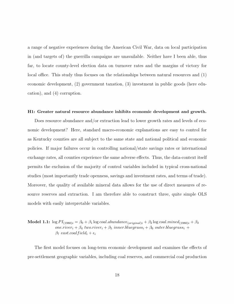
H1: Greater natural resource abundance inhibits economic development and growth.

Does resource abundance and/or extraction lead to lower growth rates and levels of eco-

nomic development? Here, standard macro-economic explanations are easy to control for

as Kentucky counties are all subject to the same state and national political and economic

policies. If major failures occur in controlling national/state savings rates or international

exchange rates, all counties experience the same adverse effects. Thus, the data-context itself

permits the exclusion of the majority of control variables included in typical cross-national

studies (most importantly trade openness, savings and investment rates, and terms of trade).

Moreover, the quality of available mineral data allows for the use of direct measures of re-

source reserves and extraction. I am therefore able to construct three, quite simple OLS

models with easily interpretable variables.

Model 1.1: logPI(1980)i = β0 + β1 log coal.abundance(original)i + β2 log coal.mined(1980)i + β3

one.riveri + β4 two.riveri + β5 inner.bluegrassi + β6 outer.bluegrassi +β7 east.coalfieldi + εi

The first model focuses on long-term economic development and examines the effects of

pre-settlement geographic variables, including coal reserves, and commercial coal production

18

on contemporary income levels. The unique availability of measurements for both the orig-

inal, pre-mining volume of coal in Kentucky and the total coal extracted up until 1980, by

county, provides a unique opportunity to separate resource abundance (understood here as

the mere presence of a resource) from its actual production. No controls for “initial” per

capita income and inequality are included because coal abundance estimates and all other ge-

ographic variables precede the white settlement of Kentucky.39 Initially, just coal abundance

and coal extraction are regressed on 1980 per capita personal income. Then, two dummy

variables are incorporated to account for the effects of riverine networks on development.

Prior to the advent of railroads, navigable rivers were the only way to transport products

that could not walk themselves to market.40 For each county: one.river is coded 1 if at

least one navigable river borders or runs through the county and 0 otherwise; two.river is

similarly coded but for two navigable rivers.41 Then, two additional dummy variables are

incorporated to measure agricultural soil quality as this too is likely to affect both early

urban development as well as long-term growth. The Kentucky Bluegrass region, named

after the lush grass that grows there, sits atop ordovician limestone deposits that generate

particularly good soil for agriculture.42 The inner bluegrass subregion has marginally better

soil quality than the outer bluegrass; but together they comprise the best agricultural land

in the state. Each variable (inner.bluegrass and outer.bluegrass) is coded 1 if a significant

portion of the county lies on that geological zone and 0 otherwise. Finally, a dummy variable

39White settlement in Kentucky began with Daniel Boone’s 1775 expeditionary party. Native Americansettlement patterns are not considered as they were all eventually forced westward after a series of wars withthe British and then the early American states.

40The first major railroad line in Kentucky, connecting Louisville to Nashville, Tennessee was completedin 1859. Yet, Kentucky’s more than 1000 miles of navigable waterways remained the state’s most extensivetransportation network for another decade, until railroad mileage surpassed it in 1870. (Harrison and Klotter,1997, p.135 and p.313).

41There is only one county in all of Kentucky (Livingston) that has access to 3 navigable rivers.42McDowell, 2001.

19

is added for the Eastern Coalfield, which has much poorer soil quality than even the Western

Coalfield (coded 1 if the county lies in the Eastern Coalfield and 0 otherwise).43

Model 1.2: logPI(2005)i = β0 + β1 log coal.abundance(1980)i + β2 log coal.mined(1980−2004)i+β3 logPI(1980)i + β4 poverty(2004)i + εi

The second model examines the effect of coal abundance and production on medium-term

economic development. A measure for coal abundance in 1980 is constructed by subtracting

the volume of coal extracted up until 1980 from the estimates of original county coal en-

dowments. This abundance variable, along with total coal production from 1980-2004,44 are

then regressed on 2005 per capita personal income. Following Sachs and Warner,45 controls

are added for initial income (here, 1980 per capita personal income) and inequality (here, the

percentage of residents living below the poverty line in 2004). 2004 was the only year county

poverty levels were available. The direction of bias, however, can be accounted for and thus

compensated for: poverty levels from one year prior to the dependent variable should predict

average income better than those from several years prior (its estimate will be biased in an

upward direction, potentially reducing the impact of other variables). Controlling for 1980

income levels also controls for the effects of resource abundance and the other geographical

variables prior to that year.

Model 1.3: Growthi = β0+β1 logPI(1980)i+β2 log coal.abundance(1980)i+β3 log coal.mined(1980−2004)i

+β4 poverty(2004)i + εi

43See “A Report on Natural Resources,” in Reports of the Committee for Kentucky, 1943-1950, p.30-32.44Some of the smallest coal producing counties were estimated from geological survey data as they were

lumped together as an “other” category in the original production data. See the appendix for furtherinformation on data sources.

45Sachs, 1995.

20

The third model follows the second in analyzing medium-term development but takes

average growth as the dependent variable, thereby replicating the model used by Sachs

and Warner in their 1995 paper, “Natural Resource Abundance and Economic Growth.” A

standard growth model is utilized for the 1980-2005 period:

1T

log(Y i

T

Y i0

) = δ0 + δ1 log(Y i) + δ′Zi + εi

where growth, measured as the yearly average of the log of income at time T divided by in-

come at time 0, is a negative function of initial income and a vector of growth determinants,

Z.46 Potentially excluded growth determinants include government investment in infrastruc-

ture, as well as county savings and investment rates. It is questionable whether the former

would actually impact local growth as banks operate across counties and low savings rates in

any particular county would probably not decrease the available amount of capital for loans

in that county.

H2: Resource rents lead to lower rates of public taxation.

The claim that natural resource wealth causes less accountable and more authoritarian

governance depends on a logically prior causal claim: that resource rents free governments

from taxing their populations. Without such direct public taxation, it is then argued, citizens

will demand less accountability and democracy from their governments.47 Yet, as previously

discussed, the inclusion of GDP in the measure for resource rents has prevented this claim

from being effectively evaluated.

I believe that Kentucky counties provide an ideal set of cases to test the first part of this

mechanism: that high resource rents will decrease taxation levels. First, the argument can

46Sachs, 1995.47Ross, 2001.

21

certainly be translated into the local setting: we can imagine that access to resource rents

would tempt politicians to increase their popularity by issuing tax cuts or, at the very least,

not raising taxes while still maintaining or expanding county services (fire, police, schools,

etc.). This, in turn, could lead to increasing dependence on resource rents and, hence, the

coal industry, thereby lowering accountability to the general public. Second, each county

has control over its own rate of property taxation (real estate, tangible personal property,

and motor vehicles). The state government of Kentucky, however, sets the taxation rate

on coal mining and then returns 50% of revenues to their county of origin.48 The rate of

resource taxation is thus entirely exogenous to local politics and is, moreover, not itself

causally effected by local tax rates. Thus, results may be clearly interpreted as an effect of

resource rents on local taxes, and not vice versa.

We can thus answer the question, do politicians in counties that receive the “easy money”

generated by resource rents keep public tax rates artificially low? To do so, I construct two

different models. The first model takes as its dependent variable the county property tax

rate (in cents per $100) from 2002-2006, averaged across real estate, tangible personal prop-

erty, and motor vehicles.49 The second model analyzes each county’s tax effort, measured

in 1997 using the standard comparison formulas developed by the Advisory Commission on

Intergovernmental Relations (ACIR).50 This measure essentially weights county tax rates by

type (property, sales, motor vehicle, etc...) according to the relative size of their average

48Some restrictions are placed on what the returned coal money can be spent on. Administrative salaries, inparticular, are excluded. Nonetheless, returned severance taxes can be spent on a wide variety of economicdevelopment projects and social services including roads, law enforcement, health, recreation, libraries,workforce training, and environmental protection, among others. (Kentucky Governor’s Office for LocalDevelopment, Office of State Grants: Program Guide, June 2007 ).

49This model excludes taxes levied in support of the school system, which will be considered separatelyunder the third hypothesis.

50Applied to Kentucky counties by William H. Hoyt of the Center for Business and Economic Research ofthe University of Kentucky, and published in the 2008 Kentucky Annual Economic Report.

22

bases across the state and then applies each county’s individual tax rates to those averages,

thereby creating a comparable measure of how much revenue a county’s tax rates would

generate if all counties had the same tax base. Both models use the same set of independent

and control variables: the log of the average amount of returned severance taxes over the

previous five years,51 the log of the county population (to control for county size), and the

log of average personal income (to control for county wealth). Unemployment is included in

the first model, but not the second, as county-level employment data does not extend back

to 1996. Both population and personal income are lagged by one year as county tax rates

are determined in the year prior to their implementation.

Model 2.1: countyij = β0 + β1 log severence.avrij + β2 log county.pop(i−1)j + β3 logPI(i−1)j+β4 unemploy(i−1)j + εij

Model 2.2: tax.effort1997i = β0 + β1 log severence.avr1991−1996i + β2 log county.pop1996i+β3 logPI1996i + εi

H3: Resource rents lead to lower rates of investment in public goods, especially ineducation.

Research in both economics and political science suggests that the possession of natural

resources can divert government expenditures away from the provision of public goods, espe-

cially education. Employment in the production of natural resources may not require much

education and, if that sector dominates the economy, neither individuals nor governments

51A note of explanation is in order for the treatment of the returned severance taxes, which are predomi-nantly from coal but include other mineral rents as well. Data for these taxes is only currently available forevery other tax year. Thus, in order to create a reliable and consistent indicator, for each year I average thereported returned severance taxes, where available, from the previous five years. Although not perfect, thismeasure should capture the relevant fluctuations experienced by coal counties in their expected incomes fromseverance taxes, which would then theoretically influence their decisions to raise or lower local tax rates.

23

may see much point in devoting time and limited finances to the school system. Also, if

resource rents are used to build patronage networks through the provision of divisible, pri-

vate goods, public education may also suffer.52 Arguably, either of these mechanisms is just

as likely to operate in both local and national contexts, as well as in both democratic and

authoritarian systems.

Do coal-rich Kentucky counties devote fewer resources to public education than their

non-resource endowed counterparts? To answer this question, I construct two time series

models covering the same period (2002-2006) and incorporating the same set of independent

and control variables (the same as in Models 2.1 and 2.2). They differ in that I employ two

different measures for the outcome variable, each of which attempts to capture the concept

of public investment in education. Model 3.1 uses the rate of county school taxes (in cents

per $100 of assessed property value) as its dependent variable. Each county in Kentucky has

its own school district and levy’s a local property tax specifically for school funding. This

measure thus captures the relative effort counties make to raise school funds through prop-

erty taxes, but does not reflect the actual amount of money invested in education. Indeed,

nothing precludes the county from drawing money from other revenue sources, including

resource rents and state coffers, to supplement this funding. Therefore, Model 3.2 takes as

its dependent variable per pupil spending by county. This measure, however, also captures

state funding, which is disproportionately directed toward poorer districts. Each measure

should provide a robustness check against the other.

Model 3.1: school.taxij = β0 + β1 log severence.avrij + β2 log county.pop(i−1)j + β3 logPI(i−1)j

+β4 unemploy(i−1)j + εij

52Although schools do provide what can amount to a substantial proportion of local jobs in rural areas,and thus can themselves become a successful vehicle for political patronage.

24

Model 3.2: stu.expendij = β0 + β1 log severence.avrij + β2 log county.pop(i−1)j + β3 logPI(i−1)j

+β4 unemploy(i−1)j + εij

H4: Natural resource abundance and/or resource rents lead to higher rates ofcorruption.

It is hypothesized that the production of natural resources, and the rents it generates,

create incentives for rent-seeking behavior, patronage, and other forms of corruption. In

Kentucky, resource rents are collected by the state government and returned, in part, to

the counties annually. This difference in context from cross-national studies is critical: the

counties themselves have a diminished capacity to rent-seek as they are neither in charge of

the collection of severance taxes nor the distribution of licenses and contracts for mining.

Nevertheless, they do receive rents from the production and sale of coal. We can thus

examine whether merely increasing the pot of non-tax based revenues in turn increases the

likelihood of corruption.

To evaluate this hypothesis, I first construct a dichotomous corruption variable. Corrup-

tion is notoriously difficult to measure. It often simply goes unreported. And even when

caught, its duration and true extent might remain uncertain. It thus makes little sense to

construct a yearly variable or to try and use dollar figures to estimate a continuous variable

as any such measure would end up extremely noisy and unreliable. Instead, I examined the

yearly financial audits for the County Clerk’s offices and the County Fiscal Courts between

2000 and 2006. In Kentucky, these are the only two government offices at the county level

that have direct access to resource rents. If there was an instance of corruption detected in

a county at any point during this time period, the corruption variable was coded as 1. If all

of the audit reports were clean, the variable was coded as 0.

But what counts as corruption? This is another notoriously difficult question to answer.

25

For the sake of this study, I used the following coding guidelines: If an instance of financial

misconduct in an audit was referred to the Kentucky or U.S. Attorney General’s Office, Law

Enforcement, the Kentucky Department of Revenue, and/or the IRS for criminal reasons,

the county was automatically coded a 1. If an instance of egregious financial misconduct

was for some unknown reason not referred to such agencies, then the county was still coded

as a 1 if the infringement contained one or more of the following practices: illegal use of

private contractors, extremely questionable and unaccounted for expenditures on roadwork

or construction projects, or the violation of the ethics code in the distribution of government

contracts (such as giving them to family members without a competitive bidding process).

In all other cases, the county received a 0 coding, even if they were cited for some violation

of state accounting and financial management codes.

Using this dichotomous dependent variable for corruption, I then created two probit

models: Model 4.1 is a simple comparison between the corruption variable and a dichoto-

mous variable indicating whether or not a county produced coal. This model is intended to

demonstrate, at an incredibly simplified level, whether or not there is any reason to think

that natural resources and government corruption are linked in Kentucky. Model 4.2 is a

more sophisticated analysis of the effect of coal abundance and resource rents on county

corruption which includes controls for the size (population), wealth (per capita personal in-

come), and poverty rate of the county.

Model 4.1: corruptioni = β0 + β1coali + εi

Model 4.2: corruptioni = β0 + β1 log abundance(1980)i + β2 log severence(1999−2005)i+

β3 logPI.avr(2001−2005)i + β4 log county.pop(2004)i + β5poverty(2004)i + εi

26

7 Results

Generally, the findings of this paper both support and raise challenges for the paradox

of the resource curse. There is some evidence that natural resource abundance does indeed

inhibit long-term growth, albeit through more indirect mechanisms that typically proposed.

On the political side, however, their is no evidence that natural resources or their associated

rents lead to lower taxation, less investment in public education, or greater corruption.

H1: Greater economic resource abundance inhibits economic development/ growth.

Collectively, the economic development models suggest that if resource abundance does

indeed dampen long term growth rates, it is not through the extraction of the resources

themselves. Indeed, Model 1.1 finds a positive and significant correlation between coal pro-

duction and county incomes (although the magnitude of the effect is quite small). In models

1.2 and 1.3, neither coal abundance nor mining activity seem to have any effect on medium-

term growth. The only other statistically significant resource variable is the indicator for the

Eastern Coalfield. Location in this subregion of the state, all else being equal, is correlated

with a 22% decline in long-term economic growth. But is this due to the presence of coal?

Remember that the Eastern Coalfield has remarkably poor soil quality—far worse than even

the Western Coalfield. Combined with the observed effects of being located in either the

inner or outer bluegrass subregions (respectively a 31% and 10% increase in observed in-

come levels), this suggests that the underlying causal story may be rooted in geology. It

is probably not a coincidence that, in Kentucky, the bluegrass counties were the first to be

settled, have historically led agricultural production, and also became the locus of many

of Kentucky’s urban areas. Indeed, it is quite remarkable that this small set of variables,

focused on geological and geographical characteristics of the land, actually explains roughly

27

34% of modern income distribution across counties (removing the coal production variable

reduces the R2 by about two percentage points).

Model 1.1logPI(1980)i = β0 + β1 log coal.abundance(original)i + β2 log coal.mined(1980)i + β3one.riveri+

β4 two.riveri + +β5 inner.bluegrassi + β6 outer.bluegrassi + β7 east.coalfieldi + εi

a b cVariable Coefficient Coefficient Coefficient

(SE) (SE) (SE)

constant 8.8727*** 8.7901*** 8.7357***(0.0254) (0.0318) (0.0374)

log original coal abundance -0.0098 -0.0102 -0.0029(0.0069) (0.0065) (0.0059)

log coal mined through 1980 0.0068 0.0081 0.0126*(0.0080) (0.0076) (0.0068)

one navigable river 0.1224*** 0.0845**(0.0375) (0.0339)

two navigable rivers 0.1402* 0.1608**(0.0747) (0.0680)

inner bluegrass 0.3094***(0.0740)

outer bluegrass 0.0970**(0.0447)

eastern coalfield -0.2222***(0.0538)

Adusted R2 0.0283 0.1456 0.3357

Model 1.1.a: Breusch-Pagan Test: χ2 = 3.9868, p = 0.0459

Model 1.1.b: Breusch-Pagan Test: χ2 = 0.0091, p = 0.9240

Model 1.1.c: Breusch-Pagan Test: χ2 = 2.2793, p = 0.0000

Computing HAC robust errors neither diminished the magnitude nor the significance of the results.

The more conservative, original estimates are thus reported.

∗ ∗ ∗ = p ≤ 0.001, ∗∗ = p ≤ 0.01, ∗ = p ≤ 0.05

28

Models 1.2 and 1.31.2: logPI(2005)i = β0 + β1 log coal.abundance(1980)i + β2 log coal.mined(1980−2004)i + β3 logPI(1980)i

+β4 poverty(2004)i + εi

1.3: Growthi = β0 + β1 logPI(1980)i + β2 log coal.abundance(1980)i + β3 log coal.mined(1980−2004)i

+β4poverty(2004)i + εi

1.2 1.3Personal Income Growth

a b a bVariable Coefficient Coefficient Coefficient Coefficient

(SE) (SE) (SE) (SE)

constant 4.0640*** 5.7328*** 0.1563*** 0.2205***(0.4872) (0.6806) (0.0187) (0.0262)

1980 personal 0.6832*** 0.5134*** -0.0122*** -0.0187***income (0.0549) (0.0728) (0.0021) (0.0028)1980 coal -0.00004 0.0006 -0.0000 0.0000abundance (0.0042) (0.0040) (0.0002) (0.0002)coal mined -0.0053 -0.0022 -0.0002 -0.00011980-2004 (0.0048) (0.0047) (0.0002) (0.0002)2004 poverty -0.0107*** -0.0004***rate (0.0032) (0.0001)

Adjusted R2 0.6143 0.6459 0.26 0.3206

Model 1.2.a Breusch-Pagan Test: χ2 = 0.0004, p = 0.9834

Model 1.2.b Breusch-Pagan Test: χ2 = 0.0028, p = 0.9581

Model 1.3.a Breusch-Pagan Test: χ2 = 1.3801, p = 0.2401

Model 1.3.b Breusch-Pagan Test: χ2 = 2.1091, p = 0.1464

∗ ∗ ∗ = p ≤ 0.001, ∗∗ = p ≤ 0.01, ∗ = p ≤ 0.05

Mining activity, in the absence of agricultural possibilities, may also be ill-suited to long-

term, sustained growth. While resource extraction certainly generates income while the

mines are open, individual mines do eventually close. When the mineral or fuel resources on

a particular piece of land are exhausted, the resource business moves on to greener pastures,

withdrawing all of the indirect as well as direct benefits they bring to the local economy.

Jobs, people, and money may all rapidly depart. Where no alternative industries also support

29

the economy (such as agriculture), you would get a veritable “ghost town” effect that would

surely set back local development and growth for some time.53 Multiplying this effect across

many locales may also have significant repercussions for larger economic units, such as states

and countries.

Alternatively, the seemingly contradictory results between the models (that long-term

growth in the eastern coalfield is depressed while coal seems to have no effect on medium-

term growth) may be a remnant of the traumatic experience of mining mechanization. In the

beginning of the 20th century, coal production expanded rapidly in the Eastern Coalfield,

leading to the large-scale migration of workers and their families to the region. By 1940,

the coal workforce in eastern Kentucky had expanded to around 63,000 laborers. Then,

in the following decade and a half, mechanization led mining employment to fall by some

70%. Many people simply left, looking for work elsewhere. The net population loss (around

25,000), however, still could not compensate for the volume of jobs lost and unemployment

soared.54 Nonetheless, the shock of rapid mechanization was experienced across the coal

industry, in both the Eastern and Western Coalfields. and yet the Eastern Coalfield counties

have experienced significantly slower growth.55

53Moreover, extractive industries often leave the land environmentally damaged and unsuitable for anytype of post-mining use. Currently, the national Abandoned Mine Land Inventory System (AMLIS), countsroughly 40,000 acres of high priority (levels 1 and 2) damaged land in Kentucky; hazards that include cloggedstreams, landslide prone hillsides, polluted water, underground fires, and vertical shafts, among other suchdangers to humans and wildlife. Such land requires major reclamation efforts before it can be converted toother uses, even to state and national parks.

54Harrison and Klotter, 1997, p.310 and p.367; Eastern Kentucky Regional Planning Commission Program60, 1960-1970, p.IV.

55If a separate indicator variable for the Western Coalfield is included in the regression the differencebetween their coefficients is 0.1858. In other words, the growth rate of the East was depressed by roughlyan additional 19%.

30

H2: Resource rents lead to lower rates of public taxation.

The statistical evidence does not support the hypothesis that Kentucky counties bene-

fiting from coal rents tax their publics any less than other counties. In fact, in Model 2.1,

resource rich counties tax property at higher average rates, a statistically significant finding.

The magnitude of the effect, however, is minimal: a 1% increase in returned coal rents is

associated with an increase of 1-2 cents per $1000 of assessed property value (which would

Models 2.1 and 2.22.1 DV= County Property Tax Rate (cents per $100)

countyij = β0 + β1 log severence.avrij + β2 log county.pop(i−1)j + β3 logPI(i−1)j + β4unemploy(i−1)j + εij

2.2 DV= 1997 Tax Effort

tax.effort1997i = β0 + β1 log severence.avr1991−1996i + β2 log county.pop1996i + β3 logPI1996i + εi

2.1 2.2County Taxes Tax Effort

a bVariable Coefficient Coefficient Coefficient

(PCSE) (PCSE) (SE)

constant 95.3466*** 64.9558*** 421.152(12.8482) (15.8317) (275.867)

severence taxes 0.2931*** 0.1042* 2.002(0.0553) (0.0426) (2.365)

population -6.0579*** -5.4370*** 19.429(0.3585) (0.3328) (18.060)

personal income -10.1960*** -5.0942 -97.378(3.2172) (3.5706) (73.501)

unemployment 0.9160***(0.2205)

Adjusted R2 0.28 0.1625 0.0127

a: N=598, Groups=120, Missing Obs=2 N=120

b: N=598, Groups=120, Missing Obs=2

Breusch-Pagan Test: Breusch-Pagan Test:

a: χ2 = 27.624, p = 0.0000 χ2 = 30.0377, p = 0.0000

b: χ2 = 36.5866, p = 0.0000

∗ ∗ ∗ = p ≤ 0.001, ∗∗ = p ≤ 0.01, ∗ = p ≤ 0.05

31

total no more than a few dollars a year for most homeowners). Nevertheless, this finding

presents a bit of a puzzle: why would counties benefitting from returned coal rents choose

higher rates of taxation? The most likely answer is that coal counties happen to be poorer

on average than other counties, which logically means that their tax base is lower. They

therefore must employ higher tax rates in order to garner the same amount of revenue. In-

deed, there appears to be no effect, in either direction, of resource rents on tax effort, an

arguably better measure that takes into account the extent of each county’s tax base.

H3: Resource rents lead to lower rates of investment in public goods, especiallyeducation.

Neither is their any statistical evidence to support the claim that coal rich counties invest

fewer resources in public education. Returned severance taxes are positively correlated with

both county school taxes (when unemployment is controlled for) and per pupil spending. It is

important to note, however, that the comparison here is largely between resource abundant

rural counties and their agricultural and forested counterparts. Many incorporated urban

areas have their own, independent school districts, funded by special city taxes.56 Residents

in such cities are consequently exempted from paying the county school tax (but not other

county taxes). As the control variables do not distinguish between urban and rural school

districts within a county, city schools had to be excluded from data. Thus, while coal

counties may levy higher taxes or spend more money per pupil than other rural counties,

they may very well tax and spend less than cities. A simple comparison of average school

taxes suggests that this is the case:

56Though by no means do all or even most incorporated cities have independent school districts. In fact,the largest city in the state, Louisville, has been part of the Jefferson County School District since the 1970swhen a federal court ruling forced their merger in order to further integration.

32

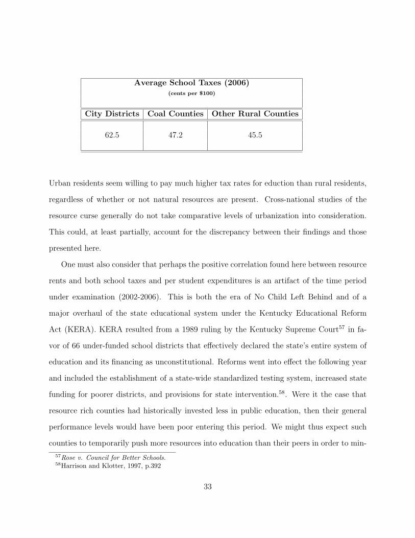
Average School Taxes (2006)(cents per $100)

City Districts Coal Counties Other Rural Counties

62.5 47.2 45.5

Urban residents seem willing to pay much higher tax rates for eduction than rural residents,

regardless of whether or not natural resources are present. Cross-national studies of the

resource curse generally do not take comparative levels of urbanization into consideration.

This could, at least partially, account for the discrepancy between their findings and those

presented here.

One must also consider that perhaps the positive correlation found here between resource

rents and both school taxes and per student expenditures is an artifact of the time period

under examination (2002-2006). This is both the era of No Child Left Behind and of a

major overhaul of the state educational system under the Kentucky Educational Reform

Act (KERA). KERA resulted from a 1989 ruling by the Kentucky Supreme Court57 in fa-

vor of 66 under-funded school districts that effectively declared the state’s entire system of

education and its financing as unconstitutional. Reforms went into effect the following year

and included the establishment of a state-wide standardized testing system, increased state

funding for poorer districts, and provisions for state intervention.58. Were it the case that

resource rich counties had historically invested less in public education, then their general

performance levels would have been poor entering this period. We might thus expect such

counties to temporarily push more resources into education than their peers in order to min-

57Rose v. Council for Better Schools.58Harrison and Klotter, 1997, p.392

33

imally meet new, stricter state and federal laws. This, of course, is purely speculative and a

longer historical time frame merits analysis.

Models 3.1 and 3.23.1 DV= County Schools Tax Rate (cents per $100)

school.taxij = β0 + β1 log severence.avrij + β2 log county.pop(i−1)j + β3 logPI(i−1)j + β4unemploy(i−1)j + εij

3.2 DV= Per Student County Education Expenditures

stu.expendij = β0 + β1 log severence.avrij + β2 log county.pop(i−1)j + β3 logPI(i−1)j + β4unemploy(i−1)j + εij

3.1 3.2School Taxes Per Student Expenditures

a b a bVariable Coefficient Coefficient Coefficient Coefficient

(PCSE) (PCSE) (PCSE) (PCSE)

constant -52.0007*** -14.6930 3.8182*** 3.1362***(3.2283) (9.2163) (0.4416) (0.5504)

severence -3.2283** 0.1678** 0.0091*** 0.0049***taxes (0.0385) (0.0615) (0.0013) (0.0012)population 4.1983*** 3.4361*** -0.0368* -0.0229

(0.1191) (0.2439) (0.0145) (0.0117)personal 18.5284*** 12.2654*** 0.0465 0.1610income (0.8060) (1.6355) (0.1153) (0.1312)unemployment -1.1245*** 0.0205***

(0.2916) (0.0051)

Adjusted R2 0.2029 0.2514 0.0962 0.1899

a: N=598, Groups=120, Missing Obs=2 a: N=596, Groups=120, Missing Obs=4

b: N=598, Groups=120, Missing Obs=2 b: N=596, Groups=120, Missing Obs=4

Breusch-Pagan Test: Breusch-Pagan Test:

a: χ2 = 0.0003, p = 0.9864 a: χ2 = 0.8375, p = 0.3601

b: χ2 = 0.0298, p = 0.8630 b: χ2 = 0.4231, p = 0.5154

∗ ∗ ∗ = p ≤ 0.001, ∗∗ = p ≤ 0.01, ∗ = p ≤ 0.05

34

H4: Natural resource abundance and/or resource rents lead to higher rates ofcorruption.

Historical evidence suggests that both financial and political corruption have long been

prevalent across Kentucky. In the early 20th century, urban and rural political bosses shame-

lessly controlled and sold votes to politicians. In 1909 it was estimated that as many as one

quarter of votes in the average county could be purchased.59 As late as the 1960s, county

jobs were still considered the principal payout to faithful members of the wining political

party.60 While no systematic data exists, historical accounts do not point to a systematic

relationship between natural resources and corruption: political bosses were especially pow-

erful in urban areas, and the political parties seemingly operated their patronage machines

across all counties, regardless of economic base.

Today, corruption is still fairly widespread in Kentucky: nearly one quarter of counties

were coded as having experienced at least one instance of corruption over the short time

period under analysis (25 of 120 counties). The findings from models 4.1 and 4.2, however,

suggest that natural resources are not the cause of this corruption. There is no significant

Model 4.1:corruptioni = β0 + β1coali + εi

DV= instance of corruption coded 1, otherwise 0

Variable Coefficient Standard Error

constant -0.9872*** 0.1822coal county 0.3721 0.2606

Probit Model with dichotomous DV

N=120, Null Deviance= 122.82, Residual Deviance= 120.77

∗ ∗ ∗ = p ≤ 0.001, ∗∗ = p ≤ 0.01, ∗ = p ≤ 0.05

59Harrison and Lowell, 1997, p.251 and 276.60The Southern Appalachian Region: A Survey, 1962, p.154-155.

35

Model 4.2:corruptioni = β0 + β1 log abundance(1980)i+

β2 log severence(1999−2005)i + β3 logPI.avr(2001−2005)i

+β4 log county.pop(2004)i + β5poverty(2004)i + εi

DV= instance of corruption coded 1, otherwise 0

Variable Coefficient Standard Error

constant -1.7623 2.0766

1980 coal -0.1832 0.2688abundanceseverance 0.0203 0.1365taxespopulation 0.6470 2.4383

personal -0.8043 2.4308incomepoverty 0.0922** 0.0319

Probit Model with dichotomous DV

N=120, Null Deviance= 122.82, Residual Deviance= 109.29

∗ ∗ ∗ = p ≤ 0.001, ∗∗ = p ≤ 0.01, ∗ = p ≤ 0.05

relationship between either coal abundance or rents and the dependent variable. Only

poverty has a statistically significant impact on corruption: a 1 percentage point climb

in the poverty rate leads to a 9% increase in the likelihood of corruption. Even when poverty

is removed from the model, the natural resource variables remain insignificant. We can

thus only claim that natural resource wealth, here, affects corruption only insofar as we can

demonstrate that it causes poverty. Merely increasing the pot of non-citizen-based tax rev-

enue does not, in and of itself, lead to increased corruption. If natural resource endowments

do directly cause corruption at other levels of government, then other mechanisms must be

at play, such as control over the distribution of extraction contracts or a state monopoly over

prices. Yet, there is no solid theoretical reason to think that these mechanisms are exclusive

36

to natural resource management. As Bates has argued in the African context, government

control over pricing and contracts pertain to agricultural commodities (through marketing

boards) as well as to many small-scale industries.61

There is, however, a story about corruption and poverty here. Within the county audit

reports, a significant number of counties were repeatedly cited for not complying with state

standards relating to the division of financial duties. Distributing duties across staff members

creates a system of checks and balances for the management of money, making it more

difficult for individuals to steal public funds. In other words, the absence of segregated

financial duties leaves a county particularly vulnerable to corruption. Along with these

citations often came the following note of explanation: that the county in question could not

comply with the state standards because they lacked the financial resources to hire enough

staff. Thus the poorest counties with the fewest resources are the least able to hire sufficiently

large staffs, and are thereby the most vulnerable to corruption. The notion of a threshold

(i.e. n staff members is sufficient to ensure proper segregation of duties) would explain why

poverty rates are significant and income levels are not: it is only the very poorest counties

that cannot afford to buffer themselves against corruption.

8 Conclusions

This paper has attempted to submit four aspects of the resource curse theory to empir-

ical testing, using reliable and easily interpretable measures of abundance and production.

The wealth and growth models suggest that coal counties have indeed developed more slowly

than others. Yet, there is evidence that this effect has little to do with typical macroeconomic

61Bates, 1981, Markets and States in Tropical Africa.

37

explanations and more to do with the underlying geology of the land and its unsuitability

for agriculture. Natural resource production, and mining in particular, may move location

too frequently to support the growth of a stable, secondary local economy. Ghost towns do

not engender development. Neither do significant decreases in labor demand, which may be

caused either by the exhaustion of the resource or by massive upheavals such as the mecha-

nization of an industry. In the political realm, this paper has found no evidence to support

the claim that natural resource abundance and its associated rents lead to lower tax rates,

less investment in public goods, or greater corruption. Rather than using resource rents

as a substitute for public taxation, Kentucky coal counties actually levy property taxes at

higher rates than their non-resource rich counterparts. Severance taxes are also positively

correlated with increased spending on education. Finally, their is no evidence that resource

rents make coal counties more vulnerable to corruption. Only insofar as natural resource

abundance contributes to poverty, does it increase the likelihood of corruption.

While these results are embedded in a particular local context, and must be generalized

with caution, they should still give us pause for they do not support existing hypotheses

connecting natural resource wealth to poor economic and political development. Rather,

this paper points to the importance of understanding how the geological features of the

land may interact with production processes to hinder sustained growth. And if poverty is

the conduit through which natural resources hurt political development, then solving the

problem of resources and slow growth would also have far-reaching secondary benefits in the

political sphere.

38

9 Appendix: Data Sources

(1) Coal Abundance and Severance Taxes:

Provided by the Kentucky Governor’s Office of Energy Policy, the Division of Fossil Fuels &Utility Services. Coal abundance figures are contained in the Blue Book of Kentucky Coaland Severance Tax numbers are published in the biannual Kentucky Coal Facts Guide. Bothwere generously provided by Dennis McCully, the Western Kentucky Coal Representative.Missing 2005 cumulative production data for the smallest producer counties was estimatedfrom the Kentucky Geological Survey (online: http://www.uky.edu/KGS/coal/production/kycoal01.htm [last accessed July 31, 2009]).

(2) Corruption:

Data collected from annual audit reports of Kentucky County Clerk’s Offices and FiscalCourts. Reports are available from the Office of the Kentucky Auditor of Public Accounts(online by county: http://www.auditor.ky.gov/Public/Audit Reports/ KentuckymapSearch.asp[last accessed March 28, 2008]).

(3) County Property and School Taxes:

Available from the Kentucky Department of Revenue’s annual tax books (online: http://revenue.ky.gov/newsroom/publications.htm#PTR [last accessed July 31, 2008]).

(4) Educational Expenditures:

Data on per student spending by county as well as on student achievement and standardizedtest scores is publicly available from the Kentucky Department of Education’s School ReportCard Archive (online by county: http://apps.kde.state.ky.us/schoolReportCardArchive/ [lastaccessed March 28, 2008]).

(5) Navigable Rivers and Bluegrass Counties:

Obtained by compiling information from the following maps and accompanying documents:(a) map of navigable Kentucky rivers (online: www.waterwayscouncil.org [last accessedSeptember 14, 2008]); (b) map of Kentucky rivers overlaid on Kentucky counties (online:http://geology.com/state-map/kentucky.shtml [last accessed September 14, 2008]); (c) gen-eralized geological map of Kentucky (online: http://www.uky.edu/ KentuckyAtlas/map-kentucky-geologic.gif [last accessed September 15, 2008]); (d) the pamphlet “The Geology of

39

Kentucky: A Text to Accompany the Geologic Map of Kentucky” from the US GeologicalSurvey of the US Department of the Interior (online: http://pubs.usgs.gov/pp/p1151h/index.html [last accessed September 15, 2008]).

(6) Personal Income and Population:

Data is available for the years 1999-2005 from the Regional Economic Information Systemof the Bureau of Economic Analysis, housed in the U.S. Department of Commerce (online:http://www.bea.gov/regional/reis/ca1-3fn.cfm [last accessed January 10, 2008]).

(7) Poverty Rates and Unemployment:

Available from the U.S. Census Bureau, Data Integration Division, Small Area EstimatesBranch (online: http://www.census.gov/hhes/www/saipe/index.html [last accessed January10, 2008]).

40

References

[1] A report on natural resources. In Reports of the Committee for Kentucky, 1943-1950.Committee for Kentucky, 1950.

[2] The Southern Appalachian Region: A Survey. University of Kentucky Press, 1962.

[3] Eastern Kentucky Regional Planning Commission Program 60, 1960-1970. EasternKentucky Regional Plannign Commission, 1970.

[4] James E. Alt and David Dreyer Lassen. The political economy of institutions andcorruption in american states. Journal of Theoretical Politics, 15(3):341–365, 2003.

[5] R. M. Auty, editor. Resource Abundance and Economic Development. Oxford UniversityPress, 2001.

[6] R. E. Baldwin. Economic Development and Export Growth: A Study of Northern Rhode-sia, 1920-1960. University of California Press, 1966.

[7] Robert H. Bates. Markets and States in Tropical Africa: The Political Basis of Agri-cultural Policies. University of California Press, 1981.

[8] Hazem Beblawi and Giacomo Luciani, editors. The Rentier State. Croom helm and theIstituto Affari Internazionali, 1987.

[9] Paul Collier and Anke Hoeffler. On economic causes of civil war. Oxford EconomicPapers, 50:563–573, 1998.

[10] John T. Cuddington. Long run trends in 26 primary commodity prices. Journal ofDevelopment Economics, 39, October 1992.

[11] Vaughn M. Elliott, Valentina Hartarska, and Conner Bailey. Stunted growth: Naturalresource concentration, economic growth, and dutch disease in the southeastern unitedstates. Southern Agricultural Economics Association Annual Meetings in Dallas, Fen-ruary 3-6, 2008.

[12] Pierre Englebert and James Ron. Primary commodities and war: Congo-brazzaville’sambivalent resource curse. Comparative Politics, 37(1):61–81, October 2004.

[13] Kentucky Governor’s Office for Local Development. Office of state grants: Programguide, June 2007.

[14] Alan Gelb, editor. Oil Windfalls: Blessing or Curse? World Bank Research Publication,1988.

41

[15] Ellis Goldberg, Erik Wibbels, and Eric Mvukiyehe. Lessons from strange cases: Democ-racy, development, and the resource curse in the u.s. states. Comparative PoliticalStudies, 41(4/5):477–514, 2008.

[16] Thorvaldur Gylfason. Natural resources, education, and economic development. Euro-pean Economic Review, (45):847–859, 2001.

[17] Lowell H. Harrison and James C. Klotter. A New History of Kentucky. The UniversityPress of Kentucky, 1997.

[18] Albert O. Hirschman. The Strategy of Economic Development. Yale University Press,1958.

[19] William H. Hoyt. Variations in Tax Effort and Tax Bases among Kentucky Counties.Center for Business and Economic Research, University of Kentucky, 2000.

[20] Macartan Humphreys. Natural resources, conflict, and conflict resolution. Journal ofConflict Resolution, 49(4):508–537, 2005.

[21] Smail Khennas, editor. Industrialization, Mineral Resources and Energy in Africa.CODESRIA, 1993.

[22] Younkyoo Kim. The Resource Curse in a Post-Communist Regime: Russia in Compar-ative Perspective. Aldershot, 2003.

[23] P. Lane and A. Tornell. Power concentration and growth. Harvard Institute of EconomicResearch Discussion Paper, (1720), 1995.

[24] Carlos Leite and Jens Weidmann. Does mother nature corrupt? natural resources,corruption, and economic growth. Working Paper of the International Monetary Fund,1999.

[25] Robert C. McDowell. The geology of kentucky: A text to accompany the geologicalmap of kentucky. Technical report, U.S. Geological Survey, 2001.

[26] Kentucky Office of Energy Policy and the Kentucky Coal Association. Kentucky coalfacts: 2005-2006 guide, 2006.

[27] Office of Surface Mining: Reclamation and Enforcement. Abandoned mine land inven-tory system (amlis).

[28] Gwenn Okruhlik. Rentier wealth, unruly law, and the rise of opposition: The politicaleconomy of oil states. Comparative Politics, 31(3):295–315, April 1999.

42

[29] Michael L. Ross. The political economy of the resource curse. World Politics, 51(2):297–322, 1999.

[30] Michael L. Ross. Does oil hinder democracy? World Politics, 53:325–61, April 2001.

[31] Michael L. Ross. What do we know about natural resources and civil war? Journal ofPeace Research, 41(3):337–356, May 2004.

[32] Jeffrey D. Sachs and Andrew M. Warner. Natural resource abundance and economicgrowth. Harvard Institute for International Development Discussion Paper, (517a),October 1995.

[33] Jeffrey D. Sachs and Andrew M. Warner. The big push, natural resource booms andgrowth. Journal of Development Economics, 59:43–76, 1999.

[34] Jeffrey D. Sachs and Andrew M. Warner. Natural resources and economic development:The curse of natural resources. European Economic Review, (45):827–838, 2001.

[35] A. Schleifer and R. Vishney. Corruption. Quarterly Journal of Economics, 59:599–617,1993.

[36] D. Seers. The mechanism of an open petroleum economy. Social and Economic Studies,13:233–242, 1964.

[37] Benjamin Smith. Oil wealth and regime survival in the developing world, 1960-1999.American Journal of Political Science, 48(2):232–246, 2004.

[38] Dirk Vandewalle. Libya since Independence: Oil and State-Building. Cornell UniversityPress, 1998.

[39] Douglass A. Yates. The Rentier State in Africa: Oil Rent Dependency and Neo-Colonialism in the Republic of Gabon. Africa World Press, 1996.

43