ES 240: Scientific and Engineering Computation....

ES 240: Scientific and Engineering Computation. Interpolation

PolynomialPolynomial

Definition– a function f(x) that can be written as a finite series of power functions

like

– fn is a polynomial of order n– A polynomial is represented by coefficient vector from highest power.– p1=[3 -5 -7 1 9] p1(x) = 3x4 - 5x3 – 7x2 + x + 9

in

iin xaxf ∑

=

=0

)(


Polynomial OperationsPolynomial Operations

poly(r)– convert roots to a polynomial– r=[ 1 2 3 ]; poly(r)

roots(p)– find roots of a polynomial– p=[ 2 3 4 ]– roots(p)

Y = polyval(p, x)– returns the value of a polynomial, p(x). – P is a vector of length N+1 whose elements are the coefficients of the

polynomial in descending powers.– p=[3 -5 -7 1 9] p(x) = 3x4 - 5x3 – 7x2 + x + 9



P = polyfit(x, y, n)– Returns the least squares fit coefficients of a polynomial

p(x) of degree n– P is of length N+1.

conv(p1,p2)– multiply two polynomials p1 and p2– conv(p1,p2)[q r]=deconv(p1,p2)– polynomials p1 divide by p2, where q is quotient and r is

remainder– [q r]=deconv(p1,p2)



polyint(p,c)– integrate of polynomial p with integration constant c

(default 0)– polyint(p)– polyint(p,1)

polyder(p)– differentiate polynomial p respective to x– >> polyder(p)


Curve FittingCurve Fitting

Applications– Estimating the value of points between discrete values– Simplifying complicated functions

Methods– Interpolation

• Data are very precise • curve passes through all points

– curve fitting• Data are just approximations• curve represent a general trend of the data


Curve Fitting and InterpolationCurve Fitting and Interpolation

Curve Fitting(linear or non-linear)

Linear Interpolation(most popular interpolation)

Other Interpolation(higher order polynomial,

spline, nearest,…)


Linear InterpolationLinear Interpolation

The linear interpolation is achieved by fitting a line between two known data points

The resulting formula based on known points x1 and x2 and the values of the dependent function at those points is:

f1 x( )= f x1( )+f x2( )− f x1( )

x2 − x1

x − x1( )


Quadratic (Polynomial) InterpolationQuadratic (Polynomial) Interpolation

One problem that can occur with solving for the coefficients of a polynomial is that the system to be inverted is in the form:

Matrices such as that on the left are known as Vandermonde matrices, and they are very ill-conditioned - meaning their solutions are very sensitive to round-off errors.The issue can be minimized by scaling and shifting the data.

x1n−1 x1

n−2 L x1 1x2

n−1 x2n−2 L x2 1

M M O M Mxn−1

n−1 xn−1n−2 L xn−1 1

xnn−1 xn

n−2 L xn 1

⎡

⎣

⎢ ⎢ ⎢ ⎢ ⎢

⎤

⎦

⎥ ⎥ ⎥ ⎥ ⎥

p1p2M

pn−1pn

⎧

⎨ ⎪ ⎪

⎩ ⎪ ⎪

⎫

⎬ ⎪ ⎪

⎭ ⎪ ⎪

=

f x1( )f x2( )

Mf xn−1( )f xn( )

⎧

⎨

⎪ ⎪

⎩

⎪ ⎪

⎫

⎬

⎪ ⎪

⎭

⎪ ⎪


Newton Interpolating PolynomialsNewton Interpolating Polynomials

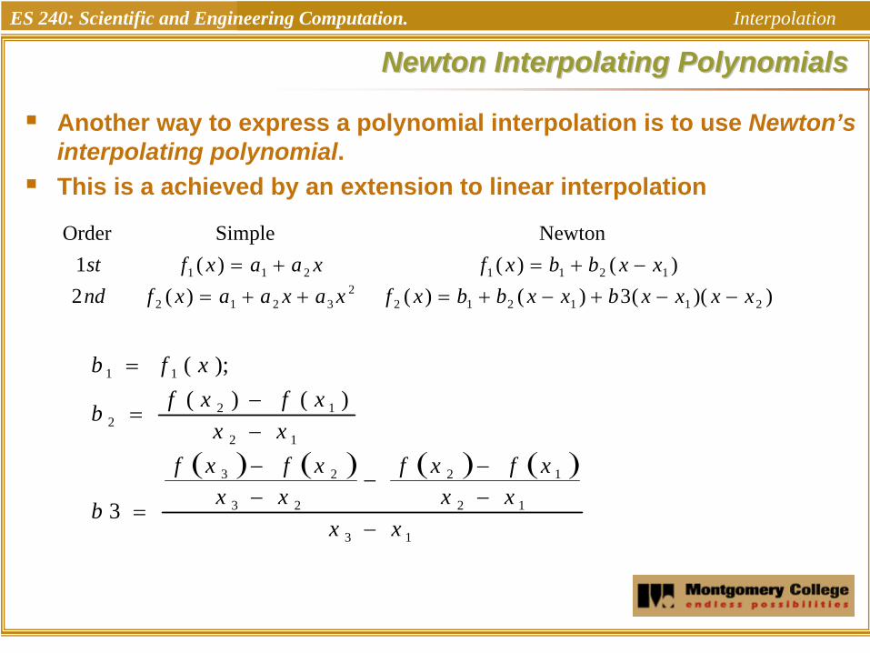
Another way to express a polynomial interpolation is to use Newton’s interpolating polynomial.This is a achieved by an extension to linear interpolation

))((3)()()(2)()()(1

NewtonSimpleOrder

2112122

3212

1211211

xxxxbxxbbxfxaxaaxfndxxbbxfxaaxfst

−−+−+=++=−+=+=

( ) ( ) ( ) ( )

13

12

12

23

23

12

122

11

3

)()();(

xxxx

xfxfxx

xfxf

b

xxxfxfb

xfb

−−−

−−−

=

−−

=

=


Newton Interpolating Polynomials (cont)Newton Interpolating Polynomials (cont)

The second-order Newton interpolating polynomial introduces some curvature to the line connecting the points, but still goes through the first two points.

The resulting formula based on known points x1, x2, and x3 and the values of the dependent function at those points is:

( ) ( ) ( ) ( ) ( )( ) ( ) ( ) ( )

( )( )2113

12

12

23

23

112

1212 xxxx

xxxx

xfxfxx

xfxf

xxxx

xfxfxfxf −−−

−−

−−−

+−−−

+=


GeneralizationGeneralizationAn (n-1)th Newton interpolating polynomial has all the terms of the (n-2)th polynomial plus one extra.

The general formula is:where

and the f[…] represent divided differences.

fn−1 x( )= b1 + b2 x − x1( )+L+ bn x − x1( ) x − x2( )L x − xn−1( )

b1 = f x1( )b2 = f x2, x1[ ]b3 = f x3, x2, x1[ ]M

bn = f xn, xn−1,L, x2 , x1[ ]


Divided DifferencesDivided Differences

Divided difference are calculated as follows:

Divided differences are calculated using divided difference of a smaller number of terms:

f xi , x j[ ]=f xi( )− f x j( )

xi − xj

f xi , x j , xk[ ]=f xi , xj[ ]− f x j , xk[ ]

xi − xk

f xn, xn−1,L, x2, x1[ ]=f xn, xn−1,L, x2[ ]− f xn−1, xn−2,L, x1[ ]

xn − x1


ExampleExample

15.115.1

Do by handDo by hand

Use the Use the newtintnewtint functionfunction


Lagrange Interpolating PolynomialsLagrange Interpolating Polynomials

Weighted average of the two values being connectedThe differences between a simple polynomial and Lagrange interpolating polynomials for first and second order polynomials is:

where the Li are weighting coefficients that are functions of x.

Order Simple Lagrange1st f1(x) = a1 + a2x f1(x) = L1 f x1( )+ L2 f x2( )2nd f2 (x) = a1 + a2x + a3x

2 f2 (x) = L1 f x1( )+ L2 f x2( )+ L3 f x3( )


Lagrange Interpolating Polynomials (cont)Lagrange Interpolating Polynomials (cont)

The first-order Lagrange interpolating polynomial may be obtained from a weighted combination of two linear interpolations, as shown.

The resulting formula based on known points x1 and x2 and the values of the dependent function at those points is:

f1(x) = L1 f x1( )+ L2 f x2( )

L1 =x − x2

x1 − x2

, L2 =x − x1

x2 − x1

f1(x) =x − x2

x1 − x2

f x1( )+x − x1

x2 − x1

f x2( )


Lagrange Interpolating Polynomials (cont)Lagrange Interpolating Polynomials (cont)

In general, the Lagrange polynomial interpolation for n points is:

where Li is given by:

fn−1 xi( )= Li x( ) f xi( )i=1

n

∑

Li x( )=x − xj

xi − x jj=1j≠i

n

∏


ExampleExample

15.115.1

Solve by handSolve by hand

Use the Use the lagrangelagrange functionfunction


ExtrapolationExtrapolation

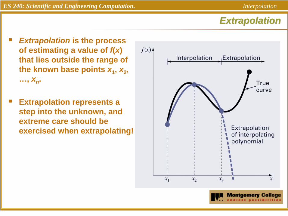
Extrapolation is the process of estimating a value of f(x) that lies outside the range of the known base points x1, x2, …, xn.

Extrapolation represents a step into the unknown, and extreme care should be exercised when extrapolating!


Extrapolation HazardsExtrapolation Hazards

World population using a 7th order polynomial extrapolation.


OscillationsOscillations

Higher-order polynomials can not only lead to round-off errors due to ill-conditioning, but can also introduce oscillations to an interpolation or fit where they should not be.

In the figures below, the dashed line represents a function, the circles represent samples of the function, and the solid line represents the results of a polynomial interpolation:


Introduction to SplinesIntroduction to Splines

An alternative approach to using a single (n-1)th order polynomial to interpolate between n points is to apply lower-order polynomials in a piecewise fashion to subsets of data points.

These connecting polynomials are called spline functions.

Splines minimize oscillations and reduce round-off error due to their lower-order nature.


Higher Order vs. SplinesHigher Order vs. Splines

Splines eliminate oscillations by using small subsets of points for each interval rather than every point. This is especially useful when there are jumps in the data:

a) 3rd order polynomialb) 5th order polynomialc) 7th order polynomiald) Linear spline

• seven 1st order polynomials generated by using pairs of points at a time


Spline DevelopmentSpline Development

a) First-order splines find straight-line equations between each pair of points that

• Go through the pointsb) Second-order splines find quadratic

equations between each pair of points that

• Go through the points• Match first derivatives at the interior

pointsc) Third-order splines find cubic

equations between each pair of points that

• Go through the points• Match first and second derivatives at

the interior points

Note that the results of cubic spline interpolation are different from the results of an interpolating cubic.


Spline DevelopmentSpline Development

Spline function (si(x))coefficients are calculated for each interval of a data set.The number of data points (fi) used for each spline function depends on the order of the spline function.


Cubic Splines Cubic Splines

While data of a particular size presents many options for the order of spline functions, cubic splines are preferred because they provide the simplest representation that exhibits the desired appearance of smoothness.

In general, the ith spline function for a cubic spline can be written as:

For n data points, there are n-1 intervals and thus 4(n-1) unknowns to evaluate to solve all the spline function coefficients.There is no ‘one equation’ that can represent the whole spline function on the domain

si x( )= ai + bi x − xi( )+ ci x − xi( )2 + di x − xi( )3


Piecewise Interpolation in MATLABPiecewise Interpolation in MATLAB

MATLAB has several built-in functions to implement piecewise interpolation. The first is spline:

yy=spline(x, y, xx)

This performs cubic spline interpolation


ExampleExample

Generate data:x = linspace(-1, 1, 9);y = 1./(1+25*x.̂ 2);

Calculate 100 model points anddetermine not-a-knot interpolationxx = linspace(-1, 1);yy = spline(x, y, xx);

Calculate actual function values at model points and data points, the 9-point (solid), and the actual function (dashed), yr = 1./(1+25*xx.̂ 2)plot(x, y, ‘o’, xx, yy, ‘-’, xx, yr, ‘--’)


MATLABMATLAB’’s s interp1interp1

FunctionFunction

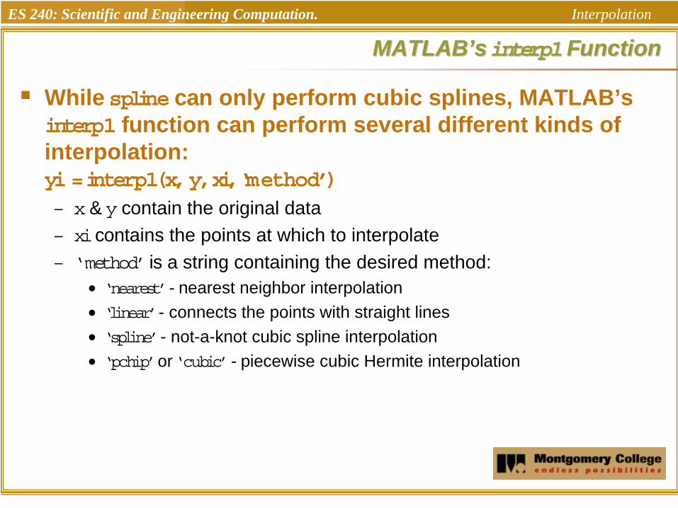
While spline can only perform cubic splines, MATLAB’s interp1 function can perform several different kinds of interpolation:yi = interp1(x, y, xi, ‘method’)–

x

& y

contain the original data–

xi

contains the points at which to interpolate–

‘method’

is a string containing the desired method:•

‘nearest’- nearest neighbor interpolation•

‘linear’

- connects the points with straight lines•

‘spline’

- not-a-knot cubic spline interpolation•

‘pchip’

or ‘cubic’

- piecewise cubic Hermite interpolation


LabLab

15.9

ES 240: Scientific and Engineering Computation....

Documents

Transcript of ES 240: Scientific and Engineering Computation....