A-A19 S ERUIA FILTER ARCHITECURES FOR TTLE NIUOEENT PH SE 1/11(u) SYSTOLIC SYSTEMS INC SAM JOSE CA 0 SATTERFIELD

WUEMSIFIED im9 RO60--mF/O 12/5 N

U Im II1 2.2

U.8

-11125 II'~ ~l1.6

MICROCOPY RESOLUTION TEST CHART

NATIONAL BUREAU OF $TANDATDS-1963-A

'? -'L

M~~tIE 001 P/ L~O SYSTOLIC SYSTEMS

AD-A195 526

KALMAN4 FILTER ARCHITECTURES FOR BATTLE MANAGEMENT

SBIR PHASE I E)TICCONTRACT DASG6-86-C-0056 S ECT E

Prepared for:

DEPARTMENT OF THE ARMY

OFFICE OF THE CHIEF OF STAFF

U.S. ARMY STRATEGIC DEFENSE COMMAND - HUNTSVILLE

P. 0. BOX 1500

HUNTSVILLE, ALABAMA 35807-3801

ATTN: DR. DOYCE SATTERFIELD

g Approved for A~

3 releQ

3 FINAL REPORT 420102, JANUARY 1987

I

8 T, 2 111I 40 NORTH FIRST STREET * SAN JOSE, CALIFORNIA 95131-2310 * 408/435-1760 * INT TELEX 184817 * FAX 408/287-4535

FOREWORDI3 - This report develops a comprehensive theory of parallel Kalman filtering

based on a unique decoupling principle permitting the predictor and corrector

equations in the filter to be computed in parallel. Highly parallel algorithms

and systolic architectures for efficiently implementing these advanced filter-

ing techniques are presented. The application of these methods to Strategic

Defense Initiative (SDI) target tracking problems is also described. - (This research was sponsored by the U. S. Army Strategic Defense Command

and conducted under U. S. Army contract number DASG60-86-C-0056. Dr. Doyce

Satterfield was the program manager at the U. S. Army Strategic Defense

Command - Huntsville.

Dr. Richard H. Travassos was the Principal Investigator at Systolic

Systems, Inc. Other members of the technical staff who contributed to this

project include Gary Lee and Larry Hubbart.

Accestor, For

NTIS CRA&IDTIC TAB Di

UBY.Diat repY.

Avt~~dj~

Jist

I %

Ag i'i'.y ..-?.,

I w

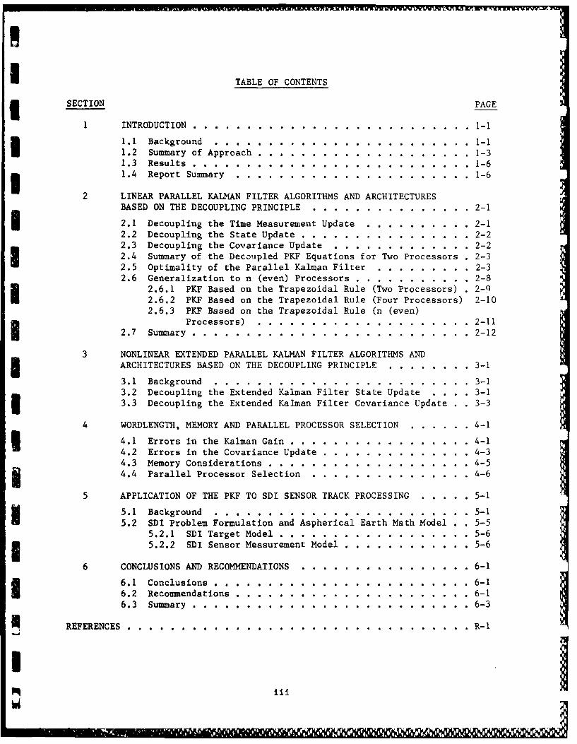
* TABLE OF CONTENTS

* SECTION PAGE

1 INTRODUCTION ............. .......................... 1-1

1.1 Background ............ ....................... 1-11.2 Summary of Approach ........ .................... . .1-31.3 Results ........... ......................... . .1-61.4 Report Summary ........ ...................... . .1-6

2 LINEAR PARALLEL KALMAN FILTER ALGORITHMS AND ARCHITECTURESBASED ON THE DECOUPLING PRINCIPLE ...... .............. . 2-1

2.1 Decoupling the Time Measurement Update ... .......... . 2-12.2 Decoupling the State Update ...... ................ .. 2-22.3 Decoupling the Covariance Update .... ............. .. 2-22.4 Summary of the Decoupled PKF Equations for Two Processors . 2-3

2.5 Optimality of the Parallel Kalman Filter ......... 2-32.6 Generalization to n (even) Processors ... ........... .. 2-8

2.6.1 PKF Based on the Trapezoidal Rule (Two Processors) . 2-9

2.6.2 PKF Based on the Trapezoidal Rule (Four Processors) 2-102.6.3 PKF Based on the Trapezoidal Rule (n (even)

Processors) ........ .................... . 2-11

2.7 Summary ........... ......................... .. 2-12

3 NONLINEAR EXTENDED PARALLEL KALMAN FILTER ALGORITHMS AND

ARCHITECTURES BASED ON THE DECOUPLING PRINCIPLE ........ 3-1

3.1 Background ...................... 3-1

3.2 Decoupling the Extended Kalman Filter State Update . . .. 3-13.3 Decoupling the Extended Kalman Filter Covariance Update . 3-3

4 WORDLENGTH, MEMORY AND PARALLEL PROCESSOR SELECTION . ..... .. 4-1

4.1 Errors in the Kalman Gain ...... .................. . 4-1

4.2 Errors in the Covariance Update ..... .............. .. 4-34.3 Memory Considerations ........ .................. .. 4-54.4 Parallel Processor Selection ...... .............. . 4-6

5 APPLICATION OF THE PKF TO SDI SENSOR TRACK PROCESSING .. ..... 5-1

5.1 Background ..... . ..... . . . . . . . .". . . . . 5-15.2 SDI Problem Formulation and Aspherical Earth Math Model . 5-5

5.2.1 SDI Target Model ...... .................. .. 5-65.2.2 SDI Sensor Measurement Model .... ............ . 5-6

6 CONCLUSIONS AND RECOMMENDATIONS ..... ................ .. 6-1

6.1 Conclusions ..... ..... ........................ .. 6-16.2 Recommendations ......... ...................... .. 6-16.3 Summary ........... .......................... .. 6-3

REFERENCES ................ ................................ R-1

iii

M

SECTION 1

INTRODUCTION

3 1.1 BACKGROUND

In navigation equipment, such as the GPS, a Kalman filter acts to smooth

3 data when the unit is unaided, or as an estimating filter when inertial data

are accepted. The need to integrate multiple sensors results in a hybrid

3 system with extremely large computational requirements for real-time applica-

tions. Often the hybrid system takes the form of a "cascaded" filter to ease

the computational burden. Sensor data integration is often difficult due to

correlating the time of the measurements and the different measurement rates

of the sensors. In this project, parallel Kalman filter architectures are

optimized for hybrid systems consisting of multiple sensors to achieve

improved performance. The computational advantage of parallel processing

minimizes measurement time sensitivity and data transfer over the bus. Thus,

multi-rate filtering is attainable via a unique decoupling of the predictor

* and corrector equations in the filter while maintaining optimal estimation.

The parallel processing techniques can be applied to real-time navigation,

a target tracking and scene analysis.

With recent developments in advanced sensors, a severe load has been

placed upon real-time signal processing systems to process large amounts of

data. Although the technology for implementing advanced sensors already

exists, the actual implementation depends strongly on the ability to develop

real-time signal processing hardware to process the data. Thus, to meet the

exceptionally high throughput requirements in DoD signal processing applica-

3 tions, considerable attention must be given to the development of highly

parallel (or systolic) signal processing architectures. Because signal

* processing architectures tend to be problem dependent to achieve the necessary

computational requirements, this project develops systolic signal processor

architectures which are well suited for recursive filtering, target tracking,

image processing and signal processing. The parallel architectures are based

on mapping the widely-used Kalman filter equations onto a generalized systolic

1-1

i array for linear and nonlinear parallel computation. Although this was

originally developed by Travassos (1982) for linear estimation on two (2)

processors, the extension of the method to n processors is the thrust of this

project.

roTo illustrate the need to extend the method for SDI sensor track proces-

sing via a Kalman filter consider the simplest case for linear filtering

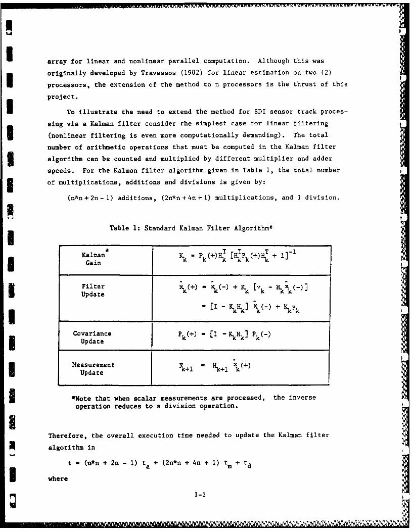
3 (nonlinear filtering is even more computationally demanding). The total

number of arithmetic operations that must be computed in the Kalman filter

Salgorithm can be counted and multiplied by different multiplier and adderspeeds. For the Kalman filter algorithm given in Table 1, the total number

3 of multiplications, additions and divisions is given by:

(n*n +2n- 1) additions, (2n*n +4n +1) multiplications, and 1 division.

Table 1: Standard Kalman Filter Algorithm*

Kalman N, Pk+H L*Kk /* + .IGain K k()"

Filte X.k()-y + K.k [vk - Hkk(-)](I" + v

kL Vk KC f

Covariance P [I - ,Hk]iUpdate kk k

Measurement c---Hkl~ (+)

3 *Note that when scalar measurements are processed, the inverseoperation reduces to a division operation.

Therefore, the overall execution time needed to update the Kalman filter

algorithm in

t - (n*n + 2n - 1) ta + (2n*n + 4n + 1) tm + tdI where

1-2

11. 5, "

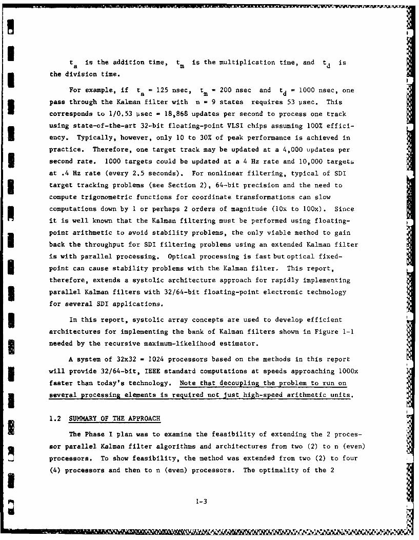
St a is the addition time, t. is the multiplication time, and td is

the division time.

For example, if ta = 125 nsec, tm - 200 nsec and td = 1000 nsec, one

pass through the Kalman filter with n - 9 states requires 53 psec. ThisIIcorresponds to 1/0.53 Usec - 18,868 updates per second to process one track

using state-of-the-art 32-bit floating-point VLSI chips assuming 100% effici-

ency. Typically, however, only 10 to 30% of peak performance is achieved in

practice. Therefore, one target track may be updated at a 4,000 updates per

second rate. 1000 targets could be updated at a 4 Hz rate and 10,000 target.

at .4 Hz rate (every 2.5 seconds). For nonlinear filtering, typical of SDI

3 target tracking problems (see Section 2), 64-bit precision and the need to

compute trigonometric functions for coordinate transformations can slow

computations down by 1 or perhaps 2 orders of magnitude (1Ox to 100x). Since

it is well known that the Kalman filtering must be performed using floating-

point arithmetic to avoid stability problems, the only viable method to gain

back the throughput for SDI filtering problems using an extended Kalman filter

is with parallel processing. Optical processing is fast but optical fixed-

point can cause stability problems with the Kalman filter. This report,

therefore, extends a systolic architecture approach for rapidly implementing

3 parallel Kalman filters with 32/64-bit floating-point electronic technology

for several SDI applications.

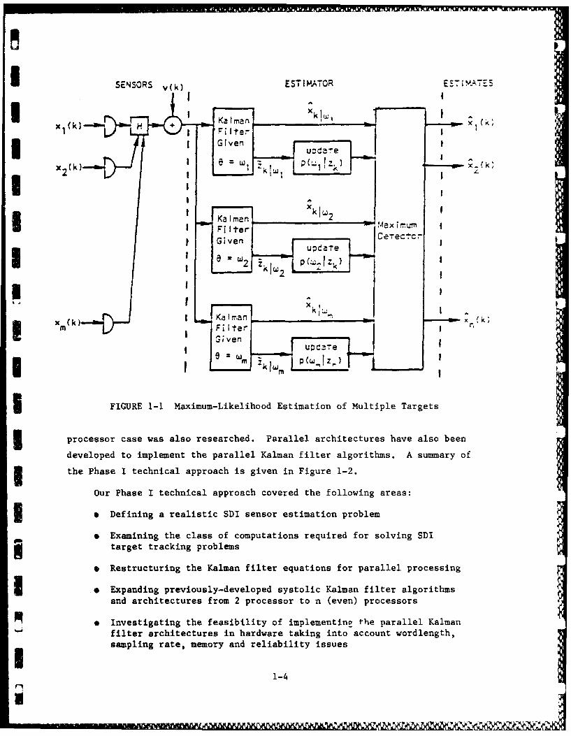
3 In this report, systolic array concepts are used to develop efficient

architectures for implementing the bank of Kalman filters shown in Figure 1-1

needed by the recursive maximum-likelihood estimator.

A system of 32x32 - 1024 processors based on the methods in this report

3 will provide 32/64-bit, IEEE standard computations at speeds approaching 1000x

faster than today's technology. Note that decoupling the problem to run on

3 several processing elements is reguired not just high-speed arithmetic units.

1*2 SUMMARY OF THE APPROACH

I The Phase I plan was to examine the feasibility of extending the 2 proces-

sor parallel Kalman filter algorithms and architectures from two (2) to n (even)

processors. To show feasibility, the method was extended from two (2) to four

(4) processors and then to n (even) processors. The optimality of the 2

1-3

iSENSORS v() ESTIATOR E57 I'!'TET

I " -I Kalman Xk[

Xl k 'Filter x k

I WI

devloed o mplmet teprl Kalman fite aloihs A1umar2o

I Filer a X i

Giv en upa.

C eTectc-

Ou hs ehia roc coee tefllwn aes

3 (k DenKal I man e pm R Filter I

WM(., I ,1 0

FIGUREI 1 MEnimum-Likelihood Estimation of Multiple Targets

processor case was also eresmrce ssr t ee have also been

developed to implement the parallel Kalman filter algorithms. A sumary ofi the Phase I technical approach is given in Figure 1-2.

Our Phase I technical approach covered the following areas:* Defining a realistic SDI sensor estimation problem

9 Examining the class of computations required for solving SDI~target tracking problems

* Restructuring the Kalman filter equations for parallel processing

* Ex panding previously-developed systolic Kalman filter algorithms

and architectures from 2 processor to n (even) processors

* Investigating the feasibility of implementing the parallel Kalman~filter architectures in hardware taking into account wordlength,

sampling rate, memory and reliability issues

1-4

i

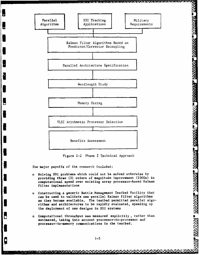
Parallel SDI Tracking MilitaryAlgorithms Applications Requirements

U . t

Kalman Filter Algorithms Based oni Predictor/Corrector Decoupling I

* I Parallel Architecture Specification

Wordlength Study, IMemory S izing

VLSI Arithmetic Processor Selection

I Benefits Assessment

U Figure 1-2 Phase I Technical Approach

U The major payoffs of the research included:

o Solving SDI problems which could not be solved otherwise byproviding three (3) orders of magnitude improvement (1000x) incomputational speed over existing array processor-based Kalmanfilter implementations

o a Constructing a generic Battle Management Testbed Facility thatcan be used to validate new parallel Kalman filter algorithmsas they become available. The testbed permitted parallel algo-rithms and architectures to be rapidly evaluated, speeding upthe deployment of new designs in SDI systems

o Computational throughput was measured explicitly , rather than Pestimated, taking into account processor-to-processor and -C

processor-to-memory comunications in the testbed.

g 1-5

1.3 RESULTS

The major results of the Phase I feasibility study can be summarized as

follows:

o The "optimality" of the parallel Kalman filter has been provenI analytically by showing that the dual (2) processor parallelKalman filter is "mathematically equivalent" to the standard(sequential) Kalman filter. The dual (2) processor parallelUKalman filter, however, executes twice as fast as the standardfilter since the predictor and corrector in the parallel Kalman

* filter can be computed in parallel.

o The parallel Kalman filter for linear estimation problems hasbeen extended from 2 to n (even) processors.

o Parallel architectures have also been developed to rapidlyimplement the linear parallel Kalman filter methods.

3o The wordlength, memory and VLSI arithmetic processor selectionshave been examined and documented.

o In addition to the above, the linear parallel Kalman filter hasbeen extended for nonlinear track processing. The extended,nonlinear parallel Kalman filter equations have been developedfor the 2 (and 4) processor case under Phase I. Under Phase 11,

th oliereteddpaallKalman filter can be furtherdecople an genralzedfor (een)processors.

1.*4 REPORT SUMMARY

3 The remainder of this report is organized as follows. The decoupling of

the parallel Kalman filter (PKF) for linear estimation is presented in Section

2. The optimality of the 2 processor linear PKF is proven analytically in

Section 2. The generalization of the two (2) processor linear PKF equations

to execute on nl (even) processors is also developed in Section 2. Nonlinear

U Kalman filtering via an extended parallel Kalman filter is presented in

Section 3. Parallel architectures for efficiently implementing the PFK

equations can be found in Sections 2 and 3. The wordlength, memory sizing

and VLSI arithmetic processor selection is given in Section 4. The SDI target

tracking problem is formulated in Section 5 for demonstrating the utility of

the PKF methods. Conclusions and recommendations for future work are pre-

sented in Section 6.

1-6

I M

SECTION 2

LINEAR PARALLEL KALMAN FILTER ALGORITHMS AND

ARCHITECTURES BASED ON THE DECOUPLING PRINCIPLE

The Kalman filter has been successfully applied to many signal processing

applications including target prediction, target tracking, radar signal

processing, on-board calibration of intertial systems and in-flight estimation I

of aircraft stability and control derivatives. The applicability of the

Kalman filter to real-time processing problems is generally limited, however,

by the filter's relative computational complexity. In particular, the number

of arithmetic operations required for implementing the Kalman filter with a

state variable grows as 0(n 2 ) for the time update and as 0(n 3 ) for the

covariance update. In general, real-time filtering cannot be performed on

large scale problems using a uniprocessor architecture because serious

processing lags can result (9). 0

The Kalman filter can be extended to a much greater class of problems by

using parallel processing concepts. Full utilization of parallelism can be

obtained through insight in the structure of the problem and decoupling of

arithmetic processes to permit concurrent processing.

To speed up Kalman filter computations, parallel processing is performed

at two levels: (1) the predictor and corrector equations of the Kalman filter

are decoupled so that the predictor and corrector can be computed on separate

processors, and (2) the measurement data are pipelined into each processor.

Therefore, both multiprocessing and pipelining are considered to achieve large

improvements in computational speed.

2.1 DECOUPLING THE TIME AND MEASUREMENT UPDATE

U The Kalman filter equations in Table 1-1 can be written in predictor-

corrector form as follows:

Predictor k_ k1kl+ 21

P - (+)oT (2.2)

2-1 p

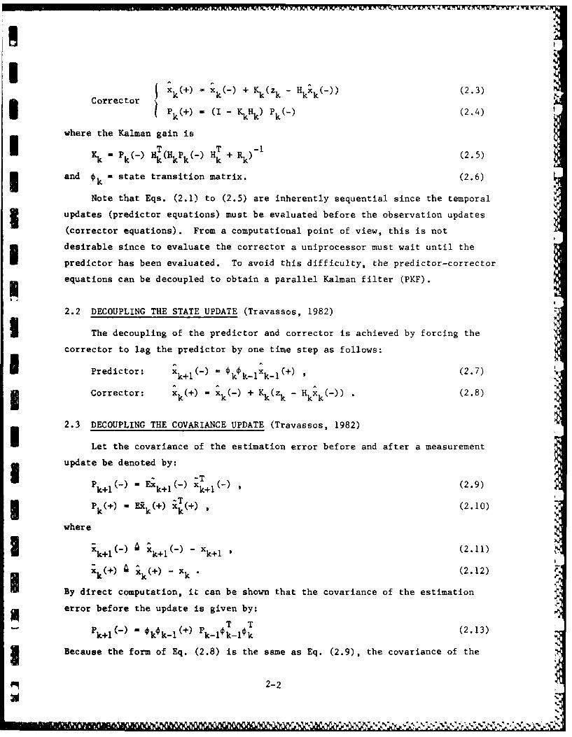
Corrector xk(+) Xk(-) + Kk(zk - HkXk(-)) (2.3)

S(+) I- KkHk) Pk(-) (2.4)

where the Kalman gain is

I k- ~ H(H P () H T + Rk) -1 (2.5)

and k- state transition matrix. (2.6)

Note that Eqs. (2.1) to (2.5) are inherently sequential since the temporal

updates (predictor equations) must be evaluated before the observation updates

(corrector equations). From a computational point of view, this is not

desirable since to evaluate the corrector a uniprocessor must wait until the

predictor has been evaluated. To avoid this difficulty, the predictor-corrector

equations can be decoupled to obtain a parallel Kalman filter (PKF).

2.2 DECOUPLING THE STATE UPDATE (Travassos, 1982)

The decoupling of the predictor and corrector is achieved by forcing the

corrector to lag the predictor by one time step as follows:

I Predictor: Xk+l k = kk Ixk i(+) , (2.7)

3Corrector: X k(+) x xk(-) + K.k(zk - H kxk(-~)) . (2.8)

2.3 DECOUPLING THE COVARIANCE UPDATE (Travassos, 1982)

Let the covariance of the estimation error before and after a measurement

update be denoted by:I -TPk+l (-)Ex k+l(-) ( - ) (2.9)

k1 k+ k+I Pk() - (+)£ +) ,(2.10)

where

3 k+l ,k+l - k+l (2.11)

k(+ ) Xk(+) _ Xk • (2.12)

I By direct computation, iL can be shown that the covariance of the estimation

error before the update is given by:

P - T T (2.13)

Because the form of Eq. (2.8) is the same as Eq. (2.9), the covariance of the

2-2

ND

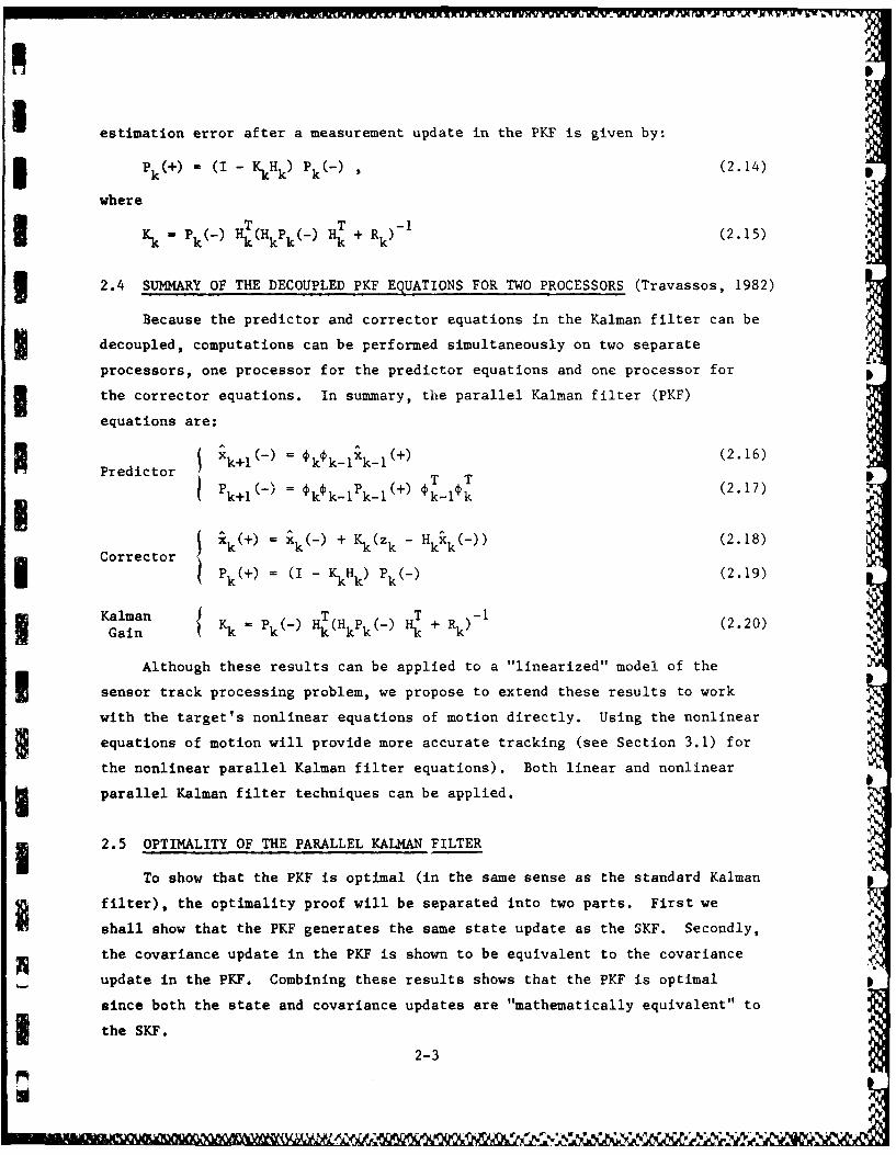
estimation error after a measurement update in the PKF is given by:

I k(+)- (I - KkHk) Pk(-) (2.14)

where

Kk - Pk- %(Hkpk(-) Hk + Rk)-1 (2.15)

3 2.4 SUMMARY OF THE DECOUPLED PKF EQUATIONS FOR TWO PROCESSORS (Travassos, 1982)

Because the predictor and corrector equations in the Kalman filter can be

decoupled, computations can be performed simultaneously on two separate

processors, one processor for the predictor equations and one processor for

the corrector equations. In summary, the parallel Kalman filter (PKF)

equations are:

Predictor xk+l (-) = kk-lk-1 (+) T T (2.16)

k+l ( - = k-Pk- ( + ) k-1k (2.17)

Corrector k xk(+) = Xk(- ) + Kk(zk - Hk k(-)) (2.18)

Fk(+) = (I - KkHk) ek ( - ) (2.19)

KamnT T -1 (220Gain Kk - Pk+ k ) (2.20)

Although these results can be applied to a "linearized" model of the

sensor track processing problem, we propose to extend these results to work

with the target's nonlinear equations of motion directly. Using the nonlinear

equations of motion will provide more accurate tracking (see Section 3.1) for

the nonlinear parallel Kalman filter equations). Both linear and nonlinear

parallel Kalman filter techniques can be applied.

2.5 OPTIMALITY OF THE PARALLEL KALMAN FILTER

To show that the PKF is optimal (in the same sense as the standard Kalman

filter), the optimality proof will be separated into two parts. First we

shall show that the PKF generates the same state update as the SKF. Secondly,

the covariance update in the PKF is shown to be equivalent to the covariance

update in the PKF. Combining these results shows that the PKF is optimal

since both the state and covariance updates are "mathematically equivalent" to

the SKF.

2-3

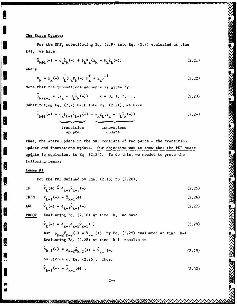
The State Update:

For the SKF, substituting Eq. (2.9) into Eq. (2.7) evaluated at time

k+l, we have:

ik+l ( - - kXk( - ) + kKk(zk - Hkk(-)) (2.21)

where

Kk H (HkPk(-) HT + Rk) 1 (2.22)

I Note that the innovations sequence is given by:

Zk/k+1 - (zk - Hkxk(-)) k - 0, 1, 2, ... (2.23)

Substituting Eq. (2.7) back into Eq. (2.21), we have

x (k+1 (-) f k-kkl (+) + 4 kKk(Zk - Hkk(-)) (2.24)

transition innovationsupdate update

Thus, the state update in the SKF consists of two parts - the transition

update and innovations update. Our objective was to show that the PKF state

update is equivalent to Eq. (2.24). To do this, we needed to prove the

following lemma:

Lemma #1

For the PKF defined by Eqs. (2.16) to (2.20),

IF xk(+) k-xk 1(+) (2.25)

THEN Xk-I (=

- ) (2.26)

AND xk( - ) - k-iXkl ( - ) (2.27)

PROOF: Evaluating Eq. (2.16) at time k, we have

I k(-) - Ok-lok2Xk-2(+) (2.28)

But _ (+) - x (+) by Eq. (2.25) evaluated at time k-.

Evaluating Eq. (2.28) at time k-i results in

k-1 ( - ) - Ok-2^k_2(+) Xkl(+)2.29)

by virtue of Eq. (2.25). Thus,

x kl ( - ) - Xk I ( + ) . (2.30)

2-4

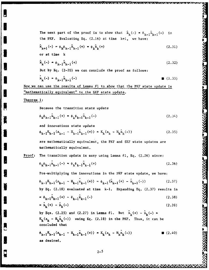
The next part of the proof is to show that (- = k-l k-1(~ in

the PKF. Evaluating Eq. (2.16) at time k+1, we have:

k(-) - k-k1 k1(+) = tkk (2.31)

or at time k

xk(-) - k-1Xk-1(+) (2.32)

U But by Eq. (2-20) we can conclude the proof as follows:

Xk(-) = Ik1X kl(-) U (2.33)

Now we can use the results of Leimma #1 to show that the PKF state update is

"1mathematically equivalent" to the SKF state update.

Theorem 1:

Because the transition state update

kI k-kl(+) - k-k-l(-) (2.34)

and innovations state update

K-( -H x (+)=K(z - H(2.35)ok-i K-i~k- k-i k-i() K

are mathematically equivalent, the PKF and SKF state updates are

mathematically equivalent.

Proof: The transition update is easy using Lemma #'1, Eq. (2.26) since:

3k- A-( - AkIkl+ (2.36)

Pre-multiplying the innovations in the PKF state update, we have:

ok-1Kk-1(zk-1 - H k-1x ki(+)) = - ( k- xkl(-)) (2.37)

U by Eq. (2.18) evaluated at time k-i. Expanding Eq. (2.37) results in

3 - ~k-k(+) - k1 k1l(-) (2.38)

- xk( - Xk(-) (2.39)

by Eqs. (2.25) and (2.27) in Lemma #1. But x - )

K.k(zk - H kxk(-)) using Eq. (2.18) in the PKF. Thus, it can be

concluded that

Ok-1Kk-i(zk-1 - H - -() - K~k(zk - Hkxk(-)) U (2.40)

3 as desired.

g 2-5

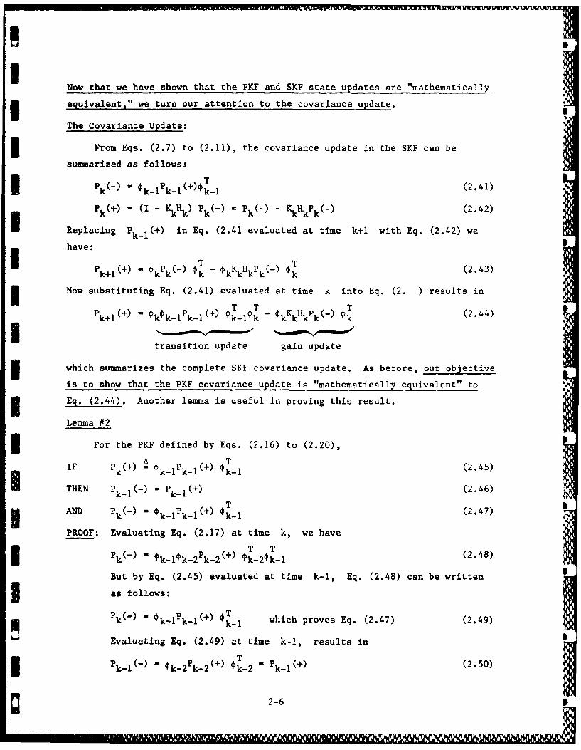
Now that we have shown that the PKF and SKF state updates are "mathematically

equivalent," we turn our attention to the covariance update.

The Covariance Update:

From Eqs. (2.7) to (2.11), the covariance update in the SKF can be

summarized as follows:

U Pk ( - ) k k-Ik-1 ()k-1 (2.41)

P - (I - KkHk ) Pk ( - ) - Pk ( - ) - KkHkPk(- ) (2.42)

Replacing Pk-l(+) in Eq. (2.41 evaluated at time k+1 with Eq. (2.42) we

have:I T .T

k+1 k k kKkHkPk() k (2.43)

Now substituting Eq. (2.41) evaluated at time k into Eq. (2. ) results in

P T T _ KkHkT (2_44)k+l (+ ) = kk-IPk-l(+) Ok- 1k kPk() k(2.44)

transition update gain update

which summarizes the complete SKF covariance update. As before, our objective

is to show that the PKF covariance update is "mathematically equivalent" to

Eq. (2.44). Another lemma is useful in proving this result.

Lemma #2

For the PKF defined by Eqs. (2.16) to (2.20),T

IF Pk k-Ik-1( ) 0k-1 (2.45)

THEN Pk-l (- ) Pk-l(+) (2.46)

AND Pk- W+ T (2.47)k k-1 k-1~~ k-1

PROOF: Evaluating Eq. (2.17) at time k, we have

P - _ ) T T (2.48)I k - k-1k-2pk-2(~ *k-20k-1(248

But by Eq. (2.45) evaluated at time k-i, Eq. (2.48) can be written

as follows:

Sk-I which proves Eq. (2.47) (2.49)

Evaluating Eq. (2.49) at time k-1, results in

P T (+) (2.50)Pk-I ( - ) =k-2Pk-2 ( + ) k-2 k-1

2-6 0

.-. ... :T R I; , , .

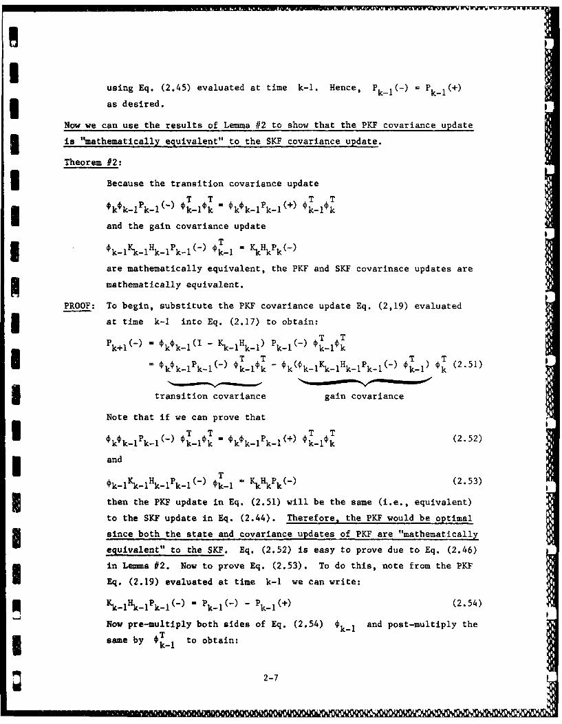
musing Eq. (2.45) evaluated at time k-i. Hence, Pk-1- ) = k W

as desired.

Now we can use the results of Lemma #2 to show that the PKF covariance update

is "mathematically equivalent" to the SKF covariance update.

Theorem #2:

Because the transition covariance update

T T T Tkk-lPk-l(_ k-1k - Yk-kIk kk_Ik

and the gain covariance update

I C~k-l Ik-IPk-i (- ) k _-1 kkk(- )

are mathematically equivalent, the PKF and SKF covarinace updates are

* mathematically equivalent.

PROOF: To begin, substitute the PKF covariance update Eq. (2,19) evaluated

at time k-I into Eq. (2.17) to obtain:

Pk+l (- ) = kk-I( - KkHk I ) Pk-I ( - k-kk

() T T - k -% HT T' k- -l k_-14 k -- p-l- k-1 k (.1

i transition covariance gain covariance

Note that if we can prove that

Y A- k_1k Y A-()0T 0T =+)0T_ T (2.52)

andIk, T (.3*k-lKk-1Hk-k-l1(-) k-I - KkHkPk() (2.53)

3then the PKF update in Eq. (2.51) will be the same (i.e., equivalent)

to the SKF update in Eq. (2.44). Therefore, the PKF would be optimal

since both the state and covariance updates of PKF are "mathematically

equivalent" to the SKF. Eq. (2.52) is easy to prove due to Eq. (2.46)

in Lemma #2. Now to prove Eq. (2.53). To do this, note from the PKF

Eq. (2.19) evaluated at time k-I we can write:

Kk-lHk-lPk-1(- ) " Pk-1 (- ) - Pk-1 (+ ) (2.54)

Now pre-multiply both sides of Eq. (2.54) k-I and post-multiply the

same by to obtain:

2-7

*

k-IKk-IHk-Pk-( -) (k- =H - P T-I (2.55)

T - T _ ( .6

k-1 k-1 k-1 - Ok- -(2.56)

f k(-) - Pk(+) KkHkPk(-) (2.57)

from Lemma #2 and Eq. (2.19) of the PKF. Therefore, we have shown

that

0k-1Kk-1Hk-1Pk-1(-) k-1 - KkHkPk(-) (2.58)

Summary

This section demonstrates the parallel Kalman filter, originally

developed by Travassos (1985), based upon decoupling the filter's predictor

and corrector equations, is optimal in the same sense as the standard Kalman

filter. This was proven via two lemmas and two theorems. Since the PKF

method can be extended to more than two processors, it is anticipated that

the optimality proof can be extended as well. Furthermore, extending the

results to nonlinear filtering is also anticipated to be successful.

2.6 GENERALIZATION TO n (EVEN) PROCESSORS

Now that the stability and convergence of the two-processor parallel

Kalman filter (PKF) has been analytically investigated and shown to be"mathematically equivalent" to the standard Kalman filter (SKF), we now focus

3 our efforts on extending the PKF algorithm to run on n (even) processors. Our

approach is based on the principle of induction; i.e., we develop the two-

processor then the four-processor case and then by induction generalize the

method for n (even) processors.

3 To provide a more accurate solution, the generalized method is based on

the trapezoidal rule of numerical integration rather than Euler integration

which has been used to date. The Kalman filter update is then accurate to

0(h2) rather than 0(h). The additional accuracy is important because it is

anticipated that the integration step size, h, will be large due to the

computational complexity of the Kalman filter equations. For example, with a

sample rate of 100 Hz, the Euler-integration-based PKF would be accurate to

0(h) - 0.01, while the trapezoidal-rule-based PKF would be accurate to

0(h 2) - 0.0001 (i.e., as accurate as the 12-bit sensor data).

2-8

U

2.6.1 PKF Based on the Trapezoidal Rule (Two Processors)

3 The trapezoidal rule for integrating a set of ordinary differential

equations is given by:

3 Xk+1 - xk + h(f(xk,tk) + f(xk+1,tk+l)) (2.59)

where x is the solution of the ode, f(xt) is the right-hand-side (RHS) of

3 the initial value problem and h - tk+1 - tk is the integration step size.

The trapezoidal rule is an implicit method since Xk+1 appears implicitly on

the RHS of Eq. (2.59). Note that f(x,t) can be, in general, a nonlinear

function or linear such as f(xt) - Fx(t). To solve Eq. (2.59), a predictor

3 is needed of the form below to estimate Xk+ I .

Xk+1 - xk + hf(xk,tk) (2.60)

Hence, combining Eqs. (2.59) and (2.60), we obtain a predictor-corrector

method based on the trapezoidal rule:

Predictor: x+ = xc + hf(Xc) (2.61)k+1 k k' k

Corrector: x k+ h(f(xck) + f(x t)) (2.62)

Note that the predictor must be evaluated before the corrector equation can be

computed. A parallel predictor-corrector (PPC) method has been derived by

Miranker (1967) that allows the predictor and corrector to be evaluated

simultaneously on two (2) processors as follows:

Parallel Trapezoidal Rule (Two Processors):

3 Predictor: Xk+l. Xk-Ci + 2hfP (2.63)

Corrector: xc xc_ + h(f p + fc) (2.64)

k k-i k k-i3 where fP - f(x,k) and fk-l - f(x_ 1 ,k-1).

In the special case when fp - *kxk(-) is the RHS of the Kalman filter

state update before a measurement and G - lk ( -KkH Tk is thesttek k (IlKHk) Pk (-)(I k) Ok i hRHS of the covariance update before a measurement, then the two (2) processor

3 parallel Kalman filter can be derived as follows:

Parallel Kalman Filter Based on Trapezoidal Rule (Two Processors)

Predictor: xk+l(-) - Xk-l(+) + 2hOkXk(-) (2.65)

Sk+ - P ( + ) + 2hGP (2.66)

k 2 -9

IwhereGp Kk T T(2.6)

wr k p - KkHk)Pk() + Pk - Kk k ) k(2.6)

UCorrector: xk(+) - Xk-1+ + h) 2(4 k k (-) + 4k-1 xk-1(+)) + Kk(zk-H k k (-)) (2.68)

PW+- P + + h/2(Gp + G ) - (2.69)k k 1k k 1 K H k ) T 0 T ( . 0where G - Ok(i - KkHk)Pk(_) + pk( -)(1 _ KkHk) (2.70)

Gk-1 = Ok-lPk-l(+) + Pk-1 ( (2.71)

In the above PKF, the (-) notation represents a value before a measurement

update and the (+) notation is a value after a measurement update. Similarly,

the p for predictor corresponds to the (-) notation and the c for corrector

value corresponds to the (+) notation.

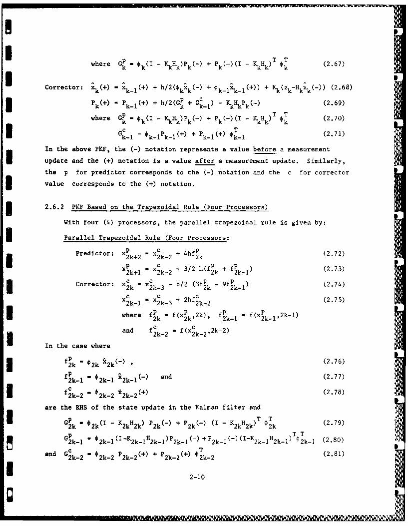
2.6.2 PKF Based on the Trapezoidal Rule (Four Processors)

With four (4) processors, the parallel trapezoidal rule is given by:

Parallel Trapezoidal Rule (Four Processors:

Predictor: xp c + 4hfp (2.72)2k+2 - x2k-2 2k

2k+l 2k-2 + 3/2 h(fk + fk (2.73)

Corrector: xc h12 (3fP k- 9f (2.74)Corco 2k X2k_32k k-

c c 2 hf'k 2 (2.75)X2k-1 =2k-3 2-

where f2k f f(xPk,2k),2k-I = f(xPk-l2k-1)

and f c f~c 2k )I 2k-2 = f (X2 k-2,k 2

In the case where

fP k (2.76)A 2k ^2

f - " 2k-1 X2k-1~ and (2.77)

U2k-2 1 2k-2 2k-2

are the RHS of the state update in the Kalman filter and

GP '2k (I - K Hk) P (-) + P (-) (I - K H T T (2.79)2k 22k 2k A 2k 2kH2k 2k

P(IT T2k-i "02k-1l 2k-2k-1 k- P 2k1(2k-

k -1 ) 2k-1 (2.80)

and Gc P W + W (2.81)2k-2 2k-2 2k-2 2k-2 2k-2

I 2-10

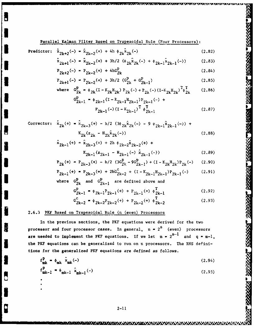
Parallel K~alman Filter Based on Trapezoidal Rule (Four Processors):

UPredictor: X^2k+2 ^ 2- 2 ( + 4h 4 2k 2k(~ (2.82)

x 2k+i(-) -x 2k-2 (+) + 3h/2 ( 2xk- + 2k-1x 2k-1(-)) (2.83)

2k+2 - 2k-2 ~~ 2khG

P () + h2k(P+G (2.84)~2k+1 ~ ~2k-2~~ h2(+G 2k 2k-i12.5

where GV (I-K(-K H TT (.62k 2k(I 2 020H2k) - +p (- 2k02k~ 2k (.6

2k- 2k- +k12-12-

2k-1()I 2k-1) 4'2k-1 2.7

Corrector: x 2k (+) x x2k-3 (+) -h/2 (3 2kX2k(-) - 2- x 2kl( +

K K2k(z 2k H H2kx2k(-)) (2.88)

3 2ki(+ =2k-3 (l) + 2h 2k-2x2k-2+ + (.9

K 2 k-1(z 2 k-1 - H 2 k-l() 2kl(-)) (.9

= + - h/2 (3Gp 9GP )kI -K kH k)p~ (2.90)2k2- 2k 2k- 2k +k 2k

P P2k(3+) + 2hG,,c + (I -K kH k)Pkl ) (2.91)

Iwhere GP and Gp are defined above and2k 2k-i

2k-i = k-l +-l2k-1~~ 2k-1 (.2

G c P W k+2P W T (2.93)2k22k-2 2k- 2k- 2k-2

2.6.3 PKF Based on Trapezoidal Rule (n (even) Processors

In the previous sections, the PKF equations were derived for the two

3processor and four processor cases. In general, n - 2 s (even) processors

are needed to implement the PKF equations. If we let m - 28S1 and q - m1

the PKF equations can be generalized to run on n processors. The RHS defini-

tions for the generalized PKF equations are defined as follows.

3 fp Ank ck- (2.94)

fp M mk- (2.95)

g 2-11

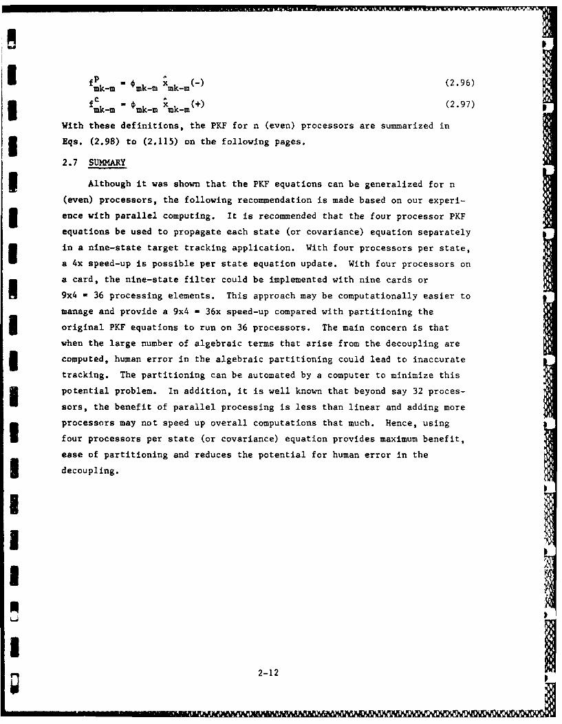
fP - = (2.96)mk- ¢mk-m ,k-m ( -) (.

fC - + (2.97)3mk-m = mk-m mk-m( 2.

With these definitions, the PKF for n (even) processors are summarized in3 Eqs. (2.98) to (2.115) on the following pages.

2.7 SUMMARY

Although it was shown that the PKF equations can be generalized for n

(even) processors, the following recommendation is made based on our experi-

ence with parallel computing. It is recommended that the four processor PKF

equations be used to propagate each state (or covariance) equation separately

in a nine-state target tracking application. With four processors per state,

a 4x speed-up is possible per state equation update. With four processors on

a card, the nine-state filter could be implemented with nine cards or

9x4 - 36 processing elements. This approach may be computationally easier to

manage and provide a 9x4 = 36x speed-up compared with partitioning the

3 original PKF equations to run on 36 processors. The main concern is that

when the large number of algebraic terms that arise from the decoupling are

3 computed, human error in the algebraic partitioning could lead to inaccurate

tracking. The partitioning can be automated by a computer to minimize this

3 potential problem. In addition, it is well known that beyond say 32 proces-

sors, the benefit of parallel processing is less than linear and adding more

processors may not speed up overall computations that much. Hence, using

four processors per state (or covariance) equation provides maximum benefit,

ease of partitioning and reduces the potential for human error in the

* decoupling.

,II

2-12

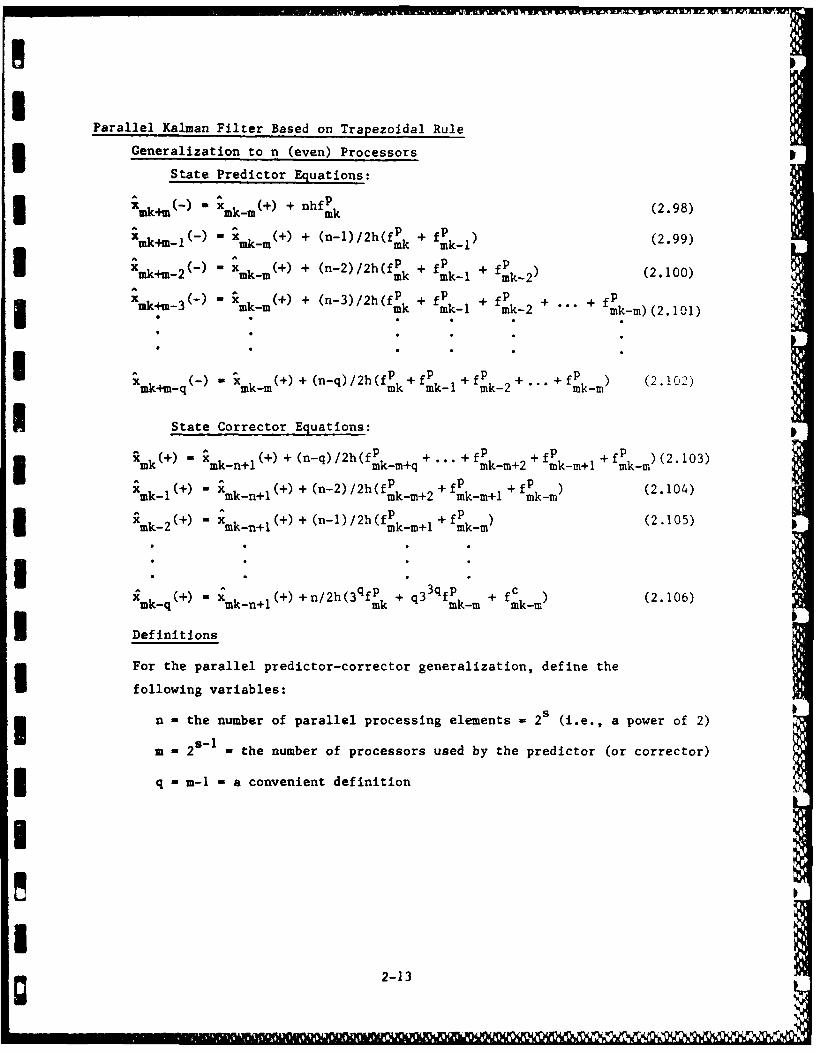
IParallel Kalman Filter Based on Trapezoidal Rule

Generalization to n (even) Processors

State Predictor Equations:- xm _m(+) + nhf k (2.98)3 xik4 n( in-r

nk~m~(-) W X (+) + (n-l)/2h(fp + fPk) (2.99)xm|- mk- ^ mk-Inkn-2( -) " Xmk~(+) + (n-2)/2h(fP + fP + fP (2.100)

ink ink-i ink-2 (2. " 2W + (n-3)/2h(fP + fP + fP + + fP

iik k-3n - mk-i mk-2 " nk-m)(2.101)

m +(n-q)/2h(f p +fP +fP + .. fPXmk-+m -q- m k -m(+ mk mk-1 mk-2 mk-m

I State Corrector Equations:

S ( (n-q)/2h(fPk + + fp + f P +fP )(2.103)

- X .+ rnrnq + .. ik-m--2 nk-n-i- ik-rn(+)+(n-2)/2h(f ^+fP +fP ) (2.104)

mk-+ mk-n+l +k) m-+2 mk-m+i mk-m

W - x (+) +(n-i)/2h(fP +f (2.105)I rk-2 ink-n+jI ink-in+i k

° (+) +) . h/2 h(3 lf + q3 __ + f ) (2.106)rnk-q inn~ k 'ik-in ink-r

* Definitions

For the parallel predictor-corrector generalization, define the

following variables:

n - the number of parallel processing elements - 2s (i.e., a power of 2)

m - 2 - the number of processors used by the predictor (or corrector)

q - m-1 -a convenient definition

2

g 2-13 }

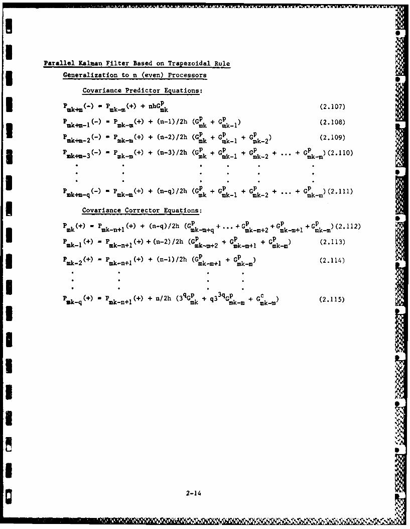
Parallel Kalmnan Filter Based on Trapezoidal Rule3 Generalization to n (even) Processors

Covariance Predictor Equations:

P P + + nk (2.107)

P - m~m+ (n-1)/2h (Gp + G 218mm - +ik ink-1(.18

mku -2 mk m- kPkm+ + (n-2)/2h (GP + GP + 219

-m~m+ + (n-3)/2h G + p + GP + .. + GP )(2.110)inm- k ink-i ik-2 ink-in

p +) n-)2 (GP GP +G+ + GP )(2.111)ink-in-q(- - ink-in + n)h ik ink-i ik-2 in-in

Covariance Corrector Equations:

IPn() Pkni() (n-q)/2h (Gp + +Gp +GP G (212

( in-+)~ + (n-2)/2h (GP + Gp + Gp (2.113)inI kn+ k-in+2 ink-rn-H ik-in

(+ in- + (n-1)/2h (GP + GP (214Ik- - - + ink-w+l ink-in(.14

I PP . (+) knl~ + n/2h (3 qGP~ + q3 3q Gp + Gck..n (2.115)

Iu- knlm km m-

g 2-14

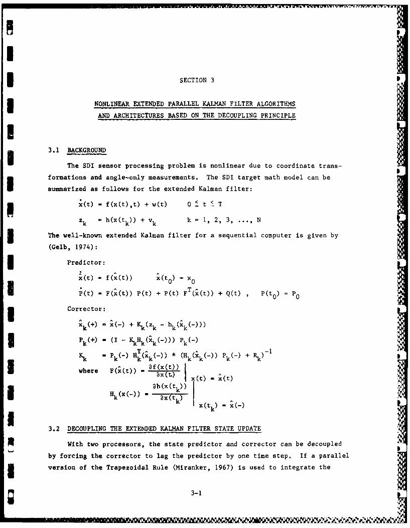
ISECTION 3

NONLINEAR EXTENDED PARALLEL KALMAN FILTER ALGORITHMS

AND ARCHITECTURES BASED ON THE DECOUPLING PRINCIPLEI3.1 BACKGROUND

The SDI sensor processing problem is nonlinear due to coordinate trans-

formations and angle-only measurements. The SDI target math model can be

summarized as follows for the extended Kalman filter:

x(t) - f(x(t),t) + w(t) 0 < t <. T

zk - h(x(tk)) + vk k = 1, 2, 3, ... , N

3 The well-known extended Kalman filter for a sequential computer is given by

(Gelb, 1974):

* Predictor:

x(t) - f(x(t)) x(t0) t 0

iP(t) - F(x(t)) P(t) + P(t) FT(x(t)) + Q(t) P(t0 = 0

Corrector:

k(+) x x(-) + Kk(zk - hk(Xk(-)))

I Pk(+) - (I- KkHk(Xk(-))) Pk ( - )T (^ 1

Kk - Pk - Hk(xk(-)) (k(Xk P ( - ) + Rk)-

I where F(x(t)) af(x(t))

ax(t) t) - x(t)

Ih(x(tk))H k ( X ( ) ) = X ( t k ). -

Sx(tk x (-)

3.2 DECOUPLING THE EXTENDED KALMAN FILTER STATE UPDATE

U With two processors, the state predictor and corrector can be decoupled

by forcing the corrector to lag the predictor by one time step. If a parallel

3 version of the Trapezoidal Rule (Miranker, 1967) is used to integrate the

3-1

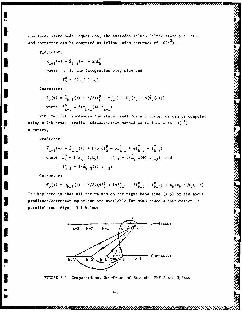
I nonlinear state model equations, the extended Kalman filter state predictor

and corrector can be computed as follows with accuracy of O(h ).2

Predictor:

x - Xk-(+) + 2hfPIk+1 k- kwhere h is the integration step size and

IfP .f(: (-,

Corrector:

k(+) + h/2(fp + fc_ + -

where f c_ -f(Xk1(+),t-~ kz

With two (2) processors the state predictor and corrector can be computed

using a 4th order Parallel Adams-Moulton Method as follows with O(h 4

accuracy.

3 Predictor:

xk+1 (-)" xkl+) + h/3(8fp - 5f'_ + 4fc_ - f _)

where fP - f(xk(-)tk) 2 f(xk (+),t and

f-3 - f(xk-3(+)'tk-3)

Corrector:

Xk(+) - Xkl(+) + h/24(9fP + 19f - 5f -2 + fk-3) + K(zk -h(Xk(-)))

The key here is that all the values on the right hand side (RHS) of the above

predictor/corrector equations are available for simultaneous computation in

parallel (see Figure 3-1 below).

I redicor

--- Correctora!k-3 kt k--'- k+l ,

3 FIGURE 3-1 Computational Wavefront of Extended PKF State Update

3-2

_ _ _ _ _ _ _ _ _ _ _ _ _ _ _ _ _ _ _ _ _ _ _ _ _ _X__ _

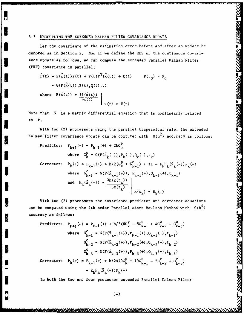
3.3 DECOUPLING THE EXTENDED KALMAN FILTER COVARIANCE UPDATE

Let the covariance of the estimation error before and after an update be

denoted as in Section 2. Now if we define the RHS of the continuous covari-

ance update as follows, we can compute the extended Parallel Kalman Filter

(PKF) covariance in parallel:

3i(t) - F(x(t))P(t) + P(t)FT x(t)) + Q(t) p(t 0 P p0

- G(F(x(t)),P(t),Q(t),t)

wher e F (i (t)) - af ( (t))

a t) I x(t) i(t)

Note that G is a matrix differential equation that is nonlinearly related* to P.

With two (2) processors using the parallel trapezoidal rule, the extended

Kalman filter covariance update can be computed with 0(h 2) accuracy as follows:

Predictor: P H i P (+) + 2hGp

where Gp - G(F( k(_))I (-I (-)It)

Corrector: P (+ + + h/2(GP + Gc ) + (I -KkHk(k~)k~

where k-i =- G(F( k(+)), Pkl(+),Qki(+),tki

and Hkk() - h(x(t k)ax(t k)

Ix(t k) =k(-)

With two (2) processors the covariance predictor and corrector equations

can be computed using the 4th order Parallel Adams Moulton Method with 0(h 4

accuracy as follows: p-5 GPredictor: P k Cl-) - Pk1 + + h/3(8G~ - k-i I 4Cc - G k 3 )

where GCc = -~ (),I k i .Xk1 +Ik-1\+)Qk-1(+tki/

k-2 - (~k 2 'k-2(+) '~k-2(+),tk-2)

- ~k 3 (k-3 ,k-3(+),Qk-3(+)ttk-3

Corrector: P+)- () + k/4(G + k-ic - 5 C + G c)

K Kk Hk (k(D)Pk(-)

In both the two and four processor extended Parallel Kalman Filter

3-3

equations, the Kalman gain is computed as follows:

Kalman Gain: Pk(-)HT(k(-)(Hk (k())pk()Hk(k()) + R-1

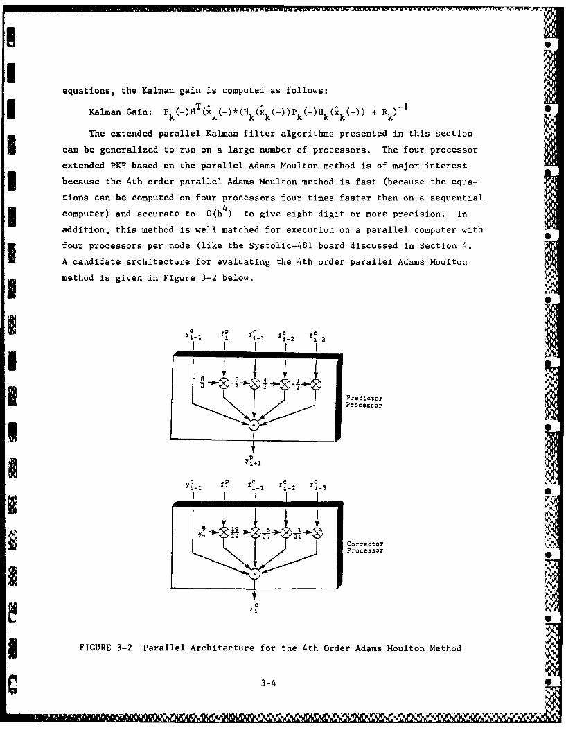
The extended parallel Kalman filter algorithms presented in this section

can be generalized to run on a large number of processors. The four processor

extended PKF based on the parallel Adams Moulton method is of major interest3 because the 4th order parallel Adams Moulton method is fast (because the equa-

tions can be computed on four processors four times faster than on a sequential

computer) and accurate to 0(h 4) to give eight digit or more precision. In

addition, this method is well matched for execution on a parallel computer with

four processors per node (like the Systolic-481 board discussed in Section 4.

A candidate architecture for evaluating the 4th order parallel Adams Moulton

method is given in Figure 3-2 below.

Yc P f fC 10i- I i- 1 -2 1-3

i I I I I

5 4

Predictor

Processor

• .

C_ 1 P 1 C- c

YiI I I I 2 i -

9 10 5_ 1

correctorProcessor

FIGURE 3-2 Parallel Architecture for the 4th Order Adams Moulton Method

3-4 SC N

I

SECTION 4

WORDLENGTH, MEMORY AND PARALLEL PROCESSOR SELECTION

Before implementing the parallel Kalman filter algorithms and architec-

tures derived previously in this report, it is of interest to examine the

wordlength, memory and timing requirements for these methods. The timing

requirements, in particular, have a direct impact on the selection of the

VLSI arithmetic processors used for computation. Memory speed and bus con-

siderations also impact overall system throughput. To start, wordlength

* considerations are analyzed first.

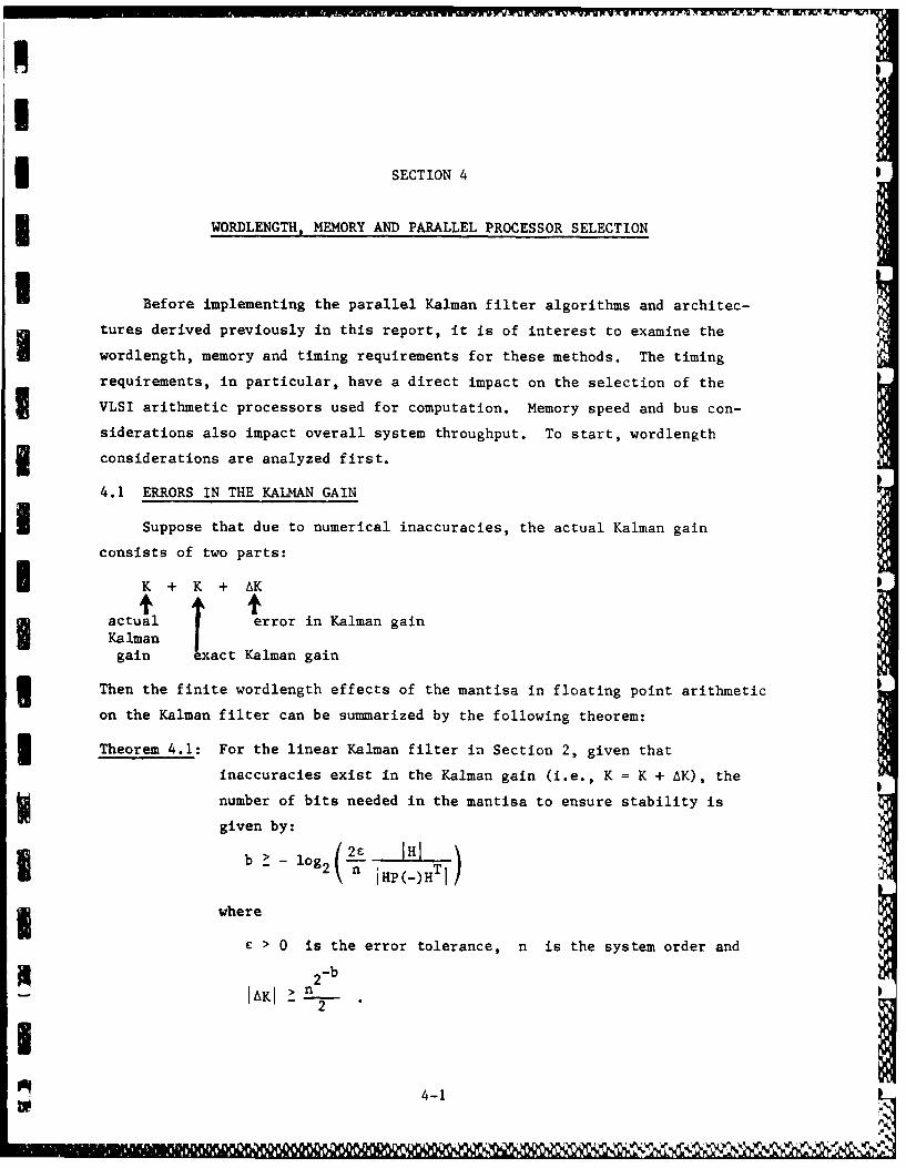
4.1 ERRORS IN THE KALMAN GAIN

U Suppose that due to numerical inaccuracies, the actual Kalman gain

consists of two parts:

I K + K + AK

actual error in Kalman gainKalmangain exact Kalman gain

Then the finite wordlength effects of the mantisa in floating point arithmetic

on the Kalman filter can be summarized by the following theorem:

Theorem 4.1: For the linear Kalman filter in Section 2, given that

inaccuracies exist in the Kalman gain (i.e., K = K + AK), the

number of bits needed in the mantisa to ensure stability is

given by:

Ib 2c_-H102- n iHp(_)H Ti

* where

£ > 0 is the error tolerance, n is the system order and

2-

4-1

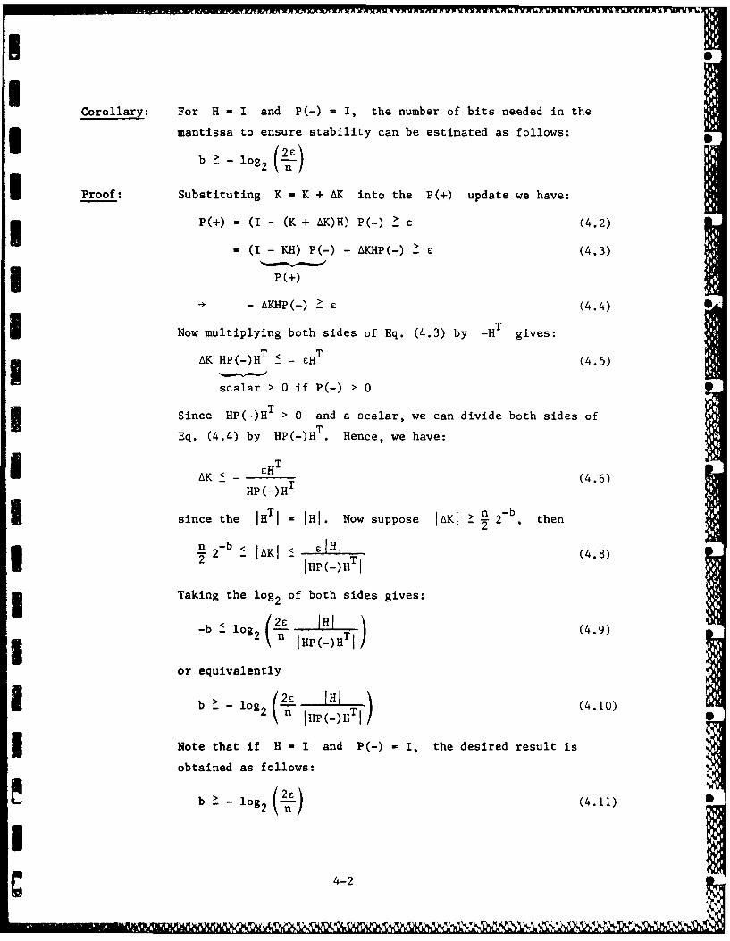
Corollary: For H - I and P(-) - I, the number of bits needed in the

mantissa to ensure stability can be estimated as follows:

b - log2

I Proof: Substituting K - K + AK into the P(+) update we have:

3 P(+) - (I - (K + AK)H) P(-) _> c (4.2)

- (I - KH) P(-) - AKHP(-) > c (4.3)

P (+)

4 - AKHP(-) > (4.4)

Now multiplying both sides of Eq. (4.3) by -HT gives:

AK HP(-)HT < - HT (4.5)

scalar > 0 if P(-) > 0

Since HP(-)HT > 0 and a scalar, we can divide both sides of

Eq. (4.4) by HP(-)H T . Hence, we have:

AK < c THT (4.6)HP (-)HT

since the IHTI = IHI. Now suppose JAKI a 1 2b, then

2-b < HAKI EIH (4.8)2 IHP(-)HTI

Taking the log 2 of both sides gives:

-b < log2 (2 IH )T) (4.9)- n IHp(_)HT

or equivalently

b (2 H(_)HTI (4.10)

Note that if H - I and P(-) - I, the desired result is

obtained as follows:

b 09 ( o 2 ) (4.11)

I4-4-2

3 24

18 C 1-

~12 C1-

6

20 40 60 801012

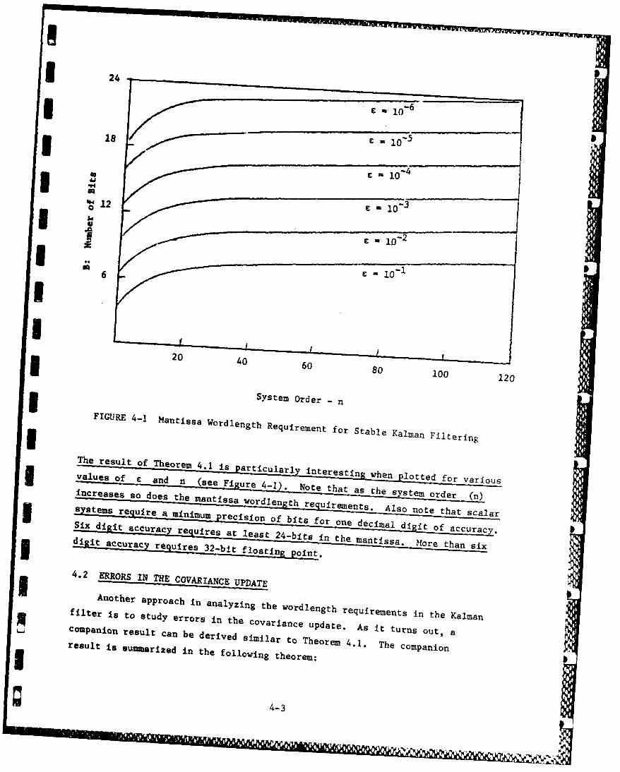
System Order -nFIGURE 4-1 Mantissa Wordlength Requirement for Stable Kalman Filtering

The result fhoe 4.1 -is Particularly interesting whenotefrvai s

3 values f and n (see Fiure 4-1). Note that as the sstem order (n)increases s d o st e antissa wordlength requirements A lso note that scalar

3 Systems reuie a miimm precision of bits for one decimal diitoacucySix digit accuacy euires t least 2 4-bits in the nis orth n sixg di it accurac reuires 32-bit floating oint.

4.2 ERRORS IN THE COVARIANCE UPDATE

Another approach in analyzing the wordlength requirements in the Kalmanfilter is to study errors in the covariance update. As it turns out, acompanion result can be derived similar to Theorem 4.1. The companionresult is summarized in the following theorem:b

4-3

!

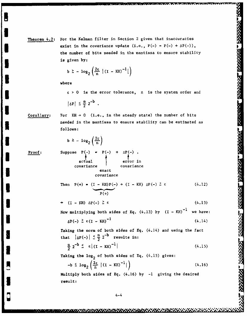
Theorem 4.2: For the Kalman filter in Section 2 given that inaccuracies

exist in the covariance update (i.e., P(-) = P(-) + AP(-)),

the number of bits needed in the mantissa to ensure stability

is given by:

b l 1g2( n 1(I - KH)'I

where

E> 0 is the error tolerance, n is the system order and

< n <-b

Corollary: For KH 0 (i.e., in the steady state) the number of bits

needed in the mantissa to ensure stability can be estimated as

follows:

3 b ~ o 2 C

Proof: Suppose P(-) P(-) + AP(-)

actual I error incovariance covariance

exact

covariance

Then P(+) = (I - KH)P(-) + (I - KH) AP(-) 2- E (4.12)

P(+)

. (I- KH) AP(-) (4.13)

Now multiplying both sides of Eq. (4.13) by (I - KH) - we have:

AP(-) - s(I - KH)-1 (4.14)

Taking the norm of both sides of Eq. (4.14) and using the fact

that IAP(-)l - x 2-b results in:n b < -n2- CI(I - KH) I (4.15)

Taking the log 2 of both sides of Eq. (4.15) gives:

-b < log2 (-. ,(I - KH)-I) (4.16)

Multiply both sides of Eq. (4.16) by -1 giving the desired

result:

4-4

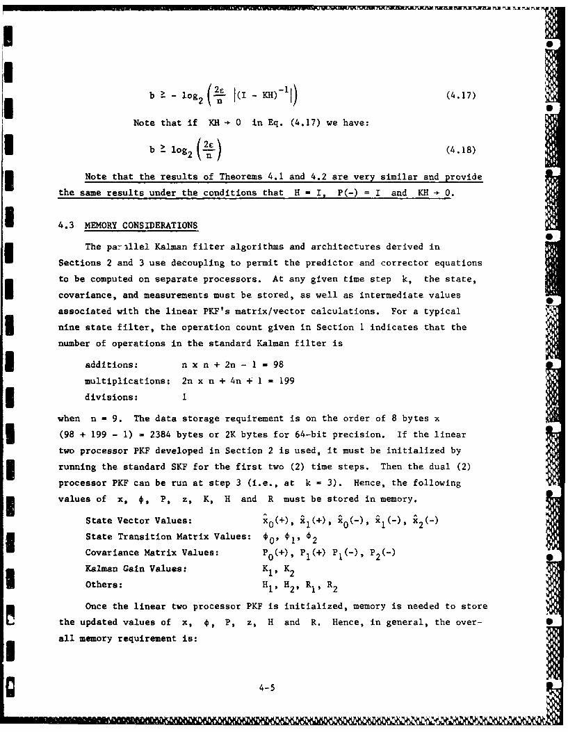
b - log ( I t - KH)1~ (4.17)

I~l og2 n

Note that if KH- 0 in Eq. (4.17) we have:

Ib lo 2 c (4.18)

3 Note that the results of Theorems 4.1 and 4.2 are very similar and provide

the same results under the conditions that H = I, P(-) = I and KH -* 0.

I 4.3 MEMORY CONSIDERATIONS

The pa-illel Kalman filter algorithms and architectures derived in

Sections 2 and 3 use decoupling to permit the predictor and corrector equations

to be computed on separate processors. At any given time step k, the state,

covariance, and measurements must be stored, as well as intermediate valuesassociated with the linear PKF's matrix/vector calculations. For a typical

nine state filter, the operation count given in Section 1 indicates that the

number of operations in the standard Kalman filter is

additions: n x n + 2n - 1 98

multiplications: 2n x n + 4n + 1 f 199

3 divisions: 1

when n - 9. The data storage requirement is on the order of 8 bytes x3 (98 + 199 - 1) - 2384 bytes or 2K bytes for 64-bit precision. If the linear

two processor PKF developed in Section 2 is used, it must be initialized by

3 running the standard SKF for the first two (2) time steps. Then the dual (2)

processor PKF can be run at step 3 (i.e., at k = 3). Hence, the following

3 values of x, 0, P, z, K, H and R must be stored in memory.

State Vector Values: x0 (+), il(+), 0(-), X-), x2(-)

State Transition Matrix Values: c0' I1 2

Covariance Matrix Values: P0(+), P1 (+) PI(-), P2 (-)

Kalman Gain Values: K1 , K2

Others: H1 , H2, R1 , R2

Once the linear two processor PKF is initialized, memory is needed to store

the updated values of x, 4, P, z, H and R. Hence, in general, the over- S

all memory requirement is:

4-5

NL

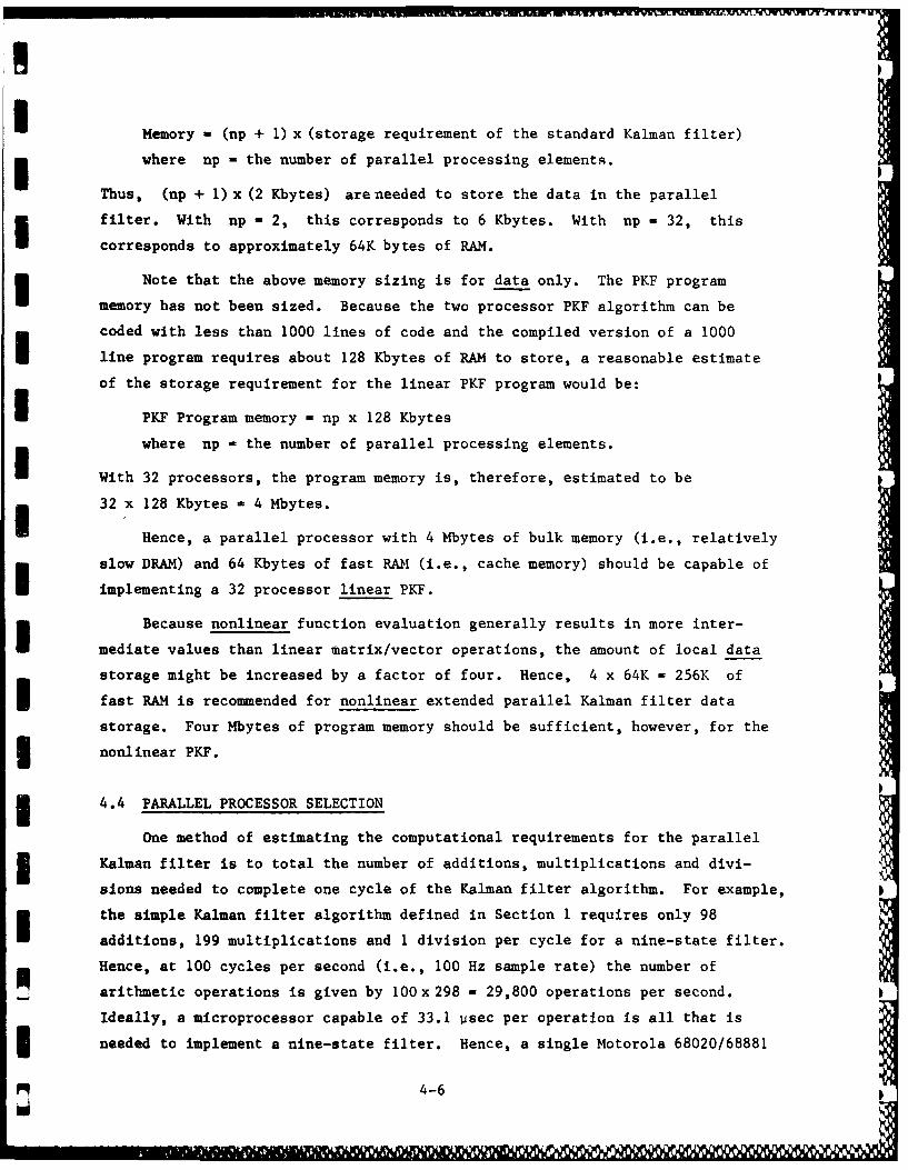
U Memory - (np + 1) x (storage requirement of the standard Kalman filter)

where up - the number of parallel processing elements.

Thus, (np + 1) x (2 Kbytes) are needed to store the data in the parallel

filter. With np - 2, this corresponds to 6 Kbytes. With np - 32, this

corresponds to approximately 64K bytes of RAM.

Note that the above memory sizing is f or data only. The PKF program

memory has not been sized. Because the two processor PKF algorithm can becoded with less than 1000 lines of code and the compiled version of a 1000

I line program requires about 128 Kbytes of RAM to store, a reasonable estimate

of the storage requirement for the linear PKF program would be:

I PKF Program memory - np, x 128 Kbytes

where np - the number of parallel processing elements.

IWith 32 processors, the program memory is, therefore, estimated to be

32 x 128 Kbytes -4 Mbytes.

I Hence, a parallel processor with 4 Mbytes of bulk memory (i.e., relatively

slow DRAM) and 64 Kbytes of fast RAM (i.e., cache memory) should be capable of

implementing a 32 processor linear PKF.

Because nonlinear function evaluation generally results in more inter-

I mediate values than linear maatrix/vector operations, the amount of local datastorage might be increased by a factor of four. Hence, 4 x 64K - 256K of

I fast RAM is recommended for nonlinear extended parallel Kalman filter data

storage. Four Mbytes of program memory should be sufficient, however, for the

3 nonlinear PKF.

4.4 PARALLEL PROCESSOR SELECTION

One method of estimating the computational requirements for the parallel3 Kalman filter is to total the number of additions, multiplications and divi-

sions needed to complete one cycle of the Kalman filter algorithm. For example,

the simple Kalman filter algorithm defined in Section 1 requires only 98

additions, 199 multiplications and 1 division per cycle for a nine-state filter.Hence, at 100 cycles per second (i.e., 100 Hz sample rate) the number of

arithmetic operations is given by 100x 298 - 29,800 operations per second.

Ideally, a microprocessor capable of 33.1 usec per operation is all that is

needed to implement a nine-state filter. Hence, a single Motorola 68020/68881

4-6

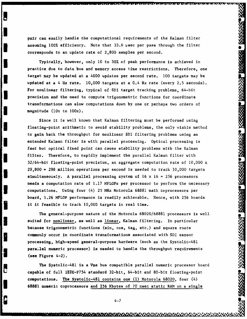
pair can easily handle the computational requirements of the Kalman filter

assuming 100% efficiency. Note that 33.6 usec per pass through the filter

corresponds to an update rate of 2,800 samples per second.

Typically, however, only 10 to 30% of peak performance is achieved in

practice due to data bus and memory access time restrictions. Therefore, one

target may be updated at a 4000 updates per second rate. 100 targets may be

updated at a 4 Hz rate. 10,000 targets at a 0.4 Hz rate (every 2.5 seconds).

For nonlinear filtering, typical of SDI target tracking problems, 64-bit

precision and the need to compute trigonometric functions for coordinate

transformations can slow computations down by one or perhaps two orders of

magnitude (1Ox to 100x).

Since it is well known that Kalman filtering must be performed using

floating-point arithmetic to avoid stability problems, the only viable method

to gain back the throughput for nonlinear SDI filtering problems using an

extended Kalman filter is with parallel processing. Optical processing is

fast but optical fixed point can cause stability problems with the Kalman

filter. Therefore, to rapidly implement the parallel Kalman filter with

32/64-bit floating-point precision, an aggregate computation rate of 10,000 x

29,800 - 298 million operations per second is needed to track 10,000 targets

simultaneously. A parallel processing system of 16 x 16 = 256 processors

needs a computation rate of 1.17 MFLOPs per processor to perform the necessary

computations. Using four (4) 25 MHz Motorola 68881 math coprocessors perboard, 1.26 MFLOP performance is readily achievable. Hence, with 256 boards

3 it it feasible to track 10,000 targets in real time.

The general-purpose nature of the Motorola 68020/68881 processors is well

suited for nonlinear, as well as linear, Kalman filtering. In particular

because trigonometric functions (sin, cos, tag, etc.) and square roots3 commonly occur in coordinate transformations associated with SDI sensor

processing, high-speed general-purpose hardware (such as the Systolic-481

parallel numeric processor) is needed to handle the throughput requirements

(see Figure 4-2).

The Systolic-481 is a Vme bus compatible parallel numeric processor board

capable of full IEEE-P754 standard 32-bit, 64-bit and 80-bit floating-point

computations. The Systolic-481 contains one (1) Motorola 68020, four (4)

I 68881 numeric coprocessors and 256 Kbytes of 70 nsec static RAM on a single

g 4-7 =

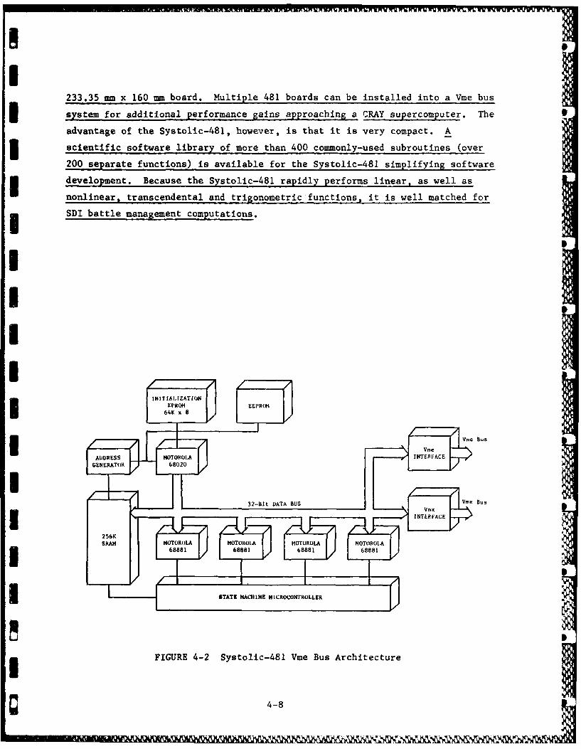
I233.35 mm x 160 mm board. Multiple 481 boards can be installed into a Vme bus

system for additional performance gains approaching a CRAY supercomputer. The

advantage of the Systolic-481, however, is that it is very compact. A3 scientific software library of more than 400 commonly-used subroutines (over

200 separate functions) is available for the Systolic-481 simplifying software

development. Because the Systolic-481 rapidly performs linear, as well as

nonlinear, transcendental and trigonometric functions, it is well matched for

SDI battle management computations.

I

I I EPROM EEPR(*I Bus

IlI

i~~~3-~ DATAR BUS VytlM-8 Vme BuuAcitctr

INE

I STATE MACHINE MICROCONTROLLER

FIGURE 4-2 Systolic-481 Vine Bus Architecture

4-8

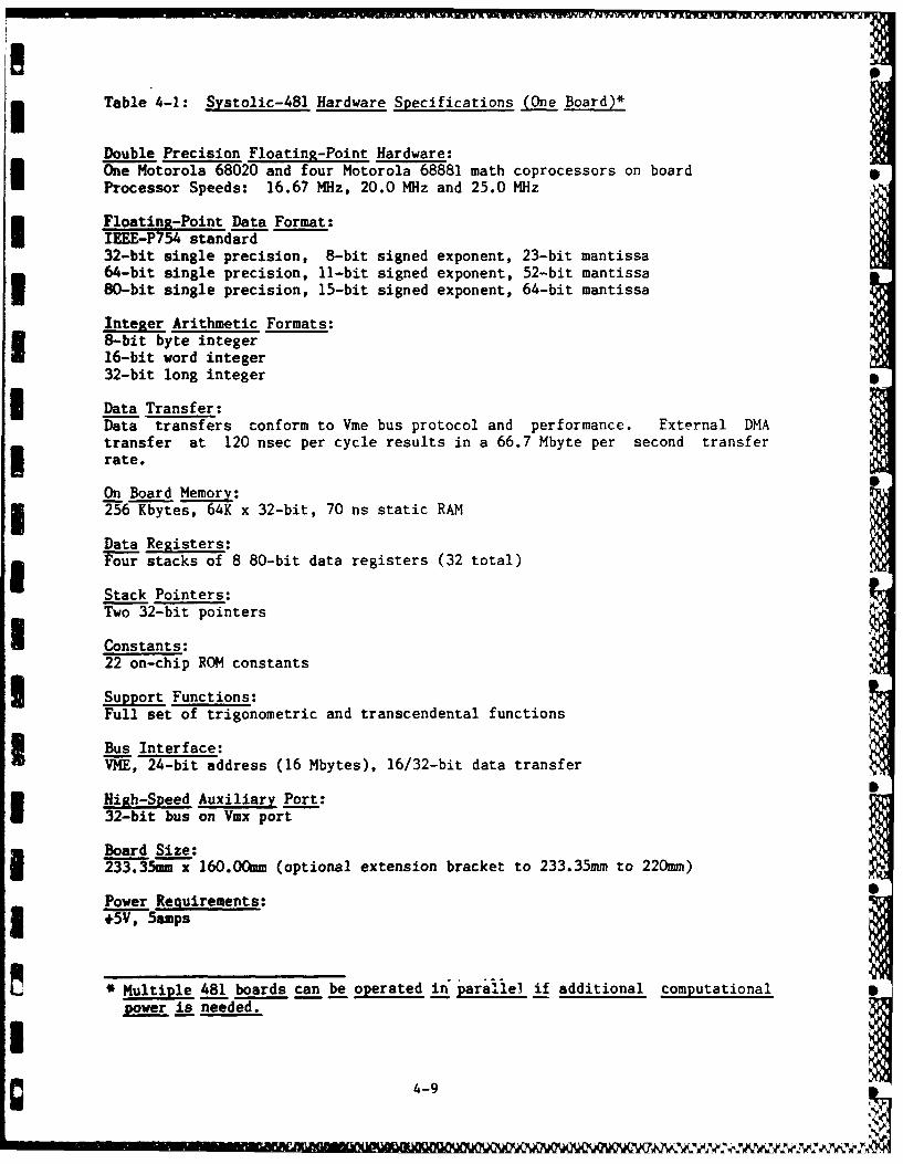
Table 4-1: Systolic-481 Hardware Specifications (One Board)*

Double Precision Floating-Point Hardware:One Motorola 68020 and four Motorola 68881 math coprocessors on boardProcessor Speeds: 16.67 MHz, 20.0 MHz and 25.0 MHz

Floating-Point Data Format:IEEE-P754 standard32-bit single precision, 8-bit signed exponent, 23-bit mantissa64-bit single precision, 11-bit signed exponent, 52-bit mantissa80-bit single precision, 15-bit signed exponent, 64-bit mantissa

Integer Arithmetic Formats:8-bit byte integer16-bit word integer32-bit long integer

Data Transfer:Data transfers conform to Vme bus protocol and performance. External DMAtransfer at 120 nsec per cycle results in a 66.7 Mbyte per second transfer

*r rate.

On Board Memory:256 Kbytes, 64K x 32-bit, 70 ns static RAM

Data Registers:Four stacks of 8 80-bit data registers (32 total)

Stack Pointers:Two 32-bit pointers

U Constants:22 on-chip ROM constants

Support Functions:Full set of trigonometric and transcendental functions

Bus Interface:VME, 24-bit address (16 Mbytes), 16/32-bit data transfer

High-Speed Auxiliary Port:32-bit bus on Vmx port

Board Size:233.35mm x 160.Omm (optional extension bracket to 233.35mm to 220mm)

Power Requirements:+5V, 5amps

' Multiple 481 boards can be operated in parallel if additional computationalpower is needed.

4-9

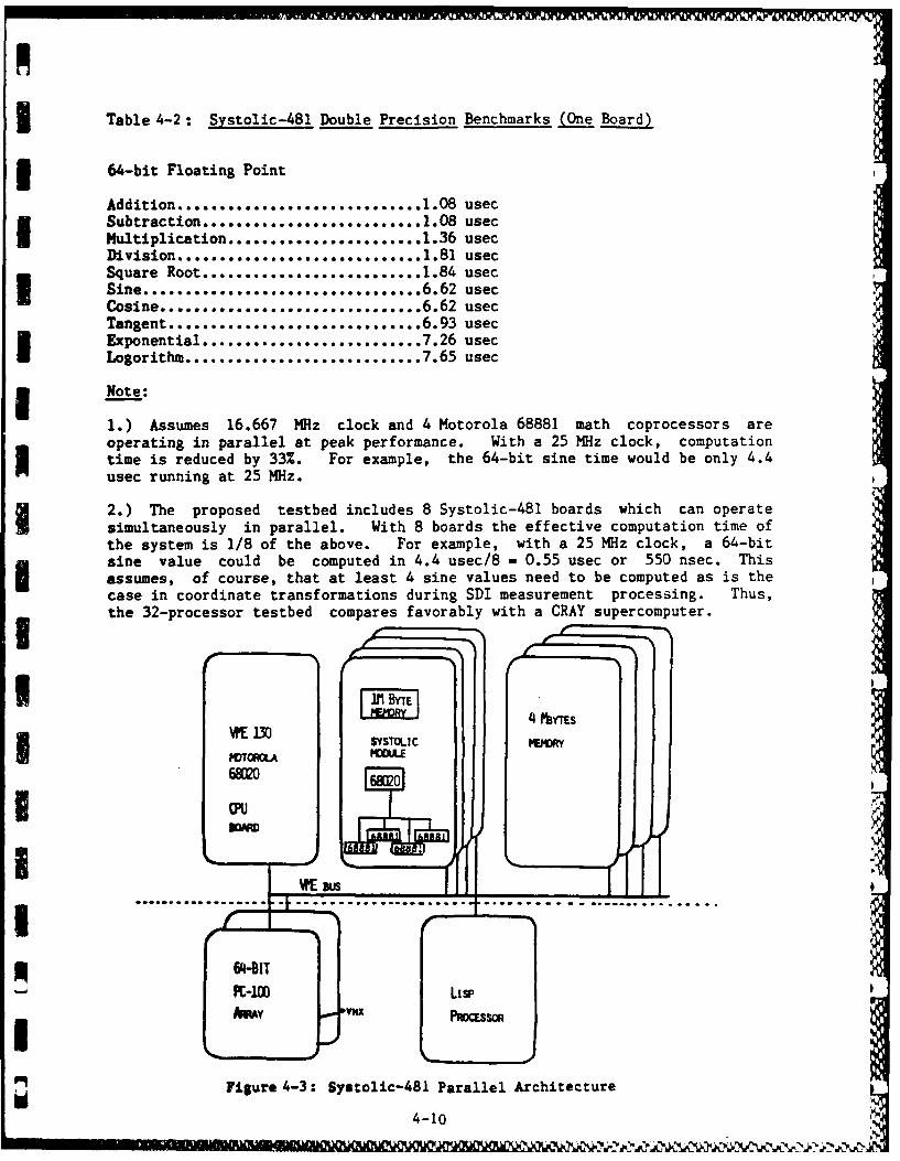
3 Table 4-2: Systolic-481 Double Precision Benchmarks (One Board)

3 64-bit Floating Point

Addition ........................... 1.08 usecI Sutratio .................... 130 usec

Multiplication ...................... 36 usecDivision ...................... 1.81 usec

Square Root......... .......... ......84 usec

Cosine ............................... 6.62 usecTangent............. ... ............ 6.93 usecExponential .......................... 7.26 usecLogorithm ............................ 7.65 usec

* Note:

1.) Assumes 16.667 MHz clock and 4 Motorola 68881 math coprocessors areoperating in parallel at peak performance. With a 25 MHz clock, computationtime is reduced by 33%. For example, the 64-bit sine time would be only 4.4usec running at 25 MHz.

2.) The proposed testbed includes 8 Systolic-481 boards which can operatesimultaneously in parallel. With 8 boards the effective computation time ofthe system is 1/8 of the above. For example, with a 25 MHz clock, a 64-bitsine value could be computed in 4.4 usec/8 - 0.55 usec or 550 nsec. Thisassumes, of course, that at least 4 sine values need to be computed as is thecase in coordinate transformations during SDI measurement processing. Thus,the 32-processor testbed compares favorably with a CRAY supercomputer.

II

R-11By7TMYLA 4 Wa

Figure 4-3: Systolic-481 Parallel Architecture

4-10

SYTOICMEOR

*dSECTION 5

APPLICATION OF THE PKF TO SDI SENSOR TRACK PROCESSING

3 The SDI sensor processing problem can be partitioned into a set of simpler

tasks which when "chained" together provide information to the battle manager.

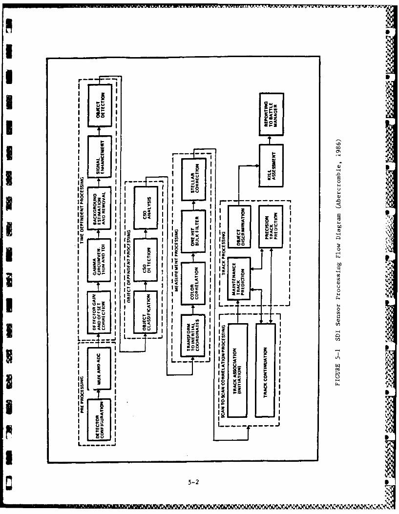
Figure 5-1 illustrates the major parts of the sensor data processing required

by the SDI program. Although each major block in Figure 5-1 can benefit from

high-speed computation, this report is concerned with scan-to-scan correlation

and track processing since Kalman filtering is generally required for precision

tracking. Thus, the remainder of this section formulates the SDI track

processing problem as it applies to the parallel Kalman filtering algorithmsand architectures developed under our Phase I SBIR effort.

5.1 BACKGROUND

To show the effectiveness/payoff of the proposed research it is important

to consider a meaningful SDI problem. The SDI problem should be representative

of typical ballistic missile applications and serve as a baseline to measure

the benefits/accuracy of the Phase I SBIR parallel Kalman filter technology.

3 With this in mind, the following candidate test problem is recommended.

Although this test problem is relatively simple, it illustrates the computations

3 which arise in SDI sensor track processing.

A Simple Test Problem

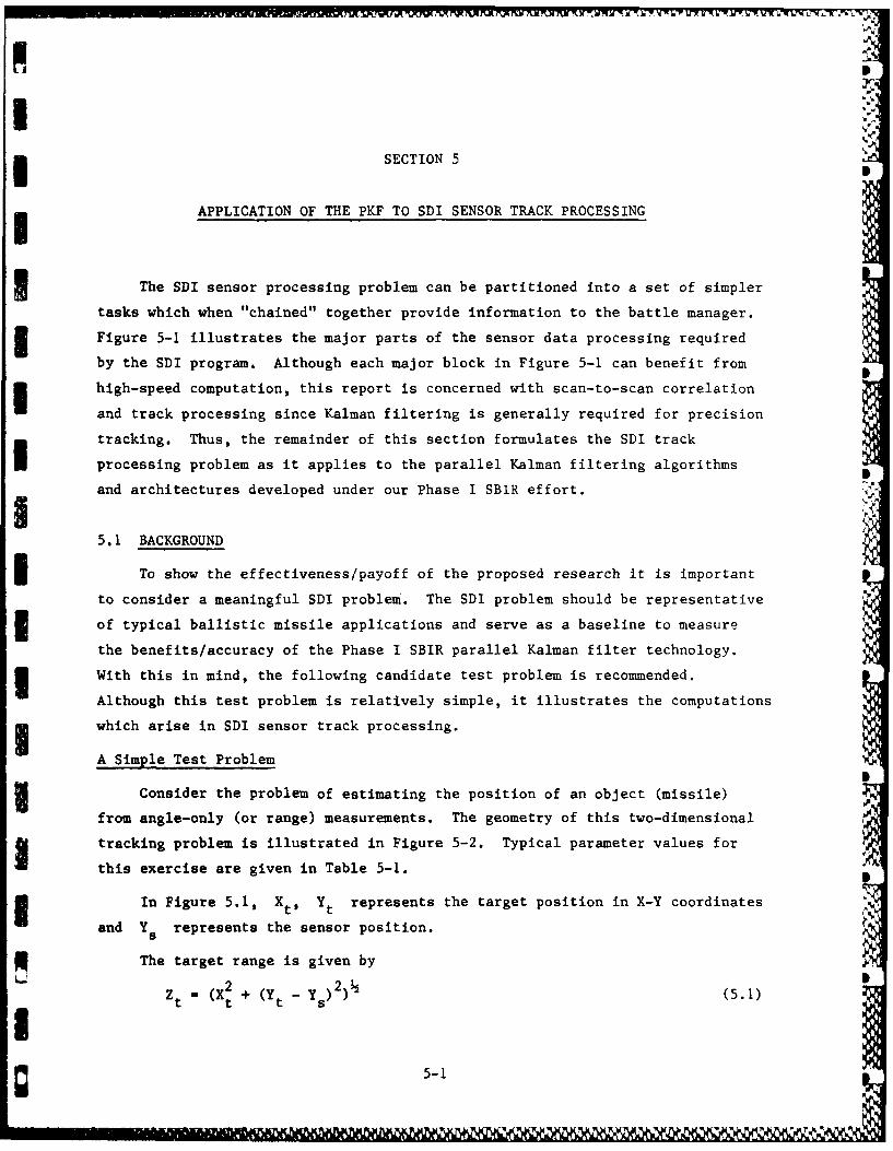
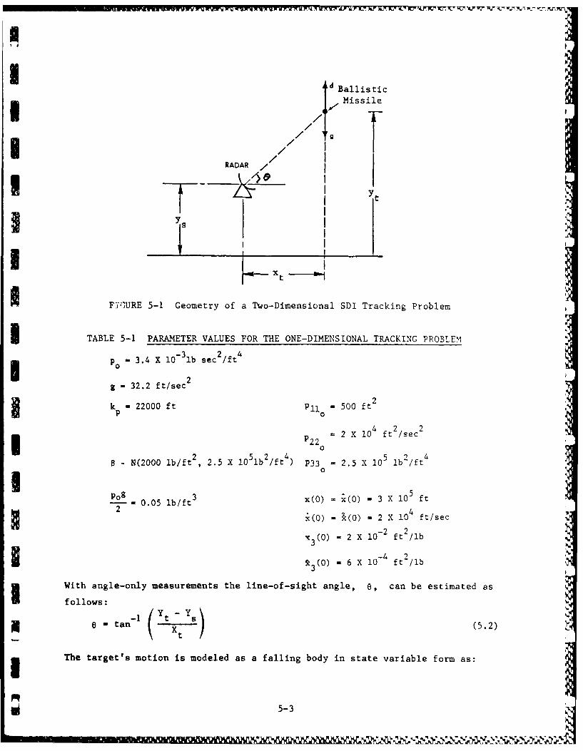
U Consider the problem of estimating the position of an object (missile)from angle-only (or range) measurements. The geometry of this two-dimensional i

tracking problem is illustrated in Figure 5-2. Typical parameter values for

this exercise are given in Table 5-1.

In Figure 5.1, Xt, ft represents the target position in X-Y coordinates

and Y a represents the sensor position.

Tetarget range is given by

- (X2 + (Y - 2 3 (5.1)b

g 5-1

A U t

r -- -K

LI.-

U9-.-- ---

ab A

LuL go - ----

z c- z uIc 'u, I- 1W-C P IcoZ Z 9 1

W!I I ~ I -b

Wau I

I-~

0

w Cc~* : ~~w

5- DI- Z

-EC X.V 1V|n.1 k

d Ballistic

/-Missile

/

/ITRADAR ,.

sI

IF7,1URE 5-1 Geometry of a Two-Dimensional SDI Tracking Problem

I TABLE 5-1 PARAMETER VALUES FOR THE ONE-DIMENSIONAL TRACKING PROBLEM

Po0 lb sec2 /fpO "-3.4 X 103bsc/ft4

9 - 32.2 ft/sec2

k - 22000 ft P11 - 500 ft2

p 2 X 2O4 ft 2/sec

2

IP220

- N(2000 lb/ft , 2.5 X 105 lb 2/ft 4 P33 = 2.5 X 105 lb2/ft4

0

P°g 0.05 Ib/ft 3 x(0) - x(0) - 3 X 10 ft

2(0) . x(O) - 2 X 10& ft/sec

x3(0) - 2 X 10 -2 ft2 /ib

R3(0) - 6 X 10- 4 ft2/lb

With angle-only measurements the line-of-sight angle, 0, can be estimated as

follows:

T e W tan - m Ys (5.2)

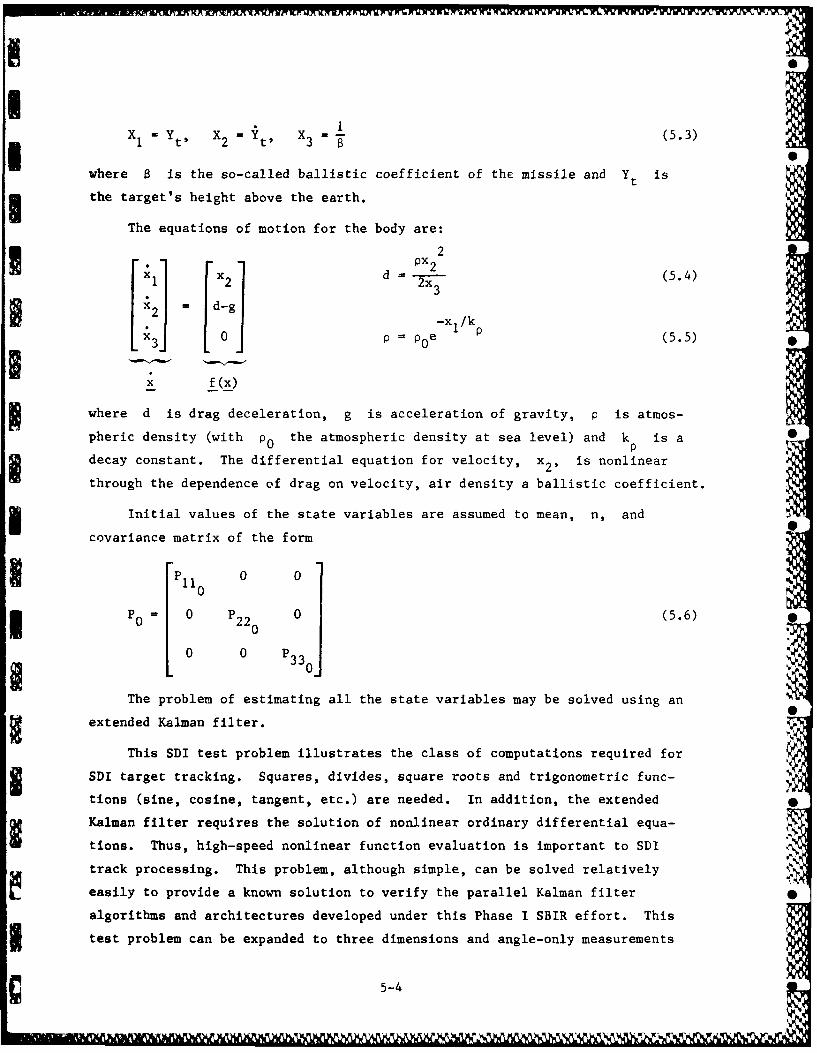
The target's motion is modeled as a falling body in state variable form as:

5-3

2 YW..)

I S

x h Yt t i t , X (5.3)

where 0 is the so-called ballistic coefficient of the missile and Yt isI the target's height above the earth.

The equations of motion for the body are:

x1 x2 d 2x3 (5.4)

x3J 0p e (5.5)

IIf(x)

where d is drag deceleration, g is acceleration of gravity, p is atmos-

pheric density (with p0 the atmospheric density at sea level) and k is aP

decay constant. The differential equation for velocity, x2, is nonlinear

through the dependence of drag on velocity, air density a ballistic coefficient.

Initial values of the state variables are assumed to mean, n, and

covariance matrix of the form

P11 0 0 0

P0 0 P2200 0 (5.6)

0 0 P3 30 "

The problem of estimating all the state variables may be solved using an

extended Kalman filter.

This SDI test problem illustrates the class of computations required for

SDI target tracking. Squares, divides, square roots and trigonometric func-

tions (sine, cosine, tangent, etc.) are needed. In addition, the extended 0

Kalman filter requires the solution of nonlinear ordinary differential equa-

tions. Thus, high-speed nonlinear function evaluation is important to SDI

track processing. This problem, although simple, can be solved relatively

easily to provide a known solution to verify the parallel Kalman filter

algorithms and architectures developed under this Phase I SBIR effort. This

test problem can be expanded to three dimensions and angle-only measurements

C 5-4

of target and sensor position. In this case, the SDI track processing

* problem becomes more nonlinear and involves additional trig functions to be 0

computed during coordinate transformations. The geometry for this case is

* discussed in the next section.

5.2 SDI PROBLEM FORMULATION AND ASPHERICAL EARTH MATH MODEL

U The Kalman filter can be used to update the state estimate of a ballistic

trajectory with angle only measurements. The nonlinear relationship between

the state and the measurements, and the nonlinear dynamics of a ballistic

trajectory, usually require the state estimate to be improved iteratively with

a given measurement set. The problems due to the nonlinearities become more

difficult when the observer is free-falling and more difficult still if the

* observer is located in the plane of the observed trajectory.

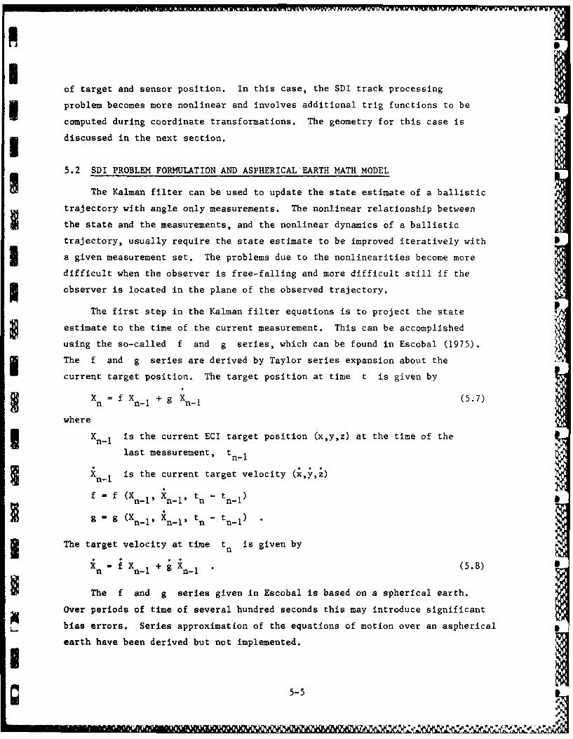
The first step in the Kalman filter equations is to project the state

estimate to the time of the current measurement. This can be accomplished

using the so-called f and g series, which can be found in Escobal (1975).

The f and g series are derived by Taylor series expansion about the

current target position. The target position at time t is given byXn = f Xn- 1 + g Xn- 1 (5.7)

where

SXnI is the current ECI target position (x,y,z) at the time of the

last measurement, tn-I

Xn-I is the current target velocity (xyz)

f f (Xn-l' Xn-l' tn - tn-I)

g " g (Xn-' kXn-1' tn - n- "

The target velocity at time tn is given by

i n - X n- +g Xn-i " (5.8) S

The f and g series given in Escobal is based on a spherical earth.

Over periods of time of several hundred seconds this may introduce significant

bias errors. Series approximation of the equations of motion over an aspherical "

earth have been derived but not implemented.

I

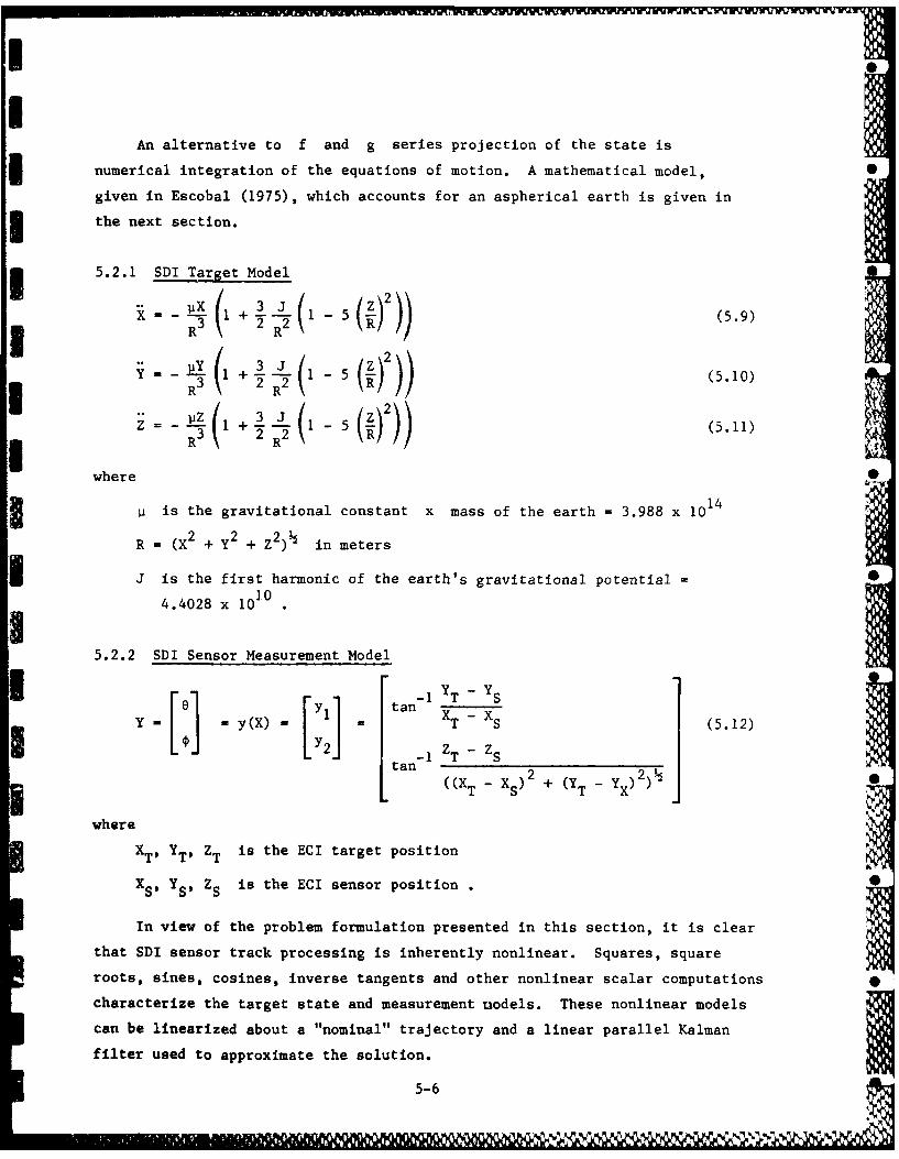
An alternative to f and g series projection of the state is

numerical integration of the equations of motion. A mathematical model, S

given in Escobal (1975), which accounts for an aspherical earth is given in

* the next section.

5.2.1 SDI Target Model

- 1 +- 5 (5.10)

R 3 2R 2 ( R i

S1 -(1 5 ()2)) (5.11)

where

U i is the gravitational constant x mass of the earth = 3.988 x 1014

R (X2 + Y2 + Z2) in meters

J is the first harmonic of the earth's gravitational potential10

4.4028 x 10

5.2.2 SDI Sensor Measurement Model

y(X) - T t a (5.12)SY2 ZT Zs

tan- I1T

M(XT - Xs) 2 + (Y - YX) 2)

where

XT' YT' ZT is the ECI target position

XS, YS, ZS is the ECI sensor position .

In view of the problem formulation presented in this section, it is clear

that SDI sensor track processing is inherently nonlinear. Squares, square

roots, sines, cosines, inverse tangents and other nonlinear scalar computations

characterize the target state and measurement uodels. These nonlinear models

can be linearized about a "nominal" trajectory and a linear parallel Kalman

filter used to approximate the solution.

5-6

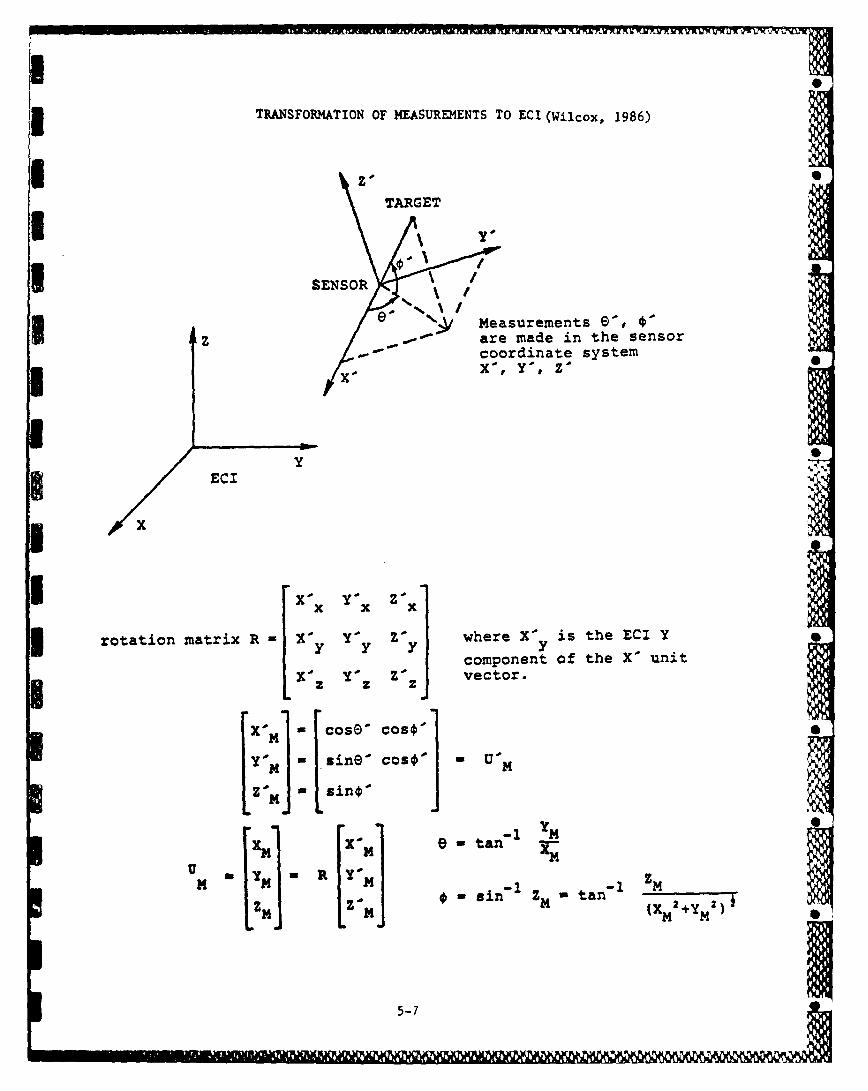
3 TRANSFORMATION OF MEASUREMENTS TO ECI (Wilcox, 1986)

TARGET

U SENSORI

e ~~measurements 9

1z are made in the sensorcoordinate system

EC -I

UX

I0 Xc Yo XZ 0

rotation matrix R X' YC YOyV where X0 is the ECI Y

component of the X' unit

L X0z YAz Z. zi vector.

X0 - cose, COO,"

Y' -sineo cos'* = U~A m

U Z1 -- -1n

(X1

5-7

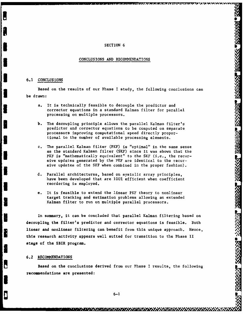
* SECTION 6

3 CONCLUS IONS AND RECOMMENDATIONS

3 6.1 CONCLUSIONS

Based on the results of our Phase I study, the following conclusions can

be drawn:

a. It is technically feasible to decouple the predictor andcorrector equations in a standard Kalman filter for parallelprocessing on multiple processors.

b. The decoupling principle allows the parallel Kalman filter'sU predictor and corrector equations to be computed on separateprocessors improving computational speed directly propor-

* tional to the number of available processing elements.

c. The parallel Kalman filter (PKF) is "optimal" in the same senseas the standard Kalman filter (SKF) since it was shown that theI PKF is "mathematically equivalent" to the SKF (i.e., the recur-sive updates generated by the PKF are identical to the recur-sive updates of the SKF when combined in the proper fashion).

Id. Parallel architectures, based on systolic array principles,have been developed that are 100% efficient when coefficient3 reordering is employed.

e. It is feasible to extend the linear PKF theory to nonlineartarget tracking and estimation problems allowing an extendedU Kalman filter to run on multiple parallel processors.

3 In summary, it can be concluded that parallel Kalman filtering based on

decoupling the filter's predictor and corrector equations is feasible. Both

linear and nonlinear filtering can benefit from this unique approach. Hence,

this research activity appears well suited for transition to the Phase IIstage of the SEIR program.

6.2 RECOMMENDATIONS

Based on the conclusions derived from our Phase I results, the following

recommendat ions are presented:

0 6-1

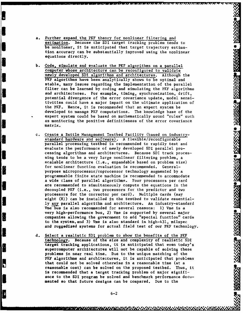
a. Further expand the PKF theory for nonlinear filtering andestimation. Because the SDI target tracking problem tends tobe nonlinear, it is anticipated that target trajectory estima-tion accuracy can be substantially improved using the nonlinearequations directly.

b. Code, simulate and evaluate the PKF algorithms on a parallelcomputer whose architecture can be reconfigured to validatenewly developed SDI algorithms and architectures. Although thePKF algorithms have been analytically shown to be optimal andstable, many issues regarding the implementation of the parallelfilter can be learned by coding and simulating the PKF algorithmsand architectures. For example, timing, synchronization, drift,potential divergence of the error covariance update, model sensi-tivities could have a major impact on the ultimate application ofthe PKF. Hence, it is recommended that an expert system bedeveloped to manage PKF computations. The knowledge base of theexpert system could be based on mathematically sound "rules" suchas monitoring the positive definitieness of the error covariancematrix.

c. Create a Battle Management Testbed Facility (based on industry-standard hardware and software). A flexible/reconfigurableparallel processing testbed is recommended to rapidly test andevaluate the performance of newly developed SDI parallel pro-cessing algorithms and architectures. Because SDI track proces-sing tends to be a very large nonlinear filtering problem, a 0scalable architecture (i.e., expandable based on problem size)for nonlinear function evaluation is recommended. General-purpose microprocessor/coprocessor technology augmented by aprogrammable finite state machine is recommended to accommodatea wide class of parallel algorithms. Four processors per cardare recommended to simultaneously compute the equations in thedecoupled PKF (i.e., two processors for the predictor and twoprocessors for the corrector per card). Multiple cards (sayeight (8)) can be installed in the testbed to validate essential-ly any parallel algorithm and architecture. An industry-standardVme bus is also recommended for several reasons: 1) Vme is avery high-performance bus, 2) Vme is supported by several major Bcompanies allowing the government to add "special function" cardsto the system, and 3) Vme is also standard in high-431, milspecand ruggedized systems for actual field test of our PKF technology.

d. Select a realistic SDI problem to show the benefits of the PKFtechnology. Because of the size and complexity of realistic SDItarget tracking applications, it is anticipated that even today's

supercomputer architectures will not be capable of solving theseproblems in near real time. Due to the unique matching of thePKF algorithms and architectures, it is anticipated that problemsthat could not be solved otherwise in a reasonable time (at areasonable cost) can be solved on the proposed testbed. Thus, itis recommended that a target tracking problem of major signifi-ance to the SDI program be solved and benchmark performance docu-mented so that future designs can be compared. Due to the

6-2

IU ' I I1 111 1 I'l I, 1 11 !!

' i'"special" architecture of the Battle Management testbed it isanticipated that it can be the standard to improve upon for thenext five (5) yearb.

6.3 SUMMARY

Based on the results in this report it is clear that the PKF theory is

well developed, mature and ready to proceed to full-scale validation on a

parallel processing testbed. Because the PKF technology has been needed to

solve several applications in the DoD for more than a decade, it is antici-

pated that once fully developed this technology can benefit several sectors

of the DoD. This is possible because the necessary technology has only

recently been available to transition the PKF theory into practice. Hence,

Systolic Systems would be pleased to continue this program under Phase II

I of the SBIR program.

I

I L.C./ ; 2 "" '"' - A '

IIII

I

g6-3

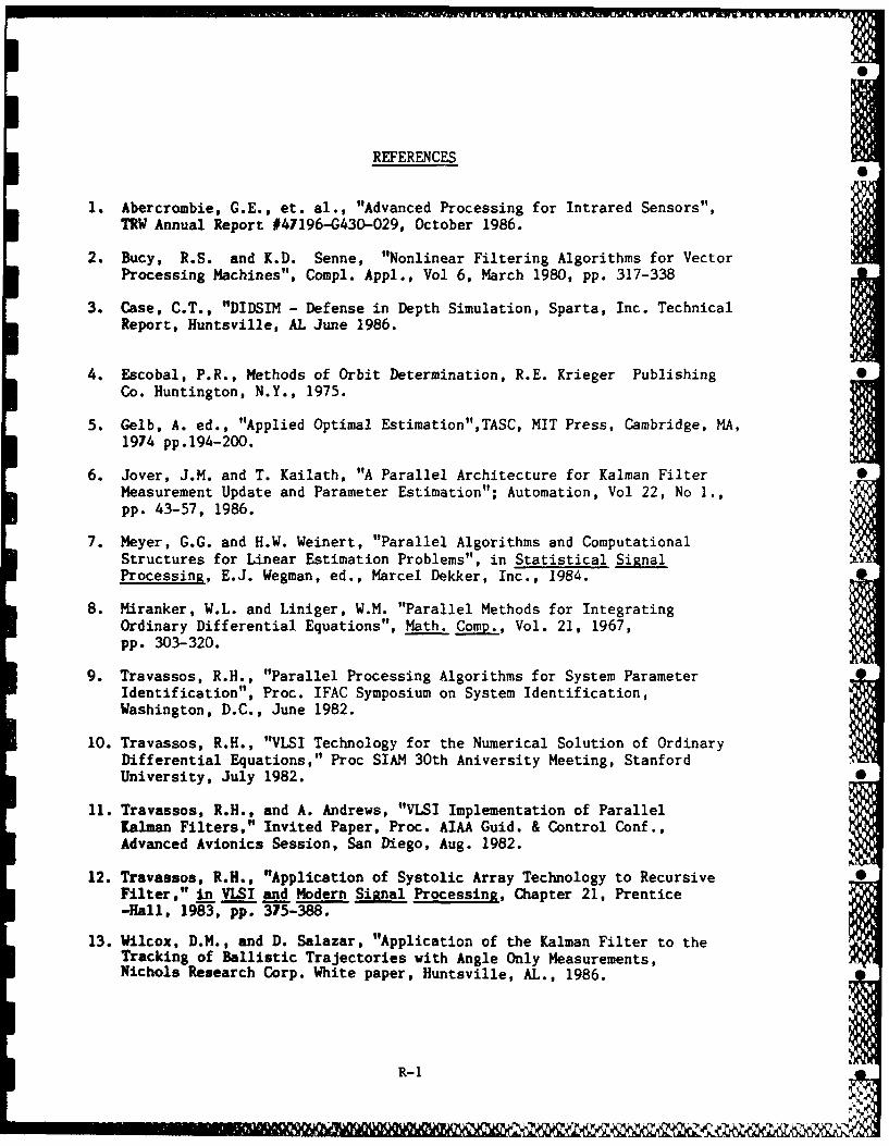
REFERENCES

1. Abercrombie, G.E., et. al., "Advanced Processing for Intrared Sensors",TRW Annual Report #47196-G430-029, October 1986.

2. Bucy, R.S. and K.D. Senne, "Nonlinear Filtering Algorithms for VectorProcessing Machines", Compl. Appl., Vol 6, March 1980, pp. 317-338

3. Case, C.T., "DIDSIM - Defense in Depth Simulation, Sparta, Inc. TechnicalReport, Huntsville, AL June 1986.

4. Escobal, P.R., Hethods of Orbit Determination, R.E. Krieger PublishingCo. Huntington, N.Y., 1975.

5. Gelb, A. ed., "Applied Optimal Estimation",TASC, MIT Press, Cambridge, MA,1974 pp.194-200.

6. Jover, J.M. and T. Kailath, "A Parallel Architecture for Kalman Filter 0Measurement Update and Parameter Estimation"; Automation, Vol 22, No 1.,pp. 43-57, 1986.

7. Meyer, G.G. and H.W. Weinert, "Parallel Algorithms and ComputationalStructures for Linear Estimation Problems", in Statistical SignalProcessing, E.J. Wegman, ed., Marcel Dekker, Inc., 1984.

8. Miranker, W.L. and Liniger, W.M. "Parallel Methods for IntegratingOrdinary Differential Equations", Math. Comp., Vol. 21, 1967,pp. 303-320.

9. Travassos, R.H., "Parallel Processing Algorithms for System ParameterIdentification", Proc. IFAC Symposium on System Identification,Washington, D.C., June 1982.

10. Travassos, R.H., "VLSI Technology for the Numerical Solution of OrdinaryDifferential Equations," Proc SIAM 30th Aniversity Meeting, StanfordUniversity, July 1982. 0

11. Travassos, R.H., and A. Andrews, "VLSI Implementation of ParallelKalman Filters," Invited Paper, Proc. AIAA Guid. & Control Conf.,Advanced Avionics Session, San Diego, Aug. 1982.

12. Travassos, R.H., "Application of Systolic Array Technology to Recursive •Filter," in VLSI and Modern Signal Processing, Chapter 21, Prentice-Hall, 1983, pp. 375-388.

13. Wilcox, D.M., and D. Salazar, "Application of the Kalman Filter to theTracking of Ballistic Trajectories with Angle Only Measurements,Nichols Research Corp. White paper, Huntsville, AL., 1986.

R-1

1111111 m il

KR1~

//IA?

* -- - - - - - - - - - - - 0 - 0 0 -

V