Errors, Errors, Uncertainties in Uncertainties in Data AssimilationData Assimilation

François-Xavier LE DIMETFrançois-Xavier LE DIMET

Université Joseph Université Joseph Fourier+INRIAFourier+INRIA

Projet IDOPT, Grenoble, Projet IDOPT, Grenoble, FranceFrance

AcknowlegmentAcknowlegment

Pierre Ngnepieba ( FSU)Pierre Ngnepieba ( FSU) Youssuf Hussaini ( FSU)Youssuf Hussaini ( FSU) Arthur Vidard ( ECMWF)Arthur Vidard ( ECMWF) Victor Shutyaev ( Russ. Acad. Sci.)Victor Shutyaev ( Russ. Acad. Sci.) Junqing Yang ( LMC , IDOPT)Junqing Yang ( LMC , IDOPT)

Prediction: What Prediction: What information is information is

necessary ?necessary ? ModelModel

- law of conservation mass, energylaw of conservation mass, energy- Laws of behaviourLaws of behaviour- Parametrization of physical processesParametrization of physical processes

Observations in situ and/or remoteObservations in situ and/or remote Statistics Statistics ImagesImages

Forecast..Forecast..

Produced by the integration of the Produced by the integration of the model from an initial condition model from an initial condition

Problem : how to link together Problem : how to link together heterogeneous sources of informationheterogeneous sources of information

Heterogeneity in :Heterogeneity in : Nature Nature Quality Quality DensityDensity

Basic ProblemBasic Problem

U and V control U and V control variables, V being variables, V being and error on the and error on the modelmodel

J cost functionJ cost function U* and V* minimizes U* and V* minimizes

JJ

Optimality SystemOptimality System

P is the adjoint P is the adjoint variable.variable.

Gradients are Gradients are couputed by couputed by solving the adjoint solving the adjoint model then an model then an optimization optimization method is method is performed.performed.

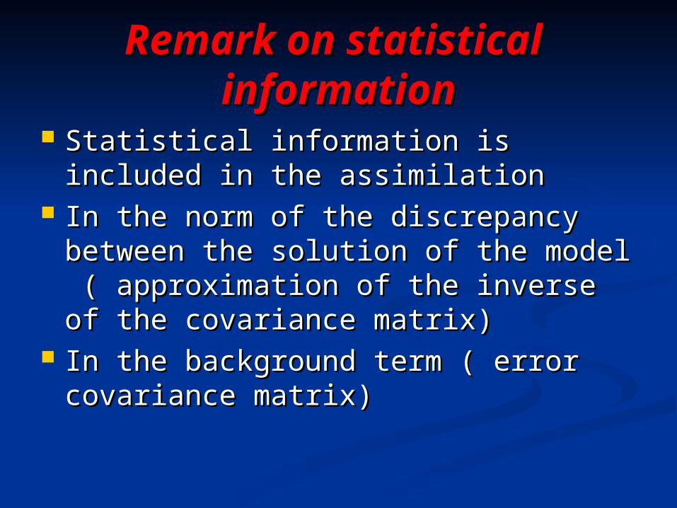
Remark on statistical Remark on statistical informationinformation

Statistical information is included in Statistical information is included in the assimilationthe assimilation

In the norm of the discrepancy In the norm of the discrepancy between the solution of the model between the solution of the model ( approximation of the inverse of the ( approximation of the inverse of the covariance matrix)covariance matrix)

In the background term ( error In the background term ( error covariance matrix)covariance matrix)

Remarks:Remarks:

This method is used since May 2000 for This method is used since May 2000 for operational prediction at ECMWF and operational prediction at ECMWF and MétéoFrance, Japanese Meteorological MétéoFrance, Japanese Meteorological Agency ( 2005) with huge models ( 10 Agency ( 2005) with huge models ( 10 millions of variable.millions of variable.

The Optimality System countains all the The Optimality System countains all the available information available information

The O.S. should be considered as a The O.S. should be considered as a « Generalized Model »« Generalized Model »

Only the O.S. makes sense.Only the O.S. makes sense.

ErrorsErrors On the modelOn the model

Physical approximation (e.g. parametrization of Physical approximation (e.g. parametrization of subgrid processes)subgrid processes)

Numerical discretizationNumerical discretization Numerical algorithms ( stopping criterions for Numerical algorithms ( stopping criterions for

iterative methodsiterative methods On the observationsOn the observations

Physical measurementPhysical measurement SamplingSampling Some « pseudo-observations », from remote Some « pseudo-observations », from remote

sensing, are obtained by solving an inverse sensing, are obtained by solving an inverse problem.problem.

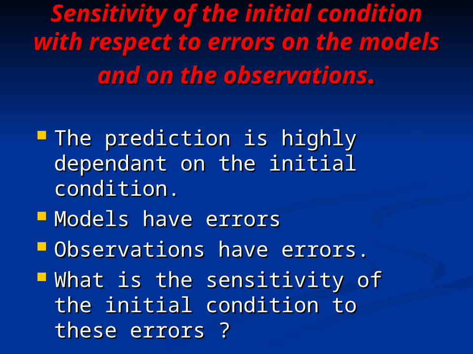
Sensitivity of the initial Sensitivity of the initial condition with respect to condition with respect to

errors on the models and on errors on the models and on

the observationsthe observations..

The prediction is highly dependant The prediction is highly dependant on the initial condition.on the initial condition.

Models have errorsModels have errors Observations have errors.Observations have errors. What is the sensitivity of the initial What is the sensitivity of the initial

condition to these errors ? condition to these errors ?

Optimality System : including errors on Optimality System : including errors on the model and on the observationthe model and on the observation

Second order adjointSecond order adjoint

Models and DataModels and Data

Is it necessary to improve a model if Is it necessary to improve a model if data are not changed ?data are not changed ?

For a given model what is the For a given model what is the « best » set of data?« best » set of data?

What is the adequation between What is the adequation between models and data?models and data?

A simple numerical A simple numerical experimentexperiment..

Burger’s equation with Burger’s equation with homegeneous B.C.’shomegeneous B.C.’s

Exact solution is knownExact solution is known Observations are Observations are

without errorwithout error Numerical solution with Numerical solution with

different discretizationdifferent discretization The assimilation is The assimilation is

performed between T=0 performed between T=0 and T=1and T=1

Then the flow is Then the flow is predicted at t=2.predicted at t=2.

Partial ConclusionPartial Conclusion

The error in the model is introduced The error in the model is introduced through the discretizationthrough the discretization

The observations remain the same The observations remain the same whatever be the discretizationwhatever be the discretization

It shows that the forecast can be It shows that the forecast can be downgraded if the model is upgraded.downgraded if the model is upgraded.

Only the quality of the O.S. makes Only the quality of the O.S. makes sense.sense.

Remark 1Remark 1 How to improve How to improve

the link between the link between data and models?data and models?

C is the operator C is the operator mapping the space mapping the space of the state of the state variable into the variable into the space of space of observationsobservations

We considered the We considered the liear case.liear case.

Remark 2 : ensemble predictionRemark 2 : ensemble prediction

To estimate the impact of uncertainies on To estimate the impact of uncertainies on the prediction several prediction are the prediction several prediction are performed with perturbed initial performed with perturbed initial conditionsconditions

But the initial condition is an artefact : But the initial condition is an artefact : there is no natural error on it . The error there is no natural error on it . The error comes from the data throughthe data comes from the data throughthe data assimilation processassimilation process

If the error on the data are gaussian : If the error on the data are gaussian : what about the initial condition?what about the initial condition?

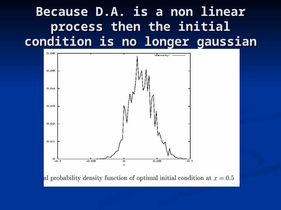
Because D.A. is a non linear Because D.A. is a non linear process then the initial condition process then the initial condition

is no longer gaussianis no longer gaussian

Control of the errorControl of the error

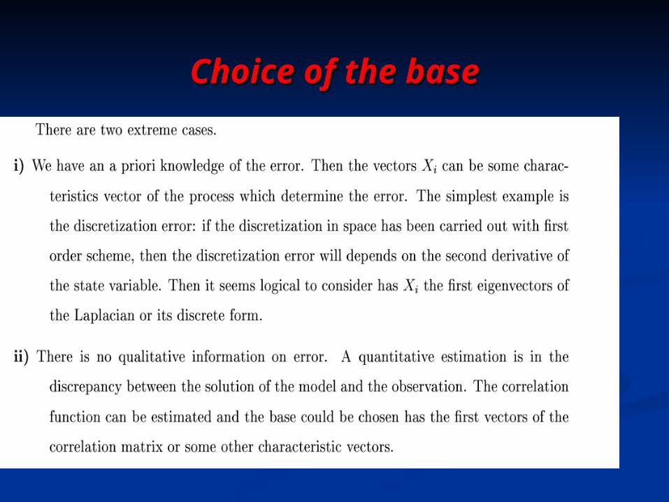
Choice of the baseChoice of the base

Remark Remark .. The model has several sources of errorsThe model has several sources of errors Discretization errors may depends on the second Discretization errors may depends on the second

derivative : we can identify this error in a base of derivative : we can identify this error in a base of the first eigenvalues of the Laplacianthe first eigenvalues of the Laplacian

The systematic error may depends be estimated The systematic error may depends be estimated using the eigenvalues of the correlation matrixusing the eigenvalues of the correlation matrix

Numerical experimentNumerical experiment

With Burger’s equationWith Burger’s equation Laplacian and covariance matrix Laplacian and covariance matrix

have considered separately then have considered separately then jointlyjointly

The number of vectors considered in The number of vectors considered in the correctin term variesthe correctin term varies

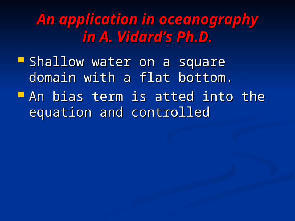
An application in An application in oceanographyoceanography

in A. Vidard’s Ph.D.in A. Vidard’s Ph.D. Shallow water on a square domain Shallow water on a square domain

with a flat bottom.with a flat bottom. An bias term is atted into the An bias term is atted into the

equation and controlledequation and controlled

Sequential model :

Cost Function

Evolution of the bias :

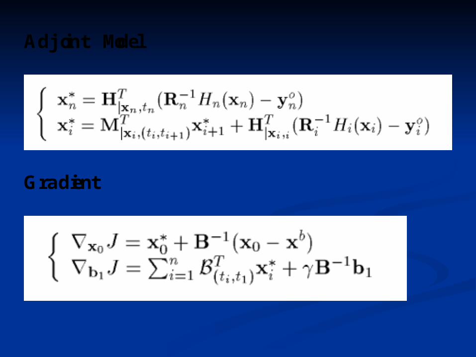
Adjoint Model

Gradient

Model

Relative vorticity

Potential

Model is forced by sinusoidal winds

Preconditioning using the covariance matrix , thecontrol variable becomes :

Cost function

RMS ot the sea surface height with or RMS ot the sea surface height with or without control of the biaswithout control of the bias

An application in hydrologyAn application in hydrology(Yang Junqing )(Yang Junqing )

Retrieve the evolution of a riverRetrieve the evolution of a river With transport+sedimentationWith transport+sedimentation

Physical phenomena

•fluid and solid transport

•different time scales

1. Shallow-water equations

2. Equation of constituent concentration

3. Equation of the riverbed evolution

⎪⎪⎩

⎪⎪⎨

⎧

=⋅∇+∂∂

−Δ+∇−=×+∇⋅+∂∂

.0)(

,)( 1

hvt

h

vh

vCvkzgvkfvv

t

vD

r

rr

rrrrrr

)()()()hS( *' SSShkhSv

t−+∇⋅∇=⋅∇+

∂∂ αωr

.)( *1 b

b gSSt

Z r⋅∇−−=

∂∂ αωρ

NN

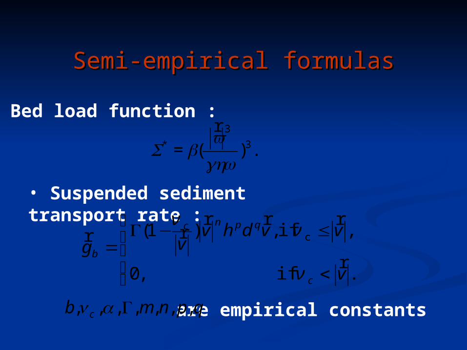
Semi-empirical formulasSemi-empirical formulas

• Bed load function :

• Suspended sediment transport rate :

.)( 3

3

*

ωghv

bSr

=

⎪⎩

⎪⎨

⎧

<

≤−Γ=

. if ,0

, if,)1( c

v

vvdhvvg

c

qpnc

br

rrrrr

ν

νν

are empirical constantsqpnmb c ,,,,,,, Γαν

An example of simulationAn example of simulation

• Domain : km 100 km 100 ו Space step : 2 km in two directions• Time step : 120 seconds

Initial river bed

Simulated evolution of river bed (50 years)

⎪⎩

⎪⎨⎧

Ω==

×Ω⋅+=

. on ,)0(

],,0[ on ),,()),,((

UtX

TtxVBtxUXFdt

dX

Model error estimation controlled system

• model

• cost function dtVVXtxVUXCVUJ

T

obs ),),,,((2

1),(

0

2 >Ν<+−⋅= ∫ Ωβ

• optimality conditions .0)( ,0)( ** == VJGradUJGrad VU

• adjoint system(to calculate the gradient)

⎪⎩

⎪⎨

⎧

=

−⋅=⎥⎦⎤

⎢⎣⎡∂∂

+

.0)(

),(*

TP

XXCCXX

F

dt

dPobs

tt

⎩⎨⎧

Ν+−=

−=

. )(

),0()(

VPBVJGrad

PUJGradt β

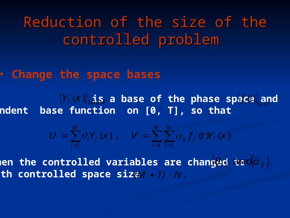
Reduction of the size of the Reduction of the size of the controlled problem controlled problem

• Change the space bases

Suppose is a base of the phase space and is time-dependent base function on [0, T], so that

{ } Mii xY ≤≤1)( { }Njj tf

≤≤1)(

)()( ),(1 11

xYtfVxYU ij

M

i

N

jiji

M

ii ∑∑∑

= ==

== αθ

then the controlled variables are changed to with controlled space size

{ } { } and iji αθ

.N1)(M ×+

Optimality conditions for the Optimality conditions for the estimation estimation

of model errors after size reductionof model errors after size reduction

⎪⎩

⎪⎨

⎧

>Ν<=

=

⇔

=⎪⎭

⎪⎬

⎫

⎪⎩

⎪⎨

⎧

>Ν+−<=

><−=

∫

∑∫

−−T

ijt

ij

lk ijklklt

T

ij

ii

dtYfPB

P

dtYfYfPBJGrad

YPJGrad

0

11

,0

,

,0)0(

0,), ()(

,),0()(

βα

αβα

θ

If P is the solution of adjoint system, we search for optimal values of to minimize J :{ } { } , iji αθ

Problem : how to choose the spatial base ?

• Consider the fastest error propagation direction

• Amplification factor

• Choose as leading eigenvectors of

• Calculus of

- Lanczos Algorithm

{ })(xYi

⎪⎩

⎪⎨⎧

==

=

.)0(

,)(^

^

HtX

HMTX T

22

2^

2 ,)(

H

HHMM

H

TXA TT

t ><==

{ })(xYi

.TTt

T MMS ={ })(xYi

Numerical experiments with another Numerical experiments with another basebase

• Choice of “correct” model :

- fine discretization: domain with 41 times 41 grid

points

• To get the simulated observation - simulation results of ‘correct’ model

• Choice of “incorrect” model :

- coarse discretization: domain with 21 times 21 grid

points

The difference of potential field between two models after 8

hours’ integration

Experiments without size reduction (1083*48) :

the discrepancy of models at the end of integration

before optimization

after optimization

Experiments with size reduction (380*48) :

the discrepancy of models at the end of integration

before optimization

after optimization

Experiments with size reduction (380*8) :

the discrepancy of models at the end of integration

before optimization

after optimization

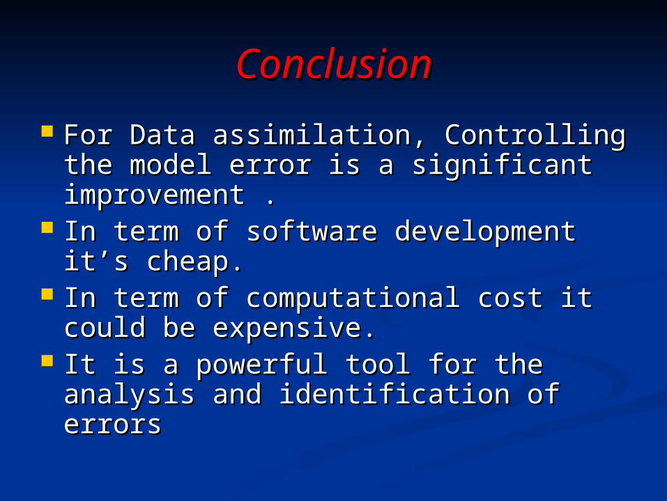
ConclusionConclusion

For Data assimilation, Controlling For Data assimilation, Controlling the model error is a significant the model error is a significant improvement .improvement .

In term of software development it’s In term of software development it’s cheap.cheap.

In term of computational cost it In term of computational cost it could be expensive.could be expensive.

It is a powerful tool for the analysis It is a powerful tool for the analysis and identification of errorsand identification of errors